WORKING PAPERS IN ECONOMICS

No. 06/05

LIV OSLAND, INGE THORSEN AND JENSPETTER GITLESEN

HOUSING PRICE GRADIENTS IN AGEOGRAPHY WITH ONEDOMINATING CENTER

Department of Economics ________________________ U N I V E R S I T Y OF B E R G E N

Housing price gradients in a geography with one dominating

center∗

Liv Osland†, Inge Thorsen‡, and Jens Petter Gitlesen§

March 17, 2005

∗This paper has benefited from comments by Viggo Nordvik and Espen Bratberg.†Stord/Haugesund University College, Bjørnsonsgt. 45, 5528 Haugesund, Norway (e-mail: liv.osland@hsh.no,

fax: +47 52702765, phone: +4752702768)‡Stord/Haugesund University College, Bjørnsonsgt. 45, 5528 Haugesund, Norway§University of Stavanger, N-4036 Stavanger, Norway.

1

Abstract

We primarily focus on explaining housing prices and predicting housing price gradientsin a Norwegian region with one dominating center (Stavanger). For such a geography spatialseparation can be represented in a hedonic regression equation by a function of traveling dis-tance from the city center. Several functions are tested, and some alternatives provide botha satisfying goodness-to-fit, consistent coefficient estimates, and intuitively reasonable pre-dictions of housing price gradients. Still, not all commonly used functions are recommended.Spatial autocorrelation is removed when the hedonic function is properly specified.

Keywords: hedonic regression model, housing attributes, functional representation of spatialseparation, spatial autocorrelation, housing price gradient, capitalization

2

1 Introduction

Housing price gradients represent important input to studies covering a wide range of regionaland urban policy issues. One example is that investments in transportation infrastructure mightcause reductions in traveling times to the cbd (central business district) and capitalize throughproperty values. Our results are relevant in for instance studies related to constructing newroads (tunnels/bridges), changing speed limits or in analyzing investments inducing increasedcapacity and reduced queues on existing links.

Many empirical studies have aimed at finding rent gradients, land value gradients and/orhousing price gradients. Ball (1973) and Bartik and Smith (1987) review several studies ofthe determinants of housing prices. In a few studies the variable indicating access to workcame out with an insignificant sign, and occasionally a contra-intuitive sign was reported. Suchresults are explained either by multicollinearity problems, or by the fact that the study areain some cases involve a restricted urban area rather than a housing market area. Anotherreason for such results is that modern metropolitan areas tend to be multicentric. Dubin (1991)takes as his starting point the saying that ”the three most important determinants of housingprices are location, location and location”, and states that including distance from the cbd in ahedonic price function is the most common way of examining the effect of accessibility. Heikkilaet al. (1989) state that most studies on land values have shown a significant and stronglynegative land value gradient, when the hedonic price function is properly specified. Richardson(1988) also states that the main reason for insignificant or counter-intuitive results stems froma misspecified hedonic price function. This result is demonstrated in Waddell et al. (1993), whofind that distance to the cbd is significant even when access to multiple employment centersand other nodes are accounted for. Adair et al. (2000) on the other hand claim that transportaccessibility has limited explanatory power in modern segregated and segmented cities, andthey recommend that studies focusing on the effect of spatial separation on housing prices areperformed in homogenous markets.

In line with this tradition our main ambition is to study the functional form of the rele-vant gradient in a coherent labor and housing market area with one dominating center (Sta-vanger). Our study area is appropriate for this purpose, since it comes close to the geographyunderlying the traditional trade-off theory, while most empirical studies have considered morecomplex metropolitan areas. The breakthrough of this strand of analysis is represented by the“access-space-trade-off” model (Alonso 1964). Basically this model starts with a homogeneouslandscape. There exists one central business district (cbd) where all employment and businessactivities are located. The households make two kinds of decisions: How much land do theywant in what distance from the city centre? Households thus decide how much they are willingto pay for land by changing commuting time. This theoretical tradition of urban land use hasbeen extended in many directions, see for instance Mills (1967), Muth (1969), Fujita (1986), andBrueckner (1987). The basic idea remains, however, represented by a steadily declining price ofland and houses with increasing distance from the cbd.

Our empirical approach is based on the so-called hedonic method. The method is built on theidea that heterogeneous goods constitute of a number of attributes. Examples of attributes re-lated to housing are the quality and size of the house. Achieved utility depends on the provisionsof different attributes. When different combinations and amounts of attributes yield utility, andwhen there exist supply and demand for individual attributes, the hedonic approach introducesthe implicit price structure of such attributes. These prices are defined as the increase in thetotal price of the corresponding good resulting from a marginal increase in the amount of therelevant attribute. The theoretical foundation of the hedonic method was established in Rosen(1974). Rosen showed that the hedonic price function is an equilibrium-function, enveloped by

3

consumers’ so-called ”bid-functions” and suppliers’ ”offer-functions”. Rosen’s theory also offersthe conditions for being able to interpret the implicit prices as the marginal willingness to payfor the respective attributes. For a review on hedonic analysis of housing markets, see Sheppard(1999).

A long tradition and a lot of literature in empirical hedonic housing market studies is devotedto the problem of defining a suitable delimitation of a housing market, both spatially and withrespect to relevant types of dwellings, see for instance Straszheim (1974), Rothenberg et al.(1991), and Whitehead (1999). This problem is not addressed in this paper. The housingmarket in our prosperous study area is fairly homogenous. Spatially, the region is considered asone coherent housing and labor market area. Data on spatial labor market interaction clearlyindicate that this is a reasonable assumption. We focus on one type of house only, that isprivately owned single-family houses. In many cities the supply of this housing type is scarcerelative to the situation in surrounding areas. This is not the case for Stavanger, where theproportion of privately owned single family houses is not markedly different from the average inNorway. On the other hand, the supply of other housing types, like terraced houses, is markedlyunderrepresented in more peripheral, rural areas of the region. Hence, such categories are lessappropriate for the purpose of studying spatial variation in housing prices in a wide area.

In this paper we primarily search for general results on the relationship between housingprices and traveling time from the cbd. We are more concerned with predictability than inachieving a highest possible explanatory power, and we adopt a macroscopical perspective ofthe geography. Our macroscopical perspective is represented by a specific zonal subdivisionof the geography, and the fact that we consider interzonal rather than intrazonal variations inhousing prices. The zonal subdivision of the geography corresponds to the most detailed spatiallevel for which official Norwegian data are available. Data restrictions represent the main reasonwhy we consider a relatively macroscopical description of the geography. Still, we stronglydoubt that the additional insight and explanatory power resulting from a more disaggregatedrepresentation of the geography would be reasonably related to the enormous effort and resourcesrequired on data collection, if at all practically possible. For some spatially related attributes,like for instance the view, or the distance to nursery school, a relatively high degree of interzonalhomogeneity can be expected. Many attributes are reasonably equally present in most of the(postal delivery) zones that we consider. We will of course account for the effect of some basicresidence-specific attributes (internal living area, lot size, age of building etc.), but we ignorethe impact of intrazonal location-specific amenities and services.

Section 2 provides documentation of our data, and the region is described and explained tobe very appropriate for our purpose. As a benchmark for evaluating the impact of traveling timeon housing prices, we start out by considering some non-spatial modeling alternatives. Thosealternatives are described in Section 3, while the corresponding results are presented in Section4. We also evaluate model performance for alternative delimitations of the geography. In Section5 we evaluate traveling time and physical distance as alternative measures of spatial separation,once again for alternative delimitations of the geography. Section 6 focuses on different functionalrepresentation of the relationship between housing prices and traveling time. The evaluation isbased both on explanatory power, and from the ability to predict reliable housing price gradientsfor a given set of values on other attributes than spatial separation from the cbd. Finally, inSection 7 we offer some concluding remarks.

4

2 The region and the data

2.1 The region

The study area in this paper is the southern parts of Rogaland, which is the southernmost countyin Western Norway. This represents an integrated region with a connected road transportationnetwork. There are 13 municipalities in the region, and each municipality is divided into postaldelivery zones. All in all the region is divided into 98 (postal delivery) zones, as indicated inFigure 1. A strongly dominating part of journeys-to-work is made by cars. As an indicatorof (commuting) distances by car, there is 79 km from the centre of Stavanger to Egersund inthe south. According to our data the corresponding estimated shortest route traveling time is69 minutes. This delimits a fairly large region in a hedonic context, motivated from the factthat our basic ambition is to study the relationship between labour and housing markets. Theregion comes close to what is defined as “an economic area” in Barkley et al. (1995), witha relatively self-contained labor market, and a relatively large central place (Stavanger) whichinfluences on economic activity in a peripheral region. The high degree of intra-dependencywithin the region is very much due to physical, topographical, transportation barriers, thatlengthen travel distances, and thereby deter economic relationships with other regions. Theregion is delimited by the North Sea in the west, fjords in the north and the east, while thesouthern delimitation is an administrative county border in a sparsely populated, mountainousarea. Appendix A provides a list of municipalities and postal delivery zones, with correspondingfigures of population and employment in 2001.

Stavanger

Rennesøy

Sola

Randaberg

Sandnes

Klepp

Hå

Time

Gjesdal

Bjerkreim

Eigersund Lund

Sokndal

1

2

3

4

415

46

45

47

48

49

50

61

63

5360

51

52

62

5455

72

71

73

70

6956

84

82

83

74

787675

77

81

80

79

88

87

86

89

85

91

90

99

98

95

96

97

94

92

93

43

386

4039

78

910

20

15

17

131112

14

21 18

16

19

24

26

22

27

23

25

2830

29

3436

31

3537

44

33

32

5859

57

67

6665

64 68

42

Figure 1: The division of the region into municipalities and zones

This prosperous region has experienced considerable population and employment growth overthe last three decades. This is to a large extent due to the growth of petroleum based activities.

5

As mentioned in the introduction Stavanger is the dominating city centre of the region. Since1970 population has increased by about 36% in Stavanger, while the corresponding populationgrowth has been 91% in municipalities adjacent to Stavanger, and 49% in municipalities moreperipherally located in the region. The corresponding population growth in Norway was about17%. Considering such figures, it is important to know that land is relatively scarce in Stavanger,which is the fourth largest city in Norway. The suburbanization of both housing construction,shopping centers, and manufacturing firms has benefited the neighboring municipalities. Theregion has largely developed from employment growth in and close to the Stavanger city center.This contributes to make it appropriate for reaching reliable parameter estimates reflecting the”access-space-trade-off” rather than local characteristics of the central place system.

The geography we consider is not literally corresponding to the geography underlying thetraditional trade-off theory, with a monocentric city in a featureless plain landscape. Still,it is probably hard to find geographies that come considerably closer to such a theoreticalconstruction. The region has developed towards a central place system with centers at differentlevels, but Stavanger indisputably has a very dominating position, with a far higher rank thanother centers in this system. This is not quite reflected in population figures for the municipalitiesin the region, since large parts of adjacent municipalities belong to the Stavanger residentialarea. This also applies for Sandnes, which is the second largest central place in this region, a lotlarger than the third largest central place. The rapid population growth in Sandnes is explainedprimarily from the fact that it is located only 16 kilometers from Stavanger.

Land has become scarce in areas adjacent to the city center of Stavanger, and here hasbeen a tendency that basic sector jobs have been decentralized to locations more distant fromthe cbd area. A large part of such activities is related to the administration of petroleumactivities. The city center of Stavanger still has a dominating position concerning the supply ofspecific urban facilities, represented for instance by leisure and cultural services, and by shoppingopportunities. The area has not developed into the characteristic multi-nodal structure observedin many metropolitan areas.

The fact that considerable commuting flows are observed from most parts of the region toStavanger indicates that it makes good sense to consider the region as a suitable housing andlabor market. Neither the labor market nor the housing market in any part of the region aresignificantly influenced by urban areas in other regions. The population growth throughout theregion reflects the trade-off between housing prices and commuting costs. As mentioned abovethe municipalities adjacent to Stavanger has experienced a rapid population growth over thelast decades. As a result of innovations in the transportation network, there is a tendency thatthis growth is spread to areas located in a longer physical distance from the Stavanger cityarea. As an example, Time is currently one of the municipalities in Norway that experiencesthe largest absolute increase in the number of dwellings. This is far from being matched bya corresponding increase in local employment opportunities. The traveling time from Bryne,the municipality center, to Stavanger is about 32 minutes, and Bryne is considered by manyhouseholds to represent an attractive combination of traveling time and housing prices.

2.2 Data on housing prices

The housing market data consist of transactions of privately owned single-family houses in theperiod from 1997 through the first half of 2001. According to Statistics Norway, on average 52%of all sales in Norway are single-house dwellings. Our sample of 2788 observations representsapproximately 50% of the total number of transactions of privately owned single-family housesin the region during the relevant period. In estimating the model we ignore transactions whereinformation is missing for some variable(s). A lack of information on lot-size is the main reasonwhy our sample is not even larger. To some degree the lack of information is positively related

6

to the age of the houses. For other variables there is no indication in our data that our sampleis not reasonably representative for the total number of transactions. We have in particularsearched for possible spatial variation in the missing information. Despite some signs of varyinginter-municipality practice in reporting data from transactions to official registers, we find nosubstantial tendency of systematic variation in available information across space.

The data on housing prices and housing attributes come from two different sources:

• Information on housing sales prices, postal codes, site in square meters, and type of buildingis collected from the national land register in Norway. This register is called the GAB-register. GAB is an abbreviation of ground parcel, address and building, and containsinformation on all ground parcels and buildings in Norway.

• Information on internal living space, garage, age of building, number of toilets and bath-rooms as well as the time of sale is collected from Statistics Norway. These data come froma questionnaire that is sent to everyone who has bought a freeholder dwelling in Norway.

Each building is located on a postal code, and we use the postal codes to add informationon distances and number of residents/employees.

Some information could be collected from both the GAB-register and Statistics Norway. Inorder to check which source is the most reliable, information was gathered from a third source,a local estate agent. Simple linear regressions were run between variables that existed in allthree data-sets. If R2 and the beta coefficient in the linear regression are 1, there is a perfect fitbetween the data-sets. This kind of analysis enabled us to discover serious problems with theliving area variable found in the GAB-register, and the postal codes from Statistics Norway. Bycollecting data from three different sources, it was thus possible to verify that the postal codesin GAB were reliable, and that the variable for living area had to be collected from StatisticsNorway.

In Appendix B we present descriptive housing market statistics. As expected both theaverage sales-price and the standard deviation are higher in Stavanger than in the other parts ofthe region. The dwellings with the smallest lot-size tend to be among the oldest in the sample,and the majority of those dwellings are located in Stavanger.

2.3 Data on population and employment

The division of the region into zones corresponds to the most detailed level of informationwhich is available on individual residential and work location. The information is based on theEmployer-Employee register, and provided for us by Statistics Norway. Access to data on zonalpopulation is gained through the Central Population Register in Statistics Norway.

2.4 The matrix of physical distances and traveling times between the zones

The matrices of physical distances and traveling times were prepared for us by the NorwegianMapping Authority. The calculations were based on the specification of the road network intoseparate links, with known distances and speed limits. Distances are given from a data basewith an accuracy of ±2 meters for each link. In calculating traveling times it is accounted forthe fact that actual speed depends on road category. Information of speed limits and road cate-gories is converted into traveling times through instructions (adjustment factors for specific roadcategories) worked out by the Institute of Transport Economics. The centre of each (postal de-livery) zone is found through detailed information on residential densities and the road network.Finally, both the matrix of distances and the matrix of traveling times is constructed from ashortest route algorithm. Interzonal distances are measured between zonal centers.

7

3 Non-spatial hedonic model formulations

In this study we do not attempt to account for accessibility to recreational facilities and shoppingopportunities, and we ignore environmental conditions, location-specific amenities, and aestheticattributes. This practice is partly explained from the fact that we consider interzonal ratherthan intrazonal variations in housing prices. Our approach is implicitly based on the assumptionthat such housing and location specific (micro-locational) attributes are not varying systemati-cally across the zones. In other words we implicitly assume that the regional variation in suchattributes can also be found within a zone, and that there is insignificant spatial variation inzonal average values.

We distinguish between two categories of attributes. One category is the physical attributesof the specific dwelling, the other is related to the location-specific attributes. In a general formthe corresponding hedonic price equation can be expressed as follows:

Pit = f(zsit, zlit) (1)

Here

Pit = the price of house i in year t

zsit = value of dwelling-specific structural attribute s for house i in year t; s = 1, ...S, i = 1, ...n

zlit = value of location-specific attribute l for house i in year t; l = 1, ...L, i = 1, ...n

All the hedonic regression results to be presented in this paper involve the same set ofdwelling-specific attributes, zsi, which are defined in Table 1.

Table 1: List of non-spatial variablesVariable Operational definitionREALPRICE selling price deflated by the consumer price index, base year is 1998AGE age of buildingLIVAREA living area measured in square metersLOTSIZE lot-size measured in square metersGARAGE dummy variable indicating presence of garageNUMBTOIL number of toilets in the buildingREBUILD dummy variable indicating whether the building has been rebuilt/renovated

The ambition to capture the trade-off between housing market prices and labor marketinteraction calls for a large study area. As a working hypothesis we claim that unbiased estimatesof this relationship cannot be based on a truncated specification of the market area. We preparefor a discussion on this by estimating the alternative model formulations for the following threesubdivisions of the geography:

• The entire region

• The four most centrally located municipalities in the northern parts of the region (Sta-vanger, Sandnes, Randaberg and Sola, see the map in Figure 1)

• Stavanger

8

This corresponds to a natural subdivision of the geography, where Stavanger represents thecbd, while the four most centrally located municipalities represent an extended urban area ina relatively monocentric spatial structure. We have also experimented with the mathematicalrepresentation of the relationship between dependent and independent variables. As in mostother empirical studies of the housing market we find that log-linear model formulations aresuperior to linear and semi-logarithmic model specifications. Only results based on log-linearspecifications are presented.

4 Results based on non-spatial model formulations

Least squares estimation results based on the non-spatial model formulations are presentedin Table 2. Model M1 refers to a specification where the estimation is based on data fromthe entire region, while the estimation of M2 is based on data from the four most centrallylocated municipalities, and M3 is based on data from Stavanger. To obtain a high number ofobservations, the data are aggregated through time. In order to account for increases in housingprices during the period, changing intercepts are introduced through dummy variables for eachyear. The dummy for 1998 is excluded in order to avoid perfect multicollinarity between thesevariables.

In general the coefficient estimates in Table 2 are supposedly biased, since important in-formation on location is omitted from the model formulation underlying the results. This isespecially evident for the variable LOTSIZE. The estimate of the coefficient corresponding tothis variable has a counter-intuitive sign in the model specification based on data covering theentire region. We will return to a discussion of this result in Section 5.

Let βA denote the coefficient attached to the variable AGE, while βAR is attached to AGE ·REBUILD. A significantly positive estimate of βAR means that the negative impact of AGEupon housing price is reduced. It is intuitively reasonable, however, that |βA| > |βAR|, meaningthat AGE has a negative influence on housing price, even if the house has been rebuilt.

White’s general test (see for instance Greene 2003) is performed to test for heteroskedasticity.Since χ2

0,05 = 16, 919 it follows from Table 2 that the hypothesis of homoskedasticity is rejectedin all model specifications. In order to make reliable inferences on the least square estimateswhen heteroskedasticity is present, the reported standard errors in all models will be estimatedby the robust estimator of variance. In our data, however, this robust estimator of variancedoes not produce results that deviate much from estimates based on the ordinary least squaresestimator.

According to Odland(1988) a test for spatial autocorrelation in the residuals should alwaysbe applied when using spatial data. Spatial heterogeneity implies violations of the assumptionof a spherical error covariance matrix (Anselin 1988). This means that spatial heterogeneityrepresents an efficiency problem. If positive spatial dependence in the errors is present theestimated values of R2, t- and F -values will be artificially high (Odland 1988). Inferences mayhence be misleading and tests for heteroskedasticity may have reduced validity (Anselin and Rey1991). According to Anselin (1988) and Odland (1988) the reason for spatial heterogeneity liesin the estimated model. This could be due to a poor functional representation of the relevantproblem, and/or to the possibility that our list of independent variables fails to account forrelevant spatial peculiarities or interdependencies in the data.

Moran’s I is reported as a descriptive measure of whether there exists spatial autocorrelationin the residuals1. In the computation a binary row standardized weight matrix is used to define

1Moran’s I values are computed in the program R by using R-packages developed by Roger Bivand, NorwegianSchool of Economics and Business Administration.

9

Table 2: Results based on non-spatial modeling specificationsM1 M2 M3

Constant 11.83 11,77 11,26(0,179) (0,183) (0,136)

LOTSIZE -0,0154 0,0644 0,0952(0,0136) (0,0129) (0,0159)

AGE -0,045 -0,0397 -0,0461(0,0075) (0,0076) (0,0080)

AGE·REBUILD 0,0171 0,0130 0,0154(0,0040) (0,0036) (0,0043)

GARAGE 0,081 0,052 0,0435(0,0149) (0,0134) (0,0168)

LIVAREA 0,4330 0,3774 0,4665(0,0418) (0,0459) (0,0341)

NUMBTOIL 0,2235 0,1701 0,1226(0,0267) (0,0268) (0,0243)

YEARDUM97 -0,1181 -0,1250 -0,1523(0,0178) (0,0177) (0,2410)

YEARDUM99 0,1565 0,1454 0,1305(0,0188) (0,0176) (0,0232)

YEARDUM00 0,2835 0,2787 0,2582(0,0178) (0,0173) (0,0218)

YEARDUM01 0,3120 0,3127 0,2834(0,0185) (0,0185) (0,0234)

n 2788 2051 1188R2 0,5221 0,5944 0,6606R2-adj. 0,5204 0,5924 0,6578L -580 7 57APE 312233 277302 273133White test statistic 278 135 110Moran’s I 0,3590 0,1554 0,0718Standard Normal Deviate (zI) 184 71 26

Note: Results based on observations from the period 1997-2001, robust standard errors in parentheses. M1

refers to a specification where the estimation is based on data from the entire region, while the estimation of M2

is based on data from the four most centrally located municipalities, and M3 is based on data from Stavanger.

10

the relation between observations. Zones which have common borders in the geography areneighbors. All houses within a zone are also neighbors. A house is not a neighbor to itself.

The values of Moran’s I range approximately from -1 to 1. Positive values indicate positiveautocorrelation. A value of zero (or more precisely, − 1

n−1 (Florax et al. 2002)), may indicate nospatial autocorrelation. In Table 2 we have also reported values of the standard normal deviate(zI) that is constructed from values of the mean and the variance of the Moran statistic (seefor example Anselin (1988) for details on the estimation of such values). Corresponding to thistransformed variate the null hypothesis is the absence of spatial autocorrelation in the residuals.The alternative hypothesis is spatial autocorrelation of some unspecified kind (Anselin 1988).This means that the null is rejected at the 5% significance level if zI > 1, 645. It follows fromTable 2 that the null is rejected in all the non-spatial model specifications. It also follows fromthe table that (positive) spatial autocorrelation is strongest when estimation is based on datafrom the entire region. According to the values of Moran’s I a natural hypothesis is that thesystematic pattern of spatial interdependencies across zones is positively related to how largepart of the region that is considered.

In addition to R2 we have reported values of two measures to evaluate the goodness of fitabilities of various model alternatives. L is the log-likelihood value. The Average PredictionError (APE) is explicitly based on a comparison between the observed and the predicted housing

prices; APE =∑

i(|P̂i−Pi|)n . Here P̂i is the predicted price of house i, while n is the observed

number of houses. APE has an obvious interpretation, but this measure is not appropriate forstatistical testing and to discriminate between alternative model specifications.

According to Table 2 the non-spatial independent variables explain more of the variation inhousing prices the smaller part of the region that is considered. This justifies the hypothesisthat information on spatial characteristics like distances is particularly important in studiesbased on a wide delimitation of the study area. If the study area is restricted for instanceto a specific urban area distances probably contribute less to the explanation of housing pricevariation, and non-spatial housing attributes explain more of the variation in housing prices. Thecorresponding hypothesis is that short distances within a sub-area have only marginal impact onindividual spatial labour market behavior and housing prices. We will return to this discussionin forthcoming sections, where spatial characteristics are explicitly taken into account.

Notice from Table 2 that log-likelihood values apparently are obscure in the logarithmicmodel specifications. Positive log-likelihood values might in general result in rare cases fordensity functions with very small variance, allowing for density values exceeding 1,0. Such casestypically are met in problems where dependent variables are defined for a relatively small rangeof high values. In our study the logarithm of housing prices defines a function that is very flatfor the relevant range of values, with correspondingly low variance.

5 Results based on hedonic model formulations including trav-eling time from the labor market center in the region

In order to estimate the housing-price gradient, it is necessary to identify the center of thegeography. Since we focus on the trade-off between housing prices and commuting costs it isreasonable to find the labor market center. According to Plaut and Plaut (1998) much of theempirical literature in the field assumes that the location of the center is known in advance. Inour study the location of the labor market center is found endogenously. For this purpose weintroduced a gravity based accessibility measure. Assume that distance (traveling time fromorigin j to destination k, djk) appears through a negative exponential function in the definitionof the accessibility measure, and let σ be the weight attached to distance; σ < 0. The Hansen

11

type of accessibility measure (Hansen 1959), Sij is then defined as follows:

Sj =w∑

k=1

Dk exp(σdjk) (2)

Here, Dk represents the number of jobs (employment opportunities) in destination (zone) k.The measure Sij is based on the principle that the accessibility of a destination is a decreasingfunction of relative distance to other potential destinations, where each destination is weightedby its size, or in other words the number of opportunities available at the specific location.Hence, it can be interpreted as an opportunity density function.

It is not a priori obvious that the zones in the city center of Stavanger represent the labormarket center of the region. In addition there is in particular a high labour demand originat-ing from an area hosting for instance large industrial firms and administrative units related topetroleum activities. This industrial area is located in between the Sandnes and Stavanger.Another category of zones with high labor market accessibility are those located in an inter-mediate position between the center of Stavanger and the mentioned industrial area. Still, ourresults reveal a clear tendency that model performance is best when centrally located zones inStavanger is chosen as the labor market center. To be more specific zone 10 is found to representa natural labor market center in the region.

As another starting point for the results to be presented in this section we found that modelperformance is significantly better when traveling time rather than physical distance is used asthe measure of spatial separation.

Studies of journeys-to-work report significant distance deterrence effects, see for instanceThorsen and Gitlesen (1998). One general problem in empirical spatial interaction studies is tochoose an appropriate specification of the distance deterrence function. Some studies are basedon a power function (dβp

ij ), while others are based on an exponential deterrence function (eβedij ).In both specifications the distance deterrence parameter is of course negative; βp < 0 and βe < 0.The choice of the distance deterrence function has been considered to be essentially a pragmaticone in the literature, see for instance Nijkamp and Reggiani (1992). For some problems thismight be correct, but some studies have concluded that the appropriateness of the functionalform should be critically examined, see for instance a study of US migration flows in Fik andMulligan (1998).

Combined with the three alternative delimitations of the geography (the entire region, thefour most centrally located municipalities, and Stavanger), we consider two alternative specifi-cations of the spatial separation function:

M8-M10: a negative exponential function, three alternative delimitations of the geography

M11-M13: a power function specification, three alternative delimitations of the geography

The models which are linear in all parameters are estimated by ordinary least squares,whereas the models which are nonlinear in at least one parameter is estimated by using nonlinearleast squares and maximum likelihood estimation. The general rule is that the result fromthe general least squares estimations are used as starting values for the maximum likelihoodestimation. In all the nonlinear models the two methods give identical results.

In the previous section we found that especially the coefficient related to lot size variedconsiderably with respect to the subdivision of the geography. In the case where estimation isbased on data from the entire region we even found that this coefficient has a counter-intuitive,negative, sign. This is probably a result of the fact that non-spatial model specifications ignorethe positive covariation between lot size and the distance from the cbd. Such counter-intuitiveresults do not appear when relevant measures of spatial separation are included.

12

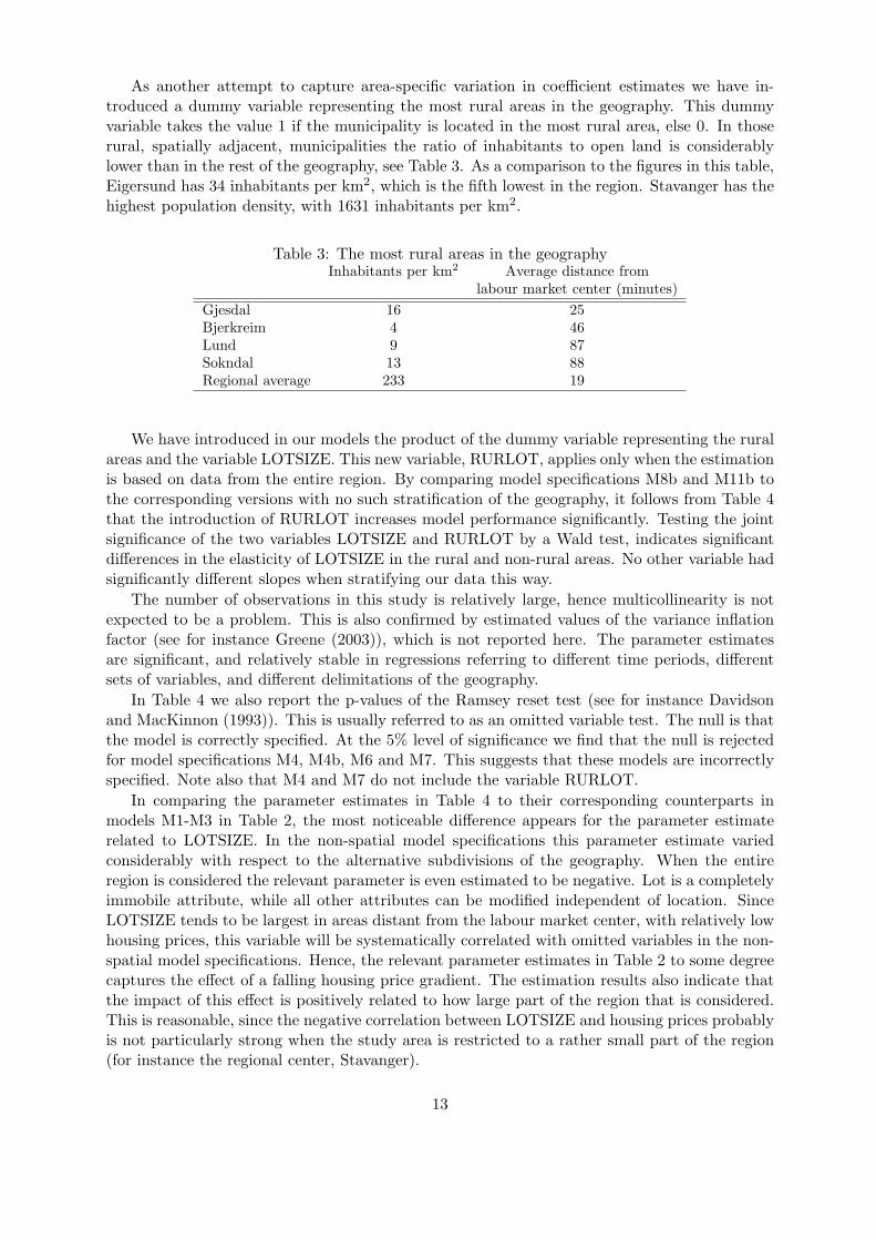
As another attempt to capture area-specific variation in coefficient estimates we have in-troduced a dummy variable representing the most rural areas in the geography. This dummyvariable takes the value 1 if the municipality is located in the most rural area, else 0. In thoserural, spatially adjacent, municipalities the ratio of inhabitants to open land is considerablylower than in the rest of the geography, see Table 3. As a comparison to the figures in this table,Eigersund has 34 inhabitants per km2, which is the fifth lowest in the region. Stavanger has thehighest population density, with 1631 inhabitants per km2.

Table 3: The most rural areas in the geographyInhabitants per km2 Average distance from

labour market center (minutes)Gjesdal 16 25Bjerkreim 4 46Lund 9 87Sokndal 13 88Regional average 233 19

We have introduced in our models the product of the dummy variable representing the ruralareas and the variable LOTSIZE. This new variable, RURLOT, applies only when the estimationis based on data from the entire region. By comparing model specifications M8b and M11b tothe corresponding versions with no such stratification of the geography, it follows from Table 4that the introduction of RURLOT increases model performance significantly. Testing the jointsignificance of the two variables LOTSIZE and RURLOT by a Wald test, indicates significantdifferences in the elasticity of LOTSIZE in the rural and non-rural areas. No other variable hadsignificantly different slopes when stratifying our data this way.

The number of observations in this study is relatively large, hence multicollinearity is notexpected to be a problem. This is also confirmed by estimated values of the variance inflationfactor (see for instance Greene (2003)), which is not reported here. The parameter estimatesare significant, and relatively stable in regressions referring to different time periods, differentsets of variables, and different delimitations of the geography.

In Table 4 we also report the p-values of the Ramsey reset test (see for instance Davidsonand MacKinnon (1993)). This is usually referred to as an omitted variable test. The null is thatthe model is correctly specified. At the 5% level of significance we find that the null is rejectedfor model specifications M4, M4b, M6 and M7. This suggests that these models are incorrectlyspecified. Note also that M4 and M7 do not include the variable RURLOT.

In comparing the parameter estimates in Table 4 to their corresponding counterparts inmodels M1-M3 in Table 2, the most noticeable difference appears for the parameter estimaterelated to LOTSIZE. In the non-spatial model specifications this parameter estimate variedconsiderably with respect to the alternative subdivisions of the geography. When the entireregion is considered the relevant parameter is even estimated to be negative. Lot is a completelyimmobile attribute, while all other attributes can be modified independent of location. SinceLOTSIZE tends to be largest in areas distant from the labour market center, with relatively lowhousing prices, this variable will be systematically correlated with omitted variables in the non-spatial model specifications. Hence, the relevant parameter estimates in Table 2 to some degreecaptures the effect of a falling housing price gradient. The estimation results also indicate thatthe impact of this effect is positively related to how large part of the region that is considered.This is reasonable, since the negative correlation between LOTSIZE and housing prices probablyis not particularly strong when the study area is restricted to a rather small part of the region(for instance the regional center, Stavanger).

13

Table 4: Results based on model specifications where spatial separation is measured by travelingtime from the labour market center of the geography

M4 M4b M5 M6 M7 M7b M8 M9

Constant 10,9235 10,8766 10,6641 10,51 12,15 12,09 11,87 11,66(0,0887) (0,0873) (0,1006) (0,1358) (0,0811) (0,0896) (0,1020) (0,1364)

LOTSIZE 0,1126 0,1181 0,1310 0,1371 0,1240 0,1319 0,1351 0,1338(0,0110) (0,0106) (0,0113) (0,0156) (0,0088) (0,0100) (0,0111) (0,0154)

RURLOT - -0,02914 - - - -0,0319 - -(-) (0,0033) (-) (-) (-) (0,0033) (-) (-)

AGE -0,0799 -0,0763 -0,0698 -0,0728 -0,0931 -0,0897 -0,0768 -0,0761(0,0066) (0,0065) (0,0072) (0,0087) (0,0048) (0,0065) (0,0073) (0,0084)

AGE·REBUILD 0,0106 0,01053 0,0113 0,01537 0,0109 0,0107 0,0116 0,0158(0,0028) (0,0030) (0,0032) (0,0041) (0,0028) (0,0030) (0,0032) (0,0041)

GARAGE 0,0683 0,0639 0,0414 0,02748 0,0749 0,0706 0,0479 0,0339(0,0113) (0,0110) (0,0119) (0,0161) (0,0104) (0,0111) (0,0120) (0,0160)

LIVAREA 0,3583 0,3558 0,3865 0,4190 0,3581 0,3553 0,3743 0,4107(0,0179) (0,0179) (0,0218) (0,0323) (0,0162) (0,0179) (0,0219) (0,0327)

NUMBTOIL 0,1515 0,1491 0,1351 0,1236 0,15933 0,1557 0,1421 0,1292(0,0151) (0,0147) (0,0167) (0,0227) (0,0142) (0,0148) (0,0167) (0,0228)

βe (exponential) -0,0256 -0,0218 -0,0254 -0,0303 - - - -(0,0013) (0,0015) (0,0018) (0,0047) (-) (-) (-) (-)

βp (power) - - - - -0,2363 -0,2198 -0,1794 -0,1500(-) (-) (-) (-) (0,0054) (0,0060) (0,0082) (0,0127)

YEARDUM97 -0,1352 -0,1343 -0,1302 -0,1551 -0,1342 -0,1332 -0,1307 -0,1557(0,0139) (0,0136) (0,0158) (0,0231) (0,0133) (0,0136) (0,0158) (0,0231)

YEARDUM99 0,1305 0,1261 0,1383 0,1466 0,1378 0,1329 0,1421 0,1437(0,0140) (0,0137) (0,01561) (0,0217) (0,0139) (0,0138) (0,0156) (0,0218)

YEARDUM00 0,2700 0,2678 0,2710 0,2627 0,2714 0,2690 0,2718 0,2624(0,0139) (0,0136) (0,0154) (0,0205) (0,0135) (0,0135) (0,0154) (0,0204)

YEARDUM01 0,3079 0,3019 0,3062 0,3027 0,3128 0,3065 0,3107 0,3008(0,0140) (0,0137) (0,0163) (0,0224) (0,0144) (0,0137) (0,0164) (0,0223)

n 2788 2788 2051 1188 2788 2788 2051 1188R2 0,7231 0,7350 0,6751 0,6910 0,7175 0,7319 0,6734 0,6949R2-adj. 0,7220 0,7339 0,6734 0,6881 0,7163 0,7308 0,6717 0,6920L 204,4133 266 257 112 176 249 252 120APE 221409 217571 234292 255226 227961 221501 235668 254110White test statistic 253 261 192 114 249 263 146 114Moran’s I 0,0271 0,0066 0,0061 0,0102 0,0431 0,0077 0,0037 0,0064Standard normal deviate (zI) 11,49 3,44 2,50 3,73 16,09 4,46 2,07 2,83Ramsey reset test (p-value) 0,0000 0,0001 0,3976 0,0056 0,0294 0,1523 0,68 0,47

Note: Results based on observations from the period 1997-2001, robust standard errors in parentheses. Models

M8-M10 are based on a negative exponential spatial separation function, M11-M13 are based on a power

function specification. The number of observations (n) indicates the relevant delimitation of the geography.

14

We will not enter into a detailed discussion of specific parameter estimates in Table 4.As a general comment there is a tendency that the introduction of distance results in moreprecise parameter estimates, and that the estimates are less dependent on what subdivision ofthe geography they refer to. Hence, it is important to account for an appropriate measure ofspatial separation to reach a satisfying identification of how partial variation in the independentvariables affects housing prices.

The introduction of distance from the labour market center in general improves the goodness-of-fit considerably. This especially applies for the case where the estimation is based on data fromthe entire region, with R2 (adjusted) increasing from 0,5120 (model M1) to around 0,73 (modelsM4b and M7b)). In the case where the study area is restricted to Stavanger the correspondingincrease only range from 0,6578 (M2) to around 0,67 (M6 and M9).

With reference to the trade-off theory it is natural that the contribution of distance inexplaining housing prices increases with the spatial extension of the study area within a labourmarked region. This pattern is reflected in the values of all the reported indicators of modelperformance in Table 4. Notice, however, that the introduction of distance significantly improvesmodel performance for all the reported subdivisions of the geography. In the case based on datafrom the entire region (comparing M7b to M1) the value of the likelihood ratio test statisticis 1658, which of course by far exceeds the critical value of a chi square distribution with twodegrees of freedom. When only Stavanger is considered (comparing M9 to M2) the value of thistest statistic is 126.

By comparing Table 2 and Table 4 it follows that the values of Moran’s I are considerablyreduced when a distance from the cbd is introduced in the model specifications. By comparingM4 to M4b and M7 to M7b it also follows that spatial autocorrelation is reduced when thevariable RURLOT is introduced. This clearly indicates that at least a large part of the spatialautocorrelation in the non-spatial modeling alternatives was due to the fact that importantinformation was omitted from the model specifications. RURLOT and, in particular, distancefrom the cbd represent characteristics of spatial structure that influence housing prices. Noticefrom Table 4, however, that the hypothesis of no spatial autocorrelation has to be rejected in allthe models M4-M9. Hence, the presence of autocorrelation is not removed, and the estimates offor instance R2 might still be artificially high.

6 Housing price gradients and alternative functional representa-tion of the relationship between housing prices and travelingtime

6.1 Comparing the exponential and the power function specification

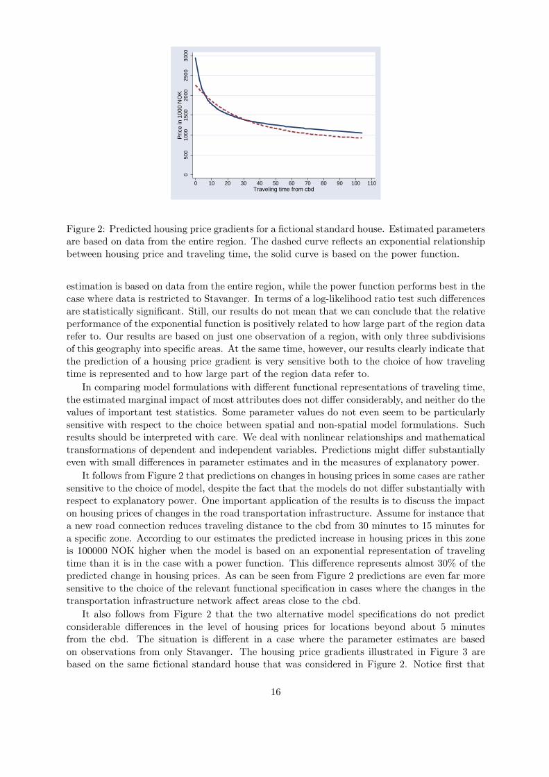
The two gradients in Figure 2 apply for a given set of values on all independent variables exceptthe traveling time from the cbd. We consider a fictional house that has not been rebuilt, andwith a garage. The fictional house is not located in the most rural areas, and the price in thefigure refers to year 2000. For the remaining independent variables we use observed averagevalues. Given this fixed set of values on attributes we predict housing prices in varying distancesfrom the cbd. The dashed curve refer to a path where spatial separation is represented by eβ̂edij ,

while the solid curve reflects the power function specification (dβ̂p

ij ). The parameter values arebased on models M4b and M7b, which means that β̂e = −0, 0218 and β̂p = −0, 2198.

In general it follows from the results in Table 4 that the two alternative functions of travelingtime only result in marginal differences in explanatory power. For all the measures of explanatorypower a tendency can be found, however, that the exponential function performs best when the

15

050

010

0015

0020

0025

0030

00P

rice

in 1

000

NO

K0 10 20 30 40 50 60 70 80 90 100 110

Traveling time from cbd

Figure 2: Predicted housing price gradients for a fictional standard house. Estimated parametersare based on data from the entire region. The dashed curve reflects an exponential relationshipbetween housing price and traveling time, the solid curve is based on the power function.

estimation is based on data from the entire region, while the power function performs best in thecase where data is restricted to Stavanger. In terms of a log-likelihood ratio test such differencesare statistically significant. Still, our results do not mean that we can conclude that the relativeperformance of the exponential function is positively related to how large part of the region datarefer to. Our results are based on just one observation of a region, with only three subdivisionsof this geography into specific areas. At the same time, however, our results clearly indicate thatthe prediction of a housing price gradient is very sensitive both to the choice of how travelingtime is represented and to how large part of the region data refer to.

In comparing model formulations with different functional representations of traveling time,the estimated marginal impact of most attributes does not differ considerably, and neither do thevalues of important test statistics. Some parameter values do not even seem to be particularlysensitive with respect to the choice between spatial and non-spatial model formulations. Suchresults should be interpreted with care. We deal with nonlinear relationships and mathematicaltransformations of dependent and independent variables. Predictions might differ substantiallyeven with small differences in parameter estimates and in the measures of explanatory power.

It follows from Figure 2 that predictions on changes in housing prices in some cases are rathersensitive to the choice of model, despite the fact that the models do not differ substantially withrespect to explanatory power. One important application of the results is to discuss the impacton housing prices of changes in the road transportation infrastructure. Assume for instance thata new road connection reduces traveling distance to the cbd from 30 minutes to 15 minutes fora specific zone. According to our estimates the predicted increase in housing prices in this zoneis 100000 NOK higher when the model is based on an exponential representation of travelingtime than it is in the case with a power function. This difference represents almost 30% of thepredicted change in housing prices. As can be seen from Figure 2 predictions are even far moresensitive to the choice of the relevant functional specification in cases where the changes in thetransportation infrastructure network affect areas close to the cbd.

It also follows from Figure 2 that the two alternative model specifications do not predictconsiderable differences in the level of housing prices for locations beyond about 5 minutesfrom the cbd. The situation is different in a case where the parameter estimates are basedon observations from only Stavanger. The housing price gradients illustrated in Figure 3 arebased on the same fictional standard house that was considered in Figure 2. Notice first that

16

a predicted housing price in a long distance from the cbd is now a lot more sensitive to thechoice of a functional representation of traveling time than in the case where estimation is basedon observations from the entire region. This illustrates the trivial but important point thatidentification of such a relationship is positively related to the deviation in observed values ofthe independent variable. Hence, a predicted housing price gradient is in general more reliable ifit is based on observations covering a wide range of values on traveling time from the cbd. Ourstudy area is very appropriate for this purpose, since the local housing market only marginallyinterferes with housing markets in adjacent areas outside the region. The region can in thisrespect be considered as an isolated island with one dominating central place.

Another point to notice is that the sensitivity of the housing prices with respect to variationsin short distances from the cbd changes considerably for both model specifications if only datafrom Stavanger are used in the estimation procedure. It is reasonable that the two alternativemodel specifications predict very similar housing prices for distances within 15 minutes from thecbd in a case where the estimation is primarily based on data for such values of distance. Atthe same time those results also contribute to an evaluation of the two alternative housing pricegradients in Figure 2, with data based on observations from the entire region. To be specific,the results clearly indicate that the power function approach gives a considerably biased slopeof the housing price gradient for low values of traveling time from the cbd. This conclusion alsocorresponds to a combination of intuition and knowledge of the local geography. Hence, gradientsbased on the power function seem to predict too radical changes in housing prices for variationsin distances close to the cbd. With data based on the entire geography the exponential functionresults in a more reasonable housing price gradient for this rather monocentric geography.

050

010

0015

0020

0025

0030

00P

rice

in 1

000

NO

K

0 10 20 30 40 50 60 70 80 90 100 110Traveling time from cbd

Figure 3: Predicted housing price gradients for a fictional standard house. Estimated parametersare based on data from Stavanger. The dashed curve reflects an exponential relationship betweenhousing price and traveling time, the solid curve is based on the power function.

Housing price gradients can be stated in terms of physical distance rather than traveling time.In such cases the graph will not in general be autonomous to changes in road transportationinfrastructure. An innovation in the road network might for instance result in reduced travelingtime even if the physical distance is unaffected. This can be due to higher speed limits and/orimproved road standard. In such a case a housing price gradient expressed in terms of physicaldistance will shift to the right, and the slope will be reduced. With traveling time representedon the horizontal axis predictions follow directly from movements along the curve.

17

6.2 More complex specifications of the relationship between housing pricesand traveling time

It follows from the discussion in the previous subsection that an empirically based evaluationof distribution and capitalization effects of investments in road transportation infrastructureis rather sensitive to the functional specification of spatial separation in the model. Thereare of course many specifications alternative to the exponential and the power function. Onealternative is a logistic function, where traveling time enters through the following expression:

f(dij) =β0

1 + eβ1+β2·dij

Another alternative is the conventional Box-Cox transformation. This transformation isexpressed through the specification of the variable Zij , defined by:

Zij =dλ

ij − 1λ

In Table 5 we let βz represent the marginal impact of changes in Zij on housing prices. Inprinciple a procedure where λ is estimated allows for a more flexible way to take the effectof traveling time into account. It is not a priori obvious that spatial separation should berepresented by either dij or ln dij in the relevant relationship. As in the previous subsection weassume a log-linear relationship between the dependent and the remaining independent variables.In the estimation intrazonal distances of zero are substituted by arbitrarily small numbers.

To summarize, we consider the following alternative model specifications:

M10: traveling time is represented through a logistic function

M11: traveling time enters through a Box-Cox transformation

Results are presented in Table 5. All results in this table are based on data from the entiremodel. Compare first M10 to M4b. It then follows that the model formulation based on alogistic function adds significantly to the explanatory power, since the value of the likelihoodratio test statistic is approximately 9, which exceeds the critical value of a chi square distributionwith two degrees of freedom. It also follows from Table 5 that the Box-Cox specification addseven more to explanatory power, with only one parameter more than the exponential distancedeterrence function in M4b.

This means that the explanatory power is significantly improved as a result of the conven-tional Box-Cox transformation. One objection against this approach concerns the interpretationof the transformation parameter λ. In a case with heteroskedasticity it is well known (see forinstance Kmenta (1983)) that the estimate of this parameter will almost certainly be less than 1,it is biased towards zero. The Box-Cox transformation adjusts both for heteroskedasticity andfor an incorrect functional form. Low values of λ reduce heteroskedasticity in residuals. Hence,we cannot be sure that our parameter estimate defines an appropriate functional form of spatialseparation in the model. This also means that the resulting housing price gradient is biased.

Rather than a Box-Cox transformation Kmenta (1983) recommends a spline-function ap-proach to test for nonlinearity. Such an approach has been used for instance by Dubin andSung (1987), for the estimation of housing rent gradients in non-monocentric cities. We assumea function that is piecewise log-linear, and introduce two knots, defining three segments of thehousing price gradient. At the outset a component-plus-residual plot (Ezekiel 1924, Larsen andMcCleary 1972) was used to detect nonlinearity. The locations of the knots were then determinedthrough a search procedure, identifying the values that were maximizing the explanatory power

18

of the regression model. We let the spline function with two knots (d1ij and d2

ij) be representedby the following specification of the relevant function:

g0(dij) = dβ0+δ

(1)ij β1+δ

(2)ij β2

ij

Here, δ(1)ij and δ

(2)ij are Kronecker deltas, defined by:

δ(k)ij =

{1 if dij > dk

ij k = 1, 20 otherwise

With such a parametric specification β1 and β2 can be interpreted as discontinuous correctionsin the effects of variations in traveling time by moving from one segment to the next, and thespecification refers to model M12 in Table 5:

M12: traveling time is represented by a piecewise log-linear spline function with two knots

Since this spline function enters into a log-linear relationship, the elasticity of housing price withrespect to distance is constant within each of the three segments of the gradient. According tothe results in Table 5 there is a significant discontinuous change in housing prices at a distancecorresponding to 20 minutes of traveling time from the cbd. The relevant elasticity increasesfrom -0,1649 to -0,3527 when traveling time exceeds 20 minutes. A natural hypothesis is thatthis reflects a discontinuous change in commuting behavior at such distances. The second knotthat is reported in Table 5 appears for a traveling time of 55 minutes from the cbd. The segmentrepresented by traveling times exceeding 55 minutes has an elasticity of -0,1539. The parameterrelated to this knot is not, however, significant at the 5% level.

According to the log-likelihood ratio test this spline function model specification fits datasignificantly better than the Box-Cox modeling approach. The value of the likelihood ratio teststatistic is 7.3, which exceeds the critical value at the 5 % significant level.

We have also tested a model specification where the distance function entering into thehedonic regression model is assumed to be piecewise linear:

M13: traveling time is represented by a piecewise linear spline function with three knots

This model specification does of course not imply that the housing price gradient is piecewiselinear, since the distance function appears in an equation where the dependent variable appearsthrough its natural logarithm. Based on the component-plus-residual plot we found it naturalto specify three knots (d1

ij , d2ij , and d3

ij) at the outset. The distance deterrence relationship isthen represented by the following expression in the model:

g1(dij) = (β0 + δ(1)ij β1 + δ

(2)ij β2 + δ

(3)ij β3)dij

Once again:

δ(k)ij =

{1 if dij > dk

ij k = 1, 2, 30 otherwise

This estimation resulted in the following three knots: δ(1)ij = 5, δ

(2)ij = 21, and δ

(3)ij = 55.

The two versions of the spline function are illustrated in Figure 4. In both cases we predictonly marginal reductions in housing prices when traveling time increases beyond 55 minutes.For all practical purposes the two curves are more or less totally overlapping. According tolog-likelihood values reported in Table 5 the approach where traveling time appears through apiecewise linear function results in a significantly higher explanatory power than all the alter-native model specifications.

19

050

010

0015

0020

0025

0030

00P

rice

in 0

00 N

OK

0 10 20 30 40 50 60 70 80 90 100 110Traveling time from cbd

M12

050

010

0015

0020

0025

0030

00P

rice

in 0

00 N

OK

0 10 20 30 40 50 60 70 80 90 100 110Traveling time from cbd

M13

Figure 4: Predicted housing price gradients for a fictional standard house. The left part of thefigure represents model M12, the right part is based on model M13.

Objections can be raised against the data-driven spline function approach. One such objec-tion is that very close neighbors on either side of a knot is implicitly assigned distinctly differentdistance responsiveness in commuting demand. Another kind of arbitrariness concerns the num-ber of knots. In general explanatory power is positively related to the number of knots. At thelimit a specification can be chosen where workers with the same number of minutes travelingtime from the cbd are assigned a specific distance responsiveness. Such an approach probablyfits well to the observations, but it does definitely not represent a satisfying general hypothesisof commuting behavior. Hence, it also at best represents a questionable basis for predictingeffects of changes in for example road transportation infrastructure.

In the previous subsection we concluded that a model specification based on an exponentialrepresentation of traveling time is superior to an approach based on a power function. One reasonfor this was that the power function results in a housing price gradient where housing prices areunreasonably sensitive to variations in short distances from the cbd. This tentative conclusionwas supported by the results following from the spline function approach considered above.Hence, both intuition and numerical results indicate that the assumption of a globally constantelasticity of housing prices with respect to distance does not provide a satisfying explanationof our observations. As an alternative to the spline function approach this can be adjusted forby introducing a quadratic term in the regression equation. Traveling time then appears in theregression equation through the following expression:

h(dij) = dβij · ((dij)2)βq

This corresponds to model specification M14 in Table 5:

M14: the power function is supplemented by a quadratic term

With such a specification the elasticity of housing price with respect to distance is:

EldijPi = Eldij

h(dij) = β + 2βq ln dij

Notice first from Table 5 that both parameters related to distance are significantly negative;β̂ = −0, 0689 and β̂q = −0, 0295. This means that housing prices become increasingly moreelastic with respect to distance for movements downwards along the housing price gradient.The point elasticity is −0, 0689 when the traveling time is 1 minute from the cbd, while it is forinstance −0, 2048 and −0, 2997 for locations with respectively 10 and 50 minutes of travelingtime to the cbd.

20

Compared to the pure power function specification (M7b) the quadratic term adds signifi-cantly to the explanatory power. Model M14 also fits data significantly better than the approachbased on an exponential distance deterrence function, M4b; the value of the relevant likelihoodratio test statistic is about 14. Evaluated from the measures of model performance reported inTable 5 it is not possible to distinguish significantly between the quadratic approach and theBox-Cox approach.

We have seen that the alternative, somewhat more complex, functions contribute signifi-cantly to the explanatory power compared to a simple exponential function. For most practicalpurposes, however, this difference in explanatory power probably does not matter very much.From a practical point of view criteria related to predictability of housing price gradients rep-resent a more important basis for the choice of a model specification. Such criteria are difficultto formulate in an empirical context. Physically more or less identical houses probably can befound at different locations, but prices are also influenced by variation in local aspects that wehave not incorporated into the model. Hence, the choice of a model specification has to be basedon more tentative considerations, and/or sensitivity analysis.

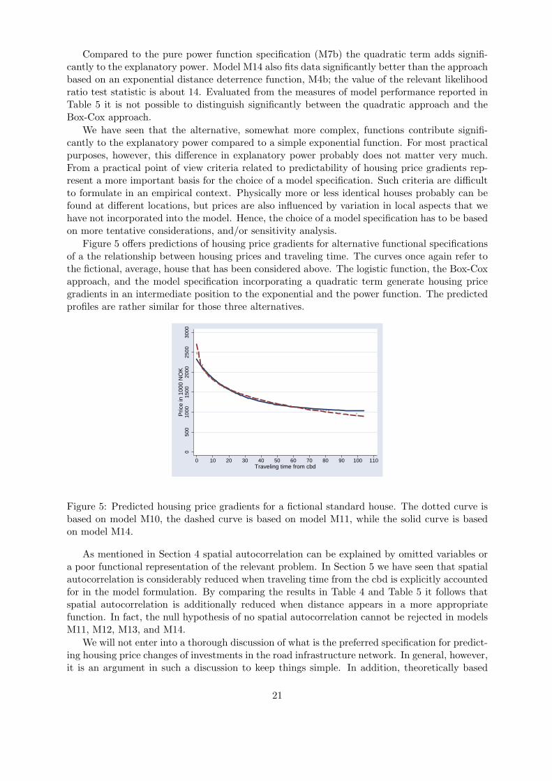
Figure 5 offers predictions of housing price gradients for alternative functional specificationsof a the relationship between housing prices and traveling time. The curves once again refer tothe fictional, average, house that has been considered above. The logistic function, the Box-Coxapproach, and the model specification incorporating a quadratic term generate housing pricegradients in an intermediate position to the exponential and the power function. The predictedprofiles are rather similar for those three alternatives.

050

010

0015

0020

0025

0030

00P

rice

in 1

000

NO

K

0 10 20 30 40 50 60 70 80 90 100 110Traveling time from cbd

Figure 5: Predicted housing price gradients for a fictional standard house. The dotted curve isbased on model M10, the dashed curve is based on model M11, while the solid curve is basedon model M14.

As mentioned in Section 4 spatial autocorrelation can be explained by omitted variables ora poor functional representation of the relevant problem. In Section 5 we have seen that spatialautocorrelation is considerably reduced when traveling time from the cbd is explicitly accountedfor in the model formulation. By comparing the results in Table 4 and Table 5 it follows thatspatial autocorrelation is additionally reduced when distance appears in a more appropriatefunction. In fact, the null hypothesis of no spatial autocorrelation cannot be rejected in modelsM11, M12, M13, and M14.

We will not enter into a thorough discussion of what is the preferred specification for predict-ing housing price changes of investments in the road infrastructure network. In general, however,it is an argument in such a discussion to keep things simple. In addition, theoretically based

21

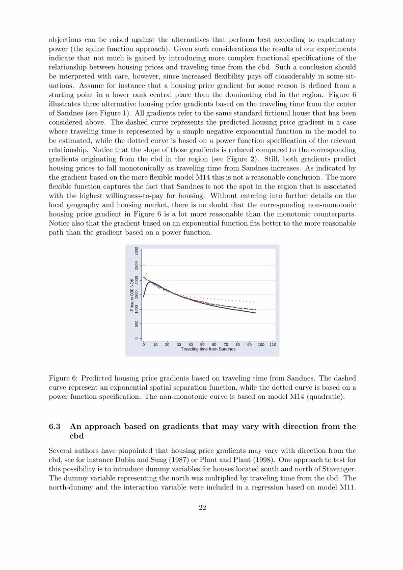
objections can be raised against the alternatives that perform best according to explanatorypower (the spline function approach). Given such considerations the results of our experimentsindicate that not much is gained by introducing more complex functional specifications of therelationship between housing prices and traveling time from the cbd. Such a conclusion shouldbe interpreted with care, however, since increased flexibility pays off considerably in some sit-uations. Assume for instance that a housing price gradient for some reason is defined from astarting point in a lower rank central place than the dominating cbd in the region. Figure 6illustrates three alternative housing price gradients based on the traveling time from the centerof Sandnes (see Figure 1). All gradients refer to the same standard fictional house that has beenconsidered above. The dashed curve represents the predicted housing price gradient in a casewhere traveling time is represented by a simple negative exponential function in the model tobe estimated, while the dotted curve is based on a power function specification of the relevantrelationship. Notice that the slope of those gradients is reduced compared to the correspondinggradients originating from the cbd in the region (see Figure 2). Still, both gradients predicthousing prices to fall monotonically as traveling time from Sandnes increases. As indicated bythe gradient based on the more flexible model M14 this is not a reasonable conclusion. The moreflexible function captures the fact that Sandnes is not the spot in the region that is associatedwith the highest willingness-to-pay for housing. Without entering into further details on thelocal geography and housing market, there is no doubt that the corresponding non-monotonichousing price gradient in Figure 6 is a lot more reasonable than the monotonic counterparts.Notice also that the gradient based on an exponential function fits better to the more reasonablepath than the gradient based on a power function.

050

010

0015

0020

0025

0030

00P

rice

in 0

00 N

OK

0 10 20 30 40 50 60 70 80 90 100 110Traveling time from Sandnes

Figure 6: Predicted housing price gradients based on traveling time from Sandnes. The dashedcurve represent an exponential spatial separation function, while the dotted curve is based on apower function specification. The non-monotonic curve is based on model M14 (quadratic).

6.3 An approach based on gradients that may vary with direction from thecbd

Several authors have pinpointed that housing price gradients may vary with direction from thecbd, see for instance Dubin and Sung (1987) or Plaut and Plaut (1998). One approach to test forthis possibility is to introduce dummy variables for houses located south and north of Stavanger.The dummy variable representing the north was multiplied by traveling time from the cbd. Thenorth-dummy and the interaction variable were included in a regression based on model M11.

22

Table 5: Results based on alternative specifications of spatial separation and spatial structureM14 M15 M16 M17 M18

Constant 11,0262 11,9378 12,0408 12,0342 11,9275(0,0878) (0,0878) (0,0881) (0,0939) (0,0810)

LOTSIZE 0,1203 0,1172 0,1224 0,1225 0,1262(0,0103) (0,0098) (0,0102) (0,0101) (0,0085)

RURLOT -0,0303 -0,0303 -0,0326 -0,0311 -0,0300(0,0032) (0,0032) (0,0031) (0,0032) (0,0026)

AGE - 0,0784 - 0,0805 - 0,0826 -0,0824 - 0,0828(0,0064) (0,0063) (0,0065) (0,0066) (0,0048)

AGE·REBUILD 0,0105 0,0109 0,017 0,0107 0,0106(0,0029) (0,0027) (0,0029) (0,0029) (0,0027)

GARAGE 0,0661 0,0654 0,0677 0,0679 0,0670(0,0109) (0,0110) (0,0110) (0,0110) (0,0101)

LIVAREA 0,3593 0,3538 0,3517 0,3514 0,3573(0,0178) (0,0178) (0,0178) (0,0178) (0,0157)

NUMBTOIL 0,1495 0,1546 0,1522 0,1518 0,1522(0,0147) (0,0147) (0,0146) (0,0147) (0,0137)

β0 (logistic) 3820,666 - - - -(8,5879) (-) (-) (-) (-)

β1 (logistic) 8,4126 - - - -(0,0399) (-) (-) (-) (-)

β2 (logistic) 0,0313 - - - -(0,0034) (-) (-) (-) (-)

βz (Box-Cox) - - 0,0641 - -(-) (0,0017) (-) (-) (-)

λ (Box-Cox) - 0,4313 - - -(-) (0,0251) (-) (-)

β0 (spline, power) - - -0,1649 -(-) (-) (0,0086) (-)

β1 (spline, power) - - -0,1878 -(-) (-) (0,0263) (-) (-)

β2 (spline, power) - - 0,1988 - -(-) (-) (0,1278) (-) (-)

β0 (spline, linear) - - - -0,0557 -(-) (-) (-) (0,0060) (-)

β1 (spline, linear) - - - 0,0395 -(-) (-) (-) (0,0064) (-)

β2 (spline, linear) - - - 0,0067 -(-) (-) (-) (0,0016) (-)

β3 (spline, linear) - - - 0,0078 -(-) (-) (-) (0,0025) (-)

β (quadratic) - - - - - 0,0689(-) (-) (-) (-) (0,0202)

βq (quadratic) - - - - - 0,0295(-) (-) (-) (-) (0,0038)

YEARDUM97 -0,1336 -0,1346 -0,1350 -0,1348 - 0,1333(0,0135) (0,0135) (0,0135) (0,0135) (0,0128)

YEARDUM99 0,1275 0,1288 0,1289 0,1288 0,1295(0,0137) (0,0137) (0,0137) (0,0137) (0,0134)

YEARDUM00 0,2684 0,2672 0,2684 0,2686 0,2686(0,0135) (0,0136) (0,0135) (0,0135) (0,0130)

YEARDUM01 0,3031 0,3024 0,3045 0,3044 0,3041(0,0136) (0,0137) (0,0137) (0,0136) (0,0139)

n 2788 2788 2788 2788 2788R2 0,7368 0,7378 0,7385 0,7396 0,7376R2-adj. 0,7356 0,7367 0,7372 0,7382 0,7364L 275,4067 280,78 284,4316 290,4447 279,68APE 217020,33 216901,08 216921,28 216222,25 216736,08White test statistic 252 255 288 306 264Moran’s I 0,0036 0,0019 0,0012 0,0010 0,0015Standard normal deviate (zI) 2,3151 1,4027 1,1896 1,1255 1,3068Ramsey reset test (p-value) 0,4241 0,7860 0,9280 0,8853 0,8274

Note: Results based on observations from the period 1997-2001, robust standard errors in parentheses.

23

The number of observations is 118 in the north, and 2670 in the south; the region only rangesover 24 minutes in the northern direction. The two new coefficients got robust t-values of about2,3. A Wald test was performed, testing the null hypothesis of equality between the generalcoefficient representing traveling time, and the coefficient representing traveling times towardthe north. This null hypothesis could not be rejected. Hence, the price distance gradient is notconsidered to be statistically different in the north and in the south of the cbd. Once again, thisis an indication that the area we consider is fairly homogenous.

7 Concluding remarks

In this paper we have studied the impact of spatial and non-spatial variables on housing pricesin the southernmost region in Western Norway. We have primarily focused on the impact ofspatial separation on housing prices, and on the form of housing price gradients correspondingto a specific set of other attributes. The region has one dominating center (Stavanger), andthe diffusion of new residential areas has to a large degree been determined by employmentgrowth in, and close to, this center. This is one reason why the region is very appropriate forthe purpose of identifying reliable housing price gradients, reflecting to a relatively large degreehousing market equilibrium forces rather than characteristics of more complex multicentric andmultinodal systems.

We started out by considering non-spatial modeling alternatives, primarily representing abenchmark for evaluating more satisfying model specifications. The introduction of spatialseparation measures results in more precise parameter estimates and improved explanatorypower, especially in a case where the estimation is based on data from the entire region. Wehave evaluated alternative functional specifications of spatial separation in the hedonic modelformulation. Our main findings are:

• Our results indicate that predicted housing price gradients are in general not reliable ifestimation is based on observations covering only a part of the relevant labor and housingmarket originating from the cbd. This represents one possible reason why some studiesreport intuitively strange gradients.

• According to our results a power function specification of traveling time is not an appro-priate approach to predict housing price gradients. A log-linear regression model resultsin biased gradients, and tends to over-predict housing prices in locations close to thecbd. The exponential function performs better, and results in more reliable gradients inthe case where estimation is based on observations from the entire labor/housing market.Predicted housing prices might differ substantially even if values of estimated parametersand explanatory power are similar.

• The use of more complex and flexible functional specifications of traveling time contributessignificantly to the explanatory power compared to a one-parameter approach. For mostpractical purposes the difference in explanatory power does not matter very much. Themore flexible approaches lead to housing price gradients in an intermediate position be-tween the one-parameter exponential and power function approaches, and they probablyrepresent a more reliable basis for predictions.

• Our results do not distinguish clearly between the alternative flexible function approachesthat we have considered. Results on explanatory power should be considered in com-bination with pragmatic, theoretical and interpretational arguments. Based on such aconsideration we especially find the approach incorporating a quadratic term appealing.

24

In this kind of empirical research it is important to consider potential econometric problems.In particular one such potential problem is related to spatial autocorrelation. We find severespatial autocorrelation in models where no measure of spatial separation is accounted for. Alarge part of this autocorrelation is removed when traveling time is introduced through a one-parameter function. Autocorrelation is further reduced in the model formulations based onmore flexible functions. In the more flexible approaches we find that the hypothesis of no spatialautocorrelation cannot be rejected. Our results also indicate that increased functional flexibilitypays off in terms of more reliable predictions of housing price gradients if the geography is moremulticentric and/or multinodal than the one we consider, with less obvious identification of aregional center.

All in all we achieve encouraging results, with satisfying goodness-to-fit, reliable coefficientestimates, and intuitively reasonable predictions of housing price gradients. Our results repre-sent important input in an evaluation of for instance residential construction programs, urbanrenewal, and/or investments in transportation infrastructure. In addition our results contributeto a discussion of how forces relating to the housing market can be incorporated into a generalspatial equilibrium framework constructed for a region with one dominating center.

25

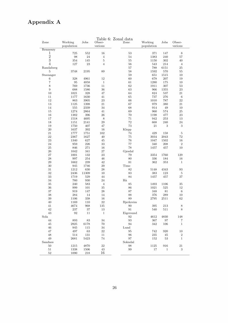
Appendix A

Table 6: Zonal dataZone Working Jobs Obser- Zone Working Jobs Obser-

population vations population vationsRennesøy

1 725 552 16 53 371 147 82 98 24 4 54 1383 240 573 354 145 5 55 1150 302 404 127 23 4 56 543 214 4

Randaberg 57 788 6151 255 3748 2195 89 58 1592 570 55

Stavanger 59 651 1515 106 328 4961 12 60 678 207 197 95 4058 1 61 1280 175 108 769 1736 11 62 1911 307 539 688 1586 36 63 966 1355 2310 1021 328 47 64 824 537 2111 1177 1630 41 65 737 276 612 863 3905 23 66 1010 787 2213 1125 1398 21 67 979 380 2114 555 2339 34 68 914 49 1015 1274 2864 41 69 960 574 2516 1382 396 26 70 1198 477 2317 1518 4695 8 71 942 253 1318 1151 2141 29 72 668 240 2419 1750 407 47 73 21 3 320 1637 392 16 Klepp21 1777 1751 102 74 429 158 522 2367 1627 40 75 3034 2043 7223 1340 627 45 76 1047 1502 1624 959 226 33 77 340 208 225 846 271 16 78 1457 457 1026 1042 341 27 Gjesdal27 1001 132 23 79 3354 1760 12928 997 254 46 80 336 184 1629 1662 239 42 81 362 353 130 945 1746 29 Time31 1212 630 28 82 5148 4343 9332 2436 11309 10 83 383 123 533 1719 529 44 84 1457 457 2734 760 930 24 H̊a35 240 583 4 85 1493 1106 3536 999 101 35 86 1021 525 1237 919 147 28 87 348 81 638 284 14 14 88 376 289 1039 1106 338 16 89 2795 2511 6240 1169 110 22 Bjerkreim41 4674 968 135 90 395 213 842 237 37 13 91 540 511 843 92 11 1 Eigersund

Sola 92 4612 4830 14844 893 83 34 93 367 97 745 2925 6178 70 94 342 106 146 945 115 34 Lund47 497 63 22 95 742 920 1048 514 131 11 96 235 45 249 2681 5423 74 97 152 53 1

Sandnes Sokndal50 1215 4870 22 98 1125 916 2151 1338 1506 43 99 17 1 352 1090 218 16

26

Appendix B

Table 7: Descriptive housing market statisticsOBSERVATIONS MEAN STD. DEV. MINIMUM MAXIMUM

STAVANGERREALPRICE 1188 1751240 662891 160000 4747500Price pr square meter 1192 10902 3335 1778 34451LIVAREA 1188 167 61 43 500LOTSIZE 1188 512 334 40 5243GARAGE 1188 0,68 0,47 0 1NUMBTOIL 1188 2 0,84 1 6AGE 1188 41 37 0 187REBUILD 1188 0,42 0,50 0 1TIMECBD 1188 6,58 3,2 0 25,8

RANDABERG, SOLA, AND SANDNESREALPRICE 863 1582665 518372 353425 4401000Price pr square meter 863 9386 3040 1767 24265LIVAREA 863 178 60 47 387LOTSIZE 863 679 346 80 4070GARAGE 863 0,79 0,41 0 1NUMBTOIL 863 2 0,81 1 6AGE 863 22 18 0 116REBUILD 863 0,33 0.47 0 1TIMECBD 863 16,1 6,2 6,2 57,3

MUNICIPALITIES IN THE REST OF THE REGIONREALPRICE 737 1100264 419500 204600 3892950Price pr square meter 737 7631 2696 897 22827LIVAREA 737 151 54 37 361LOTSIZE 737 728 326 37 2487GARAGE 737 0,74 0,44 0 1NUMBTOIL 737 2 0,72 0 6AGE 737 26 26 0 163REBUILD 737 0,31 0,46 0 1TIMECBD 737 48 20 21 220

THE ENTIRE REGIONREALPRICE 2788 1526976 622323 160000 4747500Price pr square meter 2788 9567 3358 896 33451LIVAREA 2788 166 60 37 500LOTSIZE 2788 621 349 37 5243GARAGE 2788 0,73 0,44 0 1NUMBTOIL 2788 2 0,81 0 6AGE 2788 31 30 0 220REBUILD 2788 0,36 0,48 0 1TIMECBD 2788 19 18 0 104

Note: Prices are measured in NOK, they have been adjusted for inflation, and 1998 represents the baseyear. LIVAREA and LOTSIZE are measured in square metres, and is measured TIMECBD in minutes.

27

References

[1] Adair A, S McGreal, A Smyth, J Cooper, and T Ryley, 2000, “House prices and accessibility:the testing of Relationships within the Belfast urban area”, Housing studies, 15 699-716.

[2] Alonso W, 1964, Location and land use. Toward a general theory of land, Harvard UniversityPress, Cambridge, Massachusetts.

[3] Anselin L, 1988, Spatial econometrics: methods and models. Kluwer Academic Publishers,London.

[4] Anselin L and Rey S, 1991, “Properties of tests for spatial dependence in linear regressionmodels”, Geographical Analysis 23, 113-131.

[5] Ball M J, 1973, ”Recent empirical work on the determinants of relative house prices”. UrbanStudies 10 213-233.

[6] Ball M J and R M Kirwan, 1977, “Accessibility and supply constraints in the urban housingmarket”, Urban studies 14 11-32.

[7] Barkley, D L, Henry M S, Bao S, Brooks K R, 1995, “How functional are economic areas?Tests for intra-regional spatial association using spatial data analysis,” Papers in RegionalScience 74 297-316.

[8] Bartik T J and V K Smith, 1987, Urban Amenities and public policy, Handbook of Regionaland Urban Economics, vol 2, Elsevier science publisher B.V, Netherlands.

[9] Brueckner J, 1987, The structure of urban equilibria: a unified treatment of the Muth-Millsmodel, Handbook of Regional and Urban Economics, vol 2, Elsevier science publisher B.V,Netherlands.

[10] Davidson R and J G MacKinnon, 1993, Estimation and Inference in Econometrics, OxfordUniversity Press. New York.

[11] Dubin, R A and C H Sung, 1987, ”Spatial variation in the price of housing rent gradientsin non-monocentric cities”, Urban Studies 24, 193-204.

[12] Dubin R A, 1992: “Spatial autocorrelation and neighbourhood quality”, Regional Scienceand Urban Economics 22 433-452.

[13] Ezekiel, M, 1924, ”A method of handling curvilinear correlation for any number of variables”Journal of the American Statistical Association 19, 431-453.

[14] Fik, T J and G F Mulligan, 1998, “Functional form and spatial interaction models”, Envi-ronment and Planning, volume 30, 1497-1507.

[15] Florax R J G M, Voortman R L and Brouwer J, 2002, “Spatial dimensions of precision agri-culture: a spatial econometric analysis of millet yield on Sahelian coversands”, AgriculturalEconomics, 27, 425-443.

[16] Greene W H, 2003, Econometric Analysis, Fifth edition, Prentice Hall.

[17] Hansen W G, 1959, “How accessibility shapes land use”, Journal of the American Instituteof Planners 25 73-76.

28

[18] Heikkela E, P Gordon, J I Kim, R B Peiser, H W Richardson, 1989, “What happened tothe CBD-distance gradient?: land values in a polycentric city”, Environment and PlanningA 21 221-232.

[19] Kmenta J, 1986, Elements of Econometrics, Macmillan, New York.

[20] Laakso S, 1997, “Urban housing prices and the demand for housing characteristics. A studyon housing prices and the willingness to pay for housing characteristics and local publicgoods in the Helsinki Metropolitan Area”, The research Institute of the Finnish Economy,Helsinki.

[21] Larsen, W A and S J McCleary, 1972 ”The use of partial residual plots in regressionanalysis”, Technometrics 14, 781-790.

[22] Mills E, 1967, ”An aggregated model of resource allocation in a metropolitan area”, Amer-ican Economic Review 57 197-210.

[23] Muth R F, 1969, Cities and housing, University of Chicago Press.

[24] Nijkamp, P. and A. Reggiani. 1992. Interaction, evolution and chaos in space, Springer-Verlag

[25] Odland, J, 1988, Spatial autocorrelation, Sage Publicationd Inc.

[26] Plaut P O and S E Plaut, 1998, “Endogenous identification of multiple housing price centersin metropolitan areas”, Journal of Housing Economics 7 193-217.

[27] Rosen S, 1974, “Hedonic prices and implicit markets: product differentiation in pure com-petition”, Journal of Political Economy 82 34-55.

[28] Rothenberg J, G C Galster, R V Butler, and J Pitkin, (1991), The maze of urban markets.Theory, evidence and policy, University of Chicago Press.

[29] Sheppard S, 1999, “Hedonic analysis of housing markets”, Handbook of Regional and UrbanEconomics, ed. by E S Mills and P Chesire.

[30] Strazheim M R, 1974, ”Hedonic estimation of housing market prices. A further comment”The Review of Economics and Statistics 56 404-406.

[31] Thorsen I, Gitlesen J P, 1998, “Empirical evaluation of alternative model specifications topredict commuting flows”, Journal of Regional Science, 38 273-292

[32] Waddell P, Berry B J L, and I Hock, 1993, “Residential Property Values in a Multinodal Ur-ban Area: New Evidence of the Implicit Price of Location” Journal of Real Estate Financeand Economics 7 117-141.

[33] Whitehead C M E, 1999, “Urban housing markets: theory and policy”, Handbook of Re-gional and Urban Economics, ed. by E S Mills and P Chesire.

29

Department of EconomicsUniversity of BergenFosswinckels gate 6N-5007 Bergen, NorwayPhone: +47 55 58 92 00Telefax: +47 55 58 92 10http://www.svf.uib.no/econ