Amphibian species richness across environmental gradients

Earl E. Werner, David K. Skelly, Rick A. Relyea and Kerry L. Yurewicz

E. E. Werner (eewerner@umich.edu), Dept of Ecology and Evolutionary Biology, Univ. of Michigan, Ann Arbor, MI 48109, USA. �D. K. Skelly, School of Forestry & Environmental Studies, Yale Univ., New Haven, CT 06511, USA. � R. A. Relyea, Dept ofBiological Sciences, Univ. of Pittsburgh, Pittsburgh, PA 15260, USDA. � K. L. Yurewicz, Biological Sciences, Plymouth State Univ.,Plymouth, NH 03264, USA.

Large-scale field patterns are a fundamental source of inferences on processes responsible for variation in speciesrichness among habitats. We examined species richness of larval amphibian communities in 37 ponds over sevenyears on the Univ. of Michigan’s E. S. George Reserve. Ordination of the community incidence matrix indicateda strong major axis of variation in species associations that was correlated with pond hydroperiod, surface areaand forest canopy cover. Communities were significantly nested with those species found in ponds with highcanopy cover, small area and short hydroperiod being nested subsets of those found in ponds with contrastingcharacteristics. Presence of fish had strong negative effects on species richness; relaxation of this effect also wasapparent when fish were extirpated from ponds by drought. We employed a model selection analysis to identifythe most appropriate statistical model for predicting the long-term average species richness of these ponds fromlocal abiotic and biotic (predator and competitor density) factors. A model including only the abiotic factors wasoverwhelmingly superior for the anurans; hierarchical partitioning indicated that area and canopy cover aloneaccounted for over 70% of the independent effects of predictor variables. The global model including bothabiotic and biotic factors was the best supported model for the caudates, and correspondingly hierarchicalpartitioning suggested that area, hydroperiod, invertebrate predators and caudate biomass all accounted for9�16% of the independent effects. Overall, biotic factors accounted for much less of the variation in speciesrichness than abiotic factors. The patterns in larger, open-canopy ponds provided little evidence of competitiveeffects on species richness, though there were patterns consistent with competitive effects in small, closed-canopyponds. The unusual temporal and spatial extent of these data enabled us to critically evaluate ideas regardingpatterns in larval amphibian communities, and the effects of area, disturbance (hydroperiod) and productivity(canopy cover) on species richness of these communities. These results have important implications to theconservation of amphibian species richness in freshwater wetlands, which are among the most threatenedecosystems worldwide.

Understanding processes responsible for variation inspecies richness among habitats is a fundamental goal ofecology, and large-scale field patterns are a fertile sourcefor hypotheses concerning these processes. Such patternanalysis has a venerable history in ecology, in particularanalyses of the distributions of both individual taxa andspecies richness along environmental gradients. Thesepatterns provide inferences concerning the traits ofspecies associated with performance differences alongthe gradients, and the factors affecting species coex-istence and community assembly (Connell 1975,Ricklefs and Schluter 1993, Wellborn et al. 1996).

Moreover, in contrast to the conduct of much ofexperimental ecology, such patterns and the inferencesthey provide are clearly at relevant scales for assessingthe interactions of local and regional processes whichcontribute to community assembly, and for addressingmany important applied and conservation problems.

Freshwater ponds provide an excellent system forexploring such patterns; they are arrayed along welldefined gradients of size, disturbance regime (e.g.hydroperiod), and productivity with correspondingpatterns in community composition (Wellborn et al.1996, Waide et al. 1999). The amphibian communities

Oikos 116: 1697�1712, 2007

doi: 10.1111/j.2007.0030-1299.15935.x,

Copyright # Oikos 2007, ISSN 0030-1299

Subject Editor: Nick Gotelli, Accepted 7 June 2007

1697

along such gradients, in particular, have receivedconsiderable attention (Heyer et al. 1975, Wilbur1984, Wellborn et al. 1996). These studies have focusedprimarily on the effects of pond hydroperiod andassociated changes in the communities of potentiallyinteracting species, but rarely have the above gradientsand biotic factors been quantified for a given set ofponds. Consequently our understanding of the factorsresponsible for variation in amphibian species richnessremains limited. Moreover, survey studies typically havebeen short-term or ‘‘snapshot’’ estimates of patterns inspecies richness, and therefore we have little apprecia-tion of the variation in richness over time among ponds,or the factors that contribute to the long-term averagerichness of these ponds. Because many other taxachange in similar ways along these axes of environ-mental variation (Wellborn et al. 1996), and thesegradients are conceptually parallel to those in othersystems, we might expect that models developed foramphibian communities will be of broader relevance.

In this paper, we examine patterns in speciesrichness of larval amphibian communities in 37 pondsover seven years. Our overall objective was to evaluatepatterns in relation to multiple environmental variablesand potential correlates of species interactions. We firstasked if species presences differed from a null model ofrandom placement of species in ponds, if communitieswere significantly nested, and where on environmentalgradients major transitions in species turnover oc-curred. We then determined whether long-term pat-terns in the species richness of ponds were moreeffectively predicted by average environmental char-acteristics of ponds or the biomass of larval predatorsand competitors (i.e. interactions among species). Weformulated a series of models predicting speciesrichness of ponds that incorporated either or bothabiotic and biotic factors, and used a model selectionanalysis to ask which relationships were best supported.Because many of these characteristics of ponds werenot independent, we employed hierarchical partition-ing to identify the extent to which each predictorvariable was independently related to the responsevariable. These results enable us to identify the factorsassociated with the patterns of amphibian speciesrichness on complex environmental gradients, andpose hypotheses concerning the mechanisms responsi-ble. The results further illustrate the importance oflong-term data to provide context for the developmentof metacommunity theory, and to help managersevaluate conservation options.

The system

We studied amphibian communities inhabiting 37wetlands on the Univ. of Michigan’s E. S. George

Reserve (hereafter ESGR). The ESGR is a 525 ha tractlocated about 40 km northwest of Ann Arbor, Michi-gan (42828?N, 84800?W) that has been fenced andadministered as a restricted access preserve since 1930.

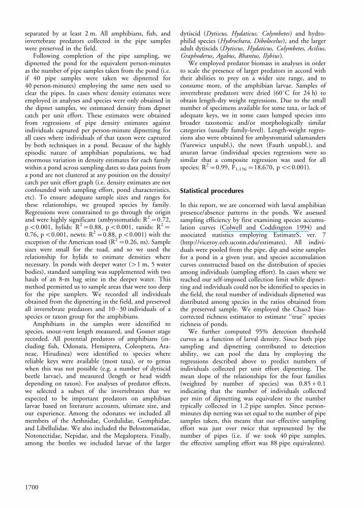
The ESGR wetlands (hereafter termed ponds)include a number of kettlehole ponds, swamps, marshesand Sphagnum bogs ranging up to 7 ha in area (Fig. 1).The terrestrial vegetation of the ESGR is dominated bygrasslands and hardwood forest (chiefly Quercus , Caryaand Acer as canopy dominants). There has been a steadysuccession of grasslands to forest following the clearingof much of the area by the 1850s and cessation ofagricultural activity in the first quarter of this century(from about 30% forest cover in 1940 to 80% in 1995,Skelly et al. 1999, Werner et al. unpubl.).

Seventeen amphibian species have been recordedbreeding on the ESGR, including representatives ofthree frog and three salamander families (Table 1).Two species were not collected in our survey;Plethodon cinereus is entirely terrestrial and Acriscrepitans went locally extinct on the ESGR in 1971due to a drought (Collins and Wilbur 1979). Thus,our sampling included 15 species. Of these 15, onewas not distinguished from Ambystoma laterale(A. tremblayi, which is a gynogenetic triploid hybridof the A. jeffersonianum complex with one set ofchromosomes from A. jeffersonianum and two from A.laterale , and is quite difficult to distinguish based onexternal characteristics, Uzzell 1964). Two other of thespecies, Rana palustris and Hemidactylum scutatum,were rare in our collections.

Fig. 1. Map of the E. S. George Reserve showing ponds thatwere sampled in black. Other wetland areas (few of whichsupport amphibian larvae) are shaded in the lighter color.

1698

Methods

Pond characteristics

Surface areas of the ESGR ponds were digitized fromaerial photographs (scale 1:3000) taken during thewinter of 1995 (when forest canopy did not obscureponds). In several of the marshes large central areas aredry and support terrestrial vegetation; hence theseregions were deleted from the pond area. The scaleemployed with the photographs was ground-truthedfrom measurement of artificial ponds and buildings onthe site. Pond areas ranged between 10 and 53 400 m2

(/x9se, 606892117), though the frequency distribu-tion was skewed to smaller ponds (73%B2500 m2).

Depth gauges were established in all ponds in the fallof 1998 and water levels were recorded at�1.5�2 weekintervals between late March and November. Weestimated pond hydroperiod as the average number ofdays that a pond held water divided by the number ofdays censused (ponds that held water in Novembertypically did not dry during the winter). If a pondcontained water on one census date and was dry on thenext, it was considered to have dried midway betweenthe dates. Prior to installing the depth gauges, werecorded status of the ponds when we sampled in Mayand July and noted if ponds were dry in the fall.Average pond hydroperiod (% of days the pond heldwater) ranged from 30 to 100% (/x across ponds 62.593.5%). Individual ponds, however, varied substantially

annually; in the extreme, ponds could range frompermanent in some years to holding water for only afew months in others.

Canopy cover was quantified using a sphericaldensiometer (Halverson et al. 2003). A minimum offive sites in each pond were chosen to take readings.The first site was the perceived center of the pond andthe four subsequent sites were determined by moving ineach of the four cardinal directions from the center sitetowards a position�2 m from the pond shore. In largerponds (n�26), more than 5 sites were needed toaccurately describe canopy cover. In these ponds,readings were made every 5 or 10 m depending onpond size along transects through the N-S and E-W axisof the pond. Four readings were taken at each samplingsite, one facing each cardinal direction. For all ponds,canopy cover was calculated by first averaging the fourreadings taken at each site (site mean), then averagingall site means for a pond. Canopy cover of the pondsranged fromB1 to 93% (/x�5995%).

The amphibian survey

The amphibian survey was conducted over sevenconsecutive years (1996�2002). We sampled larvalamphibians and their predators twice each year toestimate densities of both the spring- and summer-breeding amphibians. We sampled the third week inMay and July (with the exception of 1996 when wesampled 5/20�6/7 and 7/6�7/15; and 1997 when wesampled 6/9�6/24 and 7/28�8/2). Samples were takenby ‘‘pipe sampling’’, dipnetting and seining. The pipesampler was constructed of a 76 cm length of 36 cmdiameter aluminum pipe fitted with handles at the top;the pipe thus sampled 0.1 m2 of water column andsediments. The sample was taken by quietly approach-ing an area and quickly thrusting the pipe through thewater column and into the sediments to seal the samplearea. Nets (22�27 cm with a 1�2 mm mesh size)were employed to remove all animals from the sampledwater column and the first few centimeters of thesediments. Circular sweeps of the net were taken untilat least 10 consecutive sweeps were made withoutcapturing any animals (see Mullins et al. 2004 for anevaluation of these techniques).

Sampling effort varied with size of the pond: in smallponds (B750 m2) we took 20 pipe samples hapha-zardly distributed across representative microhabitats inthe ponds. In medium-sized ponds (�750 m2 butB1500 m2), we took 30�40 pipe samples acrossrepresentative microhabitats. In the largest ponds andmarshes (�1500 m2), we sampled along two transectsconsisting of 20 pipe samples each. Transect locationswere the same each year and traversed representativemicrohabitats in the pond. Pipe samples were always

Table 1. Amphibian species reported on the E. S. GeorgeReserve.

Family Species Common name

Bufonidae Bufo americanus American toadHylidae Acris crepitans cricket frog

Hyla versicolor gray tree frogPseudacris crucifer spring peeperP. triseriata chorus frog

Ranidae Rana catesbeiana bullfrogR. clamitans green frogR. pipiens leopard frogR. sylvatica wood frogR. palustris pickerel frog

Ambystomatidae Ambystoma laterale blue-spottedsalamander

A. maculatum spottedsalamander

A. tigrinum tigersalamander

A. tremblayi Tremblay’ssalamander

Plethodontidae Hemidactyliumscutatum

four-toedsalamander

Plethodon cinereus red-backedsalamander

Salamandridae Notophthalmusviridescens

eastern newt

1699

separated by at least 2 m. All amphibians, fish, andinvertebrate predators collected in the pipe sampleswere preserved in the field.

Following completion of the pipe sampling, wedipnetted the pond for the equivalent person-minutesas the number of pipe samples taken from the pond (i.e.if 40 pipe samples were taken we dipnetted for40 person-minutes) employing the same nets used toclear the pipes. In cases where density estimates wereemployed in analyses and species were only obtained inthe dipnet samples, we estimated density from dipnetcatch per unit effort. These estimates were obtainedfrom regressions of pipe density estimates againstindividuals captured per person-minute dipnetting forall cases where individuals of that taxon were capturedby both techniques in a pond. Because of the highlyepisodic nature of amphibian populations, we hadenormous variation in density estimates for each familywithin a pond across sampling dates so data points froma pond are not clustered at any position on the density/catch per unit effort graph (i.e. density estimates are notconfounded with sampling effort, pond characteristics,etc). To ensure adequate sample sizes and ranges forthese relationships, we grouped species by family.Regressions were constrained to go through the originand were highly significant (ambystomatids: R2�0.72,pB0.001, hylids: R2�0.88, pB0.001, ranids: R2�0.76, pB0.001, newts: R2�0.88, pB0.001) with theexception of the American toad (R2�0.26, ns). Samplesizes were small for the toad, and so we used therelationship for hylids to estimate densities wherenecessary. In ponds with deeper water (�1 m, 5 waterbodies), standard sampling was supplemented with twohauls of an 8-m bag seine in the deeper water. Thismethod permitted us to sample areas that were too deepfor the pipe samplers. We recorded all individualsobtained from the dipnetting in the field, and preservedall invertebrate predators and 10�30 individuals of aspecies or taxon group for the amphibians.

Amphibians in the samples were identified tospecies, snout-vent length measured, and Gosner stagerecorded. All potential predators of amphibians (in-cluding fish, Odonata, Hemiptera, Coleoptera, Ara-neae, Hirudinea) were identified to species wherereliable keys were available (most taxa), or to genuswhen this was not possible (e.g. a number of dytiscidbeetle larvae), and measured (length or head widthdepending on taxon). For analyses of predator effects,we selected a subset of the invertebrates that weexpected to be important predators on amphibianlarvae based on literature accounts, ultimate size, andour experience. Among the odonates we included allmembers of the Aeshnidae, Cordulidae, Gomphidae,and Libellulidae. We also included the Belostomatidae,Notonectidae, Nepidae, and the Megaloptera. Finally,among the beetles we included larvae of the larger

dytiscid (Dytiscus, Hydaticus, Colymbetes ) and hydro-philid species (Hydrochara, Dibolocelus ), and the largeradult dytiscids (Dytiscus, Hydaticus, Colymbetes, Acilius,Graphoderus, Agabus, Rhantus, Ilybius ).

We employed predator biomass in analyses in orderto scale the presence of larger predators in accord withtheir abilities to prey on a wider size range, and toconsume more, of the amphibian larvae. Samples ofinvertebrate predators were dried (608C for 24 h) toobtain length-dry weight regressions. Due to the smallnumber of specimens available for some taxa, or lack ofadequate keys, we in some cases lumped species intobroader taxonomic and/or morphologically similarcategories (usually family-level). Length-weight regres-sions also were obtained for ambystomatid salamanders(Yurewicz unpubl.), the newt (Fauth unpubl.), andanuran larvae (individual species regressions were sosimilar that a composite regression was used for allspecies; R2�0.99, F1,156�18,670, pBB0.001).

Statistical procedures

In this report, we are concerned with larval amphibianpresence/absence patterns in the ponds. We assessedsampling efficiency by first examining species accumu-lation curves (Colwell and Coddington 1994) andassociated statistics employing EstimateS, ver. 7(http://viceroy.eeb.uconn.edu/estimates). All indivi-duals were pooled from the pipe, dip and seine samplesfor a pond in a given year, and species accumulationcurves constructed based on the distribution of speciesamong individuals (sampling effort). In cases where wereached our self-imposed collection limit while dipnet-ting and individuals could not be identified to species inthe field, the total number of individuals dipnetted wasdistributed among species in the ratios obtained fromthe preserved sample. We employed the Chao2 bias-corrected richness estimator to estimate ‘‘true’’ speciesrichness of ponds.

We further computed 95% detection thresholdcurves as a function of larval density. Since both pipesampling and dipnetting contributed to detectionability, we can pool the data by employing theregressions described above to predict numbers ofindividuals collected per unit effort dipnetting. Themean slope of the relationships for the four families(weighted by number of species) was 0.85�0.1indicating that the number of individuals collectedper min of dipnetting was equivalent to the numbertypically collected in 1.2 pipe samples. Since person-minutes dip netting was set equal to the number of pipesamples taken, this means that our effective samplingeffort was just over twice that represented by thenumber of pipes (i.e. if we took 40 pipe samples,the effective sampling effort was 88 pipe equivalents).

1700

We could therefore use pipe equivalents to estimatedetection probabilities.

The basic patterns in species distributions weresummarized by an incidence matrix, which providesthe site by species presence/absence values. We con-structed a 14 species�36 pond (one pond never hadany species) incidence matrix and considered a speciespresent if it was encountered in that pond during any ofthe seven years. To test whether these incidencesdiffered from a null model of random placement ofspecies in ponds, we employed the approach of Leiboldand Mikkelson (2002). We first ordered rows andcolumns of the incidence matrix by ordination (reci-procal averaging), such that sites with the most similarspecies lists and species with the most similar distribu-tions were closest together. Employing the softwareprovided by Leibold and Mikkelson (2002), we thentested this matrix to determine if there was a strongdominant axis of variation, and if so, whether thematrix was characterized by species turnover or nestedsubsets, and whether there was strong clumping ofspecies boundaries.

Model formulationThe incidence matrix presented patterns in the associa-tion of individual species with different environmentalcharacteristics and each other based on cumulativepresences. We also were interested in the patterns ofamphibian species richness in ponds, and identifyingthe local factors that influenced species richness. It isnot clear what time scale actually best captures regula-tion of community structure in this system, but becauseof incidental presences and effects of extreme years (insome case resulting in the loss of fish) cumulativerichness could be problematic. Therefore, we askedwhat the relation was between long-term averageenvironmental and biotic conditions and the long-term average species richness of a pond. We employed amodel selection approach to identify the most appro-priate statistical model for predicting amphibian speciesrichness from local factors. Formulating models fortotal amphibian species richness of ponds with bioticfactors is difficult as these communities are composed ofspecies occupying two trophic levels; i.e. carnivorouscaudates (salamanders) and herbivorous/detritivorousanuran larvae. Consequently, we formulated modelsseparately for these two orders. The local abioticvariables included in the models were pond hydroper-iod, area and forest canopy cover. Local biotic variablesincluded biomasses of anuran larvae, caudate larvae andinvertebrate predators (all per m2). We employed Maybiomasses in these analyses reasoning that this biomassdensity was the most likely to influence both the springbreeders and the early larval phase of the summerbreeders. Most species in this community were spring

breeders and even summer breeders, when small,overlapped to some extent with these species. Moreover,the average biomass of anuran larvae across all pondswas 2.4-fold higher in May than in July (t-test, t�2.7,DF�60, p�0.01), and the ambystomatid salamandersall breed in the spring.

All three of the abiotic variables are known to beassociated with species richness of amphibian commu-nities and there are biologically plausible mechanismsby which these factors could influence both anurans andcaudates (Skelly et al. 1999, Van Buskirk 2005). Bioticfactors have a somewhat different interpretation for thetwo taxa. For anurans, biomass represents potentialcompetitive effects, and caudate and invertebratebiomass represent potential predatory effects (thesewere maintained as separate variables because ofpotential differences in their modes of predation andthe fact that caudate biomass can often swamp that ofinvertebrate predators in many of the ponds). Forcaudates, invertebrate biomass represents potentialpredators, caudate biomass potential competitors (thelatter variable, however, could include effects generatedboth through competition and intraguild predation),and anuran biomass potential prey.

The global models for both taxa therefore includedall six of these local abiotic and biotic variables. Wethen formulated two further models that postulatedonly the effects of local abiotic or biotic effects wereimportant, and therefore each of these models includedthe three relevant variables. The models were formu-lated for ponds without fish (or years without fish). Wehad a relatively small number of ponds with fish for allseven years, and the impact of fish renders manyrelationships on environmental variables quadraticthat are otherwise linear.

We employed AICc, a bias-corrected version ofAkaike’s information criterion, to rank models accord-ing to the strength of support from the data (Burnhamand Anderson 2002). The best model is that with thelowest AICc value, and we employed Akaike weights toassess the likelihood of alternative models. Akaikeweights also were used to estimate parameter valuesand their variances employing a model averagingapproach (Burnham and Anderson 2002). Modelaveraged estimates and SE’s were calculated and 95%confidence intervals employed to assess the magnitudeof the effect. We concluded that there was an effect ifthe confidence interval excluded 0.

The Akaike model selection procedure seeks thesingle best supported predictive model, but thisapproach does not identify those variables most likelyto influence variation in the response variable (speciesrichness in our case). Abiotic and biotic predictorvariables were often significantly intercorrelated. Suchmulticollinearity makes it difficult to identify variablesthat have independent effects on the response variable.

1701

In order to identify important potential causal vari-ables having independent effects on species richness weemployed hierarchical partitioning (Mac Nally 2002,Quinn and Keough 2006). Hierarchical partitioningemploys goodness of fit measures (R2 in a multipleregression setting) and averages the incremental im-provement in fit by the addition of a given variable toall of the possible models (2k models for k predictorvariables) with that variable compared to the equiva-lent model without that variable. Using this methodone can partition explanatory power for each predictorvariable into independent effects and those due tojoint effects with other variables (i.e. those that cannotbe unambiguously associated with the variable inquestion). For both anurans and caudates we includedall six abiotic and biotic variables listed above in theseanalyses. We further employed a method randomizingthe data suggested by Mac Nally (2002) to statisticallyevaluate which predictor variables should be retained(analyses conducted in R, R Development Core Team2006). For some analyses we also employed principalcomponents analyses to extract orthogonal measures ofsite heterogeneity. In all cases the first principalcomponent was employed and accounted for a largefraction of the variation (and was the only compo-nent retained by the broken-stick criterion, Jackson1993).

Results

Sampling effectiveness

While detection errors are an inevitable part ofsurveying occupancy, our analyses suggest that we hadexcellent power to detect species overall. Estimators ofspecies richness from sampling effort typically convergeon the observed species number when all species arerepresented by two or more individuals in the collection(Colwell and Coddington 1994). This was the case in64% of our 219 pond � year combinations. Cases withsingletons (species represented by a single individual inthe sample) that are adequately sampled versus inade-quately sampled can look substantially the same(Colwell and Coddington 1994), so in these cases weemployed the Chao2 richness estimator in EstimateS toestimate the species richness of the pond that year. Inonly 5% of the total number of pond-year combina-tions did the theoretically estimated number of speciesexceed the actual number sampled by�0.5. Further,there was no relation (R2�4�10�6) between thefraction of records in a pond that were singletons andthe sampling effort in that pond (measured as pondarea/no. of pipe samples taken, which varied over a 212-fold range because we were unable to sample very largemarshes with the same effort as small ponds). Finally,

the detection threshold analysis indicated that if larvaewere assumed (as a first approximation) to be binomi-ally or Poisson distributed, our 95% detection thresh-old for a species occurred at densities on the order of1 larva per 3.3 m2 in the larger ponds.

Community coherence

There were consistent patterns in species distributionsacross the ESGR ponds; the incidence matrix exhibitedstrong coherence with species associations differingsignificantly from random placement of species(Fig. 2). The row ordination of the matrix (Fig. 2)describes the dominant axis of variation in speciescomposition among ponds and these ordination scoreswere positively correlated with pond area and hydro-period, and negatively correlated with canopy cover(pB0.001 for all regressions).

Species ranges across the dominant axis exhibitedsignificant turnover (i.e. species tended to replace eachother from site to site, pB0.05). Further, rangeboundaries were significantly clumped (Morisita’sindex�2.50, pB0.001). Species replacements oc-curred primarily at the extremes of the major axis ofvariation (Fig. 2), with species boundaries stronglyclumped near these extremes. This strong clumping wasassociated with pond canopy cover (below) at the upperextreme of the matrix and with predatory fish andpermanent water at the lower extreme.

Communities also were significantly nested (i.e.communities of species-poor ponds tended to be subsetsof those of species-rich ponds (pB0.01). There was astrong tendency for communities in ponds with highcanopy cover, small area and short hydroperiod to benested subsets of those with the contrasting character-istics (Fig. 2). The incidence matrix was constituted ofcumulative species presences and included cases of aspecies found only incidentally in a pond. Identicalresults for all tests were obtained if we constructed theincidence matrix with a more stringent species presencecriterion (i.e. requiring a species to be present in thepond at least two of the seven years).

The matrix ordination places species closest to-gether that have the most similar distributions and thisordering exhibited strong clustering by family. Theranids exhibited a tendency to be associated with morepermanent water and fish. The glaring exception wasRana sylvatica , which was separated from the otherranids because it was found in shorter hydroperiodand closed-canopy ponds. The ranids were followed bythe newt and then a cluster of all three hylids. Theseare smaller species with shorter larval periods thatcan inhabit more temporary environments, thoughstill largely open-canopy environments. The nextcluster includes the ambystomatid salamanders and

1702

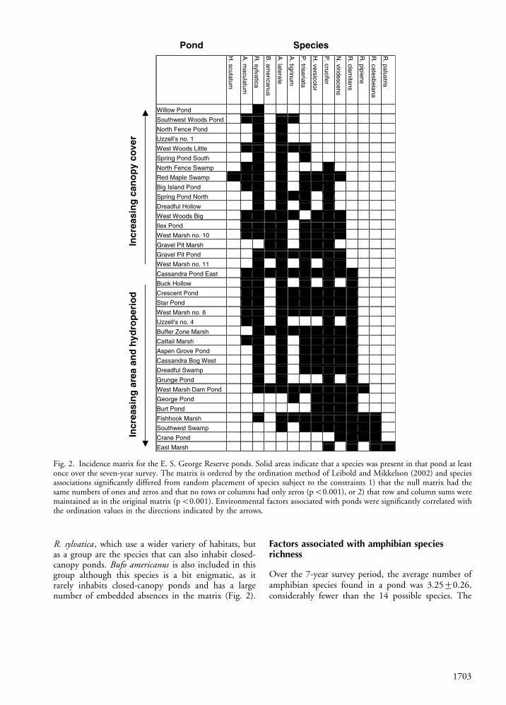
R. sylvatica , which use a wider variety of habitats, butas a group are the species that can also inhabit closed-canopy ponds. Bufo americanus is also included in thisgroup although this species is a bit enigmatic, as itrarely inhabits closed-canopy ponds and has a largenumber of embedded absences in the matrix (Fig. 2).

Factors associated with amphibian speciesrichness

Over the 7-year survey period, the average number ofamphibian species found in a pond was 3.2590.26,considerably fewer than the 14 possible species. The

Fig. 2. Incidence matrix for the E. S. George Reserve ponds. Solid areas indicate that a species was present in that pond at leastonce over the seven-year survey. The matrix is ordered by the ordination method of Leibold and Mikkelson (2002) and speciesassociations significantly differed from random placement of species subject to the constraints 1) that the null matrix had thesame numbers of ones and zeros and that no rows or columns had only zeros (pB0.001), or 2) that row and column sums weremaintained as in the original matrix (pB0.001). Environmental factors associated with ponds were significantly correlated withthe ordination values in the directions indicated by the arrows.

1703

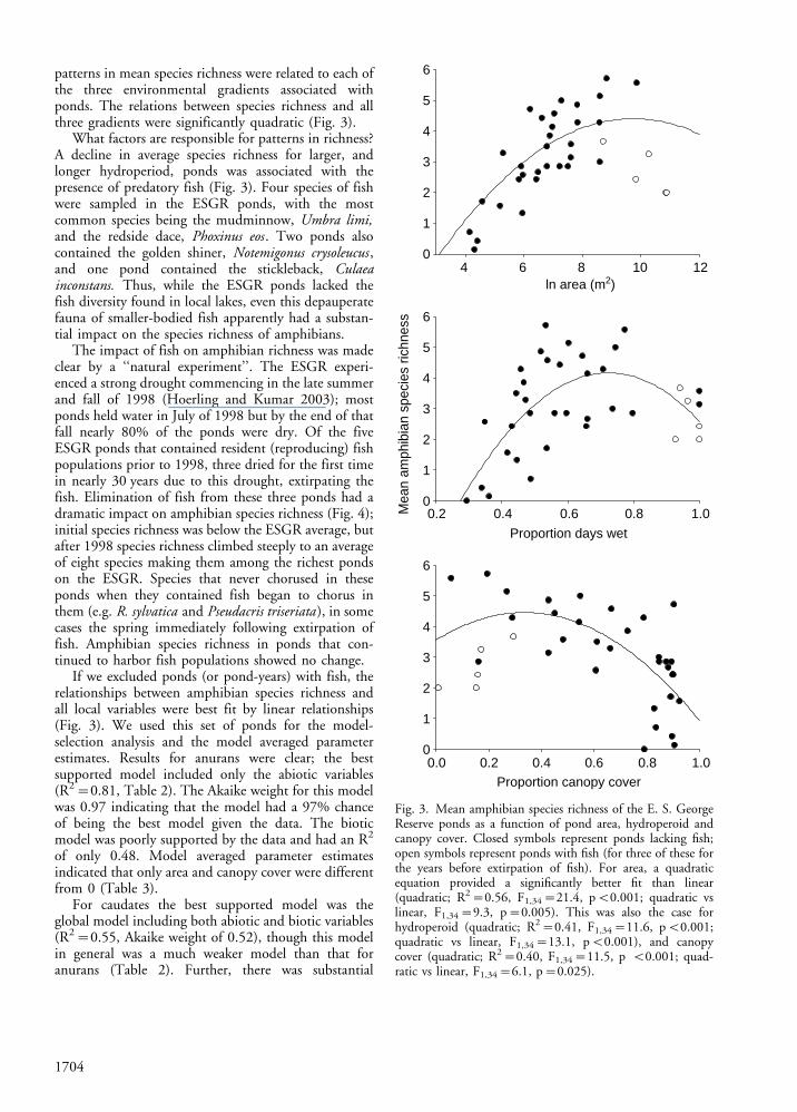
patterns in mean species richness were related to each ofthe three environmental gradients associated withponds. The relations between species richness and allthree gradients were significantly quadratic (Fig. 3).

What factors are responsible for patterns in richness?A decline in average species richness for larger, andlonger hydroperiod, ponds was associated with thepresence of predatory fish (Fig. 3). Four species of fishwere sampled in the ESGR ponds, with the mostcommon species being the mudminnow, Umbra limi,and the redside dace, Phoxinus eos . Two ponds alsocontained the golden shiner, Notemigonus crysoleucus ,and one pond contained the stickleback, Culaeainconstans. Thus, while the ESGR ponds lacked thefish diversity found in local lakes, even this depauperatefauna of smaller-bodied fish apparently had a substan-tial impact on the species richness of amphibians.

The impact of fish on amphibian richness was madeclear by a ‘‘natural experiment’’. The ESGR experi-enced a strong drought commencing in the late summerand fall of 1998 (Hoerling and Kumar 2003); mostponds held water in July of 1998 but by the end of thatfall nearly 80% of the ponds were dry. Of the fiveESGR ponds that contained resident (reproducing) fishpopulations prior to 1998, three dried for the first timein nearly 30 years due to this drought, extirpating thefish. Elimination of fish from these three ponds had adramatic impact on amphibian species richness (Fig. 4);initial species richness was below the ESGR average, butafter 1998 species richness climbed steeply to an averageof eight species making them among the richest pondson the ESGR. Species that never chorused in theseponds when they contained fish began to chorus inthem (e.g. R. sylvatica and Pseudacris triseriata ), in somecases the spring immediately following extirpation offish. Amphibian species richness in ponds that con-tinued to harbor fish populations showed no change.

If we excluded ponds (or pond-years) with fish, therelationships between amphibian species richness andall local variables were best fit by linear relationships(Fig. 3). We used this set of ponds for the model-selection analysis and the model averaged parameterestimates. Results for anurans were clear; the bestsupported model included only the abiotic variables(R2�0.81, Table 2). The Akaike weight for this modelwas 0.97 indicating that the model had a 97% chanceof being the best model given the data. The bioticmodel was poorly supported by the data and had an R2

of only 0.48. Model averaged parameter estimatesindicated that only area and canopy cover were differentfrom 0 (Table 3).

For caudates the best supported model was theglobal model including both abiotic and biotic variables(R2�0.55, Akaike weight of 0.52), though this modelin general was a much weaker model than that foranurans (Table 2). Further, there was substantial

ln area (m2)4 6 8 10 12

0

1

2

3

4

5

6

Proportion days wet

0.2 0.4 0.6 0.8 1.0

0.20.0 0.4 0.6 0.8 1.0

Mea

n am

phib

ian

spec

ies

richn

ess

0

1

2

3

4

5

6

Proportion canopy cover

0

1

2

3

4

5

6

Fig. 3. Mean amphibian species richness of the E. S. GeorgeReserve ponds as a function of pond area, hydroperoid andcanopy cover. Closed symbols represent ponds lacking fish;open symbols represent ponds with fish (for three of these forthe years before extirpation of fish). For area, a quadraticequation provided a significantly better fit than linear(quadratic; R2�0.56, F1,34�21.4, pB0.001; quadratic vslinear, F1,34�9.3, p�0.005). This was also the case forhydroperoid (quadratic; R2�0.41, F1,34�11.6, pB0.001;quadratic vs linear, F1,34�13.1, pB0.001), and canopycover (quadratic; R2�0.40, F1,34�11.5, p B0.001; quad-ratic vs linear, F1,34�6.1, p�0.025).

1704

support for all models indicating a relatively largeamount of uncertainty regarding the best model (Table2). Model averaged parameter estimates and confidenceintervals indicated only area was significantly differentfrom 0, though caudate and invertebrate predatorbiomass were nearly significant (Table 3).

These analyses therefore indicated strong support fora statistical model of abiotic factors for anurans andinclusion of these variables in the model for caudates.However, it is not clear from these analyses whether all

of these variables are independently contributing tovariation in species richness, or if variables are includedin the model because they contribute to the overall bestfit due to correlations with causal variables. Further, it isnot clear if all independently contributing variables areincluded in the selected models. The three environ-mental variables were moderately collinear (varianceinflation factors ranging from 2.1�4.5); smaller pondsexhibited more extensive forest canopy cover, and,in general, possessed shorter hydroperiods. Thus,hydroperiod was positively (r�0.74, F1,35�41.3,pB0.001), and canopy cover negatively (r�0.78,F1,35�52.6, pB0.001), correlated with pond area,and canopy cover negatively correlated with hydroper-iod (r�0.52, F1,35�13.1, pB0.001). Caudate andanuran biomass were not significantly correlated withany of the other variables. However, invertebratepredator biomass was significantly positively correlatedwith area (r�0.66, F1,31�24.1, pB0.001) andhydroperiod (r�0.49, F1,31�9.8, p�0.004) andsignificantly negatively correlated with canopy cover(r�0.63, F1,31�20.8, pB0.001).

To identify the extent to which these variables wereindependently related to species richness, we employedhierarchical partitioning. The results of the analyseslargely reinforced those of the model selection exercisewith specific exceptions. For anurans, area and canopycover alone accounted for 71% of the independenteffects of all variables (Table 4). This is consistent withthe model selection analysis, which indicated greatestsupport for the abiotic model and significant model

Table 2. Model selection results for predicting average species richness of anurans and caudates in ponds.

Number of parameters n Residual SS AICc Di Wi

Anuran modelAbiotic variables 5 33 11.3 �23.1 0.0 0.97Biotic variables 5 33 30.1 9.2 32.3 0.00Global model 8 33 10.3 �16.4 6.7 0.03R2 of the best model�0.81

Caudate modelAbiotic variables 5 33 8.5 �32.6 1.3 0.27Biotic variables 5 33 8.6 �32.2 1.8 0.22Global model 5 33 6.1 �34.0 0.0 0.52R2 of the best model�0.55

Table 3. Model-averaged parameter values for anurans and caudates. Bold values are those where 95% confidence intervalsexcluded 0.

Parameter Area Canopy cover Hydroperiod Invertebrate predators Caudate biomass Anuran biomass

Anuransestimate 0.40 �2.14 0.36 0.005 0.0007 0.00002SE 0.13 0.62 0.77 0.008 0.0008 0.00002

Caudatesestimate 0.22 0.45 0.72 0.01 0.001 0.00002SE 0.11 0.53 0.64 0.007 0.0007 0.00002

Year

1996 1997 1998 1999 2000 2001 2002

Mea

n am

phib

ian

spec

ies

richn

ess

1

2

3

4

5

6

7

8

9

Fig. 4. Mean amphibian species richness of E. S. GeorgeReserve ponds across years. Closed symbols represent pondsthat lost fish in the fall of 1998 or during 1999 (West MarshDam Pond, Fishhook Marsh and Southwest Swamp); opensymbols are all other ponds.

1705

averaged parameter estimates for area and canopy cover.Hierarchical partitioning, however, also indicated thatinvertebrate predator biomass accounted for 17% of theindependent effects (Table 4). Area, canopy cover andinvertebrate predator biomass were significant by therandomization technique.

For caudates, the model selection procedure indi-cated that the global model was the best supportedmodel. Congruent with this result, hierarchical parti-tioning indicated that four of the predictor variablescontributed between 9 and 16% of the independenteffects, and three of these were significant by therandomization technique (area, hydroperiod and in-vertebrate predator biomass, Table 4).

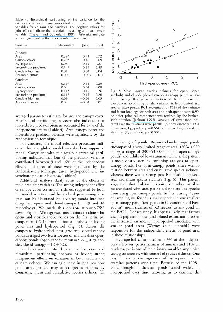
Additional analyses clarify some of the effects ofthese predictor variables. The strong independent effectof canopy cover on anuran richness suggested by boththe model selection and hierarchical partitioning ana-lyses can be illustrated by dividing ponds into twocategories, open- and closed-canopy (n�19 and 14respectively). We made this division at�or575%cover (Fig. 3). We regressed mean anuran richness foropen- and closed-canopy ponds on the first principalcomponent (PC1) from a factor analysis includingpond area and hydroperiod (Fig. 5). Across thecomposite hydroperiod�area gradient, closed-canopyponds averaged two fewer species of anurans than open-canopy ponds (open-canopy mean�3.2790.25 spe-cies, closed-canopy�1.290.2).

Pond area was identified by the model selection andhierarchical partitioning analyses as having strongindependent effects on variation in both anuran andcaudate richness. We can gain some insight into howpond area, per se, may affect species richness bycomparing mean and cumulative species richness (all

amphibians) of ponds. Because closed-canopy pondsencompassed a very limited range of areas (80%B900m2 vs a range of 200�53 000 m2 for open-canopyponds) and exhibited lower anuran richness, the patternis most clearly seen by confining analyses to open-canopy ponds. For open-canopy ponds, there was norelation between area and cumulative species richness,whereas there was a strong positive relation betweenarea and mean species richness (Fig. 6). This patternsuggested that habitat diversity or other attribu-tes associated with area per se did not exclude speciesfrom using open-canopy ponds. In fact, during 7 yearsof sampling we found as many species in our smallestopen-canopy pond (ten species in Cassandra Pond East,200 m2, mean richness of 3.3 species) as any pond onthe ESGR. Consequently, it appears likely that factorssuch as population size (and related extinction rates) orthe increased variance in hydroperiod associated withsmaller pond areas (Werner et al. unpubl.) wereresponsible for the independent effects of pond areain these relationships.

Hydroperiod contributed only 9% of the indepen-dent effect on species richness of anurans and 21% oncaudates, yet is one of the primary variables amphibianecologists associate with control of species richness. Oneway to isolate the signature of hydroperiod is toexamine patterns over time. Because of the 1998�2002 drought, individual ponds varied widely inhydroperiod over time, allowing us to examine the

Table 4. Hierarchical partitioning of the variance for the64 models in each case associated with the 6 predictorvariables for anurans and caudates. The negative values forjoint effects indicate that a variable is acting as a suppressorvariable (Chevan and Sutherland 1991). Asterisks indicatevalues significant by the randomization procedure.

Variable Independent Joint Total

AnuransArea 0.29* 0.43 0.72Canopy cover 0.29* 0.40 0.69Hydroperiod 0.08 0.19 0.27Invertebrate predators 0.14* 0.31 0.45Caudate biomass 0.01 0.03 0.04Anuran biomass 0.006 0.005 0.011

CaudatesArea 0.16* 0.13 0.29Canopy cover 0.04 0.05 0.09Hydroperiod 0.11* 0.15 0.26Invertebrate predators 0.11* 0.15 0.26Caudate biomass 0.09 �0.04 0.05Anuran biomass 0.03 �0.02 0.01

Hydroperiod-area PC1

-2 -1 0 1 2 3

Mea

n an

uran

spe

cies

ric

hnes

s

0

1

2

3

4

5

6

7

Fig. 5. Mean anuran species richness for open- (opensymbols) and closed- (closed symbols) canopy ponds on theE. S. George Reserve as a function of the first principalcomponent accounting for the variation in hydroperiod andarea of these ponds. PC1 accounted for 81% of the varianceand factor loadings for both area and hydroperiod were 0.90,no other principal component was retained by the broken-stick criterion (Jackson 1993). Analysis of covariance indi-cated that the relations were parallel (canopy category�PC1interaction, F1,29�0.2, p�0.66), but differed significantly inelevation (F1,29�28.6, pB0.001).

1706

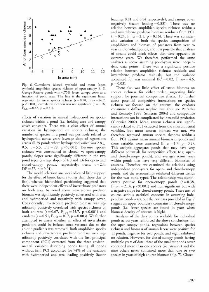
effects of variation in annual hydroperiod on speciesrichness within a pond (i.e. holding area and canopycover constant). There was a clear effect of annualvariation in hydroperiod on species richness; thenumber of species in a pond was positively related tohydroperiod across years (average slope of regressionsacross all 29 ponds where hydroperiod varied was 2.890.5, t�5.5, DF�28, pB0.001). Because speciesrichness was constrained in closed- vs open-canopyponds, slopes were significantly different in the twopond types (average slopes of 4.0 and 1.6 for open- andclosed-canopy ponds, respectively; t-test, t�2.4,DF�27, p�0.01).

The model selection analyses indicated little supportfor the effect of biotic factors (other than those due tofish), whereas hierarchical partitioning suggested thatthere were independent effects of invertebrate predatorson both taxa. As noted above, invertebrate predatorbiomass was significantly positively correlated with areaand hydroperiod and negatively with canopy cover.Consequently, invertebrate predator biomass was sig-nificantly positively correlated with species richness ofboth anurans (r�0.67, F1,31�25.7, pB0.001) andcaudates (r�0.51, F1,31�10.7, p�0.003). We furtherattempted to assess whether an effect of invertebratepredators could be isolated once variance due to theabiotic gradients was removed. Both amphibian speciesrichness and invertebrate predator biomass were sig-nificantly positively correlated with the first principalcomponent (PC1) extracted from the three environ-mental variables describing ponds (using all pondswithout fish; PC1 accounted for 74% of the variationwith hydroperiod and area loading positively (factor

loadings 0.81 and 0.94 respectively), and canopy covernegatively (factor loading�0.83)). There was norelation between amphibian species richness residualsand invertebrate predator biomass residuals from PC1(r�0.24, F1,,33�2.1, p�0.16). There was consider-able variation in both the species composition ofamphibians and biomass of predators from year toyear in individual ponds, and it is possible that analysesof means could mask effects that were apparent inextreme years. We therefore performed the sameanalyses as above assuming pond-years were indepen-dent data points. There was a significant positiverelation between amphibian richness residuals andinvertebrate predator residuals, but the varianceaccounted for was minimal (R2�0.02, F1,207�4.6,p�0.03).

There also was little effect of taxon biomass onspecies richness for either order, suggesting littlesupport for potential competitive effects. To furtherassess potential competitive interactions on speciesrichness we focused on the anurans; the caudatesconstitute a different trophic level (but see Petrankaand Kennedy 1999, Schiesari 2004) and competitiveinteractions can be complicated by intraguild predation(Yurewicz 2002). Mean anuran richness was signifi-cantly related to PC1 extracted from the environmentalvariables, but mean anuran biomass was not. Wetherefore regressed anuran species richness residualsfrom PC1 against mean anuran biomass in ponds andthese variables were unrelated (F1,30�1.7, p�0.2).This analysis aggregates ponds that may have verydifferent potentials for competitive effects (e.g. open-and closed-canopy ponds), and averages across yearswithin ponds that have very different biomasses ofanurans. Therefore, we examined the relations usingindependent pond-years for open- and closed-canopyponds, and the relationships exhibited different trendsfor the two pond types. The relationship was signifi-cantly positive for open-canopy ponds (r�0.38,F1,131�21.4, pB0.001) and non significant but witha negative slope for closed-canopy ponds. There are, ofcourse, serious statistical concerns in assuming inde-pendent pond-years, but the raw data provided in Fig. 7suggest an upper boundary constraint in closed-canopyponds (i.e. fewer species are found in years whenbiomass density of anurans is high).

Analyses of the data points available for individualponds across years reinforced the above conclusions; forthe open-canopy ponds, regressions between speciesrichness and biomass of anuran larvae were positive for11 ponds, negative for two ponds, and eight exhibitedno relation. However, for closed-canopy ponds havingmultiple years of data, three of the smallest ponds nevercontained more than one species (R. sylvatica ) and thenine others never contained more than one or twospecies in years of high anuran biomass (Fig. 7). Closed-

ln area (m2)

5 6 7 8 9 10 11 12

Am

phib

ian

spec

ies

richn

ess

0

2

4

6

8

10

12

Fig. 6. Cumulative (closed symbols) and mean (opensymbols) amphibian species richness of open-canopy E. S.George Reserve ponds withB75% forest canopy cover as afunction of pond area. The line is the significant linearregression for mean species richness (r�0.78, F1,17�26.2,pB0.001), cumulative richness was not significant (r�0.16,F1,17�0.45, p�0.51).

1707

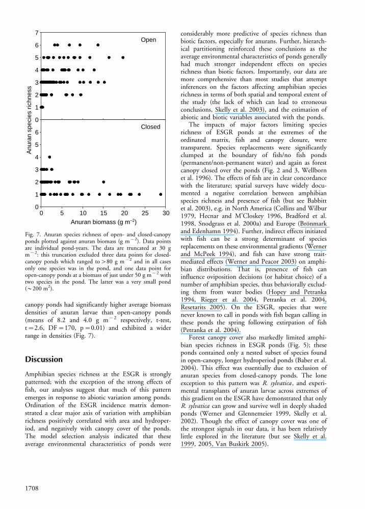
canopy ponds had significantly higher average biomassdensities of anuran larvae than open-canopy ponds(means of 8.2 and 4.0 g m�2 respectively, t-test,t�2.6, DF�170, p�0.01) and exhibited a widerrange in densities (Fig. 7).

Discussion

Amphibian species richness at the ESGR is stronglypatterned; with the exception of the strong effects offish, our analyses suggest that much of this patternemerges in response to abiotic variation among ponds.Ordination of the ESGR incidence matrix demon-strated a clear major axis of variation with amphibianrichness positively correlated with area and hydroper-iod, and negatively with canopy cover of the ponds.The model selection analysis indicated that theseaverage environmental characteristics of ponds were

considerably more predictive of species richness thanbiotic factors, especially for anurans. Further, hierarch-ical partitioning reinforced these conclusions as theaverage environmental characteristics of ponds generallyhad much stronger independent effects on speciesrichness than biotic factors. Importantly, our data aremore comprehensive than most studies that attemptinferences on the factors affecting amphibian speciesrichness in terms of both spatial and temporal extent ofthe study (the lack of which can lead to erroneousconclusions, Skelly et al. 2003), and the estimation ofabiotic and biotic variables associated with the ponds.

The impacts of major factors limiting speciesrichness of ESGR ponds at the extremes of theordinated matrix, fish and canopy closure, weretransparent. Species replacements were significantlyclumped at the boundary of fish/no fish ponds(permanent/non-permanent water) and again as forestcanopy closed over the ponds (Fig. 2 and 3, Wellbornet al. 1996). The effects of fish are in clear concordancewith the literature; spatial surveys have widely docu-mented a negative correlation between amphibianspecies richness and presence of fish (but see Babbittet al. 2003), e.g. in North America (Collins and Wilbur1979, Hecnar and M’Closkey 1996, Bradford et al.1998, Snodgrass et al. 2000a) and Europe (Bronmarkand Edenhamn 1994). Further, indirect effects initiatedwith fish can be a strong determinant of speciesreplacements on these environmental gradients (Wernerand McPeek 1994), and fish can have strong trait-mediated effects (Werner and Peacor 2003) on amphi-bian distributions. That is, presence of fish caninfluence oviposition decisions (or habitat choice) of anumber of amphibian species, thus behaviorally exclud-ing them from water bodies (Hopey and Petranka1994, Rieger et al. 2004, Petranka et al. 2004,Resetarits 2005). On the ESGR, species that werenever known to call in ponds with fish began calling inthese ponds the spring following extirpation of fish(Petranka et al. 2004).

Forest canopy cover also markedly limited amphi-bian species richness in ESGR ponds (Fig. 5); theseponds contained only a nested subset of species foundin open-canopy, longer hydroperiod ponds (Baber et al.2004). This effect was essentially due to exclusion ofanuran species from closed-canopy ponds. The loneexception to this pattern was R. sylvatica , and experi-mental transplants of anuran larvae across extremes ofthis gradient on the ESGR have demonstrated that onlyR. sylvatica can grow and survive well in deeply shadedponds (Werner and Glennemeier 1999, Skelly et al.2002). Though the effect of canopy cover was one ofthe strongest signals in our data, it has been relativelylittle explored in the literature (but see Skelly et al.1999, 2005, Van Buskirk 2005).

Anu

ran

spec

ies

richn

ess

Anuran biomass (g m–2)0 5 10 15 20 25 30

0

1

2

3

4

5

6

0

1

2

3

4

5

6

7Open

Closed

Fig. 7. Anuran species richness of open- and closed-canopyponds plotted against anuran biomass (g m�2). Data pointsare individual pond-years. The data are truncated at 30 gm�2: this truncation excluded three data points for closed-canopy ponds which ranged to�80 g m�2 and in all casesonly one species was in the pond, and one data point foropen-canopy ponds at a biomass of just under 50 g m�2 withtwo species in the pond. The latter was a very small pond(�200 m2).

1708

There are clear mechanisms that may account for theeffect of forest canopy cover; canopy cover dramaticallyaffects resource availability and quality as well as abioticconditions in a pond (Werner and Glennemeier 1999,Skelly et al. 2002, Halverson et al. 2003, Schiesari2004). C:N ratios of both tadpole gut contents andnatural foods indicate that resources are of lowernutritional quality in closed-canopy ponds, and experi-mental studies suggest that (power-efficiency) tradeoffsoften seen in species replacing each other on produc-tivity gradients are responsible for differences in speciesperformance (Schiesari 2004, Schiesari et al. 2006).Further, the influence of canopy cover appears to bestrong enough in some cases to lead to local adaptationin species (Relyea 2002, Skelly 2004). The effect ofcanopy cover is likely restricted to the anurans due inpart to the effects of reduced light levels on theirresources. The caudates, which in contrast are carnivor-ous, appear to be relatively unaffected by canopy cover(i.e. largely subsisting on a detritus-based food chain).Given strong effects of forest cover on both the larvaland terrestrial phases of a number of amphibian species(Hecnar and M’Closkey 1998, Skelly et al. 1999, 2005,Houlahan and Findlay 2003, Schiesari 2004) thewidespread succession of forested landscapes (especiallyover much of eastern North America) would beexpected to have wide-ranging effects on amphibiancommunities.

Pond area had substantial independent effects onspecies richness of both taxa. Reports in the literaturegenerally indicate little evidence of a relation betweenamphibian species richness and pond area (Hecnar andM’Closkey 1996, Snodgrass et al. 2000b, but seeHoulahan and Findlay 2003), but the smallest pondsin most of these studies are considerably larger thanours. As noted earlier the contrast in mean andcumulative species richness in these ponds (Fig. 6)suggests that effects of small population sizes andenhanced variation in hydroperiod, were the importantfactors determining the lower mean richness in smallerponds. In fact, there is a strong negative relationbetween extinction rate and pond area on the ESGR,and the variance in hydroperiod increases nonlinearlywith decline in mean hydroperiod (Werner et al. 2007).Therefore, because of frequent extinctions in theseponds, spatial context and connectivity between pondsshould strongly influence the effect of area, e.g. ifisolated from other ponds, pond size could becomemore important than indicated here.

Perhaps the most widely cited factor influencingamphibian species richness is pond hydroperiod (Skelly2001, for recent survey studies see Snodgrass et al.2000a, 2000b, Babbitt et al. 2003). The expectationthat amphibian species richness should exhibit aunimodal curve peaking at intermediate hydroperiodswas articulated by Heyer et al. (1975) and Wilbur

(1984), and generalized to additional taxa incorporatingthe role of life history tradeoffs and predator transitionson the hydroperiod gradient by Wellborn et al. (1996).Hydroperiod exhibited the weakest independent signalof the environmental gradients in our data, but thetemporal extent of our survey and the increasingdisparity between mean and cumulative richness withdecline in pond area (Fig. 6) enabled us to show a cleareffect of hydroperiod on species richness within a pond.Years of shorter hydroperiods typically excluded the latespring and summer breeders from ponds (Semlitschet al. 1996). The significant nesting of species in theESGR amphibian community (Fig. 2) also suggests thatthe disturbance (hydroperiod) gradient is importantbecause of developmental constraints (larval period,Urban 2004). The constraints of hydroperiod appear tobe largely temporary as species requiring longer hydro-periods quickly take advantage of local climatic varia-tion leading to extended hydroperiods in specific ponds.Again, this factor should strongly interact with spatialcontext or connectivity of the ponds, as extinctions dueto climate variation affecting hydroperiod requirerecolonization from other ponds, and therefore meanrichness of a pond will depend on how often this occurs(Werner et al. 2007).

Thus, effects of abiotic factors on amphibian speciesrichness exhibited in our data appear strong andsupported by plausible mechanisms. Evidence for theeffects of biotic factors on species richness of ponds wasless compelling. With the exception of fish, evidencefrom the field of the impact of predators on amphibianspecies richness is scant or mixed (Skelly 2001, 2002,but see Smith and Van Buskirk 1995, Fauth 1999).Hierarchical partitioning indicated independent corre-lations between invertebrate predators and speciesrichness of both anurans and caudates. Since theserelationships were strongly positive, potential mechan-isms responsible include keystone predator effects or thefact that invertebrate predators were correlated withadditional environmental factors that were unmeasured.Van Buskirk (2005) in assessing occurrences of in-dividual species in a European community also foundthat in three of the four cases where model averagedparameter estimates were significant, correlations withpredators were positive. We do not see correlationsconsistent with strong competitive effects for theanurans in the larger open-canopy (and predator-rich,Schneider and Frost 1996) ponds, suggesting that akeystone predator effect is less likely. The strongbehavioral and morphological responses of manyamphibian larvae to invertebrate predators indicatethat these predators have been a significant selectiveforce on larval traits (Relyea 2001, Van Buskirkand Arioli 2005), and may have density effects orpotentially limit certain species (Werner and McPeek1994, Smith and Van Buskirk 1995, Babbitt et al.

1709

2003). Experimental work will be required to deter-mine if these correlations actually represent effects ofpredators. Unfortunately, we were unable to assess theimpact of other vertebrate predators that may affectthese amphibian communities, e.g. turtles, snakes andraccoons.

Interspecific competition among amphibian larvaehas received a great deal of attention, and can havestrong effects under controlled experimental conditions(Wilbur 1997, Skelly 2002). However, evidence fromthe field is scarcer, especially for effects on speciesrichness. There was no signal in our data thatcompetitive effects limited species richness in open-canopy ponds. Species richness relationships werepositive with anuran biomass suggesting that theaddition of new species simply added biomass withoutaffecting presence of other species, and/or that goodyears for many species were coincident. Similarly, VanBuskirk (2005) also found that the occurrences of allspecies in a European community were positivelycorrelated with densities of other species, indicatingthat if competition was important it was overwhelmedby the positive effects of site quality. In many regardsthis pattern might be expected in larger open-canopyponds which are much less likely to be saturated withlarvae from the surrounding terrestrial adult popula-tion. Moreover, these ponds are generally highlyproductive (Schiesari 2004).

In contrast, patterns in closed-canopy ponds wereconsistent with potential competitive effects limitingspecies composition, and it is possible that such effectscould be more prevalent in closed-canopy ponds. First,these ponds as a group are smaller than open-canopyponds and therefore more likely to achieve very highdensities of anuran larvae (mean biomass density 2.4fold higher than in open-canopy ponds). Second,closed-canopy ponds provide a much poorer resourcebase for anuran larvae (Schiesari 2004). Third, asidefrom R. sylvatica which can achieve high densities inclosed-canopy ponds, most species of anuran larvaeappear to perform poorly in these environmentspotentially making them more vulnerable to competi-tive effects in these ponds (Werner and Glennemeier1999, Skelly et al. 2002, 2005, Schiesari 2004).Freidenberg (2003) also has performed intraspecificcompetition experiments with wood frogs in open- andclosed-canopy sections of a pond, and showed that per-capita competitive effects were stronger in the closed-canopy section.

In conclusion, community assembly is a function ofboth local and regional factors. In our system a largeamount of local environmental heterogeneity is cap-tured by a single principal component (Urban 2004),which in turn is associated with a large fraction ofthe variation in species richness between sites. Thisheterogeneity is generated by gradients in disturbance

(hydroperiod), productivity (canopy cover), and pondarea, which have important effects on species richness inmany taxa (Connell 1975, Ricklefs and Schluter 1993,Waide et al. 1999). It appears that each of these factorsor gradients has independent effects on communityrichness and composition in the amphibians. Our dataalso suggest that with the exception of those with fish,the effects of species interactions on species richness aremore subtle and contingent than the strong sortingeffects of these major environmental variables (Skelly2002). Van Buskirk’s (2005) analyses of individualspecies distributions in a European community alsosuggest that amphibians are choosing ponds on the basisof their average environmental characteristics and thatany effects of species interactions other than those withfish are more subtle. These inferences, of course, arederived from correlations with attendant limitationsand should serve primarily in directing experimentalwork to test for causal relationships.

Long-term survey data are essential to explore theeffects of factors influencing patterns in species richnessgiven the problems with snapshot surveys (Skelly et al.2003). Such data are especially valuable in exploringvariation in factors within ponds (i.e. unconfounded byother covarying variables) that change on time scaleslonger than typical survey studies (e.g. canopy cover),and providing opportunities to use ‘‘natural experi-ments’’ to discover important interactions otherwise notapparent in snapshots of the system. Despite the largeinterannual variation in the ESGR amphibian commu-nities, species clearly are limited to certain parts of all ofthe gradients examined, suggesting the role of tradeoffsat the species level to environmental factors along thegradients (Werner and McPeek 1994, Smith and VanBuskirk 1995, Schiesari 2004). These strong patterns incomposition with respect to environmental heterogene-ity clearly argue for some level of species sorting orniche assembly (e.g. compared to neutral models ofcommunity assembly, Hubbell 2001) and thus aid indefining more precise hypotheses for theories of speciesrichness along complex gradients and metacommunitydynamics. Hopefully, inferences from the above pat-terns will help in generating hypotheses for directexperimental tests, and in constructing conservationpolicies regarding freshwater wetlands, which areamong the most threatened ecosystems world-wide.

Acknowledgements � We wish to especially thank Chris Davisfor his efforts on all aspects of this project from data collectionand management to analyses � without his efforts this projectwould not have been possible, and the many individuals toonumerous to list who have participated in collection of thefield data, but especially Josh Van Buskirk and AndyMcCollum. John Fauth kindly provided the length-weightregressions for the newt. Comments by Josh Van Buskirk,Mike Benard, Shannon McCauley and Emily Silverman

1710

greatly improved an earlier version of the ms. This work wassupported by NSF LTREB grants DEB-9727014 and DEB-0454519.

References

Babbitt, K. J. et al. 2003. Patterns of larval amphibiandistribution along a wetland hydroperiod gradient.� Can. J. Zool. 81: 1539�1552.

Baber, M. J. et al. 2004. The relationship between wetlandhydroperiod and nestedness patterns in assemblages oflarval amphibians and predatory macroinvertebrates.� Oikos 107: 16�27.

Bradford, D. F. et al. 1998. Influences of natural acidity andintroduced fish on faunal assemblages in California alpinelakes. � Can. J. Fish. Aquat. Sci. 55: 2478�2491.

Bronmark, C. and Edenhamn, P. 1994. Does the presence offish affect the distribution of tree frogs (Hyla arborea ).� Conserv. Biol. 8: 841�845.

Burnham, K. P. and Anderson, D. R. 2002. Model selectionand multimodel inference: a practical information-theo-retic approach. � Springer.

Chevan, A. and Sutherland., M. 1991. Hierarchical partition-ing. � Am. Stat. 45: 90�96.

Collins, J. P. and Wilbur, H. M. 1979. Breeding habits andhabitats of the amphibians of the E. S. George Reserve,Michigan, with notes on the distribution of fishes.� Occas. Pap. Mus. Zool. Univ. Mich. 686: 1�34.

Colwell, R. K. and Coddington, J. A. 1994. Estimatingterrestrial biodiversity through extrapolation. � Philos.Trans. R. Soc. Lond. B. 345: 101�118.

Connell, J. H. 1975. Some mechanisms producing structurein natural communities: a model and evidence from fieldexperiments. � In: Cody, M. L. and Diamond, J. (eds),Ecology and evolution of communities. Harvard Univ.Press, pp. 460�490.

Fauth, J. E. 1999. Identifying potential keystone species fromfield data � an example from temporary ponds. � Ecol.Lett. 2: 36�43.

Freidenburg, L. K. 2003. Spatial ecology of the wood frog,Rana sylvatica . � PhD thesis. Univ. of Connecticut,Storrs, CT.

Halverson, M. A. et al. 2003. Forest mediated light regimelinked to amphibian distribution and performance.� Oecologia 134: 360�364.

Hecnar, S. J. and M’Closkey, R. T. 1996. Regional dynamicsand the status of amphibians. � Ecology 77: 2091�2097.

Hecnar, S. J. and M’Closkey, R. T. 1998. Species richnesspatterns of amphibians in southwestern Ontario ponds.� J. Biogeogr. 25: 763�772.

Heyer, W. R. et al. 1975. Tadpoles, predation and pondhabitats in the tropics. � Biotropica 7: 100�111.

Hoerling, M. and Kumar, A. 2003. The perfect ocean fordrought. � Science 299: 691�694.

Hopey, M. E. and Petranka, J. W. 1994. Restriction of woodfrogs to fish-free habitats � how important is adultchoice. � Copeia 1023�1025.

Houlahan, J. E. and Findlay, C. S. 2003. The effects ofadjacent land use on wetland amphibian species richness

and community composition. � Can. J. Fish. Aquat. Sci.60: 1078�1094.

Hubbell, S. P. 2001. The unified neutral theory of biodi-versity and biogeography. � Princeton Univ. Press.

Jackson, D. A. 1993. Stopping rules in principal components-analysis � a comparison of heuristic and statisticalapproaches. � Ecology 74: 2204�2214.

Leibold, M. A. and Mikkelson, G. M. 2002. Coherence,species turnover, and boundary clumping: elements ofmeta-community structure. � Oikos 97: 237�250.

Mac Nally, R. 2002. Multiple regression and inference inecology and conservation biology: further comments onidentifying important predictor variables. � Biodiv.Conserv. 11: 1397�1401.

Mullins, M. L. et al. 2004. Assessment of quantitativeenclosure sampling of larval amphibians. � J. Herpetol.38: 166�172.

Petranka, J. W. and Kennedy, C. A. 1999. Pond tadpoles withgeneralized morphology: is it time to reconsider theirfunctional roles in aquatic communities? � Oecologia120: 621�631.

Petranka, J. W. et al. 2004. Identifying the minimaldemographic unit for monitoring pond-breeding amphi-bians. � Ecol. Appl. 14: 1065�1078.

Quinn, G. P. and Keough, M. J. 2006. Experimental designand data analysis for biologists. � Cambridge Univ. Press.

Relyea, R. A. 2001. Morphological and behavioral plasticityof larval anurans in response to different predators.� Ecology 82: 523�540.

Relyea, R. A. 2002. Local population differences in pheno-typic plasticity: predator-induced changes in wood frogtadpoles. � Ecol. Monogr. 72: 77�93.

Resetarits, W. J. 2005. Habitat selection behaviour links localand regional scales in aquatic systems. � Ecol. Lett. 8:480�486.

Ricklefs, R. E. and Schluter, D. 1993. Species diversity inecological communities. � Univ. of Chicago Press.

Rieger, J. F. et al. 2004. Larval performance and ovipositionsite preference along a predation gradient. � Ecology 85:2094�2099.

Schiesari, L. C. 2004. Performance tradeoffs across resourcegradients in anuran larvae. � PhD. thesis, Univ. ofMichigan, Ann Arbor, MI.

Schiesari, L. C. et al. 2006. The growth-mortality tradeoff:evidence for anuran larvae and consequences to speciesdistributions. � Oecologia 149: 194�202.

Schneider, D. W. and Frost, T. M. 1996. Habitat durationand community structure in temporary ponds. � J. N.Am. Benthol. Soc. 15: 64�86.

Semlitsch, R. D. et al. 1996. Structure and dynamics of anamphibian community: evidence from a 16-year study ofa natural pond. � In: Cody, M. L. and Smallwood, J. A.(eds), Long-term studies of vertebrate communities.Academic Press, pp. 217�248.

Skelly, D. K. 2001. Distributions of pond-breeding anurans:an overview of mechanisms. � Isr. J. Zool. 47: 313�332.

Skelly, D. K. 2002. Experimental venue and estimation ofinteraction strength. � Ecology 83: 2097�2101.

Skelly, D. K. 2004. Microgeographic countergradient varia-tion in the wood frog, Rana sylvatica . � Evolution 58:160�165.

1711

Skelly, D. K. et al. 1999. Long-term distributional dynamicsof a Michigan amphibian assemblage. � Ecology 80:2326�2337.

Skelly, D. K. et al. 2002. Forest canopy and the performanceof larval amphibians. � Ecology 83: 983�992.

Skelly, D. K. et al. 2003. Estimating decline and distribu-tional change in amphibians. � Conserv. Biol. 17: 744�751.

Skelly, D. K. et al. 2005. Canopy and amphibian biodiversityin forested wetlands. � Wetland Ecol. Manage. 13: 261�268.

Smith, D. C. and Van Buskirk, J. 1995. Phenotypic design,plasticity, and ecological performance in 2 tadpolespecies. � Am. Nat. 145: 211�233.

Snodgrass, J. W. et al. 2000a. Development of expectationsof larval amphibian assemblage structure in south-eastern depression wetlands. � Ecol. Appl. 10: 1219�1229.

Snodgrass, J. W. et al. 2000b. Relationships among isolatedwetland size, hydroperiod, and amphibian species rich-ness: implications for wetland regulations. � Conserv.Biol. 14: 414�419.

Urban, M. C. 2004. Disturbance heterogeneity determinesfreshwater metacommunity structure. � Ecology 85:2971�2978.

Uzzell, T. M. 1964. Relations of the diploid and triploid ofthe Ambystoma jeffersonium complex (Amphibia, Cau-data). � Copeia 257�300.

Van Buskirk, J. 2005. Local and landscape influence onamphibian occurrence and abundance. � Ecology 86:1936�1947.

Van Buskirk, J. and Arioli, M. 2005. Habitat specializationand adaptive phenotypic divergence of anuran popula-tions. � J. Evol. Biol. 18: 596�608.

Waide, R. B. et al. 1999. The relationship betweenproductivity and species richness. � Annu. Rev. Ecol.Syst. 30: 257�300.

Wellborn, G. A. et al. 1996. Mechanisms creating communitystructure across a freshwater habitat gradient. � Annu.Rev. Ecol. Syst. 27: 337�363.

Werner, E. E. and McPeek, M. A. 1994. Direct and indirecteffects of predators on 2 anuran species along anenvironmental gradient. � Ecology 75: 1368�1382.

Werner, E. E. and Glennemeier, K. S. 1999. Influence offorest canopy cover on the breeding pond distributions ofseveral amphibian species. � Copeia 1�12.

Werner, E. E. and Peacor, S. D. 2003. A review of trait-mediated indirect interactions in ecological communities.� Ecology 84: 1083�1100.

Werner, E. E. et al. 2007. Turnover in an amphibianmetacommunity: the role of local and regional factors.� Oikos 116: 1713�1725.

Wilbur, H. M. 1984. Complex life cycles and communityorganization in amphibians. � In: Price, P. W. et al. (eds),A new ecology: novel approaches to interactive systems.Wiley, pp. 195�224.

Wilbur, H. M. 1997. Experimental ecology of food webs:complex systems in temporary ponds � the Robert H.Macarthur award lecture � presented 31 July 1995Snowbird, Utah. � Ecology 78: 2279�2302.

Yurewicz, K. L. 2002. Size structure and intraguild interac-tions in larval salamanders. � PhD thesis, Univ. ofMichigan, Ann Arbor, MI.

1712