Hough transform network: a class of networksfor identifying parametric structures1^

Jayanta Basaka>*, Anirban Dasb

aIBM India Research Laboratory, Block-I, Indian Institute of Technology Campus, Hauz Khas,New Delhi 110016, India

bEngines and Systems, Honeywell Inc., 11100, North Oracle Road, Tucson, AZ 85737, USA

Received 12 July 2001; accepted 11 March 2002

Abstract

A class of structure seeking neural networks is presented which are capable of learning para-metric structures under unsupervised mode. The functionality of the class of networks is analo-gous to that of the classical Hough transform, one of the most widely used algorithms in visualpattern recognition. However, the present class of networks provide a much more e/cient rep-resentation with a highly reduced storage space, capability of quantifying the impreciseness inthe input, and ability to handle sparse data sets. The e1ectiveness of the network and its newlyde2ned learning rules is demonstrated on di1erent data sets under noisy conditions.

Keywords: Hough transform; Unsupervised learning; Parametric representation

1. Introduction

Hough transform [3,5,15] is, in general, a mapping from a feature space to parameterspace of structures embedded in the input feature space. For example, Hough transform(and generalized Hough transform) converts lines or edges (curves or boundaries) inan image space into clusters of points in the parameter space. The task is then todetect the clusters (peaks) in the parameter space. A parametric representation of any2D shape (the boundary) can be given as \j/(x,y,&) = 0 where 0 = [61,62,...] is a

126 J. Basak, A. Das / Neurocomputing 51 (2003) 125-145

parameter vector, the dimensionality of which determines the complexity of the shape(or shape boundary). For example,

\jj: x1 cos <p + x2 sin <p - r (1)

represents a straight line with 0 = [(f),r]. Any general conical shape including the dualstraight lines has a quadratic representation

\\): a1x12 + a2x22 + a3x1x2 + a4x1 + a5x2 + a6 (2)

with 0 = [a1;a2;:::;a6] being the parameter vector, the parameters are not necessarilyindependent. Similarly, cubic and higher-order shapes in two and higher dimensionscan be de2ned. In the problem of extracting clusters having speci2c forms, the inputdimension may be much more than two.

Given a set of points (data vector) X = [x1 ; x2..: ; xN], the task of Hough transformis to obtain an estimate for 0 such that it can describe the embedded structures in thedata vector. One of the mostly used techniques is linear and=or nonlinear regression,however, the regression models are useful in 2nding single structure embedded in thedata vector. Hough transform is useful when multiple such structures are present in thedata vector or more precisely 0={Jt @i is a union of a set of parameters (here the wordsvector and set are used interchangeably. In dealing with single structure, a parametervector or a set of parameters is the representation; similarly, multiple structures is aunion set of parameters). In other words, Hough transform technique can be viewedas an unsupervised multi-class regression problem where the class information is notknown a priori.

In Hough transform, an accumulator array A(0) is de2ned such that 0 representsa quantized parameter space. For each data point (xi1;xi2) (if two dimensional whichis not necessary), the accumulator array A is updated as A(0) <— A(0) + c, where cis a contribution of the point and 0 is the quantized slot containing the parameter 0such that \\){xi\,Xi2,0) = 0. Thus, a point in the feature space (e.g., image space) istransformed to parametric curve in the parameter space. For a subset of such pointsforming a parametric shape in the feature (input) space, the corresponding parametriccurves will pass through a single point 0' in the parametric space. Therefore, a localpeak will be formed in the quantized accumulator space corresponding to 0 containingthe parameter 0'. Corresponding to all such structures in the feature (input) space, thetask is to identify the local peaks which correspond to the quantized parameter valuesof the structures.

The peak selection may be performed by di1erent methods such as thresholding(either global or local), clustering, or iterative re2nement [4,8,9,17,21,30]. However,selection of proper threshold or elimination of spurious clusters lead to problems inproper identi2cation of peaks. The requirement of a huge storage space to explicitlyrepresent the quantized parameter space poses even a more serious problem. It is evidentthat the storage and thereby the computation time increases exponentially with thenumber of parameters or the size of the parameter vector. Reduction of storage spacehas been attempted by many alternative algorithms including [12,13,18-20,22,25,29].

In this article, a class of two-layered neural networks is presented which accepts thedata vectors (or coordinates in two=three dimensional space) sequentially as input and

J. Basak, A. Das / Neurocomputing 51 (2003) 125-145 127

learns the structures embedded in the data vectors. The networks obtain the parametricrepresentation of multiple structures (or shapes) simultaneously through unsupervisedlearning. The parametric representation thus obtained is analogous to that obtainedby the Hough transform in terms of quantized parameters. However, the proposedmethodology not only reduces the space requirement but also provides an e/cientway of visual information representation. The size of the networks grow linearly withthe increase in the dimensionality and the required number of independent parameters.Theoretical investigation has also been made about the capacity of the network toquantify the impreciseness or noise in the input data set.

2. Parametric form of structures

Any linear structure in an n-dimensional space can be represented as

(3)

where x=(x1;x2..: ;xn) represents the variable on the hyperplane, and 6 is the distanceof the hyperplane from the origin (in Euclidean sense), with a normalization constraint

A set of m such linear segment (hyperplanes) can be represented as

Wx = 0 (5)

with W = [w1;w2; : : : ; w m ] an m x n matrix and 0 = [di,d2,...,dm] an m x 1 vector,where each wi together with 0, represent the parameters of the ith linear segment. Thenormalizing constraint is

||wi|| = 1 for all i: (6)

Similarly, any nonlinear structure of second order (quadratic) can be represented as

[ ( x - v ) T A ( x - v ) ] 1 / 2 = 0 (7)

with ||det(A,)|| = 1. A special case of such a quadratic representation is a dual straightline, where

A =1 a

a a2(8)

in two-dimension (similarly, dual hyperplanes can be represented in higher dimensions).A is a singular matrix such that if ||det(A)|| is forced to unity then 6 will approachin2nity. This is the same concept as looking into a pair of parallel line segments asan ellipse segment with an in2nite length of the major axis.

One way of handling the task of identifying multiple structures of known parametricform is to have a maximum likelihood estimate (linear or nonlinear regression) from

128 J. Basak, A. Das / Neurocomputing 51 (2003) 125-145

Input Layer

y=f([(xv_i)TAi(xv_i)]

0.5_ri)

Output Layer

yn

Fig. 1. Network architecture.

a mixture distribution

(9)

where \i is a parameter vector specifying the ith cluster (\i collectively is the su/cientstatistic of the distribution) with ^ ; . K , = 1 . For example, in the case of simple clustering,4> may be chosen as a Gaussian kernel with \i = [u.;,£;] with mean and covariancematrix as the set of parameters of the distribution.

However, it is di/cult to design a maximum likelihood estimator for a multimodaldistribution (as in the case of unimodal distribution) to estimate the parameters simul-taneously. Attempts are made to estimate the parameters and the mixing coe/cientsusing expectation-maximization (EM) algorithm and other methods [23,24,28]. A spe-cial case of such EM algorithms is the fuzzy c-means (FCM) algorithm [11].

3. Identification of structures

3.1. Neural network architectures

Let us now consider a class of neural networks having two layers namely, in-put and output layers (Fig. 1). The networks accept a sequence of input vectorsx( t ) = [x1(t);x2(t);:::;xn(t)], n being the number of input nodes equal to the di-

J. Basak, A. Das / Neurocomputing 51 (2003) 125-145 129

mensionality of the input and produces a corresponding sequence of output vectorsy(t) = [y1(t);y2(t);:::;ym(t)], m being the output nodes representing the estimatednumber of structures embedded in the input data set. The number of structures to beidenti2ed is user de2ned. The sequence of vectors is identi2ed by the variable t, andin the sequel, let us drop the variable in the general treatment.

Given an image consisting of edge=line pixels or a set of data points in the higherdimension, each point is fed to the network as input (size of the input layer is thesame as the dimensionality of the data vectors) and the network updates the param-eter weights in an unsupervised mode. After convergence, the active output node(s)corresponding to an input vector represent(s) the parametric structure(s) which consistof the input data. The output activation essentially represent(s) the extent to whichthe input vector belongs to the structure(s). If it is perfectly on that structure, thenthe output node is fully active and the activation decreases as the distance of the datavector increases from the corresponding structure.

Each output node corresponds to a parametric structure such that the weights of thelinks from input layer to the output node represent the parameter vector. For example,in the case of only linear structures, input received by the ith output node is

where [wij] represents the parameter vector of the ith structure. Under properly trainedcondition, UI = 0 for all x belonging to the ith structure. Threshold values in the outputnodes are [0,]. Similarly, for a nonlinear (quadratic) or conical structure the activationreceived by the output node (as in the network in Fig. 1) is

ui = [ ( x - v , ) T A 1 ( x - v 1 ) ] 1 / 2 - 0 / , (11)

where [vi] represents the weights from input to the output layer, and [Ai] and [0,] arestored in the output nodes. The neural network model in the case of nonlinear structureidenti2cation, resembles the structure of RBF networks [16] where the hidden nodesstore the covariance matrices (analogous to Ai) and the links between input and hiddenlayers store the centers of receptive 2elds (analogous to vi). Note that Fig. 1 refersonly to the second case since it is more general one and can also represent straightlines as described in Eq. (8).

The nature of the output of the network depends on the activation function f ( : ) whichis an on-center bell-shaped function such that when the total input received (Eqs. (10)and (11)) is zero, the output node is fully active and the activation decreases as thetotal input received is positive or negative. f ( : ) can be chosen as a Gaussian basisfunction, i.e.,

Note that, f ( : ) can have other forms also including Cauchy distribution function [7,27]of the form yi= 1=(1 + (uj/X2)) which has a long and heavier tail than the Gaussianform. The width of the bell shaped function depends on the parameter X such that fora large X, the attraction between the structures is high leading to a higher interference

130 J. Basak, A. Das / Neurocomputing 51 (2003) 125-145

(necessary in the initial state), and for small X, the interference is rather small with ahigh localization (necessary when the network settles in the desired state).

3.2. Learning rules

In order to identify (learn in the unsupervised mode) the structures, a continuousand di1erentiable objective function E is de2ned such that E is zero for any giveninput if the data point belongs to any of the parametric structures, i.e., yi = 1 for anyi. Mathematically,

- n yE(x)= JJ(1 - yi(x)) ; (12)

J=\

where a > 0 is a parameter determining the steepness of the function near minima (a2xed point). The objective is to obtain a parameter set such that E is minimized forthe given input data set. Considering steepest descent, the updating rules for linearstructures become

j

(13)

where f> is a learning rate parameter. Computing the derivatives, the updating rules forlinear structures become

(14)

where

2aBEy = —^- O 5 )

is the e1ective learning rate for the parameters. The parameter w is updated subjectto the condition that ||w|| = 1. Considering the normalization operation (analogous toPC A networks [1,26]), the updating rule for w is given as

The updating of w is dependent of X and vice-versa. The e1ective learning rates ofthe two parameters need not necessarily be the same. The learning rate for dt can beconsidered as ky in the on-line mode of learning such that

(17)

J. Basak, A. Das / Neurocomputing 51 (2003) 125-145 131

In the batch mode of learning, the network can be allowed to converge on 6 2rst for thegiven input data set. After convergence, the network will be allowed to converge on wand the process can be repeated. In order to ensure a faster and improved convergenceof the network, it is very much crucial to select the e1ective learning rate which hasbeen discussed in the next section.

For nonlinear (second order) structures, minimization of E needs to be performed onv, A and 0. Analogous to that in the linear structures, the adaptation of the parameterscan be performed in two stages of the batch mode learning. First, considering Ai to bean identity matrix, vi and 0, can be updated for all i until convergence for a given inputdata set. After convergence of the network, the parameters vi and Ai are updated tillconvergence. Note that the parameter set vi are updated twice. This is due to the factthat vi, in a sense, determines the position of the centers of the second order structures(for circles or ellipses) and Ai determines the approximate shape of the structures.Therefore, in the 2rst phase, the approximate centers and the sizes are found out. Inthe second phase, the centers are 2nd tuned along with 2nding the actual shapes ofthe structures. In the 2rst stage of updating, considering steepest descent, the learningrules are given as

^-V-^-Vx-v,), (18)

where y, the e1ective learning rate has the same expression as in Eq. (15). The learningrule for dt remains the same as in Eq. (14).

In the second stage of learning (after convergence of the 2rst phase), the parametersvi and Ai are updated. For conical structures like circles and ellipses (in two and higherdimensions), Ai is restricted to be symmetric one such that the updating rule becomes

and

--diag((x-Vi)(x-Vi)T) : (20)

As mentioned before, in order to ensure a faster and improved convergence, the learningrate needs to be properly selected. For steepest descent, y is selected at every step ofiteration such that by linear interpolation (greedy 2rst order algorithm) E + LE = 0.From the 2rst order approximation,

AE=-aEj2j^~ (21)

so that

(22)

132 J. Basak, A. Das / Neurocomputing 51 (2003) 125-145

Considering the Gaussian form of activation function,

_ _ ^ £ 2 A / o n

where for linear structures, LU I is given as

LUI = Y Lwijxj ~ A®i- (24)j

For nonlinear structures,

AM, = ( -^- j Avi + trace ( -^- I AAi + ( -^- I Ar,. (25)

In the batch mode learning of linear structures, in the 2rst phase, Lw = 0 and thereforethe learning for 6 with the optimal rate is given as

In the next phase, A6 = 0 and thus the learning rule of w with optimal learning rateis given as

M ; ( 0 ( T ^ § ) ) [ * / ( 0 - Wij(Ui(t) + 60]Lwij = wij ^4— . (27)

In the case of nonlinear structures, similar mathematical analysis can be made to obtainthe batch mode learning in the two stages. In the 2rst stage the adaptation rules aregiven as

(29)

In the second stage, the adaptation rules are given as

(30)

J. Basak, A. Das / Neurocomputing 51 (2003) 125-145 133

where W = 2XXT - diag(XXT), X = (x - vi), P = (x - vi)TAi(x - vO and @P=@vi =-2Ai(x - vi).

Note that the learning rule for Ai has been derived by considering it to be a sym-metric matrix. If the restriction is relaxed then it may be di/cult to obtain a goodconvergence of the network on Ai. In order to obtain a good convergence for a largernumber of free parameters (Ai is not restricted to be symmetric), the updating rules canbe represented as a combination of rotation, scaling and shearing of the shape alongwith the translation. The respective learning rules can be derived in the guideline asprovided in Ref. [7]. The updating rules reveal that the changes in parameter values areindependent of the selection of X. The parameter X, is however, implicitly embeddedin the output y of the network. Initially, when the parameter values of the network arefar from the 2xed point, the denominator is very small. To account for this situationthe learning rate is clamped to a constant value when the denominator is very small.

4. Detection of impreciseness

The class of neural networks, as described in the previous sections, identi2es multiplestructures embedded in the input data set through unsupervised learning. It has beenmentioned that the performance of the network depends on the width of the bell shapedoutput activation function. With the help of this class of networks it is also possible toquantify the noisy nature or impreciseness in the structures identi2ed by the network.

Under noiseless condition, a single structure is parametric ally de2ned as (x; 0) = 0.Under noisy condition, the points generated from the true structure are deviated and

(x; 0) is a random variable with zero mean. In the case of Gaussian noise, a structurecan be de2ned as

nowhere e=i//(x; 0 ) . The parameter a represents the standard deviation of the distributionsuch that the deviation of a point from the true structure depends on a.

To quantify the noise or impreciseness embedded in the structures, an objectivefunction is chosen such that after convergence of the network if there exists some i forevery input x such that y i(x) = 1 then the impreciseness should be zero (this is dueto the fact that all the data points perfectly belong to some of the structures identi2edby the network). If yi = 0 for all i and for all x after convergence of the networkthen also the impreciseness should be zero (indicating that no point belongs to any ofthe structures identi2ed by the network, in other words, the network has completelyfailed to identify any single structure). Otherwise, the objective function should havea nonzero value indicating the amount of vagueness present in the input with respectto the structures identi2ed by the network.

Let us de2ne y0 = maxi=1;:::;m{yi} such that the total impreciseness in the input data

is

x)ln(y0(x)): (33)

134 J. Basak, A. Das / Neurocomputing 51 (2003) 125-145

The objective function is analogous to the output entropy (as used in the blind sepa-ration problem [10,31]), however, instead of considering the distribution of the output,here the impreciseness is measured based on the maximally active output node. There-fore, H(:) will be zero if none of the output nodes are active for any input or anyone of output nodes is fully active for any given input from the data set. In order toquantify the noise or impreciseness in the input for a particular structure, the parameterX of the activation function should be such that it is equal to (or a linear multiple of)the variance of the noise in the data set for that structure. Therefore, given a structurei identi2ed by the network, the impreciseness or noise associated with the structure is

Xi = argmaxH(yi; X), (34)

where

H(yi) = ~Z)>''0K)lnO''0K))- (35)X

Let Qj represents the subset of data points in the input belonging to the ith structure.In that case,

m_~dX

= 0: (36)

In other words, considering the Gaussian form of activation function,

(37)ut'exp(-l

For su/ciently large number of data points (from the law of large numbers),

2 Jo°° ui

where p(ui) is the distribution of UI = $(x;<9,). For white noise (additive Gaussiannoise),

^ ( ^ ) (39)

such that a is the variance of the noise. Considering k = Xj/a,

% = ^ ^ ( 4 0 )

such that k = 1, i.e., X = a. In other words, the theoretical result shows that underthis framework, the noise impreciseness quanti2ed by the network with respect to itsidenti2ed structures is equal to the variance of noise in the input. In order to operatefor detecting the noise, the network 2rst identi2es the parametric structures. Afterconvergence of the network, the impreciseness is identi2ed by updating the width X

J. Basak, A. Das / Neurocomputing 51 (2003) 125-145 135

such that the function H(:) is maximized, i.e.,

AA-f (4,,0 A

with respect to every individual structure identi2ed. It provides an updating rule afterconvergence as follows:

(i) Let the network converge with the given data set.(ii) Present the data points sequentially to the network to 2nd to which structure it

belongs to.(iii) Get the mostly activated output node (say the node is i).(iv) Update A, for the node i such that

AAi = -\ y i ln(yi)(1 + ln(yi)): (42)

Do not update X for other nodes.(v) Repeat the process until it converges.

5. Experimental results

The algorithm has been implemented in a MATLAB environment and its e1ective-ness has been tested on di1erent sets of generated data. The data points are generatedfrom linear structures as well as nonlinear (quadratic) structures. Noise is then injectedinto the data points in such a way that each point is randomly shifted horizontallyor vertically (results in two-dimensional cases are reported for sake of simplicity invisualization) with an amplitude 6 b with uniform distribution where b is the noiseamplitude. The performance of the network is measured under various noisy conditionswith di1erent types of data classi2ed according to level of complexity.

5.1. Detection of linear structures

Fig. 2 illustrates the performance of the network when designed to detect onlystraight line segments. Table 1 summarizes the performance of the network designedto detect linear structures under various noisy conditions and di1erent values of X.

5.2. Detection of nonlinear structures

In the next class of experiment, to test the e1ectiveness of the network for identi2-cation of nonlinear (quadratic) structures, the data sets are divided according to theirlevels of complexities as (i) circular shapes (full & partial) with dense data, (ii) amixture of line and circle segments with dense data, (iii) same as (i) and (ii) withsparse data, (iv) full and partial ellipses with dense data, (v) a mixture of ellipse andcircle segments, or ellipse and line segments with dense data, (vi) a mixture of linesand full or partial circular or elliptic shapes with dense data, and (vii) same as 4-6 with sparse data. The illustrative examples of di1erent case studies are shown in

136 J. Basak, A. Das / Neurocomputing 51 (2003) 125-145

(b) 0

No. of Iterations

Fig. 2. (a) The linear segments identi2ed by the network under noisy condition with noise amplitude = 2:0and X = 15. (b) The change in error of the network with the number of iterations, the error has the sameexpression as in Eq. (12) summed over all the data points.

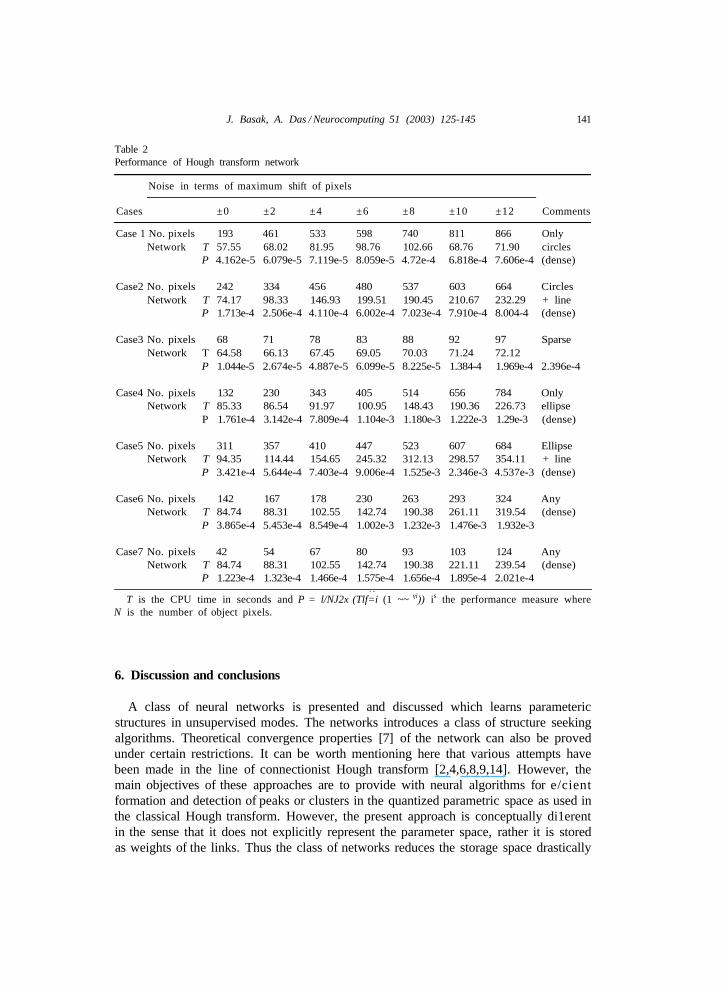
Figs. 2-9. The performance of the network is demonstrated in Table 2 for di1erentnoise amplitudes with A = 45. The performance is measured as

where u,=exp(—ui2). The performance measure indicates the fact that if a point perfectlybelongs to any one of the detected structures, i.e., vi = 1 for some i then it adds noerror. However, if it is far from all the structures, i.e., vi = 0 for all i then it adds to

J. Basak, A. Das / Neurocomputing 51 (2003) 125-145 137

Table 1Performance of the network for di1erent values of X and di1erent noise amplitudes

X

58121620

0

3.4 x 10-'3.7 x 10-4

3:08 x 10-5

5:26 x 10-6

1:04 x 10-5

1

0.00670.00920.01040.00900.0087

2

0.03040.04700.04420.03330.0285

3

0.05690.06790.06600.06080.0578

4

0.08540.08150.08180.10060.0952

Performance indicates the error or impreciseness in detecting the structures and is given as Perf =l/NJ2x EL (1 ~~ vi(x)) where vi = 1=(1 + (ui=5)2) such that Perf depends only on the error or impre-ciseness and independent on the selection of X.

20 40 60 80 100 120 140 40 60 80# Iterations-*

Fig. 3. Case 1.

20

40

60

80

100

120

140

^ v i

20 40 60 80 100 120 140 10 20 30 40 50 60 70 80 90# Iterations^

Fig. 4. Case 2.

138 J. Basak, A. Das / Neurocomputing 51 (2003) 125-145

20

40

60

80

100

120

140

0 20 40 60 80 100 120 140 160_5.5

100 200 300 400 500 600 700 800# Iterations>

Fig. 5. Case 3.

20 40 60 80 100 120 140 10 15 20 25 30 35

# Iterations ->

40 45

Fig. 6. Case 4.

the error. Essentially, P represents a kind of impreciseness or 1 — P reOects the extentor accuracy to which the network has detected the structure. If the data is noisy thenP will be large. In order to get uniformity between situations having sparse and densedata sets, the measure is normalized by the total number of data points.

It may be noted here that during convergence, the network may encounter certaindi/culties in obtaining the desired solution. First of all, the selection of X sometimesplays an important role. If X is selected very small then the network does not convergeat all. However, for wide range of X (10-50), the performance of the network remainssatisfactory and also it depends on the size of the image. We noted that it is better toselect a larger value for X initially and then towards the convergence, the value of X canbe reduced to order to obtain the proper localization of the structures. The performanceof the network also deteriorates if the number of output nodes is not selected properly.

J. Basak, A. Das / Neurocomputing 51 (2003) 125-145 139

OUTPUT OF HOUGH TRANSFORM NETWORK

0 20 40 60 80 100 120 140 160

20

40

60

80

100

120

140

K / 7^ \ \ ^ / jj

20 40 60 80 100 120 140

20 40 60 80 100 120 140 160 180

# Iterations>

Fig. 7. Case 5.

20 40 60 80 100 120 140 160 180# Iterations ->

Fig. 8. Case 6.

If it is more than the desired number of nodes then it is not very harmful (within acertain limit) because multiple nodes converge to the same solution. If the number ofnodes is less than the desired one then the network converges to some spurious solutionswith average e1ect from di1erent structures. Interference between di1erent structures(particularly, the second order structures) poses another problem in the identi2cation.It is found that if a small circle of ellipse segment is placed close to another largecircular or elliptical or linear segment (having a large count of data points) then theidenti2ed smaller structure is dragged towards the larger one.

5.3. E:ectiveness in real-life images

The e1ectiveness of the network has also been tested in detecting structures fromreal-life images. It may be mentioned here that a number of attempts have been made

140 J. Basak, A. Das / Neurocomputing 51 (2003) 125-145

50 100 150 200 250 300 350 400 450 500# Iterations-*

Fig. 9. Case 7.

20 40 60 80 100 120 140 (b)

Fig. 10.

20 40 60 SO 100 120 140

to extract elliptical structures from real-life images using di1erent variations of Houghtransform. In most of these approaches special algorithms and techniques (e.g., useof directional information, clustering in the quantized parameter space) techniques areemployed to obtain proper parametric structural descriptions and reduce spurious de-tection. In this section, we provide a set of results illustrating the structures identi2edby the proposed network from the real-life images without incorporating any domainknowledge. Figs. 10-12 illustrate structures identi2ed from the gray images after edgepoint detection. As discussed before, the results reveal the fact that in the presence ofa large number of structures, the network encounters localization problem. However,with a sparse data set or less number of structures the problem of interference getshighly reduced and the structures are properly identi2ed.

J. Basak, A. Das / Neurocomputing 51 (2003) 125-145 141

Table 2Performance of Hough transform network

Noise in terms of maximum shift of pixels

Cases ±0 ±2 ±4 ±6 ±8 ±10 ±12 Comments

Case 1 No. pixels 193 461 533 598 740 811 866 OnlyNetwork T 57.55 68.02 81.95 98.76 102.66 68.76 71.90 circles

P 4.162e-5 6.079e-5 7.119e-5 8.059e-5 4.72e-4 6.818e-4 7.606e-4 (dense)

Case2 No. pixels 242 334 456 480 537 603 664 CirclesNetwork T 74.17 98.33 146.93 199.51 190.45 210.67 232.29 + line

P 1.713e-4 2.506e-4 4.110e-4 6.002e-4 7.023e-4 7.910e-4 8.004-4 (dense)

Case3 No. pixels 68 71 78 83 88 92 97 SparseNetwork T 64.58 66.13 67.45 69.05 70.03 71.24 72.12

P 1.044e-5 2.674e-5 4.887e-5 6.099e-5 8.225e-5 1.384-4 1.969e-4 2.396e-4

Case4 No. pixels 132 230 343 405 514 656 784 OnlyNetwork T 85.33 86.54 91.97 100.95 148.43 190.36 226.73 ellipse

P 1.761e-4 3.142e-4 7.809e-4 1.104e-3 1.180e-3 1.222e-3 1.29e-3 (dense)

Case5 No. pixels 311 357 410 447 523 607 684 EllipseNetwork T 94.35 114.44 154.65 245.32 312.13 298.57 354.11 + line

P 3.421e-4 5.644e-4 7.403e-4 9.006e-4 1.525e-3 2.346e-3 4.537e-3 (dense)

Case6 No. pixels 142 167 178 230 263 293 324 AnyNetwork T 84.74 88.31 102.55 142.74 190.38 261.11 319.54 (dense)

P 3.865e-4 5.453e-4 8.549e-4 1.002e-3 1.232e-3 1.476e-3 1.932e-3

Case7 No. pixels 42 54 67 80 93 103 124 AnyNetwork T 84.74 88.31 102.55 142.74 190.38 221.11 239.54 (dense)

P 1.223e-4 1.323e-4 1.466e-4 1.575e-4 1.656e-4 1.895e-4 2.021e-4

T is the CPU time in seconds and P = l/NJ2x (Tlf=i (1 ~~ vi)) is the performance measure whereN is the number of object pixels.

6. Discussion and conclusions

A class of neural networks is presented and discussed which learns parametericstructures in unsupervised modes. The networks introduces a class of structure seekingalgorithms. Theoretical convergence properties [7] of the network can also be provedunder certain restrictions. It can be worth mentioning here that various attempts havebeen made in the line of connectionist Hough transform [2,4,6,8,9,14]. However, themain objectives of these approaches are to provide with neural algorithms for e/cientformation and detection of peaks or clusters in the quantized parametric space as used inthe classical Hough transform. However, the present approach is conceptually di1erentin the sense that it does not explicitly represent the parameter space, rather it is storedas weights of the links. Thus the class of networks reduces the storage space drastically

I-I. J. Basak, A. Das / Neurocomputing 51 (2003) 125-145

50 100 150 200 250 300 350

20 40 60 80 100 120 140

102030

405060

708090

100110

' • . _ . . -

r "-'•"''"•ttf5

i \ . • • •

p . •'•1.' -•'. J -_ _

1 ™* • '^n

- "3 - r- ? ?).:';,*iu5i'. -L i''' •: f'*'f' ../I7I.',:'" '

( y —

(b) 20 40 60 80 100 120 140

20 40 60 80 100 120 140

Fig. 11.

and increases in size only linearly with the increase in dimensionality or the numberof parameters.

The class of networks provide a way of visual information representation such thatif a visual object boundary is scanned and the pixels are presented to the networkinput then it will generate a spatio-temporal sequence which can be interpreted byother networks. On top of this two-layered model, certain hierarchical models can bedesigned for providing more meaning inter-relationships between di1erent structuressuch that more meaningful interpretations can be derived from spatio-temporal patternsgenerated by the network. An way of measuring the impreciseness or vagueness hasbeen discussed in this article which will provide to characterize the structures moremeaningfully as well as to decide the width of di1erent clusters. The imprecisenessmeasure can also provide a guideline for attentional mechanism [8] in generating theinterpretable spatio-temporal output from a given image with the help of such kind ofstructure seeking networks.

J. Basak, A. Das / Neurocomputing 51 (2003) 125-145 143

(a)

(c)

140

10 20 30 40 50 60 70 80 90100110

20 -

40 -

60 -

80 -

100 -

120 -

140 -\

20 0 20 40 100 120 140

(b) 10 20 30 40 50 60 70 80 9 0 1 1 0

Fig. 12.

20 0 20 40 60 80 100 120 140

Acknowledgements

The authors take the privilege to gratefully acknowledge the anonymous reviewersfor their constructive criticism and pointers to useful references.

References

[1] S. Amari, Neural theory of association and concept formation, Biol. Cyber. 26 (1977) 175-185.[2] Y. Amit, A neural network architecture for visual selection, Neural Comput. 12 (2000) 1141-1164.[3] D.H. Ballard, Generalizing the Hough transform to detect arbitrary shapes, Pattern Recognition 13

(1981) 111-122.[4] D.H. Ballard, Parameter nets, Artif. Intell. 22 (1984) 235-267.[5] D. Ballard, C. Brown, Computer Vision, Prentice-Hall Inc., Englewood Cli1s, NJ, 1982.[6] S.P. Banks, R.F. Harrison, Simple object recognition by neural networks—application of the Hough

transform, Int. J. Control 54 (1991) 1469-1476.[7] J. Basak, Learning Hough transform, Neural Comput. 13 (2001) 651-676.[8] J. Basak, S.K. Pal, PsyCOP: a psychologically motivated connectionist system for object perception,

IEEE Trans. Neural Networks 6 (1995) 1337-1354.[9] J. Basak, N.R. Pal, S.K. Pal, A connectionist system for learning and recognition of structures, Neural

Networks 8 (1995) 643-657.

144 J. Basak, A. Das / Neurocomputing 51 (2003) 125-145

[10] A.J. Bell, T.J. Sejnowski, An information maximization approach to blind separation and blinddeconvolution, Neural Comput. 7 (1995) 1129-1159.

[11] J.C. Bezdek, Pattern Recognition with Fuzzy Objective Function Algorithms, Plenum Press, New York,1981.

[12] R. Cole, J.S. Salowe, W.L. Steiger, E. Szemered, An optimal-time algorithm for slope selection, SIAMJ. Comput. 18 (1989) 792-810.

[13] G. Danuser, M. Stricker, Parametric model 2tting: from inlier characterization to outlier detection, IEEETrans. Pattern Anal. Mach. Intell. 20 (1998) 263-280.

[14] G.L. Dempsey, E.S. McVey, A Hough transform system based on neural networks, IEEE Trans. Ind.Electron. 39 (1992) 522-528.

[15] R.O. Duda, P.E. Hart, Use of Hough transform to detect lines and curves in pictures, Commun. ACM15 (1972) 11-15.

[16] S. Haykin, Neural Networks: A Comprehensive Foundation, Macmillan College Publishing Co. Inc.,New York, 1994.

[17] J. Illingworth, J. Kittler, A survey of the Hough transform, Comput. Vision, Graphics Image Process.44 (1988) 87-110.

[18] H. Kalviainen, P. Hirvonen, L. Xu, E. Oja, Probabilistic and non-probabilistic Hough transforms:overview and comparisons, Image and Vision Comput. 13 (1995) 239-252.

[19] N. Kiryati, A.M. Bruckstein, Heteloscedastic Hough transform (HtHT): an e/cient method for robustline 2tting in the 'Errors in the Variable' problem, Comput. Vision Image Understanding (CVIU) 78(2000) 69-83.

[20] V. Kyrki, H. Kalviainen, Combination of local and global line extraction, J. Real-Time Imaging JRTI6 (2000) 79-91.

[21] J. Lampinen, E. Oja, Distortion tolerant pattern recognition based on self-organizing feature extraction,IEEE Trans. Neural Networks 6 (1995) 539-547.

[22] V.F. Leavers, Which Hough transform, CVGIP: Image Understanding 58 (1993) 250-264.[23] W. Li, J.J. Swetits, The liners 1-2 estimation and the Huber M-estimator, SIAM J. Optim. 8 (1998)

457^175.[24] G.J. McLachlan, T. Krishnan, The EM Algorithm and Extensions, Wiley, New York, 1997.[25] D.M. Mount, N.S. Netanyahu, E/cient randomized algorithms for robust estimation of circular arcs and

aligned ellipses, Comput. Geometry Theory Appl. 19 (2001) 1-33.[26] E. Oja, A simpli2ed neuron model as a principal component analyzer, J. Math. Biol. 15 (1982) 267-273.[27] B.A. Olashausen, D.J. Field, Emergence of simple-cell receptive 2eld properties by learning a sparse

code for natural images, Nature 381 (1996) 607-609.[28] P.K. Sen, Estimates of the regression coe/cient based on Kandell’s tau, Amer. Statist. Assoc. J. 63

(1963) 1379-1389.[29] L. Xu, E. Oja, Curve detection by an extended self-organizing map and the related RHT method,

in: Proceedings of the International Neural Network Conference (INNC90), Paris, France, 1990,pp. 27-30.

[30] O. Yanez-Suarez, M.R. Azimi-Sadjadi, Unsupervised clustering in Hough space for identi2cation ofpartially occluded objects, IEEE Trans. Pattern Anal. Mach. Intell. 21 (1999) 946-950.

[31] H.H. Yang, S. Amari, Adaptive on-line learning algorithms for blind separation-maximum entropy andminimum mutual information, Neural Comput. 9 (1997) 1457-1482.

Anirban Das did his B.E. in Electrical Engineering, from Bengal Engineering Col-lege, Howrah, India, and M.Tech. in Computer Science from Indian Statistical Insti-tute, Calcutta, India. He worked with plant engineering division of Larsen & ToubroLtd., product security R&D division of Gemplus India Pvt. Ltd. and presently work-ing with engines and systems division of Honeywell. His current interests are digitalsignal processing, cryptography, image processing and neural network.

J. Basak, A. Das / Neurocomputing 51 (2003) 125-145 145

Jayanta Basak did B.E. (electronics and telecommunication engineering) from Ja-davpur University, Calcutta, M.E. (computer science and engineering) from IndianInstitute of Science (IISc), Bangalore, and Ph.D. from Indian Institute StatisticalInstitute (ISI), Calcutta in 1987, 1989 and 1995, respectively. He served as a com-puter engineering in the KBCS project of ISI from 1989 to 1992, and as a facultyof the same Institute from 1992 to 2000. Since 2000, he is a research sta1 mem-ber of IBM India Research Lab, Delhi. He was a visiting scientist at the RoboticsInstitute of Carnegie Mellon University during 1991-1992 (UNDP fellow) and aresearcher in the RIKEN Brain Science Institute, Japan during 1997-1998. He re-ceived young scientist award from Indian Science Congress Association (ISCA),Indian National Science Academy (INSA), International Neural Network Society

(INNS), USA n 1994, 1996 and 2000, respectively. His research interests include neural network and softcomputing, pattern recognition, vision, image processing and internet computing.