Computers & Geosciences ] (]]]]) ]]]–]]]

Contents lists available at ScienceDirect

Computers & Geosciences

0098-30

doi:10.1

$Then Corr

E-m

hussein

Pleasdime

journal homepage: www.elsevier.com/locate/cageo

HOSIM: A high-order stochastic simulation algorithm for generatingthree-dimensional complex geological patterns$

Hussein Mustapha n, Roussos Dimitrakopoulos

COSMO—Stochastic Mine Planning Laboratory, Department of Mining and Materials Engineering, McGill University, 3450 University St., Montreal, Que., Canada H3A 2A7

a r t i c l e i n f o

Article history:

Received 15 April 2010

Received in revised form

26 August 2010

Accepted 7 September 2010

Keywords:

Sequential simulation

High-order spatial cumulants

Legendre polynomials

04/$ - see front matter & 2010 Elsevier Ltd. A

016/j.cageo.2010.09.007

code will be available at http://cosmo.mcgill

esponding author.

ail addresses: hussein.mustapha@mcgill.ca,

_mustapha@hotmail.com (H. Mustapha).

e cite this article as: Mustapha, H., Dinsional complex geological patterns

a b s t r a c t

The three-dimensional high-order simulation algorithm HOSIM is developed to simulate complex non-

linear and non-Gaussian systems. HOSIM is an alternative to the current MP approaches and it is based

upon new high-order spatial connectivity measures, termed high-order spatial cumulants. The HOSIM

algorithm implements a sequential simulation process, where local conditional distributions are

generated using weighted orthonormal Legendre polynomials, which in turn define the so-called

Legendre cumulants. The latter are high-order conditional spatial cumulants inferred from both the

available data and training images. This approach is data-driven and reconstructs both high and lower-

order spatial complexity in simulated realizations, while it only borrows from training images

information that is not available in the data used. However, the three-dimensional implementation of

the algorithm is computationally very intensive. To address his topic, the contribution of high-order

conditional spatial cumulants is assessed in this paper through the number of Legendre cumulants with

respect to the order of approximation used to estimate a conditional distribution and the number of data

used within the respective neighbourhood. This leads to discarding the terms of Legendre cumulants with

negligible contributions and allows an efficient simulation algorithm to be developed. The current version

of the HOSIM algorithm is several orders of magnitude faster than the original version of the algorithm.

Application and comparisons in a controlled environment show the excellent performance and efficiency

of the HOSIM algorithm.

& 2010 Elsevier Ltd. All rights reserved.

1. Introduction

The quantification of spatial uncertainty in the characteristics of adiversity of natural phenomena is typically based upon the stochasticsimulation of stationary and ergodic random fields conditional toavailable data and information. Since the 1990s, several new simula-tion frameworks have been developed to address the limits ofwell known conventional simulation methods (e.g. Rosenblatt,1985; Journel and Alabert, 1989; Journel, 1994; Goovaerts, 1998;Tjelmeland, 1998; Chil�es and Delfiner, 1999; Bernardeau et al., 2002;Deutsch, 2002; Dimitrakopoulos and Luo, 2004; Remy et al., 2009).These limits include their ineffectiveness in dealing with spatialcomplexity, largely because they are also limited to the two-point orsecond-order spatial statistical moments of the corresponding ran-dom field models employed. New simulation frameworks andapproaches include: the multiple point simulation algorithms, suchas the snesim (Strebelle, 2002), filtersim (Zhang et al., 2006; Wu et al.,2008), and simpat (Arpat and Caers, 2007), and others such as (DeVries et al., 2008; Chiginova and Hu, 2008; Mehrdad and Caers, 2010);

ll rights reserved.

.ca.

mitrakopoulos, R., HOSIM: A. Computers and Geoscienc

Markov random field models based multipoint type approaches (Daly,2004; Tjelmeland and Eidsvik, 2004), new kernel based approaches(Scheidt and Caers, 2009); multi-scale simulations based on discretewavelet decomposition (Gloaguen and Dimitrakopoulos, 2009;Chatterjee et al., in press). Vargas-Guzman (2008, 2009) has usedcumulants to account for high-order residual terms in permeabilityestimation and for resources-in-place calculations, although thetechnical aspect of the related work is incomplete. Recently, high-order spatial cumulants were also introduced as a means to con-sistently describe complex spatial architectures and configurations(Dimitrakopoulos et al., 2010). High-order cumulants are combina-tions of moment statistical parameters characterizing non-Gaussianrandom variables (Billinger and Rosenblatt, 1966). Nikias andPetropulu (1993) provide new definitions and terms, in a systematicway, for signal processing approaches that are widespread in thesignal processing literature, including the use of high-order multi-variate cumulants for identification of noisy closed loop systems(Delopoulos and Giannakis, 1996) and in non-linear signal processing(Zhang, 2005). For more details, we refer to (Dimitrakopoulos et al.,2010). In the context of spatial random fields, the first and secondorder cumulants are but the well known mean and covariance; ingeneral, spatial cumulants may be seen as an extension of the well-known covariance function. The systematic definitions non-Gaussianspatial random fields and their high-order spatial statistics are given

high-order stochastic simulation algorithm for generating three-es (2010), doi:10.1016/j.cageo.2010.09.007

x0

x1

x2

x3

x4

Ω

xn

xi

Fig. 1. An unknown value is at the location x0 and values at the locations x1, x2,y,xn

in a neighbourhood of x0 are assumed to be known.

H. Mustapha, R. Dimitrakopoulos / Computers & Geosciences ] (]]]]) ]]]–]]]2

in Dimitrakopoulos et al. (2010) and the algorithm to efficientlycalculate high-order spatial cumulants and related source code aredetailed in Mustapha and Dimitrakopoulos (2010a). A related findingrelated to the information described by cumulants, from the abovework, is that spatial cumulants of orders three to five capturedirectional multiple point-periodicity, as well as multiple pointconnectivity including connectivity of extreme values, in additionto geometric characteristics and spatial architectures in two- andthree-dimensional datasets.

The stochastic simulation based on high-order spatial cumulants forcontinuous variables is developed in Mustapha and Dimitrakopoulos(2010b), and it is founded upon a sequential framework, where anonparametric Legendre polynomial series approximation (Lebedev,1965) is used to estimate local conditional densities. The estimation ofthese conditional densities is based on coefficients calculated in termsof spatial high-order cumulants and make no distributional assump-tions or require data transformations before and after simulating, whileworking well for complex non-Gaussian and non-linear system. Animportant aspect of this new framework, as shown in the abovereference, is that the specific relations between the order of the spatialcumulants and the lower order moments, as it exists in the datasetused, are maintained by the simulated realizations. This makes thesimulation process consistent over a series of orders, that is, spatialcumulants are not some randomly selected moments. This is also amain difference with the existing multiple point methods (Boucher,2009) and leads to realizations where all the lower order statistics in adataset is reproduced, something that the existing multipoint methodsdo not ensure, thus conflicts appear when the number of hard dataincreases (Strebelle, 2002). Note that existing multiple point methodsreproduce the statistics of the training image employed. Despite theadvantages shown in past work, simulation based on high-order spatialcumulants is computationally demanding, particularly as the numberof dimensions considered increases. This is the area where thismanuscript contributes by assessing the contribution of various termsof Legendre polynomials so as to reduce computational needs withoutloss of important information as well as providing a full three-dimensional algorithm for the practical use of the method in variousapplications.

In the following sections, firstly, the sequential simulation methodusing high-order spatial conditional cumulants is reviewed and therelated general algorithm (HOSIM) introduced; the computationalcomplexity and sensitivities of this algorithm are also presented andexplored in some detail. Then, the specifics input parameters forHOSIM are described. Subsequently, applications show how HOSIMperforms using different options, and conclusions follow.

2. The HOSIM algorithm and related computations aspects

The proposed HOSIM algorithm (Mustapha and Dimitrakopoulos,2010b) proceeds in two steps: (1) cumulants calculation and (2)sequential simulation. HOSIM first calculates cumulants of differentorder using template data obtained from scanning a training image(TI) and available data. Next, the grid points are simulated sequen-tially using a non-parametric method based on Legendre polynomialswith coefficients calculated from the cumulant maps in (1).

2.1. High-order cumulants

Cumulants are obtained by scanning TIs and available data asshown in Dimitrakopoulos et al. (2010). The algorithm used toaccomplish this stage is based on HOSC algorithm developed inMustapha and Dimitrakopoulos (2010a).

Denote by x0 an unsampled location subject to simulation usinga set of its closer neighbours as shown in Fig. 1. The spatialcorrelation between variable Z0 defined at x0 and two random

Please cite this article as: Mustapha, H., Dimitrakopoulos, R., HOSIM: Adimensional complex geological patterns. Computers and Geoscienc

variables Zi, Zj defined, respectively, at neighbours xi, xj is expressedusing a third-order cumulant cum(Z0, Zi, Zj). Assuming that Z0, Zi andZj are zero-mean random variables, then cum(Z0, Zi, Zj), identified asbivariate distance function cum(h1,h2), is calculated as

cumðh1, h2Þ ¼1

Nh1 ,h2

XNh1 ,h2

k ¼ 1

ZðxkÞZðxkþh1ÞZðxkþh2Þ,

fxk; xkþh1; xkþh2gATh1 ,h2

3 , ð1Þ

where Th1 ,h2

3 is the associated spatial template of order 3 and isdefined (considering a spatial location x as a reference) as

Th1 ,h2

nþ1 ðh1,h2,a1,a2Þ ¼ fðx,xþh1,xþh2Þsuch that the points

fx,xþhi, i¼ 1,2g are a set of the original

points distributiong ð2Þ

In Eq. (2), distances h1 and h2 are directed along two directionsf d!

i, i¼ 1,2g that are supported by the direction angles {a1, a2}.Finally, the elements in Th1 ,h2

3 are searched from the TI and availabledata. The fourth-order cumulant, expressed as a trivariate distancefunction cum(h1,h2,h3), is calculated using template Th1 ,h2 ,h3

4 as

cumðh1,h2,h3Þ ¼1

Nh1 ,h2 ,h3

XNh1 ,h2 ,h3

k ¼ 1

ZðxkÞZðxkþh1ÞZðxkþh2ÞZðxkþh3Þ

�1

ðNh1 ,h2 ,h3Þ2

XNh1 ,h2 ,h3

k ¼ 1

ZðxkÞZðxkþh1Þ

0@

1A

24

�XNh1 ,h2 ,h3

k ¼ 1

Zðxkþh2ÞZðxkþh3Þ

0@

1A35

�1

ðNh1 ,h2 ,h3Þ2

XNh1 ,h2 ,h3

k ¼ 1

ZðxkÞZðxkþh2Þ

0@

1A

24

�XNh1 ,h2 ,h3

k ¼ 1

Zðxkþh1ÞZðxkþh3Þ

0@

1A35

�1

ðNh1 ,h2 ,h3Þ2

XNh1 ,h2 ,h3

k ¼ 1

ZðxkÞZðxkþh3Þ

0@

1A

24

�XNh1 ,h2 ,h3

k ¼ 1

Zðxkþh1ÞZðxkþh2Þ

0@

1A35

fxk; xkþh1; xkþh2; xkþh3gATh1 ,h2 ,h3

4 ð3Þ

where Nh1,h2 and Nh1,h2,h3 are the number of elements of Th1 ,h2

3 andTh1 ,h2 ,h2

4 , respectively. Cumulants of order higher than four are

high-order stochastic simulation algorithm for generating three-es (2010), doi:10.1016/j.cageo.2010.09.007

Table 1HOSIM algorithm for 2D continuous variable simulations.

MAX 0 1 2 3

Ncoeff 1 7 28 84

H. Mustapha, R. Dimitrakopoulos / Computers & Geosciences ] (]]]]) ]]]–]]] 3

similarly calculated. For more details, we refer to Appendix A andreferences therein.

2.2. Sequential simulation

HOSIM utilizes the classic sequential simulation paradigm(Deutsch and Journel, 1998). At each node x along the randompath visiting the simulation grid, a search template TEMP is used toextract the conditioning data event. The conditional probabilitydensity function is estimated using series of Legendre polynomialsand coefficients expressed in terms of cumulants.

Consider a stationary and ergodic random field Z(xi) or Zi,xiAODRr (r¼1, 2 or 3) for i¼0,y, N, where N is the number ofpoints in a discrete grid (DN) and a set of conditioning datadn¼{Z(xa), a¼1,..., n}.

Assume that x0 is the first node visited and its neighbours arefound within a certain neighbourhood (Fig. 1). The HOSIM algorithmcalculates the conditional probability density function (cpdf) fZ0 givendn using cumulants maps and Legendre polynomials as the following:

fZ0ðz0=dnÞ ¼

1RDfZðxÞdz0

fZðz0, z1,. . ., znÞ

¼1R

DfZðxÞdz0

X1i0 ¼ 0

. . .X1

iN�1 ¼ 0

X1iN ¼ 0

Li0 ,i1 ,...,iN�1 ,iN Pi0 ðz0Þ ð4Þ

where Pm the normalized Legendre polynomials defined as Pm ðzÞ ¼ffiffiffiffiffiffiffiffiffiffiffiffiffiffiffi2mþ1p

PmðzÞ=ffiffiffi2p

, Li0 ,...,iN�1 , iN ¼ Li0 ,...,iN�1 ,iN Pi1 ðz1Þ. . .PiN�1ðzN�1ÞPiN ðzNÞ

and Li0 ,...,iN�1 ,iN

are defined in terms of cumulants as shown inMustapha and Dimitrakopoulos (2010b) and Appendix B. Here, wenote that {z1,y, zn} are the values of the samples around x0.

2.3. The complexity of the HOSIM algorithm

2.3.1. Current computational complexity

Legendre series coefficients Li0 ,...,iN�1 ,iN

, usually called Legendrecumulants, of order smaller than or equal to o are only used; thenthe density function fZ0

in Eq. (1) can be approximated as follows:

fZ0ðz0=dnÞ ¼

1RDfZðxÞdz0

fZðz0, z1, . . ., znÞ � f Z0 ,oðz0=dnÞ

¼1R

DfZðxÞdz0

Xoi0 ¼ 0

. . .XiN�2

iN�1 ¼ 0

XiN�1

iN ¼ 0

Li0 , i1 ,:::, iN�1 , iN

Pi0 ðz0Þ ð5Þ

where ik ¼ ik�ik�1 for koN. The coefficients Li1 ,...,iN�1 ,iN

are functionsof spatial cumulants, as explained earlier, and are inferred from TI

Fig. 2. Variation of Ncoeff with respect to o (i.e. N¼5 is fixed

Please cite this article as: Mustapha, H., Dimitrakopoulos, R., HOSIM: Adimensional complex geological patterns. Computers and Geoscienc

and samples as presented in Mustapha and Dimitrakopoulos(2010b).

The variation of the number of Legendre cumulants, Ncoeff, to becalculated with respect to: (1) the order of approximationo and (2)the number of neighbours considered to simulate a visiting node isstudied in this section. The number of terms involved in Eq. (5) isequal to

Ncoeff ¼ðoþ1Þðoþ2Þ. . .ðoþNþ1Þ

ðNþ1Þ!ð6Þ

For example, Ncoeff¼28 for an order o¼2 and a number ofsamples N¼5; the variations of Ncoeff, respectively, with respect too for a fixed N, and with respect to N for a fixed o are shown inFig. 2. Reducing Ncoeff with an appropriate method is discussed next.

2.3.2. Reducing computational complexity

The Legendre polynomials are defined on ]�1,1[; then themoments (or cumulants) EðZi1

0 Zi21 . . .Z

ikk Þ can be neglected for i0,

i1,y,ik4MAX, where MAX is a number higher than 1 becauseEðZi1

0 Zi21 . . .Z

ikk Þ-0. Table 1 shows the variation of Ncoeff with respect

to MAX for fixed o¼3 and N¼5. A way of reducing the number ofterms consists of only calculating explicitly seven cumulants toestimate the conditional density in Eq. (5). For N¼10, only 11 termsare needed. Then, at most (N+2) terms are calculated for N numberof samples used to simulate a value at x0.

For N¼5, the seven coefficients to be calculated are

) in (1) and

high-ordes (2010)

with respect to N (i.e. o¼3 is fix

er stochastic simulation alg, doi:10.1016/j.cageo.2010.0

ed) in (2)

orithm9.007

(1)

cumðZ00 ,Z0

1 ,. . .,Z0k Þ,

(2) cumðZ1

0 Þ,

(3)

cumðZ10 , Z1

1Þ,

(4) cumðZ10 ,Z1

1 ,Z12Þ,

(5)

cumðZ10 ,Z1

1 ,Z12 ,Z1

3Þ,

(6) cumðZ10 ,Z1

1 ,Z12 ,Z1

3 ,Z14Þ,

(7)

cumðZ10 ,Z1

1 ,Z12 ,Z1

3 ,Z14 ,Z1

5Þ.

The coefficient (3) represents the covariance between Z0 and Z1;the covariance between Z0 and Z2 is implicitly included in the third-order cumulant, i.e. coefficient (4). Similarly, for the covariancebetween Z0 and Zi, i¼3–5. The third-order cumulant of Z0, Z1, Z2 isgiven by coefficient (4); however, the third-order cumulants of Z0 andany other two variables Zi, Zj, i,j¼1–5 are considered in the higherorder cumulants. Then, coefficients (1)–(7) cover the correlations

.

for generating three-

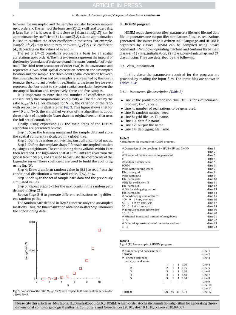
Table 2A parameter file example of HOSIM program.

# Dimension of the problem: 1¼1D, 2¼2D and 3¼3D -Line 1

3 -Line 2

# Number of realizations to be generated -Line 3

5 -Line 4

#Random number seed -Line 5

90054 -Line 6

#File with training image -Line 7

File_name.grid -Line 8

#File with data -Line 9

File_name.data -Line 10

#File for realization (S) -Line 11

File_name.out -Line 12

# File for debugging output -Line 13

File_name.dbg -Line 14

# Coordinate system of the TI -Line 15

100 0 1 # nx, xmn, xsiz -Line 16

50 0 1 # ny, ymn, ysiz -Line 17

30 0 1 # nz, zmn, zsiz -Line 18

# Template search dimensions -Line 19

10 5 5 -Line 20

H. Mustapha, R. Dimitrakopoulos / Computers & Geosciences ] (]]]]) ]]]–]]]4

between the unsampled and the samples and also between samplesup to order six. The terms of the form cumðZn0

0 ,Z11Þwill tend to zero if n0

is large (i.e. b1); however, if n0 is close to 1 than, cumðZn0

0 ,Z11 Þ can be

approximated by coefficient (3), i.e. cumðZ10 ,Z1

1Þ. Same approximationis used to calculate the other coefficient in the series. For example,cumðZn0

0 ,Zn1

1 ,Z12Þ may tend to zero or to cumðZ1

0 ,Z11 ,Z1

2 Þ, i.e. coefficient(4), depending on the values of n0 and n1.

The set of (N+2) cumulants represents a basis for all spatialcorrelations up to order 6. The first two terms represent the integral ofthe density (cumulant of order zero) and the mean (cumulant of orderone). The third term (cumulant of order two) is the covariance andrepresents a two-point spatial correlation between the unsampledlocation and one sample. The three-point spatial correlation betweenthe unsampled location and two samples is represented by the fourthterm, i.e. the cumulant of order three. Similarly, the terms five to sevenrepresent the four-point to six-point spatial correlation between theunsampled location and, respectively, three and five samples.

It is important to note that the number of coefficients andconsequently the computational complexity will be reduced by theratio Ncoeff/(N+2). For example for N¼5, the variation of the ratiowith respect to o is illustrated in Fig. 3. This figure shows that foro¼10 and N¼5, the simplified version of the algorithm is aboutthree orders of magnitude faster than the original version that usesthe full set of cumulants.

Finally, using expression (2), the main steps of the HOSIMalgorithm are presented below:

Step 1: Scan the training image and the sample data and storethe spatial cumulants calculated in a global tree.

Step 2: Define a random path visiting once all unsampled nodes.Step 3: Define the template shape T for each unsampled location

x0 using its neighbours. The conditioning data available within T arethen searched. The high-order spatial cumulants are read from theglobal tree in Step 1, and are used to calculate the coefficients of theLegendre series. These coefficient are used to build the cpdf of Z0

using Eq. (5).Step 4: Draw a uniform random value in [0,1] to read from the

conditional distribution a simulated value, Z(x0), at x0.Step 5: Add x0 to the set of sample hard data and the previously

simulated values.Step 6: Repeat Steps 3–5 for the next points in the random path

defined in Step (2).Repeat Steps 2–6 to generate different realizations using differ-

ent random paths.The random path defined in Step 2 concerns only the unsampled

locations. Thus, the final realization obtained in after Step 6 honoursthe conditioning data.

Fig. 3. Variation of the ratio Ncoeff/(N+2) with respect to the order of the serieso for

a fixed N¼5.

Please cite this article as: Mustapha, H., Dimitrakopoulos, R., HOSIM: Adimensional complex geological patterns. Computers and Geoscienc

3. HOSIM program

HOSIM reads three input files: parameters file, grid file and datafile; it generates one output file: simulations files, i.e. realizationsgenerated. The source code is written in C++language, and HOSIM isorganized by classes. HOSIM can be compiled using nmake

command in Windows operating machine and contains three mainclasses: (1) class_initialization, (2) class_cumulants_map and (3)class_hosim. They are described by the following.

3.1. class_initialization

In this class, the parameters required for the program areprovided by reading the input files. The input files are shown inTables 2–4:

3.1.1. Parameters file description (Table 2)

�

#

4

#

3

TabA g

#

1

#

^

1

hies (

Line 2: the problem dimension Dim. Dim¼k for k-dimensional

problem, k¼1, 2, or 3.

� Line 4: number of realizations to be generated. � Line 6: random number seed. � Line 8: grid file, i.e. TI, name. � Line 10: data file name. � Line 12: output file name. � Line 14: debugging file name.

Minimal & maximal number of neighboors -Line 21

5 -Line 22

Order of approximation of the series and max -Line 23

3 -Line 24

le 3rid (TI) file example of HOSIM program.

Number of grid nodes in the TI -Line 1

50,000 -Line 2

For each grid node:

ind, x, y, z and value

-Line 3

1 1 1 1 4.06 -Line 4

2 2 1 1 2.95 -Line 5

3 3 1 1 4.34 -Line 6

4 4 1 1 5.48 -Line 7

5 5 1 1 5.64 -Line 8

^ ^ ^ ^ -Line 9

-Line 10

-Line 11

50,000 100 50 30 2.34 -Line 12

gh-order stochastic simulation algorithm for generating three-2010), doi:10.1016/j.cageo.2010.09.007

H. Mustapha, R. Dimitrakopoulos / Computers & Geosciences ] (]]]]) ]]]–]]] 5

The coordinate system of the TI is defined by specifying thecenter coordinates of the first, i.e. the lower left point (xmn, ymn,zmn), the number of grid nodes (nx, ny, nz), and the spacing of thenodes (xsiz, ysiz, zsiz).

�

TabA d

#

9

#

1

2

3

4

5

6

7

8

9

F

Pd

Line 16: (nx, xmn, xsiz) the grid, i.e. TI, definition in thex-direction.

� Line 17: (ny, ymn, ysiz) the grid definition in the y-direction. � Line 18: (nz, zmn, zsiz) the grid definition in the z-direction. � Line 20: template search dimensions. In the current version of

HOSM, the template is a 2D and/or 3D rectangle.

� Line 22: minimal and maximal number of neighbours to

simulate a visiting node.

� Line 24: order of approximation o of Legendre series, and the

term MAX defined in Section 2.3.

le 4ata file example of HOSIM program.

Number of samples in the data file -Line 1

-Line 2

For each sample: ind, x, y, z and value -Line 3

10 12 3 -Line 4

14 16 25 -Line 5

8 6 17 -Line 6

22 33 2 -Line 7

55 5 12 -Line 8

87 7 3 -Line 9

75 41 23 -Line 10

62 15 15 -Line 11

33 9 7 -Line 12

Training image Samples

Fig. 4. (1) Training image; hard data locations in (2).

ig. 5. Simulation of a 3D fluvial reservoir: (1) Exhaustive image: true image (390,00

lease cite this article as: Mustapha, H., Dimitrakopoulos, R., HOSIM: Aimensional complex geological patterns. Computers and Geoscienc

3.1.2. Grid file description (Table 3)

The grid file contains the Training Image (TI) which is assumedto be a 2D or 3D rectangle with values defined at a regular grid asshown in Fig. 4(1). This file is described as

�

0 p

hies (

Line 2: total number of nodes (NN) used in the TI geometrydescription.

� Lines 7-end of file: nodes information. For each node

p(p¼1,y,NN), we provide its coordinates Xp, Yp, Zp and, V[p],the value at p. For 2D problem Zp is zero.

3.1.3. Data file description (Table 4)

The data file contains the samples (Fig. 4(2)) information. It isdescribed as follows:

�

Line 2: total number of samples (NS). � Lines 4–12: samples information. For each sample s

(p¼1,y,NS), we provide its coordinates Xs, Ys, Zs and, V[s],the value at p. For 2D problem Zs is zero.

3.2. class_cumulants_map

Given the order of the series and the template size, this classcalculates all cumulants required in expression (2) as detailed inSection 2.1. The cumulants are calculated using TIs and data. Globalmaps are used to store the cumulant coefficients. The algorithmused in this part is inspired from HOSC algorithm developed byMustapha and Dimitrakopoulos (2010a).

3.3. class_hosim

This class is the main part of the program. It uses the cumulantsmaps calculated in the previous class and the expression (2) tocalculate the conditional PDF at each visited node.

4. Numerical results

A three-dimensional image of channels of different sizes(Fig. 5(1)) is considered and it is used here to provide an insightto simulations and interpretations of HOSIM in three dimensions.This image shows the porosity variation in a 100�130�30 m3

field. The data set used (syn_poro.out) are available in the Stanford VReservoir Data Set (Mao and Journel, 1999). Fig. 5(1) shows theexhaustive image to be simulated from the sample data set (DS) inFig. 5(2). DS is combined with the training image (Mustapha andDimitrakopoulos, 2010b) to infer the high-order spatial cumulants

oints) and (2) DS: 500 sample data (E0.13% of the total number of points).

gh-order stochastic simulation algorithm for generating three-2010), doi:10.1016/j.cageo.2010.09.007

H. Mustapha, R. Dimitrakopoulos / Computers & Geosciences ] (]]]]) ]]]–]]]6

that are needed for the estismation of the local pdfs. Fig. 5(1) is usedas a TI in this example. Sensitivity analysis of HOSIM to the TIs used,unconditional realizations and comparisons with other algorithmsare shown in Mustapha and Dimitrakopoulos (2010b).

The full set and truncated set of cumulants, discussed above, areboth employed to generate five realizations generated using HOSIMwhere about 14 nearby data are selected in average for the simulationof any single node. The main features of our approach are illustratedthrough the following discussion. All runs are performed on a 3.2 GHzIntel(R) Xeon (TM) PC with 2 GB of RAM.

The case of full set is compared to truncated set by simulating theexhaustive data set shown in Fig. 5(1) using the data set (DS) inFig. 5(2). Realizations using the two sets of cumulants are gener-ated with the same seed number as shown in Fig. 6. The figureshows similar results. Fig. 7 shows that histogram and variogramsof the samples are well reproduced by both realizations. High-orderstatistics of the samples are also reproduced by HOSIM realizationsas shown by third- and fourth-order cumulants in Figs. 8 and 9.

Fig. 10 compares two cross-sections along z (Fig. 10—firstcolumn) of the exhaustive image to corresponding cross-sections(Fig. 10—second column, —third column) of two HOSIM realiza-tions generated using the truncated set. The figure shows a goodreproduction of the channels in the exhaustive image. The

Fig. 6. A realization generated by HOSIM using DS by calculating (1) explicitly full set

Fig. 7. Histograms (1), variograms (2–4) of two HOSIM realizations using truncated and

realizations.

Please cite this article as: Mustapha, H., Dimitrakopoulos, R., HOSIM: Adimensional complex geological patterns. Computers and Geoscienc

statistics, i.e. histograms, variograms and high-order cumulants,of the realizations and samples are very close as shown in Figs. 11–13. Finally, it is important to note that the results presented in thissection are calculated with very small number of terms and are verygood comparing to the results obtained by using the full set ofcumulant terms. In addition, the algorithm is not sensitive to theMAX variable. In contrast, very appropriate results are obtained byworking only with few cumulant terms.

5. Conclusions

A 3D stochastic simulation method (HOSIM) has been presentedand it is conceived for simulating complex geological patterns. Themethod developed uses high-order Legendre polynomials withcoefficient calculated from cumulants population. The HOSIMalgorithm is validated by simulating a three-dimensional domainof complex channels. In addition, the computational costs of HOSIMare discussed. A method to reduce HOSIM’s complexity is presentedwhere only aulated; the other cumulants are inferred from thereference subset using the convergence property of the sequ themodified algorithm is several orders of magnitude faster than theoriginal version of the algorithm that calculates explicitly all spatial

of terms and (2) only use truncated set of (N+2) terms discussed in Section 2.3.

full set of cumulants, respectively. Circles refer to data set and the solid lines refer to

high-order stochastic simulation algorithm for generating three-es (2010), doi:10.1016/j.cageo.2010.09.007

Fig. 8. Third-order cumulant maps of DS (1,4,7) and two HOSIM realizations using truncated set of cumulants (2,5,8) and full set of cumulants (3,6,9), respectively.

Fig. 9. Fourth-order cumulant maps of DS (1) and two HOSIM realizations using truncated set of cumulants (2) and full set of cumulants (3), respectively.

H. Mustapha, R. Dimitrakopoulos / Computers & Geosciences ] (]]]]) ]]]–]]] 7

Please cite this article as: Mustapha, H., Dimitrakopoulos, R., HOSIM: A high-order stochastic simulation algorithm for generating three-dimensional complex geological patterns. Computers and Geosciences (2010), doi:10.1016/j.cageo.2010.09.007

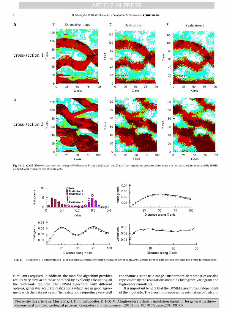
Fig. 10. (1a) and (1b) two cross-sections along z of exhaustive image and (2a, 2b) and (3a, 3b) corresponding cross-sections along z in two realizations generated by HOSIM

using DS and truncated set of cumulants.

Fig. 11. Histograms (1), variograms (2–4) of five HOSIM realizations using truncated set of cumulants. Cercles refer to data set and the solid lines refer to realizations.

H. Mustapha, R. Dimitrakopoulos / Computers & Geosciences ] (]]]]) ]]]–]]]8

cumulants required. In addition, the modified algorithm providesresults very similar to those obtained by explicitly calculating allthe cumulants required. The HOSIM algorithm, with differentoptions, generates accurate realizations which are in good agree-ment with the data set used. The realizations reproduce very well

Please cite this article as: Mustapha, H., Dimitrakopoulos, R., HOSIM: Adimensional complex geological patterns. Computers and Geoscienc

the channels in the true image. Furthermore, data statistics are alsoreproduced by the realizations including histogram, variogram andhigh-order cumulants.

It is important to note that the HOSIM algorithm is independentof the input info. The algorithm requires the estimation of high and

high-order stochastic simulation algorithm for generating three-es (2010), doi:10.1016/j.cageo.2010.09.007

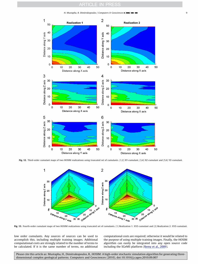
Fig. 12. Third-order cumulant maps of two HOSIM realizations using truncated set of cumulants. (1,2) XY-cumulant, (3,4) XZ-cumulant and (5,6) YZ-cumulant.

Fig. 13. Fourth-order cumulant maps of two HOSIM realizations using truncated set of cumulants. (1) Realization 1: XYZ-cumulant and (2) Realization 2: XYZ-cumulant.

H. Mustapha, R. Dimitrakopoulos / Computers & Geosciences ] (]]]]) ]]]–]]] 9

low order cumulants. Any sources of sources can be used toaccomplish this, including multiple training images. Additionalcomputational costs are strongly related to the number of terms tobe calculated. If it is the same number of terms, no additional

Please cite this article as: Mustapha, H., Dimitrakopoulos, R., HOSIM: Adimensional complex geological patterns. Computers and Geoscienc

computational costs are required; otherwise it would be related tothe purpose of using multiple training images. Finally, the HOSIMalgorithm can easily be integrated into any open source codeincluding the SGeMS platform (Remy et al., 2009).

high-order stochastic simulation algorithm for generating three-es (2010), doi:10.1016/j.cageo.2010.09.007

H. Mustapha, R. Dimitrakopoulos / Computers & Geosciences ] (]]]]) ]]]–]]]10

Acknowledgements

The work in this paper was funded from NSERC CDR Grant335696 and BHP Billiton, as well NSERC Discovery Grant 239019.Thanks are in order to Brian Baird, Peter Stone, and Gavin Yates ofBHP Billiton, as well as BHP Billiton Diamonds and, in particular,Darren Dyck, for their support, collaboration, as well as technicalcomments.

Appendix A. Calculation of high-order spatial cumulants

The translation of high-order moments to high-ordercumulants, and vice versa, can be obtained recursively(Dimitrakopoulos et al., 2010; Mustapha and Dimitrakopoulos,2010a, 2010b) as

EðZi11 :::Z

inn Þ ¼mi1 :::in ¼

Xi1

j1 ¼ 0

. . .Xin�1

j1 ¼ 0

Xin�1

j1 ¼ 0

i1

j1

!. . .

in�1

jn�1

!in�1

jn

!

�ci1�j1 ,...,in�1�jn�1 ,in�jnmj1 ,...,jn�1 ,jn

ðA:1Þ

and

CumðZi11 . . .Z

inn Þ ¼ ci1 ...in ¼

Xi1

j1 ¼ 0

. . .Xin�1

j1 ¼ 0

Xin�1

j1 ¼ 0

i1

j1

!. . .

in�1

jn�1

!in�1

jn

!

�mi1�j1 ,...,in�1�jn�1 ,in�jncj1 ,...,jn�1 ,jn

ðA:2Þ

Assuming Z(x) is a zero-mean ergodic stationary random fieldindexed in Rn, then the rth-order moment of the random field isdefined as E(Z(x)Z(x+h1)yZ(x+hr�1)). The moments depend onlyon h1,y, hr�1. Similarly, the rth-order cumulant can be denoted asci1 , ...,in ðh1,. . ., hr�1Þ, where r¼ i1þ � � � þ in. For example, the second-order cumulants of a non-centered random function Z(x), known asthe covariance, is given using (A.2) by

c1, 1ðhÞ ¼ EðZðxÞZðxþh1ÞÞ�EðZðxÞÞ2 ðA:3Þ

Its third-order cumulant is given by

c1, 1, 1ðh1, h2Þ ¼ EðZðxÞZðxþh1ÞZðxþh2ÞÞ

�EðZðxÞÞEðZðxþh1ÞZðxþh2ÞÞ

�EðZðxÞÞEðZðxþh1ÞZðxþh3ÞÞ

�EðZðxÞÞEðZðxþh2ÞZðxþh3ÞÞþ2EðZðxÞÞ3, ðA:4Þ

where h3 is along the difference between the vectors supporting h1

and h2. The cumulants are invariant to additive constants; thus, if agiven process Z(x) is not zero-mean, its cumulants can be com-puted as the cumulants of Z(x)�E(Z(x)) (Nikias and Petropulu,1993). It can be computationally convenient to consider zero-meanrandom functions as some of the terms vanish. Then, the followingexpression is used by Mustapha and Dimitrakopoulos (2010) tocalculate the (j0+ j1+ j2+ j3)th-order cumulant

cumðZj0

0 ,Zj1

1 ,Zj2

2 ,Zj3

3 Þ

¼1

N

XN

k ¼ 1

ZðxkÞj0 Zðxkþh1Þ

j1 Zðxkþh2Þj2 Zðxkþh3Þ

j3 Zðxkþh4Þj4

�1

N2

XN

k ¼ 1

ZðxkÞj0 Zðxkþh1Þ

j1

! XN

k ¼ 1

Zðxkþh2Þj2 Zðxkþh3Þ

j3 Zðxkþh4Þj4

!" #

�1

N2

XN

k ¼ 1

ZðxkÞj0 Zðxkþh2Þ

j2

! XN

k ¼ 1

Zðxkþh1Þj1 Zðxkþh3Þ

j3 Zðxkþh4Þj4

!" #

�1

N2

XN

k ¼ 1

ZðxkÞj0 Zðxkþh3Þ

j3

! XN

k ¼ 1

Zðxkþh1Þj1 Zðxkþh2Þ

j2 Zðxkþh4Þj4

!" #

Please cite this article as: Mustapha, H., Dimitrakopoulos, R., HOSIM: Adimensional complex geological patterns. Computers and Geoscienc

�1

N2

XN

k ¼ 1

ZðxkÞj0 Zðxkþh4Þ

j4

! XN

k ¼ 1

Zðxkþh1Þj1 Zðxkþh2Þ

j2 Zðxkþh3Þj3

!" #

�1

N2

XN

k ¼ 1

Zðxkþh1Þj1 Zðxkþh2Þ

j2

! XN

k ¼ 1

ZðxkÞj0 Zðxkþh3Þ

j3 Zðxkþh4Þj4

!" #

�1

N2

XN

k ¼ 1

Zðxkþh1Þj1 Zðxkþh3Þ

j3

! XN

k ¼ 1

ZðxkÞj0 Zðxkþh2Þ

j2 Zðxkþh4Þj4

!" #

�1

N2

XN

k ¼ 1

Zðxkþh1Þj1 Zðxkþh4Þ

j4

! XN

k ¼ 1

ZðxkÞj0 Zðxkþh2Þ

j2 Zðxkþh3Þj3

!" #

�1

N2

XN

k ¼ 1

Zðxkþh2Þj2 Zðxkþh3Þ

j3

! XN

k ¼ 1

ZðxkÞj0 Zðxkþh1Þ

j1 Zðxkþh4Þj4

!" #

�1

N2

XN

k ¼ 1

Xðxkþh2Þj2 Xðxkþh4Þ

j4

! XN

k ¼ 1

XðxkÞj0 Xðxkþh1Þ

j1 Xðxkþh3Þj3

!" #

�1

N2

XN

k ¼ 1

Xðxkþh3Þj3 Xðxkþh4Þ

j4

! XN

k ¼ 1

XðxkÞj0 Xðxkþh1Þ

j1 Xðxkþh2Þj2

!" #,

ðA:5Þ

where N is the number of elements in the set Th1 ,h2 ,h3 ,h4 defined byEq. (2).

Appendix B. Legendre series approximation

The determination of a joint PDF, given its cumulants upto order n, is a well known problem, i.e. the cumulants problem(Kendall and Stuart, 1977), has been studied extensively from atheoretical point of view. Examples of solving this type of problemcan be found in Edgeworth (1905) and edev, 1965; Welling, 1999;Gaztanaga et al., 2000). The approximation used here is based onLegendre series (Lebedev, 1965; Liao and Pawlak, 1996; Yap andParamesran, 2005; Hosny, 2007) with coefficients calculated interms of high-order spatial cumulants. The method is first reviewedfor the univariate case; subsequently, the approximation devel-oped for the general multivariate case is introduced.

A 1D squared integrable and real piecewise smooth function f

defined on D¼[�1, 1] can be formally written in a series ofLegendre polynomials

f ðzÞ ¼X1

m ¼ 0

LmPmðzÞ

99Pm99ðB:1Þ

where Pm(z) is the mth-order Legendre polynomials (Fig. 14), withnorm 99Pm99, defined as (Lebedev, 1965; Spiegel, 1968)

PmðzÞ ¼1

2mm!

d

dz

� �m

ðz2�1Þm� �

¼Xm

i ¼ 0

ai,mzi, and �1rzr1:

ðB:2Þ

The Legendre polynomials Pm(z) obey the following recursiverelation:

Pmþ1ðzÞ ¼2mþ1

mþ1xPmðzÞ�

m

mþ1Pm�1ðzÞ, ðB:3Þ

where P0(z)¼1, P1(z)¼z, and mZ1. The set of Legendre polyno-mials {Pm(z)}m forms a complete orthogonal basis set on theinterval [�1, 1]. The orthogonality property is defined as

ZD

PmðzÞPnðzÞ dx¼

0, man2

2mþ1, m¼ n

8<: ðB:4Þ

The discrete Legendre polynomials also satisfy

Xk

i ¼ 1

PmðziÞPnðziÞDz¼2

2mþ1dmn, 8m, nZ0 ðB:5Þ

high-order stochastic simulation algorithm for generating three-es (2010), doi:10.1016/j.cageo.2010.09.007

1

0.5

0

-0.5

-1

p i

-1 -0.5 0 0.5 1X axis

P0P1P2P3P4

Fig. 14. Legendre polynomials up to order 4.

H. Mustapha, R. Dimitrakopoulos / Computers & Geosciences ] (]]]]) ]]]–]]] 11

whereDz¼zi�zi�1¼2/k is a space step, k is the number of steps, {zi}is a uniform discretisation of [1,1], and dmn is the delta Diracfunction. To avoid numerical instability in polynomial computa-tion, we normalized the Legendre polynomials by utilizing thesquare norm. The set of normalized Legendre polynomials isdefined as

PmðzÞ ¼

ffiffiffiffiffiffiffiffiffiffiffiffiffiffiffi2mþ1

2

rPmðzÞ:

In this case, the orthogonality condition becomes

Xk

i ¼ 1

PmðziÞPnðziÞDz¼ dmn, 8m, nZ0 ðB:6Þ

The coefficients Lm in Eq. (B.1) of the Legendre series, the so-called Legendre cumulants, can be determined using the ortho-gonality property in (B.6) as

Lm ¼

ZD

PmðzÞf ðzÞdz¼ gmðciÞ, i¼ 0,. . ., m and m¼ 0, 1, 2,. . . ðB:7Þ

where ci is the ith-order cumulant of f. The expression of the right-hand side function gm and other details about cumulants are givenin Appendix A. Theoretically, the series (B.1), with coefficients Lm

calculated from (B.7), converges to f(z) at every continuity point off(z) as demonstrated by Lebedev (1965). Finally, if only cumulantsof order smaller than or equal to o are given, then the function f(z)in Eq. (B.1) can be approximated as follows:

f ðzÞ � ~f oðzÞ ¼Xo

m ¼ 0

LmPmðzÞ ðB:8Þ

References

Arpat, B., Caers, J., 2007. Stochastic simulation with patterns. MathematicalGeosciences 39, 177–203.

Bernardeau, F., Colombi, S., Gaztanaga, E., Scoccimarro, R., 2002. Large-scalestructure of the universe and cosmological perturbation theory. Physics Reports367 (1), 1–248.

Billinger, D.R., Rosenblatt, M., 1966. Asymptotic theory of kth-order spectra. In:Harris, B. (Ed.), Spectral Analysis of Time Series. John Wiley, New York,pp. 153–188.

Boucher, A., 2009. Considering complex training images with search tree partition-ing. Computers & Geosciences 35, 1151–1158.

Chatterjee, S., Dimitrakopoulos, R., Mustapha, H., in press. Fast wavelet basedconditional simulation with training images. Mathematical Geosciences.

Please cite this article as: Mustapha, H., Dimitrakopoulos, R., HOSIM: Adimensional complex geological patterns. Computers and Geoscienc

Chil�es, J.P., Delfiner, P., 1999. Geostatistics—Modeling Spatial Uncertainty. JohnWiley & Sons, New York 720 pp.

Chiginova, T., Hu, L.Y., 2008. Multiple-point simulations constrained by continuousauxiliary data. Mathematical Geosciences 40, 133–146.

Daly, C., 2004. Higher order models using entropy, Markov random fields andsequential simulation. In: Leuangthong, O., Deutsch, C.V. (Eds.), Geostatistics.Banff, Springer, Dordrecht, pp. 215–224.

De Vries, L.M., Carrera, J., Falivene, O., Gratacos, O., Slooten, L.J., 2008. Application ofmultiple point geostatistics to non-stationary images. Mathematical Geos-ciences 41, 29–42, doi:10.1007/s11004-008-9188-y.

Deutsch, C.V., 2002. Geostatistical Reservoir Modelling. Oxford University Press,Oxford, 384 pp.

Deutsch, C.V., Journel A.G., 1998, GSLIB geostatistical software library and user’sguide. Oxford University Press, New York.

Delopoulos, A., Giannakis, G.B., 1996. Cumulant based identification of noisy closedloop systems. International Journal of Adaptive Control and Signal Processing10, 303–317.

Dimitrakopoulos, R., Mustapha, H., Gloaguen, E., 2010. High-order statistics ofspatial random fields: exploring spatial cumulants for modelling complex,non-Gaussian and non-linear phenomena. Mathematical Geosciences 42 (1),65–99.

Dimitrakopoulos, R., Luo, X., 2004. Generalized sequential Gaussian simulation.Mathematical Geosciences 36, 567–591.

Edgeworth, F.Y., 1905. The law of error. Transactions of Cambridge Society 20,113–141.

Gaztanaga, E.P., Fosalba, P., Elizalde, E., 2000. Gravitational evolution of thelarge-scale probability density distribution. The Astrophysical Journal 539,522–531.

Goovaerts, P., 1998. Geostatistics for Natural Resources Evaluation. OxfordUniversity Press, New York, 496 pp.

Gloaguen, E., Dimitrakopoulos, R., 2009. Two-dimensional conditional simulationsbased on the wavelet decomposition of training images. Mathematical Geos-ciences 41, 679–701.

Hosny, K.M., 2007. Exact Legendre moment computation for gray level images.Pattern Recognition 40, 3597–3605.

Journel, A.G., 1994. Modelling uncertainty: some conceptual thoughts. In: Dimi-trakopoulos, R. (Ed.), Geostatistics for the Next Century. Kluwer AcademicPublishers, Dordrecht, Holland, pp. 30–43.

Journel, A.G., Alabert, F., 1989. Non-Gaussian data expansion in the earth sciences.Terra Nova 1, 123–134.

Kendall, M.G., Stuart, A., 1977. The Advanced Theory of Statistics, fourth ed.Macmillan, New York, 700 pp.

Lebedev, N.N., 1965. Special Functions and their Applications. Prentice-Hall Inc.,New York, 308 pp.

Liao, S.X., Pawlak, M., 1996. On image analysis by moments. IEEE Transactions onPattern Analysis and Machine Intelligence 18, 254–266.

Mao, S., Journel, A.G., 1999. Generation of a reference petrophysical and seismic 3Ddata set: the Stanford V reservoir. Report-Stanford Center for ReservoirForecasting Annual Meeting, Stanford, CA, USA. URL: /http://ekofisk.stanford.edu/SCRF.htmlSS.

Mehrdad, H., Caers, J., 2010. Stochastic simulation of patterns using distance-basedpattern modeling. Mathematical Geosciences 42, 487–517.

Mustapha, H., Dimitrakopoulos, R., 2010a. A new approach for geological patternrecognition using high-order spatial cumulants. Computers & Geosciences 36,313–334.

Mustapha, H., Dimitrakopoulos, R., 2010b. High-order stochastic simulation ofcomplex spatially distributed natural phenomena. Mathematical Geosciences42, 457–485.

Nikias, C.L., Petropulu, A.P., 1993. Higher-order Spectra Analysis: A NonlinearSignal Processing Framework. Prentice-Hall PTR, Upper Saddle River,NJ 538 pp.

Remy, N., Boucher, A., Wu, J., 2009. Applied Geostatistics with SGeMS: A User’sGuide. Cambridge University Press, New York, 284 pp.

Rosenblatt, M., 1985. Stationary Sequences and Random Fields. Birkhauser, Boston,Stuttgart, 258 pp.

Scheidt, C., Caers, J., 2009. Representing spatial uncertainty using distances andkernels. Mathematical Geosciences 41, 397–419.

Spiegel, M.R., 1968. Mathematical Handbook of Formulaes and Tables. McGraw-HillBook Co., New York, 278 pp.

Strebelle, S., 2002. Conditional simulation of complex geological structures usingmultiple-point statistics. Mathematical Geology 34, 1–21.

Tjelmeland, H., 1998. Markov random fields with higher order interactions.Scandinavian Journal of Statistics 25, 415–433.

Tjelmeland, H., Eidsvik, J., 2004. Directional Metropolis: Hastings updatesfor conditionals with nonlinear likelihoods. In: Leuangthong, O.,Deutsch, C.V. (Eds.), Geostatistics Banff 2004. Springer, Netherlands, pp.95–104.

Vargas-Guzman, J.A., 2008. Unbiased resource evaluations with kriging andstochastic models of heterogeneous rock properties. Natural ResourcesResearch 17, 245–254.

Vargas-Guzman, J.A., 2009. Unbiased estimation of intrinsic permeabilitywith cumulants beyond the lognormal assumption. SPE Journal 14,805–810.

Welling, M., 1999. Robust series expansions for probability densityestimation. Report-California Institute of Technology, Computational VisionLab, p. 22.

high-order stochastic simulation algorithm for generating three-es (2010), doi:10.1016/j.cageo.2010.09.007

H. Mustapha, R. Dimitrakopoulos / Computers & Geosciences ] (]]]]) ]]]–]]]12

Wu, J., Boucher, A., Zhang, T., 2008. SGeMS code for pattern simulation of continuousand categorical variables: FILTERSIM. Computers & Geosciences 34, 1863–1876.

Yap, P.T., Paramesran, R., 2005. An efficient method for the computation of Legendremoments. IEEE Transactions on Pattern Analysis and Machine Intelligence 27,1996–2002.

Please cite this article as: Mustapha, H., Dimitrakopoulos, R., HOSIM: Adimensional complex geological patterns. Computers and Geoscienc

Zhang, F., 2005. A high order cumulants based multivariate nonlinear blind sourceseparation method source. Machine Learning Journal 61, 105–127.

Zhang, T., Switzer, P., Journel, A.G., 2006. Filter-based classification of training image

patterns for spatial simulation. Mathematical Geology 38, 63–80.

high-order stochastic simulation algorithm for generating three-es (2010), doi:10.1016/j.cageo.2010.09.007