EconomicsDiscussion Paper SeriesEDP-1415

Health behaviours and the patient-doctor interaction:The double moral hazard problem.

Eleonora FicheraJames BanksMatt Sutton

October 2014

EconomicsSchool of Social Sciences

The University of ManchesterManchester M13 9PL

Health behaviours and the patient-doctor interaction:

The double moral hazard problem.

Eleonora Fichera, James Banks, Matt Sutton∗

October 11, 2014

Abstract

The joint-production of health by patients and doctors can be conceptualised as a double moralhazard problem as the efforts of each party are at least partially hidden from the other. As a result,levels of investment in health will depend on whether patient and doctor inputs are strategic substitutesor complements. We use data on the physical activity, drinking and smoking behaviours of over 2,000individuals aged over 50 with cardiovascular diseases in England. Through a new data linkage anda first-differenced control function regression, we relate changes in these behaviours to the changes intreatment efforts of their primary care providers generated by changes in their payment system between2004 and 2006. Practices increased the proportion of patients with controlled disease from 76% to 83%in response to the payment change. Patients responded by reducing the frequency of drinking alcoholand their cigarette consumption. This suggests that patients treat their efforts as strategic complementsto doctors’ effort. Payers should take the doctor and patient strategic interaction into account whendesigning initiatives to influence doctors’ efforts.

Keywords: Double moral hazard; health behaviours; doctor’s effort.

JEL classification: C25, C35, D01, I12, I18

∗Eleonora Fichera and Matt Sutton are at the Manchester Centre for Health Economics, University of Manchester. JamesBanks is at the Institute for Fiscal Studies, London and Economics, University of Manchester. Correspondence: 4.320 JeanMcFarlane Building, Manchester Centre for Health Economics, University of Manchester. Oxford Road M13 9PL Manchester.Phone: +44 (0)161 275 5204. Email: eleonora.fichera@manchester.ac.uk.Acknowledgements: We are grateful for seed-corn funding from the Manchester Institute for Collaborative Research on Ageing(MICRA). Eleonora Fichera acknowledges financial support from the MRC Early Career Fellowship in Economics of Health(MR/K021583/1). We are grateful to Tommy Allen for assistance with the ELSA-practices linkage. We thank participantsin the Royal Economic Society conference in Manchester, the Econometrics of Ageing and Longevity organised session at the10th World Congress in Dublin, the 15th European Health Economics Workshop in Lausanne and seminar participants at theUniversity of Bristol. We also thank Kurt Brekke, Maruyama and Pezzino for their helpful comments. ELSA data were madeobtained from the UK Data Archive. ELSA was developed by a team of researchers from University College London, theInstitute for Fiscal Studies and the National Centre for Social Research and funded by the National Institute of Aging and aconsortium of UK government departments co-ordinated by the ESRC. Responsibility for interpretation of the data and anyerrors is the authors’ alone.

1

1 Introduction

Population health is influenced both by the health behaviours of individuals and by the activities of

health care providers. This is particularly true of the health of individuals with long-term conditions – the

harmful effects of diabetes, hypertension and heart disease, for example, can be both reduced by medical

treatment and mitigated through lifestyle modification. This ‘joint-production’ process for health may be

characterised by complex interactions between patients and their doctors and it is important to understand

the precise nature of these interactions when designing incentives targeted at either of the two groups.

The doctor-patient interaction is affected by a double asymmetric information problem as patients do

not know the quality of doctors’ medical treatment [see for example Arrow (1963) and Richard (1996)] and

doctors do not know their patients’ lifestyle behaviours. Yet most of the theoretical and empirical literature

in health economics still focuses on principal-agent models where (only) one party is subject to moral hazard

[see for example Evans (1974) and Pauly (1968)]. Only Schneider (2004) has considered the double-moral

hazard case, applying the framework of Cooper and Ross (1985) to the interaction between doctors and

patients.

In this paper we modify Schneider’s (2004) double-moral hazard model to allow non-linear payment

schedules for doctors and to allow each agent’s effort to depend on their subjective belief about its strategic

relation with the other agent’s effort. We then estimate this new model on UK panel data, adopting an

instrumental variable strategy that exploits changes in doctors’ payment incentives, in order to robustly

identify the doctor and patient interaction.

We apply this model to three health behaviours and a doctor’s intervention to control their patient’s

cardiovascular disease (CVD). As health behaviours, we consider the level of physical activity, the frequency

of alcohol drinking and the consumption of cigarettes. We then test the strategic relation implied by the

model using a unique dataset linking individual-level measures of the health behaviours of individuals to the

average treatment activities of the family doctors with whom they are registered. We do this for a large

sample of individuals diagnosed with CVD from the English Longitudinal Survey of Ageing between 2004

and 2006.

To preface our results we find that, in general, doctors compensate for their patients’ unhealthy con-

sumption of alcohol and cigarettes with more effort in controlling their CVD. However, exogenously induced

2

increases in doctors’ disease control effort are associated with improvements in patients’ health behaviours,

suggesting that patients perceive their efforts to be strategic complements to their doctors’ efforts. This asso-

ciation is stronger for alcohol and cigarettes consumption which are more observable to the doctor and likely

to generate the highest health benefits to the patient. As the impact is substantial, payers should consider

the doctor and patient interaction when designing health care reforms if they do not want to underestimate

its effects on health behaviours.

Despite the importance of doctor-patient interactions, and the apparent salience of this double moral

hazard model in that framework, very few empirical studies exist on the topic. Fichera and Sutton (2011)

examined the interaction between doctor’s medical treatment and their patients’ smoking behaviour and

found that prescription of lipid-lowering drugs was associated with higher incidence of quitting smoking in

patients with CVD. But their economic model did not allow for two-way strategic behaviour in the doctor-

patient interaction. Furthermore, since they use pooled cross-sectional data, their identification strategy

was based on an essentially untestable assumption of no direct effect of the severity of CVD on smoking

behaviour. Schneider and Ulrich (2008) used two waves of the German Socio-Economic Panel Study to test

the Schneider (2004) double moral hazard directly but with rather limited information on doctors’ effort.

They showed a positive correlation between patients’ health behaviours and the number of doctor visits, and

that both were influenced by the existence of health insurance.

One reason for the relative scarcity of such empirical studies is the difficulty of finding valid identification

strategies and instruments that can generate exogenous variation within various elements of the health

production function – in the case of Schneider and Ulrich (2008) for example, it was necessary to assume

that a number of instrumental variables (specifically stress, economic worries and a regional dummy for living

in East Germany) affect health behaviours but not healthcare utilisation. A second reason is a comparative

lack of data with information on the behaviours of both doctors and their patients. Our paper is motivated by

each of these issues. The advantage of our linkage of individual data on health behaviours to administrative

data on practice-level treatment rates is that we can simultaneously address the lack of appropriate data and

avoid issues of potential reverse causality between the doctor’s decision to supply medical treatments and

the doctor’s expectation of the patient’s health behaviours. Furthermore, we are able to use an Instrumental

Variables framework that exploits a change in the pay-for-performance system used for General Practitioners

in England between 2004 and 2006, which led them to increase their rates of disease control.

3

The paper is structured as follows. Section 2 gives some brief background to the double moral hazard

problem and outlines our theoretical framework. The data and descriptive statistics are reported in section

3. Section 4 describes the empirical strategy and results are discussed in section 5. Section 6 concludes.

2 Theoretical framework

In order to get the basic intuition underlying the theoretical framework to be used here it is useful to

briefly revisit the original papers on the Double Moral Hazard model. Cooper and Ross (1985) studied the

effect of double moral hazard (DMH) on the seller-consumer interaction when the product being exchanged

is covered by a warranty. Warranties may act as an incentive mechanism because sellers and consumers’

actions affect the probability that the product will break down. So, sellers have to carefully choose warranties

because of consumers’ moral hazard, but also need warranties to signal the quality of their product. The

authors study a non-cooperative game with simultaneous moves. The consumer decides how much effort to

put in maintaining the warranted product, given her beliefs on the quality of the product itself. The seller, on

the other hand, determines the quality of the warranted product, given her beliefs on the maintenance effort

that the consumer will provide. The slopes of the reaction functions depend on the degree of complementarity

or substitutability between consumer’s effort and seller’s quality input. When the coverage of the warranty is

not complete, Cooper and Ross (1985) showed that the second-best solution under asymmetric information

is inferior to the first-best one under full information when effort and quality are complements because both

parties have incentives to lower the level of inputs. A similar concept has been applied to study a variety

of warranty types [Emons (1989); Dybvig and Lutz (1993)], agricultural contracts [Reid (1977); Eswaran

and Kotwal (1985)] and contracts provided by firms [Prendergast (1993) and Prendergast (1999); Agrawal

(2002); Parsons (2011)].

Schneider (2004) characterised the doctor and patient interaction as a double moral hazard problem,

arguing that neither agent could fully observe the actions taken by the other agent or verify their respective

contributions based on the realised state of health. His theoretical analysis showed that this could lead to

lower or higher levels of effort by both the patient and the doctor and that the consequences of interventions to

influence the effort of one of the parties would depend on whether the efforts of both parties were strategic

complements or strategic substitutes. He showed that asymmetric information leads to lower patient’s

4

compliance and medical effort than in a full-information solution if the two inputs are either strategic

complements or independent of each other. However, if the inputs are strategic substitutes it is possible

that one of the inputs is above the first best level and the other is below. The introduction of a coinsurance

for the patient shifts her reaction function towards the cooperative one. In contrast to the case without

coinsurance, an increase in the amount of medical services always raises patient’s compliance because her

effort is now relatively cheaper in comparison to the medical services.

In what follows we adapt the model of Schneider (2004) prior to estimating it using panel data on

older adults in England. As the patients in our model and in our empirical application have already been

diagnosed with CVD they have already made the choice of visiting the doctor. Hence we do not model

the participation decision but instead consider whether and how doctors’ disease control effort affects three

lifestyle behaviours.

As in Schneider (2004), the patient’s expected utility depends on I, her net income1. There are two health

states, Hs, after treatment is received: either the patient is healthier, s = 1 or not, s = 0 with H1 > H0.

We then depart from Schneider (2004) as we consider each agent ι (either the doctor or the patient) to have

a subjective belief about the effectiveness of medical treatment and lifestyle changes on producing better

health. Each agent ι believes that a better state of health, H1, can be realised with probability ϕι ∈ (0, 1) and

a worse state, H0, can be realised with probability 1− ϕι. These probabilities depend on patient’s lifestyle

behaviours (y) and medical services supplied by the doctor (a) with ϕ′

ιy > 0;ϕ′

ιa > 0;ϕ′′

ιy < 0;ϕ′′

ιa < 0.

The patient is risk-averse, the utility function, U , is concave and depends on income. Therefore, the

expected utility can be written as:

EU = ϕι(y, a)U(I(H1)) + [1− ϕι(y, a)]U(I(H0))− g(y) (2.1)

where g(y) is the cost of lifestyle behaviours with g′> 0 and g

′′> 0.

The doctor is assumed to be risk-neutral, and her expected utility depends on income, her “code of

conduct” determined by clinical guidelines, and medical effort. In addition to a flat payment ω > 0, she

receives a performance payment q(a) that, unlike Schneider (2004), can be a nonlinear function of her effort.

The performance payment is such that qa > 0 and qaa < 0, that is, payment increases with doctor’s effort

1We can think of income as the monetary loss of working days due to illness.

5

but at a decreasing rate. There is also a cost in the effort of providing medical treatment denoted by c(a)

with c′> 0 and c

′′> 0. The doctor’s expected utility can be written as:

EW = [ω + q(a)] + α[ϕιH1 + (1− ϕι)H0]− c(a) (2.2)

α ∈ [0, 1] proxies the degree of doctor’s “altruism” with a higher value indicating that the doctor gives a

higher weight to the patient’s expected health status.

Double moral hazard occurs because health outcome is determined by a joint production between doctor’s

medical services and patient’s behaviour each of whom cannot infer the effort of the other agent from the

realised state of health. The patient maximises her expected utility:

maxy

EU =ϕι(y, a)U1 + [1− ϕι(y, a)]U0 − g(y) (2.3)

∂EU

∂y≡ ϕιy(U1 − U0) = g

′(2.4)

Equation 2.4 shows that the patient chooses the level of her lifestyle behaviour at the point where the

marginal utility equals the marginal cost of effort.

The doctor also maximises her utility:

maxa

EW =[ω + q(a)] + α[ϕι(y, a)H1 + (1− ϕι(y, a))H0]− c(a) (2.5)

∂EW

∂a≡ qa + αϕιa(H1 −H0) = c

′(2.6)

Equation 2.6 shows that doctor’s effort level is the one where the marginal utility of income and marginal

utility of her patient’s better health both equal the marginal cost of effort.

We can derive the effect of an increase in the payment for performance:

da

dq= − 1

qaa + αϕιaa(H1 −H0)− c′′> 0 (2.7)

because of the second order conditions the denominator is negative. Therefore, an increase in the performance

payment leads to higher effort by the doctor.

The slopes of patient and doctor’s reaction functions can be derived by applying the implicit function

6

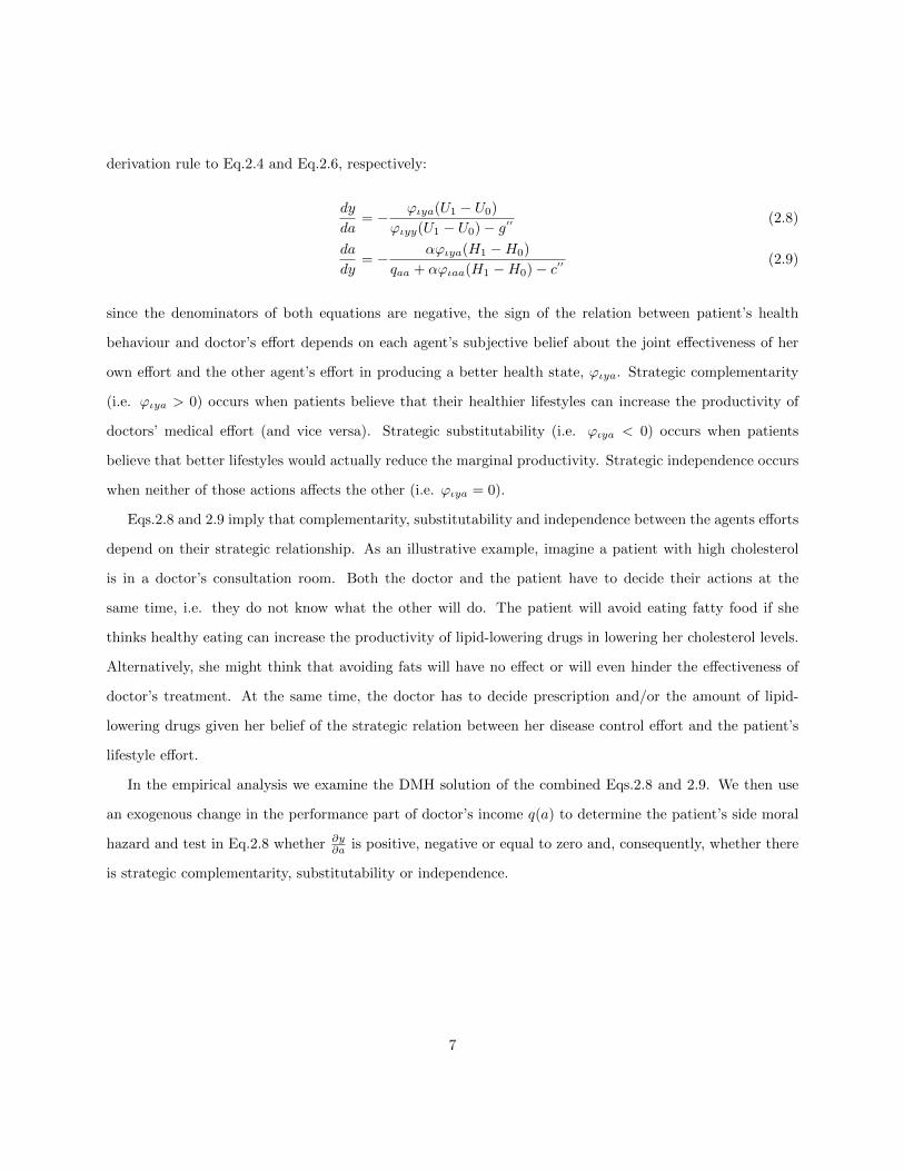
derivation rule to Eq.2.4 and Eq.2.6, respectively:

dy

da= − ϕιya(U1 − U0)

ϕιyy(U1 − U0)− g′′(2.8)

da

dy= − αϕιya(H1 −H0)

qaa + αϕιaa(H1 −H0)− c′′(2.9)

since the denominators of both equations are negative, the sign of the relation between patient’s health

behaviour and doctor’s effort depends on each agent’s subjective belief about the joint effectiveness of her

own effort and the other agent’s effort in producing a better health state, ϕιya. Strategic complementarity

(i.e. ϕιya > 0) occurs when patients believe that their healthier lifestyles can increase the productivity of

doctors’ medical effort (and vice versa). Strategic substitutability (i.e. ϕιya < 0) occurs when patients

believe that better lifestyles would actually reduce the marginal productivity. Strategic independence occurs

when neither of those actions affects the other (i.e. ϕιya = 0).

Eqs.2.8 and 2.9 imply that complementarity, substitutability and independence between the agents efforts

depend on their strategic relationship. As an illustrative example, imagine a patient with high cholesterol

is in a doctor’s consultation room. Both the doctor and the patient have to decide their actions at the

same time, i.e. they do not know what the other will do. The patient will avoid eating fatty food if she

thinks healthy eating can increase the productivity of lipid-lowering drugs in lowering her cholesterol levels.

Alternatively, she might think that avoiding fats will have no effect or will even hinder the effectiveness of

doctor’s treatment. At the same time, the doctor has to decide prescription and/or the amount of lipid-

lowering drugs given her belief of the strategic relation between her disease control effort and the patient’s

lifestyle effort.

In the empirical analysis we examine the DMH solution of the combined Eqs.2.8 and 2.9. We then use

an exogenous change in the performance part of doctor’s income q(a) to determine the patient’s side moral

hazard and test in Eq.2.8 whether ∂y∂a is positive, negative or equal to zero and, consequently, whether there

is strategic complementarity, substitutability or independence.

7

3 Data and Descriptive Statistics

Examining the DMH problem requires data on both patients’ and practices’ behaviours. We therefore

link two data sources to each other: the English Longitudinal Study of Ageing (ELSA) and the National

Health Service Quality Management and Analysis System (QMAS) database. In this section we describe

each data source in turn and provide some simple descriptive statistics of our sample before discussing the

way in which we utilise information on doctors’ payment incentives.

3.1 English Longitudinal Study of Ageing (ELSA)

The English Longitudinal Study of Ageing (ELSA) is a biannual survey and the first study of its kind in

the UK to connect the full range of topics necessary to understand the economic, social, psychological and

health elements of the ageing process. Our analysis uses waves 2 and 3 of ELSA corresponding to the years

2004 and 2006, respectively, because the exogenous change in doctors’ remuneration occurs in this period.

ELSA is designed to be a representative sample of those aged 50 or over and living in private households

in England. For the purpose of our analysis we use data from the “core” ELSA interview questionnaires on

diagnosis of diseases, health behaviours, demographic characteristics, and wealth. ELSA participants were

asked whether they have been diagnosed by a doctor with one of the following conditions: diabetes, high

blood pressure (hypertension), angina, heart attack, heart failure, heart murmur, irregular heart rhythm

and other heart problems. We choose to use this subset of conditions because they correspond to the

target population for the doctors’ performance payments. Participants who confirmed at least one of these

conditions were classified as having CVD. We select individuals who reported CVD in the 2004 wave of

ELSA so that we do not pick up case-finding due to the (reforms to the) payment system. From an initial

sample of over 7,000 individuals in 2004 and over 6,000 in 2006 who can be successfully matched to their

doctors (more details on the matching are described in sub-section 3.2) we obtain a sample of over 3,000

individuals with CVD who are observed both in 2004 and 2006.

We consider a number of socioeconomic characteristics such as household size, and whether the respondent

is married or cohabiting as opposed to being divorced or separated, widowed or never married. We also

consider whether the respondent is employed or self-employed as opposed to unemployed, disabled, looking

after home or family or retired. We use total wealth as the socio-economic variable since it demonstrates a

8

higher correlation with health than income in older populations [see Demakakos et al. (2008)]. Total (non-

pension) wealth is defined as the sum of financial wealth, physical wealth (such as business wealth, land

or jewellery) and housing wealth after deducting debts. This variable is measured in pounds sterling and

deflated by the Consumer Price Index with 2005 as the base year.

As lifestyle behaviours we consider physical activity, smoking and drinking behaviour because they are

available both in 2004 and in 2006. All lifestyle behaviours have been coded to be increasing in health effort

(i.e. the number of cigarettes is coded as negative). We use a measure of physical activity derived from self-

reports and categorised as follows: 1 (none) - not working or sedentary occupation, or engages in only mild

exercise; 2 (low) - working in a job involves standing and/or engaging in moderate activity; 3 (moderate)

- working in a job involving physical work and/or engaging in vigorous activity once a week to 1-3 times a

month; 4 (high) - engaged in heavy manual work and/or doing vigorous leisure activity more than once a

week. In each wave of the survey respondents are asked the number of cigarettes smoked on a weekday or

weekend. We calculate a weighted average of the two to determine the average number of cigarettes smoked

per day. We recode it to be negative in order to indicate a lifestyle behaviour increasing in health effort.

Alcohol consumption is defined as frequency of consumption in the past year. It is categorised as follows:

1=Daily; 2=Frequently: once per week or more; 3=Rarely: once/twice per week or once every two months;

4=Never.

Table 6.1 reports descriptive statistics for 2,500 CVD patients (top panel) and 240 smokers amongst

them (bottom panel). The distribution of physical activity shifts towards higher intensity from 2004 to 2006.

Similarly, the proportion of people drinking either daily or frequently decreases from 2004 to 2006. There is

also a reduction in the average number of cigarettes from 14 in 2004 to about 11 in 2006.

3.2 The Quality Management and Analysis System database

The data on quality of care for over 8,000 family practices in England is stored in the National Health

Service Quality Management and Analysis System (QMAS) database2. We use this database to obtain the

codes and addresses of all practices in England.

As part of the nurse visits carried out in 2004 and 2008 ELSA respondents were asked for the name and

address of their GP. The initial sample of ELSA respondents for whom we had some information on the

2The data is freely available at: http://www.connectingforhealth.nhs.uk/systemsandservices/gpsupport/qmas.

9

practice they were registered with was 7,332 in 2004 and 8,138 in 2008. After a two-stage imputation process,

we have successfully matched to practices about 82% and 80% of wave 2 and 4 initial ELSA respondents.

Of the 9,168 individuals who did not move between waves 2 and 4 we successfully matched about 73% to

practices in wave 3. The majority of these respondents have been uniquely matched to practices. However,

due to incomplete postcode or address information, there were multiple potential matches for about 6% and

5% of respondents in waves 2 and 4 respectively. In this case we use information from all the potential

practices, constructing a sampling weight that equals the share of registered patients (i.e. practice j’s list

size) that respondent ι’s matched practice represents to the total list size of all the correspondent matched

practices. This share is equal to one if respondent ι is uniquely matched to practice j and it is less than one

if she is matched to multiple practices3.

The geographical coverage of ELSA is quite good. ELSA contains at least one person registered with 32%

and 31% of all practices in England in 2004 and 2006, respectively. Practices are grouped geographically

into 151 Primary Care Trusts. ELSA contains at least one person from each of the 151 Primary Care Trusts.

Having linked ELSA respondents to their doctors’ practices we are in a position to bring in information

on the performance of that practice and the behaviours of the doctors within it. General practices in the

UK are a group of one to six doctors responsible for a pool of patients. A substantial component (about

20%) of each doctor’s income depends on the performance of the practice measured by the Quality and

Outcomes Framework (QOF). The budget to finance the programme was set for three years starting from

2004 to be £1.8 billion and increased doctors’ income by 25 percent [NHS Review Body (2008)]. We use

QOF data at the practice level to obtain proxies for doctors’ effort and to measure the exogenous change in

their remuneration.

The QOF was officially introduced on 1st April 2004 with measurement of performance on 1st April 2005

for the previous 12 months. Practices are rewarded on the basis of performance on a number of indicators.

Indicators are measured in three main areas: clinical care, practice organisation and patient experience. The

points determine the amount of money in pounds sterling (£) claimed annually. The revenue the practice

earns varies linearly between lower and upper thresholds of coverage, called “achievement” A ∈ [0, 1]4. No

money is received by the practice if achievement is less than or equal to the lower threshold and the maximum

3Our results are unaffected by the inclusion of multiple matches. More details on the data matching process can be madeavailable to the reader upon request.

4Note that practice achievement rate Aj = Prob(aι > 0) with a indicating the average doctor’s effort to patient ι asdescribed in section 2.

10

revenue is received if the practice is on or above the upper threshold [see for further details Gravelle et al.

(2010); Doran et al. (2011)].

In the first year, 76 clinical indicators measured the quality of specific aspects of care for a set of 10

disease conditions. A total of 33 indicators were available for CVD making up for 40% of the 550 total

points available for clinical care in the first year of the scheme5. We select indicators for which there was a

change in the threshold levels and/or in the number of points from 2004 to 2006 and aggregate them into a

Disease Control indicator. Disease Control indicates whether doctors’ effort maintains cholesterol and blood

pressure under the recommended levels (see Table 6.2).

Practice j’s achievement on indicator i is given by Aji =Nji

Djiwhere Nji is the number of patients for

whom indicator i is achieved. The denominator is the number of patients with the specific disease who are

eligible for the indicator. We calculate the points weighted average achievement rates for disease control

in 2004 and 2006 and we report them in Table 6.3. The points weighted average achievement rates of an

average practice is 76% and 83% in 2004 and 2006, respectively.

Practices are paid per point π achieved (after adjustments to patient-mix) with π̄ indicating the maximum

number of available points [see for example, Gravelle et al. (2010)]. Summing up all indicators in Table 6.2

a total of 50 and 52 points, respectively in 2004 and 2006, are available for Disease Control. As the national

average price per point in 2004 was £76, increasing to £125 in 2005, an average practice could earn up to

£2, 888 in 2004 and up to £5, 395 in 2006 for its effort on controlling CVD.

For our empirical strategy we need some way of codifying the effect of changes in the GP payment

sytem between 2004 and 2006 on GPs incentives to carry out various treatments. In order to do this we

define the “power” of the income incentive to be the difference between what practices would receive if they

continued to provide the same quality in 2006 as they did in 2004 but with the new 2006 thresholds (i.e. the

“counterfactual” income as a proportion of maximum available points) and what they actually received in

5More specifically, 15 indicators were available for Coronary Heart Diseases (CHD) with a maximum of 121 points and 18indicators were available for diabetes with 99 points in total. Note that CVD encompasses both CHD and diabetes.

11

2004. After lettingπtji

π̄ti≡ ptji(Lt, U t;At), it follows that:

pji(L06, U06;A04)− pji(L04, U04;A04) ≡

π04′

ji

π̄06i

−π04ji

π̄04i

=

min

{1,max

{(A04

ji −A06iL)

(A06iU −A06

iL), 0

}}−min

{1,max

{(A04

ji −A04iL)

(A04iU −A04

iL), 0

}}(3.1)

with AtiL and AtiU indicating the lower and upper threshold, respectively. Notice that A04iL < A06

iL and

A04iU < A06

iU that is, thresholds increase between 2004 and 2006. After aggregating i indicators for disease

control we have P tj (Lt, U t) =∑k

i=1 ptji(L

t,Ut;At)πti

π̄t with π̄t =∑ki=1 π

ti . Then the size or power of the incentive

is given by P pj ≡ Pj(L06, U06;A04) − Pj(L

04, U04;A04). The absolute value of this incentive determines

the expected loss as it indicates the proportion of available payment that practice j would lose at 2006

thresholds if it kept performing in 2006 at the same level as it did in 2004. The incentive power reported in

Table 6.3 is on average negative as practices expect to earn less in 2006 than in 2004 if they do not increase

their performance. On average, practices would lose around 5%, and they could lose as much as 39% of the

available payment if, maintaining 2004 performance in 2006 they fall short of 2006’s lower payment threshold.

In order to examine the representativeness of our sample of practices, we compare the practices in ELSA

to the full sample of practices in England. In Table A.1 we report the number of practices in England (left

panel) and those in the ELSA sample (right panel) with an achievement rate below the lower threshold,

between the lower and the upper threshold, and above the upper threshold in 2004 and in 2006. The

proportion of total practices in ELSA that fall in each threshold interval is very similar to that of England.

In Table A.2 we report the points weighted average achievement rates and the power of incentive of the full

sample of English practices. As the mean and minimum values, and the standard deviation of the incentive

power in the last row of Table 6.3 do not differ much from that in Table A.2, our sample of practices in

ELSA adequately represents that of England.

4 Empirical Strategy

We relate three patients’ lifestyle behaviours (intensity of physical activity, rarity of alcohol consumption

and reduction of cigarettes) to a proxy of doctors’ effort (disease control). Whilst models for physical activity

12

and alcohol drinking are run on the full sample, cigarettes consumption is modelled on the sample of smokers

in 2004 as very few individuals started smoking between 2004 and 2006. Lifestyle behaviours are examined

separately because we found a very low correlation between changes in health behaviours between 2004

and 2006. This is not a unique feature of ELSA data as it has been found previously in the Health and

Retirement Study (Cutler and Glaeser (2005)) which contains detailed information on a large representative

sample of individuals aged 50 and over in the United States. We address potential reverse causality between

doctor’s supply of medical treatment and her expectation of patients’ health behaviours in two ways. First,

as practice activities are measured up to 15 months prior to their recording time, they are observed prior to

the reported lifestyle behaviour. Second, we examine practice-level achievement rates rather than individual

treatment.

We consider a linear model for each lifestyle behaviour in 2004 and 2006:

yι(j)t = β0xι(j)t + γ0Aι(j)t + cι(j) + ει(j)t

and we then take the first-difference between 2006 and 2004:

∆yι(j)t = β0∆xι(j)t + γ0∆Aι(j)t + ∆ει(j)t (4.1)

where ∆y indicates the difference in lifestyle behaviours between 2006 and 2004 of individual ι registered

with practice j6. As a result, the individual time-invariant unobserved component cι(j) is differenced out.

Amongst the individual effects we consider the (unobserved) propensity to engage in lifestyle behaviours.

∆Aι(j)t indicates the change in practice j’s points weighted average achievement rates for disease control

between 2004 and 2006 (i.e. the change in the average doctor’s effort). The coefficient γ0 indicates the DMH

solution of the reaction functions’ slopes in Eqs.2.8 and 2.9 and relates to the fact that both the (average)

doctor and the patient choose their actions simultaneously without being able to infer the other agent’s effort

from the realised state of health. For instance, the doctor may increase her effort in managing CVD because

she thinks the patient puts less effort in her lifestyle behaviours; at the same time, the patient might put less

6We account for multiple practices matched to individuals as follows. We create a dataset with 10 random draws of practiceswithin each stratum (i.e. an individual-wave observation) where the probability of drawing is given by the constructed samplingweights. Note that if an ELSA respondent is uniquely matched to a single practice then she will be duplicated 10 times. Thenwe weight the observations in the regression using the constructed sampling weights.

13

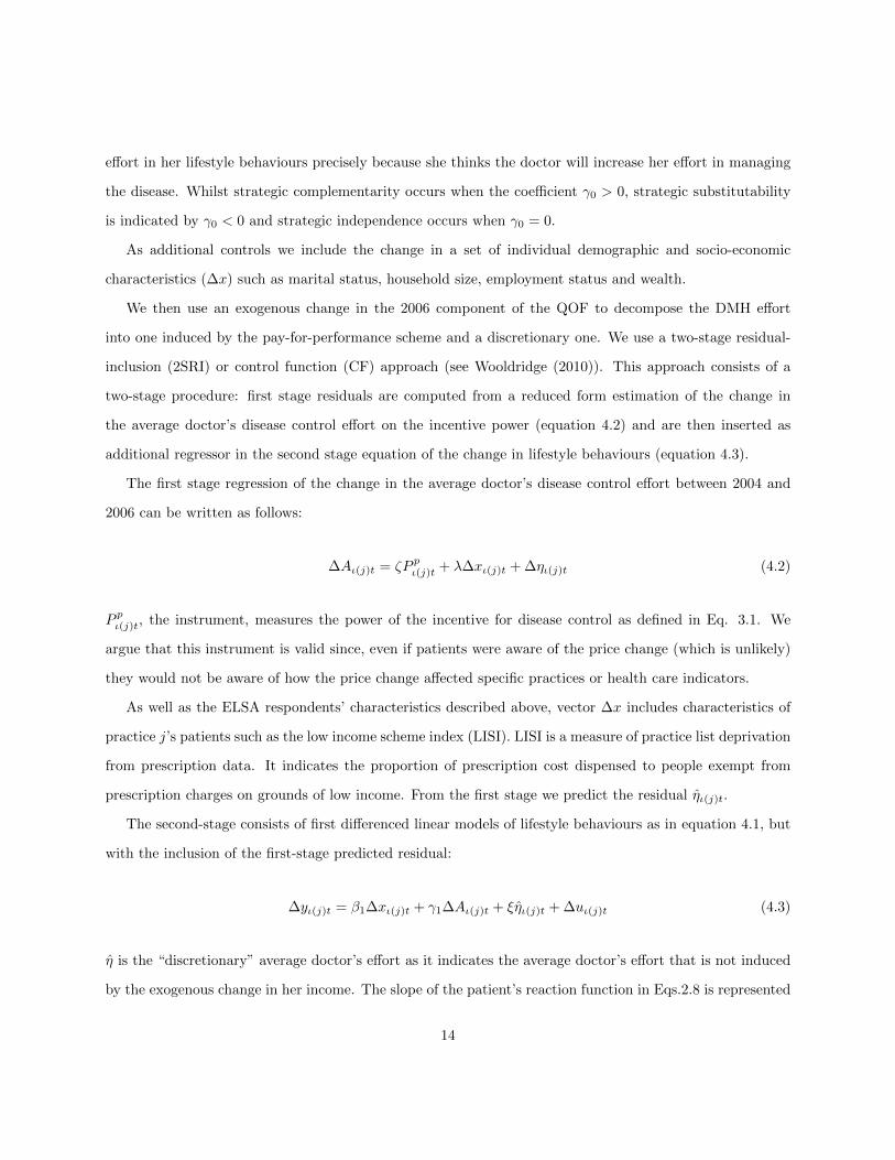
effort in her lifestyle behaviours precisely because she thinks the doctor will increase her effort in managing

the disease. Whilst strategic complementarity occurs when the coefficient γ0 > 0, strategic substitutability

is indicated by γ0 < 0 and strategic independence occurs when γ0 = 0.

As additional controls we include the change in a set of individual demographic and socio-economic

characteristics (∆x) such as marital status, household size, employment status and wealth.

We then use an exogenous change in the 2006 component of the QOF to decompose the DMH effort

into one induced by the pay-for-performance scheme and a discretionary one. We use a two-stage residual-

inclusion (2SRI) or control function (CF) approach (see Wooldridge (2010)). This approach consists of a

two-stage procedure: first stage residuals are computed from a reduced form estimation of the change in

the average doctor’s disease control effort on the incentive power (equation 4.2) and are then inserted as

additional regressor in the second stage equation of the change in lifestyle behaviours (equation 4.3).

The first stage regression of the change in the average doctor’s disease control effort between 2004 and

2006 can be written as follows:

∆Aι(j)t = ζP pι(j)t + λ∆xι(j)t + ∆ηι(j)t (4.2)

P pι(j)t, the instrument, measures the power of the incentive for disease control as defined in Eq. 3.1. We

argue that this instrument is valid since, even if patients were aware of the price change (which is unlikely)

they would not be aware of how the price change affected specific practices or health care indicators.

As well as the ELSA respondents’ characteristics described above, vector ∆x includes characteristics of

practice j’s patients such as the low income scheme index (LISI). LISI is a measure of practice list deprivation

from prescription data. It indicates the proportion of prescription cost dispensed to people exempt from

prescription charges on grounds of low income. From the first stage we predict the residual η̂ι(j)t.

The second-stage consists of first differenced linear models of lifestyle behaviours as in equation 4.1, but

with the inclusion of the first-stage predicted residual:

∆yι(j)t = β1∆xι(j)t + γ1∆Aι(j)t + ξη̂ι(j)t + ∆uι(j)t (4.3)

η̂ is the “discretionary” average doctor’s effort as it indicates the average doctor’s effort that is not induced

by the exogenous change in her income. The slope of the patient’s reaction function in Eqs.2.8 is represented

14

by γ1, the patient-side moral hazard (PMH) coefficient. After including the first stage regression residual,

the change in effort ∆Aι(j)t is one exogenously induced by the payer. As a result, a coefficient γ1 > 0

(γ1 < 0) indicates that the patient complements (substitutes) higher average doctor’s effort with better

(worse) lifestyle behaviours.

All models have been estimated separately for all CVD patients and for those amongst them who were

smoking in 2004.

5 Results

In Table 6.4 we report first differenced models of the change in lifestyle behaviours between 2004 and 2006

regressed on the changes in disease control and other socio-economic characteristics for all CVD patients

(Models I-II) and the smokers amongst them (Model III). The coefficients on disease control indicate the

slope of the reaction functions in Eqs.2.8 and 2.9, that is, the patient’s response to the average doctor and the

average doctor’s response to the patient. We find weak evidence of strategic complementarity in cigarettes

consumption as the average doctor’s effort increases the productivity of the patient’s reduced cigarettes

consumption and, at the same time, the patient’s lower cigarettes consumption increases the productivity of

doctor’s disease control effort. Although this effect is not statistically significant, the point estimates suggest

that a one percentage point increase in disease control would reduce the number of cigarettes per day by

almost 0.1. For an average practice increasing its rate of disease control from 76% to 83% this corresponds

to about 0.7 cigarettes per day per smoker.

We then use the exogenous change in the payment system to decompose the effort level into one induced

by the change in the QOF (i.e. the coefficient γ1 indicating the PMH solution) and a discretionary one (i.e.

the coefficient ξ of the first stage predicted residual)7.

The first-stage regression in Table 6.5 reports the power of incentive to be a strong predictor of changes

in the average doctor’s disease control effort8. A one percentage point increase in the power of the incentive

reduces the average doctor’s effort in disease control by about 0.5 percentage points.

7As a robustness check we have run all the models in this section with a non-linear specification. The results are qualitativelysimilar and are available to the reader on request. We have chosen to display the linear specifications because the interpretationof the coefficients is more straightforward.

8We run a first stage regression on the sample for each lifestyle behaviour.

15

The second-stage regressions of each health behaviour are reported in Table 6.6, for all CVD patients

(Models I-II) and the smokers amongst them (Model III)9.

The results suggest that doctors do not make strategic decisions about their induced efforts as the

relationship between their induced effort and patients’ effort reveals only how patients respond to doctors,

not a combination of how doctors respond to patients and patients respond to doctors. We find that patients

complement a more effective average disease control effort with better lifestyle behaviours. For an average

practice increasing its rate of disease control from 76% to 83% there would be a reduction of the frequency of

alcohol drinking by 0.5 days per patient per month and a reduction in cigarettes consumption by 1.4 per day

per smoker. But the former is only weakly statistically significant. We find that the DMH effort response is

actually lower than the PMH one as γ0 < γ1, although it was not statistically significant in Table 6.4. The

PMH complementary effort in cigarettes consumption is double the magnitude of the DMH one.

We also find that doctors put more effort in effectively controlling CVD of the patients with unhealthier

lifestyles. A one percentage point increase in doctors’ discretionary rate of disease control is associated with

an increase of the frequency of alcohol consumption by 0.01 days per patient per month and the number

of cigarettes per day per smoker by 0.3. The coefficient ξ < 0 indicates that the average doctor uses her

discretionary effort to substitute for her patient’s larger consumption of alcohol and cigarettes.

6 Conclusions

Although it is recognised that health is a joint production process between doctors and patients, the

strategic interaction between these agents is often neglected. From the patient’s point of view, a doctor’s

medical intervention may lower the cost of unhealthy behaviours compensating for their negative effects

through more effective health care. Individuals may therefore reduce their effort in undertaking healthier

lifestyles. Doctors, on the other hand, might also change their effort in response to their patients’ lifestyle

behaviours. Lack of an appropriate conceptual framework and lack of data are two of the reasons for this

gap in research. In this paper we attempt to make a contribution in both areas.

9As the proportion of people who are single or are employed is quite low in this old population, we have also tried a modelwith the levels of marital status and employment and including age and gender. The size of the main coefficient of interest waslarger and even more statistically significant. These results are available to the reader on request.

16

We first conceptualise the patient-doctor interaction in a double-moral hazard framework based on Schnei-

der (2004) where each agent’s effort is hidden from the other party. We show that the relation between

doctors’ and patients’ effort depends on their strategic interaction, that is, whether each agent’s effort in-

creases the productivity of the other party. As patients’ efforts we consider frequency of physical activity,

frequency of alcohol drinking and average number of cigarettes per day. As doctors’ input we consider their

CVD control effort.

We then develop a new data linkage between over 2,000 CVD patients aged 50 and over from the English

Longitudinal Study of Ageing and the GP practices they are registered with between 2004 and 2006. Through

a first-differenced control function regression we find evidence of strategic complementarity, as patients

increase their efforts in healthier lifestyle behaviours when doctors increase their treatment efforts in response

to an exogenous change in their remuneration system. This association is stronger for frequency of alcohol

drinking and cigarettes consumption as they are more observable to the doctor and produce the highest

health benefits to the patient. For an average practice increasing its CVD control rate from 76% to 83%

there is a reduction of frequency of drinking by 0.5 days per patient per month and cigarettes consumption

by 1.4 cigarettes per smoker per day. We also find that the average doctor compensates for her patient’s

unhealthy smoking and drinking by increasing her effort in CVD control.

One of the limitations of this study is the lack of data on individual doctor’s disease control. We use

instead the average performance of the practice. This generates a form of measurement error but on the other

hand avoids a selection bias caused by matching of doctors and patients. A second limitation concerns the

lack of variation in the power of the incentive as instrument for the average doctor’s effort. This instrument

can only pick up exogenous changes in payment that occur between lower and upper thresholds as practices

are not paid anything or they are paid the maximum amount irrespective of how far below or above the

lower and upper thresholds they are. Additionally, the small sample size prevents us from analysing practice

heterogeneities around the lower and upper thresholds. Despite picking up a local average treatment effect,

our results are relevant for all those practices that were not always under or over performing throughout the

sample period (over 80% of the 2006 practices). As in other studies, we do have a fair amount variation in

the first two years which is one of the reasons we have only analysed the first two years of the policy. Finally,

whilst we have attempted to distinguish between double-side and patient’s side moral hazard, the lack of an

appropriate instrument for the patient’s effort prevents us from examining the doctor’s side moral hazard.

17

Our results suggest that neglecting strategic interactions between doctors and patients can lead to under-

estimating the impact of health care reforms on patients’ health behaviours, suggesting that payers should

take these interactions into account when designing policies that change doctor’s intervention. In addition,

our analysis demonstrates the potential value of research exploiting matched data on doctors and their pa-

tients. Such data are becoming more readily available for researchers both in the UK elsewhere, and we

would expect this development to lead to further important empirical insights on health behaviours and their

interaction with healthcare.

Future research should examine how repeated interactions and treatment intensities can affect these

double-side asymmetries between doctors and patients. It will be interesting to examine the marginal pro-

ductivity of lifestyle behaviours, the impact of DMH on long-term outcomes and spillovers between primary

and secondary care resulting from information asymmetries.

18

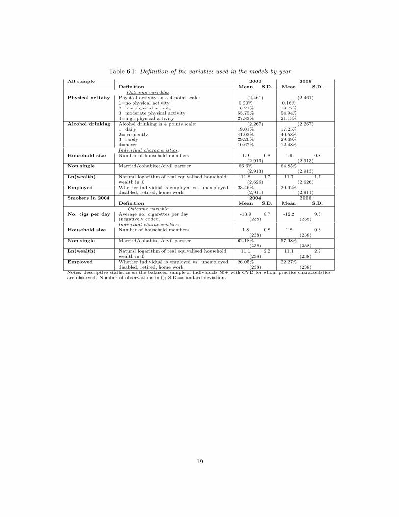
Table 6.1: Definition of the variables used in the models by year

All sample 2004 2006Definition Mean S.D. Mean S.D.

Outcome variables:Physical activity Physical activity on a 4-point scale: (2,461) (2,461)

1=no physical activity 0.20% 0.16%2=low physical activity 16.21% 18.77%3=moderate physical activity 55.75% 54.94%4=high physical activity 27.83% 21.13%

Alcohol drinking Alcohol drinking in 4 points scale: (2,267) (2,267)1=daily 19.01% 17.25%2=frequently 41.02% 40.58%3=rarely 29.20% 29.69%4=never 10.67% 12.48%Individual characteristics:

Household size Number of household members 1.9 0.8 1.9 0.8(2,913) (2,913)

Non single Married/cohabitee/civil partner 66.6% 64.85%(2,913) (2,913)

Ln(wealth) Natural logarithm of real equivalised household 11.8 1.7 11.7 1.7wealth in £ (2,626) (2,626)

Employed Whether individual is employed vs. unemployed, 23.46% 20.92%disabled, retired, home work (2,911) (2,911)

Smokers in 2004 2004 2006Definition Mean S.D. Mean S.D.

Outcome variable:No. cigs per day Average no. cigarettes per day -13.9 8.7 -12.2 9.3

(negatively coded) (238) (238)Individual characteristics:

Household size Number of household members 1.8 0.8 1.8 0.8(238) (238)

Non single Married/cohabitee/civil partner 62.18% 57.98%(238) (238)

Ln(wealth) Natural logarithm of real equivalised household 11.1 2.2 11.1 2.2wealth in £ (238) (238)

Employed Whether individual is employed vs. unemployed, 26.05% 22.27%disabled, retired, home work (238) (238)

Notes: descriptive statistics on the balanced sample of individuals 50+ with CVD for whom practice characteristicsare observed. Number of observations in (); S.D.=standard deviation.

19

Table 6.2: Description of indicators of doctors’ disease control

Indicator Description 2004 2006name LT UT Points LT UT Points

The percentage of patients withCHD8 coronary heart disease whose last 25 60 16 40 70 17

measures cholesterol (measured inthe last 15 months is 7mmol/l or less).The percentage of patients with diabetes

DM7 in whom the last HbA1C is 10 or less (or 25 85 11 40 90 11equivalent test/reference range depen-ding on local laboratory) in last 15 months.

DM12 The percentage of patients with diabetes 25 55 17 40 60 18in whom the last blood pressure is 145/85or less.

DM17 The percentage of patients with diabetes 25 60 6 40 70 6whose last measured total cholesterolwithin previous 15 months is 5 or less.

LT=Lower Threshold; UT=Upper Threshold.

Table 6.3: Summary statistics on the average achievement rates and power of incentive

Mean Min. Max. Std. Dev.

Disease Control in 2004 [Pj(L04, U04;A04)] 0.76 (2,644) 0.004 1 0.08

Disease Control in 2006 [Pj(L06, U06;A06)] 0.83 (2,523) 0.08 1 0.05Power of incentive [Pp

j ] -0.05 (2,096) -0.39 0 0.07

Note: Statistics weighted by the constructed sampling weights. The achievement rates are weighted by the number ofpoints. Sample sizes in () represent practices.

Table 6.4: Coefficients of first differenced linear models of health behaviours

Model I: Model II: Model III:∆Physical activity ∆Alcohol drinking ∆No. cigarettes

∆Disease Control (γ0) 0.29 -0.10 8.41(0.24) (0.23) (7.25)

∆Non single 0.01 0.12 1.88(0.11) (0.10) (1.81)

∆Employed 0.02 0.08* 1.31(0.06) (0.04) (2.04)

∆Household size -0.01 0.04 -1.06(0.03) (0.03) (0.93)

∆Ln(equivalised wealth) 0.02 0.02 -0.16(0.02) (0.02) (0.57)

Constant -0.07*** 0.07*** 1.10(0.02) (0.02) (0.75)

No. observations 22,498 20,810 2,378No. individuals 2,251 2,082 238No. practices 1,512 1,401 247Statistics weighted by the constructed sampling weights and clustered std. errors in (). No. observations for the 10 imputeddatasets on the sample of people aged 50+ with CVD. Model III on sample of smokers in 2004. Lifestyles increasing in healtheffort: intensity of physical activity, rarity of alcohol drinking and reduction in no. cigarettes.∗p < 0.1,∗∗ p < 0.05,∗∗∗ p < 0.01.

20

Table 6.5: First stage coefficients of first differenced linear models of practice achievement on the power ofthe incentive

∆Disease Control ∆Disease Control ∆Disease Controlon physical activity sample on alcohol sample on no. cigarettes sample

Power of Incentive -0.52*** -0.51*** -0.55***(0.03) (0.03) (0.04)

∆Non single 0.0004 -0.004 -0.001(0.01) (0.01) (0.02)

∆Employed -0.01 -0.01 0.003(0.004) (0.005) (0.01)

∆Household size 0.0004 0.001 -0.001(0.002) (0.003) (0.01)

∆Ln(equivalised wealth) 0.001 0.0003 0.0001(0.002) (0.002) (0.004)

∆LISI -0.003* -0.002* -0.001(0.001) (0.001) (0.001)

Constant 0.05*** 0.05*** 0.05***(0.002) (0.002) (0.004)

No. observations 22,467 20,785 2,378No. individuals 2,249 2,080 238No. practices 1,508 1,398 247Statistics weighted by the constructed sampling weights and clustered std. errors in (). No. observations for the 10 imputeddatasets on the sample of people aged 50+ with CVD. Model III on sample of smokers in 2004.∗p < 0.1,∗∗ p < 0.05,∗∗∗ p < 0.01.

Table 6.6: Second stage coefficients of first differenced linear models of health behaviours

Model I: Model II: Model III:∆Physical activity ∆Alcohol drinking ∆No. cigarettes

∆Disease Control (γ1) 0.14 0.68* 23.62**(0.38) (0.39) (9.96)

Disease Control residuals (ξ) 0.22 -1.13** -29.44**(0.47) (0.46) (11.66)

∆Non single 0.01 0.12** 2.02(0.11) (0.10) (1.66)

∆Employed 0.02 0.08* 1.22(0.06) (0.04) (1.99)

∆Household size -0.01 0.04 -1.07(0.03) (0.03) (0.81)

∆Ln(equivalised wealth) 0.02 0.02 -0.15(0.02) (0.02) (0.57)

Constant -0.05* 0.01 -0.13(0.03) (0.03) (0.92)

No. observations 22,467 20,785 2,378No. individuals 2,249 2,080 238No. practices 1,508 1,398 247Statistics weighted by the constructed sampling weights and clustered std. errors in (). No. observations for the 10 imputeddatasets on the sample of people aged 50+ with CVD. Model III on sample of smokers in 2004. Lifestyles increasing in healtheffort: intensity of physical activity, rarity of alcohol drinking and reduction in no. cigarettes.∗p < 0.1,∗∗ p < 0.05,∗∗∗ p < 0.01.

21

A Comparisons between practices in England and ELSA

Table A.1: Sample of practices in England and ELSA by threshold levels for Disease Control

England: ELSA/Practice linkageLT (LT, UT) UT Total LT (LT, UT) UT Total

2004/05 3 2,675 5,609 8,287 1 665.90 1,979.06 2,645.96(0.04%) (32.28%) (67.68%) (0.04%) (25.17%) (74.80%)

2006/07 1 2,077 6,279 8,357 0 428.70 2,094.23 2,522.93(0.01%) (24.85%) (75.13%) (0.00%) (16.99%) (83.01%)

Note: Statistics weighted by the constructed sampling weights LT=Upper Threshold level and UT=LowerThreshold level; (LT, UT) between lower and upper threshold. Achievements from ELSA practices are calculatedon the sample of individuals 50+. Proportion of total sample in ().

Table A.2: Summary statistics on the points weighted average achievement rates and power of incentive(England)

Mean Min. Max. Std. Dev.

Disease Control [Pj(L04, U04;A04)] 0.76 (8,287) 0.004 1 0.09

Disease Control [Pj(L06, U06;A06)] 0.83 (8,357) 0.08 1 0.06Power of incentive [Pp

j ] -0.06 (8,055) -0.40 0 0.08

Note: Statistics weighted by the constructed sampling weights. Sample sizes in () represent practices.

22

References

Agrawal P. Double moral hazard, monitoring and the nature of contracts. Journal of Economics, 2002; 75(1):

33-61.

Arrow K. Uncertainty and the welfare economics of medical care. American Economic Review, 1963; 53:

941-973.

Cooper R. and Ross T.W. Product warranties and double moral hazard. The RAND Journal of Economics

1985; 16(1): 103-113.

Cutler D.M. and Glaeser E. What Explains Differences in Smoking, Drinking, and Other Health-Related

Behaviors? The American Economic Review; 95(2): 238-242.

Demakakos P., Nazroo J., Breeze E., Marmot M. Socioeconomic status and health. The role of subjective

social status. Social Science and Medicine 2008; 67: 330-340.

Dybvig P.H. and Lutz N.A. Warranties, durability, and maintenance: two-sided moral hazard in a continuous-

time model. The Review of Economic Studies, 1993; 60: 575-597.

Doran T., Kontopantelis E., Valderas J.M., Campbell S., Roland M., Salisbury C. and Reeves D. Effect of

financial incentives on incentivised and non-incentivised clinical activities: longitudinal analysis of data

from the UK Quality and Outcomes Framework. BMJ 2011; 342:1-12.

Emons W. Warranties, moral hazard and the lemons problems. Journal of Economic Theory, 1989; 46: 16-33.

Eswaran M. and Kotwal A. A theory of contractual structure in agriculture. American Economic Review,

1985; 75(3): 352-367.

Evans R.G. Supplier-induced demand: some empirical evidence and implications. In M. Perlman (Ed.), The

economics of health and medical care, 1974: 162-173. new York: Stockton press.

Fichera E. and Sutton M. State and self investments in health. Journal of Health Economics 2011; 30(6):

1164-1173.

Gravelle H., Sutton M. and Ma A. Doctor behaviour under a pay for performance contract: treating, cheating

and case finding? The Economic Journal, 2010; 120(February) F129-156.

23

NHS Review Body Twenty-Third Report, 2008. Ref: ISBN 9780101733724.

Parsons D.O. Double-sided moral hazard in job displacement insurance contracts. IZA Discussion Paper

Series, 2011 DP No. 6003.

Pauly M.V. The economics of moral hazard: Comment. American Economic Review, 1968; 58: 531-537.

Prendergast C. The role of promotion in inducing specific human capital acquisition. Quarterly Journal of

Economics, 1993; 108(2): 523-534.

Prendergast C. The provision of incentives in firms. Journal of Economic Literature, 1999; 37: 7-63.

Reid J.D. Jr. The theory of share tenancy revisited-again. Journal of Political Economy, 1977; 85(2): 403-407.

Richard S. Information Problems in the market for medical services. In Arnold Picot and Schlicht, Ekkehart

(eds.), Firms, markets, and contracts: contributions to neoinstitutional economics. Heidelberg: Physica,

1996; 200-219.

Schneider U. Asymmetric Information and the Demand for Health Care: the Case of Double Moral Hazard.

Journal of Applied Social Science Studies 2004; 124(2): 233-256.

Schneider U. and Ulrich V. The physician-patient relationship revisited: the patient’s view. Int J Health

Care Finance Econ, 2008; 8: 279-300.

Wooldridge J.M. Econometric Analysis of Cross Section and Panel Data, MIT Press, 2nd edition; 2010.

24