RICE UNIVERSITY

By

A THESIS SUBMITTED IN PARTIAL FULFILLMENT OF THE REQUIREMENTS FOR THE DEGREE

APPROVED, THESIS COMMITTEE

HOUSTON, TEXAS

Eugene Ng

Doctor of Philosophy

Ang Chen

Peter Varman

Yuhan Peng

April 2020

T. S. Eugene Ng (Apr 15, 2020)T. S. Eugene Ng

Ang Chen (Apr 16, 2020)Ang Chen

ABSTRACT

Enabling QoS Controls in Modern Distributed Storage Platforms

by

Yuhan Peng

Distributed storage systems provide a scalable approach for hosting multiple

clients on a consolidated storage platform. The use of shared infrastructure can lower

costs but exacerbates the problem of fairly allocating the IO resources. Providing per-

formance Quality-of-Service (QoS) guarantees in a distributed storage environment

poses unique challenges. Workload demands of clients shift unpredictably between

servers as their locality and IO intensities fluctuate. This complicates the problem of

providing QoS controls like reservations and limits that are based on aggregate client

service, as well as providing differentiated tail latency guarantees to the clients.

In this thesis, we present novel approaches for providing bandwidth allocation

and response time QoS in distributed storage platforms. For bandwidth allocation

QoS, we develop a token-based scheduling framework to guarantee the maximum and

minimum aggregate throughput of different clients. We introduce a novel algorithm

called pTrans for solving the token allocation problem. pTrans is provably optimal and

has better theoretical and empirical scalability than competing approaches based on

linear-programming or max-flow formulations. For the response time QoS, we intro-

duce Fair-EDF, a framework that extends the earliest deadline first (EDF) scheduler

to provide fairness control while supporting latency guarantees.

iii

Acknowledgments

Firstly, I would like to thank my advisor, Professor Peter Varman, for advising my

PhD research. He provided me excellent guidance in developing research ideas and

conducting research in the field of distributed storage systems and QoS. Professor

Varman also offered a lot of help in publishing the research papers based on the

thesis, as well as in revising this thesis document. I also express my appreciation to

Professor Eugene Ng and Professor Ang Chen for serving on my PhD thesis committee

and providing valuable feedback before and during my PhD defense.

In addition, I thank my teammate, Qingyue Liu, for help in performing the exper-

iments, and in providing useful feedback for paper revisions. I also thank my 4-year

roommate, Peng Du, as well as other friends, for offering me a warm and harmonious

life environment to conduct my PhD research.

Finally, I would like to thank my parents and other family members for their

support and love. Without them, I could not imagine how could I achieve the accom-

plishments in my research.

Contents

Abstract ii

List of Illustrations viii

List of Tables xi

1 Introduction and Overview 1

1.1 Introduction . . . . . . . . . . . . . . . . . . . . . . . . . . . . . . . . 1

1.2 Distributed Storage Platform Overview . . . . . . . . . . . . . . . . . 3

1.2.1 Clustered Storage Systems . . . . . . . . . . . . . . . . . . . . 3

1.2.2 Chip-level Distributed Storage Devices . . . . . . . . . . . . . 4

1.3 QoS Overview . . . . . . . . . . . . . . . . . . . . . . . . . . . . . . . 6

1.3.1 Bandwidth QoS . . . . . . . . . . . . . . . . . . . . . . . . . . 6

1.3.2 Response Time QoS . . . . . . . . . . . . . . . . . . . . . . . 7

1.4 Motivation . . . . . . . . . . . . . . . . . . . . . . . . . . . . . . . . . 8

1.5 Thesis Statement . . . . . . . . . . . . . . . . . . . . . . . . . . . . . 10

1.6 Contributions . . . . . . . . . . . . . . . . . . . . . . . . . . . . . . . 10

1.7 Thesis Organization . . . . . . . . . . . . . . . . . . . . . . . . . . . . 11

2 Bandwidth Allocation QoS 12

2.1 Chapter Overview . . . . . . . . . . . . . . . . . . . . . . . . . . . . . 12

2.2 Problem Statement . . . . . . . . . . . . . . . . . . . . . . . . . . . . 12

2.2.1 Challenges for Distributed Bandwidth Allocation . . . . . . . 15

2.3 bQueue Framework . . . . . . . . . . . . . . . . . . . . . . . . . . . . 18

2.3.1 QoS Model . . . . . . . . . . . . . . . . . . . . . . . . . . . . 18

2.3.2 Token Controller . . . . . . . . . . . . . . . . . . . . . . . . . 21

v

2.3.2.1 Specifications for Token Allocation . . . . . . . . . . 21

2.3.2.2 Two Phase Token Allocation Approach . . . . . . . . 23

2.3.2.3 Demand and Capacity Estimation . . . . . . . . . . 24

2.3.3 Token Scheduler . . . . . . . . . . . . . . . . . . . . . . . . . . 26

2.4 Case Study . . . . . . . . . . . . . . . . . . . . . . . . . . . . . . . . 28

2.5 Chapter Summary . . . . . . . . . . . . . . . . . . . . . . . . . . . . 29

3 Token Allocation 31

3.1 Chapter Overview . . . . . . . . . . . . . . . . . . . . . . . . . . . . . 31

3.2 Problem Description . . . . . . . . . . . . . . . . . . . . . . . . . . . 31

3.3 Direct Problem Formulations . . . . . . . . . . . . . . . . . . . . . . 34

3.3.1 Integer Linear Programming Approach . . . . . . . . . . . . . 34

3.3.2 Max-flow Approach . . . . . . . . . . . . . . . . . . . . . . . . 36

3.4 pTrans Algorithm . . . . . . . . . . . . . . . . . . . . . . . . . . . . . 37

3.4.1 pTrans Algorithm Overview . . . . . . . . . . . . . . . . . . . 39

3.4.2 Prudent Transfer Graph . . . . . . . . . . . . . . . . . . . . . 40

3.4.3 Prudent Token Transfer . . . . . . . . . . . . . . . . . . . . . 43

3.4.4 Performance Optimizations . . . . . . . . . . . . . . . . . . . 46

3.4.4.1 Parallelizing pTrans . . . . . . . . . . . . . . . . . . 46

3.4.4.2 Approximation Approach . . . . . . . . . . . . . . . 47

3.4.5 Comparing pTrans with Preliminary Approaches . . . . . . . . 48

3.5 Chapter Summary . . . . . . . . . . . . . . . . . . . . . . . . . . . . 48

4 Analysis of pTrans Algorithm 50

4.1 Fundamental pTrans Optimality Theorem . . . . . . . . . . . . . . . 50

4.2 Correctness of pTrans . . . . . . . . . . . . . . . . . . . . . . . . . . . 56

4.3 Polynomial Bound of pTrans . . . . . . . . . . . . . . . . . . . . . . . 58

4.4 Comparing pTrans with Edmonds–Karp Algorithm . . . . . . . . . . 66

vi

5 Evaluation of Bandwidth Allocation QoS 67

5.1 Experimental Setup . . . . . . . . . . . . . . . . . . . . . . . . . . . . 67

5.2 QoS Evaluation . . . . . . . . . . . . . . . . . . . . . . . . . . . . . . 69

5.2.1 Bandwidth Allocation at Large Scale . . . . . . . . . . . . . . 69

5.2.2 Effect of Different Parameters . . . . . . . . . . . . . . . . . . 72

5.3 Parallelization Evaluation . . . . . . . . . . . . . . . . . . . . . . . . 74

5.3.1 Comparing pTrans with the LP and Max-flow Approaches . . 76

5.4 Approximation Evaluation . . . . . . . . . . . . . . . . . . . . . . . . 77

5.5 Handling Demand Fluctuation . . . . . . . . . . . . . . . . . . . . . . 79

5.6 Linux Evaluation . . . . . . . . . . . . . . . . . . . . . . . . . . . . . 83

5.6.1 Memcached Evaluation with Static Demand . . . . . . . . . . 83

5.6.2 Memcached Evaluation with Dynamic Demand . . . . . . . . . 84

5.6.3 File I/O Evaluation . . . . . . . . . . . . . . . . . . . . . . . . 87

6 Response Time QoS 90

6.1 Chapter Overview . . . . . . . . . . . . . . . . . . . . . . . . . . . . . 90

6.2 Problem Statement . . . . . . . . . . . . . . . . . . . . . . . . . . . . 90

6.3 Basic Fair-EDF Framework . . . . . . . . . . . . . . . . . . . . . . . 92

6.4 Fair-EDF Controller . . . . . . . . . . . . . . . . . . . . . . . . . . . 93

6.4.1 Occupancy Chart . . . . . . . . . . . . . . . . . . . . . . . . . 93

6.4.2 Handling New Requests . . . . . . . . . . . . . . . . . . . . . 96

6.4.3 Candidate Set Identification . . . . . . . . . . . . . . . . . . . 98

6.5 Fair-EDF Scheduler for Best-Effort Scheduling . . . . . . . . . . . . . 101

6.6 Chapter Summary . . . . . . . . . . . . . . . . . . . . . . . . . . . . 103

7 Evaluation of Response Time QoS 105

7.1 Experimental Setup . . . . . . . . . . . . . . . . . . . . . . . . . . . . 105

7.2 Linux Evaluation . . . . . . . . . . . . . . . . . . . . . . . . . . . . . 106

7.2.1 QoS Evaluation . . . . . . . . . . . . . . . . . . . . . . . . . . 106

vii

7.2.2 Effect of Overestimated Service Time . . . . . . . . . . . . . . 107

7.2.3 QoS Result for More Clients . . . . . . . . . . . . . . . . . . . 109

8 Conclusions and Open Problems 112

8.1 Conclusions . . . . . . . . . . . . . . . . . . . . . . . . . . . . . . . . 112

8.2 Open Problems . . . . . . . . . . . . . . . . . . . . . . . . . . . . . . 113

8.2.1 Bandwidth Allocation QoS . . . . . . . . . . . . . . . . . . . . 113

8.2.2 Response Time QoS . . . . . . . . . . . . . . . . . . . . . . . 114

Bibliography 116

Illustrations

2.1 An illustration of the distributed storage system for the bandwidth

allocation QoS in Example 2.2.1. . . . . . . . . . . . . . . . . . . . . 14

2.2 An illustration of the distributed storage system for the bandwidth

allocation QoS for buckets in Example 2.2.2. . . . . . . . . . . . . . . 15

2.3 The model extending existing fine-grained approaches to support

bandwidth allocation QoS in our distributed model. Comparing to

the framework shown in Figure 2.1, it requires gateway nodes to

collect all the requests of a client and compute the metadata needed

by the scheduler to control the QoS. . . . . . . . . . . . . . . . . . . . 17

2.4 bQueue system hierarchy in Example 2.3.1. . . . . . . . . . . . . . . . 19

2.5 The illustration of coarse-grained bandwidth allocation QoS in

Example 2.3.2. . . . . . . . . . . . . . . . . . . . . . . . . . . . . . . 20

2.6 The illustration of linear extrapolation approach for demand and

capacity estimation. . . . . . . . . . . . . . . . . . . . . . . . . . . . . 26

2.7 Illustration of Example 2.4.1. . . . . . . . . . . . . . . . . . . . . . . 29

3.1 Token allocation determined by max-flow approach for Example 3.3.2. 38

3.2 Illustration of prudent transfer graph in Example 3.4.3. . . . . . . . . 43

3.3 Illustration of transfer path. . . . . . . . . . . . . . . . . . . . . . . . 44

ix

4.1 Illustration of base cases in the proof of Theorem 8. The green edges

indicate the prudent transfer made, and the dotted edge indicates the

new edge j, k generated after making the transfer. . . . . . . . . . . 56

4.2 Illustration the proof of Theorem 9. The green edges indicates the

prudent transfer made, and the dotted edge indicates the new edge

j, k. . . . . . . . . . . . . . . . . . . . . . . . . . . . . . . . . . . . 59

5.1 The specifications of the simulator-based QoS evaluation:

reservations and demand change times for a sample of the clients.

The figures show the results for every 50th client. . . . . . . . . . . . 71

5.2 The number of requests completed for each client in the 5

redistribution intervals. Each client is active (having non-zero

demand) on a set of 8 servers. The figures show the results for every

50th client. . . . . . . . . . . . . . . . . . . . . . . . . . . . . . . . . . 72

5.3 The average error of pTrans with different number of demand changes

and different number of active servers of each client. . . . . . . . . . . 74

5.4 Execution time of pTrans with parallel threads. . . . . . . . . . . . . 75

5.5 The execution time of linear programming for uniform and Zipf

distribution (s = 0.5), with 100 to 1000 clients, 16 servers, r = 1.0

and m = 1.1. In comparison, even single-threaded pTrans can finish

execution for such scale within 0.05 seconds. . . . . . . . . . . . . . . 76

5.6 The controller execution time of pTrans comparing against max-flow,

with 100 to 1000 clients, 64 servers, r = 1.0 and m = 1.1. . . . . . . . 77

5.7 Error and execution time with approximation. . . . . . . . . . . . . . 78

5.8 The token allocation constraints in the demand fluctuation

experiment, with redistribution interval = 100ms. . . . . . . . . . . . 80

5.9 Number of Requests vs Time with Demand Fluctuation. . . . . . . . 82

x

5.10 The number of requests done for pTrans and simple round robin

schedulers. . . . . . . . . . . . . . . . . . . . . . . . . . . . . . . . . . 85

5.11 The number of requests being completed with pTrans scheduler with

reservations and limits. . . . . . . . . . . . . . . . . . . . . . . . . . . 86

5.12 Total number of request completed for pTrans and simple

round-robin scheduler. . . . . . . . . . . . . . . . . . . . . . . . . . . 87

5.13 The Zipf distribution of clients’ reservation requirements in Linux

QoS evaluation. . . . . . . . . . . . . . . . . . . . . . . . . . . . . . . 88

5.14 The the number of requests being completed in Linux QoS evaluation. 89

6.1 The basic Fair-EDF framework. . . . . . . . . . . . . . . . . . . . . . 93

6.2 An illustration of the occupancy chart in

Examples 6.4.1, 6.4.2, 6.4.3, 6.4.4 and 6.4.5. . . . . . . . . . . . . . . 95

6.3 The Fair-EDF framework with best-effort scheduling. . . . . . . . . . 102

7.1 The success ratio of both clients using three policies. . . . . . . . . . 107

7.2 The average response time for both clients using three policies. . . . . 108

7.3 Evaluation result for different overestimated service times. . . . . . . 109

7.4 Evaluation result for the experiment with ten-clients and two-groups. 110

Tables

3.1 Configuration of Example 3.2.1, 3.3.1, 3.3.2 and 3.4.1. Servers 1 and

2 have capacity 100 each. The red and blue clients have reservation of

100 each. di and ai are demand and token allocation on server i. . . . 34

3.2 Configuration of Example 3.4.2. All servers have capacity 100 and all

clients have reservation of 100. di and ai are the demand and token

allocation for server i. . . . . . . . . . . . . . . . . . . . . . . . . . . 41

3.3 Prudent transfer graph for configuration of Table 3.2. Each entry is

PTj,k vector / PTSj,k from server j (row) to server k (column). . . . 43

7.1 The arrival pattern and deadline specifications of the clients. . . . . . 110

1

Chapter 1

Introduction and Overview

1.1 Introduction

Distributed storage systems are widely deployed in today’s datacenters, to scalably

manage the ever-increasing volume of persistent data. Providing Quality of Ser-

vice (QoS) performance guarantees to clients sharing system resources in an impor-

tant requirement of such systems. Performance QoS involves two aspects: resource

allocation that sets policies and mechanisms to divvy up system resources among

competing clients, and request scheduling to enforce the allocation. In general, QoS

guarantees can be for physical resources like network bandwidth and CPU time, or

derived metrics like request throughput and response time. In this thesis, the I/O

request throughput (number of I/O requests per second or IOPS) and tail-latency

guarantees (percentage of requests meeting a specified response time target) will be

used as the QoS measures.

The thesis is motivated by the need to provide bucket QoS in distributed storage

systems, an important requirement that has not been addressed by existing works.

A bucket is a collection of related stored objects that are treated as a single logical

entity for purposes of QoS. In practice, a bucket will consist of several directories,

program or data files, or file chunks, belonging to a designated owner. The bucket

objects may be accessed by multiple clients authorized by the owner. For instance,

the bucket owner may be a department within an organization, and the clients could

2

be departmental team members. The owner of the bucket is responsible for paying

for the storage services for the bucket objects by the different authorized clients. A

bucket can be distributed across multiple storage nodes based on the data allocation

policies of the storage system.

Although many existing QoS studies have been proposed over the past two decades,

most approaches focused on providing QoS in a centralized server environment rather

than a distributed server cluster. A few approaches to QoS for distributed systems

that have been proposed, impose strong restrictions that make them unsuitable for

providing bucket QoS (see Section 1.3.1).

Providing bucket QoS in a distributed environment is challenging, because of

the spatial and temporal variability in demand and capacity distributions across the

servers. Firstly, since a bucket’s objects are distributed by the storage system across

multiple servers, the aggregate bucket demand can be distributed unevenly on dif-

ferent servers. In addition, the rate at which a server can perform I/Os (referred to

as the server capacity), may also depend on the workload characteristics. Finally,

requests for multiple buckets may overload some servers, raising the questions of

which requests to serve, which to defer, and which to drop, in order to meet QoS

requirements.

In this thesis, we introduce novel QoS algorithms for the QoS support in dis-

tributed storage platforms. We focus on bandwidth allocation QoS and response

time QoS. For bandwidth QoS, we focus on providing reservations and limits, which

represent the minimum and maximum I/Os per second allowed for the bucket. We

present bQueue, a token-based framework for bandwidth QoS, and pTrans, a scal-

able algorithm for dynamic token distribution. For response time QoS, we focus on

meeting the tail-latency requirements of the buckets, in which each bucket specifies

3

the percentage of requests that must meet a specified latency bound. We introduce

Fair-EDF, which provides support for differentiated latency guarantees. The pro-

posed algorithms can be applied for both conventional client QoS and bucket QoS ∗.

We also present empirical evaluation results of the proposed QoS algorithms, and

show that they provide reliable QoS support.

1.2 Distributed Storage Platform Overview

1.2.1 Clustered Storage Systems

Clustered storage systems such as Ceph [1], GlusterFS [2], Amazon’s Cloud Stor-

age [3], FAB [4], Kudu [5], Dynamo [6], Cassandra [7], HDFS [8], vSAN [9] and

VMWare storage DRS [10], provide a scalable and economical approach for the stor-

age of huge data sets over multiple storage servers. When deployed in a datacenter

these systems are shared among multiple clients, each representing tens to hundreds

of users. Clients require predictable performance typically codified in service-level

objectives (SLOs) such as guaranteed throughput (averaged over a specified duration)

or a maximum response time for a specified percentage of its requests.

Object-based storage decouples namespace management from the underlying hard-

ware, facilitating the use of decentralized scale-out architectures spread over multiple

storage servers (even geographical regions), and supports APIs for remote access to

stored data. Multiple related objects can be encapsulated within logical containers

called buckets and accessed using object identifiers. Amazon S3, for instance, treats

buckets and objects as controllable resources and provides APIs to create or delete

buckets and upload objects. The storage system is responsible for storage and access

∗To maintain generality, we use the term client as the entity for the QoS support. When providingbucket QoS, clients refer to the owners of the buckets.

4

of objects. Objects may be sharded for manageability, and distributed over multiple

storage nodes for fault tolerance and performance, while decentralized protocols pro-

vide concurrency control and manage object consistency. A cluster manager monitors

the performance of nodes and links and is responsible for recovery from failures.

The focus of this thesis is on sharing the storage subsystem. In this scenario,

the storage server must provide explicit controls for service differentiation to prevent

some clients from unfairly monopolizing system resources, and favoring preferred

customers with better service when there is resource contention. In addition, service

differentiation is also necessary to prioritize system usage over client needs. For

instance, I/O traffic to rebuild a failed node on a replacement server competes with

normal application traffic; QoS policies must permit rebuilding to proceed quickly

while avoiding unreasonable application slowdowns.

1.2.2 Chip-level Distributed Storage Devices

A new generation of non-volatile memory devices and interfaces are changing the

traditional storage landscape made up of SSA/SATA based hard disks (HDs) and

solid-state devices (SSDs). The adoption of the NVMe interface, a purpose-crafted

protocol to access SSDs using the PCIe bus standard, has increased the performance

of modern SSDs by orders of magnitude, while new memory-bus connected persistent

memory devices like Optane DC promise to further blur the performance gap between

volatile DRAM memory and non-volatile storage. NVMe over Fabric protocols based

on Remote Direct Memory Access (RDMA) and Fiber Channel (FC) technologies

are poised to bring the latency and parallelism advantages of NVMe to distributed

storage. These hardware innovations have raised questions about how to structure

storage system software to exploit their unique characteristics and handle newly-

5

exposed performance bottlenecks.

Datacenter storage is a shared resource that is accessed by hundreds or thousands

of concurrent users. Performance isolation techniques are usually deployed at the OS

layer to allocate I/O bandwidth fairly and prevent aggressive workloads, with high

request rates or large request sizes, from grabbing excessive resources. This approach

has been fairly successful in host-centered I/O request schedulers accessing traditional

HD/SSD devices. In this scenario, the storage device is typically treated as a black

box and assumed to handle its internal requests fairly; average read and write times

are often used to characterize its I/Os.

These simple models that underly traditional storage software become increas-

ingly untenable for modern SSD devices that provide a multiplicity of parallel data

channels to access (multibit encoded) NAND flash cells arranged in multiple planes,

chips, and dies that provide large amounts of internal concurrency. In NVMe SSDs,

the host-side I/O request queues bypass the OS and are directly exposed to the SSD

controller, which can make better scheduling decisions based on informed knowledge

of the internal device state. However, there is a considerable gap between the com-

mercially available MQ-SSDs and the models used for their evaluation. A recent

study [11] of real-world MQ-SSDs highlighted the performance loss arising from in-

ternal interference between workloads and contention for internal resources that are

not captured by currently used models. In fact, only recently has an accurate and

extensible simulator, MQSim [12] become broadly available for conducting research

on MQ-SSDs.

6

1.3 QoS Overview

1.3.1 Bandwidth QoS

With shared storage becoming the norm in cloud and datacenter deployments, QoS

controls are becoming an increasingly important requirement of storage systems.

There has been considerable past research [13–21] on providing such controls for

virtual machines sharing a single storage-attached server or a SAN-attached storage

array. These QoS controls typically take the form of reservations and limits on the

I/Os of a single virtual machine. Each VM is guaranteed a minimum number of

IOPS (I/O requests per second) as well as an upper limit on the number of IOPS

it should be allowed. These controls are provided by a storage QoS module within

the hypervisor running on a host. The I/Os of all VMs go through the hypervisor

module, which controls the order and timing of requests dispatched to the storage

backend to enforce fine-grained QoS guarantees.

Providing QoS in distributed storage creates new challenges not addressed in most

previous work. In one scenario, each client contracts for a minimum and maximum

number of I/Os (over a specified time interval) on objects stored in the distributed

system. The QoS period refers to the time interval over which the performance

guarantees are enforced. Early policies had QoS periods of days or weeks, and mainly

concentrated on billing and limit enforcement. In our model, the reservation guar-

antees a minimum number of I/Os for the client in every QoS period, aggregated over

all servers, i.e. a lower bound on the IOPS averaged over a QoS period. Similarly,

the limit places an upper bound on the maximum number of I/Os allowed for the

client, aggregated over all servers over a QoS period.

Since the requests of a client are distributed over multiple storage nodes, the QoS

7

mechanism must account for the service received at multiple servers for each client.

Furthermore, since I/O requests to objects follow independent paths from the client

to the destination servers, there is no single control point that sees all the requests

of even a single client. Providing QoS guarantees in this distributed environment

is a challenging problem that has not been addressed in its full generality before.

In contrast, existing distributed solutions [18, 20, 22] considered a restricted model

where requests from a client are funneled through a single ingress point and then

dispersed to distributed servers. The single ingress point allows global information

to be collected about a client’s requests before they are forwarded to the appropriate

storage node. The requests carry meta-information added by the ingress node that

are then used by the node scheduler. These server node schedulers are sophisticated

fine-grained QoS schedulers (like mClock [20]) that use request-level real-time tags

to guarantee reservations and limits, and arbitrate among the requests of different

clients.

1.3.2 Response Time QoS

The problem of guaranteeing latencies in storage systems has been extensively studied

over the years. Many solutions like [23–33] combine workload shaping and real-time

deadline scheduling algorithms to meet QoS latency bounds, based on two-sided SLOs.

Others [34–40] present a variety of different system techniques to reduce average or

tail latencies.

In order to make strong response time QoS guarantees, two-sided SLOs are em-

ployed; the client receives the agreed-upon latency guarantees provided its input meets

specified constraints on its arrival rates and the sizes and frequency of its bursts [29].

Admission control is used to limit the mix of clients in the system to a sustainable

8

set, regulators police client traffic for compliance with input SLOs, and schedulers

order the requests in a globally expedient manner to meet guarantees. However,

in distributed storage, requests belonging to a client are directed to different storage

servers based on the internal placement and replication policies of the system. Clients

are typically unaware of the data placement, making it hard to predict the dynamic

runtime demands on any particular server. Hence, the traffic seen by an individual

server is highly dynamic and difficult to limit using traffic regulators like token-bucket

controllers. While SLO policing may be used to regulate the aggregate client traffic

characteristics, it is unreasonable (and impractical) to require these at the individual

server level.

A recent work, MittOS [41], describes a novel driver-level model and implemen-

tation that predicts whether an arriving request can meet its deadline, and drops (or

redirects) the arriving request if it cannot. In this thesis, we propose an orthogonal

dimension to this solution: we describe an algorithm for deciding when to discard a

request and which request to drop based on the QoS requirements. If the estimates of

the service time are accurate then the algorithm drops the provably minimum number

of requests possible.

1.4 Motivation

In many datacenter deployment scenarios, QoS needs to be provided at the granu-

larity of buckets. For instance, an organization may lease a bucket of raw storage on

behalf of its departments, or an application service provider may group its application

files and user data sets in a bucket. In these cases, the storage provider may be asked

to guarantee the owner of the bucket a certain minimum average I/O throughput

(in MB/s or IOPS) aggregated over all accesses to the bucket’s objects. Similarly

9

to enforce pay-for-service fairness, IOPS to a bucket may be limited to a maximum

contractually-agreed-upon amount. Fine-grained QoS that enforced I/O reservations

and limits for VMs within a host was introduced in VMWare’s vSphere 5.5 [42], and

for multiple hosts sharing a SAN-based array in VMWare storage DRS [10]. How-

ever, providing bucket QoS in distributed storage systems with multiple, independent

storage nodes has been largely lacking.

In the distributed environment considered in this thesis, it is impractical to force

all requests made to a bucket through a single ingress node. This makes approaches to

distributed QoS based on global tagging [20, 43, 44] of requests of a client infeasible.

Furthermore, it is desirable to use simple request schedulers at the nodes that do

not rely on real-time, request-level synchronization, and are less CPU intensive than

those used in conjunction with global tagging. Moreover, while the existing schedulers

provide very fine-grained QoS guarantees, in a distributed environment coarse-grained

guarantees are adequate, due to significant jitter in the latencies of other system

components.

Providing response time QoS in the distributed model considered in this thesis,

raises the following question: how to provide reasonable differential response time

guarantees for clients sharing a server when the traffic cannot be predicted or con-

trolled at the ingress to the server? One simple approach to provide latency QoS

is to use a two-level scheduling scheme: the server capacity is divided among the

clients (using a fair scheduler) in a specified ratio based on the client SLOs, and each

client orders its own requests (using EDF for instance) within its capacity allocation.

As discussed in [45], this approach requires significant capacity overestimation and,

in any case, cannot work when the server load is not known. This motivates the

Fair-EDF scheduling algorithm proposed in this thesis.

10

1.5 Thesis Statement

The thesis statement is stated below:

Modern distributed storage platforms are shared by multiple concurrent clients

with different performance QoS requirements. This thesis introduces new efficient

algorithms to provide bandwidth and tail-latency QoS in distributed storage platforms,

with provable performance guarantees.

1.6 Contributions

This thesis makes the following contributions:

• We developed a framework called bQueue [46] for providing bandwidth reser-

vation and limit guarantees in distributed systems. The framework uses tokens

to control the scheduling of requests, and dynamically adjusts the number of

tokens allocated in response to changes in client demands and server capacities.

• We introduced a scalable algorithm called pTrans [47] [48] for dynamic token

allocation in the bQueue framework. pTrans models the token allocation pro-

cedure using a novel graph data structure, and iteratively applies an operation

called prudent transfer to drive the token distribution towards a maximal allo-

cation. We proved that pTrans always finds the optimal token allocation, and

terminates in a polynomial number of steps. Empirically, pTrans is shown to

have much smaller runtime than other approaches like integer linear program-

ming (ILP) and max-flow, and can be further optimized with parallelization

and approximation.

• We designed a QoS algorithm Fair-EDF [49] [50] for providing fairness in the

tail latencies of client requests. Fair-EDF uses a data structure called occupancy

11

chart to detect potential server overload; it selects a request to drop from a set of

candidate requests identified by the occupancy chart, so as to meet tail-latency

guarantees. In order to avoid unnecessary dropped requests when the service

time is overestimated, Fair-EDF incorporates a second-chance mechanism that

performs best-effort scheduling of these requests.

• We run the proposed QoS algorithms in both simulated and Linux distributed

storage platforms, and the experimental results show these algorithms can pro-

vide reliable QoS support.

1.7 Thesis Organization

The rest of the thesis is organized as follows. In Chapter 2 we introduce the bQueue

framework, which handles bandwidth reservations and limits in a distributed storage

cluster. Chapter 3 presents several approaches to the token allocation problem, in-

cluding the pTrans algorithm that performs token allocation in a scalable manner.

Chapter 4 gives a formal proof of the optimality and polynomial bound of the pTrans

algorithm. Chapter 5 presents the results of empirical evaluation of the bQueue

framework using the pTrans algorithm for token allocation. Chapter 6 describes the

Fair-EDF algorithm for ensuring tail-latency fairness. Chapter 7 shows the results

of empirical evaluation of Fair-EDF. Finally, Chapter 8 summarizes the thesis and

discusses open problems.

12

Chapter 2

Bandwidth Allocation QoS

2.1 Chapter Overview

In this chapter, we describe the bQueue framework for providing reservation and limit

QoS in a distributed storage system. bQueue uses tokens to represent the QoS re-

quirements of clients. It is made up of two components: a global token allocator and

a scheduler at each server node. The token allocator periodically computes new to-

ken allotments and distributes them to the storage servers to guide their scheduling.

The details of the token allocation problem will be discussed in Chapter 3. Com-

pared to the schedulers used for fine-grained QoS, the bQueue scheduler does not

require request-level tag computation and uses simple round-robin based scheduling.

Moreover, bQueue does not require the requests of a client to be funneled through a

common ingress node, and uses only a small amount of overhead communication for

periodic status updates.

2.2 Problem Statement

In this section, we formalize the bandwidth allocation QoS problem in distributed

storage systems. The storage system consists of servers (storage nodes) that col-

lectively store and manage data collections for the clients. At runtime, the servers

receive read and write I/O requests from clients for their stored objects. Each server

has a certain service capacity equal to the number of requests it can process in a

13

given time interval. A client can be an entity like an organization or one of its de-

partments, that represents multiple users who directly send their I/O requests to the

storage system. In a specified time interval a server receives some number of requests

from a client, referred to as the demand of the client on the server. The demands

of a client may not be evenly distributed across servers, and the demands can also

be time-varying. QoS is provided at the granularity of clients. Each client speci-

fies QoS requirements for the storage system based on its Service-Level Objectives

(SLOs). For bandwidth allocation, we focus on two QoS requirements: reservations

and limits. These are the lower-bound and upper-bound respectively on the I/O

bandwidth to be allocated to the client in a given time interval. We will use the

number of I/Os per second (IOPS) as the measure of I/O bandwidth. This is based

on a fixed-size I/O request, usually 4KB. Larger I/Os can be considered as being

composed of several 4KB blocks and treated as multiple I/O requests.

Example 2.2.1. An example of a distributed storage system for bandwidth QoS

allocation is shown in Figure 2.1. There are two servers and two clients (green and

purple) with two active users for each client. Both servers have service capacity of

100 IOPS. The green client has a reservation of 50 IOPS and a limit of 100 IOPS,

meaning that in every second, the number of I/O requests serviced for the green client

at all servers should be at least 50 and at most 100. Similarly, the reservation and

limit for the purple client are 50 IOPS and 150 IOPS, respectively.

Both clients consist of two active users that independently send their requests

to any of the servers. Currently, the number of queued requests for the green and

purple clients on server 1 are 100 and 120 respectively, i.e. the unsatisfied demands

of the green and purple clients on server 1 are 100 and 120 respectively. Similarly,

the pending demands of the green and purple clients on server 2 are 100 and 80,

14

respectively.

100 IOPS

100 IOPS

100 Requests

120 Requests

100 Requests

80 Requests

Reservation = 50 IOPSLimit = 100 IOPS

Reservation = 50 IOPSLimit = 150 IOPS

QoS requirements (SLOs)

demands

demands

capacities

capacities

QoS requirements (SLOs)

1

2

Figure 2.1 : An illustration of the distributed storage system for the bandwidthallocation QoS in Example 2.2.1.

The system model we propose can also support the bucket QoS model discussed

in Section 1.4. To provide bandwidth allocation QoS for buckets, each bucket has

to specify its reservation and limit. However, to make the definitions consistent,

we still use the term client for the QoS specification, where the word client can

be treated as the owner of a bucket. That is, each client owns a bucket whose

contents (files or objects) are distributed across the servers. An external user sends

I/O requests to the server holding the data it requires. The I/O is charged to the

owner of the bucket associated with that data. Hence we can use the same terms as

demand of a client on a server, bucket reservation, and bucket limit without change.

15

Example 2.2.2. An example of a distributed storage system for providing band-

width allocation QoS for buckets is shown in Figure 2.2. The setup is similar to

Example 2.2.1. However, we have two buckets, a green bucket and a purple bucket,

distributed across the servers, and the QoS requirements are defined on the buckets

(or the owners of the buckets, i.e. the clients). The external users can send I/O

requests to any bucket; depending on the server on which the requested data has been

placed, the request is routed to that server.

100 IOPS

100 IOPS

100 Requests

120 Requests

100 Requests

80 Requests

Reservation = 50 IOPSLimit = 150 IOPS

Reservation = 50 IOPSLimit = 100 IOPS

QoS requirements (SLOs)

demands

demands

capacities

capacities

1

2

Figure 2.2 : An illustration of the distributed storage system for the bandwidthallocation QoS for buckets in Example 2.2.2.

2.2.1 Challenges for Distributed Bandwidth Allocation

Providing bandwidth allocation in a distributed environment can be hard. The first

challenge arises because a client’s accesses are distributed among multiple server nodes

16

and its run-time access patterns (both the servers it contacts and the intensity of

requests to that server) change dynamically. A server cannot independently decide

how much service to give a client so that the aggregate number of I/Os meets its

reservation or stays below its limit. If the aggregate demand on a server does not

exceed its capacity then each server can simply perform all its requests. This strategy

ensures that the reservations of all clients that have sufficient demand will be met,

provided the total reservation of the clients does not exceed the aggregate system

capacity∗. However, this may violate the limit QoS specification if many servers

perform uncontrolled numbers of I/Os for the same client. If a server does not have

enough capacity, then the scheduler on the server must decide how many I/Os of

each client to perform. A client with a high reservation that is not receiving sufficient

service at other servers should be prioritized over those that can meet their reservation

with the service received at other servers.

In principle, fine-grained approaches like dSFQ [22] and dClock [18] can be mod-

ified to perform distributed bandwidth allocation in our model. These algorithms

assume that all requests from a client are made to a single ingress node, the gateway

node, for that client. The gateway node tags each request with metadata reflecting

the aggregate service that the client has received, which is then used by the scheduler

on the servers to prioritize the requests. We can emulate the behavior of a gateway

by funneling all requests from a client through a single server that does the meta-

data computation before forwarding the request to the server holding the data. An

illustration is shown in Figure 2.3. However, this requires additional communication

bandwidth and adds an additional communication hop and processing time on the

request path. Further to control the QoS accuracy, these fine-grained solutions limit

∗In practice, this requirement is enforced by an admission control module.

17

the number of outstanding requests at a server; this reduces the concurrency available

at the storage node and also requires frequent fine-grained communication between

the server and the gateway. Finally, the fine-grained solutions also require sophisti-

cated schedulers at the servers that use request metadata to select the order in which

requests are dispatched, increasing scheduling overheads. The overhead problem will

get more severe as new, low latency storage devices begin the dominate the back-

end. A recent open-source [43, 44] project implemented dmClock in Ceph, but no

deployment on Ceph has yet been announced.

100 IOPS

100 IOPS

100 Requests

120 Requests

100 Requests

80 Requests

Gateway

Gateway

Reservation = 50 IOPSLimit = 100 IOPS

Reservation = 50 IOPSLimit = 150 IOPS

QoS requirements (SLOs)

QoS requirements (SLOs)

demands

demands

capacities

capacities

1

2

Figure 2.3 : The model extending existing fine-grained approaches to support band-width allocation QoS in our distributed model. Comparing to the framework shownin Figure 2.1, it requires gateway nodes to collect all the requests of a client andcompute the metadata needed by the scheduler to control the QoS.

These considerations motivate us to develop a coarse-grained scheduling frame-

work for distributed bandwidth allocation. The goal is to maximize the servers’

18

utilizations while fulfilling the reservation and limit requirements of the clients.

2.3 bQueue Framework

In this section, we give an overview of our bQueue framework. bQueue uses tokens to

control the scheduling of requests at individual servers; the details of using tokens to

control the QoS will be given in Section 2.3.1. At runtime, the I/O requests are queued

at the server in client-specific queues and dispatched to the backend devices by a QoS

scheduler called the token scheduler. A token controller process running on a

dedicated computing node (or one of the server nodes) periodically receives status

information from the storage nodes and pushes dynamic QoS control parameters

(encoded as tokens) back to them for use by their respective token schedulers.

Example 2.3.1. Figure 2.4 shows an example of bQueue system hierarchy. There are

4 clients indicated by different colors, sending I/O requests to 3 server nodes. Node 1

receives I/O requests from red and green clients; node 2 receives I/O requests from

red, orange and blue clients; and node 3 receives I/O requests from red, green and

orange clients.

2.3.1 QoS Model

The bandwidth allocation QoS is specified for each client i using two QoS require-

ments: reservation Ri and limit Li in a coarse-grained manner. Time is divided

into equal-sized non-overlapping intervals called QoS periods; QoS reservations and

limits are guaranteed at the granularity of a QoS period. The total number of I/Os

aggregated across all servers for client i done in a QoS period must be at least Ri and

must not exceed Li.

19

Server Node 1

TokenController

Token Scheduler

Token Scheduler

Token Scheduler

Incoming Requests

Server Node 3

Server Node 2

Incoming Requests

Incoming Requests

Figure 2.4 : bQueue system hierarchy in Example 2.3.1.

In the bQueue framework, there are two types of tokens associated with a client:

reservation tokens (R-tokens) and limit tokens (L-tokens). An R-token for a client

implies priority in scheduling the requests of that client. A client without any R-

tokens at a server will only receive service when there are no pending requests for

clients with R-tokens at the server. L-tokens control the total number of I/Os for a

client serviced at the storage nodes. A client without L-tokens at a server will not be

scheduled at a server.

The token controller periodically allocates R-tokens and L-tokens to the servers.

During a QoS period, the distribution and intensity of requests to servers (demands)

can change and varying workload patterns can result in servers running at different

speeds (capacities). Hence the token controller recomputes the token allocation at

20

fixed intervals based on feedback information received from the servers. In particular,

each QoS period is divided into multiple redistribution intervals. At the end of

a redistribution interval, each server reports summary information about the server

behavior in this interval to the controller. The controller uses such information to

compute new token allocation and pushes them out to the servers.

Example 2.3.2. Figure 2.5 shows an example of the coarse-grained bandwidth allo-

cation QoS. The QoS period is 5 seconds; hence, the reservations and limits for each

client represent the minimum and maximum number of its I/O requests that must

be serviced every 5 seconds. Moreover, there are 5 redistribution intervals per QoS

period, i.e. each redistribution interval is 1 second. Thus, in each QoS period, at the

beginning of every 1 second, the controller interacts with all servers for the runtime

status information and computes the new token allocations, which it then pushes to

the servers.

redistribution period

redistribution interval

redistribution interval

redistribution interval

1s1s 1s

redistribution interval

1s 1s

token allocation

QoS period = 5s, 5 redistribution intervals per QoS period.

redistribution inteval

token allocation

token allocation

token allocation

token allocation

Figure 2.5 : The illustration of coarse-grained bandwidth allocation QoS in Exam-ple 2.3.2.

21

2.3.2 Token Controller

The most important component of the bQueue framework is the token controller,

which periodically determines the token allocation based on the current status of

the system: current service rates (IOPS) of the servers, demand distribution of the

clients at the servers, and the number of unconsumed tokens of a client (representing

unfulfilled reservation or available slack in the limit). In this section, we give a high-

level description of the token allocation problem, and details of our approaches will

be discussed in Chapter 3.

2.3.2.1 Specifications for Token Allocation

The token allocation algorithm has the following inputs for each client i and server j:

• Residual reservation (RRi): The number of additional requests of i that

must be serviced in the remainder of the QoS period to meet its reservation.

RRi is initialized to Ri (the reservation for i). In every redistribution interval, it

is reduced by the total number of requests for i serviced at all the nodes during

the previous interval, until it reaches 0.

• Residual limit (RLi): The maximum number of additional requests of i that

can be serviced in the remainder of the QoS period without exceeding its limit.

RLi is initialized to Li (the limit for i). In every redistribution interval, it is

reduced by the total number of requests for i serviced at all the nodes during

the previous interval, until it reaches 0.

• Residual capacity (RCj): An estimate of the number of requests that can be

processed at the server j in the remainder of the QoS period.

22

• Residual demand (RDji ): An estimate of the number of requests for i at

server j in the remainder of the QoS period.

Sometimes, we omit the term ‘residual’ when discussing the token allocation problem.

The outputs of the token allocation algorithm are the number of reservation tokens

and limit tokens for client i allocated to server j for the next redistribution interval,

denoted by RT ji and LT ji , respectively.

In practice, reservations requirements are more important than limit constraints.

Therefore, the primary goal of the token allocation is to distribute the maximum

number of reservation tokens, subject to the constraints 1(a), 2(a) and 3(a) below.

For a given distribution of R-tokens, the secondary goal is to distribute the largest

number of limit tokens, subject to the constraints 1(b), 2(b), 3(b) and 4.

1. (a) The number of reservation tokens of each client i allocated to all servers

should not exceed its residual reservation, i.e. ∀i,∑

j RTji ≤ RRi.

(b) The number of limit tokens of client i allocated to all servers should not

exceed its residual limit, i.e. ∀i,∑

j LTji ≤ RLi.

2. (a) The number of reservation tokens of all clients allocated to any server j

should not exceed its residual capacity, i.e. ∀j,∑

iRTji ≤ RCj.

(b) The number of limit tokens of all clients allocated to any server j should

not exceed its residual capacity, i.e. ∀j,∑

i LTji ≤ RCj.

3. (a) The number of reservation tokens of client i allocated to any server j should

not exceed the corresponding residual demand, i.e. ∀i, ∀j, RT ji ≤ RDji .

(b) The number of limit tokens of client i allocated to any server j should not

exceed the corresponding residual demand, i.e. ∀i, ∀j, LT ji ≤ RDji .

23

4. The number of reservation tokens of client i allocated to any server j should not

exceed the corresponding number of its limit tokens, i.e. ∀i, ∀j, RT ji ≤ LT ji .

2.3.2.2 Two Phase Token Allocation Approach

Our token allocation procedure works in two phases. In the first phase we distribute

reservation tokens RT ji to maximize their allocation, subject to the constraints 1(a),

2(a) and 3(a) mentioned above. These allocations, RT ji , also serve as a lower bound

on the number of limit tokens LT ji of client i at each server.

To make the allocation of limit tokens fit the same problem model as allocating

reservation tokens, we proceed as follows. We treat the current allotment of reser-

vation tokens of a client as the base number of limit tokens at a server. We then

distribute the remaining limit tokens (i.e. RLi −∑

j RTji ) among the servers while

satisfying the constraints 1(b), 2(b), and 3(b) above. Since any allocated amount is in

excess of the allocated reservation RT ji , condition 4 will be automatically satisfied,

as we can assume that RLi ≥ RRi for all clients i, i.e. a client always has a limit no

smaller than its reservation.

In particular, for a given allocation of reservation tokens, we further make the

following definitions:

• We define the number of excess limit tokens of client i on server j as XLT ji =

LT ji −RTji .

• We define the excess residual limit of client i as XRLi = RLi −∑

j RTji .

• We define the excess residual capacity on server j as XRCj = RCj −∑

iRTji .

• We define the excess residual demand of client i on server j as XRDji = RDj

i −

RT ji .

24

We can then rewrite constraints 1(b), 2(b), 3(b) and 4 to get:

1.∑

j LTji ≤ RLi implies that

∑j(XLT

ji + RT ji ) ≤ RLi, so Condition 1(b) can

be rewritten as ∀i,∑

j XLTji ≤ RLi −

∑j RT

ji = XRLi.

2.∑

i LTji ≤ RCj implies that

∑i(XLT

ji + RT ji ) ≤ RCj, so Condition 2(b) can

be rewritten as ∀j,∑

iXLTji ≤ RCj −

∑iRT

ji = XRCj.

3. LT ji ≤ RDji implies that (XLT ji + RT ji ) ≤ RDj

i , so Condition 3(b) can be

rewritten as XLT ji ≤ RDji −RT

jI = XRDj

i .

4. LT ji ≥ RT ji implies that XLT ji +RT ji ≥ RT ji , so Condition 4 can be rewritten

as XLT ji ≥ 0.

Therefore, we can use the same procedure used to allocate reservation tokens to

allocate excess limit tokens XLT ji using the modified constraints 1, 2 and 3 derived

above. The limit token allocations LT ji are then computed as LT ji = XLT ji +RT ji .

Thus, the allocation of both reservation and limit tokens can be handled in the

same way. In Chapter 3, we will use the model for allocating reservation tokens.

2.3.2.3 Demand and Capacity Estimation

The servers provide feedback to the token controller at the end of every redistribution

interval. Specifically, for each client i, server j sends:

• Unconsumed reservation and limit tokens of i: RTj

i and LTj

i .

• The number of requests for i arriving at j during last redistribution interval:

N ji .

• The number of requests for i served by j during last redistribution interval: Rji .

25

• The number of pending requests for i on j at the end of last redistribution

interval: M ji .

The residual reservation and residual limit can be directly obtained at the con-

troller by summing up the values at individual servers, i.e., RRi =∑

j RTj

i and

RLi =∑

j LTj

i . However, the controller needs to estimate the residual capacities and

demands.

In this thesis, we give a simple but effective approach called linear extrapola-

tion. In particular, the controller estimates the residual capacity of j by extrapolating

the average service rate achieved in the last redistribution interval to the remaining

intervals in the QoS period i.e. RCj =∑

iRji × Q, where Q denotes the number of

remaining intervals. Similarly, the demands are estimated using a linear combination

of the extrapolated arrival rate during the interval and the pending number of re-

quests: i.e. RDji = N j

i ×Q+M ji . Figure 2.6 shows the linear extrapolation approach

for demand and capacity estimation.

The demand and capacity estimator described above adapts well to sudden bursts

and changes in the request arrival rate. Although arrival rates may fluctuate, the

estimator is able to be self-correct. When the demand is underestimated (because

there were too few requests in the previous interval) then fewer tokens will be allo-

cated in this interval. If however, there is a burst of requests in this interval, the

unavailability of tokens may result in an increase in its backlog. This backlog causes

the estimated demand of the next interval to be high, resulting in more tokens in the

next and subsequent intervals (even if there are no additional arrivals) till the backlog

is cleared.

Similarly, if the demand is overestimated, then more tokens will be given for one

interval consuming any pending requests and reducing subsequent estimates. Similar

26

considerations apply to capacity estimation. It should be noted that unless there is

severe contention at a server, an error in the token count is not necessarily fatal. If a

server has unused capacity after serving reservation requests, it will serve the pending

requests as normal requests which will still count towards fulfilling the reservations.

We also found in practice, our approach can effectively handle abnormal demand

changes at runtime, and the related evaluation results are shown in Section 5.5.

redistribution interval

redistribution interval

redistribution interval ... redistribution

interval

N new incoming requests Q redistribution intervals left

M requests outstanding

estimated demand = Q * N + M(a) Demand estimation.

redistribution interval

redistribution interval

redistribution interval ... redistribution

interval

R requests completed Q redistribution intervals left

estimated capacity = Q * R(b) Capacity estimation.

Figure 2.6 : The illustration of linear extrapolation approach for demand and capacityestimation.

2.3.3 Token Scheduler

The second component of the bQueue framework is the token scheduler at a server

node. Requests arriving at a server are placed in a client-specific queue, one queue

27

for each client. Each server runs a local token scheduler that selects requests based

on its token allocations and dispatches the requests to the storage devices.

The scheduler categories its requests into two types:

• Reservation requests (high priority): requests done to fulfill the reservation

requirement of the client; requires a reservation token for the client to service

this request.

• Normal requests (low priority): requests done after fulfilling the reservation

before reaching the limit.

Algorithm 1: Request scheduling algorithm of Token Scheduler.next = 0;while (TRUE) do

Step 1a: Search the client queues in round-robin order starting fromnext for the first queue that has both pending requests and reservationtokens;if there is no such queue then

Go to Step 2

Step 1b: Schedule a request from the client queue found in Step 1a,decrement the number of reservation and limit tokens for this queue by 1,update next; continue;

Step 2a: Search the client queue in round-robin order starting fromnext for the first queue that has both pending requests and limit tokens;if there is no such queue then

Go to Step 3

Step 2b: Schedule a request from the client queue found in Step 2a,decrement the number of limit tokens for this queue by 1, update next;continue;

Step 3: Delay a small amount; continue;

The token scheduler at a server uses its current allocation of R-tokens and L-

tokens received from the controller in scheduling its requests. Algorithm 1 shows the

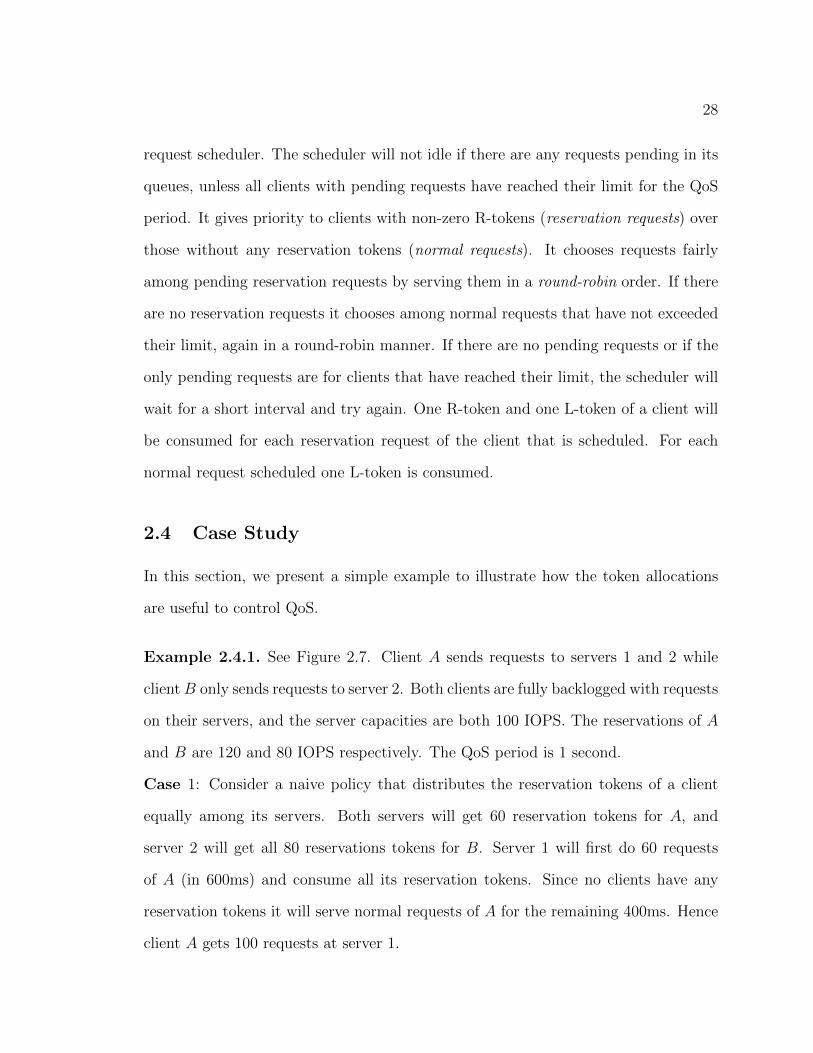
28

request scheduler. The scheduler will not idle if there are any requests pending in its

queues, unless all clients with pending requests have reached their limit for the QoS

period. It gives priority to clients with non-zero R-tokens (reservation requests) over

those without any reservation tokens (normal requests). It chooses requests fairly

among pending reservation requests by serving them in a round-robin order. If there

are no reservation requests it chooses among normal requests that have not exceeded

their limit, again in a round-robin manner. If there are no pending requests or if the

only pending requests are for clients that have reached their limit, the scheduler will

wait for a short interval and try again. One R-token and one L-token of a client will

be consumed for each reservation request of the client that is scheduled. For each

normal request scheduled one L-token is consumed.

2.4 Case Study

In this section, we present a simple example to illustrate how the token allocations

are useful to control QoS.

Example 2.4.1. See Figure 2.7. Client A sends requests to servers 1 and 2 while

clientB only sends requests to server 2. Both clients are fully backlogged with requests

on their servers, and the server capacities are both 100 IOPS. The reservations of A

and B are 120 and 80 IOPS respectively. The QoS period is 1 second.

Case 1: Consider a naive policy that distributes the reservation tokens of a client

equally among its servers. Both servers will get 60 reservation tokens for A, and

server 2 will get all 80 reservations tokens for B. Server 1 will first do 60 requests

of A (in 600ms) and consume all its reservation tokens. Since no clients have any

reservation tokens it will serve normal requests of A for the remaining 400ms. Hence

client A gets 100 requests at server 1.

29

server 2 (100 IOPS)

reservation (B) = 80

reservation (A) = 120

server 1 (100 IOPS)

Figure 2.7 : Illustration of Example 2.4.1.

In contrast, server 2 is over-committed: it received 140 reservation tokens (60 for A

and 80 for B), exceeding its capacity of 100 IOPS. Its scheduler will serve A and B

in a round-robin fashion as long as both have reservation tokens. Hence both clients

get 50 requests. As a result, A gets 150 requests (100 at server 1 and 50 at server 2)

and exceeds its reservation. However, B gets only 50 requests serviced in total and

fails to meet its reservation. Both servers are 100% utilized and do a total of 200

requests, but the naive token allocation fails to meet the reservation of B.

Case 2: An optimal token distribution will allocate all 80 reservation tokens for B

to server 2 (as before), but will only allocate 20 reservation tokens for A to it. The

remaining 100 tokens of A will be allocated to server 1. Now server 2 will complete 80

requests of B and 20 requests of A before it runs out of reservation tokens, while server

1 will do 100 reservation requests of A. Both clients will now meet their reservation

requirements, and both servers are 100% utilized.

2.5 Chapter Summary

In this chapter, we presented the bQueue framework for providing reservation and

limit controls in distributed storage systems. We use tokens to control the number

of reservation requests done for a client at a server, and to cap the maximum num-

30

ber of serviced requests. To accommodate variations in demand and capacity due to

workload changes, token allocations are recomputed at fixed intervals using run-time

estimates of the demand and capacity. The servers use a token-based round-robin

scheduling algorithm to schedule the requests. Compared to fine-grained QoS solu-

tions, we do not have extra overhead for generating metadata with each request at

a centralized ingress node, and require only a simple round-robin scheduler at the

servers. In the next chapter, we formalize the token allocation problem and present

our solutions including the novel pTrans algorithm.

31

Chapter 3

Token Allocation

3.1 Chapter Overview

In this chapter, we formalize the process of token allocation as an optimization prob-

lem. We first present two natural formulations for the problem: an Integer Linear

Program (ILP) and finding the maximum flow (max-flow) in a directed graph. This

is followed by the description of a novel formulation called pTrans. In particular,

pTrans uses a directed graph with vector edge attributes to model the token alloca-

tion problem. It uses an iterative algorithm that successively identifies feasible token

distributions with higher total allocation. A detailed proof in Chapter 4 shows that

pTrans terminates with a globally optimal allocation, and that it has a worst-case

polynomial-time upper bound. Moreover, pTrans can be easily parallelized using mul-

tiple threads, and can be further accelerated using a simple approximation approach.

3.2 Problem Description

We first present a precise description of the token allocation problem. We use the term

client to refer to the entity that receives QoS guarantees, which must be satisfied

within a QoS period as defined in Section 2.2. A client may represent an organization

with multiple users accessing the storage system or, when applied to bucket QoS, a

client may represent a bucket owner who is paying for accesses made to the objects

in the bucket.

32

We use C and S to denote the sets of clients and servers, respectively. A client

i ∈ C may make requests to multiple servers; the demand dji is the number of

requests made by client i to server j. The aggregate demand of client i across all

servers is Di =∑

j∈S dji . Each client i specifies its reservation requirement Ri as

the minimum number of its requests that must receive service in the colorred QoS

period. Without loss of generality, we assume that Di ≥ Ri for all i ∈ C, i.e. a client

has sufficient aggregate demand to meet its reservation. If not, the best the system

can do is to match its demand, so we will temporarily set Ri = Di. Finally, each

server has a capacity upper bound T j equal to the number of requests it can service

during the QoS period.

For each client i, the algorithm allocates some number, aji , of tokens to server

j. The availability of a token implies that the server will serve one request for that

client. We distribute as many of the Ri tokens of client i among the servers based

on capacity and demand constraints. When a server does a request for client i, it

consumes one of its tokens. We assume that servers use a scheduling method that

prioritizes clients with available tokens; these clients are served requests evenly using a

round-robin scheduling policy. If all Ri tokens of client i are consumed, its reservation

requirement will be met.

There are two situations when a server j may have unconsumed tokens. Firstly,

if j is allocated more tokens for client i than its demand (i.e. dji < aji ), then at most

dji tokens of i can be consumed on server j. Secondly, if the total number of tokens

allocated to server j (i.e.∑

i∈C aji ) exceeds its capacity T j, then some tokens will

not be consumed. In the first case, we say that server j has strong excess tokens

for client i, and in the second case we say that server j has weak excess tokens. A

server having weak excess tokens is also said to be overloaded.

The goal of the algorithm is to distribute the tokens so as to maximize the total

33

number of tokens that will be consumed. However, the distribution of demands

on servers may preclude meeting all reservations irrespective of the scheduling or

token allocation method. For instance, a server may become overloaded if all the

demands of several clients are concentrated on it. One cannot redistribute the tokens

to other servers since they do not have demand from these clients. In this case, it is

fundamentally impossible to meet all reservations, and we settle for maximizing the

total number of tokens consumed.

We refer to a configuration of the system by its demand distribution, server ca-

pacities, and token allocations: [dji , T j, aji ] : i ∈ C, j ∈ S. For a given configuration

µ, we define the effective server capacity, φj(µ), to be the number of tokens that

server j will consume: φj(µ) = min(T j, (∑

i∈Cmin(aji , dji )). The effective system

capacity, Φ(µ), is the sum of the effective capacities of individual servers, i.e. Φ(µ)

=∑

j∈S φj(µ). For different configurations, the effective system capacities Φ may be

different, and the goal is to find an allocation that maximizes Φ, which we call an

optimal allocation. Note that the optimal allocation may not be unique.

Example 3.2.1. Table 3.1 shows a system of 2 servers with capacity 100, and two

clients (red and blue) with reservations of 100 each. The demands and token alloca-

tions are shown in the table. Server 1 receives a total of 125 tokens that exceeds its

capacity, so it is overloaded with 25 weak excess tokens. Server 2 has only 75 tokens

so is underloaded. Note that the allocation of a client on any server does not exceed

the corresponding demand on that server, so there are no strong excess tokens. The

effective capacity of server 1 is min(100, (min(75, 150)+min(50, 50))) = 100 which is

its I/O capacity. Similarly, the effective capacity of server 2 is min(100, (min(25, 50)+

min(50, 50))) = 75. The effective system capacity of the configuration is 175. The

blue client meets its reservation but the red client gets only 75 requests served.

34

d1 d2 a1 a2

Red 150 50 75 25Blue 50 50 50 50

Table 3.1 : Configuration of Example 3.2.1, 3.3.1, 3.3.2 and 3.4.1. Servers 1 and 2have capacity 100 each. The red and blue clients have reservation of 100 each. di andai are demand and token allocation on server i.

3.3 Direct Problem Formulations

The preliminary approaches directly model token allocation as a constrained opti-

mization problem, with constraints 1(a), 2(a) and 3(a) discussed in Section 2.3.2.1.

We present an integer linear programming (ILP) approach that directly specifies the

constraints, and a max-flow approach that models the constraints as edge capacities

of a flow graph.

3.3.1 Integer Linear Programming Approach

The token allocation problem can be directly modeled as an integer linear program-

ming (ILP) optimization as described in Algorithm 2.

Algorithm 2: Integer linear-programming formation for the token allocationproblem

Maximize∑

j∈S∑

i∈C aji

subject to ∀i ∈ C,∀j ∈ S, aji ∈ Z+ // integer constraintsand ∀i ∈ C,

∑j∈S a

ji ≤ Ri // reservation specifications

and ∀j ∈ S,∀i ∈ C, aji ≤ dji // demand constraintsand ∀j ∈ S,

∑i∈C a

ji ≤ T j // capacity constraints

Example 3.3.1. The linear programming formalism for Example 3.2.1 is shown in

Algorithm 3. There are two reservation constraints (one for each client), four demand

35

constraints (per client per server), and two capacity constraints (one for each server).

Algorithm 3: Integer linear programming formation for the token allocationof Example 3.2.1

Maximize a1red + a2red + a1blue + a2bluesubject to a1red, a

2red, a

1blue, a

2blue ∈ Z+

and a1red + a2red ≤ 100and a1blue + a2blue ≤ 100and a1red ≤ 150and a2red ≤ 50and a1blue ≤ 50and a2blue ≤ 50and a1red + a1blue ≤ 100and a2red + a2blue ≤ 100

Since ILP is NP-complete [51], one can try to approximate the solution by relaxing

the integer constraints to obtain a near-optimal solution. Algorithm 4 shows one

possible approximation using integer relaxation. It first solves a Linear Programming

(LP) formulation of the problem by removing the integer constraints in Algorithm 2.

Then it allocates the tokens by taking the floor of the result of the LP optimization.

Finally, the remaining unallocated tokens are allocated to servers with spare demands∗

in a greedy manner. Since LP can be solved in polynomial time [52–54], Algorithm 4

is polynomial-time. However, even the LP solution was found to perform very slow

in practice (see Section 5.3.1).

∗We refer dji − aji as the spare demand of client i on server j. The formal definition will be given

later in Section 3.4.2.

36

Algorithm 4: Linear-programming approximation for the token allocationproblem using integer relaxation.

// Solve the LP by removing the integer constraints in Algorithm 2.Maximize

∑j∈S∑

i∈C fji

and ∀i ∈ C,∑

j∈S fji ≤ Ri // reservation specifications

and ∀j ∈ S,∀i ∈ C, f ji ≤ dji // demand constraintsand ∀j ∈ S,

∑i∈C f

ji ≤ T j // capacity constraints

// Allocate the tokens by taking the floor of the LP solution.// For the remaining tokens, allocate them to servers with sparedemands∗.

for each client i dofor each server j do

aji =⌊f ji⌋;

resi = Ri −∑

j∈S aji ;

Allocate resi tokens to servers with spare demands of client i;

3.3.2 Max-flow Approach

We developed a model for token allocation based on a max-flow [55] approach, as

part of the initial bQueue framework [46]. The algorithm first constructs a token

allocation graph, which is a weighted, directed bipartite graph with a vertex for

each client and each server plus a single SOURCE vertex and a single SINK vertex.

The edges of the graph are defined below.

• A directed edge from the SOURCE vertex to each client vertex i, where the

weight of the edge is the reservation Ri.

• A directed edge from each client vertex i to all server vertices j, where the

weight of the edge is the demand dji .

• A directed edge from each server vertex j to the SINK vertex, there the weight

of the edge is the capacity T j.

37

Then by running the max-flow algorithm, flow f ji on edge i, j represents the

number of tokens to be allocated for client i on server j. Since all edges in the token

allocation graph have integer weights, based on the integral flow theorem [55], there

always exists a maximum flow for which the flow on every edge is an integer. This

implies that we can always find an optimal token allocation indicated by flow f ji .

Example 3.3.2. Figure 3.1a shows the token allocation graph for the scenario de-

scribed in Example 3.2.1. The weights on the edges from SOURCE to nodes Red and

Blue represent reservations of 100 for both clients. The edges of weight 100 from

servers 1 and 2 to SINK are the capacities of the servers. Finally, the edges between

the clients and servers indicate the corresponding demands. As shown in Figure 3.1b,

the max-flow has a value of 200, and the individual flows between clients and servers

are all 50, as shown on the edges. Note the optimal allocation may not be unique,

and the max-flow algorithm may give any of them.

Algorithm 5 shows the pseudo-code of the max-flow approach.

Comparing to the NP-complete ILP approach or LP approximation in Section 3.3.1,

the max-flow approach guarantees the optimal solution in polynomial time. However,

max-flow algorithms still have high time complexities and cannot be parallelized,

which makes it impractical to use in storage systems at large scales. This motivates

us to develop a dedicated algorithm for the token allocation problem.

3.4 pTrans Algorithm

In this section, we present a polynomial-time algorithm pTrans which efficiently solves

the token allocation problem. Unlike the LP and max-flow approaches which work

on satisfying constraints, pTrans uses a directed graph with vector edge attributes to

model the allocation problem as a load balancing problem.

38

1

2

100

100

150

50

50100

100

SOURCE SINK50

(a) Token allocation graph.

1

2

100/100

100/100

50/150

50/50

50/50100/100

100/100

SOURCE SINK50/50

(b) Token distribution given by the max-flow algorithm.

Figure 3.1 : Token allocation determined by max-flow approach for Example 3.3.2.

Algorithm 5: Max-flow approach for the token allocation problem

// Build token allocation graph.for each client i do

w(SOURCE, i) = Ri;

for each server j dow(j, SINK) = T j;

for each client i dofor each server j do

w(i, j) = dji ;

// Determine the token allocation by computing the max-flow.Determine the maximum flow from SOURCE to SINK for the token allocationgraph.

Let f ji denote the flow along the edge from client i to server j computed bythe max-flow algorithm.

for each client i dofor each server j do

Allocate f ji tokens for client i to server j;

39

3.4.1 pTrans Algorithm Overview

To find an optimal allocation we only consider prudent allocations in which there

are no strong excess tokens at any server, i.e. the token allocation satisfies aji ≤ dji for

all i ∈ C, j ∈ S. A prudent allocation always exists since∑

j∈S aji = Ri ≤ Di =

∑j d

ji .

It is obvious that an optimal allocation is either prudent or can be transformed to a

prudent allocation with the same Φ.

The algorithm operates as follows. An initial prudent allocation is obtained by

distributing the Ri tokens of client i among the servers in proportion to its demand

on the server, i.e. server j gets an initial allocation of aji = Ri × (dji/Di). Since

Di ≥ Ri, we always have aji ≤ dji , so there are no strong excess tokens in the initial

allocation. Following this allocation some servers may be overloaded, some may be

underloaded, and the rest will exactly match their capacities.

The algorithm then iteratively attempts to find another prudent allocation with

higher Φ by moving tokens from an overloaded server to an underloaded one. We

refer to such a token movement as a prudent transfer. Every token moved in this

way increases Φ by 1. The algorithm stops when there are no overloaded servers or

there are no prudent transfers from an overloaded to an underloaded server possible.

The resulting allocation will be optimal, and the proof is given in Section 4.2.

The pseudo-code in Algorithm 6 shows the overview of pTrans algorithm. There

are three major steps: initial prudent allocation of tokens to the servers (Algorithm 7);

creation of the initial prudent transfer graph (Algorithm 8), discussed in Sec-

tion 3.4.2; iterative improvement of Φ by prudent transfers of tokens from overloaded

to underloaded servers (Algorithm 9), discussed in Section 3.4.3.

40

Algorithm 6: pTrans Algorithm Overview

InitialAllocation();MakePrudentTransferGraph();IterativePrudentTransfers();

Algorithm 7: InitialAllocation Function

for each client i ∈ C do

Di =∑

j∈S dji ;

Ai = min(Di, Ri);

for each client i ∈ C do

aji = Ai × dji/Di;

3.4.2 Prudent Transfer Graph

We first give a clearer definition of prudent transfers. The prudent transfer of tokens

between two servers may be done either directly or indirectly. To effect a direct

transfer, the donor server must have a sufficient number of tokens of some client and

the receiver must have high enough demand for that client to avoid creating strong

excess tokens. Specifically, a prudent transfer of n ≥ 1 tokens of client i from server j

to server k requires: (i) aji ≥ n and (ii) dki − aki ≥ n. We refer to dki − aki as the spare

demand of server k for client i, which indicates the number of tokens of client i that

server k can accept in a prudent transfer.

Example 3.4.1. The token distribution of Example 3.2.1 is an initial prudent allo-

cation in which tokens are distributed in proportion to the demands. Server 1 has 50

blue tokens that it can donate. However, server 2 cannot accept any blue tokens since

it has no spare demand. So no blue tokens can be transferred from server 1 to server

2. On the other hand, server 1 has 75 red tokens it can donate and server 2 has a

spare demand of 25 red tokens. So min75, 25 = 25 red tokens can be transferred

41

d1 d2 d3 a1 a2 a3

Red 150 50 0 75 25 0Blue 0 150 50 0 75 25

Green 50 0 50 50 0 50

Table 3.2 : Configuration of Example 3.4.2. All servers have capacity 100 and allclients have reservation of 100. di and ai are the demand and token allocation forserver i.

from server 1 to 2 resulting in both servers having 100 tokens each. After the transfer,

Φ increases to 200. The reservations of both clients are now satisfied.

We now describe a more complicated example where a direct token transfer is not

possible.

Example 3.4.2. Consider three servers of capacity 100 each and three clients: red,

blue and green. The demands and initial token allocations of the clients are shown in

Table 3.2. Server 1 is overloaded (125), server 3 is underloaded (75) and server 2 is

full (100). The tokens on server 1 and 3 are not compatible: server 1 can donate red

and green tokens but server 3 has no spare demand for either client, and so cannot

accept them in a prudent transfer. On the other hand, server 3 has a spare demand of

25 for blue tokens but server 1 has no blue tokens to donate. Hence direct transferring

tokens from 1 to 3 is not possible. We therefore look for an indirect transfer using

intermediate servers to act as token brokers to create a path of compatible token

transfers. In this example, server 1 can donate 25 red tokens to server 2 in a prudent

transfer; this would make server 2 overloaded, but it can get rid of these 25 weak

excess tokens by transferring 25 blue tokens to server 3. After this brokered transfer,

there are no weak or strong excess tokens and all clients meet their reservations.

When servers j and k do not have compatible donor and receptor tokens an

42

indirect transfer may be possible. In an indirect transfer of tokens from server j to

k, the transfer is effected with the help of intermediate servers u1, u2, · · ·us (called

brokers). A broker accepts a token of some client and sends out a token of another

client. For each of the n tokens transferred from server j to k: j moves a token of

client c0 to server u1 that in turn moves a token of another client c1 to server u2.

Each server ui, 2 ≤ i < s, accepts a token of a client ci−1 from ui−1 and sends a token

of client ci to ui+1. Finally, us sends a token of client cs to server k. If the source

server j is overloaded by at least n tokens and the sink server k is underloaded by at

least n then the above transfer will increase Φ by n.

In the pTrans algorithm, we maintain a data structure called the prudent trans-

fer graph (PTG), which is a weighted directed graph in which each vertex represents

a server. For each pair of servers j and k, there is an associated vector PTj,k called a

prudent transfer vector with |C| components, one for each client. The ith compo-

nent of the vector specifies the number of tokens of client i that can be moved from

j to k directly. From the previous discussion, PTj,k[i] = min(aji , dki − aki ). We also

define the weight of the edge between servers j and k as PTSj,k =∑

i∈C PTj,k[i], the

total number of tokens of all clients that can be moved between the servers directly.

We omit the edge if its weight is 0.

Example 3.4.3. Table 3.3 shows the PT vectors and PTS between each pair of

servers for the configuration of Example 3.4.2. For instance, server 1 can only transfer

25 red tokens to server 2 and cannot transfer any tokens to server 3, hence PT1,2 =

[25, 0, 0] and PTS1,2 = 25. An illustration of the corresponding prudent transfer

graph is shown in Figure 3.2. Note the edges between vertices 1 and 3 have zero

weight and are not shown.

Algorithm 8 shows the initialization of the prudent transfer graph, and the collec-

43

1 2 3

1 - [25, 0, 0] / 25 [0, 0, 0] / 02 [25, 0, 0] / 25 - [0, 25, 0] / 253 [0, 0, 0] / 0 [0, 25, 0] / 25 -

Table 3.3 : Prudent transfer graph for configuration of Table 3.2. Each entry is PTj,k

vector / PTSj,k from server j (row) to server k (column).

1 32[25, 0, 0] / 25

[25, 0, 0] / 25

[0, 25, 0] / 25

[0, 25, 0] / 25

Figure 3.2 : Illustration of prudent transfer graph in Example 3.4.3.

tion of the prudent transfer vectors PTj,k and PTSj,k, for all pairs of servers j, k ∈ S.

Algorithm 8: MakePrudentTransferGraph Function

// Create a prudent transfer vector for each pair of serversfor each j ∈ S do

for each k ∈ S, k 6= j, dofor each i ∈ C do

PTj,k[i] = min(aji , dki − aki );

PTSj,k =∑

i∈C PTj,k[i];

3.4.3 Prudent Token Transfer

After the initialization, pTrans iteratively makes prudent transfers from an overloaded

to an underloaded server until no more prudent transfers can be made, or there are

no overloaded servers. The prudent transfer graph models the prudent transfers

we can do with the current configuration. If there is a directed edge with weight

PTSj,k = w > 0 from an overloaded server j to an underloaded server k, then it is

44

possible to move w tokens from server j to server k so Φ will be increased by w, while

not creating strong excess tokens (i.e. in a direct prudent transfer).

We extend this observation to a simple path of length l ≥ 2 from overloaded server

j to underloaded server k going through intermediate vertices u1, u2, · · ·ul−1. Let the

nonzero weights of the edges in this path be w1, w2 · · ·wl. Denote the smallest weight

on this path by wmin. Then it is always possible to construct a prudent transfer that

moves wmin tokens from j to the k, by moving wmin tokens across each edgein the

path i.e. from j to u1, from ui to ui+1, i = 1, · · · l − 2, and from ul−1 to k. We call

such a path a transfer path, and an illustration is shown in Figure 3.3. Transfer

paths can be found using breadth-first search (BFS) on the prudent transfer graph.

j u1 kul-1u2 ...w1 w2 w3 wl-1 wl

wmin = min w1, w2, w3, ..., wlwmin wmin wmin wmin wmin

Figure 3.3 : Illustration of transfer path.

Note that the number of tokens at any intermediate server ui is not changed by

the prudent transfer, so no weak excess tokens are created at ui. Also, since the

transfer is prudent, no strong excess tokens are created. Hence the effective server

capacity φui of an intermediate server ui does not change.

The effective capacity φj of the source server j will not decrease so long as it

does not become underloaded due to the tokens moved from it. Correspondingly,

the effective capacity φk of the destination server k will increase so long as it does

not become overloaded due to the tokens transferred into it. As a consequence, the

effective system capacity Φ will increase if j is an overloaded server and k is an

underloaded server, and the number of tokens transferred does not cause either j to

45

become underloaded or k to become overloaded.

Therefore, given a transfer path from an overloaded server j to an underloaded

server k, we denote the amount of overload on j (i.e.∑

i∈C aki − T j) by γj, and the

amount of underload on k (i.e. T k −∑

i∈C aki ) by θk. Let wmin denote the smallest

weight of the edges in a chosen transfer path from j to k. We define the transfer

size Ω = minγj, wmin, θk. The algorithm will move Ω tokens along the transfer

path. By construction, the resulting allocation will be prudent and Φ will increase

by Ω.

Moving tokens along the transfer path changes the configuration. Specifically,

each server w in the transfer path may have a change in the allocation awi for one

or more clients i ∈ C. This requires recalculating the prudent transfer vectors of

all outgoing and incoming edges from and to w for those clients i ∈ C whose token

allocations have changed, i.e. PTw,k[i] and PTk,w[i], ∀k ∈ S. This also means that

some edge with zero weight (i.e. not present in the current graph) may have non-

zero weight after the transfer, and will now appear in the graph representing the new

configuration. To bound the complexity of the algorithm we will need to bound the

number of times an edge can (re)appear in the graph.

Algorithm 9 gives a pseudo-code of the iterative prudent transfer function. For

each overloaded server P , it iteratively moves tokens from P to underloaded servers

by exploring transfer paths in increasing order of length. We can show that making

a transfer from P will never generate a shorter transfer path from P to an under-

loaded server. Hence, by performing transfers in increasing order of path lengths,

we can derive a polynomial upper bound on the number of transfers made from P

(see Section 4.3). The algorithm for overloaded server P ends when P is no longer

overloaded or no transfer path can be found from P . For the latter case, we show

in Section 4.2 that when making prudent transfers from other overloaded servers, we

46

Algorithm 9: IterativePrudentTransfers Function

for each overloaded server P dofor l from 1 to (|S| − 1) do

while P is still overloaded and a transfer path from P with length lexists do

Find a transfer path (u0, u1, · · ·ul−1, ul) from server P = u0 to anunderloaded server ul = Q with length l using BFS;

if no transfer path found thenbreak;

Ω = min(γP , θQ);for each pair of adjacent servers (ui, ui+1) on the transfer path do

Ω = min(Ω, wi);

for each pair of adjacent servers (ui, ui+1) on the transfer path doSelect Ω tokens on ui to move to ui+1;Update prudent transfer graph for all edges into and out of uiand ui+1;

will never generate new transfer paths from P .

The algorithm terminates either when there are no overloaded servers or when

there is no transfer path. Since moving tokens along a transfer path will increase Φ,

it is obvious that a globally optimal allocation should not contain any transfer path in

its prudent transfer graph. On the other hand, it can be shown (Section 4.1) that the

converse is also true: i.e. an allocation with no transfer path is optimal. Therefore,

the iterative prudent transfer function will terminate with a globally optimal solution

that maximizes Φ.

3.4.4 Performance Optimizations

3.4.4.1 Parallelizing pTrans

pTrans has the opportunity to achieve better scalability by parallelization. The two

most time-consuming functions are MakePrudentTransferGraph and IterativePru-

47

dentTransfers, and both can be parallelized. The function MakePrudentTransfer-

Graph shown in Algorithm 8, has execution time complexity of O(|S|2|C|). Since this

function is simply initializing a 2D array of vectors whose entries are independent,

this step can be fully parallelized. For instance, we can evenly divide one dimension of

the array into several parts and have different threads working on different subarrays.

In the function IterativePrudentTransfers shown in Algorithm 9, the most time-

consuming step is the update of the Prudent Transfer Graph for each affected server.

The update has a complexity of O(|S||C|). However, the updates can be parallelized

by evenly partitioning the clients, and letting different threads work on updating

entries in its partition.

3.4.4.2 Approximation Approach

Another opportunity to accelerate the pTrans algorithm is to use an approximation

approach. This is based on the observation that not all clients contribute equally in

causing overload or reducing underload. In particular, clients with a small number of

tokens and those with only a small amount of spare demand do not contribute much

to increasing Φ.

Therefore, instead of maintaining a vector of size |C| for each edge, pTrans need

only consider the clients with the top M (or fraction f) token counts and spare

demands. Then the controller only considers the reduced information for the prudent

transfers. In practice, we found that in most cases we only need a small fraction of

the clients to achieve the optimal or near-optimal Φ (see Section 5.4). We leave for

future work an analysis of such an approximation scheme.

48

3.4.5 Comparing pTrans with Preliminary Approaches

In this section, we compare pTrans with the LP and max-flow formulations of the

problem, and show the advantages of pTrans. Furthermore, experimental comparisons

of the methods are presented in Section 5.3.1.

The ILP approach has the same goal as pTrans: maximizing the number of reser-

vations that can be met. However, this formulation requires O(|S||C|) inequalities

to model the per-client per-server demand constraints. Since ILP is NP-complete it

makes an efficient exact solution unlikely. Furthermore, even an approximate LP for-

mulation using integer relaxation has a poor running time. In contrast, in Section 4.3,

we prove that pTrans is able to find the optimal allocation in polynomial-time, and

our experiments show that it runs fast in practice.

Similarly, the max-flow approach works on graphs with per-server, per-client infor-

mation simultaneously, which results in a graph of O(|S||C|) edges, which is especially

poor for the typical situation in which |C| >> |S|. In contrast, pTrans has a much

smaller overhead by modeling the token allocation as a two-level problem. It first

works on the prudent transfer graph which only includes servers (whose number of

vertices is O(|S|)) to find out the shift path, and then figures out which clients’ tokens

to move.

3.5 Chapter Summary

In this chapter, we formalized the token allocation problem and presented three token

allocation algorithms. Apart from the direct formulations using ILP and max-flow,

the major contribution is a novel approach embodied in pTrans, a fast and scalable

algorithm for handling token allocation. pTrans models the problem as distribut-

ing tokens on a small graph (the number of vertices equals the number of servers)

49

augmented with per-edge vectors with client information. pTrans greedily transfers

tokens from overloaded to underloaded servers while avoiding the creation of wasteful

strong-excess tokens. pTrans has a much smaller runtime overhead than the other

approaches considered. It can be further accelerated using parallelization and ap-

proximation mechanisms.

In the next chapter, we formally prove that pTrans always results in an optimal

allocation, and converges to the global optimal solution in a polynomial number of

steps. In Chapter 5, we experimentally show that pTrans handles distributed token

allocation effectively, and outperforms the other methods by a large margin.

50

Chapter 4

Analysis of pTrans Algorithm

In this chapter we present formal proofs of correctness and analysis of the time com-

plexity of pTrans [48].

4.1 Fundamental pTrans Optimality Theorem

In this section, we show the fundamental pTrans optimality theorem, which

states that an allocation is optimal if and only if it has no transfer path in its prudent

transfer graph. By using this theorem, we show in the next section that pTrans always

terminates with the optimal token allocation. To prove this theorem, we show that

an allocation is non-optimal if and only if it has a transfer path in its

prudent transfer graph. Moreover, since the input allocation of pTrans is prudent

and pTrans always keeps the allocations prudent, all allocations in this section will

be assumed to be prudent, i.e. satisfy ∀i ∈ C, j ∈ S, aji ≤ dji .

First of all, the ’if ’ part is trivial to show.

Theorem 1. An allocation µ which contains a transfer path in its prudent transfer

graph is non-optimal.

Proof. For an allocation µ with a transfer path, we can find another allocation µ′

with higher Φ by moving Ω tokens (the transfer size) along the transfer path. This

increases Φ by Ω. Thus, the allocation µ is not optimal.

Next we show the ’only if ’ part. We establish some elementary properties of the

51

token distribution in a non-optimal allocation, followed by an inductive argument in

Lemma 6 that a non-optimal allocation must have a transfer path. Firstly, given an

allocation µ, we recall the three states of the servers. A server j is said to be

• overloaded if the number of tokens allocated to it exceeds its capacity, i.e.∑i∈C a

ji > T j.

• full if the number of tokens allocated to it equals to its capacity, i.e.∑

i∈C aji =

T j.

• underloaded if the number of tokens allocated to it is less than its capacity,

i.e.∑

i∈C aji < T j.

Lemma 2. For a non-optimal allocation µ, ∃s ∈ S where s is overloaded, i.e.∑i∈C a

si > T s.

Proof. Assume no server is overloaded, i.e. ∀j ∈ S, we have∑

i∈C aji ≤ T j. Then for

any server j, its effective server capacity will be

φj(µ) = min(T j,∑i∈C

aji ) =∑i∈C

aji (4.1)

i.e. φj(µ) equals the total number of tokens allocated to server j. Then the effective

system capacity will be

Φ(µ) =∑j∈S

φj(µ) =∑j∈S

(∑i∈C

aji ) =∑i∈C

(∑j∈S

aji ) =∑i∈C

Ri (4.2)

i.e. Φ(µ) equals the sum of the reservations of all clients. This means that all

reservations will be met and thus µ is optimal, which contradicts our assumption.

Lemma 3. For a non-optimal allocation µ, ∃t ∈ S where t is underloaded, i.e.∑i∈C a

ti < T t.

52

Proof. Assume no server is underloaded, i.e. ∀j ∈ S, we have∑

i∈C aji ≥ T j. Then

for any server j, its effective server capacity will be

φj(µ) = min(T j,∑i∈C

aji ) = T j (4.3)

i.e. φj(µ) equals the capacity of server j. Then the effective system capacity will be

Φ(µ) =∑j∈S

φj(µ) =∑j∈S

T j (4.4)

i.e. Φ(µ) equals the total capacity of all servers. This means all servers’ capacities

will be utilized and thus µ is optimal, which contradicts our assumption.

Hence, according to Lemma 2 and Lemma 3, for a non-optimal allocation µ, the

server set S can be partitioned into two non-empty subsets SOF(µ) and SU(µ), where

SOF(µ) consists of all overloaded and full servers and SU(µ) consists of all underloaded

servers in µ. We will refer to the sum of the effective server capacities for a subset of

servers W as the effective capacity of W .

Lemma 4. Given a non-optimal allocation µ and its corresponding partition SOF(µ)

and SU(µ), any optimal allocation µ∗ will have a higher value for the effective capacity

of SU(µ), i.e.∑

j∈SU(µ) φj(µ∗) >

∑j∈SU(µ) φ

j(µ).

Proof. Firstly, since µ∗ is optimal and µ is non-optimal, we have

Φ(µ∗) > Φ(µ) (4.5)

53

Then by the definition of effective system capacity, we have

Φ(µ) =∑j∈S

φj(µ) =∑

j∈SOF(µ)

φj(µ) +∑

j∈SU(µ)

φj(µ) (4.6)

and

Φ(µ∗) =∑j∈S

φj(µ∗) =∑

j∈SOF(µ)

φj(µ∗) +∑

j∈SU(µ)

φj(µ∗) (4.7)

Moreover, all servers in SOF(µ) are fully utilized (hence their effective server capacities

are maximized) in µ. Thus, we have

∑j∈SOF(µ)

φj(µ) =∑

j∈SOF(µ)

T j ≥∑

j∈SOF(µ)

φj(µ∗) (4.8)

By combining Equations (4.5) (4.6) (4.7) (4.8), we have

∑j∈SU(µ)

φj(µ∗) >∑

j∈SU(µ)

φj(µ) (4.9)

Using Lemma 4, we can further derive the following lemma, which forms the basic

requirement for a prudent transfer.

Lemma 5. Given a non-optimal allocation µ and its corresponding partition SOF(µ)

and SU(µ), ∃i ∈ C, s ∈ SOF(µ) and t ∈ SU(µ), such that in µ, i has token(s) on s

and spare demand(s) on t.

Proof. Assume such an i does not exist, i.e. all clients having spare demands (if any)

in SU(µ) do not have any tokens in SOF(µ). Then consider the effective capacity

of SU(µ). Since all servers in SU(µ) are underloaded, i.e. there are no weak excess

tokens,∑

j∈SU(µ) φj(µ) will be equal to the number of tokens of all clients allocated

54

in SU(µ),i.e. we have ∑j∈SU(µ)

φj(µ) =∑i∈C

(∑

j∈SU(µ)

aji ) (4.10)

For each client i, there are two cases.

• If i does not have spare demand in SU(µ), which means the number of tokens

of i allocated in SU(µ) is exactly same as the total demand of i in SU(µ). Then∑j∈SU(µ) a

ji =

∑j∈SU(µ) d

ji , which cannot be increased in any other allocation.

• If i has spare demand in SU(µ), then according to the assumption, there are no

tokens of i allocated in SOF(µ). This means that all tokens of i are allocated in

SU(µ), which implies that∑

j∈SU(µ) aji = Ri. This also cannot be increased in

any other allocation.

Therefore, for any client i, the value∑

j∈SU(µ) aji in Equation 4.10 cannot be increased

in any other allocation. This means∑

j∈SU(µ) φj(µ) is maximized in the non-optimal

allocation µ, which contradicts Lemma 4.

Now by using induction, we can show a transfer path must exist in the prudent

transfer graph of any non-optimal allocation.

Theorem 6. Given a non-optimal allocation µ, a transfer path exists in its prudent

transfer graph.

Proof. Let SOF(µ) and SU(µ) be the server partitions of µ as defined earlier. We use

induction on |SOF(µ)| to show that a transfer path must exist.

• If |SOF(µ)| = 1, then according to Lemma 2, SOF(µ) must contain one over-

loaded server, say s0. Then by Lemma 5, ∃i ∈ C and s1 ∈ SU(µ) such that i

has token(s) on s0 and has spare demand(s) on s1. This implies a transfer path

s0, s1 exists (i.e. a direct transfer) that establishes the base of the induction.

55

• Suppose a transfer path exists for all non-optimal allocations with |SOF| =

K. Consider a non-optimal allocation µ where |SOF(µ)| = K + 1. Then, by

Lemma 5, there are two situations.

– If ∃i ∈ C which has token(s) on an overloaded server s0 ∈ SOF(µ) and

has spare demand(s) on s1 ∈ SU(µ), then it implies a direct transfer path

s0, s1 exists.

– If @i ∈ C that has token(s) on an overloaded server in SOF(µ) and has spare

demand(s) on a server in SU(µ), then it means ∃i ∈ C which has token(s)

on a full server s0 ∈ SOF(µ) and has spare demand(s) on s1 ∈ SU(µ).

Then consider the configuration µ′ which is same as µ but in which s0’s

capacity is increased by 1. Note µ′ should also be non-optimal (otherwise

µ will also be optimal since the extra capacity 1 added on s0 will not help

increasing Φ), and s0 is underloaded in µ′, i.e. SU(µ′) = s0∪SU(µ) and

|SOF(µ′)| = K. According to the induction assumption, a transfer path

s′0, s′1, · · · s′n−1, s′n exists in µ′. Then we can always find another transfer

path in µ:

∗ If ∃k ∈ C where s′k = s1, then s′0, s′1, · · · s′k−1, s′k = s1 is also a

transfer path in µ.

∗ If @k ∈ C where s′k = s1, and s′n 6= s0, then s′0, s′1, · · · s′n−1, s′n is also

a transfer path in µ.

∗ If @k ∈ C where s′k = s1, and s′n = s0, then we can form a transfer

path s′0, s′1, · · · s′n−1, s0, s1 in µ.

Therefore, a transfer path always exists for non-optimal allocations.

Finally, according to Theorems 1 and 6, we have the following conclusion, which

56

P j k u

s'm-1s'0

s'n

tokens of client i

(a) Case (1) and (3).

P j k u

s'm+1

s'0

s'n

tokens of client i

(b) Case (2).

Figure 4.1 : Illustration of base cases in the proof of Theorem 8. The green edgesindicate the prudent transfer made, and the dotted edge indicates the new edge j, kgenerated after making the transfer.

is the fundamental pTrans optimality theorem.

Theorem 7. An allocation is optimal if and only if it has no transfer path in its

prudent transfer graph.

4.2 Correctness of pTrans

We now show that when the pTrans algorithm specified in Algorithm 9 terminates

there will be no transfer paths in the prudent transfer graph. Then Theorem 7 implies

that its allocation is optimal. Since Algorithm 9 is performed server by server in the

outer loop, we must show that after the algorithm completes its iteration for some

overloaded server P , no new transfer paths starting from P will be generated in

subsequent iterations. Hence when the algorithm terminates, there are no transfer

paths and the allocation is optimal.

Before giving the proof, we first discuss the situations in which new edges can

be generated in the prudent transfer graph. Suppose that after making a transfer, a

new edge j, k from server j to server k is generated. Recall the definition of the

edge weight: PTSj,k =∑

i∈C PTj,k[i] and PTj,k[i] = min(aji , dki − aki ). Since PTSj,k

57

changed from 0 to some non-zero value, there must exist a client i for which PTj,k[i]

increased, i.e., min(aji , dki − aki ) increased. Then there are three cases:

1. ∃i ∈ C, whose token allocation on j increased from 0 (i.e. aji increased), and

the spare demand on k was positive.

2. ∃i ∈ C, whose token allocation on j was positive, and the spare demand on k

increased from 0, (i.e. dki − aki increased, hence aki decreased).

3. Both changes in (1) and (2) occurred, i.e. aji increased and aki decreased.

The following theorem shows that after Algorithm 9 completes an iteration for

an overloaded server P , no new transfer path from P will be subsequently generated.

This validates the correctness of the greedy per-server approach.

Theorem 8. Consider an allocation µ in which there is no transfer path with P ∈ S

as the source. Then making prudent transfers from other overloaded servers will never

generate new transfer paths from P .

Proof. We show that no new path from P is generated following a single prudent

transfer from some other overloaded server. Suppose, to the contrary, that a new

transfer path π = s0 = P, s1, · · · sn−1, sn is generated after making a prudent trans-

fer from some other overloaded server s′0. Then there must be at least one new edge

in π which did not exist in µ. Let si = j, si+1 = k be the first of such new edges.

For each of the three situations identified above we derive a contradiction:

• If case (1) or case (3) occurs, it means tokens of client i were moved to server

j in the transfer π′ from s′0, shown by

π′ = s′0, s′1, · · · s′m−1, j, s′m+1, · · · s′n in Figure 4.1a. Then we can form another

transfer path from P in µ as

s0 = P, · · · si−1, j, s′m+1, · · · s′n, which is a contradiction.

58

• If case (2) occurs, it means tokens of i were moved out of server k in the transfer

π′ from s′0, shown by

π′ = s′0, s′1, · · · s′m−1, k, s′m+1, · · · s′n in Figure 4.1b. Since s′m+1 is receiving

tokens of i from k, it must have spare demand of i in µ. On the other hand, by

hypothesis, j has tokens of i in µ: this means the edge from j to s′m+1 exists in

µ. Then we can form another transfer path s0 = P, · · · si−1, j, s′m+1, · · · s′n in

µ, which is a contradiction.

Therefore, no new transfer path from P can be generated after making a prudent

transfer from another source.

Theorems 7 and 8 show that greedily increasing the effective system capacity by

exploiting transfer paths in an arbitrary per-server order, does lead to an optimal

solution.

4.3 Polynomial Bound of pTrans

In this section, we derive a polynomial upper bound for the pTrans algorithm. To this

end, we show that the transfers from a fixed overloaded source server P (i.e. each

outermost iteration in Algorithm 9) can be performed efficiently, by bounding the

number of times any edge can be regenerated in the prudent transfer graph. Given

an allocation µ, we use δµ(j, k) to denote the shortest distance (i.e. the number of

edges in the shortest path) between vertices j and k. The following theorem bounds

the number of times an edge can be regenerated and hence bounds the number of

transfers made by any source server.

Theorem 9. Consider a configuration µ with the source server P . Suppose a prudent

transfer π is made and let µ′ be the resulting configuration. Then in µ′, ∀q ∈ S, any

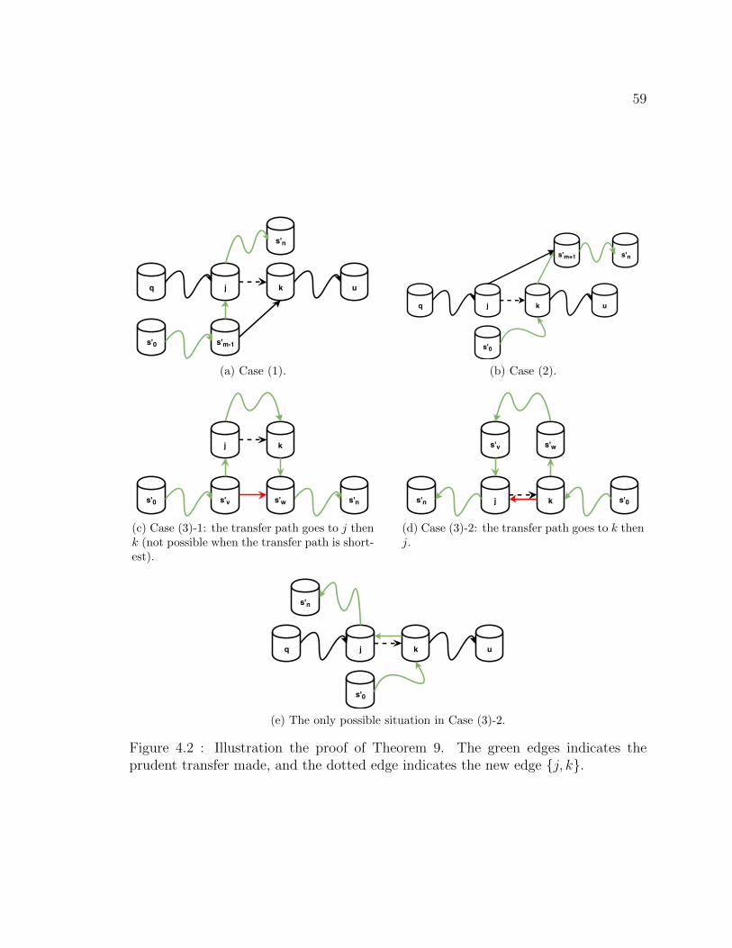
59

q j k u

s'm-1s'0

s'n

(a) Case (1).

q j k u

s'm+1

s'0

s'n

(b) Case (2).

j k

s'vs'0 s'ns'w

(c) Case (3)-1: the transfer path goes to j thenk (not possible when the transfer path is short-est).

s'v s'w

js'n s'0k

(d) Case (3)-2: the transfer path goes to k thenj.

q j k u

s'0

s'n

(e) The only possible situation in Case (3)-2.

Figure 4.2 : Illustration the proof of Theorem 9. The green edges indicates theprudent transfer made, and the dotted edge indicates the new edge j, k.

60

path π′ from q to an underloaded server that includes a new edge will have length

> distµ(q). Note that π′ may not be a transfer path if q is not overloaded.

Proof. We prove the Theorem by induction on the number of new edges in the path

π′ and we use j, k to denote the first new edge in π′.

• Base Case: π′ contains the only one new edge j, k. In this case, in π′, all

edges from q to j, as well as k to u, are old edges that also existed in µ. Hence

we have:

δµ′(q, j) ≥ δµ(q, j) (4.11)

and

δµ′(k, u) ≥ δµ(k, u) (4.12)

Then referring to the analysis of three cases when a new edge was generated (in

Section 4.2):

– If case (1) occurs, it means tokens of some client i were moved to j in π.

Then the transfer path of π can be represented as s′0, · · · s′m−1, j, s′m+1, · · · s′n,

as shown in Figure 4.2a. Since s′m−1 was sending tokens of i to j, it must

have tokens of i in µ. On the other hand, it is assumed that k has spare

demand of i in µ, then it means the edge from s′m−1 to k exists in µ.

Then by the definition of dist, we have:

distµ(q) ≤ δµ(q, j) + δµ(j, s′n) (4.13)

On the other hand, since the transfer path from s′m−1 to s′n was a shortest

one, it means:

δµ(s′m−1, s′n) = δµ(j, s′n) + 1 ≤ δµ(k, u) + 1 (4.14)

61

Then by combining Equations (4.11) (4.12) (4.13) (4.14), we conclude that:

distµ(q) < δµ′(q, j) + δµ′(k, u) + 1 (4.15)

where δµ′(q, j) + δµ′(k, u) + 1 is the length of the path π′.

– If case (2) occurs, it means tokens of some client i were moved away from

k in the transfer. Then the transfer path of π can be represented as

s′0, · · · s′m−1, k, s′m+1, · · · s′n, as shown in Figure 4.2b. Since s′m+1 was re-

ceiving tokens of i from k, it must have spare demand of i in µ. On the

other hand, it is assumed that j has tokens of i in µ, then it means the

edge from j to s′m+1 exists in µ.

Then by the definition of dist, we have:

distµ(q) ≤ δµ(q, j) + 1 + δµ(s′m+1, s′n) (4.16)

On the other hand, since the transfer path from k to s′n was a shortest one,

it means:

δµ(k, s′n) = δµ(s′m+1, s′n) + 1 ≤ δµ(k, u) (4.17)

By combining Equations (4.11), (4.12), (4.16) and (4.17), we conclude

that:

distµ(q) < δµ′(q, j) + δµ′(k, u) + 1 (4.18)

where δµ′(q, j) + δµ′(k, u) + 1 is the length of the path π′.

– If case (3) occurs, it means tokens of some client i were moved to j and

moved away from k in the transfer. Then the transfer path of π be repre-

sented as either

62

Case(3)− 1: s′0, · · · s′v, j, · · · , k, s′w, · · · s′n (Figure 4.2c), or

Case(3) − 2: s′0, · · · k, s′w, · · · , s′v, j, · · · s′n (Figure 4.2d). Case(3) − 1 is

not possible, because in µ, s′v has tokens of i and s′w has spare demand

of i, we can form a shorter transfer path s′0, · · · s′v, s′w, · · · s′n. For the

same reason, the only possible situation in Case(3)− 2 is k directly moved

tokens of i to j, as shown in 4.2e, because otherwise s′0, · · · k, j, · · · s′n is

a shorter transfer path.

Then by the definition of dist, we have:

distµ(q) ≤ δµ(q, j) + δµ(j, s′n) (4.19)

On the other hand, since the transfer path from k to s′n) was a shortest

one, it means:

δµ(k, s′n) = δµ(j, s′n) + 1 ≤ δµ′(k, u) (4.20)

By combining Equations (4.11), (4.12), (4.19) and (4.20), we conclude

that:

distµ(q) < δµ′(q, j) + δµ′(k, u) + 1 (4.21)

where δµ′(q, j) + δµ′(k, u) + 1 is the length of the path π′.

• Inductive Step: for the induction, suppose the statement is true for all paths

from any vertex q to some underloaded server in µ′ with K new edges. Then

consider a path π′ from q to some underloaded server in µ′ with K + 1 new

edges. Then since j, k is the first new edge in π′, all edges from q to j are old

edges that also existed in µ. Hence we have:

δµ′(q, j) ≥ δµ(q, j) (4.22)

63

On the other hand, since the sub-path from k to u contains K new edges, based

on the induction hypothesis, we have:

δµ′(k, u) > distµ(k) (4.23)

Again, referring to the analysis of three cases when a new edge was generated

(in Section 4.2):

– If case (1) (Figure 4.2a) occurs, by the definition of dist, we have:

distµ(q) ≤ δµ(q, j) + δµ(j, s′n) (4.24)

On the other hand, since the transfer path from s′m−1 to s′n was a shortest

one, it means:

δµ(s′m−1, s′n) = δµ(j, s′n) + 1 ≤ distµ(k) + 1 (4.25)

By combining Equations (4.22) (4.23) (4.24) (4.25), we conclude that:

distµ(q) < δµ′(q, j) + δµ′(k, u) + 1 (4.26)

where δµ′(q, j) + δµ′(k, u) + 1 is the length of the path π′.

– If case (2) (Figure 4.2b) occurs, by the definition of dist, we have:

distµ(q) ≤ δµ(q, j) + 1 + δµ(s′m+1, s′n) (4.27)

On the other hand, since the transfer path from k to s′n) was a shortest

64

one, it means:

δµ(k, s′n) = δµ(s′m+1, s′n) + 1 = distµ(k) (4.28)

By combining Equations (4.22), (4.23), (4.27) and (4.28), we conclude

that:

distµ(q) < δµ′(q, j) + δµ′(k, u) + 1 (4.29)

where δµ′(q, j) + δµ′(k, u) + 1 is the length of the path π′.

– If case (3) (Figure 4.2e) occurs, by the definition of dist, we have:

distµ(q) ≤ δµ(q, j) + δµ(j, s′n) (4.30)

On the other hand, since the transfer path from k to s′n) was a shortest

one, it means:

δµ(k, s′n) = δµ(j, s′n) + 1 = distµ(k) (4.31)

By combining Equations (4.22), (4.23), (4.30) and (4.31), we conclude

that:

distµ(q) < δµ′(q, j) + δµ′(k, u) + 1 (4.32)

where δµ′(q, j) + δµ′(k, u) + 1 is the length of the path π′.

Finally, by treating the source server P as the vertex q in Theorem 9, we can

immediately derive Theorem 10.

Theorem 10. Consider a configuration µ with the source server P . Suppose a pru-

dent transfer π is made on a path of length l and let µ′ be the resulting configuration.

65

Then in µ′ any new edge generated by the transfer can only occur in a transfer path

from P of length greater than l.

Finally, the following theorem can be used to derive a polynomial upper bound of

pTrans algorithm.

Theorem 11. In pTrans, for each source server P , the number of prudent transfers

can be made is bounded by O(|S3|).

Proof. Each time when making the shortest prudent transfer with length l in µ, one

of the following scenarios will happen:

1. P become full or underloaded, this happens when the transfer size Ω = γP .

When this happens, we are done for P . Thus, this scenario can only happen

once for each source server P .

2. The underloaded server U in the transfer becomes full, this happens when trans-

fer size Ω = θU . When this happens, U becomes full and will be full for the rest

of the pTrans algorithm. Thus, this scenario can only happen O(|S|) times for

all source servers.

3. An edge j, k on the transfer path gets removed, this happens when transfer

size Ω = wmin. Based on Theorem 10, when j, k reappears in a later configu-

ration µ′, all transfer paths from P to underloaded servers including j, k will

have distance > l. This implies that an edge can be removed then reappear

at most O(|S|) times. Since the number of edges is bounded by O(|S2|), this

scenario can happen at most O(|S3|) times for each source server.

Therefore, for each source server P , the number of prudent transfers can be made is

bounded by O(|S3|).

66

4.4 Comparing pTrans with Edmonds–Karp Algorithm

The Edmonds–Karp [56] algorithm for finding the max-flow have some similarities

with pTrans. Both works on directed graphs, and greedily keep finding profitable

paths (prudent transfer path and augmenting path respectively) until no further progress

is possible. The max-flow min-cut theorem establishes the optimal configuration

for the Edmonds–Karp. An analogous result is the fundamental pTrans optimal-

ity theorem that characterizes the optimal configuration for pTrans, especially the

idea using BFS.

However, there are also some differences between pTrans and Edmonds–Karp.

Unlike Edmonds–Karp which works on the residual graph, pTrans works directly on

the prudent transfer graph, which indicates the number of tokens can be transferred

between servers. Moreover, unlike flows, the edge weights in pTrans cannot be added

or split. For example, server A may be able to give 50 tokens to server B and 50

tokens to server C, but it may not be able to do both.

67

Chapter 5

Evaluation of Bandwidth Allocation QoS

5.1 Experimental Setup

To evaluate the performance of distributed bandwidth allocation QoS, we imple-

mented the QoS framework using both simulation and direct evaluation on a small

Linux cluster. For the former, we create a set of concurrent processes to simulate the

storage servers and the token controller, and use a request generator process at each

server to create the dynamic workload. The communication overhead is simulated by

a built-in delay function. I/O service times are randomly drawn from a uniform dis-

tribution with mean equal to the reciprocal of the server IOPS capacity and limited

variance.

For the actual implementation, we built a prototype on a small cluster of 9 Linux

servers connected using QDR InfiniBand (40 Gb/s). Each server node is equipped

with an Intel R© Xeon R© Processor E5-2640 v4 [57] CPU with 10 two-way hyper-

threaded cores. In our implementation, one thread on each server is responsible for

inserting the generated requests to the client queues. A second thread at the server

runs the Token Scheduler that implements the round-robin scheduling policy. Finally,

each storage node uses an independent thread to communicate with the controller

node. We use the send and recv primitives from the socket programming library to

handle the communication between the controller and the storage nodes, and OpenMP

interface to implement the parallel threads.

Two backend servers were used in the evaluation. The first is the well-known

68

distributed memory caching system memcached [58] and the second is a conventional

block-based Linux storage server. In the first case, each server runs a Memcached

daemon that is pre-populated with 10, 000 objects of size 4KB each. The requests on

each server are generated by an independent YCSB workload generator [59], which

generates the core workload A [60] that gives a 50 − 50 mix of gets and puts. An

initial profile run was used to determine that each server had an average throughput

of roughly 50, 000 requests per second (RPS). All clients are continuously backlogged

on their active servers with 5 outstanding requests. The scheduler chooses requests

from the client queues and invokes the memcahced server with a get or put command.

For the storage backend, requests consist of random 4KB reads from a 1GB file created

on the server. Using 5 concurrent request threads, each server is initially profiled and

found to have an average throughput of roughly 1000 IOPS.

We describe our experimental results below. In Section 5.2 we show that pTrans

can meet reservations and enforce limits in the face of dynamically changing workloads

and large numbers of clients. In Section 5.3 we report the measured run times of the

parallelized controller algorithm on the Linux server for different numbers of threads

and clients. In Section 5.4 results on the tradeoff between run times and accuracy

for the approximation controller algorithm on the Linux server are reported. In

Section 5.5 we show how inaccurate demand estimation could be resolved at runtime.

Finally in Section 5.6 we report the results of the evaluation on Linux scheduler to

show the workings of the pTrans approach in a real system.

69

5.2 QoS Evaluation

5.2.1 Bandwidth Allocation at Large Scale

We use the simulator to show how pTrans handles reservation QoS with a large

number of clients and a dynamically changing workload. There are 64 servers and

10, 000 clients. Each server has an average capacity of 20, 000 IOPS, and we run

the pTrans algorithm for a full QoS period of 5sec; the throughput per QoS period is

therefore roughly 100, 000 I/Os. We divide each QoS period into 5 token redistribution

intervals i.e. a token redistribution is triggered every 1sec using statistics gathered

for the last interval.

Each server’s throughput of 100, 000 I/Os (per QoS period) is fully reserved by

all the clients. This causes the greatest stress on the scheduler since there is no spare

capacity that can compensate for errors in the token distribution. The reservation

of the clients follows a Zipf distribution with an exponent factor s = 0.5, as shown

in Figure 5.1a. The Zipf distribution simulates a common scenario in practice where

most clients have a relatively low reservation while a few highly-active clients have a

much higher reservation. In the figure, there is a factor of 100 between the highest and

lowest reservations. All clients are assumed to have unbounded limits. Each client is

active on 8 servers at any time. The total demand of a client is set to 1.5 times to its

reservation. The average request arrival rate for the client over all servers is the total

demand divided by the length of the QoS period. To stress the pTrans algorithm,

the demands of each client are also distributed among the eight servers using a Zipf

distribution with an exponent factor of s = 0.5. I/O requests for a client on a server

are generated at a uniform rate proportional to the demand on the server. Clients

may change their demands at random times within the QoS period. When a demand

change is triggered, the client randomly selects eight servers (which may or may not

70

intersect with the current set), and redistributes the total demand to them based on

a Zipf distribution. In the initial experiment, a client may change its demands up to

2 times in the QoS period. Figure 5.1b shows the times of demand changes of the

sample of the clients. For instance, client 6100 has its first demand change early in

the 1st interval (around 0.065s).

Figure 5.2 shows the number of requests being completed by all clients in each of

the redistribution intervals. From the figure we can see that, as expected, the number

of requests completed by a client at the end of the last interval is highly consistent

with its reservation. Quantitatively, 99.5% of the clients meet at least 95% of their

reservation. Furthermore, since the servers perform reservation requests in a round-

robin fashion, clients with smaller reservations will complete earlier and free up server

capacity for use by clients with larger reservations. The effect can be seen clearly in

the figure, where during the last two intervals, the servers are mainly processing

requests of the clients with smaller indexes (i.e. those with higher reservations).

Figure 5.2 also shows the adaptivity of the algorithm to sharp demand changes.

For instance, several red needles (representing I/Os in the 2nd interval) can be seen

in the blue (1st interval) region. This means that these clients received less service

than their peers in the first interval. This happens because of a sudden drop in the

demands of this client at some servers and an increase in others because of locality

changes. Servers with reduced demand will not be able to consume their reservation

tokens in this interval. The unused capacity however is not wasted and will be used

by clients which have both demand and tokens on the server.

Even if all tokens with demand at the server have been consumed, the additional

capacity is used to serve requests without tokens. These opportunistic requests will

still be counted towards the reservation requirements of the corresponding client, and

the controller will correct for these additional I/Os by reducing its target remaining

71

100

1000

10000

Res

erva

tion

s

1

10

100

0400

800

1200

1600

2000

2400

2800

3200

3600

4000

4400

4800

5200

5600

6000

6400

6800

7200

7600

8000

8400

8800

9200

9600

Res

erva

tion

s

Client ID

(a) The Zipf distribution of clients’ reservation requirements with theexponent factor s = 0.5, sorted from high to low. Each client is as-signed a weight wi = 1/i0.5 from the set of weights wj : j = 1, · · · |C|with probability (1/i0.5)/(

∑i 1/i0.5). Then the aggregate capacity of

the servers is distributed to the clients in proportional to their weightsas their reservations. The client reservations are roughly in the range of(120, 13000), and the y-axis has a logarithmic scale.

3

4

5

6

Tim

e (s

)

Time of 1st demand changeTime of 2nd demand change

0

1

2

3

040

080

012

0016

0020

0024

0028

0032

0036

0040

0044

0048

0052

0056

0060

0064

0068

0072

0076

0080

0084

0088

0092

0096

00

Tim

e (s

)

Client ID

(b) The time that demand changes of the clients.

Figure 5.1 : The specifications of the simulator-based QoS evaluation: reservationsand demand change times for a sample of the clients. The figures show the resultsfor every 50th client.

72

100

1000

10000

Nu

m o

f R

eque

sts

Don

e

Redistribution Interval 5Redistribution Interval 4Redistribution Interval 3Redistribution Interval 2Redistribution Interval 1

1

10

1000

400

800

1200

1600

2000

2400

2800

3200

3600

4000

4400

4800

5200

5600

6000

6400

6800

7200

7600

8000

8400

8800

9200

9600

Nu

m o

f R

eque

sts

Don

e

Client ID

Figure 5.2 : The number of requests completed for each client in the 5 redistributionintervals. Each client is active (having non-zero demand) on a set of 8 servers. Thefigures show the results for every 50th client.

reservation. In the next interval, the coordinator will allocate additional tokens to

the clients that were underserved in the first interval and direct them to the new

server, and reduce the total number of tokens to clients which received opportunistic

I/Os. For instance, client 6100 that has its first demand change early in the 1st

redistribution interval, receives less service in the first interval but catches up by the

end of the second one.

5.2.2 Effect of Different Parameters

In this experiment we study the effect of two parameters on QoS accuracy: the number

of servers on which the clients are active (NA) and the number of times the demand

of a client changes in a QoS period (ND). The accuracy measure is the fraction of

clients that miss 5% or more of their reservation in the QoS period.

73

Inaccuracy in the reservations achieved may arise due to intrinsic error. The

intrinsic error arises because for certain data distributions it is impossible to meet the

reservations irrespective of the scheduling strategy. For example, consider a situation

where two clients with reservations of 100 IOPS each have a high demand on a single

server and no demand on any of the other servers. If the capacity of the server is

100 IOPS then clearly at most one of the clients can meet its reservation, and the

intrinsic error is greater than 0. Intrinsic errors are manifested in pTrans as weak

excess tokens on some overloaded server(s) that cannot be moved to any underloaded

server because of a lack of demand for the clients on the latter. When there is no

runtime demand change, pTrans guarantees that all reservations will be met whenever

such an allocation is possible. Hence, any error in this situation is an intrinsic error

that cannot be avoided.

Figure 5.3 also shows the average measured error for NA = 2, 4, 8 and ND =

0, 1, 2, 5, 10. Each bar is the average of 5 runs; the variation was less than 10%.

We found the error is almost always 0 for NA > 8 and so are not reported. The bar

for ND = 0 represents intrinsic errors; in this case the optimal allocation determined

by pTrans is still insufficient to meet all reservations. For a given number of active

servers, the error grows initially as the number of demand changes increases, but levels

off and becomes insensitive to additional demand changes. This is because demand

changes that occur within a reallocation interval tend to average out or in any case

have no worse an effect than one large demand change early in the interval. On the

other hand, as the demands of a client get spread out over several servers, albeit

in a skewed Zipf-like distribution, the error decreases. Note the errors also include

intrinsic error, which no scheduling algorithm can avoid. It can be seen that a higher

NA reduces the intrinsic error. Characterization and bounds on intrinsic errors are

deferred to future work.

74

10

12

14

16

18

20

Per

cen

tage

of

Cli

ents

Mis

s M

ore

Th

an

5% o

f R

eser

vati

on0 demand change

1 demand change

0

2

4

6

8

10

2 4 8

Per

cen

tage

of

Cli

ents

Mis

s M

ore

Th

an

5% o

f R

eser

vati

on

Num Active Servers per Client

1 demand change

2 demand changes

5 demand changes

10 demand changes

Figure 5.3 : The average error of pTrans with different number of demand changesand different number of active servers of each client.

5.3 Parallelization Evaluation

In this section, we show the speedup of the parallelization optimization for the pTrans

algorithm. We used the parallel for primitive in OpenMP to parallelize the two hot-

spot regions discussed in Section 3.4.4.1.

We use 64 servers and 10, 000 clients with the same Zipf demand and active

server specification as in Section 5.2.1. Each server’s throughput in the QoS period

is 100, 000 and each client is active on 8 servers. However, we vary the following two

variables:

• r : the fraction of the total cluster capacity being reserved, i.e. (∑

i∈BRi)/(∑

j∈SCj).

Note that 0 ≤ r ≤ 1.

• m : the ratio of the total demand of each client to its reservation, i.e. Di/Ri.

Note that m ≥ 1.

75

During the experiments, we found that the execution time of pTrans increases

with higher r and smaller m. If m is small there will be less spare demands at a

server reducing the number of tokens that can be moved along an edge. Similarly,

if r is high, servers will overload more easily and underloaded servers will have less

spare capacity to accept tokens. The execution times of pTrans with r = 1.0 and

r = 0.9, with different number of working threads, and different m values are shown

in Figure 5.4a and Figure 5.4b. From the figures we can see by using 12 threads, we

can achieve up to 5× speedup and absolute runtimes in tens of milliseconds.

0

0.1

0.2

0.3

0.4

0.5

0.6

0.7

0.8

0.9

1

m = 1.1 m = 1.25 m = 1.5 m = 2

Co

ntr

oll

er E

xec

uti

on

Tim

e (s

)

1 thread

2 threads

4 threads

8 threads

12 threads

(a) Variation of the execution time of pTrans with m for r = 1.0.

0

0.05

0.1

0.15

0.2

0.25

0.3

0.35

0.4

0.45

m = 1.1 m = 1.25 m = 1.5 m = 2

Co

ntr

oll

er E

xec

uti

on

Tim

e (s

)

1 thread

2 threads

4 threads

8 threads

12 threads

(b) Variation of the execution time of pTrans with m for r = 0.9.

Figure 5.4 : Execution time of pTrans with parallel threads.

76

15

20

25

30

Con

trol

ler

Exe

cuti

on T

ime

(s)

0

5

10

15

100 200 300 400 500 600 700 800 900 1000

Con

trol

ler

Exe

cuti

on T

ime

(s)

Number of Clients

LP Uniform

LP Zipf

Figure 5.5 : The execution time of linear programming for uniform and Zipf distri-bution (s = 0.5), with 100 to 1000 clients, 16 servers, r = 1.0 and m = 1.1. Incomparison, even single-threaded pTrans can finish execution for such scale within0.05 seconds.

5.3.1 Comparing pTrans with the LP and Max-flow Approaches

As a comparison, for the problem size of the scale in the parallel evaluation, both Lin-

ear Programming (LP) and max-flow take several minutes to complete, an overhead

that renders it unusable in practice.

Figure 5.5 shows the execution time of LP for uniform and Zipf distributions

(s = 0.5), with a smaller problem size: 16 servers and between 100 to 1000 clients,

with r = 1.0, m = 1.1. From the figure, we can see LP is much slower than pTrans,

and takes almost 30 seconds for 1000 clients. In contrast, even using a single thread,

pTrans can finish execution for these problem sizes within 0.05 seconds.

On the other hand, Figure 5.6 shows the comparison of the controller’s execution

time of pTrans and max-flow with a smaller problem size of 100 to 1000 clients while

keeping the number of servers to be 64, and r = 1.0, m = 1.1. From the figure, we

can see with a fixed number of servers, max-flow’s execution time grows quadratically

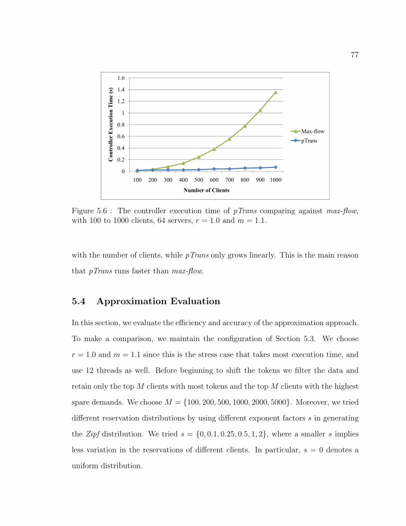
77

0.8

1

1.2

1.4

1.6

Con

trol

ler

Exe

cuti

on T

ime

(s)

0

0.2

0.4

0.6

0.8

100 200 300 400 500 600 700 800 900 1000

Con

trol

ler

Exe

cuti

on T

ime

(s)

Number of Clients

Max-flow

pTrans

Figure 5.6 : The controller execution time of pTrans comparing against max-flow,with 100 to 1000 clients, 64 servers, r = 1.0 and m = 1.1.

with the number of clients, while pTrans only grows linearly. This is the main reason

that pTrans runs faster than max-flow.

5.4 Approximation Evaluation

In this section, we evaluate the efficiency and accuracy of the approximation approach.

To make a comparison, we maintain the configuration of Section 5.3. We choose

r = 1.0 and m = 1.1 since this is the stress case that takes most execution time, and

use 12 threads as well. Before beginning to shift the tokens we filter the data and

retain only the top M clients with most tokens and the top M clients with the highest

spare demands. We choose M = 100, 200, 500, 1000, 2000, 5000. Moreover, we tried

different reservation distributions by using different exponent factors s in generating

the Zipf distribution. We tried s = 0, 0.1, 0.25, 0.5, 1, 2, where a smaller s implies

less variation in the reservations of different clients. In particular, s = 0 denotes a

uniform distribution.

78

60

80

100

120

Per

cent

age

of W

eak

Exc

ess

Tok

ens

Rem

oved

s = 0

s = 0.1

0

20

40

60

100 200 500 1000 2000 5000

Per

cent

age

of W

eak

Exc

ess

Tok

ens

Rem

oved

Number of Clients Considered for Top Demands and Spare Capacities

s = 0.1

s = 0.25

s = 0.5

s = 1

s = 2

(a) Percentage of weak excess tokens removed with different M .

0.08

0.1

0.12

0.14

0.16

Con

trol

ler

Exe

cuti

on T

ime

(s)

0

0.02

0.04

0.06

0.08

100 200 500 1000 2000 5000 10000

Con

trol

ler

Exe

cuti

on T

ime

(s)

Number of Clients Considered for Top Demands and Spare Capacities

(b) Execution time with 12 threads and different M .

Figure 5.7 : Error and execution time with approximation.

Recall that the goal of the shift steps is to reduce the number of weak excess

tokens. Figure 5.7a shows the percentage of weak excess tokens removed by using

different M and s. Form the figure, we can see that though there are 10000 clients,

considering only the top 2000 (20%) clients is enough to remove all the weak excess

tokens, even with the uniform reservation distribution. Moreover, we can still remove

79

more than 70% weak excess tokens using only the top 500 (5%) clients. One can

also see that for a fixed M we remove more weak excess tokens when the skew in

the reservation distribution increases, reaching 100% success with just 1− 5% of the

clients. Since skewed distributions are more likely in practice, the approximation will

be especially useful in these cases.

The benefit of the approximation approach is that it can further accelerate the

execution time of the pTrans algorithm. Figure 5.7b shows the running time of the

pTrans algorithm with different M . It can be seen that we can achieve another 5×

speedup on top of the parallelization approach while still keeping the accuracy at a

reasonable threshold.

5.5 Handling Demand Fluctuation

In our proposed QoS framework, the allocation of the tokens is based on the estimation

of the future demand based on the recent history of request arrivals at a server. In

this section, we therefore study how the framework adapts to demand fluctuations

which cause incorrect demand estimates. In this experiment, there are two clients A,

B with reservations 200 IOPS and unbounded limits, and two servers each capable of

200 IOPS. A is continuously backlogged on both servers and B alternates its demand

between the servers. Specifically, it sends 20 requests to one of the servers on alternate

100ms intervals, starting with server 1.

Based on their capacities, each server can do 20 requests in a 100ms interval. An

offline algorithm would observe that both reservations can be met by scheduling 20

requests of B on server 1 and 20 requests of A on server 2 in the first 100ms interval,

and then flipping the servers of A and B in the next 100ms interval, and so on. After

1 second both clients will receive their reservations of 200 IOPS.

80

(a) Initial token allocation constraints at time0.

(b) The token allocation constraints at time100ms.

(c) The token allocation constraints at time200ms.

(d) The token allocation constraints at time300ms.

(e) The token allocation constraints at time400ms.

(f) The token allocation constraints at time900ms.

Figure 5.8 : The token allocation constraints in the demand fluctuation experiment,with redistribution interval = 100ms.

81

However, an online algorithm that does not know of the arrival pattern can

wrongly estimate the demand causing an inaccurate distribution of tokens. The

pattern here is the worst-case for the demand estimation: it will always predict the

demand incorrectly in every interval. However, we show that we are still able to come

close to satisfying the reservations.

To better show the token allocation constraints, we show the token allocation

graph in the max-flow model proposed in Section 3.3.2. The initial token allocation

is shown in Figure 5.8a. Client A has its reservation divided equally between the

two servers, while client B does not allocate any tokens since its predicted demand,

based on its previous history, is zero. In the first 100ms interval, both A and B

have requests at server 1; however B has no reservation tokens while A has enough

reservation tokens to saturate the server. Hence A will get 20 requests at server 1

while B will not get any. B will have a pending queue of 20 requests which together

with the arrival of 20 requests will be projected to an estimated demand of 20+20×9

= 200 requests for the next allocation. Meanwhile, server 2 which only has requests

from A will complete 20 of its requests as well. Also since there are no pending

requests or arrivals for B on server 2, its estimated demand will be zero. The token

allocation at 100ms is shown in Figure 5.8b. Based on the predicted demand, the

controller moves all 180 tokens of B to server 1, and all 160 tokens of A to server 2.

The process repeats in every interval, and the pattern follows that of the offline

algorithm except that it is one interval behind, serving queued requests of B on the

server on which it has no current request arrivals (see Figures 5.8c - 5.8e). The final

token allocation is shown in Figure 5.8f at 900 ms, where client A has consumed all

its reservation tokens. As a result, A does 10 normal requests on server 2 while B

finishes 10 of its 20 reservation requests on server 1. Totally, A finishes 210 requests,

while B finishes 190 requests. Figure 5.9a shows the number of requests scheduled of

82

150

200

250

Nu

mb

er o

f R

equ

ests

Fin

ish

ed

0

50

100

0 1 2 3 4 5 6 7 8 9 10

Nu

mb

er o

f R

equ

ests

Fin

ish

ed

Time (*100ms)

Client A

Client B

(a) Redistribution interval = 100ms.

150

200

250

Nu

mb

er o

f R

equ

ests

Fin

ish

ed

0

50

100

0 0.5 1 1.5 2 2.5 3 3.5 4 4.5 5 5.5 6 6.5 7 7.5 8 8.5 9 9.5 10

Nu

mb

er o

f R

equ

ests

Fin

ish

ed

Time (*100ms)

Client A

Client B

(b) Redistribution interval = 50ms.

150

200

250

Nu

mb

er o

f R

equ

ests

Fin

ish

ed

0

50

100

0 2 4 6 8 10

Nu

mb

er o

f R

equ

ests

Fin

ish

ed

Time (*100ms)

Client A

Client B

(c) Redistribution interval = 200ms.

Figure 5.9 : Number of Requests vs Time with Demand Fluctuation.

83

both clients against time.

Next, we change the redistribution interval to 50ms, to see if redistributing more

frequently can handle the demand fluctuation better. Figure 5.9b shows the number

of requests scheduled for both clients, where we see that B’s reservation is still not

met. On the other hand, if we change the redistribution interval to 200ms, the

controller can handle the demand fluctuation better, since the interval is large enough

to absorb and accurately smooth out the rapid demand fluctuation of B. Figure 5.9c

shows the number of requests scheduled. We can see this time both clients meet their

reservations, since the controller has accurately estimated the demand.

5.6 Linux Evaluation

In this section, we describe results on the Linux cluster in three experiments. In

Section 5.6.1 we use a small configuration with static demands to show how pTrans

meets reservations and limits. We then consider dynamically varying demands in

Section 5.6.2. These experiments are done using Memcached as the backend server.

Finally, Section 5.6.3 shows the evaluation results using file I/O.

5.6.1 Memcached Evaluation with Static Demand

In this experiment, we show how pTrans handles reservations and limits with a sim-

ple and steady configuration of 4 clients and 4 servers. We initially focus on reser-

vations; each client has a reservation of 30, 000 RPS and an essentially unbounded

limit (200, 000 RPS was used in the experiment). Clients 1, 2, 3, 4 are continuously

backlogged on servers 1, 1, 2, 1, 2, 3 and 1, 2, 3, 4 respectively with 5 out-

standing requests. We choose a QoS period of 1 second. For the token allocation,

we redistribute tokens every 200ms i.e. we have 5 token redistributions in each QoS

84

period. Theoretically, if no QoS controls are applied, the round-robin scheduler will

give clients 1, 2, 3, 4 throughputs in the ratio of (1/4) : (1/4+1/3) : (1/4+1/3+1/2) :

(1/4 + 1/3 + 1/2 + 1) = 3 : 7 : 13 : 25, which results in average throughputs of 12500,

29166, 54166, and 104166 RPS, respectively. On the other hand, when QoS controls

are applied, the reservations of all clients are expected to be met.

Figures 5.10a and 5.10b show the results of the execution, which matches our

theoretical analysis. Figure 5.10a shows the throughput of the clients without QoS

controls and the results match the predicted throughputs closely. In Figure 5.10b the

throughputs with reservation controls are shown. Client 1’s throughput, which was

well below its reservation, now increases to match the required 30, 000 RPS. Looking

at Figure 5.10b we can see that client 4 reaches its reservation first (at roughly 400ms)

since it gets service on all servers. At that point it loses priority in scheduling and the

other clients get increased service; this can be seen most dramatically by the change

in the slope of client 1 at that time.

Finally, we set the limit of each client to be 60, 000 RPS. Figure 5.11 shows the

execution results. We can see that both reservations and limits are met by all the

clients. Figure 5.11 looks similar to Figure 5.10b in the interval 0 to 0.6s, where the

servers are basically doing reservation requests. Beyond this time client 4 gradually

slows down as it meets its limit threshold in each sub-interval, yielding to clients that

are further away from their limit.

5.6.2 Memcached Evaluation with Dynamic Demand

We now show how pTrans guarantees QoS on the cluster when demands change

dynamically. We use a larger configuration of 8 servers and 10 clients. Each client

has a reservation of 30, 000 RPS and a limit of 50, 000 RPS. Each client randomly

chooses a number between 2 to 6 active servers; at every demand change instant, a

85

60000

80000

100000

120000

Nu

m o

f R

equ

ests

Don

e

Client 1

0

20000

40000

60000

0 0.2 0.4 0.6 0.8 1

Nu

m o

f R

equ

ests

Don

e

Time (s)

Client 1

Client 2

Client 3

Client 4

(a) The number of requests being completed with simple round-robin scheduler.

50000

60000

70000

80000

90000

100000

Nu

m o

f R

equ

ests

Don

e

Client 1

0

10000

20000

30000

40000

50000

0 0.2 0.4 0.6 0.8 1

Nu

m o

f R

equ

ests

Don

e

Time (s)

Client 1

Client 2

Client 3

Client 4

(b) The number of requests being completed with pTrans scheduler with onlyreservations.

Figure 5.10 : The number of requests done for pTrans and simple round robin sched-ulers.

fresh set of active servers (between 2 and 6) is chosen. We allow 5 demand changes for

each client. We run 4 consecutive QoS periods with 5 redistributions in each period.

Figures 5.12a and 5.12b show the dynamic throughput for both scenarios. From

86

40000

50000

60000

70000

Nu

m o

f R

equ

ests

Don

e

Client 1

0

10000

20000

30000

0 0.2 0.4 0.6 0.8 1

Nu

m o

f R

equ

ests

Don

e

Time (s)

Client 1

Client 2

Client 3

Client 4

Figure 5.11 : The number of requests being completed with pTrans scheduler withreservations and limits.

the figures, we can see with the simple round-robin scheduler, the QoS is not guar-

anteed, as some clients (e.g. clients 5, 7 and 8) in QoS period 1 did not meet their

reservations, and some clients (e.g. clients 3 and 4) received throughput exceeding

their limits. In contrast, by using the pTrans scheduler, both reservation and limit

QoS was guaranteed in all intervals for all clients.

Finally, we tested a bigger problem size using 200 clients. On average without QoS

controls, 68.5% of the clients met their reservations and 83.5% did not go beyond their

limits. In contrast, when using pTrans, 99.6% of the clients met their reservations and

none exceeded their limits. By running the QoS controller for 15 minutes, we found

on average, the communication in every 1s QoS period takes 9ms, i.e. the average

communication overhead is around 0.9%.

87

40000

50000

60000

70000

Nu

m o

f R

equ

ests

Don

e Client 1

Client 2

Client 3

Client 4

0

10000

20000

30000

1 2 3 4

Nu

m o

f R

equ

ests

Don

e

QoS Period

Client 4

Client 5

Client 6

Client 7

Client 8

Client 9

Client 10

(a) The number of requests being completed with simple round-robin scheduler.

40000

50000

60000

70000

Nu

m o

f R

equ

ests

Don

e Client 1

Client 2

Client 3

Client 4

0

10000

20000

30000

1 2 3 4

Nu

m o

f R

equ

ests

Don

e

QoS Period

Client 4

Client 5

Client 6

Client 7

Client 8

Client 9

Client 10

(b) The number of requests being completed with pTrans scheduler.

Figure 5.12 : Total number of request completed for pTrans and simple round-robinscheduler.

5.6.3 File I/O Evaluation

Finally, we show how our storage prototype with pTrans guarantees reservation and

limit QoS when doing block file I/O. In this experiment, we have 8 servers and

88

200 clients, and 80% of the total server capacities are being reserved, i.e. r =

(∑

i∈BRi)/(∑

j∈SCj) = 0.8. The client reservations (shown in Figure 5.13) and

demands follow the same Zipf distribution that we used in the simulation, and each

client allows 2 demand changes in the QoS period as before. Here we also assign each

client a limit equal to 1.5 times its reservation.

500

600

700

800

900

1000

Res

erva

tion

s

0

100

200

300

400

500

1 9 17 25 33 41 49 57 65 73 81 89 97 105

113

121

129

137

145

153

161

169

177

185

193

Res

erva

tion

s

Client ID

Figure 5.13 : The Zipf distribution of clients’ reservation requirements in Linux QoSevaluation.

We set the QoS periods to be 5 seconds, and in each QoS period we do 5 token

allocations, i.e. each redistribution interval is 1 second. We run the server for two

QoS periods (i.e. 10 seconds) and record the QoS result as the number of requests

being completed in each redistribution interval. Servers continue to serve I/Os as the

controller is computing new token allocations.

Figure 5.14a and Figure 5.14b shows the number of requests being done in both

QoS periods. From the figures, we can see pTrans provides the reservation and limit

QoS in a reasonable manner. The needles, similar to those shown in the simulation,

89

indicate how pTrans handles demand changes. Quantitatively, only one client (0.5%)

missed its reservation by more than 1%, and no client exceeded its limit.

500

600

700

800

900

1000N

um

of

Req

ues

ts D

one

0

100

200

300

400

500

1 9 17 25 33 41 49 57 65 73 81 89 97 105

113

121

129

137

145

153

161

169

177

185

193

Nu

m o

f R

equ

ests

Don

e

Client ID

(a) The number of requests being completed in the first QoS period.

500

600

700

800

900

1000

Nu

m o

f R

equ

ests

Don

e

0

100

200

300

400

500

1 9 17 25 33 41 49 57 65 73 81 89 97 105

113

121

129

137

145

153

161

169

177

185

193

Nu

m o

f R

equ

ests

Don

e

Client ID

(b) The number of requests being completed in the second QoS period.

Figure 5.14 : The the number of requests being completed in Linux QoS evaluation.

90

Chapter 6

Response Time QoS

6.1 Chapter Overview

In this chapter, we introduce Fair-EDF, a framework for providing fairness to clients

in a shared storage server, while guaranteeing their latencies. Fair-EDF aims to

schedule requests to meet their specified deadlines. When it detects that the server

is overloaded, it drops some requests so that the remaining requests can meet their

deadlines. Fair-EDF drops the minimum number of requests while trying to balance

this penalty among the clients.

Fair-EDF uses the earliest deadline first (EDF) [61] scheduling policy at the back-

end, while adding a front-end controller that selects and drops requests in the schedul-

ing queue when it detects that latency violations will occur. It extends the idea of

the offline RT-OPT [62] framework to work in an online situation and adds fairness.

Fair-EDF assumes an OS such as MittOS [41] is already in place which provides sys-

tem support for dropped requests. In practice, Fair-EDF would be especially useful

in streaming applications, such as streaming video from object storage.

6.2 Problem Statement

In this section, we present the latency fairness QoS problem. We focus on a single

server for developing our Fair-EDF algorithm. In a distributed cluster, we propose a

solution where QoS enforcement is done independently by each server; periodically,

91

the servers coordinate to adjust the QoS targets to satisfy the global fairness require-

ments. In this thesis, we concentrate on the latency QoS algorithm at each server.

The coordination of QoS controls between servers will be studied in future work.

The storage server is shared by a number of clients that send I/O requests to

the server. Each request has a stipulated latency (response time) bound. Large I/O

operations are assumed to be chunked into fixed-size I/O requests. The service time of

all requests is upper-bounded by σ. The service time is the interval between the time

the request is dispatched to the storage device and its completion time. A request

must complete its execution in σ time after being scheduled; else it is assumed to

time-out and abort. A request r that arrives at time tr is assigned a deadline dr equal

to the sum of its arrival time and latency bound. A request is said to be successful if

it completes execution before its deadline, and missed otherwise i.e. if it was dropped

(not scheduled), or scheduled but aborted after σ time. Each request can have its

own latency bound dr− tr based on some classification. On the other hand, a client i

can also choose to specify a single latency bound δi for all its requests, which implies

that dr = tr +δi. However, this situation is covered by the more general specification.

Finally, we require that the latency bound is at least the service time bound σ; i.e.

tr + σ ≤ dr is always true.

Furthermore, we define the client success ratio, si, as the fraction of client i’s

requests that succeed. The system success ratio S is the fraction of the total number

of requests that succeed. The goal of our framework is to shape the si subject to

maximizing S. In this thesis, we let each client i specify its required success ratio qi as

its SLO, and the algorithm will try to ensure each client i has si ≥ qi. In our model, a

client can specify any success ratio, but in practice, the success ratios would shadow

the priorities of the clients. For example, premium clients with higher priorities are

able to specify higher required success ratios.

92

Example 6.2.1. We motivate the latency fairness framework with the following

example. Suppose a server of 100 IOPS capacity is shared by two clients A and B,

which send uniformly-sized I/O requests with a service time of 10ms each. At time 0,

A sends a burst of 100 requests with deadlines all at 1s. Client B sends I/O requests

at a uniform rate every 10ms apart and all request have a latency bound of 40ms, i.e.

B sends requests at times 0, 10, 20, ..., with deadlines of 40, 50, 60, ... respectively.

Almost all of the 200 requests arriving at the server in one second have deadlines

of 1 second or less. Meeting these deadlines would require at least double the server

IOPS capacity. An EDF [61] scheduler, which is commonly used for supporting

latency requirements, will do almost all of B’s requests first, followed by those of A.

Most requests of B will meet their deadlines and almost no requests of A will do so,

resulting in poor fairness. Furthermore, all new requests arriving in the next second

will also miss their deadlines.

6.3 Basic Fair-EDF Framework

In this section, we describe our basic Fair-EDF framework. Figure 6.1 shows the

components of the framework. When any request arrives at the server, the request is

tentatively accepted for scheduling by adding it to a taken queue. If service demands of

the requests in the taken queue exceed the system capacity, then one or more pending

requests needs to be dropped. Requests in the taken queue wait for their turn to be

dispatched by the scheduler; during its wait, the request may still be dropped as new

requests arrive. The system provides fairness by selecting requests to drop so that

each client meets its latency SLO. The Fair-EDF controller decides when to discard a

request and which request to drop based on the QoS requirements. Different fairness

criteria can be substituted in the controller without changing the framework.

93

A standard EDF scheduler is used to dispatch requests in deadline order. All

requests that remain in the taken queue are guaranteed to meet their deadlines even

in the worst case. The Fair-EDF controller extends the idea of the offline RT-OPT [62]

framework to work in an online situation and add fairness.

Taken Queuerequests

from clients

overloaded requestsget dropped

EDF scheduling(deadlines guaranteed)

Fair-EDFController

Standard EDFScheduler

Figure 6.1 : The basic Fair-EDF framework.

6.4 Fair-EDF Controller

The Fair-EDF Controller determines whether a new request is added to the taken

queue or gets dropped. If it is added to the taken queue, an existing request may

sometimes be dropped in order to guarantee that all deadlines in the taken queue can

be met.

6.4.1 Occupancy Chart

We first discuss the idea behind the algorithm followed by some implementation

details. Let σ denote an upper bound on the service time of a request r and dr

denote its deadline. The current set of accepted requests are conceptually placed on

a timeline called an occupancy chart. Request r occupies the interval [tr, tr + σ] on

the timeline where tr is the latest time it can begin execution while ensuring that it

94

and all requests with deadlines later than dr are successful. The occupancy chart is

naturally partitioned into alternating busy and idle segments; a busy segment consists

of a continuous sequence of intervals while an idle segment is not covered by any

interval. As long as no interval crosses the current time Tnow, all requests will meet

their deadlines when scheduled in EDF order.

Example 6.4.1. Consider two clients A and B. Each request has a worst-case service

time of σ = 10ms. Client A has 4 requests a1, a2, a3, a4 with deadlines 30, 100, 100,

and 140ms respectively, and Client B has 3 requests b1, b2, b3 with deadlines 50, 145

and 150ms. Suppose the current time is 10ms. Figure 6.2a shows the occupancy

chart. Request b3 occupies the interval [140, 150]; b2 cannot be scheduled at 135 as it

would conflict with b3, and occupies the interval [130, 140]. Similarly a4 must occupy

the interval [120, 130], resulting in the busy segment [120, 150] comprising requests

a4, b2, b3. In the same way a2, a3 comprises busy segment [80, 100], a1 forms

segment [20, 30], and b1 forms segment [40, 50].

In the implementation, we do not keep track of the interval for each request in the

occupancy chart. Instead, we maintain the current busy segments in the occupancy

chart, and for each request, we keep track of the busy segment it belongs to. In

particular, we use S1, S2, · · ·Sn to denote the current set of busy segments and let Si

span the time range [Li, Ri]. We also let Sn+1 = [∞, ∞] as a sentinel. Since we

employ a standard EDF scheduler for the backend, requests in each busy segment are

implicitly organized by the EDF order.

Example 6.4.2. We use the same setup of Example 6.4.1 in Figure 6.2a. For the

occupancy chart, we maintain 4 busy segments: S1 = a1, [L1, R1] = [20, 30];

S2 = b1, [L2, R2] = [40, 50]; S3 = a2, a3, [L3, R3] = [80, 100]; S4 = a4, b2, b3,

[L4, R4] = [120, 150]. Within a segment the requests are arranged in EDF order as

95

b310 20 30 40 50 80 100 120 150

b1 a4a3a1 b2a290 130 140

(a) The initial occupancy chart in Examples 6.4.1 and 6.4.2.

b310 20 30 40 50 80 100 120 150

b1 a4a3a1 b2a290 130 140

a560 70

(b) The occupancy chart in Example 6.4.3 after accepting a5.

b310 20 30 40 50 80 100 120 150

b1 a4a3a1 b2a290 130 140

b460 70

a5

(c) The occupancy chart in Example 6.4.3 after accepting b4.

b310 20 30 40 50 80 100 120 150

b1 a4a3a1 b2a290 130 140

b460 70

a5c1

(d) The occupancy chart in Example 6.4.4 after accepting c1.

b310 20 30 40 50 80 100 120 150

b1 a4a3a1 b2a290 130 140

b460 70

a5c1 c20

(e) The occupancy chart in Example 6.4.4 after accepting c2.

b310 20 30 40 50 80 100 120 150

b1 a4a3 b2a290 130 140

b460 70

a5c1 c2

(f) The occupancy chart in Example 6.4.5 after dropping a1.

Figure 6.2 : An illustration of the occupancy chart in Examples 6.4.1, 6.4.2, 6.4.3, 6.4.4and 6.4.5.

96

shown in Figure 6.2a. For instance, by organizing the requests in S4 = a4, b2, b3 in

EDF order in the busy interval [L4, R4] = [120, 150], they will occupy the intervals

[120, 130], [130, 140] and [140, 150], respectively.

It has been proved that for a set of independent jobs with arbitrary release times

and deadlines, the standard EDF scheduler will always find a feasible∗ schedule if and

only if there exists one [63, 64]. Therefore, as long as we can ensure there exists a

feasible schedule for the requests in the occupancy chart, then by scheduling them

using the standard EDF scheduler, the deadlines of those requests can be guaranteed.

6.4.2 Handling New Requests

When a new request r arrives, we must identify the busy segment containing its

deadline, followed by updating the boundaries for the segment. This may now cause

some segments to overlap, leading to a cascade of boundary changes and segment

merges. If the start time of the earliest (leftmost) segment (i.e. L1) is smaller than

the current time Tnow, then the current set of requests in the taken queue cannot all

meet their deadlines, and one or more will need to be dropped so that the rest can

be successful.

Let dr denote the deadline of the new request r:

Case 1: dr lies between two consecutive segments Sk and Sk+1 i.e. Rk < dr < Lk+1.

Request r is assigned the interval [dr − σ, dr]. If dr − σ > Rk then we create a new

segment [dr − σ, dr] for r that lies between Sk and Sk+1. Otherwise, r is assigned

to Sk by merging the interval [dr − σ, dr] with the segment Sk: Lk is reduced by

σ − (dr − Rk) (the amount of overlap) and Rk is changed to dr. Note that changing

∗Given a set of requests, a schedule is feasible if it meets all deadlines of the requests.

97

Lk may cause Sk to overlap segment Sk−1, potentially causing a cascade of merges of

adjacent segments.

Case 2: dr lies within a segment Sk i.e. Lk ≤ dr ≤ Rk. In this case, r is assigned to

segment Sk and Lk is reduced by σ. Once again, reducing Lk may cause segments Sk

and Sk−1 to overlap, potentially triggering a cascade of merges of adjacent segments.

In general, when a request arrives it is placed on the timeline using case 1 or 2

above. If the first segment now begins at a time less than the current time (this

can happen only if the left boundary of the first segment S1 changes), we say the

occupancy chart is overloaded, and some request in S1 has to be dropped.

Example 6.4.3. Continuing Example 6.4.1, suppose there is a new request a5 with

deadline 70ms. The request’s deadline 70 falls between two segments [40, 50] and

[80, 90] (i.e. Case 1), and it can be assigned as the new segment [60, 70], since it

will not conflict with existing requests (see Figure 6.2b). Next a new request b4 with

deadline 45ms arrives. Since its deadline 45 falls inside the second segment [40, 50]

(i.e. Case 2), it will be assigned to the second segment, and will be assigned the

interval [30, 40]. Now the two adjacent segments [20, 30] and [40, 50] will merge into

a single segment [20, 50], as shown in Figure 6.2c.

Example 6.4.4. In Figure 6.2c, suppose two new requests c1 and c2 from client C,

with deadlines 25 and 40, arrive at time 10. From Case 2 above, c1 will be assigned to

the first segment and occupy the interval [10, 20] (see Figure 6.2d). Since the current

time is 10, this is a feasible schedule in which all requests will meet their deadlines

if they are executed in EDF order. Next c2 will be assigned to the first segment as

well. Now the first segment S1 spans the interval [0, 50], which contains requests

c1, a1, c2, b4 and b1, with deadlines 25, 30, 40, 45 and 50, respectively. These will

98

occupy the intervals [0, 10], [10, 20], [20, 30], [30, 40] and [40, 50], respectively (see

Figure 6.2e). Now the first segment S1 starts at time 0, which is smaller than the

current time 10, which means the occupancy chart now become overloaded.

Example 6.4.5. Continuing Example 6.4.4, we must drop one request to create a

feasible schedule. A set of candidate requests is c1, a1, b4, c2. The choice of which of

these requests to drop is governed by the QoS policy. Among the candidate requests

for dropping, we will drop a request from the client i with maximum si/qi value, i.e.

the client that has the highest current fulfillment ratio. Say we dropped a1, then the

resulting occupancy chart becomes in Figure 6.2f which is no longer overloaded.

Algorithm 10 shows the pseudo-code of the Fair-EDF controller algorithm. In

Section 6.4.3, we formally describe the set of candidate requests which can be dropped

when there is a server overflow, and give a proof of the correctness of the algorithm.

We also prove that this is a sufficient condition to ensure that the removal of any

such request will result in a feasible schedule. We leave as an open question for future

work the derivation of the necessary and sufficient conditions for a request to be a

candidate for dropping, and efficient implementations of the same.

6.4.3 Candidate Set Identification

Consider a snapshot of the first segment of the occupancy chart at time t0. For

notational convenience, we normalize the chart so that each interval is of length 1

(rather than σ), and denote the first segment by Σ.

Let there be n requests r1, r2, · · · rn at time t0 arranged in deadline order; that is

if di denotes the deadline of ri then d1 ≤ d2 ≤ d3 · · · ≤ dn. Without loss of generality,

let r1 occupy the interval (slot) [s, s + 1] in Σ; since all the slots in Σ are occupied

with no gaps, request ri occupies the slot [s+ i− 1, s+ i].

99

Algorithm 10: Fair-EDF Controller Algorithm

// A new request r with deadline dr arrives

// Adjusting the occupancy chart according to Tnowwhile R1 ≤ Tnow do

Remove S1 and re-number segments;

if L1 < Tnow thenL1 = Tnow;

// Adding r to the occupancy chartAdd r to the taken queue;Find Sk, where Rk < dr < Lk+1 or Lk ≤ dr ≤ Rk;if Rk < dr < Lk+1 then

// Case 1Create and insert new segment S ′k = [dr − σ, dr] between Sk and Sk+1;Assign r to S ′k;k = k′;

else// Case 2Lk = Lk − σ;Assign r to Sk;

// Merging the overlapping segmentswhile k > 1 and Rk−1 ≥ Lk do

Lk−1 = Lk−1 − (Lk −Rk−1);Rk−1 = Rk;Remove Sk;k = k − 1;

// Handling request overloadingif L1 < Tnow then

Let i be the client with the highest si/qi value that has a request r ∈ C,where C is defined in Section 6.4.3;

// Note: r may be same as r. In basic Fair-EDF (Section 6.3), ris discarded and marked as missed. With best-effort scheduling(Section 6.5), r is put into the dropped queue.

Drop r;L1 = L1 + σ;

100

Observation 6.1: If ri is scheduled no later than s+ i− 1 (that is the left-endpoint

of the interval it occupies) it will meet its deadline.

Observation 6.2: Σ has a feasible schedule in which all requests can meet their

deadline, if and only if if s ≥ t0.

Suppose Σ has a feasible schedule. Now a new request r∗ with deadline dr∗ is

inserted into Σ, and assume that dk ≤ dr∗ < dk+1. Σ is modified to a segment Σ∗

for the (n + 1)-request sequence: r1 · · · rk, r∗, rk+1, · · · rn. Each request ri, 1 ≤ i ≤ k,

is shifted one slot to the left and occupies the slot [s + i − 2, s + i − 1] in Σ∗. The

requests ri, k + 1 ≤ i ≤ n, occupy the same slots as they did in Σ, and r∗ occupies

the slot [s+ k − 1, s+ k].

If Σ∗ does not have a feasible schedule the controller needs to discard one of the

requests to ensure a feasible schedule. We need to identify as many requests that can

be discarded while guaranteeing that the remaining requests have a feasible schedule.

We call the set of requests that can be discarded as the candidate set. A larger

candidate set implies a larger pool from which to select a victim.

Some obvious possibilities for candidate requests are readily apparent. Discarding

the new request r∗ will allow Σ∗ to revert to the feasible schedule of Σ; similarly,

discarding the request occupying the first slot [s− 1, s] where t0 < s, will also solve

the problem. To completely characterize the candidate set we introduce the following

definitions.

Definition 6.1: Define the slack of a request in Σ∗ as the amount of time it can

be delayed while still meeting its deadline. If a request with slack ρ ≥ 1 currently

occupies slot [u, u + 1] then it will still meets its deadline if scheduled in any of the

later slots [u+ 1, u+ 2], [u+ 2, u+ 3] · · · [u+ ρ, u+ ρ+ 1].

Definition 6.2: Define λ to be the largest integer such that s+ λ ≤ dr∗ , where dr∗ is

the deadline of the new request r∗.

101

Note that r∗ occupies slot [s+ k − 1, s+ k] in Σ∗. If λ = k then r∗ occupies slot

[s+ λ− 1, s+ λ].

Lemma 12. If λ− 1 ≥ k+ 1, all requests rk+1, rk+2, · · · , rλ−1 have a slack of at least

1 in Σ∗.

Proof. A request ri, k + 1 ≤ i ≤ λ − 1, has a deadline di > dr∗ ≥ (s + λ).

Hence it can meet its deadlines if it is scheduled in the slot [s+ λ− 1, s+ λ]. Since

rλ−1 currently occupies slot [s + λ− 2, s + λ− 1], it has a slack of 1. All remaining

ri, k + 1 ≤ i < λ− 1, have slack greater than 1.

Corollary 12.1. If λ− 1 ≥ k, request r∗ has a slack of 1 in Σ∗.

Lemma 13. All requests r1, r2, · · · , rk have a slack at least 1 in Σ∗.

Proof. Any request ri, 1 ≤ i ≤ k that occupies a slot [u, u+ 1] in Σ, will occupy the

slot [u − 1, u] in Σ∗. Since Σ had a feasible schedule, ri must have a slack of 0 or

higher in Σ, and hence a slack of 1 or more in Σ∗.

Theorem 14. Let C = ri, i = 1 · · ·λ∪r∗. Then if any request r ∈ C is dropped,

the remaining requests have a feasible schedule.

Proof. Whichever request from C is dropped, the remaining requests have a slack of

at least 1. Hence all requests occupying slots earlier than that of the dropped request

can be moved forward by one slot, and no request will required to be scheduled before

t0.

6.5 Fair-EDF Scheduler for Best-Effort Scheduling

Since in practice, the upper bound on service time, σ, overestimates the actual ser-

vice time, the basic Fair-EDF may unnecessarily drop some requests because of the

102

pessimistic assumption. Therefore, we are motivated to add a second-chance policy

to the basic scheme. In this approach, the requests dropped from the taken queue

are not discarded immediately but queued and executed opportunistically if there

is free bandwidth before their deadlines. We therefore add a best-effort scheduling

component to Fair-EDF. The new framework is shown in Figure 6.3, where a dropped

queue is added. Similar to the taken queue, the dropped queue is also a priority queue

based on request deadlines, and all dropped requests are moved to the dropped queue

for best-effort scheduling.

Accordingly, instead of having the standard EDF scheduler in Figure 6.1, we

introduce our Fair-EDF scheduler. It keeps fetching and scheduling requests from

the taken queue and dropped queue. Requests in the taken queue are guaranteed to

meet their deadlines if their actual service times do not exceed σ. The dropped queue

is used for best-effort scheduling through work-stealing.

Taken Queuerequests

from clients

overloaded requestsget dropped

best effort scheduling(work stealing)

EDF scheduling(deadlines guaranteed)

Dropped Queue

Fair-EDFController

Fair-EDFScheduler

Figure 6.3 : The Fair-EDF framework with best-effort scheduling.

The request scheduling process is as follows: the Fair-EDF scheduler first removes

the requests in the dropped queue whose deadlines can no longer be guaranteed even if

they are scheduled immediately i.e. it removes all requests r for which Tnow +σ > dr.

These removed requests will be counted as missed. Now let tq and dq to be the requests

with earliest deadlines in the taken queue and dropped queue respectively. Fair-EDF

scheduler will perform work-stealing for dq if it can guarantee that scheduling dq will

103

not disrupt the guaranteed deadlines of requests in the taken queue, i.e. Tnow+σ ≤ ddq

and Tnow+σ ≤ L1 where L1 is the left boundary of the first segment of the occupancy

chart defined in Section 6.4.1. If work-stealing cannot be performed, the scheduler

will schedule tq instead. If the first of the conditions is violated the request dq is

discarded and marked as missed. The opportunity for work-stealing arises because

not all requests will use their worst-case allocated service time, and the excess is

returned to the system as credit; when the total credit reaches σ, we will have the

chance to schedule requests from the dropped queue.

Algorithm 11 shows the pseudo-code of the Fair-EDF scheduler algorithm for

best-effort scheduling.

6.6 Chapter Summary

In this chapter, we presented Fair-EDF, a framework providing fairness QoS for la-

tency guarantees in shared storage systems. Fair-EDF combines the idea of the offline

algorithm RT-OPT with the EDF scheduler, and employs a work-stealing mechanism

for best-effort scheduling. In the next chapter, we will show in the evaluation that

Fair-EDF gives reasonable fairness control with different runtime workload behaviors,

and the runtime overhead is relatively small.

104

Algorithm 11: Fair-EDF Scheduler Algorithm for Best-EffortScheduling

while TRUE do// Removing requests in the dropped queue with deadlinescannot be guaranteed

while DroppedQueue is not empty dodq = DroppedQueue.top();if Tnow + σ > ddq then

dq = DroppedQueue.pop();count dq as missed;

elsebreak;

L1 = the left boundary of the first segment of the occupancy chart;if DroppedQueue is not empty and Tnow + σ ≤ L1 then

// Work-stealingdq = DroppedQueue.pop();Schedule dq;if dq finishes within its deadline then

count dq as successful;else

count dq as missed;

elseif TakenQueue is not empty then

// Normal schedulingtq = TakenQueue.pop();Schedule tq;if tq finishes within its deadline then

count tq as successful;else

count tq as missed;

105

Chapter 7

Evaluation of Response Time QoS

7.1 Experimental Setup

In the evaluation, we compare Fair-EDF with a standard EDF scheduler, as well

as a variant of EDF we call Prudent-EDF. The problem with standard EDF is that

a capacity overload will cause the deadlines of future requests, those following the

overloaded period, to be missed as well. By contrast, Prudent-EDF drops requests

that it recognizes will miss their deadline, thereby preventing them from affecting

future request deadlines. Prudent-EDF drops a request at the latest possible time

and consequently, like an immediate-drop policy, cannot shape the QoS profile by

selecting an appropriate victim request to discard. However, like Fair-EDF, it will

drop the minimal number of requests in the worst case.

We implemented a prototype of the Fair-EDF framework in OpenMP. We use

different threads to handle the request controller and request scheduler and keep

them pinned on different cores. The arrival pattern and deadlines of the clients

are explicitly specified using external input files. The controller generates requests

at desired times. With Prudent-EDF, the scheduler chooses requests in deadline

order but will discard the request at the head of the queue if its deadline cannot

be guaranteed. For Fair-EDF, the controller maintains taken and dropped queues

as discussed in Section 6.5. The scheduler chooses a request from one of the queues

depending on whether it can perform work stealing or not and discards requests from

the head of the dropped queue that cannot be guaranteed.

106

The workload in our evaluation consists of random 4KB direct reads from a

1GB file. We run our experiments on a standard Linux server. The server node

is equipped with an Intel R© SSD DC S3700 hard disk [65] and an Intel R© Xeon R©

E5-2697 CPU [66]. We profiled the service time using the standard EDF scheduler

and a closed loop client which keeps the server always busy. The average profiled

service time for each request is 142µs, i.e. the server has an average throughput of

around 7050 IOPS.

7.2 Linux Evaluation

7.2.1 QoS Evaluation

In this evaluation, we have 2 clients. Client 1 sends one request every 0.15ms, with

a latency bound of 0.5ms. Client 2 sends a burst of 10 requests every 10ms, with a

latency bound of 25ms for each request. Client 1 has a request rate of 6667 IOPS,

and Client 2 a rate of 1000 IOPS. The load on the server is 7667 IOPS which exceeds

its capacity of 7050 IOPS. The specified success ratios for clients 1 and 2 are 0.9 and

0.8, respectively.

We ran the system for a second, and Figure 7.1 shows the success ratio of both

clients using the three policies. Figure 7.2a and 7.2b show the average response time

for both clients. We can see that EDF gradually misses the deadlines of both clients,

and the response times start to increase. Due to the chain effect of missed deadlines

for simple EDF scheduling under overload, it results in a poor success ratio for both

clients. For Prudent-EDF, technically no deadlines will be missed (since they are

proactively dropped). However, for this workload it keeps doing requests of client 1

and drops most of the requests of bursty client 2, resulting in poor fairness between

clients. Finally, Fair-EDF also guarantees that no deadlines will be missed and will

107

drop the same (minimal) number of requests as Prudent-EDF. However, it tries to

fairly distribute the pain of dropped requests according to the required success ratios.

0

0.1

0.2

0.3

0.4

0.5

0.6

0.7

0.8

0.9

1

1.1

1.2

0

50

10

0

15

0

200

25

0

300

35

0

40

0

450

50

0

55

0

60

0

65

0

700

75

0

80

0

850

90

0

950

Su

cces

s R

ati

o

Time (ms)

Client 1 (EDF)

Client 2 (EDF)

Client 1 (Prudent-EDF)

Client 2 (Prudent-EDF)

Client 1 (Fair-EDF)

Client 2 (Fair-EDF)

Figure 7.1 : The success ratio of both clients using three policies.

7.2.2 Effect of Overestimated Service Time

In practice, the actual service time is not fixed and the exact value may be unknown.

The σ we choose must be a strict upper bound of the service time and so we must

use an overestimate. To avoid losing throughput due to the conservative assumption

we use the dropped queue to pick up overflowing requests based on the estimated

service time. In this evaluation, we show how Fair-EDF handles overestimated σ,

especially how the dropped queue is used for utilizing the time credits caused by the

overestimation. We keep the same arrival pattern of the clients as Experiment 1.

However, we vary σ from 2× to 20× of the profiled average cost of 142µs. We set

the latency bound to be 10ms for both clients’ requests, which is greater than the

maximum service time as required (see Section 6.2).

108

0

5

10

15

20

25

30

35

40

0

50

100

15

0

20

0

25

0

300

35

0

40

0

450

50

0

55

0

60

0

650

70

0

75

0

800

85

0

90

0

95

0

Av

era

ge

Res

po

nse

Tim

e (m

s)

Time (ms)

Client 1 (EDF)

Client 1 (Prudent-EDF)

Client 1 (Fair-EDF)

(a) The average response time for Client 1 using three policies.

0

10

20

30

40

50

60

70

0

50

100

15

0

20

0

250

300

35

0

40

0

450

50

0

55

0

600

65

0

70

0

75

0

800

85

0

90

0

950

Av

era

ge

Res

po

nse

Tim

e (m

s)

Time (ms)

Client 2 (EDF)

Client 2 (Prudent-EDF)

Client 2 (Fair-EDF)

(b) The average response time for Client 2 using three policies.

Figure 7.2 : The average response time for both clients using three policies.

We run Fair-EDF for one second with different σ, and use Prudent-EDF as a

comparison. The success ratios are shown in Figure 7.3. From the figure, we can see

the system success ratio (green bar) does not decrease with the overestimation factor.

109

The reason is that with a higher σ, although fewer requests are placed in the taken

queue, each request finishes much earlier than σ and provides greater opportunities for

work-stealing in the dropped queue. Similarly, until σ gets very high (overestimate

by 10× the real cost), the QoS result is also good. With a high value of σ, the

fairness starts getting worse and approaches that of Prudent-EDF. The reason is that

with a high σ, many more requests are put into the dropped queue, making the

controller unable to catch up the changes. In the extreme case, with σ tending the

∞, all requests are put into the dropped queue, and the scheduler essentially becomes

Prudent-EDF. The experiment illustrates this predicted behavior.

0

0.1

0.2

0.3

0.4

0.5

0.6

0.7

0.8

0.9

1

1.1

1 2 4 6 8 10 12 14 16 18 20 Prudent

EDF

Su

cces

s R

ati

o

Times of Overestimation

Client 1

Client 2

System

Figure 7.3 : Evaluation result for different overestimated service times.

7.2.3 QoS Result for More Clients

In this evaluation, we have 10 clients sharing the server. The arrival patterns and

deadline specifications are shown in Table 7.1. Clients 1 to 8 send requests at different

fixed rates, and clients 9 and 10 are very bursty. The total load is again 7750 IOPS

exceeding the server capacity of 7050 IOPS.

110

ClientInter-ArrivalTime (ms)

BurstSize

Demand(IOPS)

DeadlineTime (ms)

1 0.4 1 2500 0.52 1 1 1000 13 1 1 1000 14 2 1 500 25 2 1 500 26 2 1 500 27 2 1 500 48 4 1 250 49 40 20 500 4010 50 25 500 50

Table 7.1 : The arrival pattern and deadline specifications of the clients.

For Fair-EDF, we introduce a grouping policy consisting of two groups: gold and

silver. The gold group has a required success ratio of 0.9, and the silver group has a

required success ratio of 0.8. We show the results of two grouping policies. Policy 1

groups clients 1 to 8 as gold and the rest as silver, and policy 2 does the opposite,

i.e. grouping clients 1 to 8 as silver and the rest as gold.

0

0.1

0.2

0.3

0.4

0.5

0.6

0.7

0.8

0.9

1

1.1

EDF Prudent-EDF Fair-EDF (Grouping Policy 1) Fair-EDF (Grouping Policy 2)

Su

cces

s R

ati

o

Client 1

Client 2

Client 3

Client 4

Client 5

Client 6

Client 7

Client 8

Client 9

Client 10

System

Figure 7.4 : Evaluation result for the experiment with ten-clients and two-groups.

111

We run the three schedulers for one second, and the success ratio for all clients as

well as the system is shown in Figure 7.4. From the figure, we can see that EDF has

poor success ratios for all clients since it gradually misses all deadlines if the capacity

is not enough. Both Prudent-EDF and Fair-EDF have a good system success ratio.

However, in Prudent-EDF, most requests of bursty clients 9 and 10 are dropped,

making their success ratios below the other clients and the system’s ratio. In contrast,

by using Fair-EDF, the success ratios of clients 9 and 10 go up to the required success

ratio of the group, while the success ratios of other clients do not decrease significantly,

resulting in better fairness. Moreover, Fair-EDF achieves a similar system throughput

as Prudent-EDF. This indicates Fair-EDF does not introduce much runtime overhead

compared with Prudent-EDF.

112

Chapter 8

Conclusions and Open Problems

8.1 Conclusions

In this thesis, we studied the problem of providing QoS in distributed storage systems,

and developed novel algorithms for providing bandwidth and latency guarantees. For

bandwidth allocation, we proposed bQueue, a novel coarse-grained scheduling frame-

work for reservation and limit QoS controls in distributed storage systems. bQueue

uses token allocation to control the number of high-priority reservation requests, and

to cap the maximum number of requests served for each client. To accommodate de-

mand and server capacity variations due to workload changes, token allocations are

recomputed at fixed intervals using dynamic demand and capacity estimates. Opti-

mization problem formulations based on Integer Linear Programming and Maximum

Network Flow were developed for token allocation. A simple token-sensitive round-

robin scheduler that executes at each server was developed to enforce the reservation

and limit requirements. Compared to fine-grained QoS solutions, bQueue does not in-

cur the extra overhead of using a centralized metadata server for tagging all requests

of a client, and uses a simple round-robin scheduler at the servers. Our performance

results show thatbQueue is able to handle run-time variations in demands and service

rates, and provide reasonable and accurate QoS to the clients.

We developed pTrans, a fast and scalable algorithm for solving the token allocation

problem. pTrans models the problem as distributing tokens on a small graph (number

of vertices equal to the number of servers) augmented with per-edge vectors reflecting

113

current client token allocations. pTrans greedily transfers tokens from overloaded to

underloaded servers while avoiding the creation of wasteful strong-excess tokens that

cannot be consumed due to insufficient demand. We formally proved that pTrans

converges to the global optimal in a polynomial number of steps. Furthermore, it has a

much smaller run time than existing approaches, and can be further accelerated using

parallelization. Empirical performance results show that pTrans achieves orders-of-

magnitude improvement in execution time over the alternative ILP and max-flow

based approaches.

For response time QoS we introduce Fair-EDF, a framework providing fairness

in latency tail distributions of concurrent clients. Fair-EDF combines the idea of

the offline algorithm RT-OPT with the standard EDF scheduler to identify overload

conditions at a server. It uses a data structure called occupancy chart for identifying

candidate requests that can be dropped to alleviate the overload. Fair-EDF also

incorporates a work-stealing mechanism for best-effort scheduling of dropped requests.

The evaluation results show that Fair-EDF is effective in meeting QoS guarantees for

different dynamic workload behaviors.

8.2 Open Problems

In this section, we discuss some open problems identified in the course of this research.

8.2.1 Bandwidth Allocation QoS

Demand and Capacity Estimation: In many practical situations, the demand

of the clients may not change too frequently. In such cases, recomputing token allo-

cations in fixed redistribution intervals may be unnecessary. Instead, we can use a

dynamic window to monitor the demand changes, and trigger token allocation only

114

if demands change beyond a threshold. A similar approach can be applied for server

capacity estimation. By using dynamic estimation, we can reduce the communication

overhead as well.

Additional QoS Controls: A broad open problem is how to provide QoS controls

such as weight-proportional bandwidth allocation in a distributed environment. We

will also study the token allocation problem for distributed systems which employ

data replication. In one such model, any server can be used to satisfy a read request,

leading to additional choices in the token distributions. Dealing with writes in this

environment creates additional challenges and depends heavily on the write protocols

and consistency models in place.

Distributed Token Controller: In the current design, the token controller is cen-

tralized. An open problem is to investigate ways to distribute the token control

algorithm to further improve the scalability.

8.2.2 Response Time QoS

In this section, we discuss some open issues and challenges for Fair-EDF.

Average service time estimation: Estimating the service time of a request once

it is dispatched to the back-end server is a challenging problem. By improving the

estimated upper-bound, Fair-EDF can reduce the number of requests that need to be

served on a best-effort basis, and thereby increase the fairness of the tail latency dis-

tributions. This is an orthogonal issue to our results. MittOS [41] studied predicting

the request costs for better handling requests latencies.

Variable request service times: A difficult problem is to adapt Fair-EDF to

efficiently support requests with highly variable service times, so a single upper-bound

σ is unreasonable. The current algorithm will need to be generalized to handle this

115

situation. For instance, in the substitution, one long request may cause several short

requests to be dropped, and a single substitution may involve requests of multiple

clients. Thus, there are more choices in the substitution, which increases algorithmic

complexity and implementation overheads. Furthermore, with variable service times,

we may need a different policy for fairness. For instance, we may want to give different

weights to requests based on their service times; otherwise, longer requests are more

likely to be dropped.

Scalability improvement: The scalability of fair-EDF as the number of clients and

requests increases, and the storage system processes requests faster, warrants further

research. Possible avenues for improvement are implementations using better data

structures such as priority queues or balanced binary search trees (e.g. AVL tree,

Red-black tree and interval trees) which handle insertion, modification and deletion

in worst-case logarithmic time. In addition, more efficient data structures for QoS

selection on subsets of the requests need to be designed.

Fairness in distributed clusters: The original motivation for the work was the

difficulty of shaping the workload at individual servers of a clustered storage sys-

tem. Combining the individual server schedulers with a global QoS policy where the

performance of a client in aggregate across all servers is optimized, is an interesting

avenue for further research.

116

Bibliography

[1] S. A. Weil, S. A. Brandt, E. L. Miller, D. D. Long, and C. Maltzahn, “Ceph:

A Scalable, High-Performance Distributed File System,” in Proceedings of the

7th symposium on Operating systems design and implementation, pp. 307–320,

USENIX Association, 2006.

[2] B. Sakshi, “GlusterFS : A Dependable Distributed File System.” http:

//opensourceforu.com/2017/01/glusterfs-a-dependable-distributed-

file-system/, 2017.

[3] M. R. Palankar, A. Iamnitchi, M. Ripeanu, and S. Garfinkel, “Amazon S3 for

Science Grids: a Viable Solution?,” in Proceedings of the 2008 international

workshop on Data-aware distributed computing, pp. 55–64, ACM, 2008.

[4] Y. Saito, S. Frølund, A. Veitch, A. Merchant, and S. Spence, “FAB: Building

Distributed Enterprise Disk Arrays from Commodity Components,” in ACM

SIGARCH Computer Architecture News, vol. 32, pp. 48–58, ACM, 2004.

[5] T. Lipcon, D. Alves, D. Burkert, J.-D. Cryans, A. Dembo, M. Percy, S. Rus,

D. Wang, M. Bertozzi, C. P. McCabe, et al., “Kudu: Storage for Fast Analytics

on Fast Data,” Cloudera, inc, 2015.

[6] G. DeCandia, D. Hastorun, M. Jampani, G. Kakulapati, A. Lakshman,

A. Pilchin, S. Sivasubramanian, P. Vosshall, and W. Vogels, “Dynamo: Ama-

zon’s Highly Available Key-value Store,” in ACM SIGOPS operating systems

117

review, vol. 41, pp. 205–220, ACM, 2007.

[7] A. Lakshman and P. Malik, “Cassandra: A Decentralized Structured Storage

System,” ACM SIGOPS Operating Systems Review, vol. 44, no. 2, pp. 35–40,

2010.

[8] K. Shvachko, H. Kuang, S. Radia, and R. Chansler, “The Hadoop Distributed

File System,” in 2010 IEEE 26th symposium on mass storage systems and tech-

nologies (MSST), pp. 1–10, IEEE, 2010.

[9] VMWare, “What is VMware vSAN?.” https://www.vmware.com/products/

vsan.html.

[10] A. Gulati, A. Holler, M. Ji, G. Shanmuganathan, C. Waldspurger, and X. Zhu,

“VMware Distributed Resource Management: Design, Implementation, and

Lessons Learned,” VMware Technical Journal, vol. 1, no. 1, pp. 45–64, 2012.

[11] A. Tavakkol, M. Sadrosadati, S. Ghose, J. Kim, Y. Luo, Y. Wang, N. M. Ghiasi,

L. Orosa, J. Gomez-Luna, and O. Mutlu, “FLIN: Enabling Fairness and Enhanc-

ing Performance in Modern NVMe Solid State Drives,” in 2018 ACM/IEEE 45th

Annual International Symposium on Computer Architecture (ISCA), pp. 397–

410, IEEE, 2018.

[12] A. Tavakkol, J. Gomez-Luna, M. Sadrosadati, S. Ghose, and O. Mutlu, “MQSim:

A Framework for Enabling Realistic Studies of Modern Multi-Queue SSD De-

vices,” in 16th USENIX Conference on File and Storage Technologies (FAST

18), pp. 49–66, 2018.

[13] C. A. Waldspurger, “Memory Resource Management in VMware ESX Server,”

ACM SIGOPS Operating Systems Review, vol. 36, no. SI, pp. 181–194, 2002.

118

[14] C. R. Lumb, A. Merchant, and G. A. Alvarez, “Facade: Virtual Storage Devices

with Performance Guarantees,” in FAST, vol. 3, pp. 131–144, 2003.

[15] L. Huang, G. Peng, and T.-c. Chiueh, “Multi-Dimensional Storage Virtualiza-

tion,” in ACM SIGMETRICS Performance Evaluation Review, vol. 32, pp. 14–

24, ACM, 2004.

[16] J. C. Wu and S. A. Brandt, “QoS support in Object-Based Storage Devices,”

in Proceedings of the 3rd international workshop on storage network architecture

and parallel I/Os (SNAPI’05), vol. 329, pp. 41–48, 2005.

[17] T. M. Wong, R. A. Golding, C. Lin, and R. A. Becker-Szendy, “Zygaria: Storage

Performance as a Managed Resource,” in Real-Time and Embedded Technology

and Applications Symposium, 2006. Proceedings of the 12th IEEE, pp. 125–134,

IEEE, 2006.

[18] A. Gulati, A. Merchant, and P. Varman, “d-clock: Distributed QoS in Heteroge-

neous Resource Environments,” in Proceedings of the twenty-sixth annual ACM

symposium on Principles of distributed computing, pp. 330–331, ACM, 2007.

[19] A. Povzner, D. Sawyer, and S. Brandt, “Horizon: Efficient Deadline-Driven Disk

I/O Management for Distributed Storage Systems,” in Proceedings of the 19th

ACM International Symposium on High Performance Distributed Computing,

pp. 1–12, ACM, 2010.

[20] A. Gulati, A. Merchant, and P. J. Varman, “mClock: Handling Throughput Vari-

ability for Hypervisor IO Scheduling,” in Proceedings of the 9th USENIX Confer-

ence on Operating Systems Design and Implementation, pp. 437–450, USENIX

Association, 2010.

119

[21] A. Gulati, G. Shanmuganathan, X. Zhang, and P. J. Varman, “Demand Based

Hierarchical QoS Using Storage Resource Pools,” in USENIX Annual Technical

Conference, pp. 1–13, 2012.

[22] Y. Wang and A. Merchant, “Proportional-Share Scheduling for Distributed Stor-

age Systems,” in FAST, vol. 7, pp. 4–4, 2007.

[23] J. Zhang, A. Sivasubramaniam, Q. Wang, A. Riska, and E. Riedel, “Storage

Performance Virtualization via Throughput and Latency Control,” ACM Trans-

actions on Storage (TOS), vol. 2, no. 3, pp. 283–308, 2006.

[24] A. Gulati, A. Merchant, and P. J. Varman, “pClock: An Arrival Curve Based

Approach For QoS. Guarantees In Shared Storage Systems,” in ACM SIGMET-

RICS Performance Evaluation Review, vol. 35, pp. 13–24, ACM, 2007.

[25] A. Merchant, M. Uysal, P. Padala, X. Zhu, S. Singhal, and K. Shin, “Maestro:

Quality-of-Service in Large Disk Arrays,” in Proceedings of the 8th ACM inter-

national conference on Autonomic computing, pp. 245–254, ACM, 2011.

[26] X. Ling, H. Jin, S. Ibrahim, W. Cao, and S. Wu, “Efficient Disk I/O Scheduling

with QoS Guarantee for Xen-based Hosting Platforms,” in Proceedings of the

2012 12th IEEE/ACM International Symposium on Cluster, Cloud and Grid

Computing (CCGrid 2012), pp. 81–89, IEEE Computer Society, 2012.

[27] P. E. Rocha and L. C. Bona, “A QoS Aware Non-work-conserving Disk Sched-

uler,” in 012 IEEE 28th Symposium on Mass Storage Systems and Technologies

(MSST), pp. 1–5, IEEE, 2012.

[28] A. Wang, S. Venkataraman, S. Alspaugh, R. Katz, and I. Stoica, “Cake: Enabling

High-level SLOs on Shared Storage Systems,” in Proceedings of the Third ACM

120

Symposium on Cloud Computing, p. 14, ACM, 2012.

[29] H. Wang, K. Doshi, and P. Varman, “Nested QoS: Adaptive Burst Decomposition

for SLO Guarantees in Virtualized Servers,” Intel Technology Journal, vol. 16,

no. 2, 2012.

[30] T. Zhu, A. Tumanov, M. A. Kozuch, M. Harchol-Balter, and G. R. Ganger, “Pri-

oritymeister: Tail Latency QoS for Shared Networked Storage,” in Proceedings

of the ACM Symposium on Cloud Computing, pp. 1–14, ACM, 2014.

[31] N. Jain and J. Lakshmi, “PriDyn: Enabling Differentiated I/O Services in Cloud

Using Dynamic Priorities,” IEEE Transactions on Services Computing, vol. 8,

no. 2, pp. 212–224, 2015.

[32] H. Lu, B. Saltaformaggio, R. Kompella, and D. Xu, “vFair: Latency-Aware Fair

Storage Scheduling via Per-IO Cost-Based Differentiation,” in Proceedings of the

Sixth ACM Symposium on Cloud Computing, pp. 125–138, ACM, 2015.

[33] N. Li, H. Jiang, D. Feng, and Z. Shi, “PSLO: Enforcing the Xth Percentile

Latency and Throughput SLOs for Consolidated VM Storage,” in Proceedings of

the Eleventh European Conference on Computer Systems, p. 28, ACM, 2016.

[34] C. Staelin, G. Amir, D. Ben-Ovadia, R. Dagan, M. Melamed, and D. Staas,

“CSched: Real-time Disk Scheduling with Concurrent I/O Requests,” tech. rep.,

Citeseer, 2011.

[35] L. Suresh, M. Canini, S. Schmid, and A. Feldmann, “C3: Cutting Tail Latency

in Cloud Data Stores via Adaptive Replica Selection,” in 12th USENIX Sym-

posium on Networked Systems Design and Implementation (NSDI 15), pp. 513–

527, 2015.

121

[36] Z. Lai, Y. Cui, M. Li, Z. Li, N. Dai, and Y. Chen, “TailCutter: Wisely Cut-

ting Tail Latency in Cloud CDNs Under Cost Constraints,” in IEEE INFOCOM

2016-The 35th Annual IEEE International Conference on Computer Communi-

cations, pp. 1–9, IEEE, 2016.

[37] J. Mace, P. Bodik, M. Musuvathi, R. Fonseca, and K. Varadarajan, “2DFQ: Two-

Dimensional Fair Queuing for Multi-Tenant Cloud Services,” in Proceedings of

the 2016 ACM SIGCOMM Conference, pp. 144–159, ACM, 2016.

[38] H. Zhu and M. Erez, “Dirigent: Enforcing QoS for Latency-Critical Tasks

on Shared Multicore Systems,” ACM SIGARCH Computer Architecture News,

vol. 44, no. 2, pp. 33–47, 2016.

[39] W. Reda, M. Canini, L. Suresh, D. Kostic, and S. Braithwaite, “Rein: Taming

Tail Latency in Key-Value Stores via Multiget Scheduling,” in Proceedings of the

Twelfth European Conference on Computer Systems, pp. 95–110, ACM, 2017.

[40] V. Jaiman, S. B. Mokhtar, V. Quema, L. Y. Chen, and E. Rivıere, “Heron:

Taming Tail Latencies in Key-Value Stores Under Heterogeneous Workloads,” in

2018 IEEE 37th Symposium on Reliable Distributed Systems (SRDS), pp. 191–

200, IEEE, 2018.

[41] M. Hao, H. Li, M. H. Tong, C. Pakha, R. O. Suminto, C. A. Stuardo, A. A.

Chien, and H. S. Gunawi, “MittOS: Supporting Millisecond Tail Tolerance with

Fast Rejecting SLO-Aware OS Interface,” in Proceedings of the 26th Symposium

on Operating Systems Principles, pp. 168–183, ACM, 2017.

[42] VMWare, “VMware vSphere 5.5 Release Notes.” https://www.vmware.com/

support/vsphere5/doc/vsphere-esx-vcenter-server-55-release-

notes.html.

122

[43] “Code that Implements the dmClock Distributed Quality of Service Algorithm.”

https://github.com/ceph/dmclock.

[44] E. Jugwan, K. Taewoong, and P. Byungsu, “Implementing Distributed mClock

in Ceph.” https://www.slideshare.net/ssusercee823/implementing-

distributed-mclock-in-ceph.

[45] H. Wang and P. Varman, “A Flexible Approach to Efficient Resource Sharing in

Virtualized Environments,” in Proceedings of the 8th ACM International Con-

ference on Computing Frontiers, p. 39, ACM, 2011.

[46] Y. Peng and P. Varman, “bQueue: A Coarse-Grained Bucket QoS Scheduler,”

in 2018 18th IEEE/ACM International Symposium on Cluster, Cloud and Grid

Computing (CCGrid), pp. 93–102, IEEE, 2018.

[47] Y. Peng, Q. Liu, and P. Varman, “Scalable QoS for Distributed Storage Clusters

using Dynamic Token Allocation,” in 35th International Conference on Massive

Storage Systems and Technology (MSST), 2019.

[48] Y. Peng and P. Varman, “pTrans: A Scalable Algorithm for Reservation Guar-

antees in Distributed Systems,” in Proceedings of the 32nd ACM Symposium on

Parallelism in Algorithms and Architectures, pp. 441–452, 2020.

[49] Y. Peng and P. Varman, “Fair-EDF: A Latency Fairness Framework for Shared

Storage Systems,” in 11th USENIX Workshop on Hot Topics in Storage and File

Systems (HotStorage), 2019.

[50] Y. Peng, Q. Liu, and P. Varman, “Latency Fairness Scheduling for Shared Stor-

age Systems,” in 14th IEEE International Conference on Networking, Architec-

ture, and Storage (NAS), 2019.

123

[51] C. H. Papadimitriou, “On the Complexity of Integer Programming,” Journal of

the ACM (JACM), vol. 28, no. 4, pp. 765–768, 1981.

[52] N. Karmarkar, “A New Polynomial-time Algorithm for Linear Programming,”

in Proceedings of the sixteenth annual ACM symposium on Theory of computing,

pp. 302–311, 1984.

[53] J. Renegar, “A Polynomial-time Algorithm, Based on Newton’s Method, for

Linear Programming,” Mathematical programming, vol. 40, no. 1-3, pp. 59–93,

1988.

[54] R. M. Freund, “Polynomial-time Algorithms for Linear Programming Based Only

on Primal Scaling and Projected Gradients of a Potential Function,” Mathemat-

ical Programming, vol. 51, no. 1-3, pp. 203–222, 1991.

[55] L. R. Ford and D. R. Fulkerson, “Maximal Flow Through a Network,” Canadian

Journal of Mathematics, vol. 8, no. 3, pp. 399–404, 1956.

[56] J. Edmonds and R. M. Karp, “Theoretical Improvements in Algorithmic Ef-

ficiency for Network Flow Problems,” Journal of the ACM (JACM), vol. 19,

no. 2, pp. 248–264, 1972.

[57] Intel, “Intel R© Xeon R© Processor E5-2640 v4 (25M Cache, 2.40 GHz) Prod-

uct Specifications.” https://ark.intel.com/products/92984/Intel-Xeon-

Processor-E5-2640-v4-25M-Cache-2 40-GHz.

[58] B. Fitzpatrick, “Distributed Caching with Memcached,” Linux journal, vol. 2004,

no. 124, p. 5, 2004.

[59] B. F. Cooper, A. Silberstein, E. Tam, R. Ramakrishnan, and R. Sears, “Bench-

marking Cloud Serving Systems with YCSB,” in Proceedings of the 1st ACM

124

symposium on Cloud computing, pp. 143–154, ACM, 2010.

[60] “YCSB Core Workloads.” https://github.com/brianfrankcooper/YCSB/

wiki/Core-Workloads.

[61] C. Lu, J. A. Stankovic, G. Tao, and S. H. Son, “Design and Evaluation of a

Feedback Control EDF Scheduling Algorithm,” in Proceedings 20th IEEE Real-

Time Systems Symposium (Cat. No. 99CB37054), pp. 56–67, IEEE, 1999.

[62] O. Ertug, M. Kallahalla, and P. J. Varman, “Real-Time Parallel I/O Stream

Scheduling,” in Proceedings 2nd Intl. Workshop. on Compiler and Architecture

Support for Embedded Systems, 1999.

[63] C. L. Liu and J. W. Layland, “Scheduling Algorithms for Multiprogramming in

a Hard-Real-Time Environment,” Journal of the ACM (JACM), vol. 20, no. 1,

pp. 46–61, 1973.

[64] J. Xu and D. L. Parnas, “Scheduling Processes with Release Times, Deadlines,

Precedence and Exclusion Relations,” IEEE Transactions on software engineer-

ing, vol. 16, no. 3, pp. 360–369, 1990.

[65] Intel, “Intel R© SSD DC S3700 Series.” https://ark.intel.com/content/www/

us/en/ark/products/71915/intel-ssd-dc-s3700-series-400gb-2-5in-

sata-6gb-s-25nm-mlc.html.

[66] Intel, “Intel R© Xeon R© Processor E5-2697 v2.” https://ark.intel.com/

content/www/us/en/ark/products/75283/intel-xeon-processor-e5-

2697-v2-30m-cache-2-70-ghz.html.