A thesis submitted for the degree of Doctor of Philosophy of the ...
177
Comparative Performance of Potassium Ferrate in Wastewater and Water Treatment By Alexios Panagoulopoulos '\k Unis A thesis submitted for the degree of Doctor of Philosophy of the University of Surrey Civil Engineering, School of Engineering Center for Environmental Health Engineering Guildford, GU2 7XH April 2004
-
Upload
khangminh22 -
Category
Documents
-
view
0 -
download
0
Transcript of A thesis submitted for the degree of Doctor of Philosophy of the ...
Comparative Performance of
Potassium Ferrate in
Wastewater and Water Treatment
By Alexios Panagoulopoulos
'\k
Unis A thesis submitted for the degree of Doctor of Philosophy of the
University of Surrey
Civil Engineering, School of Engineering
Center for Environmental Health Engineering
Guildford, GU2 7XH
April 2004
Abstract This thesis summarises the research work conducted in the period of between October 2000 and December 2003 to examine the comparative disinfection and coagulation performance of potassium ferrate in comparison with aluminium sulfate and ferric sulfate and chlorine in treating natural
surface water, model water and sewage/wastewater.
Potassium ferrate was prepared by a wet oxidation method where ferric nitrate was oxidised in a
strong basic (8 M KOH) solution by potassium hypochlorite (42-44% as chlorine). A crude ferrate
(6% purity) was prepared in order to reduce the preparation cost, and centrifugation and freeze-dry
techniques were used to separate solid ferrate from the mixtures. The stability tests of the resulting
potassium ferrate showed that the products were stable either when stored in low temperature (0 °C)
or in a moisture free environment.
Crude potassium ferrate was examined as a water and wastewater treatment chemical, and the results demonstrated it is to be effective in removing the turbidity, colour or organic matter and bacteria
from all the types of water being tested, predominately due to its simultaneously action as an oxidant, coagulant, and disinfectant.
Future work in the subject could investigate an economic method of producing potassium ferrate in
large quantities, and once this is achieved, then the performance of potassium ferrate should be
extensively assessed in a pilot- or a full-scale for both water and wastewater treatment.

Acknowledgements I would like to thank the following people:
My supervisor, Dr Jia-Qian Jiang for all his invaluable guidance, advice, support and help in every
aspect of my research work over the last four years.
All my colleagues in the laboratories in the bowels of the Civil Engineering, who helped in
numerous and humorous ways.
My friends, who offered moral support in the bad times and distraction all of the time.
My family, for never telling me what to do, but always being positive whatever happened.
ii

Table of Contents
Abstract
Acknowledgements ii Table of Contents
Table of Figures ix Table of Tables xiii Abbreviations xv Reagents xvi
Chapter 1- Introduction 1
Chapter 2- Literature Review of Water Treatment 4
2.1 Water Quality Standards and Treatment Objectives 4 2.2 Sources of Water 6 2.3 Classes of Water Treatment 7 2.4 "Standard" Water Treatment 7
2.4.1 Screens 8 2.4.2 Coagulant 8 2.4.3 Rapid Mix Unit 8 2.4.4 Flocculator 8 2.4.5 Settling Tank 8 2.4.6 Sludge Blanket Clarifiers (Up-flow Sedimentation Tanks) 9 2.4.7 Filtration 9
2.4.8 Fluoride and Chlorine 9 2.4.9 Other Common Processes 9
2.4.10 Closure 9 2.5 Coagulation and Flocculation 10
2.5.1 Colloidal Suspensions 10
2.5.2 Coagulation Processes and Mechanisms 13
2.5.2.1 Neutralising Charges 15
2.5.2.2 Reduction of Electrical Field 15
2.6 Coagulation Chemicals 16
iii

2.6.1 Aluminium Compounds 16
2.6.1.1 Sodium Aluminate 16
2.6.2 Iron Coagulants 17
2.6.2.1 Ferric sulfate 17
2.6.2.2 Ferric Chloride 17
2.6.2.3 Ferrous sulfate 17
2.6.2.4 Chlorinated Copperas 17
2.6.2.5 Magnetite 18 2.6.3 Coagulant Aids 18
2.6.4 Chemical Precipitation 19
2.7 Disinfection 20
2.7.1 Requirements of a Disinfectant 20
2.7.2 Methods of Disinfection 21
2.7.2.1 Chlorine as a Disinfectant 21
2.7.2.2 The Kinetics of Chlorination 24
2.7.2.3 Advantages and Disadvantages of Chlorination 25
2.7.2.4 Disinfection Using Ozone 26 2.7.2.5 Disinfection Using Ultraviolet Light 26
2.8 Water Supply 26
2.9 Summary 28
Chapter 3- Literature Review of Preparation and Application of Ferrate 29
3.1 Ferrate (VI) 29 3.2 Iron Oxidation States 30
3.2.1 Iron (II) 31
3.2.2 Iron (III) 31
3.2.3 Iron (VI) 31 3.2.4 Iron Oxides and Hydroxides 32
3.3 Ferrate Structures 32
3.4 Ferrate Properties 33
3.5 Synthesis of Ferrate 34
3.6 Ferrate Characterisation 36
3.6.1 Volumetric Titration Method 36
iv

3.6.1.1 Iodide Test 37
3.6.1.2 Arsenite Test 37
3.6.1.3 Chromium Test 37
3.6.2 Spectroscopy Method 37
3.7 Ferrate Vs. Classic Oxidants 38
3.8 Ferrate in Water and Wastewater Treatment 39
3.8.1 Algae Removal 39
3.8.2 Fulvic Acid Reduction 40
3.8.3 E. Coli 40
3.8.4 Nitrosamines 41
3.8.5 Radionuclides 42
3.8.6 Metals and Non-metals 42
3.8.7 Cyanide 43
3.9 Summary 43
Chapter 4- Ferrate Synthesis and Characterisation Methods 45
4.1 Synthesis of Potassium Ferrate using Hypochlorite Solutions 45
4.1.1 Sodium Hypochlorite 46
4.1.2 Potassium Hypochlorite 47
4.1.2.1 Chlorine Analysis 47
4.1.2.2 Potassium Hydroxide Grade 47
4.1.2.3 Technical Grade Potassium Hydroxide 47
4.1.2.4 Analytical Grade Potassium Hydroxide 48
4.1.3 Oxidation of Iron Salts by Hypochlorite 48
4.1.4 Ferric Salts 48
4.1.4.1 Ferric Nitrate 49
4.1.4.2 Ferric sulfate 49
4.1.5 Ferrate Products 49
4.1.6 Separation of Ferrate Products 51
4.2 Ferrate Analysis 53
4.2.1 Quantitative Analysis 53
4.2.2 Volumetric Titration Method 55
4.2.2.1 Chromite Titration Method 55
V
I
4.2.2.2 Total Iron Titration Method 55
4.2.2.3 Arsenite Test 56
4.3 Summary 56
Chapter 5- Methods of Performance Evaluation 58
5.1 Jar Tests 58 5.1.1 Modified Jar Tests for Disinfection Performance Evaluation 58 5.1.2 Modified Jar Tests for Coagulation Performance Evaluation 59
5.1.3 Modified Jar Tests for Sludge Production Evaluation (Imhoff Cone) 60
5.2 Residual Chemical Analysis 61
5.2.1 Residual Chlorine Analysis 62
5.2.2 Residual Iron Analysis 63
5.2.3 Residual Aluminium Analysis 65
5.3 Water Quality Parameters Analysis 66
5.3.1 Physical Characteristics 66
5.3.1.1 Turbidity 66 5.3.1.2 Colour (Vis-abs at 400 nm) 67 5.3.1.3 UV-abs at 254 nm 67 5.3.1.4 Total Suspended Solids 67
5.3.2 Chemical and Microbiological Characteristics 68 5.3.2.1 Biochemical Oxygen Demand (BOD) 68
5.3.2.2 Chemical Oxygen Demand (COD) 71 5.3.2.3 Faecal and Total Coliform (Membrane Filtration Method) 73
Chapter 6- Lake Water Treatment 75
6.1 Lake Water 75 6.2 Lake Water Disinfection 76
6.2.1 Factors Affecting Disinfection 77
6.2.1.1 Contact Time and Concentration of Disinfectant 77
6.2.1.2 The Quality Characteristics of the Suspending Water 77
6.2.1.3 Disinfection pH 78
6.2.2 Experimental Set-up 78
6.2.2.1 Chlorine Residual 79
V1
6.2.2.2 Chlorine Demand 79
6.2.2.3 Measurement of Total and Faecal Coliform 79
6.2.3 Disinfectants 79
6.2.3.1 The Dose of Sodium Hypochlorite 80
6.2.3.2 The Doses of Potassium Ferrate 80
6.2.4 Disinfection Performance 80
6.2.4.1 Disinfection Results at pH 3.5 81
6.2.4.2 Disinfection Results at pH 5.5 82
6.2.4.3 Disinfection Results at pH 7.5 83
6.2.4.4 Chlorine Residuals and Demands 85
6.3 Lake Water Coagulation 87
6.3.1 Experimental Set-up 87
6.3.2 Coagulants 87
6.3.3 Coagulation Results 88
6.3.4 Sludge Production 91 6.4 Summary 94
Chapter 7- Model Water Treatment 96 7.1 NOM background 96
7.1.1 Humic Substances Properties 97 7.1.2 NOM Characterisation Methods 98 7.1.3 The Impacts of NOM on Water Treatment 99
7.1.4 NOM Removal Technologies 99 7.1.5 NOM Removal Mechanisms 99
7.2 Model Water Preparation 100
7.3 Model Water Coagulation 101
7.3.1 Coagulant Dosage and Coagulation pH 101
7.3.2 Experimental Set-up 102
7.4 Model Water Coagulation Results 103
7.4.1 Low Range Model Water 103
7.4.2 High Range Model Water 110
7.5 Discussion 116
vii

Chapter 8- River Water Treatment 118
8.1 River Water 118
8.2 River Water Coagulation 119
8.2.1 Coagulant Dosage 119
8.2.2 Experimental Set-up 119
8.3 Comparative Coagulation/Disinfection Performance 120
8.4 Discussion 131
Chapter 9- Wastewater Treatment 132
9.1 Wastewater 132
9.2 Wastewater Coagulation 133
9.2.1 Coagulant Dosage 133 9.2.2 Experimental Set-up 133
9.3 Wastewater Coagulation Results 134
9.4 Wastewater Sludge Production 138
9.5 Discussion 141
Chapter 10 - Ferrate Stability 143 10.1 Stability of Ferrate Salts 143 10.2 Experimental Design 144
10.3 Stability Results 144 10.4 Discussion 147
Chapter 11 - Conclusions 148
11.1 Potassium Ferrate Synthesis 148
11.2 Potassium Ferrate Stability 149
11.3 Water and Wastewater Treatment by Potassium Ferrate 150
11.4 Summary 151
11.5 Future Work 151
References
viii

Table of Figures
Figure 2.1 UK standard water treatment Figure 2.2 US/Australian standard water treatment Figure 2.3 Range of particle sizes in raw water Figure 2.4 Electrochemistry of a colloidal particle Figure 2.5 Forces between charged particles Figure 2.6 Mechanisms of ferric chloride coagulation Figure 2.7 Reaction schematics of coagulation Figure 2.8 Equilibrium compositions of solutions in contact with Al and Fe hydroxides
Figure 2.9 The action of a polyelectrolyte coagulation/flocculation aid Figure 2.10 Variation of hypochlorous acid and hypochlorite ion system with pH Figure 2.11 Typical breakpoint chlorination curve Figure 3.1 Pourbaix diagram for iron in aqueous solution Figure 3.2 Ferrate structure Figure 3.3 Electronic spectrum of potassium ferrate
Figure 3.4 Watson time-concentration relationship for several organisms vs. K2FeO4 Figure 4.1 Chlorine gas generator Figure 4.2 Preparation of ferrate by wet method Figure 4.3 Centrifuged products of ferrate synthesis Figure 4.4 Purification methods and products properties Figure 4.5 UV-Vis spectrum of potassium ferrate (VI)
Figure 5.1 Imhoff apparatus Figure 5.2 Chlorine calibration curve at a wavelength of 514 nm Figure 5.3 Iron calibration curve at a wavelength of 510 nm Figure 5.4 Aluminium calibration curve at a wavelength of 535 nm Figure 5.5 BOD5 of a wastewater sample (no dilution)
Figure 5.6 Correlation of BOD with COD
Figure 5.7 Correlation of UV absorbance at 254 nm with filtered COD
Figure 5.8 Correlation of UV absorbance at 254 nm with filtered COD
Figure 6.1 Significance of contact time and disinfectant dose on bacteria inactivation
Figure 6.2 Significance of pH on bacteria inactivation
Figure 6.3 Inactivation rates by NaC1O and K2FeO4 after 10 minutes and at a pH 3.5
1X

Figure 6.4 Inactivation rates of potassium ferrate at pH 5.5 82
Figure 6.5 Inactivation rates of sodium hypochlorite at pH 5.5 82
Figure 6.6 Inactivation rates of potassium ferrate at pH 7.5 83 Figure 6.7 Inactivation rates of sodium hypochlorite at pH 7.5 84 Figure 6.8 Chlorine residuals after a contact time of 10 minutes 85
Figure 6.9 Turbidity removal from lake water 90
Figure 6.10 Colour (Visaoo-abs) removal from lake water 90 Figure 6.11 Turbidity removal during settlement of 60 minutes 92
Figure 6.12 Schematic representation of mass balance after chemical coagulation 93
Figure 7.1 Humic substances properties 97
Figure 7.2 HA content correlated with UVISM-abs measurement 98
Figure 7.3 Possible mechanisms for the removal of NOM by coagulation 100
Figure 7.4 Turbidity removal from LR model water at pH 4.5 104
Figure 7.5 UV254-abs removal from LR model water at pH 4.5 104
Figure 7.6 Colour (400 nm) removal from LR model water at pH 4.5 105 Figure 7.7 Turbidity removal from LR model water at pH 5.5 105 Figure 7.8 UV254-abs removal from LR model water at pH 5.5 106 Figure 7.9 Colour (400 nm) removal from LR model water at pH 5.5 106 Figure 7.10 Turbidity removal from LR model water at pH 6.5 107 Figure 7.11 UV254-abs removal from LR model water at pH 6.5 107 Figure 7.12 Colour (400 nm) removal from LR model water at pH 6.5 108 Figure 7.13 Turbidity removal from LR model water at pH 7.5 108 Figure 7.14 UV254-abs removal from LR model water at pH 7.5 109 Figure 7.15 Colour (400 nm) removal from LR model water at pH 7.5 109
Figure 7.16 Turbidity removal from HR model water at pH 4.5 110
Figure 7.17 UV254-abs removal from HR model water at pH 4.5 111 Figure 7.18 Colour (400 nm) removal from HR model water at pH 4.5 111 Figure 7.19 Turbidity removal from HR model water at pH 5.5 112
Figure 7.20 UVu4-abs removal from HR model water at pH 5.5 112
Figure 7.21 Colour (400 nm) removal from HR model water at pH 5.5 113
Figure 7.22 Turbidity removal from HR model water at pH 6.5 113
Figure 7.23 UVua-abs removal from HR model water at pH 6.5 114
Figure 7.24 Colour (400 nm) removal from HR model water at pH 6.5 114
X

Figure 7.25 Turbidity removal from HR model water at pH 7.5 115
Figure 7.26 UVu4-abs removal from HR model water at pH 7.5 115
Figure 7.27 Colour (400 nm) removal from HR model water at pH 7.5 116
Figure 8.1 Turbidity removal from river water at pH 4 121
Figure 8.2 UVu4-abs removal from river water at pH 4 121
Figure 8.3 Colour (400 nm) removal from river water at pH 4 122
Figure 8.4 Turbidity removal from river water at pH 5 122
Figure 8.5 UVzs4-abs removal from river water at pH 5 123
Figure 8.6 Colour (400 nm) removal from river water at pH 5 123
Figure 8.7 Turbidity removal from river water at pH 6 124
Figure 8.8 UVu4-abs removal from river water at pH 6 124
Figure 8.9 Colour (400 nm) removal from river water at pH 6 125
Figure 8.10 Bacteria inactivation from river water at pH 6 125
Figure 8.11 Turbidity removal from river water at pH 7 126
Figure 8.12 UV2s4-abs removal from river water at pH 7 126
Figure 8.13 Colour (400 nm) removal from river water at pH 7 127
Figure 8.14 Bacteria inactivation from river water at pH 7 127
Figure 8.15 Turbidity removal from river water at pH 8 128 Figure 8.16 UV254-abs removal from river water at pH 8 128
Figure 8.17 Colour (400 nm) removal from river water at pH 8 129
Figure 8.18 Bacteria inactivation from river water at pH 8 129
Figure 9.1 Ferrate performance in terms of turbidity and SS removal at pH 5 135
Figure 9.2 Ferrate's performance for SS removal at different pHs 135
Figure 9.3 Ferrate's performance for colour (Vis4oo-abs) removal at different pHs 136
Figure 9.4 Wastewater coagulation performance in terms of SS removal 137
Figure 9.5 Wastewater coagulation performance in terms of removing colour (Visaoo-abs) 137
Figure 9.6 Wastewater coagulation performance in terms of COD removal 138
Figure 9.7 Turbidity removal during settlement of 60 minutes at pH 7 140
Figure 9.8 Schematic presentation of mass balance after chemical coagulation 140
Figure 10.1 Stability evaluation experimental design 144
Figure 10.2 Stability of solid Fe (VI) sample exposed in open air 145
Figure 10.3 Stability of solid Fe (VI) sealed at a constant temperature of 20° C 146
Figure 10.4 Stability of Fe (VI) solution in 1M and 3M KOH 146
xi

Figure 10.5 Effect of deionised water with/without nitrate ion on Fe (VI) stability 147
Xll

Table of Tables
Table 2.1 Typical raw water analysis 7
Table 2.2 Classes of water treatment 7
Table 2.3 Guide to selection of a coagulant 14
Table 2.4 Chemical coagulant applications 15
Table 2.5 Data for commercial iron coagulants 17
Table 2.6 Pipe materials used in transmission and distribution systems 27
Table 3.1 Redox potentials of ferrate 31
Table 3.2 Characteristics of iron oxides 32
Table 3.3 Ferrate purities and yields from alternative wet methods 36
Table 3.4 Redox potentials of water and wastewater oxidants 38
Table 3.5 Degradation of N-Nitroso by potassium ferrate 41 Table 3.6 Removal efficiency (%) of constituents 43 Table 4.1 Effect of molar ratio (chlorine to iron) on ferrate concentration 50 Table 6.1 Characteristics of lake water during March-April 2001 76 Table 6.2 Chlorine demand and residual in mg Cl/L at pH 3.5,5.5, and 7.5 86 Table 6.3 Preparation of coagulation doses 88 Table 6.4 Optimum conditions for lake water 91 Table 6.5 Sludge volumes (per 1 litre sample) 92 Table 6.6 Mass balance of lake water coagulation 93
Table 6.7 Sludge density 94 Table 7.1 Characteristics of model waters 101 Table 7.2 Preparation of coagulation doses 102
Table 7.3 Turbidity, UV254-abs, and colour removal of coagulants 116
Table 7.4 Optimum pH and coagulant dose (in terms of UV2s4-abs removal) 117
Table 8.1 Characteristics of river water during June-August 2002 118
Table 8.2 Preparation of coagulation doses 119
Table 8.3 Significance of pH in bacteria inactivation 130
Table 8.4 Bacteria inactivation rates of coagulation with combined disinfection 130
Table 8.5 Comparative removal efficiency of turbidity, UV254-abs, colour, and bacteria at pH 6 and 7 131
xiii

Table 9.1 Enhanced removal of suspended solids Table 9.2 Characteristics of industrial wastewater (Jan-Mar 2003) Table 9.3 Chemical doses for wastewater coagulation Table 9.4 Comparative performance in terms of bacteria inactivation Table 9.5 Optimum conditions for wastewater treatment Table 9.6 Wastewater sludge volumes Table 9.7 Mass balance of wastewater coagulation Table 9.8 Sludge density Table 9.9 Ferrate's performance for wastewater coagulation Table 9.10 Comparative performance of coagulants at optimum dose
132
133
134
138
139
139
141
141
142
142
XIV

Abbreviations ABS Absorbance AS Aluminium sulfate BOD Biological oxygen demand
COD Chemical oxygen demand DBPs Disinfectant by-products
EC European Community
FA Fulvic acids FC Faecal coliform Fe+2 or Fe (II) Ferrous or iron (11)
Fe+3 or Fe (III) Ferric or iron (III)
Fe+4, Fe+s, Fel or Fe (VI) Ferrate or iron (VI)
FR Potassium ferrate
FS Ferric sulfate GAC Granural activated carbon HA Humic acids HDPE High density polyethylene HR High range model water HS Humic substances LR Low range model water MW Molecular weight NOM Natural organic matter NTU Nephelometric turbidity unit
ppm mg/L
rpm Rotations per minute
SS Suspended solids TC Total coliform THMs Trihalomethanes
UV254-abs Ultra-violet absorbance at 254 nm Vis400-abs Visible absorbance at 400 nm WHO World Health Organisation
xv

Reagents Aluminium sulfate Al2(SO4)3.16H20
Calcium carbonate CaCO3 Ferric nitrate nonahydrate Fe(NO3)3.9H20
Ferrous sulfate heptahydrate FeSO4.7H2O
Ferric sulfate pentahydrate Fe2(SO4)3.5H20
Hydrochloric acid HCl Potassium hydroxide KOH
Potassium iodide KI
Potassium permanganate KMnO4
Sodium hydroxide NaOH
Sodium hypochlorite NaOCI
Sodium thiosulfate Na2S2O8
Sulphuric acid H2SO4
xvi

Coagulation and oxidation/disinfection are two important unit processes for wastewater/water
treatment. The coagulation process is utilised to destabilize the colloidal impurities, collect small
particles into large floc-particle aggregates and to adsorb dissolved organic materials onto the
aggregates, which can then be removed by sedimentation and filtration. Disinfection is employed
in water treatment to kill the harmful organisms (e. g. bacteria and viruses) and to control/remove
the odour precursors.
A wide range of coagulants and oxidants/disinfectants can be used for water and wastewater
treatment. The most common coagulants used include ferric sulphate, aluminium sulphate, and ferric chloride, and the oxidants/disinfectants used are chlorine, sodium hypochlorite, chlorine dioxide, and ozone.
As water pollution increases and the standards of drinking water supply and wastewater discharge become more stringent, more efficient water treatment chemical reagents need to be
developed in order to achieve higher treated water qualities. Such water treatment reagents could ideally be able to:
Disinfect microorganisms;
Degrade and oxidise the organic and inorganic impurities, and;
Remove colloidal/suspended particulate materials and heavy metals.
A potential chemical reagent which meets these criteria may be a ferrate (VI) salt. Ferrate (VI)
ion has the molecular formula, FeO42-, and is a very strong oxidant. Under acidic conditions, the
redox potential of ferrate (VI) ions is the strongest of all the oxidants/disinfectants practically
used for water and wastewater treatment (Jiang and Lloyd, 2002). Moreover, during
oxidation/disinfection process, ferrate(VI) ions will be reduced to Fe(III) ions or ferric hydroxide,
and this simultaneously generates a coagulant in a single dosing and mixing unit process.

The ultimate goal of the water and wastewater treatment is to achieve a zero discharge level of
undesirable contaminants in its effluent. No single unit process is currently available which can
successfully and efficiently achieved the regulatory requirements and consequently a
combination of processes is required. Therefore, the aims of this thesis are:
> To prepare ferrate products by using a wet methods - oxidising a Fe (III) salt by hypochlorite in a strong alkaline solution;
> To examine the performance of ferrates as a multi-functional water/wastewater chemical for disinfection, oxidation and coagulation, and;
¢ To evaluate the stability of ferrate products.
To begin with, the objectives for a successful preparation of ferrate products are:
> To determine the optimal molar ratio of the chlorine to iron and its effect on the final
product properties i. e. concentration and the ferrate characteristic absorbance at 504/5nm;
> To select the optimum raw iron material i. e. ferric nitrate or ferric sulphate;
> To study the effect of iron dosing rate on the final product properties; > To investigate the effect of the grade (analytical or general purpose) of potassium
hydroxide and dosing rate on the ferrate solubility, and; > To establish optimal ferrate solidified procedures i. e. re-precipitations and drying to
obtain high purity products.
To continue with, the objectives for the stability evaluation of ferrate products are:
> To study the effects of initial ferrate concentration; > To examine the effect of co-existing ions;
> To investigate pH significance, and;
> To check temperature influence.
Once, the preparation and stability evaluation of ferrate have been completed, ferrate products
are examined for their coagulation and disinfection performance in comparison with traditional
coagulants, such as ferric sulphate and aluminium sulphate. Four different types of waters are
examined, i. e., river water; lake water; wastewater, and model water, which was prepared in the
laboratory using humic acids and kaolin.
2

For the evaluation of the ferrate's coagulation performance, the objectives are:
> To determine the optimum coagulation pH; > To find the optimum coagulant concentration;
> To examine sludge production by the use of Imhoff cones, and; > To look at combined coagulation and disinfection.
For the evaluation of the ferrate's disinfection performance, the objectives are:
¢ To identify the optimum coagulant concentration; > To locate the optimum pH, and; > To find the optimum contact time.
The structure of the thesis is as follows:
In Chapter 2, the knowledge of water treatment processes and principles are outlined. Chapter 3
overviews ferrate chemistry and applications in water and wastewater treatment. Chapter 4
focuses on ferrate synthesis and characterisation methods. In Chapter 5 the experimental and
analytical methods are described.
Chapters 6 to 9 give a detailed account of the results for every type of water treated by ferrate. In
particular, Chapter 6 examines lake water treatment, Chapter 7 model water treatment, Chapter 8
river water treatment, and Chapter 9 wastewater treatment. Chapter 10 looks at the stability evaluation of the ferrate products, and finally, Chapter 11 concludes the important results and
recommends future work.
3

Comprising over 70% of the Earth's surface, water is undoubtedly the most precious natural
resource that exists on our planet. Without the seemingly invaluable compound comprised of
hydrogen and oxygen, life on Earth would be non-existent: it is essential for everything on our
planet to grow and prosper.
Although we as humans recognize this fact, we disregard it by polluting globally our rivers.
lakes, and oceans. The past 100 years have seen significant progress in treating the sewage and
industrial wastes which are being pumped into water systems, resulting in lower levels of most
pollutants and a measurable improvement in water quality.
Scientific and public interest in water quality is not new. With the great improvements in
analytical chemistry methodology over the last 35 years, it has come the growing realisation that
normal drinking water contains trace amounts of various chemicals, most of them have not been
previously identified due to the limitation of the analytical techniques. Many of these chemicals
are of natural origin, but pesticides, human and veterinary drugs, industrial and domestic
chemicals and various products arising from the transport and treatment of water are very
commonly found, though normally at very low concentrations.
2.1 Water Quality Standards and Treatment Objectives
It is commonly agreed that there are three basic objectives of water treatment namely:
1. Production of water that is safe for human consumption;
2. Production of water that is appealing to the customer, and;
3. Production of water treatment facilities which can be constructed and operated at a
reasonable cost.
4

The first of these objectives implies that the water is biologically safe for human consumption. A
properly designed plant is not a guarantee of safety. Standards change and plants must be flexible
to ensure continued compliance.
The second basic objective of water treatment is the production of water that is appealing to the
customer. Ideally, appealing water is one that is clear and colourless, pleasant to taste, odourless
and cool. It should be non-staining, non-corrosive, non-scale forming and reasonably soft.
In addition, storage and distribution of the final product need to be accomplished without
affecting the quality of the water, i. e. distribution systems should be designed and operated to
prevent biological growths, corrosion and contamination.
The third basic objective of water treatment is that it can be accomplished using facilities with
reasonable capital and operating costs. Various alternatives in plant design should be evaluated for cost-effectiveness and water quality produced.
The objectives outlined need to be converted into standards so that proper quality control
measures can be used. There are two major drinking water standards available. These are the EC
Directive 98/83/EC (EC, 1998) on the quality of water intended for human consumption and the World Health Organisation (WHO, 1993).
The EC Drinking Water Directive covers some 48 parameters in 3 categories. These are as follows:
1. Microbiological parameters - Escherichia coli, Enterococci, Pseudomonas aeruginosa,
colony counts at 22°C and 37°C;
2. Chemical parameters - arsenic, mercury, lead, pesticides, PAH, THM, and; 3. Indicator parameters - turbidity, conductivity, pH, TOC, colour, odour, taste,
aluminium, ammonium, chloride, iron, manganese, sulfate, sodium.
The WHO Standard contains values, which are intended as recommendations and not as
mandatory limits. Each country must subsequently define its own legislation on the basis of local
and more importantly economic criteria.
The Standard groups substances into 5 categories namely:
5

1. Microbiological - infectious diseases caused by pathogenic bacteria, viruses, and
protozoa or by infestation by parasites are health risk associated with drinking water; 2. Chemical - toxicity of drinking-water contaminants including inorganic and organic
constituents, pesticides, disinfectants and disinfectant by-products (DBPs);
3. Radiological - radioactive substances in drinking-water;
4. Acceptability - acceptability of drinking-water to consumers can be influenced by many different constituents including physical parameters, inorganic and organic constituents,
and disinfectants and DBPs, and; 5. Protection and improvement of water quality - adequate monitoring is of prime
importance in the provision of safe drinking-water quality standards. Many potential
problems can be prevented by protection of water sources, proper selection and choice
of treatment processes, distribution networks, corrosion control, and emergency
measures are of prime importance in the provision of safe drinking-water.
2.2 Sources of Water The source of raw water has an enormous influence on the water chemistry and consequently its treatment. Raw water is commonly abstracted from one of four sources:
1. Boreholes extracting groundwater - waters of this type usually are bacteriologically safe as
well as being aesthetically acceptable. They may require some treatment such as aeration or
softening; 2. Rivers - water can be abstracted at any point along a river's length. However, the further
downstream, the more likely the water is to require considerable treatment; 3. Natural lakes - the degree of treatment required for lake water depends on a number of
factors such as catchment use in the immediate vicinity of the lake, lake trophic status, and;
4. Man-made lakes and reservoirs - similar to lakes, but better managed.
Water for domestic consumption may also come from other sources such as seawater (desalination) or sewage effluents. However, the treatment of such waters is highly specialised
and outside the scope of this thesis. Table 2.1 shows a typical analysis of various raw water
types.
6

Table 2.1 Typical raw water analysis (Lorch, 1987)
Parameter Deep well Moorland River Arid zone Brackish well Sea water Colour Clear Slightly yellow Turbid Turbid
Conductivity, µs/cm 580 150 915 1000-7000 2250 51000
pH 7.3-7.9 6.5-7.2 7-8 7.5-8.5 7.45 7.9
TDS, ppm 410 105 640 700-5000 1500 36200
2.3 Classes of Water Treatment In normal practice, there are four classes of water treatment. These are detailed in Table 2.2. The
EC Directive, 75/440/EEC, known as the "surface water directive intended for abstraction of drinking water" details the requirements of a raw water source such that it is acceptable for
treatment to produce a potable water.
Table 2.2 Classes of water treatment (Kiely, 1997)
Class Description Source A No treatment Some borehole water and occasional upland water B Disinfection only Some borehole water occasional upland water C Standard water treatment Lowland rivers and reservoirs D Special water treatment Some rural supplies, Fe and Mn
Trace element and organics removal Industrial water, Algae removal
2.4 "Standard" Water Treatment
There are two common types of "standard" water treatment, namely that practiced in the UK and USA/Australian practice. These are shown in Figure 2.1 and 2.2 respectively. At this stage, a brief description of each unit will give an insight into the important processes in water treatment.
Raw Screens Water
Coagulant pH adjustment
Figure 2.1
Spent waste
Rapid <iranular ; larifier Gravity HActivated Filter Carbon
Backwash water
UK "standard" water treatment
Finished Water
Fluoride Chlorine
7

Rapid Settling Water Raw Screens
mix Flocculator tank r unit
Coagulant Waste pH adjustment sludge
Spent waste
Rapid Finished Gravity Water Filters Fluoride
Backwash Chlorine
water
Figure 2.2 US/Australian "standard" water treatment (Gray, 1999)
2.4.1 Screens
These are simply to remove solid, floating objects in the raw water that may cause damage or
blockage in the plant, e. g. logs, twigs, etc. Sometimes much finer screening is carried out called
straining. This is usually performed on lake/reservoir to remove algae.
2.4.2 Coagulant
Coagulant is added to the raw water to destabilize the colloidal material in the water. Commonly
used chemicals are: alum (aluminium sulfate), ferric chloride, ferrous sulfate (copperas), lime,
and polyelectrolytes (long chain organic molecules normally used in conjunction with a
conventional coagulant).
2.4.3 Rapid Mix Unit
In order for the coagulant to function efficiently, it must be rapidly and uniformly mixed through
the raw water. This usually takes place in a high shear turbulent environment such as hydraulic
jump, jet mixer and propelled mixer.
2.4.4 Flocculator
After the coagulant is uniformly distributed in the water, it requires time to react with the colloid,
and then further time (and gentle agitation) to promote the growth (agglomeration) of settleable
material (flocs). This is generally accomplished in either a tank with paddles (mechanical
mixing) or through a serpentine baffled tank (hydraulic mixing).
2.4.5 Settling Tank
Once flocs of a settleable size have formed, they are removed usually by sedimentation
(sometimes by flotation). Sedimentation tanks are rarely used in water treatment in this country.
8

2.4.6 Sludge Blanket Clarifiers
It is more common in the United Kingdom to use a sludge blanket clarifier that combines mixing, flocculation and sedimentation in a single treatment basin for maximum treated water production in minimal space.
2.4.7 Filtration
In order to remove either solids carried over from settling tanks and/or any uncoagulated material (organic/inorganic), a sand bed filter is provided. The water flows downwards through the bed
and the impurities are removed by attachment to the sand grains. The sand grains therefore
require periodic cleaning. The frequency of cleaning depends on the type of filter used. The two
commonly used types are:
1. Rapid gravity filter (high loading rate), and; 2. Slow sand filter (loading rate approx. one tenth that for rapid gravity filter.
2.4.8 Fluoride and Chlorine
In some parts of the world, fluoride is added to the water to reduce the incidence of dental
cavities. In the UK, chlorine is usually added to the water to disinfect it. This means the water is bacteriologically safe when it leaves the treatment works and excess chlorine is added to protect the water from contamination during the distribution process.
2.4.9 Other Common Processes
There are several other commonly used processes depending on nature of raw water such as:
¢ Aeration - introduction of oxygen to the water to oxidise impurities in the water, e. g. Fe
or Mn, or to improve the waters taste;
> pH control - pH control is a common process since many of the chemical treatment processes are pH dependant, and;
> Softening - reduction in the hardness and/or alkalinity of a water to improve its aesthetic
acceptability.
2.4.10 Closure
As has been shown, much of the water treatment process is chemical in nature. Therefore, a basic
review of coagulation and disinfection will now be presented so that the details of the processes
will be easily understood.
9

2.5 Coagulation and Flocculation
When a material is truly dissolved in water, it is dispersed as either molecules or ions. The
"particle" sizes of a dissolved material are usually in the range 2x1O tm to 1Ox101µm. The
particles cannot settle and cannot be removed by ordinary filtration.
True colloidal suspensions and true solutions are readily distinguished, but there is no sharp line
of demarcation. Colloidal particles are defined as those particles in the range 10'3µm to 1µm. In
water treatment, colloidal solids usually consist of fine silts, clay, bacteria, colour-causing
particles and viruses, as shown in Figure 2.3.
EXAMPLES Atoms 1i 4Viý rusesi Bacteria 10 1 Algae Sand ,4
Gravel
PARTICLE o Diaaolved solids .4 Colloidal solids Suspended and floating solids ' FORM
i 04 Noe -settleable I Settleable ý
10'9 10-8 10-7 10-6 10-3 10'; 10-3 10-2 10-1 10° ILO t 102 103 104
PARTICLE IIIIIIIIIIIII millimeters SIZE 10'6 10'5 10-4 10-3 10-2 10'1 10° tot 102 103 104 105 106 107 micrometers
Figure 2.3 Range of particle sizes in raw water (Stumm, 1977)
2.5.1 Colloidal Suspensions
In water and wastewater treatment two types of colloidal system are generally considered, both of which have water as the disperse phase: colloidal suspensions (solids suspended in water) and emulsions (insoluble liquids such as oils suspended in water). Features of a colloidal suspension are:
1. Colloids cannot be removed from a suspension by ordinary filtration: they can be removed by ultrafiltration or by dialysis through certain membranes;
2. Colloidal particles are not visible under an ordinary microscope. However, they can be seen
as specks of light with a microscope when a beam of light is passed through the suspension. This is caused by the Tyndall effect, which is the scattering of light by colloidal particles;
3. Brownian motion prevents the settlement of particles under gravity. Some colloids can be
removed by centrifugation, and; 4. There is a natural tendency for colloids to coagulate and precipitate. Sometimes this
tendency is countered either by mutual repulsion of the particles or by the strong attraction
between the particles and the medium in which they are dispersed (usually water). If these
effects are strong and coagulation does not occur, the suspension is said to be stable.
10

When the main factor causing stability of a colloidal suspension is the attraction between
particles and water, the colloids are said to be hydrophilic. When there is no great attraction between particles and the water and stability depends on mutual repulsion, the colloids are said to be hydrophobic. Hydroxides of iron and aluminium form hydrophobic colloids in water - stability occurs through mutual electrostatic repulsion. Proteins, starches or fats in water form
hydrophilic particles - stability occurs through the attraction between water and particles. Stable hydrophilic colloids are difficult to coagulate.
Colloids have a large surface area per unit volume, for example if a 10mm cube broken into
cubic particles with dimensions 10'2µm, the surface area would be increased by a factor of 106 to
some 600m2. Surface effects are therefore of significance. Of these, two are important:
1. The tendency for substances to concentrate on surfaces (adsorption), and; 2. The tendency for surfaces of substances in contact with water to acquire electrical
charges, giving them electro-kinetic properties.
At the surface, electric charge results either from the colloidal materials affinity for some ion in
the water, or from the ionisation of some of the atoms (or groups of atoms), which leave the colloid. The surface charge attracts ions carrying a charge of opposite sign and thus creates a cloud of "counter ions" in which the concentration decreases as the distance from the particle increases.
As an example, clay particles in water are charged because of isomorphous substitution, whereby certain cations of the crystal lattice forming the mineral may have been replaced by cations of a similar size but lower charge. For example, Si" may be replaced by Al". The lattice is left with a
residual negative charge that, in the clay, must be balanced by the appropriate number of
compensating cations. These may be fairly large ions such as Ca2+ or Na", which cannot be
accommodated in the lattice structure, so that these ions are mobile and may diffuse into solution
when the clay is immersed in water, leaving negatively charged clay particles.
For these and other reasons, colloidal particles in water are usually charged and it happens that
the majority of the particles encountered in natural waters are negatively charged. A suspension
of colloidal particles as a whole has no net charge, since the surface charge of the particles is
exactly balanced by an equivalent number of oppositely charged counter-ions in solution.
Furthermore, the distribution of these counter-ions is not random, since by electrostatic attraction
11

they tend to cluster around charged particles, as in Figure 2.4. The combined system of the
surface charge of a particle and the associated counter-ions in solution is known as an electrical double layer, also known as the Stem layer.
Stern layer
Shear surface
Diffuse layer
Total surface potential
Figure 2.4
^ I- '- Zeta potential Stern Diffuse layer layer
Electrochemistry of a colloidal particle (Priesing, 1962)
In addition to the forces related to the electrical charges, colloidal particles, when close together, are subject to Van der Waals' forces. These originate in the behaviour of electrons, which are part of the atomic or molecular system. They are always forces of attraction and become significant
only at small distances, e. g. 1µm of less. Figure 2.5 represents the forces between charged colloidal particles.
Electrostatic force (low ionic strength)
Net force
Energy barrier
e v ý>
Separating I- ee distance
ýI I/ Van derWaals'force
Figure 2.5 Forces between charged particles (Bratby, 1980; Sawyer and McCarty, 1994)
12

The shaded area represents the energy required to bring two particles close enough so that there
is a net attraction between them, so that they may be expected to be drawn together. The source
of energy may be either impacts from Brownian motion or relative movement in water. If the
energy of an impact is inadequate, the remaining repulsion will again force the particles apart, forming a stable colloidal suspension.
2.5.2 Coagulation Processes and Mechanisms
There are many different mechanisms for the removal of contaminantsl, but in a general way they
can be grouped as either:
1. Charge neutralisation - neutralise or reduce the charges on the colloid and/or increase
the density of the counter-ion field, and thus reduce the range of the repulsive effect (compaction of the double layer), or;
2. Sweep coagulation - the colloid is entrapped within the precipitation product, e. g.
aluminium/ferric hydroxide.
Charge neutralisation typically occurs in pH values less than 6.5, while sweep coagulation takes
place mainly at near neutral pH as Figure 2.6 illustrates. Depending on the coagulation pH, different hydrolysis species are produced, which subsequently influence the coagulant dose.
-2
-3
-4
-5
-6
-8
-10
-12
270 100
27
10
2.7
1.0
0.27
Figure 2.6 Mechanisms of ferric chloride coagulation (Johnson and Amirtharajah, 1983)
13
246S 1o 12 pH

The specific mechanism occurring is dependant on both the turbidity and alkalinity of the water
being treated. This is summarised in Table 2.3.
Table 2.3 Guide to selection of a coagulant (Kiely, 1997) Type of water Alum Ferric Salt Polymer Type 1 Effective pH 5-7 Effective pH 6-7 Cationic polymers very High alkalinity Addition of alkalinity Addition of alkalinity effective. High turbidity and coagulant aid not and coagulant aid Anionic and non-ionic (easiest to coagulate) required usually not required may be effective. High
molecular weight materials are best
Type 2 Effective pH 5-7 Effective pH 6-7 Same as above Low alkalinity May need alkalinity if May need alkalinity if High turbidity pH drops during pH drops during
treatment treatment Type 3 Effective in relatively Effective in relatively Cannot work alone due High alkalinity large doses. large doses. to low turbidity. Low turbidity Coagulant aid may be Coagulant aid should be Coagulant aids, e. g. clay
needed to add weight to needed to add weight to should be added ahead flocs and improve flocs and improve of the polymer settling settling
Type 4 Effective only in sweep- As alum As above Low alkalinity floc formation, but Low turbidity destroy alkalinity. Must (most difficult to add alkalinity to coagulate) produce Type 3 or add
clay to produce Tvve 2 NOTE - High turbidity >50JTU; High alkalinity >50mg/L as CaCO3
The reactions in adsorption-destabilisation are extremely fast and occur within 0.1-1 second. Sweep coagulation is slower and occurs in the range 3-17 seconds. The differences between the two modes of coagulation in terms of rapid mixing are not delineated in the literature.
These times imply that it is imperative that the coagulants be dispersed in the raw water as
rapidly as possible (less than 0.1 seconds) so that the hydrolysis products that develop in 0.01-1
seconds will cause destabilisation of the colloids. The two mechanisms of coagulation are shown in Figure 2.7.
Coagulant Colloid
+0
+ -)% v W-'
r 1-1
Figure 2.7
Initial adsorption with optimal ý1 1t coagulant addition . destabilisation
Direct reaction: floc formation
Reaction schematics of coagulation (Stumm and Morgan, 1962)
14
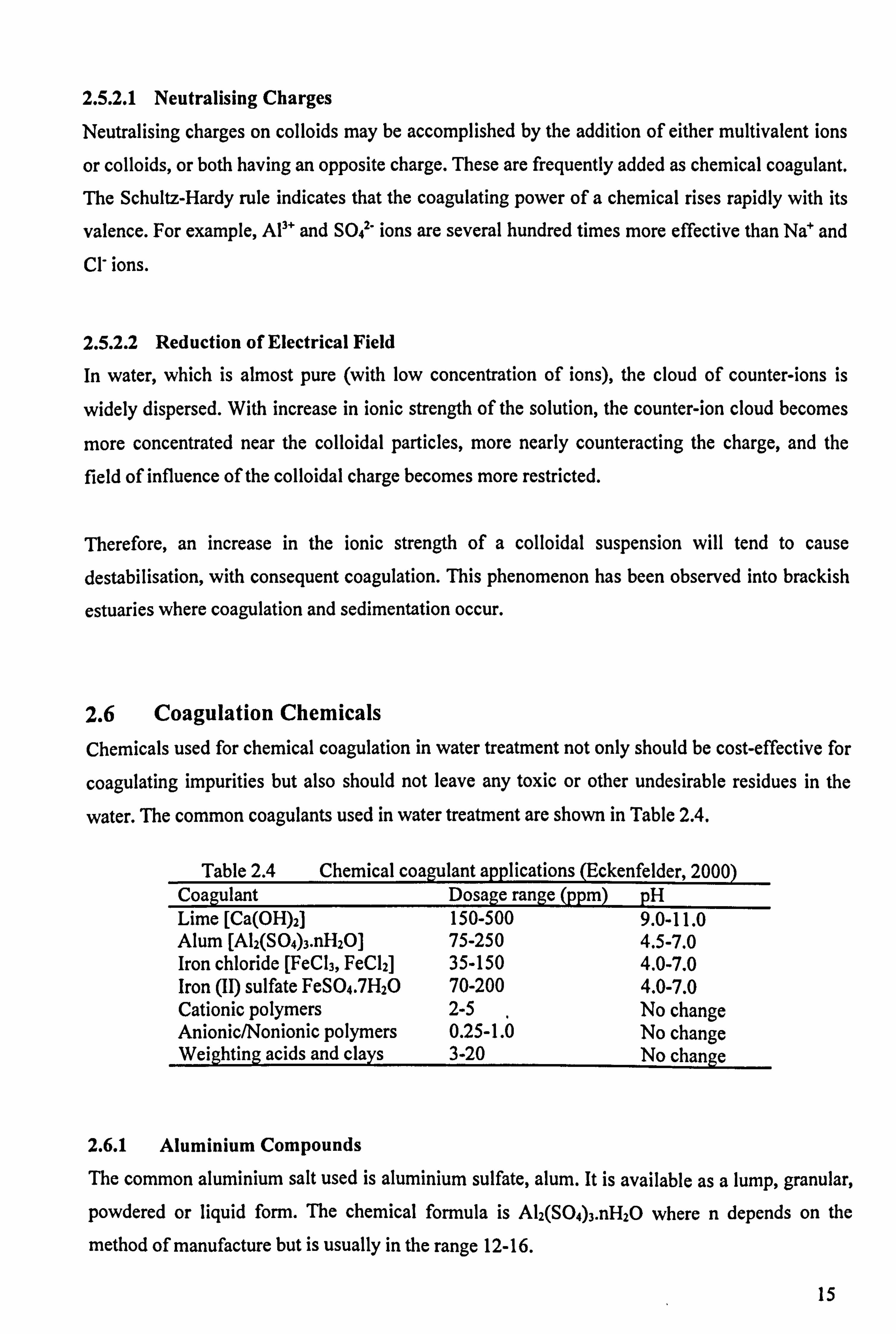
2.5.2.1 Neutralising Charges
Neutralising charges on colloids may be accomplished by the addition of either multivalent ions
or colloids, or both having an opposite charge. These are frequently added as chemical coagulant.
The Schultz-Hardy rule indicates that the coagulating power of a chemical rises rapidly with its
valence. For example, Al" and SOa2- ions are several hundred times more effective than Na+ and
Cl" ions.
2.5.2.2 Reduction of Electrical Field
In water, which is almost pure (with low concentration of ions), the cloud of counter-ions is
widely dispersed. With increase in ionic strength of the solution, the counter-ion cloud becomes
more concentrated near the colloidal particles, more nearly counteracting the charge, and the
field of influence of the colloidal charge becomes more restricted.
Therefore, an increase in the ionic strength of a colloidal suspension will tend to cause destabilisation, with consequent coagulation. This phenomenon has been observed into brackish
estuaries where coagulation and sedimentation occur.
2.6 Coagulation Chemicals
Chemicals used for chemical coagulation in water treatment not only should be cost-effective for
coagulating impurities but also should not leave any toxic or other undesirable residues in the
water. The common coagulants used in water treatment are shown in Table 2.4.
Table 2.4 Chemical coagulant applications (Eckenfelder, 2000 Coagulant Dosage range (ppm) pH Lime [Ca(OH)2] 150-500 9.0-11.0 Alum [A12(SO4)3. nH2O] 75-250 4.5-7.0 Iron chloride [FeC13, FeC12] 35-150 4.0-7.0 Iron (II) sulfate FeSO4.7H20 70-200 4.0-7.0 Cationic polymers 2-5 No change Anionic/Nonionic polymers 0.25-1.0 No change Weighting acids and clays 3-20 No change
2.6.1 Aluminium Compounds
The common aluminium salt used is aluminium sulfate, alum. It is available as a lump, granular,
powdered or liquid form. The chemical formula is A12(SO4)3. nH2O where n depends on the
method of manufacture but is usually in the range 12-16.
15

When hydrolysed, alum produces sulfuric acid (H2S04) as well as the hydroxide. It is therefore
regarded as an acid salt and the water must contain enough alkalinity (natural or added) to react
with the acid as it forms, to maintain the coagulation/flocculation pH within the desired range.
Figure 2.8 show the equilibrium compositions of solutions in contact with freshly precipitated Al
(OH)3 and Fe(OH)3. Calculated using representative values for the equilibrium constants for
solubility and hydrolysis equilibrium. Shaded areas are approximate operating regions in water
treatment practice; coagulation in these systems occurs under condition of over saturation with
respect to the metal hydroxide.
C
Y O
1 .6 s
o -: 0 s w_ M .1 0
-1.
-14L 0 2468 10 12 14
ý' Y O 8
T
rr+ C
d
M O
AI(O 11)ý ý ý1
-2
1(011);
-a
"6
I 1 I I I ;
Al (O H) 12
IA A17(O H)144 AI(OIp
oz46a 10 12 14
pH p'1
Figure 2.8 Equilibrium compositions of solutions in contact with Al and Fe hydroxides
(Stumm and O'Melia, 1968)
2.6.1.1 Sodium Aluminate
Sodium aluminate is an alkaline salt made by treating aluminium oxide with caustic soda. The
simple hydrolysis reaction is:
NaAIO2 + 2H20 -* AI(OH)3+ NaOH
It can be used either with conjunction with alum or on its own in waters which do not have
enough natural alkalinity. However, the resulting coagulation may not be as good as when alum is used with an alkali, because the divalent sulfate ions introduced with the alum have a favourable influence on coagulation.
Fe(O H)y (. ý
Fe" e(OH)i
e(OH)3*
H)7 (OH)2t -e\
ý Fe(O H)=` \
16

2.6.2 Iron Coagulants
Several different iron compounds are used for the treatment of potable water depending on
circumstances such as the raw water quality, availability and cost. Commercial data of the more
common and interesting of these reagents is given in Table 2.5.
Table 2.5 Data for commercial iron coagulants (Twort et al., 1994)
Ferric sulfate
Ferric Chloride
Ferrous sulfate
Chlorinated Copperas
Magnetite'
Chemical formula Fe2(S04)3 FeCI3 FeSO4 FeSO4 (+C12) Fe304 State of product Solution Solution Solid Solution & gas Solid Fe content (%) 12 14-14.5 18 18 72 pH of product <1.0 <1.0 1.7 (saturated) 1.7 (saturated) - Coagulation pH range 4.0-9.0 4.0-9.0 8.5-10.0 4.0-10.0 4.0-6.0 §: (Schwertmann and Cornell, 1991)
2.6.2.1 Ferric sulfate
Ferric sulfate [Fe2(SO4)3] is an readily available product, which is a good colour remover at low
pH and can be used at very low temperatures (Smethurst, 1988).
2.6.2.2 Ferric Chloride
Ferric chloride [FeC13] is extremely corrosive when it reacts with water to produce hydrochloric
acid, and so is unpopular and difficult to handle. Its use in high pH waters can be very useful as it
acts as a weak acid (Smethurst, 1988).
2.6.2.3 Ferrous sulfate
Ferrous sulfate [FeSO4] or often referred as "copperas" is used on alkaline waters in combination
with sufficient lime to raise the pH to 8.5-10. Under alkaline conditions, ferrous ions (Fe2+) are
oxidised to ferric ions (Fe"). It is not widely used in water treatment (Smethurst, 1988).
2.6.2.4 Chlorinated Copperas
Chlorinated copperas is formed in theory from one part of chlorine that oxidises eight parts of ferrous sulfate, producing a mixture of ferric chloride and ferric sulfate. It can be used over a
wide pH range and can be used effectively where there is need for pre-chlorination (Smethurst, 1988).
17
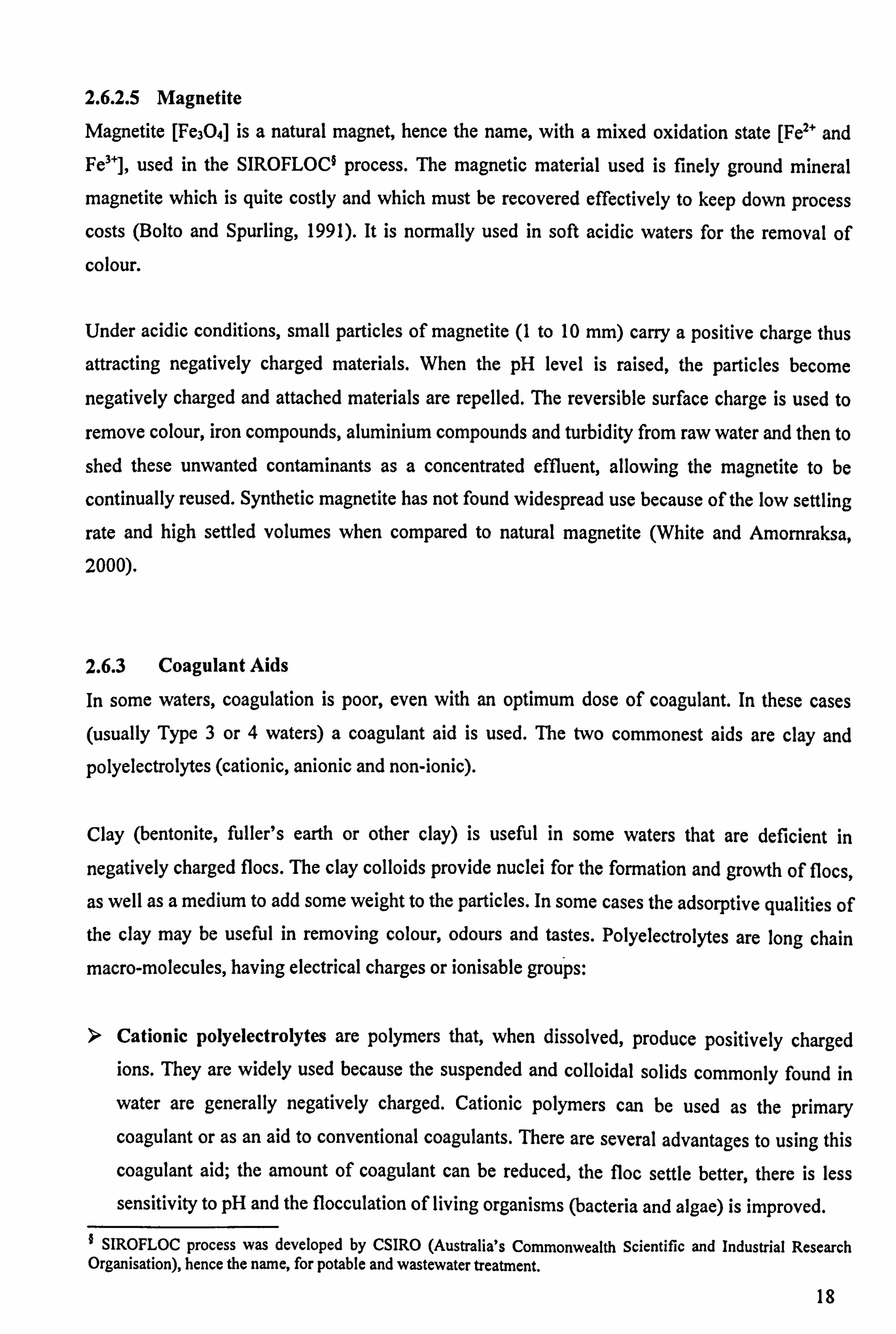
2.6.2.5 Magnetite
Magnetite [Fe304] is a natural magnet, hence the name, with a mixed oxidation state [Fe" and Fei+], used in the SIROFLOC§ process. The magnetic material used is finely ground mineral
magnetite which is quite costly and which must be recovered effectively to keep down process
costs (Bolto and Spurling, 1991). It is normally used in soft acidic waters for the removal of
colour.
Under acidic conditions, small particles of magnetite (1 to 10 mm) carry a positive charge thus
attracting negatively charged materials. When the pH level is raised, the particles become
negatively charged and attached materials are repelled. The reversible surface charge is used to
remove colour, iron compounds, aluminium compounds and turbidity from raw water and then to
shed these unwanted contaminants as a concentrated effluent, allowing the magnetite to be
continually reused. Synthetic magnetite has not found widespread use because of the low settling
rate and high settled volumes when compared to natural magnetite (White and Amornraksa,
2000).
2.6.3 Coagulant Aids
In some waters, coagulation is poor, even with an optimum dose of coagulant. In these cases (usually Type 3 or 4 waters) a coagulant aid is used. The two commonest aids are clay and
polyelectrolytes (cationic, anionic and non-ionic).
Clay (bentonite, fuller's earth or other clay) is useful in some waters that are deficient in
negatively charged flocs. The clay colloids provide nuclei for the formation and growth of flocs,
as well as a medium to add some weight to the particles. In some cases the adsorptive qualities of the clay may be useful in removing colour, odours and tastes. Polyelectrolytes are long chain macro-molecules, having electrical charges or ionisable groups:
> Cationic polyelectrolytes are polymers that, when dissolved, produce positively charged ions. They are widely used because the suspended and colloidal solids commonly found in
water are generally negatively charged. Cationic polymers can be used as the primary coagulant or as an aid to conventional coagulants. There are several advantages to using this
coagulant aid; the amount of coagulant can be reduced, the floc settle better, there is less
sensitivity to pH and the flocculation of living organisms (bacteria and algae) is improved.
SIROFLOC process was developed by CSIRO (Australia's Commonwealth Scientific and Industrial Research Organisation), hence the name, for potable and wastewater treatment.
18

> Anionic polyelectrolytes are polymers that dissolve to form negatively charged ions, and are
used to remove positively charged solids. Anionic polyelectrolytes are used primarily as
coagulant aids with aluminium or iron coagulants. The anionic polyelectrolytes increase floc
size, improve settling and generally produce a stronger floc. They are not materially affected by pH, alkalinity, hardness or turbidity.
> Non-ionic polyelectrolytes are polymers having a balance or neutral charge, but upon dissolving release both positively and negatively charged ions. Non-ionic polyelectrolytes
may be used as coagulants or as coagulant aids. Although they must be added in larger doses
than other types, they are less expensive.
Compared with other coagulant aids, the required dosages of polyelectrolytes are extremely
small. The normal dosage range of cationic and anionic polymers is 0.1 to 1 mg/L. For non-ionic
polymers the range is 1 to 10 mg/L. The mode of actions, which can occur with polymers and
colloidal material, is shown in Figure 2.9
Time
" Floc particle `'A Polyelectrolyte
Figure 2.9 The action of a polyelectrolyte coagulation/flocculation aid (Behl et al., 1993)
2.6.4 Chemical Precipitation
The advantages of the coagulation is that it reduces the time required to settle out suspended
solids and is very effective in removing fine particles, which are otherwise very difficult to
remove from water.
In addition, coagulation can also be effective in removing protozoa, bacteria and viruses, particularly when polyelectrolyte is used, as the highly charged coagulant attracts the charged microorganisms into the flocs. Coagulation can also be useful in removing by precipitation certain contaminants such as lead and barium.
19
The principal disadvantages of using coagulants are the volumes of sludge production and the
need for accurate dosing (jar testing and dose adjustment and frequent monitoring). Coagulants
can be expensive to buy (particularly polyelectrolytes) and need accurate dosing equipment to
function efficiently. Staff needs to be adequately trained to carry out jar tests to determine
coagulant dosage.
2.7 Disinfection
Disinfection is carried out to destroy the microbiological agents, which cause disease. It differs
from sterilisation, which implies the destruction of all micro-organisms. Water supplies are
usually disinfected.
The widespread adoption of disinfection was a major factor in reducing waterborne diseases, and
this has been interpreted as the major single factor in increasing average human life expectancy
globally.
2.7.1 Requirements of a Disinfectant
Chlorination usually performed, as the final treatment process is the most common means of
disinfecting drinking water. Other processes, natural and artificial, aid in the destruction or
removal of pathogens.
Most pathogens are accustomed to living in the temperatures and conditions in the bodies of humans and animals; they do not survive well outside such environments. Nonetheless,
significant numbers can survive in potable water.
Some pathogens, particularly certain viruses and those organisms that form cysts, can survive for
surprisingly long periods even under the most adverse conditions. Because such organisms also
tend to be resistant to chlorine doses normally used in water treatment, chlorination alone cannot
always ensure safe drinking water.
Storing water for extended periods in open tanks or reservoirs prior to treatment can accomplish
some destruction of pathogens through sedimentation and natural die-off of the organisms.
Significant pathogen removal occurs in the water treatment process.
20

A disinfectant must be able to destroy particular pathogens at the concentrations likely to occur,
and it should be effective in the normal range of environmental conditions. Disinfectants that
require extremes of temperature or pH, or which are effective only for low turbidity waters, are
unlikely to suitable for large-scale use.
While the disinfectant should destroy pathogens, it must not be toxic to man or other higher
animals, such as fish, in a receiving water. Ideally, some residual disinfecting capacity should be
provided for a water supply to provide protection against re-infection while the water is in the
distribution system. The residual that passes to the consumer should be neither unpalatable nor
obnoxious.
Nonetheless, a disinfectant should be safe and easy to handle, during both storage and addition. The other major consideration is that of cost, which is particularly important for municipal plants
where large volumes are commonly disinfected continuously.
2.7.2 Methods of Disinfection
Although chlorination is the most common technique for disinfection, other methods are
available and may be useful in some situations. Three general types of disinfection available are
as follows:
1. Heat treatment - boiling, pasteurisation (>60°C) and autoclaving (> 100°C);
2. Radiation treatment - ultraviolet, and; 3. Chemical treatment - bromine, iodine, ozone, chlorine dioxide and chlorine.
Chlorine is the most widely used chemical disinfectant. It has found widespread use not only for large and small water supply systems, but also for the treatment of swimming pool waters and
effluent disinfection.
2.7.2.1 Chlorine as a Disinfectant
Chlorine is available in gaseous and liquid forms. Under normal conditions, chlorine is a green- yellow, corrosive gas with a density 2.5 times that of air. It can be liquefied under a relatively small pressure (3.7 atmospheres). The gas is very soluble in water and is a potent disinfectant
even at low concentrations. When dissolved in water, chlorine forms two acids by reaction with
molecules of water as shown in Equation 2.2.
21

C12 +H20--* H+ + Cl' + HOC! Equation 2.2
Hypochlorous acid (HOCI) is a weak acid amd which is also a disinfecting agent and is referred
to as free available chlorine. Both the acids can dissociate to produce their respective anions and
protons.
For hypochlorous acid this dissociation is important, since the hypochlorite ion (CIO-) is not the
stronger disinfectant, Equation 2.2. The hypochlorous acid is 50% dissociated at pH 7.5 as shown
in Figure 2.10. To ensure effective disinfection, the pH must be acid so that at least 90% is in the
undissociated, active disinfectant form (at pH 5, it is undissociated).
0 Ü O
x
100
90
80
70
60
50
40
30
20
10
0
0
10
20
30
20°C 40
Nt 50
60 0
70
80
90
100
456789 10 11
pH
Figure 2.10 Variation of hypochlorous acid and hypochlorite ion system with pH (Sawyer and McCarty, 1994)
Chlorine is the most widely used chemical disinfectant. Chlorine rapidly penetrates microbial
cells and kills the micro-organism, through cell cysts. However, the effectiveness of chlorine is
influenced by the physical and chemical characteristics of the water.
The presence of suspended solids or the clustering of micro-organisms may protect pathogens
and so reduce the disinfecting ability. Chlorine is a strong oxidising agent and any reducing
agents, such as nitrates, ferrous ions and hydrogen sulfite, rapidly react with it, reducing the
concentration available to destroy pathogens.
22
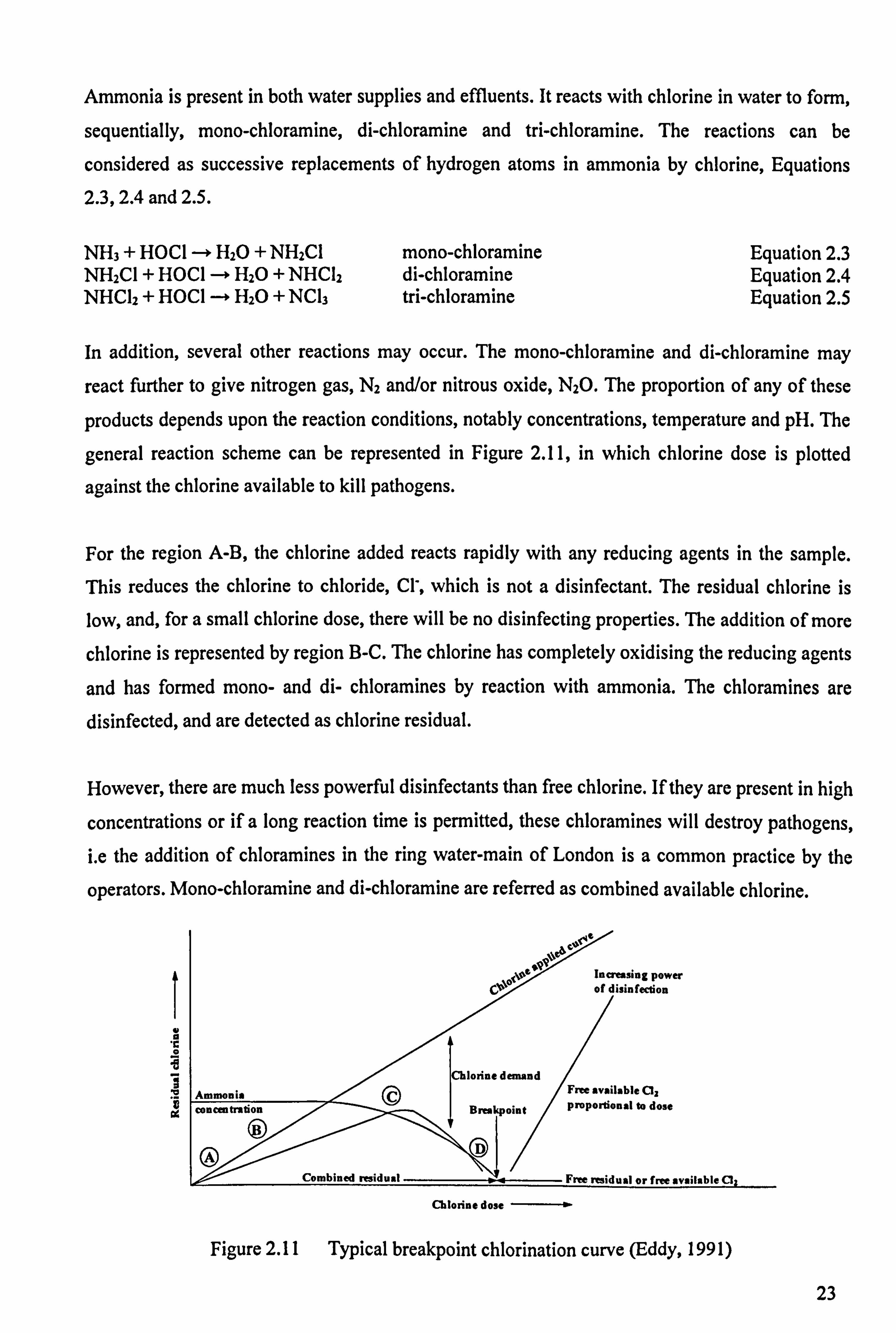
Ammonia is present in both water supplies and effluents. It reacts with chlorine in water to form,
sequentially, mono-chloramine, di-chloramine and tri-chloramine. The reactions can be
considered as successive replacements of hydrogen atoms in ammonia by chlorine, Equations
2.3,2.4 and 2.5.
NH3 + HOCI --º H20+ NH2C1 mono-chloramine Equation 2.3 NH2C1 + HOCI --º H20+ NHCl2 di-chloramine Equation 2.4 NHC12 + HOCI --º H20+ NC13 tri-chloramine Equation 2.5
In addition, several other reactions may occur. The mono-chloramine and di-chloramine may
react further to give nitrogen gas, N2 and/or nitrous oxide, N20. The proportion of any of these
products depends upon the reaction conditions, notably concentrations, temperature and pH. The
general reaction scheme can be represented in Figure 2.11, in which chlorine dose is plotted
against the chlorine available to kill pathogens.
For the region A-B, the chlorine added reacts rapidly with any reducing agents in the sample.
This reduces the chlorine to chloride, Cl', which is not a disinfectant. The residual chlorine is
low, and, for a small chlorine dose, there will be no disinfecting properties. The addition of more
chlorine is represented by region B-C. The chlorine has completely oxidising the reducing agents
and has formed mono- and di- chloramines by reaction with ammonia. The chloramines are
disinfected, and are detected as chlorine residual.
However, there are much less powerful disinfectants than free chlorine. If they are present in high
concentrations or if a long reaction time is permitted, these chloramines will destroy pathogens, i. e the addition of chloramines in the ring water-main of London is a common practice by the
operators. Mono-chloramine and di-chloramine are referred as combined available chlorine.
t `O
Increasing power
I ýjh of disinfection
V C O
Chlorine demand 2 Ammonia Free available C12
ä Concentration Breakpoint proportional to dose
Combined residual Free residual or free av
Chlorine dose --- º
Figure 2.11 Typical breakpoint chlorination curve (Eddy, 1991)
23

In the region B-C, the addition of chlorine produces an approximately proportional increase of
combined chlorine residual. Further addition of chlorine produces tri-chloramine, as per Equation
1.5, nitrogen, nitrous oxide and other products that are not disinfectants. Thus in the region C-D,
the addition of further chlorine reduces the available chlorine, and hence, the ability of the
solution to destroy pathogens.
On further chlorine addition, these reactions are complete, point D, and the ammonia is
completely oxidised. Any subsequent addition of chlorine will remain as free available chlorine
(HOCI) if the pH is correct and will act as a strong chlorine residual. Point D is referred to as the
breakpoint.
Appreciable amounts of combined residuals still exists beyond the breakpoint. However, these
combined residuals mainly consist of combined chloro-organics and combined organic
chloramines, which have little or no disinfecting properties.
The practice of chlorinating up to and beyond the breakpoint is called superchlorination.
Superchlorination ensures complete disinfection. However, it will leave free chlorine residuals in
the distribution system, which can simply disappear very quickly.
If superchlorination is to be practiced to ensure complete disinfection and it is also desired to
have long-lasting chlorine residuals, then ammonia should be added after superchlorination to
bring back the chlorine dosage to the point of maximum monochloramone formation.
The chlorine-ammonia reaction as set out in Figure 2.11 should be regarded as a simplified
representation. The free and combined residual concentrations depend upon the reaction
conditions for any particular sample.
2.7.2.2 The Kinetics of Chlorination
The ability of a reagent to destroy pathogens is related to the concentration of the disinfectant and the contact time between the pathogens and disinfectant. One general relationship known as Chick's Law (Equation 2.6), which assumes that the distribution of micro-organisms is
controlled by processes of diffusion:
dN =_klV dt
Equation 2.6
24
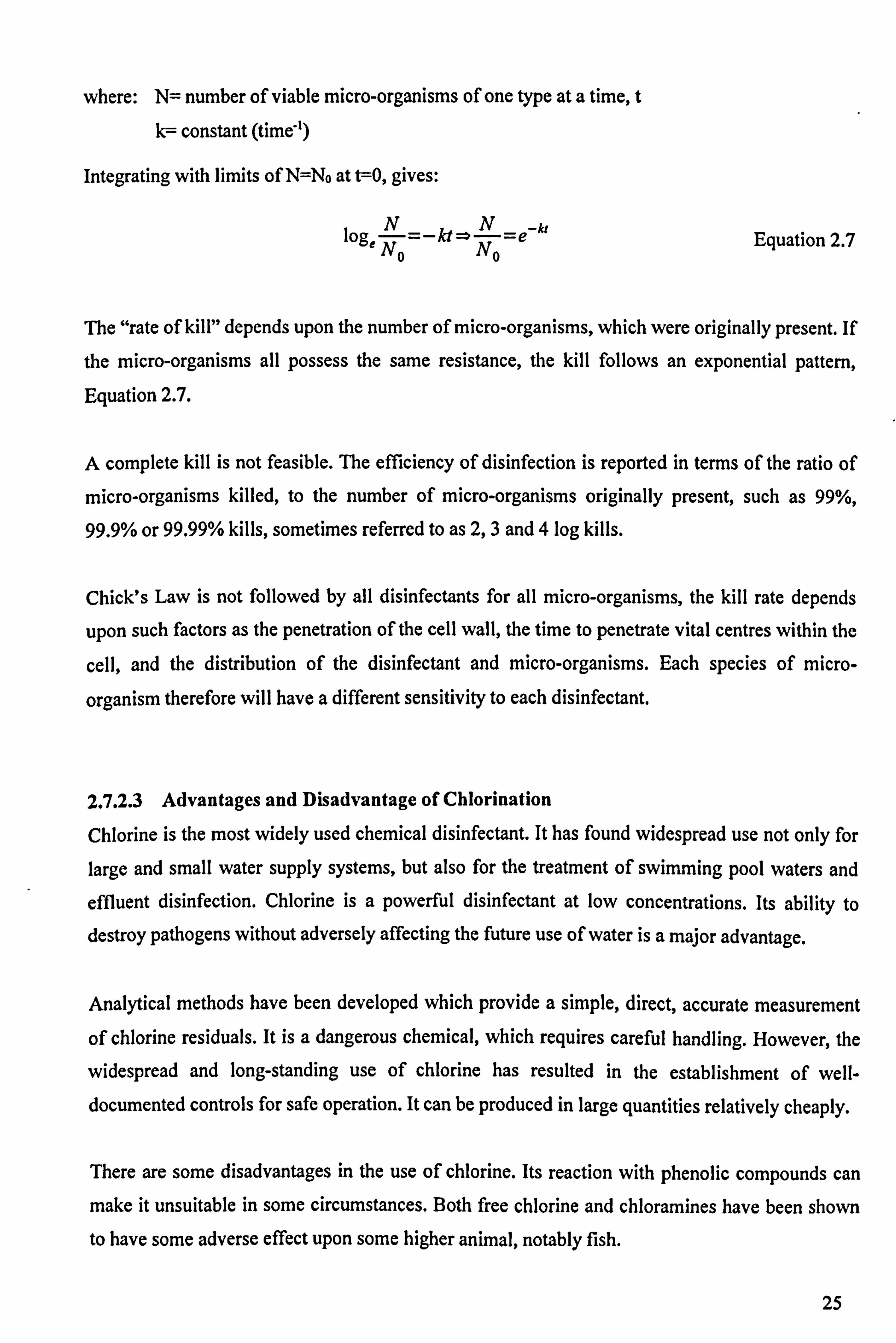
where: N= number of viable micro-organisms of one type at a time, t
k= constant (time')
Integrating with limits of N=No at t=0, gives:
loge N __k
N =e-k' Equation 2.7 No No
The "rate of kill" depends upon the number of micro-organisms, which were originally present. If
the micro-organisms all possess the same resistance, the kill follows an exponential pattern, Equation 2.7.
A complete kill is not feasible. The efficiency of disinfection is reported in terms of the ratio of
micro-organisms killed, to the number of micro-organisms originally present, such as 99%,
99.9% or 99.99% kills, sometimes referred to as 2,3 and 4 log kills.
Chick's Law is not followed by all disinfectants for all micro-organisms, the kill rate depends
upon such factors as the penetration of the cell wall, the time to penetrate vital centres within the
cell, and the distribution of the disinfectant and micro-organisms. Each species of micro-
organism therefore will have a different sensitivity to each disinfectant.
2.7.2.3 Advantages and Disadvantage of Chlorination
Chlorine is the most widely used chemical disinfectant. It has found widespread use not only for
large and small water supply systems, but also for the treatment of swimming pool waters and
effluent disinfection. Chlorine is a powerful disinfectant at low concentrations. Its ability to
destroy pathogens without adversely affecting the future use of water is a major advantage.
Analytical methods have been developed which provide a simple, direct, accurate measurement
of chlorine residuals. It is a dangerous chemical, which requires careful handling. However, the
widespread and long-standing use of chlorine has resulted in the establishment of well- documented controls for safe operation. It can be produced in large quantities relatively cheaply.
There are some disadvantages in the use of chlorine. Its reaction with phenolic compounds can
make it unsuitable in some circumstances. Both free chlorine and chloramines have been shown to have some adverse effect upon some higher animal, notably fish.
25

In addition, chlorination has been shown to produce trihalomethanes (THMs) compounds such as
chloroform, CH3C1, by reaction with organic matter in the water. These compounds are known
carcinogens. Moreover, chlorine is not notably effective in removing certain tastes, odours and
colour from water, neither will chlorine in normal use kill Cryptosporidium. Chlorine will
continue to be a popular and wide-spread disinfectant, however, other disinfectants and oxidants
should also be considered and their performance and cost compared to chlorine.
2.7.2.4 Disinfection Using Ozone
Ozone is a very strong oxidizer and has been found to be superior to chlorine in inactivating
resistant strains of bacteria and viruses. It is very unstable, however having a half-life of only 20-
30 minutes in distilled water. It is therefore generated on site before use. Ozone treatment has the
ability to achieve higher levels of disinfection than either chlorine or ultraviolet, however, the
capital costs as well as maintenance expenditures are not competitive with available alternatives.
2.7.2.5 Disinfection Using Ultraviolet Light
Water, air, and foodstuff can be disinfected using ultraviolet light, UV. This radiation destrroys
bacteria, bacterial spores, molds, mold spores, viruses, and other microorganisms. The unit
operations in UV disinfection involve the generation of the UV radiation and its insertion into or
above the flowing water stream to be disinfected. The contact time is very short, being in the
range of seconds to a few minutes. To be effective, the sheet of flowing water should be thin, so
that radiation can penetrate.
2.8 Water Supply
Once water has been abstracted, treated and disinfected, it is ready to be distributed to the
customers. A water supply system must deliver enough water of high quality at sufficient
pressure for domestic, commercial, industrial, and municipal uses.
Needs must be met during peak demand periods and during drought, as well as during periods of
average supply and demand. In addition, standby water for fire fighting is essential. A percentage
of the water is normally unaccounted for through leakage and other losses (Mays, 2000).
26

A water supply distribution network is made up of pumps, piping, water tanks, and supply
networks whose individual efficiency must be attuned to each other. Several types of pipe
materials are used in transmission and distribution systems.
Design criteria include strength, durability, corrosion resistance, flow capacity, cost,
maintainability, and effect on water quality. Common materials and some of their characteristics
are given in Table 2.6.
Table 2.6 Pipe materials used in transmission and distribution systems (AWWA, 1996 Pipe Material Uses and Characteristics Asbestos cement Used in smaller sizes, easy to handle, might damage easily or
deteriorate under aggressive soils Cast iron (lined/unlined) They are used in smaller sizes and are strong, easily tapped,
and subject to corrosion Concrete (prestressed) Used up to very large sizes, durable, may deteriorate in some
soils Concrete (reinforced) Used more for transmission lines than distribution lines. Used
up to very large sizes, durable, may deteriorate in some soils Polyvinyl chloride (PVC) Used in distribution systems. Lightweight. Easy to install and
resists corrosion. Care require when handling Steel Used more for transmission lines than distribution lines. Found
in wide range of sizes, up to very large. Adaptable to many conditions, subject to corrosion
The pipes must be capable of transferring the required flow, be capable of withstanding internal
pressure created by pumping without bursting and when laid under roads be capable of
withstanding the crushing loadings imparted by vehicle traffic.
Pipes must also be suitable to withstand accidental damage caused by mechanical and manual
digging, a common problem in urban areas. Metal pipes, on the other hand, must be protected
against corrosive action by groundwater and soils.
Potable water deterioration and/or contamination may also occur form the piping material used
inside a building when water remains stationary too long. Thus, it is extremely important to
choose the correct piping material that is appropriate for the expected quality the water source.
Most often pipes made of galvanised steel or copper are used.
Lead pipes are commonly found in old houses. Lead piping was used for the service connections
used to join residences to public water supplies. Lead piping is more likely to be found in homes
built before 1930. Copper piping replaced lead piping, but lead based solder was used to join
copper piping (Sawyer and McCarty, 1994).
27

Today, brass materials are used in all residential, commercial and municipal water distribution
systems. Many household taps, plumbing fittings, check valves and well pumps are manufactured
with brass parts.
2.9 Summary
This Chapter begins by defining sources of raw water, and the physico-chemical treatment of
water. In addition, it examines the requirements of the levels of performance of the water treatment plants, which are mostly driven by government laws and regulations.
This Chapter applies the techniques of the unit process of coagulation to the treatment of water
for the removal of colloids. It also discusses prerequisite topics necessary for the understanding
of coagulation such as the behaviour of colloids, and colloidal stability. The colloid particles are
the cause of the turbidity and colour that make waters objectionable, thus, should at least be
partially removed.
Following coagulation, disinfection is the unit process involving reactions that render pathogenic
organisms harmless. Because chlorine is the most widely disinfectant, its chemistry is discussed
at length.
28

lý'J (W
J, cceeeee
Potassium ferrate has been evaluated as a multi-functional wastewater treatment chemical for
disinfection, oxidation, and coagulation (DeLuca et al., 1983); Waite, 1981; Murmann and
Robinson, 1974). Research studies have indicated that potassium ferrate is also a more effective
coagulant than other inorganic coagulants such as aluminium, ferric or ferrous salts (DeLuca et
al., 1992; Waite, 1981; Waite and Gray, 1984).
3.1 Ferrate (VI)
The best-known member among the family of iron (VI) derivatives is potassium ferrate
(K2FeO4). The properties of high stability and low solubility of K2FeO4 in a saturated solution of
potassium hydroxide (KOH) helps its preparation (Moeser, 1897). Because of its relatively high
stability, K2FeO4 is used to prepare other ferrates such as SrFeO4 (Scholder, 1962), BaFeO4
(Gump et al., 1954) and Ag2, FeO4 (Firouzabadi et al., 1986).
On the other hand, sodium ferrate (Na2FeO4) has a behaviour different from those of other
ferrates and remains soluble in an aqueous solution saturated in sodium hydroxide (Delaude and
Laszlo, 1996).
Thus, the preparation of Na2FeO4 from an aqueous medium is made difficult and leads to rather impure samples. Rigorous control of the experimental conditions is required in order to minimise
the amount of iron (III) and iron (IV) derivatives formed as by-products contaminating the
desired iron (VI) salt (Kiselev et al., 1989).
Potassium ferrate provides a better entry into the group of iron (VI) derivatives. The salt
preparation in aqueous solution takes advantage of both the stability of the ferrate dianion in
alkali medium and the insolubility of potassium ferrate in a saturated solution of potassium hydroxide. This ensures both formation and isolation through precipitation of potassium ferrate.
29

3.2 Iron Oxidation States
Iron is the only compound that has an oxidation state equal to the total number of valence shell
electrons, which in this case are eight. The eight possible oxidation states of iron include (-11),
(0), (I), (II), (III), (IV), (V) and (VI).
All these oxidation states have different electronic configurations, co-ordination numbers and
geometries (Cotton and Wilkinson, 1999). However, apart from metallic iron, only two iron ions
have stable aqueous chemistry, the iron (II) and the iron (III) ion. Ferrate (VI) is stable for E
values from 0 to 1V and for pH values larger than 5.5, as shown in the Pourbaix diagram for
iron shown in Figure 3.1.
2.0
1.50H
A
Fei` 1.0
0.50- FeOHz'
B 0.0 V- I Fe(Ofih'
FeO4'
Fez+ H Fe02'
-0.50-1
-1.0 If
7i 0123456789 10 11 12 13 14
pH
. A-A' and B-B' represent the top and bottom respectively of the stable water region
Figure 3.1 Pourbaix diagram for iron in aqueous solution (Pourbaix, 1966)
Such E-pH stability field diagrams show in a comprehensive way how protons and electrons
simultaneously shift the equilibria under various conditions and can indicate which species
predominate under any given condition of E and pH.
Of course, such a diagram, like all other equilibrium diagrams, represents only the information
used in its construction. Nonetheless, equilibrium diagrams can greatly aid attempts to
understand the possible redox patterns in natural waters and in water treatment systems.
30

3.2.1 Iron (II)
The old name for iron (II) ion is ferrous. Iron (II) forms salts with most anions. Generally, the
salts are white or green crystalline solids. Frequently, salts will turn dark green, then brown over
time as Fe2+ ion is oxidised to Fe3+ by oxygen, as shown in Equation 3.1, or by loss of the
hydration water. Iron (II) can be also oxidised to iron (III) by other common oxidants, in both
acidic and basic conditions (Cotton and Wilkinson, 1999).
2Fe2+ +V2 OI + 2H+ --º 2Fe3+ +H20
3.2.2 Iron (III)
Equation 3.1
The old name for iron (III) ion is ferric. Iron (III) forms salts with most anions, except those with
strong reducing capacity. Generally, the salts are pale pink to nearly white crystalline solids. Iron
(III) in aqueous solutions has a distinctive tendency to hydrolyse and/or to form complexes.
At a pH close to 0 (pH<1), no hydrolysis takes place and there is only species is the pale purple
free ion. At a pH>2, hydrolysis starts to occur leading to precipitation of red brown hydrous
oxide, Fe203, while at a pH>3, yellow hydroxo species are formed (Housecroft and Sharpe,
2001).
3.2.3 Iron (VI)
Iron (VI) or ferrate salts has been known for over a century, but its chemistry is relatively
unexplored considering its tetrahedral ion Fe042" is isostructural with chromate and
permanganate (Hoppe et al., 1982). Ferrate is a powerful oxidising agent and the oxidising power increases from Cr to Mn, as shown in Table 3.1.
Table 3.1 Redox potentials of ferrate
Oxidants pH<2 pH= 7 pH>8 Reference Fe (VI) / Fe (III) couple 2.20 0.72 (Wood, 1958) Fe (VI) / Fe (III) couple 1.90 0.90 (Johnson and Read, 1996) Fe (VI) / Fe (III) couple 1.40 (Stupin and Ozernoi, 1995) Cr (VI) / Cr (III) couple 1.33 -0.12 (Delaude and Laszlo, 1996)
Mn (VII) / Mn (IV) couple 1.679 0.588 (Delaude and Laszlo, 1996)
31

Although from its redox potentials and structure one might anticipate its chemistry to be
essentially identical with that of permanganate or chromate, there are significant differences in its
reactivity.
Because of these high potentials, ferrate rapidly oxidises a variety of inorganic and organic
contaminants. In the absence of a suitable reductant, ferrate will react with water to form Fe (III)
and molecular oxygen, as shown in Equation 3.2 (Williams and Riley, 1974).
4FeO4Z" +1 OH20 -> 4Fe(OH)3 + 80H- + 302 Equation 3.2
3.2.4 Iron Oxides and Hydroxides
Iron is one of the few elements that can form a number of oxides, hydroxides and oxyhydroxides.
There are eight major naturally occurring iron oxides, each of them having different
characteristics due to different iron oxidations states and crystal structures, as shown in Table
3.2. Density in particular can affect settling rate and sludge formation.
Table 3.2 Characteristics of iron oxides (Housecroft and Sharpe, 2001) Mineral Empirical Formula Density (g/cm3) Akaganeite Fee+Oo. s(OH)1.2Clo. 2 3 Feroxyhyte Fe 3+0(OH) 4.2 Ferrihydrite Fei+203.0.5 (HBO) 3.8 Goethite Fe 3+0(01-1) 3.3-4.3 Hematite Fei+2O3 5.3 Lepidocrocite Fe 3+0(OH) 4 Maghemite Fei+2O3 4.9 Magnetite Fei+2Fe2+O4 5.15
3.3 Ferrate Structure
In aqueous solutions, the infrared spectrum of ferrate is consistent with a tetrahedral geometry (Griffith, 1966) and isotopic oxygen exchange studies have indicated that all oxygens are kinetically equivalent (Goff and Murmann, 1971).
From the knowledge that metal-oxygen bonds are strongly polarised LM =OH L�M+ - 0-
(Howard and Parkin, 1994), it can be concluded that the ferrate ion is best visualised as a
positively charged iron cation surrounded by four equivalent oxygens, each bearing a partial
negative charge; i. e. a resonance hybrid of three canonical structures, a-c, as shown in Figure 3.2.
32

o_+ 0- 0
Fe V0J eÖ
O" Ö
Figure 3.2 Ferrate structure (Norcross et al., 1997)
An independent study using symmetry adapted cluster predicted that the charge on the central
metal of comparable compounds ranges from 1.04 to 1.44, suggesting that both 2 and 3 strongly
contribute to the structure of ferrate (Jitsuhiro et al., 1994).
3.4 Ferrate Properties
Pure potassium ferrate (VI) is a dark, reddish-black powder exhibiting numerous silvery
iridescent flashes due to the reflection of light by the small crystals. Dry potassium ferrate (VI) is
stable at temperatures below 198°C (Haire, 1965). Potassium ferrate (VI) is very soluble in water,
giving a blood-red solution with a colour intensity comparable to that of potassium permanganate
solutions (Caddick et al., 2000).
In aqueous solution, the ion remains monomeric, and its four oxygen atoms become equivalent
and exchange slowly with the solvent (Goff and Murmann, 1971). In acidic or neutral solution
the ferrate ions are quickly reduced by water. Oxygen is evolved, and ferric complexes and
precipitating hydrous iron (III) oxide, are formed, as summarised in Equation 3.3. The alkalinity
of the solutions increases as decomposition proceeds.
4K2FeO4 + 10H20 -). 4Fe(OH)3 + 302T + 8KOH Equation 3.3
In basic solution, the rate of decomposition of ferrate is highly variable; temperature and pH are key factors. Light does not affect the stability of ferrate solutions (Wagner et al., 1952; Schreyer
and Ockerman, 1951). In 1993, Lee and Gai carried out precise kinetic measurements and found
that, in dilute solution, the lowest rate of ferrate reduction by water occurs between pH 9.4 and 9.7.
33

Potassium ferrate is insoluble in common organic solvents. It can be suspended in ether,
chloroform, benzene, and other solvents without rapid decomposition. Alcohols may also be
used, provided that they do not contain more than 20% water. Above this limit, fast
decomposition ensues, and aldehydes or ketones are formed (Lee and Gai, 1993).
3.5 Synthesis of Ferrate
As early as 1702, it was mentioned by the German chemist and physician Stahl the appearance of
an unstable purplish red colour when the molten mass (mixture of saltpetre and iron) was dissolved in water.
In 1834, Eckeberg and Becquerel both found that a solid resulting from the fusion of iron oxide
with potassium hydroxide when dissolved in water, formed a purplish red colour solution, which decomposed with the evolution of oxygen.
It was not until 1844 though, when Fremy suggested a formula of the Fe03 to the unknown
purplish-red compounds described above. Fremy was the first to form ferrate in solution by
passing chlorine gas through a concentrated solution of potassium hydroxide containing ferric
oxide. He proposed the reaction as shown in Equation 3.4. The systematic study of the synthesis
of ferrate (VI), however, started about 100 years ago (Moeser, 1897).
Fe203.3H2O + 10 KOH +3 C12 --> 2 K2FeO4 +6 KC1 +8 H2O Equation 3.4
In 1897, Moeser was the first to write a detailed review of ferrates and their chemistry describing
three methods of preparation of potassium ferrate, namely:
> Dry method - heating to red various potassium- and iron-containing minerals. Dry
reactions imply detonation and elevated temperatures, which are considered dangerous
and too difficult to implement;
> Electrochemical method - electrolysing a potash solution with an iron anode. This
method remains another access to ferrates that has retained only marginal interest.
Ferrate (VI) was prepared in an electrochemical way for the first time as early as 1841 by
Poggendorf. Since then, it has benefited from recent improvements though, such as
superposition of an alternative current to the direct current for electrolysis (Bouzek et al., 1998) and;
34

> Wet method - oxidising a basic solution of a Fe (III) salt by a hypochlorite or hypobromite.
Among the above three approaches, the wet method was the primary one in the 20' century. In
1948, Schreyer prepared potassium ferrate by bubbling chlorine through a potassium hydroxide
solution containing a suspension of hydrous ferric oxide.
In 1950, Hrostowski and Scott prepared potassium ferrate from solutions of ferric chloride and
sodium hypochlorite in the presence of sodium hydroxide. Addition of potassium hydroxide then
served to precipitate potassium ferrate from the sodium solution. The basic chemical reactions
are shown as follows in Equations 3.5,3.6, and 3.7:
Fei++ 3 OH- -º Fe(OH)3 Equation 3.5
2 Fe(OH)3 +3 NaC1O +4 NaOH -+ 2 Na2FeO4 +3 NaCl +5 H2O Equation 3.6
Na2FeO4 +2 KOH --* K2FeO4 +2 NaOH Equation 3.7
Although the ferrate purity was very high (96.9%), the ferrate yield remained very low (10-15%).
In 1951, Thompson et al. improved yields (45-75%) with no drop in purity, by simply modifying
the experimental procedure - chlorination of the potassium hydroxide solution prior to the
addition of ferric oxide.
The preparation protocol of Thompson et al. (1951) together with the analysis procedure (by a
redox titration) remain today the standard methodology for preparing and evaluating the purity of
potassium ferrate.
Further improvements of ferrate yield were studied by other researchers with many modifications
to the original method were made to combine high yields and purities while holding to a simple,
straightforward experimental procedure.
However, the most significant improvement did not come until 1974, when Williams and Riley
proposed bypassing the intermediate formation of sodium ferrate through use of potassium hydroxide and hypochlorite. The end product takes less time, and the yields are better (75%) but
at the cost of some loss in purity (80-90%). The purity and yield of the modified wet methods are
summarised in Table 3.3.
35

Table 3.3 Ferrate purities and yields from alternative wet methods Purity Yield Method Characteristics Reference
(%) (%)
96.9 10-15 Use of sodium ferrate (Hrostowski and Scott, 1950) 92-96 44-76 Potassium hydroxide chlorination (Thompson et al., 1951)
before the addition of ferric oxide 75+ 80-90 Use of potassium hydroxide (Williams and Riley, 1974)
It is also possible to produce ferric-iron salts from galvanising waste (Cici and Cuci, 1997).
These processes do not require complex systems due to their simple and economical
applicability.
International Reclamation Co. (INMETCO) has developed a process for reclaiming nickel,
chromium and iron from stainless steel wastes (Hanewald, 1985). In 1994, Arslan et al. studied
the production conditions of Fe203 from FeSO4. xH20 formed in galvanising works.
The ability to produce chemicals from galvanising waste offers the possibility of great savings in
raw materials and energy costs. On the other hand, pollution potential of metal finishing industry
would be minimised by eliminating the disposal problem at the source.
An alternative preparation of potassium ferrate using bleach would be highly desirable, as it
would avoid the requirement of chlorine gas. By using relatively strong bleach (12% available
chlorine), it has proved possible to prepare potassium ferrate in reasonable yield (20-30%) and
purity of >94% (Caddick et al., 2000).
3.6 Ferrate Characterisation
There are two major methods to characterise ferrate (VI) salts:
1. Volumetric titration method, and; 2. Spectroscopy method.
3.6.1 Volumetric Titration Method
Ferrate (VI)'s strong oxidising properties are used to determine the ferrate concentrations by
volumetric titration analysis. Ferrate salts can be reduced, either to the ferrous (Fe") ions or to
the ferric (Fe3+) ions by suitable ions, such as iodide, arsenite, and chromium.
36

3.6.1.1 Iodide Test
Iodide ion can reduce either or both of ferrate (VI) and ferric (Fe3+) ions to the ferrous ions (Fe2+),
and therefore, it is possible to measure the ferrate concentration. The drawback of this method is
coexisting ferric ions in ferrate salt will affect analytical results (Jiang and Lloyd, 2002).
3.6.1.2 Arsenite Test
In this method, the ferrate salt is reduced to ferric ion in an alkaline arsenite solution (excess of
arsenate to arsenite). The excess arsenite is then back titrated with standard bromate or cerate
solution, and therefore, it is possible to measure the ferrate concentration from the equivalent of
consumed bromate or cerate (Schreyer et al., 1950b).
3.6.1.3 Chromium Test
In this method, ferrate is used to oxidise excess of chromium (III) to chromium (IV) under
alkaline conditions. The solution is then acidified and titrated to find the amount of chromium
(VI) formed, and therefore, it is possible to measure the ferrate concentration from the equivalent
of formed chromium (VI) (Schreyer et al., 1950a).
3.6.2 Spectroscopy Method
Ferrate ions can easily be detected by their dark purple colour, which corresponds to the visible
and near infrared absorption spectrum at about 500 and 800 nm, Figure 3.3. The absorption
spectrum of potassium ferrate at 505 nm was confirmed by other investigators in their studies
(Carrington et al., 1957; Jia et al., 1999).
1 200
800
w 400
o+ 300
2-
\O
400 500 600 700 800 900 1000 Wavelength (nm)
Figure 3.3 Electronic spectrum of potassium ferrate (Carrington et al., 1957)
37
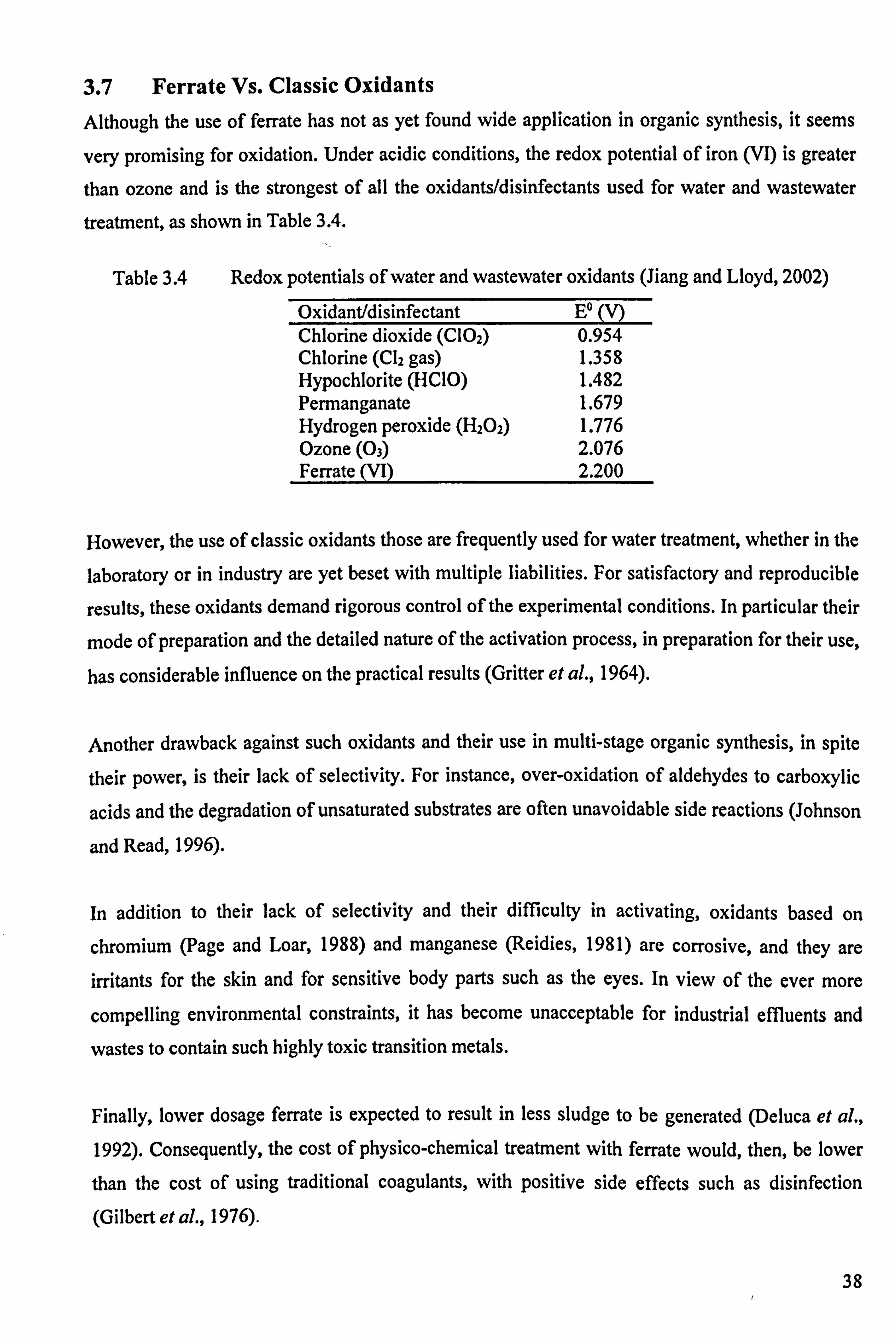
3.7 Ferrate Vs. Classic Oxidants
Although the use of ferrate has not as yet found wide application in organic synthesis, it seems
very promising for oxidation. Under acidic conditions, the redox potential of iron (VI) is greater
than ozone and is the strongest of all the oxidants/disinfectants used for water and wastewater
treatment, as shown in Table 3.4.
Table 3.4 Redox potentials of water and wastewater oxidants (Jiang and Lloyd, 2002)
Oxidant/disinfectant E° (V) Chlorine dioxide (CIO2) 0.954 Chlorine (Cl2 gas) 1.358 Hypochlorite (HC1O) 1.482 Permanganate 1.679 Hydrogen peroxide (H202) 1.776 Ozone (03) 2.076 Ferrate (VI) 2.200
However, the use of classic oxidants those are frequently used for water treatment, whether in the
laboratory or in industry are yet beset with multiple liabilities. For satisfactory and reproducible
results, these oxidants demand rigorous control of the experimental conditions. In particular their
mode of preparation and the detailed nature of the activation process, in preparation for their use,
has considerable influence on the practical results (Gritter et al., 1964).
Another drawback against such oxidants and their use in multi-stage organic synthesis, in spite
their power, is their lack of selectivity. For instance, over-oxidation of aldehydes to carboxylic
acids and the degradation of unsaturated substrates are often unavoidable side reactions (Johnson
and Read, 1996).
In addition to their lack of selectivity and their difficulty in activating, oxidants based on
chromium (Page and Loar, 1988) and manganese (Reidies, 1981) are corrosive, and they are irritants for the skin and for sensitive body parts such as the eyes. In view of the ever more
compelling environmental constraints, it has become unacceptable for industrial effluents and
wastes to contain such highly toxic transition metals.
Finally, lower dosage ferrate is expected to result in less sludge to be generated (Deluca et al., 1992). Consequently, the cost of physico-chemical treatment with ferrate would, then, be lower
than the cost of using traditional coagulants, with positive side effects such as disinfection
(Gilbert et al., 1976).
38
3.8 Ferrate in Water and Wastewater Treatment
Nowadays, there is a considerable interest in the development of new technology, for the
disinfection and removal of trace organic materials from potable water supplies and also the
removal of organics from aqueous process streams prior to recycle or discharge into natural
waters. Much of the driving force results from the perceived need to discontinue the use of
chlorine and chlorine derivatives for such purposes.
Fe (VI) has shown great promise as a multi-functional wastewater treatment chemical for
disinfection, oxidation and coagulation (Waite and Gray, 1984). It has been shown that ferrate
can remove toxic organic molecules such as nitrosamines (Bartzatt and Nagel, 1991), organic
sulphur compounds (Read et al., 2000) and phenol (Waite and Gilbert, 1978), as well as
inorganic ions such as cyanide (Sharma et al., 1998), destroy viruses (Schink and Waite, 1980)
and bacteria (Murmann and Robinson, 1974).
It is probably in this venue that ferrate holds its greatest promise for industrial application.
Investigation of removal of metals, non-metals, and radionuclides by iron (VI) has also been
conducted (Bartzatt et al., 1992; Potts and Churchwell, 1994).
3.8.1 Algae Reduction
Laboratory studies conducted by Ma and Liu (2002) demonstrated that pre-treatment of lake
water with potassium ferrate enhanced the algae removal by coagulation with alum. Algae
reduction efficiency increased remarkably, when the water was pre-treated with ferrate.
A very short time (1 minute) of pre-oxidation was enough to achieve substantial algae reduction
efficiency of 65 per cent, and the effectiveness was further increased up to 80 per cent at a
prolonged pretreatment time (20 minutes).
The coagulation was also improved by increasing particle concentration in water, because of the formation of the intermediate forms of precipitant iron species during pre-oxidation. In addition, it was also observed that ferrate pre-oxidation caused algae agglomerate formation before the
addition of coagulant, the subsequent application of alum resulted in further coagulation (Ma and Liu, 2002).
39

3.8.2 Fulvic Acid Reduction
Jar tests and pilot tests conducted by Qu et al. (2003) demonstrated that ferrate has a good
oxidation capacity for fulvic acids (FA) present in drinking water. The ultraviolet absorption (UVA) of 2 mg/L FA in water was found to be reduced by about 90% at a weight ratio of ferrate
to FA of 12: 1.
Adsorption to and coprecipitation with ferric hydroxide precipitate produced by ferrate
decomposition can also result in additional FA reduction. In the presence of turbidity, ferrate can
oxidize and adsorb simultaneously and over 95% of UVA was reduced with the same weight
ratio of 12: 1. Combining the application of ferrate and polyaluminum chloride (PAC) or iron
chloride (FeC13) was more effective for FA reduction and complete FA removal was achieved
(Qu et al., 2003).
3.8.3 E. coli.
The use of ferrate to disinfect water is entirely feasible in terms of germicidal efficiency,
particularly in waters with a pH below 8, although ferrate maintained adequate disinfecting
potential above pH 8.
E. coli was selected as most suitable for study by Gilbert et al. (1976) mainly because it is a
reference organism for most disinfection studies, even though E. coli may be less resistant to
chemical disinfectants than are Salmonella, Shigella and some enteroviruses. Figure 3.4 shows a Watson time concentration relationship for several organisms, including E. coli at pH 7.
a e
'C 0
0 V V e e V
Q F- a2
Figure 3.4
oureus
S. bovis B, caar
S.
-200
20 e w
e feawlis -2.0
e7%
E. cou fyphimuº! um
0.2
Time for 99% Inactivation (min)
Watson time-concentration relationship vs. K2FeO4 at pH=7 (Waite, 1978)
40

The Watson time-concentration relationship is an empirical relationship developed by Watson
and has been used to compare disinfectants as well as the relative resistances of organisms to
each other or to varied disinfecting conditions. This relationship is:
Cnt99- K
where C is the concentration of the disinfectant (mg/1), n is a constant known as the coefficient of dilution, t99 is the constant time required for 99% inactivation of the organism, and K is a
constant indicating the time required for 99% inactivation with 1mg/l disinfectant.
If n values are greater than unity, disinfectant concentration has a greater effect on the
inactivation rate than does time of constant. If n values are less than unity, then contact time is
more important. Finally, an n value near unity denotes approximately equal effects from each
variable (Fair, 1971).
3.8.4 Nitrosamines
N-nitroso compounds are potent carcinogens that are widespread in the environment in small
quantities (Magee et al., 1973). N-nitrosobis 2-hydroxypropyl amine [BHP] induces tumours,
including pancreatic tumours, in laboratory Syrian hamsters (Gingell et al., 1976).
Metabolites of certain nitrosamines cause immunosuppression (Michejda et al., 1979). Some
nitrosamines can cause deoxyribonucleic acid (DNA) single-stand breaks (Kim and Haggerty,
1989). Therefore, removal of such toxic compounds from water is desirable.
The toxic and carcinogenic BHP appears to be affected by the action of potassium ferrate in
solution. Bartzatt et al. (1991) studied the efficacy of potassium ferrate in the removal of the N-
nitroso compound from aqueous solution. The addition of excess potassium ferrate to an aqueous
solution that contained BHP resulted in the complete degradation of BHP, as shown in Table 3.5.
Table 3.5 Degradation of N-Nitroso by potassium ferrate (Bartzatt and Nagel, 1991) Quantity K2FeO4 (mg) N-nitroso absorption¢ (360nm)
2.63 0.131 5.26 0.121 26.3 0.067 39.90 0.018 52.60 0.000
§: Initial amount was 2.16mg
41

3.8.5 Radionuclides
Decontamination of liquid low- and medium- level radioactive wastes produced in nuclear fuel
processing and during decontamination of nuclear-power equipment, is environmentally
important.
Removal of radionuclides from liquid radioactive wastes by their coprecipitation with ferric and
manganese hydroxide is the common procedure (Potts and Churchwell, 1994).
For this purpose, such strong oxidising agent as ozone is proposed. However, the use of ozone is
difficult owing to the high processing complexity, potential explosion hazard, and high cost.
Instead of ozone, ferrate ion can be used because it is superior to all common oxidising agents,
but also a coagulant agent.
Potts et al. (1994) demonstrated that ferrate was able to lower the gross alpha radioactivity to
lower levels than an equivalent or greater amount of ferric sulphate (75 to 100 mg/1) or potassium
permanganate. A two-step potassium ferrate treatment utilising 5mg/l Fe6+ in each treatment step
proved to lower the gross alpha radioactivity from 37,000 pCi/I to less than 40 pCi/l at a
treatment pH of 11.0 to 12.0.
3.8.6 Metals and Non-metals
Chemical contaminants of natural bodies of water include metals and simple non-metals. These
substances are toxic to the indigenous organisms and the higher food chain. Therefore, the
presence of toxic metals and non-metals in industrial and municipal wastewater is a significant
problem. Potassium ferrate shows great potential as an instrument to decontaminate wastewater,
as shown in Table 3.6.
The following characteristics indicate its potential as a water-purifying agent (Bartzatt, 1982): (a)
it is an excellent oxidising agent; (b) it produces hydrated ferric oxide gel, which co precipitates metal ions and colloidal material; and (c) it has a powerful bactericidal action. In addition,
potassium ferrate will oxidise complex organic compounds to simpler compounds, which often
pose lesser threat to the environment (Bartzatt and Carr, 1986).
42

Table 3.6 Removal efficiency (%) of constituents (Deluca et al., 1992)
Constituent Initial Concentration (mg/1)
Removal efficiency FeC13 A12(SO4)3 125mg/1 275mg/l
(%) K2FeO4 50mg/1
Cadmium 0.04-0.2 2 1 79 Lead 0.5-0.55 15 10 63 Copper 0.21-0.81 38 24 79 Chromium 0.22-0.43 89 56 88 Zinc 0.50-0.93 5 73 49 Total Iron 10.5-47.9 64 65 67
3.8.7 Cyanide
Cyanide, a highly toxic substance is present in wastes of gold refining, metal plating, chemical
manufacturing, and iron and steel industries (Gallerani and Drake, 1993). The most common
oxidative technique for the destruction of cyanide wastes is alkaline chlorination.
This method, although adequate, has many disadvantages such as high chemical costs, formation
of cyanogen chloride, chloride contamination, and incomplete decomposition of some metal
cyanide complexes (Gurol and Bremen, 1985).
Sharma et al. (1998) have shown the iron (VI) appears to have a better potential to serve as a
reliable and safe oxidative treatment for removing cyanide in wastewater effluent. The
destruction of cyanide with Fe (VI) can be accomplished in minutes with the formation of simple
by-products CO2 (HCO3) and NO2 (NO3) that are less harmful to the environment (Sharma et
al., 1998).
3.9 Summary The iron (VI) derivative, potassium ferrate (VI) has properties such as high stability, oxidising
power, selectivity, and a non-toxic by-product Fe (III), that make potassium ferrate (VI) an
environmentally friendly oxidant for natural waters and wastewaters.
This Chapter reviews its properties and its role in environmental and industrial removal of
contaminants. Many of the contaminants in wastewater can be removed by Fe (VI) with formation of non-hazardous products. Fe (VI) is also as disinfectant, oxidant, and coagulant, and therefore a promising multi-functional wastewater treatment chemical.
43

Fe (VI) is a powerful oxidising agent throughout the entire pH range with a reduction potential
varying from +2.2 V to +0.7 V in acidic and basic solutions, respectively. Fe (VI) reduces rapidly
and exothermally to Fe (III) and oxygen in strong acids. In dilute solutions, the lowest rate of
reduction of Fe (VI) by water occurs between pH 9.4 and 9.7.
44

Potassium ferrate in this study was prepared by the method referred to by Thompson el a!. (1951), where iron (III) is oxidised in basic solution by chlorine. The procedure for synthesis and
analysis is a modification of the chlorine oxidation method, which facilitates the production of 5-
lOg samples of potassium ferrate (VI) in an acceptable state of purity suitable for use in water
treatment and in good yield.
4.1 Synthesis of Potassium Ferrate using Hypochlorite Solutions
As detailed before, the purification process in the preparation of the ferrate increases the
preparation cost significantly. Therefore, this study aims to prepare the crude ferrate (without
purification procedures) in order to explore the use of ferrate in water and wastewater treatment
practice commercially.
A concentrated strongly alkaline solution of potassium hypochlorite is first generated by
bubbling chlorine gas into cold, aqueous potassium hydroxide (KOH). It is important to prepare the potassium hydroxide solution the previous day and keep it in the fridge overnight, in order to be cold prior to chlorination.
A chlorine generator was assembled as shown in Figure 4.1. It consisted of a funnel with a
regulator (liquid flow control) attached to the top and an outlet to the side for the produced gas. Concentrated hydrochloric acid (HCI) was placed in the funnel and allowed to drip on to
potassium permanganate (KMn04), at the bottom of the flask, through the funnel's regulator.
45

Funnel containing concentrated HCl
Tap to control acid now
Non-return trap
Chlorine outlet
Valve to control gas flow
inlet
0 0 0
Flask containing KMnO4
Figure 4.1
Ice bath
KOH solution
. 4-Magnetic stirrer
Chlorine gas generator
The reaction of hydrochloric acid with potassium permanganate produced chlorine gas, as shown
in Equation 4.1. The gas then bubbled through the chilled potassium hydroxide solution, in an ice
bath with stirring, forming potassium hypochlorite (KCIO), as shown in Equation 4.2. The
strength of the solution was measured using iodometric methods.
2KMnO4+16HC1-->C12T+2MnC12+2KC1+8H2O
C12+2KOH--; KCIO+KC1+H20
Equation 4.1
Equation 4.2
Attempts to use other strong oxidisers available were investigated as an alternative to
concentrated aqueous potassium hypochlorite such as commercial sodium hypochlorite solutions.
4.1.1 Sodium Hypochlorite
Commercially available sodium hypochlorite solution with strength of approximately 12 per cent (-120 g/L) as available chlorine was used to oxidise the ferric salt but with no success. Therefore, its use was abandoned.
Similar attempts to use commercial bleach solutions led to the formation of ferric anions, but due
to their high dilution, the precipitation of potassium ferrate was not achieved (Delaude and Laszlo, 1996).
46

4.1.2 Potassium Hypochlorite
The hypochlorite solution produced by bubbling chlorine gas in potassium hydroxide was found
to have a concentration of 400-500 g/L as chlorine, mainly depending on the grade, analytical or technical of potassium hydroxide used. Attempts to use potassium hypochlorite solutions to
oxidise the ferric salt were successful and led to the formation of ferrate anions.
4.1.2.1 Chlorine Analysis
There are two principal methods for measuring the chlorine concentration, either by titration
method or by colour measurement. Titration method is used for determining the chlorine
concentration of the hypochlorite solution used for the synthesis of potassium ferrate.
Iodometric titration method is based on the principle that chlorine will liberate free iodine from
potassium iodide solutions at pH values of eight or less, as shown in Equation 4.3. The liberated
iodine is titrated with a standard solution of sodium thiosulfate with starch as an indicator.
OCI-+2I-+2 H--º Cl-+12+H20 Equation 4.3
For the high concentrated hypochlorite solution (>400 g/L as chlorine), a preliminary study
should be carried out in order to determine the volume of hypochlorite solution that had to be
withdrawn, which was found to be 0.5 mL.
4.1.2.2 Potassium Hydroxide Grade
Two grades of potassium hydroxide (KOH) were used for the formation of potassium hypochlorite: analytical and technical grade. The different grades of potassium hydroxide were found to influence the concentration of the end product.
4.1.2.3 Technical Grade Potassium Hydroxide
Technical grade potassium hydroxide produces the highest concentrations of hypochlorite
solution (490-510 g/L as chlorine), however, precipitates are observed, resulting to very low
purity products. Reducing organic materials or metal traces that contaminate the low purity hydroxide probably account for these results.
47

4.1.2.4 Analytical Grade Potassium Hydroxide
On the other hand, analytical grade potassium hydroxide may produce lower concentrations of hypochlorite solution (440-470 g/L as chlorine), without the formation of any form of
precipitates.
Therefore, only analytical grade potassium hydroxide should be employed for preparing
potassium ferrate, even though, resulting to higher costs, as large amounts of the base are needed.
In 1996, Delaude and Laszlo carried out related studies and found similar results.
4.1.3 Oxidation of Iron Salts by Hypochlorite
The potassium chloride (KCl) by-product is precipitated out of solution upon addition of an
excess of analytical grade potassium hydroxide. The strength of the hypochlorite solution was
dropped to a final concentration of 400-430 g/L as chlorine. The mixture was then passed
through a sintered glass funnel (pore size of 160-250 µm) to remove excess solid potassium
hydroxide and chloride.
The hypochlorite solution was put in an ice bath and ferric salt was added. The ferric salt was
readily oxidised to ferrate (VI), and the solution turned dark purple as ferrate dianions were formed, as shown in Equation 4.4. Ferrate solution was centrifuged and supernatant then
analysed. Further solidifications techniques were used to improve purity of the product.
2 Fe +3 +4 OH' +3 OCl' -+ 2 Fe04' +3 Cl' +5 H2O Equation 4.4
4.1.4 Ferric Salts
Potassium ferrate is formed by the action of chlorine on ferric ions in strong potassium hydroxide. Initial investigations focused on identifying the ferric compounds that could be used
successfully.
Two possible compounds were tried: ferric nitrate nonahydrate and ferric sulfate pentahydrate. Other types of ferric salts used in the literature includes chloride and phosphate ions (Williams
and Riley, 1974).
48

4.1.4.1 Ferric Nitrate
Ferric nitrate nonahydrate [Fe(N03)3.9H20, MW= 404 g], is readily oxidised to ferrate (VI), and
the solution turns immediately dark purple as ferrate dianions are formed. A possible explanation
could be the stability of the nitrate toward oxidation by the ferrate ion. In 1974, Williams and
Riley have pointed out similar results.
4.1.4.2 Ferric sulfate
Ferric sulfate pentahydrate [Fe2(SO4)3.5H20, MW= 490 g], is partly oxidised to ferrate (VI), and
the solution stays brown light as ferric is not oxidised. Therefore, ferric nitrate pentahydrate is
preferred towards ferric sulfate nonahydrate, as it can be readily oxidised to ferrate (VI).
4.1.5 Ferrate Products
Once it was decided, which ferric compound could be used successfully for the formation of
potassium ferrate, the optimum ferric mass should be determined. The chlorine to iron ratio
affects product characteristics and it should be optimised depending on the final concentration of
the products after separation of ferrate products by centrifugation.
The reactions were carried out as given below: a 50 mL hypochlorite solution with strength of
420-440 g/L as chlorine is used to oxidise different masses of ferric salts. The molar ratio of
chlorine to iron is a key factor for synthesis optimisation and it is based on the strength of
hypochlorite solution in terms of moles of chlorine present in 50 mL solution, as shown in
Equation 4.5.
(x)gC12(1)mol(1)L(50)mL (3, )mo1C12 (1) L (7 1) g C12 (1000) mL
Equation 4.5
Where x= concentration of hypochlorite solution as chlorine given in g/L y= hypochlorite concentration in 50 mL solution expressed as mol of chlorine
In the molar ratio of chlorine to iron, chlorine part is kept constant while iron content is changed,
as shown in Equation 4.6. The iron content of ferric nitrate nonahydrate and ferric sulfate penta
are respectively 13.86 and 22.86, per cent. Then, it is possible to calculate the amount of ferric
salt that should be dosed.
Molar ratio Clz mol _
It is kept constant Equation 4.6 Fe (mol) Takes different values
49

Different molar ratios were tried ranging from six to eleven moles of iron. The molar ratio that
gives the best ferrate characteristics in terms of concentration is determined as the optimum. A
50 mL hypochlorite solution with strength of 427 g/L as chlorine was used to oxidise different
amounts of ferric salts, as shown in Table 4.1. Ferrate concentration then was measured at a
visible wavelength of 504/5nm after the separation of ferrate products by centrifugation (Section
4.1.6).
Table 4.1 Effect of molar ratio (chlorine to iron) on ferrate concentration
Cl: Fe Molar ratio 11/1 10/1 9/1 8/1 7/1 6/1 Chlorine' (mol) 0.301 0.301 0.301 0.301 0.301 0.301 Iron Content of Ferric Salt' (g) 1.531 1.684 1.871 2.105 2.406 2.807 Ferric Nitrate Nonahydrate3 (g) 11.04 12.15 13.50 15.19 17.35 20.25 Initial Volume` (mL) 66.5 66.5 64.0 64.0 64.0 67.0 Final Volumes (mL) 42.5 41.0 40.0 39.5 38.0 38.5 Absorbance at 504/5 nm (cm') 1.340 1.582 1.428 1.389 0.609 0.645 Ferrate concentration' (mol/L) 0.122 0.144 0.130 0.126 0.055 0.059 Iron Content of Ferrate (g) 0.29 0.33 0.29 0.28 0.12 0.13 Ferrate Yield (%) 18.94 19.64 18.17 17.90 8.16 8.53 ' Use Equation 4.5 to find moles of chlorine in 50 mL hypochlorite solution 2 Use Equation 4.6. Iron values varies from 6 to 11 moles
Iron content in ferric nitrate nonahydrate is 13.86 per cent Prior to centrifugation volume: (50 mL of hypochlorite)+(grams of ferric nitrate nonahydrate) Following centrifugation volume, resulting to ferrate separation
6 Concentration coefficient c= 1100 M'' cm' and 100 times dilution in 8M KOH
Molar ratio 10/1 (12.15 g ferric nitrate nine hydrates in 50 mL sodium hypochlorite with a
strength of 427 g/L as chlorine) gave not only the highest ferrate concentration (0.33 mol/L), but
also it achieved the highest yield 19.64 per cent. Figure 4.2 shows the detailed ferrate preparation
procedures prior to products purification.
Attempts to use ferric sulfate five hydrates were unsuccessful, as ferric was oxidised partially to ferrate and ferric hydroxides were the predominant products giving a light brownish colour to the
mixture.
50

C12 Production (26.7 g KMnO4 + 165 nil, I ICI) Chlorine glass is bubbled in 60 g KOI I (analytical grade) diluted
in 100 mL distilled water (placed in an ice bath)
KCIO produced with a strength of 440-470 g/L as chlorinc
90 g KOH (analytical grade) are added to KCIO and then filtered
through a sintered glass funnel KCIO strength drops down to a final 400-430 g/L as chlorine
KCIO produced with a strength of 440-470 g/L as chlorine
Ferric nitrate nine hydrates with a molar ratio 10: 1 (Ch: Fc)
is added to 50 mL KCIO, and oxidised to ferrate
Ferrate mixture is centrifuged and the liquid layer is measured at 504/5 nin
Figure 4.2 Preparation of ferrate by wet method
4.1.6 Separation of Ferrate Products
The products from the chlorine oxidation of ferric salt were examined further. After the addition
of the ferric salt, a dark purple mixture was obtained. When centrifuged the mixture at 4500rpm
for 14 minutes separated into two layers, a top layer of a dark purple solution (characteristic
colour of ferrate ion) and a bottom layer of purple and brown solid (precipitated ferrate and ferric
hydroxides), as shown in Figure 4.3.
solution
and purple solid
Figure 4.3 Centrifuged products of ferrate synthesis
51

The solid phase was discarded and only the liquid phase (dark purple colour) was kept. Solid
potassium hydroxide (analytical grade) was then added, and ferrate precipitates. The mixture was
either filtered with suction through sintered glass or centrifuged for 14 minutes at 4500 rpm.
The precipitate was then isolated and dried with 50 mL of ethyl ether. Final drying was
accomplished by the use of a vacuum desiccator. The potassium ferrate sample should then be
stored in a desiccator and then in the freezer where the decomposition rate is minimal.
Such procedures increased the purity of the samples but a large amount of the potassium ferrate
was decomposed in the process giving products ranging in mass from 0.49 to 0.88 g, and the
products were not completely dry and were sometimes difficult to handle.
An alternative way to increase the final amount of the ferrate was to use freeze dry after the first
centrifugation of the mixture. The two resulting phases, both liquid and solid, were transferred to
100 mL Quickfit flasks and then they were frozen with the use of liquid nitrogen. Once frozen,
the samples were freeze dried at -580 C for a minimum period of 24 hours.
The products from that process were completely in solid form and were very easy to handle
(black-purple powder when ground). After freeze drying, 12 g from solid phase and 15 g from
liquid phase were produced, which were the highest amounts obtained.
Figure 4.4 shows the different preparation methods used, and the amount (in g) and purity (in %
as ferrate) of the final products. The strength of ferrate was up to 5.94 per cent in the use of direct
freeze dry procedure to prepare the solid ferrate; which is the highest one than any other. The
stability of the products is examined in detail in Chapter 10.
52
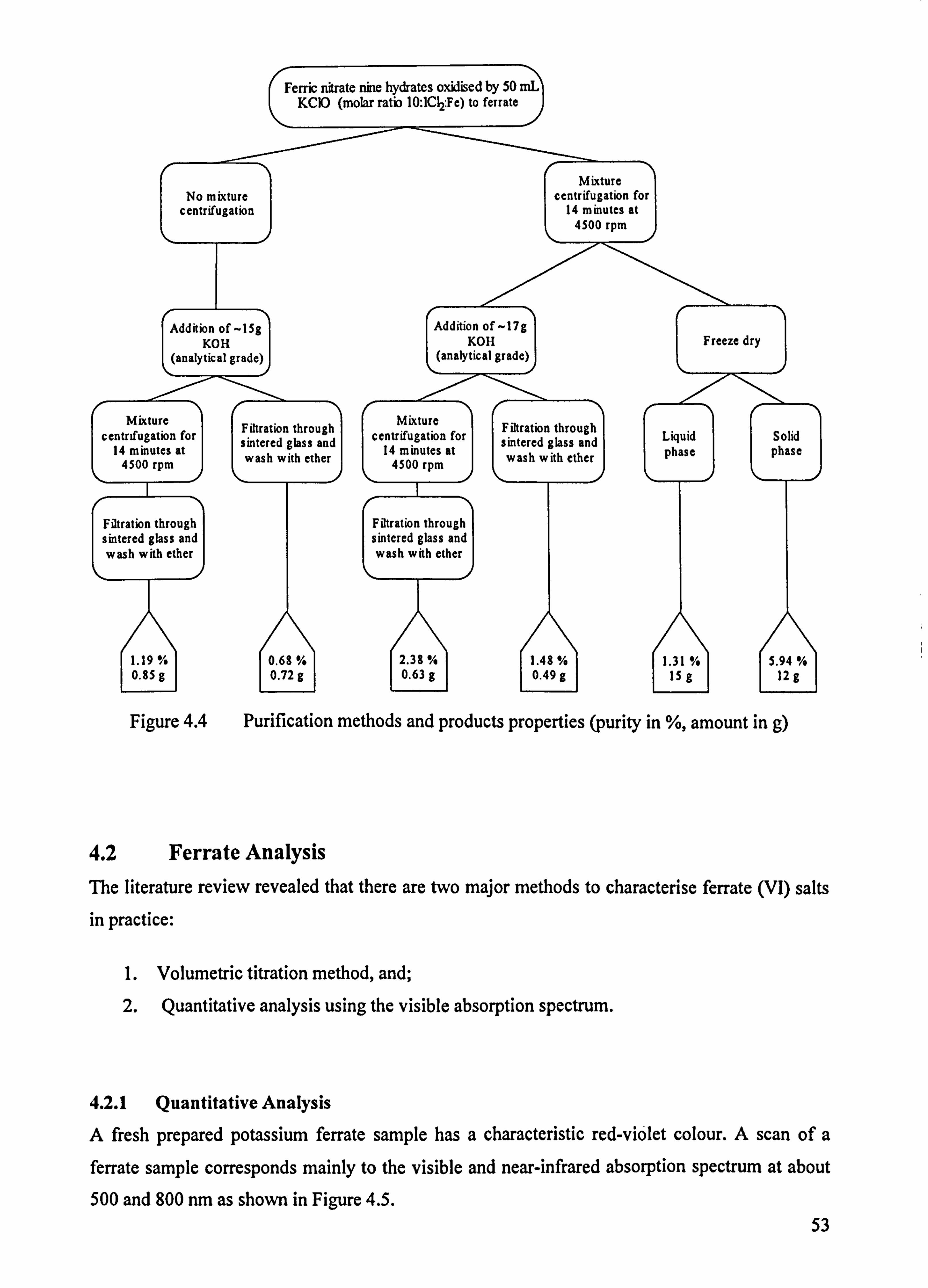
Ferric nitrate nine hydrates oxidised by 50 mL KCIO (molar ratio 10: 1CI2: Fe) to ferrate
Mixture No mixture centrifugation for
centrifugation 14 minutes at 4500 rpm
Addition of -158 Addition of -17g KOH KOH
(analytical grade) (analytical grade)
Mixture centrifugation for
14 minutes at 4500 rpm
Filtration through sintered glass and wash with ether
Filtration through sintered glass and wash with ether
Mixture centrifugation for
14 minutes at 4500 rpm
Filtration through sintered glass and wash with ether
Freeze dry
Filtration through Liquid Solid sintered glass and
phase phase wash with ether
1.19% 0.85 g
0.68% 0.72 g
2.38% 0.63 g
1.48% 0.49 g
1.31'/0 15 g
5.94 % 12 g
Figure 4.4 Purification m ethods and products properties (purity in %, amou nt in g)
4.2 Ferrate Analysis
The literature review revealed that there are two major methods to characterise ferrate (VI) salts in practice:
1. Volumetric titration method, and; 2. Quantitative analysis using the visible absorption spectrum.
4.2.1 Quantitative Analysis
A fresh prepared potassium ferrate sample has a characteristic red-violet colour. A scan of a
ferrate sample corresponds mainly to the visible and near-infrared absorption spectrum at about
500 and 800 nm as shown in Figure 4.5. 53

2.5
1.5 ä.
2.0
e 1.0
0.5
0.0 i
375 400 425 450 475 500 525 550 575 600 625 650 675 700 725 750 775 800 825 850 875 900
Wavelength (nm)
Figure 4.5 UV-Vis spectrum of potassium ferrate (VI)
The region below 390 nm is not shown due to strong hydroxide interference. The data obtained fits well with the published spectra with a peak at 505 nm (Carr, 1981) and two minima at 390
and 675 nm (Neveux, 1994).
Among a range of emission/luminescence spectroscopy methods for the characterisation of ferrate (VI), the infrared (IR) spectroscopy has attracted more attention as it can be used to
determine the potassium ferrate either quantitatively or qualitatively (Griffith, 1966).
For the quantitative analysis of ferrate salts, ferrate's purity is determined at the maximum of the
ferrate peak of 505 nm, using a molar absorption coefficient, e is 1100 M'' cm- ' (Read et at, 1998); various values for this coefficient have been reported in the literature (Wood, 1958; Carr, 1981).
The molar absorption coefficient can be calculated, using a standard ferrate solution with a range
of concentrations; a calibration curve can be made and thus the ferrate concentration can be
measured. This method is simple to carry out and there is no dangerous waste produced.
54
4.2.2 Volumetric Titration Method
The volumetric titration method includes the chromite titration method, the total iron titration
method and the arsenite test. All the methods are addressed in detail as follows in Sections
4.2.2.1,4.2.2.2, and 4.2.2.3.
Volumetric titration analysis can determine the ferrate accurately. However, considering that the
rate of decomposition of acidic ferrate is rapid, a buffer solution is required to maintain the pH of
the ferrate sample at values greater than 8, which will give more reliable results.
4.2.2.1 Chromite Titration Method
Excess chromium (III) is oxidised to chromium (VI) by ferrate in a strong sodium hydroxide
solution, as Equation 4.7 shows. The solution is then acidified with the addition of sulphuric and
phosphoric acids and titrated with ferrous ammonium sulfate using sulphonate solution as an indicator to find the amount of chromium (VI) formed. The end point of the titration is shown as
a change from purple to light green (Schreyer et al., 1950a).
Cr+3 (OH)a" + Fe "'Oä Z+3 H2O -º Fe+3 (OH)3 (H20)3 + Cr"6 04 2+ OH- Equation 4.7
However, the samples wastes need to be stored and treated specifically owing to the existence of
residual chromite in the wastes. The disposal of such wastes should follow the standard laboratory safety and health procedures. Therefore, a more green method for determining the ferrate concentration should be adopted.
4.2.2.2 Total Iron Titration Method (APRA, 1995)
This method is based on the principle that iron will liberate free iodine from potassium iodide
solutions at acidic conditions. The liberated iodine is then titrated with a standard solution of sodium thiosulfate with starch as an indicator.
However, the measurements of ferrate concentrations are biased because the iodide ion can reduce both ferrate (VI) and possible co-existing ferric (III) ions to the ferrous (II) ions. Therefore, a more suitable method for determining the ferrate concentration should be adopted.
55

4.2.2.3 Arsenite Test
Excess of arsenate is oxidised to arsenite by ferrate in a strong sodium hydroxide solution, as
equation 4.8 shows. The solution is then acidified with the addition of concentrated hydrochloric
acid.
The remaining arsenate is back titrated using a bromate or cerate solution and methyl orange as
an indicator, while the solution is still hot. The end point of the titration is shown as a change from golden yellow to green yellow (Schreyer et al., 1950).
2 Fe04 2+ 3 AsOs 3+ 11 H2O --º 2 Fe(OH)3.3(H2O) +3 As04-3+ 40H- Equation 4.8
However, one more as before with chromate titration method, the samples wastes need to be
stored and treated specifically owing to the existence of residual arsenite-bromate/arsenite-cerate in the wastes.
The disposal of such wastes should follow the standard laboratory safety and health procedures.
Therefore, a more environmental friendly method for determining the ferrate concentration
should be adopted.
4.3 Summary
Potassium ferrate has to be prepared prior to the evaluation of it as oxidant, coagulant, and disinfectant. Potassium ferrate was prepared using the wet chlorination method, which involves
the oxidation of ferric nitrate nonahydrate to form ferrate (VI) solution. Since the ferrate
solutions are unstable, it is vital to prepare a solid product for use in practice.
Due to its limited solubility in potassium hydroxide, potassium ferrate can be isolated from its
aqueous solution through a precipitation procedure. Once ferrate has been isolated, it has to be
purified from a range of contaminants, mainly alkali metal hydroxides, chlorides and ferric
oxide, which cause decomposition of ferrate to ferric oxide.
For a successful ferrate synthesis, several parameters have to be considered, such as the purity of
raw materials (analytical/technical grade, type of ferric salt, hypochlorite concentration), the
preparation conditions (reaction time, temperature), and the purification method used.
56

However, even with all these requirements satisfied, the characteristics of potassium ferrate may
still vary. Therefore, the preparation steps and conditions need to be strictly controlled.
Following a systematic series of ferrate preparations, solid ferrate samples (6 per cent as ferrate)
were consistently produced in the laboratory and they were subsequently used for water and
wastewater treatment in laboratory scale.
57
bfýhee bt
This Chapter presents in detail the methods of experiments and analytical procedures that were
used to carry out the study. In section 5.1, all the jar test procedures are given in terms of the
treatment purposes such as coagulation, disinfection and sludge production (Imhoff cone). In
Section 5.2, the procedures used for chemical analysis of iron, aluminium and chlorine
concentrations are presented in detail.
Finally, in Section 5.3, the methods of analysing water quality parameters are detailed including
physical (turbidity, colour, total suspended solids), chemical and biochemical (biological and
chemical oxygen demand) and biological characteristics (total and faecal coliform).
5.1 Jar Tests
The jar test consists of placing several samples of raw water in a series of one-litre beakers (each
with a variable speed stirrer) and stirring in a manner simulating that of a water treatment plant.
Varying dosages of coagulants and other chemicals used in the full-scale process are added to
each beaker. Three modified jar tests (disinfection, coagulation, and sludge production) are
applied based on the investigation purpose and these are addressed in detail as follows.
5.1.1 Modified Jar Tests for Disinfection Performance Evaluation
These jar tests were modified accordingly in order to assess the disinfection performance of
sodium hypochlorite and potassium ferrate. The several samples of raw water were placed in a
series of tall* one-litre beakers. The effectiveness of the disinfectants depends upon applied dose,
disinfection pH and the contact time. The procedure for carrying out the modified jar tests for
disinfection performance evaluation is as follows:
Physical beaker dimensions: 180 mm in height and 95 mm in diameter 58

1. Place IL of the raw water in each of the six beakers and place in positions the stirrers;
2. Commence stirring at 400 rpm;
3. Add the appropriate amount of acid or alkali for pH adjustment;
4. Add the appropriate amount of disinfectant to each beaker at the same time;
5. Stir for one minute at 300 rpm;
6. Turn the stirrer off and take out the paddles;
7. Leave for different contact times of 10,20 and 30 minutes respectively, and;
8. Filter 10 mL of the sample through a glass microfibre filter for turbidity reduction and
test for any chemical concentrations required such as chlorine residual and chlorine
demand.
5.1.2 Modified Jar Tests for Coagulation Performance Evaluation
These jar tests were modified accordingly in order to assess the coagulation performance of
aluminium sulphate (AS), ferric sulphate (FS) and potassium ferrate (FR). Several samples of the
raw water were placed in a series of tails one-litre beakers. The effectiveness of the coagulants
depends upon the applied dose and coagulation pH.
After an appropriate period of mixing and coagulation, stirring was stopped, and the floc formed
was allowed to settle for a specified time. The clarity of the supernatant was then used to
evaluate the optimum chemical dosages. The procedure for carrying out the modified jar test for
coagulation is then as follows:
1. Place 1L of the raw water in each of the six beakers and place in positions the stirrers;
2. Commence stirring at 400 rpm;
3. Add the appropriate amount of acid or alkali for pH adjustment;
4. Add the appropriate amount of coagulant to each beaker at the same time;
5. Stir for one minute at 400 rpm;
6. Stir for 20 minutes at 35 rpm;
7. Turn the stirrer off and take out the paddles;
8. Leave for 60 minutes; 9. Take a pH measurement and decant off 15-20 mL sample for turbidity reading, and;
10. Filter 100 mL of the sample through a 0.45 µm filter paper for colour measurement and
test for any chemical concentrations required.
59

5.1.3 Modified Jar Tests for Sludge Production Evaluation (Imhoff Cone)
These jar tests are modified accordingly in order to assess both coagulation performance and
sludge production of AS, FS, and FR. Several samples of raw water are placed in one-litre
Imhoff cone, as shown in Figure 5.1.
After an appropriate period of mixing and coagulation, stirring is stopped, and the floc formed is
allowed to settle for a specified time. The clarity of the supernatant and the sludge volume is then
used to evaluate the optimum chemical dosages.
The procedure for carrying out the modified jar test for sludge production. evaluation is then as follows:
1. Place IL of the raw water in the Imhoff cone and place in position the stirrer;
2. Commence stirring at 400 rpm; 3. Add the appropriate amount of acid or alkali for pH adjustment;
4. Add the appropriate amount of coagulant to the Imhoff cone at the same time;
5. Stir for one minute at 400 rpm; 6. Stir for 20 minutes at 35 rpm;
7. Turn the stirrer off and take out the paddle; 8. Leave for 60 minutes and decant off 15-20 mL sample for turbidity reading every
minute for the first 5 minutes and then every 10 minutes till the end of the sedimentation time, and;
9. Read the graduated scale on the Imhoff cone at the top of the solids layer as mL/L settleable matter and filter the solids layer through a weighed standard glass fibre filter (Whatman GF/C filter) for total suspended solids measurement.
60

Imhoff cone
idle
filter holder
Figure 5.1 Imhoff apparatus
5.2 Residual Chemical Analysis
In water industry, depending on the primary source of water to be treated such as river water or
wastewater, and the level of treatment required, different chemical concentrations are targeted for
analysis. The residual chlorine, iron, and aluminium were analysed used the following methods
as detailed in sections 5.2.1,5.2.2, and 5.2.3 respectively.
61

5.2.1 Residual Chlorine Analysis
A colourimetric method was used to determine chlorine residual and chlorine demand during
disinfection performance evaluation. Palintest DPD (N, N-diethyl-p-phenylene-diamine) tablets'
are added in 10 ml of solution free of turbidity (prior filtered through a glass microfibre filter of
0.26mm thickness).
Once the colour is developed, pinkish colour, the absorbance (ABS) in cm'' of the solution is
measured at a wavelength of 520 nm, which may vary slightly depending on the model of
spectrometer used.
From a standard solution (100 mg/L as chlorine), five samples were produced with
concentrations of 0.5,1,2,3 and 4 mg/L - this range of concentrations can be detected from the instrument (0.5-5 mg/L).
Calcium carbonate solution (50 mg/L) was used to make up the standard solutions, in order to keep the pH in between the working range from 4 to 10 of the DPD tablets and avoiding dilution
of the prepared standards.
The procedure for carrying out the chlorine calibration curve is then as follows:
1. Take a pH measurement- pH should be in the working DPD tablets range of 4-10; 2. Add DPD tablets no. 1 and no. 3 to 10 mL sample; 3. Wait till colour develops, and; 4. Measure absorbance at a wavelength of 514 nm2-
Having measured the absorbances of known solutions, a calibration graph of concentration
against absorbance is plotted, as Figure 5.2 shows. The equation of the best-fit line is used to
calculate chlorine concentration of unknown samples, based on their absorbance readings.
' DPD tablets are provided by PALINTEST. The working pH range of a DPD tablet is 4-10 and the test range is 0.50 mg/L as chlorine. The tablets are applied in 10 mL samples prior filtered through glass microfibre filters to remove any turbidity that could interfere in photo-spectrophotometer reading. 2 The standard solution with the highest concentration (4 mg/L as chlorine) is scanned for its highest peak. The wavelength where the highest peak occurs, it is used for the subsequent chlorine measurements.
62

5
4
E C Ü3 CO)
C
b2 C
O U
1
R 0.9896 "
II i
Abs
Figure 5.2 Chlorine calibration curve at a wavelength of 514 nm
The equation of the best-fit line is y=44.586x-0.2185, where x and y stand respectively for
absorbance and concentration. The spectrometer is capable to detect only concentrations in the
range of 0.5 to 5 mg/L as chlorine, therefore in case of any solution, which fall out of the
working range has to be diluted before measuring its absorbance.
5.2.2 Residual Iron Analysis
A colourimetric method was used in the study to analyse residual iron concentration and is
addressed in detail as follows. Iron is brought into solution, reduced to the ferrous state by
boiling with acid and hydroxylamine and treated with phenanthroline at pH 3.2 to 3.3, to form an
orange-red complex. The intensity of the colour is independent of pH in the range 2 to 9. The
complex is very stable and the colour intensity does not change appreciably over long periods of
time. Beer's law is obeyed.
From a standard solution (100 mg/L as iron), eight samples were produced with concentrations
of 0.075,0.225,0.45,0.6,1.5,3,4.5 and 6 mg/L - this range of concentrations can be detected
from the instrument (0.05-6 mg/L).
63
0 0 0.01 0.02 0.03 0.04 0.05 0.06 0.07 0.08 0.09 0.1

The iron must be in the ferrous state, and hence a reducing agent, hydroxylamine, was used to
reduce any ferric ion that was present, as Equation 5.1 shows. The pH is adjusted to a value between 6 and 9 by addition of ammonia or sodium acetate.
2 Fe 3+ +2 NH2OH +2 OR --º 2 Fe 2+ + N2 +4 H2O Equation 5.1
The procedure for carrying out the chlorine calibration curve is then as follows:
1. Add hydroxylamine, phenanthroline and acetate to all samples; 2. Take a pH measurement - pH should be in the working range of 6 to 9;
3. Allow solutions to stand for 10 minutes with occasional shaking of the flasks, and;
4. Measure absorbance at a wavelength of 510 nm.
Having measured the absorbances of known solutions, a calibration graph of concentration
against absorbance is plotted, as Figure 5.3 shows. The equation of the best-fit line is used to
calculate iron concentration of unknown samples, based on their absorbance readings.
7
6
E5
c
04 w Co C O
c
Cc 02 U
1
y=5.1966x - 0.0817 R2 = 0.9999
.. Y... __.. _.. _. _ .
I
o+ 0 0.2 0.4 0.6
Absi
0.8 1 1.2
Figure 5.3 Iron calibration at a wavelength of 510 nm
The equation of the best-fit line is y=5.1966x-0.0817, where x and y stand respectively for
absorbance and concentration. The spectrometer is capable to detect only concentrations in the
range of 0.05 to 6 mg/L as iron, therefore in case of any solution, which fall out of the working
range has to be diluted before measuring its absorbance. 64

5.2.3 Residual Aluminium Analysis
Aluminium concentrations can be detected by atomic absorption spectrometric (AAS) and
inductively coupled plasma (ICP) methods. However, the Eriochrome cyanine R colourimetric
method provides a means for estimating aluminium with simpler instrumentation. With working
dye reagent Eriochrome cyanine R, dilute aluminium solutions buffered to a pH of 6.0 produce a
red to pink complex that exhibits maximum absorption at a wavelength of 535 nm.
From a standard solution (100 mg/L as aluminium), five samples were produced with
concentrations of 0.05,0.1,0.15,0.2,0.25 and 0.3 mg/L - this range of concentrations can be
detected from the instrument (0.05-0.35 mg/L). The interference caused by even small amounts
of alkalinity is removed by acidifying the sample at a pH 2. The interference of iron and
manganese, two elements often found in water, is eliminated by the addition of ascorbic acid.
The procedure for carrying out the chlorine calibration curve is then as follows:
1. Acidify the sample and buffer it to a pH 6.0;
2. Add the working dye reagent and mix;
3. Allow solutions to stand for 5-10 minutes, and; 4. Measure absorbance at a wavelength of 535 nm.
Having measured the absorbance of known solutions, a calibration graph of concentration against
absorbance is plotted, as Figure 5.4 shows. The equation of the best-fit line is used to calculate
aluminium concentration of unknown samples, based on their absorbance readings.
0.3:
0.;
a 0.2 c
l0
C 0
o. 1 C 0 0 0 0.
0.0
Figure 5.4 Aluminium calibration at a wavelength of 535 nm 65
0 0.1 0.2 0.3 0.4 0.5 0.6 0.7 0.8 0.9
Abs
The equation of the best-fit line is y=0.3627x+0.0032, where x and y stand respectively for
absorbance and concentration. The spectrometer is capable to detect only concentrations in the
range of 0.05 to 0.35 mg/L as aluminium, therefore in case of any solution, which fall out of the
working range has to be diluted before measuring its absorbance.
5.3 Water Quality Parameters Analysis An understanding of the nature of water sample is essential in the design and operation of treatment, and disposal facilities. To promote this understanding, physical, chemical and biological characteristics of both water and wastewater samples are presented in detail as follows.
5.3.1 Physical Characteristics
The most important physical characteristics of water and wastewater is its turbidity, colour and total suspended solids content, which is composed of floating matter, settleable matter, colloidal matter, and matter in solution.
5.3.1.1 Turbidity
Turbidity is a measure of the extent to which suspended matter in water, either absorbs or scatters radiant light energy impinging upon the suspension. Turbidity measurements are done
using photometers. A beam of light from a source produced by a standardised electric bulb is
passed through a sample vial. The sample scatters the light that impinges upon it.
The scattered light is then measured by putting the photometer at right angles from the original direction of the light generated by the light source. This measurement of light scattered at a 90- degree angle is called nephelometry. The unit of turbidity in nephelometry is the Nephelometric
turbidity unit (NTU).
The colour is determined by the photometric method using a Jenway turbidimeter (model 6035).
This model operates over the range of 0.00 to 199.99 NTU with a resolution of 0.1. For optimum
performance calibration should be carried out at the beginning and end of every sample batch.
66

5.3.1.2 Colour (Vis-abs at 400 nm)
Colour in water may result from the presence of natural metallic ions (iron and manganese), humus and peat materials, and industrial wastes. To determine colour by currently accepted
methods (visual comparison method and spectrophotometric method), turbidity must be removed before analysis by either filtration or centrifugation.
Prior to colour measurement, a membrane filter with pore size of 0.45 µm filter paper is used for
turbidity reduction - the pore size 0.45µm has been prescribed as mandatory for determination of
spectral absorption (ISO, 1994). The EU drinking water standard prescribes simple filtration
though glass fibre filter before colour determination (EEC Council Directive 79/869).
The colour is determined by the spectrophotometric method using a Unicam Helios a UV-visible
spectrometer. The absorbance is measured at a selected wavelength of 400 nm, as it was found
that other wavelengths may cause large discrepancies between spectrophotometric and visual
colour determination (Akesson and Hongve, 1996).
5.3.1.3 UV-abs at 254 nm
Organic compounds that are aromatic or that have conjugated double bonds absorb light in the ultraviolet (UV) wavelength region (<400 nm). UV absorbance is a good technique for
measuring the presence of naturally occurring organic matter (Edzwald et al., 1985), such as humic substances, because they contain aromatic moieties and are the dominant form of organic matter in natural waters.
Prior to UV measurement, the sample is passed through a membrane filter with pore size of 0.45
µm for turbidity reduction. The colour is then determined by the spectrophotometric method
using a Unicam Helios a UV-visible spectrometer setup at a wavelength of 254 nm.
5.3.1.4 Total Suspended Solids
This is a measure of the total particulate matter content of a waste. The nature of the TSS is
likely to vary considerably depending on the nature of the waste. A well-mixed sample of 100
mL is filtered through a weighed standard glass fibre filter (Whatman GF/C filter) and the
residue retained on the filter is dried to a constant weight at 103 to 105° C overnight. The
increase in weight of the filter represented the total suspended solids present in the sample.
67

5.3.2 Chemical and Microbiological Characteristics
There are many compounds and microorganisms present in both water and wastewater, which are
capable of causing the pollution of a watercourse. According to Horan, the components comprise
a water sample can be defined in terms of three broad categories, namely:
1. Organic material - all the organic components have in common the possession of at least
one carbon atom , which may be oxidised both chemically and biologically to yield
carbon dioxide. Oxidation reactions may be carried out both microbially and by use of
chemical oxidising agents. For biological oxidation, the biological oxygen demand
(BOD) test can be used, whereas for chemical oxidation, the chemical oxidation demand
(COD) test can be employed. Both these tests allow a gross determination of the
pollution potential present in a sample; 2. Inorganic material - the inorganic material that pose the threat of pollution are limited to
individual compounds. The most important of these compounds are nitrogen and
phosphorus, which are most likely to prove troublesome especially, and;
3. Microbial content - the microbial content of a watercourse has a wide variety of
microorganisms including viruses, bacteria, fungi, protozoa and nematodes. The aim in
the microbiological examination of a water is to detect the presence of pathogenic microorganisms which would constitute a danger to human health through contact with the contaminated water.
5.3.2.1 Biochemical Oxygen Demand (BOD)
The most widely used parameter of organic pollution applied to both wastewater and surface
water is the 5 day BOD. This determination involves the measurement of dissolved oxygen used by microorganisms in the biochemical oxidation of organic matter.
The BOD test though has two major disadvantages: (a) it takes 5 days to obtain the standard test
result, and (b) the results can be affected by the process of nitrification. Nitrification consumes
significant amounts of oxygen and generates protons (H+ ions), increasing the acidity (pH) of the
waste. Nitrification originates from the degradation of proteins to release ammonia.
The biochemical oxygen demand (BOD) test is carried out as follows: measured amounts of a
wastewater (suitably diluted with a prepared water) are placed in 280 mL BOD bottles. The
prepared water is (a) saturated with dissolved oxygen, and (b) it contains nutrients and a buffer. 68
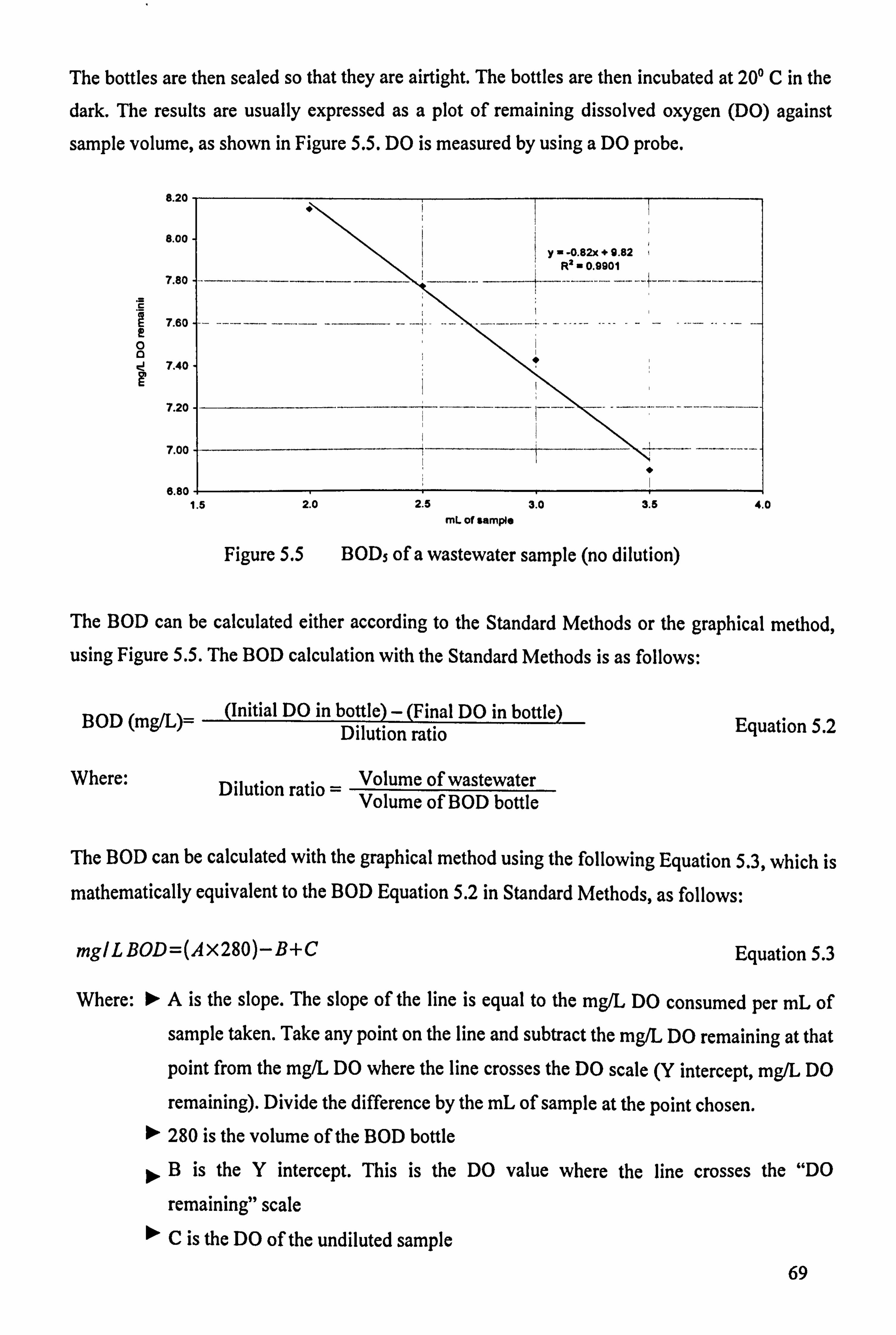
The bottles are then sealed so that they are airtight. The bottles are then incubated at 20° C in the
dark. The results are usually expressed as a plot of remaining dissolved oxygen (DO) against
sample volume, as shown in Figure 5.5. DO is measured by using a DO probe.
8.20
8.00
7.80
7.60
0 7.40
7.20
7.00
8.80
ii
r '-0.82X + 9.92 , R=0.9901
.
1.5 2.0 2.5 3.0 3.5 f. 0
mL of sample
Figure 5.5 BOD5 of a wastewater sample (no dilution)
The BOD can be calculated either according to the Standard Methods or the graphical method,
using Figure 5.5. The BOD calculation with the Standard Methods is as follows:
BOD (mg/L)= (Initial DO in bottle) - (Final DO in bottle) Dilution ratio
Where: Dilution ratio = Volume of wastewater Volume of BOD bottle
Equation 5.2
The BOD can be calculated with the graphical method using the following Equation 5.3, which is
mathematically equivalent to the BOD Equation 5.2 in Standard Methods, as follows:
mglL BOD=(AX280)-B+C Equation 5.3
Where: ºA is the slope. The slope of the line is equal to the mg/L DO consumed per mL of sample taken. Take any point on the line and subtract the mg/L DO remaining at that
point from the mg/L DO where the line crosses the DO scale (Y intercept, mg/L DO
remaining). Divide the difference by the mL of sample at the point chosen. º 280 is the volume of the BOD bottle
00. B is the Y intercept. This is the DO value where the line crosses the "DO
remaining" scale C is the DO of the undiluted sample
69

Equation 5.3 can be applied in Figure 5.5 for the calculation of BOD5, where slope = 0.82 mg/L
per mL, Y inter = 9.82 mg/L, and sample DO = 0.38 mg/L.
Therefore: (0.82x280)-9.82+0.38=220.16mg/LBOD
The COD of a waste is, in general, higher than the BOD because more compounds can be
chemically oxidised than can be biologically oxidised. The COD of the sample wastewater sample that was used for BOD measurement, it had a COD value of 503 mg/L.
It is possible to correlate COD with BOD. This is very useful because the COD can be
determined in three hours, compared with five days for the BOD. Once correlation has been
established, COD measurements can be used to good advantage for treatment plant control and
operation. The procedure for carrying out the correlation of BOD with COD is as follows:
1. Take a fresh sample of wastewater;
2. Make five dilutions of the sample 0,1.3,2,4 and 10 times, and; 3. Calculate the COD and BODS.
Having measured the COD and BOD5 of all dilutions, a calibration graph of BODE against COD is plotted, as Figure 5.6 shows. The equation of the best-fit line is used to calculate BOD
concentration of unknown samples, based on their COD readings.
550
500
450
400
350
ý, 300 E
0 250 U
200
150
100
50
0
i
Direct COD -- y= . 7152x+127.11-----
R2 = 0.9985
0 25 50 75 100 125 150 175 200 225
BOD (mg/L)
Figure 5.6 Correlation of BOD with COD 70

The equation of the best-fit line is y=1.7152x+127.11, where x and y stand respectively for the
concentrations of BOD and COD. It is possible to correlate COD with BOD for other types of
waters such river water and lake water, however low BOD values of 2-6 mg/L have proved not to
give such a strong correlation as wastewater samples do.
5.3.2.2 Chemical Oxygen Demand (COD)
In this test, strong chemical reagents are used to oxidise the waste. The COD test predicts the
oxygen requirement of the effluent. The measurement of COD is assumes all organic
compounds, with a few exemptions, can be oxidised by the action of strong oxidising agents
under acid conditions.
The dichromate reactor digestion method test as developed by HACH Company (Colorado,
USA) is used. There are two types of COD vials that can be used: a) mercury free, and b) with
mercury.
The use of free mercury COD vials gave inconsistent readings. One possible explanation could
be the chloride present in the ferrate, since ferrate is prepared after the modified chlorine method.
The interference can be eliminated by the use of mercury COD vials, because the mercury ion
combines with the chloride ions and precipitates out (AWWA, 1995).
Even if mercury COD vials were used, inconsistent results continued to occur. A possible reason
could be organic compounds, particularly low molecular weight fatty acids that are not oxidised
unless a catalyst is present such as silver ion (AWWA, 1995).
It is possible to correlate COD with UV absorbance at a wavelength of 254 nm (Mrkva, 1983).
This is very useful because the UV absorbance at 254 nm can be determined immediately,
compared with 3 hours for the COD.
Correlation is a sufficiently precise method permitting a simple indication of the organic
pollution extent (Dobbs et al., 1972). Once correlation has been established, UV absorbance
measurements at 254 nm can be used to good advantage for treatment plant control and
operation.
71

The procedure for carrying out the correlation of UV absorbance at 254 nm with COD for a
wastewater is as follows:
1. Take a fresh sample of wastewater;
2. Make seven dilutions of the sample 0,2,4,6,8,10 and 12 times;
3. Measure filtered (0.45 µm filter paper) and unfiltered COD;
4. Measure UV absorbance at 254 nm prior to filtration through a 0.45 µm filter paper.
Having measured both filtered and unfiltered COD, and UV absorbance at 254 nm of all
dilutions of wastewater, a calibration graph of UV absorbance at 254 nm against
filtered/unfiltered COD is plotted, as Figure 5.7 shows.
700
600
500
400 O O
300
200
100
f COD Unfiltered COD Filtered
Filtered COD y= 270.47x + 108.08
R2 = 0.9968'
Unfiltered COD y 1502.6x + 100.45
R2=0.9868
0i 0 0.05
Figure 5.7
i0
200
150
0 0
100 LL,
50
0 i 0.1 0.15 0.2 0.25 0.3 0.35
UV Absorbance at 254 nm
Correlation of UV absorbance at 254 nm with filtered COD
The equation of the best-fit line for filtered COD is y=270.47x+108.08, and for unfiltered COD
is y=1502.6x+100.45, where x and y stand respectively for UV absorbance at 254 nm and
filtered/unfiltered COD. The equation of the best-fit line is used to calculate COD concentration
of unknown samples, based on their UV absorbance at 254 nm readings.
72
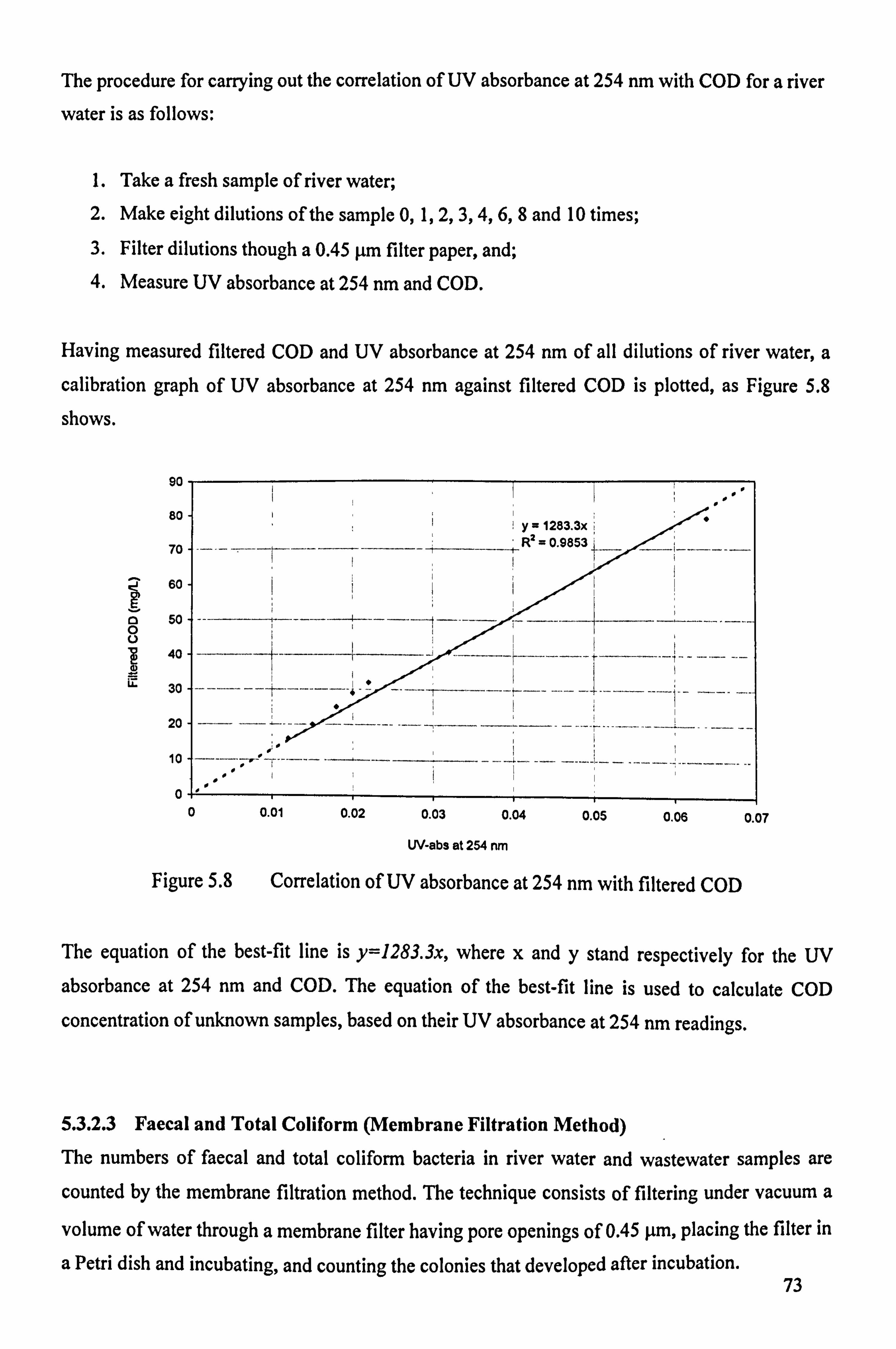
The procedure for carrying out the correlation of UV absorbance at 254 nm with COD for a river water is as follows:
1. Take a fresh sample of river water; 2. Make eight dilutions of the sample 0,1,2,3,4,6,8 and 10 times;
3. Filter dilutions though a 0.45 µm filter paper, and; 4. Measure UV absorbance at 254 nm and COD.
Having measured filtered COD and UV absorbance at 254 nm of all dilutions of river water, a
calibration graph of UV absorbance at 254 nm against filtered COD is plotted, as Figure 5.8
shows.
90
80
70
60
0 50 0 U
40
LL 30
20
10
0
y= 1283.3x
-- --- -- - ----- ------ ----- + R2 = 0.9853-i_
-- --
i
----------
-- --- -- ---- --- ----- - ------
i
0 0.01 0.02 0.03 0.04 0.05 0.06 0.07
UV-abs at 254 nm
Figure 5.8 Correlation of UV absorbance at 254 nm with filtered COD
The equation of the best-fit line is y=1283.3x, where x and y stand respectively for the UV
absorbance at 254 nm and COD. The equation of the best-fit line is used to calculate COD
concentration of unknown samples, based on their UV absorbance at 254 nm readings.
5.3.2.3 Faecal and Total Coliform (Membrane Filtration Method)
The numbers of faecal and total coliform bacteria in river water and wastewater samples are
counted by the membrane filtration method. The technique consists of filtering under vacuum a
volume of water through a membrane filter having pore openings of 0.45 µm, placing the filter in
a Petri dish and incubating, and counting the colonies that developed after incubation. 73

The 0.45 µm opening retains the bacteria on the filter. The volume of sample to be filtered
depends on the anticipated bacterial density. Sample volumes that yield plate count of 20 to 80
colonies on the Petri dish is considered more valid. The standard volume filtered in potable water analysis is 100 mL.
If the anticipated concentration is high requiring a smaller volume of sample, the sample must be diluted to dispersed the bacteria uniformly. The dispersion will ensure a good spread of the
colonies on the plate for easier counting.
The culture medium is prepared by putting an absorbent pad on a Petri dish and pipetting enough lauryl sulphate broth into the pad. After filtration, the membrane is removed by forceps and
placed directly on the pad.
The culture is then incubated at 35 f 0.5°C in the case of the coliform group and at 44.5 ± 0.5°C
in the case of the faecal coliforms - thermotolerant coliform (assumed faecal). During incubation, each faecal and total coliform bacteria develops into a visible yellow colony. At the
end of the incubation period of 24 ±2 hours, the number of yellow colonies that developed are counted and reported as number of organisms per 100 mL.
74

Water supplies are usually disinfected. The widespread adoption of disinfection was a major factor in reducing waterborne diseases, and this has been interpreted as the major single factor in
increasing average human life expectancy.
Disinfection is carried out to destroy the harmful microorganisms that cause diseases. It differs
from sterilisation, which implies the destruction of all microorganisms. Sterilisation is not often
practiced in the treatment of water and wastewater.
This chapter details the disinfection and coagulation performance of potassium ferrate in treating
the University of Surrey lake water. In the first part of this Chapter, Section 6.2, the unit process
of disinfection is briefly outlined. There is a short discussion on the methods of disinfection,
factors affecting disinfection performance, and the various disinfectants that have been used. And
then, the disinfection performance with a chlorine based disinfectant and potassium ferrate is
extensively discussed.
In the second part of this Chapter, Section 6.3, the coagulation performance of potassium ferrate
comparing with other coagulants e. g., ferric sulfate (FS) and aluminium sulfate (AS) is reported
and discussed.
6.1 Lake Water
Lakes are ideal for potable water supplies because they are good storage areas and are more
easily controlled, however, there are many problems associated with eutrophication. Algal
blooms and their subsequent metabolic and degradation products often lead to taste and odour
problems which cannot be totally remedied by water treatment processes. The natural process of
eutrophication can be dramatically speeded up through human and animal activity, where excess
nutrients added from recreational activities leads to pollution. 75

Water samples were collected from the upper lake located in the main campus at the University
of Surrey in Guildford. Samples were collected in high density polyethylene (HOPE) jerricans
washed and rinsed with tap water before use. The disinfection process has been applied to a lake
sample, whose characteristics are given in Table 6.1.
Table 6.1 Characteristics of lake water during March-April 2001
Parameter Range Mean Value
pH 7.8-8.0 7.9
Turbidity (NTU) 6.8-61.8 34.3
Total Suspended Solids (mg/100 mL) 3.8-7.8 5.8
Colour as UV-abs at 254 nm (cm') 0.095-0.138 0.117
Colour as Vis-abs at 400 nm (cm-`) 0.009-0.014 0.012
Total Coliform (per 100 mL) 11-21x104 16x104
Faecal Coliform (per 100 mL) 5-25x104 15x104
As it can be seen from Table 6.1, there is variation in the values of the parameters as a result of
weather conditions depending on the season (dry/wet) and of the activity of local wildlife, in this
case ducks/swans, and people who use the lakes for recreational purposes.
6.2 Lake Water Disinfection
Generally, two methods of disinfection are used: chemical and physical. The chemical methods, of course, use chemical agents, and the physical methods use physical means. Historically, the
most widely used chemical agent is chlorine.
Other chemical agents that have been used include ozone, the halogens bromine and iodine and bromine chloride, KMnO4, and many others. The physical means of disinfection that have been
used include ultraviolet light (UV), electron beam, sonification, and heat.
In general, the effect of disinfectants is thought to occur as a result of the damage to cell walls,
alteration of cell permeability, alteration of the protoplasm, and inhibition of enzymatic
activities.
76

6.2.1 Factors Affecting Disinfection
The effectiveness of disinfectants are affected by the following factors: contact time between
disinfectant and the microorganisms, the type and concentration of the disinfectant used, the
quality characteristics of the suspending water, and disinfection pH. Each of these factors is
discussed as follows.
6.2.1.1 Contact Time and Concentration of Disinfectant
It is universal fact that the time needed to kill a given percentage of microorganisms decreases as
the concentration of the disinfectant increases, and the time to kill the same percentage of
microorganisms increases as the concentration of the disinfectant decreases, as shown in Figure
6.1. Therefore, the time to kill and the disinfectant concentration are in inverse ratio to each
other.
I-o-0.5 mg/L -a-1 mg/L -tr- 2 mg/L
100
80
60
d m
40 0
20
0
lime of contact (in minutes)
Figure6.1 Significance of contact time and disinfectant dose on bacteria inactivation (White, 1999)
6.2.1.2 The Quality Characteristics of the Raw Water
In addition to the contact time and the concentration of disinfectant, the nature of the raw water
also affects the effectiveness of a given disinfectant. Extraneous materials in the water such as ferrous, hydrogen sulphide, and nitrates react with applied disinfectant before the disinfectant can do its job of disinfecting. Also, the turbidities of the water reduces disinfectant effectiveness by
shielding the microorganism. Hence, for most effective kills, the water should be free of turbidity
prior to disinfection. 77
0 10 20 30

6.2.1.3 Disinfection pH
The disinfection pH also affects the effectiveness of a given disinfectant. It is a universal fact that
the concentration of disinfectant needed to kill a given percentage of microorganism decreases as
the pH decreases, and the concentration of disinfectant increases as the pH increases. Therefore,
the concentration of disinfectant and pH are in direct ratio to each other.
The disinfection performance will be improved at lower pH, partly due to the fact that acidity itself will damage to the cell walls of bacteria and partly because of lower pH will be favourable
to the formation of more active disinfectant species, for example, free chlorine.
6.2.2 Experimental Set-up
The three parameters that influence the performance of any given disinfectant are pH conditions,
chemical dosage, and contact time. The tests were carried out for all the possible combinations of
these parameters - in every test, one of the three parameters was altered, while the other two
were kept constant.
The experimental conditions are listed as follows:
Disinfection pH - low pH values can improve significant disinfection performance. Three pH values were examined: 3.5,5.5 and 7.5;
Chemical dose -5 chemical doses were examined: 0.5,1,2,3 and 4 mg/L as ion, and; Contact time of -3 disinfection times were tested: 10,20 and 30 minutes.
In this study , the type of the disinfectant used, the optimum dose, pH and contact time were determined by a modified jar test . Six beakers (500 mL in volume) filled with the raw water
were put into the jar test apparatus (Stuart Scientific Flocculator SW1), and disinfectant was dosed in terms of various demand. A blank sample (only pH adjustment and no disinfectant
addition) was used in order to evaluate the pH significance in bacteria inactivation.
Upon the addition of the disinfectant, the desired pH values were adjusted. The samples were
then rapidly mixed at a speed of about 290-300 rpm for a period of 10,20 and 30 minutes
(contact time).
78
After the stirring was stopped, the samples were firstly filtered with a glass microfibre filter (pore
size of 160-250 µm) and then analysed for chlorine residual, chlorine demand, and bacteria
inactivation achieved. The numbers of total coliform and faecal coliform before and after treatment were determined using a membrane filter method (APHA, 1995).
6.2.2.1 Chlorine Residual
A colourimetric method was used to determine chlorine residual and chlorine demand during
disinfection performance evaluation as described in Section 5.2.1. The absorbance of the sample
was measured at the wavelength of 514 nm using a Unicam HeXios a spectrometer.
6.2.2.2 Chlorine Demand
Chlorine demand in mg/L can be easily calculated, by subtracting chlorine residual from the
equivalent chlorine dose. It is important though that all chlorine determinations should start immediately after sampling, avoiding excessive light and agitation, as the chlorine content of the
samples or solutions, particularly weak solutions, will decrease rapidly.
6.2.2.3 Measurement of Total and Faecal Coliform
In addition to the chemical characterisation of water, it is important that the microbiological constituents be also addressed. Hence, total and faecal coliform are measured before and after disinfection by membrane filtration method described in Section 5.3.2.3.
6.2.3 Disinfectants
The potassium ferrate was evaluated for its disinfection performance comparing with sodium hypochlorite [NaClO]. In the beginning, calcium hypochlorite [Ca(ClO)2] was tried as it contains 70-80 per cent available chlorine.
However, there was some difficulty involved in dissolving it in the water. Sodium hypochlorite
was used instead, which although it contains only 12-17 per cent available chlorine, it was much
easier to dissolve.
79
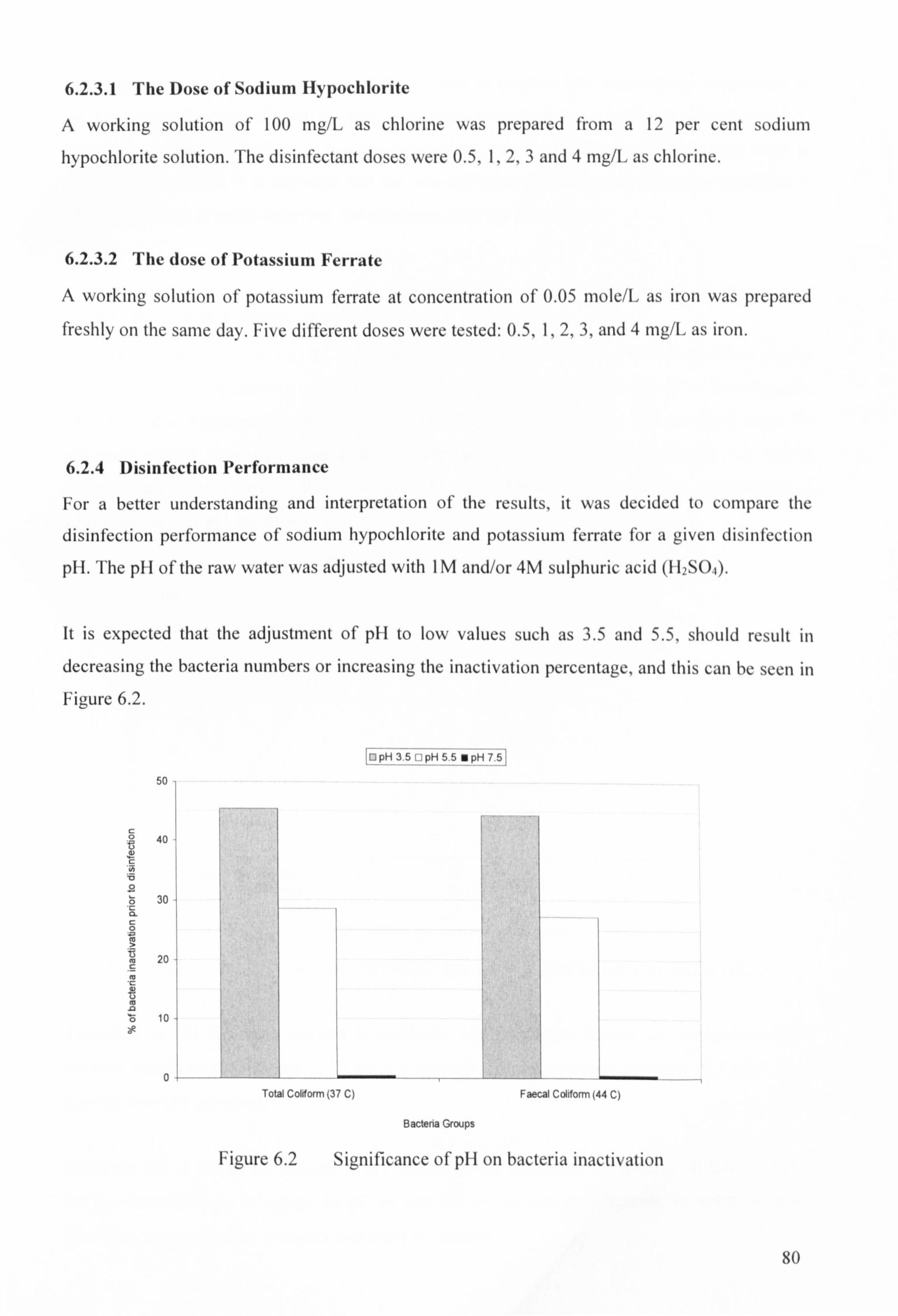
6.2.3.1 The Dose of Sodium Hypochlorite
A working solution of 100 mg/L as chlorine was prepared from a 12 per cent sodium
hypochlorite solution. The disinfectant doses were 0.5,1,2,3 and 4 mg/L as chlorine.
6.2.3.2 The dose of Potassium Ferrate
A working solution of potassium ferrate at concentration of 0.05 mole/L as iron was prepared freshly on the same day. Five different doses were tested: 0.5,1,2,3, and 4 nig/L as iron.
6.2.4 Disinfection Performance
For a better understanding and interpretation of the results, it was decided to compare the
disinfection performance of sodium hypochlorite and potassium ferrate for a given disinfection
pH. The pH of the raw water was adjusted with IM and/or 4M sulphuric acid (I 12SO4).
lt is expected that the adjustment of p1i to low values such as 3.5 and 5.5, should result in
decreasing the bacteria numbers or increasing the inactivation percentage, and this can be seen in
Figure 6.2.
QpH3.5El pH55 apH7.5]
50
c B 40
`c N
V O
ö 30 c CL c 0 a N m
20 c c v Ü
a ö 10 8R
0
Bacteria Groups
Figure 6.2 Significance of pH on bacteria inactivation
80
Total Coliorm (37 C) Faecal Coliform (44 C)

At the lowest pH value of 3.5, almost fifty per cent of bacteria was successfully inactivated. at
pH 5.5, one third of the original bacteria population was inactivated, whilst at a higher pH 7.5,
there was no significant effect on bacteria inactivation, as the pH of raw water was very close to
this value. Therefore, it is expected that the concentration of disinfectant needed to inactivate a
given percentage of microorganism should decrease as the pH decrease.
6.2.4.1 Disinfection Results at pH 3.5
At the lowest pH value of 3.5, the concentration of the disinfectant and the contact time should
decrease significantly due to a number of bacteria have already been inactivated by lowering pH.
Therefore, it is expected that the maximum bacteria inactivation (e. g., 100 per cent) could be
achieved with a minimum disinfectant concentration and contact time. Figure 6.3 shows
disinfection performance of both sodium hypochlorite and potassium ferrate for a contact time of
10 minutes after a pH adjustment at 3.5.
-0-Total Coliform (37 C) -o- Faecal Coliform (44 C)
100
80
60
ao
20
0
i ýI
Raw Water only pH 0.5 1234 adjustment
Concentration of disinfectant (in mgl as Ion)
Figure 6.3 Inactivation rates by NaC1O and K2FeO4 after 10 minutes and at pH 3.5
Therefore, at pH 3.5, both sodium hypochlorite and potassium ferrate can achieve complete
bacteria inactivation (100 per cent) for a minimum disinfectant concentration (0.5 mg/L) and
contact time (10 minutes).
However, pH as low as 3.5 is usually applied only under laboratory conditions - it is not the case
for the water industry to adjust the pH so low just to use less disinfectants, as water treatment
processes are much more complex and more expensive. 81

6.2.4.2 Disinfection Results at pH 5.5
At pH 5.5, it was demonstrated before that the bacteria population present in the raw water can
be reduced to one third of the original one after pH adjustment. As before, it is expected that the
concentration of the disinfectant and the time of contact should decrease due to a number of
bacteria have already been inactivated by pH adjustment. Figures 6.4 and 6.5 show respectively disinfection performance of potassium ferrate and sodium hypochlorite for different contact
times (10,20 and 30 minutes) after a pH adjustment at 5.5.
jtTC (10min) -a-FC (10min) -a-TC (20min) -a-FC (20min) - -TC (30min) -o-FC (30mmn)
100 11 13 Cl 13
80
.Z
60
40
0
20
i!
__.. ______ý. ________. __y, . _. _____. __. _ i_ ... _ i ýý
ýý
i
ii
__...... _. __. L. ___ý_. __..... _.... I. _... _.. ý . _..... _ ..... u_., ý_
0... Raw Water only pH 0.5 123
adjustment
Concentration of potassium ferrate (in mg/L as Ion)
Figure 6.4 Inactivation rates of potassium ferrate at pH 5.5
-f-TC (10min) -d- FC (10min) -a--TC (20min) -o- FC (20min) -. -TC (30min) -0-FC (30min)
100, y0
so
9 a m
ý'- ÖO m c
40 a 's
20
4
Concentration of sodium hypochbrite (in mp/L as ion)
Figure 6.5 Inactivation rates of sodium hypochlorite at pH 5.5
82
0IS Iiiii Raw Water only pH 0.5 1234
adjustment
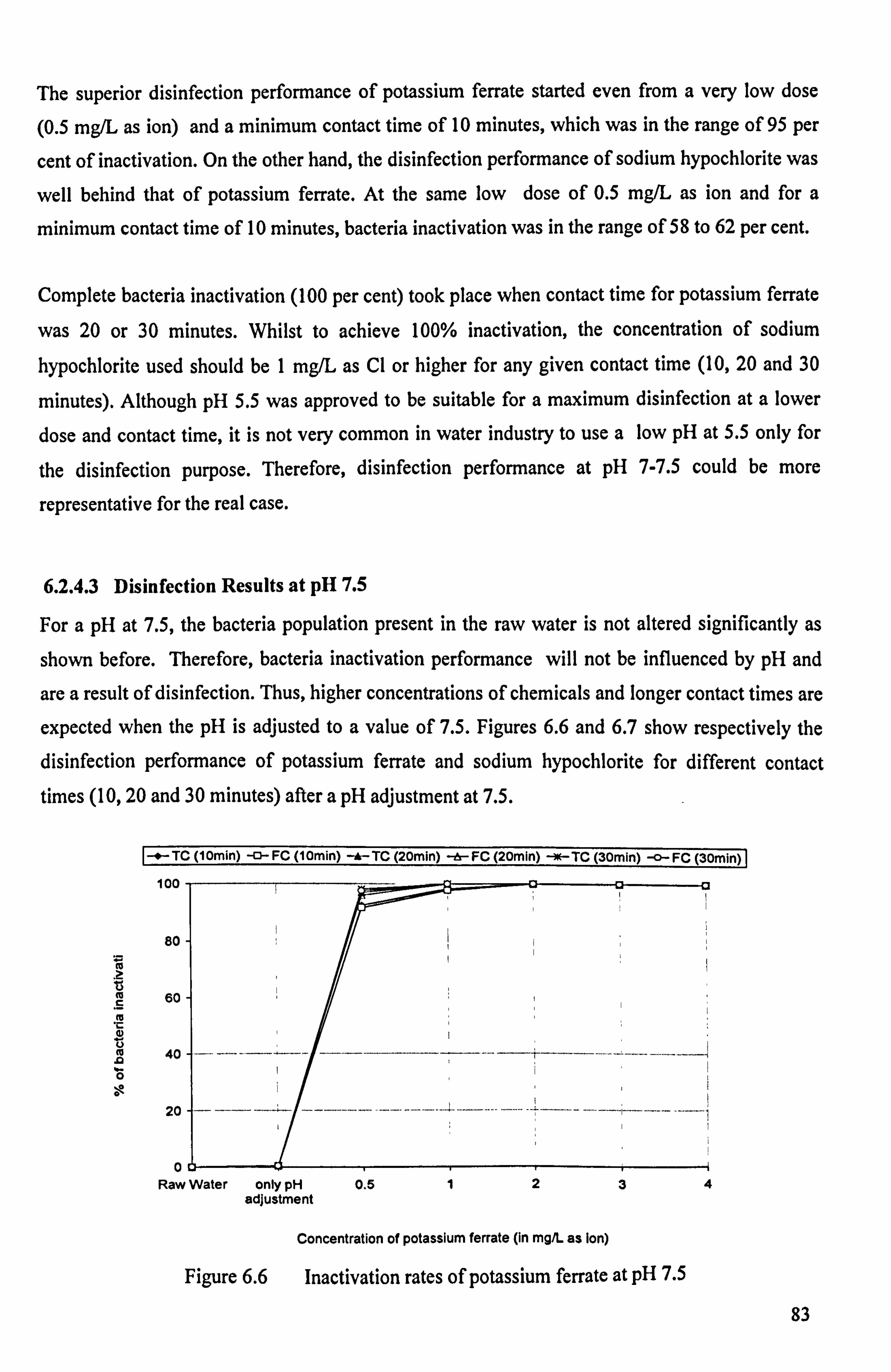
The superior disinfection performance of potassium ferrate started even from a very low dose
(0.5 mg/L as ion) and a minimum contact time of 10 minutes, which was in the range of 95 per
cent of inactivation. On the other hand, the disinfection performance of sodium hypochlorite was
well behind that of potassium ferrate. At the same low dose of 0.5 mg/L as ion and for a
minimum contact time of 10 minutes, bacteria inactivation was in the range of 58 to 62 per cent.
Complete bacteria inactivation (100 per cent) took place when contact time for potassium ferrate
was 20 or 30 minutes. Whilst to achieve 100% inactivation, the concentration of sodium hypochlorite used should be 1 mg/L as Cl or higher for any given contact time (10,20 and 30
minutes). Although pH 5.5 was approved to be suitable for a maximum disinfection at a lower
dose and contact time, it is not very common in water industry to use a low pH at 5.5 only for
the disinfection purpose. Therefore, disinfection performance at pH 7-7.5 could be more
representative for the real case.
6.2.4.3 Disinfection Results at pH 7.5
For a pH at 7.5, the bacteria population present in the raw water is not altered significantly as
shown before. Therefore, bacteria inactivation performance will not be influenced by pH and
are a result of disinfection. Thus, higher concentrations of chemicals and longer contact times are
expected when the pH is adjusted to a value of 7.5. Figures 6.6 and 6.7 show respectively the
disinfection performance of potassium ferrate and sodium hypochlorite for different contact
times (10,20 and 30 minutes) after a pH adjustment at 7.5.
It TC (10min) -o- FC (10min) -e-TC (20min) -6- FC (20min) -*-TC (30min) -0-- FC (30min)
100 -a Dü
80
ii
2 60
d Ü
40
0 0
20
0a-- Raw Water only pH 0.5 1234
adjustment
Concentration of potassium ferrate (in mg/L as ion)
Figure 6.6 Inactivation rates of potassium ferrate at pH 7.5
83

Same as at low pH values, the potassium ferrate can achieve 90% inactivation at a low dose of
0.5 mg/L as ion and a minimum contact time of 10 minutes. The main reason for this could be
that in addition to the odixation activity involved in the process, the potassium ferrate ions were
reduced to form ferric hydroxide, which in turn, entrap a substantial number of bacteria in the
formed flocs and then are removed by sedimentation.
At the same dose of 0.5 mg/L as ion, but for a longer time of contact (30 minutes), potassium ferrate can achieve a 100 per cent bacteria inactivation depending on the characteristics of the
raw water.
Completed bacteria inactivation (100 per cent) was achieved for a potassium ferrate dose of 1
mg/L as ion and contact times of 20 and 30 minutes, except 10 minutes (95+ per cent
disinfection), or when the dose of potassium ferrate was 2 mg/L as ion for any given contact time
(10,20 and 30 minutes).
On the other hand, the disinfection performance of sodium hypochlorite was not as good as
potassium ferrate especially for doses lower than 2 mg/L as ion, as shown in Figure 6.7.
However, completed bacteria inactivation (100 per cent) took place when the dose of sodium hypochlorite was 2 mg/L as ion or higher for any given contact time (10,20 and 30 minutes).
-A-TC (10min) -a--FC (10min) -x-TC (20min) -u-FC (20min) -+-TC (30min) -0-FC (30min)
100
80
O
Z 60 ii
40
ö
20
00 91; Raw Water only pH 0.5 1234
adjustment
Concentration of sodium hypochlorite (in mg/L as ion)
Figure 6.7 Inactivation rates of sodium hypochlorite at pH 7.5
84

6.2.4.4 Chlorine Residuals and Demands
Chlorine residual is expected to be higher for higher doses of sodium hypochlorite depending on
pH, as not all the chlorine available would be consumed for the inactivation of bacteria. It is very important to know the exact amount of chlorine residual present in the treated water. Adequate
levels of chlorine residual are of crucial importance for distribution networks in order to avoid the adverse effects of water contamination.
At low doses of 0.5 and 1 mg/L as ion, there was no chlorine residual to be measured with the
selected method of DPD tablets, as the applied chlorine was immediately consumed by
mircoorganisms most probably.
Chlorine residuals were measurable for applied doses of 2 mg Cl/L and above. The chlorine
residual was dependant not only on the applied dose, but also on the disinfection pH as shown in
Figure 6.8.
3.5
2.5
C `. 2
I-+- pH 3.5 -x- pH 5.5 -6- pH 7.5
3
ýo 0 N d
: i; 1.5 C c 0
L U
0
0.5
2 3 4
Concentration of sodium hypochlorite (in mg/L as ion)
Figure 6.8 Chlorine residuals after a contact time of 10 minutes
At low pH values such as 3.5, sodium hypochlorite did not dissociate almost at all, leaving a
small residual in the treated water. At a pH value of 5.5, sodium hypochlorite dissociated,
leaving reasonable levels of residual in the water.
85

However, at higher pH values such as 7.5, sodium hypochlorite's almost completely dissociated
to OC1', making disinfection less effective. This is partly due to less hypochlorous acid (powerful
disinfectant) will be produced at pH 7.5, and partly less hydrogen ions at pH 7.5 will be
produced, which favours to increase in the disinfection efficiency.
Chlorine demands were measurable for applied doses of 2 mg Cl/L and above. The chlorine demand was dependant not only on the applied dose, but also on the disinfection pH as shown in
Table 6.2.
Table 6.2 Chlorine demand and residual in mg Cl/L at pH 3.5,5.5, and 7.5
Chlorine Demand* Chlorine Residual (mg Cl/L) (mg Cl/L)
Disinfection Dose (mg Cl/L) 2 3 4 2 3 4
10 minutes 1.60 1.69 1.87 0.40 1.31 2.13 PH 3.5 20 minutes 1.83 1.92 2.05 0.17 1.08 1.95
30 minutes 1.74 1.87 1.96 0.26 1.13 2.04
10 minutes 1.83 2.55 3.18 0.17 0.45 0.82 pH 20 minutes 1.83 2.77 3.68 0.17 0.23 0.32 5.5
30 minutes 1.74 2.68 3.23 0.26 0.32 0.77
10 minutes 1.78 2.05 2.37 0.22 0.95 1.63 pH 20 minutes 1.87 2.10 2.41 0.13 0.90 1 59 7.5 .
30 minutes 1.96 2.19 2.55 0.04 0.81 1.45 *[Chlorine demand]= [Disinfection dose] - [Chlorine residual]
As far it concerns chlorine demand, it was found that the lower the pH, the lower chlorine demand is, and vice-versa. The exceptions are that at chlorine doses of 3 and 4 mg/L, the
chlorine demands at pH 7.5 were lower than that at pH 5.5.
This is partly due to less hypochlorite acid (powerful disinfectant) will be produced at pH>7.5. Therefore, less organic contaminants are likely to be oxidised by hypochlorite, resulting in lower
chlorine demands for pH>7.5.
86

6.3 Lake Water Coagulation
Standard jar test were conducted to evaluate and compare the effectiveness of potassium ferrate
(FR) with that of traditional coagulants, aluminium sulfate (AS) and ferric sulfate (FS). Floc
settling speed and sludge production (settleable solids) under the optimum conditions were
studied using a cone-shaped vessel called an Imhoff cone.
6.3.1 Experimental Set-up
The experimental set-up is addressed in detail as follows:
Coagulation pH - lake water has a high buffer capacity. The pH has been adjusted only
for FR at 7. For AS and FS, there was no pH adjustment, and;
Coagulant dose - five doses were examined. For AS, 2,3,4,6 and 8 mg/L as
aluminium, and for FR and FS, 2,5,8,10 and 16 mg/L as iron.
In all runs, there was a blank sample (no coagulant addition, only pH adjustment) to be
compared. The jar test was conducted using a jar test apparatus (Kemira Flocculator 2000)
consisting of six beakers (1000 mL in volume), filled with the raw water into which varying
amounts of coagulants were dosed.
After adding the coagulants, the water samples were rapidly mixed at a speed of 400 rpm for one minute and then allowed to flocculate at a speed of 35 rpm for 20 minutes. After mixing, the samples were allowed to settle down for 60 minutes before the quality analysis were taken.
6.3.2 Coagulants
Stock solutions of each coagulant were prepared using aluminium sulfate [A12(SO4)3.16H20],
ferric sulfate pentahydrate [Fe2(SO4)3.5H20]. It is convenient to prepare each coagulant at the
same concentration expressed as the metal ion.
With a stock solution of 1000 mg/L as Al (III) ion and using 1000 mL water samples, 10 mL of
stock solution corresponds to a coagulant dose of 10 mg AI/L as shown in Equation 6.1. Using 1
L samples the concentration would be the half i. e. 5 mg Al/L.
87

Stock solution Corresponded solution
(1000) mg/L (10) mL = (x) mg/L (1000) mL --º x= (10) mg/L Equation 6.1
In that case it is convenient to double the stock solution concentration such that, again 10 mL
added to 1L corresponds to 10 mg/L. Therefore, for reasons of accuracy and convenience, the
stock solutions should be prepared taking into account the volume of the samples to be used.
The selected coagulant doses range is from 0 up to 16 mg/L as ion dependant on the coagulant
used. Depending on the apparatus available (500 or 1000 mL sample), a corresponding stock
solution (500 or 1000 mg/L as ion) is prepared for use. In that way, there is a positive correlation between desired coagulant dose and required volume of stock solution to achieve it and this is
one to one (1: 1), as shown in Table 6.3.
Table 6.3 Preparation of coagulation doses
AS FS/FR
Stock Solution mg AWL mmol Stock Solution mg Fe/L mmol (in mL) (ppm) AWL (in mL) (ppm) Fe/L
2 2 0.07 2 2 0.04 3 3 0.11 5 5 0.09 4 4 0.15 8 8 0.14 6 6 0.22 10 10 0.18 8 8 0.30 16 16 0.29
Concentrations expressed as ions of aluminium for AS and as ion of iron for FS and FR
6.3.3 Coagulation Results
Much of the suspended matter in natural waters is composed of silica, or similar materials, with the size of 0.1 to 2 mm and specific gravity of 2.65, and they settle rapidly. However, there is
another type of particles in natural waters, namely, colloidal particles.
Colloid particles have size range of 10"3 to 10-1 mm, and would settle a distance of only 1 mm in
years. Yet, it is the particles with this size range that causes the turbidity and colour of water,
making the water objectionable. This is where coagulation can perform its function, by
destabilising the mutual repulsions of colloidal particles, causing them to bind together and grow
in size for effective settling. 88
In general, inorganic colloids present in water are hydrophobic, while organic colloids are
hydrophilic. An example of an inorganic colloid is the clay particles that cause turbidity in
natural water.
Lake water is a type of natural water that is fairly unpolluted from organics; the COD (unfiltered)
is in the range of 14 to 27 mg/L and BOD is in the range of 4-5 mg/L, indicating that the water is
low in organics.
When AS and FS are dissolved in the water, they dissociate respectively to Al" and Fe3+ ions. By
rapid mixing, the ions are rapidly dispersed throughout the tank. Because the water molecule is
polar, it attracts All' and Fe3+ forming subsequently a number of complex ions.
The most important are aluminium hydroxide [Al(OH)3(, )], and hydrous iron oxide [Fe(OH)3(3)].
These metal hydroxides neutralise the colloids charges. To allow for maximum concentrations of
the solids represented by Al(OH)3(, ) and Fe(OH)3(5), the concentrations of other formed complex
ions must be held to a minimum.
The concentration of these coagulating species are dependent on the coagulant dose as well as the
pH of the solution, because H+ and OH- are participants in their formation. Therefore, pH must
be adjusted to allow optimum coagulation to happen. This can be achieved using either an acid or
alkali at a suitable concentration.
When potassium ferrate is dissolved in the water, it oxidises a variety of organic and inorganic
contaminants because of its high redox potential. After the FR oxidises the contaminants in
water, itself will be reduced to form iron (III) hydroxide precipitates, which neutralise the
colloids charges in the same way that FS does. Adjustment of pH is thus important, as the
alkalinity of the solution increases as decomposition proceeds.
All coagulants achieved very similar removal rates of turbidity, in the range of >95 per cent for
doses greater than 0.18mmol/L, as Figure 6.9 shows. In the legend above the graph, the numbers
in brackets indicate the raw water turbidity.
89

100
80
m E 60 12
40 0
20
0
AS (28.8NTU) -. - FS (28.8NTU) -h- FR (29.9NTU)
Ii i
El
i
--------------
I
0 0.05 0.1 0.15 0.2 0.25 0.3
Coagulant concetration (in mmolL)
Figure 6.9 Turbidity removal from lake water
In terms of colour (visaoo-abs) removal, the performance of the traditional coagulants AS and FS
was quite poor compared to FR, as shown in Figure 6.10 . In the legend above the graph, the
numbers in brackets indicate the values of raw water colour.
I --o- AS (0.011 /cm) -a- FS (0.01 1/cm -A- FR (0.010/cm 80
60
0 E
40 0 ö U
20
0 0.05 0.1 0.15 0.2 0.25 0.3
Coagulant concentration (in mmol/L)
Figure 6.10 Colour (Visaoo-abs) removal from lake water
90

For low doses, FR performed better than AS and FS. At a dose of 0.1 mM, colour removal with
FR was 70%, but that with AS and FS was only 40%. FR can achieve the highest removal of 80
per cent for doses of 0.18 mM but both AS and FS cannot achieve such high removal percentage
at all.
The high redox potential of FR leads the breaking down of a great number of organic and
inorganic contaminants present in the raw water, and enhancing the overall performance of
colour removal compared with two traditional coagulants.
6.3.4 Sludge Production
Sludge is composed of solids and water in such a mixture that the physical appearance looks
more of being composed of wet solids than being a concentrated water. Typical analysis of the
sludge show that water content is about 99 per cent. Because of the high percentage of water that
it contains, the volume of sludge produced in chemical coagulation is the biggest drawback for
its use. Nevertheless, depending upon circumstances, it has to be used.
The measurement of settling speed and sludge production (settleable solids) under the optimum
coagulation conditions was carried out using a cone-shaped vessel called an Imhoff cone (Section
5.1.3). The optimum coagulation conditions were determined before and this can be seen in
Table 6.4. The criteria for their selection are in terms of the maximum turbidity and colour
removal.
Table 6.4 Ontimum conditions for lake water Optimum dose (as ion)
Coagulant pH mg/L mmoVL
Blank 00 7 AS 8 0.30 7 FS 16 0.29 7 FR, a,,, 10 0.18 7 FR,,; A 16 0.29 7
As before, upon the introduction of the optimum coagulant dose in the 1L Imhoff cone, the
contents are rapidly mixed at a speed of 400 rpm for a period of one minute and then allowed to
flocculate at a speed of 35 rpm for a period of 20 minutes. After the stirring is stopped, allowed
to settle down for a period of 60 minutes. 91

During the settlement time, turbidity readings were taken every one-minute for the first 5
minutes, and then every 10 minutes of an hour until 60 minutes, as shown in Figure 6.11. The
raw water turbidity was 61.8 NTU. In the legend above the graph, the numbers in brackets
indicate the optimum dose of the coagulants.
Blank -o-AS (0.30 mmoVL) -s-FS (0.29 mmol/L) -*-FR (0.18 mmoVL) tFR 0.29 mmol/L
100 -
80
60
40 f- i
i 1 . ______r. _____-_ ____.... ý . ____. ý_ _ _..
,I
20
0 0 10 20 30 40 50 60
Settling time (in minutes)
Figure 6.11 Turbidity removal during settlement of 60 minutes
With no coagulant addition, after settlement the turbidity was reduced only by 20 per cent. When
coagulants were used, turbidity removal rates were increased by almost a fold of 5 times, in the
range of 95 per cent.
The iron based coagulants FR40W and FS achieved the highest rates of turbidity removal for the
first 20 minutes of settlement time, while AS and FR.,,; gh drop behind as the settlement rates of
their flocs are slower than their competitors. However, the similar removal rates of the three
coagulants after 60 minutes of settlement, the volume of the sludge produced differs for each
coagulant as shown in Table 6.5.
Table 6.5 Sludge volumes (per 1 litre sample Coagulant Sludge production (in mL) AS 25 FS 20 FRI. 9 FRwg, 7.5
92

Two sources of solids are considered to contribute to the production of sludge: the contaminants
in the raw water and the solids produced from the coagulant. The difference of total SS before
and after coagulation should give the coagulant quantity used and the contaminants removed, as
Equation 6.2 and Figure 6.12 show.
[Removed contaminants and coagulant] = SSlud edeposit - SSRaw - SS, mhoff Equation 6.2
Where: SSSIud edeposit is SS in the bottom of Imhoff cone after coagulation and sedimentation
SSRaw is SS of the raw wastewater prior to coagulation and sedimentation SS,,,,,, off is SS remained in the Imhoff cone after coagulation and sedimentation
: ý- SSI, �i, off= Unsettled SS after chemical coagulation
-4-- SSsi�dge deposit= (Sludge from SSRaW) + (Sludge from coagulant)
Figure 6.12 Schematic representation of mass balance after chemical coagulation
The right part of Equation 6.2 can be measured by the SS method when using Imhoff cone. Once,
all the SS measurements are completed, then the coagulant contribution into sludge mass can be
calculated, as Table 6.6 shows.
Table 6.6 Mass balance of lake water coagulation Raw Imhoff Sludge
Deposit Removed contaminants
and coagulant,
g/L g mL g nil- g AS 0.0780 0.0068 975 0.0855 25 0.0007
FS 0.0780 0.0082 980 0.0873 20 0.0011
FR,., 0.0780 0.0055 991 0.0846 9 0.0011
FRhigh 0.0780 0.0050 993 0.0869 7.5 0.0039 § [Removed contaminants and coagulant] = Ss ldgc&p-(- SSR, � - SS,. I ff
93

The traditional coagulants AS and FS not only produce high volumes of sludge, but as well they
contribute more solids than FR does. At both doses, low and high, FR manages to produce a
better quality sludge not only in terms of volume, less than 10 mL, but the most important in
terms of sludge density, as Table 6.7 shows.
Therefore, the sludge volumes produced by FR are reduced by more than half compared to AS
and FS, and easier to treat them, making their treatment cost effective for the water and
wastewater operators.
Table 6.7 Sludge density
Coagulant Density (in mg/mL)
AS 3.2
FS 4.1
FRi0W 8.8
FRh; gh 10.9
6.4 Summary
During the addition of lake water disinfection, potassium ferrate acts as a powerful oxidising
agent. With a redox potential (E°) as high as 2.20 Volts under acidic conditions, potassium
ferrate is capable to inactivate greater numbers of bacteria, for a low dose of 0.5 mg/L, than any
other chlorine based disinfectant.
Upon the addition of lake water, potassium ferrate ions are rapidly reduced to iron (lll) ions or
ferric hydroxide, and simultaneously generates a coagulant that traps more numbers of bacteria in
the flocs, enhancing the disinfection performance of potassium ferrate.
Therefore, the multi-function of potassium ferrate as an oxidant and as a coagulant, results in the
increasing of the inactivation performance compared to the traditional chemicals used as disinfectants. However, potassium ferrate does not provide the desired residual as chlorine disinfectant does, which is essential for preventing water contamination in the distribution
network.
94

Advantages of using potassium ferrate could be summarised as:
A power oxidant, potassium ferrate oxidises a great number of organic contaminants.
such as fulvic and humic acids, as colour removal results at 400 nm already shown. If
these compounds are not removed prior to disinfection, it is more likely that
undesirable by-products would be produced upon reaction with chlorine. These by-
products are know as disinfection by-products (DBPs), which are suspected
carcinogens, and;
DA disinfectant, potassium ferrate can reduce dramatically the level of bacteria, providing
a safe and a cost effective solution.
Potassium ferrate not only produces very good quality of final water, but it produces as well less
sludge than traditional coagulants. The sludge produced after coagulation with potassium ferrate
is easier to treat, because its density is almost 3 times larger than aluminium sulfate.
The combination of less sludge volume with better disinfection and coagulation performance
should make the use of potassium ferrate as a coagulant to be promising, for water and
wastewater industry.
95
Of the natural organic matter (NOM) present in natural waters, humic substances (I IS) generally
predominate, and a large proportion of these substances are soluble. The yellow/orange colour of
HS alone makes these waters unacceptable for drinking purposes, and is often removed by
coagulation.
In this Chapter, the coagulation performance of aluminium sulfate (AS), ferric sulfate (FS), and
potassium ferrate (FR) in the treatment of model coloured water is presented, the effects of the
type of coagulants, and coagulation pH on the treatment performance is discussed.
7.1 NOM Background
NOM is used to describe the complex mixture of organic material and I-IS, such as humic acids
(HA), hydrophilic acids, proteins, lipids, amino acids, and hydrocarbons, present in all drinking
water sources and soils. NOM occurs as a result of the degradation of plant and animal matter.
The variety of the components in NOM changes from water to water (seasonally, climate effects
and drought) which leads to variation in the reactivity with chemical disinfectants such as
chlorine, ozone and chlorine dioxide.
Many of the disinfection by-products (DBPs) formed by the reaction of NOM with disinfectants,
usually chlorine, are reported to be toxic, carcinogenic and mutagenic to humans if ingested over
an extended period of time.
96

The coagulation process, as operated in many water treatment plants in UK, is optimised
primarily for the removal of turbidity. NOM is also removed by coagulation, but removal
efficiency is variable, depending on the physical and chemical characteristics of the water and the
operating conditions. pH control of coagulation is one of the most important factors governing
NOM removal (Crozes et al., 1995).
For water treatment plants, the pH of coagulation/flocculation is usually the consequence of
variable coagulant addition responding to variable water turbidity, rather than the result of deliberate pH adjustment. This practice leads to variable coagulation pH and consequently
variable removal efficiency of NOM.
7.1.1 Humic Substances Properties
The major groups of HS are HA, fulvic acids (FA), and humin. All groups though have different
properties. HA are not soluble under acidic conditions (pH<2), but are soluble at pH>2. They
occur naturally in water, impart colour to water, are commercially available for preparation of
model waters of controlled composition, and react with chlorine and other disinfectants. HA are dark brown to black in colour.
On the other hand, FA are soluble in water under all pH conditions - they remain in solution
after removal of HA by acidification. FA are light yellow to yellow-brown in colour. Humin is
not soluble in water at any pH value and in alkali. Humins are black in colour. Figure 7.1 shows
an overview of the properties of HS.
Humic substances (pigmented polymers)
Fulvic acid Humic acid Humin
Light yellow
Yellow brown
Dark brown
Grey black
Black
increase in intensity of colour No
increase in degree of polymerisation -º 2000 increase in molecular weight -º 300000 45% increase in carbon content . 0,62%
48% decrease in oxygen content º 30% 1400 decrease in exchange acidity No 500
decrease in degree of solubility No
Figure 7.1 Humic substances properties (Stevenson, 1994) 97
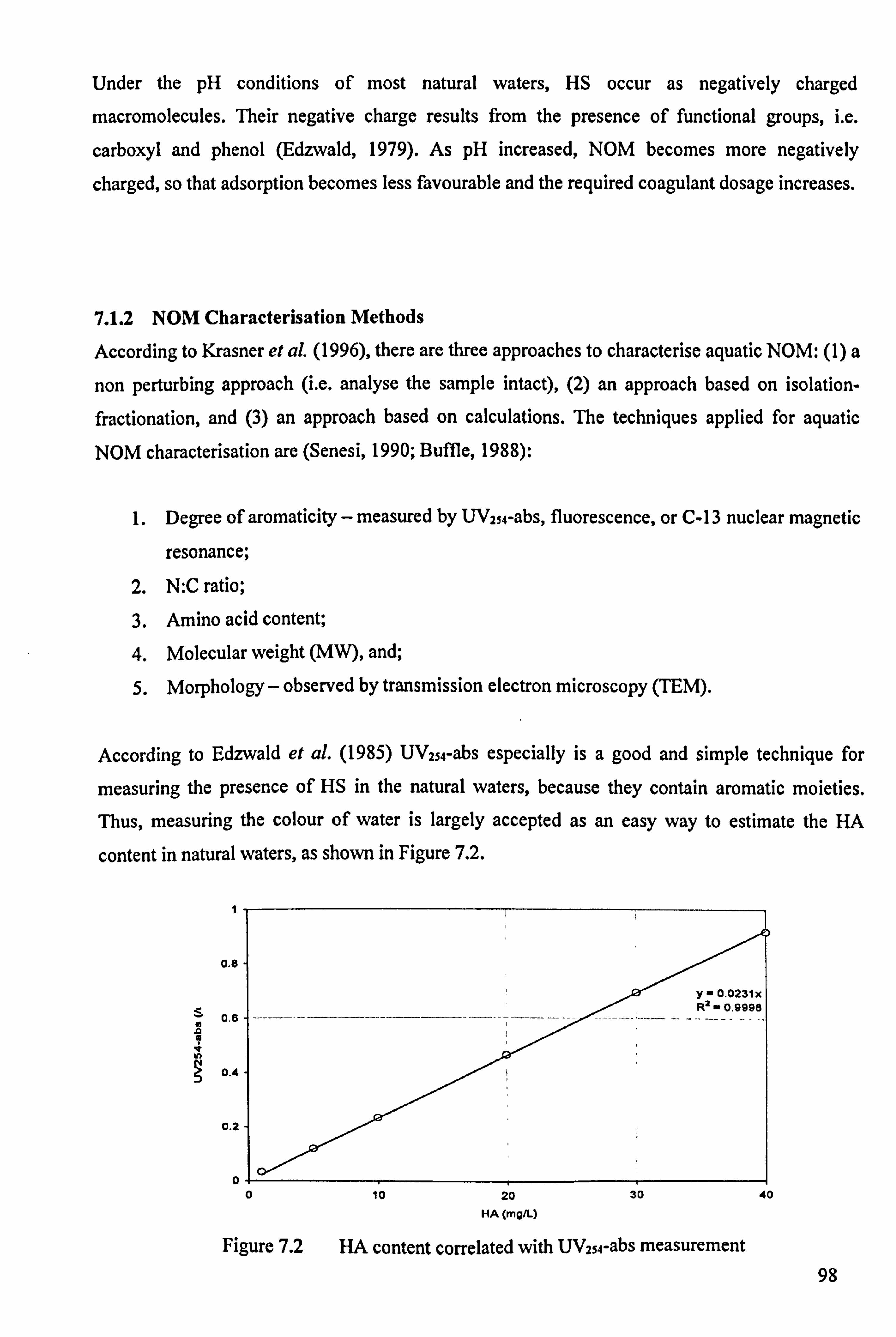
Under the pH conditions of most natural waters, HS occur as negatively charged
macromolecules. Their negative charge results from the presence of functional groups, i. e.
carboxyl and phenol (Edzwald, 1979). As pH increased, NOM becomes more negatively
charged, so that adsorption becomes less favourable and the required coagulant dosage increases.
7.1.2 NOM Characterisation Methods
According to Krasner et al. (1996), there are three approaches to characterise aquatic NOM: (1) a
non perturbing approach (i. e. analyse the sample intact), (2) an approach based on isolation-
fractionation, and (3) an approach based on calculations. The techniques applied for aquatic
NOM characterisation are (Senesi, 1990; Buffle, 1988):
1. Degree of aromaticity - measured by UV254-abs, fluorescence, or C-13 nuclear magnetic
resonance; 2. N: C ratio; 3. Amino acid content; 4. Molecular weight (MW), and;
5. Morphology - observed by transmission electron microscopy (TEM).
According to Edzwald et al. (1985) UV254-abs especially is a good and simple technique for
measuring the presence of HS in the natural waters, because they contain aromatic moieties. Thus, measuring the colour of water is largely accepted as an easy way to estimate the HA
content in natural waters, as shown in Figure 7.2.
1
0.8
0.6
0.4
0.2
0
y-0.0231x R2 0.9998
---------------
0 10 20 30 40
HA (mg/L)
Figure 7.2 HA content correlated with UV254-abs measurement 98

7.1.3 The Impacts of NOM on Water Treatment
The occurrence of NOM in raw drinking water can be problematic for water treatment because
of:
1. NOM's role in the transport and concentration of inorganic and organic pollutants (Randtke, 1988);
2. NOM's potential for serving as a substrates for biological growth in distribution systems (LeChevallier et al., 1991);
3. Increased chemical costs that result from increased coagulant and oxidant demands
(Crozes et al., 1995), and;
4. NOM's role as a precursor for potentially harmful DBPs (Merlet et al., 1992).
7.1.4 NOM Removal Technologies
The removal of NOM can be achieved by providing additional unit processes, such as adsorption
on activated carbon (GAC), membrane processes, chemical oxidation, or by enhancing the
existing coagulation, flocculation, and sedimentation processes (Jacangelo et. al., 1995).
Among these removal technologies, enhanced coagulation represents an economically attractive
option, as granular activated carbon (GAC) and membrane filtration and other alternative
technologies are comparatively much more expensive.
7.1.5 NOM Removal Mechanisms
As summarised by Randtke (1993), the major mechanisms by which NOM can be removed by
coagulation involved:
Colloidal destabilisation - can be caused by a compression of the double layer
surrounding the charger colloid, by charge neutralisation, by bridging, or by colloid
entrapment in the coagulant precipitate (sweep coagulation); Precipitation - NOM precipitation into a solid form as humates or fulvates because of lower solubility product formation, and; Co-precipitation - the soluble organic material is adsorbed onto the growing precipitate
of the metal hydroxide.
99

NOM Removal Mechanisms
Bridging Colloids removal Dissolved particles removal Specifically for organic polymers (influenced by
coagulant dose Colloid destabilisat ion Precipitation Co-precipitation
only) I
1. Double layer compression Sweep coagulation 2. Charge neutralisation
Lower pH Higher pH Lower coagulant dosages Higher coagulant dosages
Figure 7.3 Possible mechanisms for the removal of NOM by coagulation
Figure 7.3 shows the NOM removal mechanisms. The effects of higher coagulant dosage are
readily apparent, providing more metal for floc formation. Lower pH reduces the charge density
of humic acids, making them more hydrophobic and adsorbable, thus reducing the coagulant
dose.
Also, the coagulating species are more positively charged at lower pH. As a consequence,
adsorption becomes more favourable, and the coagulant dose decreases. The choice between
aluminium and iron simply reflects their different solubilities and coordination chemistry.
7.2 Model Water Preparation
Model coloured waters were prepared by humic acids (HA) and kaolin, to represent typical
lowland and upland waters in UK. Two colour solutions of varying HA concentrations plus turbidity were used for the colour removal tests.
Colour concentrations were obtained by using various amounts of humic acid' into tap water. Turbidity was obtained by adding a Kaolins. This silica clay had a particle size distribution of 0.1 to 4 µm. Turbidity levels in the model water solutions were in the range 2.76-8.86 NTU.
*Aldrich Chemical Co. tAldrich Chemical Co.
100
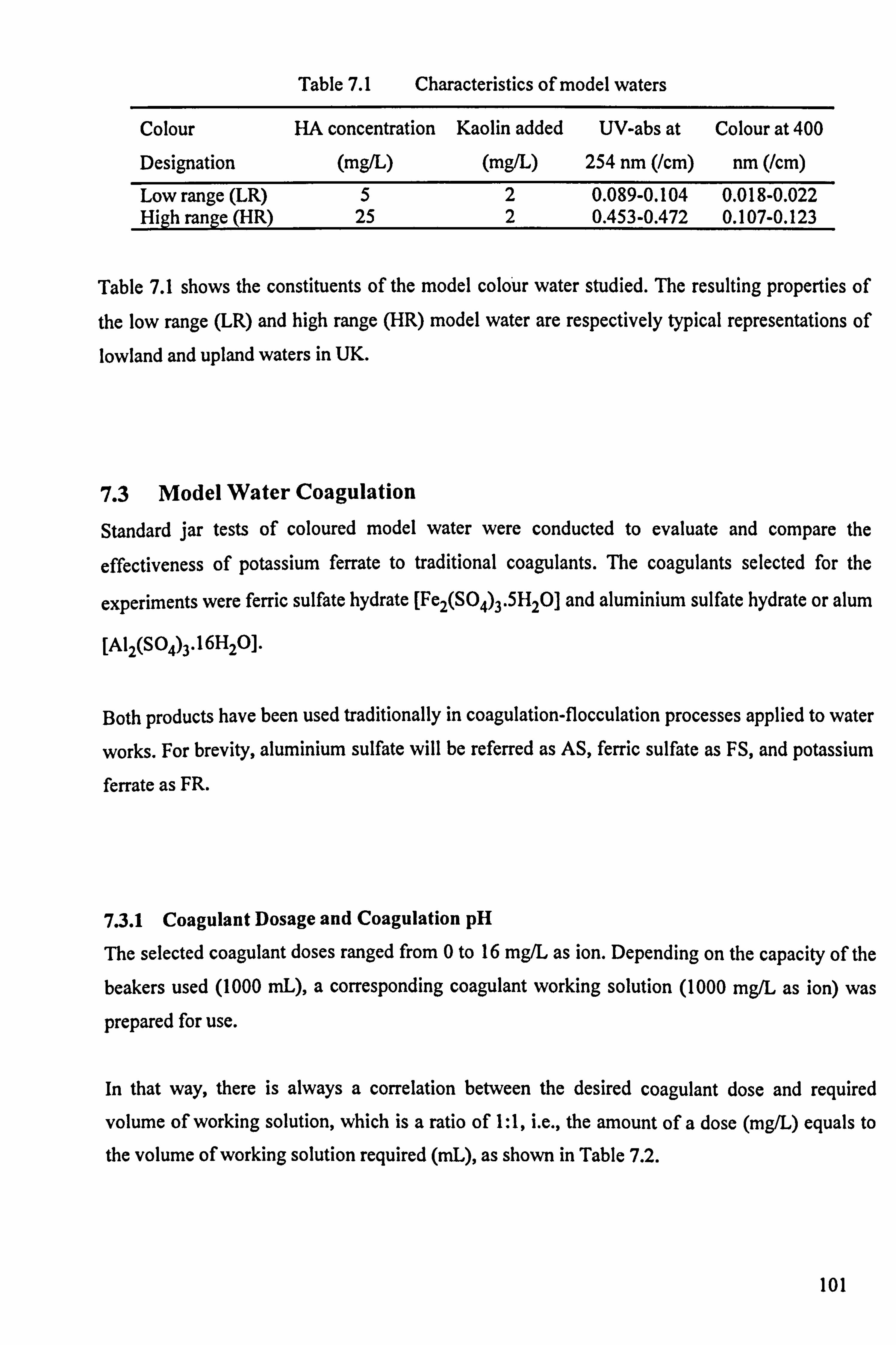
Table 7.1 Characteristics of model waters
Colour HA concentration Kaolin added UV-abs at Colour at 400
Designation (mg/L) (mg/L) 254 nm (/cm) nm (/cm)
Low range (LR) 520.089-0.104 0.018-0.022 High range (HR) 25 2 0.453-0.472 0.107-0.123
Table 7.1 shows the constituents of the model colour water studied. The resulting properties of
the low range (LR) and high range (HR) model water are respectively typical representations of lowland and upland waters in UK.
7.3 Model Water Coagulation
Standard jar tests of coloured model water were conducted to evaluate and compare the
effectiveness of potassium ferrate to traditional coagulants. The coagulants selected for the
experiments were ferric sulfate hydrate [Fe2(SO4)3.5H20] and aluminium sulfate hydrate or alum
[Al2(SO4)3.16H20].
Both products have been used traditionally in coagulation-flocculation processes applied to water
works. For brevity, aluminium sulfate will be referred as AS, ferric sulfate as FS, and potassium ferrate as FR.
7.3.1 Coagulant Dosage and Coagulation pH
The selected coagulant doses ranged from 0 to 16 mg/L as ion. Depending on the capacity of the beakers used (1000 mL), a corresponding coagulant working solution (1000 mg/L as ion) was
prepared for use.
In that way, there is always a correlation between the desired coagulant dose and required
volume of working solution, which is a ratio of 1: 1, i. e., the amount of a dose (mgfL) equals to
the volume of working solution required (mL), as shown in Table 7.2.
101
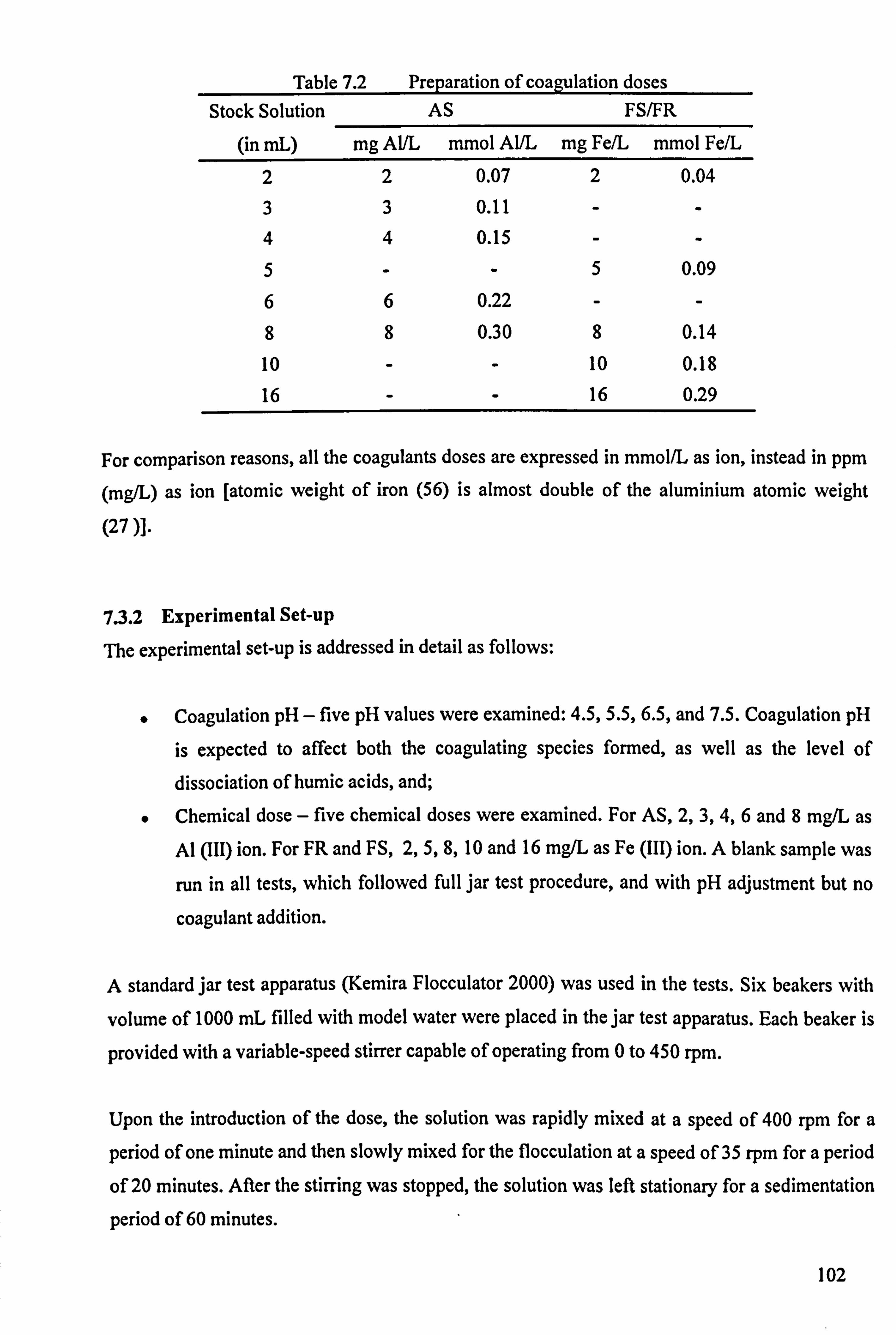
Table 7.2 Preparation of coagulation doses
Stock Solution AS FS/FR
(in mL) mg AVL mmol AWL mg Fe/L mmol Fe/L
220.07 2 0.04
330.11 -- 440.15 -- 5 --5 0.09
6 6 0.22 - - 8 8 0.30 8 0.14
10 -- 10 0.18
16 -- 16 0.29
For comparison reasons, all the coagulants doses are expressed in mmol/L as ion, instead in ppm
(mg/L) as ion [atomic weight of iron (56) is almost double of the aluminium atomic weight
(27 )].
7.3.2 Experimental Set-up
The experimental set-up is addressed in detail as follows:
Coagulation pH - five pH values were examined: 4.5,5.5,6.5, and 7.5. Coagulation pH
is expected to affect both the coagulating species formed, as well as the level of
dissociation of humic acids, and;
Chemical dose - five chemical doses were examined. For AS, 2,3,4,6 and 8 mg/L as Al (III) ion. For FR and FS, 2,5,8,10 and 16 mg/L as Fe (III) ion. A blank sample was
run in all tests, which followed full jar test procedure, and with pH adjustment but no
coagulant addition.
A standard jar test apparatus (Kemira Flocculator 2000) was used in the tests. Six beakers with
volume of 1000 mL filled with model water were placed in the jar test apparatus. Each beaker is
provided with a variable-speed stirrer capable of operating from 0 to 450 rpm.
Upon the introduction of the dose, the solution was rapidly mixed at a speed of 400 rpm for a
period of one minute and then slowly mixed for the flocculation at a speed of 35 rpm for a period
of 20 minutes. After the stirring was stopped, the solution was left stationary for a sedimentation
period of 60 minutes.
102

At the end of each experiment, the supernatant was taken and samples turbidity was firstly
measured. Subsequently, they were filtered through a 0.45 µm membrane before being analysed for the UV254-abs and colour at 400 nm.
In this Chapter, coagulation process is optimised for the removal of UV254-abs rather than
turbidity, as UV2sa-abs is a surrogate parameter to characterise NOM and HS (Edzwald et al.,
1985).
7.4 Model Water Coagulation Results
The principal indicators used for the evaluation of the effectiveness of the three coagulants in
enhancing the quality of coloured model water were residual turbidity and residual colour. These
residuals are calculated based on the measured values of the blanks (no coagulant addition, only
pH adjustment).
In the referring graphs for discussion, the numbers in the brackets indicate the values of the
parameters such as turbidity, UV254-abs, and colour (400 nm) of the blank samples (no coagulant
addition, only pH adjustment). The pH was adjusted by addition of sulphuric (H2S04) acid and
sodium hydroxide (NaOH).
7.4.1 Low Range Model Water
LR model waters are usually quite difficult to coagulate as they are rich in colour and at the same
time low in particle concentrations. At pH 4.5, turbidity removal of coagulants was maximum
above a coagulant dose of 0.07 mmol AWL and 0.04 mmol Fe/L, and did not significantly
deteriorate above these doses, except for FR, as shown in Figure 7.4.
However, turbidity removal of FR was maximum only below a coagulant dose of 0.09 mmol Fe/L, and deteriorated significantly above this dose, because of particle restabilisation by
overdosing.
In all the cases, the removal mechanism is believed to be associated with the charge
neutralisation and precipitation through Al/Fe hydrolysis species. The low pH of 4.5 reduces the
charge density of HA, making them more hydrophobic, and thus, adsorbable.
103
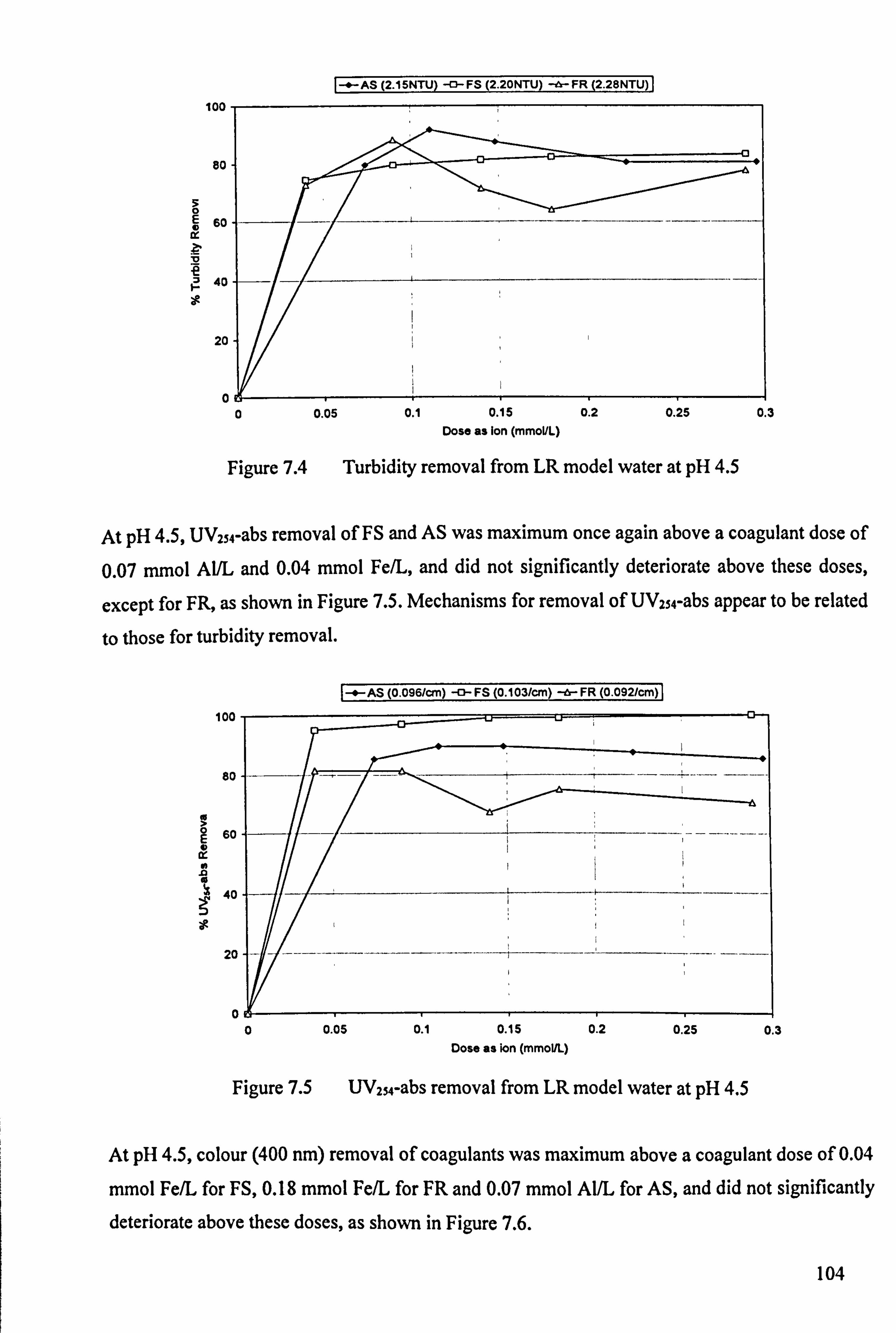
100 -*--AS (2.15NTU -0- FS (2.20NTU -a-FR 2.28NTU)
80
s 0 E 60
e v_
40
Z9
20
0 0 0.05 0.1 0.15 0.2 0.25 0.3
Dose as Ion (mmoVL)
Figure 7.4 Turbidity removal from LR model water at pH 4.5
At pH 4.5, UV254-abs removal of FS and AS was maximum once again above a coagulant dose of
0.07 mmol Al/L and 0.04 mmol Fe/L, and did not significantly deteriorate above these doses,
except for FR, as shown in Figure 7.5. Mechanisms for removal of UV254-abs appear to be related
to those for turbidity removal.
1-4--AS (0.096/cm) -a- FS (0.103/cm) -8- FR (0.092/cm)
100
80
60 0 a
ao
20
0 0.05 0.1 0.15 0.2 0.25 0.3 Dose as ion (mmolL)
Figure 7.5 UV2sa-abs removal from LR model water at pH 4.5
0
Li- 0-
i
i
- ----------- -- - ------- -- --- i
i
At pH 4.5, colour (400 nm) removal of coagulants was maximum above a coagulant dose of 0.04
mmol Fe/L for FS, 0.18 mmol Fe/L for FR and 0.07 mmol Al/L for AS, and did not significantly
deteriorate above these doses, as shown in Figure 7.6.
104

I-. -AS (0.018/cm) IFS (0.023/cm) -a-FR (0.019/cm)
100
80
E C C
0 60
E 40
0 ö U
20
06 1 0 0.05 0.1 0.15 0.2 0.25 0.3
Dose as ion (mmoIL)
Figure 7.6 Colour (400 run) removal from LR model water at pH 4.5
As the pH is increased at 5.5 and higher values, the coagulants dosages required for turbidity
were increased. This is because HA molecules become more stable as pH increases, a
phenomenon that results from the dissociation of functional groups, thus increasing the
magnitude of the negative charges.
Thus, at pH 5.5, turbidity removal of coagulants was maximum up to 0.15 mmol AWL and 0.14
mmol Fe/L, and significantly deteriorated above these doses, because of particle restabilisation
by overdosing, as shown in Figure 7.7.
ItAS (2.08NTU) -o- FS (1.89NTU) -e- FR (2.31 NTU
100
80
60
40
20
0 0.05 0.1 0.15 0.2 0.25 0.3 Dose as ion (mmolL)
Figure 7.7 Turbidity removal from LR model water at pH 5.5
0
....................
...
105

At pH 5.5, UV254-abs removal of coagulants was maximum above a coagulant dose of 0.11 mmol
Al/L and 0.09 mmol Fe/L, and did not significantly deteriorate above these doses, as shown in
Figure 7.8.
100
80 -
0 m 60 Q e a
40
20
0 0
Figure 7.8
0.05 0.1 0.15 0.2 0.25 0.3 Dose as Ion (mmol/L)
UV254-abs removal from LR model water at pH 5.5
Once more, the removal mechanism is believed to be associated with the charge neutralisation
and precipitation through At/Fe hydrolysis species. However, pH of 5.5 does not significantly
reduce the charge density of HA, making them less hydrophobic, and thus, less adsorbable.
At pH 5.5, colour (400 nm) removal of coagulants was maximum above a coagulant dose of 0.04
mmol Fe/L and 0.07 mmol AWL, and did not significantly deteriorate above these doses, as
shown in Figure 7.9.
I-'--AS (0.019/em -0- FS (0.021/cm -a- FR 0.020/cm
--*-AS (0.095/cm) -a- FS (0.098/cm) --a- FR 0.091 /cm
i
i
i
100
80
O O
60
40 0 ö U
20
0 0.05 0.1 0.15 0.2 0.25 0.3 Dose as Ion (mmoIL)
Figure 7.9 Colour (400 nm) removal from LR model water at pH 5.5
106
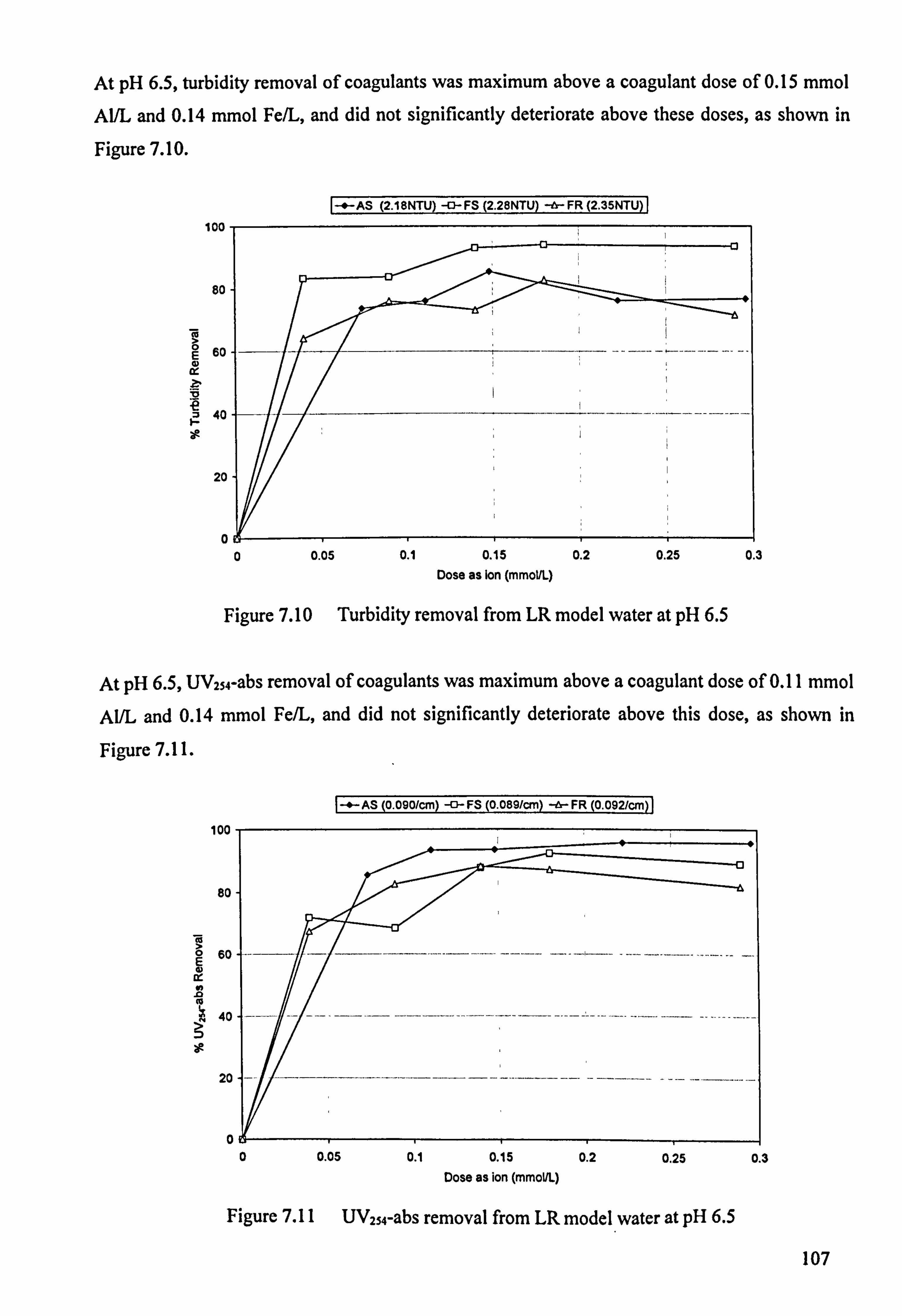
At pH 6.5, turbidity removal of coagulants was maximum above a coagulant dose of 0.15 mmol
Al/L and 0.14 mmol Fe/L, and did not significantly deteriorate above these doses, as shown in
Figure 7.10.
I--*-AS (2.18NTU -O-FS 2.28NTU -&-FR(2.35NTU
100
80
E 60 d
v F
40
20
0
0 0.05 0.1 0.15 0.2 0.25 0.3 Dose as on (mmol/L)
Figure 7.10 Turbidity removal from LR model water at pH 6.5
At pH 6.5, W254-abs removal of coagulants was maximum above a coagulant dose of 0.11 mmol
Al/L and 0.14 mmol Fe/L, and did not significantly deteriorate above this dose, as shown in
Figure 7.11.
100
80
1-4-AS (0.0901cm) -a--FS 0.089/cm -0- FR 0.092/Cm
E 60 N ir h
l0
40
20
0 0.05 0.1 0.15 0.2 0.25 0.3 Dose as ion (mmoll)
Figure 7.11 UV254-abs removal from LR model water at pH 6.5
107

At pH 6.5, colour (400 nm) removal of coagulants was maximum above a coagulant dose of 0.04
mmol Fe/L for FS, 0.14 mmol Fe/L for FR and 0.07 mmol AWL for AS, and did not significantly
deteriorate above these doses, as shown in Figure 7.12.
I -. --AS 0.021/cm -0- FS 0.022/cm --a- FR 0.019/cm
100
80
ii i
ý'I
'. ý, i iýi
-t-------r-----. _ýý _.. ý
'
_. l. ___. ______ýI-
'ýI
E C 0 ° 60
0 E m
40 5 0 ö U
29 20
0 0 0.05 0.1 0.15 0.2 0.25 0.3
Dose as Ion (mmol/L)
Figure 7.12 Colour (400 nm) removal from LR model water at pH 6.5
At pH 7.5, turbidity removal of AS and FS was maximum above a coagulant dose of 0.07 mmol
Al/L and 0.14 mmol Fe/L, and did not significantly deteriorate above these doses, as shown in
Figure 7.13. However, FR did not perform well, as part of ferrate remained stable at high pH,
resulting in colouring of the treated samples.
I tAS (2.11NTU) -o- FS (2.1ONTU) --b- (FR (2.27NTU)
100
80
0 E 60
40 e
20
0 0.05 0.1 0.15 0.2 0.25 0.3 Dose as Ion (mmol/L)
Figure 7.13 Turbidity removal from LR model water at pH 7.5
0
108

At pH 7.5, UV254-abs removal of coagulants was maximum above a coagulant dose of 0.15 mmol
AWL and 0.04 mmol Fe/L, and did not significantly deteriorate above these doses, as shown in
Figure 7.14.
100
80
E 60 E tr n a is
40
20
0
I -. -AS (0.09 1/cm -o- FS 0.104/cm -b-FR 0.091 /cm
i
i
--- -- - --- ----
0 0.05 0.1 0.15 0.2 0.25 0.3 Dose as Ion (mmolL)
Figure 7.14 UV254-abs removal from LR model water at pH 7.5
At pH 7.5, colour (400 nm) removal of coagulants was maximum above a coagulant dose of 0.04
mmol Fe/L and 0.07 mmol AWL, and did not significantly deteriorate above these doses, as
shown in Figure 7.15.
100
80
E C C
60
0 E d
40 0 0 U
20
0
I tAS (0.022/cm -0-FS (0.020/cm) -A- FR 0.021/cm
0 0.05 0.1 0.15 0.2 0.25 0.3 Dose as ion (mmolL)
Figure 7.15 Colour (400 nm) removal from LR model water at pH 7.5
109

At pH values above 6.5, precipitation of metal hydroxides [AI(OH)3(, ) and Fe(OH)3(, )]occurs,
shifting the removal mechanism from precipitation to co-precipitation. As pH increases, HA
becomes more negatively charged and the coagulating species become less positively charged, so
that adsorption becomes less favourable and the required dosage increases.
7.3.2 High Range Model Water
High range (HR) model waters are usually quite difficult to coagulate as they are very rich in
colour and at the same time low in colloidal particles. At pH 4.5, turbidity removal of coagulants
was maximum above a coagulant dose of 0.11 mmol Al/L and 0.09 mmol Fe/L, and did not
significantly deteriorate above these doses, as shown in Figure 7.16.
The removal mechanism is believed to be associated with the charge neutralisation and
precipitation through Al/Fe hydrolysis species, because the low pH of 4.5 reduces the charge
density of HA, making them more hydrophobic, and thus, adsorbable.
-0 -AS 7.30NTU IFS . 20NTU -A--FR 7.18NTU
100
80
E 60 d
Z, V 40
20-
0 0.00 0.05 0.10 0.15 0.20 0.25 0.30
Dose as ion (mmol/L)
Figure 7.16 Turbidity removal from HR model water at pH 4.5
At pH 4.5, UV254-abs removal of coagulants was maximum once again above a coagulant dose of
0.11 mmol Al/L and 0.09 mmol Fe/L, and did not significantly deteriorate above these doses, as
shown in Figure 7.17. Mechanisms for removal of UV254-abs appear to be related to those for
turbidity removal.
110

100
80
9
0 60
4o
20
0
I--*-AS (0.461 /CM) -Ch- FS (0.468/cm) -, - FR (0.453/cm)
i
I
__
0.00 0.05 0.10 0.15 0.20 0.25 0.30 Dose as Ion (mmol/L)
Figure 7.17 UV254-abs removal from HR model water at pH 4.5
At pH 4.5, colour (400 nm) removal of coagulants was maximum above a coagulant dose of 0.04
mmol Fe/L and 0.07 mmol AVL, and did not significantly deteriorate above these doses, as
shown in Figure 7.18.
100
80
E C C G
60
0 E 0
40 ö U
20
0 Is i 0.00 0.05 0.10 0.15 0.20 0.25 0.30
Dose as ion (mmoIL)
Figure 7.18 Colour (400 nm) removal from HR model water at pH 4.5
As the pH is increased at 5.5 and higher values, the coagulants dosages required for turbidity
were increased. This is because HA molecules become more stable as pH increases, a
phenomenon that results from the dissociation of functional groups, thus increasing the
magnitude of the negative charges.
111
1-*-AS (0.107/cm) -o- FS (0.118/cm) -&-FR (0.121/cm)

Therefore, at pH 5.5, turbidity removal of coagulants was maximum above a coagulant dose of
0.22 mmol AWL and 0.18 mmol Fe/L, and did not significantly deteriorated above these doses, as
shown in Figure 7.19.
100
80
I-*-AS . 08NTU -o- FS (7.28NTU) -8- FR 7.27NTU)
A
0 60 0 Ix 41
40
29
20
o 0.00 0.05 0.10 0.15 0.20 0.25 0.30
Dose as ion (mmolJL)
Figure 7.19 Turbidity removal from HR model water at pH 5.5
At pH 5.5, UV254-abs removal of coagulants was maximum above a coagulant dose of 0.07 mmol
Al/L and 0.09 mmol Fe/L, and did not significantly deteriorate above these doses, as shown in
Figure 7.20.
100
80
60
40
20
-+-AS(0.454/cm -C>- FS (0.465/cm -a- FR 0.461/cm
0.00 0.05 0.10 0.15 0.20 0.25 0.30 Dose as on (mmoUL)
Figure 7.20 WZSe-abs removal from HR model water at pH 5.5
0
112
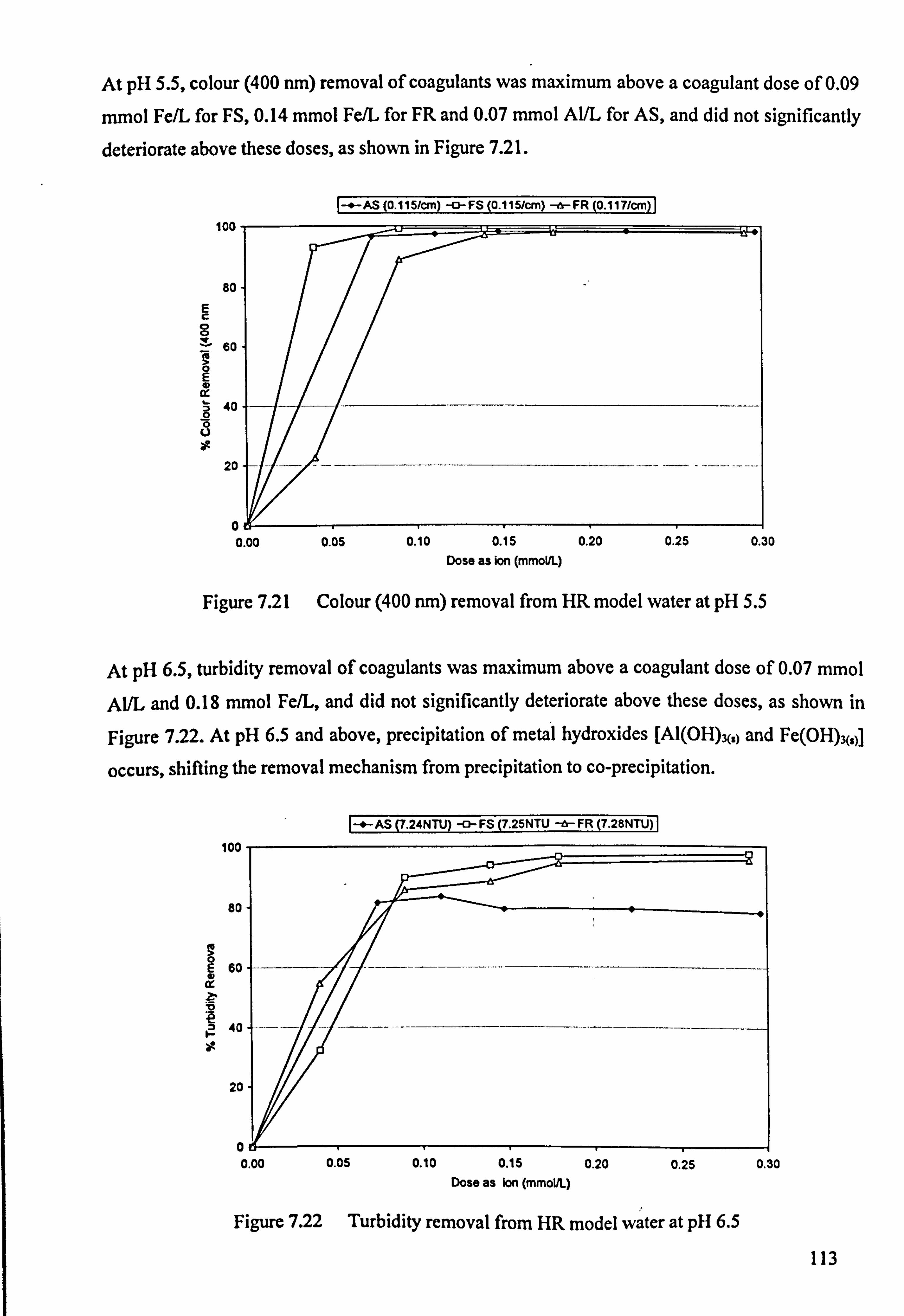
At pH 5.5, colour (400 nm) removal of coagulants was maximum above a coagulant dose of 0.09
mmol Fe/L for FS, 0.14 mmol Fe/L for FR and 0.07 mmol AWL for AS, and did not significantly
deteriorate above these doses, as shown in Figure 7.21.
100
80
I-. --AS (0.115/Cm -o- FS (0.115/cm) -a- FR (0.1 117/cm
E c 0
60
0 E 0 ix
40 0
20
06 1 0.00 0.05 0.10 0.15 0.20 0.25 0.30
Dose as ion (mmolL)
Figure 7.21 Colour (400 nm) removal from HR model water at pH 5.5
At pH 6.5, turbidity removal of coagulants was maximum above a coagulant dose of 0.07 mmol
Ai/L and 0.18 mmol Fe/L, and did not significantly deteriorate above these doses, as shown in
Figure 7.22. At pH 6.5 and above, precipitation of metal hydroxides [Al(OH)3(1) and Fe(OH)3(, )}
occurs, shifting the removal mechanism from precipitation to co-precipitation.
100
80
1-4-- AS (7.24NTU) -a--FS (7.25NTU --BFR 7.28NTU)
0 E 60
e
40
9
20
0.00 0.05 0.10 0.15 0.20 0.25 Dose as Ion (mmoUL)
Figure 7.22 Turbidity removal from HR model water at pH 6.5
113

At pH 6.5, UV2s. -abs removal of coagulants was maximum above a coagulant dose of 0.07 mmol
Al/L and 0.09 mmol Fe/L, and did not significantly deteriorate above these doses, as shown in
Figure 7.23.
100
80
-*. -AS (0.477/cm -0- FS (0.469/cm) -e- FR (0.462/Cm)
N
0 E 60
d
40
20
0 is iII -i 0.00 0.05 0.10 0.15 0.20 0.25 0.30
Dose as ion (mmolL)
Figure 7.23 UV254-abs removal from HR model water at pH 6.5
At pH 6.5, colour (400 run) removal of coagulants was maximum above a coagulant dose of 0.09
mmol Fe/L and 0.07 mmol AWL, and did not significantly deteriorate above these doses, as
shown in Figure 7.24.
100
80
E
0 0 60
0 E 0 § 40
ci
20
I-. - AS 0.118/cm -0- FS 0.117/cm -8- FR 0.120/cm
0.00 0
Dose as ion (mmoUL)
Figure 7.24 Colour (400 run) removal from HR model water at pH 6.5
114

At pH 7.5, turbidity removal of coagulants was maximum above a coagulant dose of 0.11 mmol Al/L and 0.18 mmol Fe/L, and did not significantly deteriorate above these doses, as shown in
Figure 7.25.
100
80
4
-. -AS . 21NTU -0-FS . 30NTU -a-FR 7.22NTU
E 60
v_
40
20
0 0.00 0.05 0.10 0.15 0.20 0.25 0.30
Dose as ion (mmoUL)
Figure 7.25 Turbidity removal from HR model water at pH 7.5
At pH 7.5, UV254-abs removal of coagulants was maximum above a coagulant dose of 0.11 mmol
AWL and 0.09 mmol Fe/L, and did not significantly deteriorate above these doses, as shown in
Figure 7.26. However, FR did not perform well, as part of ferrate remained stable at high pH,
resulting in colouring of the treated samples.
-*-AS (0.477/cm) -o- FS (0.475/cm) -&-FR 0.466/Cm
100
80
A 0 60
N a 3
g40
20
0.00 0.05 0.10 0.15 0.20 0.25 0.30 Dose as ion (mmoVL)
Figure 7.26 UV254-abs removal from HR model water at pH 7.5
0
115

At pH 7.5, colour (400 nm) removal of coagulants was maximum above a coagulant dose of 0.09
mmol Fe/L and 0.07 mmol AUL, and did not significantly deteriorate above these doses, as
shown in Figure 7.27.
100
80
E c 0 0
60 m 0 E 0
ö 40
0 U
ag 20
0
-*-AS (0.123/cm) -o- FS (0.119/cm) -a- FR (0.120/Cm
i
i
i
i
1
i
0.00 0.05 0.10 0.15 0.20 0.25 0.30 Dose as ion (mmol/L)
Figure 7.27 Colour (400 run) removal from HR model water at pH 7.5
7.5 Discussion
The use of FR for coagulation/flocculation of coloured model water gave promising results for its
possible future use in the water industry, although FS performed better than FR and AS. Two
kinds of model water were prepared in the laboratory, both rich in colour and low in colloids.
Natural waters that have these specific characteristics are usually low rivers and upland
catchments. Coagulants performance for both model waters is summarised in Tables 7.3 and 7.4.
Table 7.3 Turbidity, UV254-abs, and colour removal of coagulants
LR model water HR model water Turbidity UV2s, -abs Colour (400 nm) Turbidity W254-abs Colour (400 nm)
(%) (%) % (%) (%) %
AS 61-92 78-98 94-100 75-96 84-99 96-99 FS 63-94 72-100 97-100 26-98 79-100 90-100 FR 61-88 67-91 84-100 5-95 79-99 23-98
116
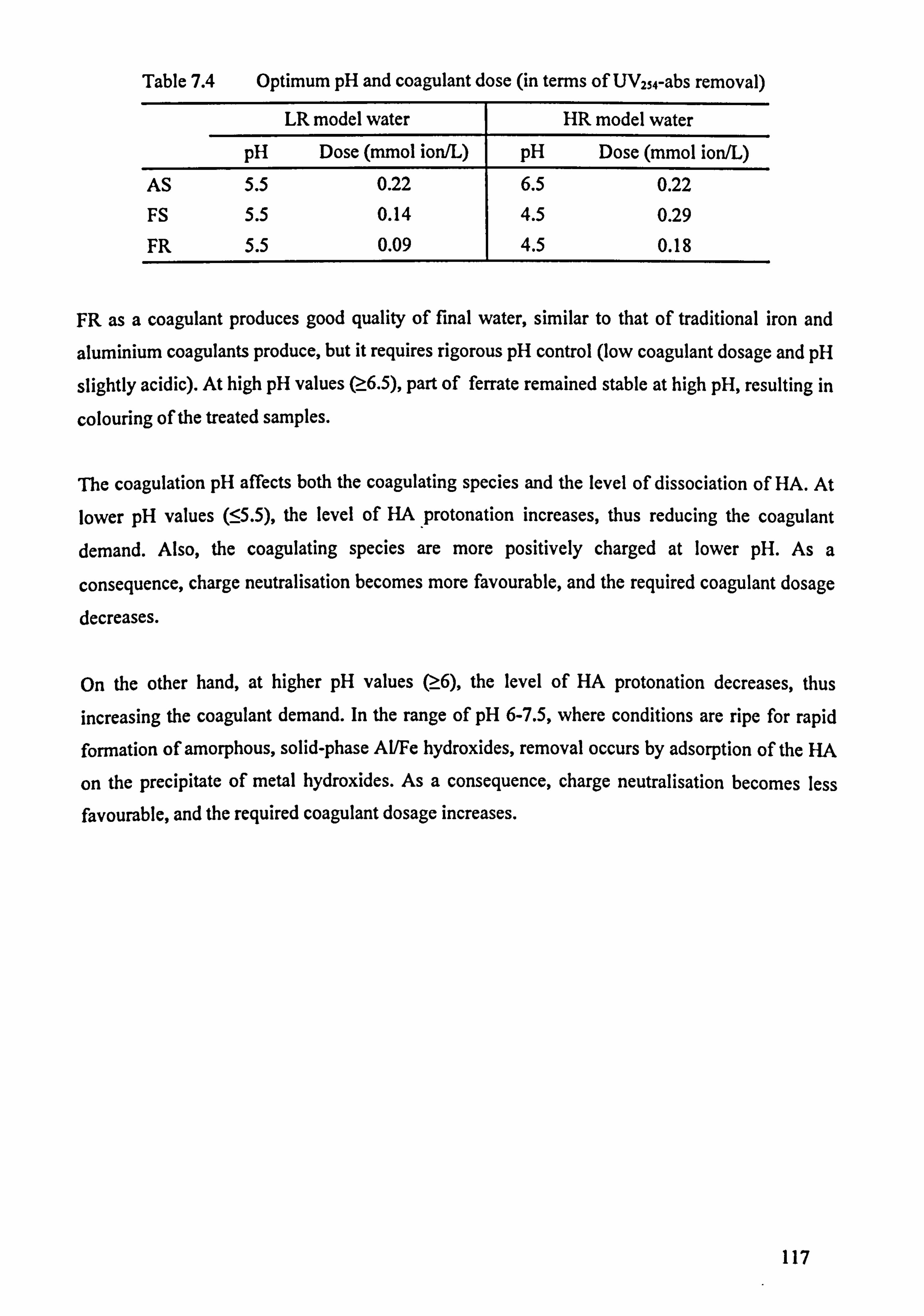
Table 7.4 Optimum pH and coagulant dose (in terms of UV254-abs removal)
LR model water HR model water
pH Dose (mmol ion/L) pH Dose (mmol ion/L)
AS 5.5 0.22 6.5 0.22 FS 5.5 0.14 4.5 0.29 FR 5.5 0.09 4.5 0.18
FR as a coagulant produces good quality of final water, similar to that of traditional iron and
aluminium coagulants produce, but it requires rigorous pH control (low coagulant dosage and pH
slightly acidic). At high pH values (? 6.5), part of ferrate remained stable at high pH, resulting in
colouring of the treated samples.
The coagulation pH affects both the coagulating species and the level of dissociation of HA. At
lower pH values (55.5), the level of HA protonation increases, thus reducing the coagulant
demand. Also, the coagulating species are more positively charged at lower pH. As a
consequence, charge neutralisation becomes more favourable, and the required coagulant dosage
decreases.
On the other hand, at higher pH values (? 6), the level of HA protonation decreases, thus
increasing the coagulant demand. In the range of pH 6-7.5, where conditions are ripe for rapid formation of amorphous, solid-phase Al/Fe hydroxides, removal occurs by adsorption of the HA
on the precipitate of metal hydroxides. As a consequence, charge neutralisation becomes less
favourable, and the required coagulant dosage increases.
117

Untreated waters usually contain finely divided matter, which must he removed before
distribution for domestic and industrial use. Safety and aesthetics dictate that all potable water
should be free of suspended matter. Coagulant use is necessary to achieve charge neutralisation
and facilitate particle aggregation, necessary for the sedimentation and filtration process to work
properly.
In the first part of this Chapter, the river water characteristics and experimental set-up are briefly
outlined. In the second part of this Chapter, the coagulation and disinfection results of the treated
river water are presented and discussed.
8.1 River Water
River water samples were collected from the inlet (prior to screening) of a water treatment plant
of Thames Water in Shalford, Surrey. Samples were collected using high density polyethylene
(HDPE) jerricans, which were washed and rinsed with tap water before use. "There is a variation
in the values of the parameters as a result of weather conditions depending on the season
(dry/wet), as shown in Table 8.1.
Table 8.1 Characteristics of river water during June-August 2002
Parameter Range Mean Value
pH 7.65-7.86 7.76
Turbidity (NTU) 2.14-14.77 8.46
Total Suspended Solids (mg/100 mL) 0.055-0.078 0.067
UV-abs at 254 nm (cm"') 0.042-0.075 0.059
Colour as Vis-abs at 400 nm (cm-') 0.005-0.011 0.008
Total Coliform (per 100 mL) 4-20x104 12x10^
Faecal Coliform (per 100 mL) 9-25x10' 17x 10'
118

8.2 River Water Coagulation
Standard jar tests were conducted to evaluate and compare the coagulation and disinfection
effectiveness of potassium ferrate (FR) to traditional coagulants such as ferric sulfate (FS) and
aluminium sulfate (AS).
8.2.1 Coagulant Dosage
As detailed in Chapter 7, the selected coagulant doses ranged from 0 to 16 mg/L as ion.
Depending on the sample volume (1000 mL), a corresponding stock coagulant solution (1000
mg/L as ion) was prepared for use. In that way, there is a positive correlation between desired
coagulant dose and required volume of stock solution to achieve it and this is one to one (1: 1), as
shown in Table 8.2.
Table 8.2 Preparation of coagulation doses
Stock Solution
(in mL) mg Al/L
AS
mmol AWL
FS/FR
mg Fe/L mmol Fe/L
2 2 0.07 2 0.04 3 3 0.11 -- 4 4 0.15 -- 5 - - 5 0.09 6 6 0.22 -- 8 8 0.30 8 0.14 10 - - 10 0.18 16 - - 16 0.29
Once more as in Chapters 6 and 7, for comparing the performance based on the equivalent
coagulant doses, all coagulants doses are expressed in mmol/L as ion, instead in ppm (mg/L) as ion.
8.2.2 Experimental Set-up
There may be many factors that could influence the performance of any given coagulant, such as characteristics of the treated water, coagulation pH, chemical dosage, and jar test set-up. However, in this set of experiments only chemical dosage and coagulation pH are of interest. The
experimental set-up is addressed in detail as follows:
119
Coagulation pH - five pH values were examined: 4,5,6,7, and 8. Coagulation pH is
expected to affect both the coagulating species formed, as well as the level of bacteria
inactivation, and;
Chemical dose - five chemical doses were examined. For AS, 2,3,4,6 and 8 mg AI/L.
For FR and FS, 2,5,8,10 and 16 mg Fe/L.
In each jar test run, there was a blank sample, where no coagulant was added but only pH
adjustment was carried out and the sample followed whole jar test procedures. A standard jar test
apparatus (Kemira Flocculator 2000) was used in the tests. Six beakers with volume of 1000 mL filled with raw water were placed in the jar test apparatus.
Upon the introduction of the dose, the solutions were rapidly mixed at a speed of 400 rpm for a
period of one minute and then allowed to flocculate at a speed of 35 rpm for a period of 20
minutes. After the stirring is stopped, samples were allowed to settle for a period of 60 minutes.
At the end of each experiment, supernatants were withdrawn and water quality parameters were
measured, including turbidity, UV254-abs, colour (vis-abs at 400 nm), and bacteria (total coliform
and faecal coliform). Measurement of turbidity, UV254-abs and colour followed the Standard
Methods (APHA, 1998), and the samples need filtered by a 0.45 mm membrane before
measuring UV254-abs and colour. Total and faecal coliform are measured before and after disinfection by membrane filtration method as described in Section 5.3.2.3.
8.3 Comparative Coagulation/Disinfection Performance
The principal indicators used for the evaluation of the effectiveness of the three coagulants in
treating river water were residual turbidity, residual UV254-abs, colour (400 nm), and inactivated
bacteria. The residuals are calculated based on the measured values of the blank samples (no
coagulant addition, only pH adjustment). The pH was adjusted by addition of sulphuric acid (H2S04) and sodium hydroxide (NaOH).
The abbreviations AS, FS and FR appeared in the graphs, stand respectively for aluminium
sulfate, ferric sulfate and potassium ferrate. The numbers in the brackets indicate the values of
quality parameters of blank samples such as turbidity, UV254-abs, colour (Vis-abs at 400 nm),
and faecal and total coliforms.
120

As shown in Figure 8.1, at pH 4, turbidity removal with iron based coagulants was maximum
when a coagulant dose was greater than 0.018 mmol Fe/L, and did not significantly deteriorate.
The performance of AS improved as dosage increased when doses were >0.018 mmol Fe/L. The
removal mechanism is believed to be associated with the charge neutralisation and precipitation
through Al/Fe hydrolysis species.
I tAS (7.59NTU) -0- FS (3.59NTU) -d- FR (4.11NTU)
100
80 -
E 60
" v
H 40
iI II
0 0.00 0.05 0.10 0.15 0.20 0.25 0.30
Dose (mmoVL)
Figure 8.1 Turbidity removal from river water at pH 4
In terms of UV254-abs removal, the coagulants did not achieve removal rates greater than 80 per
cent even at their highest dose, as shown in Figure 8.2. The performance of FR was by far better
than its rivals, mainly because of its high redox potential.
-+ AS (0.065/cm) -0- FS (0.048/cm) -e-FR 0.054/cm
100
80
0 E 60
E c a N
40
20
0.00 0.05 0.10 0.15 0.20 0.25 0.30
Dose (mmol/L)
Figure 8.2 UV254-abs removal from river water at pH 4
0
I I ýII
i
I
777 -- - -- - ---------1-- --''
IIIi
i Ij
I
121

As shown in Figure 8.3, at pH 4, colour removal (400 nm) of iron based coagulants was
maximum when a coagulant dose was either 0.08 mmol Fe/L for FR, or 0.14 mmol Fe/L for FS,
and did not significantly deteriorate when doses were greater than the performance of AS that
improved as dosage increased.
+- AS 0.005/cm -0- FS 0.004/cm --&- FR 0.005/cm
100
80 I
i
. _. .. _,.., _.... __. L.. _ _ _....... ... .... _. i
___ j
__-_ _ _.. __. _.. ___. _ a..
_ . ... _..... _. Y,. .....
i
_-i-_- T_____. _. __. ____. ____. ___. __ .. __ _.. _.. _. _ . i_
_ ..
i
60
40
8 it
20
0 0.00 0.05 0.10 0.15 0.20 0.25 0.30
Dose (mmoIL)
Figure 8.3 Colour (400nm) removal from river water at pH 4
At pH<5, all coagulants achieved completely inactivation, mainly due to the low pH value, rather than the coagulation process.
As shown in Figure 8.4, at pH 5, the iron based coagulants performed similar to before over
whole dose range studied, while the performance of AS was improved at lower doses compared to that at pH 4.
100
80
0 E 80
v_
f' 40 ä
20
0
-. -AS (7.49NTU) -D-FS 3.87NTU -e- FR 4.15NTU
0.00 0.05 0.10 0.15 0.20 0.25 0.30
Dose (mmoVL)
Figure 8.4 Turbidity removal from river water at pH 5 122
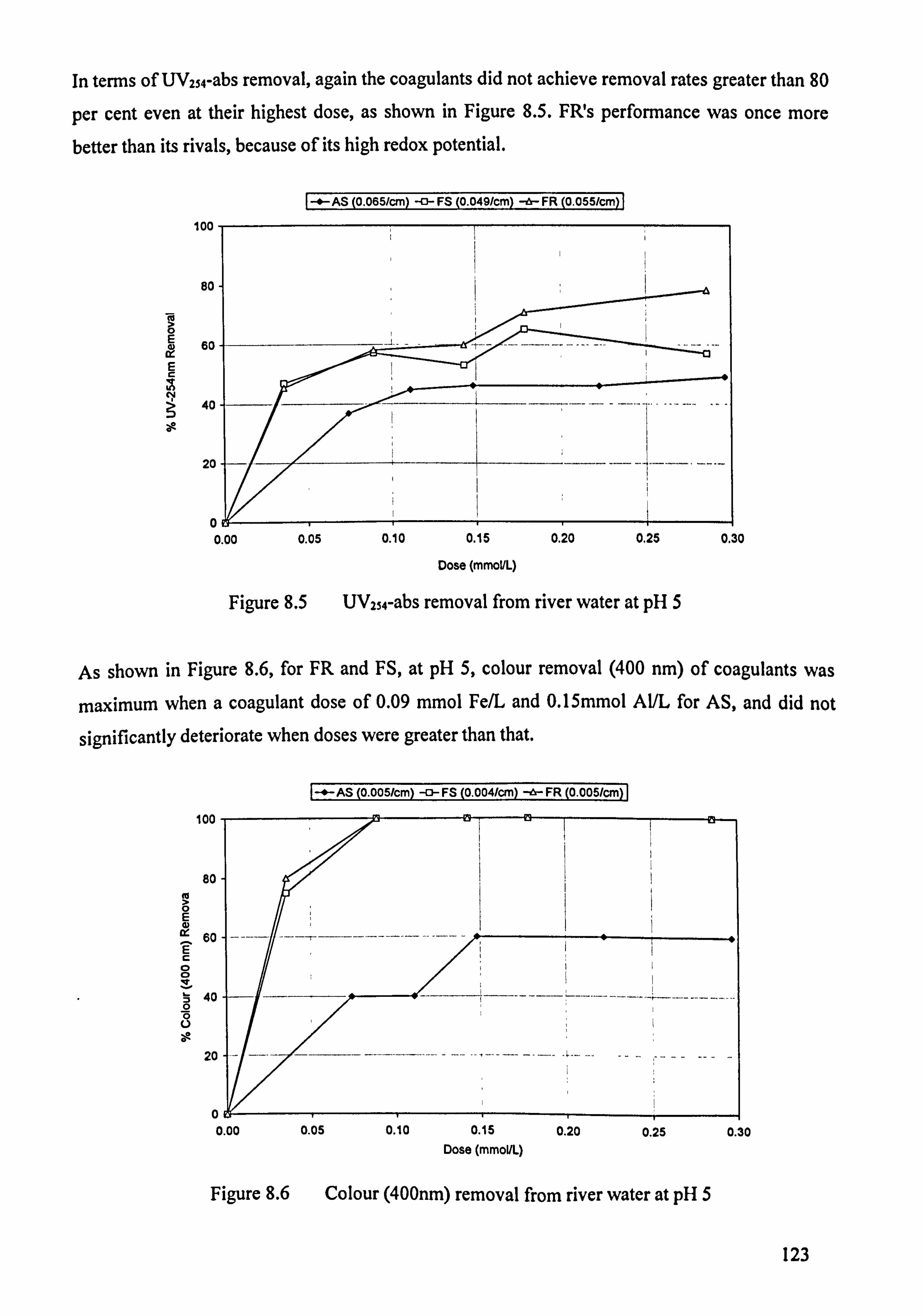
In terms of UV254-abs removal, again the coagulants did not achieve removal rates greater than 80
per cent even at their highest dose, as shown in Figure 8.5. FR's performance was once more
better than its rivals, because of its high redox potential.
I-+-AS (0.065/cm) -0- FS 0.049/cm -&- FR 0.055/cm
100
80
& 60
c
40
20
0
i
i
il
ii
0.00 Dose (mmowL)
Figure 8.5 UV254-abs removal from river water at pH 5
As shown in Figure 8.6, for FR and FS, at pH 5, colour removal (400 nm) of coagulants was
maximum when a coagulant dose of 0.09 mmol Fe/L and 0.15mmol Al/L for AS, and did not
significantly deteriorate when doses were greater than that.
-. -AS (0.005/cm) -G-FS 0.004/cm -e- FR 0.005/cm
100 710 29 ; 13 11 -'--1
80
0 E d
60 E c 0 0
40 0 0 U
20
0
ýý ýý
ýj ýI -ý ii
i
0.00 0.05 0.10 0.15 0.20 0.25 0.30 Dose (mmol/L)
Figure 8.6 Colour (400nm) removal from river water at pH 5
123

At pH 6, turbidity removal with AS was improved significantly, as shown in Figure 8.7. This is
owing to the predominance of Al hydroxide over other Al complex ions produced during
coagulation. However, the turbidity removal with iron based coagulants was not as good as that
with AS for the doses lower than 0.14 mmol/L as ion.
AS (10.8NTU) -0- FS (6.27NTU) -a- FR (5.8NTU)
100
80
60
2
40
20
0 0.00 0.05 0.10 0.15 0.20 0.25 0.30
Dose (mmol/L)
Figure 8.7 Turbidity removal from river water at pH 6
In terms of UV254-abs removal, FR achieved again an overall better performance, as shown in
Figure 8.8. However, comparing to pHs 4 and 5, the UV254-abs removal with traditional
coagulants was improved, as pH 6 permits the formation of more Al and Fe hydroxides, rather than other metal complex ions.
-*-AS (0.068/cm) -D- FS (0.058/cm) -A- FR 0.047/cm
100
80
60
E c a N N
40
20
0
it f
i
i
i
i
i
`_ i
ýý
0.00 0.05 0.10 0.15 0.20 0.25 0.30
Dose (mmolL)
Figure 8.8 UV254-abs removal from river water at pH 6
124

At pH 6, colour (400 nm) removal with AS was improved significantly, as shown in Figure 8.9.
However, the colour removal with iron based coagulants was still better than AS for doses as low
as 0.04 mmol Fe/L for FR, and 0.09 mmol Fe/L for FS.
-. -AS(0.007/cm)-e- FS (0.004/cm) -A- FR (0.001/cm)
100 ý0 0- 13 " a:,
80 i
.. _....
E w
60 E c 0 0
40 0 ö U el
20
0 0.00 0.05 0.10 0.15 0.20 0.25 0.30
Dose (mmol/L)
Figure 8.9 Colour (400nm) removal from river water at pH 6
At pH 6, FR achieved completely inactivation rates for the whole dose range studied, due to its
high redox potential, as shown in Figure 8.10. The inactivation performance of traditional
coagulants was similar to their turbidity performance, as more flocs are formed, more bacteria is
likely to be removed by flocs entrapment.
--*-AS (150000) -o- FS (43500) -0- FR 52000
100
80
S
60 O
3 0 V 40
0
20
0.00 0.05 0.10 0.15 0.20 0.25 0.30
Dose (mmol/L)
Figure 8.10 Bacteria inactivation from river water at pH 6
0
i
1
125

At pH 7, all coagulants have similar performance in terms of turbidity removal for doses greater
than 0.18 mmol/L as ion, as shown in Figure 8.11. However, the performance of FR started to
deteriorate for doses lower than 0.18 mmol/L as ion, mainly due to poor floc formation. This
results in flocs that are not heavy enough to precipitate out during the settling time of 60 minutes.
It AS (5.46NTU) FS (5.57NTU) -a- FR (5.16NTU) j
100
80 ---
E 60
40
20
0 0.00 0.05 0.10 0.15 0.20 0.25 0.30
Dose (mmovL)
Figure 8.11 Turbidity removal from river water at pH 7
In terms of UV254-abs removal, FR had an overall better performance than its rivals due to its
high redox potential, as shown in Figure 8.12. In general, UV2s4-abs removal with iron based
coagulants was still better than AS over whole dose range studied.
1-0--AS (0.066/Cm) -o- FS (0.044/cm) -a-FR (0.042/cm
100
80
I 0 0 60 It E c x N
40
29
20
0
---
0.00 0.05 0.10 0.15 0.20 0.25 0.30
Dose (mmolL)
Figure 8.12 UV254-abs removal from river water at pH 7
126

At pH 7, colour (400 nm) removal with AS was reduced compared to that at pH 6. Once more, the colour removal with iron based coagulants was better than AS over whole dose range studied,
as shown in Figure 8.13.
100
80
I-SAS (0.006/cm) -e-FS (0.002/cm) -A-FR (0.001/cm) I
Ii .. i
iI i K
(
e 0 E a,
60 E c 0 0 v ti 40 0 0 U
20
0 0.00 0.05 0.10 0.15 0.20 0.25 0.30
Dose (mmoVL)
Figure 8.13 Colour (400nm) removal from river water at pH 7
Same as at pH 6, FR achieved completely inactivation for the whole dose range studied, as
shown in Figure 8.14. Once more, the inactivation performance of traditional coagulants was
similar to their turbidity performance, as more flocs are formed, more bacteria is likely to be
removed by flocs entrapment.
It AS (135000) -0- FS (90000) -6- FR (195000)1
100
80
0
>
60
V 40
0 F-
20
ý-
_ý ':
0.00 0.05 0.10 0.15 0.20 0.25 0.30
Dose (mmol/L)
Figure 8.14 Bacteria inactivation from river water at pH 7
0
127
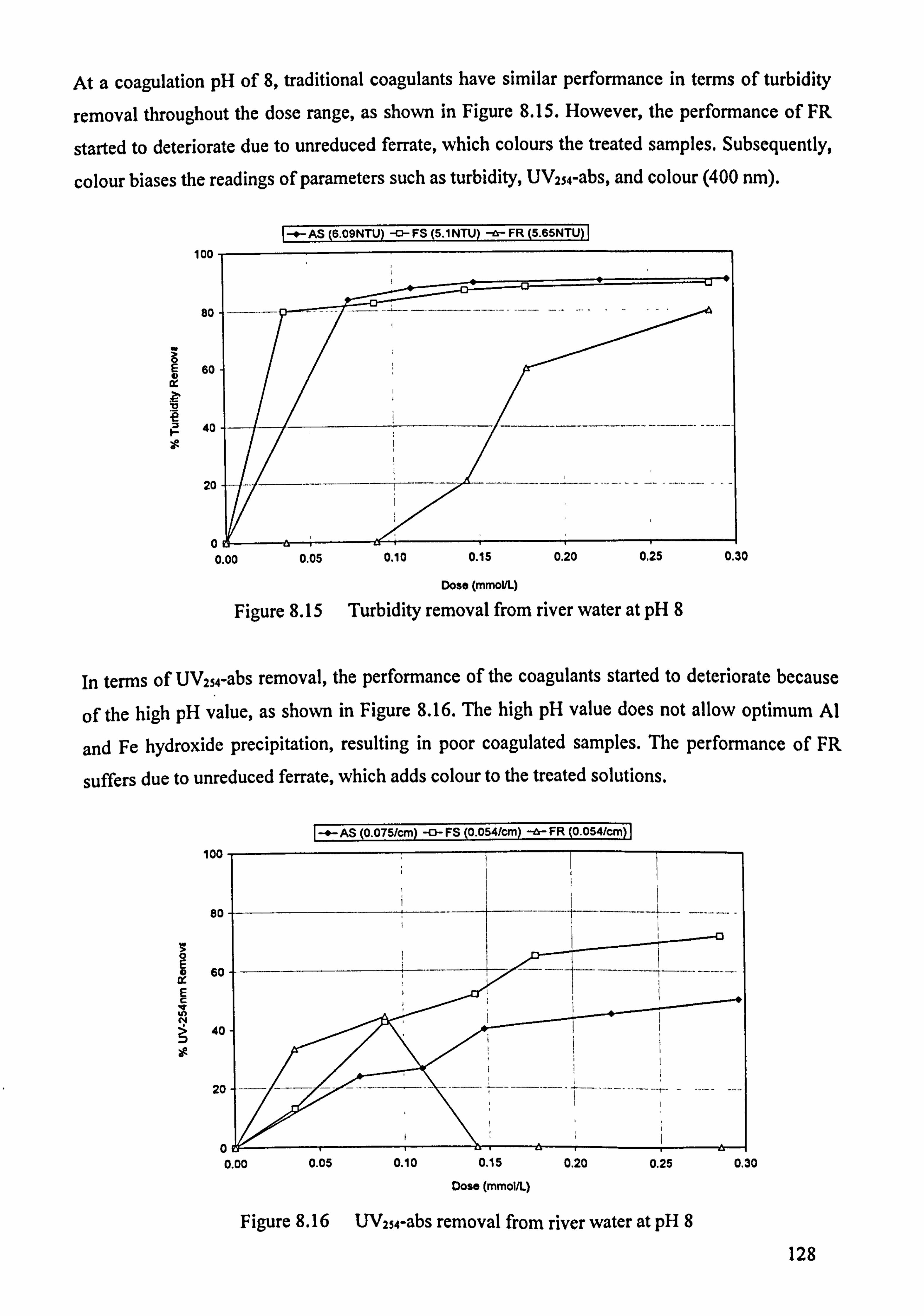
At a coagulation pH of 8, traditional coagulants have similar performance in terms of turbidity
removal throughout the dose range, as shown in Figure 8.15. However, the performance of FR
started to deteriorate due to unreduced ferrate, which colours the treated samples. Subsequently,
colour biases the readings of parameters such as turbidity, UV254-abs, and colour (400 nm).
--#- AS 6.09NTU -C3-- FS (5.1 NTU --&- FR (5.65NTU)
100
80
A 60
40 ä
20
0.00 0.05 0.10 0.15 0.20 0.25
Dose (mmoUL)
Figure 8.15 Turbidity removal from river water at pH 8
0.30
In terms of UV254-abs removal, the performance of the coagulants started to deteriorate because
of the high pH value, as shown in Figure 8.16. The high pH value does not allow optimum Al
and Fe hydroxide precipitation, resulting in poor coagulated samples. The performance of FR
suffers due to unreduced ferrate, which adds colour to the treated solutions.
I-. -AS (0.075/cm) -O-FS (0.054/cm) -6-FR (0.054/cm)
100
80
0 60
c C4 N
40
20
0
i i iý
-- ' -ý---------r-----------ý-- , __ ___. i
i
0.00 0.05 0.10 0.15 0.20 0.25
Dose (mmoWl)
Figure 8.16 W254-abs removal from river water at pH 8
0.30
128

Same as UV254-abs, colour (400 nm) removal of coagulants was started to deteriorate because of
the high pH value, as shown in Figure 8.17. FR did not perform well, as part of ferrate remained
stable at high pH, resulting in colouring of the treated samples.
[-*--AS (0.007/cm) -e-- FS (0.003/cm) -a- FR (0.005/cm
100
80
E 60 d
0 0 40
20
V
0 0.00 0.05 0.10 0.15 0.20 0.25 0.30
Dose (mmolL)
Figure 8.17 Colour (400nm) removal from river water at pH 8
Despite of the colouring problems, FR still achieved completely bacteria inactivation throughout
the dose range, again due to its high redox potential, as shown in Figure 8.18. Once more, the
inactivation performance of traditional coagulants was similar to their turbidity performance, as bacteria removal is believed to be associated with flocs entrapment.
It AS (80000) -o- FS (70000) -A- FR (205000)1
100
80
60
.Q V 40
F-
20
0.00 0.05 0.10 0.15 0.20 0.25 0.30
Dose (mmovL)
Figure 8.18 Bacteria inactivation from river water at pH 8
0
129
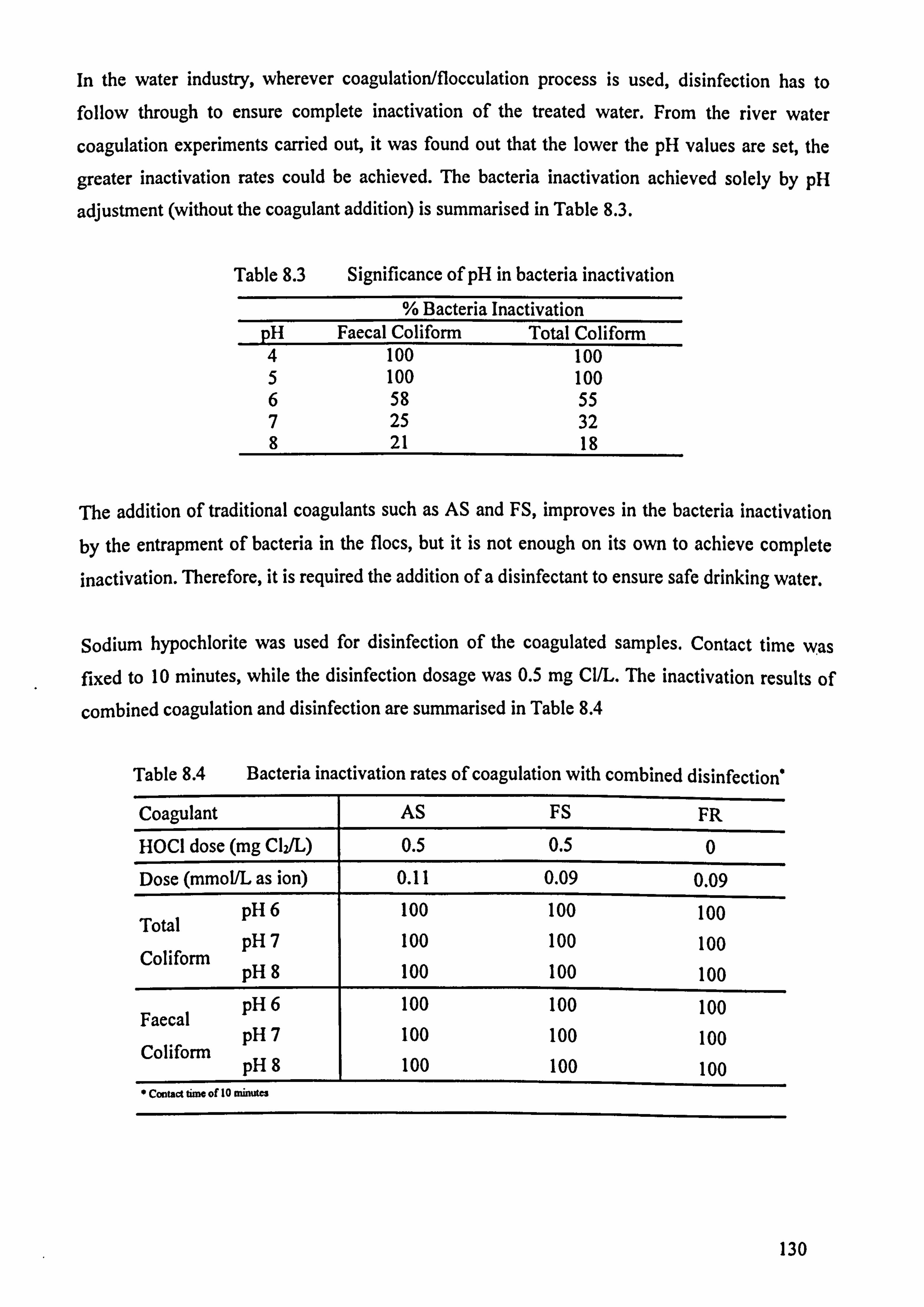
In the water industry, wherever coagulation/flocculation process is used, disinfection has to follow through to ensure complete inactivation of the treated water. From the river water
coagulation experiments carried out, it was found out that the lower the pH values are set, the
greater inactivation rates could be achieved. The bacteria inactivation achieved solely by pH
adjustment (without the coagulant addition) is summarised in Table 8.3.
Table 8.3 Significance of pH in bacteria inactivation
% Bacteria Inactivation pH Faecal Coliform Total Coliform 4 100 100 5 100 100 6 58 55 7 25 32 8 21 18
The addition of traditional coagulants such as AS and FS, improves in the bacteria inactivation
by the entrapment of bacteria in the flocs, but it is not enough on its own to achieve complete
inactivation. Therefore, it is required the addition of a disinfectant to ensure safe drinking water.
Sodium hypochlorite was used for disinfection of the coagulated samples. Contact time was fixed to 10 minutes, while the disinfection dosage was 0.5 mg Cl/L. The inactivation results of
combined coagulation and disinfection are summarised in Table 8.4
Table 8.4 Bacteria inactivation rates of coagulation with combined disinfection'
Coagulant AS FS FR
HOCI dose (mg C12/L) 0.5 0.5 0
Dose (mmol/L as ion) 0.11 0.09 0.09
pH 6 100 100 100 Total
pH 7 100 100 100 Coliform
pH 8 100 100 100
pH 6 100 100 100 Faecal
pH 7 100 100 100 Coliform
pH 8 100 100 100 0 Contact time of 10 minutes
130

8.4 Discussion
The use of FR for coagulation/flocculation and disinfection of river water gave promising results
for its possible future use in water industry. The performance of FR was studied in a wide pH
values, ranging from 4 to 8. As both a coagulant and a disinfectant, FR produced very good
quality of final water for some conditions (pH 6 and 7, and dose 0.18 mmol Fe/L), in terms of
better UV254-abs and colour removal, as well as based on achieving completely bacteria
inactivation. However, final chlorination of the treated water should be still applied even when
there is no bacteria present in the water, in order to provide protection from further
contamination in the distribution network.
The multi-function of FR as a coagulant and a disinfectant makes it a very attractive solution for
the water industry, as in a single sedimentation chamber, coagulation/flocculation and
disinfection can take place, and chlorine demand can be dramatically reduced to a minimum just
to ensure chlorine residual. The overall performance of three coagulants in terms of the removal
of turbidity, UV254-abs, colour (400 nm), and bacteria inactivation (total coliform), and at pH 6
and 7, is summarised in Table 8.5.
Table 8.5 Comparative removal efficiency of turbidity, UV254, colour and bacteria at pH 6 and 7
Optimum doses Removal efficiency
(mmol/L as ion) (%)
Coagulant pH 6 pH 7 Turbidity UV254-abs Colour (400 nm) Bacteria
AS 0.15 0.15 84-90 55-75 83-100 70-93
FS 0.18 0.18 46-90 32-86 25-100 26-98
FR 0.18 0.18 57-90 69-91 100 96-100
Coagulation pH values lower than 6 are most of the time unrealistic in the water industry as too
much acid and base are required for pH adjustments. At pH values of 6 and 7, potassium ferrate's
performance is optimum in terms of turbidity, Wzsa-abs, colour (400 nm) removal, as Fe
hydroxides species can predominate over other complex ions, which do not promote overall
coagulation.
For pH values higher than 7, the performance of potassium ferrate deteriorates due to unreduced
ferrate, which colours the samples. Therefore, pH adjustments to values lower than 8 are crucial
for optimum results in the case of ferrate use. However, the disinfection performance of ferrate is
sustained independent of pH value.
131

Domestic and industrial uses of water generally produce deterioration in quality, and in most
instances, wastewater must be collected and given effective treatment before being released to
the environment. Wastewater usually contains most of the constituents of the water supplied to
an area with additional impurities from local waste-producing processes.
Contaminants may be present as large suspended solids, small suspended and colloidal solids,
dissolved organic and inorganic solids, dissolved gases, immiscible liquids and heavy metals.
Many impurities in wastewater are present as colloidal particles, which do not readily settle and
need to be agglomerated by coagulation and flocculation before they can be settled out, as shown
in Table 9.1.
Table 9.1 Enhanced removal of suspended solids (Metcalf and Eddy, 1991)
Chemical Primary sedimentation tanks
precipitation without the addition of chemicals Suspended solids 80-90% 50-70%
BOD5 50-80% 25-40% Bacteria 80-90% 25-75%
In the first part of this Chapter, the wastewater characteristics and experimental set-up are briefly
outlined. In the second part of this Chapter, the coagulation and disinfection performance in
treating wastewater are presented and discussed. In the third and final part, sludge production in
the process is compared using Imhoff cones method.
9.1 Wastewater
Wastewater samples were collected from the Manor Farm Road Sewage Treatment Works of
Thames Water in Reading. All wastewater samples were obtained from the plant influent prior to
the primary grit chamber. 132

Samples were collected in high density polyethylene (HDPE) jerricans, which were washed and
rinsed with tap water before use. There is a variation in the values of the parameters as a result of'
either the time of sampling or even of the day of the week, as shown in Table 9.2
Table 9.2 Characteristics of industrial wastewater (Jan-Mar 2003) Parameter Range Mean Value
pH 7.25- 7.88 7.57 Turbidity (NTU) 29.4- 73.3 51.4 Total suspended solids (mg/L) 97 - 303 200 UV254-abs (cm-1) 0.168 - 0.316 0.242
Colour Vis-abs at 400nm (cm-1) 0.011 - 0.041 0.026 Unfiltered COD (mg/L) 353 - 527 464 Filtered COD (mg/L) 154 - 194 174 Total Coliform (per 100 mL) 4x10⁸ - 2.2x 10⁹ 1x10⁹ Faecal Coliform (per 100 mL) 3.3x 10⁸ - 2x 10' 1x10⁹
9.2 Wastewater Coagulation
Standard jar tests were conducted to evaluate and compare the treatment etTectivcncss of
potassium ferrate (FR) with traditional coagulants, ferric sulfate (FS), and aluminium sulfate
(AS); both are the most common chemicals used in wastewater works.
9.2.1 Coagulant Dosage
The selected coagulant doses ranged from 0 to 30 mg/L as ion. Stock coagulant solutions were
prepared at a concentration of 1000 mg/L as ion and the sample volume was 1000 niL. In that
way, there is a one to one (1: 1) correlation between desired coagulant dose and the required
volume of stock solutions. All the coagulants doses are expressed in mmol/L as ion, for the equal
comparison reasons.
9.2.2 Experimental Set-up
In this experiment only the type of coagulant, coagulant dosage, and coagulation pl I are under
investigation. The experimental set-up is addressed in detail as follows:
The type of the coagulant - three coagulants, AS, FS, and FR were used; Coagulation pH - three pH values were examined. For FR, pH 5 and 7, and the pII of
raw wastewater, which varied from 8.09 to 9.07. In the case of AS and FS, pl I was not
adjusted - effluent pH varied from 6.75 to 7.48 depending on the doses, and; Coagulant dose - varied from 0.07 to 0.56 mmol/L as ion, as shown in Table 9.3.
133

Table 9.3 Chemical doses for wastewater coagulation
AS FS FR
(mg Al/L) (mmol A1/L) (rng Fe/L) (mmol Fe/L) (mg Fe/L) (mmol Fe/L) 4 0.15 6 0.11 4 0.07 8 0.30 10 0.18 7 0.13 12 0.44 16 0.29 10 0.18 15 0.56 22 0.39 15 0.27
28 0.50 18 0.32 22 0.39 26 0.46 30 0.54
As before, in all the runs, there was a blank sample in which, there was no coagulant added, but
only with pH adjustment if it was necessary. Upon the coagulant addition, the wastewater was
rapidly mixed at a speed of 400 rpm for a period of one minute and then allowed to flocculate at
a speed of 35 rpm for a period of 20 minutes. After the stirring was stopped, the samples were
allowed to settle down for a period of 60 minutes.
At the end of sedimentation, 100 ml- sample was withdrawn from supernatant and measured for
suspended solids (SS), colour (Visaoo-abs), and bacteria (total and faecal coliforms). The
measurement procedures were the same as previous stated and followed the Standard Methods
(APHA, 1995).
9.3 Wastewater Coagulation Results
The principle indicators used for the evaluation of the effectiveness of the three coagulants in
treating wastewater were SS removal, residual colour (Visaoo-abs), and inactivated bacteria (total
and faecal coliforms).
All the residuals values are calculated based on the measured values of the control samples (no
coagulant addition. only pH adjustment). The pH was adjusted with the addition of either
sulphuric acid or sodium hydroxide.
The abbreviations AS, FS and FR appeared in the graphs, stand respectively for aluminium
sulfate, ferric sulfate and potassium ferrate. The numbers in the brackets indicate the value of the
parameter in question such as SS, colour (Visaoo-abs), faecal coliform and total coliform of' the
control sample (no coagulant addition, only pH adjustment).
134

Instead of using turbidity as an indicator for clarity of the treated samples, SS were measured.
There is a strong positive relation between turbidity and SS: the highest turbidity removal, the
highest SS removal. This trend was found as well to be independent of coagulant used and
coagulation pH.
The actual difference between the two parameters was very small. For the three coagulants and
various pHs, it was established that turbidity readings were a little higher than the readings of SS,
mainly because of the interference of colour on the turbidity. Figure 9.1 shows the positive
relation between turbidity and SS removal for ferrate at pH 5, while Figure 9.2 shows the overall
performance of potassium ferrate at different pH values.
+ Turbidity: 21.3NTU SS: 53mg/L
100
80
100
80
60
40
20
60
40
20
0 -+0 0.00 0.10 0.20 0.30 0.40 0.50 0.60
Dose as ion (in mmol/L)
Figure 9.1 Ferrate performance in terms of turbidity and SS removal at pf 15
-o- no pH adjustment (61 mg/L) -0- pH 5 (53mg/L) -ý pH 7 (76mg/L)
100
80 ý
m 60 0 E
to 40
pH 8.09-9.07 20 s.
0 --A 0.00 0.10 0.20 0.30 0.40 0.50 0.60
Dose as ion (in mmol/L)
Figure 9.2 FR's performance for SS removal at different pHs 135

In case of no pH adjustment, pH varied from 8.09 to 9.07 depending on the dose, due to the high
alkalinity of ferrate. As a result of high pH values, ferrate remains unreduced in solution, leading
to a poor coagulation performance.
In terms of removing colour (Vis4oo-abs), FR's performance was at its best at pl i 7, as Figure 9.3
shows. Once again, when pH was not adjusted, ferrate's performance deteriorated dramatically
because of high pH, leading to unreduced ferrate, which causes mainly colouring problems and
poor production of iron hydroxides.
100
-e
0 E d
E c 0 0 0 0 0 ö 0
80
60
4U
20
0 0.00 010 0.20 0.30
Dose as ion (in mmoVL)
0.40 0.50 0.60
Figure 9.3 FR's performance for colour (Visa)o-abs) removal at different pl is
Due to its high redox potential, FR achieved completely (100 per cent) bacteria inactivation at
pHs 5 and 7. This partly due to the oxidation property of the ferrate, and partly owing to the
entrapment of bacteria by the resulting ferric hydroxide flocs at pH 7.
FR shows optimum performance in terms of SS and colour (Visaoo-abs) removal at a pll 7. This
pH value would be used in order to compare the coagulation performance of three coagulants. In
the case of AS and FS, pH varied from 6.75 to 7.4 depending on the coagulant dose. 'I'his p11
range falls in an area where the maximum Al and Fe hydroxides are formed.
Figure 9.4 shows that SS concentration in control sample for FR test was lower than that for the
tests of AS and FS, thus. FR has a better performance for the SS removal. Nevertheless, this was
a shortcoming as the raw wastewater quality can not be controlled if conducting a site trial.
136
no pH adjustment (0.020/cm) -t-- pH 5 (0.014/cm) -6- pH 7 (0.012/cm)

> 0 E d
FR (76mg/L) AS (99mg/L) - -FS (110mg/L) l
100
80 - pH 6.75-7.48
pH pH 6.75-7.48
60 -
40
20
0 0.00
Figure 9.4
0.10 0.20 0.30 0.40 0.50 0.60 Dose as ion (in mmol/L)
Wastewater coagulation performance in terms of SS removal
Moreover, in terms of removing colour (Visaoo-abs), FR has the best performance as Figure 9.5
shows, about 50% more colour can be removed by FR for the same doses compared. This is
because as a strong oxidant. FR has the capability to reduce organic materials that are responsible
of the colour in wastewater.
100 ý
80
0
60
E c 0 0
40
0 ö U
20
pH 7
pH 6.75.
pH 6.75-7.48
0 0 00 0.10 0.20 0.30 0.40 0.50 0.60
Dose as ion (in mmol/L)
Figure 9.5 Wastewater coagulation performance in terms of removing colour (Vis4oo-abs)
FR not only oxidises organic matter present in wastewater, but can also disinfect bacteria, which
traditional coagulants lack the power to do. At pH 7, FR can achieve completely bacteria
inactivation, while its rivals can remove only a maximum of 91 per cent of bacteria. All the
bacteria results are presented in Table 9.4.
137
-- FR (0.012/cm) -- AS (0.01 O/cm) -c- FS (0.010/cm)
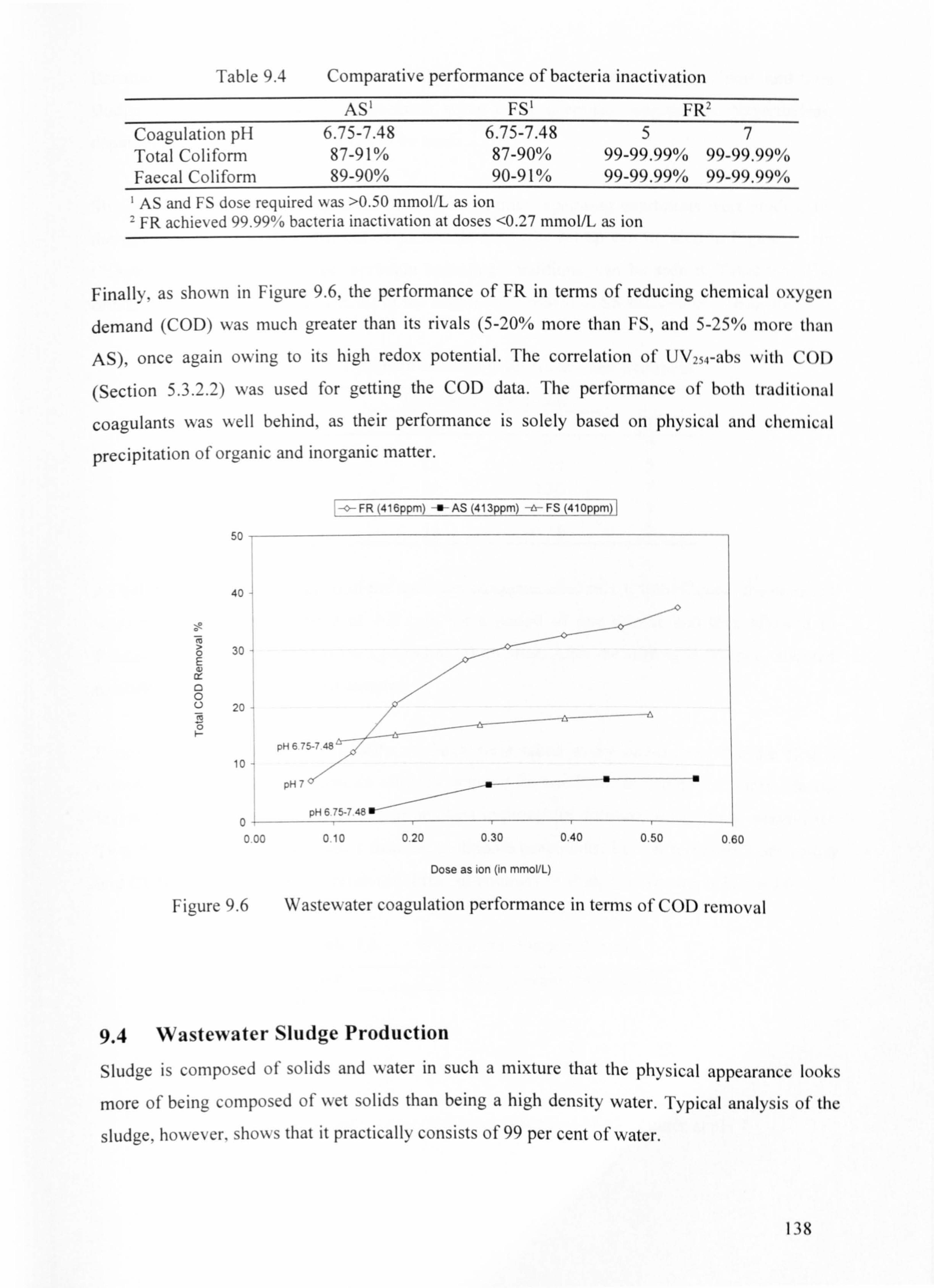
Table 9.4 Comparative performance of bacteria inactivation
AS' FS' FR' Coagulation pH 6.75-7.48 6.75-7.48 57 Total Coliform 87-91% 87-90% 99-99.99% 99-99.99% Faecal Coliform 89-90% 90-91% 99-99.99% 99-99.99%
AS and FS dose required was >0.50 mmol/L as ion 2 FR achieved 99.99% bacteria inactivation at doses <0.27 mmol/L as ion
Finally, as shown in Figure 9.6, the performance of FR in terms of reducing chemical oxygen
demand (COD) was much greater than its rivals (5-20% more than FS, and 5-251/o more than
AS), once again owing to its high redox potential. The correlation of UV254-abs with ('OI)
(Section 5.3.2.2) was used for getting the COD data. The performance of both traditional
coagulants was well behind, as their performance is solely based on physical and chemical
precipitation of organic and inorganic matter.
FR (416ppm) f- AS (413ppm) -ä- FS (4lOppm)
50
40 1
. -I 0 30 E
0 0 U 20 iv 0 H
10 pH67'.
pH 7 -a
0 pH 6.75-7.48 w-
0.00 0.10 0.20 0.30 0.40 0.50 0.60
Dose as ion (in mmol/L)
Figure 9.6 Wastewater coagulation performance in terms of COD removal
9.4 Wastewater Sludge Production
Sludge is composed of solids and water in such a mixture that the physical appearance looks
more of being composed of wet solids than being a high density water. Typical analysis of the
sludge, however, shows that it practically consists of 99 per cent of water.
138

Because the resulting sludge contains of high percentage of water, its large volume and thus
sludge treatment are the biggest drawback when using chemical coagulation. Nevertheless,
depending upon circumstances. it has to be used.
Sludge production and settling speed under the optimum operating conditions were studied by
the use of a cone-shaped vessel called an Imhoff cone (the set-up can be seen in Figure 5.1 in
Chapter 5). The pre-determined, optimum operating conditions, can be seen in Table 9.5. The
criteria for their selection are in terms of the maximum removal of SS and colour (Vis4oo-abs).
Table 9.5 Optimum conditions for wastewater treatment
Coagulant Optimum dose as ion
mg/L mmol/L pH Blank 00 7 AS 10 0.37 7 FS 20 0.36 7 FR, o� 15 0.27 7 FRh,,, h 20 0.36 7
As before, upon the introduction of the optimum coagulant dose in IL Imhoff cone, the contents
were rapidly mixed at a speed of 400 rpm for a period of one minute and then allowed to
flocculate at a speed of 35 rpm for a period of 20 minutes. After the stirring is stopped, allowed
to settle down for a period of 60 minutes.
During the settlement time, turbidity readings were taken every one-minute for the first 5
minutes, and then every 10 minutes until 60 minutes for one hour, as Figure 9.7 shows. In the
legend above the graph, the numbers in brackets indicate the optimum dose of the coagulants.
Two doses of FR performed better than the traditional coagulants, i. e. FR removed more colour
and COD than AS and FS, but produced different volumes of sludge, as shown in Table 9.6.
Table 9.6 Wastewater sludge volumes
Coagulant Sludge production (in mL) Blank 20 AS 40 FS 40 FR,,, � 30 F R,,, F,, 35
Figure 9.7 Turbidity removal during settlement of 60 minutes at pH 7
139

Ctrl -u- AS (10 mg/L) -A- FS (20 mg/L) x FR (15 mg/L) O FR (20 mg/L) j
O
0 E
D
E-
100
90
80
70
60
50
40
30
20
10 {
0Ö 0
Two sources are considered to contribute to the production of sludge: contaminants in the raw
wastewater and the solids produced from the coagulant. The difference of total SS before and
after coagulation should give the coagulant quantity used and the contaminants removed. as
Equation 9.1 and Figure 9.8 show.
[Removed contaminants and coagulant] = SsILldgedeposit - SSRaw - SSI111h ff 1.1IU lt1 011 9. I
Where: SS Sludge deposit is SS in the bottom of Imhoff cone after coagulation and sedimentation SSRaw is SS of the raw wastewater prior to coagulation and sedimentation SSI,,, hOnf is SS remained in the Imhoff cone after coagulation and sedimentation
SSlmhoa- Unsettled SS after chemical coagulation
ýI:
. 4- -- SSsiudgedeposit (Sludge from SSRa, ) + (Sludge From coagulant)
Figure 9.8 Schematic representation of mass balance after chemical coagulation
14()
10 20 30 40 50 60
Settling time (in minutes)

The right part of Equation 9.1 can be measured by the SS method when using Imhol, f cone. Once,
all the SS measurements are completed, then the coagulant contribution into sludge mass can he
calculated, as Table 9.7 shows.
Table 9.7 Mass balance of wastewater coagulation
Raw Imhoff Sludge C'oagulant'
De osit /L mL 9 mL
AS 0.3820 0.0364 960 0.47 40 0.0516 FS 0.3820 0.0204 960 0.49 40 0.0876 FR, O�.. 0.3820 0.0335 970 0.51 30 0.0945 FRh gh 0.3820 0.0285 965 0.54 35 0.1295 ' Coagulant = Raw- [lmhoft + Sludge]
At both doses, low and high (15 and 20 mg Fe/L respectively), FR manages to produce a better
quality sludge not only in terms of volume, less than 40 nit., but the most important in tcrins of
sludge density, as Table 9.8 shows.
Table 9.8 Sludge density
Coagulant Density (in nig/mL) AS 11.8 FS 12.3 FR (low) 17.0 FR (high) 18.3
Therefore, the sludge produced by potassium ferrate is considerable less in volume than AS and
FS. Nonetheless, ferrate's sludge is easier to treat, therefore making its treatment an attractive and
cost effective for wastewater operators.
9.5 Discussion
The use of FR for coagulation/flocculation and disinfection of wastewater gave very promising
results for its possible future use in water industry. As a coagulant, FR produced very good
quality of final water comparing that of traditional iron and aluminium coagulants produced.
In addition to this, potassium ferrate acts as an oxidant reducing organic matter. Moreover, as a
disinfectant, FR produced very high quality of final water, achieving complete bacteria
inactivation, due to its high redox potential. However, potassium ferrate does not provide any
form of residual as chlorine disinfectant does. 1-31

The multi-function of disinfection and coagulation makes FR a very attractive solution for
wastewater industry. FR's performance in terms of SS removal, colour (Visaoo-abs) removal, and bacteria inactivation, is summarised in Table 9.9.
Table 9.9 FR's performance for wastewater coagulation as % removal
pH SS Colour (Visaoo-abs) Bacteria inactivation
5 13-72 42-100 99-99.99
7 67-91 60-100 99-99.99
The optimum pH for wastewater coagulation was found to be at pH 7, because all added ferrate
could be reduced to ferric ions and subsequently optimum iron hydroxides were produced,
enhancing the coagulation/flocculation.
In the case of no pH adjustment, FR's performance deteriorated dramatically because of
unreduced ferrate, which it just coloured the solution and it did not produced any ferric ions. The
comparative performance of three coagulants at optimum pH is summarised in Table 9.10.
Table 9.10 Comparative performance of coagulants at optimum dose
AS FS FR pH 6.75-7.48 6.75-7.48 5 7 Optimum dose as ion (in mg/L) 8 22 15 22 Optimum dose as ion (in mmol/L) 0.30 0.39 0.22 0.39 Suspended solids removal (%) 91 95 80 88 Colour (Visaoo-abs) removal (%) 50 50 100 92 Total COD removal (%) 7 18 43 32 Bacteria inactivation (%) 90 91 99+ 99+
Finally, FR's performance is outstanding as well in terms of sludge production, as it can produce
not only less volume, but also high sludge density, which makes sludge treatment to be easier. The exceptional multi-function of ferrate and its superior performance in wastewater treatment
were confirmed in the study.
142

Iý 1YýýY
JJL1/
In previous Chapters, potassium ferrate (FR) showed great potential as a coagulant, oxidant and
disinfectant when different types of waters were treated with ferrate. In order to use it fully, it is
essential to evaluate its stability, which is one of very important fäctors to affect the efficient use
of a chemical in water and wastewater treatment.
This Chapter studies the impact of different factors on the stability of' tcrrate products. it is
obvious that the resulting ferrate products should be stable if the preparation temperature can be
controlled as low as possible and the alkalinity and/or pH of the products can he nfaiiitaineti
greater than 8.
The decomposition rate of ferrate depends on the purity of the product, initial Icrratc
concentration, pH, co-existing ions, and temperature. A full understanding of the impacts of
these factors on the stability of ferrate is important to assess the future viability of the product in
the water and wastewater industry.
10.1 Stability of Ferrate Salts
When ferrate salts are dissolved in water, the ferrate ion undergoes decomposition N%ith the
evolution of oxygen as shown in Equation 10.1. The lowest rate of reduction o1' potassium Icrratr
by water occurs between pH 9.4 and 9.7 (Lee and Gai, 1993).
4K2FeO4 + 4H20 - 2Fe2O3 + 8KOH + 3021 Equation 10.
143

10.2 Experimental Design
Solid potassium ferrate with 6 per cent purity was prepared by the modified chlorine method as described in Chapter 5. Fe (VI) product is evaluated for its stability not only as a solid, but also
as well in solution by dissolving solid samples of K2FeO4 into KOH solutions. All samples were
measured for their stability using the spectroscopy method at a wavelength of 504 nm.
Solid Fe (VI) is split in four parts, each one subjected to different environment conditions. One
part is kept in the freezer, the second part on the bench in direct contact with air, the third part in
a sealed tube placed in a desiccator, and the fourth part in a sealed tube placed only in a dark
place in the laboratory.
The Fe (VI) solutions were prepared by addition of solid samples of K2FeO4 to 1M and 3M KOI 1,
where solutions are most stable, from hours to weeks (Stuart et al., 1999). The concentration of
Fe(VI) solutions was in all cases 0.005M as ion. In addition, Fe (VI) solutions were prepared by
addition of solid samples of K2FeO4 to deionised water and a 0.05M nitrate to investigate the
effect of the co-existing ions on the ferrate stability at a constant temperature of 200 C. Figure
10.1 shows in detail all the experiments carried out for the stability evaluation of Fe (VI).
Ferrate (VI)
Solid (6% purity) Solution (0.005M as ion)
Sealed Sealed Open Freezer KOH Deionised Deoinised water and Dark Desiccator air 1,3M water NO3 (0.05M)
Figure 10.1 Stability evaluation experimental design
10.3 Stability Results
Most of the results presented in this part agree with the findings of other researchers. HHowever,
there are some exceptions, mainly due to the low purity (6%) of the products compared to the high purity products referred in the literature (98+%). The solid ferrate products used in the study
contain large impurities of excess hydroxide, chloride, and ferric hydroxide, which may
accelerate the decay of the ferrate ion.
144

Figure 10.2 shows the stability of an open air sample at a constant temperature of 200 C. It was found that the ferrate ions decomposed rapidly in the initial stage and found to be relatively
stable for a maximum of approximately 2 weeks. The moisture present in the air is the main
reason causing Fe (VI) decay.
6
5
c c
ä3
d 2
1
o+ 0
I
I
I
i
_. ... _. _ý... ý_. ý
I, I
iI
ý
....... .. I
.......... _i. . «»..
1
'
123456789 10 11 12 13
Time (in days)
Figure 10.2 Stability of solid Fe (VI) sample exposed in open air
On the other hand, solid samples in sealed bottles were found stable at a constant temperature of
200 C. The isolation of the samples from direct contact with air extends their life significantly for
a period of more than 4 months.
Furthermore, it was found that solid samples kept in the freezer were stable for more than 12
months. For the case of the industry, this means that special storage rooms with freeze facilities
should be provided for keeping stocks of the product, making this solution uneconomical.
Figure 10.3 shows that the sealed sample kept in the desiccator was slightly more stable than the
sealed sample kept in the dark, primarily because the extra layer of protection provided by the
desiccator, which guaranteed complete dry conditions. This is evidence that only moisture affects
the stability of the sample and not exposure to light, which is consistent with previous studies
(Wagner et al., 1952).
145
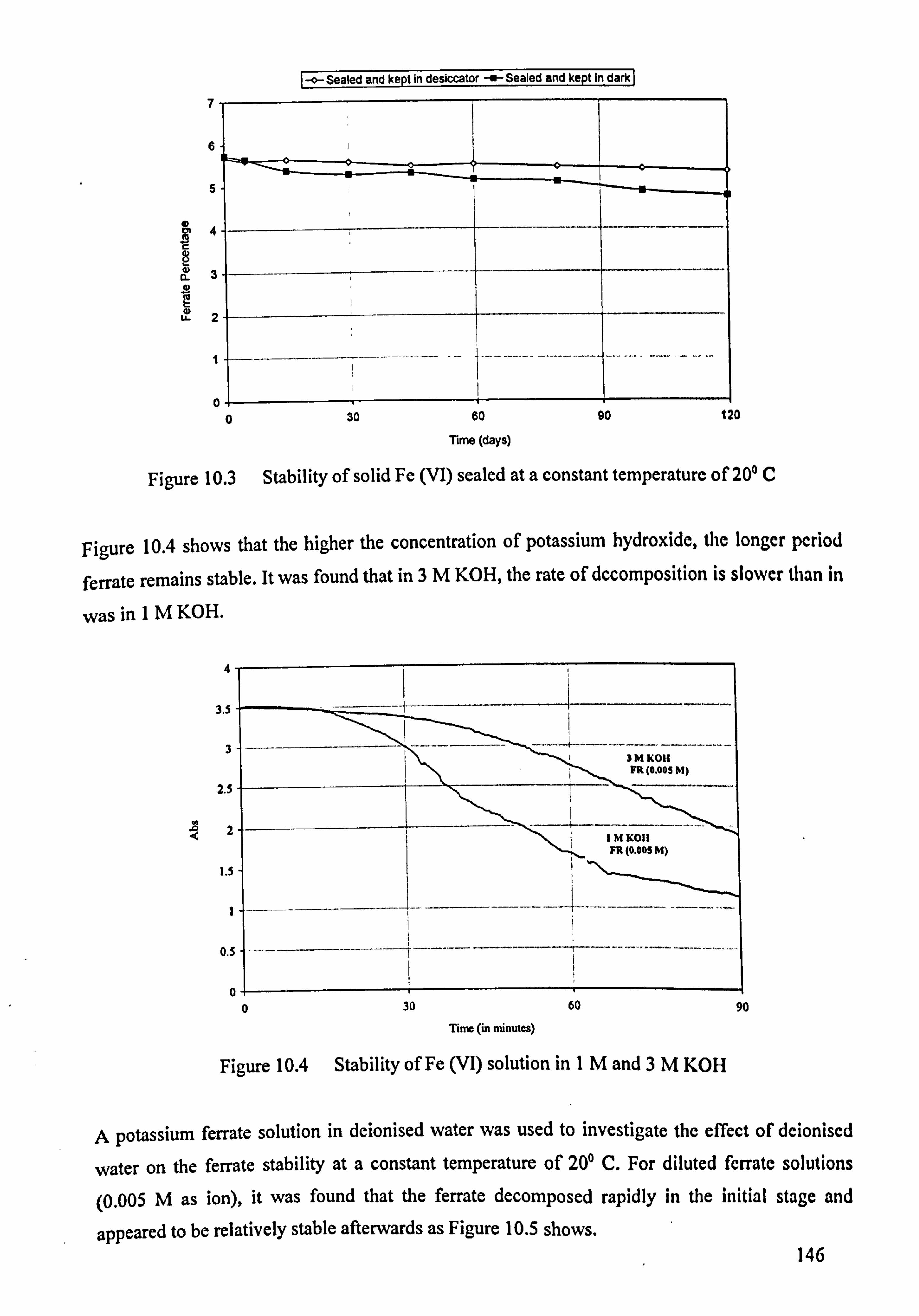
-o-Sealed and kept in desiccator -a-Sealed and kept In dark
7
6
5
4 c
CL
u2
1
Time (days)
Figure 10.3 Stability of solid Fe (VI) sealed at a constant temperature of 20° C
Figure 10.4 shows that the higher the concentration of potassium hydroxide, the longer period
ferrate remains stable. It was found that in 3M KOH, the rate of decomposition is slower than in
was in 1M KOH.
4
3.5
3
2.5
2
1.5
I
0.5
3M KOH FR (0.005 M)
IMKOII FR (0.005 M)
i
0 30 60 90
Time (in minutes)
Figure 10.4 Stability of Fe (VI) solution in 1M and 3M KOH
A potassium ferrate solution in deionised water was used to investigate the effect of dcioniscd
water on the ferrate stability at a constant temperature of 20° C. For diluted ferrate solutions
(0.005 M as ion), it was found that the ferrate decomposed rapidly in the initial stage and
appeared to be relatively stable afterwards as Figure 10.5 shows. 146

This can be explained because all Fe (VI) has been already reduced to Fe (III), which in turn
interferes with the optical monitoring of the reaction until it is completely precipitated out of
solution.
4
3.5
3
2.5
2 ýe I
1.5
0.5
0
FR (0.005 M)Ie Nitrate (0.05M)
FR (0.005 M) DI water
FR (0.005 M) in Im k011 i
1
0 20 40 60 80 100
Time (in minutes)
Figure 10.5 Effect of deionised water with/without nitate ion on Fe (VI) stability
When nitrate was added in ferrate solutions, it was found that ferrate was stable for longer time.
This is because co-existing ions are served as a complexing agent for Fe (VI) reducing its
precipitation rate out of solution.
10.4 Conclusions
The stability evaluation of the solid ferrate products gave promising results. In future, the use of
ferrate salt in full-scale water and wastewater treatment is viable, providing that the products are
not only of high purity, but also stable for long period prior to use.
In this study, a long stable period was observed of ferrate solids kept in either low temperature
(00 C) or in a sealed contained in the desiccator. Light was found not to have any significant
effect on the stability of solid products. For a commercial use ferrate salts should be packed in
airtight containers to prevent product decay.
For ferrate solutions, it was found that their stability increases with increasing alkalinity. In
addition, ferrate in deionised water decays rapidly, while when nitrate ion was added, ferrate
remained stable for longer period. 147

Potassium ferrate in this study was prepared by a wet method where iron (111) was oxidised in a
strong basic solution by potassium hypochlorite to form ferrate(VI) ions. The perliýrniancc uI-the
resulting ferrate in wastewater and water treatment was evaluated and compared with that (it'
conventional coagulants (aluminium sulfate and ferric sulfate) and disinfectant (chlorine). 'I lir
findings of this study can be summarised and seen in the following sections.
11.1 Potassium Ferrate Synthesis
Two routes of synthesis to the formation of potassium ferrate were trial. either using a
commercial available sodium hypochlorite solution with the strength of approximately 12°',
available chlorine (-120 g/L) as the oxidant, or using a modified chlorine method where a high
strength hypochlorite solution [40 to 50% as the available chlorine (400-S00 g/L)j \\as first
prepared and used as the oxidant to form ferrate (VI).
All attempts to produce the potassium ferrate using commercial sodium hypochloorite t'aiIcil
principally because of its low hypochlorite concentration.
A concentrated strongly alkaline solution of potassium hypochlorite was first generated by
bubbling chlorine gas into cold, aqueous analytical grade potassium hydroxide. 'Technical grade
potassium hydroxide was tried as well but it produced a lot of precipitates. The chlorine gas was
generated by dropping concentrated hydrochloric acid on potassium permanganate.
A ferric nitrate concentrated solution was added into the resulted concentrated pol'ISS1,11111
hypochlorite (42-44%) solutions. The suspension was mixed for one hour at temperature oI' less
than 10° C and the mixtures were filtered to examine the ferrate solid formed. Ferric sulläte as
tried as well but it did not produce solid ferrates.
i4K

The molar ratio of chlorine to iron was then investigated, and it was found that a molar ratio of C1: Fe of 10 to 1 gave not only the highest ferrate concentration (0.33 mol/L), but also it achieved
the highest yield (19.64%).
This study aims to prepare crude ferrate (6% purity) in order to reduce the preparation cost, thus,
centrifugation and freeze-dry techniques were used to separate solid ferrate (12 g per 50 mL hypochlorite solution) from the mixtures.
The products from the chlorine oxidation of ferric salt were centrifuged at 4500 rpm for 14
minutes. The liquid phase was discarded, while the solid phase was put for freeze-dry at -58° C
for a minimum period of 24 hours. The products from that process were completely in solid
form, that was easily grounded in a mortar to powder form. A summary of the preparation
conditions of potassium ferrate is given in Table 11.1.
Table 11.1 Potassium ferrate's preparation conditions using chlorination method
Process Conditions Time (hh: min) Potassium hypochlorite synthesis Ice bath, stirring 01: 30
Addition of excess KOH Ice bath, stirring 01: 00
Ferric nitrate addition Ice bath, stirring 01: 00
Centrifugation 4500 rpm 00: 14
Freeze-dry -58°C 24: 00
H. 2, Potassium Ferrate Stability
Stability tests carried out in this study using solid samples of potassium ferrate (6% purity) show
that the products are stable either when stored in low temperature (_< 00 C) or in a moisture free
environment, as air will decompose the ferrate to ferric. For a commercial use, crude ferrate salts
could be packed in airtight containers.
On the other hand, when ferrate is in a high alkalinity solution (3M KOH), it was more stable than lower alkalinities. As far it concerns the co-existing ions, nitrate was shown to retard the ferrate decomposition significantly.
149

Longer stability periods should be expected for ferrate sample of higher purity than the oncs
prepared and used in this study. However, the high costs required for the purification would
block the use of ferrate in practice.
11.3 Water and Wastewater Treatment by Potassium Ferrate
Tests carried out in this study using potassium ferrate (FR) show that it is a good water treatment
reagent for the removal of turbidity, colour, COD, and inactivation of bacteria. In all casts, FR
produced high quality of final water, predominately due to its simultaneously action as an oxidant, coagulant, and disinfectant.
In treating university lake water at pH 7.5, FR was capable to inactivate the bacteria at a range of
90 to 96 per cent for a minimum dose of 0.5 mg Fe/L and for any given contact time, which was
much greater than that the chlorine based disinfectant could achieve at relatively high dosages e. g
more than 2 mg Cl/L. Moreover, FR produced the 50-65 per cent less sludge volume than
traditional coagulants, which could reduce significantly the overall sludge treatment costs, and
hence, favoured its use in the industry.
In treating model coloured water, FR achieved a good colour (UV254-abs) removal, although FS
performed better than both AS and FR. Control of coagulation pH is important, as it affects both
the coagulating species and the level of dissociation of humic acids.
In treating natural river water, the FR produced very high quality of final water at pH values of 6
to 7 and doses of 0.18 mmol Fe/L. Comparing with AS and FS, the FR can achieve completely
colour (Visaoo-abs) removal at lower dose of 0.04 mmol Fe/L, and completely bacteria
inactivation for the doses as low as 0.09 mmol Fe/L.
In treating wastewater, FR produced once more better quality of final water, comparing that of
traditional iron and aluminium coagulants produced. FR was capable to remove more than 40 per
cent of COD at a dose of 0.22 mmol Fe/L and at a pH 5, which was much greater (2 to 7 times)
than the traditional coagulants could achieve at given dose (0.07 to 0.56 mmol/L as ion).
For the inactivation of bacteria and the sludge production, FR achieved 99-99.99 per cent
inactivation of bacteria and 25 to 30 per cent less sludge than AS and FS, and the resulting
sludge had high density and smaller water content.
ISO

11.4 Summary
Crude potassium ferrate samples can be produced and used successfully in the treatment of water
and wastewater, and this has been confirmed in this study. The low purity does not affect FR's
stability provided it is stored either in low temperature environment or air isolated container.
Working as a disinfectant, FR achieves an outstanding inactivation performance compared to the
traditional chemicals used as disinfectants (chlorine). Its disinfection performance is sustained
independent of pH under studying conditions. However, FR does not provide the desired residual
as chlorine based disinfectants do, which is essential for preventing potable water contamination
in the distribution network, and hence chlorination would be still required in some cases, but in
lower doses than the ones applied today in the industry.
Working as a coagulant, FR produces good quality of final water in all the cases, similar to that
of traditional iron and aluminium coagulants (AS and FS) based on turbidity removal, but much
better than AS and FS in terms of colour and organic removal, but this requires rigorous p! i
control, FR preferably works at pH 6 and 7.
The advantages of using FR can be summarised as a better disinfection and coagulation
performance, less sludge production, as well as a single mixing dosing and mixing unit process
could be applied, these should make the use of FR as a chemical to be very promising in both
water and wastewater industries.
11.5 Future Work
it is important that an economic method of synthesising FR in large quantities has to be
investigated, if ferrate should be used in water and wastewater industry successfully.
Once crude ferrate can be produced in large quantities economically, then the performance of
ferrate should be extensively tested in a pilot scale plant for both water and wastewater treatment.
Except for all the parameters studied (turbidity, colour, UV2s, -abs, bacteria, COD, and sludge
production), further evaluation of the FR performance should target to range of organics and
other microorganisms such as cryptosporidium. In addition, systematic studies should be
conducted to confirm that there are no mutagens produced in treating different types of water
with ferrate (VI).
151

References

-A- Akesson, G. and Hongve, D., 1996. Spectrophotometric determination of water colour in I lazcn
units. Water Research, 30 (11), pp. 2771-5.
American Public Health Association (APHA), 1995. Standard Methods for the Examination of Water and Wastewater, 19th ed., Washington DC.
American Water and Wastewater Association (AWWA), 1996. Water Transmission and Distribution. AWWA, Denver.
Arslan, M., Alkan, C. and Cici, M., 1994. Production of Fe203 from FeSO4xII2O formcd in
Galvanising Works Resources. Conservation and Recycling (73): 341-7.
-B- Bartzatt, R.. L, 1982. The Kinetics of Oxidation of Various Organic Substrates by Potassium Fcrratc,
PhD Thesis, University of Nebraska.
Bartzatt, R. L. and Carr, J., 1986. The Kinetics of Oxidation of Simple Aliphatic Sulfur-Compounds
by Potassium Ferrate. Transition Metal Chemistry, 11(3): 116-117.
Bartzatt, R. L., and Nagel, D., 1991. Removal of Nitrosamines from Waste-Water by Potassium
Ferrate Oxidation. Archives of Environmental Health, 46(5): 313-315.
Bartzatt, R. L., Cano, M., Johnson, L. and Nagel, D., 1992. Removal of Toxic Metals and Nonmetals from Contaminated Water. Journal of Toxicology and Environmental Health, 35(4): 205- 210.
Behl, S., Moudgil, M. and Prakash, T. S., 1993. Control of active sites in selective flocculation. Journal of Colloidal and Interface Science, 161: 414.
Bolto, B. A. and Spurling, T. H., 1991. Water Purification with Magnetic Particles. Environ. Monitor. Assess., 19: 139-143.
Bouzek, K., Lipovska, M., Schmidt, M., Rousar, I. and Wragg, A. A., 1998. Electrochemical
production of ferrate(VI) using sinusoidal alternating current superimposed on direct current: grey and white cast iron electrodes. Electrochimica Acta, 44(4), pp. 547-557.
Bratby, J., 1980. Coagulation and Flocculation with an emphasis on water and wastewater treatment. Upland Press, Croydon.
Buffle, J., 1988. Complexation Reactions in Aquatic Systems: an Analytical Approach. liorwood,
Chichester, UK.

-c- Caddick, S., Murtagh, L. and Weaving, R., 2000. Potassium ferrate on wet alumina: Preparation and
reactivity. Tetrahedron, 56(47), pp. 9365-9373.
Carrington, A., Schonland, D. and Symons, M., 1957. Structure and Reactivity of the Oxyanions of
Transition Metals. Part IV. Some Relations between Electronic Spectra and Structurc. J.
Chem. Soc., pp. 659-65.
Cici, M. and Cuci, Y., 1997. Production of some coagulant materials from galvanizing workshop
waste. Waste Management, 17(7), pp. 407-410.
Cotton, F. A. and Wilkinson, G., 1999. Advanced Inorganic Chemistry, 611 Edition. John Wilcy and Sons, New York.
Crozes G., White P. and Marshall M (1995) Enhanced Coagulation: its Effect on NOM Removal
and Chemical Costs. J. AWWA 87 (1): 78-89.
-D- f
Delaude, L. and Laszlo, P., 1996. A novel oxidizing reagent based on potassium ferrate(VI). Journal
of Organic Chemistry, 61(18): 6360-6370.
Deluca, S. J., Cantelli, M. and Deluca, M. A., 1992. Ferrate Vs Traditional Coagulants in the Treatment of Combined Industrial Wastes. Water Science and Technology, 26(9-11): 2077-
2080.
DeLuca, S. J., Chao, A. C., and Smallwood, Jr., C. 1983. Removal of Organic Priority Pollutants by Oxidation-Coagulation. J. Environ. Eng., 109,36.
Dobbs, R. A., Wise, R. H. And Dean R. B. 1972. The use of UV absorbance for monitoring the TOC
of water and wastewater. Water Research, 6, pp. 1173-1180.
-E- EC, 1998. EC Drinking Water Directive 98/83/EEC, EC, Luxembourg.
Eckenfelder, W. W., 2000. Industrial Water Pollution. McGraw-Hill, New York.
Eddy, M. A., 1991. Wastewater Engineering. McGraw-Hill, New York.
Edzwald, J. K. , 1979. Coagulation of Humic Substances. AIChe Sym. Series 190, Watcr-1979,
75: 54.

Edzwald, J. K., Becker, W. C., Wattier, K. L., 1985. Surrogate Parameters for Monitoring Organic
Matter and THM Precursors. J. AWWA, (4): 122-132.
-F- Fair, G. M., 1971. Elements of Water Supply and Wastewater Disposal, New York.
Firouzambadi, H., Mohajer, D., Entezari-Moghaddam, M., 1986. Barium Ferrate Monohydratc: a
versatile reagent for oxidation of organic compounds under aprotic condition. Synth.
Commun. 16,723-731.
-G- Gallerani, P. and Drake, D., 1993. Wastewater Management for the Metal Finishing Industry in the
21st Century. Plat. Surf. Finish, 80(10).
Gilbert, M. B., Waite, T. D. and Hare, C., 1976. Analytical Notes: an investigation of the applicability
of Ferrate Ion for disinfection. AWWA: 495-497.
Dingell, R., Wallcave, R. and Nagel, D., 1976. Metabolism of the Pancreatic Carcinogen N-
Nitrosobis 2- Oxopropyl Amine and N-Nitrosobis 2-Hydroxypropyl Amine in the Syrian
Hamster. J. Nat. Cancer Inst., 57: 1175-1178.
Goff, H. and Murmann, RK., 1971. Studies of the Mechanism of Isotopic Oxygen Exchange and Reduction of Ferrate (VI) Ion. J. Am. Chem. Soc., 93: 6058-6065.
Gray, N. F., 1999. Water Technology. Arnold, London.
Griffith, W. P., 1966. Infrared Spectra of Tetrahedral Oxyanions of the Transition Metals. J. Am.
Chem. Soc., 10: 1467-1468.
Gritter, R. J., Dupre, G. D. and Wallace, T. J., 1964. Oxidation of Benzyl Alcohols with MnO2. Naturc
(202): 179-181.
Gump, . J. R., Wagner, W. F., Schreyer, J. M., 1954. Preparation and Analysis of Barium Ferrate (VI).
Anal. Chem. 26,1957.
Gurol, M. D. and Bremen, W. M., 1985. Oxidation of Cyanides in Industrial Wastewaters by Ozonc.
Environ. Progress, 4(1): 46-51.
-H- Haire, G. R., 1965. A Study of the Decomposition of Potassium Ferrate (VI) in Aqueous Solution,
PhD Thesis, Michigan State University.

Hanewald, R. H., 1985. Recovery of Metals from Steel Wastes and Production of DRI by the INMETCO Process. Iron and Steel Engineer, 62(3): 62-7.
Hoppe, M. L., Schlemper, E. O. and Murmann, R. K., 1982. Structure of Dipotassium Ferrate (VI).
Acta Crystallographica(B38): 2237-2239.
Housecroft, C. E. and Sharpe, A. G., 2001. Inorganic Chemistry. Prentice Hall, London.
Howard, W. A. and Parkin, G., 1994. Terminal Oxo, Sulfido, Selenido and Tellurido Complexes of Zirconium: Comparison of Terminal Zr-E Single and Zr=E Double Bonds Lengths. J. An Chem. Soc., 116(2): 606.
Hrostowski, H. J. and Scott, A. B., 1950. Magnetic Susceptibility of K Ferrate. Chem. Phys. (18): 105- 107.
-J- Jacangelo, J. G., DeMarco, J., Owen, D. M., Randtke, S. J., 1995. Selected Processes for Removing
NOM: an Overview. J. AWWA, 87: 64-77.
Jia, H. D., Yang, X. L., Yang, Y. and Gao, Y. F., 1999. Direct spectrophotometric determination of ferrate(VI). Chinese Journal of Analytical Chemistry, 27(5): 617-617.
Jiang, J. Q. and Lloyd, B., 2002a. Progress in the development and use of ferrate(VI) salt as an oxidant and coagulant for water and wastewater treatment. Water Research, 36(6): 1397- 1408.
jitsuhiro, S., Nakai, M., Hada, M. and Nakatsuji, H., 1994. Theoretical Study on the Ground and Excited States of the Chromate Anion CrO4-2. Chem. Phys., 101(2): 1029.
Johnson, M. D. and Read, J. F., 1996. Kinetics and mechanism of the ferrate oxidation of thiosulfate
and other sulfur-containing species. Inorganic Chemistry, 35(23): 6795-6799.
Johnson, P. N. And Amirtharajah, A., 1983. Ferric Chloride and Alum as Single and Dual Coagulants. J. AWWA, May, pp. 232-239.
-K- Kiely, G., 1997. Environmental Engineering. McGraw-Hill, London.
Kim, B. and Haggerty, H., 1989. Production of DNA Single Stand Breaks in Unstimulated
Splenocytes by Dymethyl Nitrosamine. Mutt. Res. (213): 185-193.

Kiselev, Y. M., Kopelev, N. S., Zavyalova, N. A., Perfiliev, Y. D. and Kazin, P. E., 1989. The
Preparation of Alkali Metal Ferrates (VI). Russian Journal of Inorganic Chemistry, 34(9):
1250-1253.
Krasner, S. W., Croue, J. P., Buffle, J., Perdue, E. M., 1996. Three Approaches for Characterising
NOM. J. AWWA, 88 (6): 66-79.
-L- LeChevallier, M. W., Shulz, W. and Lee, R. G., 1991. Bacterial nutrients in drinking watcr. Appl.
Environ. Microbiol., 57, pp. 857-862.
Lee, D. G. and Gai, H. F., 1993. Kinetics and Mechanism of the Oxidation of Alcohols by Ferrate Ion.
Canadian Journal of Chemistry-Revue Canadienne De Chimie, 71(9): 1394-1400.
Lorch, W., 1987. Handbook of Water Purification. John Wiley, New York.
-M- NIa, J. and Liu, W., 2002. Effectiveness and mechanism of potassium ferrate(VI) preoxidation for
algae removal by coagulation. Water Research, 36(4): 871-878.
Magee, P., Montesano, R. and Preussman, R., 1973. N-nitroso Compounds and Related
Carcinogens. J. Am. Chem. Soc., 131-143.
Mays, L. W., 2000. Water Distribution Systems Handbook. McGraw-Hill, New York.
Merlet, N., Prevost, M., Merlet, Y. and Coallier, J., 1992. Enlevement de la matiere organiquc dans
les filtres CAB. Sci. Eau., 5, pp. 143-164
Metcalf and Eddy, 1991. Wastewater engineering: treatment, disposal, and reuse, 3rd edition. McGraw-Hill, New York.
Nlichejda, C., Andrews, A. and Koepke, S., 1979. Derivatives of Side Chain Iiydroxylatcd
Nitrosamines Direct Acting Mutagens in Salmonella Typhinurium. Mutt. Res., 67: 301-308.
Moeser, L., 1897. J. Prakt, Chem. 56, pp. 425-437.
Mrkva, M., 1983. Evaluation of correlations between absorbance at 254 nm and COD of rivcr
waters. Water Research, 17, pp. 231-5.
Murmann, R. K. and Robinson, P. R., 1974. Experiments Utilising Ferrate Ion for Purifying Watcr.
Water Research, 8.

-N- Neveuz, N., Aubertin, N., Gerardin, R., Evrard, 0., 1994. Stabilised ferrate (VI): synthesis method
and applications. In: Klute, R., Hahn, H. H., editors. Chemical water and wastewater 111.
Berlin Heidelberg. Springer, pp. 95-103.
Norcross, B. E., Lewis, W. C., Gai, H. F., Noureldin, N. A. and Lee, D. G., 1997. The oxidation of
secondary alcohols by potassium tetraoxoferrate(VI). Canadian Journal of Chemistry-Revue
Canadienne De Chimie, 75(2): 129-139.
-P- page, B. J. and Loar, G. W., 1988. In Kirk-Othmer Encyclopedia of Chemical Technology, 6. Wiley,
New York, 263-311 pp.
Potts, M. E. and Churchwell, D. R., 1994. Removal of Radionuclides in . Wastewaters Utilizing
Potassium Ferrate(VI). Water Environment Research, 66(2): 107-109.
pourbaix, M., 1966. Atlas of Electrochemical equilibria in aqueous solution. Pcrgamon Press, Oxford.
Priesing, C. P., 1962. A theory of coagulation useful for design. Ind. Eng. Chem, 54(8): 38-45.
-Q-
Qu, J. H., Liu, H. J., Liu, S. X. and Lei, P. J., 2003. Reduction of Fulvic Acid in Drinking Watcr by
Ferrate. Environmental Engineering - ASCE, 129(1).
-R- Randtke, S. J., 1988. Organic Contaminant Removal by Coagulation and Related Process
Combinations. J. AWWA, 80 (5): 40-56.
Randtke, S. J., 1993. Coaguation of NOM: an overview of the science and the US practice. In Proc. Workshop on NOM in Drinking Water, Chamonix, France (19-22 Sep).
Read, J. F., Bewick, S. A., Graves, C. R., MacPherson, J. M., Salah, J. C., Theriault, A. and Wyand, A. E. H., 2000. The kinetics and mechanism of the oxidation of s-methyl-L- cystcinc, L-
cystine and L-cysteine by potassium ferrate. Inorganica Chimica Acta, 303(2): 244-255.
Reidies, A. H., 1981. In Kirk-Othmer Encyclopedia of Chemical Technology, 14. Wiley, New York.

N
-S- Sawyer, C. N. and McCarty, P. L., 1994. Chemistry for Environmental Engineering. McGraw-Hill,
New York.
Schink, T. and Waite, T. D., 1980. Inactivation of f2 Virus with Fcrratc (VI). Water Rcscarch, 14:
1705-1717.
Scholder, R., 1962. Recent Investigations on Oxomctallatcs and Double Oxides. Angew. Chcm. 1,
220. Schreyer, J. M. and Ockerman, L. T., 1951. Stability of the Fcrratc (VI) Ion in Aqueous Solution.
Analytical Chemistry, 23(9): 1319.
Schreyer, J. M., Johnson, J. M. and Ockcrman, L. T., 1950a. Oxidation of Chromium (lll) with Potassium Fcrratc (VI). Analytical Chcmistry, 22.
Schreyer, J. M., Thompson, G. W. and Ockcrman, L. T., 1950b. Fcrratc Oxidimctry, Oxidation of Arsenitc with Potassium Fcrratc (VI). Analytical Chcmistry, 22.
Schwcrtmann, U. and Cornell, R. M., 1991. Iron Oxides in the Laboratory, Preparation and Charactcrisation. VCII, Wcingcim, Gcrmany.
Senesi, N., 1990. Molecular and Quantitative Aspects of the Chemistry of Fulvic Acids and its Interactions with Metal Ions and Organic Chemicals. Parts I and 11. Analytica Chimica Acta, 232: 51.
Sharma, V. K., Rivcra, W., Smith, J. O. and O'ßricn, II., 1998. rcrratc(V1) oxidation of aqueous cyanide. Environmental Science & Tcchnology, 32(17): 2608.2613.
Smethurst, G., 1988. Basic Water Treatment for Application Worldwide. Thomas Tclford, London. Stevenson, F. J., 1994. Ilumic Chemistry: Genesis, Composition, and Reactions. Wiley.
Stumm, W. and Morgan, J. J., 1962. Chemical Aspects of Coagulation. AWWA, 54(8).
Stumm, W. and O'Mclia, C. R., 1968. Stoichiomctry of Coagulation. AWWA: 514-539.
Stumm, W., 1977. Chemical Interaction in Partical Separation. Env, Sci. and Tech., 11(12): 1066-
100.
Stupin, D. Y. and Ozcrnoi, M. I., 1995. Coprccipitation of Cu-152 with Iron(Iii) Hydroxide Formed
Upon Reduction of Sodium Fcrrate(Vi) in Aqueous-Medium. Radiochemistry, 37(4): 329-
332.

-T- Thompson, G. W., Ockerman, L. T. and Schreyer, J. M., 1951. Preparation and Purification of
Potassium Ferrate (VI). J. Am. Chem. Soc., 73.
Twort, A. C., Law, F. M., Crowley, F. W. and Ratnayaka, D. D., 1994. Water Supply. Edward Arnold,
London.
-w- Wagner, W. F., Gump, J. R. and Hart, E. N., 1952. Factors Affecting the Stability of Aqueous
Potassium Ferrate (VI) Solutions. Analytical Chemistry, 24: 1497-1498.
Waite, T. D. and Gilbert, M., 1978. Oxidative Destruction of Phenol and Other Organic Watcr
Residuals by Iron (VI) Ferrate. Water Pollution Control Fed, 50(3): 543-551. Waite, T. D. and Gray, K. A., 1984. Oxidation and Coagulation of Wastewater Effluent Utilising
Ferrate (VI) Ion. Stud. Environ. Sei., 23: 407-415. Waite, T. D., 1978. Inactivation of Salmonella Sp., Shigclla Sp., Streptococcus Sp. and Q Virus by
Iron (VI) Ferrate, Annual AWWA Conference, Atlantic City. Waite, T. D., 1981. Chemistry in Water Reuse. Ann Arbor Science, Ann Arbor, Mich., 543. White, D. A. and Amornraksa, S., 2000. Batch Sedimentation of Magnetic Floes in a Magnetic Field.
Chemical Engineering Journal, 79: 165-169. White, G. C., 1999. Handbook of Chlorination and Alternative Disinfectants. Wiley. WINO, 1993. Guidelines for Drinking Water Quality, Vol. 2. Health Criteria and Other Supporting
Information, World Health Organisation, Geneva.
Williams, D. 11. and Riley, J. T., 1974. Preparation and Oxidation Studies of the Ferrate (VI) Ion. Inorganica Chimica Acta(8): 177-183.
Wood, R. I!., 1958. The Heat, Free Energy and Entropy of the Ferrate (VI) Ion. J. Am. Chem. Soc.
(80): 2038.2041.