1

GROUNDWATER FLOODING: ECOSYSTEM STRUCTURE FOLLOWING AN

EXTREME RECHARGE EVENT

Julia Reiss1*, Daniel M. Perkins1, Katarina E. Fussmann1, Stefan Krause2, Cristina Canhoto3,

Paul Romeijn2 and Anne L. Robertson1

1Department of Life Sciences, Whitelands College, Roehampton University, London SW15

4JD, United Kingdom.

2School of Geography, Earth and Environmental Sciences, University of Birmingham,

Birmingham, B15 2TT, United Kingdom

3Centre for Functional Ecology, Department of Life Sciences, University of Coimbra,

Calçada Martim de Freitas, 3000-456, Coimbra, Portugal

* corresponding author Email: julia.reiss@roehampton.ac.uk (JR)

Author contributions

Conceived and designed the study: AR, JR, SK. Performed the study: KF, AR, JR, SK, CC,

PR. Analysed the data: DP, JR, SK. R-codes and Figures: DP. Wrote the paper: JR, KF, DP,

SK, CC, AR.

2

3

HIGHLIGHTS

• Groundwater that had been flooded after an extreme rainfall event was sampled

• The flooding had resulted in high DOC levels that were tracked by bacteria

• Overall, small organisms increased in abundance while larger ones did not

• This altered the size distribution of the community towards steeper M-N slopes

• The deeper aquifer was less affected by the flooding

4

ABSTRACT

1) Aquifers are recharged by surface water percolating through soil and rock and by

connections with surface streams and rivers. Extreme rainfall can cause extensive flooding of

surface waters and, eventually, of groundwaters. However, how the resultant changes in

nutrients impact groundwater organisms and the structure of groundwater food webs is

largely unknown.

2) We monitored abiotic (nutrients, temperature and more) and biotic (all organismal groups

except viruses) conditions in eight groundwater boreholes in two locations in a chalk aquifer

over the course of 25 weeks (ten sampling occasions), following an extreme rainfall- and

groundwater-flooding event in the UK.

3) We show that groundwater flooding can cause substantial nutrient fertilisation of aquifers

– nutrient concentrations (especially dissolved organic carbon) in the groundwater were

highest when we started the sampling campaign, directly following the flood event, and then

decreased over time while groundwater levels also declined back to their baseline.

4) Bacteria in the open water (i.e. bacteria not associated with sediment) became more

abundant as the water table and DOC concentrations decreased. Importantly their functional

richness tracked the DOC patterns, illustrating that bacteria were responsible for respiring

DOC. Microbial metabolic activity and bacterial respiration, measured using smart tracers,

supported this finding; DOC and microbial respiration showed a positive correlation.

5) The other biota (protists, micro- and macro-metazoans) showed different abundance

patterns over time, but importantly, the entire sediment community, ranging from bacteria to

macrofaunal species, showed a strong community size structure (mean size spectra

slope: -1.12). Size spectra changed gradually through time towards steeper slopes, except in

the very deep aquifer.

5

6) Our approach allowed us to demonstrate that groundwater communities track extreme

changes in their usually stable environment, highlighting that they potentially buffer

environmental change, although we still do not know what the limits of this ‘service’ might

be.

Keywords: DOC, protozoan, bacteria, recharge, stygobite, metabolism

6

1. Introduction

Aquifers hold >97% of our world's unfrozen fresh water and more than two billion

people world-wide rely on groundwater for their daily supply of drinking water (see review

on groundwater services by Griebler and Avramov, 2014). Aquifers are constantly recharged

with water from the land’s surface, as groundwater ecosystems are tightly linked with surface

waters via a hydrological continuum with complex recharge–discharge processes (Boano et

al., 2014; Boulton et al., 1998; Boulton and Hancock, 2006; Brunke and Gonser, 1997;

Krause et al., 2017, 2011). However, extreme rainfall can result in the flooding of inland

waters and these events are expected to become increasingly more frequent in the northern

hemisphere (Taylor et al., 2012), driven by the increase of greenhouse gas concentrations in

the atmosphere (Min et al., 2011). Apart from the devastating impact on the economy and

human livelihoods (Munro et al., 2017), flooding has the potential to detrimentally impact on

freshwater ecosystems, both, above- and below-ground (Taylor et al., 2012).

Surface water flooding can induce increases in groundwater levels with variable time

lags. As water percolates from the surface, groundwater levels rise and fill sediment pore-

spaces and fractures (groundwater flooding). During such extreme recharge events,

infiltrating rainfall can potentially transport pollutants and nutrients, including carbon, from

the surface to the aquifer (Taylor et al., 2013; Van Halem et al., 2009), affecting the delicate

groundwater ecosystem and water quality. Background groundwater quality in general

depends on the underlying geology of the aquifer (e.g. Weitowitz et al., 2017), however, to

truly understand groundwater quality, we must recognize that groundwater is an ecosystem:

in addition to the chemical and physical environment, it comprises a wide range of organisms

which have the ability to mediate biogeochemical processes and to immobilise or transform

pollutants and nutrients (Griebler and Lueders, 2009).

7

Groundwater in Europe contains organisms that span > 9 orders of magnitude in terms

of size, from microbes such as bacteria, through microscopically small fauna (e.g. protists,

rotifers and copepods) to macrofaunal crustaceans (e.g. Niphargus and Proasellus species)

but we still know very little about groundwater biota and their interactions (e.g. within the

food web). There is extreme endemicity in this ecosystem (Gibert et al., 2009; Griebler and

Lueders, 2009; Marmonier et al., 1993); most groundwater organisms are unique to this

habitat (the macroscopic species are called ‘stygobites’) and are adapted to the low energy

levels and lack of light that prevail. In mainland Britain they include the oldest inhabitants by

millions of years (McInerney et al., 2014), forming distinctive truncated food webs that

cannot be found in surface waters (Gibert and Deharveng, 2002).

Aquatic communities in surface waters, and especially invertebrate communities, are

often described and compared to assess ecosystem health, using a range of approaches such

as score systems with indicator species (e.g. Armitage et al., 1983), estimations of energy

flow (e.g. Reiss and Schmid-Araya, 2010) or comparisons of community structure (e.g.

Petchey & Belgrano 2010). For instance, stream invertebrate communities are strongly size-

structured: small organisms are very abundant while larger ones are rare (Schmid, 2000) and

the decrease in abundance from small to large organisms reflects the energy flow within the

community. The size-structure of natural communities can be quantified by constructing size

spectra (White et al., 2007), the frequency distribution of individual sizes within a

community, which is depicted by plotting the total number of individuals occurring within

‘body size bins’ (White et al., 2007). Typically, this relationship is negative and linear on

logarithmic axes and is quantified by the slope (Yvon-Durocher et al., 2011a). Since size

spectra slopes provide integrated measures of trophic structure (Yvon-Durocher et al.,

2011a), they can be used to gauge ecosystem-level responses to environmental stressors

(Petchey and Belgrano, 2010) such as pH (Layer et al., 2011; Mulder and Elser, 2009) and

8

warming in fresh waters (Dossena et al., 2012; O’Gorman et al., 2012). Whether such an

approach can be applied to groundwater ecosystems is unknown given that, to our

knowledge, no groundwater study has estimated the body size and abundance of all

groundwater groups and we do not know how these communities respond to stressors such as

flooding.

We monitored abiotic and biotic conditions in a chalk aquifer following an extreme

rainfall and river flooding event in the UK, by monitoring eight groundwater boreholes in

two locations (Berkshire and Dorset) over the course of 25 weeks. The flooding had resulted

in the elevation of water level in all boreholes by at least 10 m, and in two boreholes water

levels had reached the land surface (Fig. 1). This extreme event permitted a uniquely

important case study to track a pulse of energy through groundwater.

We characterized changes in the groundwater environment after the flooding by

analysing its physical (groundwater levels, temperature), biogeochemical (nutrients such as

carbon) and biotic (microbial biomass, metabolic activity, functional- and species richness)

conditions. We then investigated the size structure of groundwaters by constructing size

spectra (these included bacteria, protists and metazoans) and assessed temporal variability in

the scaling of these relationships.

Our main objective was to measure the impact of this extreme flooding across the

groundwater assemblage, from the energy supplied by nutrients (especially dissolved organic

carbon) to prokaryotes through to macrofauna; and to track the recovery of the system after

this exceptional groundwater recharge period through space and time.

We hypothesized that nutrients would have been washed into the groundwater and

that this pulse would be tracked by the organisms in terms of abundance and (metabolic)

activity. We expected that the response of the community would be reflected in changes of

the size distribution (e.g. because small organisms such as bacteria respond more rapidly to

9

environmental change compared to larger ones such as macrofauna). Lastly we anticipated

the deeper aquifer (>100 m deep) to be less affected by groundwater flooding, in terms of

changes within the chemistry and biology, because both nutrient- and water load would have

been attenuated within the underground layers above the deep groundwater.

10

2. Methods

2.1. The sites

We sampled the chalk aquifer in two locations (in west Berkshire and east Dorset) in

southern England from May to October 2014 (10 sampling occasions over 25 weeks, see Fig.

1, Appendix A, Tables A.1 and A.2) following a major storm period with subsequent

groundwater flooding (Fig. 1). In each location, we selected 4 boreholes of similar

topographic location (interfluves). In Berkshire we sampled: Bottom Barn (BB), Briff Lane

(BL), Calversley Farm (CF) and Greendown Farm (GF); and in Dorset we sampled: Marley

Bottom (MB; on 7 out of the 10 sampling occasions), Milborne (M), Newfield (NF) and

Winterborne (WB). Boreholes enable access to the aquifer and, while faunal abundances are

usually higher in boreholes than in fractures in the aquifers, the same species are found, and it

is also possible to track abundance trends in the aquifer via sampling boreholes (often dubbed

‘windows to the aquifer’; Hahn and Matzke, 2005; Sorensen et al., 2013).

The water table in the boreholes was still unusually high when we started our

sampling regime - from 2 to 7 m above baseline levels (Fig. 1, Table A.1). The first sampling

was on 06/05/14 (‘week 0’), followed by another 9 sampling occasions. Counting from week

0, we sampled in weeks 3, 5, 7, 10, 13, 16, 19, 22, and week 25 (see Table A.2 for dates). We

used short sampling intervals to capture the expected rapid responses of the community to

gradual flooding cessation. We also obtained historical data on waterlevels in all boreholes

from the Environment Agency, which we combined with our measurements (Fig. 1).

Two sub-habitats were sampled in the boreholes: the open water (for abiotic

parameters, bacteria and metabolic activity) and the sediment (biota). Further, sterile cotton

strips were exposed in the boreholes for two weeks at a time to estimate fungal densities (90

cotton strips were evaluated but we did not detect any fungal biomass, see methods in

11

Appendix A). Across boreholes, the sampling resulted in 77 samples for open water and

sediment bacteria, 69 sediment samples for sediment protists and 77 samples for meiofauna

and macrofauna (Table A.1).

2.2. Open water sampling: chemistry and bacteria

On each sampling occasion we measured the depth of the groundwater table,

dissolved oxygen (see Table A.3), pH and conductivity in situ with a YSI sonde. Borehole

temperatures were monitored with automatically logging thermistors; temperature was stable

in all boreholes and there was little inter-borehole variation (10.31 ±0.011°C over 7 months).

On every sampling occasion, groundwater was collected with a bailer from each borehole and

analysed for dissolved organic carbon (DOC; 77 samples, see Table A.2) and eight other

nutrients (see Appendix A) by catalyst aided combustion on a Shimadzu TOC analyser.

We further took samples of bacteria in the open water column of the borehole (270

mL of water sampled with a bailer from the top of the water column). Bacterial abundances

were expressed as individuals per L of open water. To estimate the abundance of bacteria, we

took a 1ml sub-sample of the borehole sample that had been brought back from the field. For

open water bacteria, we subsampled the 270 ml open water bailer sample and for sediment

bacteria, we sub-sampled the sediment bailer sample (sediment suspended in 270 ml filtered

borehole water). The 1 ml sub-samples were frozen and roughly half of that sample (0.495

ml) was subsequently analysed by flow cytometry (Gasol and Del Giorgio, 2000) using an

Accuri C6 Flow Cytometer (BD Biosciences). A threshold of 8000 on the forward scatter

(FSC-H), 2000 on the side scatter (SSC-H) and slow Fluidics setting was used. Each sample

was measured for 1 min. To stain the DNA of living cells, 200 μL of PicoGreen dye solution

(Quant–iT™ PicoGreen™ dsDNA Assay Kit, Sigma–Aldrich) was added to 1 mL filtered

water and incubated at 4°C for 15 min. Sediment particles were identified through the FL1-H

12

channel (with values < log 3.1). The list of individual events returned by the flow cytometer

was extracted using the R packages flowCore and flowViz (Ellis et al., 2009; Sarkar et al.,

2008).

We used Biolog EcoPlates to assess the functional capacity of the open water

microbial communities (e.g. Baho et al., 2012; Christian and Lind, 2006; Korbel et al., 2013;

Stefanowicz, 2006), for each borehole and sampling occasion. Water samples were filtered

through a 40 μm sterile sieve and 100 μL was pipetted into each of the 96 wells on a Biolog

Eco-Plate: each EcoPlate contains 31 carbon substrates plus a no-substrate control in

triplicate as well as a redox dye that turns purple if it is reduced when a given carbon source

is metabolized (e.g. Stefanowicz, 2006). Plates were incubated at 10 °C for 7 days in the

dark, after which time colour change was quantified by measuring optical density at 595 nm

using a bench-top microplate photometer (Multiskan® EX, Thermo Scientic). We estimated

the functional richness of bacteria communities as the % of substrates used (100 * number of

positive substrates / 31). We scored a carbon source as positive when two out of three wells

reached a predetermined optical density (after Roger et al., 2016), which we set at 0.1 after

subtraction of the mean blank from all wells.

2.3. Open water: microbial metabolic activity

On the second sampling occasion only (28/4/14), we took samples to characterise the

metabolic activity in the boreholes (except for MB) so that we could relate these

measurements to DOC levels at that time. Microbial metabolic activity was measured by

applying the “smart tracer” Resazuring/Resorufin (Raz/Rru) system (see Appendix A) that

was first used in ecohydrological applications by Haggerty et al. (2009).

Samples were cooled and transferred to the laboratory without filtering to preserve the

microbial community. The sample (250 ml) was incubated in duplicate in 1000 ml

13

microcosms with a concentration of 100 µg/l Raz for 24 h. Two microcosms were prepared

with only deionised water to act as control treatments. A detailed overview of these methods

is available in Appendix A.

2.4. Sediment: sampling of biota, abundance and community composition

We sampled the borehole sediment with a bailer (one 270 ml sample; to sample

bacteria and protists in the sediment) and a net (microscopic and macroscopic metazoans; net

diameter was 21, 11 or 4 cm depending on the borehole). The bottom bailer, used for bacteria

and protists (Table A.2), sampled sediment with an area of 0.11 dm2 (bailer radius was 0.19

dm) and the net samples emptied the entire area of the borehole bottom (this area varied

depending on the borehole from ~0.2 dm2 to ~7.3 dm2; see Table A.1). With the net, we

removed the sediment in the borehole (3 net hauls that were pooled in the field). All sediment

samples were initially stored in 270 ml filtered borehole water for the transport back to the

laboratory. This way, all subsampling in the laboratory followed the same method.

Abundances of all sediment biota were expressed as individuals per dm2. The number

of bacteria was estimated using flow cytometry as described above. Protists were measured,

counted and identified alive in 1 ml (subsampled from 270 ml), using a Fuchs-Rosenthal

counting chamber under a light microscope using 100 times and 400 times magnification

(after Reiss and Schmid-Araya, 2010). Sediment samples for hard bodied meiofauna and

macrofauna were preserved in formaldehyde for identification, measurement of body size and

enumeration. For meiofauna and macrofauna, we did not sub-sample but counted individuals

in the entire sample. For protists and metazoans, we assigned individuals to a taxonomic

group (species in most cases) and measured the size (length and width) of individuals. This

also gave a record of abundances in the (sub-) samples (Table 1). For all groups, we

calculated biomass by multiplying body mass by abundance.

14

2.5. Sediment community size structure

The measurements of individual sizes from bacteria to meiofauna and the estimates of

abundances allowed us to construct community size spectra. Bacteria cell size was estimated

using calibration beads to convert forward scatter to average diameter of bacterial cells (see

Fig. A.1; after Schaum et al., 2017). Cell carbon content (C) was estimated from bacterial cell

volume, assuming 0.10 pgC /μm3 (Norland et al., 1987) - this gives a very similar result to a

different method used by Fuhrman and Azam (1980).

Body length and width (for protist and meiofauna individuals) was converted to

biovolume assuming a spherical shape. Individual dry mass (mg) was estimated by assuming

a density of 1.1 to convert volume to wet weight, and the carbon content was assumed to be

10 % of the wet weight (Reiss and Schmid-Araya, 2010, 2008). Taking all species found into

account, the body mass range was ~ 10 orders of magnitude (see Table 1).

We computed the community size spectrum (CSS after White et al., 2007) for each

borehole and time point by logarithmic binning of individual body masses, M, (White et al.,

2007). The total range of log10 (M) values was divided up into eight bins of equal width and

the total abundance, N, of all individuals within each size class were regressed against the bin

centers (cf Reuman et al., 2008). The intercept of the relationships were fixed at the smallest

size class (after Yvon-Durocher et al., 2011b) which reduces the correlation between the

slope and the intercept of linear relationships and makes the intercept of the model,

logN(Mmin), equivalent to the abundance of the smallest size class (here bacteria) as opposed

to an infinite small mass. Size spectra slopes and intercepts were determined from simple

linear regression analysis.

2.6. Statistical analysis

15

We used generalised additive mixed modelling (GAMM) via the gamm function in

the mgcv package implemented in R (R Development Core Team, 2017) to investigate the

general response of physical, chemical and biological variables in the open water and

organism abundances through time. This approach allowed us to model the potential non-

linear (smoothing) relationships between response variables and time (sampling week),

accounting for the fact that each borehole is its own individual system (with unique baseline

levels) and temporal correlations in residuals in the time series data (Zuur et al., 2009). We

evaluated the significance of the smooth terms of the selected model based upon the extent to

which their 95% CI intervals contained zero. A maximum number of knots of six was chosen

as further required choices in model implementation: changing this value had no substantive

effects on the general results. A temporal auto-correlation term was added to the models of

the form corAR1(form =~1|site) and the significance of the term was determined via a

likelihood ratio tests of nested models with and without the auto-correlation term (Zuur et al.,

2009).

For responses where relationships through time were linear, or where no significant

smooth temporal trends were evident, we performed generalised least square (GLM)

modelling to test our hypothesis that variation in the responses through time would be related

to borehole depth. To do so we fitted Time (sampling week) and Borehole depth as

continuous variables including an interaction term (Time × Borehole depth). We fitted the

same temporal auto-correlation structure as with the GAMM modelling and assessed the

significance of this term as described above. We plotted all responses as histograms, as well

as the residuals of the models, to identify non-normally distributed responses. Responses that

were not normally distributed (concentrations, abundances and biomass density) were log10-

transformed prior to model fitting. A simple linear regression analysis was performed for the

16

respiration data (nutrient levels explaining microbial activity). All statistical analysis was

performed in R, version 3.4.1 (R Development Core Team, 2017).

17

3. Results

3.1. Open water measurements: waterlevels, DOC and bacteria

Our study captured the tail of groundwater flooding in the sampled aquifer induced by

heavy rains in the winter of 2013 (Fig. 1). Groundwater flood response varied spatially, with

levels reaching the surface at two locations (WB and NF in Dorset) and three locations were

less affected by flooding (CF, GF and BB in Berkshire, which are also the deepest boreholes,

i.e. here we sampled the deeper aquifer; Table A.1). The water table in all boreholes was

unusually high at the start of the sampling regime because the groundwater was still closer to

the surface compared to its normal levels (at least 2 meters closer to the surface in all

boreholes; Fig. 1; Table A.1).

Waterlevel, DOC, bacteria biomass and bacterial functional richness all changed over

time (Fig. 2 shows the GAMM models that describe the patterns over time best, but see Fig.

B.1 for raw data). The model inference procedure clearly selected the most complex GAMM

models unambiguously rejecting both the null model (Table 2) and models without a

temporal auto-correlation term (Appendix B, Table B.1) for all four responses. Examination

of the P-values of the individual smooth terms (Table 2) and their confidence intervals (Fig.

2) provided further support for nonlinear temporal trends through time.

Over the 25 weeks study period, waterlevel decreased in an almost linear fashion (Fig.

2a), back to baseline levels (Fig. 1). DOC concentrations were highest at the beginning of the

sampling regime and decreased until week 10 before gently rising towards week 16 and then

dropping again (Fig. 2b); i.e. we observed the highest DOC values when waterlevel was high

and the lowest DOC values when water level was low, but whilst waterlevel and DOC appear

related, the pattern is not a simple, linear one (Fig. 2). Bacterial biomass in the open water

increased over the sampling period, as waterlevel and nutrients were declining (Fig. 2c, Table

18

B.1), but peaked around week 16 before declining. Thus, DOC pulses (Fig. 2b) were not

immediately tracked by the open water bacteria (Fig. 2c). Bacterial functional richness was

generally high with 45 to 100% of carbon substrates utilised. Functional richness was initially

high at the beginning of the sampling regime and decreased until week 5 before rising

towards week 10 and dropping after week 20 (Fig. 2d).

Groundwater samples from May 2014 showed microbial metabolic activity above

control conditions, indicating recharge driven nutrient fertilisation of groundwater microbial

communities. The analysis of Raz/Rru conversion rates as indicators of microbial metabolic

activity revealed that increased DOC levels correlated with high microbial metabolic activity

and respiration (R2 = 0.66, Fig. B.2).

3.2. Sediment biota: community composition and size structure

In the sediment, we identified 67 different protist taxa, 7 microscopic metazoan taxa

and 9 macrofaunal taxa (Table B.2). Very small ciliates and flagellates were the most

abundant component of the protists (Table B.2), while copepods dominated the meiofauna in

all boreholes (Table B.2), and Niphargus kochianus was the most frequently found and

abundant stygobite within the macrofauna (in Calversley Farm the total counted exceeded

1000 individuals over the 25 weeks).

There was no general relationship between abundance and time for the four organism

groups. This was the case irrespective of whether GLS or GAMM models were used (Tables

B.3 and B.4), indicating that the responses of organism abundance through time were

borehole specific and could not be captured using either non-linear or linear models or by the

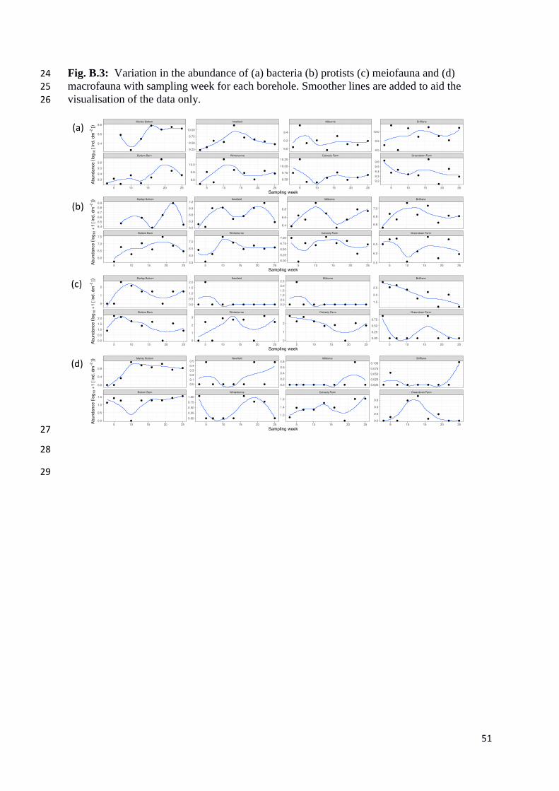
addition of borehole depth as an explanatory variable. Although bacteria and protists

increased in abundance over time in most boreholes (Fig. B.3), there was considerable

difference between boreholes regarding abundance peaks and (as a consequence) the

19

abundance patterns were unrelated to borehole depth (Table B.3) or any other variables we

investigated. Bacterial counts exceeded 109 ind. dm-2 and protists showed an average

abundance of ~70,000 ind. dm-2. While bacteria and protists were present in all boreholes and

on all sampling occasions, meiofauna and macrofauna were sometimes absent on particular

sampling occasions (Fig. B.3).

Meiofauna were always present in BB, BL, CF and MB and macrofauna were always

present in BB, CF and MB. In two of the boreholes, Bottom Barn and Calversley Farm,

macrofaunal abundance increased steadily from under 10 to over 40 individuals per dm2

(mainly N. kochianus and P. cavaticus) over the 25 weeks (Fig. B.3). Mean abundance of

meiofauna and macrofauna in the boreholes was ~ 5 ind. dm-2 and ~ 7 ind. dm-2 respectively.

We used mass-abundance spectra to estimate the response of the entire community.

As expected, over 10 orders of magnitude in body mass from bacteria to macrofauna (Figs. 3

and B.4), abundance declined linearly. The average slope of the size spectrum, across sites

and sampling occasions was -1.12 (95% CI: -1.16 to -1.07, Fig. 3). Size spectra slopes did not

vary systematically through time or with borehole depth (Table 3). However, a significant

time × depth interaction was evident (Table 3) with slopes becoming steeper (more negative)

through time for ‘shallower’ boreholes (Fig. 3). This pattern can be explained by the fact that,

whilst not individually significant, bacteria and protozoan abundances tended to increase

through time in the ‘shallower’ boreholes, whilst meiofauna and macrofauna abundances

were relatively constant (Fig. B.3). This is also supported by the marginally significant p-

value for the time × depth interaction for size spectra intercepts which were fixed at the

minimum body size class (Table 3).

20

4. Discussion

This study was the first to analyse the impacts of groundwater flooding induced

intensive recharge using an extensive analysis of both abiotic and biotic factors. We showed

that nutrient concentrations increased in response to elevated groundwater levels, with more

nutrients being available for groundwater organisms in consequence. Bacteria in the open

water (i.e. bacteria not associated with sediment) became more abundant as groundwater

levels and DOC concentrations decreased, indicating that they incorporated the additional

energy. The measures of bacterial functional richness show that bacterial richness was high

when DOC was high, demonstrating the link between nutrients and functional richness and

bacterial activity. This finding was further supported by the respiration study that revealed a

positive correlation between DOC concentrations and microbial metabolic activity in

boreholes (see 4.1 Open water chemistry and biota). In the sediment, the change over time

back to baseline levels was reflected in changes of the size distribution (measurements of

individual groups were less conclusive) of the community towards steeper M-N slopes

because, overall, small organisms (bacteria and protozoans) increased in abundance while the

larger ones did not. This was however not the case in the deeper aquifer which was also much

less affected by the flooding (see 4.2 Sediment biota).

4.1. Open water chemistry and biota

Groundwater that is enriched with nutrients (e.g. in catchments with intensive

agriculture) has previously been shown to exhibit high bacterial biodiversity values (Stein et

al., 2010), which is atypical for pristine groundwater of comparable systems (Griebler et al.,

2010). In accordance with these studies, we found that temporally variable DOC levels can

produce similar differences in bacterial richness over time (however, in our case measured as

functional richness not as operational taxonomic units used by these authors). Intriguingly,

21

the DOC pattern observed over time shows a ‘new pulse’ of nutrients after some weeks of

sampling. We can only speculate about the reasons behind this pattern but two scenarios are

possible: the new pulse could be the result of a new input from the surface or be the result of

food web responses: the pattern resembles nutrient dynamics in chemostats, where bacteria

can first utilise the nutrients, then crash and subsequently recover (e.g. Behrends et al., 2014).

4.2. Sediment biota

Intriguingly, with exception of the macrofauna in two of the boreholes, the sediment

biota (bacteria, protists, microscopic metazoans and macrofauna) did not show any

statistically significant response to the changes in nutrient concentrations or water table

(although trends of increasing abundance of bacteria and protists in the shallow aquifer were

obvious). The non-significance is largely due to two methodological issues: firstly, boreholes

were used as replicates, which ‘worked’ for very robust patterns such as water level decline,

DOC levels and size spectra, but for abundance patterns of individual groups each borehole

represents its own unique system (e.g. in some boreholes groups such as meiofauna were

almost absent despite the fact that the borehole connects to the same aquifer as a near-by

borehole with meiofauna; see Fig. B.3). Secondly, GAMM is a useful method to show trends

but it is not possible to fit linear correlations (such as fitting borehole depth as a predictor).

For all boreholes, species richness of macrofauna was similar to that reported

elsewhere in the UK (Robertson et al 2009) but lower than reported in Europe (Griebler et al.,

2010). Protozoan species richness was comparable to other studies outside the UK (Loquay et

al., 2009), possibly because protozoans can colonise ‘extreme’ habitats more easily than

metazoans. Previous studies on 5 of the 8 boreholes found the same macrofauna species, and

that, like this study, these species were more abundant than meiofaunal copepods (they

represent the majority of the meiofauna) (Johns et al., 2015; Maurice et al., 2016). This

22

pattern seems to be unique for groundwater habitats, for example, in streams, and rivers,

meiofauna are always more abundant than larger invertebrates (e.g. Stead et al. 2003) and

indeed, we would expect higher abundances of small invertebrates compared to larger ones

from metabolic theory (Brown et al., 2004).

We observed systematic changes in the size spectrum over the 25 weeks monitoring

period, with slopes of the size abundance relationship (the spectra) becoming steeper (more

negative) in the ‘shallower’ boreholes. This pattern is consistent with the notion that the

community dynamics at the bottom of shallower boreholes are more closely coupled with

conditions in the open water compared to deep boreholes. Shallow boreholes received

increased carbon resources and exhibited an increase in microbial biomass and metabolism

over the sampling period. In other words, compared to the shallow aquifer, the deeper aquifer

receives much less nutrients and water load when groundwater is flooded. These findings also

highlight that size spectra analysis can provide key insights into the responses of ecosystems

to environmental variability (Petchey and Belgrano, 2010) and understanding energy flow

through groundwater food webs.

The size spectra analysis also revealed that groundwater communities were strongly

size-structured with the slope of the relationships (N ~ M-1.1) similar to the negatively

isometric pattern often reported for aquatic food webs (Kerr and Dickie, 2001). For any given

size spectrum, the slope depends on the community-wide mean predator–prey mass ratio

(PPMR: the mean size of predators relative to prey), and the trophic transfer efficiency (TE:

the proportion of prey production converted to predator production) (Kerr and Dickie, 2001).

The model of Brown and Gillooly (2003) incorporates general allometric scaling principles to

predict the scaling of abundance, N, with body mass, M, as:

N ∝ Mλ × Mlog(TE)/log(PPMR), where λ is the M-N scaling coefficient within

trophic levels (typically −3/4), the reciprocal of the mass dependence of metabolic rate for

23

many multicellular taxa (Brown et al., 2004). The trophic structure of groundwater food webs

is largely unknown but assuming a TE range of between 10 and 20% (Jennings and

Mackinson, 2003) suggests that the PPMR ratio in these systems is somewhere between

100:1 and 600:1, similar to other benthic freshwater ecosystems (Perkins et al.2018,

Woodward and Warren 2007).

Abundances were generally high compared with other aquifer studies (Griebler et al.,

2010), which is explained by the fact that we sampled boreholes (Hahn and Matzke, 2005;

Sorensen et al., 2013) and did not pump the aquifer water (see references in Griebler and

Lueders, 2009 and Korbel et al., 2017). Collecting groundwater from boreholes is the most

common method for groundwater sampling because they provide the only suitable sampling

‘window’ into deeper aquifers. Previous studies have shown that boreholes have higher

abundance but the same species composition compared to the rest of the aquifer (Hahn and

Matzke, 2005, Sorensen et al., 2013). However, boreholes do still represent groundwater

community patterns over time (our focus) and species composition in the aquifer.

4.3. The wider context and future directions

Ecological assessment of groundwater is a very recent discipline (see reviews by

Danielopol et al., 2003; Gregory et al., 2014; Griebler et al., 2014; Steube et al., 2009).

However, we now have methods, such as cytometry (Bayer et al., 2016), that help us to

monitor stygobite populations and also to assess microscopically small organisms in

groundwater (see literature for bacteria, protists and meiofauna reviewed in Griebler and

Lueders (2009) and Novarino et al. (1997) for protists).

It will be crucial to determine if groundwater biota have the potential to buffer inputs

of nutrients through increased secondary production. Although their environment is stable,

the relatively low temperatures might inhibit the incorporation of these additional nutrients

24

into biomass. We believe a more rigorous analysis of the groundwater food web is needed to

show how the composition and activity of bacteria changes when nutrient availability

changes and whether the bacterial response is coupled with increased secondary production

of eukaryotes. Further, it is vital to include hydrological knowledge in these studies because

they determine how stable the habitat is. Menció et al. (2014) found that steadier groundwater

head levels and lower nitrate concentrations promote a more diverse and abundant stygofauna

community. Historical hydrological data from UK chalk aquifers, and our study, showed that

that the deep aquifer is less affected by flooding and it could therefore represent a very stable

environment for groundwater organisms. However, shallower aquifers (down to 100 m) seem

to respond rapidly to flooding and we do not know to what extent the groundwater

community is perturbed in these important underground layers that hold clean fresh water. As

extreme rainfall events are predicted to become more frequent in the Northern hemisphere, it

is likely that groundwater quality will ultimately be affected.

25

Acknowledgements

This study was funded by a NERC Urgency Grant NE/M005151/1. We would like to thank

the Environment Agency (Tim Jones) for supplying historical data for boreholes in the

aquifer we sampled. We would also like to acknowledge funding of PR for conducting the

smart tracer analysis through the INTERFACES FP7-PEOPLE-2013-ITN. We thank an

anonymous reviewer whose comments greatly improved this manuscript.

26

References

Armitage, P.D., Moss, D., Wright, J.F., Furse, M.T., 1983. The performance of a new

biological water quality score system based on macroinvertebrates over a wide range of

unpolluted running-water sites. Water Res. 17, 333–347.

Baho, D.L., Peter, H., Tranvik, L.J., 2012. Resistance and resilience of microbial

communities–temporal and spatial insurance against perturbations. Environ. Microbiol.

14, 2283–2292.

Bayer, A., Drexel, R., Weber, N., Griebler, C., 2016. Quantification of aquatic sediment

prokaryotes-A multiple-steps optimization testing sands from pristine and contaminated

aquifers. Limnologica 56, 6–13. https://doi.org/10.1016/j.limno.2015.11.003

Behrends, V., Maharjan, R.P., Ryall, B., Feng, L., Liu, B., Wang, L., Bundy, J.G., Ferenci,

T., 2014. A metabolic trade-off between phosphate and glucose utilization in

Escherichia coli. Mol. Biosyst. 10, 2820–2822. https://doi.org/10.1039/c4mb00313f

Boano, F., Harvey, J.W., Marion, A., Packman, A.I., Revelli, R., Ridolfi, L., Wörman, A.,

2014. Hyporheic flow and transport processes: Mechanisms, models, and

biogeochemical implications. Rev. Geophys. 52, 603–679.

Boulton, A.J., Findlay, S., Marmonier, P., Stanley, E.H., Valett, H.M., 1998. The functional

significance of the hyporheic zone in streams and rivers. Annu. Rev. Ecol. Syst. 29, 59–

81.

Boulton, A.J., Hancock, P.J., 2006. Rivers as groundwater-dependent ecosystems: a review of

degrees of dependency, riverine processes and management implications. Aust. J. Bot.

54, 133–144.

Brown, J., Gillooly, J., Allen, A., Savage, V., West, G., 2004. Toward a metabolic theory of

ecology. Ecology 85, 1771–1789.

Brown, J.H., Gillooly, J.F., 2003. Ecological food webs: high-quality data facilitate

theoretical unification. Proc. Natl. Acad. Sci. 100, 1467–1468.

Brunke, M., Gonser, T.O.M., 1997. The ecological significance of exchange processes

between rivers and groundwater. Freshw. Biol. 37, 1–33.

Christian, B.W., Lind, O.T., 2006. Key issues concerning Biolog use for aerobic and

anaerobic freshwater bacterial community-level physiological profiling. Int. Rev.

Hydrobiol. 91, 257–268. https://doi.org/10.1002/iroh.200510838

Danielopol, D.L., Griebler, C., Gunatilaka, A., Notenboom, J., 2003. Present state and future

prospects for groundwater ecosystems. Environ. Conserv. 30, 104–130.

Dossena, M., Yvon-Durocher, G., Grey, J., Montoya, J.M., Perkins, D.M., Trimmer, M.,

Woodward, G., 2012. Warming alters community size structure and ecosystem

functioning. Proc. R. Soc. London B Biol. Sci. 279, 3011–3019.

Ellis, B., Haaland, P., Hahne, F., Le Meur, N., Gopalakrishnan, N., Spidlen, J., Jiang, M.,

2009. flowCore: basic structures for flow cytometry data. R Packag. version 1.

Fuhrman, J.A., Azam, F., 1980. Bacterio Plankton Secondary Production Estimates for

27

Coastal Waters of British-Columbia Canada Antarctica and California Usa. Appl.

Environ. Microbiol. 39, 1085–1095.

Gasol, J.M., Del Giorgio, P.A., 2000. Using flow cytometry for counting natural planktonic

bacteria and understanding the structure of planktonic bacterial communities. Sci. Mar.

64, 197–224.

Gibert, J., Culver, D.C., Dole-Olivier, M.J., Malard, F., Christman, M.C., Deharveng, L.,

2009. Assessing and conserving groundwater biodiversity: Synthesis and perspectives.

Freshw. Biol. https://doi.org/10.1111/j.1365-2427.2009.02201.x

Gibert, J., Deharveng, L., 2002. Subterranean Ecosystems: A Truncated Functional

Biodiversity: This article emphasizes the truncated nature of subterranean biodiversity at

both the bottom (no primary producers) and the top (very few strict predators) of food

webs and discusses the implic. AIBS Bull. 52, 473–481.

Gregory, S.P., Maurice, L.D., West, J.M., Gooddy, D.C., 2014. Microbial communities in

UK aquifers: current understanding and future research needs. Q. J. Eng. Geol.

Hydrogeol. 47, 145–157.

Griebler, C., Avramov, M., 2014. Groundwater ecosystem services: a review. Freshw. Sci.

34, 355–367.

Griebler, C., Lueders, T., 2009. Microbial biodiversity in groundwater ecosystems. Freshw.

Biol. https://doi.org/10.1111/j.1365-2427.2008.02013.x

Griebler, C., Malard, F., Lefébure, T., 2014. Current developments in groundwater ecology—

from biodiversity to ecosystem function and services. Curr. Opin. Biotechnol. 27, 159–

167.

Griebler, C., Stein, H., Kellermann, C., Berkhoff, S., Brielmann, H., Schmidt, S., Selesi, D.,

Steube, C., Fuchs, A., Hahn, H.J., 2010. Ecological assessment of groundwater

ecosystems - Vision or illusion? Ecol. Eng. 36, 1174–1190.

https://doi.org/10.1016/j.ecoleng.2010.01.010

Haggerty, R., Martí, E., Argerich, A., Von Schiller, D., Grimm, N.B., 2009. Resazurin as a

“smart” tracer for quantifying metabolically active transient storage in stream

ecosystems. J. Geophys. Res. Biogeosciences 114.

Hahn, H.J., Matzke, D., 2005. A comparison of stygofauna communities inside and outside

groundwater bores. Limnol. Manag. Inl. Waters 35, 31–44.

Jennings, S., Mackinson, S., 2003. Abundance–body mass relationships in size‐structured

food webs. Ecol. Lett. 6, 971–974.

Johns, T., Jones, J.I., Knight, L., Maurice, L., Wood, P., Robertson, A., 2015. Regional-scale

drivers of groundwater faunal distributions. Freshw. Sci. 34, 316–328.

https://doi.org/10.1086/678460

Kerr, S.R., Dickie, L.M., 2001. The biomass spectrum: a predator-prey theory of aquatic

production. Columbia University Press.

Korbel, K.L., Hancock, P.J., Serov, P., Lim, R.P., Hose, G.C., 2013. Groundwater

ecosystems vary with land use across a mixed agricultural landscape. J. Environ. Qual.

28

42, 380–390.

Korbel, K., Chariton, A., Stephenson, S., Greenfield, P. and Hose, G.C., 2017. Wells provide

a distorted view of life in the aquifer: implications for sampling, monitoring and

assessment of groundwater ecosystems. Scientific Reports 7, 40702.

Krause, S., Hannah, D.M., Fleckenstein, J.H., Heppell, C.M., Kaeser, D., Pickup, R., Pinay,

G., Robertson, A.L., Wood, P.J., 2011. Inter‐disciplinary perspectives on processes in

the hyporheic zone. Ecohydrology 4, 481–499.

Krause, S., Lewandowski, J., Grimm, N.B., Hannah, D.M., Pinay, G., McDonald, K., Martí,

E., Argerich, A., Pfister, L., Klaus, J., 2017. Ecohydrological interfaces as hot spots of

ecosystem processes. Water Resour. Res. 53, 6359–6376.

Layer, K., Hildrew, A.G., Jenkins, G.B., Riede, J.O., Rossiter, S.J., Townsend, C.R.,

Woodward, G., 2011. Long-Term Dynamics of a Well-Characterised Food Web. Four

Decades of Acidification and Recovery in the Broadstone Stream Model System,

Advances in Ecological Research. https://doi.org/10.1016/B978-0-12-374794-5.00002-

X

Loquay, N., Wylezich, C., Arndt, H., 2009. Composition of groundwater nanoprotist

communities in different aquifers based on aliquot cultivation and genotype assessment

of cercomonads. Fundam. Appl. Limnol. 174, 261–269. https://doi.org/10.1127/1863-

9135/2009/0174-0261

Marmonier, P., Vervier, P., Giber, J., Dole-Olivier, M.-J., 1993. Biodiversity in ground

waters. Trends Ecol. Evol. 8, 392–395.

Maurice, L., Robertson, A.L., White, D., Knight, L., Johns, T., Edwards, F., Arietti, M.,

Sorensen, J.P.R., Weitowitz, D., Marchant, B.P., Bloomfield, J.P., 2016. The

invertebrate ecology of Chalk groundwaters. Hydrogeol. J. 24, 459–474.

McInerney, C.E., Maurice, L., Robertson, A.L., Knight, L.R.F.D., Arnscheidt, J., Venditti, C.,

Dooley, J.S.G., Mathers, T., Matthijs, S., Eriksson, K., 2014. The ancient Britons:

groundwater fauna survived extreme climate change over tens of millions of years

across NW Europe. Mol. Ecol. 23, 1153–1166.

Menció, A., Korbel, K.L., Hose, G.C., 2014. River-aquifer interactions and their relationship

to stygofauna assemblages: A case study of the Gwydir River alluvial aquifer (New

South Wales, Australia). Sci. Total Environ. 479–480, 292–305.

https://doi.org/10.1016/j.scitotenv.2014.02.009

Min, S.-K., Zhang, X., Zwiers, F.W., Hegerl, G.C., 2011. Human contribution to more-

intense precipitation extremes. Nature 470, 378–381.

Mulder, C., Elser, J.J., 2009. Soil acidity, ecological stoichiometry and allometric scaling in

grassland food webs. Glob. Chang. Biol. 15, 2730–2738. https://doi.org/10.1111/j.1365-

2486.2009.01899.x

Munro, A., Kovats, R.S., Rubin, G.J., Waite, T.D., Bone, A., Armstrong, B., Beck, C.R.,

Amlôt, R., Leonardi, G., Oliver, I., 2017. Effect of evacuation and displacement on the

association between flooding and mental health outcomes: a cross-sectional analysis of

UK survey data. Lancet Planet. Heal. 1, e134–e141.

29

Norland, S., Heldal, M., Tumyr, O., 1987. On the relation between dry matter and volume of

bacteria. Microb. Ecol. 13, 95–101. https://doi.org/10.1007/BF02011246

Novarino, G., Warren, A., Butler, H., Lambourne, G., Boxshall, A., Bateman, J., Kinner,

N.E., Harvey, R.W., Mosse, R.A., Teltsch, B., 1997. Protistan communities in aquifers:

A review, in: FEMS Microbiology Reviews. pp. 261–275.

https://doi.org/10.1016/S0168-6445(97)00046-6

O’Gorman, E.J., Pichler, D.E., Adams, G., Benstead, J.P., Cohen, H., Craig, N., Cross, W.F.,

Demars, B.O.L., Friberg, N., Gislason, G.M., 2012. Impacts of warming on the structure

and functioning of aquatic communities: individual-to ecosystem-level responses, in:

Advances in Ecological Research. Elsevier, pp. 81–176.

Perkins, D.M., Durance, I., Edwards, F.K., Grey, J., Hildrew, A.G., Jackson, M., Jones, J.I.,

Lauridsen, R., Layer-Dobra, K., Thompson, M., Woodward, G., 2018. Bending the

rules: exploitation of allochthonous resources by a top-predator modifies size abundance

scaling in stream food webs. Ecol. Lett. https://doi.org/10.1111/ele.13147.

Petchey, O.L., Belgrano, A., 2010. Body-size distributions and size-spectra: universal

indicators of ecological status?

R Development Core Team, 2017. A language and environment for statistical computing.

Reiss, J., Schmid-Araya, J.M., 2010. Life history allometries and production of small fauna.

Ecology 91, 497–507. https://doi.org/10.1890/08-1248.1

Reiss, J., Schmid-Araya, J.M., 2008. Existing in plenty: Abundance, biomass and diversity of

ciliates and meiofauna in small streams. Freshw. Biol. 53, 652–668.

https://doi.org/10.1111/j.1365-2427.2007.01907.x

Reuman, D.C., Mulder, C., Raffaelli, D., Cohen, J.E., 2008. Three allometric relations of

population density to body mass: theoretical integration and empirical tests in 149 food

webs. Ecol. Lett. 11, 1216–28. https://doi.org/10.1111/j.1461-0248.2008.01236.x

Robertson, A.L., Smith, J.W.N., Johns, T., Proudlove, G.S., 2009. The distribution and

diversity of stygobites in Great Britain: an analysis to inform groundwater management.

Geological Society of London.

Roger, F., Bertilsson, S., Langenheder, S., Osman, O.A., Gamfeldt, L., 2016. Effects of

multiple dimensions of bacterial diversity on functioning, stability and

multifunctionality. Ecology 97, 2716–2728.

Sarkar, D., Le Meur, N., Gentleman, R., 2008. Using flowViz to visualize flow cytometry

data. Bioinformatics 24, 878–879.

Schaum, C.-E., Barton, S., Bestion, E., Buckling, A., Garcia-Carreras, B., Lopez, P., Lowe,

C., Pawar, S., Smirnoff, N., Trimmer, M., 2017. Adaptation of phytoplankton to a

decade of experimental warming linked to increased photosynthesis. Nat. Ecol. Evol. 1,

94.

Schmid, P.E., 2000. Relation Between Population Density and Body Size in Stream

Communities. Science (80-. ). 289, 1557–1560.

https://doi.org/10.1126/science.289.5484.1557

30

Sorensen, J.P.R., Maurice, L., Edwards, F.K., Lapworth, D.J., Read, D.S., Allen, D., Butcher,

A.S., Newbold, L.K., Townsend, B.R., Williams, P.J., 2013. Using boreholes as

windows into groundwater ecosystems. PLoS One 8, e70264.

Stead, T.K., Schmid‐Araya, J.M., Hildrew, A.G., 2003. All creatures great and small: patterns

in the stream benthos across a wide range of metazoan body size. Freshw. Biol. 48, 532–

547.

Stefanowicz, A, 2006. The Biolog Plates Technique as a tool in ecological studies of

microbial communities. Polish J. Environ. Stud. 15, 669–676.

https://doi.org/http://dx.doi.org/10.3390/s120303253

Stein, H., Kellermann, C., Schmidt, S.I., Brielmann, H., Steube, C., Berkhoff, S.E., Fuchs, A.,

Hahn, H.J., Thulin, B., Griebler, C., 2010. The potential use of fauna and bacteria as

ecological indicators for the assessment of groundwater quality. J. Environ. Monit. 12,

242–254.

Steube, C., Richter, S., Griebler, C., 2009. First attempts towards an integrative concept for

the ecological assessment of groundwater ecosystems. Hydrogeol. J. 17, 23–35.

Taylor, R.G., Scanlon, B., Döll, P., Rodell, M., Van Beek, R., Wada, Y., Longuevergne, L.,

Leblanc, M., Famiglietti, J.S., Edmunds, M., 2013. Ground water and climate change.

Nat. Clim. Chang. 3, 322–329.

Taylor, R.G., Scanlon, B., Döll, P., Rodell, M., van Beek, R., Wada, Y., Longuevergne, L.,

Leblanc, M., Famiglietti, J.S., Edmunds, M., Konikow, L., Green, T.R., Chen, J.,

Taniguchi, M., Bierkens, M.F.P., MacDonald, A., Fan, Y., Maxwell, R.M., Yechieli, Y.,

Gurdak, J.J., Allen, D.M., Shamsudduha, M., Hiscock, K., Yeh, P.J.-F., Holman, I.,

Treidel, H., 2012. Ground water and climate change. Nat. Clim. Chang. 3, 322–329.

https://doi.org/10.1038/nclimate1744

Van Halem, D., Bakker, S.A., Amy, G.L., Van Dijk, J.C., 2009. Arsenic in drinking water: a

worldwide water quality concern for water supply companies. Drink. Water Eng. Sci. 2,

2009.

Weitowitz D., Maurice L., Lewis M., Bloomfield J., Reiss J. Robertson A.L., 2017. Defining

geo-habitats for groundwater ecosystem assessments: An example from England and

Wales (UK). Hydrogeology Journal. DOI:10.1007/s10040-017-1629-6

White, E.P., Ernest, S.K.M., Kerkhoff, A.J., Enquist, B.J., 2007. Relationships between body

size and abundance in ecology. Trends Ecol. Evol. 22, 323–30.

https://doi.org/10.1016/j.tree.2007.03.007

Woodward, G., Warren, P.H., 2007. Body size and predatory interactions in freshwaters:

scaling from individuals to communities. Body size Struct. Funct. Aquat. Ecosyst. 98–

117.

Yvon-Durocher, G., Reiss, J., Blanchard, J., Ebenman, B., Perkins, D.M., Reuman, D.C.,

Thierry, A., Woodward, G., Petchey, O.L., 2011a. Across ecosystem comparisons of

size structure: Methods, approaches and prospects. Oikos 120, 550–563.

https://doi.org/10.1111/j.1600-0706.2010.18863.x

Yvon-Durocher, G., Montoya, J.M., Trimmer, M., Woodward, G.U.Y., 2011b. Warming

31

alters the size spectrum and shifts the distribution of biomass in freshwater ecosystems.

Glob. Chang. Biol. 17, 1681–1694.

Zuur, A.F., Ieno, E.N., Walker, N.J., Saveliev, A.A., Smith, G.M., 2009. Mixed effects

models and extensions in ecology with R. Springer, New York.

32

Figure legends

Fig. 1: 10 yrs time series of the groundwater table (measured as metres below the surface) for

eight boreholes in the UK Chalk aquifer. The arrow shows the start of the flooding period

(induced by heavy rains in Winter 2013) and the area shaded in grey indicates the sampling

period (10 sampling occasions over 25 weeks). The water level on the y-axis is given as

mAOD (Metres Above Ordnance Datum); a value of zero indicates that the waterlevel had

reached the land surface.

33

Fig. 2: Water levels (a), DOC dynamics (b), bacterial biomass (c) and bacterial functional

richness (d) over a 25 weeks study period following the tail of groundwater flooding in a

chalk aquifer (two locations [Berkshire and Dorset] and a total of 8 boreholes). The plots are

the results of GLMM and the patterns over time are significant in all cases. Note that peaks

and dips in DOC correspond to those observed for dissolved organic carbon and functional

richness of bacteria.

34

Fig. 3: Upper panel: Body mass and abundance scaling in groundwater communities. The

average slope of the size spectrum, estimated from mixed-effects modelling, was - 1.12 (95%

CI: -1.16 to -1.07) across boreholes and sampling occasions. Lower panel: Variation in size

spectrum slopes in relation to sampling occasion and total borehole depth (here represented

by shading of data points). The size spectrum slope steepened with each sampling occasion in

the shallow boreholes (light grey data points).

35

Table 1

Overview of the biota found in eight boreholes showing sampling effort, body mass, number

of individuals measured and the total of functional groups/taxa recorded.

Group Total no

of

samples

scanned

Min DWC in

g

Max

DWC in

g

Total no of

individuals

measured

and

identified

Total functional

groups/taxa

Open water bacteria 80 0.0000000001 0.000001 >4Mio 31 functional groups

Sediment bacteria 77 0.0000000001 0.000001 >4Mio na

Protists 69 0.0000000428 0.000052 >2000 67

Meiofauna 77 0.0000321386 0.008484 >700 7

Macrofauna 77 0.0000681359 6.395189 >3000 9

Note: Across boreholes, this sampling resulted in 77 samples for open water bacteria (see

S1), 69 sediment samples for protists, 77 samples for meiofauna and macrofauna (see S1);

and 90 cotton strips were evaluated for fungal biomass (no ergosterol, i.e. fungal biomass,

was detected). DWC= dry weight carbon.

36

Table 2

Summary output from generalised additive mixed modelling (GAMM) of open water

parameters through time (sampling week).

Response Smoother term edf F p-value

Waterlevel s(time, k = 6) 4.14 3.83 0.007

DOC (log10) s(time, k = 6) 1.93 10.22 <.0001

Bacteria biomass (log10) s(time, k = 6) 3.85 5.51 <.0001

Functional diversity s(time, k = 6) 4.95 40.75 <.0001

Note: The results provide support for nonlinear temporal trends in response to flooding.

Significant terms are highlighted in bold, k refers to the number of knots in the smoother

term.

37

Table 3

Summary output from generalised least squares modelling (GLS) of size spectra parameters.

Size-spectrum slope

Size-spectrum

intercept

Term DF F-value p-value F-value p-value

Time 1,66 0.25 0.619 0.95 0.334

Depth 1,66 0 0.979 0.35 0.557

Time:Depth 1,66 4.98 0.029 2.89 0.094

Note: Significant terms are highlighted in bold.

38

APPENDIX A: APPENDICES TO THE METHODS

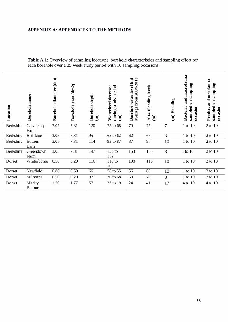
Table A.1: Overview of sampling locations, borehole characteristics and sampling effort for

each borehole over a 25 week study period with 10 sampling occasions.

Lo

cati

on

Bo

reh

ole

nam

e

Bo

reh

ole

dia

met

er (

dm

)

Bo

reh

ole

are

a (

dm

2)

Bo

reh

ole

dep

th

(m)

Wa

terl

evel

dec

rea

se

du

rin

g s

tud

y p

erio

d

(m)

Ba

seli

ne

wate

r le

vel

(m

)

av

era

ge

fro

m 2

00

4-2

01

3

20

14

Flo

od

ing

lev

els

(m)

(m)

Flo

od

ing

Ba

cter

ia a

nd

macr

ofa

un

a

sam

ple

d o

n s

am

pli

ng

occ

asi

on

Pro

tist

s a

nd

mei

ofa

un

a

sam

ple

d o

n s

am

pli

ng

occ

asi

on

Berkshire Calversley

Farm 3.05 7.31 120 75 to 68 70 75 7 1 to 10 2 to 10

Berkshire Brifflane 3.05 7.31 95 65 to 62 62 65 3 1 to 10 2 to 10

Berkshire Bottom

Barn

3.05 7.31 114 93 to 87 87 97 10 1 to 10 2 to 10

Berkshire Greendown

Farm

3.05 7.31 197 155 to

152

153 155 3 1to 10 2 to 10

Dorset Winterborne 0.50 0.20 116 113 to

103

108 116 10 1 to 10 2 to 10

Dorset Newfield 0.80 0.50 66 58 to 55 56 66 10 1 to 10 2 to 10

Dorset Milborne 0.50 0.20 87 70 to 68 68 76 8 1 to 10 2 to 10

Dorset Marley

Bottom

1.50 1.77 57 27 to 19 24 41 17 4 to 10 4 to 10

39

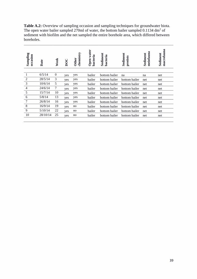
Table A.2: Overview of sampling occasion and sampling techniques for groundwater biota.

The open water bailer sampled 270ml of water, the bottom bailer sampled 0.1134 dm2 of

sediment with biofilm and the net sampled the entire borehole area, which differed between

boreholes.

Sa

mp

lin

g

occ

asi

on

Da

te

Wee

k

DO

C

Oth

er

chem

istr

y

Op

en w

ate

r

ba

cter

ia

Sed

imen

t

ba

cter

ia

Sed

imen

t

pro

tist

s

Sed

imen

t

mei

ofa

un

a

Sed

imen

t

ma

cro

fau

na

1 6/5/14 0 yes yes bailer bottom bailer na na net

2 28/5/14 3 yes yes bailer bottom bailer bottom bailer net net

3 10/6/14 5 yes yes bailer bottom bailer bottom bailer net net

4 24/6/14 7 yes yes bailer bottom bailer bottom bailer net net

5 15/7/14 10 yes yes bailer bottom bailer bottom bailer net net

6 5/8/14 13 yes yes bailer bottom bailer bottom bailer net net

7 26/8/14 16 yes yes bailer bottom bailer bottom bailer net net

8 16/9/14 19 yes no bailer bottom bailer bottom bailer net net

9 5/10/14 22 yes no bailer bottom bailer bottom bailer net net

10 28/10/14 25 yes no bailer bottom bailer bottom bailer net net

40

Table A.3: Overview of some borehole parameters: borehole depth, average oxygen

saturation (in %, averaged for 10 sampling occasions for the top water layer, the medium

water layer and the bottom of the borehole) and average abundance of invertebrates

(macrofauna, meiofauna and protozoans).

Loca

tion

Bore

hole

nam

e

Bore

hole

dep

th

O2 t

op

O2 m

idd

le

O2 b

ott

om

Macr

o-

fau

na

Mei

o-

fau

na

Pro

tozo

a

Ber

ksh

ire

Bottom Barn 114 81 64 54 18 1 105049

Brifflane 95 8 6 11 5 94964

Calversley Farm 120 81 80 80 23 5 76183

Greendown Farm 197 94 89 85 2 45498

Dors

et

Marley Bottom 57 74 74 75 7 2 52376

Milborne 87 81 82 79 5 60312

Newfield 66 55 47 33 2 2 71422

Winterborne 116 94 93 92 8 10 73009

41

Additional methods

Fungi

Cotton strips were frozen and used for the determination of fungal biomass via the

ergosterol method (Gessner and Chauvet, 1993; Gonçalves et al., 2013). Because the

ergosterol extraction did not give a positive result for fungi for any of the 90 samples tested,

we do not report any results on fungi in the results section. It is possible that in these

boreholes, no fungal mycelia were established on the cotton strips. Other studies have found

fungi in groundwater when exposing autoclaved leaf litter (Chauvet et al., 2016).

Nutrients

On seven sampling occasions, we also measured dissolved organic nitrogen (DON), nitrate

(NO3-), chlorine (Cl), sodium (Na+), Potassium (K+), magnesium (Mg2+), calcium (Ca2+)

and sulphate (SO4 ). These data are not reported here.

Microbial Metabolic Activity

On the second sampling occasion only, we took samples to characterise the metabolic

activity in the boreholes (except for MB) and relate these measurements to DOC levels at that

time. Microbial metabolic activity and ecosystem respiration was measured by applying the

“smart tracer” Resazuring/Resorufin (Raz/Rru) system that has been first used in

ecohydrological applications by (Haggerty et al., 2008). It has since been applied in reach-

scale field experiments, flume-scale (Haggerty et al., 2014) and been introduced for

microcosm incubation studies by (Baranov et al., 2016). Raz, a weakly-fluorescent substance

transforms under mildly reducing conditions irreversibly to the highly-fluorescent Rru, thus,

42

representing an indicator of microbial metabolic activity and being correlated to aerobic

respiration (Haggerty et al., 2008).

Raz to Rru conversion was measured in this study by fluorometry using excitation and

emission wavelengths of 570 nm and 585 nm, respectively. Therefore, groundwater samples

collected between 28 May 2014 and 30 May 2014 were cooled and transferred to the

laboratory without filtering to preserve the microbial community that could be present. For

incubations, 250 ml of sampled groundwater was incubated in 1000 ml microcosms with a

concentration of 100 µg/l Raz for 24 hrs. Each sample was incubated in duplicate. Two

microcosms were prepared with only deionised water to act as control treatments. Incubations

started on 9 June 2014.

The Raz to Rru conversion ratio was quantified at t=0, 2, 4, 6, 8 and 24 hours of

incubation by measuring both compounds for filtered samples using Albilla GGUN-FL 30

(Albillia, Neuchatel, CH) bench top fluorimeters (Baranov et al., 2016; Lemke et al., 2013).

Samples were discarded after measurement. Microcosms were incubated in an incubation

fridge, shielded from light, at 12±0.12°C. Temperature was monitored using a Tinytag

Aquatic 2 temperature logger (Gemini Data Loggers Ltd, Chichester, United Kingdom). The

raz-to-rru conversion rate was calculated as:

𝑟𝑒𝑠𝑝𝑖𝑟𝑎𝑡𝑖𝑜𝑛𝑡 = 𝑙𝑛(𝑟𝑟𝑢𝑡𝑟𝑎𝑧𝑡

+ 𝐶) Eq. 1

with C = 1, which is a constant value for amount of tracer recovered. Respiration at time t

was calculated for each time step, through which a simple linear regression line was fitted.

The slope of this line was then compared between all samples, where a higher value

correlates with higher microbial metabolic activity.

References

Baranov, V., Lewandowski, J., Krause, S., 2016. Bioturbation enhances the aerobic

43

respiration of lake sediments in warming lakes. Biol. Lett. 12, 20160448.

Chauvet, E., Cornut, J., Sridhar, K.R., Selosse, M.-A., Bärlocher, F., 2016. Beyond the water

column: aquatic hyphomycetes outside their preferred habitat. Fungal Ecol. 19, 112–

127.

Gessner, M.O., Chauvet, E., 1993. Ergosterol-to-biomass conversion factors for aquatic

hyphomycetes. Appl. Environ. Microbiol. 59, 502–507.

Gonçalves, A.L., Graça, M.A.S., Canhoto, C., 2013. The effect of temperature on leaf

decomposition and diversity of associated aquatic hyphomycetes depends on the

substrate. Fungal Ecol. 6, 546–553.

Haggerty, R., Argerich, A., Martí, E., 2008. Development of a “smart” tracer for the

assessment of microbiological activity and sediment-water interaction in natural waters:

The resazurin-resorufin system. Water Resour. Res. 44, 1–10.

https://doi.org/10.1029/2007WR006670

Haggerty, R., Ribot, M., Singer, G.A., Martí, E., Argerich, A., Agell, G., Battin, T.J., 2014.

Ecosystem respiration increases with biofilm growth and bed forms: Flume

measurements with resazurin. J. Geophys. Res. Biogeosciences 119, 2220–2230.

Lemke, D., Liao, Z., Wöhling, T., Osenbrück, K., Cirpka, O.A., 2013. Concurrent

conservative and reactive tracer tests in a stream undergoing hyporheic exchange. Water

Resour. Res. 49, 3024–3037.

44

Fig. A.1: Cell size calibration from flow cytometry data. Cell size (μm) was estimated from

the relationship between calibration beads of known size and forward scatter values returned

by flow cytometer.

45

APPENDIX B: APPENDICES TO THE RESULTS

Table B.1: Output of GAMM modelling testing for the significance of the temporal

autocorrelation term. The significance of the temporal autocorrelation term was determined

by comparing nested models with (Mcor) and without the autocorrelation term (M) via a

likelihood ratio test. The value ρ is generally high and indicates that residuals separated by

one week have a correlation of >0.70.

Response Term ρ F p-value

Waterlevel Anova (Mcor, M) 1.00 425.51 <.0001

DOC (log10) Anova (Mcor, M) 0.74 51.62 <.0001

Bacteria biomass (log10) Anova (Mcor, M) 0.95 1451.06 <.0001

Functional diversity Anova (Mcor, M) 0.93 1282.06 <.0001

46

Table B.2: List of taxa found within the macrofauna, meiofauna and protozoans. The number

after the taxon name indicates its relative abundance within that group. The most frequent

and abundant taxa are in bold.

Protists continued

1 Crangonyx subterraneus 1.76 25 Holophrya sp. 0.04

2 Microniphargus leruthi 1.95 26 Holosticha sp. 1.27

3 Niphargus fontanus 0.72 27 Hymenostomata 0.04

4 Niphargus glenniei 0.03 28 Hypotrich 0.63

5 Niphargus kochianus 91.43 29 Kahlilembus attenuatus 0.08

6 Niphargus spec. 2.23 30 Lacrymaria sp. 0.21

7 Planaria 0.03 31 Linostoma vorticella 0.08

8 Proasellus cavaticus 1.82 32 Litonotus sp. 0.85

9 Turbellarian 0.03 33 Loxodes sp. 0.04

34 Metopus sp. 0.08

35 Nassula sp. 0.08

1 Copepoda 94.25 36 Oligotrich ciliate 0.17

2 Nematoda 2.24 37 Oxytricha sp. 0.08

3 Paracyclops 0.14 38 Parameciumsp. 3.10

4 Rotifera 0.70 39 Parapodophyra conf 0.04

5 Stenostomum sp. 0.70 40 Peritrich cilaite 0.04

6 Testudinella sp. 0.14 41 Phascolodon sp. 0.04

7 Turbellaria 0.42 42 Phialina sp. 0.89

43 Placus luciae 0.04

Protists 44 Protist species 0.04

1 Amoeba 0.04 45 Pseudochilodonopsis sp. 0.04

2 Amphileptus sp. 1.23 46 Pseudomicrothorax sp. 0.13

3 Arcella sp. 0.51 47 round flagellate 0.08

4 Aspidisca sp. 0.47 48 small ciliate 4.29

5 Astylozoon sp. 0.25 49 small ciliate noID 0.64

6 Bursaria sp. 0.34 50 small ciliatenoID 0.47

7 Chanea stricta 3.61 51 small ciliatenoIDBL1 1.36

8 Chilodonella sp. 1.19 52 small flagellate 0.42

9 Chilondontopsis depressa 0.04 53 small flagellate noID 0.13

10 Ciliate noID 1 0.08 54 Strombidium sp. 0.42

11 Ciliate noID 2 0.13 55 Stylonychia sp. 0.04

12 Colpoda sp. 0.89 56 Suctoria swarmer 1.23

13 Enchelymorpha vermicularis 0.08 57 Tachysoma sp. 0.72

14 Euglena sp. 0.25 58 Tetrahymena sp. 1.36

15 Euglypha sp. 0.04 59 thecamoeba 0.21

16 Euplotes sp. 0.04 60 Thigmogaster sp. 0.04

17 Euplotes moebiusi 0.04 61 tiny ciliate 23.02

18 Flagellata 0.38 62 tiny flagellate 27.49

19 Flagellate colony 0.08 63 Trochilia sp. 1.61

20 Frontonia sp. 0.08 64 Uronema sp. 0.17

21 Glaucoma sp. 0.42 65 Urotricha sp. 1.06

22 Glaucoma scintillans 1.87 66 Vampyrella sp. 14.66

23 Gymnostom 0.04 67 Vorticella sp. 0.13

24 Heliozoan 0.21

Macrofauna

Metazoan meiofauna

47

Table B.3: Statistics for sediment biota and time. Summary output from generalised least

squares modelling (GLS) of organism groups sampled from sediments.

Bacteria Protists Meiofauna Macrofauna

Term

D

F

F-

value

p-

valu

e

D

F

F-

value

p-

valu

e

D

F

F-

value

p-

valu

e

D

F

F-

value

p-

valu

e

Time

1,6

6 0.46

0.50

1

1,6

4 1.91

0.17

2

1,6

8 0.37

0.54

7

1,6

8 0.43

0.51

5

Depth

1,6

6 0.11

0.74

5

1,6

4 2.89

0.09

4

1,6

8 0.06

0.80

5

1,6

8 0.01

0.91

2

Time:D

epth

1,6

6 0.71

0.40

2

1,6

4 1.16

0.28

6

1,6

8 0.04

0.83

8

1,6

8 0.40

0.53

1

48

1

2 Table B.4: Statistics for sediment biota and time. Summary output from generalised additive 3 mixed modelling (GAMM) of abundances of organism groups sampled from borehole 4 sediments through time (sampling week). No significant patterns were evident highlighting 5

system specific responses to recovery from ground water flooding. k refers to the number of 6 knots in the smoother term. 7

8

9

Response Smoother term edf F p-value

Bacteria s(time, k = 6) 1.00 0.46 0.500

Protists s(time, k = 6) 1.00 1.85 0.178

Meiofauna s(time, k = 6) 1.00 0.50 0.48

Macrofauna s(time, k = 6) 1.00 0.51 0.477

10

11

12

49

Fig. B.1: Variation in (a) waterlevel (b) DOC (c) bacterial biomass and (d) bacterial 13

functional richness with sampling week for each borehole. Smoother lines are added to aid 14

the visualisation of the data only. 15

16

17

50

Fig. B.2: Relationship between DOC and microbial metabolic activity (top) and between 18

nitrate and microbial metabolic activity (bottom) for all analysed boreholes 19

20

21

22

23

51

Fig. B.3: Variation in the abundance of (a) bacteria (b) protists (c) meiofauna and (d) 24

macrofauna with sampling week for each borehole. Smoother lines are added to aid the 25

visualisation of the data only. 26

27

28

29

52

Figure B.4: Body mass - abundance (M-N) relationships constructed for each borehole and 30

sampling occasion. Each data points represent the total abundance of organisms within that 31

(logarithmic) body mass class. 32

33

34

●● ●

●●●

●●●● ●

● ●●

●●

●●

●

● ●●

●

●● ●

●●

●●

●

●●

●●

●

●●

●

●●

●

●

●

●● ●

●●

●

●

●●●●

●

●●

●●

●

● ●●

●●

●

●

● ●●

●●

●

●

●

●●

●

●

● ● ●

●

●●

●● ●

● ●

●●

●●

●

●

● ●

●●●●●●

●●●● ●

● ● ●●

●

● ●●

● ●●

●

●● ●

●

●●

●●

● ●●

●

●●

●

●●

●

●

●● ●

●●

● ●

●● ●

●●●

●●●● ●

●●

●●

● ●

●

●●

●●

●●

●●

●●

●

● ●●

●

●●

●

●

● ●●

●

●●

●●

●●

●

● ●●

● ●●●●●

●●●● ●

●●

●● ●

●●

●

●●

●

●

● ●

●●

●

●●

● ●●

●

● ●

●●

●

● ●

●

●●

●●

●

●●

●

●● ●

●●●

●●●

● ●

●●

●●

● ●

●

● ●●

●

● ● ●

●●

●

● ●

●

●●

●●

● ●

● ●●

●

●●

●●

●●

●

●●

●

●● ●

●●●

●

●●●● ●

●● ●

●●

●

● ●●

●

● ●

●●

●

●

●

● ●●

●

● ●

● ●●

●

● ●

● ● ●●

●

●●

●

●● ●

●●●

●●●● ●

●

●● ●

●

● ●

● ●●

●

● ● ●

●●

●

●

● ●

●

● ●●

●

● ● ●

●

● ●●

●

●●

●●

●

●●

●

● ● ●●●

●

●●●

●●

●●

●●

●

●●

● ●●

●

● ● ●

●●

●

●

●

● ●●

●

● ● ●

● ●●

●

3 5 7 10 13 16 19 22 25

Ma

rley B

otto

mN

ew

field

Milb

orn

eB

rifflan

eB

otto

m B

arn

Win

terb

orn

eC

alv

esly

Fa

rmG

ree

nd

ow

n F

arm

−10.0 −7.5 −5.0 −2.5 0.0−10.0 −7.5 −5.0 −2.5 0.0−10.0 −7.5 −5.0 −2.5 0.0−10.0 −7.5 −5.0 −2.5 0.0−10.0 −7.5 −5.0 −2.5 0.0−10.0 −7.5 −5.0 −2.5 0.0−10.0 −7.5 −5.0 −2.5 0.0−10.0 −7.5 −5.0 −2.5 0.0−10.0 −7.5 −5.0 −2.5 0.0

0

3

6

9

0.0

2.5

5.0

7.5

10.0

2.5

5.0

7.5

10.0

0

3

6

9

0.0

2.5

5.0

7.5

10.0

2.5

5.0

7.5

10.0

0.0

2.5

5.0

7.5

10.0

0.0

2.5

5.0

7.5

10.0

Body mass (log10 [ mg C ])

Abund

an

ce

(lo

g1

0 [

in

d. dm

-2 ])

53

Fig. B.5: Variation in (a) slope and (b) intercept of size spectra relationships with sampling 35

week for each borehole. Smoother lines are added to aid the visualisation of the data only. 36

37

38

39

40

41