Grating Assisted Coupling of Light BetweenSemiconductor and Glass Waveguides ∗

Jerome K. Butler, Nai-Hsiang Sun and Gary A. EvansSouthern Methodist University

Dallas, TX 75275Lily Pang and Phil Congdon

Texas Instruments, Inc.Dallas, TX 75243

February 28, 2003

Abstract

Floquet-Bloch theory is used to calculate the electromagnetic fields in a leaky-mode grating-assisted directional coupler (LM-GADC) fabricated with semiconductorand glass materials. One waveguide is made from semiconductor materials (refractiveindex ≈ 3.2) while the second is made from glass (refractive index ≈ 1.45). The cou-pling of light between the two waveguides is assisted by a grating fabricated at theinterface of the glass and semiconductor materials. Unlike typical GADC structureswhere power is exchanged between two waveguides using bound modes, this semi-conductor/glass combination couples power between two waveguides using a boundmode (confined to the semiconductor) and a leaky mode (associated with the glass).The characteristics of the LM-GADC are discussed. Such LM-GADC couplers areexpected to have numerous applications in areas such as laser-fiber coupling, photonicintegrated circuits, and on-chip optical clock distribution. Analyses indicate that sim-ple LM-GADCs can couple over 40 % of the optical power from one waveguide toanother in distances less than 1.25 mm.

∗This work was supported by DARPA under Contract DAAL01-95-C-3524

1

I. Introduction

The ability to couple diode laser outputs monolithically and efficiently to a low lossco-integrated glass optical waveguide will enable applications such as large scale photonicintegrated circuits, on chip optical clock distributions for high speed microprocessors, andcompact wavelength division multiplexing laser sources.

In this paper, we present a new architecture of an integrated grating-assisted directionalcoupler (GADC) which is made of a III-V waveguide (neff ≈ 3.2) and a phosphorus-dopedsilica glass (PSG) waveguide (neff ≈ 1.45). The use of glass waveguides offers the com-bination of very low loss (<0.01 dB/cm), silicon process compatibility, and simple, lowcost fabrication processes. In addition, the PSG waveguide can have mode fields that arenearly identical in shape to the fields of a single-mode fiber. The near perfect match ofproperly designed PSG waveguide optical fields with those of an optical fiber produces>95 % butt coupling between the PSG waveguide and a single mode optical fiber withoutexternal optics.

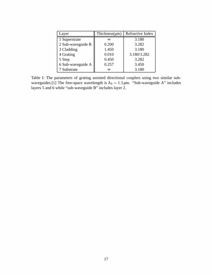
A GADC consisting of two non-synchronous waveguides and a separate grating regionis in reality a single, composite waveguide. However, for clarity, we will refer to two sub-waveguides called “sub-waveguide S (semiconductor)” and “sub-waveguide G (glass)”.In applications such as the one discussed in this paper the geometry of the two waveg-uides (waveguide dimensions as well as their corresponding refractive indices) are greatlydifferent. Assuming the two waveguides S and G are uncoupled and that each supportsonly a single mode, the modes of the two individual guides would have large differencesin their effective indices. To strongly couple the two waveguides, a grating is designedto phase-match the longitudinal propagation constants of the individual waveguides. InGADCs consisting of two guides with similar refractive indices but with different geomet-rical shapes, the effective indices of the individual modes are similar. In the latter case,the grating wavenumber, used to phase-match the longitudinal propagation constants of theindividual modes is rather small. Table I shows refractive indices and layer thicknesses ofsuch an extensively studied GADC structure [1]. Although the two coupled waveguides arenot identical, each supports a bound mode and each is composed of “similar” materials.

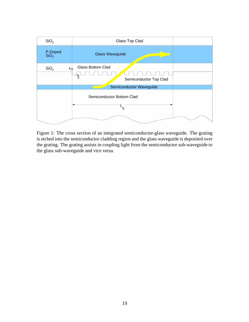
Figure 1 shows a cross section of a leaky-mode grating-assisted directional coupler(LM-GADC), which consists of a laser waveguide integrated with a PSG waveguide. Thecodirectional grating coupler, in the central region of the figure, has a grating layer oflength Lg. The rectangular-tooth grating layer is composed of semiconductor material inone region and glass in the other. Outside the grating region (z < 0 and z > Lg), the two sub-waveguides have negligible interaction, i.e., no significant power can be coupled from thesemiconductor sub-waveguide to the glass sub-waveguide and vice versa. In this study, theLM-GADC is excited with a laser mode, where the optical field is predominantly confinedto the semiconductor waveguide, at the LM-GADC input, z = 0. The coupling efficiencyis computed by calculating the percentage of power at the input that is coupled to the glasswaveguide at the output, z = Lg. In the region z > Lg, there will be no interaction betweenthe two sub-waveguides.

The analysis of the coupling between the glass and semiconductor layers is for a slabstructure. (The geometry has infinite extensions along the lateral y direction.) Accordingly,

2

the results obtained are reasonably accurate for a structure whose transverse mode width(x-direction) is small compared to the lateral mode width (y-direction).

The index profile of the semiconductor-glass LM-GADC is shown in Fig. 2. Unlike typ-ical GADCs, where the power exchange between the two sub-waveguides occurs via boundmodes, the semiconductor-glass LM-GADC exchanges power between sub-waveguides us-ing a bound mode of the semiconductor sub-waveguide and a (fundamental) leaky mode ofthe glass sub-waveguide. In Fig. 2 the index of refraction of the core in the glass region ismuch smaller than the index of refraction of the semiconductor substrate. This high indexmismatch causes the modes of the glass waveguide to leak energy to the semiconductorsubstrate. As a result, mode propagation in the glass waveguide attenuates due to powerloss to the semiconductor substrate.

The concept of the grating coupler causing the two lowest-order modes of the compositewaveguide to have similar power distributions in each sub-waveguide was developed in [2]for typical GADCs. This same concept and the resulting physical processes for powerexchange between the two sub-waveguides applies directly to LM-GADCs. However inthe latter device, the losses of each sub-waveguide can be large and unequal. As a resultof these large and unequal losses, the maximum power transfer between sub-waveguidesoccurs before the power in the other sub-waveguide is a minimum.

The most common, simple, and intuitive theoretical analyses of the GADC are basedon coupled-mode theory (CMT) which finds the coupling length, the coupled power dis-tribution, and the resonant grating period [1],[3] –[14]. Also, a transfer matrix method(TMM) approach using the mode-matching technique has been introduced to examine thepower coupling and radiation loss of the GADC structure [15]. To date, CMT or TMMapproaches have not been applied to GADC structures with interacting leaky modes or tostructures with layers that have material losses.

Rather than add corrections to the CMT or TMM approaches, we use the Floquet-Blochtheory [16]–[19] to analyze the LM-GADC problem because it accounts for radiation lossesfrom leaky modes as well as material losses in the various layers in a straightforward man-ner. In general, the Floquet-Bloch analysis calculates radiation losses of the LM-GADCfrom fundamental principles [2].

In Section II, a brief introduction of the Floquet-Bloch theory [17] is presented. Anexample of the typical GADC is discussed in Section III. Then, we analyze the LM-GADCstructure shown in Figs. 1 and 2. The complete field distributions and dispersion and atten-uation characteristics are discussed in Section IV. In Section V, the power coupling mech-anism of the semiconductor-glass LM-GADC is discussed.

II. Problem Formulation

Consider a dielectric waveguide with arbitrary layers including a periodic grating layer.The dielectric superstrate and substrate regions are assumed to be half spaces. The dielec-tric materials in each layer (except the grating layer) are isotropic and homogeneous. Awave with time variation of the form exp( jωt) is assumed to propagate in the z direction(see Fig. 1), as exp(−γz). The complex longitudinal propagation constant is γ = α + jβ.For the sake of simplicity assume the field is invariant with respect to y.

3

Characteristic Modes

For the GADC and LM-GADC structures, the field expressions which are written inFloquet-Bloch form must satisfy the boundary conditions at each interface. Assumingtransverse electric (TE) polarization, the y-component of the electric field in the i-th layer,

E(i)y , can be written as

E(i)y (x,y) = f (i)(x,z)e−γz

= e−(α+ jβ)z∞

∑n=−∞

f (i)n (x)e− jnKz =

∞

∑n=−∞

f (i)n (x)e− jkznz, (1)

where K = 2π/Λ is the grating wavenumber, Λ is the grating period, n is the space harmonic

order, i indicates the i-th layer, and f (i)n is the amplitude of the nth space harmonic. The

function f (i) is periodic and satisfies f (i)(x,z) = f (i)(x,z+Λ). The term kzn is the complexpropagation constant of the nth spatial harmonic and can be written as

kzn = (β+nK)− jα = βn − jα, (2)

where βn, the real part of kzn, is the longitudinal propagation constant of the n-th spaceharmonic, and α (> 0), the imaginary part of kzn, is the attenuation constant due to leakymodes as well as material losses. Similarly, the magnetic field along the z direction in the

ith layer, H(i)z can be expressed as

H(i)z =

∞

∑n=−∞

h(i)n e− jkznz, (3)

where h(i)n is the nth space harmonic component of the magnetic field in the ith layer.

Outside the grating layer, the scalar Helmholtz equation can be written as

d2 f (i)n (x)

dx2 +[k2εi− k2zn] f (i)

n (x) = 0, (4)

where k = 2π/λ is the free space wavenumber, εi is the relative dielectric constant of the ithlayer, and the complex transverse wavenumber for the nth space harmonic in the ith layer

is defined by (k(i)zn )2 = εik2

− k2zn.

The interesting features of Floquet-Bloch modes, including the generation of space har-monics results from the periodic grating layer. Because the refractive index in the gratinglayer is nonuniform and varies periodically along the propagation direction, the permittivitycan be expressed as a Fourier series

ε(x,z) = ∑n

εn(x)e jnKz. (5)

The field solution for TE modes in the grating layer is obtained by solving the equivalentMaxwell’s equations instead of (4):

d~f (g)

dx= Q(kz0·)~h

(g)(x), (6)

4

andd~h(g)

dx= P(kz0·)~f

(g)(x), (7)

where g stands for the grating layer, and the variable kz0 is the complex propagation con-stant of the 0-th spatial harmonic. The vectors ~f (g)(x) and~h(g)(x) are formed by the group

of spatial harmonics f (g)n (x) and h(g)

n (x), respectively, where f (g)n (x) and h(g)

n (x) are definedby (1) and (3). For TE polarization, the square matrices P(kz0) and Q(kz0) have elementsPnm = jωε0[(kzn/k)2δnm − εn−m] and Qnm = jωµ0δnm, respectively, where δnm is the Kro-necker delta.

The solutions of the Helmholtz equation (4) are given by the linear combination of

exp( jk(i)zn x) and exp(− jk(i)

zn x), while the equivalent Maxwell’s equations (6) and (7) can besolved by the fourth-order Runge-Kutta method [20]. A resulting characteristic equationis obtained by appropriately matching the boundary conditions and simultaneously solving(6) and (7). Considering transverse electric polarization, the field components and theirnormal derivatives must be continuous at each interface. After appropriate substitution, weobtain a system of linear equations D(kz0) · ~f (xk−1) = 0 with the unknown variable kz0,where D is a square matrix, and ~f (xk−1) is the initial value of the field at the bottom of thegrating layer. The system of linear equations has a nontrivial solution when[2]

det[D(kz0)] = 0. (8)

After solving for the roots of (8) numerically[20], the Floquet amplitudes of all space har-monics for the field distribution in all layers can be evaluated.

Kinematic Properties

Many of the modal interaction features of grating-assisted couplers can be understoodby analyzing the “ω−β” plot shown in Fig. 3. (The lines in the figure do not represent theactual dispersion curves of the modes or the space harmonics.) In the present case we willconsider two Floquet-Bloch modes of the LM-GADC, labeled mode A and mode B. Whenthe modes do not interact, say at some position below resonance (small Λ values), mode Arepresents the mode of the semiconductor waveguide, while mode B represents the modeof the glass waveguide. Away from resonance the field distribution of the modes will bealmost identical to the modes of the individual sub-waveguides in the absence of the other.Mode A has an effective index, nA, that lies between 3.386 and 3.165, while mode B hasan effective index, nB, lying between 1.458 and 1.448. The lower bound on nA is 3.165and the lower bound for nB is 1.448. In Fig. 3, the slope of the line representing mode Ais 1/3.165 and the slope of the line representing mode B is 1/1.448. The actual dispersioncurves will lie slightly below the two dark lines of the figure.

The space harmonics for the two modes intersect at an infinite number of positions,represented by the points Ii, j, where i represents the space harmonic of mode A and jrepresents the space harmonic of mode B. The two cone regions about the kΛ axis arethe superstrate fast-wave region (FWR) and substrate FWR. It should be noted that the

5

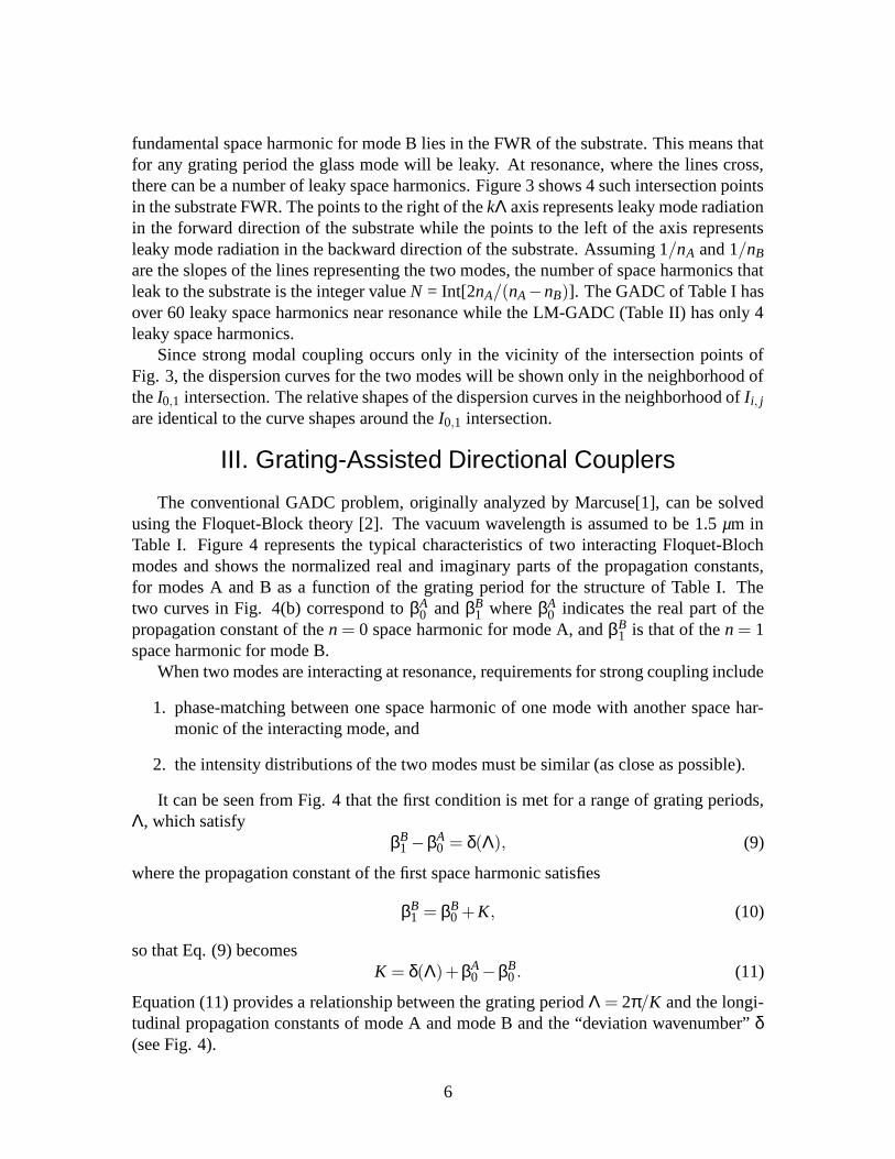
fundamental space harmonic for mode B lies in the FWR of the substrate. This means thatfor any grating period the glass mode will be leaky. At resonance, where the lines cross,there can be a number of leaky space harmonics. Figure 3 shows 4 such intersection pointsin the substrate FWR. The points to the right of the kΛ axis represents leaky mode radiationin the forward direction of the substrate while the points to the left of the axis representsleaky mode radiation in the backward direction of the substrate. Assuming 1/nA and 1/nB

are the slopes of the lines representing the two modes, the number of space harmonics thatleak to the substrate is the integer value N = Int[2nA/(nA−nB)]. The GADC of Table I hasover 60 leaky space harmonics near resonance while the LM-GADC (Table II) has only 4leaky space harmonics.

Since strong modal coupling occurs only in the vicinity of the intersection points ofFig. 3, the dispersion curves for the two modes will be shown only in the neighborhood ofthe I0,1 intersection. The relative shapes of the dispersion curves in the neighborhood of Ii, j

are identical to the curve shapes around the I0,1 intersection.

III. Grating-Assisted Directional Couplers

The conventional GADC problem, originally analyzed by Marcuse[1], can be solvedusing the Floquet-Block theory [2]. The vacuum wavelength is assumed to be 1.5 µm inTable I. Figure 4 represents the typical characteristics of two interacting Floquet-Blochmodes and shows the normalized real and imaginary parts of the propagation constants,for modes A and B as a function of the grating period for the structure of Table I. Thetwo curves in Fig. 4(b) correspond to βA

0 and βB1 where βA

0 indicates the real part of thepropagation constant of the n = 0 space harmonic for mode A, and βB

1 is that of the n = 1space harmonic for mode B.

When two modes are interacting at resonance, requirements for strong coupling include

1. phase-matching between one space harmonic of one mode with another space har-monic of the interacting mode, and

2. the intensity distributions of the two modes must be similar (as close as possible).

It can be seen from Fig. 4 that the first condition is met for a range of grating periods,Λ, which satisfy

βB1 −βA

0 = δ(Λ), (9)

where the propagation constant of the first space harmonic satisfies

βB1 = βB

0 +K, (10)

so that Eq. (9) becomesK = δ(Λ)+βA

0 −βB0 . (11)

Equation (11) provides a relationship between the grating period Λ = 2π/K and the longi-tudinal propagation constants of mode A and mode B and the “deviation wavenumber” δ(see Fig. 4).

6

Although Eq. (11) insures phase matching, it does not guarantee that a large fractionof power will be transferred between sub-waveguides. To insure significant power transferthe modes must have nearly identical power distributions (the second condition above).Modes A and B are closest to having identical intensity shapes when their longitudinalpropagation constants differ by approximately K, the grating wavenumber. This occurswhen δ is a minimum.

The normalized attenuation for the two modes for the structure of Table I is shownin Fig. 4. It should be noted that all space harmonics for each mode exhibit identicalattenuation. In the vicinity of resonance, the power losses are low and nearly identical forboth modes, ranging from about 8× 10−5/mm to 8.3× 10−4/mm. Since these losses arenegligible, the coupling length Lc can be estimated (with less than 2 % error) by [2]

Lc =πδ. (12)

The grating period Λ = 14.0387µm, corresponding to δmin/k ≈ 6.5× 10−4 produces acoupling length of about 11.5 mm or 7,700 grating periods for a grating depth of 0.01µm.This long coupling length occurs because of the very weak grating. Stronger gratingsproduce much shorter coupling lengths.[2] The grating period at the point when δ is aminimum differs only slightly from the grating period when αA = αB.

The propagation characteristics described in Fig. 4 illustrate the standard behavior fortypical GADC devices which exchange power between bound modes. A key point for theGADC is that the modal losses are negligible for the typical GADC so that the couplingefficiency approaches 100 percent, and the coupling length is given by Eq. (12).

IV. Leaky Mode Grating-Assisted Directional Couplers

Consider now the structure of the semiconductor/glass LM-GADC, as shown in Figs. 1and 2, with parameters given in Table II. In the leaky mode coupler, sub-waveguide S refersto the semiconductor waveguide while sub-waveguide G refers to the glass waveguide.We assume that there are no material losses in the layers, and the vacuum wavelength is1.55 µm. At grating periods far below resonance, the two modes A and B have negligibleinteraction. The field of mode A is confined primarily to the semiconductor sub-waveguidewhile the field of mode B is confined to the glass sub-waveguide. The effective index ofmode A is approximately 3.2 while the effective index of mode B is about 1.48. Since therefractive index of the semiconductor material is much larger than that of the glass, mode Bis always lossy with power leaking to the semiconductor substrate. This is illustrated in Fig.3 where the “dispersion curve” for mode B always lies in the substrate fast wave region.(For the GADC with layer parameters given in Table I, the superstrate and substrate fastwave regions are almost identical and neither mode’s dispersion curve lies in a fast waveregion.)

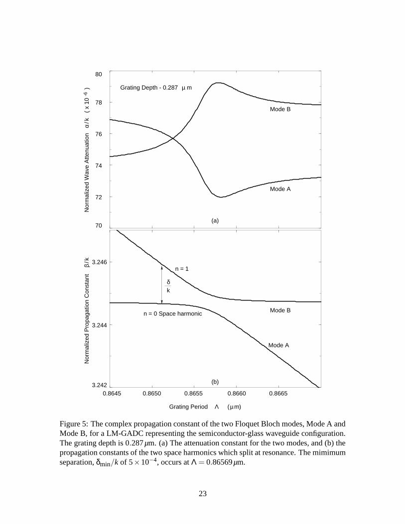
The complex propagation constants for the two modes of the LM-GADC are shown inFig. 5 for a grating depth of 0.287 µm. The space harmonic n = 0 of mode A interacts withthe n = 1 space harmonic of mode B. This interaction point corresponds to the intersectionpoint I0,1 of Fig. 3. The propagation constants of the two modes split, Fig. 5(b), as

7

they approach resonance while the attenuation curves (Fig. 5(b)) cross. The minimumvalue of δmin/k ≈ 5×10−4 occurs at the grating period Λ = 0.86569µm. Using Eq. (12),assuming the minimum value of δ, the calculated coupling length is Lc ≈ 1.5mm, which isapproximately 1,790 grating periods. However, this estimated coupling length is too largebecause the modal attenuation affects the true coupling length. (The optimized couplinglength, discussed later, is about 1.25 mm, or about 1,440 grating periods.)

As can be seen from Fig. 5(a), the curves representing the attenuation constants cross atΛ≈ 0.86525µm, somewhat below the resonant point when δ is a minimum (Λ≈ 0.86569µm).Near resonance, the attenuation of mode B has a maximum, while the attenuation of modeA is a minimum. These two features are usually exhibited in a resonant system and indi-cates that a stop band occurs for mode B while mode A is in a passband.

The two key layer thicknesses affecting the coupling length and the amount of powercoupled from the region in the vicinity of sub-waveguide S to the region in the vicinity ofsub-waveguide G, are (1) grating depth and (2) the thickness of the spacer layer (Table II).In the present example, the tooth height is 0.287µm and the grating period is approximately0.86µm.

Because of the presence of the grating layer, the fields of the LM-GADC and the GADCstructures are expanded in an infinite number of space harmonics. While the complete fielddistributions consist of the summation of all space harmonics, there are only a few spaceharmonics with significant amplitudes. Away from resonance, only one space harmonic isdominant, whereas at least two space harmonics have significant amplitudes at the resonantcondition. For mode A, the n = 0 and -1 space harmonics are dominant, while other spaceharmonics are negligible. For mode B, the n = 0 and 1 space harmonics are dominant, whilethe others are negligible.

The complete field pattern can be obtained by the summation of all spatial harmon-ics. Figure 6 shows the total field distributions of mode A and mode B, where mode Arepresents the “in-phase” (no zero-crossings of the electric field distribution between thewaveguides) solution, and mode B displays the “out-of-phase” (a single zero-crossing ofthe electric field distribution between the waveguides) solution. (The imaginary part of thefields are also shown in the figure.) Note that both field distributions have almost identicalintensities in both sub-waveguides. It is the inclusion of the space harmonics that producesthe “in-phase” and “out-of-phase” solutions for the two modes. The addition or subtractionof these two solutions puts the tandem waveguide power in either sub-waveguide S or sub-waveguide G. In other words, a linear combination of the two modes can produce a fielddistribution with most of the light in one of the waveguides. The fine structure on the fieldpatterns in Fig. 6 indicates the excitation of higher-order space harmonics.

The propagation characteristics shown in Fig. 5 are plotted as a function of the gratingperiod. Although this is not a true “ω−β” plot it illustrates modal characteristics as a func-tion of grating period. A “classic dispersion” curve is shown in Fig. 7. Again, the figurerepresents the characteristics in the neighborhood of the intersection point I0,1. The pairs ofdots correspond to specific values of the grating period. The dots and corresponding fielddistributions are given for three different grating periods, (1) a Λ value below resonance,(2) a Λ value at resonance and (3) a Λ value above resonance. Below resonance, mode

8

A is confined to the semiconductor sub-waveguide and mode B is confined to the glasssub-waveguide. Above resonance, mode A has most of its power confined to the glasssub-guide and mode B is confined to the semiconductor sub-guide.

The two modes switch their “mode profile signatures” as they progress through res-onance. It is interesting to note that the modal group velocity is vg = c/(dβ/dk) for thepropagating mode. (All space harmonics associated with the mode propagate with the samegroup velocity vg. This implies the mode maintains a given shape as it propagates.) Thedefinition of the group velocity implies dβ/dk behaves as an effective group index, ng. Thevalue of the effective group index is a measure of where the optical intensities are confined.For example, the effective group index of a mode confined to the glass waveguide is ap-proximately equal to the refractive index of the glass. (Because ng > 1, the slope of thecurves in Fig. 7 can never be greater than 1.) Below resonance, the effective group indexof mode A, ngA, is approximately equal to the effective group index of mode B, ngB, aboveresonance. Likewise, ngB, below resonance is approximately equal to ngA above reso-nance. In the former case, a majority of the optical power is confined to the semiconductor,whereas, in the latter case, a majority of the optical power is confined to the glass guide.As the two modes progress through resonance, they reach the point when ngA = ngB. Thiscondition implies that each mode has very similar optical distributions. Specifically, the“in-phase” and “out-of-phase” modes have nearly identical intensity patterns.

V. The Coupling MechanismExcitation of the coupler from an external source such as a connecting waveguide will

generate all of the modes of the LM-GADC. To minimize scattering at their interface, thefields of the two waveguides (exciting and coupler waveguides) must have similar shapes.A “smooth transition” can be obtained with an exciting guide that is almost identical to theLM-GADC waveguide. In the present case, the exciting waveguide will be assumed to beidentical to the coupler waveguide, except the input waveguide will not have a grating at thesemiconductor/glass interface (see Fig. 1). The input waveguide has two trapped modes:one mode’s fields are predominantly confined to the semiconductor sub-waveguide, whilethe second mode will have fields predominantly confined to the glass sub-waveguide. Whenthe exciting waveguide contains an incident field composed of only the semiconductormode, the fields in the semiconductor portion match the fields of each of the two couplermodes. Near resonance, both coupler modes will be excited with almost equal amplitudes,and the field in the glass sub-waveguide is negligible.

The two Floquet-Bloch modes of the LM-GADC are in general nonorthogonal. As theypropagate in the z direction, there may be an exchange of power from one mode to the other.(This power exchange between modes is not our present concern.) The primary focus hereis to understand how to transfer or “couple” power between the two sub-waveguides. Inparticular, we discuss how to transform an initial power distribution with power concen-trated in the semiconductor sub-waveguide, say at z = 0, to a transverse power distributionwith power concentrated in the glass sub-waveguide, at the distant point z = Lg. Physically,the LM-GADC will be excited from the semiconductor/glass waveguide section using thesemiconductor mode that is incident from the z < 0 region. The excitation at z = 0 dictateshow the power is partitioned between the two Bloch modes.

9

At resonance, the field shapes of the Bloch modes have special and interesting charac-teristics. (Neither Bloch mode can be normalized in the transverse direction, −∞ < x < ∞,using their intensity distributions. However, we have normalized their intensity patterns inthe vicinity of the tandem waveguide using finite limits on x, including layers 2 through15 of Table II.) By choosing a particular phase of one mode relative to the other, bothBloch modes have peak values (real parts) in the sub-waveguide S, however, the fields inthe sub-waveguide G are out of phase.

To appreciate the special shapes of the complex LM-GADC modes at resonance, weexplore how a combination of the two modes allows an excellent match to an input ex-citing field. The general solution to the fields in the coupler must be written as a linearcombination of the two Floquet-Bloch modes as

Ey(x,z) = aA fA(x,z)e−γAz +aB fB(x,z)e−γBz, (13)

where aA and aB are the expansion coefficients that measure the partition of the power intothe modes. For the present discussion, assume the coupler is excited with all the power inthe semiconductor sub-waveguide. At the input z = 0, the field in the coupler is obtainedby summing the two modes of Fig. 6, implying aA = aB = 1/2. As the two modes progressalong the z direction, the continuously evolving field shape amounts to a redistribution ofpower in the sub-waveguides of the composite waveguide.

We estimate the powers PA and PB in sub-waveguides S and G respectively, as [2]

PS = −12

Re� ∞

0EyH∗

x dx,

PG = −12

Re� 0

−∞EyH∗

x dx.

For the structure whose dispersion characteristics are shown in Fig. 5, the percentage ofthe total input power coupled to the glass waveguide, as a function of grating length Lg,is shown in Fig. 8. At the excitation point, the total waveguide power is concentrated inthe semiconductor side. The power is transferred to the glass as the LM-GADC modespropagate.

Figure 8 also shows the coupled power versus grating length with various grating peri-ods of the LM-GADC structure of Fig. 1. The curves indicate that the maximum couplingdrops as the coupler is detuned from resonance. At resonance, we obtain the maximumcoupled power and the optimum coupling length. Off resonance, both the coupled powerand the optimum coupling length are reduced. As shown in Fig. 8, the maximum coupledpower is greater than 40 % with a coupling length of 1.25 mm, and the optimum gratingperiod is 0.8657µm.

We now determine the coupling characteristics from the raw dispersion data of Fig. 7.Due to the “symmetric” and “asymmetric” shapes of the two fields illustrated in Fig. 6, itis convenient to write the fields in terms of two functions s(x) and g(x). The function s(x)represents the field distribution in the semiconductor sub-waveguide while g(x) represents

10

the field in the glass sub-waveguide. In addition, the two functions satisfy:

s(x) ≈ 0 for x ∈ Glass sub-waveguide,

g(x) ≈ 0 for x ∈ Semiconductor sub-waveguide.

It is interesting to note that the function s(x) is approximately equivalent to the field distri-bution of the semiconductor mode in the absence of a grating layer. Similarly, the functiong(x) is approximately equivalent to the field distribution of the glass mode in the absenceof the grating layer. Thus, when the LM-GADC is excited with the “semiconductor mode”,the excitation field shape is s(x). On the other hand, when the LM-GADC is excited with a“glass mode”, the excitation field shape is g(x).

The overall field distribution as given by Eq. (1) across the layers can be written as

f (x,z) = f (i)(x,z) for x ∈ ith layer.

Due to the nature of the field shapes as shown in Fig. 6, the Floquet-Bloch modes can beapproximated with the two dominant space harmonics of modes A and B. These dominantspace harmonics are characterized by the two functions s(x) and g(x),

fA(x,z) = s(x)+g(x)e jKz,

fB(x,z) = s(x)e− jKz−g(x).

Using the approximate expressions for the modes, the total field becomes (putting aA =aB = 1/2)

Ey(x,z) =12[s(x)+g(x)e jKz]e−γAz +

12[s(x)e− jKz

−g(x)]e−γBz.

At an arbitrary position, z, the total field becomes

Ey(x,z) =12

{

[s(x)+g(x)e jKz]+ [s(x)e− jKz−g(x)]e−(γB−γA)z

}

e−γAz.

As seen from Fig. 5, the attenuation coefficients of the two modes near resonance haveapproximately equal values (αA ≈ αB), so that the term αB −αA can be dropped, so thatthe exponent γB − γA = αB−αA + j(βB−βA) ≈ j(δ−K). The resulting field simplifies to

Ey(x,z) = e− j 12 δz

[

s(x)cos(12

δz)+ jg(x)e jKz sin(12

δz)

]

e−γAz. (17)

The first term in the brackets characterizes the field in the semiconductor guide while thesecond term characterizes the field in glass. To find the optimum coupling length, wherethe power in the glass guide is maximized, the magnitude of the second term must be max-imized relative to z, and the optimum z value will represent the best coupling length. In theoptimization process, the phase term exp[ j(K −βa)z] is dropped because the envelope am-plitude, characterized by sin(δz/2) exp(−αAz), is to be maximized. After simplification,the optimum coupling length Lc is found to be a solution to the transcendental equation

tanδ2

Lc =δ

2α. (18)

11

(Because the attenuation coefficients are approximately equal, the term αA has been re-placed by α.) Although the results obtained for the optimum coupling length assumesapproximately equal values of attenuation for both modes, a similar result can be obtainedwhen modal attenuations are different. In the limiting case of α → 0, Eq. (18) reduces toEq. (12).

To determine the coupling length for optimum power transfer for the structure describedin Table II, the value of the deviation coefficient δ = δmin = (5× 10−4)k and α ≈ (7.5×10−5)k are substituted into Eq. (18). These optimum values produce a coupling length ofLc ≈ 1.25mm which agrees with the value obtained from the numerical computations forthe coupling efficiency, shown in Fig. 8.

VI. OptimizationThe coupling depends on the combination of the difference between βA

0 and βB1 and the

attenuation coefficients of the modes. In many cases modal attenuation is a dominant factorresulting in low power transfer. When one mode attenuates much faster than the second, itis difficult to achieve high percentages of power transfer. A major result of this analysis isthat the attenuation of the Bloch modes plays a significant role in determining the optimumcoupling length in grating couplers.

The field distributions of the two Floquet-Bloch modes evolve as the ω−β plot pro-gresses through resonance. As the modes exchange their “signatures”, there is a singlepoint where both have the same group velocity and the deviation wavenumber δ is min-imized. This implies that they have almost equal intensity shapes. When this conditionoccurs, the usual “in-phase” and “out-of-phase” fields allow for a linear combination ofthe modes to produce a distribution of power which is concentrated in one waveguide orthe other. If the modes are combined (say added) with equal amplitudes, the resultingfield places the power in the semiconductor sub-waveguide. Likewise if the modes aresubtracted, the power is placed in the glass sub-waveguide. Furthermore, when one modevanishes over a distance smaller than π/δ, only one mode remains and field shape in thecomposite waveguide is invariant with z. Therefore, to find the maximum coupling, theattenuation characteristics of the two modes must be evaluated.

The key parameter that affects modal attenuation is the coupling strength. (Both thegrating depth, period and grating duty cycle affect the coupling strength. A 50 % duty cycleis used in all of our calculations.) Figure 9 shows the normalized attenuation coefficient asa function of grating depth for modes A and B. The grating period is fixed at 0.8670µm,which is well below the resonant condition. In addition, the thickness of layer 6 (seeTable II), is 0.3175µm. It should be noted that other values of the grating period and spacerlayer thickness produce a differently shaped curve, but all resulting curves are similar inthat their maximum and minimum values of α lie in ranges similar to those shown in Fig. 9.Namely, mode A has minimum α values at grating depths near 0 and 0.3µm. Attenuationof mode B is rather insensitive to grating depth.

Grating depths that produce the best coupling efficiency are in those ranges where αA isvery close to αB. In addition, these ranges correspond to the smallest values of attenuation.These best ranges occur at grating depths near 0 and 0.3µm. At grating depths near 0,

12

the coupling strength is very small which produces very small δmin values. These smallδmin values extrapolate to relatively long coupling lengths Lc that are typically impractical.When the grating depth is increased, the difference of the two attenuations αA and αB

increases. Although the LM-GADC structure changes coupling strength with an increasedtooth height, the low values of either 1/αA or 1/αB, the length when the mode amplitudedrops to 1/e of its initial value, are smaller than computed values of 1/δmin where the bestcoupling length occurs. Thus, the mode attenuates before a 180◦ relative phase changeoccurs. For tooth heights near zero, the coupling efficiency is generally below 10 percentwhile for grating depths near 0.3µm, the coupling efficiency is about 40 percent.

The coupled power to the glass region as shown in Fig. 8 reaches a peak value and thendrops back to near zero. This classic oscillation (with auxiliary attenuation due to leakageof power) occurs because power shifts back and forth between the two sub-waveguides.The power in the semiconductor sub-waveguide oscillates out of phase relative to the powerin the glass sub-waveguide. At the optimum coupling length when the power in the glasspeaks, the power in the semiconductor waveguide is at a minimum.

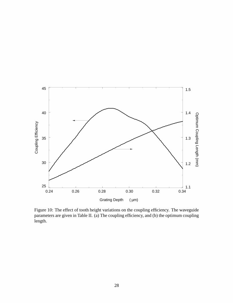
Figure 10 shows the coupled power as a function of tooth height, assuming the param-eters given in Table II. In fact the optimum value of approximately 40 % or about 4 dB,occurs at a grating depth of 0.287µm. The optimum coupling length is Lc ≈ 1.25mm. Eventhough the coupling length Lc increases for grating depths above 0.287µm, the coupling ef-ficiency drops.

When the grating period Λ, or the wavelength λ is changed, the optimum coupling isreduced. For example, in Fig. 8, the grating period Λ = 0.8657µm requires the coupler tohave a length of Lg = 1.25mm. If the actual length is different from 1.25 mm, the couplingefficiency will be decreased.

A characteristic of the LM-GADC is its frequency selectivity or its narrow-bandedproperty. Using the results of Fig. 8, the coupling efficiency for the 1.25 mm length LM-GADC as a function wavelength deviation δλ about λ = 1.55µm is shown in Fig. 11. We

find the FWHP of the coupling bandwidth is about 9◦

A.

VII ConclusionFloquet-Bloch analysis has been been applied to the study of LM-GADCs that are fab-

ricated with two very different materials such as semiconductor materials (refractive indexof approximately 3.2) and glass (refractive index of about 1.48). The complex propagationconstants of the two lowest-order modes of the tandem waveguide system are determinedversus various parameters such as grating period and grating depth. Assuming the semicon-ductor and glass waveguide dimensions and refractive indices are those given in Table II,the optimum grating depth is 0.28µm. The resulting coupling efficiency is about 40 per-cent, or about 4 dB, and the optimum coupling length is 1.25 mm. The grating period atthe optimum is about 0.86µm.

The coupling efficiency obtained by this method is applicable to the two dimensionalmodel where the slab has infinite extension in the lateral direction. Generally, slab modelsare applicable to similar three dimensional structures when the widths of the modes in the

13

lateral (y-axis) dimension are large compared to the widths in the transverse (x-direction)dimension.

The simple LM-GADC is not an efficient coupler compared to the GADC. While theGADC of Table I can transfer almost 100 percent of its power from one region (first sub-waveguide) to a second region (second sub-waveguide), the LM-GADC of Table II cantransfer only about half of its input power from one guide to a second guide. The majorreason for this difference is due to the fact that the LM-GADC has more radiation loss andthe corresponding modal attenuation plays a dominant role in determining the optimumtransfer length. By incorporating multilayer reflective stacks in the substrate, we expect thecoupling efficiency can be increased to 70%. In the present examples, the modal attenuationof the LM-GADC of Table II is about one order of magnitude greater than the modalattenuation of the GADC of Table I. The LM-GADC losses are due mainly to powerleaking to the substrate.

Finally, Floquet-Bloch modes exchange “signatures” as they progress through reso-nance. The classical coupling length (when losses are negligible such as for the GADC),is determined from the minimum longitudinal propagation constant separation, δmin, us-ing Eq. (12). When losses become significant (such as with the LM-GADC), the couplinglength must be determined from Eq. (18).

14

References

[1] D. Marcuse, “Radiation loss of grating-assisted directional coupler,” IEEE J. Quan-tum Electron., vol. QE-26, no. 4, pp. 675–684, Apr. 1990.

[2] N. H. Sun, J. K. Butler, G. A. Evans, L. Pang, and P. Congdon, “Analysis of grating-assisted directional couplers using floquet bloch theory,” IEEE J. Lightwave Tech.,vol. 15, no. 12, pp. 2301–2315, Dec. 1997.

[3] D. Marcuse, “Directional couplers made of nonidentical asymmetric slabs. part i:Synchronous couplers,” IEEE J. Lightwave Tech., vol. LT-5, no. 1, pp. 113–118, Jan.1987.

[4] D. Marcuse, Theory of Dielectric Oprical Waveguides, Academic Press, San Diego,2nd ed. edition, 1991.

[5] W. P. Huang and H. A. Haus, “Power exchange in grating-assisted couplers,” IEEEJ. Lightwave Tech., vol. LT-7, no. 6, pp. 920–924, June 1989.

[6] H. A. Haus, W. P. Huang, S. Kawakami, and N. A. Whitaker, “Coupled-mode theoryof optical waveguides,” IEEE J. Lightwave Tech., vol. LT-5, no. 1, pp. 16–23, Jan.1987.

[7] W. P. Huang, B. E. Little, and S. K. Chaudhuri, “A new approach to grating-assistedcouplers,” IEEE J. Lightwave Tech., vol. LT-9, no. 6, pp. 721–727, June 1991.

[8] W. P. Huang and J. W. Y. Lit, “Nonorthogonal coupled-mode theory of grating-assisted codirectional couplers,” IEEE J. Lightwave Tech., vol. LT-9, no. 7, pp. 845–852, July 1991.

[9] W. P. Huang, J. Hong, and Z. M. Mao, “Improved coupled-mode formulation basedon composite mode for parallel grating-assisted co-directional couplers,” IEEE J.Quantum Electron., vol. QE-29, no. 11, pp. 2805–2812, Nov. 1993.

[10] W. P. Huang, “Coupled-mode theory for optical waveguides: An overview,” J. Opt.Soc. Am. A, vol. 11, no. 3, pp. 963–983, Mar. 1994.

[11] B. E. Little, W. P. Huang, and S. K. Chaudhuri, “A multiple-scale analysis of grating-assisted couplers,” IEEE J. Lightwave Tech., vol. LT-9, no. 10, pp. 1254–1263, Oct.1991.

[12] B. E. Little and H. A. Haus, “A variational coupled-mode theory for periodic waveg-uides,” IEEE J. Quantum Electron., vol. QE-31, no. 12, pp. 2258–2264, Dec. 1995.

[13] B. E. Little, “A variational coupled-mode theory including radiation loss for gratingassisted couplers,” IEEE J. Lightwave Tech., vol. LT-14, no. 2, pp. 188–195, Feb.1996.

15

[14] V. M. N. Passaro and M. N. Aremise, “Analysis of radiation loss in grating-assistedco-directional couplers,” IEEE J. Quantum Electron., vol. QE-31, no. 9, pp. 1691–1697, Sept. 1995.

[15] W. P. Huang and H. Hong, “A transfer matrix approach based on local normal modesfor coupled waveguides with periodic perturbations,” IEEE J. Lightwave Tech., vol.LT-10, no. 10, pp. 1367–1375, Oct. 1992.

[16] S. T. Peng, T. Tamir, and H. L. Bertoni, “Theory of periodic dielectric waveguides,”IEEE Trans. Microwave Theory Tech., vol. MTT-23, no. 1, pp. 123–133, Jan. 1975.

[17] K. C. Chang, V. Shah, and T. Tamir, “Scattering and guiding of waves by dielectricgratings with arbitrary profiles,” J. Opt. Soc. Am., vol. 70, pp. 804–813, July 1980.

[18] G. Hadjicostas, J. K. Butler, G. A. Evans, N. W. Carlson, and R. Amantea, “A numer-ical investigation of wave interactions in dielectric waveguides with periodic surfacecorrugations,” IEEE J. Quantum Electron., vol. QE-26, no. 5, pp. 893–902, May1990.

[19] J. K. Butler, W. E. Ferguson, G. A. Evans, P. J. Stabile, and A. Rosen, “A bound-ary element technique applied to the analysis of waveguides with periodic surfacecorrugations,” IEEE J. Quantum Electron., vol. QE-28, no. 7, pp. 1701–1709, July1992.

[20] R. L. Burden and J. D. Faires, Numerical Analysis, PWS-KENT, Boston, fourthedition, 1984.

16

Layer Thickness(µm) Refractive Index

1 Superstrate ∞ 3.1802 Sub-waveguide B 0.200 3.2823 Cladding 1.450 3.1804 Grating 0.010 3.180/3.2825 Step 0.450 3.2826 Sub-waveguide A 0.257 3.4507 Substrate ∞ 3.180

Table I: The parameters of grating assisted directional couplers using two similar sub-waveguides.[1] The free-space wavelength is λ0 = 1.5µm. “Sub-waveguide A” includeslayers 5 and 6 while “sub-waveguide B” includes layer 2.

17

Layer Thickness(µm) Refractive Index

1 Glass Cladding ∞ 1.4482 Glass Cladding 3.0000 1.4483 Glass Waveguide 5.0000 1.4584 Glass Cladding 1.0000 1.4485 Grating Layer 0.2870 3.165/1.4486 Spacer 0.3175 3.1657 Confining Layer 0.1200 3.3868 Quantum Well 0.0090 3.5329 Barrier 0.0100 3.38610 Quantum Well 0.0090 3.53211 Barrier 0.0100 3.38612 Quantum Well 0.0090 3.53213 Barrier 0.0100 3.38614 Quantum Well 0.0090 3.53215 Confining Layer 0.1200 3.38616 Substrate Cladding 1.0000 3.16517 Substrate ∞ 3.165

Table II: The parameters of grating assisted directional couplers using two different sub-waveguides. Sub-waveguide S consists of layers 7 through 15, while sub-waveguide Gconsists of layer 3. The free-space wavelength is λ0 = 1.55µm.

18

2

2

2

Semiconductor Waveguide

Glass Bottom Clad

SiO

P-DopedSiO

SiO

Semiconductor Top Clad

Glass Waveguide

Glass Top Clad

Semiconductor Bottom Clad

g

x

z

L

Figure 1: The cross section of an integrated semiconductor-glass waveguide. The gratingis etched into the semiconductor cladding region and the glass waveguide is deposited overthe grating. The grating assists in coupling light from the semiconductor sub-waveguide tothe glass sub-waveguide and vice versa.

19

1.4481.458

1.4481.458

-1 0 1 2 3 4 5 6

Transverse Direction x ( m)

1

2

3

4R

efra

ctiv

e In

dex

Pro

file

µ

Grating Region

Semiconductor Waveguide Region

Glass Waveguide Region

Figure 2: The refractive index profile of the semiconductor-glass waveguide configuration.The bottom of the grating is the orgin.

20

I-4,-3

I-2,-1

I-1,0 I

0,1I-2,-3

n = 0n = 1

n = -2n = -1

k Λ

β Λ0 2π−2π−4π 4π

Substrate

Superstrate

FWR

FWR

Mode A

Mod

e B

Figure 3: The kinematic properties of the co-directional coupling of two Floquet-Blochmodes. Mode A represents the mode of the “semiconductor waveguide”, while Mode B isthe mode of the “glass waveguide.”

21

kδ

mµ

14.00 14.02 14.04 14.06 14.083.2972

3.2974

3.2976

3.2977

3.2975

3.2973

0

2

4

6

8

10

Nor

mal

ized

Pro

paga

tion

Con

stan

t/k

βN

orm

aliz

ed W

ave

Atte

nuat

ion

α/k

( x

10)

-8

Grating Period ( m)µΛ

Mode B

Mode A

Mode A

Mode B

(b)

(a)

n = 0 Spaceharmonic

n = 1

Grating Depth - 0.01

Figure 4: The complex propagation constant of the two Floquet Bloch modes, mode Aand mode B, for a GADC. The grating depth is 0.01µm. (a) The modal x =attenuationcoefficients which cross, and (b) the propagation constants of the two space harmonicswhich split at resonance. The minimum separation , δmin/k of 6.5× 10−5, occurs at Λ =14.041µm.

22

Nor

mal

ized

Pro

paga

tion

Con

stan

tβ

/kN

orm

aliz

ed W

ave

Atte

nuat

ion

/k(

x 10

)α

-6

δk

mµ

0.86453.242

80

Grating Period ( m)Λ µ

Mode B

Mode A

(a)

(b)

Mode A

Mode B

70

74

78

72

76

3.244

3.246

0.8650 0.8655 0.8660 0.8665

n = 1

n = 0 Space harmonic

Grating Depth - 0.287

Figure 5: The complex propagation constant of the two Floquet Bloch modes, Mode A andMode B, for a LM-GADC representing the semiconductor-glass waveguide configuration.The grating depth is 0.287µm. (a) The attenuation constant for the two modes, and (b) thepropagation constants of the two space harmonics which split at resonance. The mimimumseparation, δmin/k of 5×10−4, occurs at Λ = 0.86569µm.

23

-2 0 2 4 6 8

Lateral Distance x ( µ

Fie

ld A

mpl

itude

s (A

rbitr

ary

Uni

ts)

Mode A (Re Part)

Mode B (Re Part)

Mode B (Im Part)

Mode A (Im Part)

m)

Figure 6: The optical field distribution at resonance. Mode A represents the “in-phase”mode while B is the “out-of-phase” mode. The term Re is for the real part of the field andIm stands for the imaginary part.

24

−2 0 2 4 6 8

−2 0 2 4 6 8

−2 0 2 4 6 8

−2 0 2 4 6 8

−2 0 2 4 6 8

−2 0 2 4 6 8

11.363.500

Normalized Propagation Constant βΛ

Nor

mal

ized

Wav

enum

ber

k

Mode A

Mode B

3.505

3.510

3.515

11.37 11.38 11.39 11.40 11.41

Λ

Figure 7: The “ω−β” diagram at the intersection I0,1. The field inserts in the figure are thereal parts of the fields. The corresponding imaginary parts, not shown, are relatively small.

25

Λ = 0.8657 µGrating Period

m

0 0.5 1.0 1.5 2.0

0.8656

0.8655

0.8654

0.8653

0

10

20

30

40

Cou

plin

g E

ffici

ency

Grating Length L (mm)g

Figure 8: The coupling efficiency as a function of propagation distance.

26

µm

µm

0 0.1 0.2 0.3 0.4 0.50

5

10

15

Mode A

Mode B

Grating Period - 0.8670

(

Nor

mal

ized

Mod

al A

ttenu

atio

nα

/k(

x 10

)-3

)Grating Depth

Figure 9: The normalized modal attenuation for the LM-GADC as a function of toothheight. The grating period is fixed at 0.8670µm. The grating period chosen for this calcu-lation is not near the resonance condition.

27

0.26 0.28 0.30 0.32 0.340.24

µ(

1.1

1.2

1.3

1.4

1.5

Cou

plin

g E

ffici

ency

Optim

um C

oupling Length (mm

)

25

30

35

40

45

m)Grating Depth

Figure 10: The effect of tooth height variations on the coupling efficiency. The waveguideparameters are given in Table II. (a) The coupling efficiency, and (b) the optimum couplinglength.

28

Free-Space Wavelength Deviation from Resonance (Angstroms)δλ

Resonant Wavelengthλ = 1.55 µm L = 1.25 mmg

Grating Length

-20 -10 0 10 200

10

20

40

30

Cou

plin

g E

ffici

ency

Figure 11: The coupling efficiency about the resonant wavelength, λ = 1.55µm. The reso-nant grating period is Λ = 0.86569µm.

29