Social Vulnerability Assessment for Landslide Hazards ... - MDPI
ORIGINAL PAPER
GIS-based frequency ratio and index of entropy modelsfor landslide susceptibility assessment in the Caspian forest,northern Iran
A. Jaafari • A. Najafi • H. R. Pourghasemi •
J. Rezaeian • A. Sattarian
Received: 2 July 2013 / Revised: 26 October 2013 / Accepted: 1 December 2013
� Islamic Azad University (IAU) 2013
Abstract This study presents a landslide susceptibility
assessment for the Caspian forest using frequency ratio
and index of entropy models within geographical infor-
mation system. First, the landslide locations were identi-
fied in the study area from interpretation of aerial
photographs and multiple field surveys. 72 cases (70 %)
out of 103 detected landslides were randomly selected for
modeling, and the remaining 31 (30 %) cases were used
for the model validation. The landslide-conditioning fac-
tors, including slope degree, slope aspect, altitude,
lithology, rainfall, distance to faults, distance to streams,
plan curvature, topographic wetness index, stream power
index, sediment transport index, normalized difference
vegetation index (NDVI), forest plant community, crown
density, and timber volume, were extracted from the
spatial database. Using these factors, landslide suscepti-
bility and weights of each factor were analyzed by fre-
quency ratio and index of entropy models. Results showed
that the high and very high susceptibility classes cover
nearly 50 % of the study area. For verification, the
receiver operating characteristic (ROC) curves were
drawn and the areas under the curve (AUC) calculated.
The verification results revealed that the index of entropy
model (AUC = 75.59 %) is slightly better in prediction
than frequency ratio model (AUC = 72.68 %). The
interpretation of the susceptibility map indicated that
NDVI, altitude, and rainfall play major roles in landslide
occurrence and distribution in the study area. The land-
slide susceptibility maps produced from this study could
assist planners and engineers for reorganizing and plan-
ning of future road construction and timber harvesting
operations.
Keywords Forest road construction � Mountainous
terrain � Slope stability � Susceptibility modeling
Introduction
Landslides are the movement of a mass of rock, debris, or
soil along a downward slope, due to gravitational pull (Das
et al. 2012). The reasons for landslides are many, complex,
convoluted, and every so often unknown (Yalcin et al.
2011). The significance of forestry activities such as road
construction and timber harvesting in slope imbalance
causing frequent occurrence of landslides is widely
acknowledged (e.g., Larsen and Parks 1997). Timber har-
vesting in the north mountainous forest (Caspian region) of
Iran moved on to steep terrain in the 1980s and early 1990s
without a systematic approach for the identification of
unstable terrain or down slope risks associated with road
construction and timber harvesting. History has shown that
roads with improper terrain stability assessment in this area
can cause extensive and severe landslides (IPBO 2000).
A. Jaafari � A. Najafi (&)
Department of Forestry, Faculty of Natural Resources, Tarbiat
Modares University (TMU), P.O. Box: 64414-356, Noor,
Mazandaran, Iran
e-mail: [email protected]
H. R. Pourghasemi
Department of Watershed Management Engineering, Faculty of
Natural Resources, Tarbiat Modares University (TMU), Noor,
Iran
J. Rezaeian
Department of Industrial Engineering, Mazandaran University of
Science and Technology, Babol, Iran
A. Sattarian
Department of Forestry, Faculty of Agriculture and Natural
Resources, Gonbad Kavous University, Gonbad Kavous, Iran
123
Int. J. Environ. Sci. Technol.
DOI 10.1007/s13762-013-0464-0
High landslide frequency has resulted in large financial,
social, and environmental costs in this area. This trend is
not likely to decline soon; some estimates suggest that
significant portions of forestland in the northern Iran are
prone to mass wasting and the forestry activities that reg-
ularly happening on these lands have the potential to
accelerate landslide rates and magnitudes (IPBO 2000). It
is therefore critical to understand landslides and to find
measures to mitigate subsequent losses to future landslides.
Through scientific analyses, geoscientists and engineers
can assess and predict landslide-prone areas, offering
potential measures to decrease landslide damages (Oh and
Pradhan 2011). Landslide susceptibility mapping (LSM)
could be the basis for decision-making to help citizens,
planners, and engineers to reduce the losses caused by
current and future landslides by means of prevention,
mitigation, and avoidance (Feizizadeh and Blaschke 2013).
Various techniques and methods have been proposed and
developed for the LSM purposes. They can be categorized
into four groups depending on the modeling approach:
statistical, analytic, deterministic, and heuristic techniques
(Guzzetti et al. 1999). Each has its inherent advantages and
limitations. For example, when study area is large, appli-
cation of analytic methods is almost impossible (Pradhan
2013). The levels of landslide susceptibility determined by
statistical methods are drastically affected by the accuracy
of mapping of different conditioning factors and landslide
inventory (Guzzetti et al. 1999). Das et al. (2012) address
the issue of LSM along road corridors using Bayesian
logistic regression models. They state that ‘‘heuristic
approaches, in many instances, are biased as they depend
on expert knowledge. Statistical methods, on the other
hand, help to remove the bias of expert judgment and
express the variability present in the datasets. Logistic
regression is a robust and straightforward statistical method
that is relatively easy to handle.’’ Yilmaz (2009), in a
comparative study, argues that ‘‘input process, calculations,
and output process are very simple and can be readily
understood in the frequency ratio model; however, logistic
regression and neural networks require the conversion of
data to ASCII or other formats. It is also very hard to
process the large amount of data in the statistical package.
On the other hand, all the three models have relatively
similar accuracies.’’ In general, these methods give rise to
qualitative and quantitative maps of the landslide hazard
areas, and the spatial results are appealing (Bui et al. 2012).
Independent of the modeling approach, the first step for
assessing and managing of any landslide-prone area is to
provide a landslide inventory map. The next step is the
production of a LSM, which includes the spatial distribu-
tion of conditioning factors. This will allow landslide-
prone areas to be delimited and indicate where landslides
may likely occur in the future. The third step involves the
creation of a landslide hazard map, which, in contrast to
LSM, includes a temporal framework, with the probability
of landslide occurrence within a specified period of time.
The final step is the production of a landslide risk map,
describing the expected annual cost of landslide damage
throughout the affected area. Ultimately, all four maps are
used to delimit and present zones of landslide susceptibil-
ity, hazard, and risk, respectively. A landslide zone is
essentially a division of the land into areas and their clas-
sification according to degrees of actual or potential land-
slide hazard or susceptibility (Kamp et al. 2008).
The study was carried out in the Educational and Exper-
imental Forest of Tarbiat Modares University (EEFTMU) in
July–October 2012. The main objective of this study was to
provide managers and foresters with a comprehensive
assessment of landslide susceptibility in forestlands. For this
purpose, we used frequency ratio and index of entropy
models within a GIS environment. These models exploit
information obtained from an inventory map, and a wide
variety of conditioning factors to predict where landslides
may occur in future. Furthermore, we provided a validation
of the landslide susceptibility maps prepared for the study
area. This study has practical implications for forest man-
agement and is novel; in that, it is the first replicated study in
north mountainous forest of Iran to comprehensively assess
the terrain stability for forestry activities.
Materials and methods
Study area
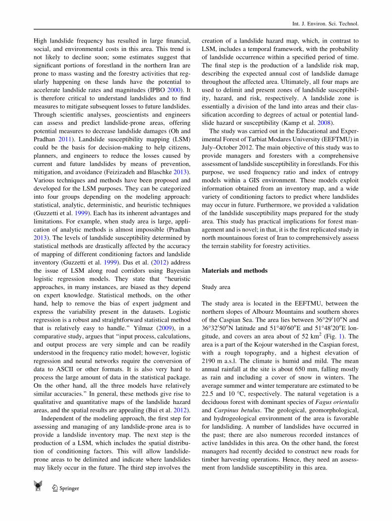
The study area is located in the EEFTMU, between the
northern slopes of Albourz Mountains and southern shores
of the Caspian Sea. The area lies between 36�2901000N and
36�3205000N latitude and 51�4006000E and 51�4802000E lon-
gitude, and covers an area about of 52 km2 (Fig. 1). The
area is a part of the Kojour watershed in the Caspian forest,
with a rough topography, and a highest elevation of
2190 m a.s.l. The climate is humid and mild. The mean
annual rainfall at the site is about 650 mm, falling mostly
as rain and including a cover of snow in winters. The
average summer and winter temperature are estimated to be
22.5 and 10 �C, respectively. The natural vegetation is a
deciduous forest with dominant species of Fagus orientalis
and Carpinus betulus. The geological, geomorphological,
and hydrogeological environment of the area is favorable
for landsliding. A number of landslides have occurred in
the past; there are also numerous recorded instances of
active landslides in this area. On the other hand, the forest
managers had recently decided to construct new roads for
timber harvesting operations. Hence, they need an assess-
ment from landslide susceptibility in this area.
Int. J. Environ. Sci. Technol.
123
Data used
Landslide inventory map
Landslide inventory mapping is the systematic mapping of
existing landslides in the study area using different tech-
niques, such as field survey, aerial photograph, and satellite
image interpretation, and literature search for historical
landslide records (Ozdemir and Altural 2013). The land-
slide inventory map for our study area was compiled
through aerial photographs interpretation and field-based
inspection. In the aerial photographs, historical landslides
could be observed as breaks in the forest canopy, bare soil,
or geomorphological features, such as head- and side-
Fig. 1 Location of the study area with landslide location map
Int. J. Environ. Sci. Technol.
123
scarps, flow tracks, and soil deposits and debris deposits
below a scar (Oh and Pradhan 2011). Given the abundant
overstory and understory vegetation in the study forest, we
also conducted multiple field surveys and observations to
produce a more detailed and reliable landslide inventory
map. A total of 103 landslides were detected in the study
area (Fig. 1). 72 cases (70 %) out of 103 detected land-
slides were randomly selected for modeling, and the
remaining 31 (30 %) cases were used for the model vali-
dation purposes (Mohammady et al. 2012; Pourghasemi
et al. 2013).
Landslide-conditioning factors
The fundamental step for developing the predictive
models of landslide occurrence is the recognition of the
factors that are responsible for landsliding. The number
of conditioning factors may range from only a few
numbers to several (Mohammady et al. 2012; Pourgha-
semi et al. 2012b; Papathanassiou et al. 2012). The
selection of these factors mainly depends on the avail-
ability of data for the study area and the relevance with
respect to landslide occurrences (Papathanassiou et al.
2012). According to the Ayalew and Yamagishi (2005),
in GIS-based studies, the selected factors should be
operational, complete, non-uniform, measurable, and
non-redundant. In this study, we considered a total of 15
landslide-conditioning factors. ArcGIS and SAGA GIS
were employed to generate required conditioning factors.
Slope degree, slope aspect, altitude, plan curvature,
topographic wetness index (TWI), stream power index
(SPI), and sediment transport index (STI) were extracted
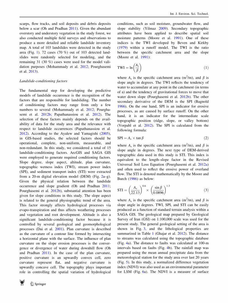
from a 20-m digital elevation model (DEM) (Fig. 2a–g).
Given the physical relation between the landslide
occurrence and slope gradient (Oh and Pradhan 2011;
Pourghasemi et al. 2012b), substantial attention has been
given for slope conditions in this study. The slope aspect
is related to the general physiographic trend of the area.
This factor strongly affects hydrological processes via
evapo-transpiration and thus affects weathering processes
and vegetation and root development. Altitude is also a
significant landslide-conditioning factor because it is
controlled by several geological and geomorphological
processes (Dai et al. 2001). Plan curvature is described
as the curvature of a contour line formed by intersecting
a horizontal plane with the surface. The influence of plan
curvature on the slope erosion processes is the conver-
gence or divergence of water during downhill flow (Oh
and Pradhan 2011). In the case of the plan curvature,
positive curvature is an upwardly convex cell, zero
curvature represent flat, and negative curvature is
upwardly concave cell. The topography plays important
role in controlling the spatial variation of hydrological
conditions, such as soil moisture, groundwater flow, and
slope stability (Yilmaz 2009). Secondary topographic
attributes have been applied to describe spatial soil
moisture patterns (Moore et al. 1991). One of these
indices is the TWI developed by Beven and Kirkby
(1979) within a runoff model. The TWI is the ratio
between the specific catchment area and the slope
(Moore et al. 1991):
TWI ¼ lnAs
b
� �ð1Þ
where As is the specific catchment area (m2/m), and b is
slope angle in degrees. The TWI reflects the tendency of
water to accumulate at any point in the catchment (in terms
of a) and the tendency of gravitational forces to move that
water down slope (Pourghasemi et al. 2012b). The other
secondary derivative of the DEM is the SPI (Bagnold
1966). On the one hand, SPI is an indicator for erosive
processes, as are caused by surface runoff. On the other
hand, it is an indicator for the intermediate scale
topographic position (ridge, slope, or valley bottom)
(Vorpahl et al. 2012). The SPI is calculated from the
following formula:
SPI ¼ As � tan b ð2Þ
where As is the specific catchment area (m2/m), and b is
slope angle in degrees. The next type of DEM-derived
topographic data used in this study is STI. This index is
equivalent to the length–slope factor in the Revised
Universal Soil Loss Equation (Pourghasemi et al. 2012a)
and often used to reflect the erosive power of overland
flow. The STI is denoted mathematically by the Moore and
Burch (1986) as below:
STI ¼ As
22:13
� �0:6
� sin b0:0896
� �1:3
ð3Þ
where As is the specific catchment area (m2/m), and b is
slope angle in degrees. TWI, SPI, and STI can be easily
produced as a function of standard terrain analysis within a
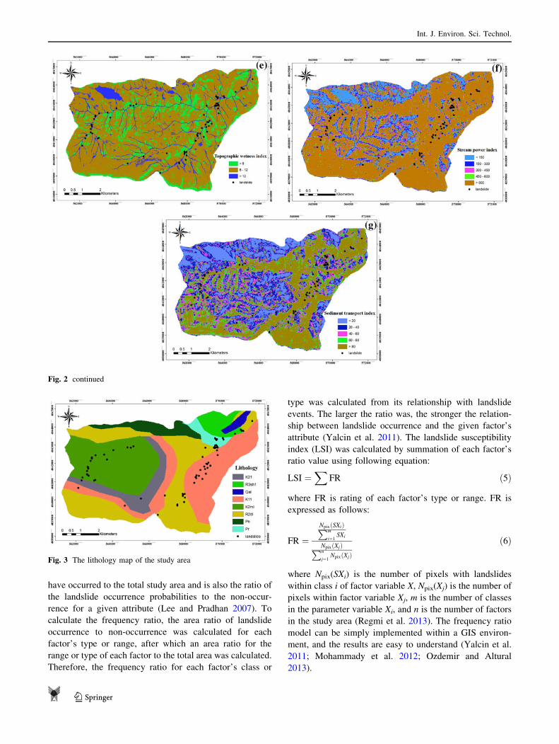
SAGA GIS. The geological map prepared by Geological
Survey of Iran (GSI) on 1:100,000 scale was used for the
present study. The general geological setting of the area is
shown in Fig. 3, and the lithological properties are
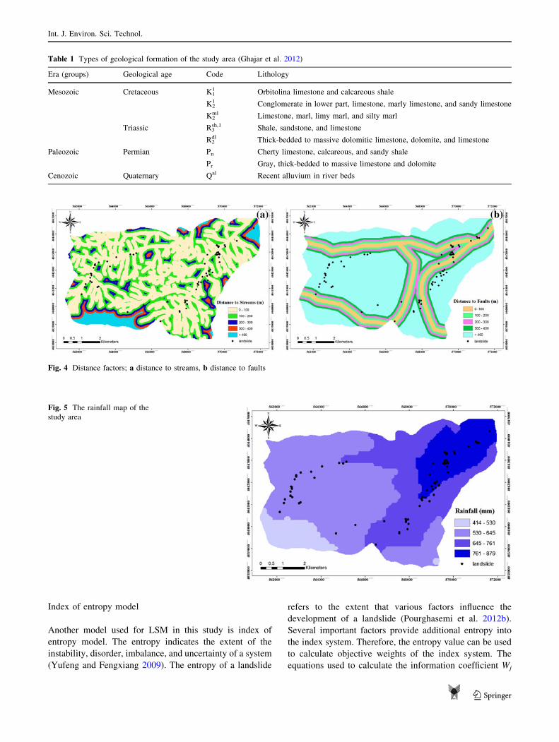
summarized in Table 1 (Ghajar et al. 2012). The distance
to streams was calculated using the topographic database
(Fig. 4a). The distance to faults was calculated at 100-m
intervals based on faults (Fig. 4b). The rainfall map was
prepared using the mean annual precipitate data from the
meteorological station for the study area over last 20 years
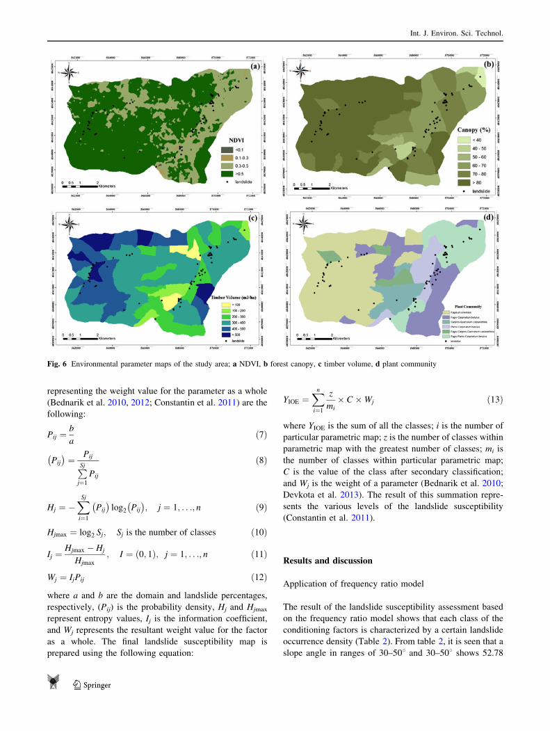
(Fig. 5). In this study, a normalized difference vegetation
index (NDVI) was also used as an environmental parameter
for LSM (Fig. 6a). The NDVI is a measure of surface
Int. J. Environ. Sci. Technol.
123

reflectance and gives a quantitative estimate of vegetation
growth and biomass (Hall et al. 1995). The NDVI is
defined as follows:
NDVI ¼ ðIR� RÞðIRþ RÞ ð4Þ
where IR is the infrared portion of the electromagnetic
spectrum, and R is the red portion of the electromagnetic
spectrum. Low values of the NDVI (0.1 and below)
indicate barren areas, sand, or snow. Moderate values
(0.2–0.3) represent shrub and grasslands, whereas high
values (0.6–0.8) correspond to temperate and tropical
rainforests (Yilmaz and Keskin 2009). Forest canopy,
timber volume, and plant community are also significant
environmental parameters considered in this study
(Fig. 6b–d). Given the important role of forest canopy in
controlling many aspects of forest ecosystem dynamics
(Sefidi et al. 2011), this index is incorporated as vital
variables when modeling forest responses to the pressing
issues (Didham and Fagan 2004). Timber volume (m3/ha)
has long been the most commonly used forestland attri-
bute for providing information for the development of
management strategies. Forest plant community is known
to introduce some mechanical changes through soil rein-
forcement and slope loading (Abdi et al. 2010). The
increase in soil strength due to root reinforcement has
great potential to reduce the rate of landslide occurrence
(Yalcin et al. 2011).
All the above-mentioned landslide-conditioning factors
were stored in raster format with a cell size of 20 9 20 m
and were overlaid with the landslide inventory map for
the application of frequency ratio and index of entropy
models.
Landslide susceptibility mapping (LSM)
Frequency ratio model
Mass movement and landslide-controlling factors are
generally assumed to be similar to those observed in the
past. If this assumption holds true, one can predict future
slides occurring in a non-specified time span (Feizizadeh
and Blaschke 2013). The frequency ratio model is based on
the assumption that future landslides will occur at similar
conditions to those in the past (Lee and Pradhan 2007). The
frequency ratio is the ratio of the area where landslides
Fig. 2 Topographic parameter maps of the study area; a slope degree, b slope aspect, c altitude, d plan curvature; e topographic wetness index;
f stream power index; g sediment transport index
Int. J. Environ. Sci. Technol.
123
have occurred to the total study area and is also the ratio of
the landslide occurrence probabilities to the non-occur-
rence for a given attribute (Lee and Pradhan 2007). To
calculate the frequency ratio, the area ratio of landslide
occurrence to non-occurrence was calculated for each
factor’s type or range, after which an area ratio for the
range or type of each factor to the total area was calculated.
Therefore, the frequency ratio for each factor’s class or
type was calculated from its relationship with landslide
events. The larger the ratio was, the stronger the relation-
ship between landslide occurrence and the given factor’s
attribute (Yalcin et al. 2011). The landslide susceptibility
index (LSI) was calculated by summation of each factor’s
ratio value using following equation:
LSI ¼X
FR ð5Þ
where FR is rating of each factor’s type or range. FR is
expressed as follows:
FR ¼NpixðSXiÞPm
i¼1SXi
NpixðXjÞPn
j¼1NpixðXjÞ
ð6Þ
where Npix(SXi) is the number of pixels with landslides
within class i of factor variable X, Npix(Xj) is the number of
pixels within factor variable Xj, m is the number of classes
in the parameter variable Xi, and n is the number of factors
in the study area (Regmi et al. 2013). The frequency ratio
model can be simply implemented within a GIS environ-
ment, and the results are easy to understand (Yalcin et al.
2011; Mohammady et al. 2012; Ozdemir and Altural
2013).
Fig. 2 continued
Fig. 3 The lithology map of the study area
Int. J. Environ. Sci. Technol.
123
Index of entropy model
Another model used for LSM in this study is index of
entropy model. The entropy indicates the extent of the
instability, disorder, imbalance, and uncertainty of a system
(Yufeng and Fengxiang 2009). The entropy of a landslide
refers to the extent that various factors influence the
development of a landslide (Pourghasemi et al. 2012b).
Several important factors provide additional entropy into
the index system. Therefore, the entropy value can be used
to calculate objective weights of the index system. The
equations used to calculate the information coefficient Wj
Table 1 Types of geological formation of the study area (Ghajar et al. 2012)
Era (groups) Geological age Code Lithology
Mesozoic Cretaceous K11 Orbitolina limestone and calcareous shale
K21 Conglomerate in lower part, limestone, marly limestone, and sandy limestone
K2ml Limestone, marl, limy marl, and silty marl
Triassic R3sh,1 Shale, sandstone, and limestone
R2dl Thick-bedded to massive dolomitic limestone, dolomite, and limestone
Paleozoic Permian Pn Cherty limestone, calcareous, and sandy shale
Pr Gray, thick-bedded to massive limestone and dolomite
Cenozoic Quaternary Qal Recent alluvium in river beds
Fig. 4 Distance factors; a distance to streams, b distance to faults
Fig. 5 The rainfall map of the
study area
Int. J. Environ. Sci. Technol.
123
representing the weight value for the parameter as a whole
(Bednarik et al. 2010, 2012; Constantin et al. 2011) are the
following:
Pij ¼b
að7Þ
Pij
� �¼ Pij
PSj
j¼1
Pij
ð8Þ
Hj ¼ �XSj
i¼1
Pij
� �log2 Pij
� �; j ¼ 1; . . .; n ð9Þ
Hjmax ¼ log2 Sj; Sj is the number of classes ð10Þ
Ij ¼Hjmax � Hj
Hjmax
; I ¼ 0; 1ð Þ; j ¼ 1; . . .; n ð11Þ
Wj ¼ IjPij ð12Þ
where a and b are the domain and landslide percentages,
respectively, (Pij) is the probability density, Hj and Hjmax
represent entropy values, Ij is the information coefficient,
and Wj represents the resultant weight value for the factor
as a whole. The final landslide susceptibility map is
prepared using the following equation:
YIOE ¼Xn
i¼1
z
mi
� C �Wj ð13Þ
where YIOE is the sum of all the classes; i is the number of
particular parametric map; z is the number of classes within
parametric map with the greatest number of classes; mi is
the number of classes within particular parametric map;
C is the value of the class after secondary classification;
and Wj is the weight of a parameter (Bednarik et al. 2010;
Devkota et al. 2013). The result of this summation repre-
sents the various levels of the landslide susceptibility
(Constantin et al. 2011).
Results and discussion
Application of frequency ratio model
The result of the landslide susceptibility assessment based
on the frequency ratio model shows that each class of the
conditioning factors is characterized by a certain landslide
occurrence density (Table 2). From table 2, it is seen that a
slope angle in ranges of 30–508 and 30–508 shows 52.78
Fig. 6 Environmental parameter maps of the study area; a NDVI, b forest canopy, c timber volume, d plant community
Int. J. Environ. Sci. Technol.
123
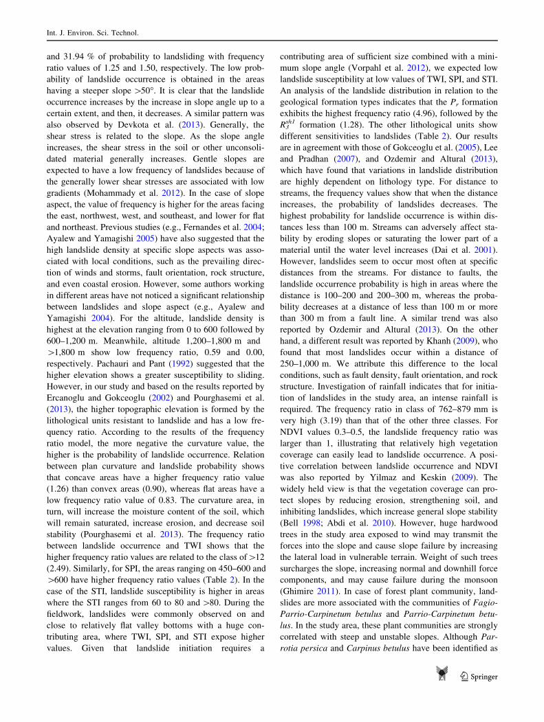
and 31.94 % of probability to landsliding with frequency
ratio values of 1.25 and 1.50, respectively. The low prob-
ability of landslide occurrence is obtained in the areas
having a steeper slope [50�. It is clear that the landslide
occurrence increases by the increase in slope angle up to a
certain extent, and then, it decreases. A similar pattern was
also observed by Devkota et al. (2013). Generally, the
shear stress is related to the slope. As the slope angle
increases, the shear stress in the soil or other unconsoli-
dated material generally increases. Gentle slopes are
expected to have a low frequency of landslides because of
the generally lower shear stresses are associated with low
gradients (Mohammady et al. 2012). In the case of slope
aspect, the value of frequency is higher for the areas facing
the east, northwest, west, and southeast, and lower for flat
and northeast. Previous studies (e.g., Fernandes et al. 2004;
Ayalew and Yamagishi 2005) have also suggested that the
high landslide density at specific slope aspects was asso-
ciated with local conditions, such as the prevailing direc-
tion of winds and storms, fault orientation, rock structure,
and even coastal erosion. However, some authors working
in different areas have not noticed a significant relationship
between landslides and slope aspect (e.g., Ayalew and
Yamagishi 2004). For the altitude, landslide density is
highest at the elevation ranging from 0 to 600 followed by
600–1,200 m. Meanwhile, altitude 1,200–1,800 m and
[1,800 m show low frequency ratio, 0.59 and 0.00,
respectively. Pachauri and Pant (1992) suggested that the
higher elevation shows a greater susceptibility to sliding.
However, in our study and based on the results reported by
Ercanoglu and Gokceoglu (2002) and Pourghasemi et al.
(2013), the higher topographic elevation is formed by the
lithological units resistant to landslide and has a low fre-
quency ratio. According to the results of the frequency
ratio model, the more negative the curvature value, the
higher is the probability of landslide occurrence. Relation
between plan curvature and landslide probability shows
that concave areas have a higher frequency ratio value
(1.26) than convex areas (0.90), whereas flat areas have a
low frequency ratio value of 0.83. The curvature area, in
turn, will increase the moisture content of the soil, which
will remain saturated, increase erosion, and decrease soil
stability (Pourghasemi et al. 2013). The frequency ratio
between landslide occurrence and TWI shows that the
higher frequency ratio values are related to the class of[12
(2.49). Similarly, for SPI, the areas ranging on 450–600 and
[600 have higher frequency ratio values (Table 2). In the
case of the STI, landslide susceptibility is higher in areas
where the STI ranges from 60 to 80 and [80. During the
fieldwork, landslides were commonly observed on and
close to relatively flat valley bottoms with a huge con-
tributing area, where TWI, SPI, and STI expose higher
values. Given that landslide initiation requires a
contributing area of sufficient size combined with a mini-
mum slope angle (Vorpahl et al. 2012), we expected low
landslide susceptibility at low values of TWI, SPI, and STI.
An analysis of the landslide distribution in relation to the
geological formation types indicates that the Pr formation
exhibits the highest frequency ratio (4.96), followed by the
R3sh1 formation (1.28). The other lithological units show
different sensitivities to landslides (Table 2). Our results
are in agreement with those of Gokceoglu et al. (2005), Lee
and Pradhan (2007), and Ozdemir and Altural (2013),
which have found that variations in landslide distribution
are highly dependent on lithology type. For distance to
streams, the frequency values show that when the distance
increases, the probability of landslides decreases. The
highest probability for landslide occurrence is within dis-
tances less than 100 m. Streams can adversely affect sta-
bility by eroding slopes or saturating the lower part of a
material until the water level increases (Dai et al. 2001).
However, landslides seem to occur most often at specific
distances from the streams. For distance to faults, the
landslide occurrence probability is high in areas where the
distance is 100–200 and 200–300 m, whereas the proba-
bility decreases at a distance of less than 100 m or more
than 300 m from a fault line. A similar trend was also
reported by Ozdemir and Altural (2013). On the other
hand, a different result was reported by Khanh (2009), who
found that most landslides occur within a distance of
250–1,000 m. We attribute this difference to the local
conditions, such as fault density, fault orientation, and rock
structure. Investigation of rainfall indicates that for initia-
tion of landslides in the study area, an intense rainfall is
required. The frequency ratio in class of 762–879 mm is
very high (3.19) than that of the other three classes. For
NDVI values 0.3–0.5, the landslide frequency ratio was
larger than 1, illustrating that relatively high vegetation
coverage can easily lead to landslide occurrence. A posi-
tive correlation between landslide occurrence and NDVI
was also reported by Yilmaz and Keskin (2009). The
widely held view is that the vegetation coverage can pro-
tect slopes by reducing erosion, strengthening soil, and
inhibiting landslides, which increase general slope stability
(Bell 1998; Abdi et al. 2010). However, huge hardwood
trees in the study area exposed to wind may transmit the
forces into the slope and cause slope failure by increasing
the lateral load in vulnerable terrain. Weight of such trees
surcharges the slope, increasing normal and downhill force
components, and may cause failure during the monsoon
(Ghimire 2011). In case of forest plant community, land-
slides are more associated with the communities of Fagio-
Parrio-Carpinetum betulus and Parrio-Carpinetum betu-
lus. In the study area, these plant communities are strongly
correlated with steep and unstable slopes. Although Par-
rotia persica and Carpinus betulus have been identified as
Int. J. Environ. Sci. Technol.
123
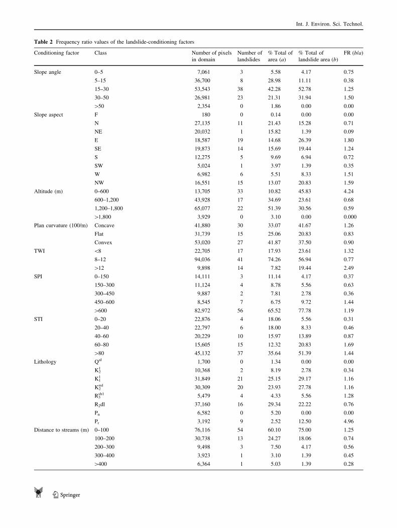
Table 2 Frequency ratio values of the landslide-conditioning factors
Conditioning factor Class Number of pixels
in domain
Number of
landslides
% Total of
area (a)
% Total of
landslide area (b)
FR (b/a)
Slope angle 0–5 7,061 3 5.58 4.17 0.75
5–15 36,700 8 28.98 11.11 0.38
15–30 53,543 38 42.28 52.78 1.25
30–50 26,981 23 21.31 31.94 1.50
[50 2,354 0 1.86 0.00 0.00
Slope aspect F 180 0 0.14 0.00 0.00
N 27,135 11 21.43 15.28 0.71
NE 20,032 1 15.82 1.39 0.09
E 18,587 19 14.68 26.39 1.80
SE 19,873 14 15.69 19.44 1.24
S 12,275 5 9.69 6.94 0.72
SW 5,024 1 3.97 1.39 0.35
W 6,982 6 5.51 8.33 1.51
NW 16,551 15 13.07 20.83 1.59
Altitude (m) 0–600 13,705 33 10.82 45.83 4.24
600–1,200 43,928 17 34.69 23.61 0.68
1,200–1,800 65,077 22 51.39 30.56 0.59
[1,800 3,929 0 3.10 0.00 0.000
Plan curvature (100/m) Concave 41,880 30 33.07 41.67 1.26
Flat 31,739 15 25.06 20.83 0.83
Convex 53,020 27 41.87 37.50 0.90
TWI \8 22,705 17 17.93 23.61 1.32
8–12 94,036 41 74.26 56.94 0.77
[12 9,898 14 7.82 19.44 2.49
SPI 0–150 14,111 3 11.14 4.17 0.37
150–300 11,124 4 8.78 5.56 0.63
300–450 9,887 2 7.81 2.78 0.36
450–600 8,545 7 6.75 9.72 1.44
[600 82,972 56 65.52 77.78 1.19
STI 0–20 22,876 4 18.06 5.56 0.31
20–40 22,797 6 18.00 8.33 0.46
40–60 20,229 10 15.97 13.89 0.87
60–80 15,605 15 12.32 20.83 1.69
[80 45,132 37 35.64 51.39 1.44
Lithology Qal 1,700 0 1.34 0.00 0.00
K21 10,368 2 8.19 2.78 0.34
K11 31,849 21 25.15 29.17 1.16
K2ml 30,309 20 23.93 27.78 1.16
R3sh1 5,479 4 4.33 5.56 1.28
R2dl 37,160 16 29.34 22.22 0.76
Pn 6,582 0 5.20 0.00 0.00
Pr 3,192 9 2.52 12.50 4.96
Distance to streams (m) 0–100 76,116 54 60.10 75.00 1.25
100–200 30,738 13 24.27 18.06 0.74
200–300 9,498 3 7.50 4.17 0.56
300–400 3,923 1 3.10 1.39 0.45
[400 6,364 1 5.03 1.39 0.28
Int. J. Environ. Sci. Technol.
123

a potential restoration species for revegetating steep slopes
(Abdi et al. 2010), their relatively sparse crown makes
them relatively ineffective at insuring slope stability (Sefidi
et al. 2011). For timber volume, the results show that the
range between 0–100, 200–300, and 300–400 m3/ha is
relatively favorable (highly susceptible) for landslide
occurrence. Their frequency ratios are 1.23, 1.02, and 1.28,
respectively. With regard to forest canopy, the classes of
50–60 % and [80 % seem to have the lowest impact on
landslide occurrence. Their frequency ratios are 0.00 and
0.63, respectively. In forest ecosystems, canopy acts as a
shelter and reduces soil erosion and landslide occurrence.
The final result of frequency ratio model is a LSI map, in
which the LSI values vary from 7.91 to 47.48.
Application of index of entropy model
In landslide susceptibility mapping using frequency ratio
model, it was assumed that all the conditioning factors
carry equal weight in determining the vulnerability status
of the pixels. However, a factor is considered as non-
existing and is ignored for the study when it has the same
value throughout the study area. According to the Sharma
et al. (2010), ‘‘if 90 % of the study area has same value and
only 10 % of the study area has different values for a
particular parameter, the overall role of this parameter in
determining the vulnerability status in the study area
should be less than any other parameter whose values
exhibit consistent and uniform variation throughout the
Table 2 continued
Conditioning factor Class Number of pixels
in domain
Number of
landslides
% Total of
area (a)
% Total of
landslide area (b)
FR (b/a)
Distance to faults (m) 0–100 15,442 6 12.19 8.33 0.68
100–200 13,567 13 10.71 18.06 1.69
200–300 13,266 13 10.48 18.06 1.72
300–400 11,891 4 9.39 5.56 0.59
[400 72,473 36 57.23 50.00 0.87
Rainfall (mm) 414–529 9,220 0 7.28 0.00 0.00
530–645 63,812 23 50.39 31.94 0.63
646–761 35,427 16 27.97 22.22 0.79
762–879 18,180 33 14.36 45.83 3.19
NDVI \0.1 321 0 0.25 0.00 0.00
0.1–0.3 463 0 0.37 0.00 0.00
0.3–0.5 11,265 40 8.90 55.56 6.25
[0.5 114,590 32 90.49 44.44 0.49
Forest canopy (%) 0–40 1,226 1 0.97 1.39 1.43
40–50 2,864 2 2.26 2.78 1.23
50–60 5,370 0 4.24 0.00 0.00
60–70 21,252 20 16.78 27.78 1.66
70–80 29,185 25 23.05 34.72 1.51
[80 66,742 24 52.70 33.33 0.63
Timber volume (m3/ha) 0–100 4,355 3 3.44 4.17 1.21
100–200 5,309 1 4.19 1.39 0.33
200–300 22,387 13 17.68 18.06 1.02
300–400 56,153 41 44.34 56.94 1.28
400–500 28,252 11 22.31 15.28 0.68
[500 10,183 3 8.04 4.17 0.52
Plant community Fagetum orientalis 54,858 20 43.32 27.78 0.64
Fagio-Carpinetum betulus 24,930 12 19.69 16.67 0.85
Carpino-Quercetum castaneifolia 10,131 2 8.00 2.78 0.35
Parrio-Carpinetum betulus 9,561 8 7.55 11.11 1.47
Fagio-Carpino-Quercetum
castaneifolia
5,837 1 4.61 1.39 0.30
Fagio-Parrio-Carpinetum betulus 21,322 29 16.84 40.28 2.39
Int. J. Environ. Sci. Technol.
123
Table 3 Entropy values of the landslide-conditioning factors
Conditioning factor Class a b Pij (Pij) Hj Hj max Ij Wj
Slope angle 0–5 5.58 4.17 0.747 0.193 1.844 2.322 0.206 0.160
5–15 28.98 11.11 0.383 0.099
15–30 42.28 52.78 1.248 0.322
30–50 21.31 31.94 1.499 0.387
[50 1.86 0.00 0.000 0.000
Slope aspect F 0.14 0.00 0.000 0.000 2.709 3.170 0.145 0.129
N 21.43 15.28 0.713 0.089
NE 15.82 1.39 0.088 0.011
E 14.68 26.39 1.798 0.224
SE 15.69 19.44 1.239 0.155
S 9.69 6.94 0.716 0.089
SW 3.97 1.39 0.350 0.044
W 5.51 8.33 1.511 0.189
NW 13.07 20.83 1.594 0.199
Altitude (m) 0–600 10.82 45.83 4.235 0.769 1.011 2.000 0.494 0.681
600–1,200 34.69 23.61 0.681 0.124
1,200–1,800 51.39 30.56 0.595 0.108
[1,800 3.10 0.00 0.000 0.000
Plan curvature (100/m) Concave 33.07 41.67 1.260 0.422 1.560 1.585 0.016 0.016
Flat 25.06 20.83 0.831 0.278
Convex 41.87 37.50 0.896 0.300
TWI \8 17.93 23.61 1.317 0.288 1.427 1.585 0.100 0.152
8–12 74.26 56.94 0.767 0.168
[12 7.82 19.44 2.488 0.544
SPI 0–150 11.14 4.17 0.374 0.094 2.103 2.322 0.094 0.075
150–300 8.78 5.56 0.632 0.159
300–450 7.81 2.78 0.356 0.089
450–600 6.75 9.72 1.441 0.361
[600 65.52 77.78 1.187 0.298
STI 0–20 18.06 5.56 0.308 0.064 2.081 2.322 0.104 0.099
20–40 18.00 8.33 0.463 0.097
40–60 15.97 13.89 0.869 0.182
60–80 12.32 20.83 1.691 0.354
[80 35.64 51.39 1.442 0.302
Lithology Qal 1.34 0.00 0.339 0.035 2.073 3.000 0.309 0.373
K21 8.19 2.78 1.284 0.133
K11 25.15 29.17 1.160 0.120
K2ml 23.93 27.78 1.161 0.120
R3sh1 4.33 5.56 0.000 0.000
R2dl 29.34 22.22 0.757 0.078
Pn 5.20 0.00 0.000 0.000
Pr 2.52 12.50 4.959 0.513
Distance to streams (m) 0–100 60.10 75.00 1.248 0.381 2.145 2.322 0.076 0.050
100–200 24.27 18.06 0.744 0.227
200–300 7.50 4.17 0.556 0.170
300–400 3.10 1.39 0.448 0.137
[400 5.03 1.39 0.276 0.084
Int. J. Environ. Sci. Technol.
123
study area.’’ In this study, we employed index of entropy to
reduce the unevenness among the parameters and thereby
to provide realistic status of their impact on the landslide
susceptibility within the study area. The results show that
each class of the conditioning factors is characterized by a
certain landslide occurrence density Pij (Eq. 7 and
Table 3). Overall, the most important factors controlling
the distribution of landslides were derived and are pre-
sented in Table 3. The findings based on entropy approach
show that NDVI, altitude, and rainfall are the most
important factors which explain better the landslide
occurrence and distribution in study area. The final land-
slide susceptibility map was developed using the Eq. (13)
as follow:
Table 3 continued
Conditioning factor Class a b Pij (Pij) Hj Hj max Ij Wj
Distance to faults (m) 0–100 12.19 8.33 0.683 0.123 2.181 2.322 0.061 0.067
100–200 10.71 18.06 1.685 0.303
200–300 10.48 18.06 1.724 0.310
300–400 9.39 5.56 0.592 0.106
[400 57.23 50.00 0.874 0.157
Rainfall (mm) 414–529 7.28 0.00 0.000 0.000 1.198 2.000 0.401 0.463
530–645 50.39 31.94 0.634 0.137
646–761 27.97 22.22 0.794 0.172
762–879 14.36 45.83 3.193 0.691
NDVI \0.1 0.25 0.00 0.000 0.000 0.377 2.000 0.812 1.367
0.1–0.3 0.37 0.00 0.000 0.000
0.3–0.5 8.90 55.56 6.245 0.927
[0.5 90.49 44.44 0.491 0.073
Forest canopy (%) 0–40 0.97 1.39 1.435 0.222 2.259 2.585 0.126 0.136
40–50 2.26 2.78 1.228 0.190
50–60 4.24 0.00 0.000 0.000
60–70 16.78 27.78 1.655 0.256
70–80 23.05 34.72 1.507 0.233
[80 52.70 33.33 0.632 0.098
Timber volume (m3/ha) 0–100 3.44 4.17 1.212 0.240 2.448 2.585 0.053 0.045
100–200 4.19 1.39 0.331 0.066
200–300 17.68 18.06 1.021 0.202
300–400 44.34 56.94 1.284 0.254
400–500 22.31 15.28 0.685 0.136
[500 8.04 4.17 0.518 0.103
Plant community Fagetum orientalis 43.32 27.78 0.641 0.107 1.986 2.585 0.232 0.232
Fagio-Carpinetum betulus 19.69 16.67 0.847 0.141
Carpino-Quercetum castaneifolia 8.00 2.78 0.347 0.058
Parrio-Carpinetum betulus 7.55 11.11 1.472 0.245
Fagio-Carpino-Quercetum castaneifolia 4.61 1.39 0.301 0.050
Fagio-Parrio-Carpinetum betulus 16.84 40.28 2.392 0.399
YIOE ¼
slope degree� 0:16ð Þ þ slope aspect� 0:129ð Þ þ altitude � 0:681ð Þ þ plan curvature� 0:016ð Þþ TWI� 0:152ð Þ þ SPI� 0:075ð Þ þ STI� 0:099ð Þ þ lithology� 0:373ð Þ þ distance to streams� 0:05ð Þþ distance to faults � 0:067ð Þ þ rainfall� 0:463ð Þ þ NDVI� 1:367ð Þ þ forest canopy� 0:136ð Þþ timber volume� 0:045ð Þ þ forest plant community� 0:232ð Þ
0BBB@
1CCCA:
Int. J. Environ. Sci. Technol.
123
The final result of index of entropy model is a LSI map,
in which the LSI values vary from 1.5965 to 24.5357.
Landslide susceptibility maps
For visual interpretation of LSI maps, the data need to be
classified into categorical susceptibility classes. There are
many classification methods available, such as quantiles,
natural breaks, equal intervals, and standard deviations
(Ayalew and Yamagishi 2005). Generally, the selection of
classification methods depends on the distribution of the
landslide susceptibility indexes (Ayalew and Yamagishi
2005). For instance, if the data distribution is close to normal,
equal interval, or standard deviation, classifiers should be
used. If the data distribution has a positive or negative
skewness, the quantile or natural break distribution classifi-
ers could be chosen (Akgun et al. 2012). In this study, con-
sidering data distribution histogram, the quantile and natural
break classifiers were applied to the data. The comparison
results indicated that the quantile classifier was able to pro-
duce better results than the natural break classifier. There-
fore, the quantile data classification approach was chosen,
and the landslide susceptibility index maps were classified
into four susceptibility classes: low, moderate, high, and very
high (Pourghasemi et al. 2012b). According to the landslide
susceptibility map generated with the frequency ratio model
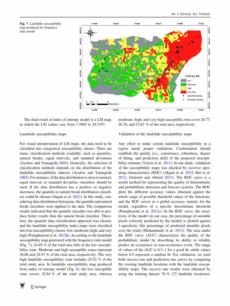
(Fig. 7), 24.49 % of the total area falls in the low suscepti-
bility zone. Moderate and high susceptible zones represent
26.06 and 24.93 % of the total area, respectively. The very
high landslide susceptibility zone includes 24.52 % of the
total study area. In landslide susceptibility map produced
from index of entropy model (Fig. 8), the low susceptible
zone covers 22.84 % of the total study area, whereas
moderate, high, and very high susceptible zone cover 26.77,
26.76, and 23.63 % of the total area, respectively.
Validation of the landslide susceptibility maps
Any effort to make certain landslide susceptibility in a
region needs proper validation. Confirmation should
establish the quality (i.e., consistency, robustness, degree
of fitting, and prediction skill) of the proposed suscepti-
bility estimate (Yalcin et al. 2011). In our study, validation
of the susceptibility maps was checked by receiver oper-
ating characteristics (ROC) (Akgun et al. 2012; Bui et al.
2012; Ozdemir and Altural 2013). The ROC curve is a
useful method for representing the quality of deterministic
and probabilistic detection and forecast systems. The ROC
plots the different accuracy values obtained against the
whole range of possible threshold values of the functions,
and the ROC serves as a global accuracy statistic for the
model, regardless of a specific discriminate threshold
(Pourghasemi et al. 2012c). In the ROC curve, the sensi-
tivity of the model (in our case, the percentage of unstable
pixels correctly predicted by the model) is plotted against
1-specificity (the percentage of predicted unstable pixels
over the total) (Mohammady et al. 2012). The area under
the ROC curve (AUC) characterizes the quality of the
probabilistic model by describing its ability to reliably
predict an occurrence or non-occurrence event. The range
of values of the AUC is 0.5–1 for a good fit, while values
below 0.5 represent a random fit. For validation, we used
both success rate and prediction rate curves by comparing
the existing landslide locations with the landslide suscep-
tibility maps. The success rate results were obtained by
using the training dataset 70 % (72 landslide locations).
Fig. 7 Landslide susceptibility
map produced by frequency
ratio model
Int. J. Environ. Sci. Technol.
123
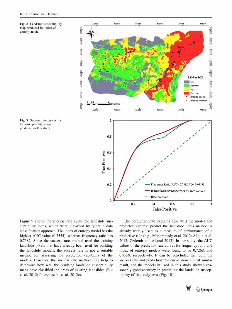
Figure 9 shows the success rate curve for landslide sus-
ceptibility maps, which were classified by quantile data
classification approach. The index of entropy model has the
highest AUC value (0.7554), whereas frequency ratio has
0.7382. Since the success rate method used the training
landslide pixels that have already been used for building
the landslide models, the success rate is not a suitable
method for assessing the prediction capability of the
models. However, the success rate method may help to
determine how well the resulting landslide susceptibility
maps have classified the areas of existing landslides (Bui
et al. 2012; Pourghasemi et al. 2012c).
The prediction rate explains how well the model and
predictor variable predict the landslide. This method is
already widely used as a measure of performance of a
predictive rule (e.g., Mohammady et al. 2012; Akgun et al.
2012; Ozdemir and Altural 2013). In our study, the AUC
values of the prediction rate curves for frequency ratio and
index of entropy models were found to be 0.7268, and
0.7559, respectively. It can be concluded that both the
success rate and prediction rate curve show almost similar
result, and the models utilized in this study showed rea-
sonably good accuracy in predicting the landslide suscep-
tibility of the study area (Fig. 10).
Fig. 8 Landslide susceptibility
map produced by index of
entropy model
Fig. 9 Success rate curves for
the susceptibility maps
produced in this study
Int. J. Environ. Sci. Technol.
123
As already mentioned, the natural break classifier was
also used to classify the LSI maps into categorical sus-
ceptibility classes. Furthermore, the obtained maps were
validated by ROC method. In the case of success rate, the
frequency ratio and index of entropy models showed the
AUC values of 0.7242, and 0.7195, respectively. For pre-
diction accuracy, the AUC values were 0.6977, and 0.6833,
respectively. The comparison results indicate that the
quantile classifier performs better than the natural break in
classification LSI maps produced in this study.
Conclusion
Landslides are the most frequent natural hazards in the
Caspian forest. However, progress in susceptibility map-
ping at the operational scale lags behind. This study
applied widely accepted models, frequency ratio, and index
of entropy, within a GIS environment for the purpose of
LSM. Although previous studies have applied these models
to produce LS maps, the efficiency and effectiveness of
which had not been evaluated in forestlands before the
present study. The ROC plots showed that the accuracy of
the LS maps produced by the frequency ratio and index of
entropy models was 72.68 and 75.59 %, respectively.
Furthermore, we have found the models relatively flexible
and easy to use. While complex models provide a basis for
building and consolidating scientific knowledge, simple
models are more useful and easily applied for land man-
agement purposes. One should always keep in mind that
‘‘simple is the best’’ in engineering applications. LSM
using GIS-based frequency ratio and index of entropy
models has the advantages of (1) allowing catchment-scale
assessment, (2) incorporating a wide range of the factors
thought to affect occurrence of landslide phenomena, and
(3) discriminating the considered factors to help the man-
agers to understand which factors are the most important to
trigger landslide phenomena.
The landslide susceptibility maps produced in this study
can provide a cheap and comprehensive assessment of the
study area for its capacity for supporting individual uses or
combination of uses, such as road construction and timber
harvesting. Managers and foresters can then make deci-
sions and prepare prescriptions that will have highly pre-
dictable results for producing sustainable products,
maintaining site quality, and substantially reducing risk of
any adverse impacts.
Acknowledgments This work was supported by the Tarbiat Mod-
ares University. Abdullah Abbasi, Sattar Ezzati, Hamed Asadi, and
Mostafa Adib are thanked for their assistance in field surveys. The
authors also express their sincere appreciation to the anonymous
reviewers for their helpful and valuable detailed comments and
suggestions.
References
Abdi E, Majnounian B, Genet M, Rahimi H (2010) Quantifying the
effects of root reinforcement of Persian Ironwood (Parrotia
persica) on slope stability; a case study: Hillslope of Hyrcanian
forests, northern Iran. Ecol Eng 36(10):1409–1416
Akgun A, Sezer EA, Nefesliogl HA, Gokceoglu C, Pradhan B (2012)
An easy-to-use MATLAB program (MamLand) for the assess-
ment of landslide susceptibility using a Mamdani fuzzy
algorithm. Comput Geosci 38:23–34
Fig. 10 Prediction rate curves
for the susceptibility maps
produced in this study
Int. J. Environ. Sci. Technol.
123
Ayalew L, Yamagishi H (2004) Slope movements in the Blue Nile
basin, as seen from landscape evolution perspective. Geomor-
phology 57:95–116
Ayalew L, Yamagishi H (2005) The application of GIS-based logistic
regression for landslide susceptibility mapping in the Kakuda–
Yahiko Mountains, Central Japan. Geomorphology 65(1–2):
15–31
Bagnold RA (1966) An Approach to the Sediment Transport Problem
from General Physics. USGS Professional Paper, Washington,
DC
Bednarik M, Magulova B, Matys M, Marschalko M (2010) Landslide
susceptibility assessment of the Kralovany–Liptovsky Mikulas
railway case study. Phys Chem Earth Parts A/B/C 35(3):162–171
Bednarik M, Yilmaz I, Marschalko M (2012) Landslide hazard and
risk assessment: a case study from the Hlohovec–Sered’landslide
area in south-west Slovakia. Nat Hazards 64(1):547–575
Bell FG (1998) Environmental geology: principles and practice.
Wiley-Blackwell, NY
Beven KJ, Kirkby MJ (1979) A physically-based variable contribut-
ing area model of basin hydrology. Hydrol Sci Bull 24:43–69
Bui TD, Pradhan B, Lofman O, Revhaug I, Dick OB (2012) Spatial
prediction of landslide hazards in Hoa Binh province (Vietnam):
a comparative assessment of the efficacy of evidential belief
functions and fuzzy logic models. Catena 96:28–40
Constantin M, Bednarik M, Jurchescu MC, Vlaicu M (2011)
Landslide susceptibility assessment using the bivariate statistical
analysis and the index of entropy in the Sibiciu Basin (Romania).
Environ Earth Sci 63:397–406
Dai FC, Lee CF, Xu ZW (2001) Assessment of landslide suscepti-
bility on the natural terrain of Lantau Island, Hong Kong.
Environ Geol 40(3):381–391
Das I, Stein A, Kerle N, Dadhwal VK (2012) Landslide susceptibility
mapping along road corridors in the Indian Himalayas using
Bayesian logistic regression models. Geomorphology 179:
116–125
Devkota KC, Regmi AD, Pourghasemi HR, Yoshida K, Pradhan B,
Ryu IC, Dhital MR, Althuwaynee OF (2013) Landslide suscep-
tibility mapping using certainty factor, index of entropy and
logistic regression models in GIS and their comparison at
Mugling–Narayanghat road section in Nepal Himalaya. Nat
Hazards 65:1–31
Didham RK, Fagan LL (2004) Forest Canopies. Encyclopedia of
forest science. Elsevier, Amsterdam, pp 68–80
Ercanoglu M, Gokceoglu C (2002) Assessment of landslide suscep-
tibility for a landslide-prone area (North of Yenice, NW Turkey)
by fuzzy approach. Environ Geol 41:720–730
Feizizadeh B, Blaschke T (2013) GIS-multicriteria decision analysis
for landslide susceptibility mapping: comparing three methods
for the Urmia lake basin, Iran. Nat Hazards 65:2105–2128
Fernandes NF, Guimaraes RF, Gomes RAT, Vieira BC, Montgomery
DR, Greenberg H (2004) Topographic controls of landslides in
Rio de Janeiro: field evidence and modelling. Catena
55:163–181
Ghajar I, Najafi A, Torabi SA, Khamehchiyan M, Boston K (2012)
An adaptive network-based fuzzy inference system for rock
share estimation in forest road construction. Croat J For Eng
33(2):313–328
Ghimire M (2011) Landslide occurrence and its relation with terrain
factors in the Siwalik Hills, Nepal: case study of susceptibility
assessment in three basins. Nat Hazards 56(1):299–320
Gokceoglu C, Sonmez H, Nefeslioglu HA, Duman TY, Can T (2005)
The 17 March 2005 Kuzulu landslide (Sivas, Turkey) and
landslide-susceptibility map of its near vicinity. Eng Geol
81:65–83
Guzzetti F, Carrara A, Cardinali M, Reichenbach P (1999) Landslide
hazard evaluation: a review of current techniques and their
application in a multi-scale study, Central Italy. Geomorphology
31:181–216
Hall FG, Towhshend JR, Engman ET (1995) Status of remote sensing
algorithms for estimation of land surface state parameters. Rem
Sens Environ 51:138–156
Iranian Plan and Budget Organization (IPBO) (2000) Guidelines for
design, execute and using forest roads No: 131, 2nd edn. Office
of the Deputy for Technical Affairs. Bureau of Technical Affairs
and Standards, 170 pp
Kamp U, Growley BJ, Khattak GA, Owen LA (2008) GIS-based
landslide susceptibility mapping for the 2005 Kashmir earth-
quake region. Geomorphology 101(4):631–642
Khanh NQ (2009) Landslide hazard assessment in muonglay,
Vietnam applying GIS and remote sensing. Dr.rer. nat. at the
Faculty of Mathematics and Natural Sciences Ernst-Moritz-
Arndt- University Greifswald. http://deposit.ddb.de/cgibin/dok
serv?idn=1009125575&dok_var=d1&dok_ext=pdf&filename=
1009125575.pdf
Larsen MC, Parks JE (1997) How wide is a road? The association of
roads and mass-wasting in a forested mountain environment.
Earth Surf Proc Land 22:835–848
Lee S, Pradhan B (2007) Landslide hazard mapping at Selangor,
Malaysia using frequency ratio and logistic regression models.
Landslides 4:33–41
Mohammady M, Pourghasemi HR, Pradhan B (2012) Landslide
susceptibility mapping at Golestan Province Iran: a comparison
between frequency ratio, Dempster-Shafer, and weights-of
evidence models. J Asian Earth Sci 61:221–236
Moore ID, Burch GJ (1986) Physical basis of the length-slope factor
in the Universal Soil Loss Equation. Soil Sci Soc Am J
50(5):1294–1298
Moore ID, Grayson RB, Ladson AR (1991) Digital terrain modeling:
a review of hydrological, geomorphological, and biological
applications. Hydrol Process 5:3–30
Oh HJ, Pradhan B (2011) Application of a neuro-fuzzy model to
landslide susceptibility mapping for shallow landslides in a
tropical hilly area. Comput Geosci 37:1264–1276
Ozdemir A, Altural T (2013) A comparative study of frequency ratio,
weights of evidence and logistic regression methods for landslide
susceptibility mapping: Sultan Mountains, SW Turkey. J Asian
Earth Sci 64:180–197
Pachauri AK, Pant M (1992) Landslide hazard mapping based on
geological attributes. Eng Geol 32:81–100
Papathanassiou G, Valkaniotis S, Ganas A, Pavlides S (2012) GIS-
based statistical analysis of the spatial distribution of earthquake-
induced landslides in the island of Lefkada, Ionian Islands,
Greece. Landslides. doi:10.1007/s10346-012-0357-1
Pourghasemi HR, Gokceoglu C, Pradhan B, Deylami Moezzi K
(2012a) Landslide susceptibility mapping using a spatial multi
criteria evaluation model: case study at Haraz Watershed, Iran.
In: Pradhan B, Buchroithner M (eds) Terrigenous Mass Move-
ments. Springer, Berlin, pp 23–49
Pourghasemi HR, Mohammady M, Pradhan B (2012b) Landslide
susceptibility mapping using index of entropy and conditional
probability models in GIS: Safarood Basin, Iran. Catena 97:71–84
Pourghasemi HR, Pradhan B, Gokceoglu C (2012c) Application of
fuzzy logic and analytical hierarchy process (AHP) to landslide
susceptibility mapping at Haraz watershed, Iran. Nat Hazards
63(2):965–996
Pourghasemi HR, Moradi HR, Fatemi Aghda SM, Gokceoglu C,
Pradhan B (2013) GIS-based landslide susceptibility mapping
with probabilistic likelihood ratio and spatial multi-criteria
evaluation models (North of Tehran, Iran). Arab J Geosci.
doi:10.1007/s12517-012-0825-x
Pradhan B (2013) A comparative study on the predictive ability of the
decision tree, support vector machine and neuro-fuzzy models in
Int. J. Environ. Sci. Technol.
123
landslide susceptibility mapping using GIS. Comput Geosci
51:350–365
Regmi AD, Devkota KC, Yoshida K, Pradhan B, Pourghasemi HR,
Kumamoto T, Akgun A (2013) Application of frequency ratio,
statistical index, and weights-of-evidence models and their
comparison in landslide susceptibility mapping in Central Nepal
Himalaya. Arab J Geosci. doi:10.1007/s12517-012-0807-z
Sefidi K, Marvie Mohadjer MR, Etemad V, Copenheaver CA (2011)
Stand characteristics and distribution of a relict population of
Persian ironwood (Parrotia persica Meyer) in northern Iran.
Flora 206(5):418–422
Sharma LP, Nilanchal P, Ghose MK, Debnath P (2010) Influence of
Shannon’s entropy on landslide-causing parameters for vulner-
ability study and zonation—a case study in Sikkim, India. Arab J
Geosci 5(3):421–431
Vorpahl P, Elsenbeer H, Marker M, Schroder B (2012) How can
statistical models help to determine driving factors of landslides?
Ecol Model 239:27–39
Yalcin A, Reis S, Aydinoglu AC, Yomralioglu T (2011) A GIS-based
comparative study of frequency ratio, analytical hierarchy
process, bivariate statistics and logistics regression methods for
landslide susceptibility mapping in Trabzon, NE Turkey. Catena
85(3):274–287
Yilmaz I (2009) Landslide susceptibility mapping using frequency
ratio, logistic regression, artificial neural networks and their
comparison: a case study from Kat landslides (Tokat-Turkey).
Comput Geosci 35:1125–1138
Yilmaz I, Keskin I (2009) GIS based statistical and physical
approaches to landslide susceptibility mapping (Sebinkarahisar,
Turkey). Bull Eng Geol Environ 68:459–471
Yufeng S, Fengxiang J (2009) Landslide stability analysis based on
generalized information entropy. Int Conf Environ Sci Inf Appl
Technol 2:83–85
Int. J. Environ. Sci. Technol.
123
Copyright © 2022 FDOKUMEN