INSTITUTE OF PHYSICS PUBLISHING PLASMA PHYSICS AND CONTROLLED FUSION

Plasma Phys. Control. Fusion 46 (2004) 193–209 PII: S0741-3335(04)65729-0

Geometrical effects on drift wave stability in low shearstellarator plasmas

M H Nasim*, T Rafiq and M Persson

Department of Electromagnetics and Euratom/VR Association, Chalmers University ofTechnology, S-41296 Goteborg, Sweden

E-mail: elfmp@elmagn.chalmers.se

Received 4 July 2003Published 26 November 2003Online at stacks.iop.org/PPCF/46/193 (DOI: 10.1088/0741-3335/46/1/012)

AbstractModern stellarators are designed with neoclassical transport in mind, potentiallyleading to anomalous transport originating from drift wave turbulence as theprimary cause of energy and particle losses. It is therefore of interest toconsider the influence of details of geometry on drift wave stability. Inthis paper the eigenvalue drift wave equation is therefore solved numericallyin fully three-dimensional stellarator geometries using the ballooning modeformalism. The correlation between the details of the configurations suchas local magnetic shear (LMS), normal curvature, geodesic curvature andmagnetic field strength and the drift wave spectrum is discussed for two differentstellarator configurations. A detailed discussion of the localization of the mostunstable modes is presented and analysed. It is found that the most unstablemodes are localized where the stabilizing effect of integrated LMS is minimumor where the coupling between the integrated LMS and geodesic curvatureis strong. Since the more the modes are localized the stronger they will beinfluenced by the local geometrical effects, the most unstable modes are alsohighly localized.

1. Introduction

Modern stellarators are designed with neoclassical transport as one of the characteristics to beoptimized [1,2]. Consequently, cross field energy and particle transport in this new generationof stellarators might be dominated by anomalous transport originating from instabilities of drifttype. Drift waves are assumed to be one of the main causes of anomalous transport in fusiondevices [3–9]. It has been suggested that local properties of the confining magnetic field, such aslocal magnetic shear (LMS) and normal and geodesic curvatures [10–13] play an important rolein the stability of these instabilities. Stellarators have a complex three-dimensional magneticfield structure, and so, the local properties can differ considerably for different configurations,and it is possible, in principle, to optimize a stellarator with respect to these aspects.

*Permanent address: Pakistan Atomic Energy Commission, P. O. Box 1114, Islamabad 44000, Pakistan.

0741-3335/04/010193+17$30.00 © 2004 IOP Publishing Ltd Printed in the UK 193

194 M H Nasim et al

Waltz and Boozer [10] studied radial localization of drift mode turbulences in a generalstellarator geometry and argued that the localization of these modes strongly depends onLMS and curvature. Persson et al [14, 15] investigated drift wave spectrum in a fullythree-dimensional stellarator equilibrium using the cold ion model. They found a widespectrum of drift modes strongly depending upon the density profile and wavelength. Thelow frequency modes have extended or weakly localized eigenfunctions along the field line,while high frequency modes are strongly localized, unlike the straight stellarator case [16],where strongly localized modes are found at lower frequencies. Kleiber [17] investigatedresistive drift modes and used a global approach and solved a three-dimensional eigenvalueproblem rather than the ballooning mode formalism. This global formalism reproduced theballooning results and also found some additional eigenmodes for negative shear with growthrates exceeding those using the ballooning mode formalism.

It is well-known from MHD that the magnitude of the perpendicular wave number, |k⊥|, isclosely related to the LMS [18], which influences the stability through a competition betweenthe stabilizing effect of |k⊥|2 and the destabilizing effect of pressure gradient when the curvatureis bad [19].

Lewandowski [20] investigated drift waves in stellarator geometry by using the gyro-kinetic model as an initial-value problem along the field line and suggested that the couplingbetween the integrated residual shear and geodesic curvature is strong enough to competewith the stabilizing effect of the normal curvature, thus modifying the point at which thecurvature drive is maximum. Kendl and Wobig [21] made a comparative numerical study forthe Wendelstein 7-AS [22], Wendelstein 7-X [23] and Helias stellarator reactor (HSR) [24].They found that the most unstable modes are relatively extended along the field lines andthe growth rate of these modes have a weaker dependence on the geodesic curvature thanon the LMS. They also found that the modes in HSR generally have smaller growth ratescompared with the modes in W7-X despite the fact that the former has a smaller LMS. Theysuggested this may be due to differences in the normal curvature. However, their study wasonly performed for a few field lines passing through the outboard of the torus, where the LMSis small and normal curvature is bad. These results were obtained only for a specific stellaratorconfiguration of Helias type and limited to a small region of the magnetic surface. Therefore,there is a need for a detailed numerical study of drift waves for shearless stellarators havingdifferent local geometric properties.

The objective of this paper is hence to study the drift waves in different stellaratorconfigurations with the purpose of contributing to the understanding of the geometrical effectson these instabilities. A three field periods Heliac (H1-NF) [25] and a five field periodHelias (W7-X) are selected to study the effect of geometrical properties such as LMS, normalcurvature, geodesic curvature and magnetic field. As a reference we compare the obtainedresults with a large aspect ratio tokamak equilibrium. The VMEC code [26] is used toobtain the three-dimensional equilibria. A simple iδ model [27, 28] is used in which ionsare treated as a fluid and the electron response is assumed to be close to adiabatic. Thenonadiabaticity in the response of electrons is included by adding an arbitrarily fixed iδ, whichmay be due to collisions, wave–particle resonance, dissipation due to electron trapping, etc.A ballooning mode representation is used to derive the eigenvalue equation, which is solvednumerically by using a shooting technique and applying Wentzel–Kramers–Brillouin (WKB)type boundary conditions. The perturbations and the gradients in the temperatures are ignoredfor simplicity and in order to give more emphasis on geometrical effects.

This paper is organized as follows. In section 2 the magnetic field equilibrium is expressedin terms of Boozer flux coordinates, and the equilibrium quantities such as magnetic curvatureand LMS are discussed. In section 3 the drift wave equation is presented and reduced to an

Geometrical effects on drift wave stability 195

ordinary differential equation by using the ballooning mode formalism. Section 4 presents thenumerical results with a discussion of the results obtained, which are compared and contrastedwith results reported in the literature. The results are summarized in section 5.

2. The magnetic field equilibrium

The magnetic field can be expressed in terms of the Boozer coordinates (s, θ, ζ ):

B = ∇α × ∇ψ = ψ∇α × ∇s, with ψ ≡ dψ

ds= B0a

2

2q, (1)

where α = ζ −qθ is the field line label, ζ is the generalized toroidal angle, θ is the generalizedpoloidal angle, q is the safety factor and s = 2πψ/ψp is the normalized poloidal flux andserves as the radial coordinate. Here, 2πψ is the poloidal magnetic flux bounded by themagnetic axis and ψ = constant surface and ψp = πB0a

2/q is the total poloidal magneticflux, where B0 is the magnetic field at the magnetic axis and a is the average minor radius.The magnetic field, B, fulfills B · ∇α = B · ∇ψ = 0, which implies that α and ψ are streamfunctions of the magnetic field. The magnetic flux surface (ψ = const) can be represented bya square unit cell, 0 � θ < 2π , 0 � ζ < 2π , with θ = 0 topologically identical to θ = 2π

and ζ = 0 topologically identical to ζ = 2π . For the eigenvalue problem along the field line,the complete magnetic field lines lie in the domain −∞ < θ < ∞, −∞ < ζ < ∞, which isusually referred to as the covering space [29]. The field line curvature κ(≡ e‖ · ∇e‖) can beexpressed as:

κ = κn√gss

∇s +κg√gss

(ψgss

B

)(∇α − ∧∇s), (2)

where κn is the normal component and κg is the geodesic component of the field line curvatureand are defined as,

κn = κ ·∇s

|∇s| , κg = κ ·(

∇s

|∇s| × e‖

),

where e‖ = B/B is a unit vector along the magnetic field, ∧ = gsα/gss is the LMS integratedalong the field line (integrated local magnetic shear, ILMS) [10] and gij = ∇i · ∇j is the dotproduct of the metric coefficients of the flux coordinates.

We define the LMS as

S =(

∇s

|∇s| × e‖

)· ∇ ×

(∇s

|∇s| × e‖

)= (

e‖ · ∇) ∧ . (3)

The full three-dimensional equilibrium in Boozer coordinates (s, θ, ζ ) is obtained from theVMEC code and then mapped [1, 29] into the cylindrical coordinates (R, φc, z). Details ofthe magnetic field configurations and its mapping to different coordinate system can be foundelsewhere [14, 30].

We have selected two different stellarators, a three field period Heliac (H1-NF) and afive field period Helias (W7-X). These two stellarators represent quite different configurationsboth in terms of the magnitude and structure of the magnetic field. There are two symmetryplanes in each period. A symmetry plane is a poloidal plane that shows both N -fold toroidalrotational symmetry and simultaneously intersects a line of stellarator symmetry [31]. Wedefine our magnetic coordinates in such a way that θ = 0, ζ = 0 falls on the outboard side ofthe bean-shaped symmetry point. The other plane of symmetry is at ζ1 = π/N (see figure 1of [21]), where N is the field period.

196 M H Nasim et al

3. The drift wave model

A simple drift wave equation for a low-β plasma in which the electron response is closeto adiabatic is derived by employing the iδ model. A small nonadiabaticity is included inthe quasi-neutrality condition ni ≈ ne = (1 + iδ)n0eφ/Te, which can be due to collisions,wave–particle resonance, dissipation due to electron trapping or any other mechanismpreventing electrons from freely moving along the field line. In this approach the mechanismrepresented by δ is independent of the position on the magnetic surface. While this is anartefact, it is also an advantage as it separates the effect of dissipation from other effects ofgeometry of the magnetic configuration. The latter is the focus of this study.

The drift wave equation derived in a standard way is reduced to an ordinary differentialequation along the field line by employing WKB assumptions in the coordinates (ψ, α, ζ ). Itis written [14, 30] in the form

d2

dζ 2+ U(ζ, �) = 0, (4)

where (ζ) is the eigenfunction and U(ζ, �) is the effective potential, given as

U(ζ, �) = − 1

F

(JB

qRψ

)2

{(�∗ + F�d)χ� − (1 + b + iδ)�2}, (5)

where

F = 1 + τ, �∗ = �∗(s) = 2

εn, ε−1

n = R

a

d ln n0

ds, � = Rω

cs,

χ = ε−1 qρs0

a

∂S

∂α, τ = Ti

Te, cs =

√Te

mi, b = B2

0χ2|k⊥|2ζ=ζ0

B2,

�d = �d(s, α, ζ ) = B0R

(B × (κ + ∇ ln B)

B2

)· k⊥, ρs0 = cs

eB/mi,

where R is the average major radius, J is the Jacobian for the Boozer coordinates, ε is theWKB expansion parameter and S is the eikonal, and the perpendicular wave number is

k⊥ = ε−1 ∂S

∂α{∇α + �kq∇s} = ε−1 q

a

∂S

∂αk⊥ with �k = ∂S/∂q

∂S/∂α,

where the normalized perpendicular wave vector

k⊥ = k⊥(s, α, ζ, θk) = a

q

[∇ζ − q∇θ −

(ζ − ζ0

q− θk

)q∇s

](6)

with θk = �k − θ0 and q = dq/ds.Equation (4) describes the universal electron drift modes in the presence of a dissipative

mechanism. It is an ordinary differential equation to be solved numerically around a point,say ζ = ζ0, along a given magnetic field line α on the flux surface s.

As discussed in the work of Dewar and Glasser [29], the growth rate depends on threeparameters, the flux surface, the magnetic field line and the radial wavenumber. In principle,one sets these three parameters for a given equilibrium and solves for the spectrum. However,the eigenmode spectrum associated with a specific set of these three parameters is in factbeyond every attempt to solve in one go. This is not surprising as the field line in generalis infinitely long and passes arbitrarily close to every point on a magnetic surface. Henceevery attempt to solve for the full spectrum invariably picks up only part thereof. With the

Geometrical effects on drift wave stability 197

shooting method used in this paper, we tend to pick up the part of the spectrum localized aroundthe matching points where the continuity of the eigenmodes is enforced. Hence, by moving thematching point around, one therefore recovers the complete spectrum. One can do this eitherby keeping the field line fixed and moving the matching point on the field line or by movingfrom field line to field line. Formally, these two methods are not identical as in the latter casethe three parameters are not held fixed. However, since every field line on a nonrational surfacepasses arbitrary close to every point on the surface, the two spectra obtained are identical inthe limit of arbitrary fine resolution. That both these methods work in practice and give thesame results can be demonstrated easily numerically. What is done in this paper is slightlymore advanced. Since the growth rate has a maximum at θk = 0 (in our notation), θk is hereredefined in such a way that it sets the radial mode number to θ0 at each matching point andthe most unstable modes on the magnetic surface are picked up. While this allows us to avoidthe scan of θk , it has proved to be not so important as the dependence of the eigenmodes withθk is very weak.

Hence, in this representation we have two degrees of freedom for the positioningrepresented by the magnetic flux surface s and a field line label α. In a simple slab geometry,the frequency and the growth rate are directly proportional to χ when χ < 1 and are inverselyproportional to χ when χ > 1 [15]. The parameter χ appears in the wave equation through theperpendicular wave vector k⊥ and controls the magnitude of the perpendicular wave vector,k⊥, along the normal to the magnetic flux surface. The frequency and the growth rate peak atθk = 0 and χ = 1 for the H1-NF stellarator [15]. These values are selected for the numericalcalculations of the most unstable modes on a given magnetic flux surface.

The eigenvalue equation is solved by applying WKB type boundary conditions for large|ζ0 − ζ | and demanding continuity of the eigenfunction and its first derivative at a point(ζ, θ) = (ζ0, θ0)on the field line. On a given magnetic surface and field line, eigenfunctions andthe corresponding normalized eigenfrequencies � can be determined for a given equilibriumwith a fixed set of parameter values: the normalized plasma density scale length, εn, χ and θk .

4. Numerical results

We have solved equation (4) numerically in a stellarator geometry, applying WKB typeboundary conditions for large ζ , i.e. represents either propagating waves with outgoingenergy (nonlocalized modes) or standing waves (localized modes) beyond a certain pointaway from the mode centre (matching point) along the field line. Details of the boundaryconditions and numerical method used are discussed by Persson et al [14].

Taking advantage of the field period symmetry, we limit our selection of matching pointsto the unit square cell 0 � θ < 2π , 0 � ζ < 2π/N , where N is the number of field periods.This unit cell is divided into a grid of 43 × 43 = 1849 points. The eigenvalue problem alongthe field line passing through each point of this grid is solved for the most unstable modes forθk = 0, χ = 1, εn = 0.1 and δ = 0.001. Note that the matching points all lie on different fieldlines. This is identical to a scan of the field line label α on a given magnetic surface s with theagreement presented above. It also has the advantage of showing the location of the field linelabel on the magnetic surface.

As the bases for further discussion, the two equilibria are presented in terms of thevariations of ILMS along the field line �, LMS, normal and geodesic components of thecurvature and magnetic field strength in one field period on the magnetic flux surface (s = 3

4 )for the H1-NF stellarator (left) and for W7-X (right) in figure 1. Contour lines are drawnat regular intervals. The solid contour line corresponds to zero value. Some magnetic field

198 M H Nasim et al

Figure 1. The variation of (a) ILMS along the field line �, (b) LMS, (c) geodesic curvature, κg,(d) normal curvature, κn and (e) mod B on the square unit cell (0 � θ < 2π , 0 � ζ < 2π/N ); N isthe field period, equal to 3 for H1-NF (left) and equal to 5 for W7-X (right) for a magnetic surfaces = 3

4 . The solid contour line represents the zero value. Some magnetic field lines (α = ζ − qθ )are also superimposed (——).

lines (solid straight lines) are also superimposed on the mod B contour. In our calculationsθ = 0, ζ = 0 corresponds to the outboard symmetry point. Here, both stellarators havebad (κn is negative) curvature, minimum magnitude of geodesic curvature and small valuesof LMS and mod B. Nevertheless, the magnitude of the magnetic field strength, B, isminimum at the outboard (θ = 0, ζ = 0) for H1-NF, whereas this occurs at θ = π ,ζ = π/5 for W7-X. At the inboard (θ = π , ζ = 0), both stellarators have good curvature

Geometrical effects on drift wave stability 199

(κn is positive); however, the variation of the LMS along the field line is stronger for H1-NFthan for W7-X. Furthermore, the magnitude of the normal and geodesic component of thecurvature is smaller for W7-X than for H1-NF. To a large extent this is due to the differencein size and optimization. The ILMS along the field line is zero for both the stellarators atthe outboard as well as at the inboard symmetry points. Although in general the magnitudeof the LMS is small in W7-X, its integrated value along the field line is large. It does notnecessarily follow that a small value of LMS at a point also gives a smaller ILMS. Note thatthe ILMS equal to zero contour lines passes through the inboard as well as outboard sides ofboth H1-NF and W7-X where the LMS is nonzero.

Figure 2 shows the variations of the square of the normalized perpendicular wave vectorb = (B0χ |k⊥|/B)2 at the matching point and �d on the square unit cell for H1-NF (left) andfor W7-X (right). Both the curvature drift and ∇B drift contribute to �d. The magnitude of b

is smaller in H1-NF, while its variation along the field line is larger than in W7-X. As can beseen from figures 1 and 2, �d is negative in the good curvature region and vice versa for bothstellarators. W7-X, which is the optimized stellarator with respect to neoclassical transport,has a smaller region with positive values of �d than H1-NF. This is due to the near alignmentof B and ∇B, resulting in smaller values of curvature drift and ∇B drift velocities. As willbe discussed later, the square of the normalized wave vector, b, is closely related to �, whichis strongly correlated with the growth rate.

The normalized growth rate, γ , of the most unstable modes is plotted in figure 3 onthe unit cell for the magnetic flux surface s = 3

4 . The parameter values used are θk = 0,χ = 1, δ = 0.001 and εn = 0.1, which corresponds to a density scale length of 10 cm forH1-NF (left) and 55 cm for W7-X (right). In H1-NF the highest growth rate is found around

Figure 2. The variation of b = ((B0/B)χ |k⊥|ζ=ζ0)2 (top) and curvature and ∇B drift frequency,

�d, (bottom) on the square unit cell for H1-NF (left) and for W7-X (right) with χ = 1 and θk = 0.The solid contour line corresponds to zero value. The other parameters are the same as used infigure 1. The positive �d corresponds to bad curvature. Some magnetic field lines (α = ζ − qθ )are also superimposed (——).

200 M H Nasim et al

Figure 3. The normalized growth rate, γ , of the most unstable modes on the square unit cell dividedinto 43 × 43 grid points for s = 3

4 , θk = 0, χ = 1, δ = 0.001 and εn = 0.1. Some magnetic fieldlines are also shown (——).

(θ = 0, ζ = π/3), whereas for W7-X, it is found around the point (θ = π, ζ = 0). This maybe due to the Doppler shifting or due to strong coupling of geodesic curvature with ILMS.These points will be further discussed later. For both machines two more unstable and twoless unstable regions are found. For H1-NF, the most unstable region starts at (θ = π, ζ = 0)

and ends at (θ = π, ζ = 2π/3); however, the largest growth rate in this region is found around(θ = 0, ζ = π/3). The second unstable region, which starts at (θ = 0, ζ = 0) and ends at(θ = 2π, ζ = 2π/3), shows a smaller growth rate around (θ = π, ζ = π/3). For W7-X,these regions are contained in half a period; i.e. the region starts at outboard (θ = 0, ζ = 0)

ends at inboard (θ = π, ζ = 2π/5). Note that the points θ = 0 and θ = 2π are topologicallyidentical and so are the points ζ = 0 and ζ = 2π/N , where N is the field period. Theseregions change periodically over the magnetic surface, attaining large growth rates near thesymmetry points. As can be seen from figures 1 and 2, small � and small b values correlatestrongly with a high growth rate. The dependence of the growth rate on �d is considerablyweaker.

We can understand some of these results in terms of a simple dispersion relation. Ignoringthe parallel ion dynamics (κ‖), the dispersion relation resulting from drift wave equation (4)can be written as

(�∗ + F�d)χ − (1 + b + iδ)� = 0 (7)

with the resulting eigenfrequency and growth rate

�r = �∗ + F�d

1 + bχ and γ = − �r

1 + bδ. (8)

From this simple analysis, it is clear that the most unstable modes are those with thehighest frequencies and they are located where �d and �∗ have the same sign. Where �d and�∗ have opposite signs, unstable modes have low frequencies and small growth rates. It isevident from the analysis that the modes localized to the outboard are Doppler shifted by theion drifts to lower frequencies and those localized to the inboard are Doppler shifted to higherfrequencies [32]. However, the growth rate also depends upon the stabilizing effect of b. Theresults presented in figure 3 are consistent with this simple analysis. The maximum growthrate for W7-X is slightly larger than that found in H1-NF. One reason is the Doppler shifting offrequencies and growth rates due to higher values of �d in good curvature regions. However,in comparison, larger regions in W7-X have a small growth rate due to the negative LMS andthe large magnitude of the � along the field line. The large growth rates found at large |B|are not surprising as it has already been seen in the global code that mode maximum need not

Geometrical effects on drift wave stability 201

be localized at the low field region for resistive driven drift modes in a circular tokamak withstellarator like shear.

The correlation between the growth rate and local geometry can be clarified and analysedin rewriting the curvature drift and ∇B drift frequency, �d, and the square of the normalizedperpendicular wave vector, b, as

�d = −2χR

a

{κn√gss

− κg√gss

B0

Bχg(∧ + �kq)

}(9)

and

b = 2χ2

qχg

{1 +

(B0

B

)2

χg2{∧2 + 2�kq ∧ +(�kq)2}

}with χg ≡ a2gss

2q. (10)

The first term of equation (9) is the normal curvature, which may be good or bad. Thelast term is the coupled term of geodesic curvature and the magnetic shear. Here, the magneticshear consists of ILMS along the field line � and the surface averaged global magnetic shear.For a low shear stellarator, such as those studied here, the effect of LMS dominates the globalaveraged shear. In the limit of �k = 0, it is clear from equations (9) and (10) that the signof ILMS is only important when it couples with finite geodesic curvature. Furthermore, theeffect of curvature is modified due to the coupling between κg and �. Any finite value of b

has a stabilizing effect on the growth rate. A high b value dominates over the coupled role ofκg and �. However, the modes are more dependent on the stabilizing role of ILMS (in b) thanon the curvature.

Depending on the local position on the magnetic surface, localized symmetric, asymmetricor relatively extended eigenfunctions are found. The strongly localized, high frequency andgrowth rate modes are excited only around the points of symmetry of the configuration. Thesemodes change periodically over the magnetic surface, attaining large values near the symmetrypoints where the field lines are concave outward or inward. Highly unstable modes are foundwith matching points near the inboard where normal curvature is good. These modes areless localized. The more localized a mode, the stronger it will experience the local geometriceffects. The extended modes will be influenced more by the average effect rather than thelocal value. The average value of the normal curvature is not so favourable for these modesand is further reduced due to the coupling between κg and �. Moreover, the stabilizing effectof ILMS is minimum due to its smaller magnitude. In addition it should be noted that with amore realistic model for the driving mechanism, these modes would be more stable [33].

To gain further insight into the localization of unstable modes and their dependence on thegeometry, we have re-sorted the growth rates of the most unstable modes (shown in figure 3)and alloted symbols to them. The square shows γ > 0.93γmax for W7-X and γ > 0.78γmax

for the H1-NF stellarator in the good curvature region, while the star represents the same modelocalized in the bad curvature. Here, dots represent smaller growth rates in both good andbad curvature regions. Figure 4 shows the symbolic representation of the growth rate as afunction of the local equilibrium quantities � and normal curvature, κn (top), as a function of� and geodesic curvature, κg (middle), and as a function of κn and κg (bottom). It is importantto mention here that κn, κg and � are not free parameters but the equilibrium values at thematching point of selected field lines on the surface. The most unstable modes are representedby squares in the good curvature region and by stars in the bad curvature regions. In the badcurvature region, modes lie where the ILMS and geodesic curvature have a small magnitude,whereas in the good curvature region they are found for almost all values of geodesic curvatureand up to a limiting stabilizing value of ILMS. In the bad curvature region our results arequite consistent with the corresponding tokamak studies, while in the good curvature region

202 M H Nasim et al

–2 –1 0 1 2 3 4

–1

0

1

2

– 0.4 – 0.2 0 0.2 0.4 0.6 0.8– 0.4

0

0.2

0.4

– 0.6 – 0.4 – 0.2 0 0.2 0.4 0.6

– 2

–1

0

1

2

–2 –1.5 –1 – 0.5 0 0.5 1 1.5 2– 0.4

0

0.2

0.4

– 0.6 – 0.4 – 0.2 0 0.2 0.4 0.6– 2

–1

0

1

2

3

4

–2 –1.5 –1 – 0.5 0 0.5 1 1.5 2

– 0.2

0

0.2

0.4

0.6

0.8

– 0.2

– 0.2

– 2

– 0.4

Figure 4. The symbolic representation of growth rate (a) as a function of ILMS, �, and normalcurvature, κn, (b) as a function of � and geodesic curvature, κg and (c) as a function of κn and κg forthe H1-NF (left) and for the W7-X (right) stellarators. The squares show the greater growth rate inthe good curvature region, while the asterisk shows the same in the bad curvature region. Smallergrowth rates are represented by dots in both regions. Note that �, κn and κg are the equilibriumvalues at the matching points. The other parameters are the same as in figure 3.

the results need further discussion. The existence of unstable modes in good curvature regionsof stellarators is due to the coupling of geodesic curvature and ILMS. This can be seen fromthe expression of equation (9). The role of good curvature is suppressed when both κg andILMS have the same sign and becomes a minimum when the coupled term has a magnitudecomparable with that of κn. This is more prominent for the H1-NF configuration than forW7-X due to the large magnitude of the geodesic curvature in the former. Note that for ILMS

Geometrical effects on drift wave stability 203

greater than 0.5, the growth rate is small (see figures 4(a) and (b)). The reason for this is thatthe stabilizing role of the normalized perpendicular wave vector becomes dominant in thisregion. This can again be understood from the expression of equations (8)–(10) and can beseen from an inspection of figure 4.

The magnitude of the ILMS is important as it plays a stabilizing role in both good andbad curvature regions, independent of the sign. However, for small values of ILMS whenthere is competition between the curvature and coupled terms, the signs of ILMS and geodesiccurvature are important. We found here that when |ILMS| < 0.5 and κg is nonzero thecoupling between the ILMS and geodesic curvature (∧κg) decreases the role of good curvature.Moreover, the stabilizing term (∧2) is less effective due to its smaller magnitude. As a result,unstable modes occur in the good curvature region. However, for a larger magnitude of ILMSthe effect of this coupling term is suppressed by the stabilizing effect of �. This suggests thatwhen the geodesic component of the curvature is strong the coupling between the geodesiccurvature and ILMS will be more prominent. This is confirmed for the H1-NF case, whichhas a large value of κg (see, e.g. figure 4). Here, the most unstable modes occur for all valuesof geodesic curvature.

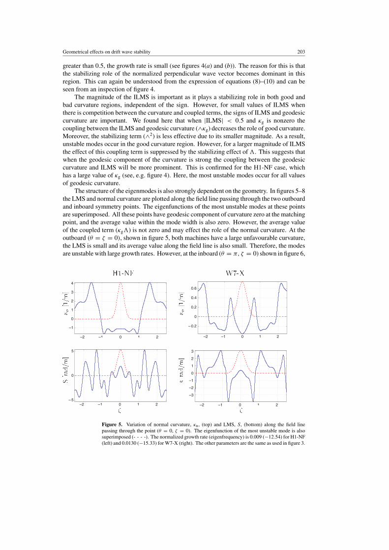
The structure of the eigenmodes is also strongly dependent on the geometry. In figures 5–8the LMS and normal curvature are plotted along the field line passing through the two outboardand inboard symmetry points. The eigenfunctions of the most unstable modes at these pointsare superimposed. All these points have geodesic component of curvature zero at the matchingpoint, and the average value within the mode width is also zero. However, the average valueof the coupled term (κg�) is not zero and may effect the role of the normal curvature. At theoutboard (θ = ζ = 0), shown in figure 5, both machines have a large unfavourable curvature,the LMS is small and its average value along the field line is also small. Therefore, the modesare unstable with large growth rates. However, at the inboard (θ = π, ζ = 0) shown in figure 6,

–2 –1 0 1 2 –2 0 1 2

–2 –1 0 1 2 –2 0 1 2

– 0.2

0

0.2

0.4

0.6

–1

–1

0

1

2

3

4

–1

0

5

– 5

–2

0

1

2

3

–1

–3

Figure 5. Variation of normal curvature, κn, (top) and LMS, S, (bottom) along the field linepassing through the point (θ = 0, ζ = 0). The eigenfunction of the most unstable mode is alsosuperimposed (- - - -). The normalized growth rate (eigenfrequency) is 0.009 (−12.54) for H1-NF(left) and 0.0130 (−15.33) for W7-X (right). The other parameters are the same as used in figure 3.

204 M H Nasim et al

–2 –1 0 1 2 – 2 –1 0 1 2

– 2 –1 0 1 2 –2 –1 0 1 2

–1

– 0.5

0

0.5

1

1.5

2

2.5

3

– 0.2

0

0.2

0.4

0.6

– 8

– 6

– 4

– 2

0

2

4

0

1

2

3

4

5

– 3

– 2

–1

Figure 6. Same as figure 6, except for the line passing through the point (θ = π , ζ = 0),and the normalized growth rate (eigenfrequency) is 0.0083 (−13.23) for H1-NF (left) and 0.0137(−16.85) for W7-X (right). Note that the eigenfrequencies are Doppler shifted to higher valuesthan the modes at (θ = 0, ζ = 0).

–1 0 1 2 3

–1

–0.5

0

0.5

1

1.5

2

2.5

–1 0 1 2 3

–0.2

0

0.2

0.4

0.6

–2 –1 0 1 2 3 4

–8

–6

–4

–2

0

2

4

–4

–3

–2

–1

0

1

2

3

4

–2 –1 0 1 2 3 4

Figure 7. Same as figure 6, except for the line passing through the point (θ = 0, ζ = π/N ),and the normalized growth rate (eigenfrequency) is 0.0115 (−14.56) for H1-NF (left) and 0.0011(−4.29) for W7-X (right), where N is the field period.

both machines have favourable curvature but have low average values of LMS within the modewidth and hence small ILMS value. This implies that there is only a small stabilizing effect ofb due to its small value. Consequently the growth rate is relatively small compared with theprevious case. The geodesic curvature plays no role at this point due to the vanishing of �.

Geometrical effects on drift wave stability 205

–1 0 1 2 3

–1 0 1 2 3

–1

0

1

2

3

4

–1 0 1 2 3

– 0.2

0

0.2

0.4

0.6

–3

–2

–1

0

1

2

3

4

5

–1 0 1 2 3–8

–6

–4

–2

0

2

4

Figure 8. Same as figure 6, except for the line passing through the point (θ = π , ζ = π/N ),and the normalized growth rate (eigenfrequency) is 0.0057 (−10.18) for H1-NF (left) and 0.0027(−7.16) for W7-X (right).

However, a very small shift from the symmetry point, achieved by selecting an other field line,increases the growth rate. Now the small magnitude of ILMS coupled with κg increases theinstability, which can again be understood in terms of equations (8)–(10).

At the second outboard symmetry point (θ = 0, ζ = π/N ), shown in figure 7, H1-NF hasa more favourable curvature compared with the point at (θ = π , ζ = 0). The average valueof LMS within the mode extent is small positive at (θ = 0, ζ = π/N ), compared with smallnegative at (θ = π, ζ = 0). Both regions are unstable since there is only a small stabilizingeffect of b. However, the role of the good curvature is suppressed due to coupling betweenthe geodesic curvature and ILMS, in the former case resulting in a higher growth rate. On theother hand, for W7-X, the curvature is not favourable but the magnitude of the growth rateis still smaller than the point (θ = π, ζ = 0), where the curvature is large and favourable.This is due to the large value of LMS within the mode extension. Figure 8 shows the point(θ = π, ζ = π/N), where both stellarator configurations have unfavourable curvature, a smallvalue of ILMS and smaller growth rates than at (θ = 0, ζ = 0), shown in figure 5. The smallervalue of growth rate is due to the less unfavourable curvature and relatively large values ofILMS. The role of unfavourable curvature is suppressed in W7-X, while it is enhanced inH1-NF, due to the coupling between κg and ILMS. At this point this results in smaller growthrates in W7-X.

Drift waves have been considerably more studied in tokamaks than in stellarators. Asa reference, these results are compared with a tokamak having an aspect ratio comparablewith W7-X. The normalized growth rate, γ , b = (B0/Bχ |k⊥|)2 and the curvature and ∇B

drift frequency, �d and |B|, along θ0[rad] with ζ0 = 0 on the magnetic surface s = 34 for

a circular cross section tokamak (left), for H1-NF (middle) and for W7-X (right) are shownin figure 9. The variation of geodesic curvature, κg, ILMS along the field line �, normalcurvature, κn, and LMS are also shown for these configurations. The other parameters are thesame as used in figure 3. The highest growth rate for the tokamak is found at the outboard(θ = 0 = ζ ) where the curvature is unfavourable and the stabilizing b and LMS are small,

206 M H Nasim et al

Figure 9. The normalized growth rate, γ , the curvature and ∇B drift frequency, �d,b = ((B0/B)χ |k⊥|ζ=ζ0

)2, normal curvature, κn, geodesic curvature, κg, ILMS along the field

line �, LMS and |B| along θ0[rad] with ζ0 = 0 on the magnetic surface s = 34 for circular tokamak

(left), for H1-NF (middle) and for W7-X (right). The other parameters are the same as used infigure 3.

Geometrical effects on drift wave stability 207

and the minimum growth rate is found at the inboard (θ = π , ζ = 0) where the curvatureis favourable and the stabilizing b and LMS are large. These are the well-known results. Itis interesting to mention here that the coupling of geodesic curvature and ILMS enhances thecurvature effect in a tokamak, increasing stability at a good curvature and decreasing stabilitywhere the curvature is bad. Hence, in tokamaks the effect of curvature is dominating. On theother hand, for stellarators, large values of growth rate are found not only at the outboard butalso at the inboard where b as well as � have minimum values. A strong correlation betweenthe growth rate and b as well as with � can be seen. In addition the rather large fluctuationsin the growth rates observed for both stellarators are due to the fluctuations in �d. Thesefluctuations may arise due to the coupling effect of κg and ILMS. However, the effect is notstrong in tokamaks, at least not at a large aspect ratio. However, for H1-NF at the inboard,LMS is large and positive, but its integrated value along the field line is zero, and so this regionis unstable either due to large positive LMS or due to vanishing of ILMS.

The frequency and growth rate of the most unstable modes are well correlated with ILMSfor both stellarators, but their dependence on LMS is qualitatively different, W7-X having astronger correlation with LMS. This is because in W7-X the LMS and ILMS coincide andchange periodically in the same way, which they do not in H1-NF. It is interesting to notethat Jost [34] did not find any dependence of drift wave instability on the LMS by usingglobal calculations in a quasi-symmetric configuration, suggesting that for a stellarator thegrowth rates correlate stronger with ILMS than with LMS. For some configurations suchas W7-X the variation of LMS and ILMS coincide, while for others, like H1-NF, theydo not.

5. Summary

In this paper we have reported the geometrical effects on the stability of the universal driftwave. The role of LMS, ILMS along the field line and curvature have been discussed using twodifferent stellarators, and a circular tokamak is used as a reference. It has been demonstratedthat the main features of the variation of stability can be understood in terms of the variationof the equilibrium quantities.

In the stellarators the most unstable localized modes along the field line are found in bothgood and bad curvature regions, while in tokamaks, these are found only in the bad curvatureregion. The existence of these modes in the good curvature region in stellarators is due tothe effect of strong coupling between geodesic curvature and ILMS. This coupling suppressesthe effect of good curvature and modifies the point at which the curvature drive is maximum.This coupling is stronger in H1-NF than in W7-X due to the larger magnitude of the geodesiccurvature. However, in the large aspect ratio tokamak, this coupling increases stability in goodcurvature regions and decreases stability in bad curvature regions.

The eigenfunctions have a finite width along the field lines. They are more localized inbad curvature regions and more extended in good curvature regions, and whenever there is arapid change in the local values of equilibrium quantities within the mode width, the mode willbe more influenced by the averaged values rather than by the local values. The most unstablemodes are either symmetric or asymmetric, depending on the position on the magnetic surface.These modes are highly localized and have the largest frequencies.

In this paper we have also demonstrated that the role of the LMS on the stability of lineardrift waves is qualitatively different for different stellarators. In W7-X, the growth rate dependsessentially upon the magnitude of the LMS, while in H1-NF, it is also sensitive to the sign.We have also shown that the role of the LMS on the growth rates and frequencies can be bestunderstood in terms of its integrated value along the field line.

208 M H Nasim et al

The magnitude of the ILMS plays a stabilizing role both in good and bad curvature regions.The sign of the ILMS along the field line is also important. When it is small the coupling withgeodesic curvature modifies the curvature drive. However, for larger values of ILMS thestabilizing role dominates the small shift in the curvature drive.

This work has implications on optimization of stellarator design specifically with respectto minimization of drift wave turbulence, while this is a considerable challenge that will requireconsiderable work in the future. The following conclusions can be drawn from this study. Themodes considered are more dependent on the ILMS than the curvature. For a sufficientlylarge ILMS, it dominates the effect of curvature and can be stabilized by the drift modes,regardless of the value of curvatures. This suggests that maximizing the ILMS value in astellarator configuration is an important optimization criterion in stellarator design. Generally,a large LMS is beneficial to ideal MHD, while neoclassical transport depends primarily uponthe details of |B|. Therefore, ILMS has no direct negative effects on neoclassical transport.An increase in the LMS in some regions could be obtained by enhancing shaping effects likeelongation and triangularity [35]. This, however, clearly also changes the curvature of the fieldlines and can also change the |B| spectrum. Thus, when the magnetic field is optimized withrespect to drift wave stability, the new configuration needs to be checked and evaluated withrespect to other properties. An optimization procedure like the one described can be expectedto be very complex and computer intensive and is therefore a considerable challenge. It shouldbe noted that ITG modes and other modes that are driven primarily by the curvature are not asstrongly affected by the ILMS.

The main limitations of this investigation are the ad hoc use of the driving mechanismand the use of the ballooning mode formalism. The driving mechanism appears in our driftwave equation through the δ, which is kept constant in this study. In a more realistic model, δ

should depend both on geometry and physics. This would change the spectrum of the modesin particular in the favourable curvature region, but it will also complicate the interpretation ofthe results presented. Furthermore, instead of solving the drift wave equation along the fieldline using ballooning mode formalism, more realistically one could solve the wave equationsimultaneously in radial and parallel directions. This was done by Kleiber [17], and he foundsome extra modes for negative magnetic shear with growth rates that are greater than thoseobtained using ballooning mode formalism. Alternatively, the local structure should be coupledto a ray tracing algorithm, as was done by Dewar and Glasser [29], or to a surface constructionalgorithm like that used by Cooper et al [36]. However, this study has given a good indicationof localization and the stability of drift waves in a stellarator geometry. In the future we willextend this study to include more complete physics.

Acknowledgment

Discussions with Dr M Nadeem are gratefully acknowledged. This work was supported byfunding from the Euratom/VR Association.

References

[1] Nuhrenberg J and Zille R 1987 Theory of Fusion Plasmas ed A Bondeson et al (Verenna: Editrice CompositoriBologna) p 3

[2] Lyon J F et al 2002 13th International Stellarator Workshop (Canberra, Australia, 25 February–March 2002)Paper No OV.1

[3] Tang W M 1978 Nucl. Fusion 18 1089[4] Boozer A H 1990 Phys. Fluids B 2 2870[5] Tang W M, Rewoldt G and Chen L 1986 Phys. Fluids 29 3715

Geometrical effects on drift wave stability 209

[6] Redd A J, Hritz A H, Batman G, Rewoldt G and Tang W M 1999 Phys. Plasmas 6 1162[7] Dominguez N, Carreras B A, Lynch V E and Diamond P H 1992 Phys. Fluids B 4 2894[8] Horton W 1999 Rev. Mod. Phys. 71 735[9] Rewoldt G, Ku L P, Tang W M, Sugama H, Nakajima N, Watanabe K Y, Murakami S, Yamada H and Cooper W A

2000 Phys. Plasmas 7 4942[10] Waltz R E and Boozer A H 1993 Phys. Fluids B 5 2201[11] Green J M and Chance M S 1981 Nucl. Fusion 21 453[12] Dewar R L, Monticell D A and Sy W N-C 1984 Phys. Fluids 27 1723[13] Lewandowski J L V and Persson M 1995 Plasma Phys. Control. Fusion 37 1199[14] Persson M, Lewandowski J L V and Nordman H 1996 Phys. Plasmas 3 3720[15] Persson M, Nadeem M, Lewandowski J L V and Gardner H J 2000 Plasma Phys. Control. Fusion 42 203[16] Uddholm P, Nadeem M and Persson M 2000 Plasma Phys. Control. Fusion 42 501[17] Kleiber R 2001 Phys. Plasmas 9 4090[18] Greene J M and Johnson J L 1968 Plasma Phys. 10 729[19] Hegna C C and Nakajima N 1998 Phys. Plasmas 5 1336[20] Lewandowski J L V 1998 Plasma Phys. Control. Fusion 40 283[21] Kendl A and Wobig H 1999 Phys. Plasmas 6 4714[22] Renner H, W7AS Team, NBI Group and ECRH Group 1989 Plasma Phys. Control. Fusion 31 1579[23] Grieger G et al 1991 Plasma Phys. Control. Fusion Research 1990 vol 3 (Vienna: International Atomic Energy

Agency) p 525[24] Wobig W 1993 Plasma Phys. Control. Fusion 35 903[25] Hamberger S M, Blackwell B D, Sharp L E and Singleton B D 1990 Fusion Technol. 17 123[26] Hirshman S P and Betancourt O 1991 J. Comput. Phys. 96 99[27] Connor J W and Taylor J B 1987 Phys. Fluids 30 3180[28] Koch R R and Horton W 1975 Phys. Fluids 18 861[29] Dewar R L and Glasser A H 1983 Phys. Fluids 26 3038[30] Nadeem M, Rafiq T and Persson M 2001 Phys. Plasmas 8 4375[31] Dewar R L and Hudson S R 1998 Physica D 112 275[32] Horton W Jr, Estes R, Kwak H and Duk-in Choi 1978 Phys. Fluids 21 1366[33] Rafiq T, Kleiber R, Nadeem M and Persson M 2002 Phys. Plasmas 9 4929[34] Jost G, Tran T M, Cooper W A, Villard L and Appert K 2001 Phys. Plasmas 7 3221[35] Kendl A and Wobig H 2000 27th EPS Conf. on Control. Fusion and Plasma Phys. (Budapest, Hungary,

12–16 June 2000) vol 24B (ECA) p 992[36] Cooper W A, Singleton D B and Dewar R L 1996 Phys. Plasmas 3 1162