P O S I V A O Y

O l k i l u o t o

F I -27160 EURAJOKI , F INLAND

Te l +358-2-8372 31

Fax +358-2-8372 3709

Alvaro Buoro

K im Dah lbo , Laur i W i ren

Johan Ho lmén , Jan Hermanson

Aaron Fox (ed i to r )

October 2009

Work ing Repor t 2009 -77

Geological Discrete-Fracture Network Model(version 1) for the Olkiluoto Site, Finland

October 2009

Base maps: ©National Land Survey, permission 41/MML/09

Working Reports contain information on work in progress

or pending completion.

The conclusions and viewpoints presented in the report

are those of author(s) and do not necessarily

coincide with those of Posiva.

Alvaro Buoro ,

K im Dah lbo , Laur i Wi ren

Golde r Assoc ia tes Oy

Johan Ho lmén , Jan Hermanson ,

Aaron Fox (ed i to r )

Golde r Assoc ia tes AB

Work ing Report 2009 -77

Geological Discrete-Fracture Network Model(version 1) for the Olkiluoto Site, Finland

Geological Discrete-Fracture Network Model (version 1) for the Olkiluoto Site, Finland ABSTRACT This report describes the methods, analyses, and conclusions of the modelling team in

the production of a discrete-fracture network (DFN) model for the Olkiluoto Site in

Finland. The geological DFN is a statistical model for stochastically simulating rock

fractures and minor faults at a scale ranging from approximately 0.05 m to

approximately 500 m; an upper scale limit is not expressly defined, but the DFN model

explicitly excludes structures at deformation-zone scales (~ 500 m) and larger. The

DFN model is presented as a series of tables summarizing probability distributions for

several parameters necessary for fracture modelling: fracture orientation, fracture size,

fracture intensity, and associated spatial constraints.

The geological DFN is built from data collected during site characterization (SC)

activities at Olkiluoto, which is currently planned to function as a final deep geological

repository for spent fuel and nuclear waste from the Finnish nuclear power program.

Data used in the DFN analyses include fracture maps from surface outcrops and

trenches (as of July 2007), geological and structural data from cored boreholes (as of

July 2007), and fracture information collected during the construction of the main

tunnels and shafts at the ONKALO laboratory (January 2008).

The modelling results suggest that the rock volume at Olkiluoto surrounding the

ONKALO tunnel can be separated into three distinct volumes (fracture domains): an

upper block, an intermediate block, and a lower block. The three fracture domains are

bounded horizontally and vertically by large deformation zones. Fracture properties,

such as fracture orientation and relative orientation set intensity, vary between fracture

domains.

The rock volume at Olkiluoto is dominated by three distinct fracture sets:

subhorizontally-dipping fractures striking north-northeast and dipping to the east, a

subvertically-dipping fracture set striking roughly north-south, and a subvertically-

dipping fracture set striking approximately east-west. The subhorizontally-dipping

fractures account for most (55% - 60%, depending on fracture domain) of the total

observed fracture intensity at Olkiluoto. Fracture intensity shows a correlation with

depth below the ground surface, with exponential functions used to describe the change

in volumetric fracture intensity (P32) with depth. Fracture intensity is greatest within the

intermediate fracture domain and least in the lower fracture domain.

Three alternative DFN models are presented, based on different weightings of the

importance of individual datasets. In Case 1, the fracture orientation and intensity

models are based solely on borehole data; this case is focused on correctly modelling

intensity in the upper fracture domain. Case 2 is focused on producing a better match

between simulated and observed fracture trace maps at surface outcrops. Finally in Case

3, the size model is modified so as to give greater weight to fracture traces observed in

the ONKALO tunnel. Together, these three models provide an initial estimate of

variability in geological DFN parameters.

Keywords: fractures, deformation zone, fracture domain, orientation, size, intensity,

ONKALO, Olkiluoto, DFN, stochastic.

Olkiluodon Geologinen DFN-malli (versio 1) TIIVISTELMÄ Tässä raportissa esitetään Olkiluodon tutkimusalueen geologisessa DFN-mallinnuksessa

(diskreetti rakoverkkomallinnus) käytetyt menetelmät ja tehdyt analyysit ja johto-

päätökset. Geologinen DFN on tilastollinen malli jolla voidaan stokastisesti simuloida

kooltaan noin viidestä senttimetristä noin 500 metriin vaihtelevien rakojen ja pienten

siirrosvyöhykkeiden esiintymistä kalliossa. DFN-malli esitetään taulukkoina, joihin on

koottu tiedot jakaumista eri parametreille: rakojen suunta, rakojen koko, rakotiheys ja

rakojen paikkaa koskevat ehdot.

Geologinen DFN perustuu Olkiluodon paikkatutkimusaineistoon. Aineisto on kerätty

tutkimusalueelta, johon ollaan tekemässä loppusijoituslaitosta Suomen käytetylle

ydinpolttoaineelle. DFN-mallinnuksessa käytetty data sisältää kesällä 2007 käytössä

olleet tutkimuskaivantojen ja paljastumien rakokartat sekä kairasydämistä kartoitetut

geologiset tiedot. Työssä on myös käytetty vuoden 2008 alussa käytössä ollutta

rakoaineistoa ONKALO-tutkimustunnelista.

Mallinnuksen tulosten mukaan näyttää siltä, että ONKALOn alueen kallio voidaan

jakaa kolmeen erilliseen rakoilutilavuuteen: ylempään, keskimmäiseen ja alempaan

blokkiin. Näitä tilavuuksia rajaavat suuret deformaatiovyöhykkeet. Rakoilun ominai-

suudet, kuten suunta ja rakosettien suhteelliset intensiteetit, vaihtelevat näiden tilavuuk-

sien välillä.

Olkiluodon kalliossa vallitsee kolme rakosettiä: loivat kaateen suunnaltaan itäkaakkoon

olevat sekä pohjois-eteläsuuntaiset ja itä-länsisuuntaiset melkein pystyt setit. Loivat raot

käsittävät rakoilutilavuudesta riippuen 55–60 % kaikista raoista. Rakotiheys näyttää

riippuvan syvyydestä. Muutosta tilavuudellisessa rakotiheydessä (P32) voidaankin

syvyyden suhteen kuvata eksponenttifunktioilla. Rakotiheys on suurin keskimmäisessä

rakoilutilavuudessa ja pienin alemmassa

Raportissa esitetään kolme vaihtoehtoista DFN-mallia, jotka perustuvat datasettien

erilaisiin painotuksiin. Vaihtoehdossa 1 rakojen suunta- ja tiheysmallit perustuvat pel-

kästään kairareikäaineistoon. Tällä vaihtoehdolla voidaan parhaiten mallintaa ylemmän

rakoilutilavuuden rakoilua. Vaihtoehto 2 on tehty sopimaan paremmin yhteen kaivan-

tojen ja paljastumien rakokarttojen kanssa. Vaihtoehdossa 3 rakojen kokojakauman

luomisessa on painotettu eniten tunnelista tehtyjä rakokarttoja. Näiden kolmen mallin

avulla voidaan arvioida DFN-parametrien vaihtelua Olkiluodon kalliossa.

Avainsanat: rako, deformaatiovyöhyke, rakoilutilavuudet, suunta, koko, intensiteetti,

ONKALO, Olkiluoto, DFN, stokastinen.

1

TABLE OF CONTENTS ABSTRACT TIIVISTELMÄ

1 INTRODUCTION................................................................................................... 3

1.1 Introduction and purpose of study ................................................................... 3 1.2 Model volume, use, and applicability ............................................................... 3 1.3 DFN terminology and acronyms ...................................................................... 4 1.4 Data and software used .................................................................................. 6

2 DFN MODEL METHODOLOGY .......................................................................... 13

2.1 Modelling strategy and assumptions ............................................................. 13 2.1.1 Geological DFN model strategy and base methodology ......................... 13 2.1.2 Geological DFN model assumptions....................................................... 15

2.2 Fracture domains .......................................................................................... 16 2.3 Fracture orientation ....................................................................................... 18

2.3.1 Geological coordinates and the orientation of fractures in space ............ 18 2.3.2 Spherical projections and the univariate Fisher distribution .................... 19 2.3.3 Terzaghi correction ................................................................................. 21 2.3.4 Classification of observed fractures into fracture sets ............................. 23 2.3.5 Concentrations of fracture poles – clusters and girdles........................... 24

2.4 Fracture size ................................................................................................. 25 2.4.1 Fracture size as a power law .................................................................. 27 2.4.2 Estimating power law distribution parameters using FracSize ................ 28 2.4.3 Trace length scaling exponent analysis as a verification of ........................ FracSize-derived models ........................................................................ 30

2.5 Fracture intensity ........................................................................................... 33 2.5.1 Calculating P32 from Terzaghi-compensated P10 (P10Te) .......................... 34 2.5.2 Analysis of fracture intensity ................................................................... 36 2.5.3 Calibration of the coupled size-intensity model ....................................... 37

2.6 Fracture spatial (location) model ................................................................... 39 2.6.1 Fracture size / intensity scaling model .................................................... 40 2.6.2 Depth-dependence of fracture intensity .................................................. 43 2.6.3 Fracture termination relationships .......................................................... 43

3 DERIVATION OF THE OLKILUOTO GEOLOGICAL DFN ................................... 45

3.1 Identification of fracture domains ................................................................... 45 3.2 Fracture orientation model ............................................................................ 47

3.2.1 Orientation model alternatives ................................................................ 48 3.2.2 Case 1: All fractures in all boreholes ...................................................... 52 3.2.3 Case 2: fracture orientation correlated to bedrock lithology .................... 57 3.2.4 Case 3: fracture orientation as a function of depth .................................. 60 3.2.5 Case 4: fracture orientation as a function of fracture domain .................. 64 3.2.6 Fracture orientation model ...................................................................... 74 3.2.7 Orientation model applied to trenches, outcrops, and the ONKALO .......... tunnel ..................................................................................................... 75

3.3 Fracture intensity model ................................................................................ 80 3.3.1 Model Implementation ............................................................................ 80 3.3.2 Fracture intensity in selected boreholes as function of depth .................. 83 3.3.3 Fracture intensity as a function of depth interval, lithology or fracture ........

2

domain ................................................................................................... 90 3.3.4 Fracture intensity as a function of depth and fracture domain ................. 97 3.3.5 Fracture intensity outside fracture domains .......................................... 103 3.3.6 Fracture intensity at trenches and outcrops .......................................... 103 3.3.7 Fracture intensity in the ONKALO tunnel .............................................. 105 3.3.8 Fracture intensity model ....................................................................... 105

3.4 Fracture size model ..................................................................................... 106 3.4.1 Model implementation .......................................................................... 106 3.4.2 FracSize analysis results ...................................................................... 108 3.4.3 Tracelength scaling analysis on surface outcrops ................................. 118

3.5 Fracture spatial model ................................................................................. 120 4 MODEL CALIBRATION AND VERIFICATION .................................................. 127

4.1 Calibration strategy ..................................................................................... 127 4.2 Outcrop simulations .................................................................................... 128 4.3 ONKALO tunnel simulations ........................................................................ 137 4.4 Borehole simulations ................................................................................... 143 4.5 Calibration results and recommendations.................................................... 145

5 CONCLUSIONS AND RECOMMENDATIONS .................................................. 147

5.1 Version 1.0 DFN model summary ............................................................... 147 5.2 DFN model uncertainties ............................................................................. 149 5.3 Conclusions and recommendations for future work ..................................... 151

REFERENCES ......................................................................................................... 153

3

1 INTRODUCTION

1.1 Introduction and purpose of study

The intended use of the geological discrete fracture network (Geo-DFN) model is as

input for hydrogeological and mechanical modelling, and to condense fracture-related

data into a form that is accessible for planning, site engineering and repository safety

assessment. The DFN model is presented as a mathematical description of the fracturing

and not as a static model. As such, the model parameters can be implemented in

different forms as necessary by the downstream users of the Geo-DFN description. DFN

parameters can be used as input to discrete element modelling codes such as FLAC or

3DEC, or can be upscaled to finite-difference grid volumes of various sizes for use in

continuum modelling (groundwater, contaminant transport).

This report documents the first attempt (version 1.0) at a site-scale geological DFN

model at Olkiluoto. The geological DFN discussed in this report represents a stochastic

description of fracturing within the rock mass at Olkiluoto; the ranges of variation of the

derived DFN-properties are the product of both the natural heterogeneity of the studied

system and the uncertainty in the available input data. Though the boundaries of the

fracture domains (c.f. Section 2.2) are explicitly specified, the locations and sizes of

individual fractures inside the domains are not pre-ordained. Instead, fracture geometric

properties are delivered as probability distributions, with associated limits and

recommended values.

The DFN model has been simplified through the use of global orientation models and a

consistent methodology for describing fracture size and intensity through the use of

power laws. To build confidence in the DFN model parameterisations, a series of

verification cases using outcrop and borehole fracture data were performed. The

verification cases illustrate the limits of applicability of the DFN model

parameterization and provide a snapshot of the reproductive capability of the model.

1.2 Model volume, use, and applicability

This geological DFN model describes rock fracturing within a volume proposed for use

as a spent fuel repository for the Finnish commercial power generation program. The

proposed repository is located on the island of Olkiluoto, which lies along the Baltic Sea

on Finland‟s western coast. In 1999 Posiva Oy selected the bedrock of the Olkiluoto

peninsula in Eurajoki municipality as a suitable area for the final repository. Approval

for site investigations was granted by the Finnish Parliament in 2001. Construction of

an underground research facility at Olkiluoto (called ONKALO) started in 2004. The

geological DFN model is built atop site-characterization efforts as well as investigations

made in support of the ONKALO laboratory.

The DFN model is only applicable within the fracture domains specified in this report

(Section 3.1) inside the Olkiluoto local model volume. Applicability outside these limits

has not been established nor tested, and users who wish to use the model outside the

range of applicability should carefully evaluate the parameters and limitations of the

Olkiluoto geological DFN prior to using the model outside the context for which it was

constructed. The DFN model is based upon the source data and software described in

4

Section 1.4 and the assumptions listed in Section 2.1.2. Any future data additions or

revisions, new conceptual understandings, or changes in assumptions or definitions

could require the presented model to be revised.

Figure 1-1. Geological map of Olkiluoto site, indicating the location of the local and

regional model volumes and major regional lineament traces. Map is cast in Zone 1 of

the Finnish KKJ national grid system. The inset map illustrates the location of Olkiluoto

relative to the rest of Finland and northern Europe.

1.3 DFN terminology and acronyms

CDF - Cumulative Density Function: A function that quantifies the cumulative

probability of a distribution. The term is used in this report in the description of fracture

trace length and radius distributions. It is the probability that the value of a randomly

selected value is less than a specified value.

CCDF – Complementary Cumulative Density Function: A function that quantifies

the cumulative probability of a distribution. The term is used in this report in the

description of trace length and radius distributions. It is the probability that the value of

a randomly selected value is greater than a specified value. The CCDF is equal to 1

minus the CDF.

CCN – Complementary Cumulative Number: A type of plot in which the number of

data values greater than or equal to a specific value are plotted as a function of the

5

value. CCN plots are used in this report for estimating the size model for the Tectonic

Continuum alternative model.

CFI – Cumulative Fracture Intensity: A type of plot used to identify fractured zones

and quantify their characteristic fracture intensity. The CFI utilizes the cumulative

number of fractures, plotted as a CDF versus depth or elevation. Changes in fracture

intensity are marked by abrupt changes in the slope of the curve, while straight

segments illustrate sections where fracture intensity is relatively constant with depth.

DFN – Discrete Fracture Network model: A three-dimensional numerical model in

which fractures are represented as finite surfaces with specified mechanical and

hydraulic properties.

DZ – Deformation Zone: This notation is employed as a general description of a zone

characterised by ductile or brittle deformation, or a combination of the two. Generally,

deformation zones are deterministic structures in site geological models, and are

therefore characterized separately from the DFN.

Euclidean Scaling, Euclidean Dimension: A scaling behaviour characterised by a

first-order relation between the number or density of some object, and the extent of the

space in which it is embedded. In this report it is used to describe fracture intensity; a

Euclidean scaling model for fracture intensity would be characterised by a linear, first

order relation between the number of fractures in a volume of rock and the volume

itself. Doubling the volume would lead to a doubling of the number of fractures in a

Euclidean scaling model. The Euclidean dimension is a fractal mass dimension that

characterises Euclidean scaling. It is 1.0 for line samples, such as borehole fracture

data, 2.0 for areal samples, such as outcrop fracture trace data, and 3.0 for volumetric

samples, such as rock volumes.

Fracture Domain: A fracture domain refers to a rock volume outside deformation

zones in which rock units show similar fracture characteristics, such that the variability

between domains is (ideally) larger than the variability within a single domain. In this

version of the Olkiluoto geological DFN, the boundaries of the fracture domains are

defined in terms of large regional subhorizontally-dipping deformation zones. The

zones differ predominantly in terms of their relative fracture set intensities and in the

location of the orientation set mean poles.

Mass Dimension: A measure of the scaling behaviour of a group of objects. In this

report, the mass dimension is used to quantify the scaling behaviour of fracture intensity

in boreholes and outcrops.

Mechanical Stratigraphy: The subdivision of the rock mass into discrete intervals,

based largely on the rheology and deformation behaviour of the intervals. Mechanical

stratigraphy may cut across multiple lithostratigraphic intervals.

P10 – A measure of linear fracture intensity, expressed in this report as the number of

fractures per meter (1/m). P10 is generally recorded in boreholes or along scanlines.

6

P10Te – Terzaghi-compensated P10. This is a composite measurement that partially

accounts for the orientation bias caused by line sampling of a network of planar

features. P10Te is not the same thing as P32; however, it can be viewed as an initial

estimate of P32. See Section 2.5.1 for more details.

P21 – A measure of areal fracture density, expressed in this report as the fracture trace

length per unit of mapped area (m/m2). P21 is generally recorded on surface outcrops or

tunnel walls.

P32 – A measure of volumetric fracture intensity, expressed in this report as fracture

surface area per unit of rock volume (m2/m

3). It is very difficult to measure P32 in the

field; it is generally either calculated from other intensity measurements (P10, P21)

through stochastic simulation or estimated analytically (Wang, 2005; Terzaghi, 1965)

Statistical Significance – This relates to the outcome of a statistical test of a

hypothesis. It is the probability of the results of the statistical tests given that the

hypothesis is true with reference to a specified value of probability for which the

hypothesis is rejected or not rejected. The test of statistical significance does not prove

that the hypothesis is true, but rather that the data do or do not reach the probability

level of falsifying the hypothesis. Statistical significance is quantified as the parameter

α, which represents the probability that the null hypothesis for the statistical test being

performed will be rejected when it is in fact true (a Type I error). In general, an α of

0.05 has been used as a level of significance in the geological DFN modelling.

1.4 Data and software used

DFN modelling relies primarily on geometric information about fractures recorded in

cored boreholes, from fracture traces on tunnel walls and surface outcrops, from

lineament maps constructed using regional geological and geophysical mapping, and, if

available, seismic data. The data analyzed in the production of the version 1.0

geological DFN model is taken from the Site Characterization database for the

Olkiluoto site. This study utilizes cored borehole, surface trench, and surface outcrop

data up to a cut-off date of July 2007 („data freeze‟). In addition, a database of fractures

recorded along sections of the ONKALO tunnel through January of 2008 is also used.

A total of 58 boreholes are used in the development of the geological DFN model, with

a total of 33,457 recorded fractures suitable for inclusion in the data analysis. A fracture

is deemed suitable for inclusion in the borehole database if it has a defined orientation

(strike, dip or dip, dip direction) and is not within the limits of a structure modelled in

the deformation zone model. A brief summary of the borehole data is presented in

Table 1-1.

Two-dimensional fracture data, including orientations and fracture trace lengths, was

obtained from two roughly rectangular outcrops (OL-TK10 and OL-TK11) that were

mapped in detail for fracturing and 11 trenches (OL-TK1 through OL-TK13). Scanline

data along 13 additional narrow surface trenches was made available to the DFN team,

but is not utilized in this model version due to perceived data quality and sampling bias

issues. In addition, 3,451 fractures over an approximately 1800 m long section of the

7

ONKALO tunnel were utilized for fracture orientation and size parameterization. The

trace maps began at a length (chainage) of 300 m along the ONKALO tunnel, and

extend to a total length of 2100 m. A brief summary of the recorded fracture trace data

is presented in Table 1-2.

A number of large deformation zones have been identified in the area and studied by

Posiva (see Olkiluoto Geological report version 1, Paulamäki et al 2007). It is important

to note that the DFN model is described solely for volumes of rock outside of

deformation zones. As such, where possible, fractures inside deformation zone cores

were excluded from all analyses. The borehole database provided by Posiva defines

only fractures lying inside the core of a deformation zones and not the so-called

„transition zone‟ (c.f. Figure 3-95 and Figure 5-1, Wahlgren et al. 2008, after Caine et

al., 1996) surrounding the core of the deformation zone. Future work may focus on the

identification of these „transition zones‟ in the cored borehole data set. According to

Posiva the deformation zones of most importance at Olkiluoto are: OL-BFZ002, OL-

BFZ055, OL-BFZ018, OL-BFZ055, OL-BFZ056, OL-BFZ080, and OL-BFZ098.

Figure 1-3 and Figure 1-2 illustrate the spatial locations of the primary data sources for

the version 1.0 Olkiluoto geological DFN model.

Figure 1-2. 3D isometric view of the DFN model domain (blue), the ONLKALO tunnel

(purple), cored borehole array (white), and Olkiluoto Island (transparent green). Note

that some well name labels have been omitted for visual clarity.

Figure 1-3. Locations of core-drilled boreholes, detail-mapped fracture outcrops, and the ONKALO tunnel, along the walls of which

detailed fracture trace mapping was performed.

8

9

Table 1-1. Available data in cored boreholes at Olkiluoto.

Borehole Number of fractures

Number of fractures with

complete orientation data

Borehole Length (m)

KR1 2136 1837 1000.7

KR2 2715 2031 1051.9

KR3 1363 942 502.0

KR4 1486 0 901.4

KR5 1306 1075 554.0

KR6 1535 1286 600.6

KR7 1549 867 810.6

KR8 1430 1162 600.5

KR9 1254 1082 599.2

KR10 815 625 612.7

KR11 1399 986 1001.9

KR12 2677 2210 795.3

KR13 1867 1702 500.0

KR14 786 637 513.3

KR15 603 524 517.7

KR16 339 282 169.7

KR17 257 230 156.6

KR18 140 112 125.3

KR19 1669 1530 536.2

KR20 988 954 494.4

KR21 1131 962 301.0

KR22 1763 1559 499.1

KR23 582 531 295.2

KR24 898 619 549.6

KR25 1368 1257 604.9

KR26 384 273 102.7

KR27 1616 1418 549.5

KR28 954 637 656.2

KR29 1267 901 866.2

KR30 238 211 98.2

KR31 521 398 334.4

KR32 649 534 191.8

KR33 699 649 309.7

KR34 349 331 99.2

KR35 325 274 100.8

KR36 497 343 204.9

KR37 558 494 345.3

KR38 798 686 523.0

KR39 788 0 497.9

KR40 1698 0 1029.8

KR15B 142 118 45.0

KR16B 96 72 44.8

KR17B 98 78 45.3

10

Borehole Number of fractures

Number of fractures with

complete orientation data

Borehole Length (m)

KR18B 153 114 45.2

KR19B 184 141 45.0

KR20B 261 160 45.1

KR22B 202 106 45.4

KR23B 157 135 45.1

KR25B 124 99 44.9

KR27B 123 91 44.9

KR27B 123 91 44.9

KR28B 98 82 44.9

KR29B 146 127 45.6

KR31B 121 110 44.9

KR33B 134 117 44.6

KR37B 188 178 45.0

KR39B 157 0 44.6

KR40B 118 0 44.6

Table 1-2. Descriptive statistics of fracture traces recorded on outcrops and tunnel

walls longer at Olkiluoto.

Outcrop / Tunnel

Segment

Number of Traces

Fracture Tracelength (m) Outcrop Area (m

2)

P21* (m/m

2) Total Mean Median Std. Dev.

Outcrop TK-10

949 855.45 0.9 0.52 1.20 799.53 1.07

Outcrop TK-11

1888 2331.81 1.24 0.72 1.81 1552.46 1.50

ONKALO 0- 1010m

3746 5434.93 1.45 0.8 2.25 n/a 0.922

ONKALO 1015 – 1600m

3188 3256.95 1.02 0.6 1.52 n/a 0.865

ONKALO 1605 – 2090m

2223 2123.65 0.96 0.5 2.16 n/a 0.337

* For the ONKALO tunnel, this is the mean P21 over 5m long tunnel slices

Table 1-3 describes the software utilized in the development of the version 1.0

Olkiluoto DFN model and the production of this report. Note that though many of the

Golder Associates software codes have undergone internal QA/QC, they have not been

officially certified (i.e. not ISO 9001 compliant).

11

Table 1-3. List of software used in the production of the version 1.0 Olkiluoto

geological DFN model

Name Version Company Usage

ArcGIS 9 ESRI, Inc.

www.esri.com

ArcScene module used for 3D visualization of

boreholes and

DIPS 5.107 Rocscience Inc. Stereonet analysis and

orientation data visualization

Excel 2003 SP3 Microsoft Corporation www.microsoft.com

Production of CCN and fracture frequency plots,

general data analysis

FracMan 7.0/ 7.1 Golder Associates www.fracman.com

Stochastic simulation of DFN, model calibration and

refinement

FracSize for Windows 1.1 Golder Associates www.fracman.com

Analysis of fracture radius distribution

FRAP.exe 1.0 Golder Associates AB

FORTRAN code written for automatic analysis of

fracture orientation, intensity and depth trends from

borehole and tunnel data

GeoFractal 1.23 Golder Associates

Inc.

Geostatistical and fractal analysis of borehole and

outcrop data

Golder_plotting_tool.exe 1.0 Golder Associates AB

FORTRAN code for creating polar and contoured

stereonet plots, calculation of Fisher orientation

distributions and statistics

Tecplot 10.0.6 AMTEC Inc.

2D / 3D technical graphics; utilized by

golder_plotting_tool.exe to create stereoplots

12

13

2 DFN MODEL METHODOLOGY

2.1 Modelling strategy and assumptions

2.1.1 Geological DFN model strategy and base methodology

The goal of the DFN model is to provide users with a quantitative basis for specifying

fracture orientations, sizes, intensity, spatial variability, and correlation to geological

factors outside of the footprint of modelled deformation zones. Anticipated model uses

are expected to be hydrological and mechanical modelling, repository design and

engineering planning, and to provide inputs to repository safety assessment.

The model is presented as a mathematical and statistical description of fracturing

observed in the Olkiluoto area; it is not implemented as a specific three-dimensional

object model. As such, the model parameterization can be used in a number of different

ways: as a discrete fracture network model for direct stochastic simulation, as input for

an upscaled rock block continuum model (block permeability tensors, block elastic

modulus tensors, porosity, fracture intensity, storage volumes, etc), or as statistical

distributions for inclusion in performance-assessment or Monte Carlo-style risk analysis

models. The implementation of the statistical and mathematical description is a direct

function of the needs and limitations of the chosen down-stream model; therefore, direct

implementation of the DFN model is not part of the scope of the modelling process.

The geological DFN at Olkiluoto is composed four distinct sub-models, which together

define the statistical behaviour of fractures and minor deformation zones. The

interrelationships of the various sub-models are illustrated graphically in Figure 2-1.

The sub-models consist of:

Fracture domain model: As described in Section 1.2, fracture domains are rock volumes

outside of the bounds of modelled deformation zones in which the rocks show

statistically-similar fracture characteristics. Fracture orientation and intensity (both total

intensity and the relative intensity of different sets) are used to define the fracture

domains in conjunction with the deformation zone model. The fracture domain model

serves as a „parent‟ model; all other sub-models are effectively children of the fracture

domain model (i.e. their properties are domain-dependent).

Fracture orientation set model: Fracture orientation set modelling consists of the

identification and parameterisation of fractures into sets as a function of their orientation

in space (pole trend and plunge or dip and dip direction) and possibly of other

geological factors. Though orientation is the primary key for set identification and

classification, other parameters, such as lithology, fracture morphology, aperture, and

fracture mineralogy can also be used to divide fractures into sets if they are found to

possess statistically-significant differences across the data record. The variability in

orientation for each fracture set is defined using univariate Fisher hemispherical

probability distributions.

Coupled fracture size/intensity model: This sub-model describes the size of fractures,

expressed as equivalent radius and the intensity, in terms of fracture area per unit

volume (P32), of the fractures observed in cored borehole records and on outcrops at

14

Laxemar. Fracture size and fracture intensity, though separate properties, are

mathematically related (see Section 2.4 and subsection 2.5.3), as the value for fracture

intensity always pertains to a specified size range. Thus, it is appropriate to combine the

size and intensity models into one single coupled sub-model. In addition, the

combination of Euclidean scaling (see Assumptions later in this section) and the use of

the Pareto distribution (i.e. power law) to specify fracture size also create a

mathematical tie between fracture size and fracture intensity. The size-intensity

analysis also includes the evaluation of fracture intensity as a function of vertical depth

inside fracture domains.

Site

Geology

Cored

Borehole

Data

Identify

Fracture

Domains

Identify

Fracture

Sets

Tunnel

Fracture

Traces

Lineament &

Deformation

Zone Traces*

Fracture

Domain

Model

Estimate

kr

CCN Plots

Calculate

Size Dist.

(FracSize)

Split Traces / Borehole Fracture

Data into Fracture Sets

Calculate

Mass / Box

Dimension

Calculate

P32 Spatial

Variability

Calculate

Fracture

Terminations

Outcrop

Fracture

Traces

Spatial

Model

Calculate

P32 and

Min. Size

r0

Geological

Controls of

Fractures

Model Calibration / Verification using

Outcrop & tunnel P21 / Borehole P32

(Iterate until acceptable fit )

Coupled

Size / Intensity

Model

AnalysisData Model Child

ModelProcess

Legend

Orientation

Set Model

Site

Geology

Cored

Borehole

Data

Identify

Fracture

Domains

Identify

Fracture

Sets

Tunnel

Fracture

Traces

Lineament &

Deformation

Zone Traces*

Fracture

Domain

Model

Estimate

kr

CCN Plots

Estimate

kr

CCN Plots

Calculate

Size Dist.

(FracSize)

Split Traces / Borehole Fracture

Data into Fracture Sets

Calculate

Mass / Box

Dimension

Calculate

Mass / Box

Dimension

Calculate

P32 Spatial

Variability

Calculate

Fracture

Terminations

Outcrop

Fracture

Traces

Spatial

Model

Calculate

P32 and

Min. Size

r0

Geological

Controls of

Fractures

Model Calibration / Verification using

Outcrop & tunnel P21 / Borehole P32

(Iterate until acceptable fit )

Coupled

Size / Intensity

Model

AnalysisData Model Child

ModelProcess

Legend

AnalysisAnalysisDataData ModelModel Child

Model

Child

ModelProcessProcess

Legend

Orientation

Set Model

Figure 2-1. Flowchart graphically illustrating the workflow required to produce the

geological DFN model. Note that at all stages, the component models and analyses are

highly interconnected; changes to one model or child model can result in changes

throughout the system.

Fracture spatial model: The spatial model describes how fractures inside fracture

domains are distributed spatially, whether the occurrence and intensity of fracturing can

be correlated to geological or morphological properties, and how their intensity or

15

location scales as a function of model scale. In the version 1.0 Olkiluoto geological

DFN, the spatial model consists of the following parameterisations and analyses:

Correlation of fracture intensity to rock domains or host lithology, if possible;

A brief analysis of the intensity scaling dimension using data from one surface

outcrop.

2.1.2 Geological DFN model assumptions

The following assumptions underpin the version 1.0 Olkiluoto geological DFN model:

The length of a minor deformation zone trace or a linked fracture in outcrop is

an accurate and appropriate measure of a single fracture‟s trace length for the

purpose of deriving the radius distribution of geologic structures;

Fracture size is represented as a probability distribution of equivalent radii of

planar disk-shaped fractures whose one-sided surface areas are equal to that of

the parameterized fractures. The actual fracture shape is not required to be

circular; square, rectangular, or polyhedral-shaped fractures are fully acceptable,

as long as the one-sided surface area is conserved. While the real fractures in the

rock are probably neither circular nor planar, there are not sufficient data to

mathematically characterize deviations from these two idealizations. In outcrop,

the deviations from planarity do not appear to be large. There are also

mechanical reasons to suppose that the actual fracture shapes may tend towards

being equant, as the mechanical or stratigraphic layering present in sedimentary

rocks (which can promote the growth of non-equant fracture shapes) is far less

well-developed in the crystalline rocks of the Fennoscandian Shield;

The version 1.1 Olkiluoto DFN model assumes that fracture size can be

adequately modelled as a Pareto distribution (power-law) of fracture equivalent

radii. Alternative scalar probability distributions, such as normal, lognormal, or

exponential, have not been considered in this round of modelling work;

No fracture data from inside mapped deformation zones, sealed fracture

networks (zones of very intense sealed fractures too numerous to log or count),

or inside areas of crushed rock noted in the cored borehole records are used in

the parameterization of the geological DFN orientation, size, intensity, or

fracture domain models. It is important again to note that the so-called

„transition zones‟ surrounding the brittle or brittle-ductile core of a deformation

zone were not identified in the Posiva database at the time of this work. As such,

it is probable that some fractures belonging to the transition zone have been

included in the DFN analyses;

For this version (1.0) of the Olkiluoto DFN model, the arrangement of fracture

centres in space („location model‟) is assumed to follow a three-dimensional

Poisson point process. Alternative location models, such as a nearest-neighbour,

fractal clustering such as a Lévy Flight process (Mandelbrot, 1982), or Markov

16

point process (summarized in Cressie, 1993), have not been considered or

evaluated;

The geological DFN model is derived from the data set of all available fractures

with data records suitable for inclusion; no distinction is made between open and

sealed fractures. Downstream model users, especially hydrogeological and

hydrogeochemical modellers need to be aware of this restriction. The

characterization of all fractures (instead of just open fractures) is important in

both repository design (rock quality, availability of suitable deposition volumes,

excavation stability and support) and to the repository performance assessment

(seismic safety, degree of utilisation, long-term rock mass stability);

The spatial variability in fracture orientations can be adequately described

through univariate Fisher hemispherical probability distributions (Fisher, 1953).

The shape and eccentricity of fracture pole clusters on the sphere are studied

through eigenvector analysis and the methods of Vollmer (1995) and Woodcock

and Naylor (1983). However, the DFN model parameterization only utilizes

univariate Fisher spherical probability distributions. The Fisher distribution is

mathematically simple to understand and parameterize, has been proven to be

acceptable in a wide variety of geologic settings, and, most importantly, is easy

to implement in downstream models (HydroDFN, rock mechanical modelling).

Given that past experiences at hard rock sites in Sweden have suggested that, in

terms of uncertainty and variability, fracture intensity and size are far more

important parameters than orientation, we believe that this is a reasonable

simplification; and

Fracture termination relationships have not been calculated nor modelled. This

should be completed in future model revisions, as it adds significant insight into

the history of deformation and rock breakage.

2.2 Fracture domains

Fracture domains provide a large-scale conceptual framework for describing spatial

heterogeneity in rock fracturing. The goal behind identifying fracture domains is to find

rock volumes with fracture characteristics such that the variability between volumes is

larger than the variability within volumes (after Munier et al., 2003), in line with

standard geologic practice. Fracture domains should form the basic divisions over

which spatial heterogeneity in rock fracturing is characterised; these domains may not

necessarily correspond to the limits of other geologically-significant volumes defined in

the Site Model (rock domain models, deformation zones, hydrogeological domains,

etc.). Other conceptual models, such as global (i.e. average properties across all

volumes of the bedrock), depth-dependency, and lithological-dependency are also

considered as alternative models. An example of fracture domains at the ground surface

is illustrated in Figure 2-2; this is taken from the geological DFN modelling for the

Laxemar site in Oskarshamn municipality, Sweden.

Changes in the location of the average mean pole vector of the fracture orientation sets

(see Section 2.3), the relative intensity of fracture orientation clusters and the location of

17

major regional structural features (DZ) appear to be the controlling factors on fracturing

at Olkiluoto. As such, these properties are used to delineate the fracture domains during

geological DFN model development. The fracture domains defined during the

construction of the geological DFN combine statistical analysis of relative fracture set

orientations and intensities with domain boundaries built atop the current understanding

of the geologic and tectonic conditions at Olkiluoto and their evolution through time.

It is important to understand that the identification of fracture domains and fracture

orientation sets occurs as an iterative process, with feedback from each model used to

refine and condition both the orientation and domain models simultaneously. As relative

set orientations are used to delineate domains, preliminary orientation sets must be

computed before domain limits can be specified. For applicability to downstream users,

pragmatic spatial definitions are used for the fracture domains. Furthermore, the number

of fracture domains is minimized.

Figure 2-2. Example of fracture domains at the ground surface. Note that the horizontal

boundaries of the fracture domains are lineaments / deformation zones. This example is

from the Laxemar candidate site, Oskarshamn, Sweden (figure from La Pointe et al.,

2008).

18

The key assumptions behind the fracture domain model are:

The spatial extent of fracture domains (outside boreholes and beyond outcrops)

are delimited by geological parameters or by predefined geographical limits

where data coverage ends. In particular, the horizontal boundaries of the fracture

domains are limited to the current model area (Figure 1-1), while vertical

boundaries consist of major regional gently-dipping deformation zones;

Fracture domains at Olkiluoto are largely a function of the large-scale tectonic

structures present at the site; in particular, large subhorizontally- to gently-

dipping deformation zones and the bedrock foliation appear to be the principal

control on fracturing; and

Fracture domains at Olkiluoto can be identified by changes in fracture set

orientations, relative fracture set intensity and total fracture intensity.

2.3 Fracture orientation

The purpose of a DFN orientation model is to develop a simplified mechanism for

simulating fracture orientations while attempting to reproduce the patterns of fracture

strike and dips seen in outcrop and borehole data. A second constraint is to develop a

parameterization that utilizes as few distinct fracture sets as possible to produce a

simple, easier-to-use model. An important role for the orientation model is the

classification of data by sets, for which set-specific properties (fracture size and fracture

intensity) are calculated.

The orientation set model is designed to represent the general fracture orientation

patterns at the repository and fracture domain scales. At the scale of individual data sets

(i.e. outcrop-local or borehole-local), fracture orientation patterns at Olkiluoto exhibit

some degree of spatial heterogeneity. This heterogeneity is most likely due to localised

geological conditions such as variations in lithology, response to local stress regimes

induced by faulting or intrusion, or rotation and translation due to relative rock block

movements over time. It should therefore be emphasised that the orientation model is

not expected to reproduce the local-scale observations of clustered fracture orientations

in individual data sets.

2.3.1 Geological coordinates and the orientation of fractures in space

Consider a planar feature (e.g. a fracture plane or a bedding plane); in modern structural

geology, the orientation of a planar feature is often defined by its dip angle and direction

of dip. The dip direction is the compass bearing (0° = true north) of the line of

maximum slope on the plane, in the direction of downward slope. Its value can vary

between 0° and 360°. The dip angle is the angle between the line of maximum slope

and the horizontal. For some purposes, it is convenient to define a third parameter,

called the strike of the plane, although dip direction and dip angle alone define the

orientation of a plane unambiguously. The strike is the direction of a horizontal line on

the planar feature and is thus, by definition, normal to the dip direction. The strike has

two possible direction values, differing by 180°. This ambiguity is generally treated by

19

applying what has become known as the "right hand rule", i.e. the strike direction is the

direction towards which one faces when the plane slopes downwards towards one's

right.

In the geological DFN modelling, fractures are assumed to be planes in space whose

orientation can be represented as the polar coordinates trend and plunge (φ, θ), in

degrees, of a line perpendicular to the plane (the fracture pole). As the orientation of the

normal vector of the fracture is specified in polar coordinates, fracture orientations exist

as spherical data; i.e. the normal vector can instead be treated as a point projected on the

unit sphere. Geological convention is that the fracture pole is always oriented such that

it is in the lower hemisphere, with a positive plunge representing the angle between the

horizontal plane and the southern pole on the sphere. Figure 2-3 graphically illustrates

how the orientation of fractures in space is specified.

2.3.2 Spherical projections and the univariate Fisher distribution

Spherical projections are a method for representing three-dimensional spherical data by

projecting it onto a two-dimensional plane. The resulting figure is referred to as a

stereonet. There are several methods for constructing these two-dimensional

projections: structural geologists often use a Schmidt stereonet (a Lambert equal-area

projection of the lower hemisphere of a sphere onto the plane of a meridian) or the

Wulff stereonet (an equal-angle projection of points on the sphere onto a horizontal

plane passing through the centre of the sphere). See Davis (2002) or any standard

structural geology text for more information on spherical projections.

The equal-area projection preserves the intensity of points although the shapes of

projected groups (clusters) will vary according to their original position on the sphere.

For the equal-angle projection great and small circles projects as circular areas. Hence, a

contour plot of a unimodal data set, which exhibits circular contours when projected by

use of equal-angle projection, indicates that the data are isotropic about their mean

direction.

20

Figure 2-3. Illustration of terms used to describing the orientation of planar features in

space.

As detailed in the geological DFN model Assumptions (Section 2.1.2), fracture sets are

described in terms of a univariate Fisher spherical probability distribution (Fisher, 1953.

FracMan uses a slightly modified version of the Fisher distribution (Dershowitz et al,

1998) to only describe probabilities in the lower hemisphere (i.e. a hemispherical rather

than spherical distribution). The univariate Fisher distribution is described by the

direction of the mean pole vector on the sphere (trend, plunge) and a concentration

parameter, κ, which represents the degree of clustering of poles around the mean pole.

Larger values of κ indicate higher clustering of fracture poles around the mean poles.

The mean direction of the modal vector of a Fisher-distributed fracture set can be

calculated through eigenvector analysis (Fisher et al., 1987; Davis, 2002) or it can be

estimated from the sum of the direction cosines of the resultant vector for each fracture)

and the number of poles in the data set. In this version of the geological DFN model, the

eigenvector analysis was used.

The estimation of the concentration parameter (κ) can be done several different ways.

First, it can be estimated from the calculated spherical variance (Davis, 2002), the

normalized resultant vector (Mardia, 1972), using a maximum likelihood estimator

(MLE; after Watson, 1960, and others), or by standard qualitative or quantitative

21

goodness-of-fit testing. The latter method was used in the version 1.0 geological DFN

model to estimate fracture set κ-values. A theoretical cone is defined on the hemisphere,

which encompasses all fracture poles assigned to a given fracture set. The central axis

of the cone is given as representative vector of the pole-concentration (i.e. the Fisher

mean pole vector). The opening (radius) of the cone is increased stepwise from a very

small opening to a large opening. The number of fracture poles inside the cone at each

step is then compared to the number of fracture poles of the studied fracture set

(assigned through hard sectoring). Fundamentally, the method is similar to goodness-of-

fit tests such as Kolmogorov-Smirnov which plot the empirical cumulative distribution

function (ECDF) versus the CDF for observed data (Figure 2-4). The distribution

parameters are adjusted so as to obtain the best visual fit.

Case 1A

0

10

20

30

40

50

60

70

80

90

100

10 15 20 25 30 35 40 45

Cone opening (degrees)

Cum

ula

tive p

robabili

ty (

%)

Sub-Horizontal fracture set.

N-S. Sub-Vertical fracture set.

E-W. Sub-Vertical fracture set.

Fischer K=7.8

Fischer K=7.7

Fischer K=7.5

Figure 2-4. Example of the process used to estimate univariate Fisher concentration

parameter (κ) values in the version 1.0 geological DFN model.

2.3.3 Terzaghi correction

When three-dimensional features such as fractures are sampled along a one-dimensional

line (such as a borehole centreline or a scanline along a tunnel wall), a systematic

sampling bias occurs. This bias arises from the fact that the probability of intersecting a

fracture of a given orientation is a function of the solid angle between the sampling line

and the fracture normal. The smaller the solid angle is, the lower the probability of

intersection. This bias can lead to the under-estimation of fracture sets that are oriented

roughly sub-parallel to the sampling line. Orientation bias is covered in great detail by

Terzaghi (1965) and Priest (1993).

22

To compensate for the orientation bias, Terzaghi (1965) proposed a geometrical

correction factor based on the observed solid angle between the sampling line and the

normal to a particular fracture. In this study, such a correction is called the “Terzaghi

correction”. The acute angle between a normal to the fracture plane and the borehole is

termed . The highest probability for intersection occurs when = 0°. The lowest

probability of intersection is zero; this occurs when = 90°. Any direction of sampling

line will therefore produce a sample that is biased to contain a lower amount of fractures

than the actual amount. The reduced sample size at the higher values of can be

compensated for by assigning a higher weighting to those fractures that are sampled. A

fracture sampled by a sampling line is assigned a weighting W given by:

90cos

1W Equation 2-1

For a large sample size this weighting will serve to balance the orientation sampling

bias introduced by linear sampling.

Though the Terzaghi correction is generally used when evaluating fracture orientations

in stereonet plots, it is also possible to use the method to compensate for orientation bias

on lineal measurements of fracture intensity (P10). In the version 1.0 Olkiluoto

geological DFN model, the Terzaghi weight factor W is computed for every fracture. W

is then rounded up to an integer; for values of W greater than one, additional fractures

are added to the data records. These additional fractures are termed „daughter‟ fractures;

they have the same properties (orientation, set, geology, morphology) as the „parent‟

fracture for which a Terzaghi weight was computed. For every parent fracture, the

number of daughter fractures (Nd) is:

1WNd Equation 2-2

Hence, when we calculate or present the number or intensity (P10) of fractures in

orientation sets or as a function of domain or depth, these numbers and intensities

include both the parent and daughter fractures.

It is important to note, however, that Terzaghi compensation for orientation bias can

have significant limitations. The value of the Terzaghi weight is asymptotic as α (the

angle between the borehole axis and the plane of the fracture) approaches zero (Yow

1987). This has the potential to produce an unacceptably large Terzaghi weight for

fractures with orientations very close to that of the borehole axis. It is generally

accepted (Yow, 1987; Mauldon and Mauldon, 1997) that a „blind zone‟ exists between

= 0° and = 20°. Within this zone the Terzaghi compensation is generally viewed as

unreliable. The standard of practice (Yow, 1987; Priest, 1993) to address the blind zone

is to set a maximum value for the Terzaghi correction; a maximum value of 7 to 10 is

generally used. For the version 1.0 geological DFN model at Olkiluoto, a minimum

bias angle of 8.2° was used, which corresponds to a maximum Terzaghi weight of 7.

23

In addition, Davy et al. (2006) showed that, for fracture networks where fracture size

follows a Pareto (power-law) length distribution, the Terzaghi correction will over-

estimate the frequency of fractures subparallel to the borehole. Past geological DFN

models in Fennoscandian Shield rocks (Forsmark, Laxemar, Stripa, Äspö) have

demonstrated that a power-law distribution is generally the most appropriate model for

fracture sizes, so this is somewhat of a concern with respect to the DFN model

parameterization.

Other methods of compensation for borehole and scanline sampling analysis do exist;

however, they are accompanied by additional constraints which need to be accounted

for during the modelling process. Doctoral research by Wang (2007) developed an

analytical solution for the estimation of borehole fracture P32 (c.f. Section 2.5) from

borehole P10; P32 is a volume property and therefore direction-independent. Wang‟s

approach, however, requires that the resulting fractures be both randomly distributed in

space and follow a univariate Fisher orientation distribution; this limits its applicability.

The circular scanline method of Rohrbaugh et al. (2002) and Peacock et al. (2003) are

somewhat more useful, but very difficult to put into practice in a cored borehole. Davy

et al. (2006) presupposes both a fractal location and intensity scaling model, which

again limits its applicability. Mauldon and Mauldon (1997) method of sampling a

borehole as a cylinder instead of a scanline is probably the most complete replacement

for the Terzaghi correction, but it requires a more careful analysis of core data, along

with the assumption of a fracture size model.

Despite the limitations discussed above, the Terzaghi correction remains the most useful

method of compensating for orientation bias in the analysis of borehole fracture

intensity without presupposition of a fracture size model. As such, the authors of this

report have chosen to use the Terzaghi correction solely to compensate for orientation

bias.

A similar sampling bias exists for fracture trace data collected on surface outcrops; the

probability of intersecting a vertically- to subvertically-dipping fracture with a

horizontal trace place is significantly higher than the probability of intersecting a

subhorizontally- to gently-dipping fracture. No real equivalent to the Terzaghi

correction exists for outcrops; however, the presence of data from the walls and ceiling

of the ONKALO tunnel goes a long way towards mitigating (but not completely

eliminating) orientation bias in trace sampling.

2.3.4 Classification of observed fractures into fracture sets

In the version 1.0 Olkiluoto geological DFN, a fracture set is a subset of fractures

grouped together on the basis of similar orientations. Fracture set classifications do not

have to be based solely on orientation; they can also be based on morphological

characteristics (roughness, fracture shape and form, aperture), mineralogy, host

lithology, type of feature (joint, shear fracture), or timing of deformation. However, in

this first round of DFN modelling, only orientation is used to classify fractures into sets.

The reason behind this is two-fold: first, the modelling was done within a very limited

time frame, and second, there are unresolved questions regarding consistency of

mapping between outcrops, boreholes, and in the ONKALO tunnel.

24

Several different methods have been identified in the literature to identify and group

clusters of fractures from a heterogeneous sample into different sets. Shanley and

Mahtab (1976) described a cluster identification methodology based on a Poisson point

process on the unit sphere; the assumption is that fracture sets will be less random than

a Poisson process at a certain level of significance. Schaeben (1984) suggested a

multimodality approach based on continuous density estimation to classification, in

which no knowledge a priori of geologic relationships is necessary. Finally, several

authors have suggested the use of fuzzy K-means (Hammah and Curran, 1998; Hammah

and Curran, 1999) or fuzzy C-means (Hofrichter and Winkler, 2003) clustering to

identify and partition discontinuity data into statistically-significant sets.

However, what many of these automated approaches lack is an understanding of the

geologic, tectonic, and historical context within which fracturing has taken place.

Though there are the twin problems of repeatability and subjectivity, many of the

automated cluster identification approaches are still no substitute for manual set

identification by an experienced structural geologist. As such, two complementary set

identification methods have been used during the geological DFN analysis:

As a first step, the identification of fracture sets is made by visual inspection of

Fisher-contoured plots of pole cluster significance (Fisher et al., 1987).

Tentative sets are identified, and the fractures subdivided into these sets based

on a „hard-sector‟ search (Dershowitz et al., 1998). The data inside each hard-

sector is analyzed for clustering, and an estimated mean pole vector calculated

using the eigenvector method (Davis, 2002).

The second step in the fracture set identification and classification process is the

use of the Interactive Set Identification System (ISIS) inside FracMan

(Dershowitz et al., 1998). Fracture sets are defined by use of an adaptive

probabilistic pattern recognition algorithm. The algorithm calculates the

distribution of orientations for the fractures assigned to each set, and then

reassigns fractures to sets according to probabilistic weights proportional to their

similarity to other fractures in the set. The orientations of the sets are then

recalculated and the process is repeated until the set assignment is optimized.

ISIS is also used to compute the univariate Fisher distribution parameters for

each orientation set.

The reason for including the initial visual approximation of set orientation is to allow

for the possibility of including subjective preferences such as the weighting of different

data subset characteristics (including outcrop versus borehole data, open versus sealed

fractures, rock domains, and fracture domains). These qualitative factors are difficult to

include in strictly numerical approaches.

2.3.5 Concentrations of fracture poles – clusters and girdles

A concentration of fracture poles on the lower hemisphere may exhibit different shapes

on the unit sphere. It is possible to classify a concentration of poles based on a shape

and a strength parameter, and these parameters are functions of the eigenvalues of the

orientation matrix (Woodcock and Naylor, 1983). A concentration of poles may

25

demonstrate a tendency for a circular shape; such concentrations are called “clusters”. It

is also possible that a concentration of poles demonstrate a very elongated shape, such

concentrations are called “girdles”. A concentration of poles that is in-between a cluster

and a girdle is called “transitions”.

A concentration of poles that is close to perfectly circular is classified as a “strong

cluster”. A concentration of poles that is crossing over the whole hemisphere in the

shape of an elongated curved band is classified as a “strong girdle”. A concentration of

poles that is very elongated and ellipsoidal, but only covering a part of the hemisphere,

such a concentration is classified as a “strong transition”. The less the poles are

concentrated into a distinguished shape, the less the strength of the pole concentration.

A purely random distribution of poles demonstrates no shape and no concentration.

Table 2-1 illustrates the classification system used in the analysis of the shape of the

pole clusters.

A limitation of the univariate Fisher distribution orientation data is that it is

fundamentally a derivative of the Normal distribution projected on the unit sphere, and,

as such, is radially symmetric. However, experience has shown that fracture data

seldom clusters perfectly; quite often, fracture sets will take an ellipsoidal shape on the

unit sphere. The concentration of fracture pole analysis will give an estimate of the scale

of the „misfit‟ between the idealized Fisher distribution and observed data. It is

recognized that the use of the univariate Fisher distribution to model fracture

orientations is a significant simplification; however, the desire for numerical simplicity,

ease of understanding, and accessibility by downstream modellers was deemed more

significant in this draft of the geological DFN model. Future models should evaluate the

suitability of other spherical probability distributions to the observed fracture data at

Olkiluoto and in ONKALO.

Table 2-1. System for classification of concentrations of poles on the lower hemisphere

(modified from Woodcock and Naylor, 1983).

Type of distribution

Strength

Weak Median Stronger

Cluster Weak cluster Median cluster Strong cluster

Transition Weak transition Median transition Strong transition

Girdle Weak girdle Median girdle Strong girdle

2.4 Fracture size

Fracture size cannot be easily measured, since there are few techniques that reliably

delineate the extent of fracture in three dimensions throughout a volume of rock. One

of the most useful indications of fracture size is the trace pattern that the fractures

produce when they intersect surfaces. These are more easily measured, and produce

data sets such as lineament maps and outcrop fracture trace maps. In the geological

DFN modelling, fracture traces are assumed to represent a random chord through a

circular-disk fracture, whose size is quantified in terms of its one-sided surface area,

which is in turn defined by a single variable: the fracture (disk) radius, r. A probability

26

distribution is used to then characterize the distribution of fracture radii. Note that the

specification of fracture size as a radius does not mandate that fractures must be

modelled as circular disks; any n-sided polygon is acceptable, so long as the resulting

polygon has the same one-sided surface area as the „equivalent‟ circular disk fracture

using the same value of r.

In general, fracture size is generally the most uncertain parameter in DFN models,

because:

The sample size is generally limited and not representative of the rock mass at depth.

The best data on fracture sizes comes from the rectangular surface bedrock outcrops

which have been mapped in great detail. It is difficult, however, to conclusively state

much about the size of subhorizontally-dipping fractures based on surface outcrop

traces alone due to sampling bias. Fracture traces in subsurface excavations, though

subject to similar biases as boreholes and an additional difficulty of determining natural

fractures from blast / excavation-induced fractures, offer additional insight into fracture

sizes;

It is difficult to get size information from borehole data. Some inferences can be made

based on the percentage of fractures cutting the core centreline, or by counting

intersection traces on contact panels from systems such as FMS or FMI; and

Observation scales are generally limited to tunnel-scale (1–5 m), outcrop scale (1–10 m)

and lineament (~ 500–1000 m) scale; there exists a large range of potential fracture and

small fault sizes within which no data has been collected. Because of the small scale of

the available traces relative to the range of fracture sizes, using trace data to derive a

parent fracture radius distribution can produce a non-unique solution (La Pointe et al.,

1993).

The version 1.0 Olkiluoto geological DFN fracture size model builds atop the

descriptions of fracture orientation and fracture domains as described in previous

sections. The fracture size analyses presented in this section are based on the lengths of

fracture traces mapped on the two rectilinear surface outcrops (OL-TK10 and OL-

TK11) and along the ONKALO tunnel. It is important to note that the mapping

methodology for fractures and fracture traces in the ONKALO tunnel has changed

several times as the excavation proceeded. The end result is that the representation of

fractures in the tunnel database was different depending on which section of the tunnel

is considered. A review of available tunnel data was performed by Posiva, and an

updated database of fractures from chainage 310 m to 2100 m was made available for

DFN analyses. The ONKALO tunnel is represented in fracture size analyses as a

simplified horseshoe tunnel using eight different panels (Figure 2-5) to represent the

tunnel wall geometry. Fracture trace data are projected onto these panels.

27

Figure 2-5. Schematic section of the ONKALO tunnel. Note that the tunnel walls have

been divided into eight ‘panels’ upon which fracture trace statistics will be measured.

2.4.1 Fracture size as a power law

A power law is fundamentally a polynomial relationship that exhibits the property of

scale invariance. In DFN modelling, when dealing with fracture sizes, the Pareto

distribution (Pareto, 1897) is generally synonymous with „power-law distribution‟. The

probability density function (PDF) of the Pareto distribution generally takes the

following form (Munier, 2004, after Evans et al., 1993):

xx

x

xkxf

k

k

min1

min ,)( Equation 2-3

where xmin represents the location parameter (smallest value of x) and k the distribution

shape parameter. As fracture size is parameterized in terms of an equivalent radius r

(Section 2.4), the relevant power law parameters are r0, the minimum fracture size

specified by the distribution, and kr, the fracture radius scaling exponent (c.f. Table 2-2).

An example of a set of power-law distributed fractures is presented below in Figure 2-6.

28

Figure 2-6. Examples of fractures whose size follows a power-law distribution. The

histogram on the left is a distribution of fracture radii, while the DFN on the right-hand

side represents what the actual size distribution looks like.

Other common distributions of fracture trace lengths reported in the literature include

the lognormal distribution (Epstein, 1947; Baecher and Lanney, 1978; Priest and

Hudson, 1981) and the exponential distribution (Call et al., 1976; Cruden and Ranalli,

1977; Priest and Hudson, 1981; Kagan, 1997). However, past experiences at other sites

located within similar rocks in the Fennoscandian Shield (Forsmark, Laxemar, and

Äspö) have suggested that a power-law distribution is the most appropriate method for

describing fracture sizes. In addition, because of the innate coupling of fracture size and

fracture intensity (Fox et al. 2007; La Pointe et al. 2008) when using power laws, the

Pareto distribution / power law size models are conceptually and computationally very

attractive. For these reasons, the geological DFN team makes the assumption that the

distribution of fracture radii follows a power law. Alternative probability distributions

were not evaluated during the version 1.0 geological DFN analyses.

2.4.2 Estimating power law distribution parameters using FracSize

The power law distribution parameters in the version 1.0 Olkiluoto geological DFN

model are estimated through the use of fracture traces measured on outcrops OL-TK10,

OL-TK11, and along the ONKALO tunnel walls. Fracture data recorded along scanlines

in the surface trenches (c.f. Section 1.4) were not used. Fracture size distributions are

computed for each fracture orientation set (Sections 2.3.4 and 3.2); however, a unique

fracture size model does not exist for every fracture domain. Rather, there are a series of

three alternative conceptual models (termed „cases‟) in this report, for which coupled

29

fracture size-fracture intensity models have been computed. These cases are discussed

in detail in Section 3.4.

The power-law distribution parameters of the parent fracture radius population are

estimated from trace data using the FracSize software code (Dershowitz et al., 1998).

The FracSize analysis is centred on stochastically producing a fracture radius

probability distribution that, when sampled using a trace plane equivalent to that of the

mapped outcrop or tunnel section (referred to as „traceplanes‟), will produce similar

trace length probability distributions.

For the detail mapped outcrops (OL-TK10 and OL-TK11), the sampling traceplane is

assumed to be a perfectly horizontal flat surface of the same two-dimensional surface

area of the bedrock outcrop. A somewhat more complex approach has to be applied for

the tunnel. For each tunnel leg (defined by a straight section of the tunnel with the same

direction and plunge), we define a series of panels that covers the tunnel walls and roof.

Each panel is defined as a trace-plane with a certain position and orientation; in total

eight panels (traceplanes) are used to project the traces for each tunnel leg (Figure 2-5).

The fracture traces are processed as follows: As a first step the fracture traces that

belong to (are inside of) mapped deformation zones are filtered out. Next, the fracture

traces are divided into sets; then, an attribute describing the number of panels the tunnel

fracture trace crosses is created. The resulting tracemaps are then imported into

FracSize.

The FracSize analysis works through a process of simulated sampling and guided non-

linear optimization. The workflow for FracSize is as follows:

1. The sample trace data for a single orientation set, along with the traceplane

geometry are loaded into the program. The spherical probability distribution

describing the fracture orientation set is also input into the program.

2. A desired fracture radius PDF model (lognormal, power law, exponential,

normal) is then specified, a desired number of simulation traces, and an initial

guess of either the mean and standard deviation or the distribution parameters is

entered. As previously mentioned, only the power law distribution was used

during the version 1.0 Olkiluoto geological DFN modelling.

3. FracSize builds a network of simulated fractures according to the orientation,

size, and number of traces specified by the user. The program then determines

the simulated intersections between the stochastic fractures and the observation

traceplane. The trace statistics are recorded, and the results, in terms of

cumulative density (CDF) and probability density (PDF) curves, are output to

the user.

4. FracSize uses a Simulated Annealing optimization routine (Press et al., 1992) to

fit the CDF curve; values of the mean and standard deviation were iterated until

a statistically significant match was achieved. The optimization process was

performed so as to minimize the Kolmogorov-Smirnov (K-S) statistic, which is

based on the single worst match in the cumulative probability distribution.

30

Optimization through K-S minimization produces size distribution matches that

minimize the maximum difference between the actual and theoretical cumulative

probability distribution (Dershowitz et al., 1998). FracSize can also optimize

against the χ2 statistic; however, this function has not proven as reliable as

optimization against the K-S statistic.

The end user then repeats the FracSize analysis, as necessary, until an acceptable fit

between the observed trace data and the simulated trace data is obtained. In the case

where a statistically-significant (at the α = 0.1 level) match between outcrop and

simulated data was not reached, the „closest match‟, based on the general shape of the

cumulative density function (CDF) and both the K-S and χ2 test statistics, was chosen.

Many of the fracture sets identified fell into this category. The lack of a statistically-

significant fit was most likely due to sampling a too-small slice of the parent

distribution.

2.4.3 Trace length scaling exponent analysis as a verification of FracSize-derived models

The probability of a fracture of a given size, where size is the topological measure of a

convex polyhedron representing the fracture, intersecting any plane is linearly

proportional to this size (La Pointe, 2002). In other words, big fractures have a higher

probability of intersecting a plane than do smaller ones. What this means is that the

trace patterns observed in outcrop or in lineament patterns are biased in that they

preferentially sample the traces of larger fractures. For a power law model of fracture

size (Equation 2-3), this means that the scaling exponent of the fracture traces, kt, is

equal to or less than the scaling exponent of the fracture radius, kr (or diameter)

probability distribution /La Pointe 2002/. Thus, an equation that describes the power

law distribution of trace lengths can be used to describe the scaling exponent of the

parent radius distribution by simply adding 1.0 to the trace length scaling exponent.

This result is independent of fracture shape as long as the shape is convex. As such, this

means that an analysis of fracture trace lengths can be used as a direct check on the

results of the FracSize analysis. The remainder of this section presents a further

mathematical description of the trace length scaling exponent analysis process. Please

note that much of the methodology in this section has been previously presented in

other DFN modelling projects, specifically for the two spent-fuel repository candidate

sites in Sweden (Fox et al., 2007; La Pointe et al., 2007).

A way to avoid the scale limitations that lead to non-uniqueness is to combine data sets

at different scales to extend the range of scale coverage from metres to kilometres. The

trace data is then normalized by dividing the observed fracture trace cumulative

frequency by the observational area. This allows for outcrops ranging up to scales of a

few tens of metres can be combined with lineament data sets at scales of tens of

kilometres. The resulting data is plotted on log-log axes, and is henceforth referred to as

an (area normalized) complementary cumulative number (CCN) plot. It is important to

note, however, that in this version of the Olkiluoto geological DFN model, data at scales

larger than 10 m (lineaments, faults) has not been used. Thus, the area normalization is

only used to compensate for the difference in area between the mapped outcrops. If the

31

fracture traces follow a power law radius distribution, then their traces will follow a

power law trace length distribution as previously mentioned. In this case, the

cumulative number of fracture traces per unit area greater than or equal to a specified

length, x, is:

tk

nn

x

ttx 0

0 )(aNumber/are

Equation 2-4

The value of t0n corresponds to a trace length of which it is expected that there is only

one of them per unit area of this length or longer. Note that the relation does not

describe a probability distribution, but rather a cumulative number distribution. In order

to distinguish between the parameters for the various power law distributions that arise

from the parameterization of fracture sizes based on normalized cumulative number

plots, the following nomenclature is adopted:

Table 2-2. Power-law distribution nomenclature.

Distribution Name Parameter 1 Parameter 2

Mass dimension ρ (prefactor) Dm (mass dimension*)

Cumulative number of trace lengths t0n (coefficient) kt (trace length exponent)

Trace length CCDF x0t (coefficient) kt (trace length exponent)

Radius CCDF r0 (coefficient) kr (radius exponent)

Radius size truncation limits rmin rmax

* See Section 2.6

Note that Parameter 2 for both the cumulative number of trace lengths and the trace

length CCDF are identical. To construct the plot, the trace lengths measured in the

domain are ordered from shortest to longest. Each trace is numbered according to its

cumulative frequency. If there are 50 traces, then the shortest trace would be assigned

the number 50, indicating that there are 50 traces greater than or equal to the length of

this shortest trace. The second shortest trace would be assigned the number 49, and so

on through the longest trace in the data set, which would have a complementary

cumulative frequency of 1. More generally, if ni fracture traces are measured in domain

i, then the shortest trace has the cumulative frequency value of ni, and the next longest

has the value of ni – 1, and so on such that the longest trace measured has the value of 1.

Next, these cumulative frequency numbers are each divided by the appropriate mapped

area (the true area, if the fractures follow Euclidean scaling, or a pseudo-area weighted

by the mass dimension for fractal scaling; see Section 2.6). Note that in this version of

the Olkiluoto geological DFN model, fractures are assumed to follow Euclidean

size/intensity scaling; fractal scaling is not explicitly tested or evaluated (see the

Assumptions section).

32

Figure 2-7. Example area-normalised trace length cumulative frequency plot. This

particular example is from the SDM Forsmark Stage 2.2 geological modelling /Fox et

al., 2007/. Note that this plot contains trace data several scales, including outcrop,

small fault, and lineament. In this round of geological DFN modelling work at

Olkiluoto, only outcrop / tunnel scale fractures are considered in the size model.

The values are plotted with the area-normalized cumulative frequency value on the

ordinate (Y-axis), and the trace length value on the abscissa (X-axis) as shown in Figure

2-7. The parameter kt is the slope of the black line on Figure 2-7, and the parameter t0n

is the abscissa value that corresponds to the ordinate value of 1.0.

The equation of the black line shown in Figure 2-7 conforms to a power law. The

complementary cumulative number (CCN) plot shown in Figure 2-7 represents the

number of traces, per unit area, greater than or equal to a specific trace length. It is

possible to calculate a probability distribution from the cumulative number distribution,

but this requires fixing the value of x0t or r0. This probability density function (PDF) for

trace lengths, which is quantified by this line, has the functional form:

tk

ot

x

xxXP )( Equation 2-5

where x0t is the minimum trace length;

x is any trace length greater than or equal to x0t;

kt is the trace length dimension, and

P(X ≥ x) is the probability that a trace length is greater than or equal to x.

33

The value of x0t is not the same as t0n. x0t corresponds to a minimum trace length of a

probability density function, and is not calculated from t0n. r0 and x0t are related,

however, as are kr and kt /La Pointe, 2002/, according to Equation 2-6:

2

1

00 t

tr

xr

kk

Equation 2-6

This equation implies that, as previously mentioned, the exponent describing the radius

CCDF can be calculated from the slope of the cumulative number plot by simply adding

1.0 to the slope. The values of r0 or x0t are not calculated from the cumulative number

plot, but are based either on the minimum fracture trace or radius required in the

simulation. Note also that the exponent of the parent radius distribution is sometimes

specified by a parameter, b, often termed the Pareto exponent. This exponent is related

to the trace dimension as:

1bkr

Equation 2-7

2.5 Fracture intensity

The “amount” of fractures in the rock mass is often referred to as the fracture intensity.

The fracture intensity may be described by different measures which are described in

the DFN terminology chapter. Fracture intensity in this report is described in terms of

P21, P10, P10Te, and P32 (Section 1.3). The volumetric fracture intensity P32 is by far the

most useful measurement of fracture intensity, as it is direction- and scale-independent

(within a specified size range). However, it is not possible to directly measure P32 in the

field. Instead, the fracture intensity analysis focuses on estimating P32 for various

combinations of fracture orientation set and fracture domain using P10Te from boreholes

and P21 from surface outcrop and mapping of the ONKALO tunnel walls.

Though presented in this report as separate model elements, the version 1.0 Olkiluoto

geological DFN is fundamentally a coupled size-intensity model; parameters for one

aspect of the model (such as fracture size or P32) cannot be changed without a

corresponding change in other parameters. This is a key element of the assumption of

power law size / Euclidean scaling, and of the methods used to calibrate the geological

DFN model. The size-intensity model contains three variables:

1. kr: The fracture radius scaling exponent, which is determined from outcrop and

ONKALO tunnel fracture trace maps using FracSize, with the analysis of

surface outcrop trace length scaling as a „check‟ on the FracSize fits. The radius

scaling exponent is a function of fracture orientation set and fracture domain.

2. r0 / rmin: The minimum sized fracture (in terms of equivalent radius) treated by

the size model. r0 represents the minimum value of the PDF, while rmin

represents a minimum size cut-off that is generally larger than r0. The version

1.0 Olkiluoto geological DFN model treats r0 as a variable, which is estimated

34

using FracSize and calculated through stochastic simulation during the size-

intensity model. rmin is not used directly in the size-intensity model

parameterization, but can be used in the uncertainty analysis and model

verification.

3. P32: The volumetric fracture intensity, estimated using P10Te, and calculated for

fracture domain / fracture set pairs using stochastic simulation.

2.5.1 Calculating P32 from Terzaghi-compensated P10 (P10Te)

The number of fractures (P10) observed to intersect a borehole depends both on the

volumetric fracture intensity (P32) of the fracture population of the rock mass that

surrounds the borehole, and the orientation of those fractures relative to the borehole.

By correcting for sampling biases due to orientation (c.f. Section 2.3.3), it is possible to

estimate P32 from P10, if some basic conditions are met and assumptions made:

The solid angle between the fracture and the centreline of the borehole can be

accurately measured (this can be difficult for fractures whose orientation is very

close to that of the borehole);

The fracture cuts across the centreline of the cored borehole;

The minimum size (r0) must be larger than the borehole radius;

Fracture intensity is scale-invariant (goes along with the assumption of power-

law size-intensity scaling); and

The value of P32 estimated from borehole data (P32BH) is an appropriate measure

of the P32 of the rock volume being sampled.

The assumption that the P32 value derived from borehole data (P10) is a good estimate of

the P32 of the rock mass as a whole is reasonable, presuming that: (i) the fracture

intensity is not too small, (ii) there are sufficient boreholes available to access

representative volumes of the target rock mass, and (iii) the fracture set studied contains

a certain spread in orientation (dispersion). The efficiency of the method (the necessary

length of borehole section to achieve a good estimate) is however proportional to the P10

value of the borehole section studied, the larger the P10 value the more efficient the

method and the shorter the necessary length of borehole. The P10 value will vary with

direction of borehole; hence, the efficiency of the method depends on direction of

borehole.

The estimation of P32 from cored borehole data is based on Equation 2-8:

n

iiL

P132

)cos(

11 Equation 2-8

where: P32 is the volumetric fracture intensity;

L is the length of studied section (e.g. in a borehole);

θi is the angle between the borehole and a normal to the fracture plane; and

n is the number of fractures making a full intersection with the section studied.

35

Equation 2-8 is derived as follows. If we assume (c.f. Section 2.1.2) that fractures can

be conceptualized as planes (convex polygons) in space, then the one-sided surface area

of a fully-penetrating fracture inside a borehole is an ellipse. The area (A) of an ellipse

is given by the length of its semi-axes (a) and (b). The lengths of the semi-axes inside

the borehole are given by the radius (r) of the borehole and the acute angle (θi) between

the fracture pole and the borehole centreline (Equation 2-9):

baA

rai )cos(

1

rb

Equation 2-9

It follows that the fracture surface area (A) inside the boreholes is:

2

)cos(

1rA

i

Equation 2-10

If we then consider the case of all fractures (n) intersecting the borehole, then we can

describe the total one-sided surface area (AT) of all intersecting fractures as:

n

ii

T rA1

2

)cos(

1 Equation 2-11

The volume (V) of the borehole along a given section of length (L) is:

LrV 2 Equation 2-12

The total fracture area AT divided by the volume V gives an estimate for P32 of fractures

intersecting the borehole:

Lr

r

P

n

ii

BH 2

1

2

32

)cos(

1

Equation 2-13

If we assume a constant-radius borehole and then reduce the equation for r and π, the

following equation for P32 for fractures intersecting the borehole (P32BH) is produced:

n

ii

BHL

P132

)cos(

11 Equation 2-14

Chilès and de Marsily (1993) proposed an equation similar to the equation above, but

with θ defined as the solid angle between the fracture plane and the borehole axis

instead of as the solid angle between the fracture normal and the borehole axis. For

values of θ close to 90°, Equation 2-14 becomes very large. This can result in the over-

36

correction of the intensity of fractures with orientations very close to that of the

borehole. A maximum value should therefore be applied, in the same way as for the

Terzaghi weighting factor, see Section 2.3.3.

Terzaghi weights (Section 2.3.3) can be used to partially compensate for sampling

orientation bias when assessing rock fracture intensity. The Terzaghi weight factors W

(Equation 2-1) can be summed over a given borehole length L, such that the result is an

estimate of P10 that has been adjusted for the orientation bias (P10Te):

n

iTeL

P110cos

11 Equation 2-15

Note that Equation 2-14 and Equation 2-15 are identical in form. We would like to

stress that the concepts of P32BH and P10 is not the same thing and they do not represent

the same DFN-property; however both P32BH and a Terzaghi corrected P10-value may be

calculated by use of the same equation when analysing borehole data. Both numbers

represent estimates of the true volumetric intensity P32 inside a rock volume, which is

constrained by additional factors (location model, intensity scaling). We may look upon

the Terzaghi corrected P10-value as an estimate of the P32 value of the rock mass that

surrounds the sampling line studied (e.g. a borehole). P10Te is used as a guide during the

size-intensity model parameterization and calibration process (Section 2.5.2 and

Chapter 4).

2.5.2 Analysis of fracture intensity

In the version 1.0 Olkiluoto geological DFN model, the analysis of fracture intensity is

focussed primarily on the analysis of borehole data. Areal fracture intensity (P21) from

surface outcrops and tunnel are not directly used to estimate model intensity; they are

used in the calibration process as targets. As in the fracture orientation analysis, only

fractures with orientation data (such that they could be assigned to an orientation set)

outside of mapped deformation zone cores were used in the intensity analysis. In each

analysis stage, borehole P10Te values are grouped together in an ensemble of values.

Statistical moments are calculated for each ensemble, and then evaluated in the context

of the analysis (intensity versus depth, intensity versus domain, intensity versus set,

etc.).

The workflow for the analysis of fracture intensity is as follows:

1. Fracture intensity, in terms of P10Te, is calculated for 100 m depth sections (i.e.

100 m of true vertical depth, not 100 m of length along the borehole) from a

select set of boreholes. The boreholes chosen for this analysis are long, such

that they access very large sections of the rock volume and penetrate all of the

identified fracture domains. The goal of this analysis is the initial assessment of

depth-dependence on a global scale. Fracture intensity is not evaluated as a

function of fracture set; it is treated as a bulk property. The depth-intensity

trends observed in this analysis are used as guides to select a mathematical

model; in the version 1.0 Olkiluoto model, fracture intensity with depth is best

defined by an exponential function.

37

2. Next, the depth-intensity relationship is further evaluated by the inclusion of all

cored boreholes instead of just a select few. The exponential function suggested

by 1) is now refined into a measurement representing the average fracture

intensity over the entire Olkiluoto model domain.

3. Fracture depth-intensity is further subdivided by dividing borehole sections into

fracture domains, based on the results of the orientation / domain analysis (c.f.

Sections 2.2 and 2.3). Several different cases, including the combination and / or

subdivision of several fracture domains, are evaluated.

Note that in the first three analyses, total fracture intensity (P10Te) is evaluated; fracture

intensity is not evaluated on a set-by-set basis.

4. Finally, an analysis of fracture intensity as functions of fracture domain, bedrock

lithology, and fracture orientation set is undertaken. Both P10 and P10TE are

included in this modelling stage. P10 is included because model verification (and

eventual validation) is likely to include attempting to match observed P10 in new

boreholes. Depth-dependence is also carried through the full analysis. Fracture

intensity is calculated over variable interval lengths; for lithology this is the

length of a specific rock occurrence in the core, while for the bulk-rock in

fracture domains, this length is 25m depth intervals.

2.5.3 Calibration of the coupled size-intensity model

The previous sections described the analyses of fracture intensity from cored borehole

data in the quest to determine spatial, lithological, and depth-dependence of fracturing at

Olkiluoto. However, the actual coupled size-intensity model parameterization is

developed („calibrated‟) through stochastic simulation. The goal of the calibration is to

discover a combination of fracture size and intensity that can simultaneously describe

the borehole intensity, the outcrop intensity, and the ONKALO tunnel intensity, within

both the levels of variability and uncertainty of the size and intensity measurements. We

have termed this situation a „reasonable fit‟; the goodness of fit of a specific calibration

case is a function of:

1. Quantitative analysis of the statistical differences between the simulated and

measured values; and

2. Qualitative interpretation of the simulation results taking into account the

uncertainty ranges of the measured data.

Fracture domain and orientation set intensities (P10Te as an estimator for model P32) are

used as primary input to the simulations. Fracture set orientations and domains come

from the respective analyses, while, as an initial guess, the fracture size distribution is

based on the average parameters (kr / r0) of both the ONKALO tunnel tracemaps and

outcrops OL-TK10 and OL-TK11. Because power law size models with very small

minimum radii (r0 < ~ 0.1 m) tend to produce immense numbers of very small fractures,

the calibration efforts are conducted in smaller simulation volumes to minimize

computational complexity. As the version 1.0 geological DFN utilizes Pareto

distributions for fracture size (scale invariance, c.f. Section 2.4.1) and a volume

measurement of fracture intensity (P32), it is acceptable to use the smaller simulation

38

volumes for calibration. In general, a 100 m long by 100 m wide by 50 m thick

simulation volume was used (Figure 2-8).

Once a sample DFN realization (Figure 2-8) is generated, it is sampled using simulated

boreholes, traceplanes, and horseshoe tunnels (Figure 2-9). Note that for tunnel walls,

fracture traces shorter than 0.1 m and longer than 30 m are removed from the simulation

results so as to match the mapping protocols of the input data (ONKALO tunnel,

surface outcrops OL-TK10/11). P10 and P21 are computed for all sampling structures,

and compared to measured data. If a „reasonable fit‟ between simulated and observed

data is noted, the model parameters are recorded and the calibration is complete.

Otherwise, the size-intensity model parameters (kr, r0, and P32) are changed to look for a

better fit. This analysis is repeated for each fracture domain, as well as for several

alternative model cases which are discussed in more detail in Chapter 4.

Figure 2-8. Simulated fractures in a rock volume (model-box). Due to the numerical

complexity of generating hundreds of millions of small fractures, calibration

simulations were performed within a small local model volume of 100 m by 100 m x 50

m.

It is important to note we are looking for the simplest model able to capture the main

features of the fractures pattern at Olkiluoto; i.e. the mean fracture intensity for each

orientation set in each fracture domain, compensated for depth. Spatial variability in P32

has not been evaluated or modelled in a systematic way; it is strongly recommended as

a target for the next revision of the geological DFN model.

39

Figure 2-9. Illustration of site characterization boreholes (KR) and ONKALO tunnel

pilot boreholes (ph) used in the version 1.0 Olkiluoto geological DFN size-intensity

model calibration. The yellow surface represents a model traceplane set to the limits of

outcrop OL-TK11; note that the traceplane has been moved and is no longer in its

original location.

2.6 Fracture spatial (location) model

Spatial analysis quantifies how the location, size, termination, and fracture intensity of

each set varies spatially. A spatial model makes it possible to extend local

measurements of fracture intensity to other portions of the repository volume where

there is no data. It also relates to the scaling of fracture intensity. Certain types of spatial

models, such as Poissonian or fractal, imply that fracture intensity will increase, remain

the same or decrease as a function of scale according to particular equations. Scaling

behaviour is important to quantify as the scale at which fracture data are obtained may

not be the scale at which it is used for subsequent modelling or calculations.

In the version 1.0 Olkiluoto geological DFN, the spatial model consists of the following

parameterisations and analyses:

Correlation of fracture intensity to rock domains or host lithology, if possible;

Analysis of the spatial variability of fracture intensity, including depth-

dependence; and

A brief analysis of the intensity scaling dimension using data from surface

outcrops.

40

As mentioned previously in the model Assumptions (Section 2.1.2), several elements of

the spatial model have already been fixed a priori to speed and simplify the modelling

efforts; no evaluation of the suitability of these elements has been made in this round of

analysis, generally due to the time constraints placed on the modelling efforts. These

elements include:

Fracture centre locations are assumed to be described by a 3D Poisson point

process. Calibration simulations use an enhanced version of the Baecher model

(Baecher et al. 1977) created by Dershowitz et al. (1998) for n-sided polygons

with termination effects. Alternative location models or the effects of fractal

clustering are not tested in this round of modelling work;

Fracture size-intensity is assumed to scale in a Euclidean fashion. Alternative

size-intensity scaling has not been tested, though a limited analysis of the mass

fractal dimension was performed for one surface outcrop;

Evaluation of the merits of classifying fracture orientation, size, and intensity by

fracture domain versus rock units (lithology) or tectonic domain. Similar

analyses are described in great detail in Fox et al. (2007) and La Pointe et al.

(2008);

Spatial variability of fracture intensity inside a fracture domain is not analyzed

or modelled; and

Fracture set termination histories are not analyzed or modelled.

We recommend that all of the above elements be formally evaluated during the next

round of geological modelling at Olkiluoto.

2.6.1 Fracture size / intensity scaling model

The size / intensity scaling model quantifies how the intensity of each fracture set

changes with spatial scale. A spatial intensity scaling model makes it possible to

determine an appropriate mathematical model for the spatial clustering of fractures, as

well as how to relate fracture intensity measured at one scale to fracture intensity at

other scales of interest. An efficient way to examine the spatial/scaling characteristics of

fracture intensity is through the mass dimension. The mass dimension, Dm, describes

how intensity varies with scale for fractal data sets. The Mass Dimension of a fractal

data set is given by the equation:

MD

rrN )( Equation 2-16

where: ρ is a constant (Table 2-2);

r is the scale;

Dm is the fractal mass dimension and

N(r) is the mass, or number of things at the scale r.

The form of this equation is such that plotting data on doubly-logarithmic axes will

produce a straight line if the data conforms to this power law representation of intensity

41

versus scale. For the situation in which the scaling exponent or mass dimension Dm

equals the Euclidean dimension, the pattern is Poissonian. This means that the intensity

is scale-independent. If the area or volume of rock is doubled, the fracture intensity

remains constant, but the number of fractures doubles. If the data approximates a

straight line but does not have a scaling exponent that equals the Euclidean dimension,

then the pattern is fractal and characterized by the constant, ρ, and the scaling exponent,

Dm. The scaling exponent is the slope of the line plotted on doubly-logarithmic axes.

There are two sources of data for calculating the mass dimension of fracture intensity:

outcrops and boreholes. The borehole data consist of the positions of fractures along the

borehole. The borehole has a Euclidean dimension of 1.0 (essentially a line). Borehole

data offers the possibility to calculate the mass dimension over scales approaching the

length of the borehole. A disadvantage of using borehole data is that it quantifies the

scaling behaviour in a particular direction; it is possible that other directions may have a

different scaling exponent or model, and unless boreholes are drilled in a very wide

variety of directions, the three-dimensional scaling behaviour may not be well

characterized by analyses of borehole fracture data. Borehole data was not used in the

version 1.0 Olkiluoto geological DFN mass-dimension analysis.

Outcrops, on the other hand, provide for a two-dimensional characterization. While this

added dimension provides insight into the scaling behaviour, it is limited to the scale of

the outcrops, which is something on the order of 10 to 20 meters at Olkiluoto. Despite

this scale limitation, it complements and compensates for one of the weaknesses of the

borehole analyses, which is quantification of the scaling behaviour in the horizontal

directions. Together, the mass dimension analyses of borehole and outcrop data provide

a three-dimensional model for the variation of fracture intensity.

The methodology for calculating the mass dimension consists of placing a minimal

convex covering over the fracture trace data. A covering consists of distributing a

number of mathematically convex polyhedra such that all members of the set are

enclosed by the polyhedra. The dimension of the covering set, given as r in Equation

2-16 is the maximum size of the covering, essentially the largest chord in the polyhedral

set, and N(r) is the minimum number of polyhedrons of this size to completely enclose

the set. A series of random starting points are selected over the outcrop. Circles of

increasing radius are expanded from this starting point, and the number of fractures in

each circle is recorded. Circles not containing factures are excluded from the

calculation, as they violate the minimum coverage requirement. N(r) is the number of

fractures in a circle of radius r. A slope of 2.0 in a trace plot indicates Euclidean

scaling.

The procedure for calculating the mass dimension for outcrop data is illustrated in

Figure 2-10. A data cloud is generated by selecting approximately 100 random points

on the outcrop along mapped fracture traces, and then expanding a nested series of

concentric circles of increasing radius from each point. The number of fractures for each

circle as a function of radius is computed. If a portion of the circle lies outside of the

outcrop limits, then the portion of the area outside is subtracted from the circle‟s total

area, and an equivalent radius is calculated. The pairs of radius and number of fractures

are then plotted for all of the randomly-selected starting points. These points are the

data cloud. Next, the mean values of the cloud are calculated, and then nonlinear least-

42

squares are used to fit the Pareto equation to the mean. The slope of this line is Dm in

Equation 2-16. The value of the prefactor is equal to the ordinate value corresponding to

a circle with a radius of 1.0, and can be read directly from the graph. The mass

dimension calculations are carried out on each orientation set individually, since each

might have unique spatial/scaling behaviour.

Concentric circles (dark green) are drawn

around a single point (red dot), and the

number of fractures within each circle (as

a function of the circle’s radius) is

tabulated

This process is repeated for a

number of randomly-selected

points within the defined

boundary area

The red polygon defines the areal limit of the data (outcrop edges, tunnel wall

panes, or model region boundary) outside of which no data was measured

Results (open black circles) are plotted on doubly-logarithmic axes. The mean values for this

cloud of data (red solid circles) are calculated and displayed. A line is then fit to the mean

values using nonlinear regression. The slope of the line is Dm, the mass dimension. The

constant, ρ, is also calculated

Concentric circles (dark green) are drawn

around a single point (red dot), and the

number of fractures within each circle (as

a function of the circle’s radius) is

tabulated

This process is repeated for a

number of randomly-selected

points within the defined

boundary area

The red polygon defines the areal limit of the data (outcrop edges, tunnel wall

panes, or model region boundary) outside of which no data was measured

Results (open black circles) are plotted on doubly-logarithmic axes. The mean values for this

cloud of data (red solid circles) are calculated and displayed. A line is then fit to the mean

values using nonlinear regression. The slope of the line is Dm, the mass dimension. The

constant, ρ, is also calculated

Figure 2-10. Workflow for calculating the fractal mass dimension from maps of

fracture traces.

43

The mass dimension and the fracture intensity scaling model are interlinked; in

particular, a mass dimension that indicates Euclidean scaling also implies that fracture

centres have a uniform probability of being located anywhere in space (i.e. a

homogeneous spatial density). This is consistent with a Poisson point-process model for

fracture centres.

2.6.2 Depth-dependence of fracture intensity

Systematic variations of fracture intensity with depth govern how surface fracture data

should be used with subsurface borehole fracture data to infer fracture intensity at

proposed repository depths. Since the variations may be functions of fracture set,

fracture domain and fracture type, it is important to separate out these effects to evaluate

possible systematic depth dependences. Borehole orientation effects on the fracture

intensity are mitigated by using the volumetric fracture intensity P32. In the case of the

version 1.0 Olkiluoto geological DFN model, Terzaghi-compensated borehole fracture

frequency (P10Te) has been used as a proxy for P32.

Depth dependency was previously described in Section 2.5.2 as a component of the

fracture intensity model.

2.6.3 Fracture termination relationships

Regarding termination of fractures: We have made an analysis of the available

information on this subject (see Posiva geological site model reports v0 and v1) and

reached the conclusion that with respect to other uncertainties of the established DFN

description it is not necessary to include a concept for fracture termination in the present

DFN-model. However, we have included the description of the methods used at other

high-level waste sites (Fox et al. 2007; La Pointe et al., 2008) for termination analysis.

Termination relationships are generally derived from detailed outcrop mapping, though

data from the ONKALO tunnel may also be useful.

Fracture terminations can be described through the use of a matrix. The columns

(vertical) of the matrix represent the target fracture set (the set that is being terminated

against). Each row represents the orientation set being parameterized. An example is

illustrated below as Table 2-3. In the sample termination matrix, to determine the

percentage of fractures in the ENE Set (row 1) that terminate against the N-S set

(column B), one reads the percentage from cell address B1 (25%). The total percentage

termination can be interpreted as a proxy for the relative timing of fracturing at a given

location; the higher the percentage of fracture terminations, the younger the features

observed are likely to be. The percentages can also be interpreted as a probability value;

for a given fracture, in a given set, on a given outcrop or in a given fracture domain,

where the percentage is considered equivalent to a probability that the fracture will

terminate against another fracture.

44

Table 2-3. Example termination matrix utilizing dummy values.

A B C D

ENE N-S WNW SH

1 ENE 0 25% 15% 5%

2 N-S 1% 0 3% 5%

3 WNW 20% 40% 0 20%

3 SH 10% 10% 15% 0

45

3 DERIVATION OF THE OLKILUOTO GEOLOGICAL DFN

3.1 Identification of fracture domains

A geological DFN description based upon fracture domains (Section 2.2) is an attractive

approach as it may provide a plausible explanation to the variability of the average

fracture set orientations and relative set intensities as a function of large-scale tectonic

structures. Changes in relative set orientations and intensities can be due to large-scale

kinematic rotations of rock blocks bounded by faults. Stresses within the zones of

influence of deformation zones have the potential to cause local rotations of existing

fractures or to create secondary fracture sets. The working hypothesis for the version 1.0

Olkiluoto geological DFN is that fracture orientation and relative set intensity is a first-

order function of fracture domain, and that fracture domains primarily represent

enclosed rock volumes bounded by major regional deformation zones.

Geological explorations (Mattila et al. 2008) and geophysical surveys (Cosma et al.

2008) have indicated the existence of large to very large gently-dipping deformation

zones in the bedrock at Olkiluoto. The deformation history at Olkiluoto is very

complex, and consists of at least five separate phases of polyphase ductile deformation,

along with repeated periods of brittle re-activation. The ductile deformation studies

(summarized in Mattila et al. 2008) suggest that Olkiluoto Island can be divided into

three separate tectonic sub-domains, each of which possesses unique structural

characteristics. The Olkiluoto local model footprint (Figure 1-1) covers all three tectonic

domains; however, the vast majority of the model volume is within the „central sub-

domain‟ south of the Selkänummi Shear Zone. This tectonic domain is characterized by

a very pervasive, gently-dipping (20° – 40°) NE / SW striking pervasive foliation and

migmatitic fabrics. NNE-SSE striking shear zones are also present; these are also gently

dipping, with kinematics suggesting a significant component of thrust faulting (Mattila

et al. 2008).

The overall tectonic picture suggests that, within the local model domain, fracturing

may be highly dependent on the orientation of bedrock foliation and migmatitic fabric.

The northeast-southwest strike of the tectonic domain boundaries coincides with one of

the principal orientation directions observed in the lineament data. The primary

lineament orientation appears to be northwest-southeast, a sizeable fracture of the

mapped lineaments exhibit a northeast-southwest strike. The geological DFN team

believes that this provides additional geologic support for the concept of deformation

zone-bounded fracture domains, though it must be acknowledged that not all geologic

lineaments represent deformation zone traces at the ground surface, and that not all

lineaments have been „ground-truthed‟.

46

Figure 3-1. Lineament map of Olkiluoto Island. Lineaments represent topographic or

geophysical features, and are not all necessarily included in the Geological Site Model

(GSM). Figure based on data published in Korhonen et al. (2005) and Mattila et al.

(2008).

The conceptual model for the version 1.0 geological DFN model at Olkiluoto divides

the project site into three fracture domains based on their relationship to deformation

zone BFZ098. First, an Upper fracture domain extends from the ground surface down

to deformation zone BFZ098; a „respect distance‟ of 50m parallel to this zone has been

applied. The Intermediate fracture domain describes a volume of rock roughly bounded

by deformation zones BFZ098 and its interpreted lower splay BFZ080; we hypothesize

that the fracture orientations and intensities in this domain are strongly influenced by

both zones. The interface between the Intermediate and Lower fracture domains is taken

as an surface with a constant respect distance of 100m beneath deformation zone

BFZ098; in some, but not all locations, this surface and deformation zone BFZ080 can

be considered co-planar. The Lower fracture domain represents the volume of rock in

the footwall of the BFZ080-BFZ098 fault system, down to a depth of 1,000 m below the

ground surface. The delineation of these fracture domains are the result of the Case 4

fracture orientation analyses described in the next chapter; differences in the location of

the fracture set mean poles and the relative set intensities were used as the basis of the

fracture domain models. Figure 3-2 illustrates the locations of these fracture domains,

relative to deformation zones BFZ080-BFZ098.

47

Figure 3-2. Illustration of version 1.0 fracture domains at Olkiluoto. Deformation zone

BFZ098 is colored purple, BFZ080 is colored light green, and BFZ055 is colored dark

red.

3.2 Fracture orientation model

The fracture orientation analysis and corresponding orientation set model is primarily

based on data recorded in 58 cored boreholes across Olkiluoto Island (Figure 1-3 and

Table 1-1). These boreholes host approximately 46,000 mapped fractures. However, to

be included in the orientation analysis, a fracture record is required to have a complete

orientation description. This includes the orientation of the fracture in space (dip / dip

direction or strike / dip) and the orientation of the fracture relative to the core axis

(alpha angle). Not all fractures recorded in the Posiva database have orientations; only

34,000 fractures are usable. In addition, there is no fracture information for five

boreholes (KR4, KR39; KR39B, KR40 and KR40B); as such, these boreholes are not

included in the orientation analysis.

The geological DFN model is fundamentally a description of the rock fractures outside

of identified deformation zones (DZ). As such, fractures mapped inside identified

deformation zones are excluded from the DFN analyses. The expectation is that DZ will

be modelled separately by other teams as heterogeneous volumes. Two orientation

model alternative cases (1B and 1C) do include fractures inside deformation zones for

comparative purposes only; they are not used in the model parameterization. The DFN

team utilizes deformation zone inclusion mapping from Posiva; the delivered data

contains 562 fractures inside DZ, and an additional 1,900 fractures for which no

information (inside / outside) was available. The latter fractures are, in the absence of

contradictory evidence, assumed to be outside the mapped limits of DZ. It is important

to note, however, that as of this version of the Olkiluoto site description and the data

provided to the DFN team, the DZ mappings only include the so called „core‟ of the

deformation zone (Figure 3-3), and not the transition zone surrounding the DZ. Often,

48

this transition zone consists of rock with higher fracture frequencies and evidence of

past brittle (sealed fracture networks, breccia) deformation, ductile deformation

(mylonitic fabrics, shear zones), and occasionally higher degrees of alteration. The

transition zone is likely to be important to hydrogeological, hydrochemical, and reactive

transport modelling; as such, an assessment of the transition zone surrounding modelled

site deformation zones should be performed.

Figure 3-3. Three-dimensional schematic cartoon of a brittle deformation zone (or a re-

activation in the brittle regime of a ductile deformation zone) along which shear

displacement has occurred. Figure borrowed from Wahlgren et al. (2008).

3.2.1 Orientation model alternatives

The fracture orientation modelling for the Olkiluoto geological DFN is performed

alongside the fracture domain analysis; feedback from one analysis has a direct effect

on the other. The end result is that a number of different orientation model classes were

created. Each model class is focussed on different locations, depths or aspects of the

fracture data record at Olkiluoto, and may be based on the evaluation of different

hypothetical models. The four orientation model cases consist of:

Figure 3-4. Illustration of available cored boreholes (blue) at Olkiluoto, looking towards the northwest from the southeast. The ONKALO tunnel

is presented in red, deformation zone BFZ098 is coloured dark blue. BFZ055 is coloured dark red, BFZ099 is coloured orange, while BFZ080 is

coloured green.

49

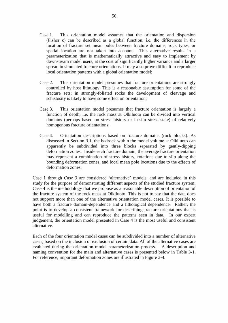
50

Case 1. This orientation model assumes that the orientation and dispersion

(Fisher κ) can be described as a global function; i.e. the differences in the

location of fracture set mean poles between fracture domains, rock types, or

spatial location are not taken into account. This alternative results in a

parameterization that is mathematically attractive and easy to implement by

downstream model users, at the cost of significantly higher variance and a larger

spread in simulated fracture orientations. It may also prove difficult to reproduce

local orientation patterns with a global orientation model;

Case 2. This orientation model presumes that fracture orientations are strongly

controlled by host lithology. This is a reasonable assumption for some of the

fracture sets; in strongly-foliated rocks the development of cleavage and

schistosity is likely to have some effect on orientation;

Case 3. This orientation model presumes that fracture orientation is largely a

function of depth; i.e. the rock mass at Olkiluoto can be divided into vertical

domains (perhaps based on stress history or in-situ stress state) of relatively

homogenous fracture orientations;

Case 4. Orientation descriptions based on fracture domains (rock blocks). As

discussed in Section 3.1, the bedrock within the model volume at Olkiluoto can

apparently be subdivided into three blocks separated by gently-dipping

deformation zones. Inside each fracture domain, the average fracture orientation

may represent a combination of stress history, rotations due to slip along the

bounding deformation zones, and local mean pole locations due to the effects of

deformation zones.

Case 1 through Case 3 are considered „alternative‟ models, and are included in this

study for the purpose of demonstrating different aspects of the studied fracture system;

Case 4 is the methodology that we propose as a reasonable description of orientation of

the fracture system of the rock mass at Olkiluoto. This is not to say that the data does

not support more than one of the alternative orientation model cases. It is possible to

have both a fracture domain-dependence and a lithological dependence. Rather, the

point is to develop a consistent framework for describing fracture orientations that is

useful for modelling and can reproduce the patterns seen in data. In our expert

judgement, the orientation model presented in Case 4 is the most useful and consistent

alternative.

Each of the four orientation model cases can be subdivided into a number of alternative

cases, based on the inclusion or exclusion of certain data. All of the alternative cases are

evaluated during the orientation model parameterization process. A description and

naming convention for the main and alternative cases is presented below in Table 3-1.

For reference, important deformation zones are illustrated in Figure 3-4.

51

Table 3-1. Listing of main and alternative cases evaluated during orientation model

parameterization. Alternative Case 4 was chosen as the recommended orientation

model alternative.

Case Lithology Deformation

zone (DZ) True depth Objective Code in figures

1A All Excluded All Global view 1A_All_NoZ

1B All Included All Global view 1B_All_WiZ

1C All Only DZ All Global view 1C_All_OnlyZones

2A Homogene

ous Excluded All Lithology 2A_Homogenized_Rock

2B Migmatite Excluded All Lithology 2B_Migmatite_Rock

2C Homogene

ous Excluded Below 150m Lithology 2C_Homogenized_Below150

2D Migmatite Excluded Below 150m Lithology 2D_Migmatite_Below150

3A All Excluded Above 150m Depth

dependence 3A_Above150

3B All Excluded Below 150m Depth

dependence 3B_Below150

3C All Excluded Every 150m Depth

dependence 3C_Between…

4

All Excluded Above or Below Zone BFZ098

Rock block model

4_...

4A All Excluded Above BFZ098 Rock block

model Upper block

4A_Above_Z098.

4B All Excluded Below BFZ098 Rock block

model 4B_Below_Z098

4C All Excluded All Rock block

model North-West

4C_BH_3_5_6_19_20_20B_21

4D All Excluded Above

BFZ055

Rock block model

South-East 4D_BH_8_9_23_23B_27_A5_Z055

4E All Excluded Below BFZ098 Rock block

model Secondary

4E_BH_8_17_24_38_B4_Z098

4F1 All Excluded Intermediate Rock volume

Rock block model

Intermediate

4F1_From_Z098_down_100m_B40

4F2 All Excluded Below

intermediate rock volume

Rock block model

Lower Block 4F2_Below_Z098+100m_B40

Bore hole All Excluded All Presentation of bore hole

data Bore_hole_KR…

Trench All Excluded All Presentation of trench data

Trench_KR…

52

3.2.2 Case 1: All fractures in all boreholes

The goal of Case 1 is to develop a statistical description of all fractures recorded in the

cored borehole array, regardless of rock type, depth, or fracture domain. The resulting

orientation model will represent a global ‘average’ model of bedrock fractures within

the Olkiluoto model volume, at the expense of local accuracy. Correspondingly, the

variance will be higher than for other alternative cases. There are three different sub-

alternatives inside Case 1. Case 1A (Figure 3-5) excludes fractures mapped as inside

modelled deformation zones, while Case 1B (Figure 3-6) includes these structures.

Finally, Case 1C (Figure 3-7) examines only the orientations of fractures inside

deformation zones. As the definition of a fracture domain explicitly excludes fractures

inside deformation zones, Cases 1B and 1C were included as descriptions for hypothesis

testing; they are not seriously evaluated as possible candidate orientation models.

In Case 1A, fracture orientations are dominated by a N-S elongated oval cluster, with a

mean pole orientation of (321°, 64°); we have termed this a ‘sub-horizontal’ cluster,

though in truth of fact it is actually described as ‘gently dipping’ (after Fleuty, 1964).

This pole cluster is classified as a ‘median cluster’ (Section 2.3.5). There are also two

steeply-dipping pole clusters, representing structures that strike roughly north-south

(267°, 9°) and east-west (354°, 7°). Both can be classified as median clusters. It is

important to note the extremely large variability in fracture orientations; this suggests

that fracture orientation is somewhat dependent on one or more spatially-varying

parameters. The remaining (Cases 2 – 4) model alternative cases are designed to

evaluate some of these potential controls on fracture orientation.

Figure 3-5. Terzaghi-compensated Fisher (1953) contours of fracture poles for

orientation model Case 1A.

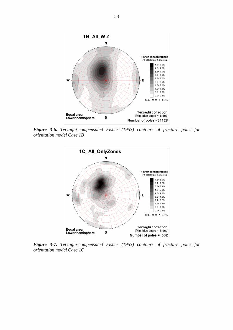
53

Figure 3-6. Terzaghi-compensated Fisher (1953) contours of fracture poles for

orientation model Case 1B

Figure 3-7. Terzaghi-compensated Fisher (1953) contours of fracture poles for

orientation model Case 1C

54

Figure 3-8. Stereoplots of the three different types (from left to right: regular, regular

folded, and irregular) of foliation found in cored borehole array at Olkiluoto. Figure is

taken from a Posiva working report (Milnes et al. 2006) describing a preliminary

evaluation of the geologic context of foliation at Olkiluoto.

However, it is possible that, at least in aggregate, the combination of the east-west

striking and subhorizontal pole clusters seen in Figure 3-5 and Figure 3-6 in fact

represent a girdle distribution of poles, suggesting large-scale folding or a dependence

of fracture orientation on a geologic texture (such as foliation or schistosity). Geologic

investigations at Olkiluoto (Milnes et al., 2006) have suggested that a strong, pervasive

foliation exists in the gneissic and migmatitic units that on average strike roughly north-

northeast (Figure 3-8) with gentle to moderate east-southeast dips. However, the

hypothesis of structural dependence of fracture orientation has not been formally

evaluated or quantified during the initial DFN modelling efforts; it is anticipated as a

component of the next stage of DFN model development.

The results of Case 1B are very similar to that of Case 1A; the inclusion of fractures

inside deformation zones has very little effect on the overall fracture orientation trends.

Case 1C, however, shows some interesting trends not seen in the previous two data sets.

There is possibly a weak fourth pole cluster striking northwest-southeast (approximate

orientation of 50°, 10°). Though we have not analyzed fractures inside deformation

zones in detail as they are outside the scope of the DFN modelling, it is possible that the

northwest-striking poles and the east-west striking poles might represent shear features

(Riedel shears) inside the footprint of the deformation zone.

Method for classifying fractures into sets by hard- and soft-sector assignment

Based on the preliminary results observed in the Case 1 stereoplots, a hard-sector

approach to the initial assignment of fracture poles to sets is adopted, with soft-

sectoring used for local refinement. A hard-sector assignment is a simple geometric

problem; if the trend and plunge of a fracture pole falls within a certain range of angles

that define the fracture set, it is assigned to that set. If the trend of the fracture pole is

0.01° larger than the set boundary, the pole is assigned to a different set. Pole

orientation is the only discriminator for set assignment.

The initial hard sectors for orientation model alternative Case 1A are presented below in

Figure 3-9. The hard sectors are defined as non-symmetric curves projected onto a

55

lower hemisphere plot. The curve will separate the fractures into one sub-horizontal set

and two sub-vertical sets. The curve is defined by four points with the following values

of trend and plunge in degrees: Point 1: 320°, 30°; Point 2: 30°, 35°; Point 3: 130°, 40°;

and Point 4: 220°, 40°. Note that the orientation set identifier in these set assignments

refers to the relative location of the poles on the hemisphere: fractures with poles

trending north (350° - 10°) with shallow (1° - 20°) plunges represent fractures striking

east-west and dipping steeply (70° – 89°) to the south.

A subhorizontal (SH) set is given by fractures with a plunge inside of the curve;

A subvertical N-S set is defined by poles north of points 1 and 2, and by

fractures south of points 3 and 4; and

A subvertical E-W set is defined by fractures west of points 4 and 1, and by

fractures east of points 1 and 2.

Figure 3-9. Division of fracture poles into orientation sets using the hard-sector

algorithm. Fracture poles are from orientation alternative Case 1A.

Once the poles (and their associated fractures) are initially assigned to orientation sets

through hard-sectoring, a local refinement around dense pole clusters using soft-

sectoring is used to determine the statistical properties of each fracture set (orientation

of the set mean pole and the calculation of the Fisher concentration parameter κ). A

mean pole for each orientation set is calculated for each borehole in the cored borehole

database; the mean pole describes the average orientation (trend, plunge) of the

fractures belonging to the selected set. The areas with large amounts of fractures are

defined as follows: For the sub-horizontal set 40% of the area is studied for the sub-

vertical sets 50% of the area is studied. By use of this approach soft-sectors were

56

defined around areas on the hemisphere with large numbers of fractures. The mean

poles and the quantifications of the shapes of pole clusters are calculated by use of the

eigenvector method (See Fisher et al., 1987 or Davis, 2002). The orientation analysis

and set division is performed on Terzaghi-compensated data (see Section 2.3.3).

The number of fractures in each of the fracture orientation sets is calculated as a

percentage of all fractures after Terzaghi compensation outside of deformation zones

with a valid orientation measurement. Case 1A produces the following results for the

three sets: subhorizontal set = 65%; subvertical North-South set = 17%; and subvertical

East-West set = 17%.

Figure 3-10 illustrates the results of both the hard- and soft-sector analysis. The first

item to recognize is that even though fracture orientations appear to fall into simple

patterns on stereoplots, when viewed on a borehole-by-borehole basis, there is

significant variation in the orientation of the mean pole for a given fracture set. The red

points in Figure 3-10 represent the location of the mean pole for a single borehole,

while the cyan dots indicate the location of the mean pole for the fracture set for all data

records combined. The confidence cone around the clusters of borehole set mean poles

is quite large; it generally has a radius of 15° – 20°. For at least five different boreholes,

the solid angle between the orientation of the mean pole of the SH set is greater than 20°

from the average orientation of the SH set for all data combined; in addition, the dip

direction for these five boreholes changes from north to south.

Figure 3-10. Fracture poles from orientation alternative Case 1A, with mean pole

orientations calculated for sets in individual boreholes (red) and for each set using all

available data (cyan).

57

The high degree of variability in the locations of the individual borehole set mean poles

suggests that a global orientation model for all boreholes, lithologies, and fracture

domains would be a poor choice for DFN modelling; it would be very difficult to match

local fracture orientation patterns.

3.2.3 Case 2: fracture orientation correlated to bedrock lithology

The analyses conducted during the assessment of Case 2 are designed to test fracture

orientation dependence on bedrock lithology. The bedrock described in the Olkiluoto

geological site model (Posiva, 2008) consists of high-grade metamorphic supracrustal

rocks derived from epiclastic (sedimentary) and pyroclastic (volcanic) sources. The

majority of the bedrock at Olkiluoto (Figure 1-1) can be roughly divided into five

different classes:

Migmatitic gneiss;

Tonalitic-granodioritic-granitic (TGC) gneiss;

“Other” gneiss (mica gneiss, quartz gneiss, mafic gneiss);

Pegmatitic granites; and

Diabase dykes

In the database of fractures and rock data from cored boreholes, fracture host lithology

is indicated by a series of rock codes (Table 3-2). For the version 1.0 geological DFN

model, bedrock lithology was divided into two classes, Migmatite and Homogeneous,

based on the assumption that the gneisses are more strongly foliated as a group than the

migmatites; the degree of partial melting reached within the migmatites may have been

enough to eliminate some of the foliation or schistosity. Diabase dykes were excluded

from the analysis due to a lack of fracture data. Future geological DFN models will look

at the differences between lithological units (TGC versus other gneisses) in greater

detail.

Table 3-2. Posiva lithology codes and rock-type classes used in the geological DFN

analysis.

Posiva Code Rock Type

VGN Migmatite

DGN Migmatite

MGN Homogenized

TGG Homogenized

QGN Homogenized

MFGN Homogenized

PGR Homogenized

SGN Migmatite

MDB Not Considered

KFP Not Considered

CRUSH Not Considered

58

Alternative Case 2 is divided up into several sub-cases, based on the following criteria:

Case 2A represents all fractures occurring in Homogenized rock;

Case 2B represents all fractures occurring in Migmatite rock.

Case 2C represents all fractures occurring in Homogenized rock and below a

true depth of 150 m (from ground surface); and

Case 2C represents all fractures occurring in Migmatite rock and below a true

depth of 150 m (from ground surface).

When considering all depths (Cases 2A and 2B) a comparison of Figure 3-11 and

Figure 3-12 and the hard-sector division results (Table 3-3) suggests that there are some

differences in the pattern of fracture poles, but that these differences are quite subtle.

The subhorizontal pole set in the Homogenized rock class has both a more elongated

shape and a lesser relative intensity, when compared to the Migmatite class. The

orientations of the other fracture set mean poles are very similar for both rock types.

When considering only the rock masses below a true vertical depth (TVD) of 150 m, the

results are rather similar to the results produced for all depths. An interesting difference

is that the pole concentration for the subhorizontal set is bimodal, suggesting either the

overprinting of a younger subhorizontal set atop an existing subhorizontal set, rotation

of crustal blocks, or perhaps bolstering the concept of fracture-domain specific set

orientations (i.e. we are looking at a pattern formed by two different rock blocks merged

together onto the same plot).

Figure 3-11. Case 2A: All fractures inside “Homogenized” rock class. Left plot

illustrates Fisher contours of fracture poles, while the right plot illustrates the results of

the hard-sector set assignment.

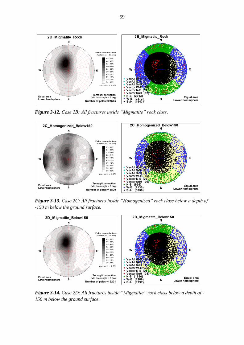
59

Figure 3-12. Case 2B: All fractures inside “Migmatite” rock class.

Figure 3-13. Case 2C: All fractures inside “Homogenized” rock class below a depth of

-150 m below the ground surface.

Figure 3-14. Case 2D: All fractures inside “Migmatite” rock class below a depth of -

150 m below the ground surface.

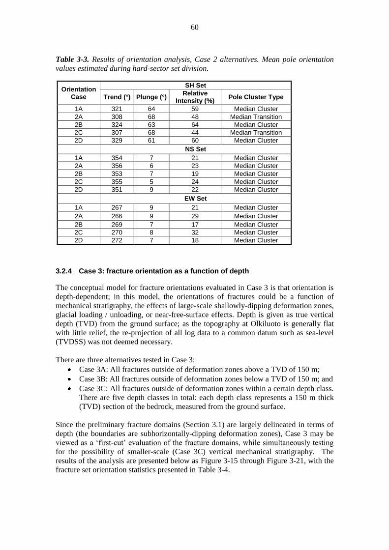
60

Table 3-3. Results of orientation analysis, Case 2 alternatives. Mean pole orientation

values estimated during hard-sector set division.

Orientation Case

SH Set

Trend (°) Plunge (°) Relative

Intensity (%) Pole Cluster Type

1A 321 64 59 Median Cluster

2A 308 68 48 Median Transition

2B 324 63 64 Median Cluster

2C 307 68 44 Median Transition

2D 329 61 60 Median Cluster

NS Set

1A 354 7 21 Median Cluster

2A 356 6 23 Median Cluster

2B 353 7 19 Median Cluster

2C 355 5 24 Median Cluster

2D 351 9 22 Median Cluster

EW Set

1A 267 9 21 Median Cluster

2A 266 9 29 Median Cluster

2B 269 7 17 Median Cluster

2C 270 8 32 Median Cluster

2D 272 7 18 Median Cluster

3.2.4 Case 3: fracture orientation as a function of depth

The conceptual model for fracture orientations evaluated in Case 3 is that orientation is

depth-dependent; in this model, the orientations of fractures could be a function of

mechanical stratigraphy, the effects of large-scale shallowly-dipping deformation zones,

glacial loading / unloading, or near-free-surface effects. Depth is given as true vertical

depth (TVD) from the ground surface; as the topography at Olkiluoto is generally flat

with little relief, the re-projection of all log data to a common datum such as sea-level

(TVDSS) was not deemed necessary.

There are three alternatives tested in Case 3:

Case 3A: All fractures outside of deformation zones above a TVD of 150 m;

Case 3B: All fractures outside of deformation zones below a TVD of 150 m; and

Case 3C: All fractures outside of deformation zones within a certain depth class.

There are five depth classes in total: each depth class represents a 150 m thick

(TVD) section of the bedrock, measured from the ground surface.

Since the preliminary fracture domains (Section 3.1) are largely delineated in terms of

depth (the boundaries are subhorizontally-dipping deformation zones), Case 3 may be

viewed as a ‘first-cut’ evaluation of the fracture domains, while simultaneously testing

for the possibility of smaller-scale (Case 3C) vertical mechanical stratigraphy. The

results of the analysis are presented below as Figure 3-15 through Figure 3-21, with the

fracture set orientation statistics presented in Table 3-4.

61

The depth-dependence analysis shows little difference in terms of the orientations of the

subvertical sets as a function of depth, other than a very slight tendency of the EW set to

have shallower dips below 450 m TVD. The dominant orientation change is in the

subhorizontal set; however, the differences between depth classes are not very large. In

addition, even with oriented core and detailed image / BHTV logs, it can be quite

difficult to determine the correct strike orientation of subhorizontally-dipping fractures

in core. Munier and Stigsson (2007) indicated that the combination of:

variability of the diameter of the borehole;

uncertainty in the core mapping process;

uncertainty in the orientation of the borehole in space; and

uncertainty in the orientation of the image logs in space;

could combine, in some cases, to produce a strike uncertainty of up to 180° (though

actual orientation uncertainty was generally reported as much smaller) for all fractures.

The uncertainty is likely (but not tested or quantified at Olkiluoto) biased strongly

towards fractures intersecting the core at nearly a right angle, as that produces the

smallest intersection area within the core and the thinnest feature within the image logs.

The trend of the mean pole for the SH set in the series of orientation Case 3 alternatives

varies by up to +/- 10° between depth classes, with little variability in the mean pole

plunge with depth until a TVD of 600 m. Below 600 m, the plunge of the SH set

shallows by 5° – 10°; this implies that the dip of the fractures in the SH set is increasing

with increasing depth. When considering the shape of the sub-horizontal concentration

of poles there are obvious differences; noteworthy is that between depths 450 m and

600 m the pole clusters representing SH set demonstrates an elongated shape with two

local maxima. It was also observed that the relative intensity of fractures in the SH set

in the cored boreholes is largest (64%) near the ground surface (above a depth of 150m).

At sub-repository horizon depths (>750 m), the relative intensity of fractures in the SH

set seems to decrease significantly (33%).

Figure 3-15. Fracture contoured polar stereoplot (left) and hard-sector set division

results (right) for orientation alternative case 3A.

62

Figure 3-16. Fracture contoured polar stereoplot (left) and hard-sector set division

results (right) for orientation alternative case 3B.

Figure 3-17. Fracture contoured polar stereoplot (left) and hard-sector set division

results (right) for orientation alternative case 3C1, representing a depth interval from

150 m to 300 m.

Figure 3-18. Fracture contoured polar stereoplot (left) and hard-sector set division

results (right) for orientation alternative case 3C2, representing a depth interval from

300 m to 450 m.

63

Figure 3-19. Fracture contoured polar stereoplot (left) and hard-sector set division

results (right) for orientation alternative case 3C3, representing a depth interval from

450 m to 600 m.

Figure 3-20. Fracture contoured polar stereoplot (left) and hard-sector set division

results (right) for orientation alternative case 3C4, representing a depth interval from

600 m to 750 m.

Figure 3-21. Fracture contoured polar stereoplot (left) and hard-sector set division

results (right) for orientation alternative case 3C5, representing a depth interval from

750 m to 1000 m. Note that due to the sparse data coverage in this portion of the

Olkiluoto model volume, the depth class has increased in size to 250 m TVD.

64

Table 3-4. Results of orientation analysis, Case 3 alternatives. Mean pole orientation

values estimated during hard-sector set division.

Orientation Case

Trend (°) Plunge (°) Relative

Intensity (%) Pole Cluster Type

SH Set

1A 321 64 59 Median Cluster

3A 318 64 64 Median Cluster

3B 325 63 54 Median Transit

3C1 321 63 55 Median Cluster

3C2 328 65 54 Median Transit

3C3 317 64 57 Median Transit

3C4 337 57 58 Median Cluster

3C5 340 52 33 Median Transit

NS Set

1A 354 7 21 Median Cluster

3A 359 8 18 Median Cluster

3B 353 7 22 Median Cluster

3C1 353 7 21 Median Cluster

3C2 351 8 24 Median Cluster

3C2 176 2 22 Median Cluster

3C4 6 7 28 Median Cluster

3C5 344 2 21 Median Transit

EW Set

1A 267 9 21 Median Cluster

3A 263 8 18 Median Cluster

3B 270 8 23 Median Cluster

3C1 273 8 23 Median Cluster

3C2 270 7 22 Median Cluster

3C3 264 9 22 Median Cluster

3C4 266 12 14 Median Transit

3C5 85 5 45 Median Cluster

(1) Amount of fractures in a fracture set, in relation to all fractures in all sets. Calculated by use of Terzaghi correction.

(2) Only approx 618 mapped fractures in this depth class; therefore the results are more uncertain than for the other depth classes

3.2.5 Case 4: fracture orientation as a function of fracture domain

As previously discussed during the introduction of the proposed fracture domains at

Olkiluoto (Section 3.1), an orientation description based on rock blocks is conceptually

a very attractive approach. Fracture domains fundamentally bind the rock mass into sub-

volumes of relatively homogeneous fracturing (at least in terms of fracture orientation

and relative set intensity), which can reduce overall model variability. Furthermore, it is

highly likely that, as at the two proposed Swedish hard-rock sites of Forsmark and

Laxemar, most of the rock fractures are thought to be quite old (Fox et al., 2007; La

Pointe et al., 2005) and largely represent stresses present during the tectonic evolution

of the site. Deformation zones have the potential to affect the localized stress state in the

bedrock enough to influence the orientation of fractures, to create additional subsets not

found elsewhere (i.e. additional structures found in the hanging wall and footwall of

65

faults related to deformation along the fault), and can also provide for bulk-scale (block)

crustal rotations, which can produce fracture orientation patterns ‘rotated’ or out-of-

phase with adjacent blocks.

A preliminary analysis of fracture orientation and relative intensity patterns subdivides

the bedrock at Olkiluoto into three fracture domains (Figure 3-2), separated by large

subhorizontally-dipping deformation zones:

1. Upper rock block: This fracture domain extends from the ground surface down

to deformation zone BFZ098; a ‘respect distance’ of 50 m parallel to this zone

has been applied, within which fractures are either excluded from analysis, or

included in the ‘intermediate’ fracture domain;

2. Intermediate rock block: This fracture domain describes a volume of rock

roughly bounded by deformation zones BFZ098 and BFZ080; and

3. Lower rock block: This fracture domain represents the volume of rock in the

footwall of the BFZ080-BFZ098 fault system, down to a depth of 1,000 m

below the ground surface.

Note that the development of the Case 4 orientation model alternatives occurred

simultaneously with the development of the fracture domain model; both the locations

of set mean poles and the relative intensity of sets was key to defining the fracture

domains. There are seven different orientation model sub-cases within the Case 4

orientation alternatives evaluation; the sub-cases vary in terms of the number of

boreholes used in the parameterization, the depth cut-offs applied, and which fracture

domain / rock block was included. The sub-cases consist of:

Case 4A: Includes all boreholes that penetrate deformation zone BFZ098, but

only includes fractures above this structure (i.e. in the Upper fracture domain);

Case 4B: Includes all boreholes that penetrate deformation zone BFZ098, but

only includes fractures below this structure (i.e. in the Lower fracture domain);

Case 4C: This case evaluates the hypothesis that fractures to the west-northwest

of the mapped limits of BFZ098 should be extremely similar to those mapped in

the footwall of BFZ098. This case includes data from cored boreholes OL-KR3,

OL-KR5, OL-KR6, OL-KR19, OL-KR20/20B, and OL-KR21;

Case 4D: This case considers block translations / rotations caused by

deformation zone BFZ055; the hypothesis is that fractures on the west-northwest

side (footwall) of BFZ055 will be very similar to Case 4A (affected by

BFZ098), but that fractures on the east-southeast side of BFZ055 will show

changes in the orientations of the fracture set mean poles due to block rotation.

Case 4D utilizes boreholes OL-KR8, OL-KR9, OL-KR23/23B, and OL-KR27;

Case 4E: This case examines the existence of a secondary subhorizontal pole

cluster observed in deeper cored boreholes; the presence of an ovoid and

66

elongated clustering of fracture poles below BFZ098 was noted in Case 4B.

Utilizing boreholes OL-KR8, OL-KR17, OL-KR24, and OL-KR38, an analysis

is attempted to determine if there is a secondary ‘set’ hidden in the data, or if the

shape of the pole cluster truly represents the data variability.

Case 4F1 / Case 4F2: These two cases evaluate the hypothesis that the zone of

influence for BFZ098 extends a good distance (~100 m) vertically away from

the fault plane. Case 4F1 looks at the rock volume above this zone to the ground

surface (and so includes the influence zone of BFZ080), while Case 4F2

includes the rock below this 100 m offset zone.

Figure 3-22. Cored boreholes that penetrate through BFZ098 (the blue zone). All are

included in either Case 4A or Case 4B. The interpreted orientation (pole trend, plunge)

of deformation zone BFZ098 is (320°, 65°).

Figure 3-23. Case 4A: All fractures in the Upper fracture domain (above BFZ098). The

yellow circle denotes the approx orientation of BFZ098.

67

Figure 3-24. Case 4B: All fractures in the Lower fracture domain (below BFZ098). The

yellow circle denotes the approx orientation of BFZ098.

A comparison of Figure 3-23 and Figure 3-24 show that the orientations of

subhorizontally-dipping fractures are strikingly different above and below deformation

zone BFZ098. The average plunge of the mean pole is roughly the same, but there is

almost a 30° rotation in the pole trend (representing a change in strike of the

subhorizontally-dipping fractures) below BFZ098. In addition, the variability of the

location of the mean pole is much higher beneath BFZ098; note the increased spread in

the distribution of set mean pole by borehole (Figure 3-24). Finally, the existence of a

north-dipping, east-west striking secondary subhorizontal fracture set in the Lower

fracture domain is suggested by the appearance of a second pole cluster (Figure 3-24).

Given that the solid angle between the mean poles of the two subhorizontal clusters is

greater than 60°, we find it unlikely that the secondary cluster is an artefact or just a

symptom of higher than expected orientation variability. The shape of the

concentrations of poles above BFZ098 is a classified as a median cluster, but below

BFZ098 the pole concentration is elongated and classified as a median transition, this

pole-concentration will be analysed in Case 4E and the following Case 4F.

Figure 3-25. Case 4C: Boreholes OL-KR3, OL-KR5, OL-KR6, OL-KR19, OL-KR20 and

OL-KR21. Deformation zones BFZ098 and BFZ080 are coloured purple and teal,

respectively.

68

Figure 3-26. Case 4C: Orientations of fractures west-northwest of the mapped extent of

deformation zone BFZ098.

If the hypothesis that the combination of deformation zones BFZ098 and BFZ080 work

to produce an Upper and Lower fracture domain at Olkiluoto, then it stands to reason

that the fracture orientations in the rock volume west-northwest of the mapped extents

of these structures (Figure 3-25) should be most similar to fracture orientations

observed in the Lower fracture domain (i.e. this domain reaches to the ground surface).

This hypothesis was evaluated in Case 4C. The results (Figure 3-26) suggest that the

shapes of the subhorizontal pole cluster below BFZ098 (Case 4B) and west of BFZ098

(Case 4C) are similar; however, there appears to be less variability in the orientation of

the mean pole in Case 4C than in Case 4B, and the fracture poles in Case 4C form a

median cluster, not an elongated cluster as in Case 4B. The observed fracture

orientation patterns support the fracture domains as defined. There appears to be a very

slight (~10°) potential rotation in the location of the mean poles of the two subvertical

fracture sets between Case 4B and 4C; however, this difference is likely well within the

probable measurement uncertainty and the degree of spatial variability inherent in any

geologic system.

Figure 3-27. Case 4D: Boreholes OL-KR8, OL-KR9, OL-KR23, OL-KR23B and OL-

KR27. Deformation zone BFZ098 is coloured purple while deformation zone BFZ055 is

coloured dark red.

69

Figure 3-28. Case 4D: Orientations of fractures east-southeast of deformation zone

BFZ055.

Case 4D was designed to evaluate two questions: do fracture orientations change east of

deformation zone BFZ055 (the dark red subvertical zone depicted in Figure 3-27), and,

if they do not, can the orientation pattern be explained in the context of the hypothesized

fracture domains. If BFZ055 does not act as a fracture domain boundary, then the

fractures in boreholes OL-KR8, OL-KR9, OL-KR23, OL-KR23B and OL-KR27 should

show a general orientation pattern characteristic of the Upper fracture domain (Case

4A).

Figure 3-28 illustrates that the fracture pole orientations and relative set intensities for

the subhorizontal set are in fact quite similar to those inside the hypothesized Upper

fracture domain (Figure 3-23), and do not appear dramatically different on one side of

BFZ055 or the other. This provides additional qualitative support for the suggested

fracture domains. It is more difficult to come to conclusions on the orientations of the

poles making up the two subvertical fracture sets in Case 4D, given the large amount of

dispersion in the data. However, the estimated mean pole orientations are within +/- 5°

of those calculated in Case 4A (Table 3-5).

A remaining issue to be addressed in the Case 4 orientation alternatives is the observed

elongated shape of the subhorizontally-dipping pole clusters in the Intermediate and

Lower fracture domains (i.e. beneath deformation zone BFZ098). There are two obvious

possibilities to explain the shape created by the subhorizontally-dipping fracture poles:

either the poles are not Fisher-distributed (i.e. they follow a girdle distribution such as

Bingham or Bivariate Normal that represent fold structures), or that there is more than

one subhorizontal set that is ‘smearing out’ the data. For the version 1.0 geological DFN

model, it was decided to use only univariate Fisher distributions to parameterize fracture

orientations (Section 2.1.2); as such, the use of alternative hemispherical probability

distributions was not evaluated.

To test the possibility that the subhorizontal fracture set can be subdivided into two or

more sets (based largely on pole trend / fracture strike), orientation alternative cases 4E,

4F, and 4F2 were evaluated. In evaluating all fractures beneath deformation zone

BFZ098 (Case 4B), there appears to be two pole clusters that dominate the

70

subhorizontal set: a dominant north-plunging (representing fractures dipping to the

south) cluster and a subordinate south-plunging (representing fractures dipping to the

north) cluster. The subordinate cluster has been evaluated using a theoretical circle

(Figure 3-29) projected on the hemisphere, with a central axis orientation of (210°, 70°)

and a radius of 15°. Approximately 903 fracture poles fall within this circle; most of the

poles come from boreholes OL-KR1, OL-KR8 and OL-KR29.

However, if we consider fracture intensity (P10) instead of fracture count, we

compensate for the fact that the three boreholes with the highest fracture count also have

the longest lengths beneath BFZ098. Boreholes OL-KR8, OL-KR17, OL-KR24, and

OL-KR38 show the highest P10 intensity inside the theoretical circle representing the

potential subordinate cluster; these four boreholes are used to define sub-case 4E

(Figure 3-30). The results of Case 4E are presented below in Figure 3-31 and Table 3-

5, but in principal, we recognize that these four boreholes, along with OL-KR1 and OL-

KR29, illustrate the basic orientation patterns seen in the Intermediate fracture domain.

The principle exception in Case 4E is the North-South set; average pole plunge in this

set is 10° - 20° greater than in the other alternative model cases. It is probably that this

is largely an artefact of the hard-sectoring process, and that many of the observed

fractures attributed to the North-South set in this case are in fact members of a diffuse

Subhorizontal set; this will be tested in a future revision of the geological DFN.

Figure 3-29. Evaluation of multiple subsets within the subhorizontal set of fracture

poles using a theoretical circle projected on the hemisphere. This plot considers only

fractures recorded in cored borehole sections beneath deformation zone BFZ098.

71

Figure 3-30. Case 4E: Boreholes OL-KR8, OL-KR17, and OL-KR24 (OL-KR38 not

shown).

Figure 3-31. Case 4E: Fracture poles in boreholes OL-KR8, OL-KR17, OL-KR24, and

OL-KR38 at elevations beneath deformation zone BFZ098.

The boreholes studied in Case 4E do not extend very deep below deformation zone

BFZ098. As such, it is possible that the observed secondary subhorizontal pole clusters

which dominate the dataset are in fact due to the existence of a large damage zone

around BFZ098. This hypothesis is strengthened by the observation that the secondary

cluster does not occur in orientation model alternative Case 4C (Figure 3-26); the

secondary cluster should not appear in Case 4C if they represent fractures occurring

only in a damage zone beneath BFZ098, as the boreholes studied in Case 4C do not

penetrate BFZ098. Cases 4F1 and 4F2 were established to evaluate this hypothesis.

Case 4F1 considers all boreholes that penetrate through deformation zone BFZ098,

within a hypothetical rock volume (Figure 3-32) extending 100 m perpendicular beneath

the modelled lower surface of BFZ098; this case includes the rock mass between zones

72

BFZ080 and BFZ098 (the Intermediate fracture domain). Case 4F2 utilized all

boreholes penetrating through deformation zone BFZ098, but used only data taken from

the Lower fracture domain (i.e. at depths greater than the 100 m surface used in Case

4F1, c.f. Figure 3-2).

Figure 3-32. Cases 4F1 and 4F2. The pink surface represents the bottom of a 100m

zone (the Intermediate fracture domain) extending downwards from BFZ098 (purple).

Deformation zone BFZ080 is the light green structure.

Figure 3-33. Case 4F1: Fracture poles from borehole sections within the Intermediate

fracture domain.

73

Figure 3-34. Case 4F2: Fracture poles from borehole sections within the Lower

fracture domain (i.e. beneath the 100 m thick zone defined in the footwall of BFZ098).

Contour and polar stereoplots in Figure 3-33 and Figure 3-34 illustrate the results of

Case 4F1 and Case 4F2, respectively, while the orientations (trend, plunge) of the

cluster mean poles are presented in Taable 3-5. These two cases show that both the

location of the mean pole of the subhorizontal sets and the relative intensity (if one

assumes that there are in fact two different subhorizontal sets) are different in the

Intermediate and Lower fracture domains; the Intermediate fracture domain shows a

bias towards north-dipping, east-southeast-striking fractures, while the Lower fracture

domain shows a bias towards south-dipping, roughly east-west striking fractures. The

orientation patterns seen in Case 4F2 are quite similar to those seen in Case 4B (Figure

3-24); this gives support to the concept of the Intermediate fracture domain as an

enlarged damage zone in the footwall of BFZ098. What is interested is that the average

orientations of the subhorizontal fractures in the Intermediate fracture domain (Case

4F1) are not the same as the average orientation of BFZ098 (320°, 85°); they feature

similar dips, but are 30° - 70° rotated counter-clockwise relative to the fault surface. As

of this version of the Olkiluoto DFN model, a process to explain this rotation has not yet

been identified.

Little to no significant difference is seen in the two subvertical fracture sets, except that

in the Intermediate fracture domain, there *may* be a bimodal distribution of east-west

trending poles; the aggregated poles of all fractures in the Intermediate fracture dome

show two weak clusters separated by an approximately 30° solid angle. This suggests

that, at least in the Intermediate fracture domain, the East-West set could represent

Riedel R-shears formed in response to north-south compression. Further evaluation and

correlation with other shear indicators in the borehole data (mineral lineation,

orientation of ductile shear zones) would need to be evaluated to confirm this

hypothesis. No obvious difference was noted in the North-South set of poles, save that

the relative intensity of the North-South set is less in the Lower fracture domain (Case

4F2) than in the Intermediate fracture domain (Case 4F1).

74

Table 3-5. Fracture orientation analysis results for Cases 4A, 4B, 4C, 4D and 4F. Case

1A is included for reference.

Orientation Case

Trend (°) Plunge (°) Relative

Intensity1 (%)

Pole Cluster Type

SH Set

1A 321 64 59 Median Cluster

4A 313 62 62 Median Cluster

4B 321 65 53 Median Transit

4C 332 64 62 Median Transit

4D 308 62 57 Median Cluster

4E 204 70 62 Median Cluster

4F1 273 72 53 Median Transit

4F2 328 60 53 Median Transit

NS Set

1A 354 7 21 Median Cluster

4A 351 3 18 Median Cluster

4B 359 5 24 Median Cluster

4C 356 8 19 Median Cluster

4D 351 1 21 Median Cluster

4E 191 22 21 Median Cluster

4F1 181 2 27 Median Cluster

4F2 358 7 23 Median Cluster

EW Set

1A 267 9 21 Median Cluster

4A 276 12 20 Median Cluster

4B 266 5 23 Median Cluster

4C 80 0 18 Median Cluster

4D 274 15 21 Median Cluster

4E 261 8 17 Median Cluster

4F1 81 0 20 Median Cluster

4F2 269 7 24 Median Cluster

(1) Amount of fractures in a fracture set, in relation to all fractures in all sets. Calculated by use of Terzaghi correction.

3.2.6 Fracture orientation model

The variability of fracture orientations are encompassed through the use of

hemispherical probability distributions, which describe the orientation (trend, plunge) of

the mean pole, as well as a description of the dispersion (measure of clustering) around

this pole. As indicated in the Model Assumptions (Section 2.1.2), univariate Fisher

probability distributions are used for all fracture sets in the version 1.0 Olkiluoto

geological DFN model. The pole concentrations used to delineate fracture sets presented

in the previous section are not perfectly circular; in particular, the subhorizontal fracture

set is poorly parameterized using a univariate Fisher distribution. However, for reasons

previously discussed in the DFN model Assumptions section, univariate Fisher

distributions have some very attractive qualities (simple, computationally efficient, easy

to understand and implement in software) that, at least in the version 1.0 Olkiluoto

geological DFN, outweigh the disadvantages.

75

The results of the orientation analysis support the division of the rock mass at Olkiluoto

into three distinct fracture domains. As such, the recommended orientation model

parameterization is based on the Case 4 model alternatives. The recommended

orientation models (Fisher distribution parameters are summarized in Table 3-6) are:

Upper fracture domain: For the rock volume above deformation zone BFZ098, case 4A

should be used. This is also valid for regions in the local model volume east and south

of the mapped extent of BFZ098.

Intermediate fracture domain: For the rock volume extending downwards from

deformation zone BFZ098 approximately 100 m perpendicular to the zone, Case 4F1

should be used.

Lower Fracture Domain: For the rock volume beneath the Intermediate fracture domain

to the bottom of the current model extents (~ -1100 m elevation), case 4F2 should be

used. This is also valid for regions in the local model volume north and west of the

mapped extent of BFZ098.

Table 3-6. Version 1.0 geological DFN orientation model parameters

Fracture Domain

SH Set NS Set EW Set

Trend (°)

Plunge (°)

κ Trend

(°) Plunge

(°) κ

Trend (°)

Plunge (°)

κ

Upper 313 62 7.8 350 5 8.1 277 5 8.1

Intermediate 273 72 6.2 181 2 5.9 81 0 5.5

Lower 328 60 7 358 7 7 269 7 6.6

3.2.7 Orientation model applied to trenches, outcrops, and the ONKALO tunnel

At the Olkiluoto site, sedimentary overburden has been removed (as of late 2007 / early

2008) along eleven trenches and two outcrops (OL-TK10 and OL-TK11). Properties of

fractures (termination style, host lithology, trace length, orientation, mineralization and

degree of alteration) exposed in the resulting bedrock outcrops were recorded.

Orientations were available in the provided raw databases for most, but not all, mapped

outcrop and trench fractures. Data from the outcrops and trenches are presented below

in Table 3-7, while the recorded facture orientations and set divisions are presented in

Figure 3-35 through Figure 3-37.

76

Table 3-7. Outcrops and trenches at Olkiluoto where detailed fracture mapping was

performed (as of early 2008).

Trench ID Number of Fractures

# of Fractures with orientation data

Section Length (m)

OL-TK1 367 367 403.3

OL-TK2 415 415 415.4

OL-TK3 618 615 681.5

OL-TK4 654 653 828.6

OL-TK5 115 115 No data

OL-TK6 134 134 No data

OL-TK7 202 201 271.2

OL-TK8 1731 1730 1221.5

OL-TK9 1197 1195 462.3

OL-TK10* 642 635 No data

OL-TK11* 6285 6129 6346.6

OL-TK12 238 238 202.4

OL-TK13 649 649 544.4

* Outcrops

Figure 3-35. Fisher-contoured stereonet (left) and hard-sectored pole plot (right) of all

fractures mapped on surface trenches at Olkiluoto. Note that OL-TK10 and OL-TK11

are considered outcrops (rectilinear shape) and so are not included in these plots.

77

Figure 3-36. Fisher-contoured stereonet (left) and hard-sectored pole plot (right) of

outcrop OL-TK10.

Figure 3-37. Fisher-contoured stereonet (left) and hard-sectored pole plot (right) of

outcrop OL-TK11.

Neither the outcrop fracture data nor the trench data are directly used in the orientation

analysis; rather, they are used as a check against the fracture domain and orientation

models derived from borehole data. The bedrock surface is assumed to be entirely

within the Upper fracture domain, which already has excellent borehole coverage. As

such, a decision was made, unless significant differences were noted during data

analysis, to impose the orientation models from boreholes upon the surface data.

Fractures were assigned to one of three sets (SH, NS, EW) using the hard sectoring

approach; the resulting aggregate stereonets and orientation statistics are presented

below as and Table 3-8.

78

Table 3-8. Fracture set parameters for aggregated trench and outcrop data at

Olkiluoto.

Orientation Case Trend

(°) Plunge

(°) Relative

Intensity1 (%)

Pole Cluster Type

SH Set

Case 4A (Upper Domain)

313 62 62 Median Cluster

All Trenches 327 62 48 Median Cluster

NS Set

Case 4A (Upper Domain)

351 3 18 Median Cluster

All Trenches 355 5 38 Median Cluster

EW Set

Case 4A (Upper Domain)

276 12 20 Median Cluster

All Trenches 270 6 28 Median Transit

(1) Amount of fractures in a fracture set, in relation to all fractures in all sets. Calculated by use of Terzaghi correction.

Figure 3-38. Fisher-contoured stereonet (left) and hard-sectored pole plot (right) of all

trench and outcrop data combined. This composite data set was used to derive the

orientation statistics presented in Table 3-8.

The average orientations as given in the above discussed figure and table are not

significantly different from the average orientation of the fractures in the boreholes

above zone BFZ098 (Case 4A). Qualitatively, the stereonet patterns look extremely

similar to those seen in borehole sections penetrating the Upper fracture domain; this

bolsters the current fracture domain conceptualization and supports the orientation

model as parameterized. The trends of the fracture set mean poles vary by 5° - 10°;

however the plunges are quite consistent. Outcrop OL-TK10 is the only significant

anomaly; the pole clusters suggest that fracturing at this outcrop is somewhat different

than in the trenches and at OL-TK11. In particular, the NS pole set (representing

fractures striking East-West) is largely absent, and, in its place appears a set of steeply-

79

dipping northeast-striking fractures. We hypothesize that the fracture pattern at OL-

TK10 is affected by deformation stage D3 shearing in the eastern half of the island; the

northeast strike of most of the structures follows a similar orientation to the F4 axial

surfaces postulated for this part of the island (Figure 4-14, Mattila et al., 2008). Data

from this outcrop will be re-examined in further detail in future geological DFN models.

The fracture set relative intensities calculated from outcrop and trench data are

significantly different from those calculated from the borehole data. In particular, the

NS subvertical set is more intense at the ground surface than at depth, at the expense of

the SH set. We suspect that the differences between the two data sets are largely due to

sampling bias. Outcrop surveys perpendicular to the ground surveys are highly biased

against sampling subhorizontally-oriented fractures, just as near-vertical boreholes are

biased against sampling subvertical fractures. The Terzaghi correction can be used to

compensate for orientation bias in a borehole, but is far less useful in dealing with

outcrop data. Nevertheless, the differences in relative fracture intensity between

borehole and outcrop will be formally addressed in a future geological DFN revision.

Orientation data from the ONKALO tunnel is not directly used in the orientation model

parameterization, largely because the tunnel only samples the (already) well-sampled

Upper fracture domain, as well as the fact that the orientations recorded along the tunnel

are viewed by the DFN team as significantly more uncertain due to issues with the

quality and repeatability of the available mapping data. As such, the ONKALO tunnel

orientations (Figure 3-39) were also used as a qualitative check against the orientation

and fracture domain model derived predominantly from boreholes. The results of the

tunnel mapping appear fairly similar to the description of the Upper fracture domain

(orientation alternative Case 4A); the principal fracture set (SH) appears to be largely

parallel to the foliation observed in this region of Olkiluoto (Figure 4-15, Mattila et al.,

2008) with some variability noted in the mean pole locations of the two subvertical

fracture sets. It is interesting to note that the overall dispersion of all sets is quite high in

the ONKALO tunnel data. There are also suggestions of systematic data artefacts in

fracture orientations; note the linear N-S feature in Figure 3-39, as well as the distinct

lack of structures of all plunge values between 180° and 185°. This discrepancy will be

investigated during the data compilation stages of future geological DFN models.

Figure 3-39. Fracture orientations recorded in the ONKALO tunnel.

80

3.3 Fracture intensity model

3.3.1 Model Implementation

The methodology for the analysis and parameterization of fracture intensity based on

borehole and outcrop data in the version 1.0 Olkiluoto geological DFN model is

described in detail in Section 2.5. As with the orientation model, the intensity model is

focused on describing the intensity (P10Te as a proxy for P32) in the three identified

fracture domains using available cored borehole data. The ONKALO tunnel and surface

outcrops are instead used to calibrate and validate the proposed. As with the orientation

model / fracture domain model, the analysis of fracture intensity is linked with fracture

size. The intensity model and size model calibration were done simultaneously, in an

iterative approach that is described in Chapter 4.

Fracture intensity is assumed to be a function of fracture set, fracture domain, and depth

below the ground surface. Host lithology, secondary mineralization, and degree of

bedrock alteration are assumed to have a second-order effect, though only lithologic

dependence has been tested in this version of the geological DFN. Future model

iterations will explore the connection between lithology, ductile deformation,

metamorphic history, and rock properties in more detail. The intensity analysis is based

principally on understanding the change in Terzaghi-compensated lineal fracture

intensity (P10Te) with depth and fracture domain.

Fracture intensity data from cored boreholes used in the intensity model

parameterization are described in Table 3-9. Note that fractures inside the core of

mapped deformation zones are excluded from the analysis. However, since no

systematic study or mapping of the so-called "transition" zone of increased fracturing

existed as of the completion of this study, there is a possibility that some 'deformation

zone fractures' have been included in the intensity analysis. This will be addressed in

future geological DFN model revisions. Only fractures with recorded orientations (dip,

dip direction translated to trend, plunge) are used in the intensity analysis; as intensity is

a fracture set property, fractures without recorded orientations cannot be assigned to a

set. Fractures with complete orientation data are termed "accepted" fractures in Table 3-

9. The key to the different columns and statistics in is presented below:

P10: Lineal fracture intensity, calculated as (N1 / LENGTH). This value is not

Terzaghi-compensated;

N1: Total number of recorded fractures in borehole;

N2: Number of accepted fractures;

N3: Total number of recorded fractures in borehole plus "daughter" fractures

added through Terzaghi compensation;

N4: Number of accepted fractures in borehole plus "daughter" fractures added

through Terzaghi compensation;

P10TE: Lineal fracture intensity, corrected for borehole orientation bias through

Terzaghi compensation, calculated as (N4 / LENGTH);

81

LENGTH: Length (measured depth, in meters) of the borehole from which

fractures have been used in the orientation analysis. This excludes sections of

the borehole inside mapped deformation zones.'

Table 3-9. Fracture counts and intensity in cored borehole array at Olkiluoto. Note that

this data is analogous to Case 1A from the orientation model analysis (all boreholes, all

domains).

Borehole N1 N2 N3 N4 P10 P10Te LENGTH

KR1 2039 1751 3095 2807 2 2.8 1000.7

KR2 2650 1971 3959 3280 2.5 3.1 1051.9

KR3 1363 942 1965 1544 2.7 3.1 502

KR4 1486 0 1486 0 1.6 0.0 901.4

KR5 1273 1068 1843 1638 2.3 3.0 554

KR6 1512 1264 2140 1892 2.5 3.2 600.6

KR7 1549 867 1967 1285 1.9 1.6 810.6

KR8 1420 1156 2122 1858 2.4 3.1 600.5

KR9 1254 1082 1821 1649 2.1 2.8 599.2

KR10 815 625 1207 1017 1.3 1.7 612.7

KR11 1399 986 2122 1709 1.4 1.7 1001.9

KR12 2615 2152 4580 4117 3.3 5.2 795.3

KR13 1864 1699 2903 2738 3.7 5.5 500

KR14 774 625 1084 935 1.5 1.8 513.3

KR15 569 496 873 800 1.1 1.5 517.7

KR16 339 282 527 470 2 2.8 169.7

KR17 248 221 339 312 1.6 2.0 156.6

KR18 140 112 220 192 1.1 1.5 125.3

KR19 1651 1515 2493 2357 3.1 4.4 536.2

KR20 986 952 1325 1291 2 2.6 494.4

KR21 1124 956 1714 1546 3.7 5.1 301

KR22 1713 1513 2172 1972 3.4 4.0 499.1

KR23 554 504 734 684 1.9 2.3 295.2

KR24 890 611 1079 800 1.6 1.5 549.6

KR25 1358 1247 1911 1800 2.2 3.0 604.9

KR26 363 270 407 314 3.5 3.1 102.7

KR27 1616 1418 2204 2006 2.9 3.7 549.5

KR28 947 630 1169 852 1.4 1.3 656.2

KR29 1267 901 1713 1347 1.5 1.6 866.2

KR30 229 206 302 279 2.3 2.8 98.2

KR31 521 398 785 662 1.6 2.0 334.4

KR32 649 534 846 731 3.4 3.8 191.8

KR33 682 632 1030 980 2.2 3.2 309.7

KR34 339 322 451 434 3.4 4.4 99.2

KR35 319 268 355 304 3.2 3.0 100.8

KR36 494 340 724 570 2.4 2.8 204.9

KR37 544 485 900 841 1.6 2.4 345.3

82

Borehole N1 N2 N3 N4 P10 P10Te LENGTH

KR38 782 683 1156 1057 1.5 2.0 523

KR39 780 0 780 0 1.6 0.0 497.9

KR40 1697 0 1697 0 1.6 0.0 1029.8

KR15B 142 118 204 180 3.2 4.0 45

KR16B 96 72 134 110 2.1 2.5 44.8

KR17B 98 78 136 116 2.2 2.6 45.3

KR18B 153 114 229 190 3.4 4.2 45.2

KR19B 166 123 237 194 3.7 4.3 45

KR20B 261 160 331 230 5.8 5.1 45.1

KR22B 117 92 145 120 2.6 2.6 45.4

KR23B 157 135 200 178 3.5 3.9 45.1

KR25B 124 99 133 108 2.8 2.4 44.9

KR27B 123 91 139 107 2.7 2.4 44.9

KR27B 123 91 139 107 2.7 2.4 44.9

KR28B 98 82 117 101 2.2 2.2 44.9

KR29B 140 121 197 178 3.1 3.9 45.6

KR31B 121 110 222 211 2.7 4.7 44.9

KR33B 134 117 185 168 3 3.8 44.6

KR37B 181 172 258 249 4 5.5 45

KR39B 157 0 157 0 3.5 0.0 44.6

KR40B 118 0 118 0 2.6 0.0 44.6

As with the orientation model analysis, there are a number of different alternative

parameterizations for fracture intensity; the differences are largely in terms of the size

of buffer zones (within which fractures are excluded from the intensity analysis) placed

around deformation zones and the ground surface. These buffer zones are an attempt to

isolate intensity patterns occurring due to brittle deformation along faults or enhanced

effects of weathering and glacial unloading at the ground surface from the fracture

intensity patterns of the rock mass as a whole. The intensity modelling analysis

considers the following cases:

1. For the Upper fracture domain (Figure 3-2), buffers close to the ground surface

and close to the deformation zone BFZ098 were introduced:

Case 4A2 represents a rock volume that starts 50 m below the ground

surface and extends down to deformation zone BFZ098;

Case 4A3 represents a rock volume that starts 50 m below the ground

surface and extends down to a theoretical surface 50 m above and parallel to

deformation zone BFZ098; and

Case 4A4 represents a rock volume that starts 100 m below ground surface

and extends down to a theoretical surface 50 m above deformation zone

BFZ098.

2. For the Intermediate fracture domain, buffers around both BFZ098 and BFZ080

were introduced:

Case 4F1d represents a rock volume that starts at zone BFZ098 and extends

50 m upwards towards the ground surface;

83

Case 4F1b represents a rock volume that starts at zone BFZ098 and extends

50 m downwards;

Case 4F1c represents the rock volume in-between zones BFZ098 and

BFZ080;

Case 4F1e represents a rock volume that starts at zone BFZ080 and extends

50 m downwards; and

Case 4F1f represents a rock volume that starts 50 m above zone BFZ098 and

extends downwards to 50 m below BFZ080.

3. For the Lower fracture domain (the footwall of BFZ098):

Case 4F2 represents a rock volume that starts 100 m below BFZ080 and

extends downwards to the termination of the boreholes;

Case 4F2b represents a rock volume that starts at BFZ080 and extends

downwards to the termination of the boreholes; and

Case 4F2c represents a rock volume that starts 50 m below zone BFZ080

and extends downwards to the termination of the boreholes.

3.3.2 Fracture intensity in selected boreholes as function of depth

As a first step in the fracture intensity model parameterization, seven deep boreholes

were selected for analysis. An emphasis was placed on deep boreholes that cut through

all three fracture domains, while still intersecting a minimum number of deformation

zones. The goal of the exercise was a first look at global changes in fracture intensity as

a function of depth and fracture domain, with a secondary goal of confirming the

extents of the fracture domain boundaries. The boreholes utilized are presented below in

Figure 3-40, and include OL-KR1, OL-KR7, OL-KR10, OL-KR14, OL-KR24, OL-

KR28, and OL-KR29. Results are presented as plots of P10Te as a function of true

vertical depth in Figure 3-41 through Figure 3-47.

84

Figure 3-40. Boreholes (blue) for which P10 and P10Te is plotted versus depth as a 'first

cut' analysis of fracture intensity. The blue surface represents the BFZ098 deformation

zone, and the light green surface represents the BFZ080 deformation zone.

BH KR1. All fractures, except deformation zones.

Section length is set to 100m.

0

100

200

300

400

500

600

700

800

900

1000

0 1 2 3 4 5 6 7 8 9 10

Fracture Intensity P10 and P10Te (fractures / meter)

Tru

e d

ep

th (

m)

P10Te

P10

Zone Z098

Zone Z080

Figure 3-41. Fracture intensity versus depth along 100 m sections of borehole OL-KR1

for all fractures outside deformation zones. Depth is given as true vertical depth (TVD)

and not length along the borehole (MD). The black and green lines represent the depths

of BFZ098 and BFZ080, respectively.

85

BH KR7. All fractures, except deformation zones.

Section length is set to 100m.

0

100

200

300

400

500

600

700

800

900

1000

0 1 2 3 4 5 6 7 8 9 10

Fracture Intensity P10 and P10Te (fractures / meter)

Tru

e d

ep

th (

m)

P10Te

P10

Zone Z098

Zone Z080

Figure 3-42. Fracture intensity versus depth along 100 m sections of borehole OL-KR7

for all fractures outside deformation zones. Depth is given as true vertical depth (TVD)

and not length along the borehole (MD). The black and green lines represent the depths

of BFZ098 and BFZ080, respectively.

BH KR10. All fractures, except deformation zones.

Section length is set to 100m.

0

100

200

300

400

500

600

700

800

900

1000

0 1 2 3 4 5 6 7 8 9 10

Fracture Intensity P10 and P10Te (fractures / meter)

Tru

e d

ep

th (

m)

P10Te

P10

Zone Z098

Zone Z080

Figure 3-43. Fracture intensity versus depth along 100 m sections of borehole OL-

KR10 for all fractures outside deformation zones. Depth is given as true vertical depth

(TVD) and not length along the borehole (MD). The black and green lines represent the

depths of BFZ098 and BFZ080, respectively.

86

BH KR14. All fractures, except deformation zones.

Section length is set to 100m.

0

100

200

300

400

500

600

700

800

900

1000

0 1 2 3 4 5 6 7 8 9 10

Fracture Intensity P10 and P10Te (fractures / meter)

Tru

e d

ep

th (

m)

P10Te

P10

Zone Z098

Zone Z080

Figure 3-44. Fracture intensity versus depth along 100 m sections of borehole OL-

KR14 for all fractures outside deformation zones. Depth is given as true vertical depth

(TVD) and not length along the borehole (MD). The black and green lines represent the

depths of BFZ098 and BFZ080, respectively.

BH KR24. All fractures, except deformation zones.

Section length is set to 100m.

0

100

200

300

400

500

600

700

800

900

1000

0 1 2 3 4 5 6 7 8 9 10

Fracture Intensity P10 and P10Te (fractures / meter)

Tru

e d

ep

th (

m)

P10Te

P10

Zone Z098

Zone Z080

Figure 3-45. Fracture intensity versus depth along 100 m sections of borehole OL-

KR24 for all fractures outside deformation zones. Depth is given as true vertical depth

(TVD) and not length along the borehole (MD). The black and green lines represent the

depths of BFZ098 and BFZ080, respectively.

87

BH KR28. All fractures, except deformation zones.

Section length is set to 100m.

0

100

200

300

400

500

600

700

800

900

1000

0 1 2 3 4 5 6 7 8 9 10

Fracture Intensity P10 and P10Te (fractures / meter)

Tru

e d

ep

th (

m)

P10Te

P10

Zone Z098

Zone Z080

Figure 3-46. Fracture intensity versus depth along 100 m sections of borehole OL-

KR28 for all fractures outside deformation zones. Depth is given as true vertical depth

(TVD) and not length along the borehole (MD). The black and green lines represent the

depths of BFZ098 and BFZ080, respectively.

BH KR29. All fractures, except deformation zones.

Section length is set to 100m.

0

100

200

300

400

500

600

700

800

900

1000

0 1 2 3 4 5 6 7 8 9 10

Fracture Intensity P10 and P10Te (fractures / meter)

Tru

e d

ep

th (

m)

P10Te

P10

Zone Z098 (interpretation by Golder)

Figure 3-47. Fracture intensity versus depth along 100 m sections of borehole OL-

KR29 for all fractures outside deformation zones. Depth is given as true vertical depth

(TVD) and not length along the borehole (MD). The black and green lines represent the

depths of BFZ098 and BFZ080, respectively.

88

The intensity values are calculated for vertical sections 100 m long, in an attempt to

understand global fracture intensity patterns. Note that even though the plots are in

terms of true vertical depth (TVD) the P10Te calculation use the true borehole length

(MD). Shorter section lengths (5 - 10 m) allow for more precise characterization of local

spikes of fracture intensity at the expense of global resolution; i.e. the 'spiky' nature of

fracture frequency plots at small scales makes picking out global trends such as

lithologic or domain boundaries extremely difficult. In addition, there is information to

be gathered from the differences in shape between the uncorrected fracture intensity P10

and the Terzaghi-compensated fracture intensity P10Te. As the fracture intensity with

depth charts are looking at the *total* fracture intensity, if the relative set intensities

stay the same (i.e. the proportions of subhorizontal to subvertical sets), then Terzaghi

compensation will simply increase the fracture intensity (move the curve to the right).

If, however, the relative set intensities change, the shape of the P10Te curve can be

different from the P10 curve, indicating a change in the relative intensity of one or more

sets.

Moving-average fracture intensity (MAFI) or cumulative fracture intensity (CFI) plots

are also useful in determining fracture domain boundaries without sacrificing

resolution; future geological DFN work will utilize these techniques in conjunction with

P10 versus depth plots. The first depth interval begins at 50 m below the ground surface;

this allows for the use of consistent depth sections across all boreholes and may

potentially reduce the influence of near-surface effects (sheet joints, weathering, and the

effects of glacial loading and unloading) on the data. Near-surface fracture intensity is

not explicitly studied in this version of the Olkiluoto geological DFN model, as it has

little effect on conditions at repository depths (400 - 500 m). Nevertheless, future DFN

studies may focus on the near-surface conditions so as to better support other modelling

teams in terms of hydrogeochemistry and the understanding of the surface water /

groundwater interface.

Results for borehole OL-KR1 are presented in Figure 3-41. In this borehole, both P10

and P10Te decrease below the BFZ098 / BFZ080 system, with a second, smaller drop

after 600 m depth. However, the overall intensity pattern from 200 m to 900 m is not

conclusive; there is only a very slight decrease in total fracture intensity in this depth

interval (200 - 900 m), especially once orientation bias has been taken into account

(Terzaghi compensation). An interesting anomaly is noted at ~ 500 m depth; fracture

intensity just above the elevation of the repository is approximately 40% less than the

recorded intensities just above (-300 m) and below (-500 m) this interval. This pattern is

seen in several other boreholes; at this time, the cause for this decrease in fracture

intensity is not known.

Results for borehole OL-KR7 are presented in Figure 3-42. In this borehole, there is a

very slight decrease in fracture intensity below the BFZ098 / BFZ080 system, but a

notable increase in the rock surrounding these two deformation zones. This suggests

that the mapped deformation zone footprints for these two zones may not be large

enough (i.e. the addition of a 'transition zone' of higher fracture intensity outside of the

fault core). The same decrease in fracture intensity at approximately repository horizon

level as in OL-KR1 is noted, though at a different depth. The similarities of the intensity

with depth patterns in OL-KR1 and OL-KR7 suggest that this anomaly may be due to

89

an inclined rock volume or structure dipping subparallel to BFZ098 / BFZ080. In both

boreholes, the anomaly occurs at an approximately 300 m offset from BFZ098, even

though the intercept with BFZ098 is almost 100 m deeper in OL-KR7 than OL-KR1.

Results for borehole OL-KR10 are presented in Figure 3-43. This borehole shows a

consistent decrease of fracture intensity with depth, though it is quite pronounced from

400 m depth to the end of the hole. Interestingly, there is no intensity anomaly visible in

the 100m binned fracture data around the BFZ098 / BFZ080 system; the intensity is

remarkably homogeneous immediately above and below this fault system. There is not

enough information available to determine if the rapid intensity decrease from 500 m to

600 m is representative of the same structure that produced the intensity troughs in OL-

KR7 and OL-KR1.

Results for borehole OL-KR14 are presented in Figure 3-44. This borehole does not

penetrate very far beyond the BFZ098 / BFZ080 system; however, it exhibits the same

lack of evidence of a large (100 m or greater) transition zone around the two faults as

OL-KR10. This is not too surprising, as the two boreholes were drilled only a few

hundred meters apart. The fracture intensity above and below the two faults is quite

consistent with increasing depth.

Results for borehole OL-KR24 are presented in Figure 3-45. This borehole was drilled

further down-dip of the BFZ098 / BFZ080 system than many of the other boreholes, so

more of the Upper fracture domain is sampled. There is an interesting decrease in

fracture intensity at the 200 m depth mark; it is unknown whether near-surface effects

can penetrate to this depth, or if the data reflects a lithological or tectonic change in the

bedrock. Increased fracture intensity is seen in both the hanging wall and footwall near

the BFZ098 / BFZ080 system, however, the magnitude of the spike is somewhat less

than in other boreholes drilled up-dip. Another interesting characteristic is the

(probable) lack of vertical fractures at 500 m depth. The P10 and P10Te values are almost

identical at that depth; given that Terzaghi compensation in FracMan works by adding

'daughter' fractures with orientations identical to fractures in the well logs. The lack of

a significant increase in intensity after Terzaghi compensation in a near-vertical

borehole suggests that at 500 m the fracturing is dominated by subhorizontal- to gently-

dipping fractures.

Results for borehole OL-KR28 are presented in Figure 3-46. As in OL-KR24, this

borehole is located significantly down-dip on the BFZ098 / BFZ080 system, and shows

very similar fracture intensity patterns to OL-KR24. However, this borehole differs

from the other holes examined in terms of the dramatic increase in the intensity of

vertical fracturing in the footwall of BFZ080 and the corresponding decrease just 100 m

deeper. Though some increase in the number of subvertical fractures in the footwall of

BFZ080 is noted in most of the other boreholes, the magnitude of the increase is quite

large (almost an additional fracture / meter). This borehole does not go deep enough to

say much about the Lower fracture domain, but does confirm the hypothesis that the

Intermediate fracture domain (the rock volume surrounding BFZ098 and BFZ080) is

distinct from the other two domains, at least in terms of relative set intensities.

90

Borehole OL-KR29 (Figure 3-47) is a very interesting case, compared to the other six

boreholes studied. It was drilled with an east-southeast trend, which is uncommon in the

borehole array at Olkiluoto. It was also drilled outside the interpreted footprint of the

BFZ098 / BFZ080 deformation zone system; however, we have estimated intercept

depths based on simple down-dip projection of the modelled structures. The intensity

pattern is quite different from the other six boreholes; there are very strong spikes and

dips in fracture intensity at several depths not seen in other drill holes. In addition, this

is the only borehole out of the first seven examined in which fracture intensity generally

increases with increasing depth. This hole was drilled outside of both the ONKALO and

Olkiluoto Site areas, though it is inside the regional (Olkiluoto Area) model boundaries.

The intensity patterns in this borehole serve as a warning; fracture intensity is highly

spatially variable, and though good borehole control may exist inside the local model

areas, expanding conclusions made inside the local model area to the regional

(Olkiluoto Area) model volume may be difficult. Overall, the results of the investigation

of total fracture intensity in these seven boreholes lead to a few general conclusions:

In general, relative fracture set intensities remain fairly constant. The only

significant deviation is in the footwall of BFZ080 inside the Intermediate

fracture domain, where the difference between P10 and P10Te suggests a larger

proportion of subvertical fractures at high angles to the boreholes;

In most cases, fracture intensity decreases with increasing depth; and

The question of whether a transition zone outside of the identified deformation

zone core surrounds BFZ098 and BFZ080 is still open. Some boreholes display

increased intensities in the hanging wall and footwall, while some do not. This

suggests that the thickness of such a transition zone may be highly spatially

variable; this should be investigated in future geological DFN modelling work.

3.3.3 Fracture intensity as a function of depth interval, lithology or fracture domain

In the previous sections fracture intensity was analyzed in terms of borehole-specific

and depth-fracture domain dependencies. In this section, fracture intensity is assumed to

be solely a function of fracture domain or of bedrock lithology. It is well-demonstrated

by the available data and the analyses of the previous sections that at Olkiluoto fracture

intensity is a depth-dependent process. However, it is a useful exercise to attempt to

describe the fracture system without resorting to depth-dependency. The values given in

this section are not in contradiction to the depth dependent results given in the previous

section but are complementary.

The full-domain analysis is carried out as follows:

All boreholes within the studied rock volume are identified;

Lengths of borehole sections are calculated, within the studied rock volume;

Fractures in boreholes along the sections studied are sorted into different

fracture sets dependent on orientation;

91

P10 and P10Te values are calculated for each identified borehole. For each

borehole results are calculated for each fracture set, as well as for all fractures;

and

Statistical moments are calculated for the ensembles of P10 and P10Te values.

The first set of analyses evaluates fracture intensity as a function of bedrock lithology

subtype. Specifically, we follow the example of orientation alternative cases 2A and 2B,

and subdivided fractures based on whether they occur in migmatitic rock (2B) or in the

other lithologies at Olkiluoto (2A). Case 1A (all fractures, all depth ranges, all domains

combined) is included again as a reference. Fracture intensity is calculated by dividing

the total intensity of all fractures in a given lithology in a single borehole by the total

length of that lithology mapped in the borehole. The results for all boreholes are then

aggregated together and presented in Table 3-10. The analyses suggest that the total

fracture intensity is larger in migmatitic rock than in any of the other units (TGC gneiss,

mica gneiss, quartz gneiss, or pegmatitic granites).

Table 3-10. Fracture intensity as a function of bedrock lithology, in units of (1/m,

effectively number of fractures per meter).

Case Number of Boreholes

P10 P10Te

Average Median Average Median

1A: All Fractures, All Domains

53 2.1 2.0 3.5 3.2

2A: Homogenized Rock

50 2.5 2.3 3.6 3.2

2B: Migmatite Rock 52 3.0 2.8 4.0 3.6

The second set of analyses are directly analogous to the Case 3 series of orientation

alternatives presented in Section 3.2.4, where fracture properties were evaluated in

terms of depth 'windows', rather than continuous depth functions as in Section 3.3.2.

These cases (Table 3-11) consider all boreholes, and do not distinguish between rock

type or fracture domain. These analyses generally show the same decrease in fracture

intensity with depth as in Section 3.3.2 and help to support the postulated model of

depth-dependence, though at deeper depths the change is far less obvious (i.e. the small

increase in total fracture intensity between 600 and 750 m). Table 3-12 presents P10Te

values as a function of the same depth bins calculated using the Global depth-intensity

relationship (Case A: Equation 3-1). Note that the average values are generally similar

to those calculated in Table 3-11; Equation 3-1 appears to over-estimate median fracture

intensity slightly near the surface, and to slightly underestimate median fracture

intensity at depth.

92

Table 3-11. Fracture intensity in pre-defined depth intervals (Cases 3A and 3C).

Case Number of Boreholes

Fracture Set

P10 P10Te

Average Median Average Median

3A2 True depths: 50m to 150 m

34

SH 1.98 1.69 2.39 2.17

NS 0.27 0.19 0.73 0.49

EW 0.29 0.21 0.72 0-56

All 2.54 2.26 4.32 3.81

3C1 True depths:

150m to 300 m 28

SH 1.36 1.23 1.63 1.47

NS 0.23 0.20 0.62 0.48

EW 0.29 0.23 0.71 0.65

All 1.84 1.70 3.18 3.21

3C2 True depths:

300m to 450 m 22

SH 1.21 1.21 1.42 1.37

NS 0.24 0.20 0.60 0.55

EW 0.23 0.16 0.59 0.49

All 1.67 1.53 2.92 2.66

3C3 True depths:

450m to 600 m 17

SH 1.07 0.70 1.25 0.87

NS 0.22 0.14 0.54 0.34

EW 0.19 0.14 0.58 0.36

All 1.42 0.90 2.63 1.99

3C4 True depths:

600m to 750 m 7

SH 0.90 0.49 1.08 0.61

NS 0.23 0.15 0.60 0.33

EW 0.09 0.07 0.31 0.16

All 1.18 0.67 2.48 2.08

Table 3-12. Fracture intensity within targeted depth zones (Table 3-11) estimated using

Equation 3-1.

Case Depth (m)

Estimated P10Te (All fractures) [1/m]

3A2 100 4.22

3C1 225 2.98

3C2 375 2.46

3C3 525 2.19

3C4 675 2.02

The final set of intensity analyses in this section test the fracture domain hypothesis

using the same volumes and boreholes as the Case 4 series of fracture orientation model

alternatives (Section 3.2.5).

Upper Fracture Domain

The Upper fracture domain has been divided into four distinct intensity sub-cases, based

largely on the 'respect' distances applied to the ground surface and to deformation zone

BFZ098. As both the depth limits of near-surface effects and of the true thickness of the

transition zone surrounding BFZ098 are not well-constrained, we chose several

different potential respect distances, designed to isolate the bulk-rock intensity pattern

93

from volumes of rock adversely affected by deformation, glaciation, or surficial stress-

relief. The sub-cases evaluated are:

Case 4A: Includes fractures in all boreholes from the ground surface down to

deformation zone BFZ098;

Case 4A2: Adds a 50 m buffer zone near the ground surface to attempt to filter

out potential surficial stress relief and glacial unloading effects;

Case 4A3: Same as Case 4A2, but with an additional 50 m buffer zone above

BFZ098 to filter out the effects of a potential transition zone surrounding the

fault core; and

Case 4A4: Same as Case 4A3, but with a 100 m buffer at the ground surface

instead of 50 m.

The results of the evaluation of fracture intensity in the Upper fracture domain are

presented below in Table 3-13. It is difficult to say which of the four alternatives is the

'best' choice to describe fracture intensity in the Upper fracture domain without

additional information such as surface vertical trench studies or additional finer-scale

mapping of the borehole sections around BFZ098. Based solely on our experience at

other hard-rock sites in Sweden, we feel that the 50m buffer at the ground surface is

more than adequate to exclude surface effects from the model, especially considering

the recommended intensity model will likely be depth-correlated. We conclude that,

based on qualitative evidence alone, Case 4A3 is the most reasonable model for fracture

intensity in the Upper domain; this case is used as a P10Te match point for the calculation

of the depth-intensity regression in Section 3.3.4.

Table 3-13. Fracture intensity model alternative cases for the Upper fracture domain.

Case Number of Boreholes

Fracture Sets

P10 P10Te

Average Median Average Median

4A Above Z098

19

SH 1.39 1.22 1.62 1.42

NS 0.18 0.13 0.49 0.37

EW 0.21 0.13 0.52 0.39

All fractures

1.79 1.44 3.02 2.72

4A2 Below 50 m

And Above Z098

18

SH 1.67 1.35 1.97 1.52

NS 0.23 018 0.63 0.48

EW 0.26 0.16 0.66 0.41

All fractures

2.17 1.81 3.63 2.80

4A3 Below 50 m

And Above 50 m above Z098

18

SH 1.81 1.32 2.16 1.43

NS 0.21 0.16 0.57 0.46

EW 0.29 0.15 0.69 0.41

All fractures

2.27 1.66 3.77 2.70

4A4 Below 100 m

And Above 50 m above Z098

18

SH 1.30 1.08 1.53 1.22

NS 0.20 0.18 0.49 0.47

EW +.27 0.20 0.61 0.38

All fractures

1.77 1.37 2.89 2.37

94

Intermediate Fracture Domain

The Intermediate fracture domain represents a volume of rock between deformation

zones BFZ098 and BFZ080, and includes fractures in buffer zones surrounding both

structures. The rock mass inside this domain is thought to be highly affected by both

brittle and ductile deformation along the BFZ098 / BFZ080 system. Since the true

thickness of the transition zone (within which fracture intensity is elevated due to

stresses along the deformation zone core) has not been identified for either structure, it

is necessary to test several hypotheses to determine what, if any, effect the transition

zone might have on the overall fracture intensity in the Intermediate domain. Several

different model alternative cases have been postulated, based largely on the orientation

model alternative case 4F1 (Section 3.2.5), but utilizing different potential transition

zone buffer thicknesses. The model alternatives consist of:

Case 4F1: Includes fractures mapped from just outside the lower edge of the

core of BFZ098 to a distance 100 m downwards perpendicular to the fault

surface;

Case 4F1b: Includes fractures up to the mapped core of BFZ098 to a distance

50 m downwards perpendicular to the fault surface;

Case 4F1c: Includes all fractures between BFZ098 and BFZ080 outside of the

mapped deformation zone cores;

Case 4F1d: Includes fractures inside a zone beginning 50 m upwards

perpendicular to BFZ098 down to the mapped core of BFZ098;

Case 4F1e: Includes fractures inside a zone beginning at BFZ080 and extending

50 m downwards perpendicular to the mapped core of BFZ098; and

Case 4F1f: Includes fractures inside a zone beginning 50 m above BFZ098 and

extending to a length of 50 m below BFZ080.

The results of the intensity analysis for the Intermediate fracture domain are presented

in Table 3-14. The largest median intensity values are found if one uses case 4F1c,

which applies no buffer zones to either structure. This is to be expected if in fact an

unmapped transition zone does exist around these features. Case 4F1f appears to be the

best compromise between excluding too many fractures (overly large buffer zones

suggest overly-large respect distances from tunnels and deposition holes, which we feel

is unwarranted without additional confirmatory drilling or analysis) and avoiding

artificially elevating the average fracture domain intensities by including 'deformation

zone' fractures.

95

Table 3-14. Fracture intensity model alternative cases for the Intermediate fracture

domain.

Alternative Case

Number of Boreholes

Fracture Sets

P10 P10Te

Average Median Average Median

4F1 18

SH 1.18 1.00 1.38 1.20

NS 0.24 0.19 0.69 0.53

EW 0.18 0.12 0.52 0.36

All 1.60 1.34 2.89 2.31

4F1b 18

SH 1.32 1.02 1.56 1.30

NS 0.21 0.16 0.60 0.48

EW 0.16 0.10 0.43 0.25

All 1.68 1.20 2.84 2.36

4F1c 16

SH 1.50 1.25 1.73 1.69

NS 0.27 0.21 0.72 0.53

EW 0.21 0.15 0.59 0.39

All 1.96 2.08 3.34 3.25

4F1d 18

SH 1.49 1.22 1.65 1.40

NS 0.25 0.18 0.70 0.52

EW 0.21 0.16 0.64 0.42

All 1.91 1.86 3.31 3.04

4F1e 16

SH 1.67 1.24 1.99 1.36

NS 0.35 0.26 1.0 0.86

EW 0.23 0.14 0.65 0.38

All 2.25 1.76 4.14 3.04

4F1f 16

SH 1.40 1.45 1.62 1.64

NS 0.28 0.20 0.80 0.60

EW 0.20 0.18 0.59 0.42

All 1.89 1.78 3.37 2.88

Lower Fracture Domain

The Lower fracture domain represents the volume of rock beneath BFZ098 and

BFZ080, down to the bottom of the model volume. The location of the actual top of this

domain is dependent on which intensity alternative is chosen for the Intermediate

fracture domain. As in both of the previous sets of analyses, there are several model

alternatives based on the thickness of the buffer zones assigned to BFZ080:

Case 4B: Includes all fractures beneath BFZ098, with no buffer zone applied.

This case eliminates the Intermediate fracture domain and combines the

fractures between BFZ098 and BFZ080 into the Lower fracture domain;

Case 4F2: Includes all fractures beneath a 100 m thick buffer zone underneath

BFZ080;

96

Case 4F2b: Includes all fractures beneath BFZ080, with no buffer zone applied;

and

Case 4F2c: Includes all fractures beneath a 50 m thick buffer zone underneath

BFZ080.

The results of the analysis of fracture intensity within the Lower fracture domain are

presented below in Table 3-15. Case 4B is viewed as unreasonable; there is a clear

difference in both fracture intensity and relative set intensities between BFZ098 and

BFZ080 that must be accounted for. Moving-average fracture frequency plots and

visualization of fracture data inside FracMan suggest that, qualitatively, 50 m (Case

4F2c) is a more reasonable buffer zone around BFZ080, in the absence of additional

evidence from a re-examination of core logs, borehole imagery, or borehole geophysics

to determine the true thickness of the transition zone. Case 4F2c was also used as the

match point in the evaluation of the fracture intensity with depth regressions in Section

3.3.4.

Table 3-15. Fracture intensity model alternative cases for the Lower fracture domain.

Alternative Case

Number of Boreholes

Fracture Sets

P10 P10Te

Average Median Average Median

4B 18

SH 1.17 1.04 1.39 1.22

NS 0.23 0.20 0.61 0.47

EW 0.15 0.11 0.46 0.31

All 1.55 1.55 2.84 2.38

4F2 14

SH 1.03 0.62 1.22 0.71

NS 0.24 0.11 0.53 0.32

EW 0.12 0.10 0.38 0.28

All 1.39 0.73 2.62 1.89

4F2b 16

SH 1.08 0.63 1.28 0.76

NS 0.24 0.19 0.61 0.49

EW 0.16 0.10 0.48 0.28

All 1.48 0.84 2.80 1.91

4F2c 15

SH 0.86 0.59 1.03 0.69

NS 0.18 0.11 0.46 0.30

EW 0.15 0.10 0.44 0.27

All 1.19 0.73 2.36 1.84

SH 1.17 1.04 1.39 1.22

97

3.3.4 Fracture intensity as a function of depth and fracture domain

The next step in the analysis of fracture intensity at Olkiluoto is to investigate the

properties of the fracture domains to determine if meaningful and useful depth/intensity

or domain/intensity relationships exist. A complete listing of the cases (case numbers

are relative to the Orientation model alternatives described in Section 3.2) and

conditions studied are presented in Section 3.3.1.

The fracture domain intensity analysis utilizes Terzaghi-compensated lineal fracture

intensity (P10Te), calculated over 50 m depth intervals (note that for Case 1A, intensities

over 100 m intervals were also calculated) in all cored borehole lengths inside the

identified fracture domains. Note that the true length of the borehole over the 50 m

depth section is used; some borehole sections are 'longer' than others due to shallower

plunges. P10Te is used as a proxy for volumetric fracture intensity (P32). For each depth

interval, descriptive statistics (minimum, maximum, median, arithmetic average and

standard deviation) of total fracture intensity (P10Te) are calculated; note that intensity

for individual fracture sets was not addressed in this analysis. The resulting statistical

moments are plotted as a function of true vertical depth, with the midpoint of the depth

interval used as the 'representative' coordinate. The results, which are described below,

are presented visually as Firure 3-49 through Figure 3-51. Goodness-of-fit testing has

indicated that, in nearly all cases, an exponential-decay function starting at the ground

surface is the best fit to the observed fracture intensity patterns.

The baseline analysis, Case 1A, features identical parameters to the orientation model

alternative case of the same name, principally that all fractures outside of deformation

zones with complete orientation information, regardless of fracture domain or depth

interval, are used in the analysis. The results, presented in Figure 3-49, show that on

average, both the mean and median total P10Te decrease as a function of true vertical

depth, with the decrease particularly pronounced at depths of 400 m and shallower. In

this model case, the average minimum fracture intensity hovers between approximately

0.5 and 1.0 fractures / meter; however, there average maximum fracture intensity is

highly variable, and shows a significant number of large spikes (up to 9 fractures /

meter), even at depth. Whether these spikes represent unmapped deformation zones,

transition zones around existing modelled deformation zones, or simply the natural

variability in the rock mass at Olkiluoto is not yet know; future geological DFN models

will focus on additional characterization of spatial variability.

The exponential function describing fracture intensity change with depth for Case 1A

was fitted to the observed data so as to produce a non-weighted average intensity of

2.49 fractures / meter. The resulting equation takes the form of:

L

Te dCCPP 211032

where C1 = 1, C2 = 51, L = -0.6, and d = TVD (m) Equation 3-1

98

Upper rock block. Case 4A3.

Section length is set to 50m. With Terzaghi correction.

0

100

200

300

400

500

600

700

800

900

1000

0 1 2 3 4 5 6 7 8 9 10

P10Te (fractures / meter)T

rue

de

pth

(m

)

P10Te_min

P10Te_max

P10Te_Median

P10Te_average

Upper block C4A3: P10Te = 1.2+(55*depth^-0.7)

Case 1A: P10Te = 1.0+(51*depth^-0.6)

Figure 3-48. Case 4A3: Fracture intensity versus true vertical depth in the Upper

fracture domain. This figure also includes the depth-intensity relationship from Case

1A.

99

All boreholes and all fractures, except deformation zones.

Section length is set to 50m. With Terzaghi correction.

0

100

200

300

400

500

600

700

800

900

1000

0 1 2 3 4 5 6 7 8 9 10

P10Te (fractures / meter)T

rue

de

pth

(m

)

P10Te_min

P10Te_max

P10Te_Median

P10Te_average

Case 1A: P10Te = 1.0+(51*depth^-0.6)

Borehole section depth interval = 50 m

All boreholes and all fractures, except deformation zones.

Section length is set to 100m. With Terzaghi correction.

0

100

200

300

400

500

600

700

800

900

1000

0 1 2 3 4 5 6 7 8 9 10

P10Te (fractures / meter)

Tru

e d

ep

th (

m)

P10Te_min

P10Te_max

P10Te_Median

P10Te_average

Case 1A: P10Te = 1.0+(51*depth^-0.6)

Borehole section depth interval = 100 m

Figure 3-49. Case 1A: Fracture intensity in all boreholes as a function of true vertical

depth, excluding fractures in deformation zones.

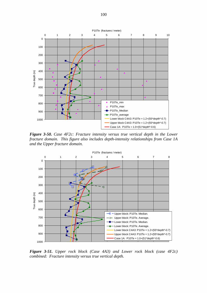
100

Lower rock block: Case 4F2c.

Section length is set to 50m. With Terzaghi correction.

0

100

200

300

400

500

600

700

800

900

1000

0 1 2 3 4 5 6 7 8 9 10

P10Te (fractures / meter)

Tru

e d

ep

th (

m)

P10Te_min

P10Te_max

P10Te_Median

P10Te_average

Lower block C4A3: P10Te = 1.2+(55*depth^-0.7)

Upper block C4A3: P10Te = 1.2+(55*depth^-0.7)

Case 1A: P10Te = 1.0+(51*depth^-0.6)

Figure 3-50. Case 4F2c: Fracture intensity versus true vertical depth in the Lower

fracture domain. This figure also includes depth-intensity relationships from Case 1A

and the Upper fracture domain.

Upper rock block: Case 4A3. Lower rock block: Case 4F2c.

Section length is set to 50m. With Terzaghi correction.

0

100

200

300

400

500

600

700

800

900

1000

0 1 2 3 4 5 6 7 8

P10Te (fractures / meter)

Tru

e d

ep

th (

m)

Upper block: P10Te. Median.

Upper block: P10Te. Average.

Lower block: P10Te. Median.

Lower block: P10Te. Average.

Lower block C4A3: P10Te = 1.2+(55*depth^-0.7)

Upper block C4A3: P10Te = 1.2+(55*depth^-0.7)

Case 1A: P10Te = 1.0+(51*depth^-0.6)

Figure 3-51. Upper rock block (Case 4A3) and Lower rock block (case 4F2c)

combined: Fracture intensity versus true vertical depth.

101

Case 4A3 (Figure 3-48), a direct extension of the orientation model alternative of the

same name, is used to describe the fracture intensity inside the Upper fracture domain.

The fracture intensity analyses show a strong decrease in fracture intensity with

increasing vertical depth, as well as a potential intensity sub-domain. There is a distinct

difference in fracture intensity above and below a TVD of ~ 150 m; whether this

represents the difference between near-surface effects or a true intensity sub-domain is

not known at this time. A clear spike in fracture intensity is also visible at depths of ~

300 m, corresponding to the start of the damage zone surrounding deformation zone

BFZ098. The exponential function describing fracture intensity change with depth for

Case 4A3 was fitted to the observed data so as to produce a non-weighted average

intensity of 2.49 fractures / meter. The resulting equation takes the form of:

L

Te dCCPP 211032

where C1 = 1.2, C2 = 55, L = -0.7, and d = TVD (m) Equation 3-2

A comparison of the results of Case 4A3 versus Case 1A shows a 17% decrease in

average P10Te for the upper rock domain; this suggests that a global (i.e. all domains)

fracture intensity function would be a very poor fit to observational data and would

likely result in the over-estimation of fracture intensities.

The geological DFN model will most likely be implemented in terms of individual

fracture sets, while the parameterization of fracture intensity as a function of depth is for

all fracture sets combined. Therefore, to allow for a set-wise DFN model, it is necessary

to determine the relative fracture set intensities. Relative set intensities from orientation

model alternative case 4A (Table 3-5) are used to break down the total fracture intensity

by set:

SH set: 62%

EW set 18%

NS set 20%

Case 4F2c (Figure 3-50), a direct extension of the orientation model alternative of the

same name, is used to describe the fracture intensity inside the Lower fracture domain.

It is important to note that though the Lower fracture domain extends to the bottom of

the Olkiluoto model volume (TVD of 1000 m); very few boreholes are drilled deeper

than 800 m. Though the Lower fracture domain does show a systematic decrease in

fracture intensity with depth, it is of a far smaller magnitude than in the Upper fracture

domain. In addition, there are several curious patterns noted. First, the average

minimum fracture intensity actually increases with depth from approximately 0.7

fractures per meter at ~ 400 m depth, to almost 1.0 fracture per meter at 800 m depth.

Second, an odd intensity spike is noted between ~ 675 m and 775 m depth; we

tentatively hypothesize that this may be due to modelled deformation zone OL-BFZ099.

However, relatively few boreholes penetrate this deep, and the actual geometric

intersections with this structure are somewhat uncertain; future revisions of the

geological DFN will explore this more detail. The exponential function describing

fracture intensity change with depth for Case 4F2c was fitted to the observed data so as

to produce a non-weighted average intensity of 1.86 fractures / meter. The resulting

equation takes the form of:

102

L

Te dCCPP 211032

where C1 = 1.2, C2 = 55, L = -0.7, and d = TVD (m) Equation 3-3

Note that the best-fit derived exponential function is the same for the Upper and Lower

fracture domains (excluding the Intermediate fracture domain); this implies we can use

the same basic depth versus intensity model to describe both the Upper and Lower

fracture domains (Figure 3-51). Comparisons of the shape of the cumulative frequency

curves (Figure 3-52) show a significant degree of similarity between the Upper and

Lower fracture domains (though not in terms of magnitude). A comparison with Case

1A suggests that Case 4F2c will result in lower average fracture intensities (i.e. closer to

the observed data) by 10% to 16%. Relative set intensities from orientation model

alternative case 4F2 (Table 3-5) are used to break down the total fracture intensity by

set:

SH set: 53%

EW set: 23%

NS set: 24%

Cumulative probability plot.

Distribution of intensity values in upper and lower rock blocks

Upper block: Case 4A3. Lower block: Case 4F2c.

0

10

20

30

40

50

60

70

80

90

100

0 1 2 3 4 5 6 7 8 9 10 11 12

P10Te (1 / meter)

Pro

ba

bility (

%)

Upper block: Case 4A3

Lower block: Case 4F2c

Figure 3-52. Cumulative frequency plot of P10Te in both the Upper (Case 4A3) and

Lower (Case 4F2c) fracture domains.

The Intermediate fracture domain (the rock volume between and around the BFZ098 /

BFZ080 system) has a very limited vertical thickness; fracture intensity within this

domain has not been analyzed as a function of depth. However, representative fracture

intensity properties for this domain have been calculated below in Section 3.3.3.

103

3.3.5 Fracture intensity outside fracture domains

There are a number of boreholes that fall outside the footprint of the ONKALO tunnel

and lie largely outside the extents of the currently-mapped fracture domains, which

themselves are defined largely by the extents of BFZ098 and BFZ080. The boreholes in

question were previously analyzed during the orientation model parameterization, and

are defined by two model alternatives:

Case 4C2: This alternative includes boreholes OL-KR3, OL-KR5, OL-KR6,

OL-KR19, OL-KR20/20B, and OL-KR21. This case evaluates the hypothesis

that fracture intensities to the west-northwest of the mapped limits of BFZ098

should be extremely similar to those mapped in the footwall of BFZ098; and

Case 4D: This case considers block translations / rotations caused by

deformation zone BFZ055; the hypothesis is that fractures on the west-northwest

side (footwall) of BFZ055 will be very similar to Case 4A (affected by

BFZ098), but that fractures on the east-southeast side of BFZ055 will show

changes in the orientations of the fracture set mean poles due to block rotation.

Case 4D utilizes boreholes OL-KR8, OL-KR9, OL-KR23/23B, and OL-KR27.

The results of these analyses are presented below as Table 3-16. Note that these

volumes are not generally treated beyond the analysis stage; future refinements of the

geological DFN model will explore 'filling in' the small volumes between the local

model boundaries and the fracture domains.

Table 3-16. Fracture intensities for rock volumes outside the footprint of the current

(version 1.0) Olkiluoto fracture domains.

Alternative Case

Number of Boreholes

Fracture Sets

P10 P10Te

Average Median Average Median

4C2 6

SH 1.86 1.65 2.33 1.92

NS 0.29 0.26 0.69 0.65

EW 0.30 0.23 0.70 0.66

All 2.45 2.08 4.15 3.51

4D2 5

SH 1.63 1.56 1.91 1.85

NS 0.31 0.32 0.71 0.53

EW 0.37 0.18 0.72 0.50

All 2.32 2.06 3.68 3.29

3.3.6 Fracture intensity at trenches and outcrops

Fracture intensity along surface trenches, and both lineal fracture intensity (P10) and

Terzaghi-compensated fracture intensity (P10Te) were calculated along scanlines. The

trench data was not directly used in the intensity analysis, due to significant questions

about the representativity of the data set. Fracture intensities derived from trench maps

are somewhat at odds with data from both nearby boreholes and the detail-mapped

104

surface outcrops OL-TK10 and OL-TK11. Specifically, measured fracture intensities

are far lower than those measured in the boreholes or on scanlines at OL-TK10 and OL-

TK11. In addition, scanlines have the same problem as boreholes in that even after the

use of Terzaghi-compensation, there is still a strong bias against fractures in certain

orientations (in the case of the trenches, fractures with subhorizontal dips and

subvertical fractures with strikes parallel to the orientation of the scanline). As such, the

fracture intensities for trenches presented in Table 3-17 are used for reference only.

Table 3-17. Fracture intensities recorded along surface trenches at Olkiluoto.

Trench P10 P10Te

OL-TK1 0.91 1.08

OL-TK2 1.00 1.41

OL-TK3 0.91 1.33

OL-TK4 0.79 1.02

OL-TK7 0.74 0.97

OL-TK8 1.42 1.75

OL-TK9 2.59 3.94

OL-TK11 0.99 1.31

OL-TK12 1.18 1.60

OL-TK13 1.19 1.45

Average 1.17 1.59

Median 0.99 1.37

As with the trench data set, the fracture intensity (P21) recorded on the detail-mapped

outcrops was not directly used in the intensity model parameterization. There is no

equivalent to the Terzaghi correction for 2D outcrop trace data; as such, the fracture

outcrop relative set intensities tend to be strongly biased towards vertically- to

subvertically-dipping fracture sets, at the expense of subhorizontally-dipping fractures

(which make up a significant portion of the fracturing at Olkiluoto). This makes it

difficult to use the detail-mapped outcrop data directly in the intensity model

parameterization. Rather, it was included as a key component of the size-intensity

model calibration (Chapter 4), as well as for the estimation of the fracture size model

distribution parameters (scaling exponent and minimum fracture size). Fracture

intensities for the detail-mapped outcrops are presented below in Table 3-18. The

intensity on outcrop OL-TK11 may seem excessively large in comparison to other

trenches, boreholes, and outcrops; this is due to the fact that the outcrop cuts across an

identified deformation zone with a significant transition zone.

Table 3-18. Fracture intensity (P21) recorded on detail-mapped fracture outcrops.

Outcrop ID

Outcrop Area (m

2)

Sum of Trace Lengths (m)

P21 (m/m

2)

Number of Fractures

OL-TK10 799 822.7 1.03 949

OL-TK11 1552 2790.1 1.8 2190

105

3.3.7 Fracture intensity in the ONKALO tunnel

The sidewalls and roof of the ONKALO tunnel have been mapped in detail during

construction; fracture frequency, orientation, host lithology, mineralogy, size, and some

morphological elements (termination styles) have been recorded by Posiva in their

databases. Based on the data available at the writing of this report there are 4233

fractures mapped in the ONKALO tunnel along a section length of approximately 2100

m. The ONKALO tunnel fracture data is a key element of the geological DFN size

model (Section 3.4.2); however, it is not directly used in the fracture intensity modelling

for the same reasons as outcrops OL-TK10 and OL-TK11. In addition, the tunnel

fracture data is also utilized in the calibration of the size-intensity model; matches

observed fracture areal fracture intensity P21 (Figure 3-53) is a key element of the

calibration. In general, the same pattern of decreasing total fracture intensity with

increasing vertical depth was noted in the ONKALO tunnel as in the borehole data.

3.3.8 Fracture intensity model

The following fracture intensity model parameterization is recommended for use in

version 1.0 geological DFN modelling at Olkiluoto:

Upper fracture domain: Assuming a 50 m thick buffer zone between the top of

the ground surface and the beginning of the fracture domain, the recommended

intensity model is: If depth-dependent fracture intensity is desired, Equation 3-2

should be used. If a representative (average) value for the entire fracture domain

is desired, the results of intensity model case 4A3 (Table 3-13) should be used.

Intermediate fracture domain: No depth-dependency suggested; the entire

domain should be treated as a single volume. If only the volume between the

two deformation zones is considered, Case 4F1c (Table 3-14) should be used.

Otherwise, we recommend the use of Case 4F1f (Table 3-14) to describe

intensity within this domain.

Lower fracture domain: For the volume of rock beneath the BFZ098 / BFZ080

deformation zone system, the recommended fracture intensity model is: If depth-

dependent fracture intensity is desired, Equation 3-3 should be used. If a

representative (average) value for the entire fracture domain is desired, the

results of intensity model case 4F2c (Table 3-15) should be used.

106

Onkalo P21(m/m2) at 5 m sections

0

0.5

1

1.5

2

2.5

3

400 600 800 1000 1200 1400 1600 1800 2000

Chainage (m)

P2

1 in

ten

sit

y [

m /m

2]

P21

mean

mean-sigma

Mean+sigma

Median

Figure 3-53. Fracture intensity (P21) measured along the ONKALO tunnel. Lines

represent the arithmetic average fracture intensity and +/- one standard deviation,

based on 5m long tunnel lengths.

3.4 Fracture size model

3.4.1 Model implementation

A description of the methodology used to estimate the distribution of fracture sizes at

Olkiluoto is presented in Section 2.4; this section covers only specific data treatments

and model alternative cases. The primary source of information on fracture sizes are the

traces formed when a fracture intersects a flat or planar surface, such as the walls of a

tunnel or the ground surface. Borehole data is generally not useful, as the diameter of

the core is generally one to two orders of magnitude smaller than the fractures

themselves. The basic methodology for assessing the distribution of fracture sizes at

Olkiluoto is as follows:

1. The walls of the ONKALO access tunnel are approximated as eight planar

traceplanes (Figure 2-5), divided into eight different sections according to length

along the tunnel centreline (Figure 3-54). The length of fractures along each

traceplane is computed, and, for traces crossing multiple trace planes, the

projected surface trace length (and NOT the chord length between start and

endpoint). A minimum trace length of 0.5 m is defined to reduce the effects of

under-sampling on the distribution fit.

2. The analysis in Step 1 is repeated for the detail-mapped fracture outcrops OL-

TK10 and OL-TK11. The main difference between Step 1 and Step 2 is that the

outcrops tend to cover a slightly larger scale (tens of meters) than the tunnels (1-

10 meters) and offer a simplified geometry. A fracture trace recorded in a flat

outcrop represented by a single trace plane can fundamentally be thought of as a

107

random chord through a polygonal fracture in three-space, whereas fractures

along the tunnel walls represent a multi-segment polyline in the plane of a

fracture in three-space.

3. The trace lengths and sampling surface (tunnel, outcrops) geometries are entered

into FracSize (Dershowitz et al. 1998), where the parameters of the parent radius

distribution of the fractures producing the traces are estimated using an iterative

algorithm that combines simulated sampling of a parent fracture radius

distribution with automatic distribution fitting optimization based on conjugate-

gradient or simulated annealing algorithms (Dershowitz et al., 1998). The

analysis is performed for each fracture orientation set. As previously discussed

in the model Assumptions, the only probability distribution tested is Pareto

(power-law). The results of this step are estimates of the radius scaling exponent

(kr), the minimum fracture radius (r0), and the goodness-of-fit statistics between

the ECDF and the CDF. The optimization runs utilized the Simulated Annealing

algorithm, set to minimize the Kolmogorov-Smirnov goodness-of-fit statistic.

FracSize results are presented in Section 3.4.2.

4. As a check against the FracSize distribution fits, trace length scaling analysis is

performed on both detail-mapped surface outcrops. The automatic distribution

fitting methods in FracSize have a tendency to match the tails of the trace length

distribution rather than the full distributional form; this is often true for fracture

traces, where censoring and limited outcrop exposure often only allows for the

non-biased sampling of a very small range of fracture sizes. A second advantage

of tracelength scaling analysis is that if data is available at multiple scales (for

example, trench data at the 1- 10 m scale, combined with high-resolution

LIDAR and ground magnetic surveys at the 10-100 m scale, combined with

regional geophysical lineaments at the 100-1000 m scale), it can, after area-

normalization, be plotted on the same chart to allow for a single continuous size-

scaling relationship calculation. This has been referred to in past geological

DFN reports (Fox et al., 2007; La Pointe et al. 2008) as the 'tectonic continuum'.

Analysis of fracture size data at multiple scales is not performed during the

version 1.0 geological DFN modelling; it is planned for future model revisions.

The trace length scaling analyses are presented in Section 3.4.3.

5. Finally, estimated fracture radius distributions are used in the geological DFN

model calibration, where the links between fracture size, fracture intensity, and

fracture domain are adjusted via Monte-Carlo simulation to produce a final

coupled size-intensity model that best fits the available data at Olkiluoto. The

DFN calibration is discussed in detail in Chapter 5.

108

21001850leg8

18001700leg7

16501400leg6

13501250leg5

1160880leg4

820700leg3

650403leg2

300125leg1

Lower sectionUpper section

21001850leg8

18001700leg7

16501400leg6

13501250leg5

1160880leg4

820700leg3

650403leg2

300125leg1

Lower sectionUpper section

Figure 3-54. Tunnel view with indication of the chainage (upper and lower section) and

the separation into legs (each with a different azimuth) for analyze of trace length

distribution.

An important fact to remember is that fracture size information (at the time of model

completion) was only available for the Upper fracture domain; future ONKALO

mapping efforts are anticipated to penetrate through the Intermediate fracture domains.

The consequence of this lack of data is that the fracture size model parameterization is

strongly controlled by the distribution of fractures in the Upper fracture domain; if

geologic conditions change significantly enough at depth that longer or shorter fractures

are created, the DFN model may not adequately describe their radius distribution.

3.4.2 FracSize analysis results

The results of the FracSize analysis of surface outcrop and ONKALO tunnel and trace

data are presented in Table 3-19 and Table 3-20, respectively. Note that very few of the

tested distributions show statistically-significant degrees of goodness-of-fit; this is a not

uncommon problem when trying to fit distributions to a very small range of numbers (1-

10 m) with a parent dataset with a large degree of censoring and bias. As such,

qualitative judgements of goodness-of-fit are performed by comparing simulated

histograms of trace lengths to field observations in Figure 3-55 through Figure 3-61.

In general, the minimum radius values (r0) calculated on fracture outcrops and in the

ONKALO tunnel are quite similar. This is largely a function of the mapping protocol,

however: the minimum fracture radius fit will be approximately one-half the minimum

trace length measured, if one assumes that trace lengths represent random chords

through circular fractures (La Pointe et al., 2008). There is a large difference between

the radius scaling exponents (kr) fit to data mapped on surface outcrops and data

mapped along the ONKALO tunnel. In particular, the ONKALO tunnel data suggests

scaling exponents that are unusually high. This is largely due to the extremely limited

range of fracture sizes sampled in the tunnel. Past experiences at other hard rock sites in

Sweden have suggested that scaling exponents in the range of 2.0 to 3.5 are generally

appropriate for power-law distributed fracture sizes. As such, the exponents derived

from outcrops are the ones carried forward into the model calibration stage.

Table 3-19. FracSize results for traces on detail-mapped surface outcrops.

Outcrop ID

Fracture Set

Distribution Parameters Simulation Goodness of Fit

r0 kr Number of

Traces Mean

Std. Dev.

Skewness

Kurtosis

K-S %

Confidence χ

2

% Confidence

OL-TK10 SH 0.20 2.20 261 0.63 0.50 2.56 8.86 0.18 3.00 52.00 2.00

OL-TK10 NS 0.15 2.20 327 0.63 0.63 2.84 10.50 0.07 45.00 33.20 0.03

OL-TK10 EW 0.50 2.40 361 0.85 0.74 2.22 6.01 0.08 22.80 39.70 0.03

OL-TK11 SH 0.30 1.80 376 1.68 1.87 2.28 5.28 0.07 24.90 54.60 6.00

OL-TK11 NS 0.25 2.15 727 1.09 1.27 3.47 15.50 0.07 3.62 30.30 0.10

OL-TK11 EW 0.20 2.00 866 1.14 1.43 3.28 12.70 0.06 14.00 29.90 0.40

109

Table 3-20. FracSize results for traces mapped along the ONKALO tunnel.

Tunnel ID

Set ID

Distribution Parameters Mean

Tracelength Standard Dev. Tracelength

Distribution Skewness

Distribution Kurtosis

Goodness of Fit

r0 kr Number of

Traces Sim. Data Sim. Data Sim. Data Sim Data K-S

% Conf.

χ2 % Conf.

Leg2 SH 0.30 3.51 739 1.3 1.81 0.947 2.86 2.32 8.21 10.1 114 0.103 0.0806 71.2 0

Leg3_7 SH 0.26 3.07 558 1.35 1.56 1.25 1.94 4.06 5.91 29.6 52.8 0.066 17.2 36.8 3.42

Leg4_8 SH 0.25 3.00 1381 1.68 1.05 2 1.87 6.58 7.94 57.3 83.5 0.4 0 558 0

Leg5 SH 0.30 3.00 96 1.18 1.26 0.757 1.06 1.51 1.69 3.15 3.08 0.167 13.9 51.6 1.57

leg6 SH 0.19 2.99 1054 1.18 0.927 1.07 1.07 4.46 5.48 41.7 43.8 0.999 0 129 0

Leg2 NS 0.25 4.75 184 0.946 0.947 0.606 1.08 0.826 4.67 0.14 29.3 0.989 0 38 0.387

Leg3_7 NS 0.10 3.72 159 0.559 0.695 0.345 0.564 1.45 1.44 3.11 0.882 0.138 9.53 101 0

Leg4_8 NS 0.29 4.84 1029 0.628 0.704 0.482 0.67 3.68 3.37 25.2 17.6 0.104 0.003 109 0

Leg5 NS 0.49 3.95 129 1.15 1.43 0.717 1.61 1.79 2.77 4.75 9.11 0.202 1.06 52.6 0.064

leg6 NS 0.22 3.75 492 0.641 0.917 0.72 1.73 5.47 5.79 44.8 39.9 0.081 7.74 37.1 2.33

Leg2 EW 0.34 3.11 343 1.26 1.54 1.52 2.28 4.63 3.92 28.6 17.8 0.088 14.5 59.7 0.045

Leg3_7 EW 0.20 3.48 240 0.734 0.845 0.624 1.23 4.47 8.24 36.6 94.2 0.104 14.8 18.7 13.1

Leg4_8 EW 0.20 3.00 1234 0.959 0.978 0.911 1.75 4.48 11.8 33.1 218 0.997 0 41.1 0.055

Leg5 EW 0.30 2.50 124 1.72 1.14 2.76 1.15 5.5 2.51 38.3 6.94 0.226 0.359 35.4 0.352

leg6 EW 0.11 2.59 433 0.836 1.3 0.623 2.33 2.31 4.92 8.23 30.4 0.938 0 71.3 0

110

111

Figure 3-55. Histograms of simulated (FracSize) versus observed trace length

distribution on outcrop OL-TK11.

112

Figure 3-56. Histograms of simulated (FracSize) versus observed trace length

distribution on outcrop OL-TK10.

113

Figure 3-57. Histogram of observed versus simulated trace lengths along Leg 2 of the

ONKALO tunnel.

114

Figure 3-58. Histograms of simulated and observed trace length for Legs 3 and 7

combined along the ONKALO tunnel.

115

Figure 3-59. Histogram of observed versus simulated trace lengths along Leg 5 of the

ONKALO tunnel.

116

Figure 3-60. Histogram matching of trace length for Leg 6.

117

Figure 3-61. Histograms of simulated versus observed fracture traces along Legs 4 and

8 (combined) of the ONKALO tunnel.

118

3.4.3 Tracelength scaling analysis on surface outcrops

The goal of the tracelength scaling analysis is to provide a check of the parent radius

distribution parameters derived from the FracSize simulation. In addition, should data at

additional scales be available, the tracelength scaling method provides for the

development of a size model at multiple scales simultaneously. The disadvantage,

however, is that for this method to work, we must assume that fracture traces (and

therefore fracture radii) are scale-invariant and follow a power-law distribution (Section

2.4.1); it is not possible to test other distributions of fracture size.

The methodology of this analysis is described in detail in Section 2.4.3; the cumulative

number for each fracture trace, either as a function of fracture set or of all sets combined

is first calculated. The resulting cumulative number is divided by the area of the target

outcrop so as to normalize for different sampling areas. This is not strictly necessary

when working with data at a single scale, but it is done anyway for completeness. The

resulting area-normalized complementary cumulative numbers are plotted on log-log

axes as a function of trace length. The slope of the fracture trace length scaling exponent

(kt) is estimated by manually fitting a straight line to the straight portions of the data; the

curves at either end of the trace length series represent systematic under-sampling or

censoring due to mapping resolution limits or the size of the outcrop relative to the size

of the fracture traces. The radius scaling exponent kr is calculated from the trace length

scaling exponent kt using Equation 2-7.

The results of the tracelength scaling analysis are presented graphically as Figure 3-62

through Figure 3-64, with summary parameters contained in Table 3-21. For both

outcrops, the fracture radius exponents estimated from tracelength scaling analysis are

fairly similar to those from the FracSize analysis; the FracSize numbers are generally

slightly lower due to the tendency of the automated fitting algorithms to over-emphasize

the shorter tracelengths. The relatively long straight sections on all charts suggest that,

at least at the 1 - 10 m scale, fracture radii are well-described by a power law, even if

there is some uncertainty in the actual scaling exponent. The only anomaly is with the

NS fracture set on outcrop OL-TK11, where there is a significant discrepancy between

the FracSize and tracelength scaling fits; the tracelength scaling fit will be used as the

base input to model calibration for this set.

Table 3-21. Summary of tracelength scaling analysis and comparison to FracSize

results for surface outcrops OL-TK10 and OL-TK11.

Outcrop Fracture Set kt kr kr from FracSize

OL-TK10 NS 1.31 2.31 2.20

OL-TK10 EW 1.33 2.33 2.20

OL-TK10 SH 1.24 2.24 2.40

OL-TK10 All 1.29 2.29 n/a

OL-TK11 NS 1.45 2.45 1.80

OL-TK11 EW 1.21 2.21 2.15

OL-TK11 SH 1.27 2.27 2.00

OL-TK11 All 1.41 2.41 n/a

119

CNP: OL-TK10 Sets

0.0001

0.001

0.01

0.1

1

10

0.01 0.1 1 10 100

Tracelength (m)

Are

a-n

orm

alized

cu

mu

lati

ve n

um

ber

NS Set

EW Set

SH Set

NS Set kt = 1.31

EW Set kt = 1.33

SH Set kt = 1.24

Figure 3-62. Area-normalized complementary cumulative number plots for fracture sets

on outcrop OL-TK10. The slope of the best-fit line is the trace length scaling exponent

(kt) which is one less than the fracture radius scaling exponent (kr).

CNP: OL-TK11 Sets

0.0001

0.001

0.01

0.1

1

10

0.01 0.1 1 10 100

Tracelength (m)

Are

a-n

orm

ali

ze

d c

um

ula

tiv

e n

um

be

r

NS Set

EW Set

SH Set

NS Set kt = 1.45

EW Set kt = 1.21

SH Set kt = 1.27

Figure 3-63. Area-normalized complementary cumulative number plots for fracture sets

on outcrop OL-TK11. The slope of the best-fit line is the trace length scaling exponent

(kt) which is one less than the fracture radius scaling exponent (kr).

120

CNP: OL-TK10 / OL-TK11 All Sets Combined

0.0001

0.001

0.01

0.1

1

10

0.01 0.1 1 10 100

Tracelength (m)

Are

a-n

orm

alized

cu

mu

lati

ve n

um

ber

OL-TK10 All Sets

OL-TK11 All Sets

OL-TK10 kt = 1.29

OL-TK11 kt = 1.41

Figure 3-64. Area-normalized complementary cumulative number plots for all fracture

sets combined on outcrops OL-TK10 and OL-TK11. The slope of the best-fit line is the

trace length scaling exponent (kt) which is one less than the fracture radius scaling

exponent (kr).

3.5 Fracture spatial model

As described in the modelling methodology and assumptions (Section 2.1), several

assumptions have been made regarding the spatial arrangement of fractures at Olkiluoto.

First, the base assumption is that fracture intensity scales in a Euclidean fashion with

increasing size; fundamentally, this means as you double the area sampled, the number

of fractures doubles. This hypothesis is evaluated through the use of the fractal mass

dimension (Section 2.6.1; c.f. Feder, 1988) calculated for fracture traces on detail-

mapped surface outcrops.

Second, we assume that, in the absence of strong geologic correlations to lithology,

bedrock alteration, or existing geologic structures that fracture centres follow a Poisson

point process in three dimensions. The Poisson point process describes a system of

single events which occur randomly in 'time' with no memory or correlation to past

events (Cressie, 1993). The Poisson point process has been found at other hard rock

sites in the Nordic countries (Fox et al. 2007, La Pointe et al., 2008) to be a reasonable

approximation for the location of fractures from minimum scales of 10 to 30 meters up

to scales of tens of kilometres. This assumption is tested using Baecher analysis

(Baecher et al., 1978) of the fractal box dimension (Feder, 1988) calculated on detail-

mapped fracture outcrops.

Finally, the degree of lithologic and depth control on fracture intensity is also a

component of the spatial model. This was evaluated in detail in Section 3.3. Future

revisions of the geological DFN model will focus on a better quantification of the

121

spatial variability of fracturing, including geostatistical evaluation of the ONKLAO

tunnel and the calculation of the mass and box dimensions for cored boreholes.

The results of the fractal mass dimension analyses are presented below in Figure 3-65

and Figure 3-66. All analyses were completed using GeoFractal (La Pointe et al., 2000).

The mass dimension was calculated using 150 random centres inside a guard area

approximately the extents of each outcrop; the fractal mass dimension is calculated from

the intersection of fracture traces with 21 embedded concentric circles at each random

centre. If fracture intensity scaling is Euclidean, the mass dimension should be

approximately 2.0. For outcrop OL-TK10, the mass dimension is approximately 2.2,

suggesting that at outcrop scales (1 - 10m) the outcrop trace data is slightly fractal. For

outcrop OL-TK11, the mass dimension is approximately 2.05; given the uncertainty in

both the data collection and quality of fracture trace maps at Olkiluoto, this is 'close

enough' to 2.0 to be considered Euclidean scaling.

140.

20.

40.

60.

80.

100.

120.

0.

Co

un

t F

rac

ture

-Fra

ctu

re I

nte

rs.

0. 2. 4. 6. 8. 10. 12. 14.

R a d iu s (m )

Mass Fractal Analysis Power Law function: Least Squares method

Exponent = 2.18775 Coefficient = 0.385645

SSQ (sum of sq. errors) = 191291

Std.Deviaton Error = 8.4234

Figure 3-65. Mass dimension analysis for outcrop OL-TK10. The slope of the red line

represents the fractal mass dimension, fit using non-linear least squares.

122

M ass Fractal A nalysis

3.

1.

2.

0.

Co

un

t F

rac

ture

-Fra

ctu

re I

nte

rs.

(•1

0

0. 5. 10. 15. 20. 25.Radius

Power Law function: Least Squares method

Exponent = 2.05243 Coefficient = 4.74328 SSQ (sum of sq. errors) = 1.00667e+008

Std.Deviaton Error = 183.366

Figure 3-66. Mass dimension analysis for outcrop OL-TK11. The slope of the red line

represents the fractal mass dimension, fit using non-linear least squares.

The results of the fractal box dimension and Baecher analysis are presented below in

Figure 3-68 through Figure 3-72. All analyses were completed using geoFractal. The

box dimension was calculated using fracture-cell intersections (OL-TK10) and fractures

centers (OL-TK11) on a 2.5 m x 2.5 m grid applied to each outcrop. The grid extents are

somewhat less than the extents of the outcrop, to minimize the number of empty grid

cells. Goodness-of-fit is evaluated through the Kolmogorov-Smirnov test against the

box count CDF. Both the Baecher analysis results (Figure 3-68) and the outcrop

tracemap (Figure 3-67) for OL-TK10 suggests that, at this outcrop, the fracture pattern

is not at all well-described as random in space. A generalized Gamma distribution

(Figure 3-69) appears to be a much better fit. Outcrop OL-TK11 is a much better fit to

the Poisson distribution (Figure 3-71), and is beginning to look like what we would

expect from a Baecher model for fracture centers. The generalized Gamma distribution

(Figure 3-72) is still a better fit, however.

123

6792400.

6792360.

6792370.

6792380.

6792390.

6792350.

1526598. 1526608. 1526618. 1526628. 1526638. 1526648. 1526658. 1526668. 1526678.

OL-TK10 - Fracture Trace

No

rth

ings (

m)

Eastings (m)

6792400.

6792360.

6792370.

6792380.

6792390.

6792350.

1526598. 1526608. 1526618. 1526628. 1526638. 1526648. 1526658. 1526668. 1526678.

OL-TK10 - Fracture Trace

No

rth

ings (

m)

Eastings (m)

Figure 3-67. Outcrop OL-TK10. Note the strong clustering of smaller fractures around

larger fractures on this outcrop; a Poissonian fracture location model may not be

appropriate, if the mapped features are correct.

1.

0.2

0.4

0.6

0.8

0.

Pe

rce

ntile

0. 50. 100. 150.

Amt.of Fracture-Cell Intersections

Baecher Analysis (CDF)

Poisson distribution: Parameters selected by user Poisson mean = 50.4375 K-S statistic = 0.416532

Significance level = 2.77841e-015

1.

0.2

0.4

0.6

0.8

0.

Pe

rce

ntile

0. 50. 100. 150.

Amt.of Fracture-Cell Intersections

Baecher Analysis (CDF)

Poisson distribution: Parameters selected by user Poisson mean = 50.4375 K-S statistic = 0.416532

Significance level = 2.77841e-015

Poisson distribution: Parameters selected by user Poisson mean = 50.4375 K-S statistic = 0.416532

Significance level = 2.77841e-015

Figure 3-68. Baecher analysis for outcrop OL-TK10. The red line represents the

empirical CDF of the best-fit Poisson distribution for fracture centers. The Poisson

distribution is not a particularly good fit.

124

1.

0.2

0.4

0.6

0.8

0.

Perc

entile

0. 50. 100. 150.

Amt.of Fracture-Cell Intersections

Baecher Analysis (CDF)

Gamma distribution: Moments fitted

Alpha = 2.25878 Beta = 22.3295

K-S statistic = 0.0966055

Significance level = 0.316305

1.

0.2

0.4

0.6

0.8

0.

Perc

entile

0. 50. 100. 150.

Amt.of Fracture-Cell Intersections

Baecher Analysis (CDF)

Gamma distribution: Moments fitted

Alpha = 2.25878 Beta = 22.3295

K-S statistic = 0.0966055

Significance level = 0.316305

Gamma distribution: Moments fitted

Alpha = 2.25878 Beta = 22.3295

K-S statistic = 0.0966055

Significance level = 0.316305

Figure 3-69. Baecher analysis for outcrop OL-TK10 fit to a generalized Gamma

distribution. This is a much better fit.

6792060.

6792010.

6792020.

6792030.

6792040.

6792050.

6792000.

1525884. 1525894. 1525904. 1525914. 1525924. 1525934. 1525944. 1525954. 1525964. 1525974. 1525984.

OL-TK11 - Fracture Trace

Nort

hin

gs (

m)

Eastings (m)

6792060.

6792010.

6792020.

6792030.

6792040.

6792050.

6792000.

1525884. 1525894. 1525904. 1525914. 1525924. 1525934. 1525944. 1525954. 1525964. 1525974. 1525984.

OL-TK11 - Fracture Trace

Nort

hin

gs (

m)

Eastings (m)

Figure 3-70. Outcrop OL-TK11. This outcrop shows a significantly more Poissonian

spatial pattern, though the presence of a large deformation zone along the eastern edge

of the outcrop has an adverse affect on model statistics.

125

1.

0.2

0.4

0.6

0.8

0.

Perc

entile

0. 5. 10. 15. 20.

Amt.of Fracture Centers in Cell

Baecher Analysis (CDF)

Poisson distribution: MLE fit

Poisson mean = 5.38816

K-S statistic = 0.168472

Significance level = 4.98374e-008

1.

0.2

0.4

0.6

0.8

0.

Perc

entile

0. 5. 10. 15. 20.

Amt.of Fracture Centers in Cell

Baecher Analysis (CDF)

Poisson distribution: MLE fit

Poisson mean = 5.38816

K-S statistic = 0.168472

Significance level = 4.98374e-008

Poisson distribution: MLE fit

Poisson mean = 5.38816

K-S statistic = 0.168472

Significance level = 4.98374e-008

Figure 3-71. Baecher analysis for outcrop OL-TK11 fit to the Poisson distribution.

Though the Poisson distribution goodness-of-fit is significantly better on OL-TK11 than

for outcrop OL-TK10, the Poissonian model is not able to completely capture all spatial

variability at the outcrop scale.

1.

0.2

0.4

0.6

0.8

0.

Pe

rce

ntile

0. 5. 10. 15. 20.

Amt.of Fracture Centers in Cell

Baecher Analysis (CDF)

Gamma distribution: Moments fitted

Alpha = 1.90367 Beta = 2.8304

K-S statistic = 0.124288

Significance level = 0.00014548

1.

0.2

0.4

0.6

0.8

0.

Pe

rce

ntile

0. 5. 10. 15. 20.

Amt.of Fracture Centers in Cell

Baecher Analysis (CDF)

Gamma distribution: Moments fitted

Alpha = 1.90367 Beta = 2.8304

K-S statistic = 0.124288

Significance level = 0.00014548

Gamma distribution: Moments fitted

Alpha = 1.90367 Beta = 2.8304

K-S statistic = 0.124288

Significance level = 0.00014548

Figure 3-72. Baecher analysis for outcrop OL-TK11 fit to a generalized Gamma

distribution. The Gamma distribution still proves a better description of the location of

fractures in space.

126

127

4 MODEL CALIBRATION AND VERIFICATION

4.1 Calibration strategy

The final step in the development of the version 1.0 Olkiluoto geological DFN model is

the calibration of the fracture size and fracture intensity models to best reproduce the

conditions seen in-situ. Calibration and parameterization are an iterative process:

During parameterization we postulate hypotheses about how the fracture system works

and calculate distribution parameters, while during calibration the distribution

parameters are tested to see if they can truly reproduce in-situ conditions, and, if not, to

make changes. This is especially important when using a coupled size-intensity model

such as the power law, where the size and intensity are parameterized separately, but in

the model implementation are fundamentally dependent on each other.

It is difficult to develop a single model calibrated to all different sources of fracture

data. The calibration efforts for the version 1.0 geological DFN are designed to find the

best-fit parameters for size and intensity for three model scenarios:

Model 1: Fracture orientation and fracture intensity are based predominantly on

borehole data from the Upper fracture domain. The median value of fracture P32

(P10Te) from Case 4A3 was adopted as a reference value; P32 was fixed while the

remaining size / intensity parameters were adjusted to achieve the best-possible

fit between modelled and observed fractures;

Model 2: The goal of this scenario was to produce a better match in terms of P21

on the detail-mapped fracture outcrops (OL-TK10 and OL-TK11). The P32

intensity of the subhorizontal (SH) fracture set in the cored borehole array was

adjusted so as to reduce the difference between simulated/observed cored

borehole P10 and simulated/observed outcrop P21; and

Model 3: This scenario is based on a late review of fracture size data from the

ONKALO tunnel received in early 2008. This model adjusts the minimum

radius (r0) parameter of the power-law distribution to produce a slightly better fit

to observed tunnel P21 intensity.

Note that the spatial model is included in the model calibration; future geological DFN

revisions will include tests of the performance of both models during the validation

stage. The DFN parameters have been adjusted (calibrated) in a way that the established

models produce a reasonable fit to the measured intensity of the outcrop traces, the

intensity of the tunnel traces and the borehole intensity. The calibration is performed

through Monte-Carlo simulation of 20 realizations of each specific DFN scenario within

a 50 m x 100 m x 100 m simulation volume. Calibration is performed by comparing

simulated results on two simulated traceplanes and six simulated boreholes. Boreholes

have (randomly) been assigned similar trends and plunges to boreholes drilled near the

ONKALO tunnel. Aggregate statistics are then taken from the Monte-Carlo results, and

the mean simulation values compared to the mean of the measured data at Olkiluoto to

determine which model provides the most 'reasonable' fit. A reasonable fit is defined as:

128

a quantitative analysis of the differences between the simulated and measured

values (i.e. goodness of fit statistic, absolute and standard error, etc.); and

a qualitative interpretation taking into account the uncertainty ranges of the

measured data, considering each kind of data (borehole, outcrop, and tunnel).

4.2 Outcrop simulations

Table 4-1 presents the results of the model calibration, in terms of fracture intensity P21

measured on outcrop. A key problem is that the intensity of OL-TK10 and OL-TK11

are distinctly different, even though they reside in the same fracture domain. As such, it

is extremely difficult to come up with a model that simultaneously fits both outcrops. If

the intensity of both outcrops is averaged, Model 3 performs the best at reproducing

what is seen at Olkiluoto. Figure 4-1 illustrates the calibration results graphically as a

box and whisker plot; it shows that though the overall differences between the three

model scenarios are small in terms of the average fracture intensity, Models 1 and 3 are

far less variable in terms of spikes and lulls in fracture intensity.

Table 4-1. Comparison of simulated and measured P21 during calibration efforts. This

table presents the results of 20 simulations.

Scenario

Outcrop

P21

Mean Std. Dev. Min. Max. Measured

Model 1 OL-TK10 1.676 0.118 1.498 1.984 1.80

Model 1 OL-TK11 1.602 0.072 1.443 1.703 1.03

Model 2 OL-TK10 1.531 1.534 1.252 2.237 1.80

Model 2 OL-TK11 1.523 1.323 1.334 2.119 1.03

Model 3 OL-TK10 1.472 0.076 1.364 1.629 1.80

Model 3 OL-TK11 1.393 0.041 1.325 1.471 1.03

One of the best ways of evaluating the performance of the various model scenarios is

through the use of cumulative number plots (CNP) of fracture traces. The shape of the

CNP plots (Figure 4-2 through Figure 4-4), including the departure from power-law

size-scaling (when the data follows a curve instead of a straight line in log-log space),

make a qualitative assessment of model performance much easier. The CNP plots show

that none of the chosen model scenarios are a particularly good fit to OL-TK10, while

Model 1 is a very good fit to outcrop OL-TK11. As previously mentioned, Model 3 is

the best-fit to the average of both outcrops, but is still unable to truly capture the P21

fracture intensity exhibited on OL-TK11. In the future, effort should be spent on

determining if there are significant geological or morphological differences between

OL-TK10 and OL-TK11 that could explain the differences in fracture intensity between

the two outcrops.

129

P21 (m/m2)

0

0.5

1

1.5

2

2.5

TK10 model

1

TK11 model

1

TK10 model

2

TK11 model

2

TK10 model

3

TK11 model

3

outcrops -simulated

P2

1

Min P21

Max P21

Mean P21

Figure 4-1. Comparison of simulated and measured P21 values on outcrops OL-TK10

(yellow line) and OL-TK11 (green line).

Outcrops CNP - Cumulated Normalized Plot model 1

0.001

0.01

0.1

1

10

0.1 1 10 100

Trace length (m)

Are

a n

orm

aliz

ed c

um

ula

tive n

um

ber

TK10 measured

TK11 measured

kt = 1.63

TK11 simulated

TK10 simulated

Figure 4-2. Outcrop CNP plot for Model 1, showing measured and simulated trace

length distributions. The value 'kt' represents the trace length scaling exponent, which is

one less than the radius scaling exponent.

130

Comparisons of the distributions of simulated and measured fracture trace lengths for

the outcrops are shown in Figure 4-5 and Figure 4-6. These histograms were produced

from one realization of scenario Model 2. They show that the best fit between the

simulation parameters and the outcrop are data are for traces longer than 1.5 m. If we

take into account that actual traces shorter than about one meter or larger than about five

meters are probably strongly censored, Model 2 produces a reasonable 'middle ground'

fit to the two actual (measured) size distributions (OL-TK10 and OL-TK11).

Outcrops CNP - Cumulated Normalized Plot model 2

0.001

0.01

0.1

1

10

0.1 1 10 100

Trace length (m)

Are

a n

orm

alize

d c

um

ula

tive

nu

mb

er

TK10 measured

TK11 measured

kt = 1.63

TK11 simulated

TK10 simulated

Figure 4-3. Outcrop CNP plot for Model 2, showing measured and simulated trace

length distributions.

131

Model 3 - Normalized cumulative plot of trace length

0.001

0.01

0.1

1

10

0.1 1 10 100trace length (m)

no

rma

lize

d b

y a

rea

co

un

t

TK11 measured

TK11Simulated

TK10 Simulated

TK10 measured

Figure 4-4. Outcrop CNP plot for Model 3, showing measured and simulated trace

length distributions.

Histogram outcrop TK10 - Model 2

0

50

100

150

200

250

300

350

400

450

500

0.5

1.5

2.5

3.5

4.5

5.5

6.5

7.5

8.5

9.5

10.5

11.5

More

Trace length (m)

Fre

qu

en

cy

Tk10_measured

Simulated

Figure 4-5. Histogram of measured (blue) and simulated (red) fracture traces on

outcrop OL-TK10 from one realization of Model 2.

132

Histogram outcrop TK11 - Model 2

0

100

200

300

400

500

600

700

800

900

0.5

1.5

2.5

3.5

4.5

5.5

6.5

7.5

8.5

9.5

10.5

11.5

More

Trace length (m)

Fre

qu

en

cy

TK11 measured

Simulated

Figure 4-6. Histogram of measured (blue) and simulated (red) fracture traces on

outcrop OL-TK11 from one realization of Model 2.

An important step in the DFN model calibration involves the qualitative analysis of the

simulated trace patterns produced by the geological DFN model. The chosen size-

intensity parameterization may produce a reasonable statistical match, but the geologists

and engineers using the model must have confidence that the trace pattern ultimately

produced is reasonable; i.e. the model 'looks' like reality. Simulated trace patterns are

compared to observational data in Figure 4-7 and Figure 4-8; in general, Models 2 and 3

appear to produce trace pattern most similar to those observed on outcrop OL-TK11.

However, none of the scenarios do a particularly good job of reproducing trace intensity

patterns on outcrop OL-TK10; it is possible that this outcrop is not representative of the

Upper fracture domain.

133

Model 3 Model 2

Model 1

measure

d

Figure 4-7. Actual and simulated trace maps for outcrop TK11. The top figure presents

the simulated traces for models 2 and 3 as well as for model 1. The measured traces are

presented in the lower figure. The simulated traces were produced by one realization of

the DFN-model.

134

Model 3 Model 2

Model 1

measured

Figure 4-8. Actual and simulated trace maps for outcrop TK10. The top figure presents

the simulated traces for models 2 and 3 as well as for model 1. The measured traces are

presented in the lower figure. The simulated traces were produced by one realization of

the DFN-model.

135

Finally, three additional cumulative number plots (Figure 4-9 through Figure 4-11)

document the comparison of simulated to observed fracture set intensities to determine

if the relative set intensities noted in the Upper fracture domain can be reproduced.

These figures describe results for OL-TK11 from one iteration of the 20 runs used in the

model calibration. A perfect fit is not expected, as the lack of a correction for

orientation bias for the outcrops implies that the SH set will not match the relative

intensities seen in the boreholes. However, the general patterns for the NS and EW

subvertical sets should be relatively unaffected by orientation bias.

It is interesting to note that the fit of the sub-horizontal fracture set is better for Model 2

and 3 than for Model 1, especially for traces longer than 1 m. For the sub-vertical sets,

the fit of Model 2 is not significantly better than the fits achieved with Model 1. The

reason for the better fit produced by Model 2 for the sub-horizontal set is that for Model

2 and 3 the intensity of the sub-horizontal fracture set was reduced compared to Model

1, with a corresponding increase in the radius scaling exponent. The result is that the

size distribution becomes slanted towards smaller fractures, which fall underneath the

0.5m truncation threshold, further reducing intensities. A model with a smaller value of

the fracture intensity of the sub-horizontal fracture set will produce a better match to the

surface data, as the surface data demonstrates a smaller intensity of sub-horizontal

fractures than the borehole data. For Model 3, the NS vertical set has a different slope

(radius scaling exponent) than the measured data; this stems from the use of the

FracSize tunnel results over the outcrop trace length scaling results when establishing

Model 3.

TK11 model 1 - CNP by set

0.001

0.01

0.1

1

0.1 1 10 100

Trace length (m)

Are

a n

orm

aliz

ed c

um

ula

tive n

um

ber

TK11 EW

TK11 NS

TK11 SH

TK11_Sim_SH

TK11_Sim_NS

TK11_Sim_EW

Figure 4-9. CNP plot of simulated and measured traces as a function of fracture

orientation set on outcrop OL-TK11. The simulated data in this chart is taken from

scenario Model 1.

136

TK11 model 2 -CNP by set

0.001

0.01

0.1

1

0.1 1 10 100

Trace length (m)

Are

a n

orm

aliz

ed c

um

ula

tive n

um

ber

TK11 EW

TK11 NS

TK11 SH

TK11_sim_SH

TK11_sim_NS

TK11_sim_EW

Figure 4-10. CNP plot of simulated and measured traces as a function of fracture

orientation set on outcrop OL-TK11. The simulated data in this chart is taken from

scenario Model 2.

TK11 Model 3 - CNP by set

0.001

0.01

0.1

1

0.1 1 10 100

trace length

norm

aliz

ed b

y a

rea c

ount

TK11 EW

TK11 NS

TK11 SH

kt = 1.62

TK11_simEW

Tk11_sim_NS

TK11_sim_SH

Figure 4-11. CNP plot of simulated and measured traces as a function of fracture

orientation set on outcrop OL-TK11. The simulated data in this chart is taken from

scenario Model 3.

137

4.3 ONKALO tunnel simulations

The second step in the calibration of the version 1.0 Olkiluoto geological DFN model

was to find the parameters that best matched the fracture trace observations recorded

along the ONKALO tunnel. Fracture intensity (P21) along the tunnel has been computed

for 5-m long strips on each of the eight sampling traceplanes, and is presented in Figure

3-53. Comparison plots of each of the three model scenarios are presented as Figure 4-

12 through Figure 4-14, with summary statistics given in Table 4-2.

A closer look at the results suggests that Models 2 and 3 produce a P21 intensity that is

closer to the measured values than Model 1. However, in all of the scenarios, the current

DFN model overestimates average fracture intensity by 50% - 200%, depending on

depth. Part of this is due to the fact that the calibration simulations did not make use of a

depth-dependent intensity relationship, but instead focused on matching the size and

intensity in the first 1000 m of the ONKALO tunnel. The inclusion of depth-

dependency will significantly improve the model performance at tunnel lengths greater

than 1000m. We also suspect that the mapping protocol in the ONKALO tunnel

significantly undercounts smaller fractures; future iterations of the geological DFN

models will attempt to quantify the degree to which the tunnel walls are different from

the cored borehole and outcrop mapping protocols.

Comparing model 1

simulated (dashed) and measured P21 at Onkalo

0

0.2

0.4

0.6

0.8

1

1.2

1.4

1.6

1.8

2

400 600 800 1000 1200 1400 1600 1800 2000

Chainage (m)

P2

1 in

ten

sity [m

/m

2]

mean

mean-sigma

Mean+sigma

Median

Mean model 1

Min model 1

Max model 1

Figure 4-12. Comparison of average, maximum, and minimum simulated and observed

P21 computed for 5m strips along the ONKALO tunnel for scenario Model 1.

138

Table 4-2. Average simulation summary statistics for ONKALO tunnel calibration.

Scenario P21 (m/m

2)

Mean Minimum Maximum

Model 1 1.78 1.55 2.10

Model 2 1.44 1.17 1.78

Model 3 1.44 1.27 1.65

Comparing model 2

simulated (dashed) and measured P21 at Onkalo

0

0.2

0.4

0.6

0.8

1

1.2

1.4

1.6

1.8

400 600 800 1000 1200 1400 1600 1800 2000

Chainage (m)

P2

1 in

ten

sity [m

/m

2]

mean

mean-sigma

Mean+sigma

Median

Mean model 2

Min model 2

Max model 2

Figure 4-13. Comparison of average, maximum, and minimum simulated and observed

P21 computed for 5m strips along the ONKALO tunnel for scenario Model 2.

Comparing model 3 simulated and measured P21 at Onkalo

0

0.2

0.4

0.6

0.8

1

1.2

1.4

1.6

1.8

400 600 800 1000 1200 1400 1600 1800 2000

Chainage (m)

P21 in

tensity

[m

/m

2]

mean

mean-sigma

Mean+sigma

Median

Mean model3

Min Model 3

Max Model 3

Figure 4-14. Comparison of average, maximum, and minimum simulated and observed

P21 computed for 5m strips along the ONKALO tunnel for scenario Model 3.

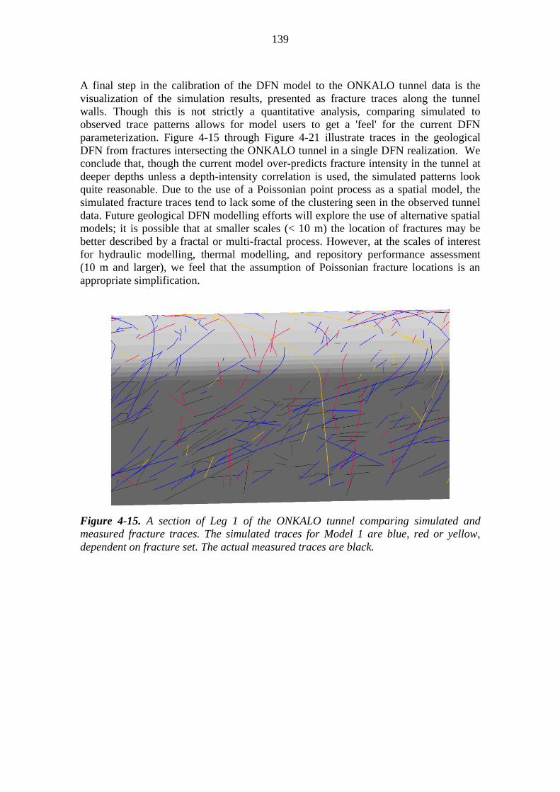
139

A final step in the calibration of the DFN model to the ONKALO tunnel data is the

visualization of the simulation results, presented as fracture traces along the tunnel

walls. Though this is not strictly a quantitative analysis, comparing simulated to

observed trace patterns allows for model users to get a 'feel' for the current DFN

parameterization. Figure 4-15 through Figure 4-21 illustrate traces in the geological

DFN from fractures intersecting the ONKALO tunnel in a single DFN realization. We

conclude that, though the current model over-predicts fracture intensity in the tunnel at

deeper depths unless a depth-intensity correlation is used, the simulated patterns look

quite reasonable. Due to the use of a Poissonian point process as a spatial model, the

simulated fracture traces tend to lack some of the clustering seen in the observed tunnel

data. Future geological DFN modelling efforts will explore the use of alternative spatial

models; it is possible that at smaller scales (< 10 m) the location of fractures may be

better described by a fractal or multi-fractal process. However, at the scales of interest

for hydraulic modelling, thermal modelling, and repository performance assessment

(10 m and larger), we feel that the assumption of Poissonian fracture locations is an

appropriate simplification.

Figure 4-15. A section of Leg 1 of the ONKALO tunnel comparing simulated and

measured fracture traces. The simulated traces for Model 1 are blue, red or yellow,

dependent on fracture set. The actual measured traces are black.

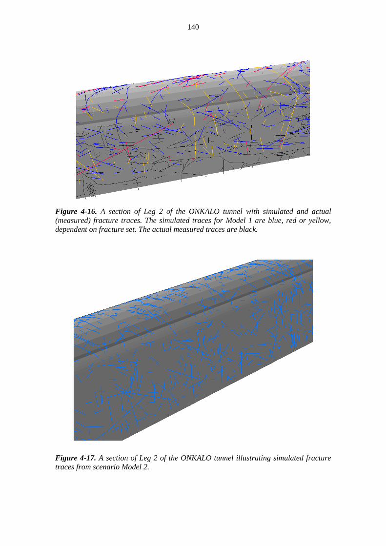
140

Figure 4-16. A section of Leg 2 of the ONKALO tunnel with simulated and actual

(measured) fracture traces. The simulated traces for Model 1 are blue, red or yellow,

dependent on fracture set. The actual measured traces are black.

Figure 4-17. A section of Leg 2 of the ONKALO tunnel illustrating simulated fracture

traces from scenario Model 2.

141

Figure 4-18. A section of leg 2with simulated fracture traces for Model 3

Figure 4-19. A section of Leg 3 of the ONKALO tunnel with simulated and measured

fracture traces. The simulated traces for scenario Model 1 are blue, red or yellow,

dependent on fracture set. The actual measured traces are black.

142

Figure 4-20. Another section of Leg 3 of the ONKALO with simulated fracture traces

from scenario Model 2.

Figure 4-21. A section of Leg 3 of the ONKALO tunnel with simulated fracture traces

from scenario Model 3.

143

4.4 Borehole simulations

The calibration of the geological DFN model to borehole data is by far the most

important process in the model parameterization. As much of the geological DFN

(fracture orientation, fracture domains, fracture depth-dependency, and fracture

intensity) is based primarily on data acquired from boreholes, if the final model

parameterization cannot come close to reproducing observed reality, the DFN model is

fundamentally flawed. The borehole calibration process was conducted in the same way

as both the outcrop and ONKALO tunnel calibrations: 20 Monte-Carlo realizations of

each of the three primary scenarios were produced. The calibration is based on the

comparison of average simulated fracture P10 to observed fracture P10. Note that in these

calibrations, no depth-dependency is used. Rather, we are focused on matching the total

fracture intensity across the entire model volume (similar to orientation model

alternative Case 1A). Use of depth-dependent fracture intensity models will

significantly improve performance in the upper 200-300m of the model.

Calibration results are presented below as Figure 4-22 through Figure 4-24. Model 1

produces the best fit to measured data in terms of measured and simulated average

fracture P10, while Models 2 and 3 tend to underestimate fracture intensity in the

boreholes. There are two potential causes of this. First, Model 2 and Model 3 emphasize

matching the surface outcrop and ONKALO tunnel fracture intensities, respectively.

Second of all, it is highly likely that the minimum size (r0) derived from fracture

outcrops and tunnel walls is too small; because of the high resolution of fracture core

logs and extensive areal coverage, some, if not many of the fractures seen in drill cores

are likely to be too small to have been recorded by other sampling methods. Past

geological DFN models in Sweden (Fox et al., 2007; La Pointe et al. 2008) have

suggested that though minimum radius of 0.4 - 0.9 are appropriate to describe outcrop

fracturing, it is generally necessary to decrease the minimum radius to close to 2x the

radius of the borehole (~ 0.07 - 0.1 m) to simultaneously match outcrop and borehole

intensity. Future geological DFN refinements will explore the discrepancy between the

fracture intensity recorded in cored boreholes, along the ONKALO tunnel, and in pilot

blast holes drilled as the ONKALO tunnel is advanced.

144

Using Bore holes: 8, 26, 28, 30, 35, 36

0

100

200

300

400

500

600

0 1 2 3 4 5 6

Model 1 - P10 (fractures / meter)

Tru

e d

ep

th (

m)

P10min

P10max

P10(Median)

P10average

Average_simulated

Max_sim

Min_sim

Figure 4-22. Simulated and measured P10 value calculated along 50 m depth intervals

for scenario Model 1.

Using Bore holes: 8, 26, 28, 30, 35, 36

0

100

200

300

400

500

600

0 1 2 3 4 5 6

Model 2 - P10 (fractures / meter)

Tru

e d

ep

th (

m)

P10min

P10max

P10(Median)

P10average

Average_simulated

Max_sim

Min_sim

Figure 4-23. Simulated and measured P10 value calculated along 50 m depth intervals

for scenario Model 2.

145

Using Bore holes: 8, 26, 28, 30, 35, 36

0

100

200

300

400

500

600

0 1 2 3 4 5 6

Model 3 - P10 (fractures / meter)

Tru

e d

ep

th (

m)

P10min

P10max

P10(Median)

P10average

Average_simulated

Max_sim

Min_sim

Figure 4-24. Simulated and measured P10 value calculated along 50 m depth intervals

for scenario Model 3.

4.5 Calibration results and recommendations

The results of the geological DFN model parameterization are fundamentally a simple

quantification of uncertainty. They illustrate the rather large probability space (and

corresponding uncertainty) within which the version 1.0 geological DFN model exists.

Future model revisions, combined with new and revised data, will help to reduce some

of the uncertainty in our understanding of the fracture system at Olkiluoto. As a 'first-

draft' of a geological DFN model for the Olkiluoto site, the current model

parameterization will be useful for answering basic hypotheses about fracturing inside

the local model volume, and is a starting point for downstream modelling teams

(Hydrogeology).

The DFN model calibration (summarized below in Table 4-3) suggests that the

following model parameters should be used to simulate fractures at Olkiluoto:

Fracture intensity should be modelled as depth-dependent;

Due to the lack of information from the Intermediate and Lower fracture

domains, the fracture size model has to be based on the Upper fracture domain;

and

Fracture orientation is a function of fracture domain.

146

Table 4-3. Calibration simulation results and recommended model parameters for

geological DFN simulation at Olkiluoto.

Parameter Set / Units Model 1 Model 2 Model 3

Fracture Intensity

P32 SH Set (m2/m

3) 1.43 1.15 1.15

P32 EW Set (m2/m

3) 0.41 0.41 0.41

P32 NS Set (m2/m

3) 0.46 0.46 0.46

Fracture Size

SH Set r0 0.35 0.35 0.45

SH Set kr 2.50 2.70 2.80

EW Set r0 0.25 0.25 0.45

EW Set kr 2.30 2.30 2.70

NS Set r0 0.35 0.35 0.45

NS Set kr 2.20 2.20 3.60

Fracture

Orientation

SH Set (Trend, Plunge, κ) 320 65 8.2 320 65 8.2 320 65 8.2

NS Set (Trend, Plunge, κ) 358 4 8.1 358 4 8.1 358 4 8.1

EW Set (Trend, Plunge, κ) 268 8 8.1 268 8 8.1 268 8 8.1

147

5 CONCLUSIONS AND RECOMMENDATIONS

5.1 Version 1.0 DFN model summary

DFN Orientation Model

It was determined that describing fracture orientation as a function of fracture domain

was the most consistent and straightforward method for characterizing fracture sets at

Olkiluoto. The orientation model can be described as a function of fracture domain as

follows:

For the Upper fracture domain, the orientation model from Case 4A (all

boreholes above BFZ098) is recommended. This domain is dominated by

shallowly-dipping fractures that strike northeast and dip to southeast; the

fractures in this domain appear to generally follow the orientation of the bedrock

foliation.

For the Intermediate fracture domain, the orientation model from Case 4F1 is

used. This alternative model case utilizes the average mean pole vectors for all

borehole sections between deformation zones BFZ098 and BFZ080. Fracture

orientations and relative set intensities in this domain are thought to be strongly

influenced by the surrounding deformation zones. The Intermediate zone is

notable for a decrease in the relative intensity of the northeast striking

subhorizontal set, and the presence of an intense northwest-striking, northeast

dipping secondary subhorizontal set.

The Lower fracture domain is best represented using orientation model case

4F2, which includes fractures from boreholes beneath a 100m zone of influence

in the footwall underneath BFZ098. This domain is characterized by a

pronounced change in subhorizontal fracture strike; the majority of fractures in

this domain strike east-west and dip to the south at moderate angles (30° – 50°).

Table 5-1. Recommended fracture orientation model. All values assume univariate

Fisher hemispherical probability distributions.

Fracture Domain

EW pole set NS pole Set SH pole Set

Trend (°) Plunge

(°) κ Trend (°)

Plunge (°)

κ Trend

(°) Plunge

(°) κ

Upper 277 5 8.1 350 5 8.1 313 62 8.2

Intermediate 81 0 5.5 181 2 5.9 273 72 6.2

Lower 269 7 6.6 358 7 7 328 60 7

DFN Size Model

Though presented in this report as separate model elements, the version 1.1 Olkiluoto

DFN model is fundamentally a coupled size-intensity model; parameters for one aspect

148

of the model (such as the size, or the P10Te / P32 intensity) cannot be changed without a

corresponding change in other parameters. This is a key feature of modelling fracture

size as a power law. The size-intensity model contains three variables:

kr: The fracture radius scaling exponent;

r0 / rmin: The minimum sized fracture (in terms of equivalent radius) treated by

the size model. r0 represents the minimum value of the PDF, while rmin

represents a minimum size cut-off that is generally larger than r0; and

P32: The volumetric fracture intensity, calculated from the Terzaghi-corrected

cored borehole P10 (P10TE). There are no alternative size-intensity models based

on different interpretations or calculations of P32.

Table 5-2. Recommended fracture size model. All values assume a power-law (Pareto)

probability distribution for fracture equivalent radius.

Fracture Set

Model 1 Model 2 Model 3

kr r0 kr r0 kr r0

SH 2.50 0.35 2.70 0.35 2.80 0.45

NS 2.20 0.35 2.20 0.35 3.60 0.45

EW 2.30 0.25 2.30 0.25 2.70 0.45

DFN Intensity Model

An analysis of borehole fracture frequency suggests that, at Olkiluoto, fracture intensity

is correlated to depth below the ground surface. Table 4-3 presents average observed

borehole fracture intensities, as a function of elevation below the ground surface. There

is a clear decrease in the intensity of all fracture sets with increasing depth; the largest

contrast is in a narrow (100 m thick) zone near the ground surface. We suspect that the

increased fracture intensity near the ground surface represents a combination of post-

glacial unloading and the effects of stress-release at a free interface. Based on the results

of the intensity analysis and the model validation / calibration efforts, the recommended

intensity models for DFN simulations at Olkiluoto are:

Upper fracture domain: If the volume below an elevation of -50 m is to be

simulated as a whole, Case 4A3 presented below in Table 4-5 is the

recommended P32 intensity model. Relative fracture set intensity should be

modelled according to the following percentages: SH Set = 62% NS Set = 20%

EW Set = 18%. If depth-dependency of fracturing is desired, Equation 3-2

should be used;

Intermediate fracture domain: For the volume of rock between deformation

zones BFZ098 and BFZ080, Case 4F1c (Table 4-5) is the recommended P32

intensity model. We do not recommend attempting depth-dependent fracture

intensity modelling in this domain; and

149

Lower fracture domain: For the volume of rock in the footwall of deformation

zone BFZ080, Case 4F2c (Table 4-5) is the recommended P32 intensity model.

Relative fracture set intensity should be modelled according to the following

percentages: SH Set = 55%, NS Set = 24%, EW Set = 21%. If depth-dependency

of fracturing is desired, Equation 3-3 should be used.

DFN Spatial Model

Based on the limited spatial analysis of fractures exposed on surface outcrops, a Poisson

point process model is suggested for the location of fracture centres in three-space.

Fracture size-intensity scaling should be simulated as Euclidean. Weak lithologic

correlations to fracture intensity were noted; however, their magnitudes are far smaller

than the differences between fracture domains and as a function of depth. Therefore, we

recommend that fracture orientation and intensity should be correlated solely to depth

and fracture domain. No fracture termination relationships have been evaluated.

5.2 DFN model uncertainties

A formal evaluation and quantification of DFN model uncertainties is not included in

the scope of work for the version 1.0 geological DFN; we highly recommend including

time and budget for such an activity in future site work. Nevertheless, we can come to

some basic conclusions about the relative magnitudes of different model uncertainties

based on past experiences at similar hard-rock sites in Sweden and the results of the

various analyses completed during DFN model parameterization. First, however, it is

useful to present a linguistic framework for understanding uncertainty.

In general, uncertainty can be divided into two basic types: aleatoric uncertainty and

epistemic uncertainty. Aleatoric uncertainty represents the uncertainty inherent in the

modelling process (data collection, evaluation, simulation approximations, etc) and is

fundamentally irreducible; the inclusion of additional data or processes cannot eliminate

aleatoric uncertainties. The best example of aleatoric uncertainty is the classic 'coin-

flip'; the probability of getting the desired outcome (heads or tales) is always 0.5 and

will not be changed by the inclusion of additional data. Epistemic uncertainty is

described as an external uncertainty whose magnitude can be reduced by the inclusion

of additional data or knowledge about rates, processes, boundary conditions, etc. An

example of epistemic uncertainty is predicting the winner of a horse race: initially, the

probability of each one of the horses to win is equal. However, with knowledge of the

past performance, response to atmospheric and ground surface conditions, the

experience of the jockey, and the relative strength of the horse with respect to the length

of the race, the epistemic component of the uncertainty regarding the prediction of the

winner can be reduced.

Most of the aleatoric uncertainties at Olkiluoto centre around the fact that it will never

be possible to completely characterize every square meter of the proposed repository

volume; if fracture properties are at least partially dependent on volumetric properties

(stress state, lithology, and alteration); there will always be an irreducible component of

uncertainty. However, many of the uncertainties inherent in geological modelling do fall

in to the epistemic class. We further subdivide these uncertainties into three general

domains, based on work done for the Total System Performance Analysis (TSPA) at the

150

Yucca Mountain Project (YMP) high-level spent fuel repository in the United States

(SAIC, 2001):

1. Conceptual Model uncertainties arise from an incomplete understanding of the

physical or chemical processes being modelled. The conceptual model

uncertainties for the version 1.0 Olkiluoto geological DFN include:

Whether the spatial model for fractures at Olkiluoto is truly Poissonian;

Whether the fracture size model (r0, kr) is independent or dependent on

fracture domain. As a coupled size-intensity model based on calibration

of P32 to existing in-situ conditions, completely different model fits are

possible if one changes this hypothesis;

Whether a univariate Fisher distribution is adequate to characterize

fracture orientations at Olkiluoto; and

Whether fracture intensity scaling is truly Euclidean, or whether a fractal,

multi-fractal, or Gaussian intensity scaling process would be more

appropriate.

2. Representational Model uncertainties arise from the approximations,

simplifications, and numerical treatment of inputs, operations, and outputs

necessary to transform the conceptual model(s) into forms suitable for numerical

simulation.

Treatment of fractures as planar polygons with no real thickness; and

Quantification of the minimum size of fractures based on fits to data

(i.e. deriving r0 analytically based on P32).

3. Parameter uncertainties arise from imperfect knowledge of the system being

modelled, errors and omissions in measurements, or due to limited and / or non-

representative data. Parameter uncertainties for the version 1.0 Olkiluoto

geological DFN include:

Uncertainty in the size-intensity scaling exponent (kr), based on different

data sources;

Uncertainty in the size model due to the lack of data at multiple scales

and the (somewhat) extreme censoring affect on both sides (very small

and very large fractures) of the distribution;

Uncertainty in the quality of orientation measurements; and

Uncertainty in the amount, coverage, and representativity of fracture data

collected along the ONKALO tunnel.

Note that though conceptual models tend to dominate both the number and magnitude

of uncertainties in a static DFN model, far more attention is generally paid to

quantifying parameter uncertainties, which, in our experience, are generally second-

order in term of the magnitude of their effects on model performance. Experiences at

similar project sites (Forsmark and Laxemar in Sweden, Sudbury in Canada) have

suggested that fracture size is by far the most uncertain parameter in a geological DFN,

151

and one that has the largest affect on system performance. In a coupled size-intensity

model such as the one postulated in this report, the variability of fracture intensity also

plays a large, first-order role. Fracture orientations and spatial locations tend to play a

lesser role, provided that deformation zones are not included in the statistical model.

Finally, there are a number of additional questions arising from the analysis of fracture

data during the development of the geological DFN model. These questions should be

addressed during future modelling work, and include:

What is the true spatial variability of bedrock foliation and ductile structures;

how much does the foliation truly control fracturing?

What is our understanding of the state of in-situ rock stress at Olkiluoto, and

what kind of spatial / compositional / depth variability is seen?

Is the depth-fracture intensity correlation the strongest relationship we see, or

can fracturing be linked to additional rock properties?

What are the extents of the transition zones (if they exist) around the

deformation zones at Olkiluoto? The inclusion or exclusion of fractures inside

deformation zones has a (potentially) large effect on the DFN parameterization.

5.3 Conclusions and recommendations for future work

In general, the division of the rock mass at Olkiluoto into fracture domains

characterized by relatively homogeneous fracture domains has gone a long ways

towards improving the understanding of the brittle fracture system. The version 1.0

geological DFN model is a good 'first-step' towards a characterization of fracturing in

the rock mass at Olkiluoto, and the linking of fracture intensity to vertical depth will be

a key result going forwards.

As version 1.1 of the DFN represents an interim modelling product, additional work can

and should be done to further understand rock fracturing at Olkiluoto. Specifically, the

following tasks are recommended for the next stage of geological modelling:

Evaluation of alternative spatial models (fractal clustering, geostatistical, etc);

Evaluation of fracture intensity scaling (Euclidean, fractal, or discontinuous)

across multiple observational scales;

Better coupling of fracture domains and DFN parameters to bedrock geology,

regional structure, tectonics, and stress history, if possible;

Inclusion of deformation zones and lineaments in size modelling along the lines

of the ‘tectonic continuum’ concept utilized by SKB at Forsmark and Laxemar

in Sweden (Fox et al. 2007, La Pointe et al. 2005);

Evaluation of alternative orientation spherical probability distributions to

describe fracture orientations at Olkiluoto. It is possible that a ‘girdle’

distribution (Bingham) might better reproduce the orientation variability;

152

Additional analysis of spatial variability of intensity with respect to the

occurrence and volume of subordinate rock types, as well as additional

quantification of the variability within a given domain;

Analysis and quantification of fractures inside the zone of influence of

deformation zones. These fractures are likely to be of importance for

hydrogeological and transport modelling in repository performance assessment

(PA);

Additional verification, and potentially validation, of the geological DFN model

through stochastic simulation;

Explicit quantification of uncertainties in the geological DFN model;

Integration of additional feedback from other modelling teams and disciplines;

and

Feedback from the hydrogeological and rock mechanics teams are especially

desired.

153

REFERENCES

Baecher, G., Lanney, N., and Einstein, H., 1977, Statistical Description of Rock

Properties and Sampling: Proceedings of the 18th

U.S. Symposium on Rock

Mechanics, p. 5C1-1 to 5C1-8

Baecher, G., and Lanney, N., 1978, Trace length biases in joint surveys: Proceedings

of the 19th

U.S. Symposium on Rock Mechanics, v. 1, p. 56-65.

Bechtel-SAIC, 2001, Uncertainty Analyses and Strategy: Report SAIC011481M4

Revision 00,

Caine, J., Evans, J., and Forster C., 1996, Fault zone architecture and permeability

structure: Geology v. 24, no. 11, p. 1025-1028.

Call, R.D., Savely, J.P., and Nicholas, D.E., 1976, Estimation of joint set

characteristics from surface mapping data: Proceedings of the 17th

U.S. Symposium

on Rock Mechanics, p. 2B2-1 to 2B2-9.

Chilès, J-P., and de Marsily, G., 1993, Stochastic models of fracture systems and their

use in flow and transport modelling, in Bear J., Tsang, C-F. and de Marsily, G., Flow

and Contaminant Transport In Fractured Rock: Academic Press Inc. ISBN 0-12-

083980-6.

Cressie, N., 1993, Statistics for spatial data, revised edition: New York, USA, John

Wiley and Sons. ISBN 0-471-00255-0.

Cruden, D., and Ranalli, G., 1977, Length distribution of strike-slip faults and the

process of breakage in continental crust: Canadian Journal of Earth Sciences (Journal

Canadien des Sciences de la Terre), v. 14 no.3, p. 508–510.

Davis, J., 2002, Statistics and Data Analysis in Geology, Third Edition: New York,

USA, John Wiley and Sons. ISBN 978-0471172758

Davy, P., Darcel, C., Bour, O., Munier, R., de Dreuzy J-R., 2006, A note on the

angular correction applied to fracture intensity profiles along drill core: Journal of

Geophysical Research, v. 111 no. B11408.

Dershowitz, W., 1984, Rock Joint Systems: Doctoral dissertation, Massachusetts

Institute of Technology, Cambridge, MA, USA.

Dershowitz, W., Lee, G., Geier, J., Foxford, T., La Pointe, P., Thomas, A., 1998,

FRACMAN Interactive discrete feature data analysis, geometric modelling and

exploration simulation, User documentation, version 2.6: Redmond, Washington,

USA, Golder Associates, Inc.

Epstein, H., 1947, The mathematical description of certain breakage mechanisms

leading to the logarithmico-normal distribution: Journal of the Franklin Institute, v.

244, p. 471-477.

154

Feder, J., 1988, Fractals: New York, USA, Plenum Press. ISBN 0-306-42851-2.

Fisher, R. A., 1953, Dispersion on a sphere: Proc. R. Soc. A217, 295-305.

Fisher, N. I., Lewis, T., Embleton, B. J. J., 1987, Statistical analysis of spherical data:

Cambridge, UK, Cambridge University Press. ISBN 0-521-45699-1.

Fleuty, M. J., 1964, Tectonic slides: Geological Magazine, v. 101 no. 5, p. 453 – 456.

Fox, A., La Pointe, P., Hermanson, J., and Öhman, J., 2007, Statistical geological

discrete fracture network model – Forsmark modeling stage 2.2: Report R-07-46,

Stockholm, Sweden, Svensk Kärnbränslehantering AB.

Hammah, R. E., and Curran, J. H., 1998, Fuzzy Cluster Algorithm for the Automatic

Identification of Joint Sets: International Journal of Rock Mechanics and Mining

Science, v. 35 no. 7, p. 889-905.

Hammah, R. E., and Curran, J. H., 1999, On distance measures for the Fuzzy K-

means algorithm for joint data: Rock Mechanics and Rock Engineering, v. 32 no. 1, p.

1-27.

Hermanson, J., Forssberg, O., Fox, A., La Pointe, P., 2005, Statistical model of

fractures and deformation zones. Preliminary site description, Laxemar subarea,

version 1.2: Report R-05-45, Stockholm, Sweden, Svensk Kärnbränslehantering AB.

Hofrichter, J., and Winkler, G., 2003, Statistical analysis for the hydrogeological

evaluation of the fracture networks in hard rocks: RMZ – Materials and

Geoenvironment, v. 50 no. 1, p. 145-148.

Holmén, J., Outters, N., 2002, Theoretical Study of Rock Mass Investigation

Efficiency: Report TR-02-21, Stockholm, Sweden, Svensk Kärnbränslehantering AB.

Kagan, Y.Y., 1997, Seismic moment-frequency relation for shallow earthquakes;

regionalcomparison: Journal of Geophysical Research, B - Solid Earth and Planets, v.

102 n. 2, p. 2835–2852.

Kamb, W., 1959, Ice petrofabric observations from Blue Glacier, Washington, in

relation to theory and experiments: Journal of Geophysical Research, v. 64, p. 1891-

1919.

Korhonen, K., Kuivamäki, A., Paananen, M., Paulamäki, S., 2005. Lineament

Interpretation of the Olkiluoto Area: Working Report 2005-34, Olkiluoto, Finland,

Posiva OY.

La Pointe, P., Wallmann, P., and Dershowitz, W., 1993, Stochastic estimation of

fracture size from simulated sampling: International Journal of Rock Mechanics,

Mining Sciences. & Geomechanics Abstracts, v. 30, p. 1611-1617.

155

La Pointe, P., Burago, A., Lee, K., and Dershowitz, B., 2000, geoFractal:

Geostatistical and Fractal Analysis for Spatial Data, User Manual version 1.0,

Redmond, Washington, Golder Associates Inc.

La Pointe, P., 2002, Derivation of parent fracture population statistics from trace

length measurements for fractal fracture populations: International Journal of Rock

Mechanics and Mining Sciences, v. 39, p. 381-388.

La Pointe, P., and Hermanson, J., 2005, Statistical model of fractures and deformation

zones. Preliminary site description, Simpevarp subarea, version 1.2 (SDM Simpevarp

1.2 DFN model): Report R-05-28, Stockholm, Sweden, Svensk Kärnbränslehantering

AB.

Mandelbrot, B., 1982, The fractal geometry of nature: San Francisco, California,

USA, Freeman Press.

Mardia, K.V., 1972, Statistics of directional data, London, Academic Press.

Mattila, J., Aaltonen, I., Kemppainen, K., Wikström, L., Paananen, M., Paulamäki, S.,

Front, K., Gehör, S., Kärki, A., and Ahokas, T., 2008, Geological Model of the

Olkiluoto Site, Version 1.0: Working Report 2007-92, Olkiluoto, Finland, Posiva Oy.

Milnes, A. G., Hudson, J., Aaltonen, I., Wikström, L., 2006. Foliation: Geological

Background, Rock Mechanics Significance, and Preliminary Investigations at

Olkiluoto. Working Report 2006-03. Posiva Oy, Eurajoki.

Mauldon, M., and Mauldon, J. G., 1997, Fracture sampling on a cylinder; from

scanlines to boreholes and tunnels: Rock Mechanics and Rock Engineering, v. 30, no.

3, p. 129-144.

Munier, R., 2004, Statistical analysis of fracture data adapted for modelling Discrete

Fracture Networks-Version 2: Report R-04-66, Stockholm, Sweden, Svensk

Kärnbränslehantering AB.

Munier, R., and Stigsson, M., 2007, Implementation of uncertainties in borehole

geometries and geological orientation data in Sicada: Report R-07-19, Stockholm,

Sweden, Svensk Kärnbränslehantering AB.

Munier, R., Stenberg, L., Stanfors, R., Milnes, A-G., Hermanson, J., and Triumf , C-

A., 2003, Geological Site Descriptive Model; A strategy for the model development

during site investigations: Report R-03-07, Stockholm, Sweden, Svensk

Kärnbränslehantering AB.

Munier, R., 2004, Statistical analysis of fracture data, adapted for modelling discrete

fracture networks-Version 2: Report R-04-66, Stockholm, Sweden, Svensk

Kärnbränslehantering AB.

NIST, 2007a. Kolmogorov-Smirnov Goodness-of-Fit Test, Chapter 1.3.5.16,

NIST/SEMATECH e-Handbook of Statistical Methods, National Institute of

156

Standards and Technology, United States Department of Commerce, Washington

D.C., USA.

http://www.itl.nist.gov/div898/handbook/eda/section3/eda35g.htm

Last accessed 20090612.

NIST, 2007b. Gamma distribution, Chapter 1.3.6.11, NIST/SEMATECH e-Handbook

of Statistical Methods, National Institute of Standards and Technology, United States

Department of Commerce, Washington D.C., USA. Last accessed 20090612.

http://www.itl.nist.gov/div898/handbook/eda/section3/eda366b.htm

Pareto, V., 1897, Cours d'économie politique professé à l'université de Lausanne, 3

volumes, 1896-1897.

Peacock, D.C.P., Harris, S., and Mauldon, M., 2003, Use of curved scanlines and

boreholes to predict fracture frequencies: Journal of Structural Geology, v. 25, p. 109-

119.

Press, W., Flannery, B., Teukolsky, S., Vetterling, W., 1992, Numerical Recipes in C:

The Art of Scientific Computing: Cambridge, UK, Cambridge University Press.

Priest, S. D., and Hudson, J. A., 1981, Estimation of discontinuity spacings and trace

length using scanline surveys: International Journal of Rock Mechanics and Mining

Science and Geomechanical Abstracts, vol. 18, p. 183 – 197.

Priest, S. D., 1993, Discontinuity Analysis for Rock Engineering: New York, USA,

Chapman & Hall Inc (now CRC Press). ISBN 0-412-47600-2.

Paulamäki, S., Paananen, M., Gehör, S., Kärki, A., Front, K., Aaltonen, I., Ahokas, T.,

Kemppainen, K., Mattila, J., and Wikström, L., 2006, Geological model of the

Olkiluoto site version 0: Working report 2006-37, Olkiluoto, Finland, Posiva Oy.

Rohrbaugh, M., Dunne, W., and Mauldon, M., 2002, Estimating fracture trace

intensity, density, and mean length using circular scan lines and windows: AAPG

Bulletin, v. 86 no. 12, p. 2089-2104.

Schaeben, H., 1984, A new cluster algorithm for orientation data: Journal of the

International Association for Mathematical Geology, v. 16 no. 2, p. 139-153.

Shanley, R. J., and Mahtab, M. A., 1976, Delineation and analysis of clusters in

orientation data: Journal of the International Association for Mathematical Geology,

v. 8 no. 1, p. 9-23.

Terzhagi, R. D., 1965, Sources of error in joint surveys: Geotechnique, v. 15, p. 287-

304.

Wahlgren, C-H., Curtis, P., Hermanson, J., Forssberg, O., Öhman, J., Fox, A., La

Pointe, P., Drake, H., Triumf, C-A., Mattsson, H., Thunehed, H., Juhlin, C., 2008,

Geology Laxemar Site descriptive modelling, SDM-Site Laxemar: Report R-08-54,

Stockholm, Sweden, Svensk Kärnbränslehantering AB.

157

Wang, X., 2005, Stereological Interpretation of Rock Fracture Traces on Borehole

Walls and Other Cylindrical Surfaces: Doctoral Dissertation, Virginia Polytechnic

Institute and State University, Virginia, USA.

Watson, G. S., 1960, More significance tests on the sphere: Biometrika, v. 47, p. 87-

91.

Woodcock, N., and Naylor, M., 1983, Randomness testing in three-dimensional

orientation data: Journal of Structural Geology, v. 5, p. 539-548.

Yow, J. L., 1987, Technical Note: Blind zones in the acquisition of discontinuity

orientation data: International Journal of Rock Mechanics and Mining Science and

Geomechanics Abstracts, v. 24 no. 5, p. 317-318.

158