Rheologica Acta Rheol Acta 32:311-321 (1993)

Generating line spectra from experimental responses. Part h Relaxation modulus and creep compliance

I. Emri 1 and N.W. Tschoegl 2

University of Ljubljana, Ljubljana, Slovenia 2California Institute of Technology, Pasadena, California, USA

Abstract: We describe a recursive computer algorithm which generates line spec- tra from relaxation modulus or creep compliance data without producing negative spectrum lines. We apply the algorithm here to data read from mathematical models for the relaxation modulus. Since these data were thus free of the usual experimental error, we could use a relatively simple form of the basic algorithm that is applicable also to smoothed data. The spectra faithfully reproduced the input functions and may serve for data storage as well as for predicting other experimental responses.

Key words." Creep compliance - line spectrum - relaxation modulus - relaxa- tion spectrum - retardation spectrum

Introduction

In the response of a linearly viscoelastic material to a strain excitation, the relaxation spectrum, H(z) , contains complete information on the time-dependent part of the response. In the response to a stress excita- tion it is the retardation spectrum, L(z) , which con- tains the information. In either case the total response then consists of the appropriate viscoelastic constants (such as the equilibrium modulus, or the glass com- pliance and the steady-flow fluidity), in addition to the integral over the spectrum multiplied by a kernel function characteristic of the type of excitation chosen to elicit the response. I f this is a strain or a stress as a step function of time, the kernel is the ex- ponential function, exp ( - t/r), and the result of the integration is the relaxation modulus in the first case, and the creep compliance in the second case. Thus, once the spectrum and the viscoelastic constants are known, it is possible, in theory, to generate the response to any desired type of excitation.

The spectrum itself is not accessible by direct ex- periment (Tschoegl, 1989; pp. 157-158) . From a mathematical model of a response curve it can often be calculated exactly (Tschoegl, 1989; p. 196). How- ever, f rom experimental data the spectrum is necessarily obtained as an approximation to the un- known ' t rue ' spectrum whose existence is but assum- ed. Commonly, one obtains approximations to the

spectra f rom experimental data by numerical or graphical differentiation or by the use of finite dif- ference calculus (Tschoegl, 1989; Sect. 4.2 and Sect. 4.3). These methods are based on the canonical (i.e., integral) representations (Tschoegl, 1989; p. 160) of the experimental response and yield sets of values sampled f rom the approximations to the con- tinuous spectra.

Another approach is based on the representation of the experimental response by discrete canonical models (Tschoegl, 1989; pp. 134, 160) leading to distributions of line spectra. Once a line spectrum is available, any response curve within the same representational group (i,e., within relaxation or creep behavior) can be generated readily. Line spectra obtained f rom time-dependent and frequency-depen- dent data can easily be combined into a single spec- t rum covering a wide range of respondance times. Thus, a line spectrum is also an excellent means for the storage of experimental data.

Determination of a line spectrum is essentially a curve fitting procedure. We must distinguish between two possible fits. The first will produce the best mathematical fit, but is bound to produce some negative spectrum lines. Such lines are physically unacceptable and can create havoc in any interconver- sion, particularly when converting between relaxation and retardation behavior. The second fit eliminates all negative spectrum lines (zero lines are physically

312 Rheologica Acta, Vol. 32, No. 3 (1993)

acceptable). Such a fit will not produce the best fit to the datum points, but will more closely approach the intrinsic material property. No line spectrum - pro- duced by whatever method - is ever the true spec- trum. This necessarily remains unknown. Further- more, no such spectrum is unique because its exact nature depends on the parameters introduced to ob- tain it. The success of a spectral distribution is mea- sured by comparing the original experimental data with those reconstructed from the distribution.

Unfortunately, attempts to develop suitable methods for obtaining well-determined line spectra from which the input function can be faithfully reconstructred, have hitherto not met with un- qualified success. Among the better known older methods of this type (Tschoegl, 1989; Sect. 3.6, p. 136ff) are Procedure X of Tobolsky and Murakami (1959), the Collocation method of Schapery (1962), and an extension of it by Cost and Becker (1970) call- ed the Multidata method. The two last named require matrix inversion. Both are likely to generate negative modulus or compliance values in portions of the line spectrum. If positive lines appropriately compensate such negative lines, the occurrence of the latter may not unduly affect the reconstruction of the input curve. However, this compensation depends on the exact choice of the input parameters. This makes it virtually impossible to generate any other experimen- tal responses from a "compensated" spectrum with any degree of confidence.

Due undoubtedly to the easy availability of suffi- ciently powerful computers, the last several years have seen an increase in interest in methods for com- puting spectral distributions. The literature now con- tains several more recent papers devoted to this sub- ject (Baumgaertel and Winter, 1989; Elster and Honercamp, 1991, 1992; Elster, Honercamp and Weese, 1991; Honercamp, 1989; Honercamp and Weese, 1989; Janzen and Scanlan, 1993; Kamath and Mackley, 1989; Laun, 1986, Orbey and Dealy, 1991). We wish to make our own contribution to it by offer- ing a recursive computer algorithm specifically designed to avoid negative spectrum lines. The meth- od of Baumgaertel and Winter (1989), e.g., also avoids negative spectrum lines, albeit at the expense of reducing the density of the lines. However, we refrain here from a detailed review o f earlier papers by other authors because an extensive comparison is currently in preparation (Tschoegl and Emri, to be submitted). We do point out, however, that our algorithm does not require matrix inversion and that - in contrast to all other methods of which we are aware - it computes each spectrum line utilizing only

well-defined subsets of the complete set of experimen- tal data. The choice of these subsets is governed by the form of the kernel functions in the canonical representations of the experimental response func- tions. Consequently, there exist several forms of the basic algorithm, one for each kernel function. Our algorithms (we use the singular or the plural as appro- priate) thus avoid potential sources of instabilities in the computations.

In this paper, we introduce the algorithm in the form in which it is applied to simulated step response curves, i.e., to continuous mathematical functions having all the characteristics of the relaxation modulus or the creep compliance demanded by the theory of linear viscoelasticity (Tschoegl, 1989; Sect. 6.1, pp. 314-326). A companion paper (Tschoegl and Emri 1993 a) deals with the determination of the spectra from simulated storage and loss functions. A third paper (Tschoegl and Emri, 1992) takes up the problem of interconverting between relaxation and retardation line spectra. In these three papers, we apply the algorithm to data sets obtained by sampling continuous theoretical curves which - being free of experimental error - are either monotone non-in- creasing [e.g. G (t), J ' (co)], monotone non-decreasing [e.g. G'(og), J(t)], or both [e.g. G"(co), J"(co)]. This simplifies the algorithm, the presentation of its basic nature, and the demonstration of its power. A fourth paper [Emri and Tschoegl, 1993b) deals with the ap- plication to experimental data exhibiting considerable scatter as is usual, e.g., when the time scale has been extended through time-temperature superposition. In that paper, we propose a modification of the algorithm in which the relative rather than the ab- solute error forms the basis of the criterion for exiting from an iteration. It must be pointed out, however, that the simpler forms of the algorithm that we report in this and in the companion paper are by no means restricted to simulated data. They can, e.g., be ap- plied successfully to smoothed data (Emri und Tschoegl, 1993 b). Smoothing of the data with an effi- cient smoothing tool such as the cubic spline function (Emri and Tschoegl, 1993b) is almost universally beneficial. We have, however, applied the simpler forms of the algorithm described here with excellent results also to unsmoothed data that contained moderate experimental error.

Theoretical

The form of the basic algorithm we discuss here determines a line spectrum from a step response func- tion such as G(t) or J(t). It obtains the strength of the

Emri and Tschoegl, Generating line spectra from experimental responses 313

line associated with each of a set of predetermined respondance times (relaxation or retardation times) recursively. Although it does not require that the respondance times be equally spaced, we use equal- spacing for convenience.

To understand how the algorithm does its work, let us first consider the reverse calculation, i.e., the re- construction of the relaxation modulus from a discrete distribution of spectrum lines. Let this distri- bution, for simplicity's sake, consist of four lines, equally spaced on the logarithmic time scale, and let

gi(t) = giexp ( - t /r ,) {i = 1,2,3,4} (1)

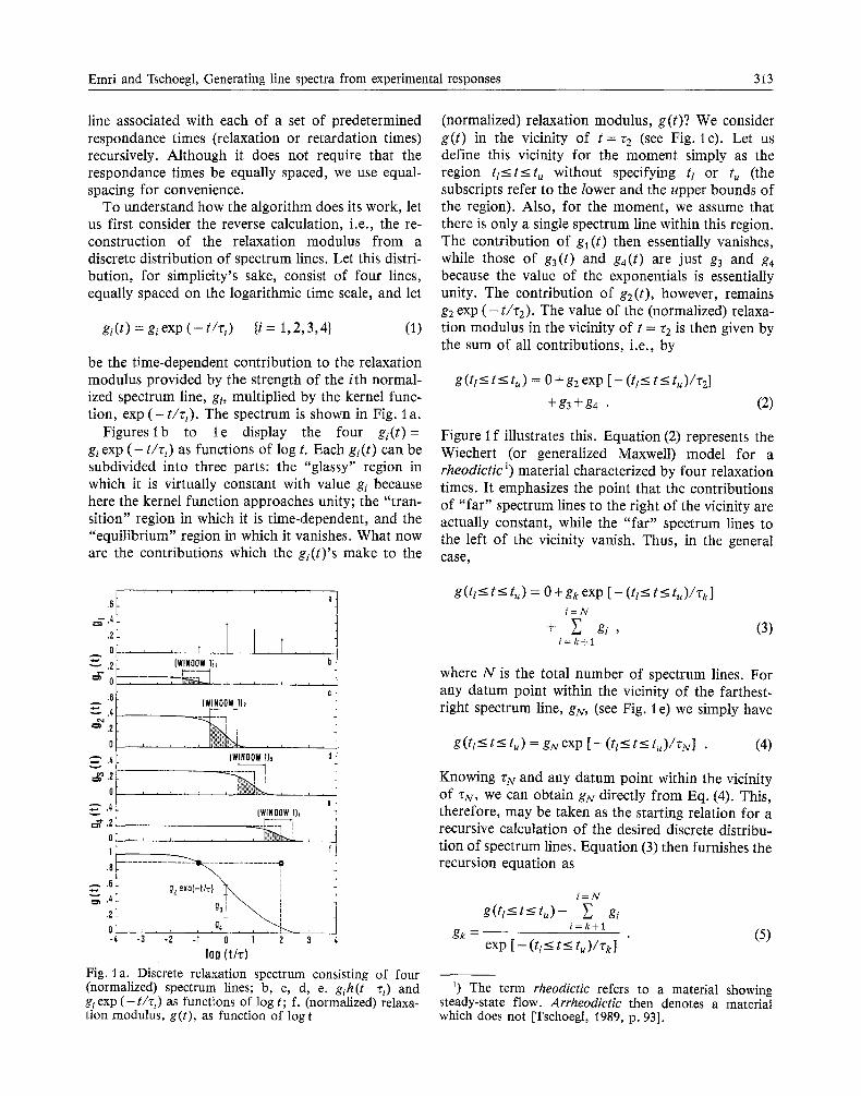
be the time-dependent contribution to the relaxation modulus provided by the strength of the ith normal- ized spectrum line, gi, multiplied by the kernel func- tion, exp ( - t / r , ) . The spectrum is shown in Fig. 1 a.

Figures lb to l e display the four gi(t) = gi exp ( - t / r , ) as functions of log t. Each gi(t) can be subdivided into three parts: the "glassy" region in which it is virtually constant with value gi because here the kernel function approaches unity; the "tran- sition" region in which it is time-dependent, and the "equilibrium" region in which it vanishes. What now are the contributions which the gi(t) 's make to the

.6

.2

O ,

~ 0 , .6

~" A I ~ . 2

0

~ '2 I 0 ,

. . . . t l l i

(WINOOW lh b i E

¢ (WlNOOW llz

(WINDOW lh

(WINDOW lh

__ 68 t i . . . . . . . . . . . . . . . 02 r ........... "~ ,4 4

. 2

-4 -3 -2 -1 0 I 2

Io0 ( f i r )

a .

3 4

Fig. l a. Discrete relaxation spectrum consisting of four (normalized) spectrum lines; b, c, d, e. gih( t -r i ) and gi exp ( - t/zt) as functions of log t; f. (normalized) relaxa- tion modulus, g(t), as function of log t

(normalized) relaxation modulus, g(t)? We consider g(t ) in the vicinity of t =r2 (see Fig. lc). Let us define this vicinity for the moment simply as the region tt<_t<_t~ without specifying tt or tu (the subscripts refer to the lower and the upper bounds of the region). Also, for the moment, we assume that there is only a single spectrum line within this region. The contribution of gl (t) then essentially vanishes, while those of g3(t) and g4(t) are just g3 and g4 because the value of the exponentials is essentially unity. The contribution of g2(t), however, remains g2 exp ( - t/r2). The value of the (normalized) relaxa- tion modulus in the vicinity of t = r2 is then given by the sum of all contributions, i.e., by

gut<_ t_< t~) = 0 + g2 exp [ - (tt_< t_< t~)/r2]

+g3 +g4 . (2)

Figure i f illustrates this. Equation (2) represents the Wiechert (or generalized Maxwell) model for a rheodictic 1) material characterized by four relaxation times. It emphasizes the point that the contributions of "far" spectrum lines to the right of the vicinity are actually constant, while the "far" spectrum lines to the left of the vicinity vanish. Thus, in the general case,

g (tl-< t_< tu) = 0 + gk exp [ - - (tt <-- t <_ t u ) / r k]

i = N

+ ~ gi , i=k+l

(3)

where N is the total number of spectrum lines. For any datum point within the vicinity of the farthest- right spectrum line, gN, (see Fig. i e) we simply have

g(tt<--t<-tu)=gNexp[--(tl<--t<--tu)/rU] . (4)

Knowing r N and any datum point within the vicinity of r N, we can obtain gu directly from Eq. (4). This, therefore, may be taken as the starting relation for a recursive calculation of the desired discrete distribu- tion of spectrum lines. Equation (3) then furnishes the recursion equation as

i = N

g(tt<-t<-tu) - ~ gi i = k + l

gk = (5) exp [ - (tt_< t < tu)/rk]

1) The term rheodictic refers to a material showing steady-state flow. Arrheodictic then denotes a material which does not [Tschoegl, 1989, p. 93].

314 Rheologica Acta, Vol. 32, No. 3 (1993)

Hence, we derive the strength of each spectrum line from a single datum point selected at a value of t restricted to tl<_t<_ t u. It remains to show why the calculation of each line must be restricted to a datum point within the "vicinity", and what, exactly, we mean by that hitherto loosely defined term.

To deal with these questions, we replace the kernel functions, exp (--t/rk), by unit step functions of time, h (rk--t) , which cut off all contributions above t = rk. The step functions may be considered to be crude approximations to the exponential functions. Figures 1 b, i c, 1 d, and 1 e show them as dashed lines next to the full lines representing the exponential functions. The step functions exhibit no "transition" regions. Hence, the (normalized) relaxation modulus becomes

k - 1

g ( t ) = ~ g i h ( r i - t ) + g k h ( r k - t ) i = 1

i = N

+ ~ gi h(T i - t ) . (6) i = k + l

In this expression, we have separated out from the total sum the k th spectrum line as that line on which we focus our attention. If now there exists a datum point at t = rk, then it follows from Eq. (6) that

i = N

gk=g(t)[t=r~ - ~ g i . (7) i = k + l

If, however, we do not find a datum point at t = rk, then there would be no way to calculate gk. Thus, if we replace the exponential functions with step func- tions it becomes clear that we should not use datum points which lie either to the left or to the right of t = r k for the evaluation of the k th spectrum line. That this is so is seen even more clearly when we ex- amine Fig. I f. If, for example, we use the datum point at t = rl, denoted by the filled circle, to calculate g4, we would erroneously obtain

g4=g(t)lt=~l , (8)

as shown by the partially filled circle and the vertical line in the figure. Modeling of the relaxation modulus then would require spectrum lines with negative values in the time domain between rl and r4 to com- pensate for the error.

The use of step functions instead of exponential kernels effectively reduces the vicinity to a single point. It can now be recognized as an advantage that the kernel function is an exponential, and not a step

function of time. As we have just shown, the discon- tinuous nature of the step function at t = T k allows the calculation of the k th spectrum line only from the single datum point on the relaxation curve which lies at t = Zk (or, at most, from one very close to it). By contrast, the exponential function replaces the sharp cut-off at t = rk by a continuous "transition" region on the logarithmic time scale, This vastly reduces the error involved in using neighboring datum points in the calculation and is important because, in any prac- tical application, the location of the "coinciding" data point is not known. The advantage is valid in the reverse case also. To model the relaxation modulus with exponential kernels instead of step functions re- quires, for the same error, a much smaller number of elements.

The salient conclusion to be drawn from these observations is that datum points should be selected only within a window covering essentially the "transi- t ion" region. This window is what we have earlier called the "vicinity". The exponential kernel function can model the relaxation modulus effectively only in the transition region where the first derivative is sig- nificantly larger than zero. Figure 2 shows that the ex- ponential kernel function well satisfies this condition in the region from about log t/rk = - 0.6 to 0.4. This region is the Boundary Window. Further below, we introduce a second window, the Modeling Window. It is this window in which the algorithm models the tran- sient response most efficiently. The span of this win- dow will be "bounded" by the first window which takes its name from this property. However, to save space in the figures, we will refer to these windows as Window 1, and Window 2, respectively.

In this region the exponential function, when plot- ted semilogarithmically, can be well modeled by a

"-'- .6 ' i"

WINOOW 1

OL -2 -1.5 -! -.5

log (t/v) 1.5

Fig. 2. Definition of Window 1 (the Boundary Window)

Emri and Tschoegl, Generating line spectra from experimental responses 315

straight line. The reason for selecting the particular limits of -0 .6 and 0.4 will become clear a little later. The window is not equally spaced around log t / r k because the exponential kernel function is not "sel f- c o n g r u e n t " (Tschoegl, 1989; p. 318), i.e., the upper and lower halves of the curve produced by plotting log g ( t ) vs log ( t / r ) cannot be brought into superposi- tion with each other by reflection and translation. In the companion paper (Tschoegl and Emri, 1993 a) we shall prove that this is actually an advantage not possessed by the self-congruent kernels of the storage and the loss functions.

Outside of Window 1 the exponential kernel behaves effectively as a step function. As discussed in connection with Eqs. (7) and (8), an attempt to calculate a spectrum line outside the "boundary win- dow" may produce a line that is either larger or smaller than it should be. The algorithm then tries to compensate by making the next line smaller or larger.

We can now distribute the complete set of datum points over several windows, each of which comprises the location of one of the preselected spectrum lines. A window of the stated width allows us to calculate spectrum lines separated by exactly one decade on the logarithmic time scale. We have also found it conve- nient when running the algorithm in double precision on a computer. To cover the entire range of datum points on the logarithmic time scale, one needs to preselect at least one spectrum line per window (i.e., per decade of time). Each window must contain at least one datum point. However, the datum points need not be spaced equally as long as each is in a separate window. If enough datum points are avail- able, the number of spectrum lines per decade may be increased. To how many lines? The rule is that the calculation should be started with the minimum num-

i.O

.8

.2

0

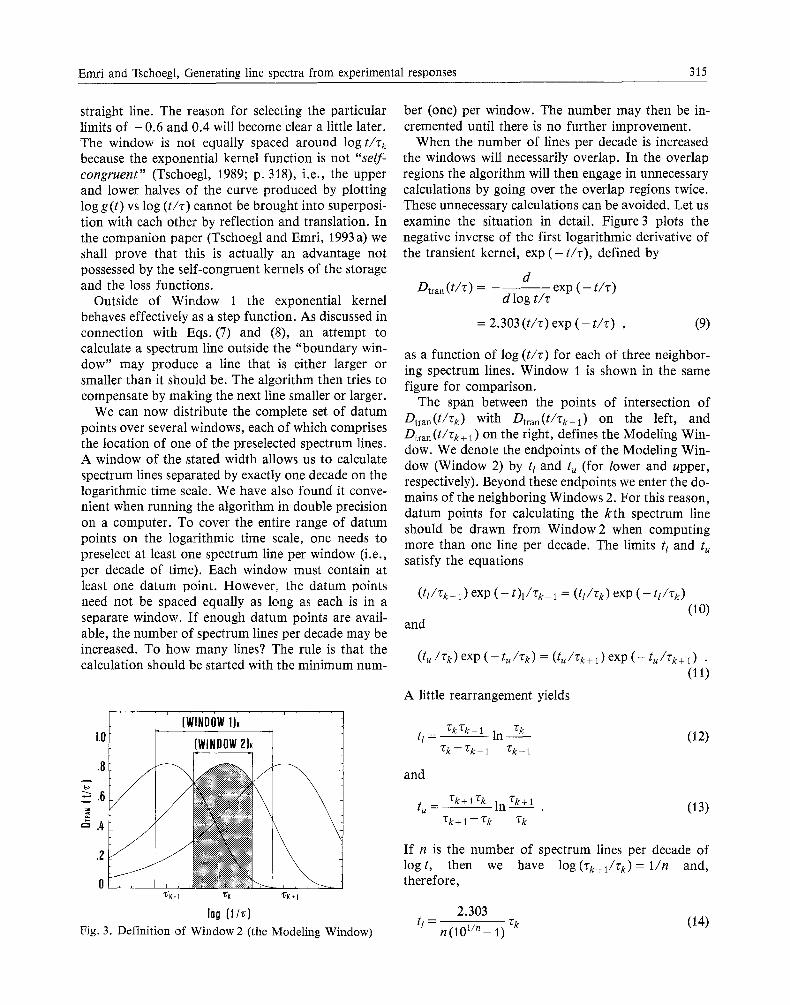
log (t/~) Fig. 3. Definition of Window 2 (the Modeling Window)

ber (one) per window. The number may then be in- cremented until there is no further improvement.

When the number of lines per decade is increased the windows will necessarily overlap. In the overlap regions the algorithm will then engage in unnecessary calculations by going over the overlap regions twice. These unnecessary calculations can be avoided. Let us examine the situation in detail. Figure 3 plots the negative inverse of the first logarithmic derivative of the transient kernel, exp ( - t / r ) , defined by

d Dtran ( t / c ) - - - exp ( - t / r )

d log t / r

= 2.303 ( t / z ) exp ( - t / z ) , (9)

as a function of log ( t / z ) for each of three neighbor- ing spectrum lines. Window 1 is shown in the same figure for comparison.

The span between the points of intersection of Dtran(t /rk) with Dtran( t / rk -1 ) on the left, and Dtran ( t / r k + l ) on the right, defines the Modeling Win- dow. We denote the endpoints of the Modeling Win- dow (Window 2) by tt and tu (for lower and upper, respectively). Beyond these endpoints we enter the do- mains of the neighboring Windows 2. For this reason, datum points for calculating the kth spectrum line should be drawn from Window 2 when computing more than one line per decade. The limits tt and t u satisfy the equations

( t t / r k - 1 ) exp ( - t ) l / r k _ 1 = (tl/rK ) exp ( - t t / r k ) (lo)

and

(6 / rk) exp ( -- tu/r~) = ( tu / rk + ~ ) exp ( -- t u / r k + i ) • (11)

A little rearrangement yields

t l - --rk'Ck--------~ ln rk (12)

rk-- Tk_ 1 rk-1

and

tu- - r k + l r k lnrk+l (13) rk+ l - rk rk

If n is the number of spectrum lines per decade of logt, then we have log(rx+l/rx) = 1 /n and, therefore,

2.303 t l - (101/, "ok (•4) n -1)

316 Rheologica Acta, Vol. 32, No. 3 (1993)

and

t u - - 2.303 x 101/n

n (101/n -- 1 ) r~. (15)

Values for n = 1 to n = 8 are tabulated below.

Table 1. Limits of Window 2

n log tt/r ~ log tu/r k n log tl/zg log t~/r k

1 -0.59 0.41 5 -0.10 0.10 2 - 0.27 0.23 6 - 0.08 0.08 3 -0.18 0.15 7 -0.07 0.07 4 -0.13 0.12 8 -0.06 0.06

The window becomes more symmetrical, and its width decreases as the number of spectrum lines in- cluded within it increases. Accordingly,

lira Window 2 = 0 (16) n ---r ~

marks the transition from the discrete to the con- tinuous form of the representation of G(t). We em- phasize that Window2 must contain at least one datum point. In practice, this puts some limitation on the width of Window2, i.e., on the number of preselected spectrum lines one may choose.

Window 1 spans the region in which the exponen- tial kernel function is at all effective in modeling the relaxation modulus. Window 2, on the other hand, demarcates the region over which this modeling is most effective. Table 1 shows that the two windows coincide for the choice of one spectrum line per decade. We have chosen the limits of Window i as - 0 . 6 and 0.4 instead of - 0 . 5 9 and 0.41 purely for convenience in later calculations. The small difference is without practical consequence.

The algorithm

The preceding theoretical discussion served to clarify which datum points should be considered in the evaluation of a particular spectrum line. We now develop the detailed algorithm for the calculation of the distribution of spectrum lines from experimental responses to excitations applied as step functions of time. We take the (shear) relaxation modulus first, and follow this with the (shear) creep compliance. The method is easily adapted to dealing with the tensile relaxation modulus and with the tensile creep com- pliance or, for the matter, with any other response to

the imposition of a strain or a stress as a step function of time such as, for example, the wave modulus or the bulk compliance (Tschoegl, 1989; p. 515 ff).

Relaxation modulus

According to the theory of linear viscoelastic behavior the shear relaxation modulus may be repre- sented (Tschoegl, 1989; p. 121) by a Wiechert (or generalized Maxwell) model as

i = N

G(t) = [Ge}+ ~ Giexp ( - t / r i ) , (17) i = 1

where "ci=rli/G i, and Gi and ~/i represent the modulus and the viscosity of the ith Maxwell unit. G e is the equilibrium modulus. The braces signify that {Ge} = G e when the modulus describes an arrheodictic material, and that (Ge} = 0 when the material is rheodictic. 1) For convenience in the computations, we normalize by the difference Gg-[Ge}, where Gg is the instantaneous (or glassy) modulus. We remark that the sum of the normalized spectra is always uni- ty. Normalization leads to

i = N

g(t)={ge}+ ~ g i e x p ( - t / z i ) , (18) i = 1

where g(t) is the normalized relaxation modulus, ge is the normalized equilibrium modulus, and the gi's represent the strengths of the delta functions in the normalized discrete relaxation spectrum (Tschoegl, 1989; p. 227)

i = N

h ( ~ - ) = ~ g i ' c i t ~ ( ' c - ' c i ) . ( 1 9 ) i = 1

We assume the source data to be available as a discrete set of M datum points {G(tj)} where j = 1,2 . . . . . M. Each of these datum points can be nor- malized by the difference between the largest point, G1, and the smallest point, GM, to yield the nor- malized set {~(tj)}. We can then express the modulus alternatively by a discrete set of (normalized) spec- trum lines, [~i}. In terms of these each datum point becomes

i = N

~(tj) = ~(tM)+ ~ ~iexp ( - t j / r i ) • (20) i = 1

1) The term rheodictic refers to a material showing steady-state flow. Arrheodictic then denotes a material which does not (Tschoegl, 1989; p. 93).

Emri and Tschoegl, Generating line spectra from experimental responses 317

We intend to determine, from the set of source data, {~(tj)}, a set of spectrum lines, {~fl, which will faithfully reproduce the modulus, G (t). As in Eq. (3), we split the sum in Eq. (20) into three parts and write

i = k - 1

g(tj) = ~(tM) + E giexp ( - tj/zi) i = l

+gk exp ( - ty/rk)

i = N

+ ~ g i e x p ( - t j / z i ) + A j • i = k + l

(21)

We have added the term Aj = A ~ + A ~ to allow us to account for the experimental error in the source data, A~, and for the approximation error, A i , which arises because the calculated line spectrum is an ap- proximation to the unknown true spectrum.

Two decades to the right of the location of any zi, e x p ( - t / r i ) has already dropped to 3.72×10 .44 which, to all intens and purposes, is zero (see Fig. 2). We can therefore safely neglect the contributions of all lines located two or more decades downscale from r k. By beginning the first summation in Eq. (21) with l<_m = k - 2 n - 1 instead of 1, we may thus reduce the time which the algorithm needs to execute each sweep. We therefore rewrite Eq. (21) as

i = k - 1

~( t j )=g( tM)+ ~, ~ i e x p ( - t j / z i ) i = m

+ ge exp ( - tj/rk)

i = N

+ ~ g i e x p ( - t j / r i ) + A j . (22) i = k + l

The sum of squares of Aj within Window 2 is given by

J =~k, u 2 E k = A j , (23)

j = Sk, l

where sk, l and Sk, u are the first and the last discrete points in the window which belong to the kth spec- trum line. Minimizing the error according to OEk/O~ k = 0, leads to

J = Sk, u

2 g k - - : j = s/c' !

~b (tj) exp ( - tj/zk)

J = s ~ u

exp ( - 2 tj/rk) J = slc, l

(24)

where i = k - 1

~(tj) = g ( t j ) - - g ( t u ) - i = m

i = N

- - 2 g i exp ( - tj/~ci) i = k + l

g i exp ( - tj/%)

(25)

is the expression from which we obtain the strength of the kth spectrum line.

We start the computation with the Nth, i.e., the farthest right, spectrum line, gN, because the first sum in Eq. (25) then vanishes (cf. Eq. (4)). In the first pass over the source data we set the ~j, (i = m . . . . . k - 1), to zero. In succeeding sweeps, we then substitute any newly found non-negative value for the corresponding previous one and set any negative value again to zero. The iteration is broken off when the difference between the previously found and the newly computed spectrum lines is smaller than a preset error. We generally set the criterion for terminating any of the required iterations as 0.0010/o of the difference between the new and the previously calculated value. Sharpening the criterion to 0.0001 °7o significantly increases the time required for the calculations, but does not result in any significant change in the values of the spectrum lines. This shows that the algorithm converges.

Creep compliance

We now turn to the creep compliance. For a Kelvin (or generalized Voigt) model this becomes (Tschoegl, 1989; p. 123)

i = N

J( t ) -{Ozt} = Jg+ ~ Ji[1 - e x p ( - t / r i ) ] i = 1

i = N

= j~o I _ ~ Ji exp ( - t/zi) , (26) i = 1

where Je is the equilibrium compliance, Je 0 is the steady-state compliance, Jg is the glassy compliance, and q~f is the steady-flow fluidity, reciprocal of the steady-flow viscosity, ~/f. The symbols in braces are absent when the material is arrheodictic, and present if it is rheodictic. Comparison with Eq. (17) shows that the kernel function in the second of the two equa- tions is identical with that of the relaxation modulus. We therefore simply apply the algorithm to the creep compliance in this form. Normalizing by the dif- ference, JM-J1 , we obtain equations which are for- mally identical with Eqs. (18) through (24). The algorithm to be used for the creep compliance is thus

318 Rheologica Acta, Vol. 32, No. 3 (1993)

mathematically identical with that used for the relaxa- tion modulus.

R e s u l t s

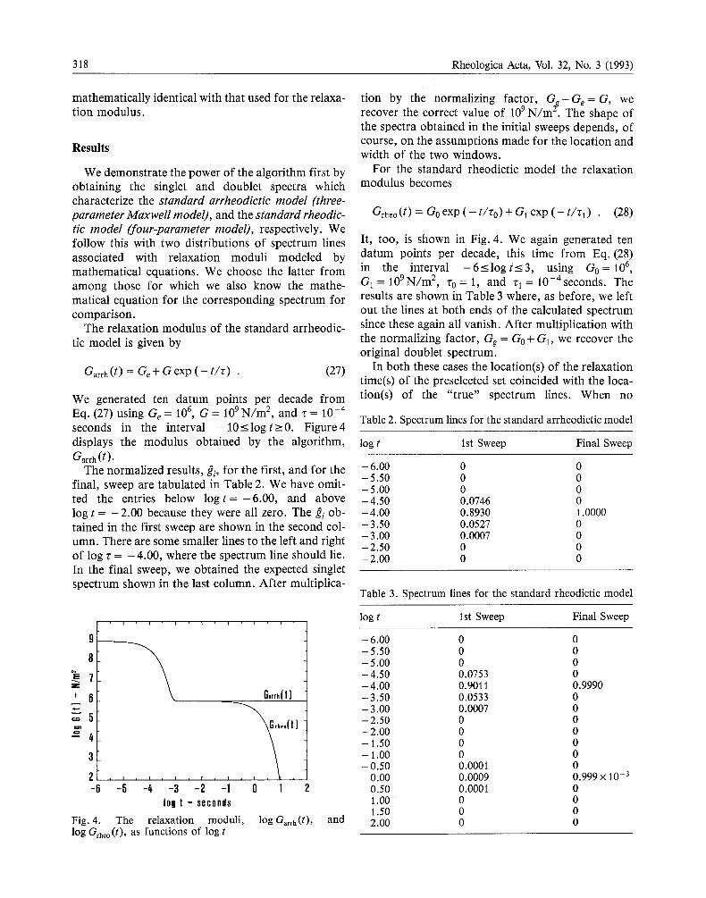
We demonstrate the power of the algorithm first by obtaining the singlet and doublet spectra which characterize the standard arrheodictic model (three- parameter Maxwel l modeO, and the standard rheodic- tic model (four-parameter model), respectively. We follow this with two distributions of spectrum lines associated with relaxation moduli modeled by mathematical equations. We choose the latter f rom among those for which we also know the mathe- matical equation for the corresponding spectrum for comparison.

The relaxation modulus of the standard arrheodic- tic model is given by

Garrh(t ) = G e + G exp ( - t / r ) . (27)

We generated ten datum points per decade f rom Eq. (27) using Ge = 106, G = 109 N / m 2, and ~ = 10 -4 seconds in the interval -10_<logt_>0. Figure4 displays the modulus obtained by the algorithm,

Garrh(t). The normalized results, gi, for the first, and for the - 6.00

- 5 . 5 0 final, sweep are tabulated in Table 2. We have omit- -5.00 ted the entries below l o g t = - 6 . 0 0 , and above -4.50 l o g t = - 2 . 0 0 because they were all zero. The gi ob- -4.00 tained in the first sweep are shown in the second col- -3.50 umn. There are some smaller lines to the left and right - 3.00

-2.50 of log r = - 4 . 0 0 , where the spectrum line should lie. -2 .00 In the final sweep, we obtained the expected singlet spectrum shown in the last column. After multiplica-

i i i

8

7 Z

' 6 G,rra(l)

5 ,oltl __w~ 3

I i I , II i

log I - seconds

Fig. 4. The relaxation moduli, log Garrh(t), log Grheo(t), as functions of log t

and

tion by the normalizing factor, G o - G e = G, we recover the correct value of 109 N / m ~. The shape of the spectra obtained in the initial sweeps depends, of course, on the assumptions made for the location and width of the two windows.

For the standard rheodictic model the relaxation modulus becomes

Grheo (t) = Go exp ( - t/ro) + G1 exp ( - t/'c 1) . (28)

It, too, is shown in Fig. 4. We again generated ten datum points per decade, this time f rom Eq. (28) in the interval -6_<logt_<3, using G o = 106 , G1 = 109N/m 2, "Co = 1, and "q = 10-4seconds. The results are shown in Table 3 where, as before, we left out the lines at both ends of the calculated spectrum since these again all vanish. After multiplication with the normalizing factor, Gg = Go + GI, we recover the original doublet spectrum.

In both these cases the location(s) of the relaxation time(s) of the preselected set coincided with the loca- tion(s) of the "true" spectrum lines. When no

Table 2. Spectrum lines for the standard arrheodictic model

log t 1st Sweep Final Sweep

0 0 0 0 0 0 0.0746 0 0.8930 1.0000 0.0527 0 0.0007 0 0 0 0 0

Table 3. Spectrum lines for the standard rheodictic model

log t 1st Sweep Final Sweep

- 6.00 0 0 -5.50 0 0 - 5 . 0 0 0 0 - 4.50 0.0753 0 - 4.00 0.9011 0.9990 - 3.50 0.0533 0 - 3.00 0.0007 0 - 2 . 5 0 0 0 - 2.00 0 0 - 1 . 5 0 0 0 - 1 . 00 0 0 - 0.50 0.0001 0

0.00 0.0009 0.999 × 10 -3

0.50 0.0001 0 1 .00 " 0 0 1 .50 0 0 2.00 0 0

Emri and Tschoegl, Generating line spectra from experimental responses 319

preselected line coincides with an original spectrum line, the algorithm must generate a composite line spectrum to simulate the effect of the original line as best it can. The composite spectrum will consist of two or more lines. This results in a corresponding broadening of the relaxation modulus reconstructed according to Eq. (28) from the calculated distribu- tion. It may be possible to improve the distribution by increasing the number of preselected relaxation times per logarithmic decade. The closer one of these comes to the original relaxation time, the better will be the calculated distribution. When coincidence occurs, then we recover the relaxation modulus exactly.

To show this, we calculated the spectrum lines ob- tained from the standard arrheodictic model (see Eq. (23)) with log ~ = - 4 . 2 , and the same moduli as before. We preselected the relaxation times to lie at log r . . . . - 5 , - 4 , - 3 . . . . . In each succeeding run we increased the number of lines within each logarithmic decade from 1 to a total of 5.

The results are tabulated in Table 4. With 1 to 4 line(s)/decade the algorithm generates doublet spectra instead of the correct singlet spectrum. The two non- zero lines progressively approach one another. The lines below l o g r = - 4 . 0 0 increase at the expense of the line at log r = - 4 . 0 0 until, with 5 lines/de- cade, the expected singlet spectrum emerges at log r = - 4.20. If the "original" line had been located at log r = -4 .23 , say, we would still not have obtain- ed the "true" spectrum.

The case of an "original" singlet spectrum is, of course, highly unrealistic. In the general case, the ob- served relaxation modulus must be described with a distribution of reasonably closely spaced spectrum lines which will have no connection with any "original", or "true" lines. We cannot even know if such lines indeed exist. The question then arises: how many lines per decade should the algorithm employ to

Table 4. Effect of increasing the number of spectrum lines per decade. Standard arrheodictic model

log r 1/dec 2/dec 3/dec 4/dec 5/dec

- 5.00 0.3350 0 0 0 0 - 4.80 . . . . o - 4.75 - - - 0 - - 4.67 - - 0 - - 4.60 . . . . 0 -4.50 - 0.5259 - 0 - 4.40 . . . . 0 -4.33 - - 0.6831 - -4.25 - - - 0.8393 - 4.20 . . . . 1.0000 -4.00 0.6650 0 .4741 0.3169 0.1607

make possible the recovery of the original relaxation modulus with an acceptable error? This error is simp- ly the relative error derived from a comparison of the original modulus data with those reconstructed from the calculated distribution. The practical expedient is to run the algorithm with an increasing number of lines per decades until the desired relative error is at- tained. It must be borne in mind, however, that an in- crease in the number of spectrum lines per decade re- quires an increase in the number of datum points. If no more datum points are available, Window2 should be widened without, however, exceeding the width of Window 1.

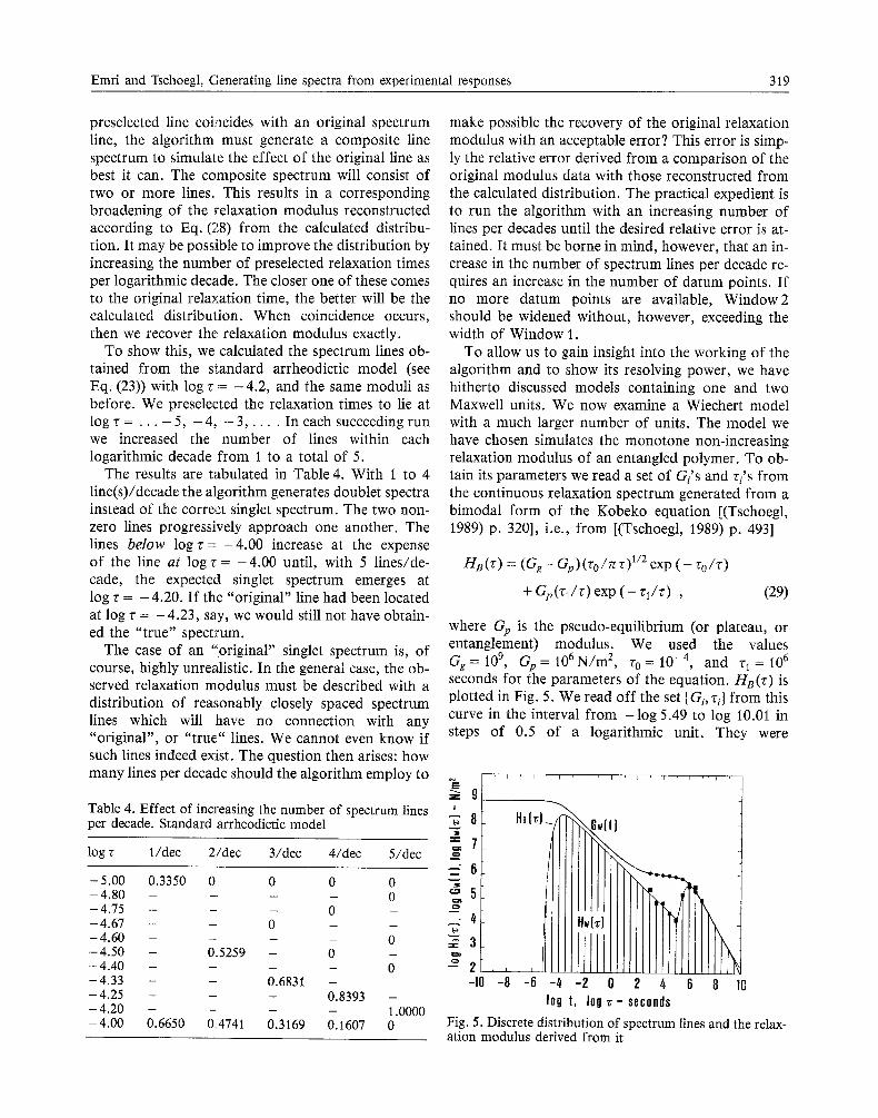
To allow us to gain insight into the working of the algorithm and to show its resolving power, we have hitherto discussed models containing one and two Maxwell units. We now examine a Wiechert model with a much larger number of units. The model we have chosen simulates the monotone non-increasing relaxation modulus of an entangled polymer. To ob- tain its parameters we read a set of Gi's and ri's from the continuous relaxation spectrum generated from a bimodal form of the Kobeko equation [(Tschoegl, 1989) p. 320], i.e., from [(Tschoegl, 1989) p. 493]

HB(r) = (Gg - Gp)('Co/7~72) 1/2 exp ( - r0 / r )

+ Gp(r l / r ) exp ( - r l / r ) , (29)

where Gp is the pseudo-equilibrium (or plateau, or entanglement) modulus. We used the values Gg = 109, Gp = 106 N / m 2, r0 = 10 -4, and r~ = 106 seconds for the parameters of the equation. H s ( r ) is plotted in Fig. 5. We read off the set [Gi, ril from this curve in the interval from - l o g 5.49 to log 10.01 in steps of 0.5 of a logarithmic unit. They were

9 I

z=o

o _2,,

H~ (~) 1 ' -8 ' -6 -4 -2 0 2 4

log t, Iog z:- seconds 1 0

Fig. 5. Discrete distribution of spectrum lines and the relax- ation modulus derived from it

320 Rheologica Acta, Vol. 32, No. 3 (1993)

deliberately displaced by 0.01 logarithmic units from the location of the spectrum lines preselected for the algorithm. Equation (29) thus simply served as an "in- spiration". The procedure yielded the discrete spec- trum

Hw(Z ) = ~ Gi~:,~(z- ri) (30) i

for the Wiechert model. The spectrum is shown in Fig. 5 together with the relaxation modulus

Gw(t) = ~ Gi exp ( - t/zi) (31) i

derived from it. We engaged the algorithm a second time to deter-

mine a second set of parameters {Gj, z]}, also in steps of 0.5 logarithmic units, but in the interval - log 5 .5 0 to log 10.0. Despite the deliberate displacement in- troduced betwen the two sets, the moduli generated from them are virtually identical. They overlap to such an extent that they cannot be resolved on the scale of the plot. In this exercise, we have generated two slightly different discrete distributions of relaxa- tion times which, however, represented the same underlying unknown distribution. Although the data sets differed from one another, they generated moduii which were virtually indistinguishable from each other. This strongly supports the contention that the algorithm is capable of producing a discrete set of spectrum lines from which the experimental response can be recovered faithfully.

It is another remarkable feature of the algorithm that it will calculate nearly correct spectrum lines even from only a portion of the input data. To show this, we obtained the spectrum lines from the segment of Gw(t) lying between log t = 3 and 7. This portion constitutes an especially severe test. The filled rec- tangles in Fig. 5 mark the heights of the spectrum lines obtained from this portion. The deviations at both ends are due to truncation errors, i.e., the absence of information outside of the selected por- tion. The slight differences in the magnitudes of the lines of the full and of the partial sets can be traced to the change in slope of the envelope. In the region between log t = - 3 and 1, for example, where the envelope is a straight line, the agreement between the full and the partial set is virtually complete. The filled circles represent the modulus calculated from this spectrum. Despite the deviations between the two spectra, the filled circles still overlap Gw(t).

Truncation errors do, of course, always occur because we never have experimental information ex-

tending from t = 0 to t = ~ . The magnitude of the deviations caused by this unavoidable truncation of the available information depends primarily on how close GI is to Gg, or G M is to G e (which, of course, may be 0).

Discussion

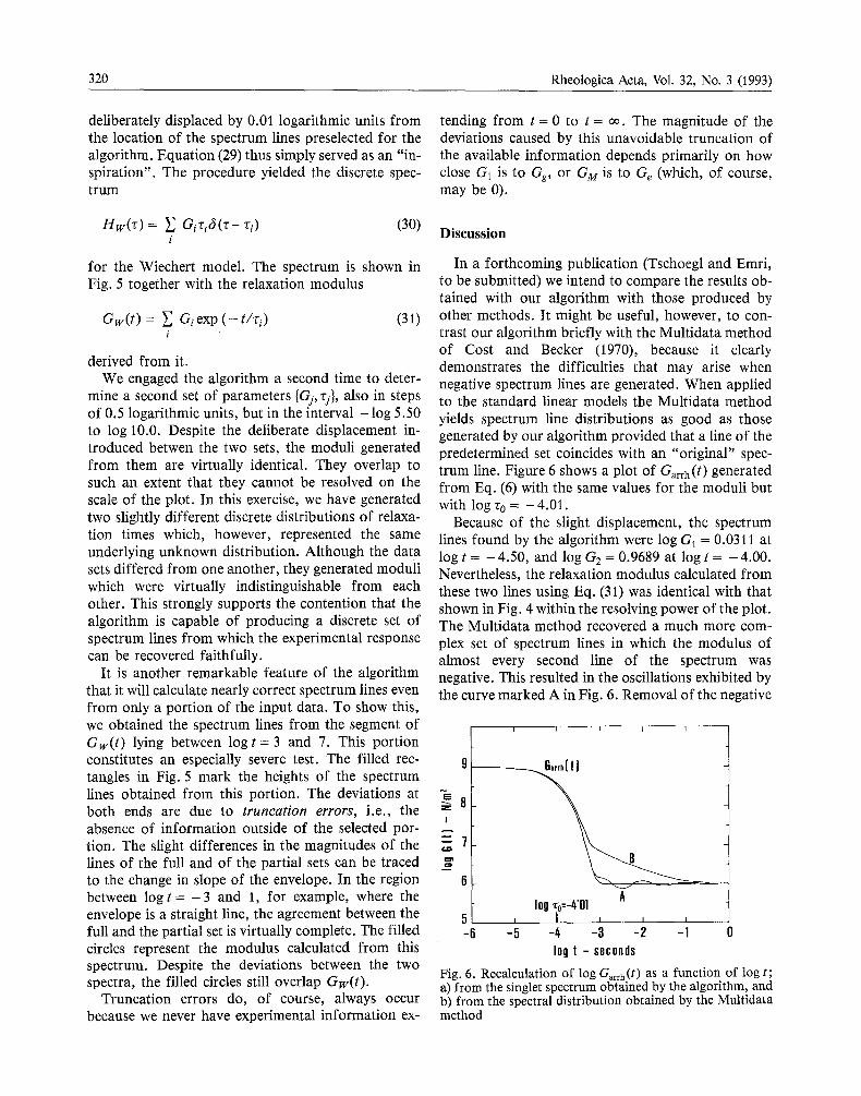
In a forthcoming publication (Tschoegl and Emri, to be submitted) we intend to compare the results ob- tained with our algorithm with those produced by other methods. It might be useful, however, to con- trast our algorithm briefly with the Multidata method of Cost and Becker (1970), because it clearly demonstrates the difficulties that may arise when negative spectrum lines are generated. When applied to the standard linear models the Multidata method yields spectrum line distributions as good as those generated by our algorithm provided that a line of the predetermined set coincides with an "original" spec- trum line. Figure 6 shows a plot of Garrh(t ) generated from Eq. (6) with the same values for the moduli but with log r 0 = - 4.01.

Because of the slight displacement, the spectrum lines found by the algorithm were log G 1 = 0.0311 at log t = - 4.50, and log G2 = 0.9689 at log t = - 4.00. Nevertheless, the relaxation modulus calculated from these two lines using Eq. (31) was identical with that shown in Fig. 4 within the resolving power of the plot. The Multidata method recovered a much more com- plex set of spectrum lines in which the modulus of almost every second line of the spectrum was negative. This resulted in the oscillations exhibited by the curve marked A in Fig. 6. Removal of the negative

I L I I I

N 8 !

"-7

6 / 10g ~,0=-4"01 A t

5 i / i i a J

- -5 -4 -3 -2 -1 0 10g t - seconds

Fig. 6. Recalculation of log Garrh(t) as a function of log t; a) from the singlet spectrum obtained by the algorithm, and b) from the spectral distribution obtained by the Multidata method

Emri and Tschoegl, Generating line spectra from experimental responses 321

lines f rom the spectrum produced curve B. The Multidata method will produce oscillations in the modulus when, at a given point along the time scale, the contribution of negative spectrum lines outweighs the contribution of the positive lines. Since the con- tribution by the largest lines in the transition region has effectively died out two decades upscale, these oscillations are most likely to occur in the equilibrium region of an arrheodictic material.

When we applied the Multidata method to Gw(t), as given by Eq. (31), the spectrum was virtually iden- tical with ours, except in the glassy region were both positive and negative lines showed up where there were no lines in the input spectrum, Hw( r ) , and where our algorithm produced none. This, it should be noted, has no noticeable effect on the recon- structed modulus because the contribution by positive lines in this region compensates the contribution which the negative lines make. In addition, the sum,

i Gi , is large enough in the glassy region to insure that the positive contributions outweigh any remain- ing negative ones. On the right end of the spectrum we now encountered no negative spectrum lines because we were describing a rheodictic material with a mono- tone non-increasing modulus. The spectrum produced by the Multidata method could conceivably be im- proved in a given case by a trial-and-error shifting of the time scale. This, however, is evidently unsatisfac- tory as a routine procedure.

We conclude that in applying the Multidata method one may routinely encounter unwanted lines, some of which will necessarily by negative. Even when this has no noticeable effect on the reconstructed modulus or compliance, it must be expected to vitiate any effort to convert Gi's into Ji's and vice versa.

Acknowledgements

The authors gratefully acknowledge support of this work by the Slovene Ministry of Science under Grant P2-1131-782/91, and partial support by the California Institute of Technology.

References

Baumgaertel M, Winter HH (1989) Determination of discrete relaxation and retardation spectra from dynamic mechanical data. Rheol Acta 28:510-520

Cost TL, Becker EB (1970) A multidata method of approx- imate Laplace transform inversion. Intern J Num Methods in Engg 2:207

Elster C, Honercamp J (1991) Modified maximum entropy

method and its application to creep data. Macromolecules 24:310- 314

Elster C, Honercamp J (1992) The role of the error model in the determination of the relaxation time spectrum. J Rheol 36:911 - 927

Elster C, Honercamp J, Weese J (1991) Using regularization methods for the determination of relaxation and retarda- tion spectra of polymeric liquids. Rheol Acta 32:262 - 174

Emri I, Tschoegl NW (1993 b) Generating line spectra from experimental responses. IV. Application to experimental data. To be submitted to Rheol Acta

Honercamp J (1989) Ill-posed problems in rheology. Rheol Acta 28:363 - 371

Honercamp J, Weese J (1989) Determination of the relaxa- tion spectrum by a regularization method. Macro- molecules 22:4372-4377

Janzen J, Scanlan J (1994) Practical implementation of dif- ferential operator methods for determining continuous distributions of relaxation times from linear viscoelastic data. Submitted to Rheol Acta

Kamath VM, Mackley MR (1989) The determination of polymer relaxation moduli and memory functions using integral transforms. J Non-Newt Fluid Mech 32:1199

Laun HM (1986) Prediction of elastic strains of polymer melts in shear and elongation. J Rheol 30:459

Orbey N, Dealy JM (1991) Determination of the relaxation spectrum from oscillatory shear data. J Rheol 35: 1035 - 1049

Schapery RA (1962) Approximation methods of transform inversion for viscoelastic stress analysis. Proc Fourth US Nat Congr Appl Mech 2:1075

Tobolsky AV, Murakami K (1959) Existence of a sharply defined maximum relaxation time for monodisperse polystyrene. J Polymer Sci 40:443

Tschoegl NW (1989) The phenomenological theory of linear viscoelastic behavior. Springer, Berlin

Tschoegl NW, Emri I (1992) Generating line spectra from experimental responses. III. Interconversion between relaxation and retardation behaviour. Intern J Polym Mater 18:117- 127

Tschoegl NW, Emri I (1993 a) Generating line spectra from experimental responses. II. Storage and loss functions. Rheol Acta 32:322-327

Tschoegl NW, Emri I (1994) Comparison of various algorithms for generating spectral functions from ex- perimental responses. To be submitted to Rheol Acta

(Received August 24, 1992; accepted April 1, 1993)

Correspondence to:

Prof. Igor Emri Mechanical Engineering Department University of Ljubljana Murnikova 2 61000 Ljubljana, Slovenia

Prof. N.W. Tschoegl California Institute of Technology 1201 East California Boulevard Pasadena, CA 91125, USA