PHYSICAL REVIEW B 90, 115203 (2014)

Spin relaxation in materials lacking coherent charge transport

N. J. Harmon* and M. E. FlatteDepartment of Physics and Astronomy and Optical Science and Technology Center, University of Iowa, Iowa City, Iowa 52242, USA

(Received 8 May 2014; revised manuscript received 20 June 2014; published 4 September 2014)

We describe a broadly applicable theory of spin relaxation in materials with incoherent charge transport;examples include amorphous inorganic semiconductors, organic semiconductors, quantum dot arrays, and systemsdisplaying trap-controlled transport or transport within an impurity band. The theory can incorporate manydifferent relaxation mechanisms, so long as electron-electron correlations can be neglected. We focus primarilyon spin relaxation caused by spin-orbit effects, which manifest through inhomogeneities in the g factor andnon-spin-conserving carrier hops, scattering, trapping, or detrapping. Analytic and numerical results from thetheory are compared in various regimes with Monte Carlo simulations. Our results should assist in evaluating thesuitability of various disordered materials for spintronic devices.

DOI: 10.1103/PhysRevB.90.115203 PACS number(s): 75.40.Gb, 72.25.Dc, 73.61.Jc, 76.30.−v

I. INTRODUCTION

Spin relaxation associated with the band transport of elec-trons in nonmagnetic materials exhibits a variety of regimesand mechanisms, depending on lattice symmetries, the ratio ofmomentum scattering and spin-orbit-interaction times, and thepresence of nuclear spin interactions [1–5]. When the electronsare localized, they relax via different mechanisms, such asspin-spin interactions [6,7]. Considerably less attention hasbeen directed towards spin relaxation in systems where chargetransport occurs through incoherent motion. These largelyfocused on organic (noncrystalline) semiconductors [8–15],due to their small spin-orbit interaction, affordability, andlarge room-temperature spin-dependent effects [16]. Spintransport in disordered crystalline semiconductors has beenused as a diagnostic tool for very small numbers of defects insemiconductor junctions using electrically detected magneticresonance [17], but has not drawn the same attention tofundamental mechanisms in macroscopic materials as theseother systems. Aspects of the spin transport problem whenthe charge transport is incoherent also have been studied insystems demonstrating impurity band transport [18,19], arraysof quantum dots [20,21], and amorphous inorganic semicon-ductors [22–24]. A fuller understanding of spin relaxation indisordered semiconductors would help clarify the behaviorof spintronic devices based on these materials, such as spinvalves [9,11,25–27]. The influence of spin relaxation on lightemitting diodes and solar cells has recently become a focus ofconsiderable interest due to results showing changes in (some-times improving substantially) device performance when spinrelaxation is increased in the materials [28–30]. Althoughthe investigation of spin relaxation in amorphous inorganicsemiconductors has received considerably less attention thanthat of organic semiconductors, similar effects can be expectedin such materials.

In this paper, we generalize our previous work [15] withorganic semiconductors to describe spin relaxation in a broaderrange of regimes of incoherent charge transport, focusingon amorphous semiconductors such as silicon (a-Si) andgermanium (a-Ge) to showcase our results. This is done by

*nicholas-harmon@uiowa.edu

explicit calculations of spin lifetimes and coherence timesusing continuous-time random walk (CTRW) theory [31,32]as well as with Monte Carlo simulations. Our theory allowsus to make precise predictions. Amorphous semiconductorsare attractive theoretically since they exhibit “dispersivetransport,” which possesses features explainable by disorderedtransport theories [33–35]. Analysis of transport is murkierfor organic semiconductors due to their supposed Gaussiandensity of states [36].

In the theory presented herein, the pivotal transport char-acteristic is the wait-time distribution (WTD). This quantity,elemental to CTRW theory, describes the probability densityfunction for wait times between transport-related events [37].Most often these events are hops between localizing centersbut could also signify trapping and trap-release times. TheWTD very much depends on the system and regime underconsideration; because the wait times typically depend on theenergy depth of a charge’s inhabitance, the energy densityof states plays an important role in determining the WTD.Determinations of the density of states and the WTD are vitalquantities to be ascertained for the various disordered systems.

Incoherent charge transport is treated as a random walkbetween the various states present in the system. As a carrierrandomly walks, we keep track of its classical spin vectorgiven some set of spin interactions, which we model as localmagnetic fields. Some of these fields are exerted on the spinin between steps; such fields result in a spin rotation givenby Rs (s for stationary). The spin may be influenced by otherlocal fields during the stepping process; they rotate by Rh (hfor hop). We assume the strong collision approximation[38]for the spin random walk, which entails that the local fieldschange instantaneously and are completely uncorrelated fromstep to step. Wait times at any position or instant are alsouncorrelated from one another. We consider correlated steps inour simulations. Figure 1 captures the evolution of a spin whileit randomly walks. The beauty of the CTRW theory is that aspin ensemble’s various random rotations that are incurredfrom its random walk can be summed exactly to determine thespin polarization.

The output of our calculations are spin-polarization func-tions of time; depending on the system at hand, we cansometimes analytically determine the longitudinal (transverse)spin relaxation (decoherence) time, which we denote as T1

1098-0121/2014/90(11)/115203(11) 115203-1 ©2014 American Physical Society

N. J. HARMON AND M. E. FLATTE PHYSICAL REVIEW B 90, 115203 (2014)

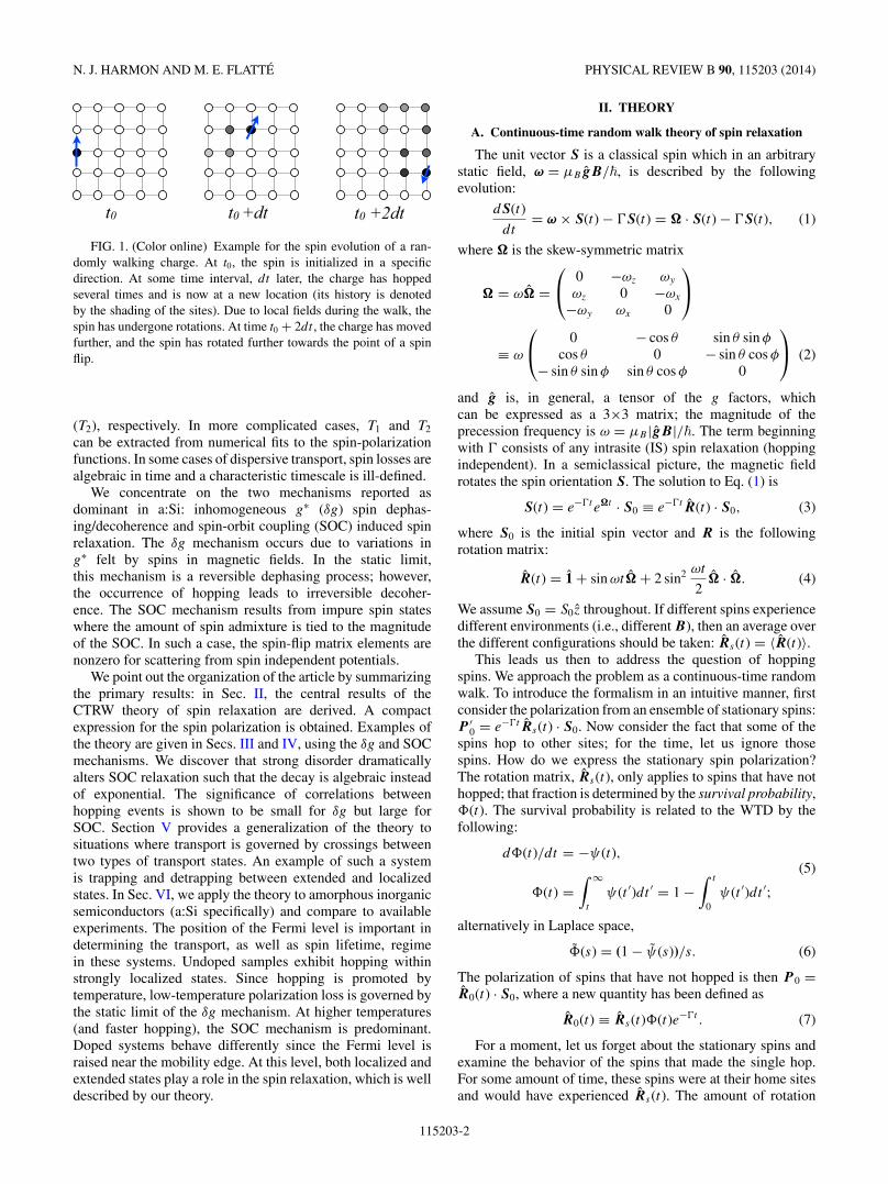
t0 t0 +dt t0 +2dt

FIG. 1. (Color online) Example for the spin evolution of a ran-domly walking charge. At t0, the spin is initialized in a specificdirection. At some time interval, dt later, the charge has hoppedseveral times and is now at a new location (its history is denotedby the shading of the sites). Due to local fields during the walk, thespin has undergone rotations. At time t0 + 2dt , the charge has movedfurther, and the spin has rotated further towards the point of a spinflip.

(T2), respectively. In more complicated cases, T1 and T2

can be extracted from numerical fits to the spin-polarizationfunctions. In some cases of dispersive transport, spin losses arealgebraic in time and a characteristic timescale is ill-defined.

We concentrate on the two mechanisms reported asdominant in a:Si: inhomogeneous g∗ (δg) spin dephas-ing/decoherence and spin-orbit coupling (SOC) induced spinrelaxation. The δg mechanism occurs due to variations ing∗ felt by spins in magnetic fields. In the static limit,this mechanism is a reversible dephasing process; however,the occurrence of hopping leads to irreversible decoher-ence. The SOC mechanism results from impure spin stateswhere the amount of spin admixture is tied to the magnitudeof the SOC. In such a case, the spin-flip matrix elements arenonzero for scattering from spin independent potentials.

We point out the organization of the article by summarizingthe primary results: in Sec. II, the central results of theCTRW theory of spin relaxation are derived. A compactexpression for the spin polarization is obtained. Examples ofthe theory are given in Secs. III and IV, using the δg and SOCmechanisms. We discover that strong disorder dramaticallyalters SOC relaxation such that the decay is algebraic insteadof exponential. The significance of correlations betweenhopping events is shown to be small for δg but large forSOC. Section V provides a generalization of the theory tosituations where transport is governed by crossings betweentwo types of transport states. An example of such a systemis trapping and detrapping between extended and localizedstates. In Sec. VI, we apply the theory to amorphous inorganicsemiconductors (a:Si specifically) and compare to availableexperiments. The position of the Fermi level is important indetermining the transport, as well as spin lifetime, regimein these systems. Undoped samples exhibit hopping withinstrongly localized states. Since hopping is promoted bytemperature, low-temperature polarization loss is governed bythe static limit of the δg mechanism. At higher temperatures(and faster hopping), the SOC mechanism is predominant.Doped systems behave differently since the Fermi level israised near the mobility edge. At this level, both localized andextended states play a role in the spin relaxation, which is welldescribed by our theory.

II. THEORY

A. Continuous-time random walk theory of spin relaxation

The unit vector S is a classical spin which in an arbitrarystatic field, ω = μB g B/�, is described by the followingevolution:

dS(t)

dt= ω × S(t) − �S(t) = � · S(t) − �S(t), (1)

where � is the skew-symmetric matrix

� = ω� =⎛⎝ 0 −ωz ωy

ωz 0 −ωx

−ωy ωx 0

⎞⎠

≡ ω

⎛⎝ 0 − cos θ sin θ sin φ

cos θ 0 − sin θ cos φ

− sin θ sin φ sin θ cos φ 0

⎞⎠ (2)

and g is, in general, a tensor of the g factors, whichcan be expressed as a 3×3 matrix; the magnitude of theprecession frequency is ω = μB | g B|/�. The term beginningwith � consists of any intrasite (IS) spin relaxation (hoppingindependent). In a semiclassical picture, the magnetic fieldrotates the spin orientation S. The solution to Eq. (1) is

S(t) = e−�te�t · S0 ≡ e−�t R(t) · S0, (3)

where S0 is the initial spin vector and R is the followingrotation matrix:

R(t) = 1 + sin ωt� + 2 sin2 ωt

2� · �. (4)

We assume S0 = S0z throughout. If different spins experiencedifferent environments (i.e., different B), then an average overthe different configurations should be taken: Rs(t) = 〈R(t)〉.

This leads us then to address the question of hoppingspins. We approach the problem as a continuous-time randomwalk. To introduce the formalism in an intuitive manner, firstconsider the polarization from an ensemble of stationary spins:P ′

0 = e−�t Rs(t) · S0. Now consider the fact that some of thespins hop to other sites; for the time, let us ignore thosespins. How do we express the stationary spin polarization?The rotation matrix, Rs(t), only applies to spins that have nothopped; that fraction is determined by the survival probability,�(t). The survival probability is related to the WTD by thefollowing:

d�(t)/dt = −ψ(t),(5)

�(t) =∫ ∞

t

ψ(t ′)dt ′ = 1 −∫ t

0ψ(t ′)dt ′;

alternatively in Laplace space,

�(s) = (1 − ψ(s))/s. (6)

The polarization of spins that have not hopped is then P0 =R0(t) · S0, where a new quantity has been defined as

R0(t) ≡ Rs(t)�(t)e−�t . (7)

For a moment, let us forget about the stationary spins andexamine the behavior of the spins that made the single hop.For some amount of time, these spins were at their home sitesand would have experienced Rs(t). The amount of rotation

115203-2

SPIN RELAXATION IN MATERIALS LACKING COHERENT . . . PHYSICAL REVIEW B 90, 115203 (2014)

depends on the wait time at the home site; the wait time isdrawn from the WTD. The amount of rotation in a short timeinterval dt ′ is Rs(t ′)ψ(t ′)dt ′. At their new site, the spins beginto evolve again with the averaged rotation matrix Rs(t). If thehop occurred at t ′ and they precess up to time t , this rotationmatrix is described by R0(t − t ′). Now we integrate over allpossible hopping times to obtain

∫ t

0 R0(t − t ′)R′0(t)dt ′, where

we have defined a new quantity:

R′0(t) ≡ Rs(t)ψ(t)e−�t , (8)

which obviously commutes with R0(t).Lastly, we need to include any rotations that might accrue

during the hop as opposed to before and after the hop. Thismatrix, Rh, is treated as time independent and any necessaryconfigurational averaging is assumed. The total rotation matrixfor spins that have hopped once is then

R1(t) =∫ t

0R0(t − t ′)Rh R

′0(t ′)dt ′, (9)

which has the form of a convolution. Assuming that Rh

commutes with the other matrices (most realistically by sayingthat Rh ∝ I), allows Eq. (9) to be expressed as

R1(t) = Rh

∫ t

0R0(t − t ′)R

′0(t ′)dt ′. (10)

The convolution theorem yields

˜R1(s) = Rh˜R0(s + �) ˜R′

0(s + �). (11)

The same reasoning is used to find the rotation matrix for spinsthat have hopped twice:

˜R2(s) = R2h

˜R0(s + �) ˜R′20 (s + �) = Rh

˜R1(s) ˜R′0(s). (12)

The procedure can be continued indefinitely for arbitrary l

hops and the following recursive expression is obtained:

˜Rl(s) = Rl

h˜R0(s + �) ˜R′l

0 (s + �) = Rh˜Rl−1(s) ˜R′

0(s + �).

(13)

The polarization results from summing this geometric series:

P(s) =∞∑l=0

˜Rl(s) · S0

= ˜R0(s + �)[I − Rh˜R′

0(s + �)]−1 · S0. (14)

It may sometimes also be useful [e.g., if Laplace transform ofR

′0(t) has no analytic expression] to write the polarization as

an integral equation in the time domain:

P(t) = R0(t) + Rh

∫ t

0P(t − t ′)R

′0(t ′)dt ′, (15)

which is a Volterra equation of the second kind or a renewalequation.

For the sake of pedagogy, we have not yet emphasized theassumptions that lead to our main result, Eq. (14). We nowmake them clear as they are a subject for discussion in latersections of this article when our results are presented. We haveused a class of assumptions known as the strong collisionapproximation [38]. The approximation has the following

characteristics: (1) local field changes are abrupt and notslow at each hop and (2) local fields at or during each hopare uncorrelated from any previous hop. In the language ofstochastic process theory, the evolution is Markovian (2) butnot Gaussian-Markovian (1).

A simple example of the theory is demonstrated by usingan exponential WTD, ψ(t) = ke−kt , where k is the averagehopping rate. Immediately, we can write from Eq. (14)

P(s) = ˜Rs(s + � + k)[I − k Rh˜Rs(s + � + k)]−1 · S0.

(16)

In later sections, we show explicit examples of when P(s) canbe inverted.

B. Multiple trapping model

More realistic WTDs are much harder to handle. In thispaper, we concentrate on the aforementioned exponentialWTD and on the WTD produced by an exponential den-sity of states (which is the appropriate one for amorphoussemiconductor band tails). The multiple trapping model (MT)constructs a WTD from hopping rates that are of the formof trap release rates, k(ε) = k0e

ε/kBT , where ε is the trapenergy and is distributed exponentially. The energy levels areuncorrelated between hops. The WTD, ψ(t), is described by∫ 0−∞ g(ε)k(ε)e−k(ε)t dε or in Laplace space as

ψ(s) =∫ 0

−∞dεg(ε)

k(ε)

s + k(ε)=

∫ 0

−∞dxex k0e

x/α

s + k0ex/α, (17)

with x = ε/kBT0 and α = T/T0 when using an exponentialdensity of states. The result can be written as a hypergeometricfunction:

ψ(s) = k0α

s + αs 2F1(1,1 + α,2 + α,−k0/s). (18)

The long time, or asymptotic, behavior of the WTD is ofinterest. It is more straightforward to derive it for the survivalprobability first,

�(s) =∫ 0

−∞dx

ex

s + k0ex/α= −

∫ 0

∞

dx

s

e−x

1 + (k0/s)e−x/α.

(19)

After making a change of variable, w = e−x(s/k0)−α , weobtain

�(s) =∫ (s/k0)−α

0

dw

s

(s

k0

)α 1

1 + w1/α. (20)

Up to now, we have not made any assumptions; assuming longtimes is identical to assuming small s, so we can rewrite theWTD as

�(s) = 1

s

(s

k0

)α ∫ ∞

0dw

1

1 + w1/α. (21)

The integral is equal to πα csc(πα) so the final result inLaplace space is

�(s → 0) = sα−1

kα0

πα csc(πα) ∼ sα−1

kα0

, (22)

115203-3

N. J. HARMON AND M. E. FLATTE PHYSICAL REVIEW B 90, 115203 (2014)

where we are not concerned with prefactors. The Tauberiantheorems dictate that in the time-domain [39]

�(t → ∞) ∼ t−α

kα0

. (23)

By the identities between the survival probability and theWTD, we can find the asymptotic form of the WTD:

ψ(t → ∞) ∼ t−α−1

kα0

. (24)

We stress that the MT ignores correlated hopping, whichone might suspect in a real system where the energy level thecarrier resides is dependent on the previous state. However,the WTDs for the two situations actually agree very well [36].The calculated currents in the two situations also match, whichdemonstrates that correlations do not contribute heavily to thecarrier transport [35,36]. We find that correlated hopping canbe very important for spin lifetimes and therefore also spintransport.

C. Multiple hopping model

The multiple trapping model treats each hop independentlyas trap release events with a release rate k(ε) = k0e

ε/kBT

(see left side of Fig. 2). Such a model ignores the fact thathopping may be correlated to the configuration of sites. Forinstance, two sites near in energy may experience back andforth hopping before the charge carrier escapes to some othersite. Therefore treating hops independently as necessitatedby Eq. (14) is inappropriate in general. We have chosen toaddress the more realistic hopping that includes correlationsby simulating the spin evolution where hops from i to j aredictated by Miller-Abrahams rates:

kij ={k0, if εi � εj ,

k0e(εi−εj )/kBT , if εi < εj .

(25)

Spins are injected randomly into the semiconductor, whichis modeled as a cubic lattice of localizing sites. The spin ofeach carrier is sampled at a chosen time interval and averagedover many different configurations of the disorder (typically

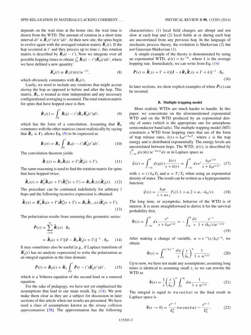
Multiple Trapping Model Multiple Hopping Model

each hop is independenthops are correlated

k(ε) = k0eε/kT , with ε < 0

εt

ε

g(ε)

Miller-Abrahams rates

g(ε)

ε

kij =k0 if εi ≥ εj

k0e(εi−εj)/kBT if εi < εj

FIG. 2. (Color online) Depictions of multiple trapping (left) andhopping (right) models. Each hop in the multiple trapping model isindependent of its previous hops. We call this uncorrelated hopping.By its very nature then, the local fields felt by the spin are alsoindependent at each hop. The multiple hopping models includescorrelations. For instance, a carrier beginning high in energy (asshown) will tend to cascade downwards in energy when operatingunder the Miller-Abrahams hopping rates. Since sites are correlated,the local fields are also correlated, which can be important when aspin hops back and forth between a small number of sites.

10 000–50 000). A single disorder configuration possesses afixed landscape of site energies and local fields.

The relevance of correlations (especially for high disorder)for spin transport as opposed to charge transport can beunderstood by examining site revisitation effects. Carriersoscillate between a small number of sites many times thoughthese sites tend to be near in energy to one another andtherefore the oscillations are rapid and do not contribute to thecurrent [40]. These oscillations are still spin changing eventsthough and hence can be important for spin relaxation and spindiffusion [41].

Though beyond the scope of this article, correlation effectshave been incorporated into CTRW theories on conductiv-ity [47]. Applying these methods to the spin diffusion andrelaxation problem will be a challenging endeavor for theorists.

III. THE δg MECHANISM FOR SPIN DEPHASING ANDSPIN DECOHERENCE

For simplicity, we consider only isotropic g values such thatthe g tensor can be written as g = g I , where g is a randomvariable drawn from a Gaussian distribution centered at g∗with width �g. For this case, longitudinal spin relaxation doesnot exist for this mechanism, so we only examine transversespin decoherence. At a given site i, the total angular frequencyis expressed as ωi = ω0 + δωi , where

ω0 = g∗ μB

�B0x, δωi = δgi

μB

�B0x, (26)

with B0 being the applied field and δgi being the randomvariable taken from a Gaussian distribution centered at 0 andwith standard deviation �g. It is mathematically advantageousto transform to a coordinate system rotating at −ω0 such thatthe effective angular frequency in the coordinate system at anysite is simply δωi . The spin evolution in the new coordinatesystem (marked by a prime) is

dS′(t)dt

= δω × S′(t). (27)

The rotation matrix can be readily found and averaged overthe Gaussian distribution of δgs. The result is

Rs =⎛⎝1 0 0

0 e−a2t2/2 00 0 e−a2t2/2

⎞⎠ , (28)

where a2 = (�gμBB0/�)2. In the absence of hopping, thepolarization is simply P(t) = Rs z; the transverse polarizationdecays in a Gaussian fashion, which has been observed inquantum dots and nanocrystals [42,43]. In the context of elec-tron spin resonance (ESR) experiments, we label 1/T ∗

2 = a.The line width is Gaussian with width �B1/2 = �gB0/2 [44].It should be remembered that this reduction of polarization is aform of inhomogeneous dephasing or broadening and the spinpolarization can be recovered by spin echo experiments.

A. The δg mechanism for spin decoherence

Once the spins begin to hop, the polarization loss isirreversible, which is the scenario we examine now. Using

115203-4

SPIN RELAXATION IN MATERIALS LACKING COHERENT . . . PHYSICAL REVIEW B 90, 115203 (2014)

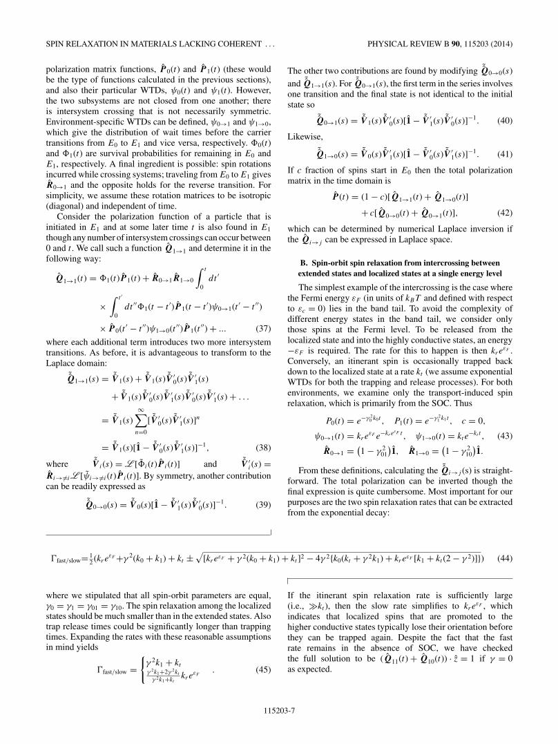
100

1000

Multiple Trapping Monte Carlo simulation

numerical solutions

analytic approximations

10.1 10

0.001

0.01

0.1

1

k0/a = 10

α = T/T0

1/T

∗ 2

FIG. 3. (Color online) Transverse spin relaxation or decoherencerate (in units of a) at long times as a function of disorder. Dottedlines are the analytic result for γ , Eq. (31). Solid lines are thenumerical solution. Blue solid symbols are fit results from a MonteCarlo simulation of the multiple trapping model. As α (a) increases(decreases), the rate approaches the motional narrowing limit, a/k0,which is expected in the case of low disorder. Black symbols: resultfrom the multiple hopping model via Monte Carlo simulations.Multiple trapping and hopping models agree well (indistinguishablein plot) except in the low disorder limit of high α.

Eq. (28), reduces Eq. (14) to the scalar equation

Pz(s) = Rzz0 (s)

1 − R′zz0 (s)

. (29)

The apparent simplicity of this reduced equation is deceiving.The reason is that we are not dealing with R′zz

0 (s) ∝ ψ(s)but instead L [ψ(t) exp(−a2t2/2)], which resists an analyticexpression (for WTDs other than the exponential). ThisLaplace transform is

L [ψ(t) exp(−a2t2/2)]

=∫ 0

−∞

√π2 k0e

(k0ex/α+s)2

2a2 +( 1α+1)xerfc

(k0e

x/α+s√2a

)a

dx, (30)

where x = ε/kBT0. Using this in Eq. (29), the denominatoryields only a single pole, which dictates that the spin relaxationis exponential at larger times. The pole, which corresponds tothe decay rate, can be obtained numerically and is shown asthe solid curves in Fig. 3. The exact pole can be approximatedby expanding the denominator to first order in s and solvingfor s. The inverse Laplace transform yields a decay rate

I1 − 1

I2, (31)

where by using q = ex/α ,

I1 =∫ 1

0

α

(√π2 k0q

αek20q2

2a2 erfc(

k0q√2a

))a

dq (32)

and

I2 =∫ 1

0

αk0qα

(√2πk0qe

k20q2

2a2 erfc(

k0q√2a

)− 2a

)2a3

dq, (33)

Monte Carlo simulations

Multiple TrappingMultiple Hopping

α =12

k0/a = 1000

0 1 2 3 4 5 60.0

0.2

0.4

0.6

0.8

1.0

a t

Pt

0 1 2 3 4 5

0.02

0.05

0.10

0.20

0.50

1.00

a t

Pt

FIG. 4. (Color online) Spin polarization function vs time asdetermined by Monte Carlo simulations. In the disordered case(α < 1), the multiple trapping model agrees well with the morerealistic multiple hopping model. Short times possess a Gaussiantype decay while longer times exhibit exponential relaxation. (Inset)Plot on logarithmic scale showcasing exponential decay at longertimes.

which can be written in close form in terms of generalizedhypergeometric functions. As seen in Fig. 3 (dotted curves),the adequacy of the approximation hinges on the value of α; asα gets smaller than unity, the approximation is completelyinadequate. In the limit of fast hopping/low disorder, thedecoherence rate, Eq. (31), approaches the motional narrowingvalue of 1/T ∗

2 = a2/k0. Lastly, Fig. 3 also shows the resultsfrom fitting the Monte Carlo simulation of the multipletrapping problem (blue solid symbols). The agreement inrelaxation rates between the simulation (multiple hoppingmodel) and theory (multiple trapping model) is very goodexcept in the regime of low disorder where site revisitationeffects are important. The next section discusses this topic ingreater detail.

An example of the polarization function’s shape is shownin Fig. 4. For the slowest hopping/largest disorder, the polar-ization decays in a Gaussian fashion as Eq. (28) makes clear.As the hopping rate is continually increased or the disorder de-creased, the polarization function develops more exponentialcharacter until the motional narrowing regime is obtained.

B. The role of correlations

In light of Fig. 3, we see that the difference between the mul-tiple hopping and trapping calculations is minimal at interme-diate to large disorder strengths (α � 1) for the hopping k0 =1000a (the same is true for smaller k0 also). In this regime,correlations between site energies and local fields must beinconsequential. The reason for this is the following: for largedisorder, wait times are typically longer than the local fieldperiod such that τha � 1. The transverse spin ensemble thendecoheres on a time scale of the order of 1/a, which is what weobserve to be happening in Fig. 3. Whether a spin is frequentinga site often is irrelevant since the phase of the spin is random-ized by the time it embarks on its first hop. The same reasoningcan be used to explain the equivalence of multiple hopping andtrapping models when calculating hyperfine spin relaxation.

The discrepancy between the multiple hopping and trappingmodels is largest when disorder is small and hopping is rapid

115203-5

N. J. HARMON AND M. E. FLATTE PHYSICAL REVIEW B 90, 115203 (2014)

(e.g., at α = 10 in Fig. 3). Since spin decoherence times aremuch longer in this regime, the role of correlations is largerand apparent. Rotations in one dimension (only consideringtransverse decoherence here) commute. So returning to aparticular site one time (each stay being of length τi andτj ) is equivalent to having stayed at the site for a durationτi + τj and not returned to it. From the theory of randomwalks, the mean number of visits to each site of a simple cubiclattice is 1.516 [31,45]. The mean wait time is increased bythis amount 1/k0 → 1.516/k0 [46]. The motional narrowingspin relaxation rate is modified to be 1/T ∗

2 = 1.516a2/k0. Ourmultiple hopping simulations recover this result in the lowdisorder limit as shown at α = 10 in Fig. 3 (black symbol).

IV. SPIN-ORBIT SPIN RELAXATION

Each hop brings about a sudden spin rotation given bythe rotation matrix of Eq. (4) except that now the rotationangles are independent of time; this fact simplifies the math-ematics considerably. For simplicity, we make the followingassumption: the spin-orbit field components are distributed asa Gaussian function with width γ [48]. For the MT model,we are interested in the spatially averaged Rh which, giventhe assumed isotropy of the spin-orbit fields, is proportionalto the identity matrix. In the small angle approximation, theaveraged rotation matrix is simply

Rh = (1 − γ 2)1. (34)

Equation (14) then reduces to a more manageable form:

Pz(s) = �(s)

1 − (1 − γ 2)ψ(s). (35)

For the special case of the exponential WTD, the Laplaceinversion is determined exactly to yield Pz(t) = e−γ 2kt , whichis in agreement with existing theories of spin-orbit spinrelaxation [49,50]. Within the hitherto described multipletrapping model, we can express the polarization in termsof special functions by using Eq. (18). The polarizationin time can be ascertained by numerically inverting theLaplace transform [51–53]. However, in the long-time case,the asymptotic analysis of Sec. II B can be used to find ananalytic expression:

P (t) = 1

�(1 − α)

1

kα0

1

γ 2πα csc(πα)t−α, (36)

which shows that spin polarization is characterized by alge-braic decay [15]. Some physical intuition regarding this resultcan be obtained by noting that P (t) = �(t)/γ 2. By recallingthat �(t) is the probability that a hop has not taken placeup to time t , we see that the polarization decays as carriershop in agreement with what is true from the low-disordercase. Thus the transport of spin is inherently detrimental tospin preservation as expected from the similar Elliott-Yafetmechanism in inorganic semiconductors [1,49].

Figure 5 displays the results of our CTRW theory (blacksolid line from numerical Laplace inversion) and analyticasymptotic expression (dotted line). A large discrepancyappears between the multiple trapping and hopping models,though the qualitative features (algebraic decay) are identical.

MT

MHMonte Carlo

MT (theory)

0 20 40 60 80 1000.0

0.2

0.4

0.6

0.8

1.0

t

Pt

1 10 100 1000 104 105 106

0.02

0.05

0.10

0.20

0.50

1.00

t

Pt

10−3k0t

10− k0t

Eq. 36

3

FIG. 5. (Color online) The spin polarization as a function oftime when relaxation is due to spin-orbit coupling using α = 1/2,γ = 0.025. (Inset) Same data but axes are on a linear scale and thetime scale is shorter. Carriers are injected at sites randomly in thesemiconductor.

Unlike what was found for the δg mechanism, correlations aremuch more pivotal to the SOC mechanism.

The three curves in Fig. 5 depict the full multiple hoppingresult (green symbols), the multiple trapping result (redsymbols and solid black line), and the result where correlatedhopping exists but local fields are uncorrelated (blue symbols).The dramatic differences between the long-time scales of thethree curves indicate the importance of correlated hopping andcorrelated fluctuating fields though the algebraic dependenceis retained in all three.

The indicated results assume spins are injected randomlyinto the amorphous semiconductor (i.e., no site-energy depen-dence). We find that the spin lifetime is contingent on theinjection conditions. For example, if the spins are injectedpreferably to sites lower in energy, the time to decay issignificantly lengthened since the rapid cascading at earlytimes is avoided (not shown). This observation suggests thattuning the spin injection (by a bias perhaps) could alter thespin-relaxation times.

V. SPIN RELAXATION WITH LOCALIZED ANDEXTENDED STATES

Up to this point, we have only concerned ourselves with spinrelaxation for spin carriers hopping within the mobility gap.However, one should also account for scenarios that involvecarriers hopping up to the more conductive states above the mo-bility edge. The CTRW and multiple trapping theories, alreadypreviously introduced here, can be straightforwardly extendedto this more complicated situation. In the following section, wetreat the problem generally where the two subsystems (aboveand below mobility edge) are not yet specified.

A. Spin relaxation of carriers that cross between two systems

Consider two subsystems, E0 and E1, that possess theirindividual set of spin interactions that will lead to spinrelaxation and decoherence, which can be denoted by

115203-6

SPIN RELAXATION IN MATERIALS LACKING COHERENT . . . PHYSICAL REVIEW B 90, 115203 (2014)

polarization matrix functions, P0(t) and P1(t) (these wouldbe the type of functions calculated in the previous sections),and also their particular WTDs, ψ0(t) and ψ1(t). However,the two subsystems are not closed from one another; thereis intersystem crossing that is not necessarily symmetric.Environment-specific WTDs can be defined, ψ0→1 and ψ1→0,which give the distribution of wait times before the carriertransitions from E0 to E1 and vice versa, respectively. �0(t)and �1(t) are survival probabilities for remaining in E0 andE1, respectively. A final ingredient is possible: spin rotationsincurred while crossing systems; traveling from E0 to E1 givesR0→1 and the opposite holds for the reverse transition. Forsimplicity, we assume these rotation matrices to be isotropic(diagonal) and independent of time.

Consider the polarization function of a particle that isinitiated in E1 and at some later time t is also found in E1

though any number of intersystem crossings can occur between0 and t . We call such a function Q1→1 and determine it in thefollowing way:

Q1→1(t) = �1(t) P1(t) + R0→1 R1→0

∫ t

0dt ′

×∫ t ′

0dt ′′�1(t − t ′) P1(t − t ′)ψ0→1(t ′ − t ′′)

× P0(t ′ − t ′′)ψ1→0(t ′′) P1(t ′′) + ... (37)

where each additional term introduces two more intersystemtransitions. As before, it is advantageous to transform to theLaplace domain:

˜Q1→1(s) = ˜V 1(s) + ˜V 1(s) ˜V ′0(s) ˜V ′

1(s)

+ ˜V 1(s) ˜V ′0(s) ˜V ′

1(s) ˜V ′0(s) ˜V ′

1(s) + . . .

= ˜V 1(s)∞∑

n=0

[ ˜V ′0(s) ˜V ′

1(s)]n

= ˜V 1(s)[1 − ˜V ′0(s) ˜V ′

1(s)]−1, (38)

where ˜V i(s) = L [�i(t) P i(t)] and ˜V ′i(s) =

Ri→ =iL [ψi→ =i(t) P i(t)]. By symmetry, another contributioncan be readily expressed as

˜Q0→0(s) = ˜V 0(s)[1 − ˜V ′1(s) ˜V ′

0(s)]−1. (39)

The other two contributions are found by modifying ˜Q0→0(s)and ˜Q1→1(s). For ˜Q0→1(s), the first term in the series involvesone transition and the final state is not identical to the initialstate so

˜Q0→1(s) = ˜V 1(s) ˜V ′0(s)[1 − ˜V ′

1(s) ˜V ′0(s)]−1. (40)

Likewise,

˜Q1→0(s) = ˜V 0(s) ˜V ′1(s)[1 − ˜V ′

0(s) ˜V ′1(s)]−1. (41)

If c fraction of spins start in E0 then the total polarizationmatrix in the time domain is

P(t) = (1 − c)[ Q1→1(t) + Q1→0(t)]

+ c[ Q0→0(t) + Q0→1(t)], (42)

which can be determined by numerical Laplace inversion ifthe Qi→j can be expressed in Laplace space.

B. Spin-orbit spin relaxation from intercrossing betweenextended states and localized states at a single energy level

The simplest example of the intercrossing is the case wherethe Fermi energy εF (in units of kBT and defined with respectto εc = 0) lies in the band tail. To avoid the complexity ofdifferent energy states in the band tail, we consider onlythose spins at the Fermi level. To be released from thelocalized state and into the highly conductive states, an energy−εF is required. The rate for this to happen is then kre

εF .Conversely, an itinerant spin is occasionally trapped backdown to the localized state at a rate kt (we assume exponentialWTDs for both the trapping and release processes). For bothenvironments, we examine only the transport-induced spinrelaxation, which is primarily from the SOC. Thus

P0(t) = e−γ 20 k0t , P1(t) = e−γ 2

1 k1t , c = 0,

ψ0→1(t) = kreεF e−kr e

εF t , ψ1→0(t) = kte−kt t , (43)

R0→1 = (1 − γ 2

01

)1, R1→0 = (

1 − γ 210

)1.

From these definitions, calculating the ˜Qi→j (s) is straight-forward. The total polarization can be inverted though thefinal expression is quite cumbersome. Most important for ourpurposes are the two spin relaxation rates that can be extractedfrom the exponential decay:

�fast/slow= 12 (kre

εF +γ 2(k0 + k1) + kt ±√

[kreεF + γ 2(k0 + k1) + kt ]2 − 4γ 2{k0(kt + γ 2k1) + kreεF [k1 + kt (2 − γ 2)]}) (44)

where we stipulated that all spin-orbit parameters are equal,γ0 = γ1 = γ01 = γ10. The spin relaxation among the localizedstates should be much smaller than in the extended states. Alsotrap release times could be significantly longer than trappingtimes. Expanding the rates with these reasonable assumptionsin mind yields

�fast/slow ={

γ 2k1 + kt

γ 2k1+2γ 2kt

γ 2k1+ktkre

εF. (45)

If the itinerant spin relaxation rate is sufficiently large(i.e., �kt ), then the slow rate simplifies to kre

εF , whichindicates that localized spins that are promoted to thehigher conductive states typically lose their orientation beforethey can be trapped again. Despite the fact that the fastrate remains in the absence of SOC, we have checkedthe full solution to be ( Q11(t) + Q10(t)) · z = 1 if γ = 0as expected.

115203-7

N. J. HARMON AND M. E. FLATTE PHYSICAL REVIEW B 90, 115203 (2014)

VI. AMORPHOUS INORGANIC SEMICONDUCTORS

The theory just outlined is now applied to the case ofspin-polarized carriers in amorphous semiconductors. In thissection, the basic properties of these materials are summarized.In the following sections, we compare the result of the theoryto available ESR experiments.

Transport properties of amorphous semiconductors arecharacterized by two mobility edges at energies, εv andεc, outside of which states are extended (but still unlikeBloch waves) and between which states are localized. Theselocalized states are said to fall within the “mobility gap” ofthe amorphous semiconductor. (Refer to Fig. 6.) The localizedstates are intrinsic to the semiconductor and not necessarily theresult of impurities. There are two types of defect states in purea-Si: dangling bonds that lie near the center of the band gapand band tail states that are formed from the distorted nature ofthe lattice by way of variations in bond lengths, bond angles,and dihedral angles. The former energy states are believed tovary not nearly as rapidly as the latter tail states which possess,near the mobility edges, a density of these states exponential innature [54]. For example, below εc these so-called “band-tail”states are given by

g(ε) = 1

kBT0eε/kBT0 , (46)

where kB is Boltzmann’s constant, T0 is the distribution’s widthin degrees Kelvin and a measure of the disorder, and energyε is taken to be negative. An analogous expression exists forthe valence band tail density of states. Typical values for T0

are in the range of 300–600 K; T0 varies between the valenceand conduction mobility edges and tends to be larger for thevalence-band tail. We assume the dangling bond density ofstates is approximately constant [23,55].

Commonly, the Fermi energy lies within the mobility gap;we assume electron majority carriers though the theory appliesequally well to hole majority carriers. Pure a-Si possesses alarge dangling bond density of states which effectively pinsthe Fermi level near mid band gap, which ultimately makesthe electronic properties of these materials immune to doping.By passivating the dangling bonds through the incorporationof hydrogen, the density of mid gap states is reduced and the

density of states, g(ε)

εv εc

ε

mobility gap

dangling bonds

band tail band tail

conduction bandvalence band

FIG. 6. (Color online) Density of states for a-Si.

hydrogenated material, a-Si:H, can be successfully either p orn doped. Amorphous silicon is prepared through a variety ofmethods, the most prevalent being plasma-enhanced chemicalvapor deposition (PECVD). In this process, silane (SiH4) canbe added whose hydrogens eventually passivate a portion ofthe silicon dangling bonds. Additionally, PECVD allows forthe incorporation of phosphine (PH3) and diborane (B2H6),which lead to n doping from phosphorous and p doping fromboron. The superior properties of a-Si:H led to the materialbeing utilized in electronic devices.

A. Spin properties

Amorphous semiconductors such as a-Si and a-Ge alsocontain few nuclear spins so we can reasonably expectSOC to be limiting. Their hydrogenated counterparts (a-Si:Hand a-Ge:H) do obviously have significantly more nuclearmoments though the observed affect on the ESR line widthis surprisingly minimal, which indicates the paramagneticdangling bonds are well isolated from the hydrogen and arehighly localized on the silicon atoms [56]. For these reasons,we will not further explore hyperfine induced spin relaxation inthis paper. IS mechanisms, which are independent of mobility,have been studied in some detail in the past [57] but will notbe delved into here as our focus is on transport-induced spinrelaxation, which is often observed to be the dominant sourceof spin relaxation at room temperature.

Additionally, the heavier elements present (Si and Ge)suggest SOC effects to be greater than that found in organicmaterials. The SOC strength of γ ≈ 0.1 has been used oftenin the literature. This value is about threes time larger thanthat found for the often studied Alq3 organic semiconduc-tor [50,58]. The larger SOC also gives rise to inhomogeneousg factors, which can dephase or decohere spins in an appliedfield. This effect—which has been considered negligible inorganic semiconductors—has been observed to contributesignificantly to ESR linewidths in amorphous semiconductorsbelow room temperature [24,59].

In the following sections, we discuss spin relaxation inthree regimes of inorganic semiconductors (specifically a-Si ora-Si:H): (1) hopping within dangling bond states, (2) hoppingwithin band tail states, and (3) trapping and activation aboveand below the mobility edges at εv or εc. Low occupationalprobabilities and low spin injection densities allow us toassume dilute carriers and avoid complicating features suchas dipolar and exchange interactions [56,59–61].

B. Undoped a-Si

In undoped a-Si, the Fermi energy lies near mid bandgap within a large density of states coming from danglingbonds. Charge transport in this regime occurs via variablerange hopping [62]. Using the results of Sec. III and theobserved linewidth, �B1/2 = �gB0/2 = 7.5 G, where B0 isthe field corresponding to a resonant frequency of 9 GHz, a�g ≈ 5 × 10−3 is ascertained [44,63,64]. The temperature-dependent portion in Fig. 7 is found from our nondispersiveresult in Sec. IV, 1/T2 = γ 2k(T ), which is a result first realized

115203-8

SPIN RELAXATION IN MATERIALS LACKING COHERENT . . . PHYSICAL REVIEW B 90, 115203 (2014)

100 500200 3001500

2

4

6

8

10

12

20

2

3

5

T K

H1

2G

undoped a-Si

δg

SOC

FIG. 7. (Color online) Black solid symbols are experiments ofRefs. [22] and [23]. Red solid line is our theoretical result. Parametersused: γ = 0.1, k0 = 1010 ns−1, T0 = 4.8 × 107 K. Other experimen-talists have seen the same variable range hopping dependence forlinewidth [60].

by Movaghar and Schweitzer in Ref. [23]. The dangling bonddensity of states is slowly varying around the Fermi level sok(T ) = k0 exp[−(T/T0)1/4] under the assumption of variablerange hopping within a constant density of states. Relaxationtimes in this regime are on the order of one nanosecond atroom temperature.

C. p-doped a-Si:H (trapping and releasing aroundthe mobility edge)

Using the slow rate of Eq. (45) yields a rate 1/T2 ≈kr exp(�E) if k1 � kt , which is shown in Fig. 8 alongwith experimental data on p-doped a-Si:H. We have used ageneric activation �E instead of εF because in actuality themobility edge is ambiguously defined due to the existence oflong-ranged electrostatic potentials from negatively chargedacceptors, which effectively shift the Fermi level by someamount; knowledge of the Fermi level is also obscured by itstemperature dependence [54,65,66]. These ambiguities aside,independence of the spin relaxation to the SOC and the fasthopping rate k1 indicate that the spin relaxation is controlledby the release of carriers from the slowly relaxing localizedstates to the fast relaxing itinerant states.

Another mechanism that could play a role is fast spinexchange between localized and extended states even if theextended states are sparsely populated [55,66,68,69]. We donot investigate this process here.

D. Doped a-Si:H (transport in band tail)

Lastly, we consider doped a-Si:H such that the Fermilevel lies in either the conduction or valence band tail (i.e.,exponential density of states). The theory described in previoussections dealing with an exponential density of states assumeda dilute limit of carriers, which is the scenario present in time-of-flight (and spin injection) experiments where dispersivetransport is observed. This assumption was also implicit inour simulations of a carrier hopping among completely emptystates. A feature of this system, and one that distinguishes itfrom a faster decaying density of states, is that the averageenergy of the carrier continually dives in energy [70]. Thealgebraic spin relaxation predicted herein may be difficult to

p-doping :[B2H6][SiH4]

= 2 × 10−3

a-Si:H

2.0 2.5 3.0 3.5 4.0

0.5

1.0

5.0

10.0

50.0

100.0

500 400 350 300 250

20

100

1

5

0.1

103 T 1 K

Hpp

G

T K

T2

ns

1T2

= 1.7321πg∗μB ΔHpp

FIG. 8. (Color online) Black solid symbols are experiments ofRefs. [67] and [55] as reported in Ref. [66]. Red solid line is ourtheoretical result using the slow relaxation rate of Eq. (45) usingkr = 9 × 102 ns−1 and �E = −0.23 eV.

measure for the following reasons: the slow relaxation willbe masked by other faster mechanisms; in real systems spin-spin interactions between charges must be accounted—theexchange between quasistationary spins and faster hoppingspins will tend to reduce the breadth of relaxation times thatgive rise to the algebraic decay [65].

In real systems, carriers dive until they eventually reachenergies near the Fermi level in which case occupation effectsnow play a role [71]. In these equilibrium situations, the WTDsused in our theory must be defined with care taken to theoccupation of states [10,72]. Such calculations are beyond thescope of this paper.

VII. CONCLUSIONS

We have presented a continuous-time random walk theoryof spin relaxation that is applicable in a variety of systems thatdisplay incoherent charge transport. The theory can accountfor any number of relaxation mechanisms though we havechosen to focus particularly on the relaxation emanating fromspin-orbit effects in inorganic semiconductors. When applyingthe model to amorphous semiconductors, we find excellentagreement with ESR data. Our random walk theory alsopredicts new spin relaxation regimes (algebraic spin decay) forcharge transport within amorphous semiconductor band tails.

ACKNOWLEDGMENTS

This work was supported in part by C-SPIN, one of sixcenters of STARnet, a Semiconductor Research Corporationprogram, sponsored by MARCO and DARPA.

115203-9

N. J. HARMON AND M. E. FLATTE PHYSICAL REVIEW B 90, 115203 (2014)

[1] Y. Yafet, Solid State Phys. 14, 2 (1963).[2] F. Meier and B. P. Zachachrenya, Optical Orientation: Mod-

ern Problems in Condensed Matter Science (North-Holland,Amsterdam, 1984), Vol. 8.

[3] Spin electronics, edited by M. Ziese and M. J. Thornton,Lecture Notes in Physics Vol. 569 (Springer-Verlag, Heidelberg,2001).

[4] Semiconductor Spintronics and Quantum Computation, editedby D. D. Awschalom, N. Samarth, and D. Loss (Springer Verlag,Heidelberg, 2002).

[5] N. Samarth, Solid State Phys. 58, 1 (2004).[6] A. Abragam, Principles of Nuclear Magnetism (Oxford Science

Publications, New York, 1961).[7] C. P. Slichter, Principles of Magnetic Resonance (Harper and

Row, New York, 1996).[8] V. Dediu, M. Murgia, F. C. Matacotta, C. Taliani, and

S. Barbanera, Solid State Commun. 122, 181 (2002).[9] Z. H. Xiong, D. Wu, Z. V. Vardeny, and J. Shi, Nature (London)

427, 821 (2004).[10] P. A. Bobbert, W. Wagemans, F. W. A. van Oost, B. Koopmans,

and M. Wohlgenannt, Phys. Rev. Lett. 102, 156604 (2009).[11] V. A. Dediu, L. E. Hueso, I. Bergenti, and C. Taliani, Nat. Mater.

8, 707 (2009).[12] T. D. Nguyen, G. Hukic-Markosian, F. Wang, L. Wojcik,

X.-G. Li, E. Ehrenfreund, and Z. V. Vardeny, Nat. Mater. 9,345 (2010).

[13] W. J. Baker, T. L. Keevers, J. M. Lupton, D. R. McCamey, andC. Boehme, Phys. Rev. Lett. 108, 267601 (2012).

[14] J. Rybicki, R. Lin, F. Wang, M. Wohlgenannt, C. He, T. Sanders,and Y. Suzuki, Phys. Rev. Lett. 109, 076603 (2012).

[15] N. J. Harmon and M. E. Flatte, Phys. Rev. Lett. 110, 176602(2013).

[16] Organic Spintronics, edited by Z. V. Vardeny (CRC Press,Heidelberg, 2010).

[17] C. J. Cochrane and P. M. Lenahan, J. Appl. Phys. 112, 123714(2012).

[18] P. I. Tamborenea, D. Weinmann, and R. A. Jalabert, Phys. Rev.B 76, 085209 (2007).

[19] G. A. Intronati, P. I. Tamborenea, D. Weinmann, and R. A.Jalabert, Phys. Rev. Lett. 108, 016601 (2012).

[20] A. F. Zinovieva, A. V. Dvurechenskii, N. P. Stepina, A. I.Nikiforov, A. S. Lyubin, and L. V. Kulik, Phys. Rev. B 81,113303 (2010).

[21] A. F. Zinovieva, N. P. Stepina, A. I. Nikiforov, A. V. Nenashev,A. V. Dvurechenskii, L. V. Kulik, M. C. Carmo, and N. A.Sobolev, Phys. Rev. B 89, 045305 (2014).

[22] U. Voget-Grote, J. Stuke, and H. Wagner, in Proceedings of theInternational Topical Conference Structure and Excitations inAmorphous Solids, Williamsburg, VA, AIP Conf. Proc. 31 (AIP,Melville, NY, 1976), p. 91.

[23] B. Movaghar and L. Schweitzer, Phys. Stat. Sol. (b) 80, 491(1977).

[24] B. Movaghar, L. Schweitzer, and H. Overhof, Phil. Mag. B 37,683 (1978).

[25] S. Pramanik, C. G. Stefanita, S. Patibandla, S. Bandyopadhyay,K. Garre, N. Harth, and M. Cahay, Nature Nanotechnology 2,216 (2007).

[26] M. Grunewald, M. Wahler, F. Schumann, M. Michelfeit,C. Gould, R. Schmidt, F. Wurthner, G. Schmidt, andL. W. Molenkamp, Phys. Rev. B 84, 125208 (2011).

[27] A. J. Drew, J. Hoppler, L. Schulz, F. L. Pratt, P. Desai,P. Shakya, T. Kreouzis, W. P. Gillin, A. Suter, N. A. Morley,V. K. Malik, A. Dubroka, K. W. Kim, H. Bouyanfif, F. Bourqui,C. Bernhard, R. Scheuermann, G. J. Nieuwenhuys, T. Prokscha,and E. Morenzoni, Nat. Mater. 8, 109 (2009).

[28] T. D. Nguyen, E. Ehrenfreund, and Z. V. Vardeny, Science 337,204 (2012).

[29] Y. Zhang, T. K. Basel, B. R. Guatam, X. Yang, D. J. Mascaro,F. Liu and Z. V. Vardeny, Nat. Commun. 3, 1043 (2012).

[30] Y. Wang, N. J. Harmon, K. Sahin-Tiras, M. Wohlgenannt, andM. E. Flatte, Phys. Rev. B 90, 060204(R) (2014).

[31] E. W. Montroll and G. H. Weiss, J. Math. Phys. 6, 167 (1965).[32] H. Scher and M. Lax, Phys. Rev. B 7, 4491 (1973).[33] H. Scher and E. W. Montroll, Phys. Rev. B 12, 2455 (1975).[34] G. Pfister and H. Scher, Adv. Phys. 27, 747 (1978).[35] A. Jakobs and K. W. Kehr, Phys. Rev. B 48, 8780 (1993).[36] B. Hartenstein, H. Bassler, A. Jakobs, and K. W. Kehr, Phys.

Rev. B 54, 8574 (1996).[37] CTRW differs from standard random walk theory in that steps

do not occur at a single fixed interval.[38] R. S. Hayano, Y. J. Uemura, J. Imazato, N. Nishida, T. Yamazaki,

and R. Kubo, Phys. Rev. B 20, 850 (1979).[39] J. Klafter and I. M. Sokolov, First Steps in Random Walks

(Oxford University Press, New York, 2011).[40] D. Mendels and N. Tessler, J. Phys. Chem. C 117, 24740 (2013).[41] R. C. Roundy and M. E. Raikh, Phys. Rev. B 88, 205206 (2013).[42] J. A. Gupta, D. D. Awschalom, X. Peng, and A. P. Alivisatos,

Phys. Rev. B 59, R10421 (1999).[43] J. A. Gupta, D. D. Awschalom, A. L. Efros, and A. V. Rodina,

Phys. Rev. B 66, 125307 (2002).[44] R. A. Street, Hydrogenated Amorphous Silicon (Cambridge

University Press, Cambridge, 1991).[45] R. Czech, J. Chem. Phys. 91, 2498 (1989).[46] R. Czech, J. Chem. Phys. 91, 2506 (1989).[47] M. F. Shlesinger, Solid State Commun. 32, 1207 (1979).[48] In Ref. [15], we assumed a constant spin-orbit magnitude and

random angle. Our current formulation introduces a factor ofthree from our prior treatment.

[49] R. J. Elliott, Phys. Rev. 96, 266 (1954).[50] Z. G. Yu, Phys. Rev. Lett. 106, 106602 (2011).[51] P. P. Valko and J. Abate, Comput. Math. Appl. 48, 629

(2004).[52] J. Abate and P. P. Valko, Int. J. Numer. Meth. Engng. 60, 979

(2004).[53] Numerical inverse Laplace transform MATHEMATICA packages

can be located at http://library.wolfram.com/infocenter/Demos/4738/ and http://library.wolfram.com/infocenter/MathSource/5026/ for the GWR and Talbot methods respectively. We findthat the Talbot algorithm typically delivers more stable results.

[54] W. Fuhs, in Charge Transport in Disordered Solids, edited byS. Baranovski (Wiley, 2006), pp. 97–147.

[55] H. Dersch, J. Stuke, and J. Beichler, Phys. Stat. Sol. (b) 107,307 (1981).

[56] P. C. Taylor, in Semiconductors and Semimetals: HydrogenatedAmorphous Silicon Part C, edited by J. I. Pankove (AcademicPress, 1984), vol. 21, pp. 99–154.

[57] M. Stutzmann and D. K. Biegelsen, Phys. Rev. B 28, 6256(1983).

[58] Z. G. Yu, Phys. Rev. B 85, 115201 (2012).[59] D. K. Biegelsen, Solar Cells 2, 421 (1980).

115203-10

SPIN RELAXATION IN MATERIALS LACKING COHERENT . . . PHYSICAL REVIEW B 90, 115203 (2014)

[60] R. Bachus, B. Movaghar, L. Schweitzer, and U. Voget-Grote,Phil. Mag. B 39, 27 (1979).

[61] Z. G. Yu, Phys. Rev. Lett. 111, 016601 (2013).[62] P. Thomas and J. C. Flachet, J. Phys. Colloques 42, 151

(1981).[63] Y. H. Lee and J. N. Corbett, Phys. Rev. B 8, 2810 (1973).[64] P. A. Thomas, M. H. Brodsky, D. Kaplan, and D. Lepine, Phys.

Rev. B 18, 3059 (1978).[65] H. Overhof and W. Beyer, Phil. Mag. B 42, 433 (1981).

[66] H. Overhof, Phys. Stat. Sol. (b) 110, 521 (1982).[67] H. Dersch, J. Stuke, and J. Beichler, Phys. Stat. Sol. (b) 105,

265 (1981).[68] D. Pines, J. Bardeen, and P. Slichter, Phys. Rev. 106, 489 (1957).[69] G. Feher and E. A. Gere, Phys. Rev. 114, 1245 (1959).[70] S. D. Baranovskii, Phys. Stat. Sol. (b) 251, 487 (2014).[71] J. O. Oelerich, D. Huemmer, and S. D. Baranovskii, Phys. Rev.

Lett. 108, 226403 (2012).[72] P. A. Bobbert (unpublished).

115203-11