Det här verket har digitaliserats vid Göteborgs universitetsbibliotek och är fritt att använda. Alla tryckta texter är OCR-tolkade till maskinläsbar text. Det betyder att du kan söka och kopiera texten från dokumentet. Vissa äldre dokument med dåligt tryck kan vara svåra att OCR-tolka korrekt vilket medför att den OCR-tolkade texten kan innehålla fel och därför bör man visuellt jämföra med verkets bilder för att avgöra vad som är riktigt.

Th is work has been digitized at Gothenburg University Library and is free to use. All printed texts have been OCR-processed and converted to machine readable text. Th is means that you can search and copy text from the document. Some early printed books are hard to OCR-process correctly and the text may contain errors, so one should always visually compare it with the ima-ges to determine what is correct.

01

23

45

67

89

1011

1213

1415

1617

1819

20������������������������������������������������21

2223

2425

2627

2829

CM

INSTITUTE OF FRESHWATER RESEARCH, DROTTNINGHOLMREPORT No 29

FISHERY BOARD OF SWEDEN

ANNUAL REPORTFOR THE YEAR 1948

AND

SHORT PAPERS

LUND 1949CARL BLOMS BOKTRYCKERI A.-B.

INSTITUTE OF FRESH-WATER RESEARCH, DROTTNINGHOLMREPORT No 29

FISHERY BOARD OF SWEDEN

ANNUAL REPORTFOR THE YEAR 1948

AND

SHORT PAPERS

LUND 1949CARL BLOMS BOKTRYCKERI A.-B.

Table of Contents

Director’s report for (he year 1948; Sven Runnström ............................................................. 5Short papers:Influence of heredity and environment on various forms of trout; Gunnar Aim .... 29Movements and growth of grayling; Karl-Jakob Gustafson ..................................................... 35Predators on salmon fry in the river Mörrumså in 1948; Jöran Huit and Alf Johnels . . 45Vitality of salmon parr at low oxygen pressure; Arne Lindroth ........................................ 49Étude quantitative des planctons crustacés dans quelques lacs du Jämtland; Thorolf

Lindström ........................................................................................................................................ 51

Fertility of char (Salmo alpinus L.) in the Faxälven water system, Sweden; AlexanderMäär .................................................................................................................................................. 57

Experiments in Lake Väner on the influence on fish of bomb-dropping; Carl Puke . . 71A new water sampler; Carl Puke........................................................................................................ 75

Bottom fauna and environmental conditions in the littoral regions of lakes; Carl Puke 77Environment and productivity of the lakes near Stockholm; Carl Puke ....................... 81Control of trout migration by a fish ladder; Sven Runnström ............................................ 85The Coregonid problem. I. Some general aspects of the problem; Gunnar Svärdson .... 89Note on spawning habits of Leuciscus erythrophthalmus (L.), Abramis brama (L.)

and Esox lucius L.; Gunnar Svärdson .............................................................................. 102Competition between trout and char (Salmo trutta and S. alpinus) ; Gunnar Svärdson 108Salmon (Salmo salar L.) with no adipose fin; Gunnar Svärdson ................................... 112Natural selection and egg number in fish; Gunnar Svärdson ............................................ 115Sex differentiation in eel (Anguilla anguilla) and the occurrence of male eels in the

Baltic; Gunnar Svärdson ............................................................................................................ 133

Eels (Anguilla anguilla) found in Sweden in partial nuptial dress; Gunnar Svärdson . . 129Stunted crayfish populations in Sweden; Gunnar Svärdson ................................................ 135Maränenfischerei im Fluss Gimån (Jämtland) ; Hendrik Toots ............................................ 146

Director’s Report for the Year 1948

By Sven Runnström

Introduction

The Institute of Fresh-Water Research, Drottningholm, (formerly: The Swedish State Institute of Fresh-Water Fishery Research) was founded in 1932. The Institute was directly under the Fishery Bureau of the Board of Agriculture with the chief of that Bureau as its director. On July 1st 1948, the Swedish Fishery Board was established, and the Institute’s former director — fil. dr. Gunnar Alm — consequently appointed to the administra­tion of freshwater fisheries within the Board. The Institute now represents fresh-water fishery research within the Board under the supervision of its own director.

During the past years the results of the research have been published as reports appearing at various intervals. A list of all the reports published hitherto is found on the cover of this booklet. Considering the vast amount of research being carried on at present at similar institutes in other countries, it should, however, he of interest to publish an Annual Report, a survey of the year’s work at our Institute and short reports from the staff. More comprehensive work will, however, even in the future appear as separate papers.

Members of the Staff in Jan. 1949

Assistant Secretary:

Director:Fishery Biologists:

Fishery Assistants:

Sven Runnström, fil. dr. Lars Brundin, fil. dr. Gunnar Svärdson, fil. dr. Alexander Määr Thorglf Lindström, fil. lic. Eric Fabricius, fil. mag.K.-J. Gustafson, fil. kand. Gösta Molin Hendrik Toots Arne Johanson Birgit Sandgren

6

Laboratory Assistants: Ingrid JohannissonHelve Toots

Porter: Henning Johanson

Kälarne Research Station (in the province of Jämtland)Fishery Assistant: E. Halvarsson

The following employees of the Fishery Board have also done temporary research work in the laboratory: Gunnar Alm, fil. dr., Chief of the Bureau of Freshwater Fisheries, Elias Dahr fil. dr., Carl Puke fil. lie.

In addition, B. Carlin, fil. dr., the fishery biologist of the Migratory Fish Committe has an office at the Institute.

Scientific and Practical Work by the Staff

Production of Bottom and Plankton Animals

The general aim of the work of the Institute is to investigate the possi­bilities of increasing the fish yield in our lakes and rivers.

The yield of the lakes is mainly determined by the supply of suitable fish food which in its turn depends on the general metabolism of the lakes. It would be beyond the task of the Institute to deal with the first stages of this process, which are more within the sphere of the limnological institutions of the universities. We have, therefore, concentrated more on investigations on the bottom and plankton fauna and its importance as fish food.

The knowledge of our lakes is still very fragmentary, in spite of much scientific work, and this is none the less true of the bottom fauna, so important in practical fishery biology. In 1941—42, when Brundin worked on quantitatively collected material from oligotrophic lakes in northern Sweden, he did not find any fixed points to compare with other Swedish lakes. Earlier scientists had also arrived at contradictory results regarding the influence of the humus standard on the bottom fauna. The almost entire lack of information on the Chironomids in our lakes was also troublesome, as these belong to the most important group of bottom animals. Only by establishing the species represented by the Chironomids, an idea of the relation between the different lake types and the Chironomid fauna can be formed.

In order to solve these problems, Brundin started investigating the bottom fauna in 1942, paying special regard to the Chironomids in the Aneboda- Växjö-sector, which lakes hold a key position in regional limnology, thanks to the works of Naumann and his pupils. Environmental factors have also been better investigated there than in other Swedish lakes.

One of the most important questions was to find out how the humus factor influences the bottom fauna qualitatively as well as quantitatively. In some lakes with different humus standards, series were taken with an

7

Ekman-Birges’ bottom-grab, approximately 23 cm high, during different seasons along cross-sections from the shore to the greatest depth, parallel to the oxygen and temperature series. Special attention was given to the littoral biotopes.

Experiments with a funnel-shaped trap of wire-cloth hanging below the water surface with an upside-down glass bottle attached to the upper smaller hole formed an important complement to the quantitative bottom-grab series. The insect pupas rising from the bottom of the lake are caught in the trap. The hatching then occurs at the surface of the water in the glass bottle. This method gives an idea of the biology and ecology of insects hatching on the surface of the water and elucidates inter alia the following problems.

1. The identity and number of the hatching insects from different bio­topes per day and area unit.

2. The quantitative and qualitative composition of the insect fauna in all bottom biotopes, both organogene and minerogene. This means that direct comparisons can be made between the insect populations of the soft bottoms and the exposed stone and block banks, which is not possible with the other methods used hitherto.

3. The influence of limnic environmental factors on the hatching.Simultaneously with these investigations, considerable material of Chiro-

nomid imagines was collected during different seasons, thus giving an idea of the number of Chironomid species in different types of lakes and the phenologic character of the Chironomid fauna. In order to classify the Chironomid larvae, many of them were hatched by breeding, and it was possible to identify practically all the larvae found in the Småland lakes.

It soon became clear that material from other parts of the country had to be compared with the bottom fauna characteristic of the Småland lakes. A considerable amount of Chironomids, especially imagines, was therefore collected from Skåne to the mountain districts in northern Jämtland. The material from North Sweden was, moreover, supplemented by a valuable and extensive Chironomid material collected by Määr, from mountain lakes in Jämtland.

The material thus collected seems to make general discussion possible on the bottom fauna characteristic of the Swedish oligotrophic lakes. This material has shown that our lakes are populated by more than 300 Chironomid species. There are about 140 Chironomid species in an oligotrophic lake in Southern Sweden of the oligohumous, harmonic type. With increasing humus standard, the number of species decreases, slowly at first, but very quickly within the polyhumous group of lakes. The extremely polyhumous little moss pools have only about 40 species of Chironomids.

Some of the results of the systematic working up of the material have been published in two papers in 1937 and 1938. Thirtyeight of the species found in Swedish lakes were new to science. Four new families are represented, and it

8

has been possible to identify the pupa and larval stage of rather many hitherto unknown species.

A survey of the general results of the lakes investigations is now being worked out, and is to be published this year as report nr 30 from this Institute.

In connection with investigations in such Norrland lakes which are to be impounded during the next few years, Määb has studied closely — both quantitatively and qualitatively — the composition of the bottom fauna in the water courses of Faxälven. The sector investigated comprises a series of 8 lakes, starting in the forest district of Jämtland and ending in the mountain districts above the cultivation limit, 669 m above sea level.

Investigations have been planned to study the changes in the production of the lakes which appear when regulating the water-level. As the bottom fauna is, however, little known in these districts, the research considerably increase our knowledge of the production conditions in the Norrland lakes and supplement Brundin’s investigation in the Småland lakes.

In 1943 and 1944, quantitative bottom samples were collected from 27 permanent bottom profiles. This material was supplemented in 1945—48 by samples collected during different seasons in Blåsjön and Russfjärden. In all, 690 samples have been collected. In 4 of the lakes, tests have also been made with traps shaped like cages, but otherwise constructed like those used by Brundin. This material illustrates the hatching periods of a great number of larvae of Chironomidae, Trichoptera, Ephemeroptera and Diptera. In addition, investigations have been made on the composition of the stone bottom fauna and a great many air insects have been collected. In connection with the bottom investigations, oxygen, pH, water temperature, transparency and colour have been determined and plankton samples taken in all the lakes.

The material is now being worked on, and the first report from Dr. Määr will very likely appear in 1950. One result of the investigation is that the productive littoral zone in the mountain lakes extends rather deeply, which fact may be connected with the great transparency of these lakes. This is of great importance when judging the influence of regulating the water-level on the production of fish-food in the lakes.

C. Puke has worked during the past years on a material, collected over a period of several years, comprising the bottom fauna in Lake Mälar and the lakes around Stockholm. The material comprises both biological and hydrographical samples. The investigations aim partly at studying the littoral fauna and its environmental conditions, and partly at establishing the pro­duction capacity of different types of lakes.

Investigations have also been made by Th. Lindström on the plankton pro­duction in certain parts of the water system of Indalsälven (Storån) in Jämt­land. Quantitative samples have been collected during different seasons with a large water sampler, and the material gives an idea of the seasonal varia-

9

tions and the distribution of the animal plankton at various depths, and an approximative idea of the plankton production of different lakes and in different regions of the same lake. It is of special interest here to study the supply of plankton at the time when the newly hatched fry begin to seek for food.

The Relationship between Food and Fish Production

The above investigations on the production of the lakes are of fundamental importance for a closer study of the relationship between fish and avail­able food. In connection with investigations on the biology of different fish species, a large number of fish stomachs has been collected, which give a general idea of the food of these fish. With the detailed reports from certain lakes on bottom and plankton fauna now at hand, il should be possible to demonstrate the supply of food available, and how this supply is utilized by the fish.

In connection with Määr’s investigations on the bottom fauna in Faxälven, 2,300 stomachs of 8 species of fish were collected. These will be treated as soon as the results of the bottom investigations have appeared. Brun- din will also take up similar problems, and Lindström has started some aquarium experiments regarding the feeding habits of char fry.

When these experiments have clarified the question of the utilization of fish food and the food competition between different species, it will be easier to judge the possibility of exploiting the fish food production of the lakes as much as possible by suitable combination of fish stocks, and thus obtain an optimal production of edible fish. It is already clear that the coarse fishes, which now compete for the food with the more valuable fish species, should be controlled.

It might also be possible to enrich the lower fauna of the lakes with in­vertebrate species, especially suitable for fish food. I mean relict species, such as My sis relicta and others, which exist in certain lakes below the former marine limit. These should be suitable as fish food because of their size, and trout has proved to grow very rapidly in Norwegian Mysis lakes. Mysis relicta also makes use of the otherwise only slightly productive deep zone. This species should find good living conditions in our deep and cold mountain lakes and contribute to the feeding of char and whitefishes. Experiments will be made this year with planting Mysis and possibly other form of relicts in a suitable lake.

The above-mentioned measures might possibly lead to better utilization of the food in the lake from the fishing point of view but it can of course not increase this food which depends chiefly on the supply of nutritive salts, etc. A certain limit will soon be reached when the relation between the fish yield and the food supply is stabilized. A further increase of the fish

10

population will only cause a decrease in the growth of the fishes, which is very variable and depends on the food supply. Stunted fish populations can thus appear as we know from a great number of our lakes, i.e. in the shape of dwarf perch and small whitefish, lakes which must be regarded as unproduc­tive as far as fishing is concerned.

The only way really to increase the supply of food animals and thus the yield of the lakes is to give the lake a further supply of nutritive salts by fertilizers. It would be highly desirable for the Institute to include experi­ments on fertilizing of lakes in its programme. The practical usefulness of this method is, however, determined by the financial gain resulting from it.

Improvement of Lakes by Introduction of New Fish Species

Near Kälarne Research Station (in the province of Jämtland) there are a great number of rather different small and medium sized lakes, but all characteristic of the forest regions in central Norrland. Here Alm has for a several years carried out general hydrographic and fishery biological research in collaboration with the late Tage Borgh. Their work comprised chiefly of determining temperature and oxygen conditions, pH-value, shore and bottom state, and flora and fauna, in connection with experimental fry-planting of already existing and new fish species. The aim is to get a general idea of the production conditions in these lakes, the possibility of utilizing them rationally, and to find out the optimum fish yield, the most suitable fish species, etc. Even though the lakes are generally small, a great number of such lakes are, if rationally cultured, of great importance to the fishery proprieter, both as regards their yield of fish and the opportunities for sport fishing they may offer.

The experiments, which will be carried on for some years more, have already given interesting results. Thus, planting of char (Salvelinus alpinus), trout (Salmo trutta) and whitefish (Coregonus lavaretus) has turned out very well in many of lakes, previously considered as rather unproductive. The first generation of the planted fishes, — sometimes fry, sometimes Engerlings bred in ponds were used — have often shown very good growth in lakes of 5—10 hectares and 6—10 meters depth, pH of 5—6, strongly developed stratification and hypolimnion with very low temperature, partly or quite without oxygen. Whitefish has even propagated in such lakes, in spite of the absence of hard bottom, so that a new generation has grown up. Experiments are now planned to kill dwarf perch populations by poisoning them in order to utilize certain of these lakes for salmon species. Experiments with lime, perhaps also with fertilizers, will be made if possible.

11

Testing the Effectivitg of Artificial Propagation

Plantings of fry or fingerlings have been used for a long time as an important measure for improving the fish yield of our lakes. It is thought that great losses may occur in nature during the egg development and hatching, which can be avoided by artificial fertilization and by breeding the spawn in hatcheries. It would thus be possible to supply the lake with additional fry, resulting in an increased fish stock. We have now a great many hatcheries in our country from which millions of fry are sent out, especially that of pike and whitefish.

The present methods of fish culture need however to be revised, and this will be one of the most important questions in the program of the Institute.

As the food supply of the lakes limits the fish production, and as only two grown-up fishes must result from the spawn laid by one female to keep the population constant, it is probable that a great surplus of fry is produced in lakes with normal spawning possibilities. This results in food competition between individuals of the same stock, while only a few thousendths of the fry develop into mature fishes. Plantings of fry in such lakes would only cause increased competition and mortality. Fish culture can, on the other hand, play an important rôle in new plantings, either in waters without fishes or in lakes where a better combination of the fish stock is desired by introducing a suitable new form and outfishing the less desirable fish species. Fish culture should also fulfill a mission in lakes and rivers, where the natural spawning possibilities are spoiled, i.e. by water-level regulating and impoundments by dams.

In order to consider the financial advantage of fish culture, the Institute has started a comprehensive investigation of this matter, and treated the problem from several angles. The investigations comprise for example varying plantings in connection with statistics of the catching and introduction of fingerlings, marked by cutting of fins, or fry of easily recognizable bastards, or fry otherwise marked in a natural way.

It is natural, that especially the profits from the pike culture which plays a greate rôle in our country, has been subject to critical examination. Svärd­son has investigated the problem in two ways; by experiments during the pike spawning period in the Institute’s own water at Drottningholm, where the spawning frequency is studied in connection with external environ­mental factors. The migration is studied by means of tagging, and fin cut fingerlings are released to find out the effect on the stock. The total number of pikes caught since these research started in 1945 is over 1,000. Scale samples of all fish have been taken, but up to now they have not been worked on.

The second principal line in Svärdson’s pike investigations is an extensive collection of scale samples and fishery statistics from 15 fishermen all over

12

the country. The fishermen have bound themselves by contract to take scale samples and note the size, weight, etc. of each pike caught, for which work they are compensated. This research work was started in 1946 and is to be continued during the next years. No examination of the scale material has been made up to now but the reports have been used as a basis for certain practical considerations as to the average weight of each pike caught of different sex, the selective fishing of different sexes with different tackles, etc. (Svärdson 1948.) In 1948, pike fry were planted at half of these stations, in order to get an idea of the profit measured by increased yield.

As to the char, Runnström has studied the spawning conditions at Torrön and in other Jämtland lakes. The spawning stock and the amount of spawn laid in nature have been estimated approximately. Hatching experiments have also been made in boxes, at the natural spawning places.

At Torrön, where fishery statistics and scale samples have been collected for many years, the char plantings have been under control and have during the last few years only been made every second year. The plantings have also varied as to fry and fingerlings. In 1948 10,000 char fingerlings were planted at Torrön and 5,000 in Blåsjöälven, all of which were marked by cutting of fins. In other regulated char and whitefish lakes, an experimental period has been reserved during which no plantations are to be made, in order to compare the age classes thus arising, with the results from years with release of fry.

In Lake Vätter, which contains a considerable stock of big char, fry from char spawn caught at normally forbidden seasons have been planted for many years but was suspended in 1945 and afterwards. The idea is to compare the results of natural spawning — investigatin the age classes several years after and making exact statistics of the fishing — when fishing is prohibited during the spawning season, and when fry is planted from spawn caught during the spawning.

In order to decide the financial advantage of pike-perch culture, C. Puke has for a couple of years carried on investigations on the pike-perch spawning in Lake Väner, where the fishermen in Dettern have to take part in fish culture, in order to be allowed to fish during the spawning. Experiments have been made to settle the percentages of natural and the artificial fertilizing and hatching, and the natural egg destruction. To get an idea of the fishing intensity and the age composition and to judge whether overfishing occurs, markings have been made and a great number of scale samples collected. This material is now being worked on, but will have to be further completed.

Reports have been given on the marking of fingerlings by cutting fins. These experiments will be further extended this year and the vitality of the marked fishes will also be investigated.

Most plantings are, however, made with newly hatched fry, and there are no possibilities for controlling the results of these by means of marking.

13

Last autumn char and trout were crossed and a great amount of spawn was laid in for hatching. These hybrids are easily recognized from their colour markings and can be used for testing.

This extensive investigation on the financial advantage of fish culture must be regarded as a programme with a distant aim, but as fact accumulate, it will be easier to draw up lines for a more scientific fish culture. The main importance will, as has already been mentioned, be then attached to qualita­tive improvement by new plantings of specially selected fish species in connection with removal of undesired species. Today, little importance is normally attached to the origin of the fry material. When ordering whitefish fry, for example, the receiver will seldom ask what kind of whitefish it is. It will therefore be of great importance to know the quality of the different fish populations as to propagation, food ecology, growth etc.

Mutants in FishDuring last year, Svärdson has found an abnormal, silvercoloured mature

pike, the spawn of which was fertilized with milt from an one-year old male. A F-l generation was thus created consisting of about 50 fishes, which are now being reared. Furthermore, about 40 abnormally light yellow pike fry were found at Fuse by Lindroth, who brought them to the Institute. By special efforts with enormous feeding of plankton, roach fry, etc., these pikes have been raised to unusually big yearlings, 26 of which are still alive. The still visible colour deviation is probably due to a mutant gene; this must however be controlled. Also unusually light coloured fingerlings of char have been isolated at the hatchery of Semlan for further observation. When cutting the fins of salmon fingerlings at Älvkarleby in the autumn of 1948 about 20 fingerlings were found which spontaneously lacked adipose fin. Even this was suspected to be due to mutation or recombination of recessive genes.

The purpose of controlling these colour and morphological deviations is to find out whether they are hereditary and to investigate their vitality, in order possibly to use these fishes in the future for producing innately marked fry, whereby the advantage of plantings of newly hatched fry might be more easily tested.

Control of Fish Populations and the Results of Natural PropagationIn Lake Jormsjö (Jämtland), where the main spawning of the char

takes place in streams, a weir was built in the river during the spawning periods in 1947 and 1948. The spawning stock was controlled here as to number, sex, age composition, spawn number, etc. The fishes were also marked to determine migration and the number of individuals coming back for repeated spawning. The control is to be continued this year under the supervision of Runnström.

14

Runnström is investigating trout at the outlet of Lake Lillrensjö, where a fish ladder has been built in a dam. This outlet is the only spawning place of the trout stock, and all fish migrating down and upstream have been counted, measured and marked. The number of downstream migrating mature fish and that of upstream migrating young fish in summertime has thus been determined. Scale samples have been taken at different seasons so that the growth during the season etc. can be controlled. In addition, in 1947 8,000 fingerlings were planted in the lakes and in 1948 4,000 in the lake and 1,000 in the stream, all marked by cutting a fin in order to compare the result of the natural spawning and the plantings. These experiments will be continued in the present year. Marking tests are also going on with the great trout in Lake Kallsjö, and clearly indicate that individual fishes only spawn every second year. An inventory of certain trout spawning streams by means of electrical fish shocking is also planned this year.

Similar experiments to that with trout in the fish ladder at Lake Lillrensjö are being made in a grayling spawning stream by K. J. Gustafson assisted by Arne Johansson. At a trap built in the mouth of the stream, all upstream migrating mature grayling were examined during the spring of 1948 as to length, weight, sex and age. Marking tests were made to learn about migration, fishing intensity and migration back to the spawning stream. In summer and autumn, downstream migrating young grayling were controlled in a special trap and marked by cutting of fins, partly to find out when catching the fish later if these fishes go back to their native stream for spawning, and partly to obtain the valuable test formed by these fishes of known age for the continuous studies of age and growth on the scales. In a neighbouring stream, 2,000 fin-cut fingerling grayling, bred in ponds, were introduced for comparison with the results in the experimental stream. These investigations of the biology and propagation of the grayling are to be continued during the next few years.

At the so called »vaktfisket» in Lake Idsjö in the water system of Gimån, an interesting whitefish fishery has long since been carried on during the spawning migration upstream. A weir has been built across the stream and is so constructed that the whitefish can pass during the upstream migration, but when migrating downstream after the spawning, it is forced to go through an opening where it is caught. As several townspeople own this fishing, daily notes are made about the fishing, in order to divide the catch. H. Toots has for the two past years collected and worked on material regarding the age composition, growth, sex ratio, etc., of the spawning stock and got statistics over a long period. If carried on for some more years, these in­vestigations should give interesting results as to the changes in growth and strength of the different year classes. Toots has also made tests on the newly laid spawn, using a pump-arrangement of his own construction in order to determine the fertilization percent, and he is to continue taking these

15

samples until the spring in order to study the hatching results etc. Experi­ments with specially constructed traps have also been carried out to see to what extent the spawn is carried away by the stream.

Studies in Spéciation of Fish

Certain fish species are apparently rather constant in different lakes, while other species such as char and whitefish show great variations. Whitefish especially have been a great problem to the taxonomists. The Research Institute has therefore considered it necessary to penetrate the whitefish problem, and investigations are going on under the supervision of Svärdson. As the question is so farreaching, tasks have been divided so that Fabricius, Toots and Johanson, investigate — each in his field — the whitefish forms and then- biology. Collaboration has also been initiated with certain county fishery employees. Svärdson started these investigations as early as the autumn of 1945 by taking fish samples from a lake in the Arjeplog parish, whex-e at least thx-ee species live together. Spawn from two of these has been transferred to the Kälarne Research Station, and after the hatching of the fry, they were placed in two tarns. The growth in this environment has been considerably modi­fied in both cases, compared with that in the original water. As to purely systematic characteristics no analysis has as yet been made, but it can be preliminarily stated that it is still easy to distinguish the two species in then- new environment. During the latter part of 1948, a regional collection of samples from spawning stock in some lakes was made, in order to obtain a survey of the different species of whitefish in our counti-y. This material is now being treated, and a great number of systematic characteristics are being examined. An inventory has also been stai-ted, to record cases of introduction into new lakes where the origin of the stock is known. There are thus new possibilities of comparing the same stock in two environments. Reports have been collected from several cases, and material will be collected dui-ing the spawning season. The opinion of the modem systematics that two fish populations, residing in the same environment, must be regarded as species if complete sexual isolation occurs, has so far been proved at some fry-plantings since obvious differences in spawning habits, have proved to be constant when transfering the species to new environments.

Apparently the char offers the same problem as the whitefish. In the same lake, up to three different forms can appear which differ as regards growth and spawning habits. An extensive char material has been collected from different lakes by Runnström and certain planting experiments have also been made in tarns within the Kälarne experimental area. The material is to be examined this year for further completion. The difficulty with the char is to find suitable systematic characteristics to differentiate the various forms, and special importance will be attached to this matter. Runnström will also

16

continue his studies of the vendace (Coregonus albula) with special regard to the spring spawning species described by him. Grayling is also subject to investigations by Gustafson. It is here of special interest to control the reports collected from different places on a certain autumn spawning grayling species.

At Kälarne Research station, investigations have been carried on for many years under the supervision of Alm on the above mentioned race question in trout and perch, as well as direct experiments on the connection between growth, age and sexual maturity of different fish species. Such experiments on perch were recently continued in order to illustrate and complete the results from Alm’s paper »Reasons of the occurrence of stunted fish-popula­tions» (Report nr 25). The present investigations aim at explaining the strange fact that sexual maturity begins at high age in such cultivated populations displaying a bad growth but at a lower age in spontaneous populations which have the same slow growth rate.

As to trout, Alm has proved before that the different growth and size of small river-trout and large lake-trout almost entirely consists of modi­fications and is determined by the environment, while maturity and some colour designs are hereditary to a certain point. More can be read about this in Report no. 15. When breeding offspring of these two trout forms in ponds, it has now been proved that even in the second generation and probably also in the third, maturity occurs earlier with the offspring of river trout, which also keeps the often strongly marked white and black border colour on ventral and anal fins, while the offspring of lake trout more often occurs without this colour and mature later. Thus the probability that these qualities are hereditary is very great. Investigations are, however, being carried on in this field which aim simultaneously at illustrating the influence of maturity on the growth.

Damage to Fish Stock by Regulating Dams in Lakes

In order to utilize the water supply in the rivers for electric power effi­ciently, great projects are at hand to impound the lakes in the Swedish Norrland rivers. The water can thus be stored during the springflood, and used later during low water periods which occur especially in winter. The Institute carries on investigations in a great number of lakes in northern Sweden to study the influence of the often considerable water level variations on the fish food and the spawning etc. The aim of these investigations is to compensate the damage to the fish-stock as much as possible by means of different measures.

Hydro-Electric Power Dams and Migration of Salmon

Investigations have been started by the Migratory Fish Committee (Alm, Hult and Carlin) to find out suitable and rational measures to compensate

17

damages to the salmon stock by building hydro-electric power dams across the rivers. Scale samples are being collected in order to investigate the strength of the year classes and the age composition of the stock in different fishing years. Experiments have also been carried out on different kinds of fry breeding and salmon has been transferred to such parts of a water system which it could not enter by itself, but which can be used as natural spawning and fry grounds. Tagging of mature salmon has been made and also marking of fingerlings by means of fin cutting. The stomach contents of different small fishes, caught where salmon fry has been planted, have shown that small perch especially is a voracious predator. During the next few years, investigations will aim at finding the most rational and economic methods for breeding salmon fry to migratory size.

Practical Research on Greater Strength of Fish Nets

Apart from the usual routine work in connection with different fisheries the tasks of the fishery assistants comprise at present the following investiga­tions and experiments made by Molin.

Impregnation experiments. Great uncertainty still prevails among fisher­men as to the reliability of the numerous impregnation compounds on the market. In 1948, a series of experiments was started to find out what substances are in general most fit for impregnating fishing gears of coarse and fine nets.

Nylon experiments. Fishing gear made of nylon have up to now not been much used, but since 1948, experiments have been going on to find out if nylon can be used for the manufacture of nets and traps. The early phases of the experiments have comprised calculation of the tensile strength of nylon thread and its strength in relation to cotton thread. Finally, experi­ments are to he made in practical fishing with tackle made of nylon thread.

Library

The Institute subscribes to certain fishery biological and limnological periodicals, and buys some technical literature. Due to the limited budget of the Institute, the library must, however, rely on periodicals, institution publications and reprints which are obtained in exchange for the reports from the Institute. Further exchange of reports and reprints is invited.

Literature

The reports published by the Institute and other articles of general interest for fresh-water problems written by the staff and other members of the Fishery Board are listed below. As an annual report is now published for the first time, it has been considered suitable to refer back to the very beginning of the Institute’s

2

18

activity. The large number of papers written in Swedish are included principally for Scandinavian readers. The most important papers are written in foreign languages or have a summary for readers abroad.

Rep = Report from this Institute.SFT = Svensk Fiskeri Tidskrift (Swedish Fishery Journal). Only Swedish language. SOU = Statens Offentliga Utredningar (Official Deliberations of the Swedish State).

Only Swedish language.

1933

Alm, G. Statens Undersöknings- och Försöksanstalt för sötvattensfisket. Dess till­komst, utrustning och verksamhet. The new Institute of Freshwater-Fisheries at Drottningholm, Sweden (Summary). Rep. 1: 1—24.

— Fiske, fiskerätt och fiskevård i våra sötvatten. Wahlström & Widstrand, Stock­holm. 157 pp.

— Föreningsväsendet på fiskeområdet. SFT 42:41—44.— Minimimått på gädda. SFT 42: 157—159.— Riktlinjer för utökande av sportfiskemöjligheterna på kronans fiskevatten.

Stockholms Sportfiskeklubbs Årsbok: 1—12.— Laxen, en värdefull naturtillgång. Lantbruksstyrelsens flygblad 2: 1—5.— Fiskeribiologiska synpunkter vid delning av fiskevatten. Protokoll hållet vid

Sv. Lantmätareförbundets årsmöte 1933: 18—30.— Die Anstalt für Binnenfischerei bei Drottningholm (Stockholm). Arch. f. Hydro-

biol. 26: 143—146.— Våra sötvattensfiskars föda. Från Skog och Sjö 26: 191—198.

Freidenfelt, T. Untersuchungen über die Coregonen des Wenersees. Int. Rev.gesamt. Hyclrobiol. u. Hydrograph. 30:49—163.

Hessle, Chr. Ålfiskets beroende av vind, ström och månens faser. SFT 42: 145—149.Olofsson, O. Om rommens mängd, antal och storlek hos laxen. SFT 42: 13—16.— Varför äro laxar med lekinärke å fjällen sällsynta? SFT 42: 33—36.— Ett par allmänna stadgefrågor. IV. Tjugo varv på aln. SFT 42: 133—136.— Den torra sommaren och fiskdöden. SFT 42:271—273.— Rommängd och romsvällning hos siken. SFT 42: 277—279.— Några inplanteringar av Lomsjösik. SFT 42: 280—283.

Vallin, S. Cellulosafabrikerna och fisket. SFT 42: 241—248.— Kräftpestens spridning inom Sverige under 1932—1933. SFT 42: 186—190.

1934

Alm, G. Vätterns röding. Fiskeribiologiska undersökningar. Fischereibiologische Un­tersuchungen des Saiblings im See Vättern (Zusammenfassung). Rep. 2: 1—26.

— Salmon in the Baltic Precincts. Rapp, et Proc. Verb. Cons. Perm. Int. l'Explor. de la Mer 92: 1—63.

— Bemerkungen zu der Lachszuchtfrage Rapp, et Proc. Verb. Cons. Perm. Int. l'Explor. de la Mer 91: 17—18.

— Exempel på lyckade fiskinplanteringar. Från Skog och Sjö 27:416—421.— Hushållningssällskapen och fisket. Hushållningssällskapens tidskrift 1: 117—127.— Laxen i Östersjöområdet. Stockholms Sportfiskeklubbs Årsbok: 1—14.— Statistik för sötvattensfisket. SFT 43: 13—15.

Hessle, Chr. Märkningsförsök med gädda i Östergötlands skärgård åren 1928 och 1930. Pike-Tagging in the archipelago of the Swedish Baltic coast, Östergötland (Summary). Rep. 3:1—17.

19

Nybelin, O. En mystisk ålsjukdom i våra sötvatten. SFT 43:205—208.— Rödsjuka hos ål i saltvatten och förebyggande åtgärder mot densamma. Lant-

bruksstyrelsens flygblad 4: 1—4.— Über Agglutininbildung bei Fischen. Zeitschr. f. Immunitätsforschung 84: 74—79.

Olofsson, O. Några inplanteringar av Lomsjösik. SFT 43: 4—8, 16—18, 43—47,74—79.

— För och emot storryssjorna. SFT 43: 172—180.— Försvinner ålen i övre Norrland? SFT 43: 241—243.— Rommängd och romsvällning hos rödingen. SFT 43: 277—279.— Edefors laxfiske. Några drag ur laxfisket och dess historia i Lule älv. Norr­

bottens läns hembygdsförenings årsbok: 47—83.— Tärendöbifurkationens uppkomst och laxförekomsten i Torne älv. Ymer 54:

96—102.Vallin, S. Kräftpestens spridning inom Sverige under 1933—1934. SFT 43: 169—

172.— Smakförsämring hos fisk. SFT 43: 185—189.

1935

Alm, G. Plötsliga temperaturväxlingars inverkan på fiskar. Die Einwirkung plötz­licher Temperaturschwankungen auf die Fische (Zusammenfassung). Rep. 6: 1—20.

— Några riktlinjer för vårt sötvattensfiskes utveckling. Hushållningssällskapens tidskrift 2: 97—102.

— Betydelsen av fiskevårdsföreningar. SFT 44: 3—6.— Åltillgången och ålfisket i Sverige. SFT 44:36—41.— Vattenblomning. SFT 44: 150—152.— Fiskmärkningar och deras betydelse. SFT 44: 210—213.— Fiskeriföreningar i Sverige år 1935. SFT 44: 270—273.— Vad avkastar vårt sötvattensfiske? SFT 44: 322—323.— Laxöring och röding i samma sjö. Sportfiskaren 1:3—4.— Gäddan. Sportfiskaren 1: 51—53.— Gäddans skydd och vård. Sportfiskaren 1: 61—64.— Black-bass i Europa. Sportfiskaren 1: 199—200.

Arvidsson, G. Märkning av laxöring i Vättern. Seeforellenmarkierung im Vättern (Zusammenfassung). Rep. 4: 1—16.

Hessle, Chr. Gotlands havslaxöring. See Trout of the Island Gotland, Baltic Sea (Summary). Rep. 7: 1—12.

Nybelin, O. Ny svensk fyndlokal för Gammarcanthus loricatus var. lacustris (G. O. Sars). Fauna och Flora 30:253—256.

— Untersuchungen über den bei Fischen krankheitserregenden Spaltzpiltz Vibrio anguillarum (Swedish summary). Rep. 8: 1—62.

— Über die Ursache der Krebspest in Schweden. Fischerei-Zeitung 38: 21.— Om de s.k. kräftstenarna och deras betydelse. SFT 44: 67—68.— Fisksjukdomarna och människan. SFT 44: 173—176.— Kunna fiskar skyddsympas mot bakteriesjukdomar? SFT 44: 233—236.— Petrus Artedi, den moderna fiskkunskapens grundare. Ett 200-årsminne. SFT

44: 261—264.Olofsson, O. Laxens lekdräkt. SFT 44: 6—9.— Laxfisket i övre Norrland år 1934. SFT 44: 31—36.— Blank senhöstlax i älvarna. SFT 44: 89—92.— Stor lax. SFT 44: 308—309.

20

Törnquist, N. Ett gammalt fiskesätt i Hornborgasjön. SFT 44: 48—49.— Laxtransporter vid Klarälven. SFT 44: 61—66.

Vallin, S. Cellulosafabrikerna och fisket. Experimentella undersökningar. Zellu­losefabriken und Fischerei. Experimentelle Untersuchungen (Zusammenfas­sung). Rep. 5: 1—41.

— Genomskinlighet och färg hos vattnet i våra sjöar. SFT 44: 117—119.— Kräftpestens spridning inom Sverige 1934—1935. SFT 44: 214—217.

1936

Alm, G. Havslaxöringen i Åfvaån. Stockholms Sportfiskeklubbs Årsbok: 7—33.— Huvudresultaten av fiskeribokföringsverksamheten. Hauptergebnisse der Fische­

reibuchführung (Zusammenfassung). Rep. 11:1—64.— Industrins fiskeavgifter och deras användning. Rep. 12: 1—71.— Stenfaunan och dess betydelse. SFT 45:31—37.— Yrkes- och amatörfiske, spinnfiske och lekryssjefiske. SFT 45: 64—67.— Yrkesfisket vid våra sötvatten. SFT 45: 179—183.— Forell och storöring. Sportfiskaren 2: 135—137, 153—156.— Fisket, hushållningssällskapen och länsfiskeritjänstemännen. Hushållningssäll­

skapens tidskrift 3: 41—43.Nybelin, O. Untersuchungen über die Ursache der in Schweden gegenwärtig vor­

kommenden Krebspest. (Schwedische Zusammenfassung). Rep. 9: 1—29.— Kleine Beiträge zur Kenntnis der Dactylogyren. Ark. f. Zool. 29 (3): 1—29.— Till kännedomen om stensimpans och bergsimpans förekomst i Sverige. Fauna

och Flora 31: 107—117.— Ännu en skärkniv fångad i svenska farvatten. SFT 45: 94—95.

Olofsson, O. En ålyngelinplantering i Norrbotten. SFT 45: 184—186.— Vattenregleringarna och fisket. SFT 45:243—247, 262—266.

Rennerfeldt, E. Untersuchungen über die Entwicklung und Biologie des Krebs­pestpilzes Aphanomyces astaci. (Schwedische Zusammenfassung). Rep. 10: 1—24.

Törnquist, N. Gamla vänerlaxöringar. SFT 45: 306.Vallin, S. Om vattenförorening och fiskdöd i Gästriklands Storsjö. SFT 45: 3—9.— Utplantering av gädd- och sikyngel i saltvatten. SFT 45: 236—240.— Kräftpestens spridning i Sverige 1935—1936. SFT 45: 199—201.— Åtgärder mot kräftpestens härjningar. SFT 45: 236—240.— Intressanta exempel på ålynglets starka vandringsdrift. SFT 45: 321—323.

1937

Alm, G. Laxynglets tillväxt i tråg och dammar. Growth of the Salmon-Fry in Trough and Ponds (Summary). Rep. 14:1—39.

— Sötvattensfiskarnas utbredning och den postarktiska värmeperioden. Ymer 57: 299—314.

— Hur inverkar sumpning på kräftor. SFT 46: 172—175.— Några synpunkter på frågan yrkesfiske kontra sportfiske. SFT 46:27—29.— Märkta laxar. SFT 46: 122—123.— Laxodling eller naturlig lek. SFT 46:219—221.— Experimentelle Untersuchungen über den Zuwachs der Bach- und Seeforelle.

Verhandl. Intern. Ver. Limnol. 8 (2): 67—74.—- Fiskerätt och fiskestadgar. Lantbruksstyrelsens flygblad 5: 1—4.— Laxmärkningar och laxens vandringar. Fauna och Flora 32: 249—254.

21

Arvidsson, G. Om utplantering av fiskyngel av sjöns egen fiskstam och uppkomst av nya lekplatser. SFT 46: 87—90.

Enequist, P. Das Bachneunauge als ökologische modifikation des Flussneunauges. Ark. f. Zool. 29 A 20: 1—22.

Lindroth, A. Atmungsregulation bei Astacus fluviatilis. Ark. f. Zool. 30 B (3): 1—7. Nybelin, O. Våra fiskar. I. Fiskar i sött och bräckt vatten. II. Havsfiskar. Bonniers.

Stockholm.Högström, G. Impregneringsförsök. SFT 46: 17—19.Olofsson, O. En laxyngelutsättning i havet. SFT 46:31—33.— Siken som yngelätare. SFT 46: 126—127.— Några inplanteringar av bäckröding i Västerbottens län. Sportfiskaren 3: 21—

23, 39—41.— Rödingen. Sportfiskaren 3: 57—59, 70.— Laxöringungar och turbiner. Sportfiskaren 3: 125—126.— Siken. Sportfiskaren 3: 143—144, 158—160.

Vallin, S. En guldgädda. SFT 46: 96—97.— Kräftpestens spridning inom Sverige 1936—1937. SFT 46: 226—227.— och H. Bergström. Vattenförorening genom avloppsvattnet från sulfatcellu-

losafabriker. Rep. 13: 1—19.

1938

Alm, G. Recherches expérimentales sur la croissance de la truite de ruisseau et de la truite de lac. Bull. Français de Pisciculture 10 (111): 93—100.

— Fiskeriföreningar i Sverige år 1937. SFT 47: 3—6.— Fiskodlingsverksamheten i Sverige. SFT 47: 97—102.— Kräftpestens utbredning inom Sverige sommaren 1938. SFT 47: 203—205.— Återfångade märkta laxar. SFT 47: 321—323.— Gäddfisket vid våra kuster Sportfiskaren 4: 83—85, 102.— Studieresor och premiering på fiskets område. Hushållningssällskapens tidskrift

5: 161—164.Dahr, E. Svanarna och fisket. SFT 47:316—321.Hult, J. Den kinesiska ullhandskrabban. Naturen och Vi 2: 14—16.Nybelin, O. Ryska simpan, Cottus koshewnikowi, Gratzianow, en för Sverige ny

sötvattensfisk. Fauna och flora 33: 30—35.Olofsson, O. På jakt efter harr-rom. SFT 47:211—214.Vallin, S. En gös med mopshuvud. SFT 47: 221.— och H. Huss. Yttranden rörande Munksjön vid Jönköping. Stadsfullmäktiges

handlingar (Jönköping) 9:453—514.

1939

Alm, G. Allgemeine Übersicht über die Süsswasserfischerei Schwedens. IX Int. Limnologkongress Schweden 1939. Allgem. Führer: 21—23.

— Undersökningar över tillväxt m.m. hos olika laxöringformer. Investigations on Growth etc. by different forms of Trout (summary). Rep. 15:1—93.

— Till frågan om tusenbrödernas biologi. SFT 48: 4—9.— Kräftpestens utbredning inom Sverige sommaren 1939. SFT 48: 201—202.— Fiskutplanteringar och sjöinventering. SFT 48: 269—272.— Statistik för sötvattensfisket. Lantbruksveckans handlingar 1939:228—232.— Betänkande rörande ett ändamålsenligt utnyttjande av kronans fiskevatten.

SOU 1939: 28: 1—237.

22

Brundin, L. Resultaten av under perioden 1917—1935 gjorda fiskinplanteringar i svenska sjöar. Ergebnisse der Fischzucht in schwedischen Seen während der Periode 1917—1935 (Zusammenfassung). Rep. 16:1—47.

Vallin, S. Ett intressant fall av fiskdöd (fenolförorening). SFT 48:239—241.— Die Abwasserfrage Schwedens. IX Int. Limnologkongress Schweden 1939. Allgem.

Führer: 27—30.— Föroreningsverkan genom samhällenas avloppsvatten. Föredrag vid Skånska

drätselkammareförbundets årsmöte. Skånska Centraltryckeriet, Lund.— Sulfitluten och vattendragen. SFT 48:322—331.— Vattenföroreningar från sulfatcellulosafabriker. Svensk Papperstidning 42:

251—256.1940

Alm, G. Verksamheten vid Statens Undersöknings- och Försöksanstalt för sötvat- tensfisket. Die Tätigkeit der Schwedischen Untersuchungs- und Versuchsanstalt für Binnenfischerei (Zusammenfassung). K. Lantbruksakademins Tidskrift 79: 135—151.

— Könsfördelningen hos abborren. SFT 49: 5—10.—; Insjöfisket i krigstid. SFT 49: 33—35.— Importen av sötvattensfisk till Sverige. SFT 49: 142—147.— Kräftpestens utbredning inom Sverige sommaren 1940. SFT 49: 190—191.— Älyngeluppsamlingen vid Trollhättan och Vänerns ålfiske. SFT 49: 242—244.— Små skogstjärnar som sportfiskevatten. Sportfiskaren 6: 71—74.— Hur gammal är fisken? Konsten att bestämma fiskars ålder och kön. Sport­

fiskaren 6: 201—203.— Fiskodlingens utveckling och betydelse i Sverige. K. Lantbruksstyrelsen 1890—

1939. Stockholm: 161—173.— Viktigare fiskerätts- och fiskstadgebestämmelser. Sportfiske i Sverige. Stock­

holm: 351—363.Arvidsson, G. Temperaturens och nederbördens inverkan på fiskens lek. SFT 49:

246—248.Lindroth, A. Sauerstoffverbrauch der Fische bei verschiedenem Sauerstoffdruck

und verschiedenem Sauerstoffbedarf. Zeitschr. vergl. Physiol. 28: 142—152.Runnström, S. Om trubbnosig och spetsnosig ål. SFT 49: 161—164.— Vänerlaxens ålder och tillväxt. Age and growth of the Salmon in Lake Vänern

(summary). Rep. 18: 1—39.TöRNQUIST, N. Märkning av Vänerlax. Salmon-tagging in Lake Vänern (Snrnmary)

Rep. 17: 1—32.Vallin, S. Vattenförorening och fiskets bedrivande. SFT 49: 105—109.

1941Alm, G. Återfångade märkta laxar under åren 1939—1940. SFT 50: 4—7.— Fiskeriföreningar i Sverige år 1941. SFT 50:86—89.— Kräftpestens utbredning inom Sverige sommaren 1941. SFT 50: 166—167.— Fiskutplanteringsverksamheten under tidigare och kommande skeden. SFT 50:

260—263.— Fisket och flottningen. Sportfiskaren 7: 93—95.— Statens och bolagens möjligheter att upphjälpa sötvattensfisket i Norrland. In­

dustrins utredningsinstitut: Industrin och Norrlands folkförsörjning. Stock­holm.: 119—134.

— Försöksverksamheten och fiskodlingens betydelse för Sveriges sötvattensfiske. Kvartalsskrift utgiven av Skandinaviska Banken. Stockholm, 33: 56—61.

23

Alm, G. Försöksverksamheten för sötvattensfisket efter enhetliga riktlinjer. Hushåll­ningssällskapens tidskrift 8: 168—170.

■— Husbehovsfisket i småsjöar och tjärnar. Jordbrukarnas föreningsblad Nr 15: 1—3.

Lindroth, A. Mikromethoden für die hydrobiologische Feldarbeit. Bestimmung des Sauerstoffes und des freien Kohlendioxydes. Arch. Hydrobiol. 38: 436—445.

— Syrgashalt, syrgastryck och fiskarnas andning. SFT 50:8—10.— Ål och turbiner. Sv. Vattenkraftfören. Publ. 345: 1—16.

Olofsson, O. När böra fiskvägarna hållas öppna? SFT 50: 25—28.— Om kläckning av gäddrom i glas. SFT 50: 65—68.— Fiskodling eller naturlig lek. SFT 50: 264—267.

Runnström, S. Vårlekande siklöja. SFT 50: 49—53.Törnquist, N. Fiskets avkastning i Vänern. SFT 50: 129—134.Vallin, S. Olika avloppsvattens inverkan på fiske och jordbruk. SOU 1941 (16):

203—247.— Undersökning av avloppsvatten och recipientens vatten i samband med vatten­

förorening. SOU 1941 (16): 260—278.— Fiskeundersökningar i Suorvasjöarna. SFT 50: 255—259.

1942

Alm, G. Vattentemperaturens inverkan på förlustprocent och tillväxt vid uppföd­ning av laxfiskar. SFT 51: 104—107.

— Sötvattensfisket. Nordisk Rotogravyr, Stockholm. 230 pp.— Abborrfamiljen, Percidae. K. A. Andersson: Fiskar och Fiske i Norden. Natur

och Kultur, Stockholm: 541—552.— Gäddfamiljen, Esocidae. Laxfamiljen, Salmonidae. K. A. Andersson: Fiskar och

Fiske i Norden. Natur och Kultur, Stockholm: 585—642.— Praktiskt-vetenskapliga undersökningar rörande sötvattensfisket. K. A. Anders­

son: Fiskar och Fiske i Norden. Natur och Kultur, Stockholm: 791—841.— Fiskevård. K. A. Andersson: Fiskar och Fiske i Norden. Natur och Kultur,

Stockholm: 841—852.— Fiskodlingsanstalter och fiskplanteringar. K. A. Andersson: Fiskar och Fiske

i Norden. Natur och Kultur, Stockholm: 853—869.. ----- Inverkan på fisket genom dammbyggnader och vattenregleringar, sjösänkningar

och flottning. K. A. Andersson: Fiskar och Fiske i Norden. Natur och Kultur, Stockholm: 933—948.

— De stora sjöarnas betydelse för sötvattensfisket. SFT 51: 137—140.— Kräftpestens utbredning inom Sverige sommaren 1942. SFT 51: 153—155.— Fast bestånd av regnbågsforell. SFT 51: 193.

Andersson, K. A. Åldersbestämning hos fiskar. K. A. Andersson: Fiskar och Fiske i Norden. Natur och Kultur, Stockholm: 509—518.

Arvidsson, G. Leker lax och laxöring i regel mer än en gång? SFT 51: 6—8.— Notdragning på fiskens lekplatser. SFT 51:55—56.

Brundin, L. Zur Limnologie jämtländischer Seen. Rep. 20: 1—104.Hult, J. Hägerns skadegörelse på fisket. SFT 51:29—32.— En egendomlig lax. SFT 51:36—37.— Ålyngeluppsamlingsstationen vid Trollhättan. SFT 51:237—238.— Flottningens inverkan på fisket i de smärre vattendragen. SFT 51:99—103.— Ett provfiske. SFT 51: 157-—161.— Några experiment med olika fiskmärkningar. SFT 51: 230—233.— Aktuell fiskestatistik. SFT 51: 194—195.

24

Hult, J. Hägern och fisket. SFT 51:200.Lindroth, A. Periodische Ventilation bei der Larve von Chironomus plumosus.

Zool. Anzeiger 138: 244—247.— Sauerstoffverbrauch der Fische II. Zeitschr. vergl. Physiol. 29: 583—594.— Syrgasförhållandena i några sjöar vintern 1940—4L SFT 51:25—28.— Undersökningar över befruktnings- och utvecklingsförhållanden hos lax. Unter­

suchungen über Befruchtungs- und Entwicklungsverhältnisse beim Lachs, Salmo salar (Zusammenfassung). Rep. 19:1—31.

— Laxfiskarnas lek. SFT 51: 169—170.— Fiskodling i sportfiskevatten. Sportfiskaren 8: 75—76.

Nybelin, O. Fiskarnas system och allmänna byggnad. K. A. Andersson: Fiskar och Fiske i Norden. Natur och Kultur, Stockholm: 1—60.

— Fisksjukdomar och fiskparasiter. Kräftpesten. K. A. Andersson: Fiskar och Fiske i Norden. Natur och Kultur, Stockholm: 895—910.

Olofsson, O. Fisket i sjöar och floder. K. A. Andersson: Fiskar och Fiske i Norden. Natur och Kultur, Stockholm: 663—714.

— Laxfisket i Lule älv år 1941. SFT 51: 83—84.— Rommängd och romsvällning hos havslaxöringen. SFT 51: 229.

Svärdson, G. Några moderna hormonförsök. SFT 51: 79—82.Vallin, S. Laksläktet, Lota. K. A. Andersson: Fiskar och Fiske i Norden. Natur

och Kultur, Stockholm: 552—557.— Kräftan. Potamobius astacus (Linné). K. A. Andersson: Fiskar och Fiske i

Norden. Natur och Kultur, Stockholm: 645—654.— Flodpärlmusslan, Margaritana margaritifiera Linné. K. A. Andersson: Fiskar

och Fiske i Norden. Natur och Kultur, Stockholm: 655—662.— Vattenföroreningar och fisket. K. A. Andersson: Fiskar och Fiske i Norden.

Natur och Kultur, Stockholm: 911—932.

1943

Alm, G. Befruktningsförsök med laxungar samt laxens biologi före utvandringen. Fertilization-Experiments with Salmon-Parr (summary). Rep. 22:1—40.

— Beiträge zur Kenntnis der Limnologie kleiner Schwinguferseen. Arch. Hydro- biol. 40: 555—575.

— Några notiser rörande gäddan. Sportfiskaren 9: 21—23.— Fiskeriundersökningsanstaltens för sötvattensfisket verksamhet under 10-års-

perioden 1933—1943. SFT 52:5—9.— Laxmärkningarna och resultaten därav under de senaste åren. SFT 52: 25—28.— Kräftpestens utbredning inom Sverige sommaren 1943. SFT 52: 137—138, 166.— Fiskeriföreningar i Sverige år 1943. SFT 52: 181—183.— Det norrländska insjöfisket. Ur Andra Härnömässan 1942. Härnösand 1943:

155—169.— Hushållningssällskapens verksamhet på fiskets område. Hushållningssällskapens

tidskrift 10: 105—1U.— Studieplan i fiskerikunskap för ostkust- och insjöfiskare. Utgiven av Sv. Ost­

kustfiskarenas Centralförbunds studienämnd 1943. 16 pp.— Fiskbestånden och deras upphjälpande. Den praktiska Norrlandsboken. Natur

och Kultur, Stockholm: 254—267.Furuskog, V. Semlans fiskodlingsanstalt. SFT 52: 169—172.Hult, J. Bottengarnsfisket och laxstammen. SFT 52: 157—161.— Sälen och säljakten i Östersjön. Svensk Jakt 9: 365—372.

Hult, J. och G. Svärdson. Ålfångst och vattentemperatur. Ostkusten (10): 18—19.

25

Högström, G. Gäddodling i invallningsdammar. SFT 52: 83—86.— Ensilering av överskottsfisk inom insjöfisket. SFT 52: 162—163.

Lindroth, A. Fiskspermiens biologi. SFT 52: 9—10.— Varför misslyckas kläckning av saltsjögädda? SFT 52: 173—176.— Hur förrättar gäddan sin lek? SFT 52: 198—199.— Fiskrommens känslighet. SFT 52:219—221.

Olofsson, O. Sportfisket vid Mörrum. Två års erfarenheter relaterade. Sportfiska­ren 9: 35—39.

— Växlingarna i vårfisket vid Mörrum. Sportfiskaren 9:68—71.— Ålyngel eller sättål? SFT 52: 35—39.— Rommängd och romsvällning hos laxen. SFT 52: 53.— Överbyggnaderna och ålynglet. SFT 52: 73—77.

Svärdson, G. Studien über den Zusammenhang zwischen Geschlechtsreife und Wachstum bei Lebistes. (Swedish summary). Rep. 21:1—48.

— Om könsbestämning hos fiskar. SFT 52: 78—80.— Könsmognad och tillväxt. SFT 52:228—231.

Tornquist, N. Fiskodling i Vänern. SFT 52: 105—109.

1944Alm, G. Förvärvsfiskarena och organisationsverksamheten vid de stora sjöarna.

SFT 53: 5—7.— Kräftpestens utbredning inom landet sommaren 1944. SFT 53: 129—130.— Gungflysjöar, en förbisedd sjötyp. SFT 53: 14-7—149.— Våra viktigare fiskarters föda. Sportfiskaren 10: 6—8.— Laxen och kraftverksbyggnaderna. Sportfiskaren 10: 83—85.

Enequist, P. Om olika öringsformer samt om laxens och öringens vandringar. SFT 53: 205—209.

Hult, J. Norrländska laxöringsproblem. SFT 53: 178—180.— Några synpunkter på fiskodlingen och fiskevården. Lantbrukstidskrift för Da­

larna 3: 85—96.Högström, G. Gäddkläckning i invallningsdammar. SFT 53:131.Lindroth, A. Gäddkläckningsproblem. SFT 53: 181—184.— En kolugns inverkan på en fiskodlingsantalt. SFT 53:86—87.

Runnström, S. Om smärlingen från några Jämtlandssjöar. SFT 53: 25—29. SvÄRDSON, G. Polygenic inheritance in Lebistes. Ark. f. Zool. 36 A (6): 1—9.— Könsmognad och tillväxt än en gång. SFT 53: 34—36.—- Insjöfisket i kristid. SFT 53: 41—45.— Rasproblem hos fiskarna. Svensk Faunistisk Revy 6 (3): 3—7.— Arv och miljö. Lantbruksveckan 1944: 325—338.— Siklöjan. Svenska Insjöfiskarenas almanack 1945: 34—37.

Vallin, S. Öresunds förorening och fisket. SFT 53:29—31.— Fisket i Akkajaure. SFT 53: 81—86.

1945Alm, G. Arv och miljö hos laxöringen. SFT 54: 4—7.— Kräftpestens utbredning inom landet sommaren 1945. SFT 54: 185—186.— Fiskmärkningar. SFT 54: 259—260.— Om småväxta fiskbestånd, speciellt hos abborre. Lantbruksveckan 1945: 309—321— Fiskbestånden och naturskyddet. Sveriges Natur 36: 37—44.

__ Fisket inom Ornö socken. Röken om Ornö. Norstedt och Söner, Stockholm90—107.

26

Berg, S. Industrins fiskeavgifter och deras användning i Norrbottens län. SFT 54: 11—112.

Carlin, B. Laxtransporter vid Ångermanälven. SFT 54: 272—274.Enequist, P. Laxöringsformerna än en gång. SFT 54: 28—30.Furuskog, V. En ny laxtrappa. SFT 54: 236—240.Hult, J. Utplantering av laxöring. SET 54: 52—53.— Fisket. Jämtland Härjedalen 1645—1945:49—51.— Fiskevård och fiske. Tidskrift för Flushållningssållskapet i Gävleborgs län 2:

75—77.Lindroth, A. Hur fiskrom vitnar. SFT 54: 164—165.Määr, A. Bidrag till kännedomen om ullhandskrabbans utbredning i norra delen

av Baltiska havet. SFT 54: 37.Olofsson, O. Ålyngelledare, ålyngelsamlare eller ålyngelinplantering. SFT 54: 7—9.— Medför leken i regel laxens död? SFT 54: 50—52.— Naturliga och konstgjorda lekplatser. Sportfiskaren 11:23—24.

Svärdson, G. Chromosome studies on Salmonidae. Rep. 23: 1—151.— Ett nytt turbinförsök. SFT 54: 54—58.— Laxöringens utvandringsdräkt. SFT 54: 63—65.— En gäddlek i siffror. SFT 54: 187—192.— Gäddan och gäddfisket. Lantbrukstekniska Kalendern 1946: 243—254.

Toots, H. Långrevsfiske med »mail». SFT 54: 276—277.

1946

Alm, G. Fiskeriföreningar i Sverige år 1946. SFT 55: 8—11.— Laxfiskar i Kävlingeån i Skåne. SFT 55: 131—133.— Kräftpestens utbredning inom landet sommaren 1945. SFT 55: 181.— Några inplanteringsförsök i abborrtjärnar. SFT 55: 250—252.— Från de senaste årens försöksverksamhet på sötvattensfiskets område. Sport­

fiskaren 12: 7—10.— Reasons for the occurrence of stunted fish populations (with special regard to

the Perch). (Swedish summary). Rep. 25:1—116.— Laxbeståndets framtid i Sverige. Lantbruk sveckan 1946: 199—208.

Berg, S. Yngeluppfödning i dammar i övre Norrland. SFT 55: 195—198.Brundin, L. Gäddkläckningsförsök på olika bottensubstrat. SFT 55:8—11.Dahr, E. Determination of potassium in urine by means of periodic acid. Acta

Physiologica Scandinavica 12: 229—234.Några rön angående undervattenssprängningars inverkan på fiskbeståndet. SFT 55: 42—45.

Enequist, P. Kungs- eller chinooklaxen förekommer vid övre norrlandskusten? SFT 55: 65.

— En apparat för intermittent utfodring av fiskyngel. SFT 55: 156—158. Furuskog, V. Edefors laxfisken. SFT 55: 82—88.Hult, J. Naturlig och artificiell fortplantning hos fiskarna, speciellt laxen. SFT

55: 138—143.Lindroth, A. Rommängd, romsvällning, befruktning m.m. hos siklöja. SFT 55:

11—13.Zur Biologie der Befruchtung und Entwicklung beim Hecht. Gäddans befrukt­nings- och utvecklingsbiologi samt gäddkläckning i glas. Rep. 24: 1—173.

— och G. Svärdson. Sterilitet bland snabbvuxen siklöja. SFT 55: 195—198.Puke, C. Försök i Vänern för att utröna inverkan av bombfällning på fisket. SFT

55: 225—232.

27

Puke, C. Ett enkelt sätt att kontrollera syrgashalten i vatten. SFT 55: 254—255. Rosén, N. Har vår lax kommit från två håll? SFT 55: 155.Runnström, S. Sjöregleringar och fisket. Lantbruk sv e ekan 1946: 141—163. Svärdson, G. Kromosomundersökningar på laxfiskar. SFT 55: 59—63.— Gäddlekstudier. Pike spawning (English summary). Södra Sveriges Fiskeriför.

Skrifter: 34—59.Vallin, S. Behov av ytterligare reningsåtgärder av avloppsvatten vid sockerbruken.

Socker Meddel. 2: 369—383.— Vattenförorening och naturskydd. Sveriges Natur 37: 46—57.

1947

Alm, G. Kräftpestens utbredning inom landet sommaren 1947. SFT 56: 146—147.— Fisket och industrin. Nils Rosén: Vår fiskerinäring, Stockholm: 231—248.

Brundin, L. Zur Kenntnis der schwedischen Chironomiden. Ark. f. Zool. 39 A (3):1—95.

Dahr, E. Biologiska studier över siken, Coregomis lavaretus Linné, vid mellan­svenska östersjökusten. Biological studies of the Coregonids at the coasts of the middle Baltic (summary). Rep. 28:1—79.

— Om överfiskningsprohlemet i insjöar och skärgårdsvatten. SFT 56: 130—136. Hult, J. Några resvdtat av märkning av Lule älvs lax sommaren 1946. SFT 56: 5—8.

— ■ Något om laxens yngelfiender. SET 56: 29—37.— När kan laxungarnas kön bestämmas. SFT 56: 165.— Näringsproblem i samband med uppfödning av laxartade fiskar. SFT 56: 183—

186.— Kraftverksbvggnaderna och laxfisket vid kusten. Ostkusten 3: 13—14.

Högström, G. Olika impregneringsämnens lämplighet för grovgarnig fiskredskap.Anwendbarkeit verschiedener Impregnierungsmittel für grobgarnige Fischerei­geräte (Zusammenfassung). Rep. 26:1—30.

Johnels, A. Befruktningsprocent och dödlighet i en lekgrop av havslaxöring. SFT 56: 211—214.

Lindroth, A. En gäddas tillblivelse. Sveriges Natur 38: 100—108.— Ett egendomligt fall av gäddyngeldödlighet. SFT 56:27—28.

)§§ij- Time of activity of freshwater fish spermatozoa in relation to temperature. Zool. Bidrag från Uppsala 25: 165—168.

— Vattenförorening och vattenfaunans andningsproblem. Vattenhygien 3: 32—44. Lindström, Th. En undersökning av rödingens näringsbetingelser. SFT 56: 230—

231.Määr, A. Om gösens tillväxt i sött och bräckt vatten. Södra Sveriges Fiskeriför.

Skrifter: 6—15.— Über die Aalwanderung im baltischen Meer auf Grund der Wanderaalmarkie­

rungsversuche im Finnischen und Livischen Meerbusen i. d. J. 1937—1939. Rep. 27: 1—56.

Olofsson, O. Alyngelmängden vid av vattendomstol fastställd inplantering. SFT 56:25—27.

— Märkningarna av luleälvslax sommaren 1946. SFT 56: 50—51.Puke, C. Dråpslag mot Vänerns laxfiske. SFT 56: 235—236.— Fiskodlingsverksamheten i Sverige åren 1940—1945. SFT 56: 178—183.— Några synpunkter på fiskarnas livsbetingelser. Amatörfisket: 34—41.— Ur hushållningssällskapens berättelser över deras fiskebefrämjande verksam­

het under det gångna året. SFT 56: 58—60.Rosén, N. Vår fiskerinäring. Stockholm. 230 pp.

28

Sjögren, S. Förändringar i fiskköttet och metoder för dess konservering. SFT 56- 209—211.

Svärdson, G. Nyare ryska undersökningar på karp. SFT 56: 51—52.Vallin, S. Kommer fisket att skadas genom användande av giftpreparat inom massa-

och pappersindustrin? Sv. Papperstidning 50: 531—533.— Om förprövning rörande åtgärder till motverkande av vattenförorening. Vatten­

hygien 3: 19—21.— och L. Nilson. Avloppsvattenfrågor kampanjen 1946. Socker Meddel. 3: 359—

367.— och N. Westberg. Om avloppsvatten från industrier inom stadsplanelagt om­

råde. Vattenhygien 3: 25—32, 66—69.

1948

Alm, G. Kräftpestens utbredning inom landet sommaren 1948. SFT 57: 123.— Sötvattensfiskets utvecklingsmöjligheter och betydelsen av fiskevårdsområden.

SFT 57: 186—189.Brundin, L. Über die Metamorphose der Sectio Tanytarsariae connectentes. Ark. f.

Zool. 41 A (2): 1—22.Fabricius, E. Flygtransport av fiskyngel till norrländska sjöar. SFT 57: S—9. Hult, J. Kraftindustrin och vandringsfiskarnas framtid i Sverige. Sveriges Natur

39:14—21.Johnels, A. Mörrumsån och laxfisket. Ostkusten (7): 20—21.Lindroth, A. Spillbrunnsystemet (»Törebodasystemet») inom mejeridriften än en

gång. Hygienisk Revy 37: 97—99.Olofsson, O. Ett försök med kläckning av laxrom under grus. SFT 57: 171—172.— En sikromundersökning i Ringsjön. Södra Sv. Fiskeriför. Skrifter: 75—77.

Runnström, S. Forskningen och fiskerinäringen. Tiden 40: 108—110.Svärdson, G. Argument i gäddfiskefrågan. SFT 57: 189—192.— Ett gösmärkningsförsök. SFT 57: 173—174.— Hur stor blir hangäddan? SFT 57: 74—75.— Nya rön om laxöringen. SFT 57: 27—30, 46—49.

Toots, H. Om vaktfisket vid Gimån. SFT 57: 157—161.Vallin, S. Sandsugningen och fisket i Öresund. SFT 57: 102—106.— Vattenundersökningar kampanjen 1947 och sockerbrukens avloppsvattenfrågor.

Socker Meddel. 4: 179—203.

Influence of Heredity and Environment on VariousForms of Trout

By Gunnar Alm

For several years the author has carried out experiments on the heredity of certain characteristics of two extremely different forms of trout, viz. the large lake trout ( = Salmo truttci lacustris or ferox) met with in the large Swedish and other European lakes, and the small river trout (=Salmo trutta fario) indigenous to small forest and mountain brooks in different parts of Sweden. The former often attain a weight of 3—5 kg, occasionally even as much as 10—15 kg, and is silvery with black spots — except in the spawning season. The river trout, on the other hand, does not in many waters grow to more than 20 or 30 cm, is brownish green with black and red spots and the anal and ventral fins are mostly edged in black-and-white (in about 80 % both these fins, in about 20 % only the anal fin). The former spawn in the l'ivers, and the young leave them for the lakes at the age of 2 or 3 years, when they are 20 to 30 cm long. They return at the age of 5 to 7 years to spawn. Spawning takes place only every second or third year. The river trout live all their lives in the same brook, begin to spawn at an early age, and probably they spawn every year.

From the practical point of view it is important to know whether the growth and other different characteristics of lake and river trout are here­ditary, or merely due to environment. Earlier scientists have found that the growth and size of trout are affected by many factors. Dahl, Huitfeld-Kaas, Malloch, and others have proved them to be connected with the size of the eggs and with the supply of food. Southern and Frost found some connection between growth and pH-value, and many observers (Willer, Alm) have pointed out the influence of the water volume (i.e. the size of the lakes or water courses). A great many experiments have now been made, all of them at the experimental fishery stations at Kälarne and Kvarnbäcken in Jämtland, and in neighbouring lakes.

Young of both forms have been bred both in separate but similar ponds and troughs and also in the same ponds and then marked by fin cutting. Earlier (Alm 1939) the present writer showed that the very varied growth and size

30

Fig. 1. Percentage of numbers with both ventral- and anal fins black-and-white marginedin different ages (cf. table 1).

is chiefly due to the environment, as the differences between the two forms when bred in similar ponds and lakes are rather slight. On the other hand, in these regenerations both the different colouration, above all on the fins, and also the sexual maturity i.e. the stage at which spawning takes place for the first time have been different, in spite of similar conditions of breeding. If the experiments are summarised, the black-and-white fin-edge for river trout was found on both anal and ventral fins in 274 specimens (58 %), on the anal fin only in 183 specimens (38.8 %) and was absent in 15 speci­mens (3.2 %). The corresponding figures for lake trout were 45 specimens (19.7 %), 136 specimens (59.7 %), and 47 specimens (20.6 °/o). Regarding the sexual maturity 115 out of 201 river irout, or 58 % (78 males and 37 females) were already sexually mature by the end of the 4th summer, and by the end of the 5th summer as many as 74 (38 males and 36 females) out of 79 river trout, or 93.7 %, were mature. Out of 75 lake trout not more than 9, (7 males and 2 females) or 12.3 % were mature by the end of the

31

e m sam m ers

Fig. 2. Percentage of mature males and females in different ages (cf. table 1).

4th summer, and by the end of the 5th only 41, 37 males and 4 females or 51.3 %. These figures also indicate that males mature earlier than females.

Further breeding experiments with young in the second (F2) and for river trout1 even in the third (Fs) generation have now shown that these diver­gences still remain. This appears clearly from the table. The results of various experiments have been combined and division has been made only into the various age groups. As regards the higher ages it is, however, one and the same age group that reoccurs. This has been done in order specially to follow the sexual maturity. Fig. 1 shows the percentage of specimens of various ages with black-and-white margins on both ventral and anal fins in both forms and fig. 2 the percentage of males and females sexually matured at different ages.

1 The stock of lake-trout in F3 has hitherto been too small to allow of any conclusions.

32

Concerning the general colouration it should he pointed out that, even apart from the fin colour the young lake and river trout in the F^generation can generally be distinguished from each other. The latter are mostly dark olive green with black and red spots, whereas the colour of the former is lighter, often silvery with only small black spots. The variations are, how­ever, rather great.

This is to some extent also true about the fin colour, i.e. the black-and- white margins, but if the whole of the material of both forms is compared there are obvious differences. In the F2 generation of the small river-trout this colouration is thus found on both ventral and anal fins in the majority of the specimens (57.9—100 °/o) and on the anal fins also of a relatively large number. Only very few specimens in certain experiments lack this colouration, and in many experiments there is not one single specimen with­out it. This colouration on certain fins so typical of river-trout seems also to increase with increasing age. The same is true of the F3-generation, only with the exception that the colouration, in any case in the age group now investigated, is still more marked.

In the F2-generation of lake-trout it is, however, as in the Fj and parent generations, more unusual that any larger number of specimens has this colouration on both ventral and anal fins (11.5—43.5 %>), and a rather large number of specimens lack it altogether (6.8—25 %), while the majority (43.3—65.4 %) only has the anal fin black-and-white margined. Moreover, the colouration is usually considerably more poorly developed than in the river-trout. With increasing age the number of specimens of lake-trout totally lacking the colouration increases, just the opposite is true of river- trout, while the number of specimens with both ventral and anal fins coloured decreases considerably. This has probably some connection with the sexual maturity, and it may also be expressed thus: that lake-trout even during their first years show a definite genetically conditioned divergency as compared with river-trout but that this divergency appears more clearly at an age when the fish attain sexual maturity. It should also be pointed out that the colouration in both forms has been more apparent in the F2- than in the F^generation and, as has been mentioned above, it has in the river-trout increased further in the F3-generation. It is possible that this may be ascribed to the influence of environment.

Table 1 and fig. 2 show the divergencies in the commencing of sexual maturity in the F2-generations. In river-trout the males become sexually mature by 3 and 4 summers (20.5 and 46.9 % respectively of the total number) and the females at 4 to 6 summers (32.7, 36.5 and 50.9 °/o respec­tively) . From 6 summers upwards there is only a very small number of specimens which do not have ripe eggs or milt. In lake-trout the conditions are quite different. By 3 and 4 summers only a relatively small number of males are sexually matured, and at 5 summers this number is still rather

Tabl

e 1. Di

ffer

ence

s in f

in co

lour

s and

sexu

al m

atur

ity in

smal

l riv

er-tr

out an

d big

lake

-trou

t.

33

Sexu

al ma

turit

y

Imm

atur

e

Perc

enta

ge O ^ C5 00 1 OS 1 O lO 00 CO CiöcirH 'iri ' d d ri ©1^ CM OOID

T—1

a i> co co i> co ö td cd cm cd ^05 !>■ 5.0 CO CO ^ CO

. Num

ber

<M r^. CO CM 1 CM I »O O CM 05 rH CO CM 1 1 to rH COCO W N H

CO io O CI H ^ 05 NClClCOCOriCO CI H

Spaw

ning

99 Perc

enta

geIO l> lO 05 CO lO 1 1 00 COd ci cd d ^ d 1 ‘ cm cd

CO CO lO tr- to CD CO

co ^ o io CM co iq d ci co d d h oo

rH H CO CON

umbe

r

d CO 1^ ^ I'- CO 1 I to 00O O) O ’t CO 1 1 ^

rH t-" 05 rH !>■ © OCM T-l T—1 T—1

PP Perc

enta

ge

io 05 co co rf co ^ I o’ cd cd r^ ».d cm co* ' cd ö

co cm co

CO 05 Cl Cl O 05cd r-i cd ei »o cd

CM CO CM H CM CM

Num

ber

r-I rÿ H CO lO 05 rf ! rH-rfr- OOuO'^lOr-iC'J 1 -^00

rH IO hJ< 00 00 00 !>•CO CO !> CO

Bla

ck an

d whi

te ma

rgin

s

at no

fins

Perc

enta

ge

i 1 i 1 2 M 1 00 rH ca io 1 O rHcd o r-i oo ' »d cd

T-H rH rH CM Ol

Num

ber

1 ^ co co J J 1 cm 1 1 1 ^ o io ^ i oo coCM CO CM Cl 1

only

at an

al fin

Perc

enta

ge

H CO CO Cl 1 00 1 ^ O 1 CMcm cm ^ cd 1 od ö <m" oiTf CO Cl Cl CO H

05 H CO CO I to ^cd rn id cd * cd td îo io ^ ^ co co

Num

ber

’^r'^co |co I h ci Ico05 O CO Cl 1 | rH rH 1 rH

rH T—'

IO CM H 1> 1 O I>Ol in © 5-0 1 CM rHCM H rH

at an

al- an

d ve

ntra

l fins

Perc

enta

ge cs cm co rn i ci o q o i coi> cd ^ 1 h d os d 1 oKJ CD l> I> 05 O CD 00 05

T—1

CO 00 IO CM 1 IO IO05 od cd cd ‘ cd rHCM CO ^ CO H H cö

£ a

Num

ber

© Ï-- CD CO 1 CM Cl Cl CO 1 H CO H 05 CO 1 CO T-UQ CO | CO HNH CM rH

05OlODO 1 Tfco ^ o h 05 io 1 d3

V5CU

Com

mon

leng

th

in cm

C-tOOHCO-t^COCO^lOddd^^^COHHClCO

1 M II II II 1 1KJOCOH^ICJOOOCOIOO!ndClClClClClHHr(T-i

a00 CO CM CM CM 05 O d01 CO H$< H+l rtt r* uo MM 1 II 1 1 -3T)I 05 O CO CO CO 1h

HHHCMCMCMd V>

Age

in

sum

­

mer

s

co^uîcot^flOocico^«î

V)

i-rHCO lO CO t-" CO 05 d

oa

Bre

ed

* * « * * ö> cÄd

M ^ OA Ä Ä * Ä *

<

;noj;-j9AiJ iipuis ^noxi-a^E] Sig

3

34

small (33.2 %). Not until 8 or 9 summers does any large number of mature females appear. The relatively large number of specimens at a higher age without sexual products is also remarkable and seems to imply that this form does not spawn every year. Otherwise the percentage of specimens with ripe eggs or milt should be considerably greater in the 8 and 9 years old specimens than is now the case. This is in agreement with conditions in the naturally bred forms. It is, however, evident that in the F2-generations too the sexual maturity appears considerably earlier in river-trout than in lake-trout, just as in nature, and that this fact is therefore genetically conditioned.

In the F3-generation of river-trout the number of sexually matured speci­mens at 3 and 4 summers is very low. By 5 summers, however, the majority are here also sexually matured, so that the difference as compared with lake-trout of the same age is clearly evident. The belated sexual maturity of the 3 and 4 summers trout may be due to the fact that the trout in this experiment is of a somewhat smaller size. Experiments by several authors (Alm, Svärdson) have proved the direct connection between size and sexual maturity in different individuals within one and the same age group of different species of fish.

Thus, it appears from the above that certain qualities — here the coloura­tion by certain fins and the sexual maturity — in the forms of trout experi­mented on, lake-trout from Lake Vätter and river-trout from a small brook in Jämtland, are different even in the second generation, in spite of breeding under similar conditions. These divergencies, must therefore, at least in these two forms of trout, be chiefly due to genetic factors. Experiments with other forms of trout have been started in order to make it possible to elucidate this question further.

References

Alm, G. 1939. Investigations on growth etc. by different forms of trout. Mecld. Stat. Unders, o. försöksanst. f. sötvattens fisket. 15: 1—93.

Movements and Growth of Grayling

By Karl-Jakob Gustafson

Introduction

In the spring of 1948 a study of the grayling (Thymallus thymallus L.) spawning run was started in Svarthäcken, a small tributary stream to Lake Storsjö in Jämtland. At the time of ice thaw, generally in April—May, the grayling of Lake Storsjö spawn either in the lake or in several of its tributaries. Svartbäcken is about 5 kilometers in length and in the part used as a spawning ground for grayling, up to 3 kilometers from the lake, the width is about 2 meters. The depth reaches 1.5 meters only in the deeper sandy pools, which alternate with shallows with a stony and gravelly bottom. The altitude difference between Lake Storsjö and the upper spawning ground is 38 meters.

In a two-way weir, placed across the inlet, graylings on spawning run were examined and tagged. In another trap, constructed after the spawning season and operating to the winter, fingerlings were taken and fin-clipped on their way to the lake. Studies were made on duration and main charac­teristics of movements of spawning fish and fingerlings, age, sex ratio, size and growth rate of the spawning stock.

Migration

The weir was installed on April 21, just at the ice thaw and the spawning run was controlled until June 4. During the main part of the migration, to May 15, the traps were emptied six times a day, i.e. every 4 hours.

When upstream migration started is not known as 56 grayling, about 30 per cent of the spawning stock, moved up before the control started. The peak of the upstream run was reached between April 23—27, when about 50 per cent of the total of spawning fish moved up (table 1, fig. 1). On April 26 (20.00 hr) the temperature of the water reached +5.2° C and that of air 5.8° C. At a sudden change in the weather in the evening of the following day with snow, the temperatures decreased to 4.1° C and 0.1° C

36

Table 1. Upstream grayling taken in the trap at Svartbäcken during April—May 1948.

Date

April 21 (from 12.00 hr) 222324252627282930

May 1 2345678 9

101418

Total number of grayling captured

Number of males

Number of females

2314102111

25238523

17

1293

138

3115111

11578 3 2 2 1 234 1 2

......... 6 3 3

....... 1 — 1

....... 1 1 —

....... 1 1 —

....... 1 — 1

....... 1 —- —Total 130 72 5$

respectively, on April 28 (20.00 hr) to 3° C and —3° C, a simultaneous decline of the intensity of upstream migration was distinctly marked. On May 18 the upstream run ceased.

The downstream movement lasted from May 2 to June 3 (table 2). Compared with the upstream run it seems to be more concentrated. During a period of four days, May 9—1$, 75 per cent of the total of downstream grayling were examined. Some of the spent grayling, however, stay in the stream all summer. Two spent specimens were noticed in the stream on July 28.

Observations on the intensity of spawning run during 24 hours show that the movements mainly occurs between dusk and midnight, this was distinctly pronounced in the downstream run (table 3, fig. 2).

An analysis of the duration of the spawning stay by 45 tagged upstream grayling shows an average of 14 days, 80 per cent stay less than twenty days on the spawning ground (table 4). The minimum is two days and maximum recorded 37 days. Moreover, as stated above, some grayling, stay in the stream all summer, a fact also reported by anglers.

37

Fig. 1. Number of grayling entering the trap at Svartbäcken in April—May, 1948 (On April 21 [from 12 hr.] 3 grayling. 1 $ and ÇÇ were taken, on May 14. 1 Ç, on May 18 one grayling, sex not recorded.)

22 23 2» 25 26 if, 28 2? 30 I J 3 H S i f(APRIL

Table 2. Downstream grayling taken in the trap at Svartbäcken during May—June 1948.

DateTotal number

of grayling captured

Number of males

Number of females

May 2 ............... ................. 2 1 14 ............... ................. 1 — 16............... ................. 1 1 —7 ............... ................. 12 —- 128............... ................. 3 — 39 ............... 22 6 16

10............... ................. 50 26 2411 ............... ................. 6 6 —12 ............... ................. 20 14 614 ............... ................. 1 1 —16 ............... ................. 1 117 ............... ................. 1 1 —25 ............... ................. 2 1 127 ............... ................. 4 2 231 ............... ................. 2 1 1

June 1 ............... ................. 12 8 42 ............... ................. 6 2 43............... ................. 1 1 —

Total 147 71 76

Table 3. Number of grayling entering the trap at various periods of the day during the spawning run in April—May, 1948. (Total number, 129).

Periods Number of Fish perfish period-hour

Upstream (Total number 129).00.00—04.00 ....................................... 23 5.804.00— 08.00 ................................... 5 1.308.00— 12.00 ................................... 3 0.812.00— 16.00 ................................... 19 4.816.00— 20.00 ................................... 37 9.320.00— 24.00 ................................... 42 10.5

Downstream (Total number, 118). 00.00—04.00 ...................................... — _04.00— 08.00 .................................. 1 0.308.00— 12.00 ................................... 2 0.512.00—16.00 ...................................... 2 0.516.00—20.00 ...................................... 21 5.020.00—24.00 ....................................... 92 23.0

Table 4. Duration of spawning by 45 grayling at Svartbäcken in the spring of 1948.

DaysNumber of fish

Total dd 9 9

<10............................ 11 4 710—20 ........................... 25 15 1020—30 ........................... 2 — 2

>30 ........................... 7 4 3

Total 45 23 22

Table 5. Downstream migration of young grayling at Svartbäcken 1948.

TimeNumber

Age: 1 summerof fish

' -1 summer

June ....................... ____ 1July.......................... — 2August ................... 51 —

September............. 54 —

October ................. 312 40November ............. 27 14December............... 19 1

Total 463 58

39

Fig. 2. Intensity of spawning migra­tion at various periods of the day. Grayling, Svartbäcken, April 21—May 14, 1948.

— UPSTREAM— DOWNSTREAM

OH. 00 0800 /ZOO H00 20.00 1H.00

PERIODS

No significant difference in duration of spawning stay between the sexes is noted.

Of a total of 186 grayling trapped on spawning migration 1948, 92 were males and 93 females, the sex of one fish not recorded. The ratio of males to females evidently is 1 : 1.

In the first few days of June a trap was constructed in order to catch fingerlings descending the stream. This downstream movement started in August and lasted, with a peak in October, till December 29, when the stream was frozen all over and the water flow strongly decreased (table 5). Down­stream-migration of fingerlings at Svartbäcken seems to correspond to the autumn flood. A total of 463 fingerlings were captured, i.e. 0.26 per cent of the estimated total of eggs laid in Svartbäcken during the spawning- season 1948.

Moreover, 50 grayling aged two and three years, which they hade clearly passed in the stream, were recorded. A study of scales from a sample of 41 specimens shows a distribution in year-classes as follows:

Aimuh j n m

Number of fish ..................................................... 30 11 1

Some grayling evidently stay until four summers in the stream before descending. The growth of such fish was markedly less than that of the spawning stock, as is shown in a following chapter.

40

Scale 1 : 50.000

Hg. 3‘. Grayling, marked at Svartbäcken (•) during the spawning run in the spring of 1948, recovered (©) in Storsjön during 1948. Total marked 147, recovered 35.

Tagged GraylingAt the trap at Svartbäcken a total of 147 grayling, 69 males and 78

females, were tagged with a numbered celluloid disk, attached through the base of the dorsal fin, combined with removal of the left pelvic fin. The major part was tagged at the downstream run because there was thought to be a risk of tags being torn off in the stream. The 45 upstream grayling tagged, however, indicated the superflousness of such doubts. All upstream fish tagged were controlled when descending.

During the summer of 1948, 35 grayling, 17 males and 18 females, wererecaptured in Lake Storsjö (fig. 3). When adding an uncertain, but most likely,case, that will make about 25 per cent of the total tagged. Most of them wererecorded between June 20 and July 20, evidently depending on the intensiveangling with otter generally practised at this time. The distribution of therecoveries in different months was as follows: ,

Number otMonth recovered recoveries

May ...................................................................... 2June .................................................................... 13July ...................................................................... 19August . . .September 1

41

Thirty-three grayling were taken within a radius of four kilometers from the place where tagged. Two males were recaptured about twelve kilometers away. One on June 30, one on July 1, 31 and 51 days respectively after tagging. The last fish recaptured, on September 29, was taken about two kilometers away from the mouth of Svartbäcken. In spite of recovering most of the fish soon after tagging, it seems very likely that the grayling spawning in Svartbäcken are of a distinctly local extraction.

Age and Growth

Scales were collected from the left side of the body between the posterior end of the dorsal fin and the lateral line. Several scales from each fish were examined and measured at a magnification of 30.

As was observed by Brown (1943) on Montana grayling, scale formation of grayling in Svartbäcken seems to take place at a total length of 33.5 millimeters, beginning along the lateral line.

The relationship between the growth of the scale and of the total length was determined. The average measurements of an anterior radius were used and a parabolic curve was obtained (fig. 4), in accordance with Sveto- vidov’s (1936) findings at an examination of grayling in Lake Baikal.

—100

TOTRL LENGTH IN M. M.Fig. 4. Relationship between total length and scale radius, both in millimeters, of grayling taken in Svartbäcken 1948. Note that scale radius is measured at 30 X magnification.

42

Table 6. Average calculated total length and annual increments in length of grayling taken at Svartbäcken April—May, 1948.

Age group Number Average total length in mm.examined 1 2 3 4 5 6 7

h 2 105 177in 37 96 198 253 — — — —

IV 51 87 170 252 291 — — —

V 48 72 134 215 285 316 — —

VI 27 63 128 195 269 314 333 —

VII 3 73 154 262 310 348 368 378Grand average (168 fish) 84 159 232 285 317 337 378Average annual increment in mm 84 75 73 53 32 20 47

LU zoo

/ 2 3 V 5- 6 7

YERR OF LIFE

Fig. 5. Average calculated total length of grayling from Svartbäcken at end of each year of life. The figures above the piles show the value of total length exactly. Those at the base, number of specimens examined.

Growth rates, were calculated for 168 grayling captured on spawning run in Svartbäcken, 1948, and for 42 young grayling descending the stream in the autumn of 1948. The average calculated total lengths at the end of each year of life were as follows: 1st year, 84 mm; 2nd year, 159 mm; 3rd year, 232 mm; 4th year, 285 mm; 5th year, 317 mm; 6th year, 337 mm; 7th year (3 specimens), 378 mm (table 6, fig. 5). The greatest growth in length is found during the first year of life. In the next two years the growth is still large but less than in the first. After the 3rd year an apparent decrease in annual increment of growth is found. On examining grayling from Nor-

43

Table 7. Growth rates of male and female grayling taken at Svartbäckenin April—May, 1948.

Age group Number Average total calculated length in mm at each annulusand sex examined 1 2 3 4 5 6 7

II Males 2 105 177 ___ _ ___ -- • —

Females — — — — — — — —III Males 23 100 206 264 — — — —

Females 14 89 185 232 — — — —IV Males 23 88 170 256 297 — — —

Females 28 86 169 249 287 — — —V Males 18 69 126 204 280 317 — —

Females 30 73 139 222 2S8 316 — —VI Males 10 67 137 196 271 320 341 —

Females 17 61 122 194 269 311 329 —VII Males 2 69 122 251 298 343 365 373

FemalesGrand average(

178 dd, 90 99)

82 218 285 335 358 376 390

84 165 238 286 320 345 373Females ............................

Average annual increment in mm77 ' 153 227 284 315 332 390

84 81 73 48 34 25 28Females 77 76 75 56 31 17 58

Table 8. Growth rates of tagged grayling recaptured in Lake Storsjö, 1948.

Age group Numberexamined

Average total length in mm

1 2 3 4 5 6

III 6 118 235 292 — — —

IV 8 87 172 250 299 ’ — —

V 11 67 136 223 293 328 —VI 8 67 140 210 285 316 333

Grand average (33 fish) 82 164 239 292 323 333Average annual increment in mm 82 82 75 53 31 30

wegian lakes, Huitfeldt-Kaas (1914, 1927) found a total length of 3—6 centimeters during the first years of life followed by an equal annual incre­ment of about 6—8 centimeters to the 6 th or 7th year. Similarly, Rosén (1920) reported in a study of 26 grayling from the Gulf of Bothnia, the only examination of Swedish grayling so far published. Somme (1935) found markedly equal growth on studying grayling from Norwegian rivers. Segerstråle (1947) reported that the annual increment in length in gray­ling from the river Pasvig and from the coast of Österbotten in Finland, is about 10 centimeters in the first year of life and decreases each succes­sive year.

44

Males grow faster than females (table 7) as was found by Huitfeldt- Kaas (1927) and Somme (1935).

In the calculated growth data of grayling from the Lake Storsjö trapped on spawning run at Svartbäcken Lee’s phenomenon is apparently marked (table 6). As traps were used size selection at sampling seems excluded why the explanation seems to be a selective fishing in the lake. Young grayling with a rapid growth are captured at first, what is shown at an analysis of growth rates of tagged fish recaptured in the lake during the summer 1948 (table 8). Compared with the growth data for the total examined (table 6) there is an evident selection by angling to the third year of life.

The distribution of recoveries in different size groups is as follows:

Total length groups in cm < 20 20—25 25—30 30—35 35—40 > 40

number marked............................................... 1 11 46 66 20 2number recovered........................................... — 1 7 19 8 —

% recovered ..................................................... 0.9 15.2 28.3 40

A chi-square test of the difference shows this selective angling to be statistically significant.

The different year classes were represented in the spawning run at Svart­bäcken 1948 as follows:

year classesII III IV V VI VII

% spawning ......................................................... 1 22 30 30 16 1

Evidently sexual maturity is obtained at an age of two years (males) or three (females).

ReferencesBrown, C. J. D. 1943. Age and growth of Montana grayling. Journ. Wildlife Manage­

ment 7: 353—364.Huitfeldt-Kaas, H. 1914. Vekst og aldersundersökelser hos vore ferskvandssahno-

nider. Fiskeriinspektörens indberetning for 1911 (1913) II: 1—31.— 1927. Studien over aldersforholde og veksttyper hos norske ferskvannsfiskar.

Oslo 1927.Rosén, N. 1920. Om Norrbottens saltsjöområdes fiskar och fiske. Meddel. fr. Kgl.

Lantbruksstyrelsen No. 225: 1—94.Segerstråle, C. 1947. Fiskodling och fiskevård. Helsingfors 1947.SvEtovidov, A. 1936. Graylings, genus Thymallus Cuvier, of Europe and Asia.

Travaux de l’Institut Zoologique de l’Academie des Sciences de l’URSS, 3: 183— 301.

Somme, S. 1935. Vekst og næring hos harr og orret (Thymallus thymallus L. og Salmo trutta L.). Nytt Magasin for Naturvidenskapene. 75: 187—218.

Predators on Salmon Fry in the River Mörrumså in 1948

By Jöran Hult and Alf Johnels

This investigation was intended to determine the loss of planted salmon fry during the first twenty-four hours after planting.

For this purpose we tried before planting to catch and mark as many as possible of the spontaneous fish population in the area under consideration, in order to be able when investigating the fish-stomachs after planting to calculate the size of the stock of the various species. For the catching both a small net, »seine», and 12 traps were used. Unfortunately the seine proved unsatisfactory for fishing out the investigation area efficiently, so that, after a multitude of experiments, we concentrated completely on the traps. Unfortunately it was then impossible to get traps of another type — more fitted for the more rapidly flowing water — which were actually necessary to make up for the absence of the seine. The supplying traps could only be set out at a limited number of places and thus the spots round the traps were more thoroughly fished out than the waters round about. Therefore, the population in these places must show a larger number of marked fishes than the whole area. The figures of losses have therefore to be considered as minimum figures.

The marking of fish was done by cutting away the anal fin. The fish caught and marked before the planting of salmon fry are seen from table 1.

After examining the traps in the evening of the 10th of May, 30,000 salmon fry were planted in the area. The fry were spread as well as possible over the whole area and the stocking density must have been about 2 per square meter. A larger number of the fry were, however, definitely planted in the higher up and more quickly flowing parts and fewer in the lower and slower waters. The stream is assumed to have contributed to levelling out the planting differences. No salmon fry could be observed in the water after the planting.

After the planting, daily inspections of the traps commenced at about 8 and 19 o’clock. The distribution of the recovered fish and the contents of the stomachs are given in table 2.

Of the 176 marked perch sixteen were recaptured during the time from the 11th to the 13th of May, i.e. about 9 %>. The total number of perch caught

46

Table 1. Fishing for marking before salmon fry introduction.

Species of fishNumber of fish

Total7/5 8/5 9/5 10/5

Esox lucius.......................... 2 1 3 3 8Perea fluviatilis................. 20 .61 fll 61 (1) 34 (6)2 176 (8) 2Acerina cernua................... — — 3 3 6Leuciscus albiensis ........... 2 1 3 1 7Abramis vimba.................. — — — 1 1Abramis brama................. — — 1 — 1Leuciscus rutilus............... 2 3 2 5 12Leuciscus erythropthalmus — — 1 — 2

Summa 27 68 74 44 213

1 1 spec, killed. Number of recaptured marked fish is given in brackets.2 1 spec, twice marked earlier.

Table 2. Fishing after salmon fry introduction.

Species Date Number

Num

ber o

f re

cove

red

mar

ked f

ish

Num

ber

with

out s

to­

mac

hco

nten

tN

umbe

rwith

stom

ach

cont

ent

Num

ber of

salm

on fry

Num

ber o

fco

nsum

edsa

lmon

fry

Perea fluviatilis . . n/s morning 12 4 3 9 4 8 1

H/5 afternoon 29 6 10 19 9 55 +12/5 morning 33 — 11 22 15 4012/5 afternoon 26 2 11 15 13 9513/5 morning 28 4 11 17 8 96

Total: 128 16 46 82 49 294

Acerina cernua . . . 12/5 morning 2 — 1 1 1 110/5 morning 2 — 2 1 1

Total: 4 — 1 3 2 2

Leuciscus rutilus. . H/5 morning 6 — 1 5 — —H/5 afternoon 2 — 2 — — —12/5 morning 5 — 4 1 1 312/5 afternoon 7 — 4 3 — —ls/5 morning 4 -- 4 — — —

Total: 24 — 15 9 1 3

Leuciscus albiensis n/ö morning 9 — 3 6 — —13/ö morning 2 —: — 2 — .. ---

Total: 11 — 3 8 — —

Esox lucius ........... 71/5 morning 2 •— — 2 1 1 +11/5 afternoon 2 — 2 — — —12/5 afternoon 1 — — 1 — —13/5 morning 1 — — 1 — —

Total: 6 — 2 4 1 1 +

Gobio fluviatilis . . 12/o morning 1 — 1 — — —

Abramis vimba . . . 13/5 1 — 1 — ■ — —

1 1 larger fish probably hatched in the nature.301 +

47

during that period was 128 and if postulated that the fishing instruments employed function very well — as was not really the case — the whole stock is estimated at about 1,400 perch or roughly 1 per 10 m2.

294The perch had on an average consumed ^^ = 2.03 salmon fry. This figure

is a minimum, since part of the consumed salmon may have been digested or given off with the excrements. The rapidity of the digestion depends on the temperature of the water, and on the quantity of food in the bowels in so far as the food consumed is less utilized if the supply of food is abundant, so that the filling up occurs more rapidly.

According to the results from the material collected, the perch consumed 3,250 salmon fry during the period the 11th— 13th of May, i.e. about 11 % of the total number of planted fry.

It is remarkable that not less than 46 out of 128 perch lacked stomach content. During the investigation a great many perch were spawning and during the spawning season even perch seem to strongly reduce their feeding. This may be why the number of consumed salmon fry was on an average so low. Considerably greater losses of salmon fry can arise during a year in which the spawning of the perch does not so exactly coincide with the planting of salmon fry. If, for instance, we assume that the majority of the perch, which lacked stomach content, were spawning fish, and therefore neglect these, the average number of salmon fry consumed arises per perch to 3.6 or with 30 °/o. At the investigation in Älvkarleö 1946, Hult got an average of ten salmon fry per perch (Hult 1947). In the future, if the investiga­tions are to be continued, it is advisable to extend the time several days, since the maximum loss of young salmon occurred during the last part of the in­vestigation. This is thought to be due to the spawning and, possibly, to the conduct of the young salmon after the planting.

Both during the marking and later during the catching, the traps were placed at practically the same spots, as the current conditions made it im­possible to use the employed type of traps in large sections of the area investigated. Because of this the percentage of the fish recovered is assumed to be too high, and the losses of fry, too small.

This year’s investigation showed that the percentage of perch consuming salmon fry is lower than that for the year 1946, and that the number of salmon fry consumed per perch is lower than in 1946. To some extent the result may be connected with the fact that the perch spawning coincided with the planting of fry.

No calculations have been made regarding the other species of fish included in the tables, because of the scanty material. Nevertheless, it may be stated that ruffe (Acerina cernua), roach (Leuciscus rutilus) and pike (Esox Indus) have taken part in decimating the young salmon. Earlier experiments showed that chub (Leuciscus cephalus) can be an especially

48

desperate predator of salmon fry in the river Mörrumså. Up till 73 % of the chub caught proved to have salmon fry in the stomach or in the bowels throughout a rather long period in the year 1946. Even here a certain con­nection may exist between chub spawn and the results of this year’s investiga­tion, in so far as the large number of chub, normally so frequently found in the area, had not appeared by that time.

In contrast to earlier results, one roach was caught this year with three salmon fry in the stomach. But this has to be considered as an excep­tional case.

As a final result of the experiment in Mörrum this year it may be stated that even if salmon fry are set out under relatively favourable conditions — with comparatively few perch or other predators — the loss of fry during the first days is great, so great that a strictly control of the predators in the planting area must be the basis for rational breeding of salmon.

References

Hult, J. 1947. Något om laxens yngelfiender. SFT 56:29—37.

Vitality of Salmon Parr at Low Oxygen Pressure

By Arne Lindroth.

In earlier investigations the author has demonstrated the rise of the critical oxygen tension at increasing oxygen demand in fish (Lindroth 1940, 1942). For salmon parr in quietness at 10° C the critical tension is estimated to be about 30 mm Hg, at 20° 'C about 50 mm Hg (160 mm Hg oxygen ten­sion at air-saturation).

The evaluation of the biological significance of the critical tension necessi­tates longterm-experiments. Fig. 1 illustrates a preliminary experiment of this kind.

Salmon parr, about 7 cm long, were placed in a 17 1 glass aquarium, the bottom of which was covered with gravel and some stones and which was furthermore equipped with a cooling mantel, stirrer and aerator. Bubbling with air and nitrogen in various mixtures kept the oxygen tension at desired value. The oxygen concentration was controlled by micro-analysis (Lind­roth 1941).

The experiment was continued for 3 1/2 weeks from April 24th to May 18th 1946. On May 6th Daphnia magna was added in abundance and there­after the reactions of the fish were observed. Hunting and snapping are denoted as + on the fig., lack of interest in the food as —, also indicating that the fishes rested motionless at bottom, concentrating on breathing. New Daphnia was added when requiered.

Some of the experimental fish died during the experiment. There are reasons to believe that these fish were not in the best condition at the start.

The experiment permits in the first instance the following three con­clusions.

1. The importance of ventilation frequency for respiratory regulation comes out clearly as well at lowered oxygen tension as at varied temperature. Variation in the depth of breathing was also observed, though not expressed numerically, and may be of great importance for the adjustment of the ventilation volume (frequencyXdepth) to the respiratory needs (Dam 1938).

2. Salmon parr are capable of living in water at 8° C with an oxygen

4

50

beai/mm

Fig. 1. Oxygen concentration, temperature, ventilation frequency and feeding of salmonparr in long-term experiment.

pressure of about 30 mm Hg (about 2.2 mg/1) for at least about 5 days (1st—6th May). This corresponds fairly well to the critical tension.

3. Salmon parr at 8 and 15u C consume food even at oxygen concentra­tions as low as about 2 mg/1. Their vitality thus seems in this respect to be unreduced down to the range of the critical tension.

Hence it seems probable that the critical oxygen tension of salmon parr — and fish upon the whole — is not only a physiological limit for the satisfying of the oxygen demand but also to a certain extent indicates an ecological limit.

References

Dam, L. van. 1938. On the utilization of oxygen and regulation of breathing in some aquatic animals. Diss. Groningen 1938.

Lindroth, A. 1940. Sauerstoffverbrauch der Fische bei verschiedenem Sauerstoff­druck und verschiedenem Sauerstoffbedarf. Zeitschr. vergl. Physiol. 28: 142— 152.

— 1941. Miromethoden in der hydrobiologischen Feldarbeit. Arch. Hydrobiol. 38: 436—445.

— 1942. Sauerstoffverbrauch der Fische. II. Verschiedene Entwicklungs- und Altersstadien vom Lachs und Hecht. Zeitschr. vergl. Physiol. 29: 583—594.

Etude quantitative des Planctons Crustacés dans quelques lacs du Jämtland.

Renseignements préliminaires

Par Thorolf Lindström

L’étude est faite dans les lacs: Gesten, Hottön, Ottsjön et Ånn des com­munes de Mörsil, Undersåker et Åre, du Jämtland. Le but principal de cette étude était de constater le degré d’approvisionnement en nourriture potentielle pour les poissons. La méthode qui a été employée est celle décrite par Rhode (1941) mais un peu modifiée. Par exemple on s’est seulement servi du filtre très fin à mailles de 70 mu.

A part les Tabellarias, les Phytoplanctons sont très rares dans les épreuves, cependant les Phytoplanctons et les Rotifères planctoniques ne seront pas traités dans ce rapport.

L’analyse systématique n’est pas réalisée dans tous les détails. Les espèces suivantes de Cladocères ont été identifiées: Daphnia longispina (O. F. Mül­ler), Bosmina coregoni (Raird), Holopedium gibberum (Zaddach), Poly­phemus pediculus (Linné), Bythotrephes longimanus (Leydig). Les Cope- podes sont représentés par: Heterocope saliens (Liljerorg), Diaptomus laticeps (G. O. Sars) et surtout par Cyclops scutifer (G. O. Sars). Tous les Cyclopes portant des oeufs sont Cyclops scutifer. L’étude systématique des éléments Cyclopes n’étant pas entièrement terminée nous avons ajouté dans les tableaux une rubrique: »Cyclopes non classifiés». Cette rubrique contient principalement les copepodites âgés des Cyclopes.

Daphnia. Pendant l’hiver il y a quelques rares exemplaires de Daphnies. La floraison commence sérieusement après la phase »début Juin» quand la température dans les régions de surface dépasse 8 à 9 degrés. La densité de Daphnies est plus grande dans les épreuves de Juillet et d’Août mais encore au mois d’Octobre à une température de 3 à 5 degrés, la pauvreté en Daphnies des mois d'hiver n’est pas encore atteinte. Des Daphnies femelles portant des oeufs ou des jeunes dans leur chambre incubatrice ont été obser­vées à partir du commencement de Juin quand la température dans les regions de surface était de 8 à 9 degrés.

52

Des Daphnies femelles portant des oeufs ou des jeunes dans leur chambre incubatrice ne se rencontrent pas pendant l’été au dessous de 10 mètres de profondeur, à part un exemplaire dans »Hottön» la nuit du 26.8.48. et dans »Gesten», mais nous discuterons de ce lac plus loin. Dans une serie d’épreuves »d’Ânn» 16.8.46., les Daphnies de l'épreuve prise dans le plus grand fond étaient visiblement petites. Pour constater s’il existait quelque rapport entre leur grandeur et la profondeur où elles étaient prises on a fait, concernant des épreuves prises en 1948, un groupement approximatif des Daphnies ne portant ni oeufs ni jeunes: Celles qui mesuraient 1 3/4 mm. et au dessus (groupe a) et celles qui étaient plus courtes (groupe b). L’épine de la carène et l’épine postérieure de la carapace ne sont pas comptées dans la longueur. (L’étude de la présence de mâles n’est pas encore terminée, mais cela n’importe pas pour la discution suivante). Ce qui suit a été mis en lumière.

Des Daphnies courtes sont les seules qui ont été recueillies dans les épreuves de Mai (épreuves d’Ânn), mais elles sont relativement rares dans les épreuves de la fin d’Octobre (épreuves d'Hottön). Si les courtes sont des formes de croissance — ce qui est probable — ce partage est ce que l’on pouvait attendre en regardant le rythme annuel des Daphnies. Dans les épreuves d’Août »d’Ottsjön» et de »Hottön» (épreuves de jour) les courtes ont une tendance à affluer à plus grande profondeur que les longues. Dans les épreuves de nuit de »Hottön» du mois d’Août 1948, afflux de tous les groupes Daphniens jusqu’à une profondeur de 10 mètres. On peut tirer la conclusion suivante, à savoir: Qu’au rythme du jour et de la nuit les Daphnies courtes entrepren­nent plus de déplacements que les longues, qu’elles aient ou n'aient pas d’oeufs ou de jeunes.

Un afflux de Daphnies peut aussi être remarqué à grande profondeur dans les series de: »Ottsjön» 12/7, »Hottön» 21/7, »Ånn» 10/8 et »Hottön» 22/8, mais dans ces series nous n’avons pas groupé les Daphnies selon leur longueur. Cette zone est située dans »Hottön» à environ 15 mètres de profondeur au milieu de la masse d’eau, mais dans »Ottsjön» de 25 à 30 mètres près du fond et à »Ånn» à 15 mètres de profondeur, ici aussi près du fond. Pour quelle cause les Daphnies cherchent-elles le jour des profondeurs différentes?

La profondeur de visibilité a été évaluée avec une plaque ronde de Secchi de 20 centimètres pendant Juillet et Août 1945 et 1946, il y a des valeurs de jours ensoleillés et de jours couverts. Ces valeurs différentes varient pour »Hottön» entre 6 mètres 1/2 et 8 mètres 1/2 et pour »Ottsjön» entre 8 et 9 mètres. Dans »Ånn» qui est un lac à regions très peu profondes et très étendues, l’eau se trouble facilement et la profondeur de visibilité varie davantage. Le 16.8.46. elle était relativement courte — seulemenf 5 mètres 1/2. A juger de ces observations, il nous semble qu’il n’est pas probable que les différences notées au sujet de l’afflux des Daphnies dans les différents lacs soient conditionnées par la plus ou moins grande possibilité de pénétration de la lumière dans l’eau.

53

Dans le tableau III nous avons fait l’essai de noter, dans les épreuves d’été dont il s’agit maintenant, la limite supérieure pour la zone d’afflux à grande profondeur des Daphnies. A »Hottön» 21/7, 22/8 et 2B/s la liaison avec le bond de température est assez claire. Dans »Ottsjön» et »Ann», ce bond de tem­pérature ne se produit pas et l’afflux se fait près du fond. En conclusion de ceci on peut supposer que les Daphnies, surtout les courtes, cherchent à s’éloigner de la surface à cause de la lumière du jour et que dans »Hottön» elles sont plus ou moins efficacement arretées par de l’eau plus froide et d’une plus grande force de portée. Des températures autour de 13 degrés ont été indiquées par d’autres auteurs comme ayant une influence critique sur les possibilités des Planctons à demeurer immobile dans un lieu. En Octobre la situation de la lumière et de la température sont différentes et l’instabilité de l’eau plus grande. La répartition des Daphnies est autre à cette époque.

Bosmina. Le rythme annuel des Bosminas rejoint dans les grandes lignes celui des Daphnies. Pourtant il faut remarquer la pauvreté en Bosminas pendant le mois d’Août dans »Ottsjön». Des individus avec oeufs et jeunes ont été observés dans des épreuves de Juillet à Octobre. Les épreuves de »Hottön», en Août, indiquent un déplacement de jour et de nuit et un afflux dans la région du bond de température pendant la journée.

Concernant YHolopedium, le Polyphemus, le Diaptomus, le Bythotrephes et YHeterocope, se rapporter aux tableaux. Le Polyphemus est plus nombreux dans les épreuves d’été des regions voisinant les rives mais il n’en est pas rendu-compte dans les tableaux.

Pendant toute l’année il y a des Cyclopes nauplius; pendant le mois d’Août les Cyclopes copepodites, dont les âgés forment la partie principale des »Cyclopes non classifiés» dans le tableaux, sont rares. Certaines séries, par exemple »Ånn» 1/10 et »Ottsjön» 3/10 montrent des existences en masse de Copepodes, mais comment il faut juger ces existences, cela ne peut-être encore décidé maintenant. Le Cyclops mâle développé et le Cyclops scutifer femelle adulte ont été observés de Juin à Octobre. Des femelles portant des oeufs sont observées de Juillet à Octobre.

Dans la discution ci-dessus, des lacs différents ont été traités ensemble quand il s’est agit d’éclaircir le rythme annuel des formes de Planctons. En outre l’analyse systématique n’est pas poursuivie dans ses détails. D’où la critique suivante peut-être faite : Les rythmes annuels et les déplacements qui semblent ressortir de l’observation des tableaux peuvent être en partie com­plexes, additionnés de différentes façons de vie, de formes qui sont dis­semblables les unes des autres. Jusqu’à nouvel ordre il faut que les discutions qui ont été menées dans ce travail restent valables avec la réserve qui précédé.

On a indiqué des traits particuliers pour »Ottsjön» (la pauvreté en Bos­minas pendant Août) et pour »Gesten». Le »Gesten» est un petit lac qu’un grand cours d’eau traverse en comparaison de son bassin et le courant de ce cours d’eau s’y remarque tout spécialement, le bond de température n’existe

54

pas. La pauvreté en Planctons doit donc être en rapport direct avec ce courant d’eau. Dans ces conditions instables il est tout naturel que la réparti­tion des Planctons sur la profondeur ne coïncide pas avec les types que l’on a signalés pour les autres lacs.

L’existence de concentrations de Planctons en adhérance avec le bord de la glace fondante pendant le printemps a été examinée, »Ånn» 8.5.48. Nous avons pris des épreuves au bord de la glace et dans l’eau libre, environ à 50 mètres de là. Il ne doit pas y avoir de différences essentielles.

Traitement statistique.»Gesten» montre les moyennes les plus basses de Daphnies, de copepodites

et de Copepodes adultes. Il semble raisonnable d’exclure »Gesten» des ana­lyses ci-dessous.

Des épreuves de »Hottön» Août 1946 et Juillet 1947 avaient rendu probable l'existence d’une zone d’afflux de Phyllopodes à 15 mètres de profondeur dépendante du bond de température. Ce qui suit ci-dessous est une analyse de variation »dans et entre les classes», au sujet de la répartition des Daphnies dans les épreuves du 25 Août 1948.

a = degrés de liberté, b = »somme des carrés

a b ba

Comparaison entre 15 m. d’une part et les autres profondeurs d’autre part ........... i 5705.00 5705

Autres comparaisons entre les profondeurs 0 1970.71 394

Variation »dans les profondeurs»................ 21 4399.00 209

5705209

27 ***1

394209 = 1.9

Si l’on admet qu’une eau plus visqueuse dans la region en dessous du bond de température arrête pendant le jour l’immersion des Daphnies à plus grande profondeur, on doit s’attendre à trouver un afflux de Daphnies près du fond dans les lacs qui n’ont pas de bond de température. Suit une analyse des variations dans »Ottsjön» 12/7 1946, 17/8 1946 et 24/8 1 948. Les rapports de »Ånn» sont malheureusement quelque peu incomplets. »La plus grande pro­fondeur» est de 25 mètres le 12/7 et le 17/8 mais de 30 mètres le 24/8.

i *** indique que la variance que se trouve dans le numérateur est significativement supérieure à la variance dans le dénominateur (la variance de l'erreur).

55

a b ba

Comparaison entre la plus grande profon­deur d’une part et d’autres profondeurs d’autre part ...................................................... i 1520.00 1520

Autres comparaisons entre profondeurs ... 4 245.70 61.4

Variation »dans les profondeurs» ................. 33 1370.71 41.5

Dans ce calcul on a supposé que les différences entre les diverses époques où les épreuves sont prises ne sont pas éssentielles. Il est possible de penser que la zone d’afflux était en dessous de l’épreuve la plus profonde le 17/8.

Index bibliographique

Rodhe, W. 1941. Zur Verbesserung der quantitativen Planktonmethodik. Zoologiska bidrag från Uppsala 20:465—477.

Explications pour le tableau I

Les épreuves sont prises à partir de 10 heures jusqu a 16 heures, sauf les trois suivantes: »Ånn», Ve 1946, 16 h. 30—17 h. 30, »Hottön» 21/7 1947, 17 h. 19 h. et »Hottön» 2Vs 1 94 8, 1 h.—2 h. 30.

Les épreuves sont prises avec des chercheurs de Planctons de 10 litres et de 5 litres de construction un peu différente. La signification des renseignements sur le volume dans les tableaux doit ressortir de l’exemple suivant: 10, signifie qu’une épreuve à été prise avec un chercheur de Planctons de 10 litres. 3X5, signifie que trois épreuves ont été prises avec le chercheur de 5 litres et ont été filtrées avec le même filtre. Le volume d’épreuve véritable est donc de 15 litres.

Les épreuves sont prises en général à l’endroit des lacs le plus profond.

Tabl

eau I

I. Juxt

apos

ion d

es cla

docè

res et

cope

pode

s rare

s. j =

jeun

es.

56

Ànn

2 2 111-U9W°H

ojt! oo,q HPCM

.HH -P _rH _Hi rP -Hco 'co co" co"co~ co' ICO CO CO CO CO 1 co 1 rH 1 1

ZD'ÇfH

CDCD

2 2 1 1 1 S*

ua;s9£)2 ZD

- - - - 1 1 J ] j 1

“° 2 1 ! 1 ^

u°n°H S co III M {-2-2 | 1.]

111 11 CO CO KOZDr+

_CO

CO

O

- : X N!"CO

nofs^o S ZD ■H -H -H05 05 CS .05 C5 05 ^ ^

Otts

jön

00HfH

J»

CM

2 “» ! ! 1 ï? uuy S co^ HP

-H -H HH CMoo ob ob ob ^ 1 1 1 i 1 1

KO KO j j J •<->

U9H°H21 oo £ ^

HH HH jH< CMCO 1 M M 1 lu! I J 1

21 ko 1 y—< 1 •’—>

uou°h-SS. 00

S h

-2L2SL-^L|-5L2?* -21 21m co co jeo os 1 H 1 1 1 !>■

ZD

_0O^

2 2 1 ! 1 -

O O rn rH I rHi-i y-i \ {/J

upfs^o -2100?M *"*

^CM^ 1121 1 __HH^CO CO CO CO CO ] 1 CM 1 1

rH rH rH rH T—I 1 rHKO © 1 1 1 rH TS^111 03

--------------------------------------------------------------------- --------- ÏH21 . O CM 1 1 1 fej>

U0;S9Jt)-21 co8

Hh^Hh^ HH H^HP rH rH Hp rH 1 ! 1 1 1 !

rH rH rH r-H rH

r+

‘° 2 1 1 1 - §

u°U°H21 toCM ^

-21 1 IL -IL [—•rf HH -H jo 1 l'P'l ! 1 !

H H H j ri CD

ZD

CD>o

2 111' ̂ c«<M rH 1 1 J r-i ».q;

f—iO O I j I •«—s tÜOCM rH 1 1 1 CD (D a<?fsW0 -21 co

jh

_HH _CM^^1 _CM _HHCOM CO CO co co 1 1 1 1

rH rH t—i r—i rH rH22111-

uuy2$ coÎh ^

21-2* |~LLCO OJ *03 jc^ 1 1 1 1 ! 1 1“ 2 1 1 f; - I

Hot

tön

00— 00

£ ^»O KO 1 I TH I ^

U(?11°H-1r- ?! ^

-21 -2L|-21 -H. 21-1L

05 fr M j Q co l-M r» CD CO CO 1

coh*

j»

CM

2 “H - 1 1 P

uuy 2lcOco -rp to DI oi (M 1 1 i 1 1 1 110 10 ! Il - 1

2? KO I 1 ^ ! S

i 1 + I oj

KO“ofsno \ co

CM rp ^2^1 1 — j 1 — 1 I I i

;? S1 ”11 + !

uuy ip coCD Hp

15^ 1 1 1 M 1 100 00 l-T i> 1 1 1 I 1 1 1

uops^io 1° co^ HP

CM HH HH HH HH

05 00 00 CO ’cO to ^ ^

& “ ! ~ f 1 S

© euuouoh CD ç©

Cm" Hp

HH _HH CM HH . HH HH

ob «D to KO 1 ^H 1 2^h ! 1

r-HfH

CM

‘° 2 1 M - 'S U9;S9*) CO ÇOCM ~ Hp

CM CM CM CM HH

o: oo ao 1 oo oo ' ' ^ ' ‘' F"*21 o j co rH

uuy 21 00 co HP r*H -o CO 1 11 2 J- • I 1 1

CM Tuuy 21 0000 rHCM

csSr-ir 1 j 1 1 1 1 1 11 CO CO 1 1 1 1 1 1 1 1

CM

OJ

Oa

Prof

onde

ur de

l’épr

euve

en

mètre

s ........

......

......

Vol

ume d

e l’ép

reuv

e en

litre

s.....

......

......

......

......

....

Het

eroc

ope s

alie

ns ....

......

.B

i/ th

ot re

plie

s long

ima n

us

Poly

phem

us pe

dicu

lus ...

H

olop

ediu

m gih

beru

m ... uuy -21 CO

3 ^ 1 1 II 1 1

U9|S9{) 21 CO05 rHCM

" 1 1 1 1 II

npfsuo -1 r-CO rH IL! " - I 1 I |1 1 1Üci 0>

’SQ <X>.........................................

1 g s B B B B B B B BS KO O KO o >o O KO O KO oC/0 rH rH CM CM CO CO ^ r(H IO

la lim

ite su

périe

ure p

our la

zone d

’afflu

x à gra

nde p

rofo

ndeu

r des D

aphn

ies. 1

Bor

d de l

a gla

ce.

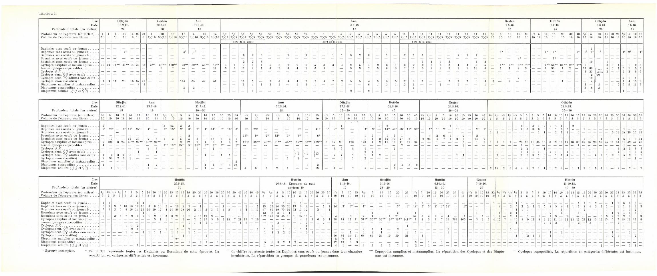
Tableau I

Lac Ottsjön Gesten Ann Ann Gesten Hottön Ottsjön AnnDate 16.2.47. 29.3.46. 31.3.46. 8.5.48. 2.6.46. 2.6.46. 5.6.46. 6.6.46.

Profondeur totale (en mètres) 25 20 18 13 25 45 26 17Profondeur de l’épreuve (en mètres) . . 1 i 5 10 15 20 20 1 10 15 1 1 5 10 15 i/2 t/2 V* i/2 1/2 i/2 t/2 i/2 1-2 1/2 5 5 5 5 5 5 5 5 5 5 h 11 11 ii h 11 11 h h 11 1/2 5 10 15 20 m 5 10 15 20 30 40 1/2 5 10 15 20 25 1/2 5 10 15Volume de l’épreuve (en litres) ........... 10 9 10 10 10 10 9 3X10 3X10 3X10 3X10 3X10 3X10 3X10 2X5 2X5 2X5 2/.5 2X5 2X5 2X5 2X5 2X5 2X5 2tf5 2X5 2X5 2X5 2X5 2X5 2X5 2X5 2X5 2X5 2X5 2X5 2X5 2X5 2X5 2X5 2X5 2X5 2X5 2X5 10 10 10 10 10 10 10 10 10 10 10 10 10 10 10 10 10 10 10 10 10 10

bord de la glace bore de la glace bord de la glace

Daphnies avec oeufs ou jeunes............. 1

Daphnies sans oeufs ou jeunes a........... — — — 1° — — — — — — 3° 1° — — — — — — — — — — — — — — — — — — — — — — — — — — — — — — — — — 1* — — — — — 1* 1* — — 2* 1° 4° 1° — — — 1° 2° — 1°Daphnies sans oeufs ou jeunes b........... — — — — — — — — — — — — — 3 2 3 — — 1 — 3 — — i 1 3 2 3 — 1 — 2 i i — — — 2 2 1 — — — — — — — — — — — — —Bosminas avec oeufs ou jeunes ........... — — — — — — — — — — — — — — — — — — — — — — — — — — — — — — — — — — — — — — — — — — — — — — — 4* — — — — 1* — — — — — — — — - — — — —Bosminas sans oeufs ou jeunes ........... — — — — — — — — — __ — — — — — — 2 2 3 — — — — — — — — — — — — — — — — — i 1 1 3 — — 1 2 — — — — — — — — — — — 10 — 1 — — — — — —Cyclopes nauplius et metanauplius .... 15 12 16** 45** 14 35 8 3** 36** 160** 28** 39** 50** 86** 4 i 7 6 1 5 8 2 2 7 5 8 3 4 2 5 4 2 3 1 3 9 2 3 3 3 4 4 5 5 — \ ** 4** 10** 7** — — \ ** 69** 31** 9** 2** 1 — 1 3 1 1 — 1 2 5Jeunes cyclopes copepodites................... — — — — — — — — 3 7 — — — 53 3 i h 9 1 4 3 4 4 1 6 3 1 — 3 3 7 3 6 8 7 11 5 7 7 3 1 7 10 4 — 1 i 9 3 — — 1 35 1 2 — 36 68 A 5 1 1 6 7 5 5Cyclopes SS............................................... — — — — — — — — — — — — — — — — — — — ' --- — — — — — — — — — — — — — — — --- — — — — — — — — — —- — — — — — — — — — — 4 23 viron 2 — — 2 2 6 3Cyclopes scut. 22 avec oeufs ............... — — — — — — — — — — — — — — — — — — — — — — — — — — — — — — — — — — — — — — — — — — — — — — — — __ — — — — — — — — 2 70 — — — — — — —Cyclopes scut. 22 adultes sans oeufs . . — — — — — — — — — — — — — — — — — — — — — — — — — — — — — — — — — — — — — — — — — — — — — — — 2 — — — — — — — — — 19 — — — 2 1 1 —Cyclopes (non classifiés).......................... i 4 11 20 16 37 27 — — — 144 65 42 26 — — 17 5 — 3 8 4 4 2 7 4 7 2 5 5 4 3 5 5 2 3 i — — 7 5 7 1 5 3 — 4 — 1 — — — — 1 — — — 4 J — — — 1 4 13 6

Diaptomus nauplius et metanauplius . . — — — 8 3 — — 1 4 1 3 1 — 1 3 i — — 1 — — 6 1 2 i 2 1 — — 1 — i — — i — — — 2 — 3 — 1 2 5 8 11 9Diaptomus copepodites ............................ — — — — — — — — — •-- - 3 3 — 1 — — — — — — — — -- - — — — — — — — — — — — — 1 — — — — — — — — — — — — — — — — — — — — 3 8 5 — — — — — — —Diaptomus adultes ( S S et 2?) ........... — — — — — — — — — — 1 — — — — — — 2 — — — — — — — — — - — 2 — 2 — — — — — — — — — — — — — — — — — — — — — — ••• — — — — i — — — i — — —

LacDate

Profondeur totale (en mètres)

Ottsjön12.7.46.

28

Ann13.7.46.

16

Hottön21.7.47.40—50

Ann16.8.46.

18

Ottsjön17.8.46.25—30

Hottön22.8.46.

45

Gesten23.8.46.20—25

Ottsjön24.8.48.25—30

Profondeur de l’épreuve (en mètres) . . 1/2 5 10 15 20 25 10 15 1/2 1/2. 5 5 10 10 15 20 25 35 1l2 1/2 i/2 i/2 1/2 5 10 1 15 1/2 5 10 15 20 25 1/2 5 10 15 20 30 45 1/2 1/2 5 5 10 10 15 15 20 20 i/2 i/2 1/2 1/2 1/2 5 5 5 5 5 10 10 10 10 10 15 15 20 20 20 20 20 30 30 30 30 30Volume de l’épreuve (en litres) ........... 10 10 10 10 10 10 10 10 10 10 10 10 10 10 10 10 10 10 10 10 10 10 10 10 10 10 10 10 10 10 10 10 10 10 10 10 10 10 10 10 10 10 10 10 10 10 10 10 10 5 5 5 O 5 5 5 5 5 5 5 5 5 5 5 5 5 5 5 5 5 5 5 5 5 5 5

Daphnies avec oeufs ou jeunes............. 2 11 65 3 3 1' V ’

1 2 1 1 1 1 3 1 2 1 4 1 2

Daphnies sans oeufs ou jeunes a........... 9° 23° — 2° 11° 27° 4° — 5° 18° 2° 3° 2° 1° 31° 6° 10° 6° 3* 22* — — — 9* — 41* 1° 9° 2° — 1° 2° — 14° 49° 53° 11° 33° — 1° 1° 2° — 1° — — 2° 1° — — — — — 6 3 3 6 3 1 1 5 2 4 — i — — — — — — 1 — — —Daphnies sans oeufs ou jeunes b........... — — — — — — _ — — — — — i i — — — — — — 1 1 — 2 i i — 3 — — — — — 3 12 35 29 13 23Bosminas avec oeufs ou jeunes ........... — — — — — — — — — — 1 2 — — — — — — 13* 9* 2* 12* 5* 1* — 6* — — — — 1 1 — 1 1 1 — — — 4 2 6 1 — 2 — 2 — — — — — — — — — — — — — —- — — — — — — — — — — — — — —Bosminas sans oeufs ou jeunes ........... — 17 — — 11 30 2 8 1 3 5 5 3 — 13 3 3 1 — — — — — 1 4 2 12 70 27 3 — 2 23 4 7 1 2 9 — 14 2 — — — — — — — — — — — — — — — — i — — i — — 4 6 1 5 14Cyclopes nauplius et metanauplius .... 2 102 8 24 30** 22** 109** 94** — — 9 32 9 4 3 1 5 2 19** 38** 49** 51** 45** 32** 36** 229** 1 65 28 120 120 1 2 11 13 11 32 34 — — 1 — — — 3 — 1 3 i i i 1 — 25 25 11 35 15 6 12 15 16 16 38 25 16 20 35 25 11 54 31 42 47 41Jeunes cyclopes copepodites................... 4 — — — — — — — 1°° 18°° igOO 9°° ]0°o goo

6°° 1 OO — JOO — — — — — — — •-- — — — — — — — — — 2 — — — — — — — — 1 — — — — — — — — 1 — 1 — — — — — — — 1 — — — — — — — 1 — — —Cyclopes SS............................................... — — — — — — 5 3 — — 1 — 1 — 1 — — — — — — — — — — — — 3 9 8 4 — — — 1 — — — — — — — — — — — — — — — — — — 1 1 1 — 1 — — — — — — — 1 — — 1 — 6 2 3 3 3Cyclopes scut. 92 avec oeufs ............... — — — — — i — 1 — — — — — ~ — — — — — — — — — 1 1 L — — — 1 2 1 — — — — — — — — — — — — — — 1 — — — — — — 1 1 1 1 — 4 1 — 1 1 — — 1 — — — — 1 1 4 3 2

Cyclopes scut. 22 adultes sans oeufs . . 1 2 3 5 5 8 — — — — — — — 1 — 1 i — — — — — — f 1 f 1 jus — 5 7 7 1 1 2 — — — — — — — — — — 1 1 — — — — 2 — — — 2 3 3 1 6 — 1 i 4 — — 1 — 4 2 1 2 3 5 2 3 2

Cyclopes (non classifiés).......................... 2 39 2 3 i — — — — -- - — — — 1 1 — — 3 i 2 — — — — — — — — — — — . — — — — — — — — — — — — — — — — 1 — — — — — --- — — — 1 — — 1 — 1 —Diaptomus nauplius et metanauplius . . — — — — 5 — — — — — — — — — — — — — — — — — — — — — — — — — — — — — — — — — — — — — — — — — — — — — — — —Diaptomus copepodites ............................ 1 — — — —■ — 4 2 — — — — — 1 1 6 5 22 — — — — — — 1 3 — — — — — — — — 9 4 3 2 — — — — — — — — — — — — — — — — — — — — — — — — — — — — — — — — — — — — —Diaptomus adultes (S S et 2?) ........... — 1 1 — — — 1 — — — — — — 1 — — — — 4 6 3 2 1 — — 13 — 3 — 7 5 — — 1 — — — — — — — — — — — — 2 15 2 3 4 4 2 2 1 1 1 2 2 — 1 1 2 1 1 1 1 — 2 — 2 - 2

LacDate

Profondeur totale (en mètres)Profondeur de l’épreuve (en mètres) . . Volume de l’épreuve (en litres) ...........

Hottön25.8.48.

50

10 10 15 15 20 5 5

20 20 30 30 40 40

Hottön26.8.48. Épreuves de nuit

environ 40

Ann1.10.46.

17

Ottsjön3.10.46.28—29

Hottön6.10.46.45—50

405

1 /2

5t/2

555

55

10

510

5155

155

20

520

5305

305

V?10

510

10

101510

1/2

10510

10

101510

20

102510

1/2

10510

10

101510

20

102510

3510

4410

i/210

510

10

101510

22

10

1/2

5i/2

51/2

51/2

555

55

55

55

10

510

510

510

5155

155

155

155

20

520

520

520

5255

255

355

355

355

355

i i 1 1 i 4 2 1 i i i 1 1 2 i i 3 5 31

134397

3389

2649

3575

20

541952

8

132

12—

2

1 ii

16° 3° 3° — 1° — — — 5° 3° 19° 5° 3° 2° 2° 12° — - 2° — — — — — 4 — 2 51

2

1

2

1i i 5 2 5 4

1i i i 2

24 2 i i

i— i 1

1

8

332

3

— 13 8 3 i 1 — 1 — — — — — — — — — — i — — 2 — 1 — — — — — — — — i — — __ 1 1 2 i — 1 — — — 2 — 1 — — i — — — — i i 2 4 3 3 1

— 162 141 50 45 18 51 15 18 — 1 — — 4 — 5 — 2 4 — 1 21 — 52 6 4 1 4 4 — 1 — — 1 — 1 2 — 2 i — 1 — i — 1 3 — 2 i — — — — 3 3 2 2 2 5 — 310 — — _ — — i 4 2 5 6 3 i 38 15 17 11 31** 25** 36** 16** •>8** 141** 1 4 5 2 7 29 289 460 — 3 1 5 4 12 7 4 10 8 9 h 8 3 10 11 14 18 12 13 21 12 13 13 13 5 7 18 ii 13 8

— — — 2 — — — 1 2 — 1 1 — — — — — — — — — — — — — — — __ — — — — — — — ~ - — — 1 — — — — 1 1 2 — — — 2 — 3 — — 1 — 1 — — — —— — 1 1 1 — — — 1 — — — — — — — — — — — — — 1 — — — — — — — — — — — — — — — — — — — — — — — — — — ■-- - — — — -- - — — — — 1 — — —

1 1 1 — 1 3 i 1 1 — — — — — — — — 2 1 1 — 2 — — — — — — 3 — — — — — — — — — 1 — — — — — — — — — — — — — — — — — — ----- - — — — —

— 1 4 2 2 3 — — 2 1 _ — — — — 1 — 3 2 1 ----- • 4 2 1 — — — — 3 ------ . — — — — — — — — — — 1 — — — — 1 — 1 — — — — — — — — i — — 2 — ------

.--- — — — — — — — — — — 606

392

344

11

1

68 61 24 19 89 21 — 1 — — __— — — — — — — — — — — 1 ----- * 2 i 1 — 1 — — — 1 — — ----- - — — 1 2 1 — — 2 —

— 5 8 3 2 1 2 — — — — — — 12 13 5 3 — — — — — — 3 — 1 — 1 — _ — — — — — — — — — — — — — — — — — — — — — — — — — — — — — — — —

— 1 — — — — — — — — — — — 4 1 — — 4 1 2 1 7 4 2 — 1 — — — _ — — — — — — — — — — — — — — — — — — — — — — — — 1 — — — — 2 i —

Gesten7.10.46.

25

Hottön25.10.48.

40—50

Daphnies avec oeufs ou jeunes.............Daphnies sans oeufs ou jeunes a...........Daphnies sans oeufs ou jeunes b...........Bosminas avec oeufs ou jeunes ...........Bosminas sans oeufs ou jeunes ...........Cyclopes nauplius et metanaupliusJeunes cyclopes copepodites...................Cyclopes SS...............................................Cyclopes scut. 92 avec oeufs ...............Cyclopes scut. Ç2 adultes sans oeufs . .Cyclopes (non classifiés)..........................Diaptomus nauplius et metanauplius . .Diaptomus copepodites ............................Diaptomus adultes (SS et 2?) ........... 1

1 Épreuve incomplète. * Ce chiffre représente toutes les Daphnies ou Bosminas de cette épreuve,répartition en catégories différentes est inconnue.

La Ce chiffre représente toutes les Daphnies sans oeufs ou jeunes dans leur chambre incubatrice. La répartition en groupes de grandeurs est inconnue.

** Copepodes nauplius et metanauplius. La répartition des Cyclopes et des Diapto­mus est inconnue.

Cyclopes copepodites. La répartition en catégories différentes est inconnue.

ö

Fertility of Char (Salmo alpinus L.) in the Faxälven Water System, Sweden

By Alexander Määr

There are no exact data on the char’s fertility nor on development of it and the aim of this short study is to present some illustrative statements on this question. The material at hand is gathered by investigating the distribution area of the char in the Faxälven water system. This distribution area has many advantages for studying the char’s fertility and therefore the problem may be treated from several points of view. These advantages are:

a) the distribution area of the char, which is ca 200 km in length and extends towards SSE, is rich of contrasts as regards the climate and the land­scape (fig. 1) ;

b) the distribution area has a biological barrier and it is in the south;c) the distribution area includes several big lakes with a rich stock of

char. The lakes are situated in a successive order as regards the changes in climate and landscape;

d) no plantings of char from other water systems into this area has been undertaken in a quantity worth mentioning.

Lakes which give material for this research on the char’s fertility, are in­cluded in table 1 together with data on their fundamental qualities. It may be added that the lakes in question are of an oligotrophic type and situated in the mountain landscape on the barrier of the spruce-forest area and reaching in the southern direction the pine-forest plateau, which is typical to the northern parts of Sweden. The material was gathered in these lakes during the years 1945—1948. Egg samples were taken from ripe fish caught during the spawning period on the spawning grounds but only from fish which could not yet be stripped.

After the fish was weighed and measured, the whole ovary was removed, weighed and preserved in 3 per cent formalin. Eggs were counted in labora­tory. All eggs were counted and preserved for each individual separately.

Exact data on the number of eggs of char in Swedish waters, as well as in other countries, are to be found in the literature only regarding a few

59

Table 1. Lakes from which egg samples of char were taken and some oftheir fundamental qualities.

LakeH

eigh

t abo

ve se

a lev

el

in m

Ë

.£a a)Sh M

axim

al de

pth in

mPe

rea fl

uvia

tilis L

.

Coi

tus p

oeci

lopu

s Hec

kel

Lota

lota

(L.)

Phox

inus

phox

inus

(L.)Le

ucisc

us ru

tilus

(L.)Le

ucisc

us idb

arus

(L.)

Esox

luciu

s L.

Salm

o trut

ta L.

Core

gonu

s lava

retu

s L.

Thy m

all u

s thy

mal

lus (L

.)

Petro

myz

on flu

viat

ilis L

.

Leipikvattnet ................. 468.0 5.0 24 +Ankarvattnet ................. 448.0 9.4 72 +Blåsjön............................ 433.5 41.4 152 +Jormsjön ........................ 344.5 35.3 94 +Kvarnbergsvattnet.......... 310.0 67.4 93 + + 1+)Hetögeln ........................ 294.1 22.4 60 + + + + +Ströms Vattudal............. 285.6 147.3 68 + + + 4- + + + + + + +

individuals. In consequence of this one may come to erraneous results, as experience has already shown, when trying to define on basis of incomplete data the fertility variations of char populations in different water systems. Table 2 contains all research materials from the Faxälven water system, i.e. individual number of eggs of 228 specimens and data on 18 specimens from other water systems, which were published by Olofsson (1934).

From the table it is evident that as to the number of eggs and the size of the char two groups of marked difference are to be recognized. These are: the »large char» and the »mountain char», the latter being smaller in size and with more limited number of eggs.

The char in the Faxälven water system belongs to the latter group. As it may be observed, this division is applyable to chars in other water systems. In the lakes of the Faxälven water system, as well as in one particular lake, several char populations of different kind are to be found. They differ in choosing their spawning places and the depth at which they spawn, as well as in spawning time. Table 3 has been constructed to determine the separate populations from the point of their biological difference, and to give a survey on their existence in the lakes in question.

No data are to be found on morphological difference in the appearance of specimens of the populations classified, but groups in one lake may be distinguished from each other by outward observation. But it is an open question in which degree populations in different lakes classified as equal are comparable.

All poulations included in the table are to be found in quite a large amount, depending upon conditions of the lake they inhabit, more precise data are missing only on population V in Lake Jormsjö and Lake Kvarnbergs- vattnet.

Table 2. Egg number in char (Salmo alpinus L.) from various localities, length frequency of the investigated char and length frequency of a larger sample of females taken outside the

fertility investigation.

Water Name ofÖ_o O c/5n Numb e r C f e g g s«5 . 1 , 1 . I .

system lake 'BOhoX! .5g «

i1 1 i i 1 ! 1 1 ! 1 1 1 1 1 i 1 1 j, J,v—1 o JU JU ju JU O O O O o o O : O O o o i ° O O O O O O

Z » CM co CO LO to r- CO OS i 1 CM CM CM CM LOCM co

Leipik-vattnet ii

17 — — — — — — — - —1 2 3

21

14 2

11

21

— 3 3 1 2 2 — — — — —

40 4 2 2 4 6 3 6 7 5 2 2 — i — —

Ankar- — 4 __ — _ _ _ i _ 1 2 _ ___ _ __vattnet — — — i — 1 1 1 — — — —

i 30 — — — 2 2 4 _ 3 4 2 2 4 4 1 i i _— — 1 3 2 2 — 3 2 7 3 2 1 i 2 1

Blåsjön Ii 26 — — — 11

72

31

38

34

21

62

13 2 1 i

— — - — — — — — — —

IV 21 — 1 11 8 11 2 7 2 7 2

fl<u I 62 — 2 13 28 14 2 3> — 1 5 12 20 13 8 2 1 — — — — — — — — — — _ __ _ _ ___ _ __ __ _ _

Jormsjön 100 — 2 12 20 25 23 13 3 1 1 — — — — — — — — — — — — — __ __ _ __ _ _

X — 13 _1 2 — 4

331

15

12

11

—1

— — — —

p3

1 44 — 1 4 7 6 7 2 9 2 1 3 — _ 2 __ __ _ _ __ _ __ _ __ _ _ _ _Kvarn- • —■ — — — — 2 1 6 3 5 6 9 1 4 3 2 1 1 — _ _ _ _ _ _ _ _ _ __bergs- 57 — — — — — 2 2 7 4 11 10 11 3 7 3 2 2 2 — _ 1 — — — _ ___ _ _ _vattnet — 10 — —

2 1 11

21 1 - 1 —

12

1 i 12 1 —

— — —1

——

——

—

Limingen —1

— — —1 —

—— —-

1 ——

——

— —— — — — — — — — —

——

__ _

Hetögeln — 1 — — — - — — — — — — — — — — — — 1 — ~ — — — — - — — —

1111 — . — — — — — 1 1 1 1 2 4 1 — — — — — — _ — — — — _ _ __ _ _

Vattudal 113— — — — — — — — — 2 3 3 3 — — — —— — — — — — 1 3 .9 17 27 22 24 7 1 1 1

Fjällsjö-älv Borgasjön — 1 _

Anger-manälv Gikasjön — 2 — — r— — — — — — — — — — — — — 1 — 1 — — — — — — — —

—

Gardsjön — 2 21

—1 —

— ——

——

—— — — — —

—_ — — —

— — — ~ — — _ _ _

Umeälv < Magasjön — 1 — 11 — — — — — — — — — — — _ — _ _ __ _ _ — _ _ ■ __ _ _ i

■ Storuman — 5 -4— — — _ — — _ — _ _ _ _ _ _ _ _ _ _ _ § _

11

21

21 1 1

Skel- Ilefte-

Södrajaur — 1 —— — — —

— — — — 11

——

——

— —— —

— —-

——

——

— — ——-

älv Bingselet — 2 —— — —

—— —

1 11 —

— ——

—1

—— — —

——

— — — — — —j — _

Luleälv Langas — 4 _ £z 1 — — 1 z 11 z — --

2— — — — z — 1

1— — — ■ — — —

Length in cm 23 24 25 26 27 28 29 30 31 32 33 34 35 36 37 38 39 40 41 42 43 49 50 — 55 57 58 60 614 = Egg number frequency. 4 = Length frequency. 4 = ÇÇ length frequency in experimental catches.

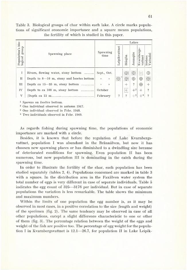
61

Table 3. Biological groups of char within each lake. A circle marks popula­tions of significant economic importance and a square means populations,

the fertility of which is studied in this paper.

Popu

latio

n’s b

io­

logi

cal g

roup

Spawning place Spawningtime

Lakes

Leip

ikva

ttnet

Blå

sjön

Jorm

sjön

Kva

rnbe

rgs­

vattn

etSt

röm

sV

attu

dal

t Rivers, flowing water, stony bottom ........... Sept., Oct. 101 101 EH ©

h Depth to 8—10 m, stony and Isoetes bottom » » i©r 101 © © mhi Depth ca 15—25 m, stony bottom ............. » » + ? © +

IV Depth to ca 100 m, stony bottom ............... October EH # + ?

V (Depth ca 15 m...................................................... February ? ? +3 +4 ?

1 Spawns on Isoëtes bottom.2 One individual observed in autumn 1947.3 One individual observed in Febr. 1948.4 Two individuals observed in Febr. 1949.

As regards fishing during spawning time, the populations of economic importance are marked with a circle.

Besides, it is known that before the regulation of Lake Kvarnbergs- vattnet, population I was abundant in the Brännälven, but now it has choosen new spawning places or has diminished to a dwindling size because of deteriorated conditions for spawning. Even population II has been numerous, but now population III is dominating in the catch during the spawning time.

In order to illustrate the fertility of the char, each population has been studied separately (tables 2, 4). Populations concerned are marked in table 3 with a square. In the distribution area in the Faxälven water system the total number of eggs is very different in case of separate individuals. Table 5 indicates the egg count of 325—3176 per individual. But in case of separate populations the variation is less remarkable. The table shows the minimum and maximum numbers.

Within the limits of one population the egg number is, as it may be observed in most cases, in a positive correlation to the size (length and weight) of the specimen (fig. 2). The same tendency may be observed in case of all other populations, except a slight difference characteristic to one or other of them (fig. 3). The percentage relation between the weight of the eggs and weight of the fish are positive too. The percentage of egg weight for the popula­tion I in Kvarnbergsvattnet is 12.1—26.7, for population II in Lake Leipik-

Table 4. Length, weight and egg data of char from different populationsand lakes.

£

Weight of eggs

Number of eggs£

Weight of eggs

Number of eggs

bß o 'Cß O

£ a -8 5" a .9 s bß .5 G S s~

a .5 Bbß

a;A s O

•-M A03

2 £<ÜX +-> A.bß

*3£

Ö “ j- 2 £apZ

ea) *3?

bßG

a bß "v *3

H

Per

leng

t bßSI

PH £

B

za0) in

g o3 bß lu ÜX £

03h->OH

. bß a; G

bßSh« gPh £

Leipikvattnet Blåsjön

Population II Population II

i 33 335 60 17.9 1519 46 453 i 26 135 35 25.9 648 24 3462 34 350 65 18.5 2143 63 612 2 27 140 30 21.4 595 22 4253 34 415 110 26.5 1865 54 450 3 27 165 35 21.1 603 22 3654 35 370 95 25.6 2242 64 605 4 28 195 35 17.9 612 21 3135 35 370 110 29.7 2532 72 684 5 29 190 40 21.0 717 24 .3776 35 375 90 24.0 1636 46 436 6 29 205 45 21.9 614 21 2997 36 375 95 25.3 2297 63 612 7 29 215 40 18.6 839 28 3908 37 375 85 22.6 2385 64 636 8 29 220 30 13.6 740 25 3369 37 380 90 23.6 1988 53 523 9 29 225 45 20.0 620 21 275

10 37 410 65 15.8 2186 59 533 10 29 235 30 12.7 600 20 25511 37 435 100 22.9 2526 41 580 11 29 240 60 25.0 952 32 39612 38 400 95 23.7 2123 55 530 12 29 250 40 16.0 848 29 33913 38 435 95 21.8 3176 83 730 13 30 215 55 25.5 947 31 44014 38 485 85 17.5 1991 52 410 14 30 250 40 16.0 795 26 31815 39 410 65 15.8 1540 39 375 15 30 255 45 17.6 623 20 24416 39 500 95 19.0 2250 57 450 16 30 265 55 20.7 971 32 36617 40 550 110 20.0 3103 77 564 17 31 315 55 17.4 1125 35 357

18 32 300 50 16.6 807 25 267Blåsjön 19 32 — — — 1075 33 —

Population I 2021

3333

345360

7060

20.216.6

12601074

3832

365298

1 26 150 25 16.6 601 23 400 22 33 365 85 23.2 1105 33 3042 27 175 35 20.0 615 22 351 23 34 415 85 20.4 1109 32 2673 27 180 40 22.2 745 27 413 24 34 425 75 17.6 1167 34 2744 27 190 25 13.1 759 28 399 25 35 430 80 18.6 1144 32 2665 28 200 35 17.5 752 26 376 26 37 465 85 22.9 1152 31 2476 28 — — — 1057 37 —

7 29 195 35 17.9 540 18 276 Blåsjön89

2931

210250

4550

21.420.0

5611144

1936

267369

Population IV

10 31 255 50 19.6 766 24 300 1 23 115 23 20.0 451 19 39211 31 320 60 18.7 947 30 295 2 24 108 22 20.3 410 17 379

12 32 320 65 20.3 1045 32 326 3 24 128 19 14.8 502 20 39213 32 360 85 23.6 1316 41 365 4 25 104 21 20.1 451 18 43314 33 320 70 21.8 993 30 310 5 25 119 18 15.1 507 20 42615 33 330 70 21.2 1020 30 309 6 25 126 18 14.2 325 13 257

16 ’ 33 345 90 26.0 1243 37 360 7 25 134 28 20.8 548 21 40817 33 350 70 20.0 908 27 259 8 25 140 25 17.8 439 17 31318 33 350 80 22.8 1475 44 421 9 25 145 24 16.5 504 20 347

19 33 360 95 26.3 1372 41 381 10 25 150 26 17.3 525 21 35020 33 385 105 27.2 1221 37 317 11 26 150 25 16.6 500 19 33321 34 360 95 26.3 1357 39 376 12 26 169 25 14.7 494 19 29222 34 395 100 27.8 1304 38 330 13 27 135 25 18.5 476 17 35223 34 430 60 13.9 1068 31 248 14 27 137 28 20.4 528 19 38524 35 400 80 20.0 1156 33 289 15 27 142 23 16.1 485 17 34125 35 465 90 19.3 1433 40 308 16 27 155 25 16.1 445 16 28726 36 480 100 20.8 1403 38 292 17 27 160 31 19.3 590 21 36827 37 560 130 23.2 1641 44 293 18 27 161 29 18.0 491 18 30428 38 510 95 18.6 1426 37 279 19 27 170 30 17.6 586 21 34429 38 545 135 24.7 1746 45 320 20 28 140 35 25.0 620 22 44230 39 530 120 22.5 1579 40 297 21 28 160 30 18.7 422 15 263

Table 4. Continued.N

umbe

r

Leng

th in

cm

Wei

ght in

gWeight of

eggsNumber of eggs

Num

ber

Leng

th in

cm

Wei

ght in

g

Weight of eggs

Number of eggs

tlO

.s Rel

atio

n to

wei

ght i

n °/

o

Tota

l

Per 1

cmle

ngth

Per 10

0 gw

eigh

t

'QOÖ R

elat

ion to

wei

ght i

n °/

o

Tota

l

Per 1

cmle

ngth

Per 10

0 gr

wei

ght

50 28 195 35 17.9 601 21 30851 28 200 35 17.5 638 22 319

Population l52 29 185 30 16.2 552 19 298

i 24 110 20 18.1 457 19 415 53 29 185 30 16.2 561 19 3032 25 120 30 25.0 465 18 387 54 29 190 35 18.4 675 23 3553 25 120 30 25.0 467 18 389 55 29 200 30 15.0 707 24 3534 25 135 30 22.5 512 20 379 56 29 210 40 19.0 650 22 3095 25 135 30 22.2 661 26 489 57 29 210 35 16.6 715 24 3406 25 140 25 17.8 380 15 271 58 29 215 45 20.9 549 18 2557 26 125 35 25.9 634 24 469 59 29 260 30 11.5 562 19 2168 26 145 25 17.2 424 16 292 60 30 180 45 25.0 875 29 4869 26 145 30 20.6 517 19 356 61 30 215 40 18.6 627 20 312

10 26 145 30 20.6 526 20 362 62 31 315 55 17.4 803 25 25411 26 145 30 20.6 546 21 37612 26 150 30 20.0 575 22 383 K varn berqsva ttnet13 26 155 30 19.3 468 18 30114 26 155 30 19.3 569 21 367

population i

15 26 160 30 18.7 402 15 251 1 28 185 35 18.1 709 25 38516 26 160 30 18.7 578 22 361 2 28 215 30 13.9 524 18 24317 26 165 30 18.1 487 18 295 3 29 215 35 16.2 636 21 29518 26 170 40 23.5 567 21 333 4 30 210 35 16.6 492 16 23419 27 145 30 20.6 602 22 414 5 30 215 40 18.6 686 22 31920 27 155 35 22.8 550 20 354 6 30 220 40 18.1 666 22 30221 27 155 30 19.3 552 20 356 7 30 230 30 13.0 511 17 22222 27 160 30 18.7 501 18 313 8 30 245 40 16.3 530 17 21623 27 160 25 15.6 532 19 332 9 30 265 40 15.0 660 22 24924 27 160 30 18.7 559 20 349 10 31 245 35 14.2 534 17 21725 27 160 35 21.8 603 22 376 11 31 275 50 18.1 961 31 34926 27 165 30 18.1 381 14 230 12 31 345 45 13.0 684 22 19827 27 165 30 18.1 448 16 271 13 32 255 40 15.6 821 25 32128 27 165 35 21.2 525 19 318 14 32 270 50 18.5 735 22 27229 27 165 30 18.1 600 22 363 15 32 275 35 12.7 665 20 24130 27 170 30 17.6 422 15 248 16 32 275 50 18.1 763 23 27731 27 170 35 20.5 553 20 325 17 32 285 50 17.5 853 26 29932 27 170 35 20.5 568 21 334 18 33 270 65 24.0 814 25 30133 27 170 35 20.5 672 21 395 19 33 295 45 15.2 690 20 23334 27 175 30 17.1 605 22 345 20 33 305 60 19.6 744 22 24235 27 180 30 16.6 460 17 255 21 33 310 50 16.1 860 26 27736 27 180 25 13.8 560 20 311 22 33 310 75 24.1 979 29 31537 27 185 30 16.2 541 20 292 23 33 325 45 13.8 764 23 23538 27 215 35 16.2 617 22 287 24 34 310 60 19.3 856 25 27639 28 155 30 19.3 520 18 335 25 34 330 50 12.1 855 25 25040 28 165 40 24.2 595 21 360 26 34 340 65 19.1 845 24 24841 28 170 35 20.5 587 20 345 27 34 340 70 20.5 1001 29 29442 28 175 40 22.8 828 29 473 28 34 350 70 20.0 1025 30 29243 28 180 30 16.6 445 15 252 29 34 355 60 16.9 1070 31 30144 28 180 40 22.2 673 24 373 30 34 370 80 21.6 1111 32 30045 28 185 35 18.9 495 17 267 31 34 390 80 20.5 1026 30 26346 28 185 35 18.9 583 20 315 32 34 405 60 14.8 1049 30 25947 28 185 40 21.6 660 23 356 33 35 355 65 18.3 1124 32 31648 28 190 30 15.7 492 17 258 34 36 390 55 14.1 717 19 18349 28 190 35 18.4 592 21 311 35 36 390 80 20.5 1307 36 335

Table 4. Continued.

g

Weight of eggs

Number of eggss

Weight of eggs

Number of eggs

y bß y bß .©

& _G 3 o 2 bß _G B3 ® s bß

G -S G —<

33z

bßGyJ W

eigh

t

in g

.2d bß

"y yos » To

tal

Per 1

i

leng

thPe

r 10'

wei

ght rQ

2Gz

bßGy

bß‘y£ in

g

O

B 5'"3 y A To

tal

Per 1

i

leng

thPe

r 101

wei

ght

36 36 395 70 17.7 1087 30 275 Ströms Vattudal3738

3637

430430

11570

26.716.2

13591073

3726

316249

Population II

39 37 445 90 20.2 1385 37 311 1 32 280 75 26.7 1338 41 47740 37 495 110 22.2 1645 44 332 2 32 315 70 22.2 1369 42 43441 38 420 65 15.4 1046 27 249 3 33 220 60 27.2 1067 32 48542 38 425 80 18.8 1001 26 235 4 33 230 60 26.7 911 27 39643 39 520 90 17.3 1242 31 238 5 33 310 80 25.8 1368 41 44144 40 590 130 22.0 1657 41 280 6 34 320 70 21.8 1120 32 350

7 34 345 70 20.2 1215 35 3528 34 320 80 25.0 1382 40 4309 35 320 85 26.5 1231 35 384

10 35 350 60 17.1 1407 40 40211 35 365 50 13.6 890 25 243

vattnet 15.8—25.6 and population IV in Lake Blåsjö 14.2—-25.0. It is worth mentioning that in spite of the size of the fish this percentage relation is varying within all populations between 12 and 27. It is needless to discuss this fact more closely, for the preserved eggs have been weighed in different stages of development and results of weighing may be unequal.

It is known that egg number of different populations is varying in a certain degree (table 2) and that the variation limits concerning the popula­tion are different.

The average of the total number of eggs characterizes the difference be­tween separate populations (table 5 indicates the average number). This average is not occasional, but identical to the real average of population in the lake concerned. This can be stated by equality of the average size of fish (weight and length) and by that of the spawning ?? fish population, the latter being calculated on basis of material secured by an experimental catch. The table does not contain data on Lake Blåsjö, for there was no material at hand from spawning places there. But experiments for marking of the char in the lake in the year 1946 show that several populations are to be found in the same place and therefore materials got by experimental catches from places where fish are not spawning, are not used.

The average of the total egg number as regards the separate populations is varying in proportion to the average size of the fish (fig. 4), i.e. the average number of eggs of different populations has a certain relation to the average length and weight of the population. In general, it may be stated that the average of the number of eggs of the populations studied shows,

65

1700 -

• Population I1600 -

o Population II1500 -

+ Population IV1400 -

1300 -1200 -

1100 -

s. looo -900-

u 800 -

700 -

600 -

500 -

400

23 24 25 26 27 28 29 30 31 32 33 34 35 36 37 38 39length in cm

Fig. 2. Relation between total length and number of eggs of the char populations inLake Blåsjö.

concerning the size of the fish, the same relation which is typical for fish of one population.

Of the populations studied the Blåsjö population IV has a minimum number of eggs — the average being 490 eggs per fish. The Leipikvattnet population II has a maximum number — 2206 per fish. It indicates that difference in fertility may be fourfold. When comparing the number of eggs of populations in one lake where it is possible — on basis of data from Lake Blåsjö (tables 4, 5) — the result is that even in this respect the difference may be quite a large one, ca threefold. The average number of eggs of population I in Blåsjö is 1106 per fish; population II 875 and population IV 490 eggs per fish. Fig. 2 indicates the difference between these 3 populations concerning the number of eggs and classes of length.

This shows that the total of eggs in one population is depending on average size of the fish belonging to this population.

It is generally known that the average of the total number of eggs of5

66

2300-

2200-

2100 - r600

2000-

1900-

1800-

1700-

1500-

o 1300 -400 ^

■2 1200-

1100-

o 1000-

900- -300

800-

700-

600-

500- -200

23 24 25 26 27 28 29 30 31 32 33 34 35 36 37 38 39 40Length in cm

Fig. 3. Regression lines for total length and total fertility (---- O------) as well as relativefertility (— • —) in char.

separate fish populations belonging to the same systematical unit but dwelling in different waters, is varying in a certain degree. Naturally the same pheno­menon may be observed with char populations in the Faxälven water system. But in this case the problem is more complicated, for populations of several units are represented. Therefore it is impossible to answer the question, if the number of eggs of populations concerned is varying in the limits of one systematical unit or in the limits of populations belonging to different systematical units, and it is difficult to state the development of total fertility of populations in relation to the factors of the environment.

Discussing the populations in the Faxälven water system regardless to the

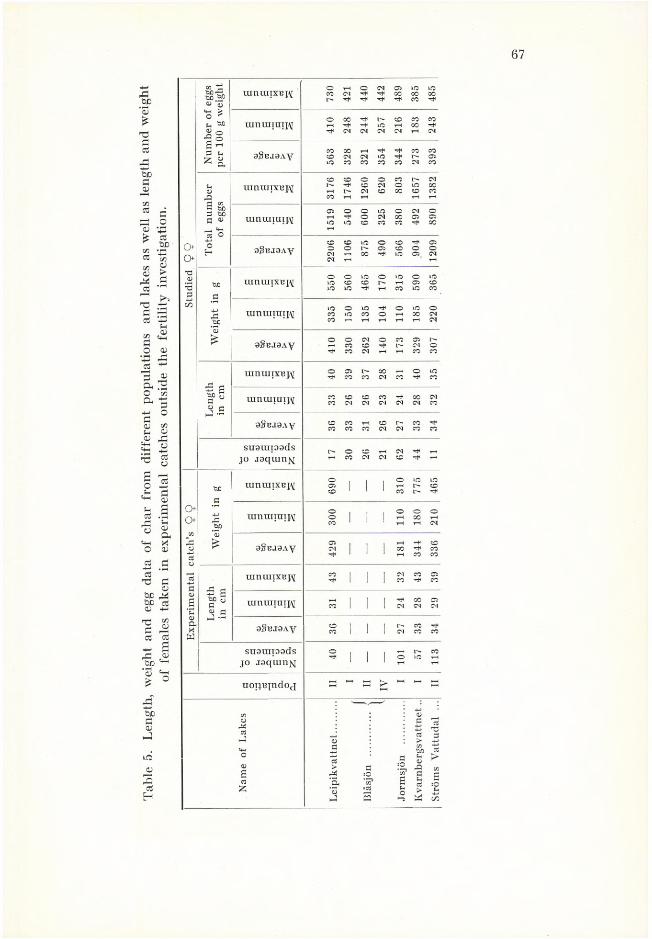
67

ac<v*

TJfifi

ti/Dfi

0)£

fiO

fi Ö0 •

0)

aTJfifi

0)►.5

<Drfi

a :sO c/3

”fi•M Ofiq_> c/3

?h 03 <D

J+H O «+h 4L^ u

OÎH

f-CfirfiO a;

aXaj

-2 .5fi ,,H T5 fi

03£/D ^ fcß fi <13 -M

T5 fi fi fi

03

rfi ^Ö0 ^'S ^ £ °

£”Sbc<03

Hfi

kfi0)3fih

Stud

ied Q

9N

umbe

r of e

ggs

per 1

00 g

wei

ght

umimxBjv 730

421

440

442

489

385

485

innuimij\[ 410

248

244

257

216

183

243

oSejsay

563

328

321

354

344

273

393

Tota

l num

ber

of eg

gs

uinmiXBj\[

3176

1746

1260 62

080

316

5713

82

mnmiuij

1519 54

060

032

5

380

492

890

oSBjaAy

2206

1106 87

549

0

566

904

1209

Wei

ght in

g ranmixnj\[ 550

560

465

170

315

590

365

ummiuij\[ 335

150

135

104

110

185

220

OgBJOAy

410

330

262

140

173

329

307

Leng

th

in cm

mnmixnjv 40 39 37 28 31 40 35

uinuiiuipv 33 26 26 23 24 28 32agBJOAy 36 33 31 26 27 33 34

susrapads jo joqumj^

t" O to 1—1 CM ^ rHt—l CO <M CD ^ T—1

Expe

rimen

tal ca

tch’

s 9 9

Wei

ght in

g tunuiiXBjv 690

310

775

465

ranunuij^ 300

110

180

210

agBJOAy

429

181

344

336

Leng

th

in cm

uinraixnpv 43 32 43 39

umuimijv r—i i i I oo csCO 1 1 1 <M <M CM

ogBjaAy 36 27 33 34

suarapads jo jaquin^

40 101 57 113

uoijnjndoj ~ ~ a > " 1-1 a

Nam

e of L

akes

Leip

ikva

ttnet

......

......

...

Blå

sjön

...........

......

.... J

Jor m

sjön

.............

......

..

Kva

rnbe

rgsv

attn

et..

Strö

ms V

attu

dal ...

68

systematical units, we see that char, as regards the number of eggs, are dispersed so that populations producing a larger number of eggs are dwelling in the edges of the distribution area — in the Leipikvattnet and Ströms Vattudal, which are the outer lakes of the water system (fig. 3).

As to different populations, for instance in Blåsjö, the number of their eggs is degrading in relation to the depth of spawning places and delay of spawning time.

It may be added that char populations with limited number of eggs are to be found in central parts of the Faxälven water system.

More important is the problem of relative fertility. With relative fertility number of eggs per 100 g of fish weight is indicated, whereas total fertility means absolute number of eggs per fish. It is known, that the relation between

69

total number of eggs and fish length is a positive one, and that every population has its own typical regression line (figs. 2, 3). There is a relation between rela­tive fertility and fish length too, but it is a negative one, as is evident from fig. 2, which shows the corresponding regression lines for certain populations. It may be mentioned that relative fertility of populations I, II and IV in Blåsjö and that of population I in Jormsjö does not show any statistical differences. As to fish in other lakes, it seems that the number of individuals studied from population I in Kvarnbergsvattnet and population II in Ströms Vattudal is too limited to draw final statistical regression lines for them. But the regression lines at hand indicate that the relation between number of eggs and fish length is, analogically to other populations, a negative one too. It is very interesting that individuals belonging to populations in Leipikvattnet and Ströms Vattudal, are of larger size and have a higher relative fertility than that of other populations. It is apparent that the difference between relative fertility of various populations is due to genetic factors, as theoretical chances for similar modification are very few. It is difficult to find out a modification factor common for populations in Leipikvattnet and Ströms Vattudal, as well as for other populations, the physical conditions in the lakes mentioned being extremely different.

If trying to systematize the populations as regards their relative fertility, following main groups may be recognized:

1) Low relative fertility: Blåsjö populations I, II and IV (Blåsjö popula­tion I shows somewhat higher fertility) ; Jormsjö population I and Kvarn­bergsvattnet population I;

2) high relative fertility: Ströms Vattudal population II;3) highest relative fertility: Leipikvattnet population II.An attempt was made to classify different populations into groups (table 3)

according to their biological differences in the whole distribution area, as well as in separate lakes. Comparing the graduation of relative fertility of different populations, it is evident that graduations of relative fertility do not follow the biological division into groups, for instance, the biological type of char indicated as population II is to be met with in all groups of relative fertility.

Relative fertility, as we could see in case of total fertility, evidently follows the geographical gradient and therefore differences in fertility show a geo­graphical trend. Populations in the central parts of the distribution area have lower fertility, whereas fertility of populations in border regions of the distribution area is higher. Char in Leipikvattnet and Ströms Vattudal inhabits the edges of the distribution area (concerning lakes investigated). Even the remarkable size of fish belonging to these populations indicates it. The size of fish depends upon that these lakes are thinly populated, as it is common in extreme regions of the distribution area.

Total fertility, depending upon size of the fish, is higher too in extreme

70

regions, being relatively higher on account of a higher relative fertility. But it is already known that size of fish normally does not cause a high relative fertility, as we may notice in the case of populations in Leipikvattnet and Ströms Vattudal, for there is a negative relation between the relative number of eggs and the size of the fish. This indicates and sharply marks differences in fertility.

Owing to research in the lakes of the Faxälven water system, it may be assumed that fertility differences of populations are due to genetic selection, as mentioned above. If so, it would be easy to explain (see a paper by Svärd­son in this report) the differences between the separate groups of relative fertility. Svärdson assumes that the natural selection of egg number on the limits of one species’ area may have the consequence that in populations with weak intraspecific competition the number of eggs should increase. On the contrary, the number of eggs should decrease in the populations with a strong intraspecific competition and there the size of eggs is on the contrary favoured by selection.

Increasing egg number of char populations in the lakes situated lower or higher in the Faxälven water system thus seems dependant upon thin popula­tions, and main losses are not due to intraspecific competition, but to factors of the environment or to competing power of other fish. Consequently, in this case inter- or extraspecific tension exceeds the intraspecific one. In the central lakes of the Faxälven water system the situation is a contrary one. There the more favourable environmental factors involve sharpening of intraspecific competition and consequently the egg number is decreasing.

References

Olofsson, O. 1934. Rommängd och romsvällning hos rödingen. Svensk Fiskeritid- skrift 43: 277—279.

Experiments in Lake Väner on the Influence on Fish ofBomb-Dropping

By Carl Puke

In Lake Väner, the largest lake in Sweden, with a surface of 5,550 km“ there occurs, in addition to many other valuable fish, a large stock of pike- perch (Lucioperca sandra Cuv.), which is the object of profitable fishing. For spawning the pike-perch use certain larger bays in the lake. One of them is the so-called Lake Detter in the southern part of the lake with a surface of about 30 km2 and with an average depth of 2 m. In and close to this bay the Swedish Air Force has dropped bombs during training. This is thought by the fishermen to have severely damaged the fish, especially the pike-perch and their spawning. Investigations were therefore made during 1946 and 1947 by a committee appointed by the Swedish Air Force after an appeal by Svenska Insjöfiskarenas Centralförbund (Swedish Federation of Lake Fisherman) at the suggestion of Kungl. Lantbruksstyrelsens Fiskeribyrå (the Fishery Office of the Royal Swedish Board of Agriculture). The present writer was asked to draw up a plan for the experiments and carry out them in collaboration with the committee.

Bombs of various types and with different charges were used.1 The bombs were dropped from an aeroplane or placed by hand on or close to the bottom of the lake and blown up electrically. During the experiments the bottom depths and bottom conditions were changed. Varying quantities of fish 2 were put into rather large steelwire cages, placed in a straight line on the bottom of the lake at different distances up to 100 m from the spot selected for the explosion. 5—6 cages were used every time. Both large and small fishes were used.3

1 Training bomb = cement-container with little black powder-charge12 kg shell bomb=thick-walled bomb with 1 kg trotyl charge 50 kg mine bomb = thin-walled bomb with 28 kg nitrolite charge

250 kg mine bomb = thin-walled bomb with 105 kg nitrolite charge explosive charge for bombs placed by hand with 0.5 kg trotyl.

2 Chiefly Abramis brama L., A. blicca Block, A. faraneus L., Leuciscus erythropthal- mus L., L. rutilas L., Lucioperca sandra Cuv.

3 Large fish = fish with a weight of 200—1,000 g or more; small fish = fish with aweight of 5—10 g.

72

The bursting of a 50 kg minebomb on a clay bottom mixed with sand and with a water-depth of 1 m.

The results of the experiments proved that the training-bombs did practic­ally no harm. Only if one was actually placed in a cage and detonated, were the fish rendered unconscious for a short time, about ten minutes. After dropping a large number of bombs from a plane, no unconscious or dead fish could be observed in the area concerned.

The effect of charged bombs was quite different. A twelwe kg bomb (1 experiment) on a sandy bottom mixed up with clay, certainly killed no large fish within a distance of 5 m of the bomb, but they were rendered unconscious about 20 m from the bomb site. Half of the small fish were dead and the rest unconscious within a distance of 10 m. The stupefying effect was perhaps noticeable at a distance of 15 m. At a distance of 25 m there was no effect at all.

The explosion of a 50 kg bomb (3 experiments) rendered large fish unconscious at a distance of 35 m and killed them at a distance of 15 m. Small fish died at a distance of 15 m and became unconscious even at a distance of 30 m. But at a distance of 40 m both the large and the small fish was undamaged.

Using a 12 kg explosive bomb (1 experiment) at a depth of 1 m on a hard, rocky bottom, the reaction was considerably greater than on a soft bottom. In this case all the fish within a distance of 10 m were dead and within 25 m unconscious. At 40 m distance — unexpectedly enough — nearly all were dead, only 1 lived and was not even unconscious.

Two experiments were made with charged bombs dropped from a plane. The depth of the water was greater, 2 to 4 m. The difficulty of dropping

73

bombs in the area containing the experiment-cages resulted in the explosions not taking place as near to the cages as was desirable. In the first experiment, a 50 kg bomb caused no damage in 2 cages only 50 m from the spot. In the second experiment, when a 250 kg bomb was employed, the fish became unconscious in the cages 30 m away, but no fish were killed. Symptoms of unconsciousness were found even at a distance of 70 m. At a distance of 90 m no influence could be observed.

On the explosion of charged bombs, a number of fishes always emerged round the goals. Most of these were small. The area was, nevertheless, rather limited and did not extend farther than the area in which the fishes in the cages were rendered unconscious. The number was estimated at about 200— 400 fish, when the 50 kg bombs were exploded.

In order to study the after-effects the cages were controlled in 2 special experiments with both large and small fishes, not only immediately after the explosion but also some time after. 50 kg mine bombs were employed. Un­conscious fish proved to recover completely after 24 hours and after a further 24 hours all fish were in good condition, as also the fish which did not appear to have been harmed by the explosion.

Thus, only the charged bombs caused direct damage. In no case did the influence go beyond a distance of 80—90 m from the explosion. Using small or medium bombs (12 and 15 kg) the distance was only 20—40 m. No fish were killed at a distance of more than 50 m from the explosion. Softer bottoms had a damping influence on the explosive effect, as did also the depth of the water. Larger charges caused greater damage. Larger fish had much greater resistance than small ones, which were killed at a distance 2—5 times greater than that at which larger fish were killed (table 1).

Table 1. Comparison between the distances from the explosion at which large and small fish were killed by the bursting of bombs.

Distance in m from the bomb to Fish species the experimental eages

12 kg bomb 50 kg bombSmall fish ........................................ 10 25Large fish ........................................ 1—2 10

Apparently death was chiefly caused by damage to the blood-vessel-system and of the swim-bladder. Heart and dorsal-aorta had often been completely burst in the specimens killed. The unconscious fish showed balance dis­turbances, lying on their sides, and reduced breathing movements. Those symptoms disappeared after a time and the fish swam down again after having drifted on the surface.

The effect of a single bomb or of some other such explosion in the water does not seem to be very great. Repeated explosions on the same spot can

74

have an influence even beyond the area effected by the actual explosion. After an explosion new fish gradually fill up the area and get killed by a repeated explosion. In this way the damage can be great indirectly, especially if the explosions occur at suitable intervals.

Experiments elsewhere have also proved the direct damage not to be so extensive. Dahr (1946) for example, states that the firing off of 750 kg novit had a killing effect at a distance of 100 m, but not at a distance of 300 m. Further, he asserts that firing off of 2250 kg novite only rendered the fish unconscious at a distance of 300 m. Schiemenz (1943) also states that the effect does not extend very far even with large charges. Eklund (1946), Fitch and Young (1948) and Gennerich (1932) have arrived at similar results.

References

Dahr, E. 1946. Några rön angående undervattenssprängningars inverkan på fisk­beståndet. Svensk Fiskeriticlskrift 55: 42—45.

Eklund, C. R. 1946. Effect of high explosive bombing on fish. Journ. Wildlife Management. 10: 72.

Fitch, J. E. and Young, P. H. 1948. Use and Effect of Explosives in California Coastal Waters: 53—70.

Gennerich, 1932. Die Wirkung von Sprengungen auf den Fischbestand in stehenden und fliessenden Gewässer.. Zeitschrift f. Fischerei. 30: 261—268.

Schiemenz, Fr. 1943. Fischfang durch Sprengung. Fischereizeitung 46: 83—85.

r

A New Water Sampler

By Carl Puke

For investigations of shallow and especially bottom water I have con­structed a water sampler differing from the prevailing types. The older samplers of the SpiTTA-lMHOFF-type are based on a flowing-through of water for such a time that the water in the sampler can not possibly be influenced by the air, which the apparatus holds in the beginning. Against that Brönstedt’s, Buttner’s and Friedinger’s apparatuses allow water to run through the cylindrical sampler without restraint, while the sampler is sinking down. The sampler constructed by the present writer chiefly consists of a piston, that sucks up the water in a cylinder.

Figure 1 shows the construction. In the cylinder (a) runs a piston (b), that is fastened to the piston-rod (c). The piston-rod is moved by a frame (d) soldered on the cylinder. The cylinder is suitably made of a brass tube with a two mm thick wall. Before taking the samples the piston-rod is pushed down, in such a way that the under edge of the piston reaches a bit farther than the under edge of the cylinder, as the figure shows. So the elastic turns stretched (e). A pawl (f) prevents the piston coming up again. The pawl is kept on its place by the stretching, while the sampler is sinking down to the desired depth. A lead releases the pawl. Then the piston led up and the cylinder is closed by a closing-stopper (h) fastend below on the piston- rod and connected with a taperane (i). The temperature can be read off on the thermometer (k).

Certain special arrangements can be fixed to the apparatus, if desired. If a glass-cylinder is used, the thermometer can be placed between the closing- stopper and the piston. In that case the glass-cylinder can be fastened to the frame with an elastic, that embraces the upper edge of the cylinder. The part of the piston-rod that the closing-stopper is fixed to, can be reduced (according to figure 3) by dividing in several parts, which run one in another. The distance between the closing-stopper and the cylinder can be shortened, which is convenient when studying the bottom conditions. In such a case a supporting frame must be fixed to the cylinder. On that frame the closing-stopper can rest.

76

.. .(b)

Figure 1: Water-sampler. Figure 2: Lead and pawl. Figure 3: Parts of piston-rod, which run one in another.

The size of the above described water-sampler can be chosen completely according to the demand. For certain investigations I have made a type with a capacity of 100 cm3, that has operated excellently during the taking of some hundreds of samples.

Bottom Fauna and Environmental Conditions in the Littoral Region of Lakes

By Carl Puke

(Preliminary report)

Attention was especially directed to the importance of the littoral fauna of lakes by Wesenberg-Lund’s (1909) fundamental work. He laid open the difference between the fauna in the surf zone, particularly at an exposed locality and the fauna in the vegetation. In spite of that the littoral fauna has not been the object of such a comprehensive study as the profundal one. The cause of that may chiefly have been the want of methods of quantitative determination. Nevertheless results can be found in connection with profun­dal investigations. Thus Wundsch (1919) has made more systematic studies on the fauna of the shore. But only when BzoSKA (1931, 1936) had con­structed a drill on the basis of Lang’s bottom sampler, was it possible to make more careful quantitative investigations in the littoral zone, especially of the parts with vegetation.

By means of such a drill I have made investigations in Lake Malar and in some lakes in the surroundings of Stockholm. For comparing the lakes one with another it has proved necessary to transfer the studies to a shore not too exposed to the winds and with organogen bottom. According to that, such places were selected and biological as well as hydrographical samples have been taken at certain stations in profiles from land to the free water. The number of stations varied, but always lay so that representative samples were received of the Phragmites-belt covering inner-, middle- and outermost part of it, also, of the Nymphaeaceae-belt and of the submerse vegetation region as well as of the bottom without vegetation. At every station 2—3 samples were taken with the drill. The samples were preserved and then examined in the laboratory. Taking of-water samples and measuring of tem­perature always took place immediately before the mentioned investigations. Determinations were made of the oxygen and pH content and in Lake Malar, besides that, amongst other things, of carbonic acid content.

78

Table 1 a. Total average number of animals per m3 in the littoral zone at the bottom of Lake Mälar, collected during different periods in various zones.

Zone July 1940 October 1940 February 1941 May 1941Phragmites-beXt, middle .................. 10,450 2,800 drained 2,575Nymphaeaceae-belt .......................... 965 2,375 2,100 1,175Cladophora-belt ................................ 700 2,650 2,600 2,275

Table 1 b. The percentage of Asellus aquaticus of the whole bottom fauna in the littoral zone of Lake Malar during different periods and in various

zones.Zone July 1940 October 1940 February 1941 May 1941

Phrcigmites-belt, middle...................... 9 44 drained 41Nymphaeaceae-belt .............................. 2 3 7 3Claclophora-belt .................................... 40 48 68 58

Table 1 c. The percentage of Chironomids of the whole bottom fauna in the littoral zone of Lake Malar during different periods and in various zones.

Zone July 1940 October 19401 February 1941 May 1941Phragmites-beXt .................................... 57 3 drained 5Nymphaeaceae-belt .............................. 54 78 60 60Ctadophora-belt .................................... 25 18 10 12

The results found up to now, show changing conditions during the course of the year. Thus the Phrag mit es-belt in Lake Malar sheltered a very rich fauna during the summer with up to 10,000 individuals per m2, while in wintertime only a third of that quantity was found in that zone. In the winter Asellus aquaticus and Chironomids were predominant. In the Nym- phaeaceae-belt the latter doubtless were the most important, while Asellus here was of subordinate importance. Asellus returned in quantities in the submerse Cladophora vegetation. The other components of the fauna were always comparatively few in number, although those at certain times could be rather common. Table 1 furnishes information about the results offered here. In the course of the year the chemical investigations outside the Phrag­mites-helt showed only a small variation of the water conditions. High oxy-

Table 2. Oxygen content in mgl, carbonic acid in mgl, temperature (in |°C) and pH values at the bottom in the littoral zone of Lake Malar.

0) 27.6.1940 14.10.1940 31.3.1941 20.5.1941oN o2 co2 tp PH o2 C02 tp pH 02 C02 tp pH o2 co2 tp pH

t 1.96 20.4 19.8 6.6 8.16 9.1 10.2 7.0 0.36 30.2 0.3 6.4 8.98 11.5 7.6 7.6it 8.84 2.3 18.3 7.8 9.79 5.8 9.6 7.3 8.72 10.9 0.7 7.0 14.02 1.2 7.7 8.6

hi 9.63 1.5 17.9 7.8 9.38 5.2 9.5 7.3 12.22 4.6 1.2 7.5 13.65 0.0 7.4 8.1

Zone I = Phragmites-heXX. Zone ll = Nymphaeaceae-Xie\t. Zone III = Cladophora-heXt.

79

Fig. 1. Oxygen content in mgl and pH at the bottom in the littoral zone in some lakes near Stockholm. Stat. 1 = inner zone of Phragmites stat. 3 = middle zone of Phragmites,

stat. SÿsNymphaeaçeae-belt, stat. 7 = bottom without vegetation outside theNymphaeaceae-belt.

gen content and high pH value dominated as a rule, while carbonic acid supply was small. In the Phragmites-belt these values were high only in the circulation periods in spring and autumn, especially in spring. In summer and winter the oxygen, and hydrogen concentration declined and carbonic acid increased instead (table 2).

These conditions were mostly the same in the littoral region of the rest of the other investigated lakes too. The chemical investigations in those lakes

80

have only included the determination of oxygen and hydrogen in content. The diagram, figure 1, shows the marked sinking of oxygen in the lower parts of the profiles during the summer, while conversely the oxygen content was high in spring and autumn. Even in winter the oxygen was low there. The pH values too are low in the inner parts, while the values in the outward parts are high. In summer and winter the values lie below the neutral point in the inner part of the Phragmites-belt, while the values especially in spring can rise over that point.

The whole gathered faunistic material has not yet been examined, but the results found up till now generally confirm the results of Lake Malar. The most important components of the fauna are Chironomids, Asellus aquaticus and Oligochaeta. The Chironomids appear to fill a larger place than in Lake Malar, while the number of Asellus seems to be smaller. In Lake Malmsjö the total number of individuals in the midde of the Phragmites-belt increased for instance to about 10,000 per m2 during the month of July, while the same number was 2,400 per m2 in the winter samples, comparative with the values of Lake Malar. From 6 lakes I got the following total number of individuals per m2 by samples from the middle of the Phragmites-belt in spring: 6,500, 6,000, 4,350, 3,200, 2,700 and 2,100. The samples cannot be directly compared, but in any case they give an idea of the supply of bottom animals in littoral type in those lakes. More figures could be quoted but shall suitably be deferred until later papers.

References

Rzoska, J. 1931. Bemerkungen über die quantitativen Erfassung der Litoralfauna. Verh. d. Int. Ver. f. theoret. u. angew. Limnologie 5: 261—269.

— 1936. Über die Ökologie der Bodenfauna im Seenlitoral. Arch, d’Hydrobiologie et d’Ichtyologie. 10: 76—171.

Wesenbekg-Lund, G. 1909. Die litoralen Tiergesellschaften unserer grösseren Seen.Int. Revue cl. ges. Hydrobiologi 1:574—609.

Wundsch, H. H. 1919. Studien über die Entwicklung der Ufer- und Bodenfauna. Zeitsclir. f. Fischerei 20: 408—542.

Environment and Productivity of Lakes near Stockholm

By Carl Puke

(Preliminary Report)

To demonstrate the productivity of our lakes it appears necessary to make intensive studies on the environment and production in limited zones. Only then is it possible to get a clear conception of the series of complicated causes which have to be considered. To this end, I have studied the lakes near Stockholm for many years.

The territory investigation comprises both the whole peninsula Södertörn, and the north-eastern quarter of map-sheet 75 Stockholm, excluding Lake Malar. It includes rather a large number of lakes. Larger ones are for in­stance the lakes Vallentunasjö and Drevviken. Only four lakes are larger than 400 har; ten larger than 200 har, and more than fiftysix have an extent of 25 har. Further, many small waters exist, some of which must be called ponds.

The deepest lakes were thought to lie in the strongly folded territory of Södertörn, a principle relation, which Lundquist (1930) has already demonstrated. This turned out to be correct. The deepest may be Lake Flaten in the Tyresö district (25 m) and Lake Albysjö of Fittja. Otherwise the number of lakes with a depth of more than 10 m is very small. Most of the waters in Södertörn generally have a depth of between 4 and 8 m. North of Stockholm the lakes are usually shallow, due to the flat country. The large Lake Vallentunasjö is only 5.7 m deep.

The summer temperature in the epilimnion rises as a rule to between 20 and 22 L. In hot summers, however, as in the year 1945, considerably higher temperatures were recorded. The temperature of the surface water in Lake Källtorpssjö was then 28.5° C. The bottom temperatures in the lakes with hypolimnion generally lie between 10—15u C. The ice-covering usually occurs in the middle of December and the ice melts at the beginning of April.

The oxygen supply is, as a rule, good throughout the year in the higher lakes with clear water, as for example in Lake Ålsjö. In the deeper

6

82

Table 1. Oxygen content and temperature at the bottom of certain typicallakes near Stockholm.

Vallentunasjön Drevviken Ålsjön

ht. above sea-level... 7 19 52area liar ......................... 612 568 30date .................................... 31.7.1947 11.3.1947 31.6.1947 21.3.1947 27.7.1945 20.3.1946depth m.............................. 4 5 9 10 8 7.502 mgl .............................. 7.3 0.61 1.22 4.54 5.14 6.9802 °/o.................................... 78.6 4.6 11.0 34.0 47.2 52.9tp + °C .............................. 20.6 3.8 11.7 3.6 12.4 4.1

(ice) (ice) (ice)

Table 2. Environmental conditions in the surface water of certain typicallakes near Stockholm.

Vallentuna­sjön Drevviken Källtorps-

sjönÅlsjön

lit. above sea-level .................................... 7 19 23 52date ......................................................................... 31.7.1947 31.7.1947 31.7.1947 1.8.1947H . 18° . 10-6 .................................................... 237 133 77 22electrolyte content mgl ......................... 178 100 58 17total hardness German grades ......... 6.2 3.5 1.2 0.3carbonic content mgl ............................... 105 47 13 4.5PH ......................................................................... 8.7 7.7 7.3 6.7

lakes on a lower level surrounded by built up areas, the oxygen content in the hypolimnion is lower in summer and winter. In certain polluted lakes hydrogen sulphide appears, for instance in Lake Järlasjö. In summertime the oxygen content is high troughout the shallow lakes. But in the hot sum­mers, as in the year 1945, when strongly marked waterlayers were formed, the oxygen contents remained low even in the shallow lakes. At the bottom of the only 4.5 m deep Lake Ältasjö the oxygen content was only 0.46 mgl, corresponding to a saturation of 4.9 '%. The temperature was 19.9° C. at the same time. The shallow lakes become poor in or without oxygen in the winter. This occurs even in such large lakes as Lake Vallentunasjö (see table 1).

The hydrogen ion concentration is closely connected with the height of the lake surfaces above sea-level. The high-situated lakes of the central plateau of Södertörn are acid, abounding in humus. As a rule, lower-lying lakes are alkaline at least in the epilimnion.

To ascertain the amounts of electrolytes a determination of the con­ductivity was made. Low-lying lakes with a rich contribution of nutriment from their surroundings are rich in electrolytes, in the high-lying lakes the situation is just the reverse (see fig. 1). The total hardness and Ihe carbonate content were also determined. These values follow those for the electrolytes (see table 2).

83

mabovesealevel

Fig. 1. The relations between the height of the surfaces above sea-level and the electrolytic conductivity in the surface waters of 30 lakes near Stockholm.

In the bottom fauna of the low-lying lakes Oligochaeta and Chironomids dominate, for example those belonging to the plumosus and bathophilus groups. Moreover, in winter large quantities of Saiomyia are found, par­ticularly at the bottom of the large lakes in the valley of the river Tyreså in Södertörn, for instance in Lake Magelungen. Larvae of the bathophilus group have been found in varying numbers and together with large quan­tities of small Orthocladiines even in water poor in electrolytes.

The plankton flora is numerous in the low-lying lakes. The distribution of the various species agrees well with Teiling’s (1916) earlier investigations. Cyanophyceae are frequently found especially in the electrolytic lakes north of Stockholm. The Microcystis, Anabaena and Oscillatoria species form waterbloom. In the lakes of Södertörn, Ceratium hirundinella and Tabellaria fenestrata seem, to be at least equally common. Thus Ceratium hirundinella forms waterbloom in Lake Drevviken. The high-lying lakes are poor in phytoplankton, and that which occurs is generally Desmidiaceae.

84

The zooplankton includes in summer particularly Daphnia iongispina, Bosmina coregoni and Diaphanosoma brachyurum. Waters poor in electro­lytes contain Holopedium gibberum, which is considerably represented in Lake Ålsjö. The Copepocla chiefly consist of Cyclops and Diaptomus species.

The vegetation of the shore in the high-lying waters poor in electrolytes consists mostly of carices and Lobelia dortmanna. The low-lying lakes are characterised by the tall and strong Phragmites, where this species can grow.

References

Lundquist, G. 1930. Drag ur Stockholmstraktens hydrografi. Ymer. 49: 221—242. Teiling, E. 1916. En kaledonisk fytoplanktonformation. Svensk Botanisk tidskrift.

10: 506—519.

Control of Trout Migration by a Fish Ladder

By Sven Runnström

The lakes Rensjöarna, situated in the province of Jämtland at an altitude of 500 meters, are impounded by a dam. The fish species of the lakes are char, trout and turbot. The lakes are situated highest in the water system and are fed only by small inlets. The trout therefore spawn mainly in the outlet stream. In order to facilitate the migration of the trout to and from the spawning stream a fish ladder has been built in the dam.

In order to control the efficiency of the fish ladder and to get information about the migration of the trout, the ladder was arranged as a trap wTiich allowed the fishes to enter the ladder from both directions but not to leave it. In the middle of the ladder was placed a frame with iron netting which separated the up- and downstream migrating fishes. The dam gate was also covered with iron netting and the ladder was therefore the only way the trout could pass. The ladder was inspected each day during the control time and the fish were counted, measured and tagged and then liberated above or below the dam according to the direction of their migration. In 1946 the ladder was controlled only during the spawning run but in 1947 a continuous control was arranged from June 17th to October 10th. It was however established that the migration begins earlier in the season and the control in 1948 was therefore started on April 20th, and ended on October 15th.

During the season 1947 40 trout migrating downstream and 607 trout migrating upstream were counted. In the year 1948 the corresponding numbers were 58 and 971. Further a hundred char passed the ladder every season mainly in upstream direction but they are not treated in this paper. In the tables 1 and 2 the number of trout of different length groups passing the ladder in either direction throughout the 1948 season is given.

The spawning run

In the season 1947 the downstream migration of mature trout started on August 13th, and the last fish was observed on September 15th. In all 20 spawning fish were noted of which 16 were tagged. Of the tagged trout three migrated back to the lake as spent fishes as early as 24—26th of Sep-

86

Table 1. Down stream migrating trout 1948.

Date

Length groups cm

TotaliOÏyH 16

—20 lO

CM

CM 26—

30 >oCO

[T—1co 36

— 40

41—

45

46—

50 ■ouoTuO 56

—60

61—

65__

____

_1

66-—

70 »0r~-!

r—

April 20 — 30 .........May 1—15 .............. — — — — — — — — — — — — — —May 16—31 ......... _ — — 1 — ---- — — — — — 1 — 2June 1 —15.............. — — 2 — — — — — — — — —. — 2June 16—30 ......... — 1 2 — — — — — — — — — — 3July 1—15 .............. 2 — 5 1 i 2 — — — --- - — — — 11July 16—31 ......... 3 3 2 — — 1 — — — — — — — 9Aug. 1-15 .............. — — — — — — — D — — — 21 — 3Aug. 16—31 ......... — — — — — 3 — 21 2l 31 — 41 31 17Sept. 1 —15.............. — — — — — -- — 11 D 11 7 1 21 — 12Sept. 16—30 ......... — — i — — — — — — — — — — 1Oct. 1—15 .............. — — — — — — — — — — — — — —

Total ......................... 5 4 12 2 i 6 — 4 3 4 7 9 3 60

1 mature fish.

Table 2. Up stream migrating trout 1948.

Date

Length groups cm

TotalUO

1OCM

1

»OCM

1T—fCM 26

—30

31—

35

36—

40 uo

i

46—

50 »■O»O

!rHrO 56

—60 »O

ito

01—99 71

—75

April 20—30 .........May 1 —15 .............. — — 11 1May 16—31 ...... — 1 2 1 — — — 1 — — 11 — — 6June 1—15.............. 6 48 72 18 23 1 1 — — 21 — — — 171June 16 — 30 ......... 8 71 89 44 7 1 l ------- — — — ------ — 221July 1 —15 .............. 58 32 48 28 11 2 1 — — — — — ------ 180July 16—31 ......... 45 95 24 3 — — — — — — — — — 167Aug. 1—15........................ 24 35 5 — — — — — — — — — — 64Aug. 16—31 ......... 16 22 2 2 — 1 — — — — — — — 43Sept. 1 —15........... 16 28 10 2 1 — — — — — — — — 57Sept. 16—30 ......... 9 29 7 3 — 48Oct. 1—15 .............. 3 6 2 2 — — — — — — — — — 13

Total .................... 185 367 261 103 42 5 4 1 — 2 1 — — 971

1 spent fish.

tember. As no more spent trout appeared in the ladder the control was ended on October 10th. At the end of May and the beginning of June of the following year four more of the marked fish were observed in the ladder on their way upstream. Of these two were caught by net in the lake later in the summer. One more of the marked trout was caught above the dam with­out having been noticed in the ladder. This specimen and probably the remaining eight marked trout from the spawning run in the year 1947 must have returned to the lake in the period from October 10th to April 20th when no control was arranged and the passage through the ladder was free.

87

In the summer 1948 the spawning run started on the 7th of August and ended on the 10th of September. When the control was finished on the loth of October no spent fishes had migrated upstream. In table 1 the mature trout are represented by the length groups above 45 cm, in all 29 specimens. Of the remaining 13 marked trout, from the spawning run in the year 1947, none migrated downstream to the spawning grounds in the following year and probably one and the same individual does not spawn every year.

The trout were in full spawning activity in the stream at the end of Sep­tember but still in the beginning of October mature males and females were caught. On the 17th of October 1947 newly fertilized eggs were found in a redd. A portion of the eggs was put in a hatchery box which was placed on the bottom of the stream. The hatching took place at the end of April and the beginning of May.

The migration of young fish

From table 1 and 2 it is obvious that the young fish migrating upstream are predominant. During the season 1948 they were represented by 966 fishes while only 30 were migrating downstream. The corresponding numbers during the control season 1947 were 603 and 19 resp., but as the control of the ladder began rather late in the season the numbers of young fish moving up to the lake may be estimated at about 700 trout. In 1947 211 and in the following year 328 fish caught in the ladder on their way upstream were marked. Of the fish marked in 1947 only one passed the ladder again in the summer 1948 returning to the stream. In the same summer, however, 12 trout were recovered in the ladder, which some few days before had been caught and marked in the ladder on their upstream migration. It is therefore probable that most of the few young trout, who went down in the ladder were fish that for one or other reason returned to the stream after a short visit in the lake. As none of the immature trout, marked in the year 1947 with exception of the one mentioned, were recovered in the ladder in the following year, the contingent migrating upstream must have grown up in the stream and represent the yearly recruitment of young fish to the popula­tion of the lake.

As seen from table 2 only a few fishes passed the ladder in May. The largest run takes place in June and July with a climax in the latter part of June. During the rest of the summer the number of fish strongly decreased and in October the run had practically ended. During the main run in June and July a group of trout of rather large size with a length more than 30 cm occurred, which disappeared later in the season. With the exception ot the few spent trout, which returned to the lake in the spring this group was represented by immature fish, which must have lived a rather long time in

88

the stream. The following table gives the age of the immature upstream migrating trout and the mean length of the different age classes.

number of summers2 3 4 5 6 7 8 9

°/o ......................................... 16.7 27.8 24.1 14.8 1.9 1.9 5.6mean lenglh cm ......... ......... 11.5 15.8 22.0 25.0 27.7 33.5 43.0 43.0

The majority of the trout migrate to the lake in the second to the sixth summer but a small group remains in the stream even to an age of nine summers.

Conclusions

The control of the migration of the trout, which will be continued in the present year, demonstrates that the spawning run to the stream is represented by very few fishes, or about 20—30 individuals. The yearly contribution of young fish to the lake is about 700—1000 specimens. In order to protect the spawning run of trout all fishing in streams is forbidden from the 1st of September in the province. However, the observations demonstrate that the majority of the mature trout migrate downstreams in August and legal fishing in this month can therefore cause a strong reduction of the small spawning stock.

The Coregoiiid Problem

I. Some General Aspects of the Problem

By Gunnar Svärdson

The fish belonging to the genus Coregonus inhabit cold waters in northern Europe and also some relatively few lakes in the Alpine region of the con­tinent and a few lakes in the British Isles. The bulk of forms are found in northern Scandinavia, Finland and Russia, where the fish constilute a rich and easily available source of food for the local human population.

The main habitat of the whitefish is cold and oligotrophic lakes, situated below the highest altitudes. Large populations also live in the sea, especially in the northern half of the Baltic. Sparse populations can also be found in more saline waters, i.e. the southern part of the Baltic and along the shores of the North Sea. The whitefish populations must have reached their present distribution area when the last ice-cover was retreating. It has been suggested from parasitological data that the Coregonids have invaded their present area in two different waves, both coming from the east or the northeast. The first immigration was from the Baltic Ice Lake immediately after the ice’s retreat and the second coincided in time with the Ancylus Lake. Both immigrations have reached northern as well as a more continental part of their present area (Zandt 1938).

The Coregonids offer an evolutionary and taxonomic problem of para­mount interest. The fishes have been the classical touchstone for every fish taxonomist, working with the European fish fauna for the last two hundred years.

The Coregonid problem is a problem of variation. The fishermen often recognize different forms of Coregonus in one single lake and have given them local names. Wagler (1937) cites data from Mangolt’s handbook of fishery from the year 1557, from which it can be learnt that several of the recent whitefish populations in the Alpine region were known and named that early. Some whitefish populations actually were named as early as 1150 (Wagler, op. cit. p. 368). In Sweden Fale Burman wrote about whitefish populations in Jämtland about 1790 (Hasselrerg 1930). In his time it was

90

already well known that small-sized populations of whitefish, called »Smä- ling» or »Smarting» lived in the same lake as large-sized populations. Dif­ferent populations of Salmo alpinus were also known and had local names. Fui’ther some transplantations were made and it was found that the small whitefish could grow up to a size, characterizing other whitefish populations (Smäling är ej annat än små Sik. Släppt i Kärnar i Näs, har den efter 3 år hlifvit så stor som Botten Sik. . . . Små Sik ur Sundsjön och planterade i förenämnda sjö, (Sing-sjön) där han ansenligt förökt sig och vuxit till 4 à 5 markers vigt). In our time »smarting» is still the local name for all small­sized whitefish populations in these districts and it is still very well known that they may change growth considerably when introduced into new lakes. It is said that they very much »like some new and refreshing water».

Linneus named three different species of whitefish from Sweden, i.e. Core- gonus albula, lavaretus and oxyrhynchus. Since then the number of recognized species have varied, according to the author’s opinion of what should properly be called a species and to the number of preserved specimens available to him. There are two kinds of variation involved which have caused trouble for the authors aware of them and made the descriptions invalid for the authors not aware of them, i.e. whitefish may vary morphologically accord­ing to the modificational effect of different physical factors in the water (temperature, salinity etc.) and moreover a lot of metric characters may vary according to the principle of, allometric growth. Hile (1935) summarizing the investigations on morphometry in the coregonid Leucichtys artedi and the literature on European work on Coregonids states: »For the most part the investigators of coregonid systematics have exhibited remarkable diligence in the profuse naming of species, subspecies and varieties, but have demonstrated little enthusiasm for the labourious and time-consuming work of determining the actual degree of soundness of their classifications» (Hile, op. cit. p. 632).

The Coregonid problem is also a problem of spéciation and therefore it was premature to believe that the number of real species, subspecies and microsubspecies involved could be determined until the real nature of the species concept was realized. Modern systematics has made remarkable advances in this field in the main owing to the increasing knowledge of genetics and ecology. Now therefore, the Coregonid problem has got some new aspects which will be discussed in the present paper.

It has been a general opinion among several workers with fresh-water organisms that spéciation may work with pure ecological isolation, i.e. sympatric spéciation may occur. (Woltereck 1931, Worthington 1940, Nümann 1947, Steinmann 1948 at the international congress of limnology, Zürich, and others). These workers have stressed the habit among several fish species to return to their spawning-grounds and their tendency to swim in schools. These ecological habits may, these authors claim, give rise to

91

populations which are partially separated from another sexually and from this nucleus two different populations, totally sexually isolated from another, may arise out of one homogenous panmixing population.

These authors however overlook the fact that the same ecological habits principally characterize birds, in spite of which spéciation in this group needs some sort of geographical isolation to be complete. Further these authors overlook that in most fish species males have milt for a much longer time than the females have ripe eggs. A mutant female, ripening her eggs more or less out of time with the others, thus most probably will have her eggs fertilized by a normal male and the hybrid progeny most probably will be intermediate in spawning season. This will in turn result in a broadening of the spawning period which afterwards will be concentrated again owing to the natural selection, working with most favourable hatching time for the fry according to the food supply. If a mutant should occur, ripe for spawning totally out of time with all the others, no other specimen would be able to produce offspring with this mutant. Further, the tendency to return to the former spawning ground or birth-place cannot be without exceptions, as fishmarking has generally proved. Even within one single spawning season there may be a considerable roam-about (cf. Miller 1948). And finally, if a fish species had ever had this remarkable habit of returning without exceptions to birth-place or former spawning ground, this species would have been wiped out soon after its occurrance, being deprived of all possibilities to respond to drastic environmental changes, which must no doubt occur in the history of every animal species.

Summing up, it can be said that ecological isolation between populations of the very same fish species within one lake most probably can never be so complete as spéciation requires. The present writer thus agrees with Mayr (1942, 1947, 1948 a), Lack (1947) and Rensch (1947) in stressing the para­mount significance of geographical isolation also in fish.

When two sister fish populations during geographical isolation have developed genetic divergences and the isolating barrier disappears the con­fronting of the two populations may give us information about the taxonomic rank of the differences achieved. When two such populations meet after isolation the course of events may follow various cources:

1. The different populations may cross freely and give rise to a hybrid population. In course of time this population will be adapted to the lake and the variation within the population most probably will be somewhat less excessive than during the first generations. In this case the different populations must be interpreted as subspecies and they can be recognized only for a limited time period.

2. The populations may be totally isolated from each other by means of different spawning seasons, spawning depths and bottoms or by means

92

of ethological behaviour. In this case sexual isolation is complete, though they might give rise to hybrid populations when artificially crossed by man. In this case their status of true species is clear. But if these popula­tions have the same feeding habits and the same food there will be a competition for food which will most probably result in one species’ wiping out the other in course of time. Competition for food seems to be one of the most prominent factors preventing two species with the same ecology living in the same area (Gause 1934, and many later authors). This pi inciple has been proved for a lot of sibling species among birds (Mayr 1948 a, Lack 1944, 1947) and Hartley (1948) found that though different fish species inhabiting the same body of water might eat the same food to a certain extent they nevertheless had characteristic diets for every species. In case of specific divergence with no ecological spe­cialisation therefore the sympatric living within the same lake will be of restricted duration.

3. The two sister populations may thrive in the same lake, living side by side, eventually sometimes shoaling together but sexually isolated by different spawning habits and in the main ecologically different by pre­ference for different kinds of food. In this case, as in case 2, both popula­tion must be interpreted as good species, in spite of small or in fact invisible morphometric divergences.

This discussion has provided a useful basis for our study of whitefish populations and our difficult task of grouping them into true species and subspecies. If two whitefish populations inhabit the same body of water and are known to have inhabited this lake for a long time we may conclude that their specific nature is certain. It follows that we are justified in supposing that spawning time and food habits may have genetic background and not be due exclusively to modificational effect of environments (different water layers etc.). Experiments which will later be published in this series also have been performed in Sweden recently and have fully confirmed this opinion. The magnitude of their eventual morphometric divergences cannot influence our judgement as to their true specific status.

When allopatric populations are concerned, however, things are different and much more difficult to solve. Principally we have no other clue to their taxonomic status than experiments of introducing them into a lake, inhabited by well known species and there get a test of their specific nature. Sometimes, however, it might be possible to judge their status on normal spawning periods, spawning habits or food preferences. But this of course must be done with the most careful analysis of their genetic ecology and is a problem for future solution.

In some cases additional evidence as to the specific or subspecific nature of sympatric as well as allopatric whitefish populations may be found in

93

their cytology. The present writer (1945) confirmed earlier investigations regarding the chromosome number of Coregonus. It was found that the diploid number of chromosomes was 80 for several different populations, some of which most probably in future will be recognized as good species.»Coregonus lavaretus» and »Coregonus albula» (vide infra) both had 80 chromosomes though there were also some divergences involved in regard to frequency of fragment chromosomes. These two . species», i.e. super- species (vide infra) have been artificially crossed by the writer and it was found that no disturbances occured up to the fry stage. Kupka (1948) how­ever found that no hybrids (apart from one haploid embryo) were produced when two sympatric species of »Coregonus lavaretus» from Lake Vierwald­stätter were artificially produced. Kupka also found the remarkable pheno­menon of two sympatric Coregonus species of Lake Zürich one having only half the chromosome number of the other. Kupka states that the chromo­some number is less than 80 hut 1 am not definitely convinced that this be true, judged from the important technical difficulties involved in these investigations. Whether it be 80 or less, it is more important however, that one species had only half that number, i.e. less than 40 or 40. In this case obviously the two species are safely sexually isolated from each other also from a cytological point of view, whether sympatric or allopatric. Kupka’s result on the populations from Lake Vierwaldstätter also strengthens the view, based here previously on ecological species concept, that sympatric whitefish populations must be considered different species. Kupka’s work is also of interest with regard to the cytological phylogeny of the Salmo- noids. The present writer (1945) presented the opinion that these fish were old polyploids, which opinion has been very superficially critisized by White (1946). White postulated that it was rather improbable that the Salmonoids were old polyploids and partly based this view on the fact that I had not been able to demonstrate a case on Swedish Salmonoids where one species had a chromosome number constituting the half of another species’ or population’s chromosome number. As this fact seemed to be of some signi­ficance for White but not for me it is interesting to learn from Kupka that this gap in the argument has been filled up.

The trend of taxonomic work on whitefish for the immediate future

The most important piece of work in whitefish research for some time to come must be transplantation experiments. In this way we can be informed whether the differences found between geographically isolated populations are pure modifications or genetic differences masked by modi­fications. Eventually we may also learn that morphometrically identical popula-

94

tions in fact must be interpreted as different species, i.e. if they are able to exist in the same lake for considerable periods.

A number of most interesting cases will probably be found. In some cases different species will be interpreted but their living together be impossible owing to competition for food. A case which is said to have occured in one lake in Lapland, but where details are now unfortunately unobtainable, showed that two good species have occured spontaneously in one lake, but when a third was introduced all of them together gave a giant swamping, which is nowadays one single panmixing, and extremely varying population. This will be a most interesting link between species and subspecies concept. They were swamped because the two species were isolated by means of different spawning periods which did not overlap. When the third species was introduced, its spawning period probably overlapped both the others’ and filled up the gap between them. In this way a lot of hybrids could be produced with intermediate spawning periods.

The problem of sympatric whitefish populations with most different growth histories, which was known already by Fale Burman 1790, has puzzled Swedish fishery-biologists for a long time but is now solved after several transplantation experiments. Growth of sympatric populations may be very different as is shown in fig. 1 a. If the small-sized population is introduced in a lake with no whitefish, growth regularly will be enormously increased, as is shown in fig. 1 b and c. Such transplantations have been made many times and the lakes involved have been of varying limnological qualities. Temperature and most other physical factors are excluded as being the most dominant responsible factor. Food remains the most important factor determining the growth of whitefish. Therefore, when different species and subspecies of whitefish are discussed, growth rate as a inherent character must be abandoned.

Growth in particular whitefish populations must he considered a function mainly of population density, i.e. the amount of available food per specimen fish. Two sympatric populations inhabiting the very same lake therefore may have very different growth-rates owing to the number of individuals within the popidations and the competition between populations may be almost absent after the first year of growth because the two species then eat different food. It is also known that growth can be modified by means of fishing policy. In Lake Oxvattnet, Västerbotten, the average weight of white- fish has decreased from 200 grammes to 50 grammes in three years, when fishing intensity was lowered owing to good wages in the wood industry. In at least two cases it is also definitely known that a whitefish population has spontaneously become extinct in a lake and thereby the last individuals were very much larger than ever seen before. When population is very sparse therefore, individual growth may be rapid as food is abundant.

The amount of food and individual growth are no doubt strongly cor-

95

Fig. 1 a. Average size of spawning specimens of two sympatric whitefish species. Lake Vojmsjö, Swedish Lap- land.

Fig. 1 b. Below: average size of spawning whitefish in Lake Lomsjö, Västerbotten. Upper fish: normal size of the same species, transplanted to Lake Oxvattnet, Västerbotten (after Olofsson 1934).

Fig. 1 c. Spawning »smärling» from Lake Näckten, Jämtland, (upper fish). Below: smarting from Lake Näckten which was as an adult fish transplanted to Lake Älgsjö, Jämtland. The difference in length and weight has been achieved in two summers (after Runnström 1944).

96

related. Wagler (1937) who has many good ideas about whitefish taxonomy and trends of further research has stated that growth is »ein hervorragendes Merkmal der alpinen Coregonen . . . vielleicht das einzige, das bei einer gewissen Grösse vorliegender Exemplare die Unterscheidung der Arten ge­stattet» (Wagler, op. cit. p. 424). He further comments: »Jede Art hat — wenn wir uns an von Woltereck gebrauchte Ausdrücke halten wollen — ihre erbliche, specifische Wachstumspotenz. Diese Potenz gehört zum Bilde der Art (des »Genotypus») ebensogut wie jedes beliebige andere Körper­merkmal» (Wagler, op. cit. p. 431). The best argument against this opinion of Wagler is fig. 1 !

The most urgent need for information about the whitefish problem now is from investigations from transplantation experiments. Fishing during the spawning period can give samples of fish which are biologically homogenous populations. Some specimens of egg-eating fish belonging to other whitefish species might, however, be found as exceptions in such catches. If eggs are fertilized and the fry introduced into other lakes, with no whitefish popula­tions at all, information of the environmental modifications can be obtained. This information seems to be impossible to obtain with other methods. In this way, environmental modifications whether direct or secondary owing to allometric characters connected with growth, may be matched against more nonmodificationable genetic characters. As stressed by Freidenfeldt (1933) against Thienemann (1921) statistical treatments are of course necessary, as species are populations and not single specimens in museum collections. This work must be done to find out whether different species are diagnosticable on morphometric characters.

But the interpretation of taxonomy, i.e. the populations’ ranking as species or subspecies or microsubspecies, must as pointed out earlier be based on ecological characters. The transplantation experiments therefore also must stress the stability of ecological habits of various kinds, especially the spawning and food habits. Ultimately, the judgement of taxonomic status of two allopatric populations probably must be tested with introduction into lakes inhabited by a »test species».

»Coregonus lavaretus» and »Coregonus albula» as groups of sibling species

The existence of a number of sympatric whitefish populations may be demonstrated by the Arjeplog case. Arjeplog is a large parish in Lapland where several large lakes are situated. Two of them, Lake Hornavan and Lake Uddjaur are connected by streams and constitute almost one single water community. Hornavan however is much deeper than Uddjaur. At least four different whitefish populations have inhabited these lakes as long as memory goes and therefore probably all of them are spontaneous. Three of them

97

inhabit both lakes and the fourth only the deeper Hornavan. The populations have the following characteristics.

»Asp» is a comparatively large form, spawning in running waters (streams) at a depth of 0.5—1.5 m in October. Its whereabouts in summer are almost unknown but probably the asp then goes in deeper water layers in the two lakes.

»Sellack» is a small form, spawning in large numbers, about early January, at the shore in still water with a depth of some 3—5 m. It occurs in both lakes.

»Storsik» is a large form, spawning in still water of 2—4 meters’ depth at Christmas time or in mid-December. It occurs in both lakes.

»Gråsellack» is a small form, spawning in February, at a depth of 100— 130 meters. It occurs only in Lake Hornavan and is very periodic in its abundance. It has been taken in large numbers in the years about 1930— 1931 and also again in the years 1944—47.

All these forms are definitely recognized by the fishermen, mainly on their spawning periods and habits, partly also on their general appearance. I have got material of three of these forms hitherto and their morphometric cha­racters are determined. Most of this material will be published in later papers of this series in connection with the results of transplantation experi­ments performed with them, but the significance of their existance as in­dependent populations can be seen from table 1, giving some morphometric characters for three of them.

Table 1. Number of scales and gill-rakers of three sibling Coregonus species,Hornavan—Uddjaur.

Scales

Frequency

Gillrakers

Frequency

»Storsik» »Asp»»Gråsel­

lack»»Storsik» »Asp»

»Gråsel­lack»

78— 79 i 16—17 2 _ _80— 81 ■— — i 18—19 22 — —82— 83 — ■--- 2 20—21 14 — —84— 85 — — 9 22—23 1 — —

86— 87 2 — 27 24—25 — — —88— 89 2 — 34 26—27 — — —90— 91 5 2 29 28—29 — — —92— 93 4 4 15 30-31 — — —94— 95 10 5 17 32—33 — ■--- 296- 97 6 13 3 34—35 — — 798— 99 5 12 2 36—37 — — 34

100—101 2 6 1 38—39 — 1 51102—103 1 3 2 40—41 — 3 44104—105 1 3 — 42—43 — 8 5106—107 — 2 — 44—45 — 14 —108—109 — — — 46—47 — 14 —110—111 1 — — 48—49 — 5 —112 — 113 — — — 50—51 — 5 —

7

98

These samples are taken from spawning fish. As can be seen from the table »storsik» can be definitely separated from the other two by its low number of gillrakers and »gråsellack» can be separated from »asp» by its lower number of scales and gillrakers. Finally overlapping due to hybrids between »asp» and »gråsellack» may be difficult when one spawns in October in running water, the other in February at 100 meters depth!

From the table can be seen further that the variability in the number of scales and gillrakers is large. The causes of variability within the sample may be modifications |cf. Hile 1935) but may as well be strong hetero­zygosity. When for instance »gråsellack» is considered, the variation in the number of scales (78—103) is far too large to be easily explained by modi­fications. As has been demonstrated by Mottley (1934) high temperature during the first development period may cause a considerable decrease in the number of scales in the trout. A species, spawning in 100 m depth most probably will have its fry or young stages developed during rather uniform temperature all years. Therefore genetic heterozygosity is far more probable than modifications as an explanation for the variability within the spawning »gråsellack» population. Potential genetic variability is of paramount signific­ance for most species and has been demonstrated also for characters with little modificational ability, i.e. the number of chatae in Drosophila (Mather 1941, 1942) or the number of fin rays of Lebistes (Svärdson 1944). As recently pointed out by Mayr (1948 b) climatic races of animals most probably occur, having genetic equilibrium adapted to environment but strong heterozygosity by means of which the population may respond to environmental changes. In this way new whitefish »races» may rapidly occur if the population is brought to a new environment. A number of transplanta­tions experiments already performed have been summarized by Hile (1935) and others. The experience of the changes of alpine whitefish populations introduced into various Italian lakes, reported by Monti (1933) do not give a first class proof of modificational changes, as interpreted, but for rapid evolution due to natural selection working on a strongly heterozygous popula­tion. It may be significant that the characters most often referred to in whitefish systematics hitherto are the number of gillrakers and pigmentation of embryos, both of which probably have strong survival value and therefore may rapidly respond to natural selection and give different »species» in different lakes.

The whitefish populations of Lake Hornavan and Uddjaur may be ranked as different species and in fact they must he. They cannot be subspecies when they are so safely separated sexually and most probably have occured spontaneously in the lakes. The existence of morphometric characters, signi­ficant for all of them (at least the three so far investigated) further supports the view that they are sexually isolated and all have evolutions of their own. They are now sympatric but probably have an allopatric origin. It is not

99

definitely proved so far that they eat different kinds of food, but that seems probable.

The term sibling species (introduced by Mayr) no doubt is convenient for this group of whitefish species. So far no one can say what scientific name they will have. A great number of specific names are circulating in the lite­rature, most of which are based on very scanty descriptions or descriptions based exclusively on modifications. If the whitefish population has not become extinct from the »type locality» some of the descriptions will he able to reconstruct. In other cases it might be foreseen that the original popula­tion, on which the description was based, meanwhile has been replaced by another population, as plantings of whitefish fry has been a very popular piece of work in fishery policy especially in Scandinavia during the last 50 years or longer. This practice has been based on the unspoken hypothesis that alt whitefish populations constitute only one species. This extremely interesting case of spéciation of whitefish therefore will he more difficult to read in the future when a number of populations cannot be judged as spontaneous or not in their present home lakes. From this point of view it is a good thing that most of these plantings of fry have failed.

However, Coregonus albula, is or rather was a species quite distinct from the lavaretus group, recognized by its lower jaw being distinctly longer than the upper. Coregonus albula is however not one species either. RunnstrÖM (1941) reported two sympatric populations of Coregonus albula in Lake Stora Ilolsjö and Lake Åsunden in the province of Västergötland. One spawned as usual in November but the other most surprisingly in May. The spring spawning species was growing slower and had a significantly fewer number of vertebra and fin rays. These morphometric characters coincide with the known modificational effect of high temperature (occuring at the season of embryonic development) but so far it is not known wether there were genetical morphometric differences. Sexual isolation anyhow must be com­plete with a gap of 5 months between the spawning seasons of the two species. A strongly deviating population of Coregonus albula, being a deep­water form, was described by Thienemann (1933) from northern Germany. It occured sympatrically with the more familiar common form of Coregonus albula but lived and spawned much deeper. This also seems rather certainly to be a case of sibling species. This means that »Coregonus albula» constitutes a group of sibling species just as »Coregonus lavaretus», but the last group most probably contains more species.

All evidence at hand suggests that Coregonus albula and C. lavaretus are strongly related and future suggestions from »splitters» to rank them as two different genera must be dismissed. In order to group them most correctly, when both contain a so far unknown number of different sibling species, it seems to me best to call them superspecies (cf. Mayr 1942).

100

Acknowledgements. The writer is indebted to Mag. Eric Fabricius for the fig. 1 a.

References

FREinENFELDT, T. 1933. Untersuchungen über die Coregonen des Wenersees. Int.Rev. Hydrobiol. 30: 49—103.

Cause, G. F. 1934. The struggle for existence. Baltimore.Hartley, P. H. T. 1948. Food and feeding relationships in a community of fresh­

water fishes. Journ. Animal Ecology 17: 1—13.Hasselberg, G. 1930. Fale Burmans anteckningar om Jämtland i urval. Skrifter

utgivna av Jämtlands läns fornskriftsällskap I. Östersund.Hile, R. 1935. Summary of investigations on the morphometry of the Cisco, Leu-

cichtys artedi (Le Sueur), in the lakes of the northeastern highlands, Wiscon­sin. Pap. Mich. Acad. Sei. 21: 619—634.

Kupka, E. 1948. Chromosomale Verschiedenheiten bei schweizerischen Coregonen. Rev. Suisse Zool. 55: 285—93.

Lack, D. 1944. Ecological aspects of species formation in passerine birds. Ibis 86: 260—286.

— 1947. Darwin’s finches. London.Mather, K. 1941. Variation and selection of polygenic characters. Journ. of Gene­

tics 41: 159—193.— 1942. The balance of polygenic combinations. Journ. of Genetics 43: 309—336.

Mayr, E. 1942. Systematics and the origin of species. New York.— 1947. Ecological factors in spéciation. Evolution 1: 263—288.— 1948 a. The bearing of the new systematics on genetical problems. The nature

of species. Advances in Genetics 2: 205—237.— 1948 b. Climatic races in plants and animals. Evolution 2: 375—376.

Miller, R. B. 1948. A note on the movement of the pike, Esox lucius. Copeia: 62. Monti, Rina. 1933. La genetica dei coregoni italiani e la loro variabilité in relazione

coif ambiente. Arch. Zool. Ital. 18: 157—200.Mottley, Mc. C. 1934. The effect of temperature during development on the number

of scales in the Kamloops Trout, Salmo Kamloops, Jordan. Contrib. Canad. Biol. Fish. N. S. (Ser. A) 8: 255—263.

Nümann, W. 1947. Artbildungsvorgänge bei Forellen (Salmo lacustris und S. carpio). Biol. Zentralbl. 66: 77—81.

Olofsson, O. 1934. Några inplanteringar av Lomsjö-sik. Svensk Fiskeritidskr. 43: 4—8, 16—18, 43—47, 74—79.

Rensch, B. 1947. Neuere Probleme der Abstammungslehre. Stuttgart.Runnström, S. 1941. Vårlekande siklöja. Svensk Fiskeritidskr. 50:25—29.— 1944. Om smärlingen från några Jämtlandssjöar. Svensk Fiskeritidskr. 53:

25—29.Svärdson, G. 1944. Polygenic inheritance in Lebistes. Ark. f. Zool. Bd. 36 A. Nr 6:

1—9.— 1945. Chromosome studies on Salmonidae. Medd. Statens Unders. Försöksanst.

sötvattensfisket Nr. 23: 1—151.Thienemann, A. 1921. Über einige schwedische Coregonen . . . Arch. f. Natur­

geschichte 87: 170—195.— 1933. Coregoniis albula lucinensis, eine Tiefenform der kleinen Maräne, aus

einem norddeutschen See. Zeitschr. Morph, u. Ökol. d. Tiere 27: 654—683.

101

Wagler, E. 1937. Die Coregonen in den Seen des Voralpengebietes. IX. Die Syste­matik der Voralpencoregonen. Int. Rev. Hydrobiol. (Festschr. Woltereck) 35: 345—U6.

White, M. J. D. 1946. The evidence against polyploidy in sexually reproducing animals. Amer. Nat. 80: 611—618.

Woltereck, R. 1931. Über die Entstehung endemischer Arten und Rassen. Int. Rev. Hydrobiol. 25: 272—283.

Worthington, E. R. 1940. Geographical differentiation in fresh waters. The New Systematics, ed. J. Huxley. Oxford.

Zandt, F. 1938. Die Einwanderung der Coregonen in ihre heutigen Wohnbezirke. Arch. Hydrobiol. 33: 688—699.

Note on Spawning Habits of Leuciscus erythrophthalmus (L.), Abramis brama (L.) and Esox lucius L.

By Gunnar Svärdson

Knowledge about spawning habits in fish is rather meagre with the excep­tion of species which are reared by aquaria fanciers. These well-known species are mostly tropical, belonging to the families Cyprinodontidae Cichli- dae or Anabantidae. Some few native European species are also well-studied, above all the three-spined stickleback. In this species significant studies have been made of mating behaviour and the function of releasers in the instinctive action (Tinrergen 1948).

As a considerable interest is attached to the ethological barriers in nature between separate species as well as the phylogenetic relationships shown by the occurrence of releasers and their corresponding releasing mechanisms, which studies were begun by Lorenz (1935), new observations from field or aquaria may have some value, especially as information in most species is still rather scanty (cf. Tinbergen op. cit.). Some few observations, made in connection with other studies in the field or aquaria therefore are published here. I am perfectly well aware of their fragmentary character however.

Leuciscus erythrophthalmus (L.)

On the 20th of June, 1947, I had the opportunity of witnessing very inten­sive spawning activities of this species. The locality was the small isle of Sotholmen, situated in Lake Malar in the vicinity of the Institute of Fresh- Water Research, Drottningholm.

The fish were spawning in shallow water (0.1—0.9 meters). The ground was covered by large stones, on which Ulotrichia sp. was growing in dense, green submerced loaves. There was a sparse vegetation of Phragmites com­munis along the shore for some 3—5 meters from land. The temperature of the water (surface) was 20.2 degrees C. at the fishery-institute. Spawning was observed at ten-o-clock in the morning and continued for at least two or three hours. The next day no fish were seen on the spawning grounds.

The number of individuals involved in this spawning was immense. The area from the shore line to two or three meters from land was crowded with

103

fish along a shore line of 100 meters. There were local aggregations in the vicinity of large green Ulotrichia loaves, which were selected by the fish for egg deposition. The hulk of the fish were about 15 cm and some few weie larger as well as smaller than that.

Gravid females were recognized by their round bellies. They were moving- more slowly and encircled by males. The first impression was a most irregular swimming about with short chasing in circles and spirals. A closei observation revealed that most chasing was between males, but no prominent fighting display was seen or in fact no special display among the males was observed with the exception of the very rapid short chasing. But as Koster (1948) states for Planeterns some sort of »elbow space» was mostly main­tained in this irregular swimming about. No true territorial behaviour could he seen however (vide infra Abramis).

Females were followed by several males, swimming behind or at her side and trying io »bore? their heads at the base of the female’s pectoral fin. This was the true spawning activity as later seen. At the same time the males chased each other and there was a continus changing of sex partners and mating no doubt was highly promiscous.

When one male was successful and the female responded there was a rush by the pair, the male »biting» the female’s pectoral fin or that region. The details were then very hard to observe, partly because the fish often came up to the water-level where their splashing made observations impossible, partly because of the great speed and finally because some other males often joined and several times a female with two parallel males on one side and one male on the other was seen disappearing into the Ulotrichia loaves, wheie egg- laying occured. The spawning act was believed to stimulate the others, especially the males, as there always was a considerable splashing and increasing rapidity of swimming of all surrounding fish when one pair or pairing group was spawning. The actual egg-laying could not be seen in the vegetation, but afterwards fresh eggs were obtained from the Ulotrichia no doubt from the egg-laying activity of the observed fish.

The Leuciscus were completely tame when observed which is contrary to their normal behaviour. They could be observed when I stood on a stone in the water, the fish spawning and chasing within one meter. The weather was fine, wind very weak and observation possibilities therefore extremely

good.In the afternoon, when some fish were still there, I secured a sample of

the eggs within the Ulotrichia loaves, just to examine their fertilisation percent­age. A sample of 100 eggs gave 3 with large embryos (which must undoubtly have been laid earlier than the observation day) 86 with varying cleavage stages, and 11, which were alternatively not fertilized or laid just before my taking the sample and therefore not yet showing the first cleavage fissure developed. The fertilisation percentage, 89, thus is a minimum figure.

104

Abramis brama (L.)

Some days before these observations of Leuciscus spawning I had the opportunity of observing the spawning activities of bream, Abramis brama, at the very same locality. Spawning was 10 and 11 June, 1947, water tem­perature at the Institute being 14.5° C.

There were some resemblances between the spawning activities of the two Cyprinidae-species but also considerable differences. The number of bream was also very large. Schools of fish were moving irregularly in deeper water some 3 5 meters from the shore-line. The shallow water, however, wasoccupied by approximately 50 territories along the shore (length 100 meters).

Within each territory there was a large fish, moving about in circles or patrolling the boundaries of its territory. The individual fish was swimming about continously for several hours. Each had a number of white spawning tubercles, pearl organs, on head and fore part of its back. Therefore I con­cluded that these territorial bream were exclusively males. As the fish were very tame I succeded in killing two specimens by the aid of a fish-gig, made especially for that purpose during a short excursion to the Institute. Both fish proved to be males with running milt.

Each territory was roughly 5 square-meters and when the territory-owners met at the border-line between territories, one often rushed against the other for some parts of a second but no true fighting was observed and no »lateral display» (Tinbergen 1948) either. More often, however, intruding fish came m from the outside from the diffuse mass of fish moving about there, where movements could not be clearly seen as the water was too deep. Moreover the water was not very clear. Fish which were assumed to be younger males were seen now and then coming in from the outside, but they were invariably chased away by the territory-owner. Both fish would disappear for a while into the water layers, where observation was impossible. When one fish returned, in all controlled cases it was the same fish as had had the territory before, because almost every individual of these territorial bream could be recognised by colour, abundance of pearl organs, size, and above all by injured fins. In fact some fins, especially the dorsal fin was injured in many fish. May be this is an indication of true fights. Three specimens were proved to claim their territories for at least three hours and probably they were there considerable longer time as the spawning activity was extended to at least 36 hours. The two males killed by me were not replaced by others as far as could be judged within a period of three hours but the neighbouring territories were somewhat extended.

Now and then fish which were supposed to be females also came in from deeper water. They were chased or attacked like the younger males but they did not disappear so quickly from the territory. It was noticed that the male tried to swim under them from behind and it was thought that this

105

may be part of the courtship display. The males’ pearl organs then might have a function of stimulating or releasing the female’s response. No egg- laying activity was ever actually seen but in some cases it was thought to occur when the fish splashed in shallow water among the areas of dense Phragmites straw. No eggs were afterwards found as in the case of Leuciscus.

In my view the most interesting point in this set of field observations is the territorial behaviour of bream, which was without doubt of interpretation. The observations prove that the bream is territorial but the Leuciscus erythrophthalmus is not. Perhaps this is a difference between the genera Abramis and Leuciscus not known at present, but some very scanty field observations made 1946 on the spawning of Leuciscus rutilus (L.) indicate that this species resembles L. erythrophthalmus.

The bream is said to be a most gregarious species, always swimming in schools, at least this is said in semiscientific Swedish fishery books. There­fore the prominent territorial behaviour in the spawning was a surprise. The spawning act has been described in a vague manner in Swedish litera­ture, but according to these authors spawning take place in the night, and in a schooling group. The most prominent feature, as hitherto described, seems to be the intensive splashing when bream are spawning (Curry- Lindahl 1945). Of course my bream observations might be interpreted as a territorial behaviour of only some specimens, the rest, which could not be clearly observed, spawning at larger depths and in groups but that seems rather improbable.

Territorial as well as non-territorial species within the family Cyprinidae are known and the literature has been reviewed by Noble (1938). He finds an interesting correlation between territorial behaviour and a change of colour in the males or at least in increase of brilliancy of their nuptial dress (Noble, op. cit. p. 147). If Leuciscus and Abramis brama are considered this is also true. In Leuciscus erythrophthalmus no obvious secondary sexual characters are found but in case of bream males differ from females at least in the higher frequency of pearl organs on head and back. Whether this has the function of sex-recognition, as Noble states, could not be judged in my observations. I had the impression that the females recognised the male by means of his swimming about in the territory and the male in turn recognised the female by means of her less rapid flight from his chasing, but the evidence for this impression of course is rather subjective.

Esox lucius L.

In 1945 a study of the biology of pike was started at this Institute, the main aspect of which was more information regarding the population turn­over in pike and the possibilities of increasing yield by means of plantings of fry. In addition studies of spawning behaviour was taken up. Lindroth

106

(1946) published some details of the spawning act in pike from observations made in aquaria by other observers.

During the spring of 1948 spawning pike from the shore, trapped while spawning, were put into aquaria to spawn under controlled conditions. In both cases the pike did spawn after 12—24 hours and were easily observed.

The experiments varied as far as in the first case the male was the larger fish, in the second he was the smaller (as usually is the case in nature). Besides in the last case two males were put into the aquarium, to see if there would bee any fighting between them. This could not be observed, however, but obviously something had happened during the first night when they were not observed. The first hours after introduction into the aquarium both males swam together and the female was immobile. When spawning was first observed however only one male was spawning, the other was immobile at the bottom of the aquarium and did not take any part at all in spawning. The next day the same male was still spawning with the female and the »inferior» one still was immobile. But in nature two or more males are often seen joining the same female. In at least one case I have seen in the field that one male was fleeing from the pair and moving slowly some meters away for hours while the other was accompanying the female. In the field the pike are very shy and details of spawning behaviour seldom observed. Whether the males maintain territories or fight each other is thus still uncertain. Hampton (1948) cites observations of fighting pike males on the spawning bed in a correspondence to »Salmon and Trout Magazine». Other evidence indicates that pike may be a strongly territorial fish.

Pike spawning, as observed in aquarium, goes on with periods of repeated performance alternating with periods for rest. Spawning periods may be of one hour’s duration. They are built up by spawning acts, taking 3—10 seconds, repeated once in a minute or so.

The spawning act has this normal sequence of happenings. The initiative invariably was taken by the male and no movement or signal from the female could be observed to release his behaviour. He slowly moved from his resting posture and started some mild pushing with his nose on the female’s head or pectoral fin region. A stronger invitation, which regularly followed, was increasing swimming movements of the paired fins. The male pressed against the female’s body and often she was observed to be pressed laterally as if moving sideways. The response of the female was an equivalent increasing swimming movement of the fins, which in turn accelerated the male’s movements. In this way their synchronous swimming »standstill» increased for one or more seconds until their bodies began vibrating and all their fins were participating. A flow of water was induced backwards under them during this action.

Then came the dramatic finish of this mating behaviour when the male with a violent flick by his abdomen and caudal fin against the female

107

emitted his milt, which could several times be seen as a thin cloud, instantly increasing in size and disappearing through dilution. At the very same moment, presumably as a response to the male’s flick, the female emitted her eggs. An emission of eggs comprised 5—60 eggs. They could always be observed whirling behind in the strong flow of water and they also whirled upwards for some seconds, until they slowly sank to the bottom.

During the preliminary stage the male stopped if the female did not respond with increasing fin movements. The mutual synchronisation of swimming locomotory actions obviously was of significance as the male instantly stopped his action if the female turned to the glass of the aquarium and therefore was disturbed and stopped her movements.

The larger as well as the smaller male orientated in relation to the female so that his pectorals touched her pectorals. These fins therefore must have some releasing function when moved.

It was definitely stated that Lindroth (1946) . was wrong when he said the female was flicking. 250 eggs sampled from the bottom had a fertilisa­tion percentage of 99.2 °/o, as only two were unfertilized.

The scanty field observations coincide with these aquarium experiments but it might be that the swimming »standstill» was a modification owing to the confined space (aquarium used had the dimensions 230X80X55 cm). In one case in the field I have observed a pair moving forwards while under the »vibrating» phase. But also in the aquarium it sometimes happened that the spawning pair was pulled forwards a short distance.

These observations therefore might be judged as showing the normal spawning activity in pike.

References

Curry-Lindahl, K. 1945. Kring braxenleken. Sportfiskaren 1945 (5): 71—72. Hampton, J. F. 1948. Fighting pike. Salmon and Trout Magazine No 123: 108. Koster, W. J. 1948. Notes on the spawning activities and the young stages of

Plancterus kansae (Carman). Copeia: 25—33.Lindroth, A. 1946. Zur Biologie der Befruchtung und Entwicklung beim Hecht.

Medd. Statens Unders. Försöksanst. f. sötvattensfisket Nr 24: 1—173.Lorenz, K. 1935. Der Kumpan in der Umwelt des Vogels. Journ. Ornith. 83: 289

413.Noble, G. K. Sexual selection among fishes. Biol. Rev. 13: 133—158.Tinbergen, N. 1948. Social releasers and the experimental method required for

their study. Wilson Bulletin 60: 6—51.

Competition Between Trout and Char (Salmo truttaand S. alpinus)

By Gunnar Svärdson

Especially in Norway it has frequently been experienced that introduction of char into trout lakes has had a very deleterious effect on the trout popula­tion. The problem of competition of these two species therefore is of con­siderable importance. In the last ten years this problem also has got more significance in Sweden as a result of very large water level regulations in Jämtland and elsewhere, whereby the balance between these two species has been altered and the discussion of which species is the more valuable in different lakes has increased.

In the summer 1945 the present writer performed an experiment on the competition between these two species at Kvarnbäcken fish-hatchery, Jämt­land. It was thought that this would be continued in later generations but circumstances brought the experiment to a preliminary end with that first summer. I hope to be able to take them up again next summer. As already this preliminary experiment gave some interesting information I will now publish some of the details obtained.

300 newly hatched fry of trout, char and the hybrid between them were placed together in a trough used in the routine work at Kvarnbäcken to rear salmon, trout and char to fingerlings. The trough thus contained 900 fry which were all fed with liver during the growth period from the 1 :st of July to 25th of September.

When the growth period was finished all fish were preserved in formaline and later examined in detail from various points of view. Here only the size and survival will be discussed.

Out of the 300 fry of the various kinds 96 trout, 180 hybrids and 254 char survived, which is a differential survival that cannot possibly be due to chance alone. The chi-square test for a 1 : 1 : 1 frequency gives a P value of dwindling size. Thus it can be safely concluded that char had the best survival and trout the worst, while the hybrids were intermediate.

This confirmed the opinion among fishery-biologists that char might com­pete very succesfully in lakes where both species occur and Schmidt-Niel-

109

36 -

Fig. 1. Size distribution of trout (—) and char (------ »---- ) as well as hybrids betweenthem (---- ) after one summer of competition. Length in mm.

sen (1939) has shown that their natural diet is, though not identical, rather similar. In this Kvarnbäcken experiment however the two species were compelled to eat the same food, which probably might be said to be more suitable for the trout than the char, which normally eats more plankton. This indicates a more agressive behaviour and higher status in social order of the char.

The average size was 64.8 mm for trout, 65.9 mm for char and 70.5 mm for the hybrids. Char is known to grow faster than trout during its first summer and the difference found is rather smaller than normal. The rapid growth of the hybrids no doubt is due to heterosis, which is known to occur in fish hybrids and cause a better growth.

The distribution in different size classes, however, was very interesting. It is shown in fig. 1. As seen from the figure trout are much more varying in size than are the char. This was very interesting to find as the same state of affairs is known for adult fish in their natural habitats. Schmidt-Nielsen

110

O foi lot 30/ So/ SOI 601 70/ SOI So/ loot /to/ /zo/ no/ /So/ /so/ 1601 l7oi 1601-too -zoo -300 -ioo -$00-600-700 -eoo'9oo-iooo-/ioo-Uoo-/3oo-/i/oo-/$oo -ftoo-itoo ~/6oo -/9oo

Weicjki in ÿ.

Fig. 2. Size distribution of trout (—) and char (-------—) in Lake Gronningen, Norway(after Schmidt-Nielsen 1939).

(1939) found almost the same relative size distribution in Lake Gronningen in Norway among the adult fish (fig. 2) and Dr. Määr informs me that the same also holds true in various lakes in Jämtland, investigated by him.

In the trough as well as in Lake Gronningen there must be two kinds of food competition, i.e. interspecific and intraspecific competition pressures. If intraspecific competition is strong in a fish pond there seems to be a general trend for more uniformity in size. The present writer is inclined to interpret this effect in the following way. When some fish have reached a size relatively larger than the average size these individuals have a higher position on the social hierarchy and grow better hut this advantage cannot be utilised fully when food is scarse, owing to large number of individuals. If food is scarse but the number of competitors not very large they may, however, accelerate their growth having a depressing effect on the smaller individuals. Strong individual intraspecific competition thus may give rela­tive uniformity in size hut mild intraspecific competition may be suggested to result in more varying sizes of the different individuals. Brown (1946) also got maximal variation in size in her alevin experiments when the alevin population was smallest.

If these more general statements are applied to the Kvarnbäcken experi­ment one finds that the significant uniformity in char size coincides with

Ill

their larger number which must have caused a strong intraspecific competi­tion for food or space, most probably the second as food was always given when the fish would eat. More varying in sizes were the hybrids which also were present in smaller numbers. Finally the trout, which were few in numbers, had a very large variation in individual sizes. Some trout were larger and some smaller than the largest and smallest char. So far, the correlation between numbers, intraspecific competition and variation in individual size holds true.

But if the interspecific competition is considered the whole thing is dif­ferent. It is definitely true that a large number of trout must have died owing to competition from the char and the hybrids. It seems axiomatic that death should be secondary to growth capacity as a response to high competition pressure. The competition pressure on the trout from its neighbours thus must have been very high and reversely the competition pressure on the char population must have been comparatively weeker, as so many survived. But the size distributions within the different populations indicate the reverse situation!

Though it may seem quite puzzling the present writer thinks the most probable solution of this problem must be that the two kinds of competition, i.e. the inter- and the intraspecific one, must work independently of one another that is to say on different levels. May be one is more psychological than the other or based in the fish species’ different response to the » releaser» of food particles. So far, however, much more information must be gathered on the main principles, i.e. the correlation between amount of intraspecific competition and uniformity of size, before this most interesting problem can be further penetrated. Some sort of standard test for measure of competition must be proposed as it hitherto mostly has been measured in the growth histories which is not a very good way of studying the correlation between the two variables.

Finally it might be pointed out that the larger number of char in the experiment referred to above, also holds true in most trout-char-lakes. About 25—35 % of all fish, taken on nets, are normally trout. Schmidt-Nielsen, however, reports opposite frequencies but he took most of his fish with artificial flies which probably were selectively favourable for the trout.

References

Brown, Margaret, 1946. The growth of brown trout (Salmo trutta Linn.) I. Journ. exp. Biol. 22: 118—29.

Schmidt-Nielsen, K. 1939. Comparative studies on the food competition between the brown trout and the char. Kongl. Norsk Vidensk. Selskabs Skrifter 62 (4): 1—45.

Salmon (Salmo salar L.) with no Adipose Fin

By Gunnar Svärdson

When a large number of fingerling salmon were marked by fin-clipping in autumn 1948 at the Hyttö pond at Älvkarleby in middle Sweden, some fingerlings were found which were naturally lacking an adipose fin. They were discovered in the routin course of marking operations, when the finger- lings’ ventral as well as adipose fin was being cut off.

About twentyfive specimens altogether were discovered in 60,000 yearling salmon handled. Mr. Gösta Molin, who realized their theoretical interest is acknowledged here for his delivery of the live abnormal fish to the Institute of Fresh-Water Research, Drottningholm.

Most of the young salmon without an adipose fin show no traces what­soever of the lost fin (fig. 1). No injuries or scars are seen. Some few, which are alive and therefore have not been carefully studied so far, have some traces of the fin, showing itself as a small enlargement of the region where the fin should be placed.

The abnormal young salmon have good vitality and deviate, as far as can be judged, in no other respect from normal ones.

The evidence at hand suggests this absence of adipose fin to be due to a mutant gene, which is by chance homozygotic out of two hétérozygotie parents. As all fingerlings were put into the pond as fry, nothing can now be said about the appearance of their parents or the true ratio in which they occured.

Some specimens have been killed for investigation, but all the others are still alive. It is thought to make an attempt to keep them alive in order to get offspring from them. This is, of course, a long-term programme which no doubt will meet with considerable difficulties, owing to the slight chances of getting salmon to mature in fresh waters, apart from young males. Formerly some few females have been reared to maturity at the experimental station at Kälarne, but that took some 5—8 years and the losses during this time were of course very high.

There is a considerable theoretical as well as practical interest with these young salmon. It would be very valuable and interesting if it could be

113

Fig. 1. Normal (below) and two mutant salmon fingerlings with no adipose fin. The colour difference is an artefact, due to later preservation of the normal fish.

definitely proved that this phenotypic character is due to a recessive gene, but the evidence now at hand makes this interpretation most probable. Those fish having traces of the lost adipose fin of course could be the result of modifying genes, or, which is probably more significant, the loss of the adipose fin could be due to some physiological process which does not give rise to identical phenotypic expression in all fish.

From a practical point of view, it would be interesting if there were possibilities of rearing a population without an adipose fin, which could be introduced into salmon rivers in known abundance and their propagation and population turnover studied. Moreover, fry from this eventual strain could he used as a test strain for the routine plantings of fry into diverse salmon rivers.

Genetically it is interesting to find that this mutant interferes with the diagnostic character, used in fish taxonomy, to separate Salmonidae from Clupeidae within the order of Malacopterygii (Clupeiformes) when the taxo­nomy of Gaschott is followed (Gaschott 1928). It is interesting to find the genetic instability of a character used as some phylogenetic clue, as has formerly been demonstrated for Drosophila’s second wing pair.

Neresheimer (1937) states that so far nothing is known about any function of the adipose fin. It is built up of fat and connective tissue and he points out that it contains elastoidin-fibres like the fin edge of Selachoidea and Dipnoi, which might possibly indicate that the adipose fin could be a

8

114

rudimentary organ. From a genetical point of view, however, a »rudimen­tary» organ certainly also has some more or less vital function if it is still left. Also the normally stabile form and frequency of the adipose fin within Salmonidae indicate a function of its own. It may therefore be suggested that the loss of adipose fin in these presumed mutant young salmon must most probably lessen their general vitality. But so far nothing of that kind has been observed in the laboratory and until I have more of them I am not inclined to risk losing them by exposing them to competition from normals. Of course their vitality must be tested against normals before they eventually can be used as »fry-tagged» fish in planting experiments.

References

Gaschott, O. 1928. Einführung in die Systematik der Süsswasserfische Mitteleuro­pas. Handbuch Binnenfisch. Mitteleuropas Bd III: 33—51.

Neresheimer, E. 1937. Die Lachsartigen (Salmonidae) Teil I. Handbuch Binnen­fisch. Mitteleuropas Bd III (5): 219—370.

Natural Selection and Egg Number in Fish

By Gunnar Svärdson

Fish culturists and fishery men for a long time have been puzzled by the fact that fish generally lay large numbers of eggs. It has been realized that the great majority of these eggs must fail to give adult individuals. The mortality among the eggs and fry certainly is very high though the actual death is seldom observed or the responsible factors known. It has been a popular opinion for centuries that the mortality among the eggs and fry is in fact so high, because of the presence of predators of all kinds, that the food resources of the lake or river are not fully utilized by the fish population and that it must consequently be possible to increase the fish population by plantings of just hatched fry, when the dangerous time is believed to be past. These planting operations have also been based on some other very insecure foundations, i.e. that a great part of the eggs laid are not in fact fertilized in the spawning act. Modern investigations generally have shown that this last assumption is wrong, as could be foreseen from an evolutionary point of view.

If we ask why fish have such a great numbers of eggs, it does not seem very convincing to stress only the enormous losses normally occuring during the first month or months of life. The best argument for this hypothesis of balancing normal losses from predators etc. seems to be the fact that species which give some care to eggs or fry always have reduced egg numbers. It looks as if the species did not »need» more eggs to maintain its kind. From a genetical point of view, however, this non-existent necessity for more eggs is not a good argument as it is hard to see how natural selection can work in that way. The egg-number characterizing different fish species can be regarded as some sort of adaptation, like most other characters, and there­fore we must realize how this natural selection actually works.

Natural selection principally works in the way that various individuals are allowed to produce different numbers of offspring, living up to their own propagation. In case of egg number the procedure is rather easy to understand. If two fish females produce eggs of the same qualities but in different numbers and these eggs are laid under the same environmental

116

conditions, the frequency of losses can be ruled only by chance. This means that the same percentage of the eggs must be lost owing to oxygen shortage during incubation, fungi, predators etc. In this way the female which has laid the greatest number of eggs will be represented by most individuals in the next generation. If her capacity to produce numerous eggs be gene­tically based, her genes must be more numerous in the next generation than genes for producing a lower number of eggs. There is an enormous variation in egg number owing to the correlation to the mothers size, but there can be no doubt that the discrepancies in egg number between different species is genetically based and therefore also within the same species an individual variation in genetical capacity of producing many eggs must occur. Summing up it can be said that in fish a strong selection pressure has a tendency of increasing the egg number for each generation. As this obviously does not occur, there must be another selection pressure, counter balancing the in­creasing tendency. From a theoretical point of view it thus is rather easy to conclude that there must also be a selection pressure for decreasing egg numbers, but it is not so extremely evident how this selection works.

The same problem of course is involved in clutch-size in birds and litter- size in mammals. David Lack (1947, 1948 a, 1948 b) has discussed these selection pressures and postulated that the pressure for a decreasing number of eggs or young is found in the parents’ limited feeding resources, which is most obvious in birds, where it has been possible to test the hypothesis by calculations of the survival rate in different clutch-sizes (Lack and Arn 1947, Lack 1948 c). The findings fit the hypothesis and show that there is an optimum clutch-size, over which the chances of survival (to adult stage) are decreasing.

It is now possible to give some broad generalisations with regard to egg number in fish based on the papers dealing with fish-eggs. Namely:

1. There is a negative correlation between number of eggs and individual size of the eggs.

2. The number of eggs produced is positively correlated with the mothers size.

3. The growth of the fish is to greatest degree dependant upon the amount of food available. Since growth (or size) is modified by environment the egg number also might be strongly influenced by environment.

4. In fish species with some sort of parental care the egg number is reduced.5. Closely related fish species may have egg numbers, showing geographical

dines (Rass 1942).6. Egg number may show intraspecific variation and this might correspond

to geographical dines (Dahl 1943, Dyk 1938).7. The largest larvae hatch from the largest eggs.

117

From a theoretical point of view several different selection forces, all working for decreasing egg numbers may be postulated. These are:

A. Nature’s economy with living material would tend to use the energy not »needed» for production of more eggs to build up the mothers body or promote her growth. In this way she would have a better survival value.

B. There would be an anatomical and physiological limit for the females’ capacity of producing more eggs. When the egg number has been brought up to this limit, only those individuals not exceeding the limit could spawn while the others died.

C. In the case of species which care for their eggs or fry, the conditions would be analogous with birds and the parents’ capacity to protect their offspring would set a limit for increasing egg number.

D. There might be a premium on large eggs, which must tend to decrease the number.

These selection forces all could be supposed to woi'k together in varying degrees. A premium on large eggs and its consequence of tending to decrease the number thus of course has as a prerequisite that the space for the eggs within the mothers body must be limited, which is a truism.

It might seem useless to discuss these different hypotheses any longer when experimental evidence is largely lacking but as considerable practical consequences are involved it can be justified. In fact the hypotheses have not the same probability of effectiveness in counter-balancing the obvious trend to increase egg number.

A. This argument has a significance only if the increased chances of sur­vival can be attributed to size or growth, which is probably true (vide infra). The principle, somewhat philosophical, of Nature’s economy with living material has, if true, no great possibilities of breaking the strong tendency for increasing, created by the females’ competing with each other for more and more viable offspring. The increased chances for further survival of course has its evolutionary significance only if the female by means of survival can produce offspring another year too. The individual survival, apart from its aspects of giving more progeny, is irrelevant. If there is going to be actual better survival chances this means that the egg number is going to interfere with life, i.e. argument B.

B. If we take this argument in its most extreme form it should mean that the production of eggs might jeopardize the mothers life because her physiological capacities have been over exerted. This would mean that every spawning risked her life, also before spawning had begun. Probably such a species would have been wiped out if it had ever occured. But in a modified form, the argument may hold true for some species, which actually die after spawning. However, in these cases other factors are

118

also involved, especially long migrations to spawning beds (eels, some species of salmon) and these migrations may take the energy. Often no food is taken during this migration. In a still more modified form we have the increasing chance of another spawn next year, which must mean that the individual female may still have an advantage over a female, giving more eggs one spawning season but afterwards dying before next, when normally more eggs are laid. This argument of course like all the others, is relevant only if the different egg numbers at the same body- size is considered. This selection pressure thus could eliminate the top mutants or individual genetical re-combinations but would have no strength under this limit and if a parallel evolution of increasing the physiological properties of the female was going on, the egg number would still be higher and higher. Though extremely difficult to judge, this argument can probably not be given too much significance in the process of balancing the egg number.

C. Species, which do care for their young or eggs, most probably must be analogous to birds in some respects. Parent birds feed their young and if there is a shortage in food supply or the birds feed roughly the same number of times each day the disadvantage of too large a clutch is evident. In fish this behaviour is rare or nonexistant and the care is restricted to more primitive behaviour of building a nest, giving supply of fresh water to the nest or the female may hatch her eggs within her body in an oviduct. In all these cases it seems probable that an increasing number of eggs or young may be correlated to less effective protection. The protection behaviour therefore can be said to be a selective force with tendency to counterbalance the otherwise always increasing egg number.

D. It is known that large eggs give large larvae. If there should be an advantage for the larvae to be larger than other of its kind, this might give a strong selection against increasing egg number. Here experimental evidence, as well as practical experiences from the field come in and strengthen the argument.

Dahl (1912) was probably the first to stress the advantages for growth in larger larvae. He says (translated from the Norwegian by the present author) : »young from large eggs already from the hatching may have a larger size, which under similar environmental conditions might give a better growth» (p. 151). This caused a long discussion for many years where several authors thought the egg size might be responsible for the better growth of some popula­tions (the reverse order of causality might be true as well) or for better growth for some time after hatching. Several experiments were performed and claimed to prove this idea but, as is often the case with fish experiments too many environmental factors, known to influence, were not controlled.

119

But Brown (1946) definitely proved that this was correct for brown trout and in fact this means that it probably has general application. Brown proved the strong correlation between growth and psychic dominance, which results in the fact that the largest individuals have the better growth. That survival also is correlated with growth was shown by her and is very well known from fish-culture practice. So it can be safely concluded that larger larvae have better survival chances.

Molander (1942) has found that bad year-classes of sprat also have more vertebrae than good year-classes. The poorer the year-class the better is the individual growth, no doubt owing to reduced competition for food. But in the case of sprat most probably strong wind may destroy large numbers of fry and in fact is mainly responsible for the number of surviving indi­viduals in different year-classes. In this case therefore, we may conclude that competition for food starts early, before the number of vertebrae is definitely determined. In a number of other species probably the same phenomena are at work, but here it is harder to say if cold water in spring, which is known to modify and increase the number of vertebrae (cf. Gabriel 1944 for discussion) is the responsible factor or the cold water may cause high mortality among the fry and so give less competition and a higher number of vertebrae. It is also often found that the larger individuals of a year-class have more vertebrae on the average, which must prove that they have been the largest individuals within the year-class from the fry stage. This means that they have had an advantage in their larger larval size, which has continued for several months. The phenomenon of »compen­sating growth» so often referred to in fishery literature comes in at a later stage of ontogeny, when the period of heaviest mortality is passed.

More indications for strong selection pressure in favour of large larvae (i.e. large eggs) can be found from the experiences of mortality in hard winters as well as experiences of transplantation experiments. When the ice cover has a very long duration heavy mortality among adult fish may occur in Swedish eutropliic lakes. Most often, however, this is overcome spon­taneously in a surprisingly short time and the population is restored at normal level. This must mean that the huge mortality from oxygen shortage in winter must be balanced by a decreased mortality due to diminished intia- specific tension. The transplantation experiments in Sweden, mostly with pike-perch (Lucioperca sandra) and whitefish (Coregonus sp.) have shown that, if the lakes are suitable for the species, the survival percentage from fry to adult stage is very much higher for the first generation than later on or in lakes where stable populations occur. Peterson (1949) has found survival percentages for whitefish of up to about 20 °/o, while in stable whitefish populations two adult fish result from one female’s total spawning, i.e. from roughly 10,000 eggs. As predators occur in the transplantation lakes as well as in lakes with spontaneous populations, this significant difference in survival

120

from the fry stage must be due to decreased intraspecific competition for food among the newly introduced larvae, which of course are not so numerous as the fry population in a stable fish population.

It is very well known that generally for almost all fish species, growth is better in poor year classes than in years rich in individuals. This competi­tion tor food among adult or young fish certainly causes some mortality among the weaker individuals. In case of fry, however, the resistance against hunger is far lower than in adult specimens or fingerlings and therefore shortage of food, which in fingerlings and adults mainly causes retardation of growth, in fry might cause excessive mortality. Also slight injuries which fry inflict on each other when they snatch each others fins and tails are most often fatal as can be seen in aquaria.

Intraspecific competition is not discussed by Pritchard (1948) concerning the various factors responsible for the phenomenon »resilience» in pink salmon. The present writer, however, is inclined to interprète the lower percentage survival in years of large potential egg deposition in pink salmon as partly caused by a greater intraspecific competition among the fry.

Summing up it can be said that the evidence now at hand shows that competition among fry gives the larger fry better survival chances. A selec­tion pressure in favour of large eggs therefore certainly exists and this selec­tion must work until the eggs are so few that no note-worthy competition lor food exists among the fry. Of the arguments A—I) discussed, this argu­ment D seems to be the far most important, hut the definite line of balance between the two selection pressures might be considerably influenced also by argument C. The other two, however, probably are inferior.

This selection of larger fry also has some consequences for the equilibrium of the spawning period. When some mutant fish spawn earlier than the bulk of individuals their offspring will have an advantage in their larger size when the otheis hatch, provided that there is food enough for their survival at an early date. In this way spawning period will be determined by the counterbalance between selection pressure for earlier spawning and the risk that there will be no food available when they hatch. The mechanism by which the fish spawn earlier or later seems to be the response of the hypo­physis to light and temperature. Spawning is provoked by hormones from the neural part of the hypophysis as Russian workers have shown.

Even between different age categories there may be such an equilibrium. In pike the young spawn on the average somewhat earlier than the older specimens (Svärdson 1947) which in return have more eggs.

In trout there seems to be a dine for higher egg numbers in higher alti­tudes (Dyk 1938, Dahl 1943). This suggests a gradual change in the amount of intraspecific competition, which would be higher in lower than in higher altitudes. On the borderline of existence the intraspecific competition reason-

121

ably would be inferior to extra- or interspecific losses. The absence of experimental proof, however, is evident and prevents any further penetration.

Rass (1942) found striking parallel evolutionary trends in the fish families Cottidae, Zoarcidae, Gadidae, Agonidae, Cydopteridae, Liparidae and Anar- rhichadidae in which families the most northern species was invariably characterized by a number of adaptations, i. a. the largest eggs and conse­quently the lowest number of eggs. In this case a stronger intraspecific com­petition in the north may be postulated, but as in the case of subspecific variation, more field data is definitely needed.

As is nowadays well known by fish-biologists, lakes with decreasing yields may as well be overpopulated as underpopulated. Obviously to get better yields the remedy is opposite in these two cases. Evidence of underpopula­tion is the dominance of young individuals and a rapid growth but the overpopulated lake is characterized by slow growth and preponderance of old individuals. But the last is not always the case, owing to the remarkable complication that slow growth may in some cases accelerate maturity and give a comparatively short span of life (cf. Alm 1946). In practice therefore it is not always easy to rapidly judge the status of the population and con­struct a new fishing policy.

If the hypothesis of the present author regarding the balance of egg number be correct, there would also be a new indication for overfished populations. When the intraspecific competition is lowered by overfishing a rise in egg numbers would occur.

A further more practical aspect of the hypothesis is that the selection pressure for larger and fewer eggs cannot be effective until there is a super­abundance of fry in the lake. This means that plantings of fry, now practiced in Sweden as a routine work in all kinds of lakes, irrespective of whether there is overfishing or overpopulation, mostly will fail to give any positive results in higher yields. In Sweden as in other countries this practice also has given no definitely proved cases of benefit.

References

Alm, G. 1946. Reasons for the occurrence of stunted fish populations Medd. Stat.Undersökn. Försöksanst. sötvattenfisket Nr 25: 1—146.

Brown, Margaret E. 1946. The growth of brown trout (Salmo trutta Linn.). Journ.of exp. Biol. 22: 118—129, 130—1U, U5—155.

Dahl, K. 1912. Nogle opgaver for Studiet af Fiskens Tilvækst i vore Ferskvand. Norsk Fiskeritidende 31: 135—151.

— 1943. 0rret og orretvann. Studier og forsok. Cappelens Forlag. Oslo.Dyk, V. 1938. Eizahl bei Forellen aus Bächen hochländischen Typs. Arch. f. Hydro-

biol. 34: 134—139.Gabriel, M. 1944. Vertebral variation in Fundulus. Journ. of exper. Zool. 95: 105—

143.Lack, D. 1947. The significance of clutch-size. Ibis 89: 302—352.

122

— 1948 a. The significance of clutch-size. Ibis 90: 25—45.— 1948 b. The significance of litter-size. Journ. Animal. Ecology. 17:45—50.— 1948 c. Natural selection and family size in the Starling. Evolution 2:95—110.

Lack, D. and H. Arn. 1947. Die Bedeutung der Gelegegrösse beim Alpensegler. Orn.Beobacht. 44: 188—210.

Molander, A. R. 1942. A research upon the Sprat of the West Coast of Sweden. II.Svenska Hydr. Biol. Komm. Skrifter, Ny Serie. Biologi Bd II: 1—8.

Peterson, H. H. 1949. Strömsiken från kusten i västerbottniska insjöar. Svensk Fiskeritidskrift 58: 42—48.

Pritchard, A. L. 1948. Efficiency of Natural Propagation of the Pink Salmon (Oncorhynchus gorbuscha) in McClinton Creek, Masset Inlet, B. C. J. Fish. Res. Bd. Can. 7: 224—236.

Rass, T. S. 1942. Analogous or parallel variations in structure and development of Fishes in Northern and Arctic seas. Jubilee Publ. Moscou Soc. Naturalists 1805—1940: 1—60.

Svärdson, G. 1947. Gäddlekstudier. Södra Sveriges Fiskeriför. Skrifter 1946- 34—59.

Sex Differentiation in Eel (Anguilla anguilla) and Occurence of Male Eels in the Baltic

By Gunnak Svärdson

The knowledge of the occurrence of male eels in Sweden has been sum­marized by Nordqvist (1918) and since this no more information has been published. According to Nordqvist males are found in freshwater only in the lower part of the river Kävlingeå at the westcoast of Skåne. At the shores of Skåne the smallest silvery eels are said to be almost exclusively males. The smaller stationary yellow eels consist of 90 %> males in Öresund at Limhamn, 40 °/o at the south coast of Skåne, 25 °/o at the border between Skåne and Blekinge and finally less than 10 °/o are males at Karlskrona in Blekinge. The most northern locality in the Baltic where male eels have been found is Vållö at the latitude of mid-Öland (57°07' N) according to Trybom (1902) and Nordqvist and Alm (1920).

Sex investigations of silvery eels are not so difficult as when smaller yellow eels are concerned. Nordqvist (1918) investigated yellow eels of a size down to 23 cm. Since d’Ancona (1943) definitely has found that the sex differentiation in young eels starts histologically at a size of 24—26 cm it can be taken for granted that the eels, investigated by Nordqvist, at least partly must have been undifferentiated fish instead of males, particularly as it seems very doubtful if Nordqvist has made microscopical investigations of the gonads. Yellow eels of 30—40 cm, from the shore of Skåne have in the last ten years been investigated several times by Dr. Runnström and the present writer and we have found a much higher frequency of female eels. Several samples have had 80—90 % females but it must be pointed out in this connection that these samples have been taken by Mr. J. Widerberg, who thinks he can recognize and select the females by their rounder pectorals. As discussed in another paper in this report, this may have some significance. The dominance of males within the smallest group of silvery eels (about 40 cm long) as stated by Nordqvist, has, however, been verified by the present writer. One sample of 50 small silvery eels were males throughout with the exception of one yellow eel which had been included and proved to be a female.

124

The other statements of Nobdqvist, i.e. that the male eel remains in saline water or moves only a short distance upstream as also that males do not occur further north in the Baltic than Vållö seems to be only partly correct. The differentiation of the gonad into male or female direction starts at a size of roughly 20 cm or more. This stage is very labile and is characterized by partial autonomy of the primordial germ cells which can develop into diver­gent directions within the same gonad. This lability is, as was pointed out by d’Ancona (1943), typical of Teleosts and explains the numerous findings of oocytes which have been made in the testes of young fish males. This was formerly interpreted as a protogynous hermaphroditic stage (cf. discussion in Svärdson 1945). Since the elvers entering freshwaters along the Swedish south and west coast are so small that it will take them some two or three years before they reach a stage where their sex is histologically recognisable it seems rather improbable that they should have different reactions to fresh water, developed so early as a secondary sex character. It therefore seems most probable that it should be possible to obtain male eels from fresh­waters in southern Sweden just as has been previously proved in Denmark (Feddersen 1893), Norway (Sivertsen 1940) and England (Frost 1945).

Numerous young eels are trapped each year at Trollhättan where the Göta älv rises from the large Lake Väner. These young eels are very varying in size, most of them being 20—25 cm but some years a lot of smaller as well as larger specimens are taken. Probably this means a variation in the successful migration upstream from the sea. The larger must have been on their way 2—3 years and it is known that warm summers accelerate the upstream migration, giving larger yields of eels in the traps. These young eels are distributed all over the country for planting purposes. Smitt (1895) claims he has found a male eel at Trollhättan with a length of 23 cm but this information has been overlooked and was probably incorrect, as this fish probably was undifferentiated. Later on the eels from Trollhättan have been regarded as exclusively female based on Nordqvists (op. cit.) state­ments. Further, eels trapped at other localities, i.e. at the shore of Skåne, has been regarded as inferior, for planting purposes, to the Trollhättan eels, because those from the sea might be partly males, which have a slower growth and attain a much smaller size when migrating back to the sea.

In table 1 a sample of young eels from August 1945, trapped at Trollhättan, are sexed by the present writer. For comparison two samples from the Baltic coast are included from published sources (Nobdqvist and Vallin 1923). The Trollhättan sample has been classed in three different groups: females, fish that were just differentiating to females having single eggs or groups of eggs among the primordial germ cells and finally fish with un­differentiated gonads. This last category could of course later on differentiate into female as well as male direction but the gradual change from undif­ferentiated into a definitely male gonad is very difficult to state, until a large

125

Table 1. Sex differentiation of eels, going upstream, at three localitiesin Sweden.

Size Trollhättan Västervik Nyköpingcm undiff. diff.-stage females undiff. females undiff. females

20 1 _ _ — — 1 —

21 3 •----- — — — — —22 2 — — — — — —23 3 1 — 2 — — —24 3 — — 1 -- . — —25 2 1 i 4 1 2 —26 1 — — 3 1 5 i27 — — 2 2 5 6 228 3 — — 3 4 3 329 4 1 1 2 5 4 630 2 — 5 — i 2 731 — ------ 2 — 3 — 732 — 1 2 — 3 — 733 — — i — 3 — 1134 — — 2 — 1 — 735 ----- - — ------ — 3 — 636 — — 2 — 2 — 3

238 — — — — 1 — i

number of spermatogonia are developed, i.e. the gonad stage of most male silvery eels.

The term undifferentiated was not used by Nordqvist and Vallin hut they only avoided classifying these eels as females, because the fish had no typical ovaries, as I have been later personally informed hy Vallin. Micro­scopical study of the gonads was not used by these writers.

All eels from Trollhättan less than 20 cm long have been omitted from the table because they were all undifferentiated as could be expected. Most interesting is that the gradual change of the gonad from an undifferentiated to a definitely female status is going on between 23 and 32 cm length. The smallest fish that could be sexed as female was 25 cm as also was the case in the material of Nordqvist and Vallin. Moreover this is just the same as d’Ancona found in Italy. The eels in the 28—30 cm class are rather interesting and sexed as most probable undifferentiated. Among them there may be some males, though the histological picture of a male gonad makes it impossible to state at that time that they should be males later on. Such late differentiating eels are found at all localities so far studied.

A definite proof that some of the young eels from Trollhättan later turned out to be males was given with an experiment of planting eels from Troll­hättan into a small lake — Lillsjö — in Jämtland, where all eels could be taken when they went out. This planting was done in 1942 and in August 1945 the first two eels were taken in the trap. These proved to be both males, 38 and 42 cm long resp. Later on, next year, some females were taken but the experiment was terminated by illegal fishing. That experiment could

126

give no information about the frequency of male and female eels but never­theless the proof was given that undifferentiated eels, as those seen at Troll­hättan, Västervik and Nyköping, may differentiate to males. As small eels, below 25—28 cm of length, go upstream everywhere in south Sweden also from the Baltic it may be concluded that males might be found in freshwater everywhere in these districts as also along the coast.

Curiously enough so far no male eel has been spontaneously trapped and recognized in freshwater. But this probably does not mean that there are no males, only that for some unknown reason they are not taken or not identified as males. That this latter explanation may be the truth is streng­thened by the fact that in the middle of June 1948 an eel in advanced nuptial dress was reported from the Baltic coast at Västervik (57°45' N) which turned out to be a male when it was sexed at this Institute. Small yellow eels ought therefore to be investigated in all freshwaters in southern Sweden to decide whether there are males or not. If it should strange enough be true that there are no males one is forced to the conclusion that the male eel turns back to the sea just when he is differentiating in a male direction, which, however, does not very well fit the scanty facts from the Lillsjö- experiment.

From Smitt’s (1895) report on the results of eel plantings in Lake Hagel- sjö in Dalarne it might be concluded that male eels may occur as far north in the Baltic as river Dalälven. Young eels from Dalälven were taken in the year 1864 and introduced into Hagelsjö, where earlier no eels had occured. Afterwards eels were caught in this lake until 1879, when some large eels weighing more than 3 kg were reported but also some small eels of 0.2 kg, that is the normal male weight. The occurrence at the same time of such small eels after 15 years together with the very much larger cannot easily be explained by stunting owing to crowding but must be interpreted as female and male eels occuring in the lake.

Lilljeborg (1891) reports elvers of 70—80 mm length in the river Ljusnan and Mr. Ruben Stake has told me about an observation, 7th of July 1945, of thousands of young eels, 25—35 cm long moving upstream at Matfors in the river Ljungan (62°20' N). As some eels at this size cannot have been sexually differentiated it follows that male eels may eventually be found so far to the north in future.

The fact that in table 1 only females occur among the largest eels in­vestigated must not be interpreted as if all young eels turn out later in a female sex differentiation. Apart from the Lillsjö evidence it must be stressed that male differentiation may be well on its way but cannot be recognised histologically while the secondary male sexual character, i.e. retarded growth, may already be developed. Or the other way round, it may be said that if rapid growth be a female secondary sexual character it seems natural that all larger fish also must be females.

127

The late sex differentiation in eels has caused a considerable confusion as to the occurrence of males, their geographical distribution and presumed sex reversal. The main point is that fish with undifferentiated gonads have been mistaken for males. The sex differentiation in eels, however, does not deviate principally from that of other fish, as pointed out already by d’Ancona (1943). It occurs rater late in the ontogeny and shows a considerable in­dividual variation, as is also characteristic of some other eel properties (see discussion on nuptial dress in this report). In pike (Esox lucius) the present writer has found a comparatively late sex differentiation, going on when the young pike are 7—10 cm long, which must be classed as late when a male pike might mature and have ripe milt at a length of only 13.5 cm, as found by me. The gradual and varying sex differentiation in eels may be related to the sex-chromosome mechanism which in most fish probably is rather complex with a lot of sex genes distributed over the whole chromosome set (cf. Kgsswig and other writers, discussion summarized in Svärdson 1945). In this way a number of most delicate balances might occur giving onto- genetically late sex differentiation in some animals but in other fish specimens an overwhelming superiority for male or female genes may occur, giving much more rapid sex differentiation. In this way large variation is founded.

It is very important to distinguish between sex differentiation and sex determination which has not always been done in the discussion about sex in eels. The confusion that has arisen about sex differentiation in eels also has been interpreted as if there was no genotypical sex determination. From the literature, however, no good evidence for phenotypical sex determination has appeared. It is true that Erhardt (1943) has brought forward strong evidence for some phenotypical influence on sex determination in Betta splendens but so far no equivalent information has been published about eels. To suggest phenotypical sex determination out from most selective sex ratios, found in nature, as Sivertsen (1940) did seems also not well founded as it is very well known in fish species with a perfect 1 : 1 sex ratio that most selective ratios may be found in the lakes or rivers. This has recently been demonstrated by Alm (1946) for perch (Perea fluviatilis) known for a long time for its very peculiar sex-ratio when trapped at the spawning grounds as also during other periods of the year.

The only reliable method for obtaining the sex-ratio in eels must be to rear young eels in captivity from a very early stage (elvers). Then also a selective mortality in captivity must be considered and all dead animals be carefully investigated from the time it might be possible to state their sex and their number must be determined still earlier, to test the different alternatives when they are included in one group or the other.

From the practical point of view the most important thing' is to know whether young eels from Trollhättan or other freshwater localities are better for planting purposes than young eels taken in saline water at the coast.

128

Hitherto this discussion has been mainly focused on the problem of sex among the youngsters. At the present stage of information, however, this must be looked upon as secondary, as males occur among both kinds of young eels. It might be said that the problem of their future sex differentiation and differential growth is irrelevant. But another problem still remains, i.e. whether the eels from the coast are stationary and have a weaker migration urge to spread upstream in the introduced water. Very scanty information on this point is now at hand and suitable experiments are highly needed. It might be mentioned that young eels from the coast in one case has shown very rapid movements when introduced. As I was told by Mr. Mauritz Magnusson, Hasselfors, one such young eel was caught 3 km away from the place it was introduced into a lake on the very same night. It remains to elucidate the more general rapidity of migration and above all its direction in different kinds of waters.

References

Alm, G. 1946. Reasons for the occurrence of stunted fish populations. Swedish State Inst. Fresh-Water Fish. Res. Report 25: 1—146.

d’Ancona, U. 1943. Nuove ricerche sulla determinazione sessuale detl’Anguilla.Archiv, di Oceanograf. e. Limn. Ann. III. Fasc. 3 (Mem. 308): 159—269.

Erhardt, K. 1943. Geschlechtsbestimmung und -Differentierung bei Betta splendens.Regan. Zeitschr. Ind. Abst. u. Vererbs. 1. 81:363—373.

Feddersen, A. 1893. Âlhanar i sötvatten. Svensk Fiskeritidskr. 2: 156—165.Frost, W. 1945. The age and growth of eels (Anguilla anguilla) from the Winder-

mere catchment area. Journ. Animal Ecology 14: 26—36, 106—124. Lilljeborg, W. 1891. Sveriges och Norges Fauna. Fiskarne III. Uppsala. Nordqvist, O. 1918. Om ålhannars förekomst i Sverige. Svensk Fiskeritidskr. 27:

129—132.— and Alm, G. 1920. Undersökningar om ålens ålder, storlek och tillväxthastighet

i Sverige. Sv. Hgdr. Biol. Komm. Skrifter X: 1—16.— and Vallin, S. 1923. Untersuchungen über Aalbrut, ihre Einwanderung in die

Ostsee und längs der Ostseeküste Schwedens. Wiss. Meeresunters. Komm. Kiel, u. Helgoland. N.F. Abt. Helgoland XV, Nr 11, Festschr. fr. Heincke: 1—32.

Sivertsen, E. 1940. Problemer i åleforskningen. Naturen (Bergen) 64:370—377. Smitt, F. A. 1895. Skandinaviens fiskar. II. 2 nd ed. Stockholm.Svärdson, G. 1945. Chromosome studies on Salmonidae. Swedish State Inst. Fresh-

Water Fish. Res. Report 23: 1—151.Trybom, F. 1902. Ålhanar från Sveriges ostkust. Svensk Fiskeritidskr. 11:9—13.

Eels (Anguilla anguilla) Found in Sweden in Partial Nuptial Dress

By Gunnar Svärdson

The remarkable discovery of a fully ripe male eel in Prestö Fjord, Den­mark on the 1st of September 1903 (Schmidt 1906) for a long time has been the only find of mature eels in Scandinavia. In recent years, however, a number of new findings have been made, not of mature eels but eels with partial nuptial dress which have been so phenotypically different from noi- mal silvery eels that they have been observed by fishermen.

Four specimens have been brought to this Institute. They have been

trapped:1. Female, 75 cm, taken 15th of September 1946 at the peninsula Lister,

Blekinge.2. Male, 46 cm, taken 21st of September 1946 at Trelleborg, Skåne.3. Female, 72 cm, taken on the 20th of July 1947, freshwater, river Dalälven,

Mockfjärd, Dalarne.4. Male, 40 cm, taken on the 15th of June 1947 at Västervik, Östergötland.

They have been recognized as unusual and probably more or less ripe and sent in by Messrs. E. Norin, Ture Molander, U. Romanowski and U. Lun­din, who are all here acknowledged.

None of the eels is sexually ripe, both males are immature and have only spermatogonia in testes. The females have eggs, only 0.1 mm in diametei (Nr. 3 above) and 0.3 mm (Nr. 1 above). Silvery eels normally have eggs with a diameter of 0.1—0.2 mm but not larger than that. One of the females therefore is definitely more ripe than normal. Dr. Bruun (in litt.) tells me that eggs of ripe females most probably are almost 1 mm in diameter, judged from his hormonal experiments, where the eggs have been enlarged to 0.4 mm or more and are not yet ripe.

The most interesting detail with these four eels therefore is not their gonads but their phenotypic appearance. All have enormously enlarged eyes, being roughly 1 cm large, which, as is previously known, characterizes the nuptial dress of eels. Moreover all have pectorals which are definitely not

9

130

of normal silvery eel character, being very dark, almost black, and in some of them very pointed and lengthened. A third character, clearly developed in all, is the colour of the ventral side of the body. Normally in silvery eels this part is more or less white or »silvery» but in these fish it is brown, reddish-brown as bronze. The brownish colour moreover is spread also over the back side of the fish but is most prominent on the belly. A fourth character, which no doubt belongs to the »nuptial dress» is developed only in Nr. 1, it is a total absence of the large amount of fat, characterizing silvery eels. This female, having a fresh weight of only 350 grammes at a length of 75 cm as compared with 720 grammes in a 78 cm normal silvery eel taken in for comparison has got a very strange appearance, with its large eyes, pointed pectorals and thin body (fig. 1, plate I). In fig. 2 the male from Trelle­borg (below) is compared with a normal male silvery eel. The eye difference and the pectorals are clearly seen.

Ehrenbaum (1930) reports that quite a number of eels with ripe gonads are found in Germany »in letzter Zeit», i.e. in the 20ies. He states that these eels are American eels (Anguilla rostrata) which »in wesentlich reiferem Zustande dem Meere zuwandert als sein europäischer Vetter, weil er einen viel kürzeren Weg zu seinen Laichplätzen hat als dieser» (Ehrenbaum 1930, p. 191). As could be expected the same thing could happen in Scandinavia though it is hard to se why American eels might enter Scandinavian waters, the most advanced eel (Nr. 1) has been taxonomically identified on its number of vertebrae, i.e. the best diagnostic character between the two species of eels. As seen in fig. 3 this female has 114 vertebrae. From Schmidt (1906) it can be learnt that Anguilla anguilla has 111—118 vertebrae with a mean of 114.7 and Anguilla rostrata has 104—110 vertebrae with the mean of 107. The possibility that in these Swedish cases they could be american eels, as suggested by Ehrenbaum’s statement, therefore is excluded.

Grassi and Calandruccio as early as 1897 discovered eels in deep water, which no doubt were well on their way to get the definite nuptial dress (see discussion in Schmidt 1906 p. 144). Later on now and then new information has been obtained as to the appearance of the eels, which spawn, unseen by any human creature, at considerable depths in the Atlantic ocean. Fontaine and Tuzet (1937) succeded in getting male eels fully ripe after hormonal treatments and they report reddish colour in these eels beside the enlarge­ment of eyes.

The gradual sex differentiation in eel which is nowadays generally accepted after the former controversy about »maleness» in young eels seems to be parallelized by a gradual change from the »migration dress», i.e. the silvery stage to the nuptial dress. In this process the enlargement of the eye comes at a comparatively early stage, the others later and possibly the loss of fat last of all. However, there may be a sliding scale where one character may be advanced, the others not. This seems to fit the known facts best at present.

131

Fig. 1. Normal female (below) and partially ripe female (above).

Fig. 2. Normal silvery male eel (above) and partially ripe male (below)

132

Fig. 3. X-rayed female eel with 114 vertebrae.

This also might be an explanation of the long discussed difference between eels with broad snouts and those with pointed. Hitherto most eels with partial nuptial dress have had broad snouts which of course could be produced secondarily when the eyes are enlarged and the total cranial dimensions are altered. If the broadening of the snout is not synchronous with the enlarge­ment of the eyes but premature to all other characteristics and sometimes occuring already in the yellow stage the difference between snouts of yellow and silvery eels could be easily explained. Mr. J. Widerberg, in­structor of fisheries in Malmöhus district, has had great experience of young eels, taken at the shore, which he transports to other districts for planting purposes and he states he can separate males from females on the males’ somewhat longer and more pointed pectorals. Several samples have been tested by Dr. Runnström and myself and no doubt the females dominate in Mr. Widerberg’s selected samples from the shore. This might be a general tendency for young eels, that in connection with sex differentiation into male gonads, this character of nuptial dress cordd be premature produced in males on a larger scale than in females. Males also are ripe earlier in most other respects.

The »independency» of these characters of nuptial dress and their most

133

varying phenotypical expression according to time and degree indicates a complex hormonal background, as also the late sex differentiation where male and female hormones in an early stage might be suggested to »fight» against the hormonal impulses coming from the genetical sex determination, which most probably is the final sex determination.

Bertin (1942) states that the eels have two metamorphoses, i.e. the first when changed from larval into the yellow stage, the second when the yellow eel changes into the silvery stage. This last phase is said to be the reproduc­tion phase. This does not seem to me to be a very convenient terminology. It would be much more adequate to include a third metamorphose, i.e. the gradual change from silvery stage into the final nuptial dress. Large eyes, pointed, very long and black pectorals, bronze colour of body and especially the belly and finally total absence of fat seems to be no characteristics of the silvery stage, but of the final nuptial stage. The change to the last stage is gradual but very drastic in form, colour, skeleton and physiology and there­fore merits the term metamorphose. Summing up, the eel goes through four quite different stages, each characterized by various significant morpho­logical and physiological properties.

1. Larval stage (Leptocephcdus-stage).2. Yellow stage.3. Silvery stage.4. Nuptial stage.

This fish which for centuries has drawn attention by its peculiar habits and life history is a very puzzling case of adaption in spéciation. From an evolutionary point of view metamorphose may be regarded as the result of very different selection pressures in different periods of the ontogeny. A successful species, normally going through three very different meta­morphoses in its individual life, therefore must be regarded as an extra­ordinary rare event in the history of evolution.

Finally it may be asked why in some few years four eels in partial nuptial dress have been found in Sweden when formerly none were known. The first one, however, was most remarkable and advanced aird therefore drew attention. But afterwards, the other findings may be explained as the result of more public discussion of eels in nuptial dress, as the first finding was mentioned in the broadcast among the news and also a most remarkable case of an old eel was discussed. As related by Lekholm (1939) a young eel was taken by a boy in the summer of 1863. It must have been at least three years old as normal elvers are when coming to the west coast of Sweden. This eel, known over all Sweden as »Putte» therefore was born in 1860 and had a most extraordinary life history for an eel. It lived in captivity almost its whole life, having various owners but was definitely handed over to the Museum of Hälsingborg where it died in autumn 1948. It is said to have had

i

134

the colour of »smoked eel» and very large eyes and therefore it was certainly in partial nuptial dress. The pectorals, however, were in 1938, as can be seen from Lekholm’s drawings, not strongly pointed as yet. The slow develop­ment of various features of nuptial dress in an individualistic variation, discussed above, thereby is again stressed. Beside »Putte» with its 88 years of life is a further proof of the principle nowadays established especially for birds and some mammals that the expectancy of further life is very much shorter in nature than in captivity.

Acknowledgement is made to Mrs Kylli Johannisson for her attractive painting of the nuptial dress of eel (plate I).

References

Bertin, L. 1942. Les Anguilles. Payot. Paris.Ehrenbaum, E. 1930. Der Flussaal. Handbuch Binnenfisch. Mitteleuropas Bd. III:

153—217.Fontaïne, M. et O. Tuzet (1937). Sur la spermatogenèse de l’anguille argentée.

Arch. Zool. Exp. Gen. Paris 78: 199—215.Lekholm, G. G. 1939. En ålderstigen ål. Kring Kärnan. Hälsingborgs Museums års­

bok: 163—171.Schmidt, J. 1906. Contributions to the Life-History of the Eel (Anguilla vulgaris,

Flem). Rapp, et procès-verbaux, conseil perm, intern. 5: 137—274.

>

PLATE I.

Female eel in advanced nuptial dress (below) compared with a normal silvery female.

Stunted Crayfish Populations in Sweden

By Gunnar Svärdson

In Sweden the crayfish, Astcicus fluviatilis, is of considerable economic importance as crayfish are ceremonially eaten every year in August and in fact constitute something like a national festivity. Consequently, the crayfish in many lakes are the most important inhabitants, from an economic point of view and the problem of growth and propagation of Astacus therefore is a »fishery» problem with far reaching aspects.

In Sweden a size limit for crayfish of 90 mm has been accepted for many years. In many lakes and streams, however, the average size of the crayfish is only slightly over this size limit or in some cases it may be under the limit. Special permission is given in such cases to trap crayfish, which must not be sold for consumption but only for planting purposes.

There has been a considerable discussion for many years about the explana­tion of the fact that in some lakes crayfish are so small. It has been argued that fishing pressure is too strong to allow the crayfish to grow up to a larger size. Others, however, have pointed out that the small average size may be due to genetical growth capacities and some lakes possibly be in­habited by races with a slower growth and a smaller maximum size.

In 1945 the writer was confronted with this discussion when the problem of the growth of crayfish in Lake Alkvettern arose. Alkvettern is a lake in western Sweden, some ten km long and belonging to a system of large lakes, all of which have large crayfish populations. These crayfish populations were small-sized and nowadays about half of the catch must be put back into the lake every year as it was under the legal size-limit. It was said that this low average size had been lower in later years. Formerly, when crayfish were larger, eels (Anguilla anguilla) also populated the lakes but these fish went to the sea and no more could enter the lakes owing to dam-buildings.

The crayfish population of Alkvettern was dense but along some shorter shoreline areas the catch was bad and the average size correspondingly larger. I further learnt that some crayfish from Alkvettern had been planted in running waters where they had grown significantly. The evidence thus at hand obviously indicated that the cause of slow growth in Lake Alkvettern

136

most probably was overpopulation. It was decided to prove this hypothesis with some marking experiments in order to test the common view among the fishermen around the lake that growth was good but the fishing intensity too strong. It had been discussed if the best remedy for the lake was to forbid crayfish fishing for some years.

Selective sex-ratios

Crayfish trapping in Lake Alkvettern 2—4th of June 1945 gave totally 286 male and 219 female crayfish, the average size of which was 86.9 mm resp. 88.3 mm. The percentage of crayfish not a legal size was 75 % and 63 °/o. This confirmed the opinion that the Alkvettern-population was rather small-sized.

Out of the females only 36 were carrying eggs. According to the literature (Steffenburg 1872 and many later authors) the females carry their eggs or young until early June in most years. Their moulting does not occur until some time after the young have become independent, that means that their moulting cannot be overcome and their new shell is not hardened until late July or the first half of August.

The sex-ratio in the Alkvettern-catch from early June is statistically signi­ficant and the deviation from 1 : 1 sex-ratio cannot be due to chance alone. Most probably a large number of females, which were carrying their eggs, were not trapped because they sought cover in holes. Apart from the sex- ratio other dissimilarities also were not due to chance alone, i.e. the distribu­tion in different size-classes of males and females and the size of egg-carrying females compared with the size of females without eggs. Females with no eggs were 87.8 mm average size and the egg-carrying 90.8 mm.

In order to explain all these differences a review of the sex-ratio found by other authors has been made from the Swedish literature (table 1).

Table 1.Season Adult or young Males Females P.

August—Sept..................................... adult 2,301 2,533 less than 0.001May—June.................................. adult 1,529 720 less than 0.00001May—Sept.......................................... young 622 720 less than 0.01

All sex-ratios found have been tested by the chi-square method and the P-value has been included in the table. P. means probability that chance alone has brought about the deviation from a theoretical 1 : 1 sex ratio. All sex-ratios found however, are statistically significant apart from the 1 :1 : sex- ratio. As is seen from the table females dominate in the catches in late sum­mer and among the young but the males in spring or early summer. It must be pointed out that crayfish are not allowed to be trapped until 7th of August

137

and therefore the spring-catches are experimental only and cannot cause a loss of males, giving abundant females surviving in late summer.

Smolian (1925) points out that the sex-ratio of crayfish not yet »einwand­frei festgestellt ist». Most often it is stated that males dominate in the peak of the season, i.e. the first days after the opened season. As is seen from table 1 females are more numerous than males when a longer period is considered and in fact most fishing, registered in table 1 in late summer, has been performed by fishery-biologists after the rush in the commercial catch.

From the data in table 1 two alternative hypotheses may be suggested:1. The sex-ratio is not 1:1, but the females show a slight dominance from

the young stages.2. The true sex-ratio is 1 : 1 and all sex-ratios given in table 1 are selective.

The dominance of males in early summer almost certainly is strongly selective as the females are more covered and more inactive. The dominance of females in July, as stated by Smolian, then is quite probable as the females then have no young and have not yet started their moulting, but the males have. Consequently the newly moulted males would be dominant in the traps when the legal fishing season starts at 7th of August but the females at this time will still be moulting to a considerable degree. This dominance of males has not been registered in the table but later on, females can again be caught when a lot of males already have been taken, which will give females dominating in the late-season catches. The young remain, which have been stated to give most females. Most of these young crayfish have been taken by hand under stones and in their holes at the very shallow water. The preponderance of females found might be interpreted as due to the fact that secondary sex characters have not in all young crayfish been developed and consequently some genetic males have been mistaken for females. Dissection has in no case been used to determine the sex of the young crayfish.

The present writer suggests that the second hypothesis above is the best founded, in spite of its many consequences of selective sex-ratios found in nature. The Alkvettern catch in June 1945 then also may be explained. Males are known to grow faster than females but in the Alkvettern-catch from spring 1945 males are shorter than the females and further the females are more varying in length. If the females do not have young every year when large which was definitely stated by Steffenburg (1872) contrary to earlier authors from the Continent, it follows that their chances of being trapped in the commercial fishery in August are not the same every year. If their young hatch late in the season they will be moulting during the first heavy rush of the fishery and consequently survive to next year when they have no young and may moult earlier. The larger females in the Alkvettern- catch therefore most probably are such individuals which were carrying eggs and young in 1944 hut not in 1945. The fact that the majority of the egg-carry-

138

ing females in June 1945 were larger than the females without eggs may be due to the females maturing at a length of 80 mm. The smallest female with eggs was 80 mm and if the 16 females which were under 80 mm length are excluded from the sample of females without eggs, the average size of this group rises to 92.6.

Therefore the significant dissimilarities found in Alkvettern may be explained as follows:

1. The females were larger than the males because some larger specimens had been egg-carrying last year and therefore survived the commercial catch. This also resulted in the more uniform size distribution of the males.

2. The egg-carrying females were larger than those with no eggs because a number of females shorter than 80 mm and not yet matured were included in the sample.

Growth as revealed by marking experiments

As stated above the average size of crayfish from lake Alkvettern is rather low. In table 2 data from measured samples from Swedish lakes have been compiled. Some unpublished data, measured by Dr. S. Runnström, has also been added and the table is believed to summarize the information so far obtained from this country. From the table it can be seen that the Alkvetter population has an average size which must be estimated as small even in comparison with most other known populations, even when these have been investigated just because of their small size. The populations compiled in the table are by no means a reliable sample of all Swedish crayfish populations.

All crayfish collected from Alkvettern from the 4th—7th of June, 1945, were marked and released in the locality where they were trapped. The marking technic was that of Arwidsson, i.e. the method used by Appelöf for lobster. The method is based on various cuttings in the abdominal append­ages and telson which stand for various figures.

Through the energetic trapping in August by Mr. A. Jernald, my field assistent, 104 marked crayfish were retrapped after moulting. The growth during the summer has been summarized in table 3. In this table the present writer also has compiled all earlier marking-results, obtained in Sweden by various authors, some of which have not been published before. The data given by earlier authors has been grouped and statistically treated by the present writer.

Table 3 confirms the opinion of all authors that male crayfish grow significantly faster than females. Further it can be seen that smaller crayfish have a better growth than larger during the same period of time. Some excep­tion to this rule in the data of table 3 is no doubt due to small samples.

139

Table 2. Average size of crayfish in various Swedish lakes and streams.

0)bß i.

Males Females « «Date Author Lake average ö too average ö too 8-2*

size mm ti 4-> V size mm U<D O N 0) o N

O-i G M P- c 3

1.8.1893 Trybom (1895) Noen 103.0 l 95.0 1311.8.1893 » (1896) Bunn 101.5 10 92.1 38

7.9.1894 » (1899) Nömmen 100.3 i 99.1 331.8.1896 » (1897) Flögen 104.0 2 102.0 2

16.8.1896 » (1897) Oren 95.7 18 92.6 3422.8.1899 » (1901) Bexhedasjön 93.1 14 92.5 10

June 1897 (1901) » 94.9 28 90.9 4231.8.1894 » (1901) Norrasjön 108.4 — 107.8 4

4.6.1896 n (1901) » 113.0 6 100.0 —

23.8.1899 » (1901) Näsbysjön 102.0 5 100.9 6spring -, qn4 autum iyu* Ekman (1905) Hjälmaren 85.1 66 88.4 46

23.8.1939 Runnström Acksjön 98.4 13 93.9 193.5.1939 » » 95.5 23 92.8 24

12.9.1941 » » N 100.3 3 96.6 164.9.1942 » » 94.0 20 93.6 16

12.8.1943 » , » 96.8 14 92.0 445.5.1939 » Sämsjön 99.5 3 87.2 33

24.8.1939 » » 95.1 9 95.9 916.6.1938 » Vien 96.0 . 18 92.0 3315.6.1938 » Hunnen 90.5 46 88.6 5920.8.1938 » » 90.8 46 89.2 5428.5.1939 » » 92.8 34 89.6 5819.6.1940 » Tärnan 97.1 4 96.4 —

26.5.1941 » L. Sirsjön 91.5 40 89.6 X

26.5.1941 » L. Gloppsjön 94.4 33 86.0 X

26.5.1941 » St. Gloppsjön 89.8 47 89.0 567.8.1943 » Allgunnen 101.2 10 93.0 30

10.9.1943 » Sämsjön (river) 104.6 4 00.8 46.8.1943 » Lammen 101.4 9 192.8 30

10.8.1943 » Rottnen 98.1 18 95.0 1420.6.1938 » Borgärdeströmmen

(river) 86.3 74 86.2 774.6.1945 Svärdson Alkvettern 86.9 75 88.3 637.8.1945 » » 90.2 45 88.4 59

Small sized populations such as those of Borgärdeströmmen and Alkvettern also show a slow growth and correspondingly large sized populations, as that of Rottnen and Lammen (from which no actual data on average size is available, but which populations are certainly known to be compara­tively large-sized) have a better growth. This correlation suggests that an average size of 90—95 mm is not due to overfishing but to a slow growth, which does not permit the crayfish to obtain a larger size and also that in lakes where the average size is about 100 mm the growth is good enough to give the crayfish an annual growth of roughly 10 mm.

In order to solve the problem of eventual genetic slow growth some trans­plantation experiments have been made by Dr. Runnström and myself. These are also included in table 3 and though the material available is not

Tabl

e 3.

Grow

th o

f cra

yfis

h, as

reve

aled

by m

arki

ng ex

perim

ents

.

140

05CM

1O<MrH

05

OTMr-t

aa

05'on OG ’T1

rG 1M OoS Og T—1

•M03

rGCO 05

CG 05>i ICSM ©O 05

Cmo01N

C/2 05oo

11o00

05

oi>*

01a

01C3

MO

G<s

O O

-H-H iO

-H -H

o o o o o

4 4 4 4 41 Io o o ooo r| lO M n © 05 05 t>3 d

eo

-H-H I -H-H I -H

10.0

0 dr 1

.00

7.14

dr 0

.56

9.91

dr 0.

42

9.83

dr 0.

629.

18 ±

0.40

6.18

dr 0

.40

4.67

dr 0

.34

0.60

dr 0.

1814

.90

dr 2.

5218

.06 d

r 2.0

8

8.00

dr 1

.00

6.11

dr 1.

366.

80 d

r 0.4

96.

81 d

r 0.5

27.

87 dr

0.51

4.80

dr 0

.38

6.00

dr 0

.50

0.53

dr 0.

32

00 © OHiMh-COOOOr-. 00 rM 05 05 00 tm CD 05 © Ooo oddddddd d tm d d d © © d © rî4M 1 -H-H-H-H-H-H-H-H ! 1 II -H 1 -H 1 -H 1 -H-H 41-H-H 4-141 1t" © oooococoo»o © t» TjJ CO *4 © LO IQ m io05 05 d oo t> d io t> cd d od oo i>* ^ »C5 «Î « O m 06

rH

W M fldödd

-HIM -H-H-H-H I -H ! -H-HM H CM Ooo co <m 05 co d to io

© M © t~- IM © F- W5 © ©

©-H 1

CO ©

© © © © © © ©1 1 4+1-H-H-H-H 41

© CO © »O 00 CO M

© ©1 44

© co

_ 00a

oo © d © © <m d (M 00r—1 rH

O TMfJ to «î H t> ccd d d d

! i I -H-H-H-H ! -HIM!O CO ro iO SQ

««ressassaiIssk) h !>> h M co co co co ChO(CO co a; ai

M MMM^^PMai « o; o; ,2 ” ai «. ^ssasssgs««ssëSëëë IsaP-> ï>~> co P*->co co co äChco cooi a;

i c/2 c/2 i

- ß fiS 0) :001 rj -d a m coc a t-OK®

as j S

asO’c»5J§ B

■ '- re •

a 'SM 21« T3

a.® v «a -o' 5? 5 ire =o « 3 J as S <1

cire :®

S’22O Ü

CQ <3

b a

Sq,g m:°s§

öa ^:cS 3C/2 <3

a^

G >

S =g -re I § g S V g 1 a s

C/2 m3 <

M .i—j CO ^^ ~ ^ G T3 £ jjO rt -o Srt so « s

G G O so

§3<J <3

o,W,Gaôs°'*«r T3a cSCÖ oc/2 CU

!"■ 05O O N.—s^—^—N05 05 tH Tt( ■**< O HrtrtHrt«

v——^05 05 05 05

r— csO O z~s05 05 -rf M ^

OK-S-

h h zco co O P r (O

coo? a ce e go 5 re

a z:3 §w as

oi-H H Z ai m O re re re i> erea a c c g r02 PS £o o 02 £ £ <i3

z £:!*-r m :> mÄ <3 C/2 Ä

Ö02

>C/2

141

very large it shows very clearly that growth may be much better in new environment, that is when more food is available or (owing to temperature conditions) simply more food is taken during the growth season. No evidence for genetic growth-races therefore has been brought forward and we must base our policy on the theory that growth of different crayfish populations are due entirely to environmental modifications.

The slow growth can be caused by shortage of food owing to overpopula­tion of small crayfish or to unfavourable environmental conditions of more general or limnological kind. The first alternative will give possibilities of better fishing policy but the second is much more difficult to give a suitable management. In practice it will mean that overpopulation can be regulated by man but unfavourable limnological environment can not.

Dr. Runnström tried to get larger crayfish by means of prohibition of all fishing. This was done in Lake Acksjö, Molla, Älvsborgs district, where the crayfish population was said to be small-sized in comparison with Sämsjö, situated in the vicinity. This experiment was performed in the years 1939— 1943. In May 1939 the average size, males and females combined, was 94.27 mm. In August the same year fishing was forbidden for the first time. Experimental fishing in August 1939 gave an average size of 95.92 mm. The seasons 1940 and 1941 were closed and no fishing occured, apart from experimental fishing in Sept. 1941, which gave an average size of 98.78 mm. Thus the prohibition had had some effect on the average size of crayfish which has arisen about 3 mm. When fishing was allowed again in August 1942 the average size also was rather high, but the large crayfish were scanty and after the rush, in Sept. 1942, experimental fishing gave an average size of only 93.80 mm. Next year, in August 1943, the average size was still low, i.e. 93.95 also during the rush of commercial fishery. This experiment proved that larger size in crayfish could be obtained after some years pro­hibition of fishery but also that this state of affairs was of a very short duration and meant that three years growth was harvested in one year and afterwards the mean size was a low as before. The experiment further indicated that fishing was very intensive for crayfish over the size-limit but that the respect for the legal restrictions was unexpectedly strong and there­fore all or nearly all crayfish under 90 mm were not taken. All details about this interesting experiment are gathered in table 4.

This experience from Lake Acksjö of course was that the plans for pro­hibition of crayfish fishery also in Alkvettern, held by the fishermen around the lake, could not be supported. In order to collect data for judging the probability of overpopulation in Alkvettern, some additional investigations were made.

On the 7th of August 1945 two lines of traps were placed out from the shore line at right angles. The interval between the traps was in each case 5 m. The traps were taken up next morning when the first line of traps contained:

142

meters from shore ....................... . . . . 10 15 20 25 30 35depth in meters ........................... 0.6 0.9 1.1 1.4 2.4 3.2number of crayfish trapped........ ... 18 22 20 14 13 12

and in the second line:

meters from shore ......................... ... 10 15 20 25 30 35 40depth in meters ............................. 0.6 0.8 1.0 1.1 1.3 1.5 1.6number of crayfish trapped........ ... 37 17 20 19 13 13 6

This experiment proved that the crayfish population was most dense in the shallow water but also that there could be considerable numbers at a depth of more than 3 meters. Next year therefore this experiment was repeated with many more traps. These were placed along 7 parallel lines 10 meters apart, all at right angles to the shore line. The traps, which had a diameter of cirka 30 cm, were placed 10 meters apart also within each line of traps. The traps thus covered an area of 60X60 meters, based ten meters from the shore line. The traps were operated in the two very first nights of opened season 1946 and gave the following harvest:meters from shore.......................... 10 20 30 40 50 60 70depth in meters (average) ........... 0.5 0.8 1.2 1.7 2.4 3,0 4.0number of crayfish trapped ___ 88 182 362 257 33 13 12

Thus it was definitely shown that the bulk of the Alkvettern crayfish population inhabited the shallower water of 2 meter depth. This means that in only two nights, on the densest populated bottoms, about 0.5 crayfish was caught per square-meter. If we assume that by these trapping operations in only two nights half of the year’s yield was taken (which was most

Table 4. Average size of crayfish in Lake Acksjö, Molla sn. Älvsborg District during the years 1939—1943.

Percentage of the catch in various size-groupsSize-group mm May 1939 Aug. 1939 Sept. 1941 Sept. 1942 Aug. 1943

65— 69 ................ _ __ 1.570— 74 .................... 0.5 — — 2.0 3.075— 79 .................... 0.5 3.0 1.0 2.0 3.080— 84 ........... 5.0 4.0 2.0 4.0 7.085— 89 ...... 27.0 9.0 5.0 10.0 17.590— 94 34.0 25.0 17.0 40.0 17.595— 99 ........... 22.0 29.0 29.0 22.0 14.5

100—104 .................. 10.0 19.0 30.0 14.0 21.5105—109 .......... 0.5 7.0 12.0 6.0 11.5110—114 ............... 0.5 4.0 4.0 — 3.0Total ................ 100.0 100.0 100.0 100.0 100.0Average size in mm,

males and femalescombined ....... 94.27 95.92 98.78 93.80 93.95

143

probably not the case) it must mean that the density of crayfish on the best and most favoured bottoms was about one adult crayfish per square-meter. When the lot of young crayfish is considered, which are known to also inhabit the shallower water, it follows that the total population of crayfish on the shallow water areas must be very high and the bottom, which is covered by stones and exposed to waves and streams, most probably cannot produce food enough to give all these crayfish a rapid growth. Overpopulation might in fact he assumed based on the abundance figures alone.

The crayfish fishermen around Lake Alkvettern were therefore advised to reduce the crayfish population in Alkvettern, especially the young crayfish, by means of fishing with special small-meshed traps or by introducing young eels. They agreed to test intensive fishing for young crayfish but hesitated to introduce eels.

The problem of optimal yield from a crayfish lake also in last years has been elucidated by Mr. Arne Andersson, instructor for fisheries in Stock­holm district. He has experimentally fished a small lake, Långsjö, situated in the vicinity of Spillersboda, some 50 km NE of Stockholm. The lake was small, only 18 hectars, with a maximum depth of 4.5 meters. His fishing experiences have been summarized in table 5.

Table 5.

Year Number of crayfish trapped

Number not legal­sized, some of

which put back into the lake

Largest specimen Average size

1946 1.280 240 10.5 cm 9.3 cm1947 1.060 120 14.0 » ' 10.2 » .1948 720 20 15.1 » 10.5 »

The fishing intensity in Lake Långsjö obviously has been high and most probably the fishing intensity must be reduced in future to allow an increase in the yield. But on the other hand growth has improved and the over­population phenomena have been reduced or overcome. When weight of the crayfish is considered there will be a chance of restricting the annual catch exactly to give the optimal yield. So far crayfish are sold by numbers and not by weight in Sweden.

During the summer 1947, which was unusually hot in Sweden, the growth of the crayfish in Lake Långsjö was observed by Mr. Andersson to be extremely good. Indications are at hand that males moulted three times and females twice that summer. Mr. Andersson states that normally males may moult twice and females once in a summer. This opinion I would support, when good lakes and not too cold summers are concerned. But in Swedish ichtyological literature much slower growth is normally stated. Arwidsson

144

(1920) found slow growth in a cold lake and stated that males moulted once and some females only once in two summers, when they were adult. This opinion has been accepted in K. A. Andersson’s handbook (1942) and in most other papers about the growth of crayfish.

Legal size of 90 mm hitherto has been said to be normally obtained for crayfish in Sweden in 8—9 years. From Estonia (Reinvald 1937), from Den­mark (Larsen 1947) as well as from Germany (Smolian 1925) much lower figures are reported, i.e. 3—4 years. Most probably this will prove to be a more accurate figure for Swedish populations too. As pointed out already by Arwidsson, the best and probably only reliable method for proving growth in crayfish for a longer time than one moulting (when cuttings are regenerated) is to introduce crayfish into a suitable lake, where a former crayfish population has been wiped out owing to the fungus Aphanomyces astaci, Schikora. Then only egg-carrying females should be introduced and in this way one single generation of young crayfish would occur and no more could be produced until the young males had matured in which time the old females, most probably would die. This experiment, however, has not yet been performed in Sweden, though opportunities are at hand.

Acknowledgements. The writer is greatly indebted to Dr. Sven Runn- STRÖM, who most kindly put his large material of unpublished data on average size and growth of crayfish at my disposal. M. Albin Jernald, Rotors, who is a strongly interested crayfish fisherman, took the initiative to investigate the reasons for the small-sized Alkvettern-population and he assisted me in the field and made the experiments over abundance after my instructions. I am also indebted to Mr. Arne Andersson for his data on the effect of fishing on the crayfish population of Lake Långsjö.

References

Andersson, K. A. 1942. Fiskar och fiske i Norden. Natur och Kultur. Stockholm. Arwidsson, I. 1914. Spridda studier över vanliga kräftan i samband med kräftmärk-

ningar i Södermanland och Hälsingland. Medd. Kungl. Lantbruksstyreisen 192: 1—42.

— 1920. Undersökning över kräftstammen i en källklar sjö i Södermanland. Medd. Kungl. Lantbruksstyrelsen 222: 1—43.

Ekman, Th. 1905. Resultat av kräftmätningar. Svensk Fiskeritidskrift 14: 33—37. Larsen, K. 1947. Krebsebogen. Clausens Forlag. Kobenhavn.Nordqvist, H. 1909. Undersökningar angående kräftorna i sjön Lammen. Södra

Sveriges Fiskeriförenings Skrifter 1909 (4): 20—36.Nordqvist, O. 1907. Undersökning af kräftor från sjön Rottnen. Medd. Kungl.

Lantbruksstyrelsen 128: 1—16.Reinvald, E. 1937. Jöe- ehk väärisvähist, tema kasvatamisest, püügist ja kasuta-

misest. Eesti Kalandus 5: 218—220.Smolian, K. 1925. Der Flusskrebs, seine Verwandten und die Krebsgewässer. Handb.

Binnenfisch. Mittelem. V:423—551.

145

Steffenburg, A. 1872. Bidrag till kännedomen om flodkräftans naturalhistoria. Akad. avhandl. Uppsala. Holms. Falun.

Trybom, F. 1895. Sjöarna Noen och Hvalen i Jönköpings län. Medd. Kongl. Landt- bruksstyrelsen 26: 1—30.

— 1896. Sjön Bunn i Jönköpings län. Medd. Kongl. Landtbruksstyrelsen 31: 1—27.— 1897. Hur bör kräftan lämpligast skyddas i våra fiskeristadgar? Svensk Fiskeri-

tidskr. 6: 52—76.— 1899. Sjön Nömmen i Jönköpings län. Medd. Kongl. Landtbruksstyrelsen 50:

1—51.— 1901. Bexhedasjön, Norrasjön och Näsbysjön i Jönköpings län. Medd. Kongl.

Landtbruksstyrelsen 76: 1—67.

10

Maränenfischerei im Fluss Gimån (Jämtland)

Von Hendrik Toots

Beim Auslauf des Gimån in den See Idsjön im Kirchspiel Nyhem im Bezirk Jämtland wird die Maränenfischerei während der Laichzeit in einer beson­deren Art und Weise betrieben, die seit Jahrhunderten ihren ursprünglichen Charakter beibehalten hat. Wann die Art von Fischerei, bei der Ortsbevöl­kerung »Wach» fischer ei genannt, ihren Anfang nahm, kann heute nicht mehr festgestellt werden aber nach der Angabe der Ortsbewohner gehen die ersten Spuren bis ins 16. Jahrhundert zurück.

Der Fischereiplatz ist in unmittelbarer Nähe des Auslaufs des Gimån in den See Idsjön belegen, wo der Gimån von kleinen Inseln in viele Arme ge­teilt wird.

Zur Regelung der Flössereiverhältnisse wurde über dem Hauptarm ein Steinwall errichtet, der das Wasser durch eine Flossgasse (Flosskanal) un­mittelbar in den Idsjön hineinleitet. Dieser Steinwall hindert in gewissem Umfang die Maränen den Gimån weiter hinaufzuwandern und grössere Teile der Maränenschwärme werden dadurch gezwungen, unmittelbar vor dem Steinwall zu laichen. Ein Teil der Maränen kann aber besonders bei hohem Wasserstand, über den Wall hinwegkommen und ausserdem dürfte wohl eine ganze Menge Maränen den Flossgasse passieren ohne Rücksicht auf den Wechsel der Höhe des Wasserstands.

Ungefähr 350 m unterhalb des Steinwalles befinden sich die eigentlichen Fischereibauten, die aus sieben Steinkisten bestehen, die durch eine Brücke von groben Planken miteinander verbunden sind. Die Wassertiefe beträgt hier 1,5—2 Meter. Zwischen dieser Brücke und dem Wall liegt eine kleine Insel, die mit dem Strand an beiden Seiten durch Steinwälle verbunden ist, die »rusmurar» (»Stoss- oder Rennmauern») genannt werden. In dem süd­lichen von diesen Wällen befindet sich ein Durchlass, in den in der Fische­reiperiode ein herausnehmbares Lattentor eingesetzt wird. Dieses Tor lässt das Wasser hindurch aber hindert die Fische weiter hinauf zu kommen. Über die Wälle aber können die Fische in gewissem Umfang hinweg kom­men, besonders bei Hochwasser. So gibt es also zwei Laich-plätze, von denen der untere den eigentlichen Laich- und Fischereiplatz bildet.

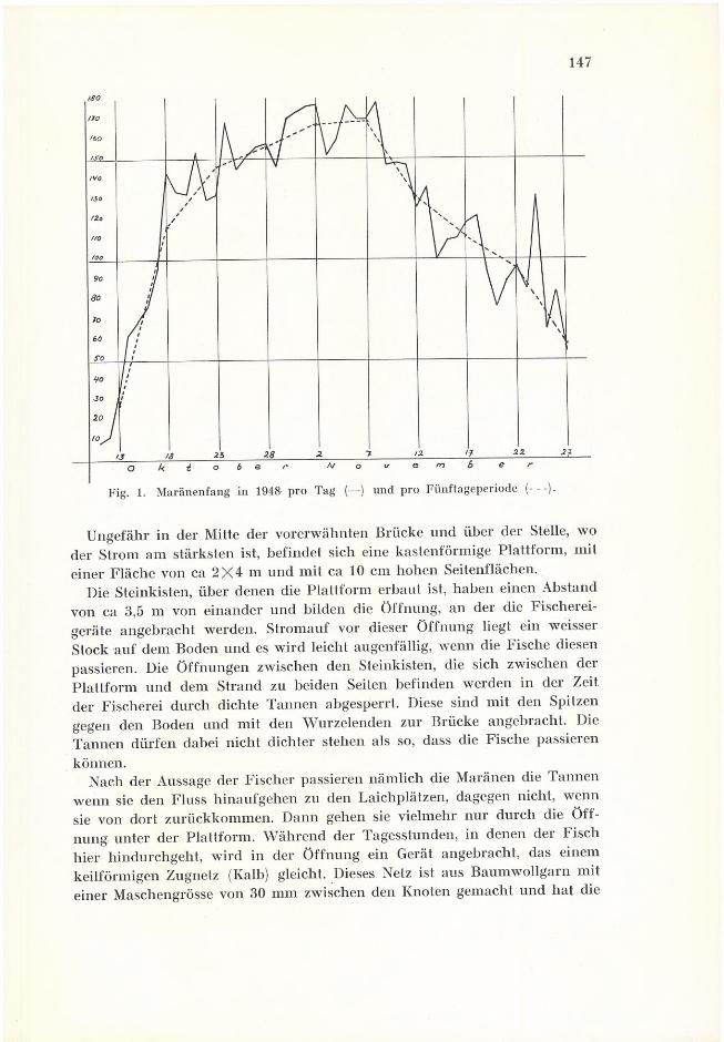
147

Fig. 1. Maränenfang in 1948 pro Tag (—) und pro Fünftageperiode (

Ungefähr in der Mitte der vorerwähnten Brücke und über der Stelle, wo der Strom am stärksten ist, befindet sich eine kastenförmige Plattform, mit einer Fläche von ca 2X4 m und mit ca 10 cm hohen Seitenflächen.

Die Steinkisten, über denen die Plattform erbaut ist, haben einen Abstand von ca 3,5 m von einander und bilden die Öffnung, an der die Fischerei­geräte angebracht werden. Stromauf vor dieser Öffnung liegt ein weisser Stock auf dem Boden und es wird leicht augenfällig, wenn die Fische diesen passieren. Die Öffnungen zwischen den Steinkisten, die sich zwischen der Plattform und dem Strand zu beiden Seiten befinden werden in der Zeit der Fischerei durch dichte Tannen abgesperrt. Diese sind mit den Spitzen gegen den Boden und mit den Wurzelenden zur Brücke angebracht. Die Tannen dürfen dabei nicht dichter stehen als so, dass die Fische passieren können.

Nach der Aussage der Fischer passieren nämlich die Maränen die Tannen wenn sie den Fluss hinaufgehen zu den Laichplätzen, dagegen nicht, wenn sie von dort zurückkommen. Dann gehen sie vielmehr nur durch die Öff­nung unter der Plattform. Wahrend der Tagesstunden, in denen der Fisch hier hindurchgeht, wird in der Öffnung ein Gerät angebracht, das einem keilförmigen Zugnetz (Kalb) gleicht. Dieses Netz ist aus Baumwollgarn mit einer Maschengrösse von 30 mm zwischen den Knoten gemacht und hat die

148

Form eines spitzenauslaufenden Beutels mit einer Öffnung von 3,5X1,5 m und einer Länge von ca 6 m. Vor Zeiten bestand dieser Keil wie die Orts­bewohner erzählen, aus einer Ledertute mit enganeinandersitzenden Löchern. Die Öffnung des Netzes ist festgemacht an einem groben Seil. Es wird zwi­schen den Steinkisten mittels zweier Stangen ausgespannt, die vom Boden bis ein Plattform reichen und dortselbst durch die Strömung festgehalten werden. Ein Gestell von Holzstangen, das vor der Netzöffnung angebracht wird, beruhigt die Wasseroberfläche, sodass die Fische, wenn sie den weissen Stock passieren, von der Plattform besser beobachtet werden können.

Die Fischerei findet, wie oben erwähnt, in den Laichzeiten um den 10. Oktober bis zum 30. November am Abend bis Einbruch der Dunkelheit und in den Morgenstunden vor der Dämmerung statt und zwar dauert jeder Fang 2 3 Stunden. Während der gesamten Laichzeit nehmen die Maränen eineununterbrochene Wanderung zwischen der See und den Laichplätzen vor. Der Aufwärtsgang geschieht in der Regel am Tage, eventuell sogar in der Nacht, die Wanderung hinunter dagegen konzentriert sich auf die Abend und Morgenstunden. Auf dieses Verhalten gründet sich die Fischereimethode. Die Fischerei wird so betrieben, dass zwei Personen, eine an jeder Stange, auf der Plattform stehen und acht geben auf den Talgang der Fische über den weissen Stock und ihr Einströmen in das Keilnetz. Wenn eine grössere Menge von Maränen in den Netzen gefangen ist werden diese hinaufgezogen und auf der Plattform entleert, worauf das Netz wieder ausgesetzt wird.

Das Bodenmaterial auf den Laichplätzen besteht hauptsächlich aus gro­bem Stein. Hin und wieder finden sich auch kleinere Stellen mit feineren Stein oder mit Kies und das scheint vor allem in der Nähe des Gittertores der Fall zu sein. Im Aussenbezirk des Laichplatzes ist auch eine gewisse Vegetation vorhanden, die hauptsächlich aus Moos, Fontinalis (nntipyretica?) aut und zwischen den Steinen auch Chara und anderen Gewächsen in unbe­deutender Menge besteht, samt den hier und dort ganz reichlich vorkom­menden Muscheln und Muschelschalen (Pisidium und Sphaerium). Die Was­sertiefe an den Laichplätzen variiert zwischen 0,2 und 1,0 meter.

Die Aufstellung, aus der der Jahresdurchschnitt der Fänge teils in Tagen teils in Fünftagesperioden zu ersehen ist, zeigt, wie die Fänge zuerst mit reell bescheidenen Ziffern beginnen, um dann schnell bis zum Kulminations­punkt zu steigen. Aus der Kurve ersieht man, dass die Fischerei ungefähr gleichzeitig mit der Wanderung der Maränen hier und zurück von den Laichplätzen beginnt und dass die Kurve nach der Kulmination, die in den ersten Tagen des November eintritt, gleichmässig aber langsamer fällt und endet, bevor die 0 Strecke erreicht ist.

Wegen Schneebehinderung und strenger Kälte hört die Fischerei in der Regel auf, bevor der Laich beendet ist und ausserdem erhält man am Ende der Laichzeit so geringe Fänge, dass die Fischerei nicht länger als lohnend angesehen wird.

149

Die Fänge während der letzten acht Jahre hatten die nachfolgende Stärke. Auskünfte über die Fischzahlen vor 1941 waren nicht zu bekommen und wahrscheinlich gibt es auch keine Aufstellung mehr.

1941 1942 1943 1944 1945 1946 1947 1948

Dur

chsc

hnitt

s­fä

nge w

ähre

nd8 Ja

hren

Stückzahl pro Jahr .........Anzahl der Fangtage.........Durchschnittstang pro Tag

516039

132

478041

116

26253771

37844584

517741

126

790246

172

364434

107

949236

264

532140

134

Wie ersichtlich schwankt die Zahl der Maränen im Jahr von 2,625 bis zu 9,492 bei einem Durchschnittsfangergebnis von 5,321 pro Jahr. Die Mittel­grösse der Maränen variiert sehr. Nach den Aussagen der Einwohner sind die Maränen in früheren Zeiten unter gewissen Perioden bedeutend geringer an Grösse gewesen, dafür aber um so zahlreicher vorgekommen. Fänge bis zu mehreren tausend Stück pro Tag sind nicht ungewöhnlich gewesen. Gerade jetzt scheint eine solche Periode begonnen zu haben. Die Mittelgrösse der Maränen in den letzten drei Jahren hat bedeutend abgenommen. Wie nut- geteilt war das Mittelgewicht der Maränen im Herbst 1946 ungefähr 300 g, im Herbst 1947 war es 211 g und im Herbst 1948 nur noch 142 g. Die mitt­lere Länge der Maränen war im Jahr 1947 30,2 cm gegen 27,1 im Jahr 1948.

Nach den Untersuchungen umfassen die Fänge folgende Jahresklassen:1947 1948

7 jährige.....................ß » .....................

................ 8 °/o3,1 °/o

5 » ..................... .................. 12 °/o 13,4 °/o

4 » ..................... .................. 62 °/o 81,4 »/o

% » ............. . . ■.................. 12 »/o 2,1 %

Wie ersichtlich, herrscht die Jahresklasse der Vierjährigen hei den Fängen mit nicht weniger als 62 % im Jahr 1947 und 81,4 °/o im Jahr 1948 vor. Alle dreijährigen Maränen waren Männchen mit rinnender Milch. Im Durch­schnitt ist das Alter des Maränenbestandes zur Laichzeit im Jahr 1948 4,17 Jahre, im Jahr 1947 — 4,36 Jahre. Das Material für die Altersbestim­mung ist von Maränen genommen in dem Verhältnis zu Grösse und Anzahl, wie sie bei den Fängen Vorkommen.

Nachfolgende Tabelle zeigt die Änderungen in der Mittelgrösse der Mara- nen bei verschiedenen Jahresklassen in den Jahren 1947—1948.

7-iälirige 6-jährige 5-jährige 4-jährige 3-jährige Total

J ahr Länge Länge Länge Gew. Länge Gew. Länge Gew.Nfi Länge Gew.

St. mm 8 St. m m 8 St. mm 8' St. mm 8 St. mm 8 < mm 8

1947 4 365 315 3 358 330 6 334 284 31 297 199 6 226 82 50 302 211

1948 3 323 252 13 296 184 79 265 132 2 234 93 97 271 142

± — — — —35 —78 — —38 —100 — —32j—67 +8 +11 — —31 —69

150

Aus der Tabelle ergibt sich, dass sieben-jährige Maränen im Herbst 1948 bei den Fängen nicht vorkamen und selbst die Zahl der sechs-jährigen war nui 50 % von der des Vorjahres. Der Zuwachs bei verschiedenen Jahres­klassen in den Jahren 1947—48 war folgender:

Länge, mm...........

19473-jährige

.............. OOß

19484-jährige

265132

+

+ 39 + 50Gewicht g ............. ............. 82

Länge mm...........4-jährige

........... 297ö-jährige

296184

— 1— 15Gewicht g ............. ............. 199

Länge mm...........5-jährige

........... 3346-jährige

323252

— 11— 32Gewicht g .............

Aus Obei stehendem geht hervor, dass der Zuwachs der 3-jährigen während des Jahres 39 mm an Länge und 50 Gramm an Gewicht betrug. Dagegen sind die Vierjährigen und besonders die Fünfjährigen sowohl an Länge wie an Gewicht zurückgegangen. Das beruht vermutlich darauf, dass das Unter- suchungsmaterial zu gering und so nicht ausschlagsgebend war, oder auch dass die geringeren Maränen eventuell an dem Laichen im Herbst 1947 nicht teilgenommen haben.

Bodenprobe von dem Laichplatz enthielten Rogenkörner und die Unter­suchung von diesen ergab folgendes Resultat:

unbefrüchtet unbestimmt10' »/o 10 °/o1,3 %> 21,3 %

In die Anzahl der Rogenkörner sind die Rogenschalen mitberechnet, und da ausserdem unbefruchtete nicht bestimmbare Rogenkörner gefunden wur­den, kann man gut annehmen, dass der Prozentsatz der Befruchtungen noch höher liegt. Die in den Proben befindlichen Rogenschalen sind mit Sicher­heit Reste von solchen Rogenkörnern, die von Insektenlarven und Boden­tieren aufgefressen wurden. In den Bodenproben befanden sich folgende Kleintiere: Trichoptera 1., Hydrophilidae 1., Hirudinea (glossifonia sp.), Svae- rium sp., Picidium sp., Oligochaeta 1., Ephemeridae 1., Diptera 1., (accephata), Limnaea sp.

Die drei erstgenannten Arten, von denen besonders Trichopteralarven in sehr grosse Menge Vorkommen, können für den Rogen schädlich sein.

Die Laichplätze sind, besonders wenn der See eisbedeckt ist, auch ein beliebter Aufenthaltort für Seevögel (Enten) welche dem Rogen in flacherem Wasser Schaden antun können.

befriichtet1947 ........................... 80 °/o1948 ........................... 77,4 o/0

151

Im Herbst 1948 machten die Vierjährigen 81,4 % von den Fängen aus. Die mittlere Länge der Jahresklasse war 32 mm kürzer und das Mittelgewicht 67 g geringer als im Herbst 1947. Man kann wohl annehmen, dass das zeiti­ger und warme Frühjahr 1945 für die Entwicklung der Brut sehr günstig gewesen ist, aber individuell haben die Maränen auf Grund der verhältnis­mässig grossen Anzahl einen ziemlich kümmerlichen Zuwachs gehabt. Die Dreijährigen machen im Jahr 1947 12 °/'o des Fangen aus und haben eine Mittellänge von 226 mm und ein Mittelgewicht von 82 g. Im Herbst 1948 kamen bei den Fängen nur 2,1 % dreijährige mit einer Mittellänge von 234 mm und einem Mittelgewicht von 93 g vor. Dieser zeigt auch, dass der Be­stand an Brut im Frühjahr 1946 kleiner war als im Jahr voraus und auf Grund dessen eine bessere Zunahme hatte.

Im Jahr 1947 lag das mittlere Fangergebnis pro Tag unter dem der letzten sieben Jahre und bei den Fängen herrschten die Jahresklasse der Vierjähri­gen vor. Man kann annehmen, dass die niedrige Fangziffer eventuell auf dem schlechten Fischbestand des Jahres 1943 beruht. In den Jahren von 1939 bis 1941 herrschte zu Laichzeit der Maränen und im Winter eine ziem­lich strenge Kälte, die, wie man sich vielleicht denken kann, auf das Aus­bruten des Rogen ungünstig eingewirkt hat und selbst auf die Möglichkeit der Brut, das erste empfindliche Stadium zu überstehen. Das traurige Fang­ergebnis 1943 bis 1944 kann auch auf den oben erwähnten Verhältnisse beruhen, da die Brut 1939—1941 im Herbst 1943 vier Jahre alt war und den Hauptteil der Laichfische ausgemacht haben durfte.

Nach der Länge und Anzahl der Kiemenreussenzähne darf man die an dem Platz vorkommenden Maränen zu den Planktonfressern zählen.

Was die Geschlechtsquote der Maränen angeht so zeigte eine Anzahl Stich­proben, dass die Männchen in der Regel in grösserer Anzahl Vorkommen. Als Durchschnittsprozentsatz bei sechs vorgenommenen Untersuchungen (zu verschiedenem Zeitpunkten) ergab sich an Männchen 57,5 % und an Weib­chen 42,5 °/o.

Geschlecht 3.11abends

4.11morgens

4.11abends

15.11abends

16.11morgens 18.11 Summe 0/o

cS................... 61 72 70 32 39 38 312 57.59................. 1 58 43 65 32 17 16 231 42.5

Wie vorstehend erwähnt, wandern die Maränen zu den Laichzeiten viele Male hin und zurück von den Laichplätzen. Deshalb kommen unter den Fängen auch Maränen, die erst halb gelaicht haben und solche mit hartem Rogen vor. Letztere Umstand machte die Berechnung des Rogens in einem Teil der Fische erst möglich.

Die Anzahl der Rogenkörner pro Maräne variiert zwischen 3,875 und 8,462 mit einer Mittelzahl von 5,865 Rogenkörner pro Maräne. Das Mittel-

152

gewicht des Rogens machte 16,1 % von dem Gewicht der Maränen oder 2,275 Rogenkörner auf jede 100 g Fisch aus. Relativ haben kleinere eventuell jüngere Maränen mehr Rogen als grössere d.h. ältere Maränen.

Die Möglichkeit Maränenrogen vor dem Rruten bei dem Fischfang zu sam­meln ist von der staatliche Fischereiversuchsstation in Kälarne seit 1931 aus­genützt worden.

Als die Rrutanstalt in Kälarne in den Jahren 1910—1920 als Privatbetrieb geführt wurde, wurde ein grosser Teil des Rogenbedarfs von der »Wach- fischerei» gedeckt. Einige Ziffern aber über die Einlieferungen waren nicht verfügbar.

Aus den Rogenberechnungen ging hervor, dass weibliche Maränen im Durchschnitt 5,865 Rogenkörner haben. Das durchschnittliche Fangergebnis pro Jahr war 4,732 Stück und im Jahr 1947 war die Anzahl der Weibchen 42,5 % von Fangergebnis. Wenn man von dieser Ziffer ausgeht, so mussten jährlich im Durchschnitt ca 1,900 Weibchen mit einer Rogenmenge von rund 11,000,000 auf gefischt werden. Da die bei den Fängen auf gefangenen Weib­chen oft mehr oder minder ausgelaicht sind und der Fang nur einen ge­wissen Prozentsatz der aufwandernden Weibchen ausmacht, ist die Rogen­menge auf dem Roden der Laichplatzes sicherlich erheblich grösser. Wie hoch der Anteil der hinaufwandernden Laichmaränen ist, der in jedes Jahr weggefangen wird, ist ohne weitere eingehende Untersuchungen schwer zu sagen.

Reports from the Institute of Freshwater Research,Drottningholm

*1933. Gunnar Aim. Statens undersöknings- och försöksanstalt för sötvattensfisket. Dess till­komst, utrustning och verksamhet. No 1. Pris kr. 0: 75.

1934. Gunnar Alm. Vätterns röding, Fiskeribiologiska undersökningar. No 2. Pris kr. 0: 75. *1934. Christian Hessle. Märkningsförsök med gädda i Östergötlands skärgård åren 1928

och 1930. No 3. Pris kr. 0: 50.1935. Gottfrid Arvidsson. Märkning av laxöring i Vättern. No 4. Pris kr. 0: 75.1935. Sten Vallin. Cellulosafabrikerna och fisket. Experimentella undersökningar. No 5.

Pris kr. 0: 75.1935. Gunnar Alm. Plötsliga temperaturväxlingars inverkan på fiskar. No 6. Pris kr. 0: 75. 1935. Christian Hessle. Gotlands havslaxöring. No 7. Pris kr. 0: 75.1935. Orvar Nybelin. Untersuchungen über den bei Fischen krankheitserregenden Spaltpilz

Vibrio Anguillarum. No 8. Pris kr. 1:25.1936. Orvar Nybelin. Untersuchungen über die Ursache der in Schweden gegenwärtig vor­

kommenden Krebspest. No 9. Pris kr. 0: 75.1936. E. Rennerfeit. Untersuchungen über die Entwicklung und Biologie des Krebspestpilzes

Aphanomyces astaci. No 10. Pris kr. 0: 75.1936. Gunnar Alm. Huvudresultaten av fiskeribokföringsverksamheten. No 11. Pris kr. 1:—.1936. Gunnar Alm. Industriens fiskeavgifter och deras användning. No 12. Pris kr. 1:50.1937. H. Bergström och Sten Vallin. Vattenförorening genom avloppsvattnet från sulfat-

cellulosafabriker. No 13. Pris kr. 0: 75.1937. Gunnar Alm. Laxynglets tillväxt i tråg och dammar. No 14. Pris kr. 0: 75.1939. Gunnar Alm. Undersökningar över tillväxt m.m. hos olika laxöringformer. No. 15.

Pris kr. 2: 50.1939. Lars Brundin. Resultaten av under perioden 1917—1935 gjorda fiskinplanteringar i

svenska sjöar. No 16. Pris kr. 1:—.1940. Nils Törnquist. Märkning av vänerlax. No 17. Pris kr. 1:—.1940. Sven Runnström. Vänerlaxens ålder och tillväxt. No 18. Pris kr. 1:—.1942. Arne Lindroth. Undersökningar över befruktnings- och utvecklingsförhållanden hos

lax (Salmo salar). No 19. Pris kr. 0: 75.1942. Lars Brundin. Zur Limnologie jämtländischer Seen. No 20. Pris kr. 2: —.1943. Gunnar Svärdson. Studien über den Zusammenhang zwischen Geschlechtsreife und

Wachstum bei Lebistes. No 21. Pris kr. 1:—.1943. Gunnar Alm. Befruktningsförsök med laxungar samt laxens biologi före utvand­

ringen. (Fertilization-Experiments with Salmon-parr.) English summary. No 22. Pris kr. 1: 50.

1945. Gunnar Svärdson. Chromosome Studies on Salmonidae. No 23. Pris kr. 3:—.1946. Arne Lindroth. Zur Biologie der Befruchtung und Entwicklung beim Hecht. (Gäddans

befruktnings- och utvecklingsbiologi samt gäddkläckning i glas.) No 24. Pris kr. 3: —.1946. Gunnar Alm. Reasons for the occurrence of stunted fish populations. (Uppkomsten

av småväxta fiskbestånd, spec, hos abborre.) No 25. Pris kr. 3: —.1947. Gösta Högström. Olika impregneringsämnens lämplighet för grovgarnig fiskredskap.

No 26. Pris kr. 1:—.1947. A. Määr. Über die Aalwanderung im Baltischen Meer auf Grund der Wanderaalmar­

kierungsversuche im finnischen und livischen Meerbusen i. d. J. 1937—1939. No 27. Pris kr. 2:—.

1947. Elias Dahr. Biologiska studier över siken vid mellensvenska östersjökusten. No 28. Pris kr. 2: —.

1949. Annual Report for the Year 1948 and Short Papers. No 29. Pris kr. 3: 50.

* Out of print.

Kr. 3: 50