From flood to drought: Transport and reactivity of dissolved ...
234
From flood to drought: Transport and reactivity of dissolved organic matter along a Mediterranean river Elisabet Ejarque Gonzalez Aquesta tesi doctoral està subjecta a la llicència Reconeixement 3.0. Espanya de Creative Commons. Esta tesis doctoral está sujeta a la licencia Reconocimiento 3.0. España de Creative Commons. This doctoral thesis is licensed under the Creative Commons Attribution 3.0. Spain License.
-
Upload
khangminh22 -
Category
Documents
-
view
2 -
download
0
Transcript of From flood to drought: Transport and reactivity of dissolved ...

From flood to drought: Transport and reactivity of dissolved organic matter
along a Mediterranean river
Elisabet Ejarque Gonzalez
Aquesta tesi doctoral està subjecta a la llicència Reconeixement 3.0. Espanya de Creative Commons. Esta tesis doctoral está sujeta a la licencia Reconocimiento 3.0. España de Creative Commons. This doctoral thesis is licensed under the Creative Commons Attribution 3.0. Spain License.

TESI DOCTORAL
Departament d’EcologiaUniversitat de Barcelona
Programa de Doctorat en Ecologia Fonamental i Aplicada
From flood to drought: Transport and
reactivity of dissolved organic matteralong a Mediterranean river
D’avingudes a sequeres: Transport i
reactivitat de la materia organica dissoltaal llarg d’un riu mediterrani
Memoria presentada per Elisabet Ejarque Gonzalez per optar algrau de Doctora per la Universitat de Barcelona
Elisabet Ejarque GonzalezBarcelona, setembre de 2014
Vist-i-plau dels directors de tesi:
Dr Andrea Butturini Dr Francesc Sabater ComasDirector Co-directorProfessor agregat, Dep. Ecologia UB Professor titular, Dep. Ecologia UB


Als meus pares


Agraıments
Voldria comencar donant les gracies a l’Andrea per haver-me animat a emprendreaquesta aventura i per haver-me encoratjat durant els alts i baixos (que han sigutmolts!). I a en Quico, per les converses de tesi sempre tant constructives. Tambe,a tota la gent del grup, especialment a l’Eusebi per estar sempre a punt per pararl’orella i fer un cafe tant llarg com calgui; a la Marta Alvarez, per les llargues con-verses que hem tingut a Fuirosos; i a l’Alba, pel seu companyerisme i pragmatisme,com dic sempre: “de gran vull ser com tu!”. Tambe vull donar les gracies a la gentdel projecte Flumed: l’Anna Romanı i l’Anna Freixa, i a l’Stefano Fazi i l’StefanoAmalfitano, pel seu optimisme i alegria durant les campanyes a la Tordera. Unacol·laboracio mediterrania que espero que nomes sigui el comencament. Tambe vulldonar les gracies a aquells que han passat pel grup de manera mes breu: Marta,Ana, Martı, pel suport que m’heu donat al laboratori i a les campanyes. And myspecial thanks to Dijana, for the great moments we shared inside and outside thelab!
Tambe vull donar les gracies a la Nuria Catalan, en Rafa Marce, en Marc Sala,i altres agosarats amb qui hem compartit les dificultats de la fluorescencia i elPARAFAC. I a en Max, per haver-me ajudat a programar la macro per fer matrius.Aixo t’ho hauran d’agrair un grapat de generacions a venir!
Seguidament vull donar les gracies a tots els companys del departament, a totssense excepcio, per crear un ambient de treball on la frontera entre feina i amistat esdesdibuixa. A la Gemma, l’Octavi, l’Isa i la Laia, per acollir-me en els meus inicis aldespatx de forestals. A la colla Manchester per l’amistat que hem anat construintal llarg de tots aquests anys: Mary, Julio, Jaime, Lıdia, Esther, Isis, Dani, Neus,Gonzalo, Eusebi, Alba, i les dues incorporacions recents, Astrid i Myrto, i segurque encara em deixo gent. Un grup on quasi tots us definiu com a rancis i, enrealitat, reconeixeu-ho: sou la gent menys rancia que he conegut mai. De conversesd’ecologia n’hem tingut ben poques, pero d’experiencies n’hem compartit mil! totsvosaltres sou el mes gran que m’ha passat aquests ultims cinc anys. Tambe vulldonar les gracies als companys de despatx, ja que conviure en un galliner no esfacil i nosaltres ho hem aconseguit: Sılvia, Anna, Ada, Nuria Catalan, Marta, Dani,
v

vi
Eusebi, Tania, Elisabet, Pau Gimenez, Claudia, Alba, Lluıs, Sandra. I tambe a enPol, en Pablo, l’Aurora, Pau Fortuno, Joan Goma, Giorgio, Nuria Sanchez, Raul,Biel, Nuria Bonada i als que ara ja esteu per paradors mes llunyans: Izaskun, Carles,Iraima, Gemma, Cesc, Oriol, Said. Gracies a tots per haver-vos creuat en el meucamı.
D’altra banda, vull donar les gracies a en Miquel Alonso per facilitar-me uncontacte que em va obrir les portes a un paıs unic: Mongolia. I would like to thankProf. Soningkhishig Nergui for giving me the opportunity to live a unique expe-rience in Mongolia. Participating in the Orkhon project has been definately themost enriching experience during my thesis. I would also like to thank Sisira With-anachchi for his friendship, professionalism, and for sharing our daily experienceswhile living abroad. Also, I have special words for Azzaya Boldbaatar, who wasalways willing to help me with the Mongolian life. And I would like to thank all theinteresting people I met within the project: the microbiologist Narantuyaa Damdin-suren, the hydrologist Tumur Sodnom, as well as all the students and professionalswho participated in the field work: Ankhbold Tsogtbayar, Enkhjin, Tseegii, Deegii,Bolortsetseg Erdenee, Tsenguun Tumurkhuyag, Tamir Tamir, Odbaatar Enkhjar-gal, among others. And finally, I would like to thank all the people that I metbesides the project which completed my Mongolian experience: Mihalis, Yannis,Thanos, Stephanie, Paula, Nara, Natsuko, Tanja, Karel, Martina, Fridi, Marceland more, thanks!
Mil gracies tambe als banyolins, per aquesta amistat que ve de lluny pero queseguim compartint amb il·lusio: Irene, Alba, Elisenda, Lıdia, Sergi, Riera, i enaquest cas sobretot a la Laura, perque en la convivencia del dia a dia tambe hasofert una part d’aquesta tesi. Gracies per escoltar-me, pels tocs a la Pedreta quanja no podia mes, pels vespres de sofa (vigila, que comenca el Karakia!). A totsvosaltres, banyolins, gracies per ser-hi!
I finalment, els agraıments mes especials son per la meva famılia. Per en Joaquimi la Mariona, per la Nuria, per l’oncle, i per l’avi i la iaia (sempre dins meu!). A totsvosaltres, gracies per fer-me sentir estimada. I els meus agraıments mes profunds,aquells que cap paraula pot descriure perque son tot sentiment, son pels meus pares.Per demostrar-me cada dia que esteu al meu costat. Sense vosaltres aquesta tesimai no hauria arribat a bon port.
Barcelona, 28 de setembre de 2014

Summary
Rivers play a key role in the global biogeochemical functioning, as they link thebiogeochemical cycles of the terrestrial and oceanic systems. In the framework ofthe carbon cycle, streams and rivers receive dissolved organic matter (DOM) froma variety of sources which is subsequently transported downstream and delivered tothe oceans. However, there is increasing evidence that this step involves not onlya relocation of DOM from the land to the seas, but also an important in-streamprocessing which modifies its quality and properties and, to some extent, outgasit to the atmosphere as CO2. However, up to now it has not been assessed howthese modifications occur along a longitudinal perspective and, most importantly,the role that hydrology plays in such downstream patterns of DOM processing.
This thesis explores the transport and reactivity of DOM along a Mediterraneanriver (la Tordera) under a variety of hydrological conditions ranging from flash floodsto summer droughts. First, the composition of DOM was determined using 3D flu-orescence spectroscopy (emission-excitation matrices) and a novel chemometric ap-proach based on a self-organising maps analysis coupled with a correlation analysis.This step allowed discerning the presence of four DOM moieties: a tyrosine-like, atryptophan-like, and two humic-like fluorescence components.
Next, longitudinal patterns of these components are presented for a range ofhydrological conditions. Along the main stem, the river exhibited three reaches witha differentiated DOM character: in the headwaters DOM had an eminent humic-like character derived from the drainage of the surrounding terrestrial catchment(high HIX); in the middle reaches (from Sant Celoni to Fogars de la Selva) therewas a predominance of the protein-like component C2 reflecting the effect of directanthropogenic water inputs (concomitant high nutrient concentrations); and thelowest part of the river was dominated by the protein-like component C1 and highFI, suggesting a predominance of microbially-derived DOM. Hydrology appearedto act as a modulator of such longitudinal patterns: during drought, the spatialheterogeneity of DOM character was maximised, whereas during flood conditionsthere was an homogenisation over the longitudinal dimension, consisting in a highlyaromatic humic-like character.
vii

viii
By means of an End-Member Mixing Analysis (EMMA) approach it was ob-served that in-stream reactive processes were likely to be driving DOM quality,especially during non-flood conditions and at the middle and lower reaches of LaTordera. Following such evidences, the relevance of in-stream transformations overtransport and physical mixing were explicitly quantified by performing a mass bal-ance approach at thirteen consecutive downstream segments. Results of the massbalance study showed that flood events, despite their brevity in time, had the ca-pacity to export the largest amounts of DOM, although having undergone littlein-stream processing. During baseflow conditions, which have been estimated tooccur annually about half of the days, there were moderate efficiencies of bulkDOM retention; however, individual fluorescence components had important in-stream generations, especially the protein-like moieties C1 and C2. In space, thisprocessing occurred in the final segments of the river, hence exhibiting a shift froma conservative to a reactive behaviour. Finally, during drought conditions the riverhad the highest capacity of DOM retention and exported the least amounts of DOM.In space, retention efficiencies were homogeneous along the mainstem, except fortwo anthropogenically-impacted sites where the retention capacities were reduced.The mass balance study also revealed that bulk DOC processing was subject toa stoichiometric control with nitrate, even though such control was weaker duringdrought.
The findings of this thesis demonstrate that the riverine passage is a decisivestep that defines the quantity and quality of the DOM that is finally delivered tothe oceans. Moreover, the observed hydrological seasonality in La Tordera shapesa temporally-changing DOM character which may have complex repercussions forits fate once in the coastal systems.

Resum
Els rius juguen un rol essencial en el funcionament biogeoquımic global, ja queenllacen els cicles biogeoquımics terrestres amb els oceanics. En el si del cicledel carboni, els rius reben materia organica dissolta (MOD) d’una gran varietatd’orıgens, la qual es transportada riu avall i alliberada al mar. Hi ha evidenciescreixents que aquest pas, no consisteix nomes en un transport conservatiu, sinoque a mes, te lloc un processat intern que en modifica qualitats i, fins a cert punt,l’oxida i allibera a l’atmosfera en forma de CO2. Malgrat tot, fins ara no s’ha avaluatcom ocorren aquestes modificacions des d’una perspectiva longitudinal, de capcaleraa desembocadura, ni el rol que la hidrologia fluvial juga en el desenvolupamentd’aquests patrons longitudinals.
Aquesta tesi explora el transport i la reactivitat de la MOD al llarg d’un riuMediterrani (la Tordera) durant un ventall de condicions hidrologiques que compre-nen des de grans avingudes fins a sequeres estivals. Primerament, es presenta unnou metode quimiometric per a determinar la composicio de la fraccio fluorescentde la MOD basat en una analisi neuronal amb mapes autoorganitzats de Kohonen.Aquesta analisi ha revelat la presencia de quatre fraccions de materia organica: unarelacionada amb la tirosina (C1), una amb el triptofan (C2), i dues amb substancieshumiques (C3 i C4).
Seguidament, es presenten els patrons longitudinals d’aquestes quatre fraccionsper un ventall de condicions hidrologiques contrastades. Al llarg del curs principal,el riu ha mostrat tres trams amb unes caracterıstiques de la MOD diferenciades:a la capcalera la MOD tenia un caracter eminentment humic i amb un HIX ele-vat, derivat del drenatge de la conca terrestre adjacent; en el tram mitja (des deSant Celoni fins a Fogars de la Selva) predominava el component proteic C2 que,coincidint amb uns elevats nivells de nutrients, reflectien l’efecte de les entradesd’aigues antropogeniques; finalment, a la part baixa del riu (des de Fogars de laSelva fins a la desembocadura) la MOD estava dominada pel component proteicC1 i un FI elevat, suggerint un predomini de substancies derivades d’una activitatmicrobiana autoctona. Amb tot, la hidrologia es va mostrar com el gran moduladord’aquests patrons longitudinals: en sequera, l’heterogeneitat espacial de la MOD
ix

x
era maxima, mentre que durant les crescudes s’esdevenia una homogenitzacio alllarg de la dimensio longitudinal, que consistia en un caracter fortament aromatic.
Mitjancant una analisi de mescla d’end-members, es va observar que la quali-tat de la MOD al llarg del curs fluvial podia estar principalment determinada perprocessos reactius autoctons, especialment fora de condicions de sequera, i en elstrams mitjans i baixos de la Tordera. Arran d’aquestes evidencies, es va quantificari discernir la rellevancia d’aquestes transformacions respecte de processos de barrejafısica. Aixo es va dur a terme mitjancant un calcul de balanc de masses en tretzesegments fluvials consecutius, localitzats entre Sant Celoni i Fogars de la Selva. Elsresultats d’aquest estudi mostren que durant les crescudes, malgrat la seva brevetaten el temps, tenen una capacitat maxima d’exportar MOD; una MOD, pero, quesofreix canvis composicionals mınims durant el seu transport. En condicions decabal basal, les quals s’estima que ocorren la meitat de dies l’any, es van observareficiencies de retencio de MOD moderades, malgrat tot, individualment pels com-ponents de fluorescencia hi van haver importants generacions, especialment per lesfraccions proteiques C1 i C2. En l’espai, aquesta generacio va tenir lloc als segmentsfinals, mostrant aixı un canvi de comportament del riu des de transportador con-servatiu a reactiu. Finalment, en condicions de sequera el riu va mostrar la maximaeficiencia de retencio, a la vegada que exportava la mınima quantitat de MOD. Enl’espai, les eficiencies de retencio es mantenien homogenies al llarg del riu, excepteen dos punts subjectes a impacte antropogenic, on les eficiencies de retencio es vanveure reduıdes. L’estudi de balanc de masses tambe va revelar que el processat delcarboni organic dissolt estava subjecte a un control estequiometric amb el nitrat,control que en condicions de sequera es va mostrar mes debil.
Els resultats d’aquesta tesi doctoral demostren que el pas fluvial es un pas decisiuque determina la qualitat i la quantitat de MOD que es finalment alliberada als mars.Aquesta estacionalitat temporal en la qualitat i quantitat de la MOD exportada,determinada principalment per les condicions hidrologiques, pot ser determinantpel destı que tindra la MOD un cop al mar.

Contents
1 General introduction 1
1.1 Characterisation of dissolved organic matter . . . . . . . . . . . . . . 1
1.1.1 Dissolved organic matter as a complex chemical mixture . . . 1
1.1.2 Fluorescence spectroscopy for the determination of DOM prop-erties . . . . . . . . . . . . . . . . . . . . . . . . . . . . . . . 2
1.1.3 Excitation-Emission Matrices and the optical landscapes ofDOM . . . . . . . . . . . . . . . . . . . . . . . . . . . . . . . 3
1.1.4 Turning spectral data into information . . . . . . . . . . . . . 4
1.1.5 Chemometric methods . . . . . . . . . . . . . . . . . . . . . . 5
1.2 The biogeochemistry of DOM in fluvial systems . . . . . . . . . . . . 7
1.2.1 Sources of riverine DOM . . . . . . . . . . . . . . . . . . . . . 7
1.2.2 Fate of riverine DOM . . . . . . . . . . . . . . . . . . . . . . 9
1.3 Downstream transport and processing of DOM . . . . . . . . . . . . 10
1.3.1 Global evidences for an active transportation of DOM in rivers 10
1.3.2 Longitudinal patterns of river function and structure: Frompredictability to stochasticity . . . . . . . . . . . . . . . . . . 11
1.3.3 The role of hydrology in DOM transport and reactivity . . . 15
2 General objectives 17
3 Materials and Methods 21
3.1 Study site . . . . . . . . . . . . . . . . . . . . . . . . . . . . . . . . . 21
3.1.1 The catchment of La Tordera . . . . . . . . . . . . . . . . . . 21
xi

xii
3.1.2 Hydrology . . . . . . . . . . . . . . . . . . . . . . . . . . . . . 24
3.2 Sampling strategy . . . . . . . . . . . . . . . . . . . . . . . . . . . . 26
3.2.1 Longitudinal sampling . . . . . . . . . . . . . . . . . . . . . . 27
3.2.2 Mass-balance sampling . . . . . . . . . . . . . . . . . . . . . . 28
3.3 Chemical analyses . . . . . . . . . . . . . . . . . . . . . . . . . . . . 29
3.4 Mass-balance calculations . . . . . . . . . . . . . . . . . . . . . . . . 32
3.4.1 Discharge measurements . . . . . . . . . . . . . . . . . . . . . 32
3.4.2 Estimation of discharge and mass fluxes from ungauged trib-utary basins . . . . . . . . . . . . . . . . . . . . . . . . . . . . 32
3.4.3 Mass balance calculations . . . . . . . . . . . . . . . . . . . . 33
3.4.4 The global mass-balance . . . . . . . . . . . . . . . . . . . . . 34
3.5 Statistical methods . . . . . . . . . . . . . . . . . . . . . . . . . . . . 36
3.5.1 EEM data mining . . . . . . . . . . . . . . . . . . . . . . . . 36
3.5.2 Multivariate analyses . . . . . . . . . . . . . . . . . . . . . . . 36
I Results: EEM data mining 39
4 Self-Organising Maps and correlation analysis for the analysis oflarge and heterogeneous EEM data sets. 41
4.1 Introduction . . . . . . . . . . . . . . . . . . . . . . . . . . . . . . . . 41
4.1.1 Self-Organising Maps . . . . . . . . . . . . . . . . . . . . . . 43
4.1.2 Correlation analysis and the determination of EEM fluores-cence components . . . . . . . . . . . . . . . . . . . . . . . . 44
4.2 Materials and Methods . . . . . . . . . . . . . . . . . . . . . . . . . . 44
4.2.1 Data set . . . . . . . . . . . . . . . . . . . . . . . . . . . . . . 44
4.2.2 Computations . . . . . . . . . . . . . . . . . . . . . . . . . . . 45
4.3 Results . . . . . . . . . . . . . . . . . . . . . . . . . . . . . . . . . . . 48
4.3.1 SOM codebooks . . . . . . . . . . . . . . . . . . . . . . . . . 48
4.3.2 Outlier sensitivity analysis . . . . . . . . . . . . . . . . . . . . 49
4.3.3 Samples projection . . . . . . . . . . . . . . . . . . . . . . . . 49

CONTENTS xiii
4.3.4 Determination of fluorescence components . . . . . . . . . . . 52
4.4 Discussion . . . . . . . . . . . . . . . . . . . . . . . . . . . . . . . . . 53
4.4.1 Next steps . . . . . . . . . . . . . . . . . . . . . . . . . . . . . 56
4.5 Conclusions . . . . . . . . . . . . . . . . . . . . . . . . . . . . . . . . 56
II Results: Longitudinal patterns of DOM quality and reactiv-ity 59
5 Preliminary assessment of spatiotemporal patterns of DOM qualityand quantity in La Tordera 61
5.1 Introduction . . . . . . . . . . . . . . . . . . . . . . . . . . . . . . . . 61
5.2 Results . . . . . . . . . . . . . . . . . . . . . . . . . . . . . . . . . . . 63
5.2.1 Hydrochemical framework . . . . . . . . . . . . . . . . . . . . 63
5.2.2 Variation in DOM concentration . . . . . . . . . . . . . . . . 64
5.2.3 Variation in DOM character . . . . . . . . . . . . . . . . . . . 65
5.2.4 Variation in DOM composition . . . . . . . . . . . . . . . . . 65
5.2.5 Differentiation of solutes and DOM content along the longi-tudinal gradient . . . . . . . . . . . . . . . . . . . . . . . . . 66
5.2.6 Relationships between variables: a multivariate approach . . 73
5.3 Discussion . . . . . . . . . . . . . . . . . . . . . . . . . . . . . . . . . 77
5.3.1 Spatio-temporal patterns of inorganic and organic solutes . . 77
5.3.2 Spatial trends of DOM quality . . . . . . . . . . . . . . . . . 78
5.3.3 Influence of hydrology on the determination of spatial trends 80
5.3.4 Next steps: Transport vs Reaction, integrating informationfrom the tributaries . . . . . . . . . . . . . . . . . . . . . . . 81
5.4 Conclusions . . . . . . . . . . . . . . . . . . . . . . . . . . . . . . . . 82
6 Multivariate exploration of DOM quality and reactivity in themain stem of La Tordera 85
6.1 Introduction . . . . . . . . . . . . . . . . . . . . . . . . . . . . . . . . 85
6.2 Results . . . . . . . . . . . . . . . . . . . . . . . . . . . . . . . . . . . 87

xiv
6.2.1 Characteristics of the tributaries . . . . . . . . . . . . . . . . 87
6.2.2 Fluorescence composition-based NMDS ordination . . . . . . 88
6.2.3 Mixing diagrams at a range of hydrological conditions . . . . 93
6.3 Discussion . . . . . . . . . . . . . . . . . . . . . . . . . . . . . . . . . 95
6.3.1 Spatio-temporal patterns of DOM composition in the mainstem . . . . . . . . . . . . . . . . . . . . . . . . . . . . . . . . 95
6.3.2 The relevance of in-stream processing . . . . . . . . . . . . . 97
6.4 Conclusions . . . . . . . . . . . . . . . . . . . . . . . . . . . . . . . . 98
III Results: Mass balance 99
7 Water balance in the middle reaches of La Tordera 101
7.1 Introduction . . . . . . . . . . . . . . . . . . . . . . . . . . . . . . . . 101
7.2 Results and discussion . . . . . . . . . . . . . . . . . . . . . . . . . . 102
7.2.1 The water inputs to the main stem . . . . . . . . . . . . . . . 102
7.2.2 Prediction of the longitudinal discharge by water balance . . 105
7.2.3 Suitability of the models . . . . . . . . . . . . . . . . . . . . . 106
7.2.4 Verification by the mass balance of a conservative solute . . . 107
7.2.5 Next steps . . . . . . . . . . . . . . . . . . . . . . . . . . . . . 108
7.3 Conclusions . . . . . . . . . . . . . . . . . . . . . . . . . . . . . . . . 108
8 Carbon and nitrogen mass balance: Linking DOC and nitrate 111
8.1 Introduction . . . . . . . . . . . . . . . . . . . . . . . . . . . . . . . . 111
8.2 Results . . . . . . . . . . . . . . . . . . . . . . . . . . . . . . . . . . . 114
8.2.1 Dissolved nitrogen concentrations . . . . . . . . . . . . . . . . 114
8.2.2 Dissolved organic carbon concentrations . . . . . . . . . . . . 115
8.2.3 Global mass balance: net function of the river . . . . . . . . . 115
8.2.4 Local mass balances: Processing heterogeneity along the mainstem . . . . . . . . . . . . . . . . . . . . . . . . . . . . . . . . 116
8.2.5 Coupling between DOC and nitrate . . . . . . . . . . . . . . 120

CONTENTS xv
8.3 Discussion . . . . . . . . . . . . . . . . . . . . . . . . . . . . . . . . . 122
8.3.1 The net function of the river . . . . . . . . . . . . . . . . . . 123
8.3.2 Inside the black box . . . . . . . . . . . . . . . . . . . . . . . 123
8.3.3 DOC mass balance . . . . . . . . . . . . . . . . . . . . . . . . 125
8.3.4 Dissolved nitrogen mass balance . . . . . . . . . . . . . . . . 126
8.3.5 Seasonal shift in the type of nitrogen retention . . . . . . . . 127
8.3.6 (Un)coupling between DOC and nitrate . . . . . . . . . . . . 128
8.4 Conclusions . . . . . . . . . . . . . . . . . . . . . . . . . . . . . . . . 130
9 Downstream processing of DOM: changes in its reactivity and com-position 133
9.1 Introduction . . . . . . . . . . . . . . . . . . . . . . . . . . . . . . . . 133
9.2 Results . . . . . . . . . . . . . . . . . . . . . . . . . . . . . . . . . . . 136
9.2.1 Fluorescence intensities of dissolved organic matter (DOM)components . . . . . . . . . . . . . . . . . . . . . . . . . . . . 136
9.2.2 Global mass balance . . . . . . . . . . . . . . . . . . . . . . . 136
9.2.3 Longitudinal profiles of retention and release . . . . . . . . . 138
9.2.4 Quantitative and qualitative coupling of DOM processing . . 140
9.2.5 Can the input characteristics of DOM determine its down-stream biogeochemical processing? . . . . . . . . . . . . . . . 143
9.3 Discussion . . . . . . . . . . . . . . . . . . . . . . . . . . . . . . . . . 144
9.3.1 Hydrology and the biogeochemical processing of DOM fluo-rescence components . . . . . . . . . . . . . . . . . . . . . . . 145
9.3.2 Relevance of different hydrological conditions in the frame-work of the Mediterranean seasonality . . . . . . . . . . . . . 148
9.3.3 Biogeochemical reactivity of DOM fluorescence components . 149
9.4 Conclusions . . . . . . . . . . . . . . . . . . . . . . . . . . . . . . . . 150
10 General discussion 151
10.1 Unveiling DOM composition: Self-Organising Maps and correlationanalysis . . . . . . . . . . . . . . . . . . . . . . . . . . . . . . . . . . 152
10.2 Flood: Inert conduit of DOM from the land to the sea . . . . . . . . 153

xvi
10.3 Baseflow: Spatial variability of DOM transport and reactivity, anddual biogeochemical role of the river . . . . . . . . . . . . . . . . . . 155
10.4 Drought: The river as a filter . . . . . . . . . . . . . . . . . . . . . . 157
10.5 The role of DOM in the regulation of inorganic nitrogen . . . . . . . 158
10.6 Implications and future research . . . . . . . . . . . . . . . . . . . . 159
11 General conclusions 161
Appendix 169
Evaluation of the capacity of DOM optical variables to quantify mix-ing processes 169
Bibliography 183

List of Figures
1.1 Excitation-Emission Matrix and location of common fluorophores . . 3
1.2 Excitation-Emission Matrix and location of optical indices . . . . . . 5
1.3 Paradigm change in the role of rivers in the global carbon cicle . . . 12
3.1 Location of the catchment of La Tordera . . . . . . . . . . . . . . . . 22
3.2 Discharge probability distribution . . . . . . . . . . . . . . . . . . . . 24
3.3 Hydrological contextualisation of sampling dates . . . . . . . . . . . 26
3.4 Longitudinal sampling design . . . . . . . . . . . . . . . . . . . . . . 27
3.5 Snapshot mass balance sampling design. . . . . . . . . . . . . . . . . 30
3.6 Conceputal models of the mass balance. . . . . . . . . . . . . . . . . 34
4.1 Summary of the SOM methodology . . . . . . . . . . . . . . . . . . . 46
4.2 Clustering of the U-matrix of the SOM analysis in the Q-mode. . . . 48
4.3 Outlier sensitivity analysis. . . . . . . . . . . . . . . . . . . . . . . . 50
4.4 Projection of space, discharge, and type of tributary onto the U-matrix. 51
4.5 Clustering of the U-matrix of the SOM analysis in the R-mode andfluorescence components determination. . . . . . . . . . . . . . . . . 52
5.1 Hydrogram of the study period . . . . . . . . . . . . . . . . . . . . . 63
5.2 Boxplot representation of the concentrations of conservative solutes . 67
5.3 Boxplot representation of the concentrations of non-conservative solutes 68
5.4 Boxplot representation of the values of DOM optical indices . . . . . 69
5.5 Boxplot representation of the volumes of EEM components . . . . . 70
xvii

xviii
5.6 Biogeochemical dissimilarity profiles . . . . . . . . . . . . . . . . . . 74
5.7 NMDS ordination based on DOM compositional dissimilarities. . . . 76
6.1 DOC and DON inputs from the tributaries. . . . . . . . . . . . . . . 89
6.2 Humic-like and protein-like inputs from the tributaries. . . . . . . . 90
6.3 NMDS showing the ordination of the end-members . . . . . . . . . . 91
6.4 NMDS showing the ordination of the main stem sites . . . . . . . . . 92
6.5 Mixing diagrams at a range of hydrological conditions . . . . . . . . 94
7.1 Longitudinal profiles of the river flow and electrical conductivity. . . 104
7.2 Longitudinal profile of infiltration. . . . . . . . . . . . . . . . . . . . 106
8.1 Theoretical framework of the stoichiometric relationship between DOCand nitrate in streamwater. . . . . . . . . . . . . . . . . . . . . . . . 112
8.2 Concentrations and mass fluxes for Nitrogen compounds . . . . . . . 117
8.3 Concentrations and mass fluxes for DOC . . . . . . . . . . . . . . . . 118
8.4 Average retention efficiencies of dissolved nitrogen and carbon solutes.120
8.5 Correlation between nitrate and DOC concentrations . . . . . . . . . 122
8.6 Retention efficiency of nitrate as a function of the DOC:nitrate ratio 124
8.7 DOC quality in the mass balance surveys . . . . . . . . . . . . . . . 128
9.1 Fluorescence intensity and fluxes for DOM fluorescence components 137
9.2 Average retention efficiencies of the fluorescence components. . . . . 140
9.3 Correlation between DOC concentration and the intensity of fluores-cence components C1 and C4. . . . . . . . . . . . . . . . . . . . . . . 141
9.4 Relationship between the processing of dissolved organic carbon (DOC)and C4. . . . . . . . . . . . . . . . . . . . . . . . . . . . . . . . . . . 142
9.5 Relationship between the processing of C4 and its initial concentrations.144
9.6 Relationship between the processing of fluorescence component C3and the values of FI and HIX optical indices at the beginning of theriver segments. . . . . . . . . . . . . . . . . . . . . . . . . . . . . . . 145
10.1 Different data mining methods applied to our EEM data set. . . . . 154

List of Tables
1.1 Bibliographic references reporting DOC losses. . . . . . . . . . . . . 14
3.1 Characteristics of the tributary basins . . . . . . . . . . . . . . . . . 29
4.1 Wavelength coordinates boundaries of the fluorescence components. . 54
4.2 Characteristics of the silhouettes of a range of hierarchical partition-ings of the R-mode SOM grid. . . . . . . . . . . . . . . . . . . . . . . 55
5.1 Data of the physico-chemical parameters . . . . . . . . . . . . . . . . 71
5.2 Data of the DOM-related variables . . . . . . . . . . . . . . . . . . . 72
7.1 Water inputs to the main stem for every sampling date . . . . . . . . 103
8.1 Global mass balance for the nitrogen solutes. . . . . . . . . . . . . . 116
9.1 Commonly accepted views regarding DOM sources and lability beingchallenged in recent studies. . . . . . . . . . . . . . . . . . . . . . . 134
9.2 Global mass balance for the DOM fluorescence components. . . . . . 138
11.1 Excitation-Emission Matrices (EEMs) of the end-members and someof the intermediate mixtures. . . . . . . . . . . . . . . . . . . . . . . 173
11.2 Summary of the linear model parameters for the different variablesevaluated. . . . . . . . . . . . . . . . . . . . . . . . . . . . . . . . . . 174
11.3 Measured and predicted values for the SOM components . . . . . . . 178
11.4 Measured and predicted values for the maximal intensity of the SOMcomponents. . . . . . . . . . . . . . . . . . . . . . . . . . . . . . . . . 179
xix

xx
11.5 Measured and predicted values for spectral indices. . . . . . . . . . . 180

Chapter 1
General introduction
1.1 Characterisation of dissolved organic matter
1.1.1 Dissolved organic matter as a complex chemical mixture
The term dissolved organic matter (DOM) refers to the pool of organic moleculesthat are dissolved in water. It is ubiquitous, as it exists in all known water bodies,and it plays a key role in the global carbon cycle as it is the largest reservoirof organic carbon on Earth (Findlay and Sinsabaugh, 2003). Operationally, it isdefined as the fraction of organic molecules that passes through a filter of 0.45micrometers (McDonald et al., 2004). However, beyond this basic criterion, DOMmolecules are highly heterogeneous, presenting a large range of chemical structuresand properties (Filella, 2008). In biochemical terms, DOM is made up of two typesof molecules: On the one hand, it contains well-known and simple biomolecularcompounds, including mainly lipids, proteins and carbohydrates, and they representabout 20-40% of the total DOM. On the other hand, there is a humic fraction thatincludes large and complex molecules, rich in aromatic groups, whose chemicalstructures are very heterogeneous and not very well-known, and they representabout 50-75% of the total bulk DOM (Volk et al., 1997). These substances arethe result of the long term mineralisation and decomposition of plant and animaltissue remains through a process termed humification. These humic substanceshave been traditionally characterised by chemical fractionation, so that we candistinguish between fulvic acids – the fraction which is insoluble at pH<2 – andhumic acids – the fraction which is soluble at all pH values (Thurman, 1985). Undera physical perspective, DOM compounds span a wide range of molecular weightsusually divided into low, medium and high molecular weight. As the size range iscontinuous, thresholds between these categories are also operational. While the low
1

2
molecular weight fraction, including the well-known biomolecules, are in the rangeof <1kDa, high molecular weight humic substances can be of the order of hundredsof kDa (Vazquez et al., 2007).
1.1.2 Fluorescence spectroscopy for the determination of DOMproperties
Such compositional heterogeneity and complexity has therefore constituted a majorchallenge for the chemical characterisation of DOM. In the field of analytical chem-istry, methodologies have mainly focused at elucidating the elemental and functionalgroups composition, with techniques like Fourier Transform Infrared Spectroscopy(FTIR), Nuclear Magnetic Ressonance Spectroscopy (NMR) and Mass Spectrome-try (MS) (McDonald et al., 2004). However, these methodologies require expensiveequipment, long protocols and an important manipulation of the samples, whatlimits the popularity and applicability of these techniques.
By contrast, fluorescence spectroscopy appeared as an analytically fast, eco-nomic and straightforward method. It is based on the fact that an important partof the molecules included in bulk DOM have the capacity to fluoresce, that is, toabsorb and emit light. Whereas it is true that not all DOM molecules have thislight-interacting capacity, the pool of molecules that effectively have this propertyinclude important groups of organic substances found in natural water bodies, likehumic and fulvic acids, as well as some protein-like material containing tryptophan,tyrosine or phenylalanine. Each of these substances represents different roles inthe environment and, hence, may provide information about a variety of ecologicalprocesses regarding DOM such as origin and transformation (Hudson et al., 2007).
The reason why the above mentioned chemical groups are optically detectableis that they contain aromatic rings in their structure. Aromatic rings have looselyheld electrons that, when they are excited with incident photons, they attain ahigher energy level. This is considered the absorption or excitation process. After-wards this absorbed energy is released again in the form of light as electrons returnto their original ground state, in the so-called emission process (Lakowicz, 2006).The intensity of light absorbed and emitted at a certain wavelength (λ) is depen-dent on the specific structure and characteristics of the aromatic groups of everymolecule. Therefore the determination of the maximal wavelengths at which a sub-stance absorbs and emits light allows the identification of that substance (Lakowicz,2006). Highly aromatic humic substances emit light at the visible range of the lightspectrum, broadly between 420 and 480 nm. At high concentrations they can bedetected at naked eye by conferring a brownish or yellowish colour to the watersample. Lower aromatic humic substances appear at progressively lower emission

CHAPTER 1. GENERAL INTRODUCTION 3
Figure 1.1 – Demonstration of an Excitation-Emission Matrix and the areas ofthe most commonly reported fluorophores according to Coble (1996) and Parlantiet al. (2000).
wavelengths and, aminoacids, typically appear in the ultraviolet at 300-370 nm(Fellman et al., 2010).
1.1.3 Excitation-Emission Matrices and the optical landscapes ofDOM
A practical way of getting an image of the different kind of optically detectablesubstances that are contained in a sample is to make a full scanning over a rangeof emission wavelengths (λem) and excitation wavelengths (λex). Such measure-ments provide an optical map in which fluorescent components appear in the formof peaks. In mathematical terms, they represent fluorescence data matrices de-scribed by two independent variables: emission and excitation. For that reason,these data sets are referred to as Excitation-Emission Matrices (EEMs) (Mopperand Schultz, 1993; Coble, 1996). In Figure 1.1 there is an example of an EEM withsome typical fluorescence peaks. It should be noted here that every peak is not nec-essarily representing a single substance, but rather a pool of substances with closearomatic or optical properties (Stedmon and Bro, 2008). This applies especially inthe present case when the analyte under consideration is DOM, containing a largediversity of organic compounds which can potentially exhibit gradients of similar-ities between them (Del Vecchio and Blough, 2004). Also, fluorophores can reflectinternal processes such as quenching or intra molecular charge transfer (Del Vecchioand Blough, 2004; Boyle et al., 2009). For that reason, hereafter detected peakswill be referred to as fluorophores, with the aim to designate groups of compoundswith similar optical properties rather than a pure chemical substance.

4
1.1.4 Turning spectral data into information
While the spectrofluorometric measurements in the lab are relatively fast and straight-forward, the subsequent data treatment and interpretation is still a major challenge,as EEMs are the expression of a complex mixture of fluorescence signals and phe-nomena. Therefore it is necessary to distil the biogeochemically meaningful informa-tion out of this complex fluorescence data. Authors have used a range of approachesin order to convert EEM data sets into some simple and manageable variables orindices:
Among the earliest approaches, but still on use, is the identification of fluo-rophores by visual peak picking. Seminal papers on DOM EEMs relied on thisapproach, like in Coble (1996) and Parlanti et al. (2000), who established nomen-clatures to designate fluorophores which have been used up to current dates. Suchfluorphores and their locations are shown and described in Figure 1.1. Peaks A,C and M appear at the longer emissions and reflect humic-like compounds. A andC are considered to be terrestrially-derived as they have been found to be the pre-dominant fluorescence signature in headwater streams (Hudson et al., 2007). PeakC corresponds to highly degraded humic material, whereas peak A corresponds todiagenetically younger components (Huguet et al., 2009). By contrast, peak M hasbeen related to humic-like compounds derived from microbial activity, and have alower aromatic character (Romera-Castillo et al., 2010). On the other hand, peaksT and B correspond to the protein-like fraction of DOM, and appear at lower emis-sion wavelengths. Peak T reflects materials related to tryptophan, whereas peakB is related to tyrosine (Yamashita and Tanoue, 2003). Often, these peaks appearbimodal, with two excitation maxima (Henderson et al., 2009).
Further, ratios between peaks have been used to infer sistemic processes, usuallyby relating the intensity of any fluorophore to that of the C or α peak. The ratioT:C has been used as a tracer of anthropogenic inputs (Henderson et al., 2009) likeurban and industrial sewage (Baker, 2001; Borisover et al., 2011) and farm wastes(Baker, 2002; Naden et al., 2010), based on the idea that impacted waters have amore predominant composition in tryptophan-like materials compared to humic-likeones. On the other hand, the ratio α’:α has been used as an indicator of the youngor mature character of the humic fraction of DOM (Coble et al., 1990; Coble, 1996;Parlanti et al., 2000). Also,γ:α gives information about the recent autochthonouscharacter of DOM and on the productivity in the aquatic environment (Parlantiet al., 2000), as the γ fluorophore has been associated with labile compounds ofprotein or bacterial origin (Yamashita and Tanoue, 2003; Cammack et al., 2004).
A similar approach to the use of fluorophore ratios are fluorescence indices, inthe sense that they use some specific {λex - λem} coordinates or regions out of thewhole EEM. But, instead of relying on peak maxima, they are computed over fixed

CHAPTER 1. GENERAL INTRODUCTION 5
Figure 1.2 – Excitation-Emission Matrix and location of the fix wavelengthcoordinates used to compute the FI, BIX and HIX indices.
wavelength coordinates (Figure 1.2). The main indices used in the literature are theFI (McKnight et al., 2001), indicator of the autochthonous vs allochthonous sourceof DOM; the HIX (Zsolnay et al., 1999), indicating the degree of humification; andthe BIX (Huguet et al., 2009), related to a predominantly autochthonous origin ofDOM and to the presence of freshly released organic matter.
All the above mentioned metrics (peak intensities, ratios between peaks, flu-orescence indices) have been successfully used in a wide variety of DOM studies,however, they still hold some drawbacks: (i) peak-picking-based metrics are subjectto an inherent subjectivity for fluorophore identification, and (ii) all these metricsrely only on some few λex − λem coordinates and, therefore, there is a lack of adeeper dealing with the whole complexity of the EEM signals. These drawbackshave become more important with the increasing size of EEM data sets, triggeredby the recent advances in spectrofluorimetry and computer software and hardware.
1.1.5 Chemometric methods
Advances in spectrofluorimetric equipment have made it possible to automate theanalysis of a large number of samples, and therefore, researchers are faced with EEMdata sets of increasing sizes. Because of that, dealing with EEMs and extractingmeaningful information out of them has become increasingly more challenging. Thetraditional approaches for identifying fluorescence components, namely visual peakpicking, has become importantly limited. On the one hand, it requires a carefulinspection of every single EEM of the data set, what can be very time consumingfor large EEM data sets. Furthermore, visual peak detection is not always obvious:some peaks appear overlapped to wider or higher peaks, or can appear as shoulders

6
to other peaks. On the other hand, peak picking results among EEMs may bedifficult to compare, as peaks do not consistently appear at the same coordinates,but have some variability in its location. Because of that, it is often confusing tosee if an observed peak is a shifted version of an already identified peak, or whetherit is a new fluorophore. Therefore, visual peak picking is not really feasible for anin-depth analysis of large EEM data sets.
Because of that, a currently active field of research is devoted to find statisticaldata mining tools that can objectively separate the broad signal of the EEMs intoindividual fluorophores, or fluorescence components, out of large EEM data sets.The most notorious advance in this sense has been the adaptation of parallel factoranalysis (PARAFAC) analysis to the specific analysis of EEM data sets (Stedmonet al., 2003; Stedmon and Bro, 2008). PARAFAC is a generalisation of PCA tohigher order arrays (Bro, 1997) and mathematically separates the mixture of fluo-rescence signals contained in the EEMs into individual constituents localised at fixλex − λem wavelength pairs (Stedmon and Bro, 2008). It is based on the funda-mental assumption that fluorophores behave independently and without interactionbetween them according to the Beer-Lamberts law. That is, the observed fluores-cence signal results from the sum of the contribution of every fluorophore presentin the sample. In practice, every component represents a group of wavelengths thatvary independently to the rest of wavelengths within the data set.
PARAFAC has been successfully used in a large number of ecological studies andhas enabled important advances in the scientific knowledge about the biogeochem-ical behaviour of DOM in marine and freshwater systems (Fellman et al., 2010).However, PARAFAC has some limitations which hinder its application to someEEM data sets. First, this model assumes that all the samples in the data set in-clude the same number of fluorophores, but at different proportions (Stedmon andBro, 2008), so that every component exhibits a full compositional variability withinthe data set. Because of that, PARAFAC is well-suited for studies characterisinggradual processes of DOM modification, like samplings along gradual environmen-tal conditions or DOM removal experiments (Stedmon and Bro, 2008). However,in the environment discontinuities and heterogeneity are usually the rule (Poole,2002) and, therefore, this limitation is not trivial, especially for observational stud-ies. Also, and related to that, PARAFAC is very sensitive to the presence of outliersas it relies on a least squares approach (Brereton, 2012). Because of these limita-tions, DOM studies have to adapt their experimental and sampling designs in orderto be able to apply PARAFAC, and this means, mainly, to focus on capturing grad-ual changes, and avoid heterogeneity, something that cannot be foreseen beforehandin most ecological studies. Therefore, in order to further advance the understandingof DOM biogeochemistry, it is necessary to further develop statistical tools that are

CHAPTER 1. GENERAL INTRODUCTION 7
less dependent on the homogeneity/heterogeneity of DOM composition, and thatare less sensitive to the presence of outliers within the data set.
1.2 The biogeochemistry of DOM in fluvial systems
In ecological terms, DOM has been considered to be one of the most importantvariables that define the function and structure of freshwater ecosystems (Prairie,2008). DOM is the most important active reservoir of organic carbon in aquaticenvironments (Findlay and Sinsabaugh, 2003), and has a fundamental ecologicalrole, as it is implied in numerous processes which control resources availability toorganisms. Namely, it mediates the transport and availability of nutrients (Taylorand Townsend, 2010) and metals (Brooks et al., 2007; Elkins and Nelson, 2002) toaquatic organisms, controls light-depth penetration and therefore light availabilityto autotrophs (Foden et al., 2008) because of its strong light absorbance capacity,and is a carbon and energy source for heterotrophic bacteria (Findlay, 2010).
During its transport along a riverine channel, DOM flows along changing envi-ronmental conditions and, consequently, becomes successively involved in differentbiogeochemical processes. Because of this interactivity, not only DOM quantity butalso its quality is susceptible to change during its transport across the landscape(Jaffe et al., 2008). The quality of riverine DOM is mainly dependant on its source,and on the subsequent transformation processes it has undergone. The main DOMsources include allochthonous (terrestrially-derived), autochthonous (in-stream pro-duced) or anthropogenic origins. Posterior transformations of DOM during its pas-sage through the riverine system depend i) on the susceptibility of a given moleculeto be transformed by a determined biogeochemical process, which can be biotic– like microbial degradation – or abiotic – like photodegradation; and ii) on thepresence of the favourable environmental conditions needed for that process to takeplace.
1.2.1 Sources of riverine DOM
Allochthonous or terrestrially-derived DOM Typically the main source ofDOM in streams and rivers originates from the drainage of the surrounding ter-restrial catchment, and therefore it exhibits eminently a composition reflectingterrestrially-derived materials, that is, humic substances resulting from the humifi-cation of lignin-derived compounds in soil (McDonald et al., 2004). The prevalenceof terrestrial DOM in the river depends firstly on its generation in the interstitialwater in soils and, secondly, on precipitation events which flush this DOM from soilsto the river. Temperature is a key factor in determining the rate of organic matter

8
decomposition (Christ and David, 1996) and hence, the production and availabilityof DOM in soil for its subsequent drainage to the stream (Freeman et al., 2001).Soil type (Clark et al., 2004) and land use (Wilson and Xenopoulos, 2009) may alsogenerate spatial variation in the generation of DOM, for example, crops have beenfound to produce compounds with less structural complexity than those of forestedareas (Wilson and Xenopoulos, 2009). But, ultimately, precipitation events consti-tute the decisive factor which controls to what extent this dissolved organic carbon(DOC) contained in soil will be effectively introduced to the river flow (Harrisonet al., 2008).
Autochthonous or in-stream derived DOM In-stream biological processesconstitute an authochthonous source of DOM. DOM can be released to the riverwater mainly by phytoplankton (Romera-Castillo et al., 2010) and macrophytes(Lapierre and Frenette, 2009), but also by microbial cell lysis, or spillage fromdamaged cells (Bertilsson and Jones, 2003). Even though this input pathway isoften overlooked for rivers and streams, it can account for 40 to 80% of DOM sourcesacross biomes (Webster and Meyer, 1997), especially when light availability is highand the surrounding catchment is poorly vegetated, as in arid areas. In general,autochthonously-derived DOM consists of simple and well known compounds suchas lipids, polysaccharides, nucleic acids and aminoacids. Also, a release of humicsubstances of low molecular weight and low aromatic content has been observed(Romera-Castillo et al., 2010). At the same time, even if it can often represent aminor fraction of whole DOM in quantitative terms, it has been observed to be ahighly labile fraction that support high rates of bacterial growth and therefore israpidly utilized (Giorgio and Pace, 2008).
Anthropogenic DOM In catchments with a high human pressure, anthropogenicactivities may significantly alter the quality and quantity of DOM flowing in a river.Such alteration can be caused, on the one hand, by the modification of land useswithin the catchment and, on the other hand, by the direct spillage of sewage ef-fluents to the river flow. Land use alteration creates a diffuse effect which altersthe quality of the terrestrially-derived DOM which is drained from the soils dur-ing storm events. Numerous studies have recognised differentiated DOM qualitiesbetween agricultural and forested subcatchments (Wilson and Xenopoulos, 2009;Williams et al., 2010). Alternatively, direct inputs from waste water treatmentplants (WWTPs), industries and urban sewage constitute point sources of anthro-pogenic DOM, whose composition can widely vary according to the kind of humanactivity that has originated it. However, some general traits have been observedthat differ those of the DOM naturally flowing in the water, such as a higher con-

CHAPTER 1. GENERAL INTRODUCTION 9
tribution of molecules resulting from bacterial activity and a higher proportion ofprotein-like material with respect to materials of humic nature.
1.2.2 Fate of riverine DOM
Once in the river water, the DOM coming from any of the above mentioned sourcesconstitutes a complex bulk DOM mixture that is transported downstream and be-comes successively involved in different biogeochemical processes – while still con-tinuously receiving new inputs of DOM molecules. Here follow the main biogeo-chemical interactions in which DOM is involved.
Microbial DOM oxidation Heterotrophic bacteria essentially control DOMtransformations, as they are the only biological compartment that can relevantlyutilize it. This pathway represents the re-introduction of matter and energy tohigher trophic levels and can be viewed as a recycling pathway of organic matterwithin the ecosystem (Azam et al., 1983). Bacteria can easily uptake the sim-ple DOM compounds by transferring them directly through their membranes usingpermease enzymes; however more complex humic compounds have to be previouslyhydrolised by means of exoenzymatic enzimes (Montuelle and Volat, 1993). As aresult of the bacterial degradation, DOM may be completely oxidised to CO2, hencebeing completely removed from the river. For instance, in the Hudson River, bac-teria have been found to be responsible for the removal of 20% of the DOC loads(Maranger et al., 2005). However, DOM can also be transformed into subproductsof lower molecular weight and higher recalcitrance (Amon and Benner, 1996). Be-cause of that, microbes are not only controllers of DOM concentration in rivers,but also have the capacity to modify its composition and character, hence affectingthe quality of the DOM that is finally delivered to oceans (Guillemette and delGiorgio, 2012). On the same time, controls on the opposite direction have beenobserved, so that bacterial communities may adapt their composition and functionto the available DOM (Docherty et al., 2006; Judd et al., 2006). This highlights thetight coupling and complex interactivity that exists between the DOM pool and thecharacteristics of the bacterial communities.
Photochemical degradation During the riverine transit, the coloured fractionof DOM has been found to selectively decay (Weyhenmeyer et al., 2012). Due to itschemical ability to interact with light, the exposure of DOM to sunlight results in adecrease in the average molecular weight (Bertilsson and Tranvik, 2000) and directmineralisation to CO2 (Miller and Zepp, 1995). Kohler et al. (2002) reported lossesof riverine DOC of 33-50%. Other fractions may not be totally mineralised butundergo profound qualitative changes (Moran et al., 2000), like a loss in the aro-

10
matic carbon functionality (Osburn et al., 2001) and a change in the proportion ofhumic substances (Kohler et al., 2002). While both the humic- and the protein-likefractions are prone to photochemical degradation, fulvic acids have been found tobe more susceptible (Mostofa et al., 2007). Some authors argue that photochemicalsubproducts are more labile than the original DOM compounds, so that it wouldfavour the biological uptake of DOM (Moran and Zepp, 1997). However, other stud-ies have found a decrease in the biodegradability of DOM due to sunlight exposure,therefore the predictability of the effects of solar radiation to DOM availability isnot yet well understood (Moran and Covert, 2003). However, photodegradation iswell-recognised as a major pathway of DOM removal and transformation withinrivers (Mostofa et al., 2007).
Other abiotic processes Microbial and photochemical degradataion and oxida-tion are the main pathways of DOM removal and transformation in rivers. How-ever, DOM interacts in a variety of additional abiotic processes. For instance, DOMmolecules may aggregate onto particulate organic matter (POM) particles (McK-night et al., 2002) and, furthermore, DOM molecules themselves may aggregateabiotically and form larger particles. Although it has not been tested in naturalconditions, laboratory experiments indicate that it can be an important processwhich can consume up to 7 – 25% of DOM, at similar taxes as those observedfor microbial uptake (Kerner et al., 2003). On the other hand, DOM also has thecapacity to bind with free metal ions through complexation, thus decreasing thetoxicity for aquatic organisms (Al-Reasi et al., 2011).
Overall, these examples highlight the wide range of interactions in which DOM isinvolved during the riverine transit. All of them occur at varying degrees of relevanceaccording to changing physical and environmental conditions found downstream asDOM flows across the landscape (Jaffe et al., 2008).
1.3 Downstream transport and processing of DOM
1.3.1 Global evidences for an active transportation of DOM inrivers
Rivers play a key role in the global biogeochemical functioning, as they link the bio-geochemical cycles of the terrestrial and oceanic systems. As mentioned, streamsand rivers receive DOM from a variety of sources and, once in the river, these com-pounds are transported downstream and delivered to oceans. Traditionally, globalmodels considered this step just as a transfer of matter from the land to the oceans.However, there are increasing evidences that important biogeochemical interactions

CHAPTER 1. GENERAL INTRODUCTION 11
occur during the downstream transport, so that rivers act as filters (Bouwmanet al., 2013) – as they retain DOM –, as well as bioreactors (Cole et al., 2007) – asthe magnitude of DOM retention evidences that complex in-stream biogeochemicalprocesses occur (Figure 1.3).
Recent models consistently estimate that rivers discharge between 0.8-0.9 PgC/yto the sea. However, there is an important variability in the estimations of the exportof carbon from the land to the inland waters, ranging from 1.7 PgC/y (Ciais et al.,2013) to 2.7-2.9 PgC/y (Cole et al., 2007; Battin et al., 2009) and 5.7 PgC/y (Wehrli,2013). This uncertainty is translated into variable estimates for carbon outgassingfrom freshwater systems as CO2 to the atmosphere (ranging from 1 PgC/y in Ciaiset al. (2013) to 4.2 PgC/y in Wehrli (2013)) and retention by burial into sediments(ranging from 0.2 PgC/y in Ciais et al. (2013) to 0.6 PgC/y in Wehrli (2013)).Despite such variability and uncertainty among models, all of them emphasize thatan important proportion of the carbon is either retained or mineralised during theriverine transit. Indeed, such estimated carbon emissions to the atmosphere aresimilar in magnitude to global terrestrial net production and, also, burial in inlandwater sediments exceeds organic carbon sequestration in the ocean floor (Tranviket al., 2009). If we consider that most of the exported C is in the form of DOM(Ludwig et al., 1996; Karlsson et al., 2005), then these figures emphasize the rolethat lotic systems have on the active transport of DOM. This points at rivers asinteresting targets at which management strategies for climate change mitigationshould be addressed (Battin et al., 2009).
1.3.2 Longitudinal patterns of river function and structure: Frompredictability to stochasticity
The global evidences that rivers act as sinks for DOM highlight the importanceof understanding the biogeochemical behaviour of DOM during the fluvial transit,from the headwaters to the river mouth. Rivers, because of their unidirectionaland longitudinal flow, are unique among freshwater ecosystems. The longitudi-nal dimension defined by the advective water transport constitutes the main axisalong which functional and structural riverine changes occur (Wipfli et al., 2007),and therefore, it is the main dimension along which changes in DOM sources andprocessing occur.
In this line, the river continuum concept (RCC) (Vannote et al., 1980) alreadypredicted fundamental changes in the carbon processing from the headwaters to theriver mouth. This model of the fluvial functioning has been very influential as itprovided a base for a holistic view of rivers by integrating a variety of concepts fromthe physical template, biological function and structure and metabolism. The RCCdescribed rivers as predictive gradients of physical and hydrological conditions which

12
Figure 1.3 – Paradigm change in the role of rivers in the global carboncycle. A) From Sarmiento and Gruber (2002), the amount of carbon deliveredto the sea by rivers is exactly the sum of the exports from the terrestrial andatmospheric systems to the river. B) From Wehrli (2013), in-stream retention andmineralisation of carbon is taken into account.

CHAPTER 1. GENERAL INTRODUCTION 13
determined a longitudinal distribution of biological communities. For carbon, itpredicted a downstream decrease in the size of organic matter, as well as a decreasein the diversity of soluble organic compounds. This trend was attributed to themicrobial degradation of the labile moieties, remaining a recalcitrant fraction up tothe river mouth.
The RCC was soon after put into question for being over simplistic, as it ignoredmuch of the spatial complexity that rivers actually have (Statzner and Higler, 1985;Sedell, 1989). Hence, a series of conceptual models further refined RCC by incor-porating elements of stochastic spatial complexity. Namely, (Ward and Stanford,1983) described the effects of dams and impoundments in disrupting the river con-tinuum, and Rice et al. (2001) pointed at tributary confluences as modifiers of theriver continuum. The magnitude of the disruptive effects have been associated withthe relative size of the tributaries with respect to the main stem (Rice et al., 2006),and may entail consequences on the river geomorphology (Benda et al., 2004), habi-tat complexity and hence biodiversity (Kiffney et al., 2006), and biogeochemicalrates (McClain et al., 2003; Fisher et al., 2004). Biogeochemically, tributaries mayintroduce water with a differentiated chemical composition with respect to the mainstem. If this new water introduces complementary or missing reactants, then theconvergence of both flowpaths may trigger the onset or accelerate the rate of cer-tain biogeochemical processes (McClain et al., 2003). In this context arouse theconcept of patchiness, and it was suggested that rivers, instead of continuum gradi-ents, should be better conceptualised as a mosaic of patches (Naiman et al., 1988;Thorp et al., 2006). As the distributions of confluences are specific to every rivernetwork, these studies reflected that stochasticity plays a main role in determininglongitudinal patterns of the riverine function and structure.
Despite the large number of conceptual studies that directly or indirectly pre-dict longitudinal changes for DOM, the empirical assessment of DOM downstreamtransformations are seldom. Some studies found an increase in the DOC concen-tration downstream (Naiman et al., 1987; Massicotte and Frenette, 2011), whereassome others found a decrease (Temnerud et al., 2007) or a steady evolution (Bat-tin, 1998). The inflow of deep groundwater was found to cause a decrease in DOCconcentrations (Nakagawa et al., 2008; Brooks et al., 2007) whereas inputs from thecatchment flushing (Nakagawa et al., 2008) and evaporation (Jacobson et al., 2000)caused an increase. Also, in some studies an increase in the variability of DOCconcentration was observed in the final part of the river (Battin, 1998; Baker andSpencer, 2004). Despite these quantitative changes, variations in the DOM qualitywere also apparent. Baker and Spencer (2004) found slight decreases in the fluores-cence intensity of humic-like components together with important increases in theprotein-like fluorophores, which they associated with anthropogenic inputs. Over-all these studies emphasize that the local characteristics and the configuration of

14
Author River SoluteSpatial
domain ∗Temporaldomain Retention †
Eatherall et al. (2000)River Swale,
UKDOC 50 km Daily scale
- 20% (3, 25and 16%)
Duan et al. (2010)Middle and
lower MississipiDON 1200 km Year scale - 12%
Dagg et al. (2005)Lower
MississipiDOC 362 km Monthly scale - 3%
Worrall et al. (2006) Peat catchment DOC 11.4 km2 Year scale - 20-32%
Worrall et al. (2007)Various UK
river networksDOC 87 - 9948 km2 Year scale - 31%
Rowson et al. (2010) Peat catchment DOC7500 and 2400
m2 Year scale+ 29 – 85Mg/km2·yr
Moody et al. (2013) River Tees, UK DOC 818km2 Year scale - 48% - 69%
Table 1.1 – Bibliographic references reporting DOC losses or production duringthe riverine transit, calculated using a mass-balance approach. * km refer to reach-scale and km2 to catchment-scale studies. † Negative values indicate losses, positivevalues indicate production.
the river network are important determinants of the longitudinal patterns of DOMquality and quantity. However, these studies do not elucidate to what extent theobserved changes are due only to the physical mixing with inflowing waters with adifferent DOM composition, or whether in-stream processing is operating.
The studies that focused on verifying the occurrence of DOM reactivity duringits downstream transport, have mostly eliminated the longitudinal view and applieda mass-balance approach at the catchment or reach level (Table 1.1). By comparingthe DOC loads introduced by the main tributaries, with those at the outlet of thecatchment, the retention of DOC can be deduced. It is common to find retentionsof 20-30% with respect to the inputs, even though there is an important variabilityamong systems (Table 1.1). These studies emphasize that the estimations at theglobal scale that rivers are sinks of DOC is also observable at the catchment level.However, while this mass-balance approach is very common to study the retentionof inorganic nutrients (Grayson et al., 1997; Salvia et al., 1999; Bukaveckas et al.,2005; Hill et al., 2010), it has been scarcely used to evaluate DOM retentivity incatchments. Moreover, most of these few experiences addressed only quantitativeterms. Qualitatively, Temnerud et al. (2009) found no relevant downstream changesin DOM optical characteristics, but (Worrall et al., 2006) found a consistent increasein the specific absorbance of DOM, although they point at an eminently conservativebalanced behaviour of DOM between the sources and sinks.
Hence, in the literature there are few studies that assess the reactivity of DOMalong a riverine continuum, but their results show that the net balance of DOM inindividual catchments, and the relevance of the role of rivers as DOM sinks remainsunclear.

CHAPTER 1. GENERAL INTRODUCTION 15
1.3.3 The role of hydrology in DOM transport and reactivity
In the previous section, most of the cited works that addressed longitudinal DOMpatterns and reactivity were performed during baseflow conditions, often becausemoderate and stable flows were considered to be the most representative (for in-stance, Temnerud et al. (2009)). However, most river systems are subject to seasonalchanges in their discharge, due to annual patterns of rainfall, snowmelt, tempera-ture, and other hydroclimatic variables. In some regions, like in the Mediterranean,flow variability includes extreme events of floods and droughts within every an-nual hydrological cycle. All the range of hydrological conditions to which a riveris subject, is necessary to fully understand its functioning (Poff et al., 1997) andbiogeochemistry (Fisher et al., 2004). Some theoretical studies acknowledged theimportance of floods and droughts as sporadic perturbations that have a determi-nant repercussion on the long-term productivity and sustainability of river systems(Naiman et al., 2008) and their ecological integrity (Poff et al., 1997).
On biogeochemical terms, floods represent a rapid flush of the terrestrial catch-ment, exporting large amounts of DOM from the land to the river flow. Dalzell et al.(2005) reported DOC exports during flood of 90 times that of baseflow conditions.The flush response of DOM to storms is well known to produce an hysteretic rela-tionship with discharge, so that DOM is more concentrated in the rising than in thedescending limb (Butturini et al., 2006). Despite these quantitative changes, stormsalso cause a change to the quality of riverine DOM. Rainfall water reactivate thedrainage of more superficial flowpaths thereby introducing freshly produced DOMcompounds that were stored in the soils (Austnes et al., 2010) to the river flow.These diagenetically-young compounds, have been reported to have an increasedavailability to stream bacteria (Fellman et al., 2009a; Wilson et al., 2013). Also,floods generate lateral exchanges with the floodplains (Junk et al., 1989) and en-hance the longitudinal continuum within the river system by a rapid downstreamtransport of water and materials.
By contrast, droughts favour the isolation of the river from the terrestrial catch-ment, so that in-stream processes become more relevant. The decrease in the al-lochthonous inputs of organic carbon and nutrients favours autotrophs, which out-compete heterotrophs (Dahm et al., 2003). Also, the longitudinal flow becomesdisrupted, thus creating isolated reaches or ponds with an independent hydrochem-ical evolution (Vazquez et al., 2011). Lower flows and longer residence times mayprovide more opportunities for the biophysical retention of DOM (Battin et al.,2008) by enhancing the contact between the water column and the river sediments.Because of that, droughts represent an important perturbation that further enhancespatial patchiness (Lake, 2000; Larned et al., 2010).

16
Overall, the importance of the hydrological variability on the river functioningand biogeochemistry has been widely acknowledged (Lohse et al., 2009); however,to what extent they specifically effect DOM downstream transport and reactivityremains unclear due to a lack of empirical studies that have addressed this issue.Moreover, these theoretical studies concerning DOM and hydrology did not considerthe longitudinal dimension. Hence, there is a lack of a concomittant perspective ofthe DOM riverine transport and reactivity in fluvial systems.

Chapter 2
General objectives
The aims of this doctoral thesis focus on the current challenge to better couplehydrological and biogeochemical research (Lohse et al., 2009). Specifically, thisthesis aims at elucidating the influence of hydrology on the longitudinal transportand processing of dissolved organic matter (DOM).
For that, research has been conducted at three successive levels, each of whichbuilds upon the previous ones:
Part I First of all, this thesis is devoted to develop a new methodology to discernindividual fluorescence components out of large Excitation-Emission Matrix(EEM) data sets that contain an important heterogeneity of spectral shapes.Specifically, this is achieved using self-organizing map (SOM) together witha correlation analysis of the component planes. The procedure is exposedin chapter 4, entitled ”Self-Organising Maps and correlation analysisfor the analysis of large and heterogeneous EEM data sets.”, and itsaims are:
• To test the suitability of Self-Organising Maps together with correlationanalysis of the component planes to analyse large and heterogeneousEEM data sets, both at the object and at the variable level.
• To test the sensitivity of this method to the presence of outliers.
• To decompose the bulk fluorescence signals of our EEM data set intoindividual fluorescence components that can be used in the rest of thethesis to study the dynamics of DOM components.
Part II Next, the focus is moved to the biogeochemistry of DOM in a Mediter-ranean river – La Tordera –, by characterizing longitudinal patterns of DOM
17

18
quantity and quality under a range of hydrological conditions. This is per-formed in two steps, corresponding to chapters 5 and 6, and the specific ob-jectives of each of them are:
For chapter 5, entitled ”Preliminary assessment of longitudinal pat-terns in the main stem of La Tordera: Hydrochemistry and DOMquality”:
• To provide a general biogeochemical description of the river.
• To assess longitudinal gradients of DOM quality and composition alonga riverine course.
• To test how contrasting hydrological conditions alter or influence thelongitudinal gradient.
• To provide a further understanding about how space and hydrology op-erate as inter-dependant dimensions of DOM quality.
In chapter 6, entitled ”Multivariate exploration of DOM quality andreactivity in the main stem of La Tordera”, more specific evidencesfor non-conservative transport of DOM are searched. Specifically, the aimsinclude:
• To explore spatio-temporal variation in the DOM composition, and therelationships between the fluorescence components and other optical andchemical variables.
• To evaluate to what extent the DOM composition observed in the mainstem can be explained as solely the physical mixing of input tributariesor, by contrast, whether in-stream processing may be operating.
Part III Finally, we use mass-balance calculations along the middle reaches of LaTordera (26 km long), and under a range of hydrological conditions, in orderto quantify changes in DOM quantity and quality. Mass-balance calculationsare used under two approaches: global, considering the whole middle part ofthe main stem as a single black box, and local, with the aim to recuperatethe longitudinal view and characterize DOM processing along the river reach.This is developed across chapters 7, 8 and 9.
Chapter 7, entitled ”Water balance in the middle reaches of La Tordera”has the aim to validate the hydrological data used to calculate the mass bal-ances of the following chapters by specifically assessing whether
• the observed discharge in the main stem corresponds to the inputs fromthe upstream tributaries or if, on the contrary,

CHAPTER 2. GENERAL OBJECTIVES 19
• exchanges with the alluvial aquifer are involved.
Chapter 8, entitled ”Carbon and nitrogen mass balance: Linking DOCand nitrate” explores the coupling between DOM quantity (i.e. DOC andDON concentrations) and inorganic dissolved nitrogen. The specific aims are:
• To compare the reactivity of bulk DOM (DOC and DON) and dissolvedinorganic nitrogen (nitrate and ammonium) along the middle reaches ofLa Tordera, and under a range of hydrological conditions.
• To test if the stoichiometric control between DOC and nitrate observedthroughout Earth’s major freshwater ecosystems (Taylor and Townsend,2010) also applies in Mediterranean systems, including extreme hydro-logical events.
• To complement the evidences for any stoichiometric control betweenDOC and nitrate with the DOC reactivity data provided by the massbalance calculations.
Finally, chapter 9, entitled ”Downstream processing of DOM: changesin its reactivity and composition” explores the transport and reactivityof individual DOM fluorescence components.
• To explore spatial patterns of the reactivity of fluorescence DOM com-ponents under contrasting hydrological conditions.
• To compare the productions/retentions observed for the individual fluo-rescence components with those of bulk DOC and DON reported in theprevious chapter.


Chapter 3
Materials and Methods
3.1 Study site
3.1.1 The catchment of La Tordera
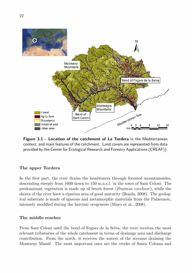
The catchment of La Tordera lies in the nort-eastern part of the Iberian Peninsula,in the central part of the catalan coast. It drains an area of 870 km2 in the Prelitoralmountain range, covering the south-eastern slopes of the Montseny and Guilleriesmountains, the northern slopes of the Montnegre, as well as part of the catalanPrelitoral depression. Its topography includes an important elevation gradient andaspect range. This has caused the development of a large diversity of landscapeswhich include the totality of the plant communities of western Europe (Bolos, 1983).In general, forest land cover dominates in the catchment (77%), especially in theupper parts. However, agriculture (16%) and urban areas and industry (7%) alsohave an important presence, especially in the lowland (Figure 3.1).
Because of the pluvial origin of the river, it is not possible to assign a specificsource point, however the popular knowledge locates the beginning of La Tordera inthe Font Bona source (broadly at 1600 m.a.s.l), in the creek of Sant Marcal, near thepeaks of Les Agudes and Turo de l’Home. From its source, La Tordera flows along60 km downstream before discharging to the Mediterranean Sea. Along its course,the river outlines sharp orographic and tectonic features, resulting in a 4-like tracecharacterised by two big bends. Such bends divide the river into three main reachesof similar length (approximately 20 km each), with distinct hydrogeomorphologicaland land cover characteristics.
21
22
Figure 3.1 – Location of the catchment of La Tordera in the Mediterraneancontext, and main features of the catchment. Land covers are represented from dataprovided by the Center for Ecological Research and Forestry Applications (CREAF)).
The upper Tordera
In the first part, the river drains the headwaters through forested mountainsides,descending steeply from 1600 down to 150 m.a.s.l. in the town of Sant Celoni. Thepredominant vegetation is made up of beech forest (Fraxinus excelsior), while theshores of the river have a riparian area of good maturity (Boada, 2008). The geolog-ical substrate is made of igneous and metamorphic materials from the Palaeozoic,intensely modified during the hercinic orogenesis (Mayo et al., 2008).
The middle reaches
From Sant Celoni until the bend of Fogars de la Selva, the river receives the mostrelevant tributaries of the whole catchment in terms of drainage area and dischargecontribution. From the north, it receives the waters of the streams draining theMontseny Massif. The most important ones are the creeks of Santa Coloma and

CHAPTER 3. MATERIALS AND METHODS 23
Arbucies, followed by the creeks of Breda, Gualba and Pertegas. Some of thesetributaries bring the waters of waste water treatment plants (WWTPs) or industriesreceived upstream. Most remarkably, the creeks of Pertegas and Arbucies receivea WWTP outlet just some few meters before discharging to the main stem. Fromthe south, the river receives the streams draining the Montnegre Mountains. In thiscase, waters are nearly pristine, as human activities and settlements are minor inthese slopes.
Contrastingly to the upper parts of the river, in the middle reaches the anthro-pogenic impacts are frequent and intense. This region hosts most of the economicactivity of the nearby territory. Hence, here aggregate industrial zones, urban set-tlements and transportation routes; namely a highway, a secondary road, a railway,as well as an oil and desalination pipeline. This has resulted in a deep modifica-tion and alteration of the riparian areas. Also, the direct discharge of industrialand WWTPs effluents affects the hydrochemical characteristics of the river water(Mas-Pla and Mencio, 2008).
From a hydrogeological perspective, in the transition from the upper to themiddle Tordera, starts the formation of sandy deposits which appear along the mainstem until its final discharge to the sea. These deposits are recent non-consolidatedquaternary materials related with the sedimentary fluvial dynamics. Their depthincreases gradually downstream, from 15 m in Sant Celoni, up to 30 m in Fogarsde la Selva, 40 m in the city of Tordera, and finally achieving 75 m in the coastline(Mayo et al., 2008).
The high porosity and permeability of the deposits make them an importantreservoir of groundwater that has a direct connection and coupled dynamics withthe river course.
The lowland
Finally, the last 20 km run between the bend of Fogars de la Selva and the Mediter-ranean sea, where the river finally discharges. This final part is characterised bya long alluvial plain, where the river adopts a curved and meandering trace, andhas a high connection between the surface and subsurface water. The contiguousplains are fertile due to the flooding dynamics of the river, and have facilitatedthe development of an intensive agricultural activity (Boada, 2008). In this area,where the orography is eminently plain, the river receives few tributaries. The mostimportant one is the creek of Reixac, which receives the waters of a WWTP fewmeters before the confluence with La Tordera.

24
Figure 3.2 – Discharge probability distribution, based on a ten-year data seriesin the gauging station of Sant Celoni. Black dots indicate discharge values withand exceedence probability of 5% or less; light grey dots, between 5 and 50%; anddark grey dots, between 100 and 50%. Own elaboration from data provided by theCatalan Water Authority (Agencia Catalana de l’Aigua).
3.1.2 Hydrology
Spatial variability of surface hydrology
During its course, the river of La Tordera encounters a variety of geological fea-tures. Especially, as it has been described in the previous section, from the villageof Santa Maria de Palautordera until the final mouth the river flows through an

CHAPTER 3. MATERIALS AND METHODS 25
alluvial aquifer with high permeability and transmissivity which create a close re-lationship between the surface and the subsurface flow. Monthly water balanceshave revealed that the river-aquifer relationship changes over time due to changesin the precipitation regime during the year. During the first semester of the yearthe aquifer tends to recharge the surface flow, whereas in the second semester, thesurface flow recharges the alluvial aquifer, due to low levels of water storage in theunderground after the summer drought (Negre, 2004).
Moreover, at a fine spatial scale the flow is also controled by tectonic elements.Regional faults are frequent along the main stem (Insitut Cartografic de Catalunya,2002), and control the drainage pattern (Mayo et al., 2008). In the middle reaches,the river flow eminently follows the trace of a major fault oriented NE-SW. Alongthis main fault, a series of minor faults intersect perpendicularly and may modifylocally the river-aquifer flow behaviour (Mas-Pla et al., 2013).
However, the main source of spatial variability in the water flow is the successiveconfluence with tributaries of varying discharge contribution. Especially in themiddle reaches, the river receives the waters of numerous tributaries, and the mainwater contributions occur after the confluences with the creeks of Arbucies andSanta Coloma, as they are the tributaries draining the largest sub-catchments.
Temporal variability of surface hydrology
The hydrological regime of La Tordera is influenced by a Mediterranean climate,which consists in rainy and humid autumns and springs on the one hand, anddry and warm summers on the other hand. According to that, discharge exhibitsextreme and contrasted events over an annual cycle, consisting on flood events inautumn and spring, and drought periods in summer.
Floods are usually short in time (in the order of hours to some few days), butintense in magnitude. In the gauging station of Sant Celoni, extreme dischargevalues up to 175, 203 and 267 m3/s have been calculated to occur in return periodsof 50, 100 and 267 years, respectively (Mayo et al., 2008). In a smaller time scale,including the last ten years (2003 to 2013) the hydrogram (Figure 3.2) shows theoccasional occurence of stormflows peaking around 10 m3/s, and even reaching 27m3/s in an event in 2011. However, such high flows are instantaneous responses tostorms which are rapidly flushed out of the system, and discharges higher than 2.03m3/s only occurred 5% of the days during the last decade (Figure 3.2, inset).
Contrastingly, drought periods are prolonged in time. They naturally occur insummer, between the months of july and september, and their length and severitybasically depend on the abundance of rains during the previous spring, as well as thetemperatures during summer. However, water withdrawal from the alluvial aquifer

26
Figure 3.3 – Hydrological contextualisation of sampling dates, for both the longitudinal and
the mass balance sampling designs. * Samplings based on the mass balance design, but where the
tributaries have not been exhaustively sampled; data used to complete the data sets of chapters
4 and 6. F stands for ”flood”, B for ”baseflow”, HB for ”high baseflow”, LB for ”low baseflow”
and D for ”drought”. Black dots indicate discharge values with and exceedence probability of 5%
or less; light grey dots, between 5 and 50%; and dark grey dots, between 100 and 50%, as shown
in Figure3.2. Data provided by the Catalan Water Authority (Agencia Catalana de l’Aigua).
to satisfy industrial and urban demand often accentuates the reduction of the surfaceflow. This was specifically observed for the years 2003-2005 (Mas-Pla and Mencio,2008), manifested by a convex shape of the recession curve of the hydrograph (Sala,2005). In the last decade, during 50% of the the days, the gauging station of SantCeloni registered flows of less than 0.18 m3/s, (Figure 3.2) flows which correspond,approximately, to the minimum environmental flows threshold established by theCatalan Government (which is of 0.204 m3/s in the summer months 1). Moreover,these minimal flows depend, to a large extent, on the inputs from WWTPs and otheranthropogenic effluents (Mas-Pla and Mencio, 2008). Overall, this emphasizes theextended occurrence during the year of an hydraulic deficit in the river system.
3.2 Sampling strategy
With the aim of describing biogeochemical trends and processes during downstreamriverine transport, the sampling design was focused at the main stem. Specifically,two sampling strategies were performed, hereafter referred to as longitudinal andmass balance.
1Pla sectorial de cabals de manteniment de les conques internes de Catalunya. ResolucioMAH/2465/2006, de 13 de juliol, per la qual es fa public l’Acord del Govern de 4 de juliol de 2006,pel qual s’aprova el Pla sectorial de cabals de manteniment de les conques internes de Catalunya.DOGC Num 4685, 27-7-2006, pag 33808-33821.

CHAPTER 3. MATERIALS AND METHODS 27
Figure 3.4 – Longitudinal sampling design. Ten sites were sampled along themain stem, from the river’s source, to its mouth.
3.2.1 Longitudinal sampling
This sampling designed was aimed at providing a preliminary assessment of biogeo-chemical longitudinal patterns. According to that, the main stem of La Torderawas sampled in ten sites distributed from the headwaters to the river mouth (Fig-ure 3.4), designated as sites S1 to S10. The first three sampling sites (S1-S3) werelocated between La Llavina and Santa Maria de Palautordera, that is, in the moun-tainous and forested headwaters. Next, sites S4 to S6 corresponded to the middlereaches of the river, spanning between the bends of Sant Celoni and Fogars de laSelva. Finally, sites S7 to S10 were in the lowland, were S10 corresponded to thevery final river mouth.
Samplings were conducted eight times, representing three different hydrologicalconditions: flood, baseflow, and drought (Figure 3.3). The droughts of 2009 and2010 differed in that the former had moderate rainfall antecedents whereas the latterhad flood antecedents. Every hydrological condition was sampled twice and resultswere averaged. It should be noted here that site S9 was dry during drought dates.In total, 76 samples were collected, averaged to 38.
The results of these samplings constitute the base for the study presented inchapter 5. These data are also included in the data sets used in chapters 4 and 6.

28
3.2.2 Mass-balance sampling
This sampling design was aimed at complementing the information provided by thelongitudinal sampling strategy, so that the information from the main stem couldbe contrasted with information about the tributaries that originate the flow of themain stem. The results from these samplings constitute the core of the mass balancestudy presented in chapters 7, 8 and 9.
In this sampling design, we applied a snapshot mass-balance to the middle partof the main stem, from the village of Santa Maria de Palautordera to Fogars de laSelva, comprising a total length of 26 km (Figure 3.5). This large reach was chosenbecause it is the part of the main stem which receives most of the tributaries of thecatchment, as well as a variety of water inputs, from pristine tributaries to directindustrial effluents. In addition there is no surface water extraction in this reachand the water flow is not altered by relevant morphological barriers (i.e. dams).
The snapshot mass-balance design Grayson et al. (1997) provides an instanta-neous picture of the water and mass fluxes entering and flowing out from a selectedriver reach or catchment area. For that, it is necessary to sample every confluenceduring a time period as short as possible. Hence, in this work special attention wasdevoted to sample all exisiting confluences along this 26-km reach as exhaustively aspossible (Figure 3.5). Eight major tributaries were directly sampled. These includethe creeks of Vallgorguina, Pertegas, Gualba, Fuirosos, Breda, Arbucies and SantaColoma (sites A2, A3, A5, A6, A7 and A10 in Figure 3.5, their characteristics arelisted in Table 3.1), as well as the main stem itself at the beginning of the reachafter draining the headwaters (A0, Figure 3.5). Overall they represented a directmeasure of the 85% of the catchment drainage area (Figure 3.5, dark region). Theinputs from the rest of the catchment, which remained ungauged (Figure 3.5, light-coloured region), were estimated by the average specific discharge of the collindantgauged subcatchments (see Section 3.4.2 for further details). Also, 3 anthropogeniceffluents discharging directly to the main stem were sampled. They correspondedto a WWTP (WWTP of Santa Maria de Palautordera, site A1, Figure 3.5) and twoindustries which discharged directly to the main stem (sites A4 and A9, Figure 3.5,lying in the industrial areas of Sant Celoni and Macanet de la Selva).
As to the main stem, it was sampled before every tributary junction, as well asin some additional sites where the tributary confluences were sparser. In total, mainstem sampling sites divided the whole river reach into 13 consecutive segments. Theaverage length of each segment was 1.98 km, while the longest and the shortest were,respectively, 3.22 and 0.66 km long. The last sampling site, located in Fogars de laSelva, represented the final outlet of the mass-balance system. Besides the middlereaches, the headwaters and the lowland were also sampled, in the same sites as in

CHAPTER 3. MATERIALS AND METHODS 29
the longitudinal sampling, to provide some continuity to the data series (sites S1 toS3, and S8 to S10, Figure 3.4).
This sampling was performed on four occasions between 2011 and 2013, com-prising a range of hydrological conditions: flood (156 m3/s), baseflow (3.43 and1.49 m3/s) and drought (0.065 m3/s) (discharge values corresponding to Fogarsde la Selva). Overall, these samplings spanned four orders of magnitude of riverflow, allowing to characterise a wide range of hydrological conditions (Hydrologicalcharacterisation in Figure 3.3).
3.3 Chemical analyses
Sample preprocessing
For the chemical and spectroscopic measurements, water was filtered with precom-busted GF/F filters and next with nylon 0.22µm-pore membranes. For total organiccarbon (TOC), an aliquot of 30mL was acidified 3% v/v with HCl 2M and storedrefrigerated. Besides, aliquots of 10mL were kept frozen for subsequent nutrient andion analysis. For spectroscopic measurements, 30mL aliquots were kept refrigeratedin acid rinsed glass bottles and were analysed within a maximum of 5 days.
Chemical analyses
Total organic carbon (TOC) was determined by oxidative combustion and infraredanalysis with a Shimadzu TOC Analyser VCSH. A coupled unit determined thetotal nitrogen (TN) by oxidative combustion and chemoluminescence. Ammoniumconcentration was measured using the salicylate method of Reardon (1969), and
Drainage Average slope Land use (%)Sub-catchment area (km2) (degrees) Forest Agriculture Grassland Urban Other
Headwaters 87.92 21.51 72.70 7.78 11.62 5.68 2.23Vallgorguina 36.67 14.9 73.50 8.26 4.29 10.23 3.73
Pertegas 25.35 17.96 72.21 8.87 10.07 6.06 2.79Gualba 26.08 19.69 80.53 4.59 9.19 3.71 1.98
Breda 32.37 16.68 63.71 8.99 14.69 10.78 1.84Arbucies 112.07 20.52 84.46 3.78 6.21 2.95 2.59Fuirosos 19.26 21.75 95.80 1.79 1.53 0.37 0.51
Santa Coloma 321.73 12.82 67.18 11.75 9.42 8.19 3.47
Table 3.1 – Characteristics of the tributary basins, sampled in the mass balancestudy.

30
Figure 3.5 – Snapshot mass balance sampling design, performed along a 26-kmriver reach, spanning from Santa Maria de Palautordera to Fogars de la Selva. Allrelevant water inputs along were sampled before discharging to the main stem, rep-resenting 85% of the total drainage area. Also, the main stem was sampled beforeevery confluence, as well as between confluences when tributaries were sparser.
the soluble reactive phosphor (SRF) was measured using the method of the molib-date of Murphy and Riley (1962); both methods as described in Butturini et al.(2009). Nitrates, chloride and sulphate concentrations were analysed with an ionchromatograph Metrohm 761 Compact IC with the column Metrosep A Supp5 -150/4.0. Next, dissolved organic nitrogen (DON) was estimated by the differencebetween TN and the sum of nitrates and ammonia. Nitrites were not considered asthey appeared under the detection limit of the ion chromatograph analyses.
Excitation-Emission Matrix analysis
Prior to analysis, samples were left in the dark to attain room temperature. Next,fluorescence analyses were performed using a Shimadzu RF-5301 PC spectrofluo-
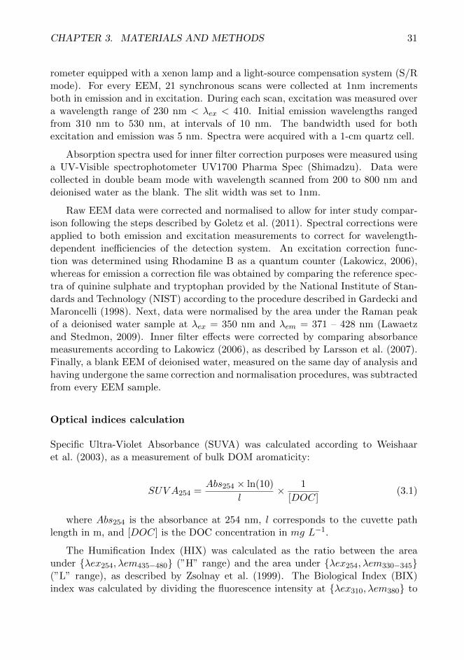
CHAPTER 3. MATERIALS AND METHODS 31
rometer equipped with a xenon lamp and a light-source compensation system (S/Rmode). For every EEM, 21 synchronous scans were collected at 1nm incrementsboth in emission and in excitation. During each scan, excitation was measured overa wavelength range of 230 nm < λex < 410. Initial emission wavelengths rangedfrom 310 nm to 530 nm, at intervals of 10 nm. The bandwidth used for bothexcitation and emission was 5 nm. Spectra were acquired with a 1-cm quartz cell.
Absorption spectra used for inner filter correction purposes were measured usinga UV-Visible spectrophotometer UV1700 Pharma Spec (Shimadzu). Data werecollected in double beam mode with wavelength scanned from 200 to 800 nm anddeionised water as the blank. The slit width was set to 1nm.
Raw EEM data were corrected and normalised to allow for inter study compar-ison following the steps described by Goletz et al. (2011). Spectral corrections wereapplied to both emission and excitation measurements to correct for wavelength-dependent inefficiencies of the detection system. An excitation correction func-tion was determined using Rhodamine B as a quantum counter (Lakowicz, 2006),whereas for emission a correction file was obtained by comparing the reference spec-tra of quinine sulphate and tryptophan provided by the National Institute of Stan-dards and Technology (NIST) according to the procedure described in Gardecki andMaroncelli (1998). Next, data were normalised by the area under the Raman peakof a deionised water sample at λex = 350 nm and λem = 371 – 428 nm (Lawaetzand Stedmon, 2009). Inner filter effects were corrected by comparing absorbancemeasurements according to Lakowicz (2006), as described by Larsson et al. (2007).Finally, a blank EEM of deionised water, measured on the same day of analysis andhaving undergone the same correction and normalisation procedures, was subtractedfrom every EEM sample.
Optical indices calculation
Specific Ultra-Violet Absorbance (SUVA) was calculated according to Weishaaret al. (2003), as a measurement of bulk DOM aromaticity:
SUV A254 =Abs254 × ln(10)
l× 1
[DOC](3.1)
where Abs254 is the absorbance at 254 nm, l corresponds to the cuvette pathlength in m, and [DOC] is the DOC concentration in mg L−1.
The Humification Index (HIX) was calculated as the ratio between the areaunder {λex254, λem435−480} (”H” range) and the area under {λex254, λem330−345}(”L” range), as described by Zsolnay et al. (1999). The Biological Index (BIX)index was calculated by dividing the fluorescence intensity at {λex310, λem380} to

32
that at {λex310, λem430} (Huguet et al., 2009). Finally Fluorescence Index (FI)(McKnight et al., 2001; Cory et al., 2010) was calculated as the fluorescence intensityat {λex370, λem470} nm divided by that at {λex370, λem520} nm.
3.4 Mass-balance calculations
3.4.1 Discharge measurements
At every sampling site, discharge was determined with the velocity-area method. Itconsists on the summation of the product between the mean velocity (ui) and cross-sectional area (A) of a series of sub-segments along a river transect (Di Baldassarreand Montanari, 2009):
Qobs =
n∑i=1
ui ×Ai (3.2)
The mean velocity for every subsegment was measured with a flow meter GlobalWater FP111, by sampling the point velocity at one half of the total depth, in themiddle of the segment width.
In flooding conditions, when the river flows were too high to take in-stream mea-surements with the flowmeter, river discharge was estimated using the Manning’sequation (Manning, 1891):
Qobs =
(1.49
n
)×A×Rh2/3 × S1/2 (3.3)
which estimates river discharge based on the cross-sectional area (A), hydraulicradius (Rh), river bed slope (S) and the Manning’s roughness coefficient (n). n wasset to values between 0.05 and 0.06 following the reference tables in Chow (1959).
3.4.2 Estimation of discharge and mass fluxes from ungauged trib-utary basins
In order to account for those small basins which remained ungauged in our sam-pling design, their discharge was estimated by the Drainage-Area Ratio (Emersonet al., 2005). This method assumes that the stream flow of ungauged basins can beestimated by using the specific discharge of a nearby gauged basin as a conversionfactor from basin area to discharge. Therefore, discharge in an ungauged basin(Qug) can be calculated as:

CHAPTER 3. MATERIALS AND METHODS 33
Qug = Aug ×Q′g = Aug ×Qg
Ag(3.4)
Where Aug is the drainage area of the ungauged basin and Q′g is the specificdischarge of a reference gauged basin. Q′g is the ratio between the discharge and thedrainage area and is expressed as m3s−1km−2. In our calculations, for every un-gauged basin we used as reference the average specific discharge of the two adjoininggauged basins.
Similarly, the mass flux from ungauged basins mug was estimated as:
mug = Aug ×m′g = Aug ×mg
Ag= Aug ×
Cg ×Qg
Ag(3.5)
where m′g is the specific mass flux of a reference gauged basin, that is, the ratiobetween the mass flux and the drainage area, expressed as mgs−1km−2. Again, inour calculations, for every ungauged basin we used as reference the average specificmass flux of the two adjoining gauged basins. For convenience, mug can also beexpressed in terms of concentration as follows:
Cug =mug
Qug(3.6)
where Qug is the discharge of that given ungauged basin, as estimated in Eq.3.4.
3.4.3 Mass balance calculations
Prior to mass-balance calculations, all the gauged and ungauged inputs joining themain stem between two given main stem sampling sites, were added. This wasmeant to facilitate the calculations, by considering a single tributary for every riversegment i:
Qtrib(i) = Qg(i) +Qug(i) (3.7)
mtrib(i) = mg(i) +mug(i) (3.8)
Next, snapshot mass balances were calculated under two perspectives: global andlocal.

34
3.4.4 The global mass-balance
In the global mass-balance approach, the river reach was conceptualised as a bigblack box (Figure 3.6-A), in which all the inputs were summed together as a singleoverall input to the system. This input was considered both in terms of water andmass flux:
Qin =13∑i=0
Qtrib(i) (3.9)
min =13∑i=0
mtrib(i) (3.10)
where Qtrib(i) and mtrib(i) correspond, respectively, to the water and mass inputsreceived in each of the 13 river segments (Eq. 3.7 and 3.8). Note that the summationstarts at 0, as tributary 0 corresponds to the water and mass flux coming from theheadwaters (Fhw in Figure 3.6). Overall, these total inputs correspond to the fluxthat we expect at the outlet of the river reach.
Figure 3.6 – Conceptual models of the mass balance. A) Global mass balanceapproach, B) Local mass balance approach. F refers to any flux, water of mass.Fhw corresponds to the inputs supplied by the main stem coming from the head-waters, Ftrib are the inputs from the tributaries, and ∆F are the exchanges withthe underlying alluvial aquifer, which can be an input or an output of the system,depending on the river-aquifer relationship at the specific time of sampling.

CHAPTER 3. MATERIALS AND METHODS 35
Any discrepancy between the water inputs (Qin) and outputs (Qout) are assumedto correspond to the amount of water that has been exchanged with the alluvialaquifer (∆Q), that is, the amount of infiltrated or upwelled water or mass duringthe 26-km downstream transit:
∆Q = Qout −Qin (3.11)
Positive values of ∆Q indicate an upwelling of water, whereas negative valuesindicate the occurrence of infiltration. The knowledge of this ∆Q is essential inorder to estimate the amount of mass that we loose or gain through water exchangewith the alluvial aquifer (∆m). In the absence of any in-stream reactive process,we can compute an expected mass flux at the outlet of the river reach as follows:
mout(exp) == min −∆m (3.12)
∆m(%) =mout(obs) × 100
mout(exp)− 100 (3.13)
At this point, any discrepancies between the expected and the observed massfluxes in the outlet (Eq. 3.13) correspond to in-stream transformation processes, asall the inputs and outputs of the river reach have been taken into account. Thus,positive values of ∆m indicate a net production or release along the river reach,whereas negative values indicate net retention processes. This provides informationabout the overall function of the river with respect to a biogeochemical compone-nent: whether it behaves as a source (production or generation predominates) or asa sink (loss or retention predominates).
The local mass-balance
In the local mass-balance approach, the river reach is split into 13 black boxes,each of them spanning two consecutive main stem sampling sites (Figure 3.6-B).These boxes are linked one another in series, in such a way that every main stemsite represents the output of its ustream black box, as well as the input to itsdownstream black box. In addition, every black box receives the inputs of anytributaries that join the main stem in that specific river segment. In essence, it isthe same approach of the global mass balance, but applied successively to differentsegments of the whole river reach. This view dissects the information provided bythe global mass balances, and allows to locate on a longitudinal axis, the spatialdistribution of production or retention processes.

36
In every river segment, inputs can be calculated as the sum of the tributariesjoining that specific river segment plus the flux coming from the upstream mainstem sampling site:
Qin(i) = Qout(obs)(i−1) +Qtrib(i) (3.14)
min(i) = mobs(obs)(i−1) +mtrib(i) (3.15)
where Qtrib(i) and mtrib(i) are the water and mass flux from the catchmenttributaries entering the system at the segment i, as defined in Eq. 3.7 and 3.8.
In every segment i, the difference between the inputs and the observed out-puts correspond to the amount of water exchanged with the alluvial aquifer (∆Q,calculated as in Eq. 3.11). Again, this ∆Q is essential in order to calculate theexpected mass flux in the outlet of every segment i in absence of in-stream pro-cessing (Cout(exp)(i)). This mout(exp)(i), as well as the percentage difference betweenthe expected and the observed mass flux at the outlet of every segment, can becalculated using the equations 3.12 to 3.13.
3.5 Statistical methods
3.5.1 EEM data mining
In order to explore patterns among EEM samples, as well as to discern and identifyindividual fluorescence components present throughout the data set, a new methodis developed in this thesis based on a type of artifitial neural network (ANN) analysiscalled self-organising maps (SOMs). Therefore, all details about this statisticalmethod are thoroughly presented in Chapter 4.
3.5.2 Multivariate analyses
In chapters 5 and 6, a non-metric multidimensional scaling (NMDS) was used in or-der to explore patterns among samples based on DOM fluorescence composition, asdetermined with SOM. An original multidimensional space, defined by the differentfluorescence components, was fit to a two-dimensional space. Computations usedBray-Curtis distances and data were previously mean-centred and scaled by theirstandard deviation. Goodness-of-fit was assessed by two correlation-like statisticswhich relate ordination distances and original dissimilarities taking into accountNMDS nonlinear transformations.

CHAPTER 3. MATERIALS AND METHODS 37
In order to aid the interpretation of NMDS results, hydrochemical solutes andDOM optical indices were fitted onto the NMDS analysis by means of a vectorfitting analysis. Those vectors that significantly fit the ordination, a) point to thedirection of maximum change and b) their length is proportional to their correlationdegree within the ordination.
NMDS and vector fitting analyses were computed using R v. 2.15 (R Develop-ment Core Team, 2012) and the associated vegan package (Oksanen et al., 2012).

38
Results Part I
EEM data mining
39


Chapter 4
Self-Organising Maps andcorrelation analysis for theanalysis of large andheterogeneous EEM data sets.
Elisabet Ejarque-Gonzalez and Andrea Butturini. Self-organising maps and cor-
relation analysis as a tool to explore patterns in excitation-emission matrix data sets
and to discriminate dissolved organic matter fluorescence components. PloS one, 9
(6), 2014. doi: 10.1371/journal.pone.0099618
4.1 Introduction
Excitation-Emission Matrices (EEMs) are three-dimensional fluorescence data thatprovide information about the composition of fluorescent chemical mixtures. Theyconstitute optical landscapes that extend over the dimensions of excitation and emis-sion wavelengths λex − λem, and where fluorophores appear in the form of peaks.In the field of marine and freshwater biogeochemistry, EEMs have been used for thestudy of dissolved organic matter (DOM), being a comprehensive analytical tech-nique with which to characterise a highly complex mixture of organic compounds(Hudson et al., 2007; Fellman et al., 2010; Nebbioso and Piccolo, 2013). Indeed,EEMs have served to advance scientific knowledge about the ecology and biogeo-chemistry of DOM in aquatic systems (Hudson et al., 2007; Fellman et al., 2010).Most importantly, they have contributed to evidence that some fractions of DOMare highly reactive organic molecules that are involved in numerous ecosystem pro-
41

42
cesses, such as bacterial uptake (Azam et al., 1983; Findlay, 2010; Cory and Kaplan,2012), metal binding (Elkins and Nelson, 2002; Brooks et al., 2007), photoreactiv-ity (Bertilsson and Tranvik, 2000; Mostofa et al., 2007; Osburn et al., 2009) andlight attenuation (Foden et al., 2008). Overall these findings suggest the majorinvolvement of DOM in the global carbon cycle (Cole et al., 2007; Tranvik et al.,2009).
Despite the great potential for EEMs to increase knowledge about DOM be-haviour in the environment, their interpretation and statistical treatment remaina challenge (Bieroza et al., 2011). The spectral shapes of EEMs are complex mix-tures of multiple and overlapping independent fluorescence phenomena, caused bythe wide range of organic molecules contained in DOM. As only about 25% of thesemolecules have been identified (Benner, 2002), there is a lack of chemical standardsto be used to separate the signal of bulk DOM into its individual components. Forthat reason, there is a need to develop pattern recognition methods capable of de-tecting and isolating the signal of different fluorescing moieties in the absence ofany previous knowledge about the composition of DOM in a given sample.
A well-suited tool to satisfy these needs are self-organizing map (SOM). SOMis an artificial neural network algorithm that mirrors the biological brain function(Kohonen, 2001). Due to its unsupervised self-learning capacity, it is capable ofrecognizing patterns in complex data sets without following any assumptions aboutthe data structure. Although it has been increasingly used within analytical chem-istry in recent years (Brereton, 2012) it has not been until recently that SOM hasbeen used to analyse EEM data sets (Bieroza et al., 2009, 2012), and the potentialfor SOM to equate or even outperform other state-of-the-art EEM data treatmentmethods like partial least-squares regression (PLS), principal components analy-sis (PCA) and parallel factor analysis (PARAFAC) has been highlighted (Bierozaet al., 2011; Brereton, 2012; Lloyd et al., 2008; Bieroza et al., 2012). The map spaceproduced by SOM offers multiple possibilities for the graphical representation ofthe output, allowing to unveil patterns among samples (best matching unit andunified distance matrices), as well as to explore what variables (wavelength coordi-nates in the case of EEM data sets) are the most influent in creating the samplepatterns (component planes) (Brereton, 2012). However, pattern recognition at thevariable level has remained at a qualitative stage, and the specific need to isolateindependent fluorophores has not been covered.
Furthermore, previous analyses of EEM data sets with SOM were performed ondata from engineered systems, where the diversity of fluorophores was essentiallyhomogeneous among the samples (Bieroza et al., 2009, 2012). However, EEM datasets collected in natural water systems are subject to contain a wide diversity ofspectral shapes, due to the multiple environmental factors that influence DOMquality (Jaffe et al., 2008). In this case, data pattern interpretation may become

CHAPTER 4. SELF-ORGANISING MAPS 43
more challenging, as the presence of outliers may alter the stability of the SOMoutput, and hence its reliability.
In this context, this study aims at expanding the evidences that SOM is asuitable tool for the study of EEM data sets. Specifically, we focus on two aspects.On the one hand, we aim to further test the performance of SOM when a highheterogeneity of spectral shapes is contained within the data set. We address thispoint by assessing the stability of the quantization and the neighbourhood relationsof the SOM output under a leave-one-out cross-validation approach. On the otherhand, we search for independent fluorophores by extending SOM with a correlationanalysis of component planes. This constitutes a novel approach to discriminateareas of the EEM (i.e. groups of wavelength coordinates) representing differentfluorophores.
4.1.1 Self-Organising Maps
Self-Organising Maps (SOM) – also known as Kohonen maps – are a special typeof two-layered artificial neural networks (ANNs). ANNs are mathematical modelsmirrored in the functioning of the biological nervous system, which have the abilityto learn the patterns of input features and predict an output. They consist of anadaptive system of interconnected neurons – or processing units – that change theirstructure during a learning phase. In this phase, weight vectors (called prototypevectors or, in this context, prototype EEMs) that lie in the connections between neu-rons are adjusted to minimize the overall error of the network prediction (Kohonen,1998).
By the end of the learning process, the EEM samples have been assigned to theirbest matching unit (BMU), that is, the unit that has the most similar prototypeEEM. Thus, the outcome of the SOM will be a grid in which each unit will containa prototype EEM whose spectral properties vary gradually but unevenly across thegrid, according to the characteristics of the input data. By projecting the originalEEMs on their BMU in the SOM grid, sample patterns can be explored.
According to Cattell (1952), this analysis can be considered as an analysis in theQ mode, as it consists of a comparison between objects (Legendre and Legendre,1998). It can be seen as an exercise involving reduction of the dimensionality, inwhich samples become distributed over a two-dimensional grid, as well as a classifi-cation process, whereby samples become grouped into discrete units (Wehrens andBuydens, 2007). Moreover, in order to facilitate visual inspection of the distribu-tion of the samples across the SOM grid, the analysis can be complemented with aclustering analysis of the neural EEM prototypes (Vesanto and Alhoniemi, 2000).

44
4.1.2 Correlation analysis and the determination of EEM fluores-cence components
In the SOM grid, it is possible to represent the intensity of a given wavelengthcoordinate of the prototype EEMs throughout the different neurons using a colourscale. This kind of visualisation is called a component plane (Kohonen, 2001), andshows how the fluorescence magnitude on a given coordinate varies from neuronto neuron over the SOM grid. Two highly correlated wavelength coordinates willtherefore produce two similar component planes (Barreto-Sanz and Perez-Uribe,2007; Vesanto, 1999). When the number of variables in the data set is low, itis possible to visually compare the patterns among component planes and detectwhich ones are positively, negatively or not correlated (Cinar and Merdun, 2008;Mat-Desa et al., 2011). However, this becomes an unfeasible task when dealing withhigh-dimensional data, as is the case of EEMs (in our case, defined by 366 λex − λemcoordinates). Barreto-Sanz and Perez-Uribe (2007) proposed a methodology tosimplify this task by projecting the correlations between the component planes on anew SOM grid. This new projection groups highly correlated variables into the sameneuron, and moderately correlated variables into nearby neurons. At this point, ahierarchical clustering analysis can be used to determine a consistent number ofgroups of λex − λem coordinates, each of which can be considered as a differentfluorescence component. As in this case the analysis involves exploring dependencesbetween the descriptors, it can be considered as an R-mode SOM analysis (Cattell,1952; Legendre and Legendre, 1998).
4.2 Materials and Methods
4.2.1 Data set
Our EEM data set included 270 samples from a Mediterranean river catchmentcalled La Tordera (865 km2), situated to the north-west of Barcelona, Catalunya.The sampling strategy was designed in order to assess the influence of space and hy-drology on the EEM spectral shapes. Accordingly, in order to characterise the longi-tudinal dimension, water samples were collected at 20 sites along the main stem (60km long). The sites were operationally categorised into three main reaches, referredto as ”headwaters”, ”middle reaches” and ”lowland”, divided by the bends of SantCeloni and Fogars de la Selva (Figure 1A). Each of these three river reaches has dis-tinctive properties. The ”headwaters” section corresponds to a forested catchmentarea with accentuated slopes and incipient human pressure, the ”middle reaches”are characterised by intensive anthropogenic activity, receiving both diffuse inputsfrom urban activities and point source effluents of waste water treatment plants

CHAPTER 4. SELF-ORGANISING MAPS 45
(WWTPs) and industries; and finally the ”lowland” corresponds to a shallow andmeandering geomorphology with a lower density of direct anthropogenic effluents.Eleven influent waters were also sampled upstream from the confluence with themain stem. Some of them correspond to natural tributaries with varying degreesof anthropogenic impact, whereas others correspond to WWTPs or effluents fromchemical industries.
The seasonal hydrological variability was captured by sampling on 15 differentdates during which a wide range of hydrological conditions was encountered: fromflash floods to severe summer droughts (Figure 1B). In this case, samples werealso operationally defined according to three categories: ”flood” corresponds todischarges higher than 4 m3s−1, “drought” to discharges lower than 1 m3s−1, and”baseflow” to flows between 1 and 4 m3s−1. We used discharge data from thegauging station of Fogars de la Selva, provided by the Agencia Catalana de l’Aigua(Catalan Water Authority, (ACA, 2013)), as a reference.
Due to the wide variety of drained land cover, water sources and hydrologicalconditions included in the sampling design, the final EEM data set was expected toinclude a wide variety of spectral shapes.
4.2.2 Computations
SOM analysis was conducted using the Kohonen package for R (Wehrens and Buy-dens, 2007). The successive steps undertaken in our computations are concep-tualised in the flow diagram shown in Figure 4.1. EEMs were pre-processed bynormalising their fluorescence intensity by their maximum, in order remove effectsof changes in concentration and focus specifically on qualitative variations (Boehmeand Coble, 2000). The input matrix for the SOM analysis in the Q-mode contained270 linearized EEMs with fluorescence data from 366 λex − λem coordinate pairs(Figure 4.1 A). The output layer was an hexagonal grid (Figure 4.1 B). Its size waschosen to be the largest size that ensured stability of the quantization error (de Bodtet al., 2002). In addition, dimensions were set to preserve the proportions of thetwo highest eigenvalues of the covariance matrix of the input data (Bieroza et al.,2009; Vesanto and Alhoniemi, 2000; Park et al., 2006; Cereghino and Park, 2009).During the training phase, the learning rate decreased linearly from 0.05 to 0.01.The initial neighbourhood size included two-thirds of all distances of the map units,and decreased linearly during the first third of the iterations. After that, only thewinning unit was being adapted. In order to emphasise dissimilarities between theneurons of the SOM grid, a hierarchical cluster analysis with complete linkage wasperformed using the Lance-Williams update formula (Lance and Williams, 1967).
The influence of outliers on the performance of SOM was assessed by evaluatingthe quality of the SOM output in a series of leave-one-out (LOO) sample subsets.

46
Figure 4.1 – Summary of the SOM methodology applied in this study. A)N initial samples are reduced to M prototype EEMs by SOM analysis. B) EEMprototypes are clustered to facilitate exploration of the relationships between thesample EEMs. C) SOM is performed on the correlation matrix of the componentplanes of the Q-mode SOM analysis. The output corresponds to an aggregation ofhighly correlated wavelength coordinates in a single neuron unit. D) Neuron unitsare clustered in order to find groups of highly correlated wavelength coordinates.E) Wavelength coordinate clusters are displayed in an EEM optical space in orderto evaluate their biogeochemical meaning. Adapted and extended from Vesantoand Alhoniemi (2000).

CHAPTER 4. SELF-ORGANISING MAPS 47
As measures of output quality, we used the SOM reliability criteria described byde Bodt et al. (2002), which tested the stability of both the quantization and thetopology of the SOM model. The stability of the quantization was assessed using theintra-class sum of squares (SSIntra) statistic, which is the sum of the squared dis-tances between the observed data and their corresponding neural centroid. On theother hand, the stability of the neighbourhood relations was inspected by comput-ing the histograms of all pairwise neighbourhood stabilities of a given LOO subset.SSIntra and neighbourhood stabilities were computed as described in de de Bodtet al. (2002). For every LOO subset, the statistics were averaged over 50 runs ofthe SOM analysis, in order to minimise the variability of the output due to randominitialisation of the reference vectors (Cottrell et al., 2001).
In parallel, 366 component planes were obtained from the SOM analysis (Figure4.1 C), one for each λex − λem coordinate that defined our original EEMs. Inorder to discriminate the number of fluorescence components within the samples, acorrelation analysis was performed, based on the steps defined by Barreto-Sanz andPerez-Uribe (2007). These steps included:
• Transformation of the component planes into normalised vectors.
• Calculation of the Pearson’s correlation between each pair of vectors, obtaininga covariance matrix of dimensions (366 x 366).
• Computation of a SOM analysis of this covariance matrix, hereafter referredto as the SOM analysis in the R-mode. In this grid, neurons grouped highlycorrelated λex − λem coordinates.
• Clustering of the U-matrix with a hierarchical cluster analysis with completelinkage using the Lance-Williams update formula (Lance and Williams, 1967).
• The optimal number of groups (i.e. fluorescence components) was determinedby inspecting the silhouettes (Rousseeuw, 1987) of a range of partitions, fromtwo to nine groups. The best partition had a high average s(i), and the fewestobjects with a negative s(i), where s(i) is a measurement of how well object imatches its assigned cluster.
Eventually, the correlation analysis led to the definition of a number of EEMregions containing uncorrelated fluorescence phenomena and hence, assumed to re-flect different fluorescence components. Next, the components in every sample werequantified as area-normalised fluorescence volumes, following the fluorescence re-gional integration (FRI) described in Chen et al. (2003).

48
Figure 4.2 – Clustering of the U-matrix of the SOM analysis in the Q-mode. A) Ten regions were defined in the SOM grid (black solid lines), based onhierarchical clustering of the U-matrix. B) EEM prototypes representing the mainSOM regions.
4.3 Results
4.3.1 SOM codebooks
The output of the SOM analysis trained on the 270-sample data set is summarisedin Figure 4.2. The unified distance matrix (frequently referred to as U-matrix,Figure 4.2A) represents the distances between the EEM prototypes of neighbouringneurons using a colour scale (Ultsch and Siemon, 1990). This kind of visualisationis the most frequently used method to explore dissimilarity and clustering patternsin the SOM grid (Kohonen, 2001).

CHAPTER 4. SELF-ORGANISING MAPS 49
In our results, inter-neighbouring distances were clearly uneven across the SOMgrid, indicating the presence of dissimilarity patterns. Low distances dominated inthe upper-middle part of the U-matrix, whereas high dissimilarities were observedin the central region of the lower part of the SOM grid. In order to further empha-size and differentiate regions with higher similarities between neurons, a 10-clusterdivision was applied to the U-matrix (Figure 4.2A). It should be noted here thatthe partitioning of the U-matrix was used only for visualisation purposes. Someneurons had such a high dissimilarity to their neighbouring neurons (lowest valuesin the U-matrix) that they formed stand-alone clusters by themselves (hereafterreferred to as SN-1 to SN-5, where SN stands for single neuron). The rest of thegrid was partitioned into five multi-neuron zones (hereafter referred to as MN-1 toMN-5). The nomenclature specified in Figure 4.2 will be used hereafter to facili-tate description of the distribution of samples throughout the SOM grid in order toexplore relationships between samples.
4.3.2 Outlier sensitivity analysis
The outlier sensitivity test showed that the presence of a few samples with very dis-tinctive and infrequent spectral shapes (especially those assigned to single-neuronclusters) did not affect the SOM outcome in a meaningful way. The SSIntra com-puted for the 270 LOO subsets followed a Gaussian distribution without any outliervalues (Figure 4.3A). Moreover, the mean was almost identical to the median (92.27and 92.17, respectively), further indicating that none of the LOO subsets exhibiteda statistically relevant differentiated quantization structure.
The histograms of neighbourhood stability showed that at a radius of one andtwo neurons, the neighbourhood relations remained almost the same irrespective ofthe sample left out by the LOO subsets (Figure 4.3B). This demonstrates that thetopology of the SOM output is preserved in the presence of specific outlier samples.Furthermore, all the histograms of the LOO subsets are clearly different from thetheoretical histogram of a randomly organised map (Figure 4.3B). This indicatesthat in every SOM analysis, corresponding to different LOO subsets, the samplesare meaningfully organised in the SOM grid, in a far from random distribution(de Bodt et al., 2002).
4.3.3 Samples projection
The samples in our data set were collected along a longitudinal downstream gradi-ent, and under a variety of hydrological conditions. In order to test the influenceof space and hydrology on the distributions of EEM spectral shapes, samples wereprojected onto the SOM grid, and coloured according to their sampling location

50
Figure 4.3 – Outlier sensitivity analysis. A) Quantization stability: variation of the average
SSIntra among 270 LOO subsets. The black dot indicates the mean. The absence of outlier values
of CV(SSIntra) and the similar mean and median should be noted. B) Stability of neighbourhood
relations: Histograms of the stabilities over all pairs of observations. In red, histograms of the LOO
subsets in which the left-out sample was assigned to a single-neuron cluster. In green, histograms
of the remaining LOO subsets. In black: histogram of the whole data set. It should be noted
that there is hardly any difference between them. In grey, theoretical histogram of a randomly
distributed map, following a binomial distribution defined according to de Bodt et al. (2002). This
demonstrates that the SOM results are organised in a far from random distribution.
(“headwaters”, ”middle reaches” and ”lowland” categories) and hydrology (“flood”,”baseflow” and ”drought” categories, Figure 4.4).
In terms of hydrology (Figure 4.4A), samples collected during flood conditionswere grouped into three main neurons, all situated in region MN-4. However, base-flow and drought samples were distributed across the grid. In the case of space(Figure 4.4B), the three categories appeared in different parts of the SOM grid.Headwater samples appeared mainly in region MN-4, samples from the middlereaches in regions MN-3 and MN-5, and those from the lowland mainly in regionMN-1. Specifically, the neurons in region MN-4, which contained samples from mid-dle reaches or the lowland, were the very same neurons that corresponded to theflood category in the hydrological projection. This combination of a single categoryfor hydrology (flood) and multi category for space (whole length of the river) in asingle neuron suggests a homogenisation effect on the spectral shape of EEMs overthe whole length of the river under flood conditions.

CHAPTER 4. SELF-ORGANISING MAPS 51
Figure 4.4 – Projection of space, discharge, and type of tributary onto the U-matrix.
Neuron colour scale indicates, for every neuron, the sum of the euclidean distances to all its
immediate neighbours. Samples are projected on the SOM grid and coloured according to A)
hydrology: blue represents flood conditions, black represents base flow, and green drought; B)
space: blue corresponds to headwater samples, black middle reaches samples, and green are the
lowland samples; C) types of tributary: blue are industrial, black are WWTP, and green are natural
tributaries.
Tributaries are presented separately in Figure 4.4C, coloured according to theirorigin: riverine, sewage-treated or industrial. It is noteworthy that single-neuronclusters contained exclusively industrial effluents, indicating that these sources pro-duce DOM spectral shapes that are dissimilar with respect to the DOM from riverineand sewage-treated water. In contrast, WWTP samples appeared mainly in regionMN-5, and natural tributaries were spread over the whole grid, but mainly in re-gions MN-4 and MN-5, those also associated with headwaters and middle reachsampling locations.

52
Figure 4.5 – Clustering of the U-matrix of the SOM analysis in the R-mode and fluores-
cence components determination. A)Every cluster groups highly correlated wavelength coordi-
nates, representing different fluorescence components. B) Representation of the four groups on
the excitation-emission space.
4.3.4 Determination of fluorescence components
The U-matrix of the SOM analysis in the R mode is shown in Figure 4.5A. It canbe seen that the bottom half of the SOM grid contains highly correlated wavelengthcoordinates, expressed by the homogeneous dark red-coloured neurons that indi-cate short distances between them. In the top part, there is a central light-colouredregion and darker neurons in the margins, indicating the presence of greater het-erogeneity among these units. Hence, overall the SOM grid contains a high numberof neurons with highly correlated wavelength coordinates, and in contrast, a smallset of neurons with larger dissimilarities between them, thus containing a higherdiversity of fluorescence signals.
Next, the hierarchical clustering and silhouette analysis of the SOM units showedthat four clusters was the best number of fluorescence components, as it exhibitedthe optimal combination of the minimal number of presumably misplaced samples(n(s<0)) and the highest average silhouette (S), (Table 4.1).
The four groups of wavelength coordinates (hereafter referred to as C1 to C4)are represented on the excitation-emission space in Figure 4.5B. It can be seen thatthey appear spatially grouped in the optical plane and, moreover, that they over-

CHAPTER 4. SELF-ORGANISING MAPS 53
lap regions previously related to specific DOM fluorophores in the literature (Table4.2). C4 corresponds to the V region of Chen et al. (2003) and broadly to peak C ofCoble (1996), which were associated with humic-like substances. This componenthas been detected in a wide range of aquatic environments but mainly in watersdraining forested catchments (Fellman et al., 2010), and hence, represents an in-dicator of terrestrially derived DOM (Coble, 1996). In the same emission range,but at the lowest excitation wavelengths, component C3 is apparent. Similarly toC4, it has also been associated with humic-like components of terrestrial origin butwith a higher molecular weight and more freshly released character (Fellman et al.,2010; Huguet et al., 2009). In the region of the EEM with the lowest emissionsare two spots centred at λex/λem = 230/330 nm and 270/310 nm (C1), similarlyto the coordinates of maximal fluorescence of tyrosine (Yamashita and Tanoue,2003). Hence, components appearing at these wavelengths have been attributed topeptide material resembling or containing tyrosine, indicating the presence of au-tochthonous microbially derived DOM (Cammack et al., 2004). Finally, C2 coversan area surrounding the previous protein-like spots, overlapping the region occu-pied by tryptophan (Yamashita and Tanoue, 2003). This component has also beenreported to reflect microbial activity, and has been used as an indicator of anthro-pogenic DOM inputs (Baker, 2001; Henderson et al., 2009; Borisover et al., 2011).
4.4 Discussion
SOM coupled with a correlation analysis offers a flexible tool that enables, in thefirst stage, a similarity-based classification of EEMs and, in the second stage, a re-duction of the dimensionality by grouping highly correlated λex − λem coordinates(Figure 4.1). Hence the methodology consists of two main parts: first, an anal-ysis of the objects (i.e. sample EEMs ) and second, an analysis of the variables(i.e. wavelength coordinates). In essence, the analysis of the objects is an exerciseof classification of the samples, based on their spectral similarities; whereas theanalysis of the variables reduces the dimensionality by grouping those coordinatesthat are highly correlated. This correlation analysis has meaningful biogeochemi-cal implications, as each group of correlated wavelength pairs is assumed to be anindependent fluorescent component, with consistent distributions in the λex − λemspace according to the literature (Coble, 1996; Parlanti et al., 2000).
As a classification system, SOM has the advantage that it shows a low degree ofdependency on the frequency at which a sample (or a spectral shape) is representedin the data set. By means of an outlier sensitivity test, the SOM quantization andtopological structure was found to be robust to the presence of outlier samples.Accordingly, a single sample with unique and distinctive features can be classifiedon its own without affecting the classification of the other samples. In this way,

54
outliers are not a distorting element, but a result integrated into the whole out-put. In our data set, this was exemplified by the neurons SN-1, SN-3 and SN-5,each of which represented only one sample. Specifically, they represented industrialeffluents, which had very different spectral shapes with respect to the river watersamples. This robustness to outliers provides the advantage that a data set canbe analysed irrespective of its heterogeneity. This circumvents the main limitationof other currently used and well-established methods for EEM data treatment, likePCA, PLS or PARAFAC, which are highly sensitive to the presence of outliers(Engelen and Hubert, 2011; Bro and Vidal, 2011; Stedmon and Bro, 2008) as theylargely depend on least-squares solutions (Brereton, 2012). In least squares meth-ods, the overall model is adjusted to include a better fit of an outlier, even if itresults in a lower overall fit (Quinn and Keough, 2010). However, in SOM everysample only modifies its BMU and its neighbourhood, resulting in a less apparentinfluence of the presence of an outlier on the whole model outcome.
Furthermore, this classification stage leads not only to the grouping of sam-ples with a high degree of similarity in terms of spectral shapes, but also to thegeneration of a reduced number of EEM prototypes (Figure 4.1, 0th to 1st levelof abstraction). This reduced data set contains all the initial diversity of spectralshapes, but with the relative frequencies more evenly distributed. For instance, inour work, one EEM prototype could represent either a large number of samples thatwere very similar to one another (e.g. 13 headwater samples in a single neuron inSOM region MN-4, Figure 4.4B), or just a single sample with very unique properties(e.g. an industrial effluent in SN-1, SN-3 or SN-5, Figure 4.4C). This re-weightingeffect of the representativeness within the data set allows for an analysis of correla-tions among variables (i.e. λex − λem coordinates) that can detect fluorophores thatwere initially represented at only low levels. Indeed, in our correlation analysis, wedistinguished four areas in the EEM that were highly correlated (Figure 4.1, 1st to2nd level of abstraction). Our four components had consistent properties in relationto previous descriptions in the literature (Table 4.2). Specifically, we distinguishedtwo protein-like components, one of which appeared specifically related to anthro-
Correspondence with Approximate boundariesComponent Coble 1996 Parlanti 2000 λex (nm) λem (nm)
C1 B γ 250-280 and 230-240 310-330 and 320-360C2 T δ 240-300 340-370C3 A α 230-240 > 370C4 C α’ > 250 > 400
Table 4.1 – Wavelength coordinates boundaries of the fluorescence components. Summary
of the location of the fluorescence components determined by correlation analysis and correson-
dence with previous components described in the literature.

CHAPTER 4. SELF-ORGANISING MAPS 55
#groups S Smin Smax S(n<0)
2 0.56 -0.74 0.86 173 0.57 -0.50 0.8 134 0.54 -0.29 0.74 95 0.48 -0.43 0.72 136 0.48 -0.44 0.70 87 0.41 -0.23 0.70 78 0.42 -0.23 0.70 79 0.35 -0.23 0.70 16
Table 4.2 – Characteristics of the silhouettes of a range of hierarchical partitionings of
the R-mode SOM grid. The silhouettes analysis (Wehrens and Buydens, 2007) corresponds to
the calculation of s(i) for every object in the data set, where s(i) is a measurement of how well an
object i matches its assigned cluster. S corresponds to the average s(i), Smin to the minimum
s(i), Smax to the maximum s(i) and S(n<0) to the number of objects that have a negative s(i).
Values of S near one indicate that the object is very well clustered, whereas negative S indicates
that the object might be assigned to the wrong group.
pogenically derived DOM, as well as two humic-like components that coincided withthe A and C areas described by Coble (1996).
This methodology for detecting fluorescence components represents a novel sta-tistical approach. In the procedure, the partitioning of the SOM grid represents akey step where the final decision is taken about the number of fluorescence com-ponents present in the data set. This step requires particular attention. Specif-ically, there are several clustering techniques that could be used to classify theneurons in a SOM grid. It has been reported that SOMs create clusters similar tothose created by hierarchical clustering (Vesanto and Alhoniemi, 2000; Oja et al.,2006). Indeed, we computed a hierarchical clustering with complete linkage us-ing the Lance-Williams update formula, and our clusters were consistent with the(dis)similarity patterns of the U-matrix (Figures 3 and 6). However, in SOM grids ofhigher resolution (i.e., number of neurons) the U-matrix can present more complexpatterns of clustering and subclustering. In this case, the results of a hierarchicalclustering analysis may not follow the results of the U-matrix very closely (Vesantoand Sulkava, 2002). As a better approximation, computation of Vellido’s algorithmand the use of the U-matrix neural neighbourhood distances as a cluster distancefunction have been proposed (Barreto-Sanz and Perez-Uribe, 2007; Vesanto andSulkava, 2002) as, in this case, the neighbourhood conditions become explicit in theanalysis and the output fits better with the results of the U-matrix. Hence, futurestudies should test the performance of different clustering techniques when largerdata sets – and hence, larger SOM grids – are concerned.

56
Finally, after the regionalisation of EEMs into four fluorescence components,we quantified their contribution in every sample using the FRI technique originallydescribed by Chen et al. (2003). This technique has been widely applied to trackchanges in DOM composition (Wang et al., 2009; Marhuenda-Egea et al., 2007; Shaoet al., 2009). It has the advantage that it integrates the whole shape of the EEMregion and accounts for the fluorescence provided by shoulders and other spectralfeatures that would be omitted if only the maximal value of the region was takeninto account. However, it has recently been pointed out that the numerical methodused for integration can have important consequences for the accuracy of the results.Specifically, the Riemann summation method proposed by Chen et al. (2003) andused in this paper may result in the underestimation of the protein-like fractions,and in the overestimation of humic-like fractions (Zhou et al., 2013). In order tominimise this bias, future studies may consider the use of other methods, such asthe composite trapezoidal rule or the composite Simpson’s rule (Zhou et al., 2013).
In summary, our results open a new viewpoint to the statistical treatment ofEEMs. Thanks to its robustness to the presence of outliers, SOM can be applied toEEM data sets including both high- and low-represented spectral shapes. This mayhave important practical implications especially for the study of the biogeochemicalbehaviour of DOM in natural systems, as sampling designs will be less restricted tothe requirements of the statistical treatment, and more adaptable to research needs.
4.4.1 Next steps
In this chapter, the originally complex DOM composition of our EEM data set hasbeen simplified into four fluorescence components which are representative of thespatio-temporal variations of DOM quality in La Tordera. These four componentswill be used in the following chapters of this thesis in order to investigate thetransport and reactivity of DOM, not only at the bulk level but also, and mostimportantly, for each of these moieties.
4.5 Conclusions
In this paper, the use of SOM in combination with a correlation analysis has beenpresented as a powerful method to deal with large and complex EEM data sets.Specifically, our findings indicate that:
• SOM analysis coupled with a correlation analysis as described by Barreto-Sanz and Perez-Uribe (2007) allows an analysis both at the object and atthe variable level. Hence, it serves not only to explore the differences in

CHAPTER 4. SELF-ORGANISING MAPS 57
fluorescence properties between samples, as shown by Bieroza et al. (2009,2012), but also helps to identify particular fluorescence components, as shownherein.
• It is robust to the presence of outlier samples. That is, samples with verydistinct features are discerned while having little effect on the ordination andclassification of the other samples. This distinct property makes it possible towork with heterogeneous data sets.
• The correlation analysis performed on the SOM EEM prototypes has an en-hanced capacity to detect fluorophores that are represented at only low levelsin the original EEM data set.
• SOM analysis coupled with a correlation analysis of the component planesexpands the toolbox of the fluorescence DOM researchers by enabling theanalysis of complex and heterogeneous EEM data sets. This may open newpossibilities for advancing our understanding of DOM character and biogeo-chemical behaviour.

58

Results Part II
Longitudinal patterns of DOMquality and reactivity
59


Chapter 5
Preliminary assessment ofspatiotemporal patterns ofDOM quality and quantity inLa Tordera
5.1 Introduction
In this chapter, a first approach to the spatiotemporal patterns of dissolved organicmatter (DOM) is presented. As pointed in the general introduction of this the-sis (chapter 1), most conceptual models since the river continuum concept (RCC)(Vannote et al., 1980) foresee important changes in the transport and processingof organic matter along the longitude of a river (Ward and Stanford, 1983; Junket al., 1989; Thorp and Delong, 1994); however, the empirical studies assessing suchchanges are seldom (Hadwen et al., 2010). Moreover, a better knowledge of theDOM interactivity during the riverine transit is of utmost importance in order tounveil the role of rivers in the carbon cycle, as there are theoretical (Cole et al.,2007; Tranvik et al., 2009) and empirical (Moody et al., 2013) evidences that riversare major sinks of DOM. However, such evidences did not take into account howcontrasting hydrological conditions can alter the capacity of a river to process DOM.
Mediterranean rivers have been little characterised in biogeochemical terms, and,however, they have a hydrological variability that makes them unique as fluvial sys-tems. Due to the occurrence of floods in spring and autumn, and droughts duringsummer, Mediterranean rivers are continuously facing perturbations of alternativesign, what has shaped a characteristic seasonality and special adaptations of the bio-
61

62
logical communitites (Gasith and Resh, 1999). Also, such abrupt hydrological shiftsdetermine specific temporal patterns in the biogeochemical functioning (Butturiniet al., 2008) as they confer a spatial dynamism in terms of land-river connectiv-ity (Vazquez et al., 2007) and longitudinal connectivity within the river corridor(Vazquez et al., 2011). Whereas the export of DOM from the land to the river hasbeen addressed in a number of studies (Royer and David, 2005; Wiegner et al., 2009;Raymond and Saiers, 2010), especially during floods and baseflow, the successivedownstream evolution of DOM has been generally overlooked. Moreover, the lowflows preceding the river drying (hereafter referred to as the drought hydrologicalconditions) have been very scarcely characterised. Therefore, the consequences ofsuch a variety of hydrological conditions for the transport and reactivity of DOMhave not been fully assessed.
Here we present the results of a longitudinal assessment of DOM quantity andquality, performed under a range of hydrological conditions: flood (2.76 – 2.82m3s−1), baseflow (0.57 - 0.21 m3s−1), drought (0.1 - 0.08 m3s−1) with rainy an-tecedents (in the previous month, the maximal discharge was 10.27 m3s−1), anddrought (0.31 – 0.09 m3s−1) with non-rainy antecedents (in the previous month,the maximal discharge was 3.32 m3s−1). The main stem of La Tordera, a Mediter-ranean River situated in the central Catalan coast, was sampled at 10 sites dis-tributed from the headwaters to the river mouth (see chapter 3 for full details onthe sampling strategy).
Specifically, the aims of this chapter are:
• To provide a general biogeochemical description of the river. The longitudinalprofiles of some physico-chemical parameters (electrical conductivity, pH, dis-solved oxygen), conservative solutes (chloride, sulphides) and reactive anions(nitrate, ammonium and soluble reactive phosphor (SRP)) are presented.
• To assess the longitudinal gradients of DOM quality and composition alongthe riverine course: DOM is quantified as dissolved organic carbon (DOC)and dissolved organic nitrogen (DON) concentrations, and characterized usingSOM fluorescence components composition as well as the optical indices ofHumification Index (HIX), Fluorescence Index (FI) and Specific Ultra-VioletAbsorbance (SUVA).
• To test to what extent contrasting hydrological conditions alter or influencethe longitudinal biogeochemical gradients.
• To identify locations or features in space which are prone to create hydro-chemical disruption.
• And finally, as a general aim, to characterise how space and hydrology operateas inter-dependant dimensions of DOM quantity and quality.
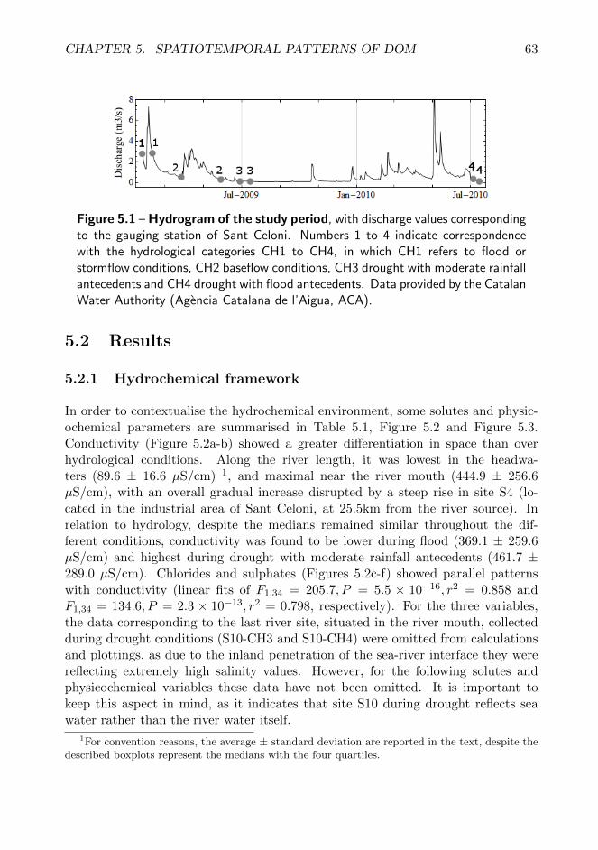
CHAPTER 5. SPATIOTEMPORAL PATTERNS OF DOM 63
Figure 5.1 – Hydrogram of the study period, with discharge values correspondingto the gauging station of Sant Celoni. Numbers 1 to 4 indicate correspondencewith the hydrological categories CH1 to CH4, in which CH1 refers to flood orstormflow conditions, CH2 baseflow conditions, CH3 drought with moderate rainfallantecedents and CH4 drought with flood antecedents. Data provided by the CatalanWater Authority (Agencia Catalana de l’Aigua, ACA).
5.2 Results
5.2.1 Hydrochemical framework
In order to contextualise the hydrochemical environment, some solutes and physic-ochemical parameters are summarised in Table 5.1, Figure 5.2 and Figure 5.3.Conductivity (Figure 5.2a-b) showed a greater differentiation in space than overhydrological conditions. Along the river length, it was lowest in the headwa-ters (89.6 ± 16.6 µS/cm) 1, and maximal near the river mouth (444.9 ± 256.6µS/cm), with an overall gradual increase disrupted by a steep rise in site S4 (lo-cated in the industrial area of Sant Celoni, at 25.5km from the river source). Inrelation to hydrology, despite the medians remained similar throughout the dif-ferent conditions, conductivity was found to be lower during flood (369.1 ± 259.6µS/cm) and highest during drought with moderate rainfall antecedents (461.7 ±289.0 µS/cm). Chlorides and sulphates (Figures 5.2c-f) showed parallel patternswith conductivity (linear fits of F1,34 = 205.7, P = 5.5 × 10⁻¹⁶, r2 = 0.858 andF1,34 = 134.6, P = 2.3 × 10⁻¹³, r2 = 0.798, respectively). For the three variables,the data corresponding to the last river site, situated in the river mouth, collectedduring drought conditions (S10-CH3 and S10-CH4) were omitted from calculationsand plottings, as due to the inland penetration of the sea-river interface they werereflecting extremely high salinity values. However, for the following solutes andphysicochemical variables these data have not been omitted. It is important tokeep this aspect in mind, as it indicates that site S10 during drought reflects seawater rather than the river water itself.
1For convention reasons, the average ± standard deviation are reported in the text, despite thedescribed boxplots represent the medians with the four quartiles.

64
pH was neutral to basic (Figure 5.2g-h). The most basic conditions were foundin baseflow (8.47 ± 0.38) and, in space, remained on average between 7.5 - 8 exceptfor sites S5, S8 and S10 which reflected peaks of higher basicity (8.37 ± 0.56 to8.91 ± 0.64). Despite a lack of data during flood, dissolved oxygen (Figure 5.2i-j) was found to be near 100% in average for the different hydrological conditions,although during drought O2% values had a higher dispersion with extreme bothhigh and low extreme values. In space, maximal averages were found again inS5, S8 and S10 (131.4 ± 48.4% to 166.4 ± 46.2 %), whereas it was minimal in S4(66.6± 26.6%).
Nitrogen in the form of nitrate and ammonium (Figures 5.3e-h) was most con-centrated in flood conditions (1.485 ± 0.656 mgN-NO–
3·L−1, 0.200 ± 0.258 mgN-
NH+4 ·L
−1); conversely, SRP (Figure 5.3i-j) was minimal under such conditions
(0.057 ± 0.041 mgSRP·L−1) and maximal during drought with flood antecedents
(0.351 ± 0.511 mgSRP·L−1). In space, SRP and N-NH+4 peak at S4 (0.633 ±
0.709 mgSRP·L−1 and 0.640 ± 0.261 mgN-NH+4 ·L
−1). Nitrate has an increasingtrend over the first three headwater sites with little temporal variability. From S4to downstream, the trend inverts and slightly decreases downstream but with animportant temporal variability. Towards the river mouth, nitrate slightly increasesagain.
5.2.2 Variation in DOM concentration
Regarding the organic solutes, DOM was quantified both in terms of DOC and DON(Table 5.2, Figure 5.3 a-d). For the whole data set, DOC ranged between 0.598 and7.873 mg·L−1, averaging at 2.758 ± 1.348 mg·L−1. DON ranged between non-detectable values and 4.272 mg·L−1, with an average of 0.565 ± 0.943 mg·L−1. Inthe headwaters were found the lowest concentrations for both DOC and DON. Then,in site S4, both solutes experience an increase. Such rise is clearer for DOC, forwhich the higher concentrations achieved in S4 remain constant downstream. In thecase of DON, sites S4 to S10 (that is, the middle and lower reaches) have a highervariability compared to the headwaters, attaining values up to 1.5 – 2 mg·L−1.However, the medians are similarly low in the middle reaches as in the headwaters,but with a higher temporal variability. In response to hydrology, DOC medianremains similar in the different conditions with higher variability during droughts.In contrast, DON differs significantly during flood (p < 0.05), exhibiting higherconcentrations and variability with respect to baseflow and drought conditions.

CHAPTER 5. SPATIOTEMPORAL PATTERNS OF DOM 65
5.2.3 Variation in DOM character
The indices considered in this study are the FI, HIX and SUVA, which reflect differ-ent and complementary attributes of DOM, namely the origin, humification degreeand aromatic degree, respectively. The three of them exhibit clearly different pat-terns in space (Figure 5.4), suggesting that they respond to different ecological andbiogeochemical processes. FI values ranged between 1.32 and 2.36 in the whole dataset. The lowest values, which indicate a terrestrial origin of DOM, are found in thethree headwater sites. Downstream, FI increases, peaking at site S7 (1.953 ± 0.270),located in the bend of Fogars de la Selva (at 45 km from source). On the otherhand, HIX has a continuous decreasing trend downstream, ranging from maximalvalues upstream (15.085 ± 2.857) until minimal values in the river mouth (7.841± 3.589). Finally, SUVA has a constant average value near 5 for the whole lengthof the river. However, the three sites in the headwaters have a higher temporalvariability compared to downstream sites.
Among the different hydrological conditions considered, different behaviours canalso be observed between these indices. For SUVA, baseflow conditions largelydiffer from the rest for exhibiting a larger variability, although it still has a similarmedian. FI in flood conditions has minimal variability and low values, whereasbaseflow and non-rainy antecedent drought have highest variability, indicating amore important heterogeneity of DOM sources along the river. HIX exhibits themost clear and significant differences (p < 0.05) in which flood conditions havehighest values and minimal variability, whereas the rest of hydrological conditionshave a higher variability.
5.2.4 Variation in DOM composition
The composition of DOM was assessed in terms of the fluorescence componentsdetermined by self-organizing map (SOM) analysis in chapter 4. As a reminder,these consist on four components, referred to as C1 to C4. Among them, C1 andC2 refer to protein-like material, and are similar to Coble’s peaks B and T, and toParlanti’s peaks γ and δ respectively. On the other hand, C3 and C4 are related tohumic-like material and can be related, respectively, to Coble’s peaks A and C andto Parlanti’s peaks α’, β, α (Coble, 1996; Parlanti et al., 2000).
Their variation in space and over time is shown in Figure 5.5. Among the fourstudied hydrological conditions, all components have in common that during floodtheir fluorescence has little variability, indicating that they remain constant alongthe river length. In the case of the protein-like components, the median is maximalduring baseflow, and minimal during flood (for C1) and during drought (for C2).In the case of the humic-like materials (C3 and C4), flood average is higher than

66
that of baseflow and similar to that of drought in the case of C4, and higher to anyother hydrological condition for C3.
Regarding space, component C3 shows no clear patterns. However, the restof components exhibit distinguishable longitudinal patterns. As for protein-likecomponents, both C1 and C2 have the trend to successively increase downstream.However, they differ in their behaviour from site S6 (located before the confluenceof the Creek of Arbucies, at 37 km from source). In this site, there is an importantdecrease in the fluorescence volume. After that, component C1 recuperates themagnitude of site S5, whereas in the case of C2, the decrease effect remains andsuccessive sampling sites remain at lower volumes, still with an increasing trenddownstream. In the case of C4, there is a monotonous decreasing pattern down-stream with a slight increase in the two last sampling sites, in the river mouth. Thisdecreasing trend of the humic-like C4 component clearly opposes to the increasingone of C1 and C2.
5.2.5 Differentiation of solutes and DOM content along the longi-tudinal gradient
A more synthetic approach on the longitudinal variation of the water chemical com-position has been addressed by computing Bray-Curtis dissimilarities of every pointof the river with respect to the first sampling site, near the river source, obtaininga profile of longitudinal differentiation downstream (Figure 5.6). They indicate towhat degree the water composition is different, or dissimilar, from site S1. Thus, aflat line would indicate a constant composition downstream, whereas higher valuesindicate a higher distance, and hence a higher differentiation, degree of a given sitewith respect to S1. These profiles have been computed for the following groups of
variables: Conservative solutes (Cl–,SO2–4 , electrical conductivity), nutrients (N-
NH+4 ,N-NO–
3,SRP), DOM concentration (DOC and DON), DOM character (FI,SUVA and HIX optical indices) and DOM composition (EEM components C1 toC4). Also, dissimilarity profiles have been computed separately for every hydrolog-ical condition.
Every type of variables exhibits a different longitudinal behaviour and sensitiv-ity to hydrology. Conservative solutes are the ones that exhibit a more consistentlongitudinal pattern for the four hydrological conditions. Both during flood, base-flow and drought they gradually differentiate from the headwaters down to the rivermouth, only altered by a steeper increase in the dissimilarity in site S4. Conversely,nutrients show a differentiated behaviour in the last half of the river length de-pending on hydrology. In the first half of the river length, nutrients compositiongradually becomes dissimilar up to site S4. From there and downstream, duringflood and baseflow dissimilarity becomes constant, indicating little change in the

CHAPTER 5. SPATIOTEMPORAL PATTERNS OF DOM 67
Figure 5.2 – Boxplot representation of the concentrations of conservative solutes in space and over
hydrological conditions. Site S1 corresponds to the headwaters whereas site S10 corresponds to the river
mouth. For the hydrological conditions, CH1 corresponds to flood, CH2 to baseflow, CH3 drought with
moderate rainfall antecedents, and CH4 drought with flood antecedents. Symbol † indicates that flood
concentrations are significantly different than the rest of hydrological conditions, whereas symbol ‡ indicates
that flood concentrations are significantly different only with respect to baseflow, both at p < 0.05.

68
Figure 5.3 – Boxplot representation of the concentrations of non-conservative solutes in space and
over hydrological conditions. Site S1 corresponds to the headwaters whereas site S10 corresponds to the
river mouth. For the hydrological conditions, CH1 corresponds to flood, CH2 to baseflow, CH3 drought
with moderate rainfall antecedents, and CH4 drought with flood antecedents. Symbol † indicates that flood
concentrations are significantly different than the rest of hydrological conditions, whereas symbol ‡ indicates
that flood concentrations are significantly different only with respect to baseflow, both at p < 0.05.

CHAPTER 5. SPATIOTEMPORAL PATTERNS OF DOM 69
Figure 5.4 – Boxplot representation of the values of DOM optical indices in space and over hydro-
logical conditions. Site S1 corresponds to the headwaters whereas site S10 corresponds to the river mouth.
For the hydrological conditions, CH1 corresponds to flood, CH2 to baseflow, CH3 drought with moderate
rainfall antecedents, and CH4 drought with flood antecedents. Symbol † indicates that flood concentrations
are significantly different than the rest of hydrological conditions, whereas symbol ‡ indicates that flood
concentrations are significantly different only with respect to baseflow, both at p < 0.05.

70
Figure 5.5 – Boxplot representation of the volumes of EEM components in space and over hydro-
logical conditions. Site S1 corresponds to the headwaters whereas site S10 corresponds to the river mouth.
For the hydrological conditions, CH1 corresponds to flood, CH2 to baseflow, CH3 drought with moderate
rainfall antecedents, and CH4 drought with flood antecedents. Symbol † indicates that flood concentrations
are significantly different than the rest of hydrological conditions, whereas symbol ‡ indicates that flood
concentrations are significantly different only with respect to baseflow, both at p < 0.05.

CHAPTER 5. SPATIOTEMPORAL PATTERNS OF DOM 71
Spatialvariability
Tempora
lvariability
CH1
CH2
CH3
CH4
S1
S2
S3
S4
S5
S6
S7
S8
S9
(*)
S10
(**)
Conductivity
Mean
369.1
437.8
461.7
389.3
89.6
104.7
129.0
516.0
490.5
446.4
620.6
575.8
686.8
444.9
µS/cm
Median
331.8
495.8
557.5
488.8
91.1
106.3
126.5
497
508.8
471.0
643.5
584.8
686.8
503.5
Std
.Dev.
259.6
247.7
289.0
239.5
16.6
17.4
20.3
187.5
124.4
74.9
153.6
70.4
68.2
256.6
n10
10
99
44
44
44
44
22
dO2
(***)
Mean
n.a.
8.763
9.592
8.924
8.392
8.922
9.168
5.770
11.240
7.917
7.693
10.688
6.310
12.865
(mg/L)
Median
n.a.
8.943
8.575
8.700
8.335
8.815
9.220
5.575
11.835
7.920
8.400
10.450
6.310
12.865
Std
.Dev.
n.a.
2.484
3.126
2.132
0.284
0.229
0.261
1.810
2.423
0.060
1.491
3.124
n.a.
2.675
nn.a.
10
10
10
44
44
44
44
13
dO2
(***)
Mean
n.a.
95.5
117.4
103.5
87.0
93.7
93.7
66.6
137.6
89.9
91.7
131.4
69.9
166.4
(%sa
t.)
Median
n.a.
90.4
97.0
93.3
89.7
94.8
93.3
66.0
142.7
92.2
97.0
117.3
69.9
160.2
Std
.Dev.
n.a.
33.3
49.1
28.5
7.6
3.3
3.1
26.6
28.4
4.0
19.2
48.4
n.a.
46.2
nn.a.
10
10
10
44
44
44
44
24
pH
Mean
7.85
8.47
8.07
8.04
7.80
7.90
7.91
7.94
8.37
7.90
7.86
8.46
88.91
Median
7.89
8.33
7.82
7.79
7.75
7.85
7.92
7.85
8.21
7.83
7.77
8.42
89.02
Std
.Dev.
0.16
0.38
0.52
0.63
0.27
0.20
0.27
0.24
0.56
0.22
0.36
0.48
0.51
0.64
n10
10
10
10
44
44
44
44
24
TM
ean
8.6
17.5
22.8
22.3
12.1
13.2
13.4
17.6
20.6
18.5
19.0
20.7
15.1
24.1
(oC)
Median
9.0
19.7
22.8
23.0
13.1
14.5
14.8
19.4
23.5
20.9
21.2
22.4
15.1
27.2
Std
.Dev.
1.5
4.5
5.3
5.0
4.6
5.3
4.5
7.1
8.1
6.5
6.8
7.9
6.8
9.9
n10
10
10
10
44
44
44
44
24
N-N
O– 3
Mean
1.485
0.845
0.690
0.564
0.299
0.589
1.071
1.339
1.023
0.922
0.835
0.840
0.997
1.232
(mg/L)
Median
1.694
0.857
0.345
0.669
0.300
0.598
1.084
1.136
0.899
0.805
0.734
0.585
0.997
1.256
Std
.Dev.
0.656
0.325
0.721
0.320
0.049
0.109
0.117
0.722
0.821
0.593
0.660
0.793
0.335
1.057
n10
10
10
10
44
44
44
44
24
N-N
H+ 4
Mean
0.200
0.042
0.166
0.132
0.022
0.028
0.025
0.640
0.212
0.111
0.092
0.051
0.046
0.075
(mg/L)
Median
0.095
0.013
0.099
0.032
0.008
0.013
0.006
0.703
0.147
0.088
0.084
0.043
0.046
0.051
Std
.Dev.
0.258
0.086
0.173
0.279
0.030
0.035
0.041
0.261
0.204
0.098
0.075
0.048
0.052
0.070
n10
10
10
10
44
44
44
44
24
SRP
Mean
0.057
0.089
0.181
0.351
0.018
0.027
0.028
0.633
0.249
0.156
0.119
0.109
0.135
0.154
(mg/L)
Median
0.062
0.102
0.116
0.180
0.009
0.020
0.023
0.417
0.187
0.119
0.107
0.093
0.135
0.154
Std
.Dev.
0.041
0.069
0.184
0.511
0.025
0.030
0.031
0.709
0.229
0.121
0.050
0.049
0.013
0.050
n10
10
10
10
44
44
44
44
24
Cl–
Mean
36.880
55.267
61.895
40.515
6.665
7.009
8.702
68.186
57.596
45.014
66.620
85.207
68.799
55.317
(mg/L)
Median
25.538
62.808
58.849
42.847
6.684
6.744
8.430
58.219
66.981
46.772
60.762
92.727
68.799
59.025
Std
.Dev.
35.887
36.489
51.442
31.105
0.808
0.996
1.438
48.309
21.603
14.523
35.434
25.624
1.573
41.031
n10
10
99
44
44
44
44
22
SO2–
4M
ean
22.408
33.281
39.270
33.191
7.445
8.324
10.592
42.294
42.913
34.126
54.274
47.380
34.948
35.181
(mg/L)
Median
24.133
39.540
41.938
38.906
7.053
8.191
10.263
38.923
47.208
36.230
55.020
51.108
34.948
39.130
Std
.Dev.
10.806
17.648
28.356
21.554
1.326
0.718
1.257
19.482
12.340
8.052
22.690
10.006
3.592
21.385
n10
10
99
44
44
44
44
22
Ta
ble
5.1
–D
ata
of
the
mea
sure
dp
hys
ico
-ch
emic
al
par
am
eter
s,su
mm
aris
edby
sam
plin
gsi
tean
dby
hyd
rolo
gica
lco
nd
iton
.

72
Spatialvariability
Tempora
lvariability
CH1
CH2
CH3
CH4
S1
S2
S3
S4
S5
S6
S7
S8
S9
(*)
S10
DOC
Mean
3.004
2.020
2.841
3.224
1.178
1.373
1.201
4.186
3.319
3.310
3.466
2.614
3.183
3.968
(mg/L)
Median
3.150
2.376
2.486
3.394
1.152
1.500
1.065
4.119
3.139
2.865
3.715
2.293
3.183
4.235
Std
.Dev.
0.986
0.874
1.579
1.716
0.435
0.323
0.436
1.476
0.480
1.188
0.776
0.785
1.167
0.993
n10
10
99
44
44
44
44
24
DON
Mean
1.322
0.458
0.148
0.593
0.148
0.164
0.309
1.191
0.646
0.632
0.611
0.437
1.243
0.610
(mg/L)
Median
1.527
0.144
0.153
0.379
0.170
0.145
0.179
1.208
0.451
0.370
0.299
0.251
1.243
0.428
Std
.Dev.
0.712
0.087
0.121
0.574
0.088
0.157
0.364
1.059
0.595
0.693
0.746
0.479
1.414
0.686
n10
10
99
44
44
44
44
24
SUVA
Mean
4.424
7.767
4.355
6.418
0.157
7.075
7.615
5.305
5.617
3.691
4.845
4.608
4.440
4.782
Median
4.446
6.050
4.385
6.581
0.364
6.772
6.278
5.474
5.519
3.879
4.352
5.091
4.440
5.046
Std
.Dev.
0.926
6.330
0.941
1.816
1.059
3.032
5.560
1.120
2.073
0.723
1.431
1.333
1.924
1.971
n10
10
99
44
44
44
44
24
FI
Mean
1.596
1.803
1.689
1.669
0.595
1.460
1.553
1.787
1.633
1.895
1.953
1.786
1.735
1.656
Median
1.628
1.801
1.583
1.640
0.693
1.468
1.550
1.822
1.636
1.849
2.008
1.798
1.735
1.627
Std
.Dev.
0.066
0.257
0.264
0.148
0.746
0.031
0.044
0.090
0.067
0.266
0.270
0.109
0.126
0.089
n10
10
99
44
44
44
44
24
HIX
Mean
13.049
6.942
10.868
9.460
12.687
15.085
11.693
7.340
7.617
12.672
8.727
7.490
9.133
7.841
Median
13.249
6.206
8.820
8.392
14.018
14.901
11.331
6.247
7.463
12.035
7.229
5.262
9.133
7.826
Std
.Dev.
1.596
2.987
5.523
3.689
4.372
2.857
2.324
2.459
2.668
3.150
4.755
4.956
6.863
3.589
n10
10
99
44
44
44
44
24
C1
Mean
9627
15864
12189
11429
9353
7567
10523
14655
14141
8996
14411
15309
14588
14621
Median
9983
16693
12952
12397
7732
7109
9522
15984
13657
8621
14141
15794
14588
13227
Std
.Dev.
1271
4145
5302
3288
3700
1523
3153
4694
3963
2546
4104
3637
5144
4335
n10
10
99
44
44
44
44
24
C2
Mean
9807
12162
11055
9841
9802
8621
11002
14859
14541
8276
9158
9460
10211
11117
Median
9807
11926
9766
8686
9223
8500
10730
15166
14424
8269
9196
9148
10211
11129
Std
.Dev.
1092
3356
3765
2301
2177
1228
2188
3617
2375
2259
640
991
1621
1187
n10
10
99
44
44
44
44
24
C3
Mean
27473
25189
25677
26662
25727
27694
26834
25669
26314
25621
26146
25199
26550
26939
Median
28323
25041
27188
26764
27583
27758
27607
26040
26097
25334
26282
26458
26550
27840
Std
.Dev.
2312
2724
3150
996
3903
716
2269
3113
1200
2252
2819
4110
2438
2638
n10
10
99
44
44
44
44
24
C4
Mean
11428
10139
11501
13004
12788
13934
17250
12230
11485
9188
8521
8043
9705
10289
Median
11350
9099
13048
13145
13117
13697
17213
12851
11262
8999
7954
7756
9705
10721
Std
.Dev.
1388
2627
3998
2407
2369
1299
1365
2973
1232
1641
2793
2088
1698
1384
n10
10
99
44
44
44
44
24
Ta
ble
5.2
–D
ata
of
the
DO
M-r
ela
ted
vari
ab
les,
sum
mar
ised
bysa
mp
ling
site
and
byh
ydro
logi
cal
con
dit
on.

CHAPTER 5. SPATIOTEMPORAL PATTERNS OF DOM 73
relative composition of ammonium, nitrate and SRP, whereas during drought theircomposition becomes gradually more similar to the headwaters, except for the finalsite which might be rater reflecting the quality of sea water instead of the river waterbecause of the inland penetration of the sea-freshwater interface. Regarding organicsolutes in terms of DOC and DON, they exhibit an intermediate profile betweenconservative and reactive inorganic solutes. In overall, there is a gradual degreeof differentiation downstream, which is greatest in site S4. But by taking a closerlook, it can also be seen that flood and baseflow have a profile which is comparableto that of conservative tracers, whereas the two droughts produce a profile whichis rather comparable with the non conservative nutrients because of the decreasingtrend after the peak in S4.
Optical variables, both the optical indices (Figure 5.6d) and EEM components(Figure 5.6e), have distinctively different longitudinal profiles. The main differenceis the lack of a consistent increase of the dissimilarity in the headwaters up to S4,observed in the three previous groups of solutes. Other than that, they reflect astrong homogenisation effect of the flooding conditions, expressed by a practicallyflat and horizontal profile. However, they also exhibit a certain degree of dissimilar-ity in the second half of the river during drought conditions. In the case of opticalindices, the dissimilarity profile increases gradually downstream, being the only casein which baseflow conditions have a distinct behaviour rather than an intermediateexpression between flood and drought. Despite these described features, the pat-terns of longitudinal differentiation for DOM quality are less clear than those of theinorganic reactive solutes.
5.2.6 Relationships between variables: a multivariate approach
The results described above provide evidence of a complex spatio-temporal rela-tionship between types of variables. In order to further relate DOM fluorescencecomposition with the surrounding hydrochemical environment, we performed a mul-tivariate statistical analysis. First, samples dissimilarities were fitted into a two-dimensional plane by computing non-metric multidimensional scaling (NMDS). Theinput variables were the EEM components C1 to C4, hence, the new ordination re-flected sample dissimilarities in terms of DOM fluorescence composition. Next, itwas tested how the rest of variables fit in this new ordination by computing a vectorfit and by assessing the significance of each one.
The computed NMDS had a correlation of R2 over 0.99 between the distances ofobjects in the obtained NMDS ordination and samples dissimilarities in the original4-dimensional space. This final ordination is shown in Figures 5.7 A and 5.7 B. Thescores of the four fluorescence components appear all at four different directions ofthe NMDS space, revealing that they are little correlated and, hence, share little

74
Figure 5.6 – Biogeochemical dissimilarity profiles of the different types of variables under
study: conservative solutes (electrical conductivity, chlorides, sulfates), non-conservative solutes
(nitrate, ammonia, soluble reactive phosphor), DOM concentration (DOC and DON), DOM char-
acter (HIX, FI and SUVA) and DOM composition (fluorescence components C1 to C4).
information. In overall, sample and variable scores are more widely dispersed overthe first axis. In the positive side there are the two protein-like variables (C1 andC2), whereas in the negative side we find the humic-like ones (C3 and C4). Hencethe first axis divides our samples according to the relevance of either protein-likeof humic-like moieties. Besides, the second axis further differentiates between thetwo protein-like components, as C1 is oriented in the negative part, and C2 in thepositive part. This suggests that the two components, despite having a similarcomposition, may be driven by different processes and sources.
For the sake of facilitating the interpretation of the samples distribution on theNMDS plane, samples have been grouped by sampling site Figure 5.7 A, reflectingthe spatial extent; and by hydrological conditions Figure 5.7 B, reflecting the tem-poral extent. It should be noted there that both figures correspond to the sameNMDS compoutation and only the visualisation and grouping of the samples dif-fers. Regarding Figure 5.7 A, corresponding to the spatial extent, the location of

CHAPTER 5. SPATIOTEMPORAL PATTERNS OF DOM 75
the centroids for the different sampling sites clearly reflects three different groups.On the negative side of the first axis appear the headwater sites S1 to S3, as wellas site S6 little distance apart. They appear at the direction of the fluorescencecomponents C3 and C4, indicating the predominance of humic-like DOM materi-als. On the other hand, the sites of the last part of the river (S7 to S10) appearin the positive side of the first axis, directed toward the fluorescence componentC1. Finally, sites S4 and S5 appear at the positive side of the second axis, at thesame direction as the fluorescence component C2. This indicates that C2 is moredirectly related to anthropogenic DOM sources, whereas C1 could be more directlyattributed to in-stream DOM processes.
A series of hydrochemical variables have been fitted in to the NMDS ordinationby means of a vector fitting analysis. Those whose fit had a significance of p <0.05, have been added to the NMDS plot. Interestingly, they appear directed tothe three directions described above for the sampling sites centroids. HIX appearsat the direction of the headwater sites, FI together with the conservative solutes(Conductivity, chloride and sulphate) appear with the lowland river sites, and fi-nally, DOC, ammonia and SRP appear with sites S4 and S5. Also, it is noteworthythat two variables directly related to DOM held no significance (DON and SUVA),as well as nitrate.
On the other hand, in Figure 5.7 B sample centroids reflect the hydrologicalextent. The confidence interval circle around the centroid indicates the dispersiondegree of the samples of every hydrological condition throughout the NMDS plot.Out of that, it can be observed that during flood the samples are minimally dis-persed, indicating little dissimilarities between them. During baseflow and drought,the dispersion gradually increases. Whereas the dispersion degree is similar forbaseflow and drought with wet antecedents, it becomes maximal during droughtwith dry antecedents. Despite this difference between the two droughts in the dis-persion degree, they remain similar in the position of the centroid, which indicatessimilar qualitative DOM trends. The centroids are located near the axes originand the dispersion occurs throughout the whole plane. This indicates that duringdrought, both humic-like and protein-like DOM substances are present along theriver length. However, in flood and baseflow the samples appear distributed at somespecific sectors of the NMDS space. Flood is located in the negative first axis, indi-cating the prevalence of humic-like and humified DOM substances throughout theriver. By contrast, baseflow samples are mainly located in the positive first axes,hence indicating a predominance of protein-like substances of microbial origin.

76
Figure 5.7 – NMDS ordination based DOM on compositional dissimilarities. Gray labels
represent the fluorescence components scores, and black arrows, the chemical variables significantly
fitted in the ordination (p < 0.05). These are only plotted in panel A, but are equivalent for panel
B. A) Samples are grouped by sampling site and represented by their centroid. B) Samples are
grouped by hydrological conditions. Ellipses around centroids represent confidence areas of the
samples dispersion (confidence limit se = 0.95)

CHAPTER 5. SPATIOTEMPORAL PATTERNS OF DOM 77
5.3 Discussion
5.3.1 Spatio-temporal patterns of inorganic and organic solutes
The water chemistry of La Tordera exhibits some characteristic features along theriver length. One clear differentiation are the first three sampling sites, that aresituated in the headwaters, from the river source until the village of Santa Maria dePalautordera (sites S1 to S3). These sites are characterised by low concentrationsof all measured anions with a small seasonal variability, including both conservativeand non-conservative anions. This reflects the low relevance of anthropogenic efflu-ents, as well as a low weathering of the siliceous geological substrate in that part ofthe river (Mas-Pla et al., 2012).
Next to that, the river runs through the urban and industrial area of SantCeloni. In this part of the river lies the sampling site S4, which exhibits a drasticchange of the chemism. This change mainly corresponds to an increase of theconcentrations of the conservative tracers of chloride, sulphate and conductivity, aswell as the nutrients of N-NH+
4 , SRP and DOC, together with N-NO–3 and DON
to a certain extent. This increase remains downstream and even further augmentsin the case of the conservative anions. However, the rest experiment a depletiondownstream, even if the influence of human activity is still present throughout sitesS5 and S6. This uncoupling between the conservative and the non-conservativesolutes evidences the presence of bioreactive processes that are responsible for theavailability of these solutes. Some of these nutrients recuperate basal concentrationsrapidly after site S4 (N-NH+
4 , SRP), while some others do it more moderately (N-
NO–3 and DON). Interestingly, DOC concentration never recuperates headwater
levels, suggesting a lower bioreactive character with respect to the nitrogenatedsolutes. These evidences of the presence of relevant reactive processes, as wellas the presence of confluences with little or non-impacted tributaries, have beenpreviously described as attenuators of the anthropogenic pressure that operates inthis central part of the river (Mas-Pla et al., 2012).
Over the different hydrological conditions assessed in this work, the longitudi-nal dissimilarity profiles for all the mentioned solutes provide evidence of a higherdegree of biological reactivity in drought conditions with respect to flood conditions(Figure 5.6). This seasonality is clearer for inorganic than for the organic solutes(compare Figure 5.6b vs 5.6c), hence reflecting a major dependence of the bioreac-tive character of DOC and DON (and therefore, of DOM concentration) with thehydrological conditions.
Regarding the export capacity of the different solutes, floods are the the hydro-logical conditions that are more efficient especially for the nitrogenated solutes andSRP. Among them, the most accentuated difference between stormflow and the rest

78
of hydrological conditions occurs with DON. Pulse flood events have been found tocommonly produce [DON]pulse:[DON]baseflow > 1. For Mediterranean rivers with-out reservoirs (Martin and Harrison, 2011) determined a [DON]pulse:[DON]baseflowratio of 1.45 from average concentrations of 0.220 and 0.151 mgDON·L−1 duringflood and baseflow conditions, respectively. In the present study, this ratio is ex-ceeded by far (up to 10.6), and even exceeds the highest ratio reported in Martinand Harrison (2011), which is 2.22 for temperate river systems. While our averagesin baseflow and drought are similar to those reported by them, our flood averageis much higher (1.322 ± 0.712), which causes the ratio to increase so much. Theseresults highlight the high potential of La Tordera to export nitrogen in dissolvedorganic form following flood pulses. While point sources are unlikely to be the ori-gin of such export, because they would have become diluted by the high flows, theymay be attributable to a flushing effect reflecting the characteristics of the catch-ment being drained, i.e. catchment land uses. Evidences in this sense can be foundfor instance in Lorite-Herrera et al. (2009), who reported high DON concentrations(ranging between 6.3 and 19.8 mg·L−1) and annual exports in an agricultural catch-ment, which were one order of magnitude higher than those from similar pristinesystems. This excess was attributed to the leaching and drainage of organic nitrogenfrom agricultural soils.
In contrast to DON, DOC did not show any significant differences between hy-drological conditions. Positive and strong correlations between DOC and dischargehave been widely reported, and usually even more consistently than for DON (Clairand Ehrman, 1996). As in this study we are comparing means that include samplesfrom the whole length of the river, spatial complexity and variability may be blur-ring the usually clear relationship between DOC and discharge. Indeed, statisticallysignificant differences in space were found for DOC and not for DON.
5.3.2 Spatial trends of DOM quality
Unlike for the solutes concentrations, less clear patterns can be observed out of theboxplots in space and over hydrological conditions for the qualitative DOM variables(Figures 5.5 and 5.4). However, a multidimensional approach with an NMDS anal-ysis was useful to elucidate associations between samples and qualitative variablesand, also, to unveil interesting longitudinal patterns and hydrological influences.Indeed, the ordination of the samples in a two-dimensional space based on compo-sitional dissimilarities showed a clear segregation of sampling sites into three maingroups: one including sites from the headwaters until the middle reaches, anotherone representing the lowland part of the river, and finally, another one including thesites S4 and S5, situated downstream the anthropogenically impacted area of SantCeloni. Moreover, the significant fit of optical indices provided more consistency

CHAPTER 5. SPATIOTEMPORAL PATTERNS OF DOM 79
to this spatial differentiation based on DOM quality. Hence, it becomes clear thatDOM undergoes a compositional change as it is being transported downstream.
The headwater sites S1 to S3 are related to components C3 and C4, as well asto the optical index HIX. This provides evidence that the DOM flowing in this partof the river has a predominantly humic-like nature of terrestrial origin. This is asexpected, as these sites are located in a mountainous, forested area with minimalanthropogenic perturbation. In similar systems, EEMs have been reported to pro-duce A-C shapes (equivalent to our C3 and C4 components) with high aromaticcharacter (Hudson et al., 2007; Fellman et al., 2010).
Next, sites S4 and S5, appear differentiated in the NMDS as being related toa DOM with tryptophan-like nature (C2), as well as with the presence of nutri-
ents (SRP, N-NH+4 and DOC). This differentiation in terms of DOM composition
is consistent with previous findings where sewage inputs appeared to release DOMwith distinguishable fluorescence signatures with respect to natural riverine DOM(Baker, 2001; Spencer et al., 2007; Henderson et al., 2009) mainly due to intensemicrobial transformations (Park et al., 2010). Peak T, equivalent to our C2 com-ponent, has been even used as a tracer of anthropogenic inputs (Baker, 2002).
After these two sites, the impact of the waste water treatment plant (WWTP) isno longer evident, and site S6 appears near the headwater sites. This rapid shift inthe DOM composition can be due, to the one hand, to the inputs of water from nonor less polluted tributaries (Fuirosos, Breda, Arbucies) which may have diluted theupstream DOM quality. On the other hand, protein-like components are consideredto be one of the most labile fractions of DOM (but see Cory and Kaplan (2012)),hence the biological uptake of these moieties may have further favoured the depletionof the C2 component. This sounds reasonable at the reaches near site S6, as theriver morphology has already become more shallow with increased water residencetimes and open canopy which facilitate the biophysical opportunities for in-streamDOM processing (Battin et al., 2008). Also, this is in consonance with our evidencesof biological retention processes in the second half of the river, described above outof the dissimilarity profiles (Figure 5.6). Another factor that may influence suchminimisation of the anthropogenic inputs can be a dilution effect coming from ageological fault that creates an effluence of groundwater with little mineralisationfew kilometres upstream of site S6 (named Gorg de Perxistor, described by Mas-Plaand Mencio (2008)).
Finally, after the bend of Fogars de la Selva until the river mouth, the natureof DOM exhibits another shift. In this case, its composition is mainly related toC1 component, a fluorescence signal similar to that of tyrosine-like components. Itrepresents a protein-like material, different than that observed for S4 and S5, whichcorrelates with FI. This further suggests an in-stream origin of the DOM for thelast part of the river. As in site S6, the persistence of a shallow and open canopy

80
characteristics, as well as because of the lack of significant tributary inputs, mayexplain the proliferation of an in-stream DOM production by algae and microbialactivity.
5.3.3 Influence of hydrology on the determination of spatial trends
Among the different hydrological conditions sampled in this study, floods representthe conditions in which the maximal spatial homogeneity of DOM character is ob-served. Under these circumstances, DOM samples appear aggregated in the NMDSplane, suggesting that hardly any qualitative changes occur during the longitudi-nal transport. Instead, samples from low flow dates (CH3 and CH4) appear moredisperse, suggesting a high heterogeneity of DOM properties.
Under flood conditions, the location of the centroid in the positive first axis ofthe NMDS indicates a strong predominance of humic-like substances of terrestrialorigin. This allochthonous input of DOM in the river water during storms has beenespecially documented for forested catchments (Raymond and Saiers, 2010). Duringstorms, hydrological flow paths shift to more superficial soil horizons richer in DOMwhich has been accumulated during the low flow periods (Sanderman et al., 2009).This DOM is rapidly flushed out to the riverine channel, resulting in an increaseof DOM concentration (Hinton et al., 1997; Mulholland, 2003) and in a qualitativeshift to vascular plant-derived humic substances (Hood et al., 2006; Fellman et al.,2009b; Nguyen et al., 2010). This flushing behaviour for DOM has already beendocumented for the basin of Fuirosos, one of the tributaries of the present study site(Butturini et al., 2008). Fuirosos has a completely forested land cover. In contrast,the catchment of La Tordera has a variety of land uses. Forests are distributedmainly in the upland Montseny Massif and in the Montnegre slopes whereas otherland uses including agriculture and urbanisation are found in the lowland. Thedrainage of these areas has been found to produce a differentiated fluorescencesignal in comparison to forested catchments, reflecting the inputs of labile and lowhumified DOM (Wilson and Xenopoulos, 2009; Williams et al., 2010). However, thissignal does not appear to influence in a relevant way the samples collected duringflood conditions. It has been reported that the export of DOM from crops andurban areas is primarily driven by the anthropogenic activity rather than by localrainfall events (Duan et al., 2007). Therefore, we suggest that during storms forestedareas are those with the highest potential to export DOM to the river. Consequentlyduring stormflow riverine DOM reflects mainly a terrestrial source and this characterremains similar along the entire main stem, suggesting a conservative transport.
Surprisingly, this persistance of an humic-like character during flood co-occurswith a high increase of DON concentration (Figure 5.3d). This coexistence seems todiscard the option that the exported DON be in the form of protein-like substances.

CHAPTER 5. SPATIOTEMPORAL PATTERNS OF DOM 81
Rather than that, it may be part of the humic-like fraction, or just not be part ofthe optical fraction of DOM and hence, not reflected in the EEM components.
However, as soon as rainfall decreases in frequency and in intensity, the domi-nance of the DOM terrestrial character observed during flood gives way to a longi-tudinal differentiation of DOM fluorescence properties. During the drying process,not only does discharge decrease, but also change the flowpaths which feed the river(Hinton et al., 1998) and the connection between the river and the terrestrial catch-ment becomes weaker. The drainage of DOM-rich subsurface soil horizons graduallyceases and the river surface water is mainly sustained by deep groundwater whichis poor in DOM. Therefore, drought minimizes the terrestrial sources of riverineDOM, which only remain in the headwater sites (S1-S3). Downstream, samplesappear associated to the presence of protein-like substances, either resulting fromanthropogenic or in-stream sources.
During low flows the river loses dilution capacity and, therefore, any inputs suchas natural tributaries or WWTP effluents have a major impact on the propertiesof the bulk DOM of the main stem. On the other hand, as flows decrease theconnectivity between river reaches diminishes and appear retention areas wherewater residence times are high. These areas constitute sections of the river channelwhich increase the microbial opportunities for DOM in-stream processing (Battinet al., 2008), as well as for autotrophic DOM production (Peduzzi et al., 2008). Thusin overall, drought maximises the variety of processes that can potentially modifythe bulk DOM pool, and these processes vary along the main stem due to the varietyof land uses, anthropogenic influence, and geomorphologic features in the catchment(Jaffe et al., 2008). Therefore during dry conditions the local characteristics andenvironmental conditions of each riverine reach become the primary drivers of bulkDOM properties, and this results in a spatial mosaic of varied DOM fluorescentsignatures. Also, our results suggest that the hydrological antecedents regulate themagnitude of such spatial differences, where longer previous dry periods contributeto amplify the longitudinal heterogeneity of DOM character.
5.3.4 Next steps: Transport vs Reaction, integrating informationfrom the tributaries
Between the contrasted hydrological conditions of flood and drought, baseflow showsan intermediate degree of dispersion in the NMDS plot, and appears clearly differ-entiated from flood by being centred at the negative first axis, near to the directionof the C1 component and FI. This sharp segregation between the samples of floodand baseflow conditions shows a clear differentiation of DOM quality as soon as thestormflow ceases. This shift from humic-like to protein-like substances, as well as tothe shift from terrestrial to in-stream DOM sources suggests that as soon as storm-
82
flows cease, in-stream processes start to operate and to structure a longitudinalpattern of DOM quality.
Hence, this chapter suggests that lower flows increase the chances for DOMin-stream processing and favour a higher spatial variability of DOM quality andquantity. However, with the sampling design used in this study the relevance ofin-stream reactivity over downstream transport cannot be demonstrated. Alongthe main stem, and especially along the middle reaches, La Tordera receives thewaters of numerous tributaries draining a variety of land uses, as well as a numberof anthropogenic point sources whose dynamics respond more to socio-economic as-pects rather than hydro-climatic. Therefore, the higher spatial variability observedduring low flows could be due to the fact that the river has a lower dilution capacityof these inputs and tributaries that join the main stem successively downstream.
Because of that, in order to take a step further and assess the relevance of in-stream processing in shaping the longitudinal patterns of DOM quality and quantity,the longitudinal sampling design used in this study should be complemented withcomprehensive information about the waters that the main stem receives along itslength.
5.4 Conclusions
The results of this study highlight the importance of hydrology and space in thedetermination of DOM quantity and quality:
• Along the main stem, the river exhibits three reaches with a consistent dif-ferentiated DOM character: the headwaters, the region near the town of SantCeloni, and the low part of the river flowing between the bend of Fogars de laSelva and the river mouth.
• In the headwaters, DOM has an eminent humic-like character coming from thedrainage of the surrounding terrestrial catchment. During flood conditions,this character remains downstream.
• Near Sant Celoni, there is a shift in the DOM quality, expressed as a pre-dominance in the protein-like component C2. A concomitant increase in thechlorides and nutrients content of the water suggests that this shift in theDOM quality is caused by the direct outlets of a WWTP and possibly otherindustries in the beginning of the river reach.
• In the lower part of the river, high water residence times and light availabil-ity favour the conditions for in-stream DOM production and transformation,

CHAPTER 5. SPATIOTEMPORAL PATTERNS OF DOM 83
which results in an increased FI and predominance of the protein-like EEMcomponent C1.
• Whereas flood conditions induce an homogenisation of the DOM characterover the longitudinal dimension, baseflow and drought favour spatial differen-tiation resulting from the influence of the local characteristics of the river atevery reach.
• The hydrological antecedents of a drought period determine the magnitude ofthe spatial differentiation of DOM character. A longer previous dry periodcontributed to an amplification of the longitudinal differentiation.
• This suggests a seasonal role of the river with respect to DOM, shifting be-tween transporter and transformer. Such alternation in the transport andprocessing of DOM can have further implications for the understanding of thecarbon cycling at higher scales, and may contribute to the ongoing debate onthe role of inland waters on the global carbon cycle.

84

Chapter 6
Multivariate exploration ofDOM quality and reactivity inthe main stem of La Tordera
6.1 Introduction
In the previous chapter, a longitudinal assessment of dissolved organic matter(DOM) quality revealed that, at low discharge conditions, there was an emergenceof spatial heterogeneity in DOM quantity, fluorescence composition and character.The Fluorescence Index (FI) suggested that in-stream processes could be favouringsuch spatial heterogeneity, especially in the lower reaches of the river. However, thesampling design did not take into account the quality of the tributaries joining themain stem. Hence, it could not be concluded whether such longitudinal changeswere effectively the result of in-stream processes, or on the contrary, the result ofthe physical mixing with the waters of the tributaries, inputting a diversity of DOMcompositions and character.
In order to provide more evidences about the relevance of DOM in-stream pro-cessing over transport, in this chapter we use coupled data from the main stem,as well as from the tributaries that originate the water and solutes flow of themain stem. With the use of an end-member mixing analysis (EMMA) approach,we explore to what extent the DOM composition observed in the main stem canbe attributed to the physical mixing of the tributaries or, by contrast, whether itresponds to biogeochemical interactions during its downstream transport.
Multivariate ordinations have been widely used to study water mixing processesin catchments since the seminal papers of Hooper et al. (1990) and Christophersen
85

86
and Hooper (1992). Its most common use has been to identify the water sources incatchments (Hooper, 2001) or groundwater systems (Long and Valder, 2011), hencethe ordination is based on conservative tracers (Christophersen and Hooper, 1992),and their main challenge is to identify the adequate number of end-members thatcan effectively explain the water sources within the system. That is, conservativetransport is assumed, and the unknown are the water sources (Barthold et al., 2011;Valder et al., 2012). Here, we use an alternative approach in which the reasoning isthe opposite: the sources are well-known (i.e. the tributaries) and the conservativeversus non-conservative transport is tested.
For this assessment, six additional surveys were performed in which the tribu-taries and anthropogenic outlets discharging at the main stem were comprehensivelysampled. These water inputs effectively represented the solutes and water flux alongthe main stem, as it is later shown in Chapter 7. Also, the sampling effort in themain stem was intensified especially in the middle reaches, where the confluencesare most frequent. These six additional surveys were conducted between July 2011and March 2013, and were sought to span a range of hydrological conditions. Inthis case, we captured an extreme flood event of 156 m3/s, which was four orders ofmagnitude higher than the lowest flows conditions, of 0.065 m3/s. Between thesetwo hydrological extremes, we sampled baseflow (3.10, 1.90 and 1.532 m3/s) anddrought (0.47 m3/s) conditions (see section 3.2.2 for further details on the sam-pling strategy). These surveys, added to the longitudinal ones, created altogethera data set of 270 samples, including a longitudinal gradient, a variety of tributariesand anthropogenic outlets, as well as a range of hydrological conditions. This largedata set provided the opportunity to better explore spatio-temporal patterns ofDOM quality in La Tordera, as well as relationships between chemical and opticalparameters.
According to that, the main objectives of this chapter were two-fold:
1. To explore spatio-temporal variation in the DOM composition, and the rela-tionships between the fluorescence components and other optical and chemicalvariables.
2. To evaluate to what extent the DOM composition observed in the main stemcan be explained as solely the physical mixing of input tributaries or, bycontrast, whether in-stream processing may be operating.
To address these aims, we performed a fluorescence composition-based non-metric multidimensional scaling (NMDS) analysis with the whole 270-samples dataset. This analysis a) was complemented with a vector fit analysis to attain objective1, and b) was used to create mixing diagrams to address objective 2, as in Christo-phersen and Hooper (1992): Based on the EMMA approach, we follow the rationale

CHAPTER 6. MULTIVARIATE EXPLORATION OF DOM REACTIVITY 87
that if the water composition in the main stem is only the physical mixing of thetributaries, then the main stem samples will lie within the polygon formed by thetributaries in the NMDS ordination.
6.2 Results
6.2.1 Characteristics of the tributaries
The most concentrated inputs of DOM to the main stem of La Tordera correspondedto two industrial effluents (Industry 1 corresponding to site A4 and Industry 2corresponding to site A8 as shown in Figure 3.5) and the creek of Reixac. Theindustries represent direct inputs of anthropogenic waters, whereas the creek ofReixac represents a semi-direct input, as it receives the effluents from a waste watertreatment plant (WWTP) just some few meters before the confluence with the mainstem. The effluent of Industry 1, situated in the industrial area of Sant Celoni, hadthe highest average dissolved organic carbon (DOC) concentration, consisting of43.13 ± 14.19 mg L−1, ranging between 29.86 and 67.6 mg L−1. The effluentof Industry 2, situated in the industrial area of Hostalric, introduced DOC at anaverage concentration of 18.94 ± 19.39, ranging between 1.89 and 46.64 mg L−1.The creek of Reixac, situated in the lower part of the river (at 53 km from the riversource, and at 8 km to the river mouth) had an average DOC concentration of 13.14± 9.55 mg L−1, ranging between 3.46 and 24.11 mg L−1. All these three inputs hada median DOC concentration (38.72, 13.61 and 12.49, respectively) over the generalone (4.46 mg L−1). Regarding dissolved organic nitrogen (DON) concentrations,the same trend could be observed, so that Industry1, Industry2 and the creek ofReixac had a higher median DON concentration than the general one. Again, themost notable DON input was found for Industry 1, which had an average DONconcentration of 4.40 ± 4.80, ranging between 0 and 10.94 mg L−1. Industry 2 andthe creek of Reixac had lower average DON concentrations (0.91 ± 0.82, rangingbetween 0 and 1.75 mg L−1; and 1.62 ± 1.92 mg L−1, ranging between 1.92 and4.49, respectively), although their median (0.95 and 0.80 mg L−1, respectively) wasstill higher than the overall one (0.221 mg L−1).
For the fluorescence components, it could also be observed that anthropogenicwaters had higher intensities than the natural tributaries with little impact, al-though the differences were not as pronounced as for the quantitative parametersof DOC and DON. For the protein-like fluorescence represented by component C2,the inputs which had a higher median than the overall one (11522 r.u.3 nm−2)were the WWTP of Santa Maria de Palautordera, the creek of Pertegas, Industry1and the creek of Reixac (whose means were, respectively, 26884, 21258, 31737 and31477 r.u.3 nm−2). The WWTP of Santa Maria de Palautordera are direct inputs

88
of anthropogenic waters, whereas the creeks of Pertegas and Reixac are semi-directinputs, as they receive the waters of a WWTP just some few meters before theirconfluence with the main stem of La Tordera. The same effluents also had a highermedian humic-like fluorescence compared to the overall one, which was of 14390r.u.3 nm−2. The medians of the WWTP of Santa Maria de Palautordera, the creekof Pertegas, Industry1 and the creek of Reixac were, respectively, of 26884, 21258,31737 and 31477 r.u.3 nm−2, respectively.
6.2.2 Fluorescence composition-based NMDS ordination
Characteristics of the ordination: Variable loadings and vector fittinganalysis
The NMDS analysis fitted the original four-dimensional space (defined by the fourfluorescence components) into two dimensions with a high goodness of fit (non-metric fit R2=0.997; linear fit R2=0.988). As it can be seen in Figures 6.3 and 6.4the first axis separates the humic-like components C3 and C4 (negative side) fromthe protein-like components C1 and C2 (positive side).
The results of the vector fitting analysis are overlaid as white labels. Humifica-tion Index (HIX) is oriented to the negative side of the first axis, whereas FI andBiological Index (BIX) appear towards the positive direction of the first axis, allwith a high level of significance (p < 0.001, except Specific Ultra-Violet Absorbance(SUVA) for which p < 0.05). This reinforces the interpretation of the components,so that C1 and C2 are related to autochthonously derived components, whereas C3and C4 are related to terrestrially-derived components.
The secondary axis separates C1 and C3 from C2 and C4, suggesting furtherdifferentiation within the protein- and the humic-like groups of components. SUVAappears directed towards the negative secondary axis and C3 (p < 0.05). It is note-worthy, though, that SUVA and HIX appear perpendicular, showing independencefrom one another. A series of chemical solutes, such as DOC, total nitrogen (TN),ammonium and soluble reactive phosphor (SRP) were significantly (p < 0.01) ori-ented to the positive side of the second axis, near C2. This indicates that samplesappearing at that direction may be related to nutrient-enriched sites. On the otherhand, the chemical solutes with the most conservative behaviour (nitrate, chloride,sulfate and electrical conductivity), did not fit significantly (p > 0.05) to the fluo-rescence DOM-based NMDS ordination.

CHAPTER 6. MULTIVARIATE EXPLORATION OF DOM REACTIVITY 89
Figure 6.1 – DOC and DON inputs from the tributaries. The top axis indicateswhether the inputs refer to D=direct or SD=semi-direct inputs of anthropogeniceffluents. The horizontal line corresponds to the overall mean.

90
Figure 6.2 – Humic-like and protein-like inputs from the tributaries. The topaxis indicates whether the inputs refer to D=direct or SD=semi-direct inputs ofanthropogenic effluents. The horizontal line corresponds to the overall mean.

CHAPTER 6. MULTIVARIATE EXPLORATION OF DOM REACTIVITY 91
Figure 6.3 – NMDS showing the ordination of the end-members. NMDSanalysis, in which only the tributaries and anthropogenic outlets have been plotted.Sites have been coloured to distinguish between natural tribuaties, WWTPs andindustries. The polygon outlines the mixing domain defined by all the tributaries(i.e. end-members).
Tributaries as end-members of DOM composition in the main stem
Figure 6.3 shows the tributary sites, which comprise a mixture of natural and an-thropogenic water types. The samples corresponding to natural tributaries withminimal anthropogenic impact (riverine category) appear spread over the wholeNMDS plane, occupying the space of both sides of the primary and secondary axes.However, industrial effluents appear only in the positive side of the secondary axis.As for WWTP effluents, they show a very clear relationship with the fluorescencecompnent C2, suggesting a relationship between C2 and sewage-derived DOM.
Altogether, they delineate a polygon region hereafter referred to as endmemberpolygon. This polygon disginguishes between two regions: the inner region containssamples which can be potentially due to the physical mixing of the waters fromthe tributaries; and the outer regions, where the composition of the samples cannotbe explained solely by the tributaries and, hence, is indicative of the presence ofin-stream processing deriving such compositional changes.

92
Figure 6.4 – NMDS showing the ordination of the main stem sites. NMDS
plot in which only the main stem sites have been plotted and coloured according to their river
reach (A), and the hydrological conditions under which they were sampled (B). In panel A, space
categories correspond to Headwaters (0 to 20 km from source), middle reaches (20 to 40 km) and
lowland (40 to 60 km, i.e. river mouth). In panel B, hydrology categories correspond to flood
(> 4m3/s), baseflow (4 to 1 m3/s) and drought (< 1m3/s) – Discharge measured in Fogars de
la Selva.

CHAPTER 6. MULTIVARIATE EXPLORATION OF DOM REACTIVITY 93
Ordination patterns due to hydrology and space
In order to explore spatio-temporal patterns of DOM composition in the main stem,Figure 6.4 shows only the main stem sites, as well as the endmember polygon derivedin the previous section.
In space (panel A), the most important segregation occurs on the second axis.The sites from the lowland appear on the negative side, whereas those from theheadwaters and the middle reaches are found on the positive side. Furthermore,headwater samples appear slightly more concentrated in the region between C3 andC4, similarly to the situation for flood samples in panel B. In relation to the vectorfitting analysis, the headwater samples are mainly related to HIX, the sites from themiddle reaches to the chemical nutrients and Spectral Ratio (SR), and the lowlandsites with the indices BIX and FI, as well as with SUVA and Spectral slope (S). Itis noteworthy that all the samples that appear outside of the polygon formed bythe tributaries correspond to sites of the lowland.
In panel B, objects are coloured according to the discharge category under whichthey were sampled. The samples collected during flood conditions appear clearlyaligned between the region of C3 and C4. Samples from baseflow and drought condi-tions appear more broadly distributed throughout the whole NMDS plane. Droughtsamples seem to be more dispersed and, together with some baseflow samples, oc-cupy the negative secondary axis outside the polygon formed by the tributaries.
6.2.3 Mixing diagrams at a range of hydrological conditions
In order to explore the relevance of in-stream processing over transport, mixingdiagrams have been build for those surveys with data about the tributary inputs(Figure 6.5). From the whole NMDS analysis, only the samples from every spe-cific survey have been plotted in each panel, with their corresponding endmemberpolygon.
During the flood survey, all the main stem samples appear aggregated inside theendmember polygon, at the negative side of the primary axis. This suggests thatthe DOM composition in the main stem is the result of the physical mixing of somefew tributaries, and that those located at the positive side of the primary axis donot have much impact on the final composition in the main stem.
However, in the rest of hydrological conditions, an important number of sampleslie in the outer region of the endmember polygon. Lowland sites appear practicallyalways outside the polygon, however, samples from the middle reaches and evenfrom the headwaters can also be found in this outer region, i.e. panels C, D and F.

94
Figure 6.5 – Mixing diagrams at a range of hydrological conditions, derivedfrom the NMDS ordination. The discharge stated in the plot labels was recordedin Fogars de la Selva. (*) In the survey of 1.53 m3/s only the middle reaches weresampled.

CHAPTER 6. MULTIVARIATE EXPLORATION OF DOM REACTIVITY 95
6.3 Discussion
The characteristics of the NMDS ordination perfomed on the complete data setyielded very similar results as the NMDS analysis performed only on the longitudi-nal samplings (previous chapter). However, here we improved the spatio-temporalresolution, hence obtaining more robust results; and most importantly, we gainedthe information provided by the tributaries, which revealed the presence of somesamples whose composition could not be the result of the physical mixing of thetributaries but, on the contrary, had to be the result of in-stream processing.
6.3.1 Spatio-temporal patterns of DOM composition in the mainstem
The NMDS analysis performed in this chapter reinforced the evidences that floodconditions homogenise DOM composition along the whole river length. During suchextreme high flows, DOM composition consisted of a high prevalence of humic-like substances, defined by components C3 and C4, and its bulk properties werecharacterised by a high humification degree. This demonstrates a strong connectionof the riverine DOM with the terrestrial catchment, typical of stormflow events inforested catchments (Vidon et al., 2008; Nguyen et al., 2010). However, out of floodconditions, there was a clear segregation of samples according to their longitudinaldistribution along the main stem (Figure 6.4).
Headwater sites appeared clustered with the samples collected during flood, sug-gesting that during such high flows, DOM composition of headwater sites remainedconstant along the whole length of the river. The middle reaches appeared mainlyaccumulated in the positive secondary axis, spanning the space between C4 and C2loadings, and towards the direction of the nutrients from the vector fitting analysis.If we consider the finding that C2 is directly related to WWTP outlets (Figure 6.3),then it follows that the middle reach sites exhibit a gradual shift in its compositionfrom a predominance of C4 – characteristic of the headwaters –, to a predominanceof C2 – indicator of sewage water. The relationship with nutrients provided by thevector fitting analysis reflects the fact that the main tributaries discharge to themain stem in these middle reaches. Most of these tributaries flow along importanttowns and receive the waters of a number of industries and WWTPs. For instance,the creek of Arbucies receives the waters of the WWTP of Arbucies in the headwa-ters, and those of the WWTP of Hostalric in its lower part, right before dischargingto La Tordera. Similarly, the creek of Breda receives first the outlet of the WWTPof Breda and then that of the WWTP of Riells i Viabrea. The creek of Gualbareceives the waters of the WWTP of Gualba in its middle reaches, and the creek ofPertegas receives the waters from the WWTP of Sant Celoni a few meters before

96
its confluence with La Tordera. Finally, Vallgorguina receives the outlets of theWWTPs of the towns of Vallgorguina and Vilalba Sasserra. Therefore when theyreach the main stem they are nutrient enriched (Mas-Pla and Mencio, 2008).
Finally, the lowland sites appear separated on their own, but dispersedly dis-tributed at the same time, in the area of the negative secondary axis. There,samples appear between the loadings of C3 and C1, hence also exhibiting a rangebetween humic-like and protein-like components, but different from those in themiddle reaches. Here, C1 appears to be closely related with high values of BIX andFI, therefore indicating that C1 is the result of in-stream biological activity (McK-night et al., 2001; Huguet et al., 2009). The distance between C1 and the DONendmembers would suggest that, whereas C2 may reflect protein-like componentsof anthropogenic origin, C1 may be indicator of protein-like components generatedin-stream. This would be in line with evidences of non-conservative DOM transportalong these lowland sites.
BIX, FI and HIX exhibited a consistent behaviour according to the predominantinterpretation of these indices in the literature (Fellman et al., 2010). BIX andFI, as indicators of an in-stream origin of DOM, were related to the protein-likecomponent C1 as well as to lowland sites were non-conservative transport has beenfound to be predominant. On the other hand, HIX is inversely related to BIX andFI, as it indicates the presence of highly humified humic substances, here relatedwith headwater sites and flood periods when the water DOM reflects the terrestrialdrainage of the catchment.
But, more surprisingly, HIX and SUVA vectors appeared at perpendicular direc-tions, showing little relationship between DOM humification degree and aromaticity.Both aspects (humification and aromaticity) have been found to be linked in a num-ber of organic materials (Fuentes et al., 2006); therefore, HIX and SUVA would beexpected to covary. However, both indices have been found to provide uncoupledresults when compared one another (Singh et al., 2014). Such inconsistencies mayarise from the fact that as both indices are obtained with different methods (fluo-rescence and absorbance) they may be affected by different types of interferences.While SUVA has been found to be very specifically linked to the percent aromaticcontent (Weishaar et al., 2003), HIX may reflect more complex properties, as it isderived from the shape of a whole emission spectrum. The presence of protein-like fluorescence can interfere with the HIX value because they create a peak inthe L spectral region used to calculate HIX (see section 3.3 of the Materials andMethods). In this sense, previous studies found a consistent trend of HIX withthe proportion of protein- to humic-like fluorescence ratio (Kowalczuk et al., 2013),together with a strong correlation between HIX and humic-like components (Huntand Ohno, 2007; Kowalczuk et al., 2013). Overall these inconsistencies reflect thatthere is not still a good understanding of the chemical properties underlying HIX

CHAPTER 6. MULTIVARIATE EXPLORATION OF DOM REACTIVITY 97
and SUVA indices, and therefore, the interpretations of the results may be difficultto generalise beyond the framework of a specific study. Also, this underlines thedifficulties of using optical proxies and the cautiousness that should be taken in itssystematic application.
6.3.2 The relevance of in-stream processing
The distribution of the tributaries over the NMDS plane delimited the mixing do-main of the tributaries for the whole data set (Figure 6.3). Figure 6.4 showed that aseries of lowland sites, both collected under baseflow and under drought conditions,appear consistently outside this endmember polygon. This refutes the possibilitythat these samples result from the physical mixing of the tributaries and, therefore,suggest that DOM composition is driven by in-stream processes. This is not anespecially surprising result, if we consider the fact that in this part, the river practi-cally does not receive any relevant tributary; on the contrary the river flows along ashallow floodplain, at conditions that maximize the possibilities for DOM process-ing: low flow velocities would favour microbial degradation (Battin et al., 2008),and shallow geomorphologies together with an open canopy would favour DOMphotochemical oxidation by direct solar radiation (Mostofa et al., 2007). Thereforeit seems reasonable to find that along this final river reach, the DOM compositionbecomes gradually modified from its upstream composition.
On the other hand, the middle reaches are the part of the river that directlyreceives the inputs of the most important tributaries of the catchment in terms ofdrainage area and discharge. Although in this part there are also conditions thatcould favour DOM processing such as direct solar radiation and shallow morphology,the prevalence of in-stream processing over transport may not be so apparent atfirst, as the water flows faster and confluences occur frequently, at relatively shortdistances (average distance between confluences of 2 km). Indeed, in the overallview of the NMDS analysis, the middle reaches sites appear inside the endmemberpolygon. However, when considering every survey separately (Figure 6.5), the mix-ing diagrams show that in-stream processing may also be operating in the middlereaches, even if at a lower intensity than in the lowland sites.
Furthermore, the mixing diagrams performed for a range of flows (Figure 6.5)revealed that flood conditions were the only ones in which the DOM compositionof the whole main stem could be attributed solely to the inputs of the tributaries,and emphasise the evidences for a conservative transport of DOM during flood.

98
Next steps
Given the evidences of the presence of physical mixing and in-stream processes driv-ing DOM changes along the middle reaches of La Tordera, the following chapterswill be devoted to quantify such DOM downstream changes by means of an hydro-logical (chapter 7) and biogeochemical (chapters 8 and 9) mass balance approach.This will allow to further understand the fate of DOM along a large river reachsubject to an important anthropogenic pressure and high variability in the localriverine characteristics; as well as to discern the relevance of in-stream processes asa biogeochemical source or sink of DOM under variable hydrological conditions.
6.4 Conclusions
The NMDS performed on a data set with a higher spatio-temporal resolution, re-inforced most of the conclusions drawn in the previous chapter. Moreover, the ad-dition of information from the tributaries which feed the main stem of La Tordera,provided strong evidences of a non-conservative transport of DOM.
• The homogenisation of DOM properties observed along the river length dur-ing flood conditions has been effectively found to be due to a conservativetransport.
• The longitudinal patchiness in DOM properties that appears at lower flows donot only reflect the successive mixing with tributaries providing DOM withvarying properties, but are also due to the occurrence of in-stream processing.
• The lowland sites, located between Fogars de la Selva and the river mouth,exhibited a downstream DOM gradient mainly driven by in-stream processing.
• The headwater sites exhibited consistently a humified humic-like characterirrespective of the hydrological conditions, with conservative transport beingthe main driver of DOM downstream evolution.
• The sites from the middle reaches were found to respond to a more intri-cate relationship between physical mixing and processing, due to the highfrequency of tributary inputs providing a variety of water types, from low tohighly polluted.

Results Part III
Mass balance
99


Chapter 7
Water balance in the middlereaches of La Tordera
7.1 Introduction
The Mediterranean climate is characterised by an annual precipitation accumulatedin autumn and spring, while severe droughts typically occur in summer. For thisreason, rivers of pluvial origin present an hydrology with an extreme annual sea-sonality: in winter and autumn rapid flash floods are frequent, whereas in summer,the reduction of the discharge can result in a fragmentation of the longitudinal flow,creating disconnected ponds and even drying out completely.
This variability and seasonality of extreme hydrological events shapes the struc-ture and processes of rivers (Naiman et al., 2008; Poff et al., 1997). In particular,hydrological conditions determine the biogeochemical functioning of the river, asthey modify the origin of the solutes and materials that arrive to the river water,modulate the degree of connectivity between the surrounding terrestrial catchmentand the river itself, and also determine the opportunities of transformation duringthe riverine transit (Fisher et al., 2004).
Hence, in order to understand the biogeochemical functioning of La Tordera, firstthe hydrology needs to be assessed in detail. This chapter is devoted to characterisethe longitudinal variation of water flows along a 25-km reach situated in the middlepart of La Tordera, between the bends of Sant Celoni and Fogars de la Selva (Figure3.1 in section 3.1). This is performed by means of a water balance approach. Thismethodology takes into account all the tributaries that join all along the river reach,as water inputs to the system, and are compared to the flow in the final samplingsite, as the outputs of the system. In this study, a mass balance approach is used to
101

102
determine whether a) the discharge in the main stem is solely the result of the sumof the upstream receiving tributaries, or b) interactions with the alluvial aquifer arealso involved.
Two modelling approaches to predict water discharge along the river length arediscussed. Accurate and reliable predictions will be essential in order to perform,in the next chapters, a mass balance study for biogeochemical and microbiologicalcomponents.
7.2 Results and discussion
7.2.1 The water inputs to the main stem
In our conceptualisation of the water balance system, the inputs correspond either tonatural tributaries draining the terrestrial catchment, or to anthropogenic effluentsderived from waste water treatment plants (WWTPs) and industries. The maintributaries, draining 85% of the catchment area, were directly measured in-situ.These included the creeks of Vallgorguina, Pertegas, Breda, Arbucies, Santa Colomaand Fuirosos. The discharge resulting from the drainage of the remaining 15% ofthe catchment area was estimated by the Drainage-Area Ratio (see section 3.4.3,Eq. 3.4). During drought, though, these ungauged catchments were so small thatthey were considered to be dry and not to contribute to the main stem discharge.
During the wetter periods —flood, high and low baseflow —most of the waterinputs to the main stem came from natural tributaries (Table 7.1). Especially,the creeks of Arbucies and Santa Coloma contributed nearly to the half of thetotal inputs in all three sampling dates. The slopes of the Montseny mountainscontributed proportionately with their drainage area in the three sampling dates.However, the slopes of the Montnegre mountains showed a more variable character:during baseflow their contribution was minimal (2.2 and 2.9%), whereas duringflood it was especially relevant (15.2%). The headwaters also showed a variablecontribution, which was found to be maximal during high baseflow (21.7%).
In the case of drought, though, the inputs of natural origin were minimal, andmost of them came from WWTPs and industries (73.3 %). The creeks of Arbuciesand Santa Coloma, who were the main discharge contributors during the wetterdates, had conversely negligible input percentages in summer. This may be dueto the fact that, as being the most important tributaries in the catchment, theyhave a well-developed alluvial formation in their final part before discharging tothe main stem. In these reaches they may have lost an important part of theirdischarge through infiltration, before reaching the main stem. In the case of SantaColoma, infiltration is so important that the tributary became completely dry by

CHAPTER 7. WATER BALANCE 103
Discharge (%)Area (km2) Flood High bf Low bf Drought
Natural MeasuredHeadwaters 11.2 2.9 21.7 9.5 0.9Vallgorguina 4.7 4.2 1.9 2.5 7.9Pertegas 3.2 6.6 3.9 3.7 3.3Gualba 3.3 6.6 5.5 5.7 14.7Breda 4.1 8.6 4.2 5.0 0.0Arbucies 14.3 22.3 20.9 25.1 0.0Sta.Coloma 41.1 17.9 23.0 22.8 0.0Fuirosos 2.5 4.8 0.3 0.4 0.0Natural EstimatedMontnegre 7.3 15.2 2.2 2.9 0.0Montseny 8.3 8.2 6.4 7.2 0.0
Anthropogenic(∗)
WWTPs and Ind. n.a. 2.9 10.0 15.3 73.3
Table 7.1 – Water inputs to the main stem for every sampling date. ∗ Anthro-pogenic inputs include industrial and WWTP effluents that are discharged to themain stem both directly, or through some of the natural tributaries (i.e. Vallgo-rguina, Pertegas, Gualba, Breda and Arbucies.)
the confluence. Hence, it did not contribute to the main stem discharge throughsurface runoff, but, due to the continuity of the alluvial formation in the main stem,it is possible that it did contribute through the groundwater, and probably, thatwater may have later raised to the surface, as will be discussed in the next sections.In the case of Arbucies, as well as Breda, the flow was not completely depleted, butstill 0.008 and 0.004 m3s−1, respectively, arrived to the main stem. Our samplingdesign does not allow to infer what proportion of that final discharge was due tothe tributary itself or to the anthropogenic inputs. However, anthropogenic inputswere likely to represent an important part - if not all - of the discharge, as theupstream inputs from the WWTPs were one order of magnitude higher (0.028 and0.023 m3s−1, respectively).
In overall, it can be seen that the inputs from anthropogenic sources graduallybecame more relevant as the river flows decreased (Table 7.1). Thus, during floodthey were practically negligible (2.9 %), whereas during drought they representedabout two thirds of the total water inputs. This reflects the diminishing dilutioncapacity of the river as its natural flows decreased.

104
Figure 7.1 – Longitudinal profiles of the river flow and electrical conductivity.A) Longitudinal profiles of the observed and expected river flows. B) Longitudinalprofiles of the observed and expected electrical conductivity. Note the change inthe y-axis scale for drought, when the conductivities were much higher than in theother dates.

CHAPTER 7. WATER BALANCE 105
7.2.2 Prediction of the longitudinal discharge by water balance
In order to predict how the flows evolve along the main stem, two mass balanceapproaches have been used: a cumulative one, and a reach-by-reach one.
The cumulative model calculates the discharge at a given sampling site, assumingthat the water flow corresponds to the sum of all the tributaries that joined the mainstem upstream (see further details and the specific equations used in section 3.4.3).
According to this model, during flood, high and low baseflow, there was a highcorrespondence between the observed and the predicted water flows (Figure 7.1 A).This correspondence with empirical data suggests that, under these hydrologicalconditions, the surface water flow is eminently conservative; that is, there is littleinteraction between the river and the underlying alluvial aquifer, and all the waterflow is the result of the previous tributary inputs.
However, a very different behaviour was observed during drought. In that date,the observed discharge was lower, by far, than the expected one according to the cu-mulative model. Moreover, the observed discharge along the river did not monoton-ically increase as it occurred in the wetter periods. Instead, it presented oscillatingvalues between 0 and 0.15 m3s−1. This important discrepancy suggests that dur-ing summer drought there were important water exchanges with the alluvial aquiferwhich should be taken into account, in order to better predict the longitudinal waterflow.
For that purpose, the reach-by-reach model was computed for that samplingdate. This model predicts discharge at a given sampling site as the sum of thedischarge at the previous sampling site of the main stem, plus the inputs from anytributaries which may have joined in between (see further details and the specificequations used in section 3.4.3). In this way, the difference between every pair ofobserved-expected discharge values indicates the amount of sourced or infiltratedwater in that specific river segment.
By observing the differences between the observed and the expected dischargevalues at every sampling site (Fig 7.2) it can be seen that there was a longitudinalalternation of a gaining and loosing character along the river. In overall, infil-tration exceeded effluence, as it would be naturally expected during that season,characterised by a lack of rainfall and high evapotranspiration rates. Moreover,groundwater withdrawals might have been over-inducing this loss of surface waterflow (Sala, 2005).
However, in some specific spots an effluence of groundwater was observed (Figure7.2). It occurred most importantly in two reaches: one which spanned from 34 to37 km from source, in an area called Perxistor; and another one which lied in thefinal part of the studied river length, corresponding to Fogars de la Selva. Both

106
Figure 7.2 – Longitudinal profile of infiltration during the summer drought date.∆Discharge refers to the difference between the observed water flow, and thatpredicted by the reach-by-reach model. In overall, as infiltration (0.398 m3 s−1)exceeded effluence (0.205 m3 s−1), there was a net loss of water (0.193 m3 s−1).
in Perxistor and in Fogars de la Selva, this effluent character was already inferredby comparison with the water table in nearby wells, and by the observation of adilution of the river chemistry (Mas-Pla and Mencio, 2008). Besides, in the samplingsite located at 25 km from source, after the Pertegas creek, a very modest watereffluence was also detected. Even if the amount of gained water was so low that itcould be neglected, it showed indeed a very differentiated character with respect toits neighbouring sampling sites, which were clearly influent. This effluent trend inthis specific spot has been previously reported (Mas-Pla et al., 2013) and attributedto an upflow of deep groundwater through regional fault lines. This reasoning mayalso apply to our site located at 30 km from the river source, where a local modestbehaviour is also detected, as it also lies on a regional fault.
7.2.3 Suitability of the models
In light of the results described in the previous section, the cumulative model wasfound to be suitable to predict the discharge along the main stem during the hydro-logical conditions of flood, high and low baseflow. This approach has the advantagethat only data from the joining tributaries are necessary. This represents a method-ological advantage, especially in those wetter periods in which the high flows in themain stem make it difficult to measure discharge by the usual methods (flow-meteror slug addition).
However, during drought the reach-by-reach model was found to be more suit-able, in order to take into account the local gains and losses of water. This approachrequires an additional sampling effort, as it is necessary to measure discharge at ev-ery site in the main stem where we want to calculate a theoretical value. However,

CHAPTER 7. WATER BALANCE 107
such additional effort during drought is feasible, as the low discharges flowing in themain stem make the task easier.
7.2.4 Verification by the mass balance of a conservative solute
In order to assess the suitability of the cumulative and reach-by-reach approachesfor the successive calculation of biogeochemical mass balances, both models havebeen used to predict electrical conductivity (EC) along the river length under study(Figure 7.1 B). EC is a suitable parameter to test the method as, due to its con-servative nature, its changes in concentration downstream should be uniquely aconsequence of dilution or concentration processes resulting from the physical mix-ing with tributaries or inputs of different concentrations. Therefore, if changes indischarge are adequately modelled, the expected EC should ideally be equal to theobserved one.
Such correspondence between the observed and the expected EC effectively oc-curred during flood, high and low baseflow (Figure 7.1 B). There was just a slightdiscrepancy in the final part of the river reach, in which the observed EC was slightlymore concentrated than expected. As it corresponds to an industrial area, this min-imal discrepancy can be due to some waste water effluents of little discharge butrich in dissolved salts that have not been taken into account in our sampling design.
However, during drought, the differences between the observed and the expectedEC were comparatively more important. Most likely, this may reflect that 14 sam-pling sites do not have enough resolution to capture the longitudinal variability ofthe hydrological behaviour of the river. That is, even if between two successive sam-pling sites we detected a net amount of water infiltration or effluence, it is possiblethat it resulted from the balance of a complex combination of water loosing andgaining, making it difficult to predict changes in the mass fluxes with exactitude.However, despite these difficulties to empirically characterise such spatially hetero-geneous hydrological behaviour, it is noteworthy that both profiles - expected andobserved - clearly follow the same trend, especially in the central part (30 to 40 kmfrom the river source). The most important discrepancies are in the second andthird sampling sites, indicating that infiltration or withdrawal processes are beingunderestimated. Also, in the last site there is a notable difference. This is due tothe fact that, as in the previous main stem and joining tributary sites the river wascompletely dry, any observed flow or concentration resulted from an effluent pro-cess. This is in line to what was observed in Figure 7.2, where a gaining characterof the river was observed in this very final part of the river reach.

108
7.2.5 Next steps
The verification of the water balance performed in this chapter provided evidencethat the cumulative and the reach-by-reach approaches are useful to describe thewater balance in La Tordera. These hydrological data will provide the necessaryframework to perform, in chapters 8 and 9, a mass balance study for bulk dissolvedorganic matter (DOM) and its individual fluorescence components, as well as forinorganic nitrogen solutes.
7.3 Conclusions
The results of this chapter mainly highlight that the hydrological behaviour of thewater flow along the middle part of the main stem of La Tordera is different duringdrought or non-drought conditions.
During flood, high and low baseflow:
• most of the water inputs to the main stem of La Tordera come from the naturaldrainage of the terrestrial catchment, mainly through the creeks of Arbuciesand Santa Coloma.
• The main stem discharge is the result of the sum of the previous water inputsreceived upstream. This indicates a minor interaction between the river andthe underlying alluvial and groundwater aquifers.
• Under these circumstances, the cumulative approach is useful to predict lon-gitudinal changes in water and conservative solutes along the main stem.
Conversely, during summer drought:
• most of the water inputs to the main stem come from anthropogenic sources(either WWTPs or industries). The contribution of these inputs may beessential to maintain the flows in certain sections of the river.
• The river exhibits important interactions with the underlying aquifers, linkedto the geo-tectonic structure of the physical environment. Because of that,there is an important spatial heterogeneity of the hydrological behaviour ofthe river, alternating between a gaining and a loosing character.
• Despite the occurrence of a net infiltration of water over the whole length ofthe river reach, there are some specific spots that have an effluent character,located consistently with previous findings in the literature.

CHAPTER 7. WATER BALANCE 109
• Under these circumstances, a reach-by-reach approach has been found to benecessary to predict longitudinal changes in water and conservative solutesalong the main stem, in order to take into account local water gains andlosses.

110

Chapter 8
Carbon and nitrogen massbalance: Linking DOC andnitrate
8.1 Introduction
One of the main problems derived from global change is the transformation of thenitrogen cycle. Due to agriculture intensification and the use of synthetic fertilizers,as well as to the increase in fossil fuel combustion, the amount of reactive nitro-gen in the environment has increased by an order of magnitude since the industrialrevolution (Galloway et al., 2008). This has resulted in a significant nutrient en-richment of rivers, which poses a series of threats like eutrophication, acidification,generation of nitrogen oxides emissions and alteration of the function and structureof the ecosystem (Vitousek et al., 1997) . Because of that, a better understandingof the sources and sinks of nitrogen in rivers is currently of utmost importance, as itmay allow improving the capacity to predict nitrogen fate in the ecosystem, henceimproving management strategies.
Kinetic studies have improved our understanding of dissolved inorganic nitro-gen (DIN) dynamics in rivers (Thouin et al., 2009). However, as these methods arebased solely on ambient molecular concentrations (Mulholland et al., 2002; Paynet al., 2005), they overlook the fact that nitrogen transformations are highly depen-dent on other biogeochemical elements, mainly carbon (Lutz et al., 2011; Johnsonet al., 2012). Nitrogen and carbon are concomitantly required by organisms at pre-dictable ratios to satisfy their energetic and nutritional needs (Sterner and Elser,2002). Therefore, studies with an approach concerning both nitrogen and carbon
111

112
Figure 8.1 – Theoretical framework of the stoichiometric relationship betweenDOC and nitrate in aquatic ecosystems. Nitrate will accumulate or be depleted fromstreamwater in relation to its stoichiometric relationship with DOC. The breakpointbetween carbon and nitrogen limitation is determined by the C:N ratio of microbialbiomass. Modified from Taylor and Townsend (2010)
may provide more accurate insights about the role and fate of DIN in the riversystem and, moreover, may emphasize the importance of dissolved organic matter(DOM) in regulating the nitrogen cycle. The work of Taylor and Townsend (2010)highlights this link by evidencing a stoichiometric control of nitrate and organic car-bon concentrations throughout a wide range of aquatic systems. According to theirmodel, a shift between nitrogen to carbon limitation for microbial heterotrophs isa key determinant of nitrate accrual or depletion in the environment (Figure 8.1).Organic carbon:nitrate ratios lower than the minimum carbon:nitrogen ratio of mi-crobial biomass (which range widely between 3 and 20, (Taylor and Townsend,2010)) lead to carbon limitation and, therefore, to an accumulation of nitrate inthe water; whereas under higher organic carbon:nitrate ratios, nitrogen limitationenhances nitrate depletion and an accumulation of organic carbon. Their findingsare consistent with previous observations of negative and nonlinear relationships be-tween dissolved organic carbon (DOC) and nitrate concentrations (Goodale et al.,2005; Evans et al., 2006), and highlight the potential importance of DOM to regulateDIN dynamics in rivers.

CHAPTER 8. DOM AND NITROGEN PROCESSING 113
Despite the robust trend observed in Taylor and Townsend (2010) – as theyincluded samples from the major Earth ecosystems – their model did not takeinto account environmental factors. Most notably, hydrology has been identifiedas a key factor controlling in-stream biogeochemical transformations (Gao et al.,2014), as they modify the periodicity and spatial distribution of areobic – anaerobicconditions (Pinay et al., 2002) and modify the opportunities of interaction betweenthe solutes and the benthic and hyporrheic microbial communities (Battin et al.,2008). Because of that, changing hydrological conditions could alter or modify thestrength of the relationship between DOM and DIN.
In this study, we explore the potential role of DOM to control DIN in streamwa-ter by i) complementing the stoichiometric view with a mass-balance approach, andii) by taking into account contrasting hydrological conditions, including flood, highbaseflow, low baseflow and drought. Specifically, we approach and develop this topicin two steps. First, we present the results of the mass balance study performed inthe middle reaches of the Tordera (for more details, see chapter 3.1) in order toexplore sinks and sources for nitrogen and carbon solutes, independently (includingnitrate, ammonium, dissolved organic nitrogen (DON) and DOC). We present theresults of the mass balances performed at two scales: a) at the global scale (or reachscale, i.e. the whole river reach is considered as a single big black box) and b) atthe local scale (or segment scale, i.e. the whole reach is divided into 13 successivedownstream segments, for each of which mass balance was performed). Both viewscomplement each other, as the global mass balance reveals the net function of theriver, whereas the local mass balance provides insight about the processing thattakes place during the riverine transit. Specifically, our aims are:
• To identify spatio-temporal patterns of nitrogen and carbon processing. Thatis to say, to explore the longitudinal evolution of nitrogen and carbon process-ing, and to what extent these spatial patterns vary according to the hydro-logical conditions.
• To compare the information provided by the global and local mass balances.We explore to what extent the net processing observed at the whole-reachscale is representative of what happens at the segment scale or, conversely, toassess the importance of local characteristics to create a spatial variability ofthe river biogeochemical function.
Next, we explore to what extent any coupling between carbon and nitrogen pro-cessing exists in our study site, for a range of hydrological conditions. The maincontribution of this study is that we assess carbon-nitrogen coupling not only interms of concentrations (as in previous studies, i.e. Goodale et al. (2005); Evanset al. (2006)), but also and most importantly, in terms of mass flux and processing.

114
For this part, we specifically focus on DOC and nitrate, as they are the most abun-dant carbon and nitrogen solutes, respectively. In order to explore any potentialrelationship between DOC and nitrate:
• We further evaluate the role of DOM to control dissolved nitrogen behaviourby comparing our data with the framework described in Taylor and Townsend(2010). With that we aim to contextualize our data, including extreme hy-drological events of a Mediterranean system, to the trends observed for a widerange of environments throughout Earth’s major freshwater ecosystems.
• We examine correlations between DOC:nitrate stoichiometric ratios and ni-trate processing. With that, we aim to complement the stoichiometric ap-proach with the information provided by the mass balance.
According to what was described in (Taylor and Townsend, 2010), we expect thatat low DOC:nitrate stoichiometric ratios, nitrate will be either neutrally transportedor generated, whereas under high DOC:nitrate ratios, nitrate will be eminentlyretained.
8.2 Results
8.2.1 Dissolved nitrogen concentrations
In terms of concentrations, nitrate was the most abundant solute in all hydrologicalconditions (Figure 8.2, first row). During the flood event, the average concentration(2.326 ± 1.099 mg L−1) was slightly higher than that during high and low baseflow(1.157 ± 0.185 and 1.430 ± 0.470 mg L−1, respectively). During baseflow thelongitudinal profile of nitrate concentration was eminently steady, however, duringflood and drought it exhibited an important spatial variation. During flood therewas a prominent peak of nitrate concentration at 25.5 km, after the dischargingpoint of the waste water treatment plant (WWTP) of Sant Celoni. This peak, whichexhibited a maximal value of 5.848 mg L−1 rapidly returned to basal concentrationsin the next few kilometres. On the other hand, in drought nitrate had the largestlongitudinal variability (1.107 ± 2.253 mg L−1). It exhibited one main peak in theupstream-most site (8.7 mg L−1) which was rapidly depleted to concentrations lowerthan 0.5 m L−1, and it was not until km 37-40 that some minor peaks occurred.
Besides nitrate, ammonium and DON had comparatively low concentrations.Ammounium was higher and longitudinally more variable during drought (0.371± 1.001 mg L−1) than during flood, high and low baseflow (0.060 ± 0.020, 0.196± 0.412 and 0.084 ± 0.102 mg L−1, respectively). For DON, concentrations were

CHAPTER 8. DOM AND NITROGEN PROCESSING 115
slightly lower during flood (0.116 ± 0.129 mg L−1) than during drought, whenconcentrations were maximal (0.259± 0.327 mg L−1). Baseflow conditions exhibitedintermediate DON concentrations. During drought, DON and especially ammoniumhad a peak in their concentrations after the confluence with the WWTP of SantCeloni. In the next 5 km, the basal concentrations of both ammonium and DONwere recuperated.
8.2.2 Dissolved organic carbon concentrations
During flood conditions, DOC remained steady in space (9.293 ± 1.412 mg L−1)with a slight increasing trend downstream (Figure 8.3, first row). Contrastingly towhat was observed for nitrate, DOC did not exhibit any peak after the confluencewith the outlet of the WWTP of Sant Celoni. During both high- and low-baseflow,longitudinal profiles of DOC similarly exhibited minimal variability. For each survey,respectively, DOC concentration averaged 2.203 ± 0.405 and 2.360 ± 0.816 mg L−1.In this case, though, the WWTP of Sant Celoni did have some effect, causing amoderate increase in DOC concentrations at 25.5 km.
On the other hand, during drought there was a maximal downstream variabilityof DOC concentration. Basal values (oscillating near 2 mg L−1) were interrupted bytwo main peaks: one at 25.5km, after the junction with the WWTP of Sant Celoni(6.972 mg L−1); and another one at 41 km, after the junction with the WWTPof Hostalric (5.670 mg L−1). In both cases, peak concentrations returned to basalvalues in the following 5-7 kilometers.
8.2.3 Global mass balance: net function of the river
When comparing the sum of the mass that enters the river through the tributaries,with the mass which is flowing out through the downstream-most site, it can be seenthat retention predominates both for the dissolved nitrogen solutes and DOC butin different intensities throughout the four hydrological conditions. During floodthe retention efficiencies (i.e. retained mass with respect to the inputs) are lowand gradually increase through high and low baseflow, until drought when they aremaximal (Table 8.1).
During flood nitrate and ammonium have retention efficiencies near 15%, andDOC a production of 5.1%. These low efficiencies indicate a rather conservative be-haviour of these solutes during their downstream passage. However, due to the highflows discharging on that date, these low percentages represent the largest amountof retained nitrogen, especially in the form of nitrate, which was the most abundantnitrogen solute (67.58 g NO–
3-N). Also, this was the most conservative survey forDOC, despite the fact that its 5.1% of generation represented a considerable source

116
Flood High baseflow Low baseflow DroughtSolute ∆m in gN/s or gC/s (∆m in %)
N-NO3 -67.58 (-14.7%) +0.28 (9.3%) -0.20 (-7.0%) -0.15 (-81.5%)N-NH4 -1.48 (-15.2%) -0.23 (-54.3%) -1.01 (-90.5) -0.61 (-92.3%)DON -19.85 (-100.0%) -0.78 (-71.4%) -0.22 (-40.5%) -0.10 (-100.0%)DOC +80.99 (+5.1%) -0.69 (-9.8%) -1.25 (-21.2%) -1.52 (-73.7%)
Table 8.1 – Global mass balance for the nitrogen and carbon solutes, consideringthe whole river reach as a single black box. ∆m values indicate the differencebetween the inputs (sum of the tributaries) and the outputs, in absolute (gN orgC) or relative terms (%). Positive values indicate released or produced mass,whereas negative values indicate retained or uptaken mass.
of carbon mass (81.00g/s of DOC). Overall, these results emphasize that small ef-ficiencies during flood represented the most important amounts of mass release orretention in absolute terms.
At lower flows retention efficiencies increased, especially in the case of ammo-nium. In high baseflow, the retention of ammonium was already important (54.3%),and was followed by a retention of 90% during low baseflow and drought. Nitrateand DOC, though, remained at low efficiencies during baseflow, and it was onlyduring drought when they had importantly high retentions (81.47% and 73.7%, re-spectively). Despite these high efficiencies during drought, in absolute terms thisrepresented the lowest amounts of retained mass among the four surveys.
DON, in its turn, was an exception to this overall trend, and exhibited highretention rates higher than 70% during drought, high baseflow and flood conditions.In absolute terms, due to the low concentrations of DON in streamwater, these highretention efficiencies represented similar mass amounts as the nitrogen retained asammonium or nitrate.
8.2.4 Local mass balances: Processing heterogeneity along the mainstem
The results of the local mass-balances, performed at successive river segmentsthroughout the whole river reach under study, further refines the black box viewdescribed in the previous section. Figure 8.2 and Figure 8.3 (second and third rows)show the longitudinal distribution of mass generation and retention for the dissolvednitrogen and carbon solutes, calculated for the four different surveys.
All surveys exhibit a clear predominance of mass retention in most river seg-ments. For nitrogen, the results in terms of absolute mass flux (Figure 8.2, secondrow) show an increasing trend downstream of the retained mass which is consistent

CHAPTER 8. DOM AND NITROGEN PROCESSING 117
Fig
ure
8.2
–C
once
ntr
atio
ns
and
mas
sfl
uxe
sfo
rn
itro
gen
com
pou
nd
sal
ong
the
mai
nst
emof
the
Tor
der
a.F
irst
row
corr
esp
ond
sto
obse
rved
con
cen
trat
ion
s.T
he
oth
erro
ws
corr
esp
ond
toth
ed
iffer
ence
sb
etw
een
the
inp
uts
and
the
outp
uts
inev
ery
rive
rse
gmen
t,ex
pres
sed
inab
solu
tete
rms
(sec
ond
row
,th
ed
iffer
ent
scal
eof
the
y-ax
isfo
rth
efl
oo
dsu
rvey
shou
ldb
en
oted
)an
das
per
cen
tage
(th
ird
row
,th
ed
iffer
ent
scal
eof
the
y-ax
isfo
rth
ed
rou
ght
surv
eysh
ould
be
not
ed).
Pos
itiv
em
ass
flu
xes
ind
icat
ere
leas
eor
gen
erat
ion
,w
her
eas
neg
ativ
em
ass
flu
xes
refe
rto
rete
nti
onor
assi
mila
tion
pro
cess
es.
Inal
lp
lots
,th
ed
iffer
ent
cate
gori
es(i
.e.
solu
tes)
are
stac
ked
.

118
Fig
ure
8.3
–C
once
ntr
atio
ns
and
mas
sfl
uxe
sfo
rD
OC
alon
gth
em
ain
stem
ofth
eT
ord
era.
Fir
stro
wco
rres
pon
ds
toob
serv
edco
nce
ntr
atio
ns.
Th
eot
her
row
sco
rres
pon
dto
the
diff
eren
ces
bet
wee
nth
ein
pu
tsan
dth
eou
tpu
tsin
ever
yri
ver
segm
ent,
expr
esse
din
abso
lute
term
s(s
econ
dro
w,
the
diff
eren
tsc
ale
ofth
ey-
axis
for
the
flo
od
surv
eysh
ould
be
not
ed)
and
asp
erce
nta
ge(t
hir
dro
w,
the
diff
eren
tsc
ale
ofth
ey-
axis
for
the
dro
ugh
tsu
rvey
shou
ldb
en
oted
).P
osit
ive
mas
sfl
uxe
sin
dic
ate
rele
ase
orge
ner
atio
n,
wh
erea
sn
egat
ive
mas
sfl
uxe
sre
fer
tore
ten
tion
oras
sim
ilati
onpr
oce
sses
.In
all
plo
ts,
the
diff
eren
tca
tego
ries
(i.e
.so
lute
s)ar
est
acke
d.
CHAPTER 8. DOM AND NITROGEN PROCESSING 119
throughout all four hydrological conditions. However, the main form of assimi-lated nitrogen differed in every survey. While in high-baseflow most of the retainednitrogen mass was in the form of DON, in low-baseflow and drought assimilationoccurred mainly in the form of ammonium. Finally during flood most nitrogen massretention was in the form of nitrate.
In the case of DOC, from high baseflow to drought there was also a predomi-nance of retention, especially in the downstream-most sites (Figure 8.3, second row).During drought, though, segments 3rd and 10th – coinciding with the outlets of theWWTPs of Sant Celoni and Hostalric – had comparatively reduced retentions. Inboth cases, the retention capacity was rapidly recuperated in the following two seg-ments. During flood, a different pattern was observed, and it was characterisedby a gradual shift from mass retention in the first half of the main stem, to massgeneration in the second half.
During high and low baseflow, the mass balance results in absolute terms (i.e.absolute processed mass) are consistent with what was observed in relative terms(i.e. mass processing efficiency). That is, the solute that had the largest amounts ofmass retentions, also exhibited the largest retention efficiencies. Specifically, duringhigh baseflow DON was both the most efficiently retained solute, as well as the mainform of nitrogen mass retention; whereas during low baseflow, the same occurs withammonium. However, during flood and drought, retention preferences are not soconsistent between the two viewpoints. During flood, in most segments DON is themost efficiently retained nitrogen solute, despite that most of the retained mass isin the form of nitrate. In drought all three nitrogen solutes exhibit similarly highretention efficiencies. The exceptions are the 1st, 3rd, 4th and 11th segments, inwhich generation efficiencies are higher than retentions.
The longitudinal variability in the generation or retention efficiencies for everysolute at the different hydrological surveys is shown in Figure 8.4. In there, itbecomes apparent that every solute had a different behaviour. DOC and nitrate,especially from flood to low baseflow, exhibit little spatial variability and an em-inently conservative character. However, DON and ammonium, as well as nitrateduring drougth, have an important spatial variability and exhibit a wide range ofprocessing efficiencies, from complete depletions to mass generations which can eventriplicate the inputs (DON during drought). This alternation between retention andgeneration within the river length suggests that net retentions observed in the globalmass balances may be underestimating both the total processed mass, as well asthe overall processing efficiency. This is because the global mass balance approachonly considers the inputs that join the river through the tributaries, but do not takeinto account further solute generation or retention that takes place in-stream.

120
Figure 8.4 – Average retention efficiencies of dissolved nitrogen and carbon solutes,for each of the four hydrological surveys. Every box represents de distribution of theefficiencies among the 13 river segments were local mass balances were performed.bfl stands for baseflow.
8.2.5 Coupling between DOC and nitrate
With the aim to explore potential couplings between carbon and nitrogen, we exam-ined the relationship between DOC and nitrate concentrations, as they representedthe major forms of dissolved carbon and nitrogen, respectively (Figure 8.2 and 8.3,first rows). In order to better reconstruct the trends between those solutes in ourstudy site, we added the data from all the surveys conducted in this thesis, whichspan a range of hydrological conditions from flood to drought (see section 3.2).
Similarly to what was ascertained in (Taylor and Townsend, 2010) we broadlyobserved a negative nonlinear relationship between DOC and nitrate, with a break-point which separated a region of nitrate accumulation at low DOC concentrations,and a region of nitrate depletion at high DOC concentrations. An accumulationof nitrate occurred at low DOC concentrations around 200 µmol/L, occupying theregion between the stoichiometrical DOC:nitrate ratios of 1 and 3-6. Most samplesin this area corresponded to the samples collected during baseflow. At higher DOCconcentrations, together with higher DOC:nitrate ratios, nitrate concentrations be-came minimal and there was rather an accumulation of DOC. In this area, mostsamples corresponded to the drought survey. At DOC:nitrate ratios lower than 1

CHAPTER 8. DOM AND NITROGEN PROCESSING 121
there was only one sample with important nitrate concentration. It correspondedto a sample collected during drought, located at the upstream-most main stem site(especifically, site A0, see map in Figure 3.5, chapter 3.1).
However, the main difference between our samples and the results presented inTaylor and Townsend (2010) is found for the samples collected during flood. Thesesamples do not fit into the general nonlinear negative relationship between DOCand nitrate, but rather exhibit a positive linear trend between both solutes. Itshould be noted that their linear trend overlaps the stoichiometric region betweenDOC:nitrate = 3 and 6, which corresponds to the breakpoint between carbon andnitrogen limitation. The other grey points that appear in the breakpoint regionalso correspond to samples collected during the flood episode, but are not markedas such because these samples were not included in the mass-balance study (theybelong to sites located further upstream or downstream from the river reach usedfor mass-balance).
Next, in order to test to what extent these results relate to the findings basedon the mass balance approach, we examined the relationship between DOC:nitrateand the retention efficiency of nitrate. Figure 8.6 shows the reference DOC:nitrateratios identified in Figure 8.5, at which a change in the behaviour of the retentionefficiency should be observed. Results show a gradual change from nitrate generationto nitrate retention as the ratio DOC:nitrate increased, following a logarithmicdecay (∆m N-NO–
3(%)=13.9-22.2log(x), R2 = 0.416, p < 0.001, fig. 8.6). Theshift between generation and retention occurs at a DOC:nitrate ratio ' 3, whichcorresponds to the lower limit of the breakpoint where the shift from carbon tonitrogen limitation is attributed. Even though all samples followed the generalnegative relationship, some of them appeared sparser and did not fit the logarithmicmodel. These samples corresponded mainly to the summer drought, and specificallyto segments 1 (initial site), 3 and 4 (which are after the outlet of the WWTP of SantCeloni) and 9 and 11 (located after the outlet of the WWTP of Hostalric). Duringflood, there were also two outlier samples that were excluded from the mode. Thesewere segments 1 and 3; again, the upstream-most site and the segment after theWWTP of Sant Celoni.
This logarithmic behaviour is most clearly observed for the samples collectedduring flood, high and low baseflow. Contrastingly, those samples correspondingto the summer drought, even though they also exhibit a general linear negativerelationship, the trend is less clear as they appear sparser in the plot.

122
Figure 8.5 – Correlation between nitrate and DOC concentrations. Solid graydots correspond to samples from the main stem of the Tordera, collected eitherin sites or on sampling dates not included in the mass balance study, which havebeen added to the plot for completion purposes. Diagonal lines represent referenceDOC:nitrate stoichiometric ratios which divide, from left to right, the areas ofdenitrification, nitrate accumulation due to carbon limitation, breakpoint betweencarbon and nitrogen limitation, and nitrate depletion due to nitrogen limitation.
8.3 Discussion
Rivers are conduits that transfer nutrients from the land to the coast, hence linkingthe terrestrial and the marine systems. However, rivers also have an importantin-stream processing capacity (Alexander et al., 2000; Cole et al., 2007), which hasbeen found to be responsible for the retention or removal of substantial amountsof nitrogen (Peterson et al., 2001), and DOC (Moody et al., 2013). In line withthese general findings, our results showed that the middle reaches of the Torderaare eminently a sink for both dissolved nitrogen and carbon. However, hydrologywas found to be a great modulator of the magnitude of the sink, both in absolute(total mass retained) and relative terms (retention efficiency).

CHAPTER 8. DOM AND NITROGEN PROCESSING 123
8.3.1 The net function of the river
Despite that in all surveys a predominance of retention was observed, the river as awhole was more efficiently retaining nitrogen and carbon at successively lower flows,achieving its maximal sink character during drought. Under such extremely lowflows, retention efficiencies ranged between 73.3 and 100%. Similarly, several studieshave found that uptake efficiency increases with declining discharge (Alexanderet al., 2000; Peterson et al., 2001; Grimm et al., 2005). This is attributed to thefact that the low flows minimize the proportion between water volume and river bedsurface, thereby enhancing the contact between the water column and the sedimentswhere most biogeochemical transformations occur (Trimmer2012). Also, slow watervelocities favour the diffusion of the solutes from the water column to the sediments,and lengthen the duration of the time contact between the water and the sediments(Pinay et al., 2002) thereby maximizing the processing rates of nitrogen and carbon.
By contrast, during flood the river had the lowest retention efficiencies. How-ever, these low percentages represented, in absolute terms, the largest amounts ofretained nitrogen (88.92 gN including nitrate, ammonium and DON nitrogen). Thisunderlines the importance of flash floods in the nitrogen cycle. Despite they usuallylast for some hours to days, the large amounts of exported materials may makeit possible that small retention efficiencies represent important amounts of cyclednitrogen in absolute mass. Indeed, in one second during flood it was processed thesame amount of nitrate mass that was processed in 7.5 min during drought.
Despite this general trend of higher retention efficiencies with decreasing riverflows, DON appears as an exception, as it exhibits important retention rates ir-respective of the hydrological conditions. DON retention efficiencies only becamemoderate during low baseflow. Hence in the global scale, DON appears to be thenitrogen fraction which is most efficiently removed from the system irrespective ofthe hydrological conditions.
DOC, with respect to nitrogen, was found to have a more conservative char-acter, and only during drought had an important net retention efficiency. Duringflood to baseflow, the processed mass percentage was rather low (+5.1% to -21.2%)compared to the -73.7% of retention in summer drought. Interestingly, the floodsurvey was the only one in which the river was a net source of DOC, even if at amoderate efficiency (+5.1%).
8.3.2 Inside the black box
Most studies calculate mass balance fluxes only at the outlet of a catchment. Thisapproach ignores in-stream processes that may have occurred during the riverinetransport prior to that point (Moody et al., 2013). This may result in an over- or
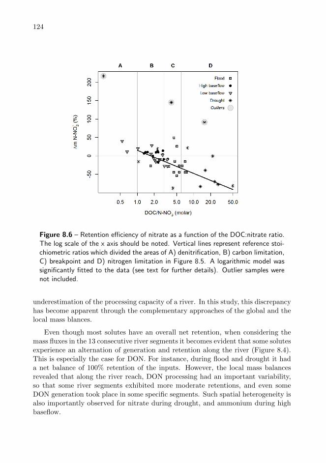
124
Figure 8.6 – Retention efficiency of nitrate as a function of the DOC:nitrate ratio.The log scale of the x axis should be noted. Vertical lines represent reference stoi-chiometric ratios which divided the areas of A) denitrification, B) carbon limitation,C) breakpoint and D) nitrogen limitation in Figure 8.5. A logarithmic model wassignificantly fitted to the data (see text for further details). Outlier samples werenot included.
underestimation of the processing capacity of a river. In this study, this discrepancyhas become apparent through the complementary approaches of the global and thelocal mass blances.
Even though most solutes have an overall net retention, when considering themass fluxes in the 13 consecutive river segments it becomes evident that some solutesexperience an alternation of generation and retention along the river (Figure 8.4).This is especially the case for DON. For instance, during flood and drought it hada net balance of 100% retention of the inputs. However, the local mass balancesrevealed that along the river reach, DON processing had an important variability,so that some river segments exhibited more moderate retentions, and even someDON generation took place in some specific segments. Such spatial heterogeneity isalso importantly observed for nitrate during drought, and ammonium during highbaseflow.

CHAPTER 8. DOM AND NITROGEN PROCESSING 125
Overall these results underline that in the occurrence of local heterogeneity, theglobal and the local scales may not be extrapolable between them. Similarly, in sedi-ment transport studies local variation was identified to produce large errors to wholereach mass balance calculations (Grams et al., 2013). Also, Moody et al. (2013)found evidences that catchments may be smaller DOC sinks than what is suggestedby whole-catchment mass balances if the DOC losses within the catchment streamsare taken into account. This evidences the key importance of spatial variability inchoosing the right scale for determining the boundaries in mass-balance studies inorder to make accurate determinations of the biogeochemical role of a river reachor chatchment.
Finally, we also found that hydrology intervenes, for every solute, in the extentof the spatial variability.
8.3.3 DOC mass balance
The importance of elucidating DOC mass balances in streams and rivers is widelyrecognised in the literature, but it is rarely empirically quantified (Moody et al.,2013). Among the few previous studies, DOC budgets are usually presented asannual budgets and have been performed using a whole catchment as a single blackbox. Thus annual DOC losses have been quantified from 12-18% in a 2-km riverreach (Dawson et al., 2001) to 40% in a peat catchment (Worrall et al., 2006) and31% accross the whole UK river network (Worrall et al., 2007). These figures areuseful to understand the carbon cycle at the big picture level, however, they lackresolution of spatiotemporal patterns in DOC processing. Eatherall et al. (2000)calculated net DOC in-stream losses during baseflow and flood conditions, andtheir results revealed a shift from a conservative (3% removal) to a sink behaviour(25% DOC removal). Their results emphasize the importance of the hydrologicalconditions in the net effect of the river passage on the DOC processing, even thoughthey find an opposite pattern compared to our results, that is, they find that highflows enhance the retention efficiency. However, they discuss the limitations of theirsampling strategy to capture all inputs of DOC along the catchment and highlightthe importance of detailed mass balance samplings in order to better determine thenet DOC processing.
On the other hand, to our knowledge our study is the first one to provide alongitudinal characterisation of DOC mass balance, under a range of hydrologicalconditions. We indeed found an important longitudinal variability in the biogeo-chemical processing of DOC in the river. Interestingly, all previous studies alwaysreport net losses for DOC, however in our study we detect net sources in the secondhalf of the river during flood conditions. The relevance of in-stream DOC sourcesis well documented in the literature (Bertilsson and Jones, 2003), as the periphy-
126
ton can be a relevant source of DOC. However it is surprising we detect DOC netsources during such high flow conditions, as it has been argued that in-stream pro-cesses would have their chance to occur relevantly at lower flows, when the residencetimes of DOC are higher and there are more opportunities for it to interact withthe environment (Battin et al., 2008).
Also, during the flood survey it is interesting to observe such gradual longitudinalvariation of the DOC processing efficiency, which shifts from retention in the up-stream segments to release or generation in the downstream segments. This gradualdownstream evolution suggests that changes in DOC processing during flood are notcontrolled by local drivers but rather by the different biogeochmical compartmentsflowing together downstream, i.e. they would be more related to planktonic-drivenchanges rather than benthonic-driven transformations. One reason supporting thisidea may be that during such high flows, the river bed sediments were importantlyresuspended and flowing downstream together with the water discharge and thesolutes within. However, it should be noted that efficiencies were low throughoutthe river reach (between -20% and 10%).
Contrastingly, during drought retention efficiencies were high in most river seg-ments, near 80% (Figure 8.3). Such high retention efficiencies, though, were reducedafter the outlets of the WWTPs of Sant Celoni and Hostalric. This effect has beenreported for inorganic solutes (Marti et al., 2004; Merseburger et al., 2011), howeverup to now it has not been explicitly evaluated for DOC. Even though sewage-treatedDOM has been described to be a labile (Fellman et al., 2009a, 2010) and photore-active fraction (Meng et al., 2013), such reduction in the removal efficiency maybe due to the high loads, which may saturate the in-stream capacity to processthe DOC inputs, similarly as for inorganic nutrients. The important lability maybe later reflected in the rapid recuperation of basal DOC removal in the next fewkilometers downstream.
8.3.4 Dissolved nitrogen mass balance
In contrast with DOC, DIN has received wider attention in river mass balancestudies. In Mediterranean rivers, the retention capacity of nitrate has been found tobe higher (23% and 52%, Aguilera et al. (2012) and Caille et al. (2012), respectively)than that found in other European watersheds, which have been estimated to bearound 10-20% (Grizzetti et al., 2005). Aguilera et al. (2012) argue that increasedretention efficiencies in Mediterranean watersheds may be due to the relativelylower flows with respect to the main European rivers. This agrees with the variableretention efficiency that we observed among hydrological conditions, especially forammonium which gradually varied from 15.2% retention during flood to 92.3%

CHAPTER 8. DOM AND NITROGEN PROCESSING 127
during drought. Nitrate remained relatively better conserved within the system, asfound in House and Warwick (1998).
In the spatial dimension, the effect of the WWTPs was less clear than wasobserved for DOC. In this case, an increase in the nitrogen concentration was trans-lated not only into a decrease in the retention efficiency, but even into a net releaseof nitrogen in that river segment. This occurs in the first, third and eleventh seg-ments. As mentioned, the third and the eleventh segments correspond with theinputs of the WWTPs of Sant Celoni and Hostalric, respectively. The first seg-ment, even though does not have any WWTP or industry, might have receivedsome point source anthropogenic input by the time the sampling was performed.Reduced retention efficiencies downstream of anthropogenic nitrogen inputs are inline with previous findings that nitrogen loading saturates the capacity of the bi-ological and physical uptake mechanisms (Martin et al., 2011; Marti et al., 2004;Merseburger et al., 2011).
8.3.5 Seasonal shift in the type of nitrogen retention
In all surveys nitrate was the most concentrated form of dissolved nitrogen. How-ever, the longitudinal profiles of nitrogen retentions revealed that it was usually theleast efficiently retained. Despite that, in absolute terms, during flood nitrate was,by far, the main form of retained nitrogen. In terms of retention efficiency, the mainform of nitrogen uptake changed from high (flood and high baseflow) to low flows(low baseflow and drought) along the 13 river segments. Specifically, there was ashift from DON to ammonium preferential uptake (Figure 8.2, third row).
During flood and high baseflow, DON was the most efficiently removed form ofnitrogen. Enhanced assimilatory DON uptake by heterotrophic bacteria, instead ofinorganic nitrogen, has been associated with either a limitation of carbon, whichcan inhibit denitrification (Johnson et al., 2012), or colimitation of carbon and in-organic nitrogen, which may favour assimilatory DON uptake (Lutz et al., 2011;Brookshire et al., 2005). Surprisingly, our results do not show any contrasting val-ues of ambient nitrate and DOC concentrations between the high and low baseflowsurveys. Carbon limitation could occur not only by changes in DOC concentration,but also by changes in its quality and lability. However our results do not showeither any changes in DOM lability specifically from high to low baseflow (Figure8.7) which could support such change in the preferred form of retained nitrogen.Otherwise, a simpler explanation would be that a change in the DON lability it-self occurred. In this case, a qualitative change was most likely to be blind tospectrophotometric methods. It has been reported that the main labile fraction ofDON are proteinaceous fractions contained in combined form (Maie et al., 2006; Yuet al., 2002) which may not be reflected in Excitation-Emission Matrices (EEMs)

128
Figure 8.7 – Average DOM quality of main stem sites in the mass balance surveys.High BF and Low BF refer to high baseflow and low baseflow, respectively
and therefore, in optical indices. Similarly, Inamdar et al. (2012) did not find anyassociation between DON and any EEM-derived metric.
On the other hand, in lower flows (low-baseflow and drought surveys), the high-est retention efficiencies were attributed to ammonium. This shift in the mainassimilated N form may be due to a series of modifications of the biophysical en-vironment following the flows decrease that favour ammonium retention. Namely,lower flowing velocities, shallow geomorphologies and high light availability favourthe proliferation of filamentous algae. The consequent high autotrophic activity maymodify the redox conditions in the sediments surface to more oxidising conditions,inhibiting denitrification (Arnon et al., 2013). Also, ammonium may be directlyassimilated by the algae, as most aquatic plant species prefer ammonia as nitrogennutrient (Kadlec and Knight, 1996). Finally, laminar flows may also maximize theabiotic retention of ammonium especially in adsorption to sediments due to its highadsorption capacity (Vogeler et al., 2011).
8.3.6 (Un)coupling between DOC and nitrate
General trends among major Earth ecosystems suggest that DOC can play a keyrole in regulating the accumulation of nitrate (e.g. DIN) in stream water (Taylorand Townsend, 2010; Goodale et al., 2005; Evans et al., 2006). It was consistentlyfound that nitrate accumulates at low DOC concentrations, whereas it is depletedat high DOC concentrations. A suite of microbial processes were identified as the

CHAPTER 8. DOM AND NITROGEN PROCESSING 129
underlying regulators of such stoichiometrically coupled behaviour between DOCand nitrate concentrations. However, these studies explicitly only used baseflowsamples in their models, and the role of hydrology was not specifically addressed.In this study, we contribute to fill this gap by comparing the behaviour betweenDOC and nitrate in different hydrological conditions, including extreme events likeflood and drought.
Our results show that DOC and nitrate concentrations from a Mediterraneanriver broadly have a similar behaviour as those from tropical, temperate, boreal andarctic regions (Taylor and Townsend, 2010). Visually, we identified a shift betweennitrate accumulation and depletion between the DOC:nitrate ratios 3 and 6, whichare in the lower limit of those identified across a range of aquatic biomes (Taylorand Townsend, 2010), which also correspond to the lowest C:N ratios observed inmicrobial tissues (Cleveland and Liptzin, 2007).
Within this general framework, in our system every specific hydrological sur-vey had a different DOC:nitrate stoichiometric relationship. During baseflow, therewas mostly an accumulation of nitrate. Samples exhibited concomitantly low DOCconcentrations (around 200 µmol/L), and DOC:nitrate ratios between 1 and 3-6.Between these ratios, carbon is considered to be the limitant for the microbial assim-ilatory activity (Taylor and Townsend, 2010). On the other hand, at DOC:nitrateratios higher than 6 – and therefore, in the area of nitrogen limitation – samplescorresponded exclusively to the drought survey. However, not all drought sampleshad such high ratios, but instead, appeared in all ranges of ratios: both in theregion of preferential denitrification (DOC:nitrate < 1), as well as in that of carbonlimitation (DOC:nitrate between 1 and 3-6) hence making it apparent that duringdrought there was a wide diversity of stoichiometric conditions.
At DOC:nitrate ratios lower than 1, it is considered that there are the optimalstoichiometric conditions for denitrification, and therefore nitrate should be min-imal. In our data set, most of the data are close or below the 1:1 line (Figurefig:DOCNNO3-retNNO3). Only two clear exceptions were observed, which mayconsist on sites that that received nitrate inputs recently upstream and therefore,stoichiometric ratios could still not adapt to general DOC:nitrate dynamics.
However, during flood samples did not fit the general framework of Taylor andTownsend (2010). In that survey, samples did not exhibit a negative nonlinearrelationship but, on the contrary, a positive linear trend was observed. One hy-pothesis would be that, under such extreme flash flood conditions, both nitrate andDOC would result from the rapid flushing of the terrestrial catchment, thereforeexhibiting such positive relationship (William and Grant, 1979; Martin and Harri-son, 2011; Hood et al., 2006). However, our results from the mass balance suggestthat, despite the rapid downstream water and solute transport, in-stream processingof carbon and nitrogen took place to an important extent. Therefore, our results

130
rather suggest a differentiated processing which modifies the relative carbon andnitrogen cycling, thereby altering the relationship between nitrate and DOC.
When relating the DOC:nitrate molar ratio with the nitrate mass flux, we ob-served a general negative linear trend and a continuum between the samples fromthe different surveys and, in this case, flood appeared integrated within the generaltrend. The general trend was consistent with our hypothesis and hence, with theframework of Taylor and Townsend (2010). That is, under a carbon stoichiometri-cal limitation, nitrate had a tendency to be neutrally transported or to have slightin-stream releases, whereas at higher DOC:nitrate ratios, nitrate had higher reten-tion efficiencies. Therefore, our mass-balance results support the hypothesis of astoichiometrical coupling between DOC and nitrate. In our river, the breakpointwas found to be at a DOC:nitrate ratio of 3, which corresponds to the lowest rangeof reported C:N ratios of microbial biomass (Cleveland and Liptzin, 2007). How-ever, drought did not follow the same trend as the flood and baseflow samples, asthey presented an important dispersion. Therefore, in that hydrological conditionthe relationship between the nitrate processing and the streamwater DOC:nitrateratio was not clear. It would be necessary to have more data on nitrate retentionefficiencies in order to draw conclusions with the same confidence as in the DOC vsnitrate concentrations relationship.
8.4 Conclusions
In this study, we described the longitudinal patterns of DOC and dissolved nitrogenconcentrations and mass balance along a 26 km river reach in a Mediterraneancatchment under a range of contrasting hydrological conditions. Our main findingshave been:
• Retention predominated for the dissolved nitrogen and organic carbon solutes.However, the efficiencies of the net retentions in the river were different ac-cording to the hydrological conditions: it was maximal during drought andminimal during flood.
• During flood, even though the processing efficiencies were the lowest amonghydrological conditions, in absolute terms it was the date in which the largestamount of nitrogen and DOC mass was retained and released, respectively.This emphasizes the importance of such extreme events, even if they last justfor some few hours or days.
• DON had a distinct behaviour with respect to DIN and DOC, as it exhibitedhigh net retentions in all hydrological conditions, as well as an importantspatial variability in its processing.

CHAPTER 8. DOM AND NITROGEN PROCESSING 131
• In space, the retained mass consistently increased downstream in all hydro-logical conditions. However, the main nitrogen solute removed in every surveydiffered. From flood to drought, they corresponded to nitrate, DON and am-monium.
• In terms of removal efficiencies, spatial patterns were not clear and had animportant longitudinal variability.
• In space, after the confluences with the WWTP inputs, there was a reducedretention efficiency both for DOC and dissolved nitrogen.
Regarding the coupling between DOC and nitrate:
• Our results showed that in the studied Mediterranean river, the stoichiomet-rical relationship between DOC and nitrate streamwater concentrations wasconsistent with that observed in the major Earth systems, especially duringbaseflow conditions.
• During flood, the general nonlinear negative trend was shifted to a linearpositive relationship.
• Results of the mass balance were consistent with the stoichiometric findings,and showed that nitrate processing changed into higher retention efficienciesat higher DOC:nitrate ratios. In this case, the drought period did not followthe general trend and showed a weak relationship between nitrate processingand DOC:nitrate stoichiometry.
• Finally, we emphasize the determinant role that hydrology plays in the defini-tion of longitudinal patterns of carbon and nitrogen biogeochemical process-ing, as well as in the definition of its coupling.

132

Chapter 9
Downstream processing ofDOM: changes in its reactivityand composition
9.1 Introduction
Understanding the fate of dissolved organic matter (DOM) in the environment iscurrently a major challenge, difficult to unveil due to the complex simultaneity ofdifferent biogeochemical processes in which it is involved, and to the uneven effectsthat they have on individual fractions of DOM. Often, DOM retention in space hasbeen modelled as a first-order decay function where it is assumed that the amountof retained DOM is a function of its own initial concentration (Raymond and Bauer,2000; Weyhenmeyer et al., 2012; Baldwin et al., 2014). However, DOM transforma-tions may follow more intricate longitudinal patterns due to the complexity of DOMenvironmental interactivity. The main processes responsible for the degradation ofDOM are the UV radiation and microbial activity, both of which have the capacityto completely oxidise DOM to CO2, as well as to alter its composition, as it hasbeen detectable in its fluorescence composition (Lee and Hur, 2014; Gao and Zepp,1998; Cory and Kaplan, 2012).
Bacteria have been widely recognised to be important DOM consumers, respon-sible for the re-introduction of organic carbon to the food webs (Azam et al., 1983),as well as to the outgassing of CO2 to the atmosphere (Battin et al., 2008; Tranviket al., 2009). Also, they can degrade and modify the quality of bulk DOM, andconvert it into more labile (Cammack et al., 2004; Guillemette and del Giorgio,2011) or recalcitrant (Ogawa et al., 2001) fractions. This traditional view of bacte-
133

134
Traditional view Recent evidences
Bacteria as consumers of DOM Dual role of bacteria as consumers and producersof DOM (Guillemette and del Giorgio, 2012)
Protein-like components as very la-bile fraction
Protein-like components can range from labile torecalcitrant. (Maie et al., 2007)
Humic-like fraction as a recalcitrantfraction
Humic-like fraction can be utilised and directlyoutgassed as CO2 (Fasching et al., 2014)
Microbially-derived components al-ways labile
Bacteria can produce recalcitrant humic-like com-ponents. (Jiao et al., 2010; Guillemette and delGiorgio, 2012; Fasching et al., 2014; Asmala et al.,2014)
Table 9.1 – Commonly accepted views regarding DOM sources and lability beingchallenged in recent studies.
ria eminently as consumers, though, is currently being revised due to the increasingevidences that bacteria have a dual role as consumers and as producers (Guillemetteand del Giorgio, 2012). On the one hand, they can produce protein-like compoundswhich have been traditionally considered to be highly labile and rapidly uptakenfrom the water (Rosenstock and Simon, 2001; Fellman et al., 2009b), even thoughit has also been found that a fraction of the protein-like components can includehumic molecules of low-molecular weight with a recalcitrant character (Maie et al.,2007; Cory and Kaplan, 2012). On the other hand, bacteria have also been foundto produce highly aromatic humic-like substances, which have been commonly at-tributed to be originated exclusively in terrestrial systems (Ogawa et al., 2001; Jiaoet al., 2010; Asmala et al., 2014) and to exhibit a recalcitrant character (Cory andKaplan, 2012). But recently, there are evidences that such humic-like substances,derived either from bacterial activity or the terrestrial drainage, can be utilised bybacteria under certain conditions and represent a potentially important pathway ofcarbon loss through outgassing as CO2 (Guillemette et al., 2013; Fasching et al.,2014). Overall these findings emphasize the difficulty to predict the fate of DOM infreshwater ecosystems (Table 9.1), as its lability is a highly relative concept whichdepends also on the structure and function of the microbial communities and theircapacity to degrade specific DOM compositions (Judd et al., 2006).
UV radiation has also been found to be an important process directly convertingDOM into CO2 (Miller and Zepp, 1995), or modifying its composition (Mostofaet al., 2007). Studies have demonstrated that sunlight breaks DOM molecules intoblue-shifted compounds (Lee and Hur, 2014) of lower-molecular weight (Osburnet al., 2001). The lability of DOM photoproducts have been found to range fromlabile (Moran and Zepp, 1997) to recalcitrant (Tranvik and Kokalj, 1998). Again,there is such an important specificity between the molecule being photodegraded,the nature of the photoproducts, and the microbial community present to utilise

CHAPTER 9. PROCESSING OF FLUORESCENT DOM 135
that material, that it is especially complex to predict what will be the fate of DOMin a natural system, subject to both photo- and bio-degradation.
Moreover, all the cited works assessing the relationship between DOM and bac-teria have tested their hypothesis using laboratory incubations thereby controllingthe environmental conditions. Such experiences are important because they eluci-date the potential interactivity between bacteria and DOM, however, it is difficult totranslate such potential observations to what effectively occurs in natural systems.
In this chapter we contribute to expand the understanding of DOM fate duringdownstream riverine transport by providing direct field evidence on the generationor retention of specific DOM fractions. For that, we use the mass balance approachof the previous chapters to evaluate the downstream reactivity of individual fluo-rescence components (as determined in chapter 4), and further, we test the role ofhydrological conditions in determining longitudinal reactivity patterns. The perfor-mance and suitability of SOM-derived fluorescence components has been previouslyassessed as shown in the Annex of this thesis.
Our aims are addressed according to the following specific objectives:
• To quantify the extent of in-stream processing of the DOM fluorescence com-ponents on the whole-reach scale: we first show the global effect of the passageof DOM along the whole river reach on each of the fluorescence components,considering it as a single black box. Next, we present the longitudinal pat-terns of generation/retention processes along the river reach, correspondingto the mass balances performed at each of the thirteen successive downstreamsegments.
• To assess the effect of hydrological conditions at shaping DOM processingboth at the reach (global) and at the segment (local) scale.
• To test the coupling between quantitative and qualitative DOM changes,both i) in terms of concentrations (for dissolved organic carbon (DOC) anddissolved organic nitrogen (DON)) and fluorescence intensities (fluorescencecomponents), and ii) in terms of generation or retention efficiencies.
• To assess to what extent the DOM processing in each river segment can bepredicted from its own initial characteristics in the beginning of each riversegment, in terms of i) initial concentrations and ii) initial character, as de-scribed by the optical indices Fluorescence Index (FI), Humification Index(HIX), Biological Index (BIX) and Specific Ultra-Violet Absorbance (SUVA).

136
9.2 Results
9.2.1 Fluorescence intensities of DOM components
The longitudinal profiles of the intensities of DOM components (Figure 9.1, firstrow) show that the four components followed similar trends downstream, but theirrelative intensities differed among surveys. During flood, the highest intensities werefound for component C3 (56.051 r.u.3nm−2), followed by C4 (32 839.8 r.u.3nm−2),that is, the humic-like fraction. Conversely, during high-, low-baseflow and drought,there was a predominance of the protein like fraction. C1 was the most intensecomponent (17 735.6, 12079.0 and 29660.2 ) followed by C2 (8220.2 , 10657.6 and18497.4 for high-, low-baseflow and drought, respectively).
The longitudinal profiles of the fluorescence intensities exhibited gradual down-stream evolutions during flood and the two baseflow surveys, with a slight increasingtrend. During baseflow, intensities (represented mainly by component C1) becamehigher in the last kilometres of the river reach (6.5 km in high baseflow and 11.5km in low baseflow). The effect of the waste water treatment plant (WWTP) ofSant Celoni (at 25 km from source) could be noted as a small peak, although verymodestly. During flood, such differentiation of the last km was not observed, butthere was rather a steady oscillation along the whole river length, with minimalvalues in the upstream-most sites.
During drought, such gradual downstream patterns were replaced by an impor-tant variability in the fluorescence intensities, consisting in two main peaks. Thefirst one, at 25 km from the river source, was located after the inputs from theWWTP of Sant Celoni, whereas the second one, at 40 km, appeared after the in-puts from the industrial area of Hostalric. In both cases, though, concentrationsrecuperated basal intensities in the following two sampling sites (within a 5 kmdownstream distance). The peak at 25 km was represented by all for componentsat similar proportions; however at 40 km the peak was mainly due to the increasein the fluorescence intensity of C1 and, to a lesser extent, of C2.
9.2.2 Global mass balance
If we consider the whole 26-km river reach as a big black box, we can comparethe total sum of the inputs (sum of the flow-weighted fluorescence intensities of thetributaries) with the outputs (flow-weighted fluorescence intensity flowing at thefinal main stem site, in Fogars de la Selva). The differences between the inputs andthe outputs for every fluorescence component and for every survey are presentedboth in absolute terms and as percentages with respect to the inputs, also hereafterreferred to as processing efficiencies (Table 9.2).

CHAPTER 9. PROCESSING OF FLUORESCENT DOM 137
Fig
ure
9.1
–F
luo
resc
ence
inte
nsi
tya
nd
ma
ssfl
uxe
sfo
rD
OM
flu
ore
scen
ceco
mp
on
ents
alo
ng
the
ma
inst
emo
fth
eT
ord
era
.F
irst
row
corr
esp
ond
sto
the
obse
rved
flu
ores
cen
cein
ten
siti
es;
seco
nd
and
thir
dro
ws
corr
esp
ond
toth
ed
iffer
ence
bet
wee
nth
ein
pu
tsan
dth
eou
tpu
tsat
ever
yri
ver
segm
ent
expr
esse
din
abso
lute
term
san
das
per
cen
tage
,re
spec
tive
ly.
Pos
itiv
eva
lues
ind
icat
ere
leas
eor
gen
erat
ion
,w
her
eas
neg
ativ
eva
lues
refe
rto
rete
nti
onor
assi
mila
tion
ofth
eco
mp
onen
ts.
Inal
lp
lots
,th
ed
iffer
ent
cate
gori
es(i
.e.
flu
ores
cen
ceco
mp
onen
ts)
are
stac
ked
.

138
Flood High baseflow Low baseflow DroughtSolute r.u.3nm−2 (×106)
C1 152.9 (5.4%) 46.2 (223%) 23.2 (107.8%) -4.4 (-37.3%)C2 172.2 (5.5%) 18.3 (90%) 11.1 (60.4%) -6.5 (-58.7%)C3 316.9 (3.7%) 10.6 (28.7%) 5.9 (24.5%) -5.6 (-50.8%)C4 289.7 (5.7%) 6.1 (25.5%) 0.4 (2.3%) -4.8 (-62.5%)
Table 9.2 – Global mass balance for the DOM fluorescence components.Values refer to the differences between the inputs and the outputs in the wholeriver reach, between brackets these differences are expressed as percentages withrespect to the inputs. Positive values indicate produced fluorescence intensity,whereas negative values indicate depleted fluorescence intensity during the riverinepassage.
During flood, the amount of processed fluorescence intensity in absolute termsrepresented the largest amounts of generated fluorescence intensity throughout thisstudy (in the order of 108r.u., Table 9.2). However, these generations, when com-pared to the inputs, correspond to very low generation efficiencies (3.7 to 5.7%)what suggests that in essence there is a conservative passage of the fluorescencecomponents through the riverine transit.
Under lower flows, processing efficiencies became prominent. During high- andlow-baseflow, the river represented a source of fluorescence intensity, especially forthe protein-like fractions: component C1 was tripled (+223.0 %) and duplicated(+107.8%) under high- and low-baseflow, respectively; and component C2 waspractically duplicated in both hydrological conditions (+90.0 % and +60.4%, re-spectively). Increases in the humic-like fraction were more moderate, exhibitingproductions between 20%-30%, with the exception of C4 during low-baseflow whichappeared conservative (2.3%).
During drought, the opposite trend occurred: All four components experiencedretentions during the riverine passage. The highest retention efficiency was observedfor the humic-like component C4 (-62.5 %), followed by the protein-like componentC2 (-58.7%). The component that underwent the least net retention rate was C1(-37.3%).
9.2.3 Longitudinal profiles of retention and release
The mass balances performed at 13 successive river segments refine the findings ofthe global mass balances (Figure 9.1, second and third rows) on the longitudinalperspective.

CHAPTER 9. PROCESSING OF FLUORESCENT DOM 139
During flood conditions, processing efficiencies for all four fluorescence compo-nents ranged between -60% to 39%, averaging -7.5% (Figure 9.2). These efficiencieswere much lower than those observed in the other surveys with lower flows. Inabsolute terms (Figure 9.1, second row) it can be seen that, despite the first half ofthe river reach exhibiting little fluorescence processing, the final half concentratesthe processing of large amounts of fluorecence intensity. Due to the low percentagesthat they represent with respect to the inputs (i.e. low processing efficiencies), itcannot be assured with enough confidence whether such differences in the inten-sities are due to ecological processes or analytical errors. However, in this secondhalf of the river, it is consistently observed that depletions occur for the protein-like fractions C1 and C2, whereas the humic-like components C4 and C5 undergonotable productions especially between the 7th and 10th segments (located at 31 to38.5 km from source). These results suggest that, despite an eminently conservativetransport, a weak DOM processing occurs in the middle sections of the river thatoperate differentially for the humic-like versus the protein-like components.
During baseflow, the river reach appeared clearly divided into two parts, bothin absolute and relative terms: a first part with little or nil processing, and asecond part undergoing important fluorescence intensity generations. During high-baseflow conditions, this final reactive part of the river reach spanned 3 segments(6.5 km long), whereas during low-baseflow it spanned a longer distance, including6 segments (11.5 km long). The main DOM fraction experiencing net generationsin these final river segments was the fluorescence component C1, followed by C2.By contrast, components C3 and C4 showed more moderate generation efficiencies.
Finally, during drought there were net depletions of all four fluorescence compo-nents in all segments (averaging -26.2 ± 82.8 % for C1, -46.7 ± 47.2 % for C2, -53.2± 24.2 % for C3 and -61.4 ± 21.7 % for C4, Figure 9.2). In some segments, thispattern was reduced (segment 3) or even inverted (segments 11 and 12) for compo-nents C1 and C2 (Figure 9.1). In segment 3, located at the outlet of the WWTPof Sant Celoni, processing efficiencies of all four components were reduced to verylow values, between -9.3% (C3) and 11.9% (C2), indicating a conservative trans-port of fluorescent DOM in these site. By contrast, in segments 11-12 (which followthe confluence with the Creek of Arbucies, including the outlet of the WWTP ofHostalric), retentions of protein-like fractions were inverted to generations of 167%(C1) and 45% (C2). Such important generations of protein-like intensity in thesesegments may balance the retentions experienced in the rest of segments, and mayexplain the fact that the net retentions in the whole river reach are lower for theprotein-like than the humic-like fraction. Indeed, if we compute the average re-tention among segments, excluding segments 3, 11 and 13, we obtain very similarretention efficiencies (-64.7 ± 21.0 % for C1, -69.9 ± 17.4 % for C2, -63.4 ± 13.7 %for C3 and -68.0 ± 12.0 % for C4). This emphasizes that, in the absence of direct

140
Figure 9.2 – Average retention efficiencies of the fluorescence components,for each of the four hydrological surveys. Every box represents de distribution of theefficiencies among the 13 river segments were local mass balances were performed.bfl stands for baseflow.
WWTP inputs, the four fluorescence components are indistinctly removed from theriver water.
9.2.4 Quantitative and qualitative coupling of DOM processing
Coupling between DOM concentrations and fluorescence components in-tensities
Linear models were computed between DOM concentration (as DOC and as DON)and the intensities of the fluorescence components along the middle reaches, in or-der to explore the relationships between quantitative and compositional aspects ofDOM. That is, linear correlations were computed between DOC or DON concen-tration, and the intensities of the fluorescence components.
When all the surveys were considered together, DOC concentrations had a strongpositive linear relationship with the fluorescence intensities of components C3 (R2 =0.942, p <0.001, df=51) and C4 (R2 =0.936, p <0.001, df=51; Figure 9.3A). Sam-ples sites exhibited a clear linear continuity where the samples from higher flowsappear at higher DOC concentrations and higher fluorescence intensities. However,this linear relationship was not observed for the protein-like components C1 andC2 (Figure 9.3B). For these components, the sites collected during drought, low-

CHAPTER 9. PROCESSING OF FLUORESCENT DOM 141
Figure 9.3 – Relationship between DOC concentration and the fluorescenceintensity of C4 (A) and C1 (B). The solid line in panel A describes the significantrelationship between DOC concentration and the fluorescence intensity of C4. Seetext for further details.
and high-baseflow exhibited a saturation curve, in which for fluorescence intensitiesbetween 0 and 104 r.u.3nm−2 DOC exhibited a coupled linear increase, whereas atfluorescence intensities higher than 104 r.u.3nm−2 DOC remained at concentrationsnear 2 mg L−1. On the other hand, the samples collected under flood did not ap-pear in this saturation curve, but as a cluster situated at higher DOC concentrations(9.29± 1.4mgL−1) and intermediate fluorescence intensities (15.6× 10³ ± 2.2× 10³
r.u.3nm−2). This indicates that, out of flood conditions, samples remained at lowDOC concentrations but variable degrees of protein-like fluorescence compounds,whereas during flood, there was an increase in DOC concentration which was notdirectly reflected as an increase in the protein-like fluorescence signal. Overall, therewas an uncoupling between DOC concentration and the protein-like fluorescence in-tensity, which was especially disrupted during flood conditions.
Contrastingly, when the qualitative-quantitative coupling was assessed withDON, no relationship was observed. The linear correlations between DON andthe fluorescence components always had R2 less than 0.132 and p higher than 0.07.The lack of any statistically significant correlation between DON concentration andthe fluorescence intensity of any of the fluorescence components highlighted the un-coupling between the fluorescence composition and the DON content in the samples.
Coupling between the processing of DOM and that of the fluorescencecomponents
Next the coupling between bulk DOM and the individual fluorescence componentswas assessed in terms of biogeochemical processing. This was addressed by com-puting linear models between the mass retentions/generations of DOC and DON,

142
Figure 9.4 – Relationship between the processing efficiency of DOC and C4.The solid line represents the significant linear correlation between both variables, seetext for further details. Every symbol represents a different hydrological condition,as defined in Figure 9.3.
versus the fluorescence intensity retentions/generations efficiencies of the fluores-cence components.
Similarly to what was observed in the previous section, the best correlationswere found between DOC and the humic-like components, although in this casewith a lower statistical strength. The processing of bulk DOC explained morethan 50% of the processing of the components C3 and C4 (for C3, R2 = 0.571,p = 9.6 × 10⁻¹¹, df=51; for C4, R2 = 0.740, p = 2.9 × 10⁻¹⁶, df=51; Figure 9.4).Conversely, no significant – or very weak statistical correlations were found for theprotein-like components (for C1, R2 = 0.089, p = 0.03, df=51; for C2, R2 = 0.277,p = 6.1× 10⁻⁵, df=51).
The graphical representation of the relationship between the processing of DOCand fluorescence components (Figure 9.4) reveals that the survey that mainly con-tributed to the linear relationship between both parameters is that of drought con-ditions. While the samples corresponding to the surveys of flood, high- and low-baseflow appear forming a cloud around the axis origin, those from drought appearlinearly distributed at the negative axis of both DOC and fluorescence componentsprocessing efficiencies, so that higher retentions of DOC implicated higher retentionsof the fluorescence components. This relationship could be perceived for all fluo-rescence components, but as mentioned it was maximised and statistically relevantfor C3 and C4.
The retained or produced mass of DON did not significantly correlate with thefluorescence intensity retention or release of any of the four components (R2 alwaysless than 0.084, and p always higher than 0.053).

CHAPTER 9. PROCESSING OF FLUORESCENT DOM 143
9.2.5 Can the input characteristics of DOM determine its down-stream biogeochemical processing?
Relationship between the initial intensities of DOM fluorescence compo-nents and their processing
Next it was assessed to what extent the degree of biogeochemical processing ofDOM was dependent on the initial concentrations at the beginning of every riversegment. Very similar patterns were found for DON, C3 and C4. In the case ofC4 (Figure 9.5) baseflow and flood samples did not show a clear trend but rathera cluster-like distribution centered near 0% of processing efficiency (5.76 ± 16.95%). However, they presented different fluorescence intensities at the beginning ofthe river segments: baseflow samples (both high- and low-baseflow) were centeredat 7801 ± 2038 r.u.3nm−2, whereas flood samples were centered at 32776 ± 4472r.u.3nm−2. However, during drought samples had some linear behaviour, so thathigher retention efficiencies were obtained for lower fluorescence intensities. Therewere some sites, though, that appeared as outliers to this linear trend. In the case ofthe fluorescence components C3 and C4, the outliers corresponded to the segment1 sampled during flood, and to the segments 3 and 11 sampled during drought. Inthe case of DOC, the outliers corresponded to the segments 3 and 12. Segment 1is located after the WWTP of Santa Maria de Palautordera, segment 3 after theWWTP of Sant Celoni, and segments 11 and 12 are located after the WWTP ofHostalric. These outlier sites appeared together with the samples collected duringhigh- and low- baseflow. Under such conditions, samples appeared clustered at lowintensities and low production/retention efficiencies.
Contrastingly, DON and components C1 and C2, did not show any relationshipbetween their processing percentage and their initial concentrations, at any of thesampled hydrological conditions.
Relationship between the optical indices and the processing of the fluo-rescence components
In order to answer this question, the correlations between the optical indices at thebeginning of every segment and the production/retention of fluorescence intensityfor the different fluorescence components were computed (Figure 9.6).
The most clear statistical relationship was found for the FI during drought (Fig-ure 9.6A), which could significantly explain the retentions of the four fluorescencecomponents. The strongest correlations were found for components C2 (R2 = 0.746,p = 6 × 10⁻⁴, df=10) and C3 (R2 = 0.731, p = 4 × 10⁻⁴, df=11). In the case ofC2, segments 3 and 11 were excluded as outliers, whereas for C3, segment 3 was ex-

144
Figure 9.5 – Relationship between the processing of C4 and its initial con-centrations. Every symbol represents a different hydrological condition, as definedin Figure 9.3.
cluded. For components C1 and C4, FI explained less than 70% of its variance (forC1, R2 = 0.673, p = 2× 10⁻³, df=10; for C5, R2 = 0.532, p = 7× 10⁻³, df=11). Inthe rest of surveys (that is, from low baseflow to flood), no statistical relationshipswere found, as the variability in the FI values were too small compared with thevariation in the retention/release of fluorescence intensity.
In the case of HIX, there was no significant statistical relationship with thebiogeochemical processing of any of the components. However, it could be ob-served that at higher values of HIX, the dispersion in the biogeochemical percent-ages gradually decreased, and became centered to zero, indicating a gradually lowerbiogeochemical processing of the fluorescence components towards higher HIX val-ues, represented by the flood samples (Figure 9.6B). This pattern could be observedfor all the four components.
Finally, SUVA and BIX did not have any statistically relevant ability to predictthe biogeochemical processing of fluorescence components.
9.3 Discussion
The main conclusion that can be drawn from the results of this chapter is that hy-drology plays a key role in determining both the global reactivity of the river reach,as well as the longitudinal distribution of such reactivity. This is especially impor-tant for systems like the Mediterranean ones, which are subject to high intra-annualhydrological variability; and provides further evidence that the biogeochemical func-tioning of these systems is tightly linked to hydrology.

CHAPTER 9. PROCESSING OF FLUORESCENT DOM 145
Figure 9.6 – Relationship between the processing of fluorescence componentC3 and the values of FI (A) and HIX (B) optical indices at the beginning ofthe river segments. In A, the solid line describes the relationship between bothvariables during drought conditions (see text for further details). Every symbolrepresents a different hydrological condition, as defined in Figure 9.3.
9.3.1 Hydrology and the biogeochemical processing of DOM fluo-rescence components
Baseflow
During baseflow conditions the river reach as a whole was found to be a net sourceof fluorescence components, especially of the protein-like component C1, followedby C2, but also of the humic-like components C3 and C4. This was an interestingresult given that for bulk DOM (that is, DOC and DON), the whole river reach wasnot found to be a net source in any of the hydrological conditions. This suggeststhat there are processes that operate modifying the composition of DOM withoutaltering its overall quantity. Therefore, this points to an uncoupling between thequantitative and the qualitative dynamics of DOM. The production of fluorescenceintensity of specific components parallel to bulk DOC decreases has already beenobserved (Asmala et al., 2014; Guillemette and del Giorgio, 2012) and has beenpointed to the capacity of microorganisms to convert uncoloured DOM forms intocoloured ones (Guillemette and del Giorgio, 2012). In the case of this study, mostof the produced intensity corresponded to protein-like components, what is in linewith common knowledge that protein-like substances are usually derived from au-tochthonous microbial activity (Henderson et al., 2009). However, to a lesser extentbut still remarkably, humic-like components were also generated. These findingsadd evidence to the recent revision of the traditional conception that humic-likesubstances are solely of terrestrial origin and that, on the contrary, microbial ac-tivity can be an important source of humic-like material (Ogawa et al., 2001; Jiaoet al., 2010).

146
The longitudinal profiles for the baseflow conditions showed that most of thisDOM production observed during high- and low-baseflow occurred in the final seg-ments of the river reach, which spanned the last 6.5 km during high baseflow, and11.5 km during low baseflow. That is, with lower flows the length of the final reac-tive part of the river became longer. This could be related to increased residencetimes in lower segments where the river morphology becomes shallower downstream,as it has been described that low residence times may favour the opportunities forDOM processing (Battin et al., 2008; Weyhenmeyer et al., 2012). Also, with thelengthening of the reactive part it could be observed that the generation percentageincreased gradually downstream, what suggested that downstream changes were notdirectly related to local features but rather to global environmental factors.
The fact that such generations were translated into higher fluorescence intensi-ties in stream water which remained downstream suggest that, at least to a certainextent, these in-stream generated components are persistent and therefore, recalci-trant to biological or photochemical degradation. This is in line with observationsthat microbially-produced protein-like or humic-like components can be persistentin the environment (Jiao et al., 2010; Maie et al., 2007).
The hydrological extremes: drought and flood
The opposite biogeochemical functioning was found during drought, when the riverreach as a whole behaved as a sink for the fluorescence components; in this case, con-sistently with what was found in quantitative terms for DOC and DON. However,retention efficiencies for the fluorescence components (ranging between 37.3% and62.5%) were much moderate than those observed for DOC and DON (which were of73.3% and 100%, respectively). This could be explained by two hypothesis: on theone hand, this could reflect that the fluorescence fraction of DOM is more refractorythan the non-fluorescence compounds. This would be in accordance with the gen-eral conception in the scientific literature that well-known biochemical compounds,most of which are not aromatic and hence, do not have fluorescence properties, arethe most labile and rapidly utilised fractions of DOM (Montuelle and Volat, 1993).On the other hand, another explanation would be that such reduced retention ef-ficiencies of the fluorescence components with respect to bulk DOC might be dueto parallel generations of fluorescence DOM which would counter-balance the netretentions. This second hypothesis would be sustained by our finding that, duringdrought, higher FI values are related to lower retention efficiencies (Figure 9.6), assuch relationship would indicate that lower net retentions are related to a higherprevalence of in-stream produced fluorescence DOM.
Along the longitudinal axis it was found that, similarly to what was observedfor DOC, after the confluences with the WWTP there was a decrease in the re-

CHAPTER 9. PROCESSING OF FLUORESCENT DOM 147
tention efficiency of the fluorescence components (segment 3, Sant Celoni), or evenan inversion into generation (segments 11-12, Hostalric). This further suggests asaturation in the system that surpasses the natural capacity of the river to uptakefluorescent DOM, as it has been similarly observed for inorganic nutrients (Martiet al., 2004; Martin and Harrison, 2011; Merseburger et al., 2011). In Sant Celonithe inputs from the WWTP were translated into an increase in the retention effi-ciencies of all four fluorescence components at similar proportions which, togetherwith a paractically null processing efficiency, suggests that in that site there wasonly a physical mixing of the inputs which caused the observed increase in the flu-orescence intensities. By contrast, in Hostalric there was mainly an increase in thefluorescence intensity of the protein-like components (mainly C1 but also C2), whichin this case were the result of in-stream generations, which could be triggered bythe inputs from the WWTP, which could have introduced either missing reactantsor a different microbial community capable of undergoing such important gener-ations of protein-like components (McClain et al., 2003). In both cases, though,such increases in the intensities of fluorescence components were rapidly depletedin the following downstream river segments, as evidenced by the net retentions andrapid recuperations of basal fluorescence intensities in the following segments. Over-all these results evidence a high lability of both the allochthonous/anthropogenicDOM inputs, and the in-stream generated fluorescence components.
Under flood conditions, the river reach as a whole behaved mainly as a pipe, asthe differences between the inputs from the tributaries, and the outputs at Fogarsde la Selva were practically identical (differences between 3.7% for C3 to 5.7% forC4, Table 9.2). In absolute terms, the river transported large amounts of fluorescentDOM downstream. To make these magnitudes more apparent, if we consider thatduring flood the river generated 289.7 r.u./s of C4, and that in drought the riverretained 4.8 r.u.3nm−2s−1, (Table 9.2) then it follows that in flood conditions theriver exported in 1s the same amount that it would be capable of retaining in 1minute during drought.
In the longitudinal perspective, it could be observed (similarly to what was foundfor baseflow conditions) a shift from a first part in which the river segments werevery conservative, and a second part where the segments were more reactive. Fluo-rescence generations were observed for the protein-like components, although theirmagnitudes represented little percentages with respect to the inputs and, therefore,such non-conservative transport could not be confidentially assumed. However,some retention was indeed likely to occur in the final reaches (7,8,9 and 12), for thehumic-like components C3 and C4.

148
9.3.2 Relevance of different hydrological conditions in the frame-work of the Mediterranean seasonality
Overall these results highlight the key role that the hydrological conditions play indetermining the biogeochemical processing of DOM. On the one hand, it determinesthe role of the whole river reach, as it shifts from behaving as a conservative pipeduring flood, to a source during baseflow, and to a sink during drought. On theother hand, it also determines how DOM processing is distributed in space.
Baseflow conditions are those that are most common throughout the year. Inthe last 10 years, La Tordera had water flows between those sampled during high-and low-baseflow surveys during 17.34 % of the days, although according to theoperational hydrological categories defined in the Materials and Methods (Chapter3, Figure 3.3) and used in chapters 5 and 6, baseflow conditions may represent theflows that occurred 45% of the days of the last 10 years. Under these circumstances,if we assume that the final quilometers of the river which were not included in themass balance behave like the second reactive part, then the river may mainly deliverfreshly produced protein-like components to the coast.
By contrast, floods are very short in time. The flows sampled in the floodsurvey have only been exceeded 0.18 % of the days during the last 10 years, andcould represent the flows of 5% of the days according to the categories definedin Figure 3.3. However such flash-flood episodes are very intense, and they canrepresent an important flux of DOM export in quantitative terms as it has beenwidely acknowledged in the literature (Dalzell et al., 2005; Wiegner et al., 2009;Wilson et al., 2013). However, in qualitative terms, it has been widely acceptedthat the rapid flash-floods transport DOM without much opportunities for its in-stream processing. Whereas here we did not obtain enough confidence to concludethe opposite, we did find trends that in the lower part of the river reach someprocessing of the fluorescence components took place. Future studies would benecessary to better assess to what extent any preprocessing of the DOM occursprior to be discharged to the coast under flash-flood circumstances.
Finally, drought conditions may span a variable length of time every year, typ-ically lasting up to 2 or 3 of months. The specific flows sampled in the droughtsurvey were equal or lower in 15.23 % of the days of the last 10 years, and couldrepresent up to 50% of the days (according to the categories defined in Figure3.3). During drought, DOM deliveries to the coast are minimal, as the river flowis rapidly reduced and completely depleted at the river mouth and an inland intru-sion of the river/sea water interface occurs (as was evidenced in chapter 5 with thehigh salinities at the last sampling sites during the drier periods). Therefore, undersuch circumstances the export of DOM from the land to the sea would be minimal,

CHAPTER 9. PROCESSING OF FLUORESCENT DOM 149
and, if still any flux of DOM would occur, it would deliver highly processed DOMmaterial.
Hence, these results highlight that hydrology determines a seasonality of thequantitative and qualitative delivery of DOM to the coastal system which maydetermine its temporal functioning.
9.3.3 Biogeochemical reactivity of DOM fluorescence components
Some of our findings support recent revisions of traditional conceptions about thesources and lability of fluorescence DOM components (Table 9.1). Specifically, wefound evidences for an important in-stream generation of fluorescence DOM whichcould be due to the recently described dual role of bacteria as consumers and asproducers (Guillemette and del Giorgio, 2012). The generation role of fluorescentDOM was especially apparent during baseflow conditions, when the fluorescencecomponents altogether increased by 75% (high baseflow) and 50% (low baseflow).Linked to that, we found evidences that the bacterially-derived components, beeither humic-like or protein-like, were likely to be recalcitrant, as net generationsremained at successive segments downstream. By contrast during drought the gen-eration of DOM could not be proved, as net depletions were observed. However,generations may be likely to occur, as their counter-balancing effect may explainthe relatively low retention efficiencies observed during drought.
On the other hand, we found a lack of relationship between the reactivity ofbulk DOC and DOM concentrations and their initial intensity at the beginningof every river segment. That is, the reactivity of bulk DOC and that of fluores-cence components could not be predicted from their initial characteristics. Suchrelationship would be expectable in case that their retention in space followed afirst-order decay function (Raymond and Bauer, 2000; Weyhenmeyer et al., 2012;Baldwin et al., 2014). The lack of such relationship in this study can be explainedby two assumptions: on the one hand, we found evidences of in-stream generationsof fluorescence DOM that would occur in parallel with DOM uptake, so that suchgenerations would blur the final net retentions detected. On the other hand, inevery segment there is a different time residence and, because of that, every pair ofretention efficiency and initial concentration may not be comparable.
Also, with the exception of FI during drought, optical indices did not explaineither the efficiencies of DOM processing. This emphasizes the decoupling betweenDOM composition and its lability in the environment, and further emphasizes thecomplexity and relativity of the lability concept.

150
9.4 Conclusions
The main conclusions that arouse in this chapter are the following:
• Hydrology is a key environmental factor that determines the transport andreactivity of DOM in the Mediterranean river under study.
• Whereas in terms of DOC and DON the river was found to behave as a pipeduring flood and high baseflow, and as a sink during drought, in terms offluorescence composition the river behaved as a pipe during flood, as a sourceduring baseflow, and as a sink during drought.
• Even though a reactive transport of fluorescence DOM during flood could notbe assessed with enough confidence, there were evidences of some protein-likedepletions and humic-like generations during the riverine passage.
• During baseflow conditions there were important generations of protein-likecomponents which triplicated (high-baseflow) and doubled (low-baseflow) theinputs. Humic-like components were also generated, although at lower effi-ciencies.
• In drought conditions, all four fluorescence components exhibited retentionsalong the river length, with the only exceptions of segments under the influenceof anthropogenic inputs, in which retentions were reduced or even inverted togenerations.
• In space, during flood and baseflow DOM processing occurred in the final seg-ments of the river reach. Contrastingly, during drought DOM reactivity tookplace homogeneously along the river reach, except in the anthropogenically-influenced segments.
• In our field observations, the degree of DOM processing could not be predictedfrom its initial characteristics (i.e. initial intensities and character in terms ofoptical indices).
• Some of our findings support recent revisions of traditional views, providingobservations which are in line with studies reporting a dual role of bacteriaas both consumers and producers of fluorescence DOM and a recalcitrantcharacter of in-stream produced components.

Chapter 10
General discussion
Dealing with dissolved organic matter (DOM) implies dealing with complex organicmolecules. This arises from the fact that DOM is composed of an amalgam of or-ganic molecules spanning a range of chemical structures – most of them unknownand highly humified (McDonald et al., 2004) – and also spanning a range of in-teractivity with the environment – as different groups of molecules will present avarying degree of susceptibility to be involved in different biogeochemical processes,whether microbial or photochemical degradation, sediment sorption or flocculation(Jaffe et al., 2008).
The main aim of this thesis was to better understand transport and reactivityof DOM during its downstream riverine passage, and to elucidate to what extentand in what manner hydrological conditions influence such downstream transportof DOM. Assessing the in-stream reactivity of DOM requires previous knowledgeabout its composition, as it is not enough to calculate the differences in overall DOMquantity (e.g. dissolved organic carbon (DOC)). Such difference would explain thenet amount of DOM which has been added or removed from the system. However,it would not explain underlying DOM transformations (Fisher et al., 2004). Micro-bial and photochemical degradation processes very often do not complete mineraliseDOM to CO2, but either break it into new compounds of lower molecular weight,or even aggregate and transform different molecules into larger and more complexcompounds (Bertilsson and Tranvik, 2000). These new molecules present a differ-ent ecological and biogeochemical role with respect to the original ones, as theywill subsequently have a different lability degree. Therefore, understanding DOMreactivity requires not only understanding quantitative changes, but also variationsin its composition.
151

152
10.1 Unveiling DOM composition: Self-Organising Mapsand correlation analysis
In order to study DOM, it is necessary to systematise and simplify the originallycomplex DOM composition into some few representative constituents which canthen be used as independent data variables. Such simplification is a key step, asit will determine our perception of DOM and, therefore, the knowledge that webuild about it. The challenge is to find a statistical methodology that performsthat simplification process in an objective way and that finds a number of DOMcomponents which are as representative as possible of the diversity of spectral shapesof a given data set.
Up to now, the main methodologies used for that purpose have been peak-pickingand parallel factor analysis (PARAFAC). Peak picking (Coble, 1996; Parlanti et al.,2000) reduces large Excitation-Emission Matrices (EEMs) into some few coordi-nates corresponding to peak maxima. Data reduction is important, but still thedefinition of a finite number of fluorescence components remains ambiguous and atthe subjectivity of the researcher. PARAFAC (Andersen and Bro, 2003; Stedmonand Bro, 2008) overcomes this limitation and resolves the overall signal of EEMsinto a number of fluorescence components that appear at fix coordinates among thesamples of an EEM data set. However, as this method is based on least squaressolutions, it is highly sensitive to the presence of outliers (Brereton, 2012). This isan important limitation, as it requires that experimental and sampling designs areplanned in order to suit PARAFAC requirements, namely, to span a gradual rangeof compositional changes (Stedmon and Bro, 2008). In this sense, we aimed at find-ing a tool which would give DOM researchers more freedom in their experimentaldesigns, and therefore, which would expand the number of research questions thatcan be addressed about DOM.
In chapter 4 we presented the use of self-organising maps (SOMs) (Kohonen,1998) to explore patterns in EEM data sets, as well as to resolve the compositionof DOM into some finite fluorescence components. SOM is an unsupervised self-learning algorithm that makes no preassumptions about the data structure, and hasa high flexibility to interpret and manage the results: it performs on the same time,a reduction of the dimensionality (distribution onto a two-dimensional grid) and aclustering (distribution among discrete units) of the original data, and offer manygraphical possibilities to explore and analyse results (Vesanto, 1999). It has alreadybeen used successfully in chemometrics (Brereton, 2012) for one (Mat-Desa et al.,2011) and two (Rhee et al., 2005; Bieroza et al., 2009) dimensional spectral datain order to find patterns among samples. Here, the novelty of our approach wasto couple SOM with a correlation analysis of its component planes (Barreto-Sanzand Perez-Uribe, 2007), so that a finite number of fluorescence components could

CHAPTER 10. GENERAL DISCUSSION 153
also be determined. According to our results, SOM had i) little outlier sensitivityand ii) enhanced resolution of component separation. The latter was possible dueto the re-weighting of the representativeness of different spectral shapes within thedata set, as the correlation analysis is performed on the codebooks of the SOManalysis, and not on the original samples. Even though in this thesis we did notpresent a systematic comparison between SOM and PARAFAC capabilities, wepreviously performed peak picking and PARAFAC analysis which produced weakerresults: with peak picking, there was a high dispersion in the peaks location thatcreated a lot of ambiguity to define different fluorescence components, whereas withPARAFAC, only two fluorescence components could be validated (Figure 10.1).Moreover, the two-component PARAFAC model produced systematic patterns inthe residuals matrices, indicating a weak fitting of the model (Stedmon and Bro,2008).
The SOM analysis presented in chapter 4 revealed the presence of four fluo-rescence components: two humic-like and two protein-like moieties, similar to thepreviously identified B, T, A and C components (here referred to as C1, C2, C3 andC4, respectively). These components were used thereafter in the rest of the thesis inorder to unveil their biogeochemical behaviour during their downstream transportin La Tordera, under three contrasting hydrological conditions: flood, baseflow anddrought.
10.2 Flood: Inert conduit of DOM from the land to thesea
In the mass balance study we had the opportunity to sample a very extreme floodevent. In Fogars de la Selva, the outlet of our mass balance design, there was adischarge of 156 m3s−1, a water flux that in the last 10 years has only been equalledor exceeded on three rainfall events (according the discharge data of the last 10years provided by Agencia Catalana de l’Aigua). However, this event may also berepresentative of stormflows of > 4m3s−1, as characterised in chapters 5 and 6. Suchflows occurred 5% of the days in the last 10 years, and represented the export of 40%of the total water, highlighting the relevance of the export capacity of stormflows,even though they are short in time. In such high flows, we observed an homogeneousDOM composition throughout the river length with a predominance of the humic-like components C3 and C4, together with a highly humified character as expressedby high Humification Index (HIX) values (chapters 5 and 6). Such homogeneitysuggested little processing during the DOM downstream transport under such highflows, assumption that was later demonstrated in the mass balance study.

154
Figure 10.1 – Different data mining methods applied to our EEM data set:peak picking analysis (A), PARAFAC (B) and SOM (C).

CHAPTER 10. GENERAL DISCUSSION 155
In chapters 8 and 9 we observed that the amount of DOM exported in Fogarsde la Selva was practically the same than the DOM that entered the river throughthe tributaries, both in terms of bulk DOM – for which the differences between theinputs and the outputs were -5.1 for DOC –, and of fluorescence components – forwhich the differences were -5.4 ± 0.3 % for C1, -5.5 ± 0.3 % for C2, -3.7 ± 0.2 %for C3 and -5.7 ± 0.3 % for C4. Such low percentages could still represent higheramounts of DOM retention than those reported in periods of lower flows, howeverthe uncertainties associated to those percentages do not allow to confidentially assessthe extent of such retention. The only exception to that eminent retentive characterwas dissolved organic nitrogen (DON), which exhibited a global depletion of 100%.
These results demonstrated that during flood, the river behaved eminently as apipe, inertly transporting DOM downstream. That is, during this flood event, everysecond the river was delivering at least 81 mg of highly humified, terrestrially-derivedDOC. If we assume that this behaviour can be made extensive for the stormflowsof > 4m3s−1 (as suggested in chapter 5), then the amount of exported DOM mayrepresent up to the 47% of the DOC export (computed over the last 10 years). Thelowland sites of the river were not included in the mass balance study, however if weconsider that the DOM composition remained homogeneous also in this final partof the river, we can assume that DOM was effectively discharged to the sea havingundergone hardly any processing.
10.3 Baseflow: Spatial variability of DOM transportand reactivity, and dual biogeochemical role of theriver
In chapter 5, the direct observation of the intensities of fluorescence DOM com-ponents revealed an important variability along the main stem, so that the riverhad three parts with clearly different DOM compositions. The headwaters had apredominance of humic-like materials, which reflected the drainage of the forestedland covers of the upper parts of the catchment. In Sant Celoni (the beginning ofthe middle part of the river) there was a change in the water chemistry, consistingin an increase in component C2, together with conservative anions (chlorides, sul-phates and electrical conductivity) as well as nutrients (nitrate, ammonium, solublereactive phosphor (SRP)). These increases indicated the predominance of inputs ofanthropogenic origin. Finally, in the lower part of the river, there was a predomi-nance of component C1 and increasing values of the Fluorescence Index (FI).
In fact, this approach provided evidence of the changing predominant sources ofDOM along the river: from terrestrial in the headwaters, to anthropogenic in themiddle reaches, and autochthonously-derived in the lower part of the river. This

156
emphasized that the variability of the concentrations and relative proportions offluorescence DOM components along the river were mainly driven by the predomi-nant sources. However, beyond a downstream switch in the main DOM sources, thedirect observation of the intensities of fluorescence components was not sufficientto demonstrate the extent at which DOM processing was taking place, and to whatextent any downstream compositional changes could be due simply to the physicalmixing of input waters providing a different water composition.
Some intuition in this sense was achieved by means of an end-member mixinganalysis (EMMA) approach. It was evidenced that the composition of some sitescould not be explained solely as the result of the mixing of upstream water in-puts, as they appeared outside of the endmember (i.e. tributaries) mixing domain.Therefore, the intensities of the fluroescence components had the be the result ofin-stream processing at least to some extent. This was most evident for the lowlandsites, and also expectable, as during the last 20 km the river flows along a mild ter-rain that hardly receives any tributaries. Hence, any observed increases in FI andC1 intensities should be due to in-stream processes. However, in the middle reachesthe degree of reactivity was less clear. Even though sites appeared mainly withinthe end-member mixing domain, on some dates during base flow and drought theyappeared highly disperse and outside it, suggesting that in-stream transformationscould be operating and shaping the main stem fluorescence intensities. Also, dueto the frequent confluences within the middle reaches, and to the different natureof their compositions, the relationship between transport and reactivity in this partof the river seemed less obvious.
The mass balance study (chapters 8 and 9) provided direct insight in this sense,and evidenced that an important in-stream processing of DOM took place. Mostremarkably, it was found that there was an uncoupling between the processingof bulk DOM and that of the individual fluorescence components. Bulk DOMexperienced moderate net retentions (differences of -9.8 during high baseflow and-21.2% during low baseflow for DOC between the total inputs and the outputs inFogars de la Selva). Contrastingly, fluorescence components experienced higherreactivity efficiencies, consisting on net generations. This was especially found forthe protein-like components which were tripled (C1) and doubled (C2) during theirriverine transport. Therefore, while the river was behaving as a moderate sink forbulk DOC, there were high generations of fluorescence components. This evidencedthe importance and relevance of intermediate transformations of DOM, rather thanits complete oxidation to CO2. Even though our sampling design does not allow toinfer what specific of biogeochemical processes were operating, our findings may addevidence to recent findings that bacteria can be important producers of fluorescenceDOM (Guillemette and del Giorgio, 2012).
CHAPTER 10. GENERAL DISCUSSION 157
In baseflow conditions, the global mass balances were representative of whatcould be observed locally, at the segment level. That is, locally we also observedgenerations of fluorescence DOM, mainly consisting on components C1 and to alesser extent, C2. However, such reactive processes only occurred in the final partof the middle reaches, which spanned 11.5 km during high baseflow (3.43 m3s−1)and 6.5 km during low baseflow (1.49 m3s−1), while in the previous segments therewas an eminent conservative transport of fluorescent DOM. If we assume that thereactivity that we observed in the final segments remains similar in the lower partof the river, then the DOM delivered to the coast will be rich in fresh and in-streamproduced protein-like components.
The two baseflow surveys performed during baseflow captured the discharges of1.49 and 3.43 m3s−1, therefore, the findings corresponding to these dates representthe state and functioning of the river at least 17.34 % of the days (according the dis-charge data of the last 10 years provided by Agencia Catalana de l’Aigua). Howeverthese findings may be extensive to the flows between 1 and 4 m3s−1, characterisedas baseflows in chapters 5 and 6. These conditions are mainly relevant due to theirduration over time and moderate flows, as they occurred 45% of the days during thelast 10 years, and exported 53% of the water, which in DOC terms, represents anexport capacity of up to one half of the total annual exported DOC (as computedover the last 10 years).
10.4 Drought: The river as a filter
During summer low flows, the spatial variability of DOM composition was similarto that observed during baseflow conditions. That is, a humic-like character in theheadwaters turned into a C2-dominated composition in the middle reaches and,finally, into a C1-dominated and high FI predomination in the lowland. However,such spatial differentiation and heterogeneity of DOM composition and characterwas maximised during drought, as shown in chapters 5 and 6.
Contrastingly with these heterogeneity in terms of DOM composition, in themass balance study it was found that in terms of biogeochemical functioning, therewas an eminent spatial homogeneity throughout the middle reaches. Globally, thispart of the river retained -73.7% of DOC, a similar percentage of the retentionthat the fluorescence components experienced, on average, in the different segmentsalong the middle reaches. Such longitudinal homogeneity was only disrupted at theoutlets of anthropogenic inputs. In Sant Celoni, the discharge of sewage water fromthe waste water treatment plant (WWTP) caused an interruption of the retentionsand, locally, DOC was conservatively transported. This was despite the fact thatin this site, important increases in DOM concentration and fluorescence intensities

158
were detected. The lack of retentions could be due to a decreased capacity of theriver to uptake DOM, similarly to what has been observed for inorganic nitrogen(Martin et al., 2011; Marti et al., 2004; Merseburger et al., 2011). By contrast, inHostalric, there was not just a depletion of the retention capacity but, conversely,there was a generation of fluorescence components and DOC. This suggests thatthere was not just a depletion of the retention capacity of the system, but rather,the anthropogenic inputs of DOM locally caused a differentiated biogeochemicalprocessing of DOM which resulted in a generation of protein-like moieties. Thiscould be due to some complementary effect between the DOM and/or bacterialinputs and those found in the river water which may have triggered the onset ofsuch protein-like DOM generation, as suggested in (McClain et al., 2003); eventhough it had little repercussion on the overall balance of DOM, as retention stillpredominated in the system as whole.
The behaviour of the river observed during drought conditions may be represen-tative of up to 50% of the days of the last 10 years, although due to the extreme lowflows these periods only account for 7% of the total exported water. Hence, duringsuch periods of minimal flows, the inputs of DOM to the coast are minimal, as theycontribute to approximately the 4% of the total DOC export (computed over thelast 10 years) and may deliver highly degraded organic materials.
10.5 The role of DOM in the regulation of inorganicnitrogen
Even though the main focus of this thesis is on DOM, its relationship with inor-ganic nitrogen has also been assessed, due to the coupled biogeochemical behaviourobserved between both kinds of substances (Lutz et al., 2011; Johnson et al., 2012).Globally it has been observed that nitrate accumulation in water bodies is regulatedby its stoichiometric relationship with DOM, as it regulates a suite of microbialprocesses that couple both substances (Taylor and Townsend, 2010). This resultsin an inverse and nonlinear relationship between nitrate and DOC concentrations(Goodale et al., 2005). However, such relationships have been assessed with base-flow conditions. In chapter 8 we assessed to what extent different and contrastinghydrological conditions fit into this stoichiometric framework, and to what extentchanges in the nitrogen mass fluxes could be related to changes in its stoichiometricrelationship with DOC.
Our results showed that despite most samples followed the nonlinear negativerelationship between the concentrations of DOC and nitrate previously describedin the literature (Goodale et al., 2005; Taylor and Townsend, 2010), flood condi-tions were an exception, and exhibited a positive linear relationship. We argued

CHAPTER 10. GENERAL DISCUSSION 159
that, most likely, the reason for this behaviour would be that the rapid downstreamtransport during such high flows do not allow for any biogeochemical coupling be-tween DOC and nitrate, and this may be supported by the low processing efficienciesfound for both in the global mass balances in flood conditions (-14.7% for nitrateand 5.1% for DOC).
On the other hand, the results of the mass balance study were consistent withthe stoichiometric findings, so that higher retention efficiencies of nitrate were foundat higher DOC:nitrate ratios. The samples from all the hydrological conditionscontributed to this relationship, even though during drought samples were moredispersed. However, overall these results highlight the role of DOM in coupling thecycles of carbon and nitrogen.
10.6 Implications and future research
Mediterranean rivers are highly dynamic systems over time due to the large intraan-ual variability of their flows regime, which have shaped its ecological structure andfunction (Gasith and Resh, 1999). In this thesis it has been evidenced that suchhydrological variability, unique of Mediterranean systems, has also a determinantrole in the biogeochemical functioning of rivers with respect to DOM. Whereas dur-ing extreme high flows downstream transport controls DOM export, during lowerflows in-stream processes dominate over transport and shape the quantity and com-position of the DOM that is finally exported from the river. Hence, the seasonalvariability of the Mediterranean river flows were found to have a determinant rolein shaping the quantity and quality of DOM which is finally exported to the sea:From large amounts of highly humified and little processed DOM during short andintensive storm events, to moderate amounts of protein-like and freshly producedDOM during baseflow, and small amounts of highly processed DOM during extremelow flows, that may extend up to half of the days of the year.
As rivers link the carbon cycle of the terrestrial and marine systems, it is ofutmost importance to better understand the consequences that such qualitatativechanges of DOM, derived from the riverine passage, have on the subsequent labilityof DOM in the sea. While there are evidences that marine bacterioplankton canreadily degrade riverine DOM (Bonilla-Findji et al., 2009) even at higher ratesthan riverine bacteria (Stepanauskas et al., 1999), the quality of exported DOMmay regulate the relative relevance of bacterial production and CO2 outgassing (Xuet al., 2014). Therefore, the observed seasonality in La Tordera of the quantityand quality of exported DOM to the coast may have complex repercussions on thecapacity of bacterial communities to degrade such temporally-changing DOM and,therefore, to further funnel DOM through the carbon cycle.

160
Unveiling the fate of riverine DOM in the sea involves facing a current chal-lenge of DOM research, which is to better understand the coupling between DOMcomposition and the structure and function of bacterial communities. DOM andbacteria have a close relationship as substrate - consumer, however such relation-ship, far from being straightforward, is intricate and recursive (Judd et al., 2006;Docherty et al., 2006) due to the plasticity of bacterial communities in their carbonmetabolism, allowing them to use DOM pools of different compositions (Rochelle-Newall et al., 2004). A better understanding on the adaptability of bacterial com-munities to changing characteristics of DOM may provide a better understandingon the lability of DOM, a concept that still remains relative to the specific bacterialcommunities and DOM pools sampled in every study.
Also, a better understanding of the coupling between DOM and bacteria mayprovide a further understanding of the underlying processes controlling the biogeo-chemical processing observed in this thesis. In this sense, this thesis contributedto expand the current knowledge about DOM transport and reactivity in lotic sys-tems by providing direct evidence of in-situ generation/retention of DOM fractionsalong a Mediterranean river. However, our field-based approach did not allow todiscern the specific biogeochemical processes (namely bacterial and photochemicaldegradation) that are directly controlling the observed retentions/productions, northe relative importance of each of them. Therefore, the findings of this work couldbe expanded by better understanding the controls that the bacterial communitiesexert on DOM composition and concentration.

Chapter 11
General conclusions
PART I
Chapter 4: Self-Organising Maps and correlation analysis for theanalysis of large and heterogeneous EEM data sets.
1. Self-organizing map (SOM) analysis coupled with a correlation analysis allowsan analysis both at the object and at the variable level. Hence, it serves notonly to explore the differences in fluorescence properties between samples, butalso helps to identify particular fluorescence components.
2. SOM analysis is robust to the presence of outliers. That is, samples with verydistinct features are discerned while having little effect on the ordination andclassification of the other samples. This distinct property makes it possible towork with heterogeneous data sets.
3. The correlation analysis performed on the SOM Excitation-Emission Matrix(EEM) prototypes has an enhanced capacity to detect fluorophores that arerepresented at only low levels in the original EEM data set.
4. SOM analysis coupled with a correlation analysis of the component planesexpands the toolbox of the fluorescence dissolved organic matter (DOM) re-searchers by enabling the analysis of complex and heterogeneous EEM datasets. This may open new possibilities for advancing our understanding ofDOM character and biogeochemical behaviour.
PART II
Chapter 5: Preliminary assessment of spatiotemporal patterns ofDOM quality and quantity in La Tordera
161

162
5. Along the main stem, the river exhibited three reaches with a consistent dif-ferentiated DOM character: the headwaters, the region near the town of SantCeloni, and the low part of the river flowing between the bend of Fogars de laSelva and the river mouth.
6. In the headwaters, DOM has an eminent humic-like character coming from thedrainage of the surrounding terrestrial catchment. During flood conditions,this character is transferred downstream.
7. Near Sant Celoni, there is a shift in the DOM quality, expressed as a pre-dominance in the protein-like component C2. A concomitant increase in thechlorides and nutrients content of the water suggests that this shift in theDOM quality is caused by the direct outlets of a waste water treatment plant(WWTP) and possibly other industries in the beginning of the river reach.
8. In the lower part of the river, high water residence times and light availabil-ity favour the conditions for in-stream DOM production and transformation,which results in an increased Fluorescence Index (FI) and predominance ofthe protein-like EEM component C1.
9. Whereas flood conditions induce an homogenisation of the DOM characterover the longitudinal dimension, baseflow and drought favour spatial differen-tiation resulting from the influence of the local characteristics of the river atevery reach.
10. The hydrological antecedents of a drought period determine the magnitude ofthe spatial differentiation of DOM character. A longer previous dry periodcontributed to an amplification of the longitudinal differentiation.
11. This suggests a seasonal role of the river with respect to DOM, shifting be-tween transporter and transformer. Such alternation in the transport andprocessing of DOM can have further implications for the understanding of thecarbon cycling at higher scales, and may contribute to the ongoing debate onthe role of inland waters on the global carbon cycle.
Chapter 6: Multivariate exploration of DOM quality and reac-tivity in the main stem of La Tordera
12. The homogenisation of DOM properties observed along the river length dur-ing flood conditions has been effectively found to be due to a conservativetransport.
13. The longitudinal patchiness in DOM properties that appears at lower flows donot only reflect the successive mixing with tributaries providing DOM withvarying properties, but are also due to the occurrence of in-stream processing.

CHAPTER 11. GENERAL CONCLUSIONS 163
14. The lowland sites, located between Fogars de la Selva and the river mouth,exhibited a downstream DOM gradient mainly driven by in-stream processing.
15. The headwater sites exhibited consistently a humified humic-like characterirrespective of the hydrological conditions, with conservative transport beingthe main driver of DOM downstream evolution.
16. The sites from the middle reaches were found to respond to a more intri-cate relationship between physical mixing and processing, due to the highfrequency of tributary inputs providing a variety of water types, from low tohighly polluted.
PART III
Chapter 7:Water balance in the middle reaches of La Tordera
During flood, high and low baseflow:
17. Most of the water inputs to the main stem of La Tordera come from thenatural drainage of the terrestrial catchment, mainly through the creeks ofArbucies and Santa Coloma.
18. The main stem discharge is the result of the sum of the previous water inputsreceived upstream. This indicates a minor interaction between the river andthe underlying alluvial and groundwater aquifers.
19. Under these circumstances, the cumulative approach is useful to predict lon-gitudinal changes in water and conservative solutes along the main stem.
Conversely, during summer drought:
20. Most of the water inputs to the main stem come from anthropogenic sources(either WWTPs or industries). The contribution of these inputs may beessential to maintain the flows in certain sections of the river.
21. The river exhibits important interactions with the underlying aquifers, linkedto the geo-tectonic structure of the physical environment. Because of that,there is an important spatial heterogeneity of the hydrological behaviour ofthe river, alternating between a gaining and a loosing character.
22. Despite the occurrence of a net infiltration of water over the whole length ofthe river reach, there are some specific spots that have an effluent character,located consistently with previous findings in the literature.

164
23. Under these circumstances, a reach-by-reach approach has been found to benecessary to predict longitudinal changes in water and conservative solutesalong the main stem, in order to take into account local water gains andlosses.
Chapter 8: Carbon and nitrogen mass balance: Linking DOCand nitrate
24. Retention predominated for the dissolved nitrogen and organic carbon solutes.However, the efficiencies of the net retentions in the river were different ac-cording to the hydrological conditions: it was maximal during drought andminimal during flood.
25. During flood, even though the processing efficiencies were the lowest amonghydrological conditions, in absolute terms it was the date in which the largestamount of nitrogen and dissolved organic carbon (DOC) mass was retainedand released, respectively. This emphasizes the importance of such extremeevents, even if they last just for some few hours or days (as floods).
26. dissolved organic nitrogen (DON) had a distinct behaviour with respect todissolved inorganic nitrogen (DIN) and DOC, as it exhibited high net reten-tions in all hydrological conditions, as well as an important spatial variabilityin its processing.
27. In space, the retained mass consistently increased downstream in all hydro-logical conditions. However, the main nitrogen solute removed in every surveydiffered. From flood to drought, they corresponded to nitrate, DON and am-monium.
28. In terms of removal efficiencies, spatial patterns were not clear and had animportant longitudinal variability.
29. In space, after the confluences with the WWTP inputs, there was a reducedretention efficiency both for DOC and dissolved nitrogen.
Regarding the coupling between DOC and nitrate:
30. In La Tordera, the stoichiometrical relationship between DOC and nitratestreamwater concentrations was consistent with that observed in the majorEarth aquatic systems, especially during baseflow conditions.
31. During flood, the general nonlinear negative trend was shifted to a linearpositive relationship.

CHAPTER 11. GENERAL CONCLUSIONS 165
32. Results of the mass balance were consistent with the stoichiometric findings,and showed that nitrate processing changed into higher retention efficienciesat higher DOC:nitrate ratios. In this case, the drought period did not followthe general trend and showed a weak relationship between nitrate processingand DOC:nitrate stoichiometry.
33. Results emphasize the determinant role that hydrology plays in the definitionof longitudinal patterns of carbon and nitrogen biogeochemical processing, aswell as in the definition of its coupling.
Chapter 9: Downstream processing of DOM: changes in its reac-tivity and composition
34. Hydrology is a key environmental factor that determines the transport andreactivity of DOM in the studied Mediterranean river.
35. Whereas in terms of DOC and DON the river was found to behave as a pipeduring flood and high baseflow, and as a sink during drought, in terms offluorescence composition the river behaved as a pipe during flood, as a sourceduring baseflow, and as a sink during drought.
36. Even though a reactive transport of fluorescence DOM during flood could notbe assessed with enough confidence, there were evidences of some protein-likedepletions and humic-like generations during the riverine passage.
37. During baseflow conditions there were important generations of protein-likecomponents which triplicated (high-baseflow) and doubled (low-baseflow) theinputs. Humic-like components were also generated, although at lower effi-ciencies.
38. In drought conditions, all four fluorescence components exhibited retentionsalong the river length, with the only exceptions of segments under the influenceof anthropogenic inputs, in which retentions were reduced or even inverted togenerations.
39. In space, during flood and baseflow DOM processing occurred in the final seg-ments of the river reach. Contrastingly, during drought DOM reactivity tookplace homogeneously along the river reach, except in the anthropogenically-influenced segments.
40. In our field observations, the degree of DOM processing could not be predictedfrom its initial characteristics (i.e. initial intensities and character in terms ofoptical indices).

166
41. Some of our findings support recent revisions of traditional views, providingobservations which are in line with studies reporting a dual role of bacteriaas both consumers and producers of fluorescence DOM and a recalcitrantcharacter of in-stream produced components.

Appendix
167


Evaluation of the capacity ofDOM optical variables toquantify mixing processes
Introduction
One of the main challenges for unveiling the role of dissolved organic matter (DOM)in rivers, is to understand its sources and fate. In this context, spectroscopic DOMmeasurements have found their success, because of their ability to detect DOMmoieties from different sources in a DOM mixture, and to track them after mixing.This fingerprinting capacity has been used and addressed in a number of studies,aiming at tracking downstream the impact of sewage (Baker, 2001; Borisover et al.,2011; Carstea et al., 2009), farm wastes (Bilal et al., 2010; Ruggiero et al., 2006;Naden et al., 2010), the contribution of different flowpaths to the river dischargeduring stormflow events (Fellman et al., 2009b; Hood et al., 2006; Nguyen et al.,2010) or to discern an authochthonous versus allochthonous production of DOM(Battin, 1998; McKnight et al., 2001). For that, a large variety of discriminationindices have been used, like the Fluorescence Index (FI) (McKnight et al., 2001;Carstea et al., 2009), the Humification Index (HIX) (Nguyen et al., 2010), the Spe-cific Ultra-Violet Absorbance (SUVA) (Hood et al., 2006) and the intensity or ratiobetween parallel factor analysis (PARAFAC) components (Fellman et al., 2009b;Borisover et al., 2011), as well as between fluorescence components determined byfluorescence regional integration (FRI) (Bilal et al., 2010).
Despite the numerous evidences that fluorescence measurements can serve asa good tool to track DOM from different sources, most studies have remained ata qualitatiave stage. Only few examples can be cited that tested the capabilitiesof fluorescence metrics to quantify mixing processes at subtle levels, and, most ofthem highlighted that their use should be critically examined (Yang and Hur, 2014).In order for a variable to have good discrimination capabilities, it should follow a
169

170
property balance principle; that is, it should exhibit a linear response at intermedi-ate mixtures of two or more DOM sources. Some studies, like in Hur et al. (2006),Korak et al. (2014) and Yang and Hur (2014) tested the discrimination capacity ofa several optical metrics using an end member validation approach was used. Thatis, well-defined end-member samples were used to create intermediate artificial mix-tures at known proportions in order to check the capacity of different indices topredict their values for intermediate mixtures. Hur et al. (2006) evaluated a totalof 18 metrics corresponding to HPLC-SEC chromatograms, fluorescence and ab-sorbance spectra. Yang and Hur (2014) tested the property balance of PARAFACcomponents, absorption coefficients, spectral slopes, peak ratios, HIX and FI, andKorak et al. (2014) tested the performance of fluorescence components determinedby visual peak-picking, as well as the FI index. Their work shows that not all thevariables are equally valid for predicting mixtures by mass-balance. Property bal-ance was found to be well preserved for fluorescence components, either determinedby PARAFAC (Yang and Hur, 2014) or visual peak picking (Korak et al., 2014).However, the discrimination capacity of indices based on spectral ratios showed avariety of behaviours. Hur et al. (2006) observed a good property balance for SUVAand a fulvic- to protein-like ratio, whereas FI and HIX have not been found to ex-hibit a linear behaviour with respect to end-member mixing ratios (Hur et al., 2006;Yang and Hur, 2014).
As self-organizing map (SOM) analysis is a novel approach to determine Excitation-Emission Matrix (EEM) components, we consider it necessary to evaluate the be-haviour of such components in mixing processes. Also, given that there are fewprevious studies testing the discrimination capacity of optical indices, and thatthere are some disparities in their results, we also test the performance of SUVA,FI and HIX. For the SOM components, we used two methods to quantify them:maximal fluorescence intensity, and regional integration. The former method sim-ply takes the maximal fluorescence intensity of every component region, and followsthe traditional peak-picking approach; while the latter integrates the area under thesurface of every component region using a Riemann summation as described in Chenet al. (2003). This will allow to compare the performance of the two quantificationmethods in mass-balance calculations.
Objectives
The specific objectives of this appendix are:
• To test the source discrimination capacity of the fluorescence componentsdetermined using Self-Organising Maps and correlation analysis (chapter 4).

ANNEX. QUANTIFICATION OF DOM MIXING PROCESSES 171
• To test the best quantification of SOM components in order to optimise theirdiscrimination capactiy: maximal intensity of regional integration.
• To test the property balance performance of other optical variables, namelySUVA, FI HIX and Biological Index (BIX), in order to provide more experi-ences to the scientific literature.
The results of this analysis will provide the basis to decide which variables aresuitable to be used in the DOM mass-balance study, chapters 9.
Procedures
In order to verify the linear relationship of an optical variable during DOM mixingfrom different sources, we performed two artificial mixture banks. The first oneused as end-members a sample from the effluent of the waste water treatment plant(WWTP) of Sant Celoni, and a pristine river water, corresponding to the creekof Fuirosos. The second mixture bank used as end-members the same WWTPeffluent, with a slightly impacted river water, corresponding the creek of Pertegas.The WWTP of Sant Celoni and the creek of Pertegas are located upstream of siteA3 (Figure 3.5), the creek of Fuirosos corresponds to site A6 (Figure 3.5).
End-member samples were collected in the field as described in section 3.3.Every pair of end-members were mixed at proportions of 100:0, 99:1, 90:10, 70:30,50:50, 30:70, 10:90, 1:99, 0:100; and after that, all mixtures were analysed for EEMfluorescence, absorbance spectra and dissolved organic carbon (DOC) concentrationas described in section 3.3. Next, expected values at intermediate mixtures werecalculated according to standard mass-balance calculations:
Cpredicted =C1 × V1 + C2 × V2
V1 + V2(11.1)
where C corresponds to a spectral variable or index, C1 and C2 the values of thespectral variable of each end-member and V1 and V2 the proportional volumes ofeach end-member in the mixture. Finally, the expected values were compared withthe measured ones by linear regression.

172
Results and discussion
EEM components
The EEMs of the end-members and some of the intermediate mixtures are shownin Table 11.1. The EEM of Fuirosos exhibited two peaks centered at λex = 240 and350 nm for λem=450. These correspond to peaks A and C (Coble, 1996), largelyreported for streams draining forested catchments (Hudson et al., 2007; Vazquezet al., 2011). On the other hand, the end-member from Pertegas had an additionalpeak at λex, λem = 290, 420, closer to the coordinates previously identified as peakM (Coble, 1996). This third peak lied near peak C with slightly higher intensity,therefore confering a shoulder-like shape to peak C. Finally, the end-member fromthe WWTP had a clearly distinct EEM shape. It showed 5 peaks, 3 of them centeredat λem = 425 nm and exciting at λex = 320, 270 and 240; whereas the other twowere centered at λem = 350 nm, exciting at λex = 285 and 240 nm. The firstthree appeared at the lower emission range for humic-like substances, whereas thelatter two appeared to the coordinates attributed to tryptophan-like material. Thehumic-like and the protein-like moieties appeared with similar intensity, what hasbeen identified as a typical feature of sewage DOM (Baker, 2001; Henderson et al.,2009). Throughout the intermediate mixtures between the WWTP and Fuirosos orPertegas, it can be seen that the characteristic shape of the WWTP was alreadyapparent at low proportions of this end-member.
In Table 11.2 there is a summary of the linear regression models between themeasured and the predicted values of the EEM components. In the first two groupsof rows appear the results for the EEM components determined by SOM. It isnoticeable that both types of quantification (i.e. maximal intensity or regional inte-gration) have very high goodness-of-fit values (r2 > 0.9900) and mean % differenceslower than 10%. This indicates the good ability for both quantifications to predictthe composition of end-member EEM mixtures. Moreover, the slope remains near1, indicating that there is no consistent pattern toward over- or underestimatingthe predicted values with respect to the actual ones.
Despite the high performance of the SOM components under both types ofquantification, a closer look to the mean % differences between the predicted andobserved values, indicates that in the quantification using maximal intensity values,the mean % differences are slightly higher than in the quantification using regionalintegration. Such trend is statistically significant for the Pertegas - WWTP mixtures(t-test, p < 0.05). Therefore, regional integration would be preferable to picking themaximal intensity of a SOM region, as it seems to be able to provide more accuratepredictions.

ANNEX. QUANTIFICATION OF DOM MIXING PROCESSES 173
Fuir
oso
s:
WW
TP
100
:0
70
:30
50
:50
30
:70
0:
100
Pert
egas
:W
WT
P100
:0
70
:30
50
:50
30
:70
0:
100
Ta
ble
11
.1–
EE
Ms
ofth
een
d-m
emb
ers
and
som
eof
the
inte
rmed
iate
mix
ture
s.

174
Fuirosos - WWTP Pertegas - WWTP
variable r2 slopemean %difference∗
r2 slopemean %difference∗
C1.vol 0.9970 0.974 7.80 0.9983 1.009 5.98C2.vol 0.9966 0.963 7.97 0.9981 1.01 6.63C3.vol 0.9986 0.985 2.36 0.9966 1.025 5.49C4.vol 0.9987 0.998 1.9 0.9974 1.009 4.13
C1.int 0.9945 0.961 9.36 0.9973 0.999 5.92C2.int 0.9965 0.959 6.83 0.9945 1.002 6.46C3.int 0.9980 1.004 2.31 0.9699 1.044 9.9C4.int 0.9943 1.016 5.83 0.9976 1.017 7.58
FI 0.9745 1.000 1.29 0.8236 0.921 3.89HIX 0.4848 0.533 40.99 0.4891 0.561 46.54BIX 0.5161 0.532 6.48 0.5592 0.637 7.98
SUVA 0.0355 1.066 6.09 0.1855 0.663 2.90
Table 11.2 – Summary of the linear model parameters for the different variablesevaluated. ∗ Percentage differences between the predicted and the measured values.
Among fluorescence components, the mean % difference between actual and pre-dicted values remains similar for the four components in the intermediate mixturesof Pertegas : WWTP. However, in the intermediate mixtures of Fuirosos : WWTP,the protein-like components (C1.vol and C2.vol, C1.int and C2.int) have a higher% difference than their corresponding humic-like components. This is evident inthe two types of EEM components determination (maximal intensities and regionalintegration), but slightly more accentuated with the components determined bymaximal intensity. This indicates that while the humic-like fraction behaves con-sistently in a linearly additive way, the protein-like substances are more prone tonon-linearity additions in mixtures. In order to better understand this phenomena,it is worth doing an attentive inspection of the expected versus the actual valuesof the intermediate mixtures (Tables 11.3, 11.4 and 11.5). In there it can be seenthat those mixtures containing the highest proportions of river water with respectto WWTP water (99:1 to 70:30), also have the highest mean % differences betweenthe actual and the predicted vaues. This is especially notorious for protein-likecomponents, which can have mean % differences up to 20 - 50 %. In contrast, di-lutions from 50:50 to 1:99 (predominance of WWTP water) have very low mean %differences (< 5%) indicating very accurate predictions in this range.
This asymetry over the range of mixing proportions could be attributable to thelarge differences between the end-members. However, this asymetric response wasalso evident in many of the variables evaluated by Hur et al. (2006), even thoughthey were working with two end-members of more similar nature (humic acids and

ANNEX. QUANTIFICATION OF DOM MIXING PROCESSES 175
fulvic acids, standards from the International Humic Substances Society (IHSS) andSigma-Aldrich respectively). According to that, this asymetry is more likely to beindependent of the original composition of the end-members, and more subject tothe behaviour of fluorescence to mixing processes.
Differentiated prediction capacity among SOM components
The high overall capacity of fluorescence components to predict the composition ofintermediate mixtures, implies the assumption that the EEM shape results fromthe linear sum of independently fluorescing components. This is indeed one of themain premises assumed in current DOM research methods, like PARAFAC, peakpicking and the fingerprinting approaches mentioned in the introduction.
However, in this study a further in-depth analysis of the mixing process showedthat the prediction accuracy was unequal at varying proportions of the end-members.These observations, consistent with findings in Hur et al. (2006), may unveil theoccurrence of intramolecular electronic interactions, which may ultimately affectthe fluorescence of the bulk DOM mixture (Del Vecchio and Blough, 2004; Boyleet al., 2009).
Whether the fluorescence of bulk DOM results from an non-interactive or inter-active sum of individual components is currently a matter of debate (Murphy et al.,2014). The role of electronic interactions such as intramolecular energy transfer,spectral shifting and charge transfer have been evidenced in laboratory analysesperformed at very controlled chemical conditions (Del Vecchio and Blough, 2004;Boyle et al., 2009; Ma et al., 2010). On the other hand, the non-interacting additiveapproach has predominated in field-based research and has triggered substantial ad-vances over the last decade (Fellman et al., 2010). In our results, the non-interactiveaddition approach appears to have the main role, as it explains more than the 99%of the data variability, Table. 11.2). However, the influence of non-interactive phe-nomena may explain the subtle poorer predictions observed in certain end-memberproportions.
Spectral indices
In contrast with EEM components, the spectral indices exhibited a poor capacityto predict the quality of DOM in intermediate mixtures. Out of the four studiedindicies, FI is the one which has the best linear adjust, with a high r2, a slope of1 and a very low mean mean % difference (1.29, Table 11.2). The r2, though, isslightly lower than those observed for EEM components (0.9745). This indicatesthat, even though it shows a good linear additive behaviour, its behaviour in massbalances should be interpreted in terms of trends, rather than for fine quantification

176
purposes. The authors of the FI index themselves (McKnight et al., 2001) discouragethe use of this index to quantify the relative proportions of precursor end-membersof a given sample. They state that the quantitative use of FI is influenced by theDOC concentration and the variation in fluorescence intensity per mg C of thedifferent fulvic acids. Korak et al. (2014) has found that FI behaves non-linearlywith end-member mixing ratios, and they attribute that to the fact that both theemission at with peak C has its maximal intensity, as well as its curvature, varysimultaneously. Because of that, the fluorescence intensities at the coordinates ofthe numerator and the denominator used to calculate the FI change at differentrates and this causes the non-linearity behaviour along a mixing gradient. Becauseof this reason, Yang and Hur (2014) found that all the metrics based on a spectralratio had a poor balance property, and this may also explain what we observe forthe rest of optical indices.
SUVA, like FI exhibited good prediction capability, observed from the low mean% difference (6.09). However, the very low r2 reveals a lack of linear additivity overthe end-member mixtures. Interestingly, this contradicts the findings of Hur et al.(2006), who found SUVA to be the best parameters performing linear additions.In view of the above-mentioned reasoning, this disparity could be due to the factthat in the set of mixtures used in Hur et al. (2006) the rate of change of DOCconcentration and the absorbance coefficent at 254 nm may be more moderate thanin our case.
HIX has no linear behaviour (r2 =0.4848 and 0.4891) and has extremely lowprediction capacity (mean % difference of 40.99 - 46.54). Therefore, in our study thisvariable should be discarded to be used in mass-balance calculations. Similarly, BIXalso showed a poor linear additive character, with an r2 of 0.5161 and 0.5592 andslopes near to 1, although the average percentage differences between the expectedand the observed values where not as high as for HIX. This poor source discriminantbehaviour is in line with the findings of Yang and Hur (2014) and may also beexplained by the fact that they are calculated as a ratio between two spectral regionsof different rates of change.
Conclusions
The specific findings of this annex include:
• EEM components were found to have a more robust linear additive behaviourirrespective of their method of determination (maximal intensity or regionalintegration). By contrast, the spectral indices, showed a weak (FI) or noability (HIX and SUVA) to predict values in mixtures.

ANNEX. QUANTIFICATION OF DOM MIXING PROCESSES 177
• Among spectral indices, FI was the only one that exhibited linear behaviour.However, its weak linear fit discourages its use in mass-balance calculations.
• The SOM components determined by regional integration obtained the highestaccuracies in the linear models (r2 > 0.99, mean % difference < 5%). Thisfurther underlines the potential of the use of the SOM analysis resolve EEMsinto meaningful components.
• By comparing between the four components, the protein-like fraction wasfound to be more prone to non-linear additivity, despite a good overall linearfit.

178
Fuirosos : WWTP Pertegas : WWTPMeasured Predicted Diff.(%) Measured Predicted Diff.(%)
C1.vol 100 : 0 2667 2667 n.a.(∗) 2100 2100 n.a.99 : 1 4709 3137 33.3 3171 2557 19.3
90 : 10 8250 7372 10.6 5747 6667 1670 : 30 14529 16782 15.5 17760 15800 1150 : 50 24997 26193 4.7 25668 24933 2.830 : 70 34964 35603 1.8 34206 34066 0.410 : 90 44216 45013 1.8 44277 43198 2.41 : 99 48025 49248 2.5 48242 47308 1.9
0 : 100 49718 49718 n.a. 47765 47765 n.a.
C2.vol 100 : 0 3496 3496 n.a. 2270 2270 n.a.99 : 1 6100 3973 34.8 3703 2738 26
90 : 10 9512 8267 13 6228 6953 11.670 : 30 15720 17808 13.2 18524 16319 11.950 : 50 26440 27350 3.4 26667 25686 3.630 : 70 36107 36892 2.1 35503 35052 1.210 : 90 45132 46434 2.8 45865 44418 3.11 : 99 49494 50728 2.4 49824 48633 2.3
0 : 100 51205 51205 n.a. 49102 49102 n.a.
C3.vol 100 : 0 12534 12534 n.a. 9408 9408 n.a.99 : 1 13561 13077 3.5 8851 9999 12.9
90 : 10 18765 17966 4.2 12547 15322 22.170 : 30 26958 28829 6.9 25562 27150 6.250 : 50 38396 39693 3.3 41984 38979 7.130 : 70 50416 50556 0.2 50820 50807 010 : 90 60658 61420 1.2 63079 62635 0.71 : 99 65057 66309 1.9 67679 67958 0.4
0 : 100 66852 66852 n.a. 68550 68550 n.a.
C4.vol 100 : 0 7425 7425 n.a. 4474 4474 n.a.99 : 1 7951 7766 2.3 4633 4843 4.5
90 : 10 10998 10833 1.5 6714 8160 21.570 : 30 16344 17649 7.9 17251 15532 9.950 : 50 23529 24466 3.9 22833 22904 0.330 : 70 31007 31282 0.8 30202 30277 0.210 : 90 37937 38098 0.4 37974 37649 0.81 : 99 41027 41166 0.3 40960 40966 0
0 : 100 41506 41506 n.a. 41335 41335 n.a.
Table 11.3 – Measured and predicted values calculated using mass balance (Eq.11.1), for the SOM components determined by regional integration. (∗) n.a. standsfor not applicable.

ANNEX. QUANTIFICATION OF DOM MIXING PROCESSES 179
Fuirosos : WWTP Pertegas : WWTPMeasured Predicted Diff.(%) Measured Predicted Diff.(%)
C1.int 100 : 0 0.127 0.127 n.a.(∗) 0.104 0.104 n.a.99 : 1 0.292 0.147 49.7 0.152 0.123 19.3
90 : 10 0.370 0.322 12.8 0.264 0.295 11.770 : 30 0.634 0.713 12.4 0.763 0.677 11.250 : 50 1.050 1.103 5 1.154 1.059 8.230 : 70 1.469 1.493 1.6 1.458 1.441 1.110 : 90 1.868 1.883 0.8 1.850 1.823 1.41 : 99 2.019 2.059 1.9 2.003 1.995 0.4
0 : 100 2.078 2.078 n.a. 2.014 2.014 n.a.
C2.int 100 : 0 0.222 0.222 n.a. 0.150 0.150 n.a.99 : 1 0.309 0.244 21.1 0.224 0.171 23.6
90 : 10 0.485 0.437 9.9 0.335 0.358 6.970 : 30 0.770 0.866 12.4 0.859 0.775 9.750 : 50 1.223 1.295 5.8 1.380 1.192 13.530 : 70 1.644 1.724 4.8 1.601 1.609 0.410 : 90 2.077 2.153 3.6 2.073 2.026 2.21 : 99 2.257 2.346 3.9 2.256 2.213 1.8
0 : 100 2.367 2.367 n.a. 2.234 2.234 n.a.
C3.int 100 : 0 0.584 0.584 n.a. 0.505 0.505 n.a.99 : 1 0.590 0.607 2.8 0.385 0.529 37.4
90 : 10 0.809 0.811 0.2 0.595 0.741 24.670 : 30 1.151 1.263 9.7 1.189 1.213 250 : 50 1.642 1.716 4.5 2.169 1.685 22.330 : 70 2.099 2.169 3.3 2.191 2.157 1.510 : 90 2.617 2.622 0.1 2.651 2.629 0.81 : 99 2.818 2.825 0.2 2.827 2.841 0.5
0 : 100 2.848 2.848 n.a. 2.865 2.865 n.a.
C4.int 100 : 0 0.553 0.553 n.a. 0.367 0.367 n.a.99 : 1 0.580 0.587 1.3 0.351 0.403 15
90 : 10 0.800 0.899 12.3 0.508 0.729 43.470 : 30 1.276 1.590 24.6 1.512 1.454 3.850 : 50 2.059 2.282 10.8 2.089 2.178 4.230 : 70 2.888 2.973 2.9 2.859 2.902 1.510 : 90 3.642 3.665 0.6 3.625 3.627 01 : 99 3.973 3.976 0 3.937 3.952 0.3
0 : 100 4.010 4.010 n.a. 3.989 3.989 n.a.
Table 11.4 – Measured and predicted values calculated using mass balance (Eq.11.1), for the maximal intensity of the SOM components (∗) n.a. stands for notapplicable.

180
Fuirosos : WWTP Pertegas : WWTPMeasured Predicted Diff.(%) Measured Predicted Diff.(%)
FI 100 : 0 1.56 1.56 n.a.∗ 1.48 1.48 n.a.99 : 1 1.55 1.57 0.9 1.49 1.49 0.2
90 : 10 1.63 1.6 1.6 1.64 1.53 6.670 : 30 1.72 1.68 2.4 1.83 1.62 11.650 : 50 1.82 1.76 3.1 1.88 1.71 8.930 : 70 1.89 1.84 2.6 1.91 1.8 5.610 : 90 1.94 1.92 0.7 1.92 1.89 1.81 : 99 1.95 1.96 0.3 1.93 1.93 0.3
0 : 100 1.96 1.96 n.a. 1.93 1.93 n.a.
HIX 100 : 0 17.64 17.64 n.a. 18.19 18.19 n.a.99 : 1 8.7 17.53 101.4 10.57 18.08 71
90 : 10 9.67 16.52 70.8 8.79 17.05 93.970 : 30 8.66 14.28 64.7 7.7 14.77 91.650 : 50 6.95 12.03 73 6.91 12.49 80.730 : 70 6.72 9.79 45.7 6.69 10.21 52.710 : 90 6.66 7.55 13.2 6.43 7.93 23.21 : 99 6.55 6.54 0.1 6.53 6.91 5.8
0 : 100 6.42 6.42 n.a. 6.79 6.79 n.a.
SUVA 100 : 0 3.84 3.84 n.a. 3.74 3.74 n.a.99 : 1 4.09 3.84 6 3.83 3.74 2.4
90 : 10 3.9 3.83 1.9 4.08 3.76 7.870 : 30 4.34 3.81 12.2 3.8 3.81 0.350 : 50 4.48 3.79 15.3 4.11 3.86 5.930 : 70 4.2 3.77 10.2 4.22 3.91 7.310 : 90 3.95 3.75 5.1 4.01 3.96 1.21 : 99 3.9 3.74 4.1 3.93 3.98 1.2
0 : 100 3.73 3.73 n.a. 3.98 3.98 n.a.
BIX 100 to 0 0.65 0.65 n.a. 0.64 0.64 n.a.99 to 1 0.80 0.66 17.8 0.75 0.64 14.6
90 to 10 0.80 0.67 15.2 0.79 0.66 16.770 to 30 0.79 0.71 9.6 0.82 0.70 15.250 to 50 0.84 0.75 10.2 0.83 0.73 11.230 to 70 0.83 0.79 4.4 0.84 0.77 7.810 to 90 0.84 0.83 0.5 0.86 0.81 51 to 99 0.85 0.85 0.6 0.84 0.83 1.3
0 to 100 0.85 0.85 n.a. 0.83 0.83 n.a.
Table 11.5 – Measured and predicted values calculated using mass balance (Eq.11.1), for spectral indices. ∗ n.a. stands for not applicable.

Bibliography
181


Bibliography
ACA. Consulta de dades - Xarxes de control, 2013. URL aca-web.gencat.cat/aca/.
Rosana Aguilera, Rafael Marce, and Sergi Sabater. Linking in-stream nutrientflux to land use and inter-annual hydrological variability at the watershed scale.The Science of the total environment, 440:72–81, 2012. ISSN 1879-1026. doi:10.1016/j.scitotenv.2012.08.030.
Hassan a Al-Reasi, Chris M Wood, and D Scott Smith. Physicochemical and spec-troscopic properties of natural organic matter (NOM) from various sources andimplications for ameliorative effects on metal toxicity to aquatic biota. Aquatictoxicology (Amsterdam, Netherlands), 103(3-4):179–90, June 2011. ISSN 1879-1514. doi: 10.1016/j.aquatox.2011.02.015. URL http://www.ncbi.nlm.nih.gov/
pubmed/21470554.
RB Alexander, RA Smith, and GE Schwarz. Effect of stream channel size on thedelivery of nitrogen to the Gulf of Mexico. Nature, 403(February):758–761, 2000.URL http://www.nature.com/nature/journal/v403/n6771/abs/403758a0.html.
Rainer MW Amon and Ronald Benner. Bacterial utilization of different size classesof dissolved organic matter. Limnology and . . . , 41(1):41–51, 1996. URL http:
//www.riversystems.washington.edu/lc/RIVERS/77\_amon\_rmw\_41-41-51.pdf.
C M Andersen and R Bro. Practical aspects of PARAFAC modeling of fluorescenceexcitation-emission data. Journal of Chemometrics, 17(4):200–215, 2003. ISSN0886-9383. doi: 10.1002/cem.790.
Shai Arnon, Keren Yanuka, and Ali Nejidat. Impact of overlying water velocityon ammonium uptake by benthic biofilms. Hydrological Processes, 27(4):570–578,February 2013. ISSN 08856087. doi: 10.1002/hyp.9239. URL http://doi.wiley.
com/10.1002/hyp.9239.
E. Asmala, R. Autio, H. Kaartokallio, C. a. Stedmon, and D. N. Thomas. Pro-cessing of humic-rich riverine dissolved organic matter by estuarine bacteria: ef-fects of predegradation and inorganic nutrients. Aquatic Sciences, 76(3):451–463, February 2014. ISSN 1015-1621. doi: 10.1007/s00027-014-0346-7. URLhttp://link.springer.com/10.1007/s00027-014-0346-7.
Kari Austnes, Christopher D Evans, Caroline Eliot-Laize, Pamela S Naden, andGareth H Old. Effects of storm events on mobilisation and in-stream processing ofdissolved organic matter (DOM) in a Welsh peatland catchment. Biogeochemistry,99(1-3):157–173, 2010. ISSN 0168-2563. doi: 10.1007/s10533-009-9399-4.
183

F Azam, T Fenchel, J G Field, J S Gray, L A Meyerreil, and F Thingstad. TheEcological Role of Water-Column Microbes in the Sea. Marine Ecology-ProgressSeries, 10(3):257–263, 1983. ISSN 0171-8630. doi: 10.3354/meps010257.
A Baker. Fluorescence excitation-emission matrix characterization of some sewage-impacted rivers. Environmental science & technology, 35(5):948–953, 2001. ISSN0013-936X. doi: 10.1021/es000177t.
A Baker. Fluorescence properties of some farm wastes: implications for waterquality monitoring. Water research, 36(1):189–195, January 2002. ISSN 0043-1354. doi: 10.1016/S0043-1354(01)00210-X.
A Baker and R G M Spencer. Characterization of dissolved organic matter fromsource to sea using fluorescence and absorbance spectroscopy. Science of the TotalEnvironment, 333(1-3):217–232, October 2004. ISSN 0048-9697. doi: 10.1016/j.scitotenv.2004.04.013.
Darren S. Baldwin, Kerry L. Whitworth, and Claire L. Hockley. Uptake of dissolvedorganic carbon by biofilms provides insights into the potential impact of loss oflarge woody debris on the functioning of lowland rivers. Freshwater Biology, 59(4):692–702, April 2014. ISSN 00465070. doi: 10.1111/fwb.12296. URL http:
//doi.wiley.com/10.1111/fwb.12296.
Miguel A Barreto-Sanz and Andres Perez-Uribe. Improving the correlation huntingin a large quantity of SOM - Component planes classification of agro-ecologicalvariables related with productivity in the sugar cane culture. LECTURE NOTESIN COMPUTER SCIENCE, 4669:379–388, 2007. ISSN 0302-9743; 978-3-540-74693-5.
Frauke K Barthold, Christoph Tyralla, Katrin Schneider, Kellie B Vache, Hans-Georg Frede, and Lutz Breuer. How many tracers do we need for end membermixing analysis (EMMA)? A sensitivity analysis. Water Resources Research, 47:W08519–W08519, August 2011. ISSN 0043-1397. doi: 10.1029/2011WR010604.
T J Battin. Dissolved organic matter and its optical properties in a blackwatertributary of the upper Orinoco river, Venezuela. Organic Geochemistry, 28(9-10):561–569, 1998. ISSN 0146-6380. doi: 10.1016/S0146-6380(98)00028-X.
Tom J Battin, Louis A Kaplan, Stuart Findlay, Charles S Hopkinson, EugeniaMarti, Aaron I Packman, J Denis Newbold, and Francesc Sabater. Biophysicalcontrols on organic carbon fluxes in fluvial networks. Nature Geoscience, 1(2):95–100, 2008. ISSN 1752-0894. doi: 10.1038/ngeo101.
Tom J Battin, Sebastiaan Luyssaert, Louis A Kaplan, Anthony K Aufdenkampe,Andreas Richter, and Lars J Tranvik. The boundless carbon cycle. Nature Geo-science, 2(9):598–600, 2009. ISSN 1752-0894. doi: 10.1038/ngeo618.
184

L Benda, K Andras, D Miller, and P Bigelow. Confluence effects in rivers: In-teractions of basin scale, network geometry, and disturbance regimes. WaterResources Research, 40(5):W05402–W05402, May 2004. ISSN 0043-1397. doi:10.1029/2003WR002583.
R Benner. Chemical composition and reactivity. In DA Hansell and CA Carlson,editors, Biogeochemistry of Marine Dissolved Organic Matter, chapter 3, pages59–90. Academic Press, Elsevier Science, New York, 2002. ISBN 978-0-12-323841-2.
S Bertilsson and L J Tranvik. Photochemical transformation of dissolved organicmatter in lakes. Limnology and Oceanography, 45(4):753–762, 2000. ISSN 0024-3590.
Stefan Bertilsson and Jeremy B. Jones. Supply of Dissolved Organic Matter toAquatic Ecosystems: Autochthonous Sources. In Stuart Findlay and Robert LSinsabaugh, editors, Aquatic Ecosystems: Interactivity of Dissolved Organic Mat-ter. Elsevier, 2003.
M Bieroza, A Baker, and J Bridgeman. New data mining and calibration approachesto the assessment of water treatment efficiency. Advances in Engineering Soft-ware, 44(1):126–135, February 2012. ISSN 0965-9978. doi: 10.1016/j.advengsoft.2011.05.031.
Magdalena Bieroza, Andy Baker, and John Bridgeman. Exploratory analysis ofexcitation-emission matrix fluorescence spectra with self-organizing maps as abasis for determination of organic matter removal efficiency at water treatmentworks. Journal of Geophysical Research-Biogeosciences, 114:G00F07–G00F07,December 2009. ISSN 0148-0227. doi: 10.1029/2009JG000940.
Magdalena Bieroza, Andy Baker, and John Bridgeman. Classification and cal-ibration of organic matter fluorescence data with multiway analysis methodsand artificial neural networks: an operational tool for improved drinking wa-ter treatment. Environmetrics, 22(3):256–270, May 2011. ISSN 1180-4009. doi:10.1002/env.1045.
Muhammad Bilal, Anne Jaffrezic, Yves Dudal, Cedric Le Guillou, Safya Menasseri,and Christian Walter. Discrimination of Farm Waste Contamination by Fluores-cence Spectroscopy Coupled with Multivariate Analysis during a BiodegradationStudy. Journal of Agricultural and Food Chemistry, 58(5):3093–3100, March 2010.ISSN 0021-8561. doi: 10.1021/jf903872r.
Martı Boada. Unitats de paisatge diferenciades: els cursos de la Tordera. In MartıBoada, Sılvia Mayo, and Roser Maneja, editors, Els sistemes socioecologics de la
185

conca de la Tordera, page 541. Institucio Catalana d’Historia Natural, Barcelona,first edit edition, 2008. ISBN 978-84-7283-983-0.
J R Boehme and P G Coble. Characterization of colored dissolved organic matterusing high-energy laser fragmentation. Environmental science & technology, 34(15):3283–3290, August 2000. ISSN 0013-936X. doi: 10.1021/es9911263.
Oriol Bolos. La vegetacio del Montseny. Servei de Parcs Naturals. Diputacio deBarcelona., Barcelona, 1983.
O Bonilla-Findji, E Rochelle-Newall, Mg Weinbauer, Md Pizay, Me Kerros, andJp Gattuso. Effect of seawater–freshwater cross-transplantations on viral dy-namics and bacterial diversity and production. Aquatic Microbial Ecology, 54(January):1–11, January 2009. ISSN 0948-3055. doi: 10.3354/ame01256. URLhttp://www.int-res.com/abstracts/ame/v54/n1/p1-11/.
Mikhail Borisover, Yael Laor, Ibrahim Saadi, Marcos Lado, and NadezhdaBukhanovsky. Tracing Organic Footprints from Industrial Effluent Dischargein Recalcitrant Riverine Chromophoric Dissolved Organic Matter. Water Airand Soil Pollution, 222(1-4):255–269, November 2011. ISSN 0049-6979. doi:10.1007/s11270-011-0821-x.
a. F. Bouwman, M. F. P. Bierkens, J. Griffioen, M. M. Hefting, J. J. Middelburg,H. Middelkoop, and C. P. Slomp. Nutrient dynamics, transfer and retention alongthe aquatic continuum from land to ocean: towards integration of ecological andbiogeochemical models. Biogeosciences, 10(1):1–22, January 2013. ISSN 1726-4189. doi: 10.5194/bg-10-1-2013. URL http://www.biogeosciences.net/10/1/
2013/.
Erin S Boyle, Nicolas Guerriero, Anthony Thiallet, Rossana Del Vecchio, and Neil VBlough. Optical Properties of Humic Substances and CDOM: Relation to Struc-ture. Environmental science & technology, 43(7):2262–2268, April 2009. ISSN0013-936X. doi: 10.1021/es803264g.
Richard G Brereton. Self organising maps for visualising and modelling. Chem-istry Central journal, 6 Suppl 2(Suppl 2):S1, January 2012. ISSN 1752-153X.doi: 10.1186/1752-153X-6-S2-S1. URL http://www.pubmedcentral.nih.gov/
articlerender.fcgi?artid=3395104\&tool=pmcentrez\&rendertype=abstract.
Rasmus Bro. PARAFAC. Tutorial and applications. Chemometrics and IntelligentLaboratory Systems, 38(2):149–171, 1997. URL http://www.sciencedirect.com/
science/article/pii/S0169743997000324.
Rasmus Bro and Maider Vidal. EEMizer: Automated modeling of fluorescenceEEM data. Chemometrics and Intelligent Laboratory Systems, 106(1):86–92,
186
March 2011. ISSN 01697439. doi: 10.1016/j.chemolab.2010.06.005. URLhttp://linkinghub.elsevier.com/retrieve/pii/S0169743910001152.
Marjorie L Brooks, Diane M McKnight, and William H Clements. Photochemicalcontrol of copper complexation by dissolved organic matter in Rocky Mountainstreams, Colorado. Limnology and Oceanography, 52(2):766–779, 2007. ISSN0024-3590.
E N J Brookshire, H M Valett, S A Thomas, and J R Webster. Coupled cyclingof dissolved organic nitrogen and carbon in a forest stream. Ecology, 86(9):2487–2496, 2005. ISSN 0012-9658. doi: 10.1890/04-1184.
P. a. Bukaveckas, D. L. Guelda, J. Jack, R. Koch, T. Sellers, and J. Shostell. Effectsof Point Source Loadings, Sub-basin Inputs and Longitudinal Variation in Mate-rial Retention on C, N and P Delivery from the Ohio River Basin. Ecosystems,8(7):825–840, October 2005. ISSN 1432-9840. doi: 10.1007/s10021-005-0044-3.URL http://link.springer.com/10.1007/s10021-005-0044-3.
Andrea Butturini, Francesc Gallart, Jerome Latron, Eusebi Vazquez, and FrancescSabater. Cross-site Comparison of Variability of DOC and Nitrate c–q Hysteresisduring the Autumn–winter Period in Three Mediterranean Headwater Streams:A Synthetic Approach. Biogeochemistry, 77(3):327–349, February 2006. ISSN0168-2563. doi: 10.1007/s10533-005-0711-7. URL http://link.springer.com/
10.1007/s10533-005-0711-7.
Andrea Butturini, Marta Alvarez, Susana Bernal, Eusebi Vazquez, and FrancescSabater. Diversity and temporal sequences of forms of DOC and NO3-dischargeresponses in an intermittent stream: Predictable or random succession? Journalof Geophysical Research-Biogeosciences, 113(G3):G03016–G03016, 2008. ISSN0148-0227. doi: 10.1029/2008JG000721.
Andrea Butturini, Sergi Sabater, and Anna M. Romanı. La quımica de las aguas. losnutrientes. In Arturo Elosegui and Sergi Sabater, editors, Conceptos y tecnicasen ecologıa fluvial. Fundacion BBVA, 1st edition, 2009. ISBN 978-84-96515-87-1.
F Caille, J L Riera, and A Rosell-Mele. Modelling nitrogen and phosphorus loads ina Mediterranean river catchment (La Tordera, NE Spain). Hydrology and EarthSystem Sciences, 16(8):2417–2435, 2012. ISSN 1027-5606. doi: 10.5194/hess-16-2417-2012.
W K L Cammack, J Kalff, Y T Prairie, and E M Smith. Fluorescent dissolvedorganic matter in lakes: Relationships with heterotrophic metabolism. Limnologyand Oceanography, 49(6):2034–2045, 2004. ISSN 0024-3590.
187

Elfrida M Carstea, Luminita Ghervase, Gabriela Pavelescu, and Dan Savastru. As-sessment of the Anthropogenic Impact on Water Systems by Fluorescence Spec-troscopy. Environmental Engineering and Management Journal, 8(6):1321–1326,2009. ISSN 1582-9596.
R B Cattell. Factor Analysis: An Introduction and Manual for the Psychologist andSocial Scientist. Harper, New York, USA, 1952. ISBN 9780837166155.
Ozer Cinar and Hasan Merdun. Application of an unsupervised artificial neuralnetwork technique to multivariant surface water quality data. Ecological Research,24(1):163–173, April 2008. ISSN 0912-3814. doi: 10.1007/s11284-008-0495-z.URL http://link.springer.com/10.1007/s11284-008-0495-z.
R. Cereghino and Y.-S. Park. Review of the Self-Organizing Map (SOM) approachin water resources: Commentary. Environmental Modelling & Software, 24(8):945–947, August 2009. ISSN 13648152. doi: 10.1016/j.envsoft.2009.01.008. URLhttp://linkinghub.elsevier.com/retrieve/pii/S1364815209000188.
W Chen, P Westerhoff, J A Leenheer, and K Booksh. Fluorescence excitation -Emission matrix regional integration to quantify spectra for dissolved organicmatter. Environmental science & technology, 37(24):5701–5710, December 2003.ISSN 0013-936X. doi: 10.1021/es034354c.
Ven Te Chow. Open-channel hydraulics. McGraw-Hill, New York, USA, 1959.
Martin J. Christ and Mark B. David. Temperature and moisture effects onthe production of dissolved organic carbon in a Spodosol. Soil Biology andBiochemistry, 28(9):1191–1199, September 1996. ISSN 00380717. doi: 10.1016/0038-0717(96)00120-4. URL http://linkinghub.elsevier.com/retrieve/
pii/0038071796001204.
N Christophersen and R P Hooper. Multivariate-Analysis of Stream WaterChemical-Data - the use of Principal Components-Analysis for the End-MemberMixing Problem. Water Resources Research, 28(1):99–107, January 1992. ISSN0043-1397. doi: 10.1029/91WR02518.
Philippe Ciais, Christopher Sabine, Govindasamy Bala, Laurent Bopp, VictorBrovkin, Josep Canadell, Abha Chhabra, Ruth DeFries, James Galloway, MartinHeimann, Christopher Jones, Corinne Le Quere, Ranga B Myneny, Shilong Piao,and Peter Thornton. Carbon and Other Biogeochemical Cycles. In TF Stocker,D Qin, G K Plattner, M Tignor, S K Allen, J Boschung, A Nauels, Y Xia, V Bex,and P M Midgley, editors, Climate Change 2013: The Physical Science Basis.Contribution of Working Group I to the Fifth Assessment Report of the Inter-governmental Panel on Climate Change, chapter 6, pages 465–570. CambridgeUniversity Press, Cambridge, United Kingdom and New York, NY, USA., 2013.
188

T A Clair and J M Ehrman. Variations in discharge and dissolved organic carbonand nitrogen export from terrestrial basins with changes in climate: A neuralnetwork approach. Limnology and Oceanography, 41(5):921–927, July 1996. ISSN0024-3590.
M.J. Clark, M.S. Cresser, R. Smart, P.J. Chapman, and a.C. Edwards. The influenceof catchment characteristics on the seasonality of carbon and nitrogen speciesconcentrations in upland rivers of Northern Scotland. Biogeochemistry, 68(1):1–19, March 2004. ISSN 0168-2563. doi: 10.1023/B:BIOG.0000025733.07568.11.URL http://link.springer.com/10.1023/B:BIOG.0000025733.07568.11.
Cory C. Cleveland and Daniel Liptzin. C:N:P stoichiometry in soil: is there a“Redfield ratio” for the microbial biomass? Biogeochemistry, 85(3):235–252,July 2007. ISSN 0168-2563. doi: 10.1007/s10533-007-9132-0. URL http://link.
springer.com/10.1007/s10533-007-9132-0.
P G Coble. Characterization of marine and terrestrial DOM in seawater usingexcitation emission matrix spectroscopy. Marine Chemistry, 51(4):325–346, 1996.ISSN 0304-4203. doi: 10.1016/0304-4203(95)00062-3.
P G Coble, S A Green, N V Blough, and R B Gagosian. Characterization ofDissolved Organic-Matter in the Black-Sea by Fluorescence Spectroscopy Rid B-7727-2009. Nature, 348(6300):432–435, November 1990. ISSN 0028-0836. doi:10.1038/348432a0.
J J Cole, Y T Prairie, N F Caraco, W H McDowell, L J Tranvik, R G Striegl, C MDuarte, P Kortelainen, J A Downing, J J Middelburg, and J Melack. Plumbingthe global carbon cycle: Integrating inland waters into the terrestrial carbonbudget RID B-9108-2008 RID E-9767-2010 RID B-4951-2011. Ecosystems, 10(1):171–184, February 2007. ISSN 1432-9840. doi: 10.1007/s10021-006-9013-8.
Rose M Cory and Louis A Kaplan. Biological lability of streamwater fluorescent dis-solved organic matter. Limnology and Oceanography, 57(5):1347–1360, September2012. ISSN 0024-3590. doi: 10.4319/lo.2012.57.5.1347.
Rose M Cory, Matthew P Miller, Diane M McKnight, Jennifer J Guerard, andPenney L Miller. Effect of instrument-specific response on the analysis of fulvicacid fluorescence spectra. Limnology and Oceanography-Methods, 8:67–78, 2010.ISSN 1541-5856.
M Cottrell, E De Bodt, and M Verleysen. A Statistical Tool to Assess the Reliabilityof Self- Organizing Maps. In Advances in Self-Organising Maps, number June,pages 7–14, Lincoln (United Kingdom), 2001. Springer Verlag. ISBN 1852335114.
189
M J Dagg, T S Bianchi, G A Breed, W J Cai, S Duan, H Liu, B A McKee, R TPowell, and C M Stewart. Biogeochemical characteristics of the lower MississippiRiver, USA, during June 2003. Estuaries, 28(5):664–674, 2005. ISSN 0160-8347.doi: 10.1007/BF02732905.
Clifford N. Dahm, Michelle a. Baker, Douglas I. Moore, and James R. Thibault.Coupled biogeochemical and hydrological responses of streams and rivers todrought. Freshwater Biology, 48(7):1219–1231, July 2003. ISSN 0046-5070. doi:10.1046/j.1365-2427.2003.01082.x. URL http://doi.wiley.com/10.1046/j.1365-
2427.2003.01082.x.
Brent J Dalzell, Timothy R Filley, and Jon M Harbor. Flood pulse influenceson terrestrial organic matter export from an agricultural watershed. Journal ofGeophysical Research-Biogeosciences, 110(G2):G02011–G02011, November 2005.ISSN 0148-0227. doi: 10.1029/2005JG000043.
JJC Dawson, MF Billett, and D Hope. Diurnal variations in the carbon chemistryof two acidic peatland streams in north-east Scotland. Freshwater Biology, 46:1309–1322, 2001. URL http://onlinelibrary.wiley.com/doi/10.1046/j.1365-
2427.2001.00751.x/full.
Eric de Bodt, Marie Cottrell, and Michel Verleysen. Statistical tools to assess thereliability of self-organizing maps. Neural networks : the official journal of theInternational Neural Network Society, 15(8-9):967–78, 2002. ISSN 0893-6080.URL http://www.ncbi.nlm.nih.gov/pubmed/12416687.
R Del Vecchio and N V Blough. On the origin of the optical properties of humicsubstances. Environmental science & technology, 38(14):3885–3891, July 2004.ISSN 0013-936X. doi: 10.1021/es049912h.
G Di Baldassarre and A Montanari. Uncertainty in river discharge observations: aquantitative analysis. Hydrology and Earth System Sciences, 13(6):913–921, 2009.ISSN 1027-5606.
Kathryn M Docherty, Katherine C Young, Patricia a Maurice, and Scott DBridgham. Dissolved organic matter concentration and quality influences uponstructure and function of freshwater microbial communities. Microbial ecology,52(3):378–88, October 2006. ISSN 0095-3628. doi: 10.1007/s00248-006-9089-x.URL http://www.ncbi.nlm.nih.gov/pubmed/16767520.
Shuiwang Duan, Thomas S Bianchi, and Troy P Sampere. Temporal variability inthe composition and abundance of terrestrially-derived dissolved organic matterin the lower Mississippi and Pearl Rivers. Marine Chemistry, 103(1-2):172–184,January 2007. ISSN 0304-4203. doi: 10.1016/j.marchem.2006.07.003.
190

Shuiwang Duan, Thomas S Bianchi, Peter H Santschi, and Rainer M W Amon. Ef-fects of tributary inputs on nutrient export from the Mississippi and AtchafalayaRivers to the Gulf of Mexico. Marine and Freshwater Research, 61(9):1029–1038,2010. ISSN 1323-1650. doi: 10.1071/MF09235.
A Eatherall, M S Warwick, and S Tolchard. Identifying sources of dissolved organiccarbon on the River Swale, Yorkshire. Science of the Total Environment, 251:173–190, May 2000. ISSN 0048-9697. doi: 10.1016/S0048-9697(00)00381-8.
Elisabet Ejarque-Gonzalez and Andrea Butturini. Self-organising maps and corre-lation analysis as a tool to explore patterns in excitation-emission matrix datasets and to discriminate dissolved organic matter fluorescence components. PloSone, 9(6), 2014. doi: 10.1371/journal.pone.0099618.
K M Elkins and D J Nelson. Spectroscopic approaches to the study of the interactionof aluminum with humic substances. Coordination Chemistry Reviews, 228(2):205–225, 2002. ISSN 0010-8545. doi: 10.1016/S0010-8545(02)00040-1.
Douglas G. Emerson, Aldo V. Vecchia, and Ann L. Dahl. Evaluation of Drainage-Area Ratio Method Used to Estimate Streamflow for the Red River of the NorthBasin , North Dakota and Minnesota Scientific Investigations Report 2005 – 5017Evaluation of Drainage-Area Ratio Method Used to Estimate Streamflow for th.Technical report, U.S. Department of the Interior and U.S. Geological Survey,2005.
Sanne Engelen and Mia Hubert. Detecting outlying samples in a parallel factoranalysis model. Analytica chimica acta, 705(1-2):155–65, October 2011. ISSN1873-4324. doi: 10.1016/j.aca.2011.04.043. URL http://www.ncbi.nlm.nih.gov/
pubmed/21962358.
Christopher D. Evans, Brian Reynolds, Alan Jenkins, Rachel C. Helliwell, Christo-pher J. Curtis, Christine L. Goodale, Robert C. Ferrier, Bridget a. Emmett,Michael G. Pilkington, Simon J. M. Caporn, Jacky a. Carroll, David Norris,Jennifer Davies, and Malcolm C. Coull. Evidence that Soil Carbon Pool Deter-mines Susceptibility of Semi-Natural Ecosystems to Elevated Nitrogen Leaching.Ecosystems, 9(3):453–462, April 2006. ISSN 1432-9840. doi: 10.1007/s10021-006-0051-z. URL http://link.springer.com/10.1007/s10021-006-0051-z.
Christina Fasching, Barbara Behounek, Gabriel a Singer, and Tom J Bat-tin. Microbial degradation of terrigenous dissolved organic matter andpotential consequences for carbon cycling in brown-water streams. Sci-entific reports, 4:4981, January 2014. ISSN 2045-2322. doi: 10.1038/srep04981. URL http://www.pubmedcentral.nih.gov/articlerender.fcgi?artid=
4021337\&tool=pmcentrez\&rendertype=abstract.
191

Jason B Fellman, Eran Hood, David V D’Amore, Richard T Edwards, and DanWhite. Seasonal changes in the chemical quality and biodegradability of dissolvedorganic matter exported from soils to streams in coastal temperate rainforestwatersheds. Biogeochemistry, 95(2-3):277–293, 2009a. ISSN 0168-2563. doi: 10.1007/s10533-009-9336-6.
Jason B Fellman, Eran Hood, Richard T Edwards, and David V D’Amore. Changesin the concentration, biodegradability, and fluorescent properties of dissolved or-ganic matter during stormflows in coastal temperate watersheds. Journal of Geo-physical Research-Biogeosciences, 114:G01021–G01021, 2009b. ISSN 0148-0227.doi: 10.1029/2008JG000790.
Jason B Fellman, Eran Hood, and Robert G M Spencer. Fluorescence spectroscopyopens new windows into dissolved organic matter dynamics in freshwater ecosys-tems: A review. Limnology and Oceanography, 55(6):2452–2462, 2010. ISSN0024-3590. doi: 10.4319/lo.2010.55.6.2452.
Montserrat Filella. Freshwaters: which NOM matters? Environmental ChemistryLetters, 7(1):21–35, May 2008. ISSN 1610-3653. doi: 10.1007/s10311-008-0158-x.URL http://link.springer.com/10.1007/s10311-008-0158-x.
S Findlay and RL Sinsabaugh. Aquatic Ecosystems: Interactivity of Dissolved Or-ganic Matter. Academic Press, Elsevier Science, 2003.
Stuart Findlay. Stream microbial ecology. Journal of the North American Bentho-logical Society, 29(1):170–181, 2010. ISSN 0887-3593. doi: 10.1899/09-023.1.
Stuart G. Fisher, Ryan A. Sponseller, and James B. Heffernan. HORIZONS INSTREAM BIOGEOCHEMISTRY : FLOWPATHS TO PROGRESS. Ecology, 85(9):2369–2379, 2004.
J Foden, D B Sivyer, D K Mills, and M J Devlin. Spatial and temporal distributionof chromophoric dissolved organic matter (CDOM) fluorescence and its contribu-tion to light attenuation in UK waterbodies. Estuarine Coastal and Shelf Science,79(4):707–717, 2008. ISSN 0272-7714. doi: 10.1016/j.ecss.2008.06.015.
C Freeman, C D Evans, D T Monteith, B Reynolds, and N Fenner. Export oforganic carbon from peat soils. Nature, 412(6849):785, 2001. ISSN 0028-0836.doi: 10.1038/35090628.
Marta Fuentes, Gustavo Gonzalez-Gaitano, and Jose Ma Garcıa-Mina. The useful-ness of UV–visible and fluorescence spectroscopies to study the chemical nature ofhumic substances from soils and composts. Organic Geochemistry, 37(12):1949–1959, December 2006. ISSN 01466380. doi: 10.1016/j.orggeochem.2006.07.024.URL http://linkinghub.elsevier.com/retrieve/pii/S0146638006001896.
192

James N Galloway, Alan R Townsend, Jan Willem Erisman, Mateete Bekunda,Zucong Cai, John R Freney, Luiz A Martinelli, Sybil P Seitzinger, and Mark ASutton. Transformation of the Nitrogen Cycle :. Science, 320(May):889–892,2008.
H Z Gao and R G Zepp. Factors influencing photoreactions of dissolved organicmatter in a coastal river of the southeastern United States. Environmental science& technology, 32(19):2940–2946, 1998. ISSN 0013-936X. doi: 10.1021/es9803660.
Yang Gao, Bo Zhu, Guirui Yu, Weiliang Chen, Nianpeng He, Tao Wang, andChiyuan Miao. Coupled effects of biogeochemical and hydrological processeson C, N, and P export during extreme rainfall events in a purple soil water-shed in southwestern China. Journal of Hydrology, 511:692–702, April 2014.ISSN 00221694. doi: 10.1016/j.jhydrol.2014.02.005. URL http://linkinghub.
elsevier.com/retrieve/pii/S0022169414001024.
J A Gardecki and M Maroncelli. Set of secondary emission standards for calibrationof the spectral responsivity in emission spectroscopy. Applied Spectroscopy, 52(9):1179–1189, September 1998. ISSN 0003-7028. doi: 10.1366/0003702981945192.
A Gasith and VH Resh. Streams in Mediterranean climate regions: abiotic influ-ences and biotic responses to predictable seasonal events. Annual review of ecol-ogy and systematics, 30(1999):51–81, 1999. URL http://www.jstor.org/stable/
221679.
Paul Del Giorgio and ML Pace. Relative independence of dissolved organic carbontransport and processing in a large temperate river: the Hudson River as bothpipe and reactor. Limnol Oceanogr, 53(1):185–197, 2008. URL http://www.avto.
aslo.info/lo/toc/vol\_53/issue\_1/0185.pdf.
Charlotte Goletz, Martin Wagner, Anika Gruebel, Wido Schmidt, Nathalie Korf,and Peter Werner. Standardization of fluorescence excitation-emission-matricesin aquatic milieu. Talanta, 85(1):650–656, July 2011. ISSN 0039-9140. doi:10.1016/j.talanta.2011.04.045.
Christine L. Goodale, John D. Aber, Peter M. Vitousek, and William H. McDowell.Long-term Decreases in Stream Nitrate: Successional Causes Unlikely; PossibleLinks to DOC? Ecosystems, 8(3):334–337, May 2005. ISSN 1432-9840. doi: 10.1007/s10021-003-0162-8. URL http://link.springer.com/10.1007/s10021-003-
0162-8.
Paul E. Grams, David J. Topping, John C. Schmidt, Joseph E. Hazel, and MattKaplinski. Linking morphodynamic response with sediment mass balance onthe Colorado River in Marble Canyon: Issues of scale, geomorphic setting, and
193

sampling design. Journal of Geophysical Research: Earth Surface, 118(2):361–381, June 2013. ISSN 21699003. doi: 10.1002/jgrf.20050. URL http://doi.
wiley.com/10.1002/jgrf.20050.
R B Grayson, C J Gippel, B L Finlayson, and B T Hart. Catchment-wide impactson water quality: the use of ’snapshot’ sampling during stable flow. Journal ofHydrology, 199(1-2):121–134, December 1997. ISSN 0022-1694. doi: 10.1016/S0022-1694(96)03275-1.
Nancy B. Grimm, Richard W. Sheibley, Chelsea L. Crenshaw, Clifford N. Dahm,John W. Roach, and Lydia H. Zeglin. N retention and transformation in ur-ban streams. Journal of the North American Benthological Society, 24(3):626–642, 2005. URL http://scholar.google.com/scholar?hl=en\&btnG=Search\&q=
intitle:N+retention+and+transformation+in+urban+streams\#0.
B. Grizzetti, F. Bouraoui, G. de Marsily, and G. Bidoglio. A statistical method forsource apportionment of riverine nitrogen loads. Journal of Hydrology, 304(1-4):302–315, March 2005. ISSN 00221694. doi: 10.1016/j.jhydrol.2004.07.036. URLhttp://linkinghub.elsevier.com/retrieve/pii/S0022169404005013.
Francois Guillemette and Paul a. del Giorgio. Reconstructing the various facets ofdissolved organic carbon bioavailability in freshwater ecosystems. Limnology andOceanography, 56(2):734–748, 2011. ISSN 00243590. doi: 10.4319/lo.2011.56.2.0734. URL http://www.aslo.org/lo/toc/vol\_56/issue\_2/0734.html.
Francois Guillemette and Paul a del Giorgio. Simultaneous consumption and pro-duction of fluorescent dissolved organic matter by lake bacterioplankton. Environ-mental microbiology, 14(6):1432–43, June 2012. ISSN 1462-2920. doi: 10.1111/j.1462-2920.2012.02728.x. URL http://www.ncbi.nlm.nih.gov/pubmed/22429445.
Francois Guillemette, S. Leigh McCallister, and Paul A. del Giorgio. Differentiatingthe degradation dynamics of algal and terrestrial carbon within complex naturaldissolved organic carbon in temperate lakes. Journal of Geophysical Research:Biogeosciences, pages n/a–n/a, June 2013. ISSN 21698953. doi: 10.1002/jgrg.20077. URL http://doi.wiley.com/10.1002/jgrg.20077.
Wade L Hadwen, Christine S Fellows, Douglas P Westhorpe, Gavin N Rees, Si-mon M Mitrovic, Brett Taylor, Darren S Baldwin, Ewen Silvester, and RogerCroome. Longitudinal Trends in River Functioning: Patterns of Nutrient andCarbon Processing in Three Australian Rivers. River Research and Applications,26(9):1129–1152, 2010. ISSN 1535-1459. doi: 10.1002/rra.1321.
Anthony F. Harrison, Kenneth Taylor, Andy Scott, Jan Poskitt, David Benham,John Grace, Jacky Chaplow, and Philip Rowland. Potential effects of climate
194

change on DOC release from three different soil types on the Northern PenninesUK: examination using field manipulation experiments. Global Change Biology,14(3):687–702, March 2008. ISSN 1354-1013. doi: 10.1111/j.1365-2486.2007.01504.x. URL http://doi.wiley.com/10.1111/j.1365-2486.2007.01504.x.
R K Henderson, A Baker, K R Murphy, A Hamblya, R M Stuetz, and S J Khan.Fluorescence as a potential monitoring tool for recycled water systems: A review.Water research, 43(4):863–881, 2009. ISSN 0043-1354. doi: 10.1016/j.watres.2008.11.027.
Brian H. Hill, David W. Bolgrien, Alan T. Herlihy, Terri M. Jicha, and Ted R. An-gradi. A Synoptic Survey of Nitrogen and Phosphorus in Tributary Streams andGreat Rivers of the Upper Mississippi, Missouri, and Ohio River Basins. Water,Air, & Soil Pollution, 216(1-4):605–619, August 2010. ISSN 0049-6979. doi:10.1007/s11270-010-0556-0. URL http://link.springer.com/10.1007/s11270-
010-0556-0.
M J Hinton, S L Schiff, and M C English. The significance of storms for theconcentration and export of dissolved organic carbon from two PrecambrianShield catchments. Biogeochemistry, 36(1):67–88, 1997. ISSN 0168-2563. doi:10.1023/A:1005779711821.
M J Hinton, S L Schiff, and M C English. Sources and flowpaths of dissolvedorganic carbon during storms in two forested watersheds of the PrecambrianShield. Biogeochemistry, 41(2):175–197, 1998. ISSN 0168-2563. doi: 10.1023/A:1005903428956.
Eran Hood, Michael N Gooseff, and Sherri L Johnson. Changes in the char-acter of stream water dissolved organic carbon during flushing in three smallwatersheds, Oregon. Journal of Geophysical Research-Biogeosciences, 111(G1):G01007–G01007, February 2006. ISSN 0148-0227. doi: 10.1029/2005JG000082.
R P Hooper. Applying the scientific method to small catchment studies: A reviewof the Panola Mountain experience. Hydrological Processes, 15(10):2039–2050,July 2001. ISSN 0885-6087. doi: 10.1002/hyp.255.
R P Hooper, N Christophersen, and N E Peters. Modeling Streamwater Chemistryas a Mixture of Soilwater End-Members - an Application to the Panola MountainCatchment, Georgia, Usa. Journal of Hydrology, 116(1-4):321–343, August 1990.ISSN 0022-1694. doi: 10.1016/0022-1694(90)90131-G.
W A House and M S Warwick. A mass-balance approach to quantifying the im-portance of in-stream processes during nutrient transport in a large river catch-ment. Science of The Total Environment, 210-211(0):139–152, 1998. ISSN 0048-
195
9697. doi: 10.1016/S0048-9697(98)00047-3. URL http://www.sciencedirect.
com/science/article/pii/S0048969798000473.
Naomi Hudson, Andy Baker, and Darren Reynolds. Fluorescence analysis ofdissolved organic matter in natural, waste and polluted waters - A review.River Research and Applications, 23(6):631–649, 2007. ISSN 1535-1459. doi:10.1002/rra.1005.
A Huguet, L Vacher, S Relexans, S Saubusse, J M Froidefond, and E Parlanti.Properties of fluorescent dissolved organic matter in the Gironde Estuary. OrganicGeochemistry, 40(6):706–719, 2009. ISSN 0146-6380. doi: 10.1016/j.orggeochem.2009.03.002.
James F Hunt and Tsutomu Ohno. Characterization of fresh and decomposeddissolved organic matter using excitation-emission matrix fluorescence spec-troscopy and multiway analysis. Journal of agricultural and food chemistry,55(6):2121–8, March 2007. ISSN 0021-8561. doi: 10.1021/jf063336m. URLhttp://www.ncbi.nlm.nih.gov/pubmed/17305362.
J Hur, M A Williams, and M A Schlautman. Evaluating spectroscopic and chro-matographic techniques to resolve dissolved organic matter via end member mix-ing analysis. Chemosphere, 63(3):387–402, April 2006. ISSN 0045-6535. doi:10.1016/j.chemosphere.2005.08.069.
Shreeram Inamdar, Nina Finger, Shatrughan Singh, Myron Mitchell, Delphis Levia,Harsh Bais, Durelle Scott, and Patrick McHale. Dissolved organic matter (DOM)concentration and quality in a forested mid-Atlantic watershed, USA. Biogeo-chemistry, 108(1-3):55–76, January 2012. ISSN 0168-2563. doi: 10.1007/s10533-011-9572-4. URL http://link.springer.com/10.1007/s10533-011-9572-4.
Insitut Cartografic de Catalunya. Mapa Geologic de Catalunya, 2002. 1:250.000.
P J Jacobson, K M Jacobson, P L Angermeier, and D S Cherry. Variation in materialtransport and water chemistry along a large ephemeral river in the Namib Desert.Freshwater Biology, 44(3):481–491, July 2000. ISSN 0046-5070. doi: 10.1046/j.1365-2427.2000.00604.x.
R Jaffe, D McKnight, N Maie, R Cory, W H McDowell, and J L Campbell. Spatialand temporal variations in DOM composition in ecosystems: The importance oflong-term monitoring of optical properties RID C-2277-2009 RID E-9767-2010.Journal of Geophysical Research-Biogeosciences, 113(G4):G04032–G04032, De-cember 2008. ISSN 0148-0227. doi: 10.1029/2008JG000683.
Nianzhi Jiao, Gerhard J Herndl, Dennis a Hansell, Ronald Benner, Gerhard Kat-tner, Steven W Wilhelm, David L Kirchman, Markus G Weinbauer, Tingwei Luo,
196

Feng Chen, and Farooq Azam. Microbial production of recalcitrant dissolved or-ganic matter: long-term carbon storage in the global ocean. Nature reviews. Mi-crobiology, 8(8):593–9, August 2010. ISSN 1740-1534. doi: 10.1038/nrmicro2386.URL http://www.ncbi.nlm.nih.gov/pubmed/20601964.
Laura T. Johnson, Todd V. Royer, Jael M. Edgerton, and Laura G. Leff. Manip-ulation of the Dissolved Organic Carbon Pool in an Agricultural Stream: Re-sponses in Microbial Community Structure, Denitrification, and Assimilatory Ni-trogen Uptake. Ecosystems, 15(6):1027–1038, June 2012. ISSN 1432-9840. doi:10.1007/s10021-012-9563-x. URL http://link.springer.com/10.1007/s10021-
012-9563-x.
Kristin E Judd, Byron C Crump, and George W Kling. Variation in dissolved or-ganic matter controls bacterial production and community composition. Ecology,87(8):2068–79, August 2006. ISSN 0012-9658. URL http://www.ncbi.nlm.nih.
gov/pubmed/16937646.
W J Junk, P B Bayley, and R E Sparks. The Flood Pulse Concept in River-Floodplain Systems. Canadian Special Publication of Fisheries and Aquatic Sci-ences, 106:110–127, 1989. ISSN 0706-6481.
R.H. Kadlec and R.L. Knight. Treatment Wetlands. CRC Lewis Press, Boca Raton,Florida., 2nd edition, 1996.
O M Karlsson, J S Richardson, and P A Kiffney. Modelling organic matter dynamicsin headwater streams of south-western British Columbia, Canada. EcologicalModelling, 183(4):463–476, May 2005. ISSN 0304-3800. doi: 10.1016/j.ecolmodel.2004.08.022.
M Kerner, H Hohenberg, S Ertl, M Reckermann, and A Spitzy. Self-organizationof dissolved organic matter to micelle-like microparticles in river water. Nature,422(6928):150–154, 2003. ISSN 0028-0836. doi: 10.1038/nature01469.
P M Kiffney, C M Greene, J E Hall, and J R Davies. Tributary streams create spatialdiscontinuities in habitat , biological productivity , and diversity in mainstemrivers. Canadian Journal of Fisheries and Aquatic Sciences, 63(11):2518–2530,2006. doi: 10.1139/F06-138.
S Kohler, I Buffam, A Jonsson, and K Bishop. Photochemical and microbial pro-cessing of stream and soilwater dissolved organic matter in a boreal forestedcatchment in northern Sweden. Aquatic Sciences, 64(3):269–281, 2002. ISSN1015-1621. doi: 10.1007/s00027-002-8071-z.
T Kohonen. The self-organizing map. Neurocomputing, 21(1-3):1–6, October 1998.ISSN 0925-2312. doi: 10.1016/S0925-2312(98)00030-7.
197

T Kohonen. Self-Organizing Maps. Physics and astronomy online library. SpringerBerlin Heidelberg, 3rd editio edition, 2001. ISBN 9783540679219.
Julie a Korak, Aaron D Dotson, R Scott Summers, and Fernando L Rosario-Ortiz.Critical analysis of commonly used fluorescence metrics to characterize dissolvedorganic matter. Water research, 49:327–38, February 2014. ISSN 1879-2448.doi: 10.1016/j.watres.2013.11.025. URL http://www.ncbi.nlm.nih.gov/pubmed/
24384525.
Piotr Kowalczuk, Gavin H. Tilstone, Monika Zab locka, Rudiger Rottgers, and RobThomas. Composition of dissolved organic matter along an Atlantic Merid-ional Transect from fluorescence spectroscopy and Parallel Factor Analysis. Ma-rine Chemistry, 157:170–184, December 2013. ISSN 03044203. doi: 10.1016/j.marchem.2013.10.004. URL http://linkinghub.elsevier.com/retrieve/pii/
S0304420313001783.
PS Lake. Disturbance, patchiness, and diversity in streams. Journal of the northamerican Benthological society, 19(4):573–592, 2000. URL http://www.jstor.
org/stable/1468118.
Joseph R. Lakowicz. Principles of Fluorescence Spectroscopy. Springer, 3rd edi-tion, 2006. URL http://www.springer.com/chemistry/analytical+chemistry/
book/978-0-387-31278-1.
G N Lance and W T Williams. A General Theory of Classificatory Sorting Strategies.1. Hierarchical Systems. Computer journal, 9(4):373–&, 1967. ISSN 0010-4620.
Jean-Francois Lapierre and Jean-Jacques Frenette. Effects of macrophytes andterrestrial inputs on fluorescent dissolved organic matter in a large river sys-tem. Aquatic Sciences, 71(1):15–24, February 2009. ISSN 1015-1621. doi:10.1007/s00027-009-9133-2. URL http://www.springerlink.com/index/10.1007/
s00027-009-9133-2.
Scott T. Larned, Thibault Datry, David B. Arscott, and Klement Tockner. Emerg-ing concepts in temporary-river ecology. Freshwater Biology, 55(4):717–738,April 2010. ISSN 00465070. doi: 10.1111/j.1365-2427.2009.02322.x. URLhttp://doi.wiley.com/10.1111/j.1365-2427.2009.02322.x.
Tobias Larsson, Margareta Wedborg, and David Turner. Correction of inner-filtereffect in fluorescence excitation-emission matrix spectrometry using Raman scat-ter RID B-2620-2010 RID A-7870-2010. Analytica Chimica Acta, 583(2):357–363,February 2007. ISSN 0003-2670. doi: 10.1016/j.aca.2006.09.067.
A J Lawaetz and C A Stedmon. Fluorescence Intensity Calibration Using the RamanScatter Peak of Water RID B-5841-2008. Applied Spectroscopy, 63(8):936–940,August 2009. ISSN 0003-7028.
198

Mi-Hee Lee and Jin Hur. Photodegradation-Induced Changes in the Character-istics of Dissolved Organic Matter with Different Sources and Their Effects onDisinfection By-Product Formation Potential. CLEAN - Soil, Air, Water, 42(5):552–560, May 2014. ISSN 18630650. doi: 10.1002/clen.201200685. URLhttp://doi.wiley.com/10.1002/clen.201200685.
Pierre Legendre and Louis Legendre. Numerical Ecology. Elsevier, 2nd englis edi-tion, 1998. ISBN 0444538682.
Gavin R Lloyd, Richard G Brereton, and John C Duncan. Self Organising Mapsfor distinguishing polymer groups using thermal response curves obtained bydynamic mechanical analysis. The Analyst, 133(8):1046–59, August 2008. ISSN1364-5528. doi: 10.1039/b715390b. URL http://www.ncbi.nlm.nih.gov/pubmed/
18645646.
Kathleen a. Lohse, Paul D. Brooks, Jennifer C. McIntosh, Thomas Meixner,and Travis E. Huxman. Interactions Between Biogeochemistry and Hydro-logic Systems. Annual Review of Environment and Resources, 34(1):65–96,November 2009. ISSN 1543-5938. doi: 10.1146/annurev.environ.33.031207.111141. URL http://www.annualreviews.org/doi/abs/10.1146/annurev.environ.
33.031207.111141.
Andrew J. Long and Joshua F. Valder. Multivariate analyses with end-membermixing to characterize groundwater flow: Wind Cave and associated aquifers.Journal of Hydrology, 409(1-2):315–327, October 2011. ISSN 00221694. doi:10.1016/j.jhydrol.2011.08.028. URL http://linkinghub.elsevier.com/retrieve/
pii/S0022169411005749.
Miguel Lorite-Herrera, Kevin Hiscock, and Rosario Jimenez-Espinosa. Distributionof Dissolved Inorganic and Organic Nitrogen in River Water and Groundwater inan Agriculturally-Dominated Catchment, South-East Spain. Water Air and SoilPollution, 198(1-4):335–346, March 2009. ISSN 0049-6979. doi: 10.1007/s11270-008-9849-y.
Wolfgang Ludwig, Jean-Luc Probst, and Stefan Kempe. Predicting the oceanicinput of organic carbon by continental erosion. Global Biogeochemical Cycles, 10(1):23–41, March 1996. ISSN 08866236. doi: 10.1029/95GB02925. URL http:
//doi.wiley.com/10.1029/95GB02925.
Brian D Lutz, Emily S Bernhardt, Brian J Roberts, and Patrick J Mulholland.Examining the coupling of carbon and nitrogen cycles in Appalachian streams:the role of dissolved organic nitrogen. Ecology, 92(3):720–732, March 2011. ISSN0012-9658.
199

Jiahai Ma, Rossana Del Vecchio, Kelli S Golanoski, Erin S Boyle, and Neil V Blough.Optical properties of humic substances and CDOM: effects of borohydride re-duction. Environmental science & technology, 44(14):5395–402, July 2010. ISSN0013-936X. doi: 10.1021/es100880q. URL http://www.ncbi.nlm.nih.gov/pubmed/
20557095.
Nagamitsu Maie, Kathleen J. Parish, Akira Watanabe, Heike Knicker, Ronald Ben-ner, Tomonori Abe, Karl Kaiser, and Rudolf Jaffe. Chemical characteristicsof dissolved organic nitrogen in an oligotrophic subtropical coastal ecosystem.Geochimica et Cosmochimica Acta, 70(17):4491–4506, September 2006. ISSN00167037. doi: 10.1016/j.gca.2006.06.1554. URL http://linkinghub.elsevier.
com/retrieve/pii/S0016703706018564.
Nagamitsu Maie, Norman M Scully, Oliva Pisani, and Rudolf Jaffe. Compositionof a protein-like fluorophore of dissolved organic matter in coastal wetland andestuarine ecosystems. Water research, 41(3):563–70, March 2007. ISSN 0043-1354. doi: 10.1016/j.watres.2006.11.006. URL http://www.ncbi.nlm.nih.gov/
pubmed/17187842.
R. Manning. On the flow of water in open channels and pipes. Transactions of theInstitution of Civil Engineers of Ireland, 20:161–207, 1891.
R J Maranger, M L Pace, P A del Giorgio, N F Caraco, and J J Cole. Longitudinalspatial patterns of bacterial production and respiration in a large River-Estuary:Implications for ecosystem carbon consumption. Ecosystems, 8(3):318–330, 2005.ISSN 1432-9840. doi: 10.1007/s10021-003-0071-x.
F C Marhuenda-Egea, E Martınez-Sabater, J Jorda, R Moral, M a Bustamante,C Paredes, and M D Perez-Murcia. Dissolved organic matter fractions formedduring composting of winery and distillery residues: evaluation of the process byfluorescence excitation-emission matrix. Chemosphere, 68(2):301–9, June 2007.ISSN 0045-6535. doi: 10.1016/j.chemosphere.2006.12.075. URL http://www.ncbi.
nlm.nih.gov/pubmed/17292449.
Eugenia Marti, Jordi Aumatell, Lluıs Gode, Manel Poch, and Francesc Sabater. Nu-trient retention efficiency in streams receiving inputs from wastewater treatmentplants. Journal of environmental quality, 33(1):285–93, 2004. ISSN 0047-2425.URL http://www.ncbi.nlm.nih.gov/pubmed/14964383.
Rebecca A Martin and John A Harrison. Effect of High Flow Events on In-StreamDissolved Organic Nitrogen Concentration. Ecosystems, 14(8):1328–1338, De-cember 2011. ISSN 1432-9840. doi: 10.1007/s10021-011-9483-1.
Rebecca a. Martin, Tamara K. Harms, and Nancy B. Grimm. Chronic N loadingreduces N retention across varying base flows in a desert river. Journal of the
200

North American Benthological Society, 30(2):559–572, June 2011. ISSN 0887-3593. doi: 10.1899/09-137.1. URL http://www.bioone.org/doi/abs/10.1899/09-
137.1.
Josep Mas-Pla and Anna Mencio. Estudi hidrologic de la Tordera: Elements per alseguiment de la biodiversitat i la gestio de l’aigua. In Martı Boada, Sılvia Mayo,and Roser Maneja, editors, Els sistemes socioecologics de la conca de la Tordera.Institucio Catalana d’Historia Natural, 1st edition, 2008. ISBN 978-84-7283-983-0.
Josep Mas-Pla, Eva Font, Anna Mencio, Merce Boy, Diego Varga, Anna Freixa, Elis-abet Ejarque, Andrea Butturini, and Anna M. Romanı. Evolucio hidroquımicai isotopica de l’aigua superficial a la tordera: implicacions hidrologiques. VIIITrobada d’Estudiosos del Montseny, Girona, 2012.
Josep Mas-Pla, Anna Mencio, and Albert Marsinach. Basement Groundwater as aComplementary Resource for Overexploited Stream-Connected Alluvial Aquifers.Water Resources Management, 27(1):293–308, January 2013. ISSN 0920-4741.doi: 10.1007/s11269-012-0186-y.
P Massicotte and JJ Frenette. Spatial connectivity in a large river system: resolvingthe sources and fate of dissolved organic matter. Ecological Applications, 21(7):2600–2617, 2011. URL http://www.esajournals.org/doi/abs/10.1890/10-1475.1.
WNS Mat-Desa, D Ismail, and N NicDaeid. Classification and Source Determinationof Medium Petroleum Distillates by Chemometric and Artificial Neural Networks:A Self Organizing Feature Approach. Analytical chemistry, 83:7745–7754, 2011.URL http://pubs.acs.org/doi/abs/10.1021/ac202315y.
Sılvia Mayo, Francisco Javier Gomez, and Josep Mas-Pla. L’entorn natural de laconca de la Tordera. In Marti Boada, Sılvia Mayo, and Roser Maneja, editors, Elssistemes socioecologics de la conca de la Tordera, page 541. Institucio Catalanad’Historia Natural, Barcelona, first edit edition, 2008. ISBN 978-84-7283-983-0.
Michael E. McClain, Elizabeth W. Boyer, C. Lisa Dent, Sarah E. Gergel, Nancy B.Grimm, Peter M. Groffman, Stephen C. Hart, Judson W. Harvey, Carol a. John-ston, Emilio Mayorga, William H. McDowell, and Gilles Pinay. Biogeochem-ical Hot Spots and Hot Moments at the Interface of Terrestrial and AquaticEcosystems. Ecosystems, 6(4):301–312, June 2003. ISSN 1432-9840. doi:10.1007/s10021-003-0161-9. URL http://link.springer.com/10.1007/s10021-
003-0161-9.
S McDonald, A G Bishop, P D Prenzler, and K Robards. Analytical chemistry offreshwater humic substances. Analytica Chimica Acta, 527(2):105–124, December2004. ISSN 0003-2670. doi: 10.1016/j.aca.2004.10.011.
201

D M McKnight, E W Boyer, P K Westerhoff, P T Doran, T Kulbe, and D T Ander-sen. Spectrofluorometric characterization of dissolved organic matter for indica-tion of precursor organic material and aromaticity. Limnology and Oceanography,46(1):38–48, 2001. ISSN 0024-3590.
Diane M. McKnight, George M. Hornberger, Kenneth E. Bencala, and Elizabeth W.Boyer. In-stream sorption of fulvic acid in an acidic stream: A stream-scaletransport experiment. Water Resources Research, 38(1):6–1–6–12, January 2002.ISSN 00431397. doi: 10.1029/2001WR000269. URL http://doi.wiley.com/10.
1029/2001WR000269.
Fangang Meng, Guocheng Huang, Xin Yang, Zengquan Li, J Li, andJ Cao. Identifying the sources and fate of anthropogenically impacteddissolved organic matter (DOM) in urbanized rivers. Water research,47(14):5027–5039, 2013. ISSN 0043-1354. doi: 10.1016/j.watres.2013.05.043. URL http://dx.doi.org/10.1016/j.watres.2013.05.043http://www.
sciencedirect.com/science/article/pii/S0043135413004715.
Gora Merseburger, Eugenia Marti, Francesc Sabater, and Jesus D Ortiz. Point-source effects on N and P uptake in a forested and an agricultural Mediterraneanstreams. Science of the Total Environment, 409(5):957–967, February 2011. ISSN0048-9697. doi: 10.1016/j.scitotenv.2010.11.014.
William L. Miller and Richard G. Zepp. Photochemical production of dissolvedinorganic carbon from terrestrial organic matter: Significance to the oceanic or-ganic carbon cycle. Geophysical Research Letters, 22(4):417–420, February 1995.ISSN 00948276. doi: 10.1029/94GL03344. URL http://doi.wiley.com/10.1029/
94GL03344.
B. Montuelle and B. Volat. Use of microbial exoenzymatic activities in aquaticecosystems studies. Revue des Sciences de l’Eau, 6(3):251–268, 1993.
C S Moody, F Worrall, C D Evans, and T G Jones. The rate of loss of dissolvedorganic carbon (DOC) through a catchment. Journal of Hydrology, 492:139–150,June 2013. ISSN 0022-1694. doi: 10.1016/j.jhydrol.2013.03.016.
Kenneth Mopper and Christopher a. Schultz. Fluorescence as a possible toolfor studying the nature and water column distribution of DOC components.Marine Chemistry, 41(1-3):229–238, January 1993. ISSN 03044203. doi: 10.1016/0304-4203(93)90124-7. URL http://linkinghub.elsevier.com/retrieve/
pii/0304420393901247.
M.A. Moran and J.S. Covert. Photochemically mediated linkages between dissolvedorganic matter and bacterioplankton. In Stuart Findlay and RL Sinsabaugh,
202

editors, Aquatic Ecosystems: Interactivity of Dissolved Organic Matter. AcademicPress, Elsevier Science, 2003.
MA Moran and RG Zepp. Role of photoreactions in the formation of biologicallylabile compounds from dissolved organic matter. Oceanography, 42(6), 1997. URLhttp://www.aslo.info/lo/toc/vol\_42/issue\_6/1307.pdf.
MA Moran, WM Sheldon, and RG Zepp. Carbon loss and optical property changesduring long-term photochemical and biological degradation of estuarine dissolvedorganic matter. Limnology and Oceanography, 45(August 1997):1254–1264, 2000.URL http://www.avto.aslo.info/lo/toc/vol\_45/issue\_6/1254.pdf.
Khan M G Mostofa, Takahito Yoshioka, Eiichi Konohira, and Eiichiro Tanoue. Pho-todegradation of fluorescent dissolved organic matter in river waters. GeochemicalJournal, 41(5):323–331, 2007. ISSN 0016-7002.
P. J. Mulholland, J. L. Tank, J. R. Webster, W. B. Bowden, W. K. Dodds,S. V. Gregory, N. B. Grimm, S. K. Hamilton, S. L. Johnson, E. Martı,W. H. McDowell, J. L. Merriam, J. L. Meyer, B. J. Peterson, H. M. Valett,W. M. Wollheim, and E. Marti. Can Uptake Length in Streams Be De-termined by Nutrient Addition Experiments? Results from an InterbiomeComparison Study. Journal of the North American Benthological Society,21(4):544, December 2002. ISSN 08873593. doi: 10.2307/1468429. URLhttp://apps.webofknowledge.com/full\_record.do?product=UA\&search\_mode=
GeneralSearch\&qid=2\&SID=V1lrl9nTygARXRfYkqc\&page=1\&doc=1.
P.J. Mulholland. Large-scale patterns in dissolved organic carbon concentration,flux and sources. In Stuart E.G. Findlay and Robert L. Sinsabaugh, editors,Aquatic Ecosystems: Interactivity of Dissolved Organic Matter. Academic Press,1st edition, 2003. ISBN 0-12-256371-9.
J. Murphy and J.P. Riley. A modified single solution method for the determinationof phosphate in natural waters. Analytica Chimica Acta, 27:31–36, 1962. URLhttp://www.sciencedirect.com/science/article/pii/S0003267000884445.
Kathleen R. Murphy, Colin a. Stedmon, Philip Wenig, and Rasmus Bro. Open-Fluor– an online spectral library of auto-fluorescence by organic compounds inthe environment. Analytical Methods, 6(3):658, 2014. ISSN 1759-9660. doi:10.1039/c3ay41935e. URL http://xlink.rsc.org/?DOI=c3ay41935e.
Pamela S Naden, Gareth H Old, Caroline Eliot-Laize, Steve J Granger, Jane M BHawkins, Roland Bol, and Phil Haygarth. Assessment of natural fluorescence as atracer of diffuse agricultural pollution from slurry spreading on intensely-farmedgrasslands. Water research, 44(6):1701–1712, March 2010. ISSN 0043-1354. doi:10.1016/j.watres.2009.11.038.
203

R J Naiman, J M Melillo, M A Lock, T E Ford, and S R Reice. LongitudinalPatterns of Ecosystem Processes and Community Structure in a Sub-Arctic RiverContinuum. Ecology, 68(5):1139–1156, 1987. ISSN 0012-9658. doi: 10.2307/1939199.
Robert J. Naiman, Henri Dechamps, John Pastor, and Carol A. Johnston. Thepotential importance of boundaries to fluvial ecosystems. Journal of the NorthAmerican Benthological Society, 7(4):289–306, 1988. URL http://www.jstor.org/
discover/10.2307/1467295?uid=3737952\&uid=2\&uid=4\&sid=21104395558717.
Robert J. Naiman, Joshua J. Latterell, Neil E. Pettit, and Julian D. Olden.Flow variability and the biophysical vitality of river systems. Comptes Ren-dus Geoscience, 340(9-10):629–643, September 2008. ISSN 16310713. doi: 10.1016/j.crte.2008.01.002. URL http://linkinghub.elsevier.com/retrieve/pii/
S1631071308000266.
Yasunori Nakagawa, Hideaki Shibata, Fuyuki Satoh, and Kaichiro Sasa. Ripariancontrol on NO3-, DOC, and dissolved Fe concentrations in mountainous streams,northern Japan RID A-6909-2008. Limnology, 9(3):195–206, December 2008.ISSN 1439-8621. doi: 10.1007/s10201-008-0251-7.
Antonio Nebbioso and Alessandro Piccolo. Molecular characterization of dissolvedorganic matter (DOM): a critical review. Analytical and Bioanalytical Chemistry,405(1):109–124, January 2013. ISSN 1618-2642. doi: 10.1007/s00216-012-6363-2.
C. Negre. Avaluacio de l’estat hidrologic de la tordera. imposicions antropiques enel balanc hıdric., 2004.
Hang Vo-Minh Nguyen, Jin Hur, and Hyun-Sang Shin. Changes in Spectroscopicand Molecular Weight Characteristics of Dissolved Organic Matter in a RiverDuring a Storm Event. Water Air and Soil Pollution, 212(1-4):395–406, 2010.ISSN 0049-6979. doi: 10.1007/s11270-010-0353-9.
H Ogawa, Y Amagai, I Koike, K Kaiser, and R Benner. Production of refractorydissolved organic matter by bacteria. Science (New York, N.Y.), 292(5518):917–20, May 2001. ISSN 0036-8075. doi: 10.1126/science.1057627. URL http://www.
ncbi.nlm.nih.gov/pubmed/11340202.
Merja Oja, Janne Nikkila, Petri Toronen, Garry Wong, Eero Castren, and SamuelKaski. Exploratory Clustering of Gene Expression Profiles of Mutated YeastStrains. In Wei Zhang and Ilya Shmulevich, editors, Computational and StatisticalApproaches to Genomics, chapter 5, pages 61–74. Springer US, 2006. ISBN 978-0-387-26287-1. doi: 10.1007/0-387-26288-1\ 5. URL http://dx.doi.org/10.1007/
0-387-26288-1\_5.
204

Jari Oksanen, F. Guillaume Blanchet, Roeland Kindt, Pierre Legendre, Peter R.Minchin, R. B. O’Hara, Gavin L. Simpson, Peter Solymos, M. Henry H. Stevens,and Helene Wagner. vegan: Community Ecology Package, 2012. URL http:
//CRAN.R-project.org/package=vegan. R package version 2.0-3.
C L Osburn, D P Morris, K A Thorn, and R E Moeller. Chemical and opticalchanges in freshwater dissolved organic matter exposed to solar radiation. Biogeo-chemistry, 54(3):251–278, 2001. ISSN 0168-2563. doi: 10.1023/A:1010657428418.
Christopher L Osburn, Leira Retamal, and Warwick F Vincent. Photoreactivityof chromophoric dissolved organic matter transported by the Mackenzie River tothe Beaufort Sea. Marine Chemistry, 115(1-2):10–20, 2009. ISSN 0304-4203. doi:10.1016/j.marchem.2009.05.003.
Min-Hye Park, Tae-Hwan Lee, Bo-Mi Lee, Jin Hur, and Dae-Hee Park. Spec-troscopic and Chromatographic Characterization of Wastewater Organic Matterfrom a Biological Treatment Plant. Sensors, 10(1):254–265, 2010. ISSN 1424-8220. doi: 10.3390/s100100254.
Young-Seuk Park, Juliette Tison, Sovan Lek, Jean-Luc Giraudel, Michel Coste,and Francois Delmas. Application of a self-organizing map to select represen-tative species in multivariate analysis: A case study determining diatom dis-tribution patterns across France. Ecological Informatics, 1(3):247–257, Novem-ber 2006. ISSN 15749541. doi: 10.1016/j.ecoinf.2006.03.005. URL http:
//linkinghub.elsevier.com/retrieve/pii/S1574954106000525.
E Parlanti, K Worz, L Geoffroy, and M Lamotte. Dissolved organic matter fluo-rescence spectroscopy as a tool to estimate biological activity in a coastal zonesubmitted to anthropogenic inputs. Organic Geochemistry, 31(12):1765–1781,2000. ISSN 0146-6380. doi: 10.1016/S0146-6380(00)00124-8.
RA Payn, JR Webster, PJ Mulholland, HM Valett, and WK Dodds. Estimationof stream nutrient uptake from nutrient addition experiments. LIMNOL-OGY AND OCEANOGRAPHY-METHODS, 3:174–182, March 2005. URLhttp://apps.webofknowledge.com/full\_record.do?product=UA\&search\_mode=
GeneralSearch\&qid=4\&SID=V1lrl9nTygARXRfYkqc\&page=1\&doc=1.
Peter Peduzzi, F Aspetsberger, T Hein, F Huber, S Kargl-Wagner, B Luef, andY Tachkova. Dissolved organic matter (DOM) and bacterial growth in floodplainsof the Danube River under varying hydrological connectivity. Fundamental andApplied Limnology, 171(1):49–61, 2008. ISSN 1863-9135. doi: 10.1127/1863-9135/2008/0171-0049.
B J Peterson, W M Wollheim, P J Mulholland, J R Webster, J L Meyer, J LTank, E Marti, W B Bowden, H M Valett, a E Hershey, W H McDowell, W K
205

Dodds, S K Hamilton, S Gregory, and D D Morrall. Control of nitrogen exportfrom watersheds by headwater streams. Science (New York, N.Y.), 292(5514):86–90, April 2001. ISSN 0036-8075. doi: 10.1126/science.1056874. URL http:
//www.ncbi.nlm.nih.gov/pubmed/11292868.
G Pinay, J C Clement, and R J Naiman. Basic principles and ecological conse-quences of changing water regimes on nitrogen cycling in fluvial systems. En-vironmental management, 30(4):481–491, October 2002. ISSN 0364-152X. doi:10.1007/s00267-002-2736-1.
N L Poff, J D Allan, M B Bain, J R Karr, K L Prestegaard, B D Richter, R ESparks, and J C Stromberg. The natural flow regime. BIOSCIENCE, 47(11):769–784, 1997. ISSN 0006-3568. doi: 10.2307/1313099.
G C Poole. Fluvial landscape ecology: addressing uniqueness within the riverdiscontinuum. Freshwater Biology, 47(4):641–660, 2002. ISSN 0046-5070. doi:10.1046/j.1365-2427.2002.00922.x.
Yves T Prairie. Carbocentric limnology: looking back, looking forward. CanadianJournal of Fisheries and Aquatic Sciences, 65(3):543–548, 2008. ISSN 0706-652X.doi: 10.1139/F08-011.
Gerry P. Quinn and Michael J. Keough. Experimental Design and Data Analysisfor Biologists. Cambridge University Press, New York, USA, 10th edition, 2010.
R Development Core Team. R: A Language and Environment for Statistical Com-puting. R Foundation for Statistical Computing, Vienna, Austria, 2012. URLhttp://www.R-project.org/. ISBN 3-900051-07-0.
Pa Raymond and Je Bauer. Bacterial consumption of DOC during transportthrough a temperate estuary. Aquatic Microbial Ecology, 22:1–12, 2000. ISSN0948-3055. doi: 10.3354/ame022001. URL http://www.int-res.com/abstracts/
ame/v22/n1/p1-12/.
Peter A Raymond and James E Saiers. Event controlled DOC export from forestedwatersheds. Biogeochemistry, 100(1-3):197–209, 2010. ISSN 0168-2563. doi: 10.1007/s10533-010-9416-7.
John Reardon. Salicylate method for the quantitative determination of ammonianitrogen, 1969. URL http://www.freepatentsonline.com/3432395.html.
J I Rhee, K I Lee, C K Kim, Y S Yim, S W Chung, J Q Wei, and K H Bellgardt.Classification of two-dimensional fluorescence spectra using self-organizing maps.Biochemical engineering journal, 22(2):135–144, January 2005. ISSN 1369-703X.doi: 10.1016/j.bej.2004.09.008.
206

S.P. Rice, M.T. Greenwood, and C.B. Joyce. Tributaries, sediment sources, andthe longitudinal organisation of macroinvertebrate fauna along river systems.Canadian Journal of Fisheries and Aquatic Sciences, 58(4):824–840, 2001. ISSN12057533. doi: 10.1139/cjfas-58-4-824. URL http://www.nrc.ca/cgi-bin/cisti/
journals/rp/rp2\_abst\_e?cjfas\_f01-022\_58\_ns\_nf\_cjfas58-01.
Stephen P Rice, Robert I Ferguson, and Trevor B Hoey. Tributary control of physicalheterogeneity and biological diversity at river confluences. Canadian Journal ofFisheries and Aquatic Sciences, 63(11):2553–2566, 2006. doi: 10.1139/F06-145.
Ej Rochelle-Newall, Md Pizay, Jj Middelburg, Hts Boschker, and Jp Gattuso. Degra-dation of riverine dissolved organic matter by seawater bacteria. Aquatic Micro-bial Ecology, 37:9–22, 2004. ISSN 0948-3055. doi: 10.3354/ame037009. URLhttp://www.int-res.com/abstracts/ame/v37/n1/p9-22/.
Cristina Romera-Castillo, Hugo Sarmento, Xose Anton Alvarez-Salgado, Josep M.Gasol, and Celia Marrase. Erratum: Production of chromophoric dissolvedorganic matter by marine phytoplankton. Limnology and Oceanography, 55(3):1466–1466, 2010. ISSN 00243590. doi: 10.4319/lo.2010.55.3.1466. URLhttp://www.aslo.org/lo/toc/vol\_55/issue\_3/1466.html.
Bernd Rosenstock and Meinhard Simon. Sources and sinks of dissolved free aminoacids and protein in a large and deep mesotrophic lake. Limnology and Oceanog-raphy, 46(3):644–654, 2001. ISSN 00243590. doi: 10.4319/lo.2001.46.3.0644. URLhttp://www.aslo.org/lo/toc/vol\_46/issue\_3/0644.html.
Peter J Rousseeuw. Silhouettes: A graphical aid to the interpretation and validationof cluster analysis. Journal of Computational and Applied Mathematics, 20(0):53–65, 1987. ISSN 0377-0427. doi: http://dx.doi.org/10.1016/0377-0427(87)90125-7.URL http://www.sciencedirect.com/science/article/pii/0377042787901257.
J G Rowson, H S Gibson, F Worrall, N Ostle, T P Burt, and J K Adamson. Thecomplete carbon budget of a drained peat catchment. Soil Use and Management,26(3):261–273, September 2010. ISSN 0266-0032. doi: 10.1111/j.1475-2743.2010.00274.x.
T V Royer and M B David. Export of dissolved organic carbon from agriculturalstreams in Illinois, USA. Aquatic Sciences, 67(4):465–471, December 2005. ISSN1015-1621. doi: 10.1007/s00027-005-0781-6.
A Ruggiero, A G Solimini, and G Carchini. Effects of a waste water treatmentplant on organic matter dynamics and ecosystem functioning in a Mediterraneanstream. Annales De Limnologie-International Journal of Limnology, 42(2):97–107, 2006. ISSN 0003-4088. doi: 10.1051/limn/2006014.
207

B. Sala. Avaluacio de l’estat hidromorfologic del riu tordera., 2005.
M Salvia, J F Iffly, P Vander Borght, M Sary, and L Hoffmann. Application of the’snapshot’ methodology to a basin-wide analysis of phosphorus and nitrogen atstable low flow. Hydrobiologia, 410:97–102, 1999. ISSN 0018-8158. doi: 10.1023/A:1003892830838.
Jonathan Sanderman, Kathleen A Lohse, Jeffrey A Baldock, and Ronald Amundson.Linking soils and streams: Sources and chemistry of dissolved organic matter in asmall coastal watershed. Water Resources Research, 45:W03418–W03418, 2009.ISSN 0043-1397. doi: 10.1029/2008WR006977.
Jorge L. Sarmiento and Nicolas Gruber. Sinks for anthropogenic carbon.Physics Today, 55(8):30–36, August 2002. ISSN 0031-9228. doi: 10.1063/1.1510279. URL http://scitation.aip.org/content/aip/magazine/physicstoday/
article/55/8/10.1063/1.1510279.
JR Sedell. The river continuum concept: a basis for the expected ecosystem behaviorof very large rivers. In D.P. Dodge, editor, Proceedings of the International LargeRiver Symposium. Can. Spec. Publ. Aquat. Sci., pages 49–55, 1989. URL http:
//boto.ocean.washington.edu/lc/RIVERS/25\_sedell\_jr\_49-55.pdf.
Zheng-Hao Shao, Pin-Jing He, Dong-Qing Zhang, and Li-Ming Shao. Characteriza-tion of water-extractable organic matter during the biostabilization of municipalsolid waste. Journal of hazardous materials, 164(2-3):1191–7, May 2009. ISSN1873-3336. doi: 10.1016/j.jhazmat.2008.09.035. URL http://www.ncbi.nlm.nih.
gov/pubmed/18963454.
Shatrughan Singh, Sudarshan Dutta, and Shreeram Inamdar. Land applica-tion of poultry manure and its influence on spectrofluorometric characteris-tics of dissolved organic matter. Agriculture, Ecosystems & Environment, 193:25–36, 2014. ISSN 01678809. doi: 10.1016/j.agee.2014.04.019. URL http:
//www.sciencedirect.com/science/article/pii/S0167880914002254.
Robert G M Spencer, Andy Baker, Jason M E Ahad, Gregory L Cowie, RajaGaneshram, Robert C Upstill-Goddard, and Gunther Uher. Discriminatoryclassification of natural and anthropogenic waters in two UK estuaries. Sci-ence of the Total Environment, 373(1):305–323, 2007. ISSN 0048-9697. doi:10.1016/j.scitotenv.2006.10.052.
B Statzner and B Higler. Questions and Comments on the River Continuum Con-cept. Canadian Journal of Fisheries and Aquatic Sciences, 42(5):1038–1044, 1985.ISSN 0706-652X. doi: 10.1139/f85-129.
208

C A Stedmon, S Markager, and R Bro. Tracing dissolved organic matter in aquaticenvironments using a new approach to fluorescence spectroscopy. Marine Chem-istry, 82(3-4):239–254, 2003. ISSN 0304-4203. doi: 10.1016/S0304-4203(03)00072-0.
Colin A Stedmon and Rasmus Bro. Characterizing dissolved organic matter fluo-rescence with parallel factor analysis: a tutorial. Limnology and Oceanography-Methods, 6:572–579, November 2008. ISSN 1541-5856.
R Stepanauskas, L Leonardson, and L J Tranvik. Bioavailability of wetland-derivedDON to freshwater and marine bacterioplankton. Limnology and Oceanography,44(6), 1999. ISSN 0024-3590.
Robert Warner Sterner and James J. Elser. Ecological Stoichiometry: The Bi-ology of Elements from Molecules to the Biosphere. Princeton University Press,2002. ISBN 0691074917. URL http://books.google.com/books?id=53NTDvppdYUC\
&pgis=1.
Philip G Taylor and Alan R Townsend. Stoichiometric control of organic carbon-nitrate relationships from soils to the sea. Nature, 464(7292):1178–1181, 2010.ISSN 0028-0836. doi: 10.1038/nature08985.
J Temnerud, A Duker, S Karlsson, B Allard, S Koehler, and K Bishop. Landscapescale patterns in the character of natural organic matter in a Swedish borealstream network. Hydrology and Earth System Sciences, 13(9):1567–1582, 2009.ISSN 1027-5606.
Johan Temnerud, Jan Seibert, Mats Jansson, and Kevin Bishop. Spatial variation indischarge and concentrations of organic carbon in a catchment network of borealstreams in northern Sweden. Journal of Hydrology, 342(1-2):72–87, 2007. ISSN0022-1694. doi: 10.1016/j.jhydrol.2007.05.015.
J H Thorp and M D Delong. The Riverine Productivity Model - an Heuristic Viewof Carbon-Sources and Organic-Processing in Large River Ecosystems. Oikos, 70(2):305–308, 1994. ISSN 0030-1299. doi: 10.2307/3545642.
J H Thorp, M C Thoms, and M D Delong. The riverine ecosystem synthesis:Biocomplexity in river networks across space and time. River Research and Ap-plications, 22(2):123–147, 2006. ISSN 1535-1459. doi: 10.1002/rra.901.
Joseph A Thouin, Wilfred M Wollheim, Charles J Vorosmarty, Jennifer M Jacobs,and William H McDowell. The biogeochemical influences of NO(3)(-), dissolvedO(2), and dissolved organic C on stream NO(3)(-) uptake. Journal of the NorthAmerican Benthological Society, 28(4):894–907, December 2009. ISSN 0887-3593.doi: 10.1899/08-183.1.
209

Earl Michael Thurman. Organic geochemistry of natural waters. Kluwer AcademicPress, Amsterdam, 1985. ISBN 9024731437.
Lars Tranvik and Stefan Kokalj. Decreased biodegradability of algal DOC due to in-teractive effects of UV radiation and humic matter. Aquatic Microbial Ecology, 14:301–307, 1998. URL http://www.int-res.com/abstracts/ame/v14/n3/p301-307/.
Lars J Tranvik, John A Downing, James B Cotner, Steven A Loiselle, Robert GStriegl, Thomas J Ballatore, Peter Dillon, Kerri Finlay, Kenneth Fortino, Les-ley B Knoll, Pirkko L Kortelainen, Tiit Kutser, Soren Larsen, Isabelle Laurion,Dina M Leech, S Leigh McCallister, Diane M McKnight, John M Melack, ErinOverholt, Jason A Porter, Yves Prairie, William H Renwick, Fabio Roland,Bradford S Sherman, David W Schindler, Sebastian Sobek, Alain Tremblay,Michael J Vanni, Antonie M Verschoor, Eddie von Wachenfeldt, and Gesa AWeyhenmeyer. Lakes and reservoirs as regulators of carbon cycling and cli-mate. Limnology and Oceanography, 54(6):2298–2314, 2009. ISSN 0024-3590.doi: 10.4319/lo.2009.54.6\ part\ 2.2298.
A. Ultsch and H.P. Siemon. Kohonen’s Self Organizing Feature Maps for Ex-ploratory Data Analysis. In Proceedings of International Neural Network Con-ference (INNC’90), pages 305–308, Dordrecht, The Netherlands, 1990. Kluwer.
Joshua F. Valder, Andrew J. Long, Arden D. Davis, and Scott J. Kenner. Multivari-ate statistical approach to estimate mixing proportions for unknown end mem-bers. Journal of Hydrology, 460-461:65–76, August 2012. ISSN 00221694. doi:10.1016/j.jhydrol.2012.06.037. URL http://linkinghub.elsevier.com/retrieve/
pii/S0022169412005367.
R L Vannote, G W Minshall, K W Cummins, J R Sedell, and C E Cushing. RiverContinuum Concept. Canadian Journal of Fisheries and Aquatic Sciences, 37(1):130–137, 1980. ISSN 0706-652X. doi: 10.1139/f80-017.
Eusebi Vazquez, Anna M. Romanı, Francesc Sabater, and Andrea Butturini. Effectsof the Dry–Wet Hydrological Shift on Dissolved Organic Carbon Dynamics andFate Across Stream–Riparian Interface in a Mediterranean Catchment. Ecosys-tems, 10(2):239–251, April 2007. ISSN 1432-9840. doi: 10.1007/s10021-007-9016-0. URL http://link.springer.com/10.1007/s10021-007-9016-0.
Eusebi Vazquez, Stefano Amalfitano, Stefano Fazi, and Andrea Butturini. Dissolvedorganic matter composition in a fragmented Mediterranean fluvial system undersevere drought conditions. Biogeochemistry, 102(1-3):59–72, 2011. ISSN 0168-2563. doi: 10.1007/s10533-010-9421-x.
210

J Vesanto. SOM-based data visualization methods. Intelligent Data Analysis, 3(2):111–126, August 1999. ISSN 1088467X. doi: 10.1016/S1088-467X(99)00013-X.URL http://linkinghub.elsevier.com/retrieve/pii/S1088467X9900013X.
J Vesanto and E Alhoniemi. Clustering of the self-organizing map. IEEE Trans-actions on Neural Networks, 11(3):586–600, May 2000. ISSN 1045-9227. doi:10.1109/72.846731.
J Vesanto and M Sulkava. Distance matrix based clustering of the Self-OrganizingMap. LECTURE NOTES IN COMPUTER SCIENCE, 2415:951–956, 2002. ISSN0302-9743; 3-540-44074-7.
Philippe Vidon, Laura E Wagner, and Emmanuel Soyeux. Changes in the characterof DOC in streams during storms in two Midwestern watersheds with contrastingland uses. Biogeochemistry, 88(3):257–270, May 2008. ISSN 0168-2563. doi:10.1007/s10533-008-9207-6.
Peter M. Vitousek, John Aber, Robert W. Howarth, Gene E. Likens, Pamela A.Matson, David W Schindler, William H. Schlesinger, and David G. Tilman. Hu-man alteration of the global nitrogen cycle: Causes and consequences. Issues inEcology, 1:1–16, 1997.
I. Vogeler, R. Cichota, V. O. Snow, T. Dutton, and B. Daly. Pedotransfer Functionsfor Estimating Ammonium Adsorption in Soils. Soil Science Society of AmericaJournal, 75(1):324, 2011. ISSN 1435-0661. doi: 10.2136/sssaj2010.0192. URLhttps://www.soils.org/publications/sssaj/abstracts/75/1/324.
CJ Volk, CB Volk, and LA Kaplan. Chemical composition of biodegradable dis-solved organic matter in streamwater. Limnology and Oceanography, 42(1):39–44,1997. URL http://www.aslo.org/lo/pdf/vol\_42/issue\_1/0039.pdf.
Zhiwei Wang, Zhichao Wu, and Shujuan Tang. Characterization of dissolved or-ganic matter in a submerged membrane bioreactor by using three-dimensionalexcitation and emission matrix fluorescence spectroscopy. Water research, 43(6):1533–40, April 2009. ISSN 0043-1354. doi: 10.1016/j.watres.2008.12.033. URLhttp://www.ncbi.nlm.nih.gov/pubmed/19138782.
JV Ward and JA Stanford. Dynamics of lotic systems. In DD Fontaine andSM Bartell, editors, Dynamics of lotic ecosystems, chapter The serial, pages 29–42. Ann Arbor Science Publishers, 1983. URL http://www.nrem.iastate.edu/
class/assets/aecl518/DiscussionReadings/Ward\_and\_Stanford\_1983.pdf.
JR Webster and J. L. Meyer. Organic Matter Budgets for Streams: A Synthesis.Journal of the North American Benthological Society, 16(1):141–161, 1997.
211

Ron Wehrens and Lutgarde M C Buydens. Self- and super-organizing maps in R:The kohonen package. Journal of Statistical Software, 21(5):1–19, 2007. ISSN1548-7660.
Bernhard Wehrli. Conduits of the carbon cycle. Nature, 503:346–347, 2013.
J L Weishaar, G R Aiken, B A Bergamaschi, M S Fram, R Fujii, and K Mop-per. Evaluation of specific ultraviolet absorbance as an indicator of the chemicalcomposition and reactivity of dissolved organic carbon. Environmental science &technology, 37(20):4702–4708, 2003. ISSN 0013-936X. doi: 10.1021/es030360x.
Gesa A Weyhenmeyer, Mats Froberg, Erik Karltun, Maria Khalili, Dolly Kothawala,Johan Temnerud, and Lars J Tranvik. Selective decay of terrestrial organic carbonduring transport from land to sea. Global Change Biology, 18(1):349–355, January2012. ISSN 1354-1013. doi: 10.1111/j.1365-2486.2011.02544.x.
Tracy N Wiegner, Randee L Tubal, and Richard A MacKenzie. Bioavailabilityand export of dissolved organic matter from a tropical river during base- andstormflow conditions. Limnology and Oceanography, 54(4):1233–1242, July 2009.ISSN 0024-3590. doi: 10.4319/lo.2009.54.4.1233.
Lewis M. William and Michael C. Grant. Relationships between stream dischargeand yield of dissolved substances from a Colorado mountain watershed. SoilScience, 128(6):353–363, 1979.
Clayton J Williams, Youhei Yamashita, Henry F Wilson, Rudolf Jaffe, and Mar-guerite A Xenopoulos. Unraveling the role of land use and microbial activ-ity in shaping dissolved organic matter characteristics in stream ecosystems.Limnology and Oceanography, 55(3):1159–1171, 2010. ISSN 0024-3590. doi:10.4319/lo.2010.55.3.1159.
Henry F Wilson and Marguerite A Xenopoulos. Effects of agricultural land useon the composition of fluvial dissolved organic matter. Nature Geoscience, 2(1):37–41, January 2009. ISSN 1752-0894. doi: 10.1038/NGEO391.
Henry F Wilson, James E Saiers, Peter A Raymond, and William V Sobczak.Hydrologic Drivers and Seasonality of Dissolved Organic Carbon Concentration,Nitrogen Content, Bioavailability, and Export in a Forested New England Stream.Ecosystems, 16(4):604–616, June 2013. ISSN 1432-9840. doi: 10.1007/s10021-013-9635-6.
MS Wipfli, JS Richardson, and RJ Naiman. Ecological linkages between head-waters and downstream ecosystems: transport of organic matter, invertebrates,and wood down headwater channels1. Journal of the American Water ResourcesAssociation, 43(1), 2007. URL http://onlinelibrary.wiley.com/doi/10.1111/j.
1752-1688.2007.00007.x/full.
212

F. Worrall, T.P. Burt, and J. Adamson. The rate of and controls upon DOC lossin a peat catchment. Journal of Hydrology, 321(1-4):311–325, April 2006. ISSN00221694. doi: 10.1016/j.jhydrol.2005.08.019. URL http://linkinghub.elsevier.
com/retrieve/pii/S002216940500394X.
Fred Worrall, Tom Guilbert, and Tim Besien. The flux of carbon from rivers: thecase for flux from England and Wales. Biogeochemistry, 86(1):63–75, August 2007.ISSN 0168-2563. doi: 10.1007/s10533-007-9145-8. URL http://link.springer.
com/10.1007/s10533-007-9145-8.
Jie Xu, Mingming Sun, Zhen Shi, Paul J Harrison, and Hongbin Liu. Response ofbacterial metabolic activity to riverine dissolved organic carbon and exogenousviruses in estuarine and coastal waters: implications for CO2 emission. PloSone, 9(7):e102490, January 2014. ISSN 1932-6203. doi: 10.1371/journal.pone.0102490. URL http://www.pubmedcentral.nih.gov/articlerender.fcgi?artid=
4103809\&tool=pmcentrez\&rendertype=abstract.
Y Yamashita and E Tanoue. Chemical characterization of protein-like fluorophoresin DOM in relation to aromatic amino acids. Marine Chemistry, 82(3-4):255–271,2003. ISSN 0304-4203. doi: 10.1016/S0304-4203(03)00073-2.
Liyang Yang and Jin Hur. Critical evaluation of spectroscopic indices for organicmatter source tracing via end member mixing analysis based on two contrastingsources. Water research, 59:80–9, August 2014. ISSN 1879-2448. doi: 10.1016/j.watres.2014.04.018. URL http://www.ncbi.nlm.nih.gov/pubmed/24784456.
Z Yu, Q Zhang, TEC Kraus, RA Dahlgren, C Anastasio, and RJ Zasoski. Contribu-tion of amino compounds to dissolved organic nitrogen in forest soils. Biogeochem-istry, 61:173–198, 2002. URL http://link.springer.com/article/10.1023/A:
1020221528515.
Jie Zhou, Jun-Jian Wang, Antoine Baudon, and Alex T Chow. Improved Fluores-cence Excitation-Emission Matrix Regional Integration to Quantify Spectra forFluorescent Dissolved Organic Matter. Journal of environmental quality, 42(3):925–930, 2013. ISSN 0047-2425. doi: 10.2134/jeq2012.0460.
A Zsolnay, E Baigar, M Jimenez, B Steinweg, and F Saccomandi. Differentiatingwith fluorescence spectroscopy the sources of dissolved organic matter in soilssubjected to drying. Chemosphere, 38(1):45–50, 1999. ISSN 0045-6535. doi:10.1016/S0045-6535(98)00166-0.
213