A drought climatology for Europe

INTERNATIONAL JOURNAL OF CLIMATOLOGY

Int. J. Climatol. 22: 1571–1592 (2002)

Published online in Wiley InterScience (www.interscience.wiley.com). DOI: 10.1002/joc.846

A DROUGHT CLIMATOLOGY FOR EUROPE

BENJAMIN LLOYD-HUGHESa,* and MARK A. SAUNDERSa,b

a Department of Space and Climate Physics, University College London, Holmbury St Mary, Dorking, Surrey RH5 6NT, UKb Benfield Greig Hazard Research Centre, University College London, Gower Street, London WC1E 6BT, UK

Received 5 February 2002Revised 17 June 2002

Accepted 17 June 2002

ABSTRACT

We present a high spatial resolution, multi-temporal climatology for the incidence of 20th century European drought. Theclimatology provides, for a given location or region, the time series of drought strength, the number, the mean duration,and the maximum duration of droughts of a given intensity, and the trend in drought incidence. The drought climatologyis based on monthly standardized precipitation indices (SPIs) calculated on a 0.5° grid over the European region 35–70 °Nand 35 °E–10 °W at time scales of 3, 6, 9, 12, 18, and 24 months for the period 1901–99. The standardized propertyfacilitates the quantitative comparison of drought incidence at different locations and over different time scales. Thestandardization procedure (probability transformation) has been tested rigorously assuming normal, log–normal, andgamma statistics for precipitation. Near equivalence is demonstrated between the Palmer drought severity index (PDSI)and SPIs on time scales of 9 to 12 months. The mean number and duration by grid cell of extreme European droughtevents (SPI � −2) on a time scale of 12 months is 6 ± 2 months and 27 ± 8 months respectively. The mean maximumdrought duration is 48 ± 17 months. Trends in SPI and PDSI values indicate that the proportion of Europe experiencingextreme and/or moderate drought conditions has changed insignificantly during the 20th century. We hope the climatologywill provide a useful resource for assessing both the regional vulnerability to drought and the seasonal predictability ofthe phenomenon. Copyright 2002 Royal Meteorological Society.

KEY WORDS: climatology; drought; Europe; PDSI; precipitation; SPI

1. INTRODUCTION

Drought is a recurrent feature of the European climate that is not restricted to the Mediterranean region: it canoccur in high and low rainfall areas and in any season (European Environment Agency, 2001). Large areas ofEurope have been affected by drought during the 20th century. Recent severe and prolonged droughts havehighlighted Europe’s vulnerability to this natural hazard and alerted the public, governments, and operationalagencies to the many socio-economic problems accompanying water shortage and to the need for droughtmitigation measures.

A consistent framework for the description of drought is essential for any study of the phenomenon.Unfortunately, there is no generally accepted classification scheme (Wilhite and Glantz, 1985). It is possibleto define drought in terms of meteorological, hydrological, agricultural, and socio-economic conditions. Thishas resulted in a large number of drought index parameters being found in the literature.

Precipitation is the primary factor controlling the formation and persistence of drought conditions, butevapotranspiration is also an important variable. Historical difficulties in quantifying evapotranspiration ratessuggest that a general classification scheme is best limited to a simple measure of rainfall. Indeed, indicesbased solely on precipitation data perform well when compared with more complex hydrological indices(Oladipio, 1985). This paper describes the calculation of a new drought climatology for Europe based upon

* Correspondence to: Benjamin Lloyd-Hughes, Department of Space and Climate Physics, University College London, Holmbury StMary, Dorking, Surrey RH5 6NT, UK; e-mail: [email protected]

Copyright 2002 Royal Meteorological Society

1572 B. LLOYD-HUGHES AND M. A. SAUNDERS

a relatively new meteorological index, the standardized precipitation index (SPI) (McKee et al., 1993). TheSPI is compared against the traditional Palmer drought severity index (PDSI) (Palmer, 1965), which is a soilmoisture algorithm that includes terms for water storage and evapotranspiration.

Although there have been many regional European drought studies (e.g. Gibb et al., 1978; Marsh andLees, 1985; Phillips and McGregor, 1998; Bussay et al., 1999; Estrela et al., 2000; Lana et al., 2001), fewauthors have examined pan-European drought incidence. Indeed, only Briffa et al.(1994) have attempted todocument drought across Europe as a whole. Their study employed the PDSI and focused on summer moisturevariability for the period 1892–1991 at a spatial resolution of 5°. Summer droughts are the most important interms of human perception, but water shortages during the other seasons also have significant socio-economicimpacts (European Environment Agency, 2001).

Recent European initiatives in studying drought include the Assessment of the Regional Impact of Droughtsin Europe (ARIDE) project (Demuth and Stahl, 2001) and the Water Resources: Influence of Climate Change inEurope (WRINCLE) project (Kilsby, 2001). Whilst ARIDE has a hydrological focus, meteorological droughtis considered in the development of a regional classification scheme for streamflow drought. Large-scaledroughts are analysed using standardized monthly precipitation anomalies and regionalized using a clusteringtechnique. The principal objective of WRINCLE is to provide detailed future projections for hydrologicalclimate across Europe. As part of this project, drought statistics are compiled using both the PDSI and ascheme based on accumulated monthly precipitation deficits.

The PDSI is known to be problematic (Alley, 1984; Oladipio, 1985), but is seen as useful for comparingwith the SPI because of its widespread use in the United States of America, and through its use in the studiesof European drought by Briffa et al.(1994) and by the WRINCLE project. Section 2 provides a descriptionof the PDSI followed by a detailed discussion and derivation of the SPI. We apply the latter methodology tocompute the SPI for the period 1901–99 at a latitude/longitude resolution of 0.5° by 0.5° over the Europeanregion 35° –70 °N and 35 °E–10 °W. The SPI is calculated for a range of time scales (3, 6, 9, 12, 18, and24 months) to provide a choice of index appropriate for different meteorological, agricultural and hydrologicalapplications. Section 3 presents climatological results on drought incidence for individual locations and forEurope as a whole; namely the number, mean duration, and maximum duration of droughts of a givenintensity, and the trend in drought incidence. A discussion of these results is presented in Section 4, andconclusions are drawn in Section 5.

2. METHODOLOGY

2.1. Data

Gridded precipitation and temperature data are taken from the monthly 0.5° set compiled by the ClimaticResearch Unit (CRU) at the University of East Anglia (New et al., 2000). These data cover the period1901–98. Data for 1999 are obtained from the University of Delaware monthly terrestrial air temperatureand precipitation grids (Version 1.02). Soil water-holding capacities, required for the PDSI calculations, arethose estimated by Reynolds et al.(1999) from the Food and Agriculture Organization digital soil map of theworld CD-ROM (FAO, 1996). These are regridded from 5′ resolution to 0.5° using bilinear interpolation.

2.2. Drought index calculations

2.2.1. PDSI. The PDSI is based upon a set of empirical relationships derived by Palmer (1965) to expressregional moisture supply standardized in relation to local climatological norms. It has been used widely inthe United States of America since its introduction in 1965. There have been many applications of the PDSIin the literature (e.g. Karl, 1983; Soule, 1992; Nigam et al., 1999) and several critiques (e.g. Alley, 1984;Oladipio, 1985).

The index is a sum of the current moisture anomaly and a fraction of the previous index value. The moistureanomaly is defined as

d = P − P (1)

Copyright 2002 Royal Meteorological Society Int. J. Climatol. 22: 1571–1592 (2002)

DROUGHT CLIMATOLOGY EUROPE 1573

where P is the total monthly precipitation, and P is the precipitation value ‘climatologically appropriate forexisting conditions’ (Palmer 1965). P represents the water balance equation defined as

P = ET + R + RO − L (2)

where ET is the evapotranspiration, R is the soil water recharge, RO is the run off, and L is the waterloss from the soil. The overbars signify that these are average values for the given month taken over somecalibration period. P is a hydrological factor and needs be parameterized locally.

The Palmer moisture anomaly index (Z index) is then defined as

Z = Kd (3)

and the PDSI for month i is defined as

PDSIi = 0.897PDSIi−1 + Zi/3 (4)

K acts as a climate weighting factor and is applied to yield indices with comparable local significance inspace and time. The resultant PDSI values are broken down into 11 categories, ranging from extremely dry toextremely wet. These are listed in Table I. As implied in the above description, the PDSI is usually calculatedover a monthly period. However, there is nothing to prevent calculations across other time periods, e.g. weeklyor bi-monthly.

The principal advantage of the PDSI is its ‘standardized’ nature, which facilitates the quantitativecomparison of drought incidence at different locations and different times. However, the empirical relationshipsused to define the index (in particular K , the climate weighting factor) were determined by observations takenfrom only nine US climate stations. This limited number brings the general applicability of the scaling processinto question Alley, (1984).

A clear and detailed description of the steps required to calculate the PDSI can be found in Alley (1984)and need not be repeated here. We employ all the available data to calibrate the climate weighting factors K .Temperature normals, needed to estimate the potential evapotranspiration, are taken for the period 1961–90.

2.2.2. SPI.

2.2.2.1. Background: A deficit of precipitation impacts on soil moisture, stream flow, reservoir storage,and ground water level, etc. on different time scales. McKee et al. (1993) developed the SPI to quantify

Table I. Drought classification by PDSIvalue

PDSI value Classification

4.00 or more Extremely wet3.00 to 3.99 Very wet2.00 to 2.99 Moderately wet1.00 to 1.99 Slightly wet0.50 to 0.99 Incipient wet spell0.49 to −0.49 Near normal

−0.50 to −0.99 Incipient dry spell−1.00 to −1.99 Mild drought−2.00 to −2.99 Moderate drought−3.00 to −3.99 Severe drought−4 or less Extreme drought



precipitation deficits on multiple time scales. The SPI is simply the transformation of the precipitation timeseries into a standardized normal distribution (z-distribution).

Bussay et al. (1998) and Szalai and Szinell (2000) assessed the utility of the SPI for describing drought inHungary. They concluded that the SPI was suitable for quantifying most types of drought event. Stream flowwas described best by SPIs with time scales of 2–6 months. Strong relationships to ground water level werefound at time scales of 5–24 months. Agricultural drought (proxied by soil moisture content) was replicatedbest by the SPI on a scale of 2–3 months. Lana et al. (2001) recently used the SPI to investigate patterns ofrainfall over Catalonia, Spain.

Hayes et al. (1999) discuss the advantages and disadvantages of using the SPI to characterize droughtseverity. The SPI has three main advantages. The first and primary advantage is simplicity. The SPI is basedsolely on rainfall and requires only the computation of two parameters, compared with the 68 computationalterms needed to describe the PDSI. By avoiding dependence on soil moisture conditions, the SPI can beused effectively in both summer and winter. The SPI is also not affected adversely by topography. The SPI’ssecond advantage is its variable time scale, which allows it to describe drought conditions important for arange of meteorological, agricultural, and hydrological applications. This temporal versatility is also helpfulfor the analysis of drought dynamics, especially the determination of onset and cessation, which have alwaysbeen difficult to track with other indices. The third advantage comes from its standardization, which ensuresthat the frequency of extreme events at any location and on any time scale are consistent. The SPI has threepotential disadvantages, the first being the assumption that a suitable theoretical probability distribution canbe found to model the raw precipitation data prior to standardization. An associated problem is the quantityand reliability of the data used to fit the distribution. McKee et al. (1993) recommend using at least 30 yearsof high-quality data. A second limitation of the SPI arises from the standardized nature of the index itself;namely that extreme droughts (or any other drought threshold) measured by the SPI, when considered overa long time period, will occur with the same frequency at all locations. Thus, the SPI is not capable ofidentifying regions that may be more ‘drought prone’ than others. A third problem may arise when applyingthe SPI at short time scales (1, 2, or 3 months) to regions of low seasonal precipitation. In these cases,misleadingly large positive or negative SPI values may result.

The SPI is computed by fitting a probability density function to the frequency distribution of precipitationsummed over the time scale of interest. This is performed separately for each month (or whatever the temporalbasis is of the raw precipitation time series) and for each location in space. Each probability density function isthen transformed into the standardized normal distribution. Thus, the SPI is said to be normalized in locationand time scale, sharing the benefits of standardization described for the PDSI. Once standardized, the strengthof the anomaly is classified as set out in Table II. This table also contains the corresponding probabilitiesof occurrence of each severity, these arising naturally from the normal probability density function. Thus, ata given location for an individual month, moderate droughts (SPI � −1) have an occurrence probability of15.9%, whereas extreme droughts (SPI � −2) have an event probability of 2.3%. Extreme values in the SPIwill, by definition, occur with the same frequency at all locations.

Table II. Drought classification by SPI value and correspond-ing event probabilities

SPI value Category Probability %

2.00 or more Extremely wet 2.31.50 to 1.99 Severely wet 4.41.00 to 1.49 Moderately wet 9.20 to 0.99 Mildly wet 34.10 to −0.99 Mild drought 34.1

−1.00 to −1.49 Moderate drought 9.2−1.50 to −1.99 Severe drought 4.4−2 or less Extreme drought 2.3



2.2.2.2. Calculation: The monthly precipitation time series are modelled using different statistical distri-butions. The first is the gamma distribution, whose probability density function is defined as

g(x) = 1

βα�(α)xα−1 e−x/β for x > 0 (5)

where α > 0 is a shape parameter, β > 0 is a scale parameter, and x > 0 is the amount of precipitation. �(α)

is the gamma function, which is defined as

�(α) = limn→∞

n−1∏v=0

n!ny−1

y + v≡

∫ ∞

0yα−1 e−y dy (6)

Fitting the distribution to the data requires α and β to be estimated. Edwards & McKee (1997) suggestestimating these parameters using the approximation of Thom (1958) for maximum likelihood as follows:

α = 1

4A

(1 +

√1 + 4A

3

)(7)

β = x

α(8)

where, for n observations

A = ln(x) −∑

ln(x)

n(9)

This approach can be refined using an iterative procedure suggested by Wilks (1995):

[α∗β∗

]=

[α

β

]−

∂2L

∂α2∂2L

∂α∂β

∂2L

∂α∂β

∂2L

∂β2

−1

∂L∂α

∂L

∂β

=[

α

β

]−

−n�′′(α) −n

β−n

β

nα

β2 − 2�x

β3

−1 [� ln(x) − n ln(β) − n�′(α)

�x

β2 − nα

β

](10)

where α∗ and β∗ are generally better estimates of α and β than α and β. The process is repeated until thealgorithm converges. If no convergence is detected Thom’s estimates for α and β are used. As in the PDSIcalculations, all available data are used to fit these parameters.

Integrating the probability density function with respect to x and inserting the estimates of α and β yieldsan expression for the cumulative probability G(x) of an observed amount of precipitation occurring for agiven month and time scale:

G(x) =∫ x

0g(x) dx = 1

βα�(α)

∫ x

0xα e−x/β dx (11)

Substituting t for x/β reduces Equation (11) to

G(x) = 1

�(α)

∫ x

0t α−1 e−1 dt (12)



which is the incomplete gamma function. Values of the incomplete gamma function are computed usingan algorithm taken from Press et al. (1986). Since the gamma distribution is undefined for x = 0, andq = P(x = 0) > 0 where P(x = 0) is the probability of zero precipitation, the cumulative probability becomes

H(x) = q + (1 − q)G(x) (13)

The cumulative probability distribution is then transformed into the standard normal distribution to yieldthe SPI. This process is illustrated in Figure 1. The first panel shows the empirical cumulative probabilitydistribution for a 3 month average December–January–February (DJF) of precipitation over the south eastof England for the period 1901–99. Over-plotted is the theoretical cumulative probability distribution of thefitted gamma distribution. The second panel displays a graph of standard normal cumulative probability. Toconvert a given precipitation level, say 77 mm, to its corresponding SPI value, first locate 77 mm on theabscissa of the left-hand panel, draw a perpendicular, and locate the point of intersection with the theoreticaldistribution. Then project this point horizontally (maintaining equal cumulative probability) until it intersectswith the graph of standard normal cumulative probability. The intersection between a line drawn verticallydownward from this point and the abscissa determines the SPI value (1.1 in this example).

The above approach, whilst simple, is not practical for computing the SPI for large numbers of data points.Following Edwards and McKee (1997), we employ the approximate conversion provided by Abramowitz andStegun (1965) as an alternative:

Z = SPI = −(

t − c0 + c1t + c2t2

1 + d1t + d2t2 + d3t

3

)for 0 < H(x) ≤ 0.5 (14)

Z = SPI = +(

t − c0 + c1t + c2t2

1 + d1t + d2t2 + d3t

3

)for 0.5 < H(x) < 1 (15)

0 20 40 60 80 100

Precipitation (mm)

0.0

0.2

0.4

0.6

0.8

1.0

Cum

ulat

ive

prob

abili

ty

−3 −2 −1 0 1 2 3

SPI

0.0

0.2

0.4

0.6

0.8

1.0

Figure 1. Example of an equiprobability transformation from a fitted gamma distribution to the standard normal distribution. Data arefor the 3 month (DJF) average precipitation over the southeast of England. (After Edwards and McKee (1997))



where

t =√

ln[

1

(H(x))2

]for 0 < H(x) ≤ 0.5 (16)

t =√

ln[

1

(1 − H(x))2

]for 0.5 < H(x) < 1 (17)

and

c0 = 2.515 517 c1 = 0.802 853 c2 = 0.010 328

d1 = 1.432 788 d2 = 0.189 269 d3 = 0.001 308 (18)

2.2.2.3. Other distributions: It is possible that precipitation in some regions or at particular time scalesmay be modelled better by a distribution other than the gamma. For instance, Lana et al. (2001) found thePoisson-gamma distribution to be useful for modelling precipitation in Catalonia. Another possibility is thelog–normal distribution. In common with the gamma distribution, the log–normal distribution is positivelyskewed and non-negative. It has the advantage of simplicity since it is just a logarithmic transformation ofthe data (Wilks, 1995), i.e. Y = ln(x) (for x > 0), with the assumption that the resulting transformed dataare described by a Gaussian distribution. On fitting the log–normal distribution with the sample mean andvariance of the transformed data, µy and σ 2

y , the SPI becomes simply

SPI = Z = ln(x) − µy

σy

(19)

The central limit theorem suggests that, as we move to extended time periods in excess of 6 months, theresultant time averaging will tend to shift the observed probability distributions towards normal. Becausethe gamma distribution tends towards the normal as the shape parameter α tends to infinity, it would becomputationally more efficient to standardize the data directly from a fitted normal distribution where possible,i.e. to take

SPI = Z = (x − µ)

σ(20)

where again µ and σ are the sample estimates of the population mean and standard deviation respectively.To assess how well a given distribution describes the data, it is possible to compare the empirical

cumulative probability distribution with the corresponding theoretical cumulative probability distribution.This is formalized using the Kolmogorov–Smirnov (K–S) test statistic

Dn = maxx

|Fn(x) − F(x)| (21)

where Fn(x) is the empirical cumulative probability, estimated as Fn(x(i)) = i/n for the ith smallest datavalue. F(x) is the theoretical cumulative probability distribution evaluated at x. Under the null hypothesisthat the data are drawn from the theoretical distribution, Dn is compared with tabulated values appropriate tothe sample size and the assumed distribution. If Dn exceeds the critical value, the null hypothesis is rejectedat the given level of significance. The test becomes more complicated when the distribution parameters areestimated from the same sample population as that used to compute the empirical probability distribution. Anarrowing of the confidence interval results (as tabulated by Wilks (1995). In these circumstances the K–Stest is known as the Lilliefors test (Wilks, 1995).



3. RESULTS

3.1. Suitability of the gamma distribution

We computed the multi-temporal SPI values by modelling the precipitation data with different statisticaldistributions. We tested the assumption that the gamma distribution would provide the best representation of thedata by computing monthly K–S statistics for each grid cell at each time scale using gamma, log–normal, andnormal distributions. Figures 2 and 3 illustrate the pass/fail status of the Lilliefors test at the 5% significancelevel, at time scales of 3 months and 12 months respectively, for (a) the normal distribution and (b) thegamma distribution. The gamma distribution is shown to be a good fit for all months at both time scales(<15% of grid cells fail the test). The fit to the normal distribution improves as the time scale of interestis extended, thereby indicating that aggregates of precipitation can be taken to be distributed approximatelynormally for time scales in excess of 12 months. Figure 2(a) illustrates the poor performance of the normaldistribution at the 3 month time scale (∼25% failure). The fit is worst for regions south of 45 °N. Theseare arid regions where the distribution of precipitation is more skewed. This is confirmed by the poorest fitsoccurring in late summer to early autumn, where monthly rainfall totals are at their lowest. Similar resultswere obtained for other time scales. In general, the log–normal distribution fitted less well than the gammadistribution, yielding results similar to the normal distribution.

We note that none of the distributions tested could adequately model precipitation over eastern Turkey oracross northwest Spain. This was true for all months and at every time scale. Figure 4(a) shows a cumulativeprobability distribution representative of the Turkish region. The smooth curve is the fitted gamma distribution.The fitted distribution fails to capture the sharp rise seen in the central section of the empirical distribution.The steep gradient indicates the most probable rainfall lies within a narrow band of totals. This is illustrated inFigure 4(b), which is a histogram of the same data. Over-plotted are the theoretical distributions correspondingto the normal, log–normal, and gamma distributions. They each capture the tails of the data, but nonerepresents the narrow peak in the centre of the histogram. The same picture is seen in the data for northwestSpain (not shown).

To test the validity of the equiprobability transform, K–S statistics were computed for each of the SPIindices under the null hypothesis that the transformed data are distributed normally with zero mean and unitvariance. Not unsurprisingly, failure, that is rejection of the null hypothesis at the 5% significance level, wasconfined to northwest Spain and eastern Turkey. Elsewhere, the transformation was found to be successfuland the corresponding SPI values were taken as valid. Only data passing the above tests were retained forfurther analysis. This led to the rejection of between 6 and 15% of the data, dependent on month and timescale. However, at least 3000 grid cells Europe-wide were always retained.

3.2. Validation of the index calculations

The PDSI calculations were validated by comparing maps with the summer PDSI values published by Briffaet al. (1994). The two computations were found to be in excellent agreement. A similar approach was usedto validate the SPI calculations. Maps of SPI3 derived from the CRU 0.5° data for the USA were comparedwith those published by Edwards and McKee (1997) computed from station data. The different maps were incomplete agreement. These comparisons validate our SPI calculation, and show that index values computedfrom gridded data are representative of those obtainable from station data.

3.3. European drought climatology

3.3.1. Temporal intercomparison of indices. Area averages of SPI3, 6, 9, 12, 18, 24, and PDSI havebeen calculated for the entire European region. Each grid cell was weighted according to its area. Cross-correlations between the different indices are listed in Table III. The off-diagonal elements reveal a largedegree of correlation between the indices. The PDSI is strongly correlated with the SPI at all time scales,with a peak of r = 0.73 at 9–12 months. This agrees with results published by Bussay et al. (1998) for theHungarian region. SPI3 explains over 50% of the variance in SPI6, and over 30% of the variance in SPI9.



(b)

(a)

Figure 2. Lilliefors test results for SPI3 on monthly data 1901–99 using (a) normal and (b) gamma distributions. Black shading indicatesrejection of the null hypothesis (that the distribution describes the data) at the 5% significance level. The proportion of grid cells failing

the test is quoted at the top of each monthly panel



(a)

(b)

Figure 3. As for Figure 2, but for SPI12



20 25 30 35 40 45 50 55 60 65 70

Precipitation (mm)

0.0

0.2

0.4

0.6

0.8

1.0C

umul

ativ

e pr

obab

ility

20 25 30 35 40 45 50 55 60 65 70

Precipitation (mm)

0

4

8

12

16

20

24

28

Num

ber

of e

vent

s(a)

(b)

Figure 4. (a) Cumulative frequency distribution for July SPI12 over eastern Turkey. The smooth curve is the estimated gammadistribution. (b) Histogram of the same data. The shaded bars indicate the raw data. Over-plotted are theoretical distributions fitted to

the data: normal (solid), log–normal (dotted), and gamma (dashed)



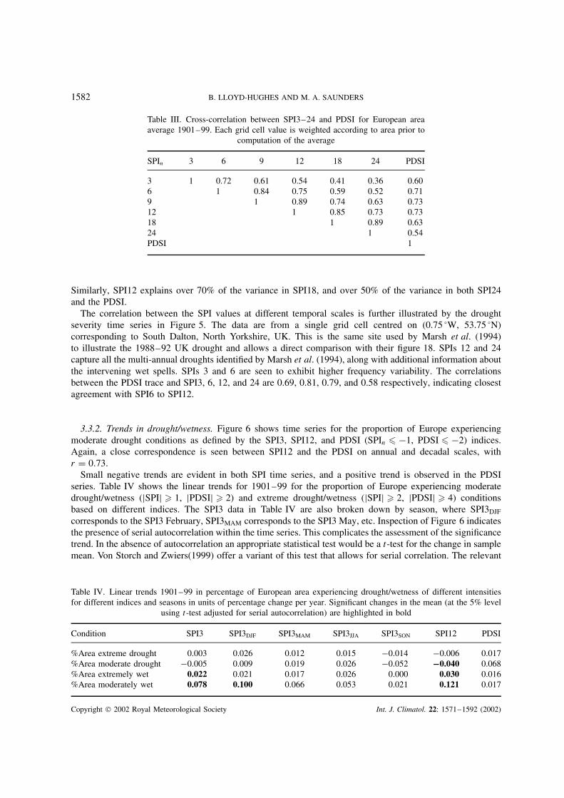
Table III. Cross-correlation between SPI3–24 and PDSI for European areaaverage 1901–99. Each grid cell value is weighted according to area prior to

computation of the average

SPIn 3 6 9 12 18 24 PDSI

3 1 0.72 0.61 0.54 0.41 0.36 0.606 1 0.84 0.75 0.59 0.52 0.719 1 0.89 0.74 0.63 0.7312 1 0.85 0.73 0.7318 1 0.89 0.6324 1 0.54PDSI 1

Similarly, SPI12 explains over 70% of the variance in SPI18, and over 50% of the variance in both SPI24and the PDSI.

The correlation between the SPI values at different temporal scales is further illustrated by the droughtseverity time series in Figure 5. The data are from a single grid cell centred on (0.75 °W, 53.75 °N)corresponding to South Dalton, North Yorkshire, UK. This is the same site used by Marsh et al. (1994)to illustrate the 1988–92 UK drought and allows a direct comparison with their figure 18. SPIs 12 and 24capture all the multi-annual droughts identified by Marsh et al. (1994), along with additional information aboutthe intervening wet spells. SPIs 3 and 6 are seen to exhibit higher frequency variability. The correlationsbetween the PDSI trace and SPI3, 6, 12, and 24 are 0.69, 0.81, 0.79, and 0.58 respectively, indicating closestagreement with SPI6 to SPI12.

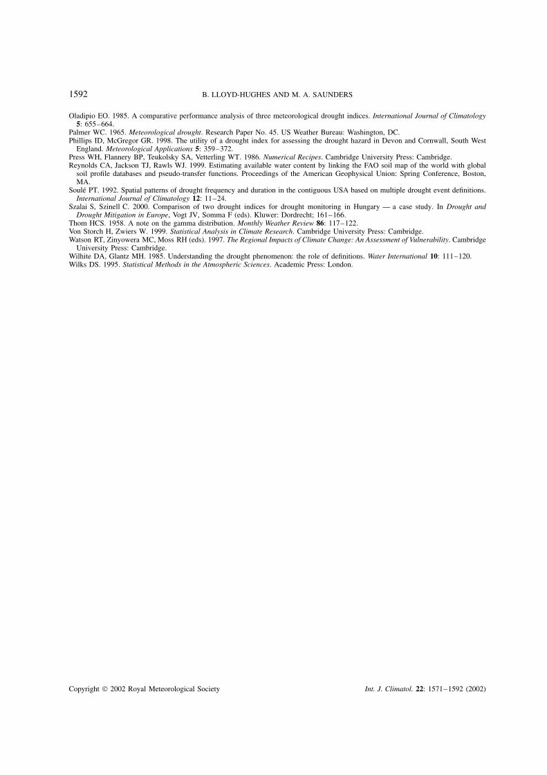
3.3.2. Trends in drought/wetness. Figure 6 shows time series for the proportion of Europe experiencingmoderate drought conditions as defined by the SPI3, SPI12, and PDSI (SPIn � −1, PDSI � −2) indices.Again, a close correspondence is seen between SPI12 and the PDSI on annual and decadal scales, withr = 0.73.

Small negative trends are evident in both SPI time series, and a positive trend is observed in the PDSIseries. Table IV shows the linear trends for 1901–99 for the proportion of Europe experiencing moderatedrought/wetness (|SPI| � 1, |PDSI| � 2) and extreme drought/wetness (|SPI| � 2, |PDSI| � 4) conditionsbased on different indices. The SPI3 data in Table IV are also broken down by season, where SPI3DJF

corresponds to the SPI3 February, SPI3MAM corresponds to the SPI3 May, etc. Inspection of Figure 6 indicatesthe presence of serial autocorrelation within the time series. This complicates the assessment of the significancetrend. In the absence of autocorrelation an appropriate statistical test would be a t-test for the change in samplemean. Von Storch and Zwiers(1999) offer a variant of this test that allows for serial correlation. The relevant

Table IV. Linear trends 1901–99 in percentage of European area experiencing drought/wetness of different intensitiesfor different indices and seasons in units of percentage change per year. Significant changes in the mean (at the 5% level

using t-test adjusted for serial autocorrelation) are highlighted in bold

Condition SPI3 SPI3DJF SPI3MAM SPI3JJA SPI3SON SPI12 PDSI

%Area extreme drought 0.003 0.026 0.012 0.015 −0.014 −0.006 0.017%Area moderate drought −0.005 0.009 0.019 0.026 −0.052 −0.040 0.068%Area extremely wet 0.022 0.021 0.017 0.026 0.000 0.030 0.016%Area moderately wet 0.078 0.100 0.066 0.053 0.021 0.121 0.017



SPI 3

1900 1925 1950 1975 2000

−2

0

2

SPI 6

1900 1925 1950 1975 2000

−2

0

2

SPI 12

1900 1925 1950 1975 2000

−2

0

2

SPI 24

1900 1925 1950 1975 2000

−2

0

2

PDSI

1900 1925 1950 1975 2000

−5

0

5

Figure 5. Drought severity index values representative of South Dalton, Yorkshire, UK, 1901–99. This site is selected for directcomparison with figure 18 of Marsh et al. 1994

statistic is

t ′ = µX − µY√s2X

n′X

+ s2Y

n′Y

(22)

where n′X and n′

Y represent estimates of the effective sample size, defined as

n′X = nX

1 +∑nX−1

k=1

(1 − k

nX

)ρX(k)

(23)



SPI 3

1900 1925 1950 1975 20000

20

40

60

%

Trend: −0.005 percent/yr +/− 0.021

SPI 12

1900 1925 1950 1975 20000

20

40

60

%

Trend: −0.040 percent/yr +/− 0.020

PDSI

1900 1925 1950 1975 20000

20

40

60

%

Trend: 0.068 percent/yr +/− 0.024

Figure 6. Proportion of Europe experiencing moderate drought conditions (SPIn �−1, PDSI �−2). The dashed lines show the lineartrend. Errors are ±2 standard errors in the gradient

and ρX(k) is the autocorrelation function

ρX(k) = 1

σ 2 Cov (Xi , Xi+k) (24)

and where X is the autocorrelated time series. For large samples (nX,Y > 30), t ′ follows the t-distribution.Linear trends that are significant at the 5% level after adjustment for serial autocorrelation are highlighted inbold in Table IV. The most significant trend is an increase in the percentage area experiencing moderatelywet conditions at the 12 month time scale. A significant positive trend is also evident in SPI3. Analysis ofthe seasonal values of SPI3 reveals the wetness trend to be strongest in the winter/spring and weakest insummer/autumn.



For drought, we conclude that the proportion of Europe experiencing extreme and/or moderate droughtconditions has changed insignificantly during the 20th century. Decadal trends in drought extent (Figure 6)are apparent, however, with greater pan-European drought incidence in the 1940s, early 1950s, and the 1990s,and lesser drought incidence in the 1910s, 1930s, and 1980s.

SPI 12

10°W 0 10°E 20°E 30°E

40°N

50°N

60°N

70°N

Trend (units/yr)

−0.01 0 0.01

PDSI

10°W 0 10°E 20°E 30°E

40°N

50°N

60°N

70°N

Trend (units/yr)

−0.02 0 0.02

(a)

(b)

Figure 7. Map of significant linear trend 1901–99 in (a) SPI12 and (b) PDSI at the 10% level adjusted for autocorrelation



3.3.3. Spatial distribution of trend. Figure 7 illustrates the spatial distribution of linear trend in the valuesof (a) SPI12 and (b) the PDSI (filtered for significance at the 10% level after adjustment for temporalautocorrelation) for the period 1901–99. Spatial variation is evident across Europe. Significant positive trendsare seen in both indices over large parts of Scandinavia, the Netherlands and the Ukraine. In contrast, areasof eastern Europe and western Russia have become drier during the 20th century. The pattern correlationbetween panels (a) and (b) is 0.82. Seasonal maps of SPI3 (not shown) for winter show similar trends andpatterns to those observed in SPI12. Weaker, less distinct spatial differences in trend are seen in spring andautumn. Virtually no significant trends are detected during the summer.

3.3.4. Number of drought events. Figure 8 maps the number of extreme drought events (SPIn � −2,PDSI � −4) by grid cell across Europe for 1901–99 computed from (a) SPI12 and (b) PDSI. Individualevents are defined by zero crossings that bound the exceedance. The figure shows that the mean numberof events is similar for both indices, but that the number of extreme droughts computed from the PDSI ismore variable, i.e. the PDSI shows a greater range of values. Extreme droughts classified by the PDSI occurwith a greater frequency over central and eastern Europe, and with a lower frequency along much of thenorthwestern seaboard, the Mediterranean seaboard, and the Alps. The spatial distribution of extreme droughtfrequencies for SPI12 is more homogeneous. Similarities do exist between Figure 8(a) and (b), for exampleover Italy and the Alps, but the overall agreement is poor, with a pattern correlation coefficient of just 0.25.

Table V lists the average number of exceedances by grid cell for extreme (|SPIn| � 2, |PDSI| � 4) andmoderate (|SPIn| � 1, |PDSI| � 2) drought/wetness events for the period 1901–99. The data are furtherdivided into two splits: 1901–50 and 1951–99. The mean number by grid cell of extreme and moderateEuropean drought events, on a time scale of 12 months, is 6 ± 2 and 23 ± 3 events respectively during the20th century. The mean number of droughts in each 50 year split is almost identical. In contrast, the meannumber of extreme and moderate wet events have tended to increase from 1901–50 to 1951–99 (Table V).

3.3.5. Mean duration of droughts. A similar mapping, this time of the mean duration of extreme droughts,is shown in Figure 9. Structure is again visible within the plots, but this time there is more agreement betweenthe PDSI and SPI12 classifications (r = 0.45). The longest mean extreme drought durations are found in Italy,northwest France, Finland, and northwest Russia. The clustering in these regions reflects spatial autocorrelationbetween neighbouring grid cells. Comparing Figure 9 with Figure 8 shows a tendency (in both the SPI12 andPDSI classifications) for regions of higher (lower) mean extreme drought duration to correspond to regions oflower (higher) mean drought number. Thus, where extreme droughts are more common their duration tendsto be shorter, and vice versa.

Table V. Mean number of extreme (|SPIn| � 2, |PDSI| � 4) and moderate (|SPIn| � 1, |PDSI| � 2) drought/wet eventsacross Europe for the periods 1901–99, 1901–50, and 1951–99. The duration of an event is defined as the time between

the zero crossings that bound the event. Standard deviations are given in parentheses

Condition SPI3 SPI6 SPI9 SPI12 SPI18 SPI24 PDSI

Extreme drought 1901–99 20(4) 12(3) 9(2) 6(2) 5(2) 3(1) 8(3)1901–50 10(4) 6(2) 5(2) 3(2) 3(1) 2(1) 4(2)1951–99 10(3) 6(2) 4(2) 3(2) 2(1) 1(1) 4(2)

Moderate drought 1901–99 68(6) 41(4) 30(4) 23(3) 16(3) 12(3) 26(4)1901–50 34(5) 21(3) 15(3) 12(2) 9(2) 7(2) 12(3)1951–99 34(5) 20(4) 14(3) 11(3) 8(2) 6(2) 14(3)

Extremely wet 1901–99 15(3) 10(2) 7(2) 6(2) 4(1) 4(1) 9(2)1901–50 6(3) 4(2) 3(2) 2(1) 2(1) 1(1) 4(2)1951–99 9(3) 6(2) 5(2) 4(1) 3(1) 2(1) 5(2)

Moderately wet 1901–99 65(6) 39(4) 28(4) 21(3) 15(3) 12(2) 28(4)1901–50 30(5) 18(4) 12(3) 9(3) 7(2) 5(2) 13(3)1951–99 35(4) 22(3) 16(3) 12(2) 9(2) 7(2) 15(3)



SPI 12

10°W 0 10°E 20°E 30°E

40°N

50°N

60°N

70°N

Number of exceedances

4 8 12

PDSI

10°W 0 10°E 20°E 30°E

40°N

50°N

60°N

70°N

Number of exceedances

4 8 12

(a)

(b)

Figure 8. Number of extreme drought events (SPIn �−2, PDSI �−4) by grid cell for Europe 1901–99 based on (a) SPI12 and (b)PDSI. Individual events are defined by the zero crossings that bound the exceedance

Table VI lists the mean duration by grid cell of extreme and moderate drought/wetness events acrossEurope. Durations are computed for the periods 1901–99, 1901–50, and 1951–99. Each grid cell is againweighted according to its area. The mean duration of extreme and moderate European drought events, on atime scale of 12 months, is 27 ± 8 months and 21 ± 3 months respectively. There is an indication that themean duration has shortened during the 20th century. Comparison of the SPI and the PDSI index results



SPI 12

10°W 0 10°E 20°E 30°E

40°N

50°N

60°N

70°N

Mean duration (months)

20 30 40

PDSI

10°W 0 10°E 20°E 30°E

40°N

50°N

60°N

70°N

Mean duration (months)

20 30 40

(b)

(a)

Figure 9. Mean duration of extreme drought events (SPIn �−2, PDSI �−4) by grid cell for Europe 1901–99 for (a) SPI12 and (b)PDSI. Individual events are defined by the zero crossings that bound the exceedance

indicates best agreement with SPI12 for extreme drought durations and SPI9 for moderate drought durations.SPI3 drought durations are least variable, and last typically 6 to 8 months. The mean wetness durations inTable VI suggest a lengthening has occurred during the 20th century.

The mean durations computed for the splits in Table VI are systematically lower than those calculatedfrom the full record. This is an artefact of the splitting process, since single events in the full record that



Table VI. Mean duration of extreme (|SPIn| � 2, |PDSI| � 4) and moderate (|SPIn| � 1, |PDSI| � 2) drought/wet eventsacross Europe for the periods 1901–99, 1901–50, and 1951–99. The duration of an event is defined as the time between

the zero crossings that bound the event. Standard deviations are given in parentheses


Extreme drought 1901–99 8(1) 14(2) 20(4) 27(8) 40(15) 55(26) 28(8)1901–50 8(2) 15(4) 21(7) 28(11) 39(20) 51(34) 29(14)1951–99 7(2) 13(3) 18(6) 23(10) 30(17) 36(26) 24(10)


Extremely wet 1901–99 8(1) 14(3) 21(4) 28(6) 38(11) 50(17) 25(7)1901–50 8(2) 14(5) 19(8) 23(12) 29(19) 34(26) 27(12)1951–99 8(2) 14(4) 20(6) 27(10) 37(16) 48(25) 23(9)

Moderately wet 1901–99 7(1) 12(1) 16(2) 21(3) 29(5) 38(8) 16(3)1901–50 7(1) 11(2) 16(3) 20(4) 28(7) 35(11) 17(5)1951–99 8(1) 12(2) 17(3) 22(5) 30(8) 39(11) 15(5)

extend through 1950–51 will be counted separately as two short events in the splits. The bias becomes moreapparent when considering longer period events and extremes.

3.3.6. Maximum duration of droughts. Maps of the duration of the longest extreme drought for the period1901–99 for a given grid cell (not shown) bear a close resemblance to those shown in Figure 9. This impliesthat the mean durations may be dominated by a few particularly long events.

Table VII lists the maximum duration by grid cell of extreme and moderate drought/wetness events acrossEurope. Durations are shown for 1901–99, 1901–50, and 1951–99. The mean maximum duration of extremeand moderate droughts, on a time scale of 12 months, is 48 ± 17 months and 56 ± 18 months respectively.Other findings parallel those for the mean duration of drought/wetness events (Section 3.3.5).

Table VII. Maximum duration of extreme (|SPIn| � 2, |PDSI| � 4) and moderate (|SPIn| � 1, |PDSI| � 2) drought/wetevents across Europe for the periods 1901–99, 1901–50, and 1951–99. The duration of an event is defined as the time

between the zero crossings that bound the event. Standard deviations are given in parentheses


Extreme drought 1901–99 20(6) 30(10) 39(13) 48(17) 63(26) 79(37) 57(23)1901–50 18(7) 26(11) 34(15) 41(19) 52(30) 64(43) 47(25)1951–99 15(5) 22(8) 27(12) 32(16) 38(23) 42(31) 40(19)


Extremely wet 1901–99 19(6) 28(8) 36(12) 46(16) 60(23) 72(29) 55(20)1901–50 14(5) 20(9) 25(12) 28(16) 34(23) 38(31) 44(30)1951–99 17(6) 25(9) 32(13) 40(18) 52(25) 63(34) 42(19)

Moderately wet 1901–99 30(10) 37(11) 46(14) 56(17) 71(23) 86(29) 57(19)1901–50 22(8) 28(9) 34(12) 40(14) 49(20) 59(25) 48(21)1951–99 26(10) 33(12) 41(15) 50(18) 64(24) 78(31) 44(17)



4. DISCUSSION

The gamma distribution provided the best fit of the models tested for describing monthly precipitation acrossEurope. The improvement in fit achieved by the gamma distribution over the normal is greatest for arid regionsat short time scales. None of the distributions tested could adequately model precipitation over eastern Turkeyor northwest Spain. This was true for all months and for all time scales. An improved fit for these regionscould be achieved using a theoretical model with a narrow peak and long tails, such as the Cauchy distribution.However, it is unlikely that such a model would perform well outside of these regions. Given the relativelysmall fraction of the data that are invalid (6–15% of the study area), it seemed reasonable to simply excludethe invalid data from the rest of the analysis. Future work may lead to a multi-model scheme wherebyprecipitation data are standardized through transformation of the theoretical distribution that provides thebest fit.

Trends in drought/wetness, though small for Europe as a whole, are significant over several Europeanregions. Upward trends in wetness are largest over northeast Europe during winter and spring. These resultsagree with the IPCC report findings on the regional impacts of climate change (Watson et al., 1997) whichshow a precipitation increase over the region from the Alps to northern Scandinavia since 1900. The dryingtendencies found in central eastern Europe and western Russia since 1900 are also in accord with the IPCCfindings.

Extreme droughts, as classified by the PDSI, occur with greater frequency over continental eastern Europe.Conversely, droughts are rarer along the northwest European seaboard, the Mediterranean seaboard, and theAlps. The SPI is found to be homogeneous with respect to the spatial distribution of extreme drought events.Hayes et al. (1999) cite the inability of the SPI to identify those regions that are more drought prone asa potential disadvantage. However, standardization in space and time is precisely what is required from astandard classification scheme where the frequency of a given event should be independent of location. Thus,the SPI should be viewed as superior to the PDSI for classifying droughts on a standard consistent scale.Apart from the spatial distribution of drought incidence, the SPI12 index yields results nearly identical tothose obtained using the PDSI. This agrees with Oladipio (1985), who, using data for Nebraska, showedthat indices based solely on precipitation can perform well when compared with more complex hydrologicalindices such as the PDSI. The SPI has the additional advantage of a variable time scale, which can benefitinvestigations of the temporal evolution of particular events (e.g. the US 1996 drought (Hayes et al., 1999)).

5. CONCLUSIONS

We have presented a new high spatial resolution, multi-temporal climatology for the incidence of 20th centuryEuropean drought. The climatology is based on monthly SPIs calculated on a 0.5 °grid across the whole ofEurope for the period 1901–99.

The gamma distribution has been found to provide the best model for describing monthly precipitation overmost of Europe. Notable exceptions occur in northwest Spain and eastern Turkey, where the equiprobabilitytransform of the data into the standardized normal distribution fails and the resultant SPI values are invalid.Given the small fraction of the data that are invalid (6–15% of the study area), no attempt has been made tostandardize the data by other means. Invalid data have simply been excluded from the analysis.

We have compared characteristics of the SPI computed over time scales of 3 to 24 months with the PDSI.In general, SPI12 exhibits a close correspondence to the PDSI. This agrees with the findings of previousstudies, e.g. Guttman (1998) for the USA, and Bussay et al. (1998) for Hungary. It is clear that much of thevariability seen in the PDSI results directly from precipitation.

Trends in SPI and PDSI values indicate that the proportion of Europe experiencing extreme and/or moderatedrought conditions has changed insignificantly during the 20th century. Spatially, changes in the mean valueof both indices are found to be variable, with a significant shift towards wetter conditions observed overnortheast Europe. Drying tendencies are observed over central eastern Europe and western Russia. Trends arestrongest in winter/spring and weakest in the summer/autumn.



Analysis of extreme drought events shows the SPI provides a better spatial standardization than the PDSI.Extreme droughts, as classified by the PDSI, occur with a greater frequency within the interior of continentalEurope. Conversely, they are less common along the northwest European seaboard, the Mediterraneanseaboard, and the Alps. Extreme droughts, as classified by both the PDSI and SPI12, are found to persist onaverage for 2–3 years, with the most extreme droughts lasting in excess of 5 years. Regionally, the longestdroughts are found in Italy, northwest France, and northwest Russia, with typical durations of 40 months.

In summary, this paper has shown the SPI is a simple and effective tool for the study of European drought.A new high-resolution climatology of SPI values has been created and validated. We hope this climatologywill provide a useful resource for assessing European drought vulnerability on different spatial and temporalscales, and for initiating investigations into the seasonal predictability of European drought incidence.

ACKNOWLEDGEMENTS

Benjamin Lloyd-Hughes is supported by a Research Studentship from the UK Natural Environment ResearchCouncil. He gratefully thanks St. Paul Re. for industrial CASE sponsorship. We thank Richard Heim at NOAAfor supplying the code used to calculate the PDSI values. The CRU 0.5° lat/lon gridded monthly climate datawere supplied by the Climate Impacts LINK Project (UK Department of the Environment Contract EPG1/1/16) on behalf of the Climatic Research Unit, University of East Anglia, UK.

REFERENCES

Abramowitz M, Stegun A (eds). 1965. Handbook of Mathematical Formulas, Graphs, and Mathematical Tables. Dover Publications,Inc.: New York.

Alley WM. 1984. The Palmer drought severity index: limitations and assumptions. Journal of Climate and Applied Meteorology 23:1100–1109.

Briffa KR, Jones PD, Hulme M. 1994. Summer moisture variability across Europe, 1892–1991: an analysis based on the Palmer droughtseverity index. International Journal of Climatology 14: 475–506.

Bussay AM, Szinell C, Hayes M, Svoboda M. 1998. Monitoring drought in Hungary using the standardized precipitation index. AnnalesGeophysicae, Supplement 11 to Vol 16, the Abstract Book of 23rd EGS General Assembly, C450. April 1998, Nice; France.

Bussay A, Szinell C, Szentimery T. 1999. Investigation and Measurements of Droughts in Hungary. Hungarian Meteorological Service:Budapest.

Demuth S, Stahl K, (eds). 2001. Assessment of regional impact of droughts in Europe. Final report to the European Union ENV-CT97-00553. Institute of Hydrology, University of Freiburg: Freiburg, Germany.

Edwards DC, McKee TB. 1997. Characteristics of 20th century drought in the United States at multiple timescales. Colorado StateUniversity: Fort Collins. Climatology Report No. 97-2.

Estrela MJ, Penarrocha D, Millan M. 2000. Multi-annual drought episodes in the Mediterranean (Valencia region) from 1950–1996. Aspatio-temporal analysis. International Journal of Climatology 20: 1599–1618.

European Environment Agency. 2001. Sustainable water use in Europe, Part 3: extreme hydrological events: floods and droughts.Environmental Issue Report No. 21.

FAO. 1996. The Digitized Soil Map of the World Including Derived Soil Properties (CD-ROM). Food and Agriculture Organization:Rome.

Gibb O, Penman HL, Pereier HC, Ratcliffe RAS. 1978. Scientific Aspects of the 1975–76 Drought in England and Wales. The RoyalSociety: London.

Guttman NB. 1998. Comparing the Palmer drought severity index and the standardised precipitation index. Journal of the AmericanWater Resources Association 34: 113–121.

Hayes MJ, Svoboda MD, Wilhite DA, Vanyarkho OV. 1999. Monitoring the 1996 drought using the standardized precipitation index.Bulletin of the American Meteorological Society 80: 429–438.

Karl TR. 1983. Some spatial characteristics of drought duration in the United States. Journal of Climate and Applied Meteorology 22:1356–1366.

Kilsby CG (ed.). 2001. Water resources: influence of climate change in Europe ENV4-CT97-0452. Water Resource Systems ResearchLaboratory, University of Newcastle: Newcastle-Upon-Tyne, UK.

Lana X, Serra C, Burgueno A. 2001. Patterns of monthly rainfall shortage and excess in terms of the standardized precipitation index.International Journal of Climatology 21: 1669–1691.

Marsh TJ, Lees ML. 1985. The 1984 Drought. Institute of Hydrology: Wallingford, UK.Marsh TJ, Monkhouse RA, Arnell NW, Lees ML, Reynard NS. 1994. The 1988–92 Drought. Institute of Hydrology: Wallingford, UK.McKee TB, Doesken NJ, Kliest J. 1993. The relationship of drought frequency and duration to time scales. In Proceedings of the 8th

Conference on Applied Climatology, 17–22 January, Anaheim, CA. American Meteorological Society: Boston, MA; 179–184.New M, Hulme M, Jones P. 2000. Representing twentieth-century space–time climate variability, part II: development of 1901–96

monthly grids of terrestrial surface climate. Journal of Climate 13: 2217–2238.Nigam S, Barlow M, Berbery EH. 1999. Analysis links Pacific decadal variability to drought and streamflow in United States. EOS

Transactions of the American Geophysical Union 80: 621–625.



Oladipio EO. 1985. A comparative performance analysis of three meteorological drought indices. International Journal of Climatology5: 655–664.

Palmer WC. 1965. Meteorological drought. Research Paper No. 45. US Weather Bureau: Washington, DC.Phillips ID, McGregor GR. 1998. The utility of a drought index for assessing the drought hazard in Devon and Cornwall, South West

England. Meteorological Applications 5: 359–372.Press WH, Flannery BP, Teukolsky SA, Vetterling WT. 1986. Numerical Recipes. Cambridge University Press: Cambridge.Reynolds CA, Jackson TJ, Rawls WJ. 1999. Estimating available water content by linking the FAO soil map of the world with global

soil profile databases and pseudo-transfer functions. Proceedings of the American Geophysical Union: Spring Conference, Boston,MA.

Soule PT. 1992. Spatial patterns of drought frequency and duration in the contiguous USA based on multiple drought event definitions.International Journal of Climatology 12: 11–24.

Szalai S, Szinell C. 2000. Comparison of two drought indices for drought monitoring in Hungary — a case study. In Drought andDrought Mitigation in Europe, Vogt JV, Somma F (eds). Kluwer: Dordrecht; 161–166.

Thom HCS. 1958. A note on the gamma distribution. Monthly Weather Review 86: 117–122.Von Storch H, Zwiers W. 1999. Statistical Analysis in Climate Research. Cambridge University Press: Cambridge.Watson RT, Zinyowera MC, Moss RH (eds). 1997. The Regional Impacts of Climate Change: An Assessment of Vulnerability. Cambridge

University Press: Cambridge.Wilhite DA, Glantz MH. 1985. Understanding the drought phenomenon: the role of definitions. Water International 10: 111–120.Wilks DS. 1995. Statistical Methods in the Atmospheric Sciences. Academic Press: London.


A drought climatology for Europe

Documents

Transcript of A drought climatology for Europe