Finite volume methods for balance laws withspatially-varying flux functions

Marek Brandner, Stanislav Mıka ∗

1 June 2003

Abstract

In this paper we study numerical methods to solve non-autonomous conservationlaws of the form qt + [f(q, x)]x = 0. We give a survey of schemes used to solve somespecial cases of conservation laws of this type. Furthemore, we study two approachesto solve the conservation laws with spatially-varying flux functions in the generalform.

Keywords: finite volume methods, upwind schemes, central schemes, advection equation, fluidflow through the male urethra

AMS subject classification: 76T05, 65M05, 76D05

1 Strictly hyperbolic problems

In this section we give a short survey of basic facts for strictly hyperbolic conservationlaws.

1.1 Scalar conservation laws

We consider non-linear conservation law in the standard (autonomous) form

ut + [f(u)]x = 0, x ∈ R, t ∈ (0, T )u(x, 0) = u0(x), x ∈ R,

(1)

where f ∈ C2(R) and u0 ∈ BV (R).

∗Centre of Applied Mathematics, Department of Mathematics, University of West Bohemia, Pilsen

1

Definition. Let u0(x) ∈ L1,loc(R) and the function f = f(u) is Lipschitz continuous.Any function u(x, t) ∈ L∞loc(R× (0,∞)) that fulfils

∞∫

0

∞∫

−∞[φtu + φxf(u)] dx dt = −

∞∫

−∞φ(x, 0)u0(x) dx (2)

for all φ ∈ C10(R×R) is called the weak solution of (1). C1

0(R×R) is the set of continuouslydifferentiable functions φ = φ(x, t) where

supp φ =(x, t) ∈ R2 : φ(x, t) 6= 0

is bounded.

Example.

ut + (u3)x = 0, u(x, 0) =

uL if x < 0uR if x > 0

0 0.1 0.2 0.3 0.4 0.5 0.6 0.7 0.8 0.9 1−1

−0.8

−0.6

−0.4

−0.2

0

0.2

0.4

0.6

0.8

1

initial conditionupwind method

0 0.1 0.2 0.3 0.4 0.5 0.6 0.7 0.8 0.9 1−1.5

−1

−0.5

0

0.5

1

initial conditionBeam−Warming

0 0.1 0.2 0.3 0.4 0.5 0.6 0.7 0.8 0.9 1−1

−0.8

−0.6

−0.4

−0.2

0

0.2

0.4

0.6

0.8

1

initial conditionBeam−Warming

Figure 1: uL = 1, uR = −1 Figure 2: uL = 1, uR = −1.2 Figure 3: uL = 1, uR = −0.4T = 0.15 T = 0.15 T = 0.5

We can obtain three types of weak solutions for the previous conservation law. The firstone is the compound wave — the shock wave with the attached rarefaction1, the secondone is the slow non-classical shock followed by the rarefaction and third one is the slownon-classical shock followed by the fast classical shock2.

Definition. Let uε is the solution of the initial value problem

ut + [f(u)]x = εuxx, x ∈ R, 0 < t < T, ε > 0

u(x, 0) = u0(x), x ∈ R.(3)

1The solution is computed by the first-order upwind method(h = 0.01, τ = h/100).2These two solutions are computed by the second-order Beam-Warming scheme(h = 0.01, τ = h/100).

2

If the limitu∗ = lim

ε→0u(ε), (4)

exists, it is called the vanishing viscosity solution of (1).

The solution in Fig. 1 is the vanishing viscosity solution, the other two are also limitingsolutions. However, the equation with the artificial viscosity (or diffusion) (3) is replaced bya viscosity-dispersion equation (see []). To distinguish which weak solution is a vanishing-viscosity solution we introduce entropy conditions (see []).

1.2 Systems of conservation laws

We consider the system of conservation laws

ut + [f(u)]x = 0, x ∈ R, t ∈ (0, T )u(x, 0) = u0(x), x ∈ R,

(5)

where u0 = u0(x) : R → Rm, f = f(u) : Rm → Rm is sufficiently smooth. The weakand vanishing-viscosity solutions are defined by the same way as in the scalar case. Thissystem can be rewritten to the form

ut + A(u)ux = 0, x ∈ R, t ∈ (0, T )u(x, 0) = u0(x), x ∈ R,

(6)

where A(u) = ∂f∂u

is the Jacobi matrix of the function f = f(u). This system is said to behyperbolic if A is diagonizable with real eigenvalues λi(u), i. e., a regular matrix R = R(u)exists for all u that

Λ(u) = [R(u)]−1A(u)R(u),

where Λ(u) is a diagonal matrix. If the eigenvalues λi(u) are distinct then (5) is called thestrict hyperbolic system. We distinguish two cases:

• ∇λi(u) · ri(u) ≡ 0 ∀u (linear degeneracy),

• ∇λi(u) · ri(u) 6= 0 ∀u (genuine non-linearity).

The linearly degenerate case generates a contact discontinuity, the genuinely non-linearcase generates either a shock or a rarefaction wave. The system is said to be weaklyhyperbolic if A has real eigenvalues λi(u) and it is not diagonizable.

3

2 Finite volume schemes

We discretize the space-time domain by choosing a mesh sizes h and a time step τ anddefine the discrete mesh points (xj, tn) by

xj = jh, j = 0,±1, . . . , tn = nτ, n = 0, 1, . . . , N.

For simplicity purposes we consider only the domain Ω = R×(0, T ) in what follows. In thiscase we have N = T/τ . Futhermore, we consider a uniform mesh, with h and τ constant,although the discussed methods can be extended to nonuniform meshes. The values of thetrue solution at the meshpoints are denoted by un

j = u(xj, tn). Our numerical methods willproduce approximations to un

j denoted by Unj . Futhermore we define

xj+1/2 = xj +h

2=

(j +

1

2

)h

and put Unj+1/2 ≈ u(xj+1/2, tn).

2.1 Autonomous case

We consider the difference schemes approximating the conservation law (5) in the conser-vative form

Un+1j = Un

j −τ

h

(Fn

j+1/2 − Fnj−1/2

). (7)

The function Fnj+1/2 is called the numerical flux.

We define the set of the Riemann problems for the linearized conservation laws

ut + Anj+1/2ux = 0, x ∈ R, t ∈ (tn, tn+1),

u(x, tn) =

Un

j , x < xj+1/2,Un

j+1, x > xj+1/2.(8)

where Anj+1/2 = A(Un

j ,Unj+1).

For the autonomous case f = f(u) the matrix A(U, U) has to fulfil three conditions

• the system (8) is strict hyperbolic,

• the matrix A(U, U) is the linearization of the f , i. e.,

f(U)− f(U) = A(U, U)(U− U) ∀U, U, (9)

• A → A(U), i e., A(U, U) → A(U) for U → U, U → U.

4

Then we can write

f(Unj+1)− f(Un

j ) = A(Unj ,U

nj+1)(U

nj+1 −Un

j ) (10)

and decompose the jump Unj+1 −Un

j on the right hand side by the following way

Unj+1 −Un

j =m∑

p=1

Υn,pj+1/2s

n,pj+1/2 =

m∑

p=1

wn,pj+1/2 (11)

where Υnj+1/2 = (Sn

j+1/2)−1(Un

j+1 − Unj ), sn,p

j+1/2 are the eigenvectors of A(Unj ,Un

j+1) (thecolumns of the matrix Sn

j+1/2). We obtain the decomposition

f(Unj+1)− f(Un

j ) = A(Unj ,U

nj+1)(U

nj+1 −Un

j ) =

= Snj+1/2Λ

nj+1/2(S

nj+1/2)

−1(Unj+1 −Un

j ) = Snj+1/2Λ

nj+1/2Υ

nj+1/2 =

=m∑

p=1Υn,p

j+1/2λn,pj+1/2s

n,pj+1/2.

(12)

The first-order upwind conservative scheme can be written in the form

Un+1j = Un

j −τ

h(Fn

j+1/2 − Fnj−1/2) (13)

where

Fnj+1/2 =

1

2[f(Un

j ) + f(Unj+1)]−

1

2|A(Un

j ,Unj+1)|(Un

j+1 −Unj ) (14)

and|A(Un

j ,Unj+1)| = Sn

j+1/2|Λnj+1/2|(Sn

j+1/2)−1. (15)

If we put (12) to (14) we obtain the following formula

Fnj+1/2 =

1

2[f(Un

j ) + f(Unj+1)]−

1

2

m∑

p=1

Υn,pj+1/2

∣∣∣λn,pj+1/2

∣∣∣ sn,pj+1/2. (16)

The wave-propagation algorithm is in the form

Un+1j = Un

j −τ

h[A+(∆Un

j−1/2) +A−(∆Unj+1/2)] (17)

where

A+(∆Unj−1/2) =

m∑

p=1

maxλn,pj−1/2, 0wn,p

j−1/2,

A−(∆Unj+1/2) =

m∑

p=1

minλn,pj+1/2, 0wn,p

j+1/2.

5

Remark In the case of the non-linear scalar conservation law

ut + [f(u)]x = 0 (18)

that can be rewritten in the form

ut + a(u)ux = 0, a(u) = fu,

we obtain the following algorithm

Un+1j = Un

j −τ

h(F n

j+1/2 − F nj−1/2) (19)

where

F nj+1/2 =

1

2[f(Un

j ) + f(Unj+1)]−

1

2|a(Un

j , Unj+1)|(Un

j+1 − Unj )

and

anj+1/2 = a(Un

j , Unj+1) =

f(Unj+1)− f(Un

j )

Unj+1 − Un

j

. (20)

The wave-propagation algorithm is in the form

Un+1j = Un

j −τ

h[A+(∆Un

j−1/2) +A−(∆Unj+1/2)]

whereA+(∆Un

j−1/2) = maxa(Unj−1, U

nj ), 0∆Un

j−1/2,

A−(∆Unj+1/2) = mina(Un

j , Unj+1), 0∆Un

j+1/2.

The high-resolution wave-propagation algorithm is in the form

Un+1j = Un

j −τ

h[A+(∆Un

j−1/2) +A−(∆Unj+1/2)]−

τ

h(Fn,H

j+1/2 − Fn,Hj−1/2), (21)

where

Fn,Hj+1/2 =

1

2

m∑

p=1

|λn,pj+1/2|(1−

τ

h|λn,p

j+1/2|)Υn,pj+1/2s

n,pj+1/2, (22)

Υn,pj+1/2 = Υn,p

j+1/2Ψ(Θn,pj+1/2), (23)

Θn,pj+1/2 =

Υn,pj−1/2

Υn,pj+1/2

if λn,pj+1/2 ≥ 0,

Υn,pj+3/2

Υn,pj+1/2

otherwise.(24)

The function Ψ = Ψ(Θ) is called the limiter. It can be defined by several ways, forexample

6

• Ψ(Θ) = minmod(1,Θ) (minmod limiter),

• Ψ(Θ) = max0, min1, 2Θ, min2,Θ (superbee limiter),

• Ψ(Θ) = max0, min1+Θ2

, 2, 2Θ (MC limiter),

• Ψ(Θ) = Θ+|Θ |1+|Θ | (van Leer limiter),

where

minmod(a, b) =

a if |a| < |b| and ab > 0,b if |b| < |a| and ab > 0,0 if ab ≤ 0.

2.2 Strictly hyperbolic systems with spatially-varying flux func-tions

Herein, we give some examples that are strictly hyperbolic and describe one approachto solve them (proposed by LeVeque in [BLMR02]). We will study strictly hyperbolicnon-autonomous system

qt + [f(q, x)]x = 0, x ∈ R, t > 0q(x, 0) = q0(x), x ∈ R.

(25)

2.2.1 Advection problem

We start with the very simple advection problem

qt + [a(x)q]x = 0, x ∈ R, t > 0, a(x) > 0 ∀x ∈ R,q(x, 0) = q0(x), x ∈ R,

(26)

where q = q(x, t) is the concentration of an agent driven with the velocity a = a(x). Wecan rewrite this advection problem to the form

qt + [g(q, x)]x = 0, x ∈ R, t > 0q(x, 0) = q0(x), x ∈ R,

(27)

where g(q, x) = a(x)q and also as the autonomous system for uknowns [q, w]T

qt + [wq]x = 0, x ∈ R, t > 0wt = 0, x ∈ R, t > 0

q(x, 0) = q0(x), x ∈ Rw(x, 0) = a(x), x ∈ R.

(28)

7

The Jacobi matrix

A(u) =

[a(x) q

0 0

].

of this system has two distinct eigenvalues λ1 = a(x) > 0 and λ2 = 0, i. e., it is strictlyhyperbolic.

We again consider the difference schemes approximating the conservation law in theconservative form

Qn+1j = Qn

j −τ

h

[Gn

j+1/2 −Gnj−1/2

]. (29)

On the time level n we replace the solution by the piecewise constant function Qn = Qn(x)

Qn(x) = Qnj for x ∈ (xj−1/2, xj+1/2).

We obtained the set of Riemann problems. Then the Riemann solution (the exact solutionof the Riemann problems) is

q∗(x, t) =

Qnj if x < xj+1/2

Qn,Rj if xj+1/2 < x < xj+1/2 + aj+1t

Qnj+1 if x > xj+1/2 + aj+1t

(30)

Towards computing Qn,Rj we use the fact that we expect the flux g = g(q(x, t), x) (g =

a(x)q(x, t)) to be continuous at the points x = xj+1/2, i. e., g(q(xj+1/2−, t), xj+1/2−) =

g(q(xj+1/2+, t), xj+1/2+) ∀t ∈ (tn, tn+1). Therefore, we obtain ajQnj = aj+1Q

n,Rj and Qn,R

j =

ajQnj /aj+1. The first-order upwind numerical flux has the form Gn

j+1/2 = g(Qn,Rj , xj+1) =

g(Qnj , xj). In the case of a non-autonomous equation (or a system) the solution has more

complicated structure. For example, the Riemann problem for the non-autonomous ad-vection equation (26) has the solution composed of contact discontinuities and stationarydiscontinuities.

2.2.2 Strictly hyperbolic system – flux-based wave decomposition

Now, we generalize the approach from the previous subsection. We consider the non-linearhyperbolic system of conservation laws in the form

qt + [g(q, x)]x = 0 (31)

where g = g(q, x) : Rm × R → Rm. We again define the set of the Riemann problems forthe linearized conservation laws

qt + Bnj+1/2qx = 0, x ∈ R, t ∈ (tn, tn+1),

q(x, tn) =

Qn

j , x < xj+1/2,Qn

j+1, x > xj+1/2.(32)

where Bnj+1/2 = B(Qn

j ,Qnj+1, xj, xj+1) is diagonizable.

8

Remark We assume that the initial value problem (32) is the linearization of the followingproblem

qt + [gj+1/2(q)]x = 0, x ∈ R, t ∈ (tn, tn+1),

gj+1/2(q) =

g(q, xj), x < xj+1/2,g(q, xj+1), x > xj+1/2.

(33)

In the non-autonomous case g = g(q, x) it is more convenient to use the decomposition (flux-based wave decomposition)

g(Qnj+1, xj+1)− g(Qn

j , xj) =m∑

p=1

Ξ n,pj+1/2r

n,pj+1/2 =

m∑

p=1

zn,pj+1/2 (34)

where Ξnj+1/2 = (Rn

j+1/2)−1[g(Qn

j+1, xj+1) − g(Qnj , xj)]. Herein, the matrix Rn

j+1/2 is com-

posed of the eigenvectors of the matrix B(Qnj ,Qn

j+1, xj, xj+1).

If we replace the condition (9) by

g(Qnj+1, xj+1)− g(Qn

j , xj) = B(Qnj ,Qn

j+1, xj, xj+1)(Qnj+1 −Qn

j ). (35)

we can write the formula

g(Qnj+1, xj+1)− g(Qn

j , xj) =m∑

p=1

Υn,pj+1/2λ

n,pj+1/2r

n,pj+1/2

where Υnj+1/2 = (Rn

j+1/2)−1(Qn

j+1 −Qnj ), i. e., Ξ n,p

j+1/2 = Υn,pj+1/2λ

n,pj+1/2.

The wave-propagation algorithm is in the form

Qn+1j = Qn

j −τ

h[B+(∆Qn

j−1/2) + B−(∆Qnj+1/2)] (36)

whereB+(∆Qn

j−1/2) =∑

λn,pj−1/2

>0

zn,pj−1/2,

B−(∆Qnj+1/2) =

∑

λn,pj+1/2

<0

zn,pj+1/2.

Remark In the case of the advection equation (26) we have m = 1, rn,1j+1/2 = 1. If we set

B(Qnj , Qn

j+1, xj, xj+1) = [g(q, x)]q|x=xj+1= aj+1 we obtain λn,1

j+1/2 = aj+1, g(Qnj+1, xj+1) −

g(Qnj , xj) = aj+1Q

nj+1 − ajQ

nj , zn,1

j+1/2 = vj+1Qnj+1 − vjQ

nj and (we don’t apply (35)!)

wn,1j+1/2 = Υn,1

j+1/2rn,1j+1/2 = zn,1

j+1/2/λn,1j+1/2 = Qn

j+1 − Qn,Rj 6= Qn

j+1 − Qnj . Futhermore, the

scheme described in this subsection is a generalization of the scheme (36).

9

2.2.3 Scalar conservation law – augmented formulation

We consider the initial value problem (26)

qt + [a(x)q]x = 0, x ∈ R, t > 0, a(x) > 0 ∀x ∈ R,q(x, 0) = q0(x), x ∈ R,

The general approach to solve the problems with spatially-varying flux function is basedon the solution of the augmented autonomous system. We rewrite the non-autonomousproblem above to the autonomous one (we add an appropriate degenerate conservationlaw) and obtain

ut + [f(u)]x = 0, x ∈ R, t > 0, u = [q, w]T , f = [wq, 0]T ,

[q(x, 0), w(x, 0)]T = [q0(x), a(x)]T , x ∈ R(37)

Then we apply the standard approach used in Sec. 2.1. The linearization of (26) is thestandard linearization (10) (described in 2.1) in the form

f(Unj+1)−f(Un

j ) = Anj+1/2(U

nj+1−Un

j ), Anj+1/2 =

[12(W n

j + W nj+1)

12(Qn

j + Qnj+1)

0 0

](38)

We can formulate the first-order upwind method in the form (13), (14) or (17). This schemecan be rewritten to the scalar form

Qn+1j = Qn

j − τh[Gn

j+1/2 −Gnj−1/2],

Gnj+1/2 = 1

2(W n

j Qnj + W n

j+1Qnj+1)− 1

2bnj+1/2(Q

nj+1 −Qn

j ),

bnj+1/2 = sign(W n

j + W nj+1)a

nj+1/2,

anj+1/2 =

W nj+1Qn

j+1−W nj Qn

j

Qnj+1−Qn

j, an

j+1/2 = 0 if Qnj+1 = Qn

j .

(39)

Futhermore, we will study the general initial value scalar problem in the form

qt + [g(q, x)]x = 0, x ∈ R, t > 0,q(x, 0) = q0(x), x ∈ R,

(40)

rewritten to the initial value vector problem

ut + [f(u)]x = 0, x ∈ R, t > 0, u = [q, w]T , f = [g(q, w), 0]T ,

[q(x, 0), w(x, 0)]T = [q0(x), x]T , x ∈ R.(41)

We can use the same approach as in the previous case and define the following linearization

f(Unj+1)− f(Un

j ) = Anj+1/2(U

nj+1 −Un

j ), Anj+1/2 =

[(a11)

nj+1/2 (a12)

nj+1/2

0 0

](42)

10

where

(a11)nj+1/2 =

1

2

[g(Qn

j+1, xj+1)− g(Qnj , xj+1)

Qnj+1 −Qn

j

+g(Qn

j+1, xj)− g(Qnj , xj)

Qnj+1 −Qn

j

],

(a12)nj+1/2 =

1

2

[g(Qn

j+1, xj+1)− g(Qnj+1, xj)

xj+1 − xj

+g(Qn

j , xj+1)− g(Qnj , xj)

xj+1 − xj

].

We can also formulate the upwind method in the form (13, 14) rewritten to the scalar form

Qn+1j = Qn

j − τh[Gn

j+1/2 −Gnj−1/2],

Gnj+1/2 = 1

2[g(Qn

j , xj) + g(Qnj+1, xj+1)]− 1

2bnj+1/2(Q

nj+1 −Qn

j ),

bnj+1/2 = sign[(a11)

nj+1/2]a

nj+1/2, an

j+1/2 =g(Qn

j+1,xj+1)−g(Qnj ,xj)

Qnj+1−Qn

j,

anj+1/2 = 0 if Qn

j+1 = Qnj

(43)

Remark In this case the condition (35)

g(Qnj+1, xj+1)− g(Qn

j , xj) = anj+1/2(Q

nj+1 −Qn

j )

holds. If we set λnj+1/2 = (a11)

nj+1/2 the scheme (43) is equivalent to (36).

2.2.4 System of conservation laws – augmented formulation

We can apply the same approach to the initial value problem for the system of conservationlaws in the form

qt + [g(q, x)]x = 0, x ∈ R, t > 0,q(x, 0) = q0(x), x ∈ R.

(44)

We rewrite this problem to

ut + [f(u)]x = 0, x ∈ R, t > 0, u = [qT , w]T, f = [gT (q, w), 0]

T,

[qT (x, 0), w(x, 0)]T

= [qT0 (x), x]

T, x ∈ R.

(45)

To be able to use the method based on the linearization (10)

f(Unj+1)− f(Un

j ) = Anj+1/2(U

nj+1 −Un

j )

where we have

f(Unj+1)− f(Un

j ) =

[g(Qn

j+1, xj+1)− g(Qnj , xj)

0

]

11

in the case (45), we have to find an appropriate matrix Anj+1/2 (the approximation of the

Jacobi matrix that fulfils three conditions (9)). We propose the following form

Anj+1/2 =

[(A11)

nj+1/2 (a12)

nj+1/2

0 0

](46)

where[A11(xj)]

nj+1/2(Q

nj+1 −Qn

j ) = g(Qnj+1, xj)− g(Qn

j , xj),

(A11)nj+1/2 =

1

2[A11(xj)]

nj+1/2 +

1

2[A11(xj+1)]

nj+1/2

(a12)nj+1/2 =

1

2

[g(Qn

j+1, xj+1)− g(Qnj+1, xj)

xj+1 − xj

+g(Qn

j , xj+1)− g(Qnj , xj)

xj+1 − xj

].

Remark (we drop the subscripts and superscripts below) If we are able to construct adiagonizable matrix A11 (i.e., A11S11 = S11Λ11) then we are also able to construct thediagonizable matrix An

j+1/2 (i.e., Anj+1/2S

nj+1/2 = Sn

j+1/2Λnj+1/2) in the form

[A11 a12

0 0

] [S11 −(A11)

−1a12

0 1

]=

[S11 −(A11)

−1a12

0 1

] [Λ11 00 0

].

The matrix S−1 has the form

S−1 =

[(S11)

−1 (S11)−1(A11)

−1a12

0 1

].

We use the fact that the matrix Anj+1/2 has the special form (46) and construct the first-

order upwind method (13, 16). We have

m+1∑

p=1

|λn,pj+1/2|Υn,p

j+1/2sn,pj+1/2 =

m∑p=1

|λn,pj+1/2|Υn,p

j+1/2(s11)n,pj+1/2

0

(47)

whereΥn

j+1/2 = (Snj+1/2)

−1(Unj+1 −Un

j ). (48)

If we set Ξ n,pj+1/2 = Υn,p

j+1/2λn,pj+1/2 we obtain

m∑p=1

|λn,pj+1/2|Υn,p

j+1/2(s11)n,pj+1/2 =

m∑p=1

sign(λn,pj+1/2)Ξ

n,pj+1/2(s11)

n,pj+1/2. (49)

We formulate the upwind method in the form (13, 14)

Qn+1j = Qn

j − τh[Gn

j+1/2 −Gnj−1/2],

Gnj+1/2 = 1

2[g(Qn

j , xj) + g(Qnj+1, xj+1)]−

−12

m∑p=1

sign(λn,pj+1/2)Ξ

n,pj+1/2(s11)

n,pj+1/2.

(50)

12

Remark In the case (40) we have

m∑p=1

sign(λn,pj+1/2)Ξ

n,pj+1/2(s11)

n,pj+1/2 = sign[(a11)

nj+1/2](a11)

nj+1/2

[1,

(a12)nj+1/2

(a11)nj+1/2

] [Qn

j+1 −Qnj

xj+1 − xj

]=

= sign[(a11)nj+1/2]

[g(Qn

j+1, xj+1)− g(Qnj , xj)

].

We obtained the first-order upwind method (43).

In the wave-propagation form it can be formulated as

Qn+1j = Qn

j − τh[A+(∆Qn

j−1/2) +A−(∆Qnj+1/2)],

A+(∆Qnj−1/2) =

∑

λn,pj−1/2

>0

Ξ n,pj−1/2(s11)

n,pj−1/2 =

∑

λn,pj−1/2

>0

zn,pj−1/2,

A−(∆Qnj+1/2) =

∑

λn,pj+1/2

<0

Ξ n,pj+1/2(s11)

n,pj+1/2 =

∑

λn,pj+1/2

<0

zn,pj+1/2.

(51)

The high-resolution wave-propagation algorithm is in the form

Qn+1j = Qn

j −τ

h[A+(∆Qn

j−1/2) +A−(∆Qnj+1/2)]−

τ

h(Gn,H

j+1/2 −Gn,Hj−1/2), (52)

where

Gn,Hj+1/2 =

1

2

m∑

p=1

|λn,pj+1/2|(1−

τ

h|λn,p

j+1/2|)Υn,pj+1/2(s11)

n,pj+1/2, (53)

Υn,pj+1/2 = Υn,p

j+1/2Ψ(Θn,pj+1/2), (54)

Θn,pj+1/2 =

Υn,pj−1/2

Υn,pj+1/2

if λn,pj+1/2 ≥ 0,

Υn,pj+3/2

Υn,pj+1/2

otherwise.(55)

Remark In the case (40) we have

Gn,Hj+1/2 = 1

2sign

[(a11)

nj+1/2

] (1− τ

h|(a11)

nj+1/2|

)(a11)

nj+1/2Υ

nj+1/2(s11)

nj+1/2 =

= 12sign

[(a11)

nj+1/2

] (1− τ

h|(a11)

nj+1/2|

)(a11)

nj+1/2Υ

nj+1/2Ψ(Θn

j+1/2) =

= 12sign

[(a11)

nj+1/2

] (1− τ

h|(a11)

nj+1/2|

) [g(Qn

j+1, xj+1)− g(Qnj , xj)

]Ψ(Θn

j+1/2).

13

2.3 Non-strictly hyperbolic systems with spatially-varying fluxfunctions

In this section we study schemes for non-strictly hyperbolic systems. First, we describesome approaches for the advection equation and after that we generalize them to solvegeneral problems.

2.3.1 Generalized advection problem

We consider the initial value problem in the form

qt + [a(x)φ(q)]x = 0, x ∈ R, t > 0q(x, 0) = q0(x), x ∈ R.

(56)

This system can be rewritten to

qt + [wφ(q)]x = 0, x ∈ R, t > 0wt = 0, x ∈ R, t > 0

q(x, 0) = q0(x), x ∈ R,w(x, 0) = a(x), x ∈ R.

(57)

The eigenvalues of the Jacobi matrix of this system are λ1 = a(x)φq, λ2 = 0. If w = 0 thesystem is not strictly hyperbolic (even if φ = φ(q) is convex, i. e., φq is monotone). Towersproposed in [] the scheme

Qn+1j = Qn

j −τ

h[An

j+1/2Φnj+1/2 − An

j−1/2Φnj−1/2] (58)

where

Φnj+1/2 =

Φ(Qn

j+1, Qnj ) if An

j+1/2 ≥ 0

Φ(Qnj , Q

nj+1) if An

j+1/2 < 0Φ(a, b) =

min〈a,b〉

φ(q) if a ≤ b

max〈b,a〉

φ(q) if a > b(59)

Definition.

1. The conservative scheme in the form

Qn+1j = Qn

j −τ

h[Gn

j+1/2 −Gnj−1/2] (60)

is called monotone if the condition

(Qnj ≤ Qn

j ) =⇒ (Qn+1j ≤ Qn+1

j ) ∀j

is fulfiled for all approximate solutions Qnj and Qn

j .

14

2. The scheme (60) is called sign preserving if the condition

Qnj ≥ 0 =⇒ Qn+1

j ≥ 0 ∀j and n = 0, 1, . . . , N

is fulfiled.

3. The scheme (60) is called TVD (total variation diminishing) if the condition

TV(Qn+1) ≤ TV(Qn) ∀n,

whereTV(Qn) =

∑

j

|Qnj+1 −Qn

j |,

is fulfiled.

Theorem. If τh‖a‖∞‖φq‖∞ ≤ 1

2(where ‖a‖∞ = max

x|a(x)|) holds then the scheme (58)

is monotone.

Theorem. Let φ(q) = q. The scheme (58) is sign preserving provided that

‖a‖∞ τ

h≤ 1

2. (61)

Proof The scheme (58) can be rewritten in the form

Qn+1j = Qn

j − τh[12V n

j+1/2(Qnj + Qn

j+1)− 12|V n

j+1/2|(Qnj+1 −Qn

j )]+

+ τh[12V n

j−1/2(Qnj−1 + Qn

j )− 12|V n

j−1/2|(Qnj −Qn

j−1)].(62)

Then we can write

Qn+1j = Qn

j [1− τ2h

V nj+1/2 − τ

2h|V n

j+1/2| − τ2h

V nj−1/2 + τ

2h|V n

j−1/2|]−− τ

2h(V n

j+1/2 − |V nj+1/2|)Qn

j+1 + τ2h

(V nj−1/2 + |V n

j−1/2|)Qnj−1.

(63)

Futhermore, we consider the scheme

Qn+1j = Qn

j −τ

h(Gn

j+1/2 −Gnj−1/2) (64)

where

Gnj+1/2 =

1

2[vjφ(Qn

j ) + vj+1φ(Qnj+1)]−

1

2|an

j+1/2|(Qnj+1 −Qn

j ) (65)

and

anj+1/2 =

vj+1φ(Qnj+1)−vjφ(Qn

j )

Qnj+1−Qn

j, if Qn

j+1 6= Qnj

[v(x)φq]xj+1/2,tnotherwise.

15

If τh|an

j+1/2| ≤ 1 ∀n, j then the scheme is TVD. If we achieve this condition it can leadto slow-down or to abort the computation because the time step τ can tend to zero. (Inthe autonomous case (18) we have the different situation: There is possible to bound|an

j+1/2| by the maximum of fu(u).) It is induced by the fact that the exact solution ofthe non-autonomous problem is not TVD generally. This scheme is not above monotone.To achieve an entropy-satisfying solution we have to use an entropy fix procedure in thetransonic case.

If we want to use upwind schemes described in Sec. 2.2.4 we have to modify theevaluation of the numerical fluxes. The first possibility is locally to use the numericalflux generated by a central scheme described below or to use the wave propagation formand modify the computation of A−(∆Qn

j+1/2) and A+(∆Qnj+1/2) (to insert the weakly

hyperbolic case here).

2.3.2 Central schemes

The other possibility is to use a central scheme. By this way we circumvent the problem ofthe construction of the Riemann solver. We present here the second order central scheme(Tadmor, Nessyahu). This is the two-step predictor-corrector-type procedure:

Qn+1/2j = Qn

j − 12

τh(g′)n

j ,

(Q′)nj = MM

(2∆Qn

j+1/2,12(Qn

j+1 −Qnj−1), 2∆Qn

j−1/2

),

(g′)nj = MM

(2∆gn

j+1/2,12

[g(Qn

j+1, xj+1)− g(Qnj−1, xj−1)

], 2∆gn

j−1/2

),

∆Qnj+1/2 = Qn

j+1 −Qnj , ∆gn

j+1/2 = g(Qnj+1, xj+1)− g(Qn

j , xj),

(66)

MM(b1,b2, . . .) =

MM ((b1)1, (b2)1, . . .)MM ((b1)2, (b2)2, . . .)

· · ·MM ((b1)m, (b2)m, . . .)

MM(b1, b2, . . .) =

minkbk bk > 0 ∀k,

maxkbk bk < 0 ∀k,

0 otherwise,

(67)

Qn+1j+1/2 =

1

2(Qn

j + Qnj+1) +

1

8[(Q′)n

j − (Q′)nj+1]−

τ

h[g(Q

n+1/2j+1 )− g(Q

n+1/2j )] (68)

Remark We use the semidiscrete high-resolution schemes in our numerical experiments(because they are - for example - more convenient for steady-state computations).

16

0 20 40 60 80 100 120 140 160 180 2000.1

0.15

0.2

0.25

0.3

0.35

0.4

0.45the first−order scheme with the entropy fixthe upwind scheme (64)high−resolutionscheme without an entropy fix

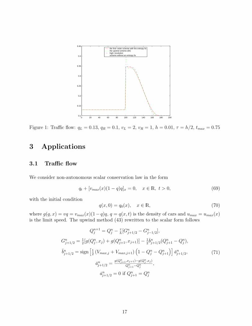
Figure 1: Traffic flow: qL = 0.13, qR = 0.1, vL = 2, vR = 1, h = 0.01, τ = h/2, tmax = 0.75

3 Applications

3.1 Traffic flow

We consider non-autonomous scalar conservation law in the form

qt + [vmax(x)(1− q)q]x = 0, x ∈ R, t > 0, (69)

with the initial conditionq(x, 0) = q0(x), x ∈ R, (70)

where g(q, x) = vq = vmax(x)(1− q)q, q = q(x, t) is the density of cars and umax = umax(x)is the limit speed. The upwind method (43) rewritten to the scalar form follows

Qn+1j = Qn

j − τh[Gn

j+1/2 −Gnj−1/2],

Gnj+1/2 = 1

2[g(Qn

j , xj) + g(Qnj+1, xj+1)]− 1

2bnj+1/2(Q

nj+1 −Qn

j ),

bnj+1/2 = sign

[12(Vmax,j + Vmax,j+1)

(1−Qn

j −Qnj+1

)]an

j+1/2,

anj+1/2 =

g(Qnj+1,xj+1)−g(Qn

j ,xj)

Qnj+1−Qn

j,

anj+1/2 = 0 if Qn

j+1 = Qnj

(71)

17

3.2 River flow

We consider non-autonomous scalar conservation law in the form

φt + qx = 0, x ∈ R, t > 0, (72)

with the initial conditionφ(x, 0) = φ0(x), x ∈ R, (73)

where q = q(φ, x) =(

gψ

)sin(α(x))φ5/4 is the flow rate, φ = φ(x, t) is the cross-section of

the stream bed, g is the gravity acceleration, ψ is the friction factor and α = α(x) is thedownstream slope.

Remark We suppose that a force balance gives

lτs = %gφ sin(α)

where τs is the shear stress given by the friction law

τs = f%v2.

The velocity v = v(x, t) of the flow is given by

v =q

φ.

The upwind method (43) rewritten to the scalar form follows

An+1j = An

j − τh[Gn

j+1/2 −Gnj−1/2],

Gnj+1/2 = 1

2[g(An

j , xj) + g(Anj+1, xj+1)]− 1

2bnj+1/2(A

nj+1 − An

j ),

bnj+1/2 = sign

[λn

j+1/2

]an

j+1/2,

anj+1/2 =

g(Anj+1,xj+1)−g(An

j ,xj)

Anj+1−An

j,

anj+1/2 = 0 if An

j+1 = Anj ,

λnj+1/2 = 1

2

(gψ

)1/2 [√sin(xj) +

√sin(xj+1)

]·

·Anj +(An

j )3/4(Anj+1)

1/4+(Anj )1/2(An

j+1)1/2+(An

j )1/4(Anj+1)

3/4+Anj+1

(Anj )3/4+(An

j )1/2(Anj+1)

1/4+(Anj )1/4(An

j+1)1/2+(An

j+1)3/4

(74)

18

0 20 40 60 80 100 120 140 160 180 2000.1

0.12

0.14

0.16

0.18

0.2

0.22

0.24

0.26

0.28

0.3

the first−order scheme with the entropy fixupwind scheme (66)high−resolutionscheme without an entropy fix

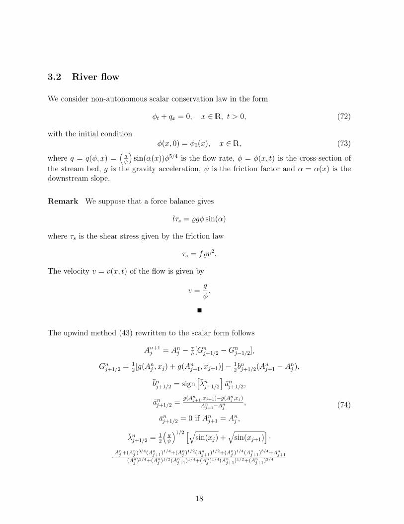
Figure 2: River flow: aL = 0.2, aR = 0.1, αL = π10

, αR = π20

, h = 0.01, τ = h/6, tmax = 0.33

3.3 Fluid flow through the male urethra I

In one space dimension the fluid flow through the male urethra is governed by the followingsystem of equations

φt + (vφ)x = 0, x ∈ (0, L), t ∈ (0, T ),vt + (1

2v2)x + 1

%px = 0, x ∈ (0, L), t ∈ (0, T ),

p = φ−ψ(x)β(x)

,(75)

where we denote the cross-section of the urethra by a = a(x, t), the fluid velocity byv = v(x, t), the fluid pressure by p = p(x, t). The fluid density is denoted by % and thematerial parameters (generally dependent on the space variable x) by ψ = ψ(x), β = β(x).This system can be written as the non-autonomous non-linear system in the form

qt + [g(q, x)]x = 0,

q = [φ, v]T , g =[vφ, 1

2v2 + φ−ψ(x)

β(x)%

]T,

(76)

or as the autonomous non-linear system in the form

ut + [f(u)]x = 0,

u = [φ, v, w]T , f =[vφ, 1

2v2 + φ−ψ(w)

β(w)%, 0

]T.

(77)

This system has to be supplemented by the initial condition

w(x, 0) = x, x ∈ (0, L). (78)

19

The Jacobi matrix has the form

A(u) = fu =

v φ 01

β(w)%v −β(w)ψw+[ψ(w)−φ]βw

%β2(w)

0 0 0

. (79)

The eigenvalues of this system are

λ1 = v +√

φβ(x)%

,

λ2 = v −√

φβ(x)%

,

λ3 = 0.

(80)

The matrix (A11)nj+1/2 has the form

(A11)nj+1/2 =

[V n

j+1/2 Φnj+1/2

Kj+1/2 V nj+1/2

](81)

[(A11)

nj+1/2

]−1=

−V nj+1/2

Φnj+1/2

Knj+1/2

−(V nj+1/2

)2

Φnj+1/2

Φnj+1/2

Knj+1/2

−(V nj+1/2

)2

Kj+1/2

Φnj+1/2

Knj+1/2

−(V nj+1/2

)2

−V nj+1/2

Φnj+1/2

Knj+1/2

−(V nj+1/2

)2

(82)

whereΦn

j+1/2 = 12

(Φn

j + Φnj+1

),

V nj+1/2 = 1

2

(V n

j + V nj+1

),

Kj+1/2 = 12

(1

%βj+ 1

%βj+1

).

(83)

The eigenvalues are

λn,1j+1/2 = V n

j+1/2 +√

Φnj+1/2Kj+1/2,

λn,2j+1/2 = V n

j+1/2 −√

Φnj+1/2Kj+1/2.

(84)

The matrix of the right eigenvectors is

(S11)nj+1/2 =

√Φn

j+1/2

Kj+1/2−

√Φn

j+1/2

Kj+1/2

1 1

=

[(s11)

n,1j+1/2, (s11)

n,2j+1/2

], (85)

and the inverse matrix has the form

[(S11)

nj+1/2

]−1=

12

√Kj+1/2

Φnj+1/2

12

−12

√Kj+1/2

Φnj+1/2

12

. (86)

Anj+1/2 =

V nj+1/2 Φn

j+1/2 0

Kj+1/2 V nj+1/2

Φnj+1/2

Kj+1/2+Lnj+1/2

h

0 0 0

(87)

20

where

Lnj+1/2 =

Ψnj

%βj

− Ψnj+1

%βj+1

, Knj+1/2 =

1

%βj+1

− 1

%βj

. (88)

Snj+1/2 =

√Φn

j+1/2

Knj+1/2

−√

Φnj+1/2

Knj+1/2

Mnj+1/2

1 1 Nnj+1/2

0 0 1

(89)

[Sn

j+1/2

]−1=

12

√Kn

j+1/2

Φnj+1/2

12−1

2Nn

j+1/2 − 12Mn

j+1/2

√Kn

j+1/2

Φnj+1/2

−12

√Kn

j+1/2

Φnj+1/2

12−1

2Nn

j+1/2 + 12Mn

j+1/2

√Kn

j+1/2

Φnj+1/2

0 0 1

(90)

Mnj+1/2 =

−Φnj+1/2

(Φn

j+1/2Kn

j+1/2+Ln

j+1/2

)

h

[Φn

j+1/2Kn

j+1/2−(V n

j+1/2)2]

Nnj+1/2 =

V nj+1/2

(Φn

j+1/2Kn

j+1/2+Ln

j+1/2

)

h

[Φn

j+1/2Kn

j+1/2−(V n

j+1/2)2]

(91)

References

[BLMR02] D. S. Bale, R. J. LeVeque, S. Mitran, and J. A. Rossmanith. A wave propaga-tion method for conservation laws and balance laws with spatially varying fluxfunctions. SIAM J. Sci. Comput., Accepted 2002.

[BM02] M. Brandner and S. Mıka. Numerical methods for conservation laws. In Pro-gramy a algoritmy numericke matematiky, volume 11. Mathematical Instituteof Czech Academy of Sciences, 2002.

[HL96] B. T. Hayes and P. G. LeFloch. Nonclassical shock waves and kinetic relations(II). Technical report, CMAP, Ecole Polytechnique (France), 1996.

[HL97] B. Hayes and P. G. LeFloch. Nonclassical shocks and kinetic relations: Scalarconservation laws. Arch. Rational Mech. Anal., 139:1–56, 1997.

[JT98] G. S. Jiang and E. Tadmor. Nonoscillatory central schemes for multidimen-sional hyperbolic conservation laws. SIAM J. Sci. Comput., 19(6), 1998.

[KR99] C. Klingenberg and N. H. Risebro. Stability of a resonant system of conserva-tion laws modeling polymer flow with gravitation. Conservation Laws Serverhttp://www.math.ntnu.no/conservation/, 1999.

21

0 0.1 0.2 0.3 0.4 0.50

0.5

1

1.5x 10

−3

cross−area

0 0.1 0.2 0.3 0.4 0.50

5

10

15

velocity

0 0.1 0.2 0.3 0.4 0.50

1

2x 10

5

pressure

0 0.1 0.2 0.3 0.4 0.5−4

−2

0x 10

−4

ψ

0 0.1 0.2 0.3 0.4 0.52

4

6

8x 10

−9

β

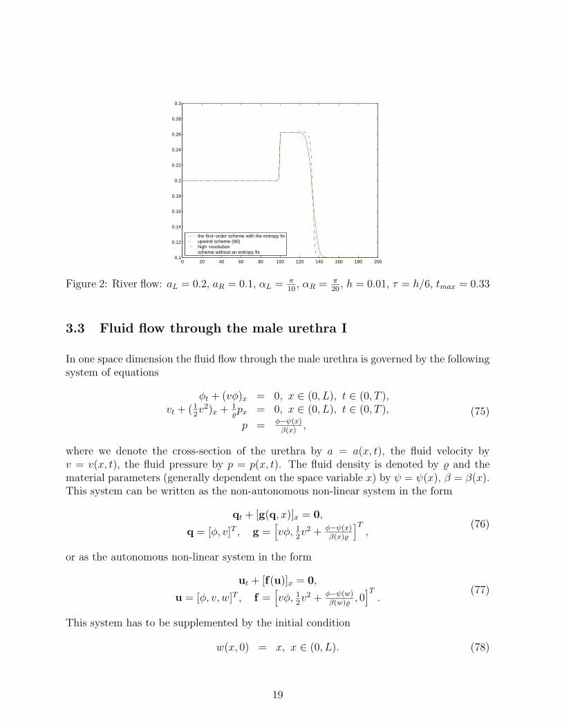
Figure 3: Fluid flow through the (simplified) mail urethra: h = 0.01, τ = h/2, tmax = 0.75

22

[LeV01] R. J. LeVeque. Finite volume methods for nonlinear elasticity in heterogeneousmedia. In Proceedings of the ICFD Conference. Oxford University, 2001.

[LL00] J. O. Langseth and R. J. LeVeque. A wave propagation method for three-dimensional hyperbolic conservation laws. Journal of Computational Physics,165(1):126–166, 2000.

[LTJ95] L. Longwei, B. Temple, and W. Jinghua. Suppression of oscillations in go-dunov’s method for a resonant non-strictly hyperbolic system. SIAM J. Numer.Anal., 32(3):841–864, 1995.

[LTW95] L. Lin, J. B. Temple, and J. Wang. A comparison of convergence rates forgodunov’s and glimm’s method in resonant nonlinear systems of conservationlaws. SIAM J. Numer. Anal., 32(3):824–840, 1995.

[MS98] L. Margolin and P. K. Smolarkiewicz. Antidiffusive velocities for multipassdonor cell advection. SIAM J. Sci. Comput., 20(3), 1998.

[SM98] P. K. Smolarkiewicz and L. G. Margolin. MPDATA: A finite-difference solverfor geophysical flows. Journal of Computational Physics, 140:459–480, 1998.

[Sur00] A. Suresh. Positivity-preserving schemes in multidimensions. SIAM J. Sci.Comput., 22(4), 2000.

[Tow00] J. D. Towers. Convergence of a difference scheme for conservation laws with adiscontinuous flux. SIAM J. Numer. Anal., 38(2), 2000.

[Tow01] J. D. Towers. A difference scheme for conservation laws with a discontinuousflux: The nonconvex case. SIAM J. Numer. Anal., 39(4), 2001.

23