lable at ScienceDirect

Environmental Pollution 185 (2014) 44e51

Contents lists avai

Environmental Pollution

journal homepage: www.elsevier .com/locate/envpol

Spatially-varying surface roughness and ground-level air quality in anoperational dispersion modelq

M.J. Barnes a, T.K. Brade a, A.R. MacKenzie b,*, J.D. Whyatt a, D.J. Carruthers c, J. Stocker c,X. Cai b, C.N. Hewitt a

a Lancaster Environment Centre, Lancaster University, LA1 4YW, UKb School of Geography, Earth and Environmental Sciences, University of Birmingham, B15 2TT, UKcCambridge Environmental Research Consultants Ltd, 3 Kings Parade, Cambridge CB2 1SJ, UK

a r t i c l e i n f o

Article history:Received 24 May 2013Received in revised form23 August 2013Accepted 20 September 2013

Keywords:Air qualityADMS-UrbanAerodynamic roughnessStreet canyonsUrban breathability

q This is an open-access article distributed undeCommons Attribution License, which permits unresreproduction in any medium, provided the original au* Corresponding author.

E-mail address: a.r.mackenzie@bham.ac.uk (A.R. M

0269-7491/$ e see front matter � 2013 The Authors.http://dx.doi.org/10.1016/j.envpol.2013.09.039

a b s t r a c t

Urban form controls the overall aerodynamic roughness of a city, and hence plays a significant role inhow air flow interacts with the urban landscape. This paper reports improved model performanceresulting from the introduction of variable surface roughness in the operational air-quality model ADMS-Urban (v3.1). We then assess to what extent pollutant concentrations can be reduced solely through localreductions in roughness. The model results suggest that reducing surface roughness in a city centre canincrease ground-level pollutant concentrations, both locally in the area of reduced roughness anddownwind of that area. The unexpected simulation of increased ground-level pollutant concentrationsimplies that this type of modelling should be used with caution for urban planning and design studieslooking at ventilation of pollution. We expect the results from this study to be relevant for all atmo-spheric dispersion models with urban-surface parameterisations based on roughness.

� 2013 The Authors. Published by Elsevier Ltd. All rights reserved.

1. Introduction

It has been estimated that over 1 billion people are exposed topoor air quality, and that it causes 1 million premature deaths eachyear (World Health Organization, 2005; United Nations, 2010). Inprinciple, there are four ways to reduce exposure to poor urban airquality and improve the health of the inhabitants of a city: reduceoverall emissions (Mayer, 1999); increase the depositional sink forpollutants (Nowak et al., 2000); relocate people and/or pollutingindustries (i.e., better segregation between pollutant sources andvulnerable populations) (Okuda et al., 2011); or improve theventilation of city neighbourhoods and streets (Vardoulakis et al.,2011).

The ventilation of a city is intricately linked with urban formbecause urban form (i) controls the overall aerodynamic roughnessof the urban area, (ii) produces specific quasi-stationary modifica-tions to the impinging flow (e.g., venturi effects, cross-wind flows,wakes, vortices, etc), and (iii) interacts with the radiative and

r the terms of the Creativetricted use, distribution, andthor and source are credited.

acKenzie).

Published by Elsevier Ltd. All righ

turbulent energy transfer between surface and atmosphere, andeffects heat storage in the underlying surface or buildings. Surfaceaerodynamic roughness is a function of the spatial density, orien-tation and height of obstacles to the wind and plays a significantrole in how air flow interacts with the urban landscape (Mahrt,1999; Holland et al., 2008; Di Sabatino et al., 2010; Salizzoniet al., 2011). Historically, few users had the computational powerto model spatially varying roughness, hence single (fixed) valueswere adopted (Rotach,1993; Kastner-Klein et al., 2004). However, itis now possible to account for the effects of variable surfaceroughness using models that run on desktop computers(Edussuriya et al., 2011; Millward-Hopkins et al., 2011; Soulhacet al., 2011).

In classical, one-dimensional, boundary-layer theory, surfaceroughness is parameterized through the roughness length (z0),which is equivalent to the height where the mean wind speedbecomes zero (Seinfeld and Pandis, 2006; Holland et al., 2008; Liet al., 2009). is approximately one thirtieth of the height of thesurface roughness elements, with values ranging from 1.5 m forlarge urban areas, to 0.5 m for open suburbia and 0.1 m for parkland(Rotach, 2001; Hang and Li, 2011; Wania et al., 2012). Roughnesslength varies greatly from the dense, compact and often high-risedcity centres to the more homogeneous areas found on the outskirts,especially those of older European cities (Grimmond and Oke,1999;Roth, 2000; Ng et al., 2011). Spatially-variable roughness creates

ts reserved.

M.J. Barnes et al. / Environmental Pollution 185 (2014) 44e51 45

horizontal variations in turbulence and the local mean flow, both ofwhich can affect pollutant dispersion.

Overall, the degree to which an urban form promotes theremoval and dilution of pollutants is encapsulated in the concept of‘urban breathability’ (Bottema, 1997; Monks et al., 2009; Buccolieriet al., 2010; Panagiotou et al., 2013), which is defined by Neophytouet al. (2005) and Buccolieri et al. (2011) as a parameter indicatingthe potential of a city to ventilate itself through the exchange ofpollutants, heat, moisture and other scalars with the atmosphereabove. Operational dispersion modelling does not explicitly simu-late the urban canopy and its exchange with the planetaryboundary layer above, but attempts to capture ”breathability”through canyon parameterisations and aerodynamic roughness.

ADMS-Urban is a tool for modelling air quality at a city-widescale, and can include industrial, domestic and traffic emissions.Many recent studies have verified the accuracy of the model(Courthold and Whitwell, 1998; Righi et al., 2009; Mohan et al.,2011), while others have used it to assess the effects of climatechange on air quality (Athanassiadou et al., 2010) or to estimatebackground urban carbon monoxide concentrations (Leuzzi et al.,2010). Additionally, many local authorities use ADMS-Urban toevaluate changes in air quality associated with major infra-structural developments, or to assess the potential impact of trafficmanagement schemes (Oduyemi and Davidson, 1998), or changesin fleet composition (Rexeis and Hausberger, 2009).

The current version of ADMS-Urban allows users to model thespatial variation of surface roughness over a given modellingdomain. In previous versions of the model, users were restricted tospecifying a single roughness value for the entire urban area, or elsemodelling the spatial variation of terrain height together with thesurface roughness. ADMS-Urban is proprietorial model code,although details of the algorithms are available via the companywebsite and are based on research published in various journalarticles (Carruthers et al., 2001). It is a steady-state quasi-Gaussianplume model, which contains the FLOWSTAR model (Belcher andHunt, 1998) for calculating the spatial variation of flow field andturbulence parameters that drive the dispersion. FLOWSTAR cal-culates the perturbations to the mean wind speed boundary layerprofile, u, which is formulated as:

uðzÞ ¼ u�k

�ln�zþ z0z0

�þ jðz; z0; LÞ

�(1)

This formulation illustrates that the mean wind speed at heightz is a function of surface roughness z0, stability through the functionj, and the friction velocity u* (k is the von Kármán constant and L isthe Monin-Obukhov length).

It is useful to note at this point that the expression for the meanwind speed used in ADMS-Urban (1) does not allow for thedisplacement of the wind speed profile to above the urban canopy.Instead, the local value of z0 represents the mixing close to thesurface, and is related to the building height. An alternativeformulation, that includes this zero-plane displacement height, d, isgiven by:

uðzÞ ¼ u�k

�ln�z� dz0

�þ jðz; z0; L;dÞ

�(2)

This paper has two aims.

� To assess changes in model performance resulting from theimplementation of variable roughness values in ADMS-Urban,and

� To use the best model representation to assess the air-qualitybenefits of improving ventilation.

Based on the literature discussed above, our hypothesis is thatselectively decreasing surface roughness for part of the built-upurban area will improve ventilation and hence reduce localpollutant concentrations. To examine our hypothesis, we mustundertake the first evaluation of the effect of spatially-varyingroughness in ADMS-Urban. To aid interpretation of the modelling,we will work in the framework of the Gaussian Plume Equation(GPE, see Seinfeld and Pandis (2006) ch. 18), a commonly usedversion of which is:

Cðx; y; zÞ ¼ q2psysz

�u� exp

� y2

2s2y

!"exp

� ðh� zÞ2

2s2z

!

þ exp

� ðhþ zÞ2

2s2z

!# (3)

where C is the concentration at point (x,y,z) (kg m�3) which isdirectly proportional to q, the mass emission rate (g s�1) (Turner,1994). sy is the standard deviation of Gaussian distribution func-tion in direction y (m), sz is the standard deviation of Gaussiandistribution function in direction z (m), hui is the wind speed(m s�1) averaged over the vertical and horizontal domain of thedispersion model, and h is the effective plume release height (m),which for road vehicles is taken as 1 m in ADMS-Urban. The s

parameters depend principally on the travel time of the pollutantfrom the source and the relevant components of the turbulentvelocities, which near the ground depend principally on the surfacefriction velocity, which in turn is a function of surface roughness.The domain-average wind, hui, depends on the geostrophic windand surface roughness. Both the plume spread and mean windspeed depend on stability effects.

The effect of changing roughness on ground-level pollutantconcentrations near a ground-level sourcewill therefore depend onthe relative sensitivities to z0 of sz and sy on the one hand (see theappendix), and of hui, sensitivities whichwill tend to have opposingeffects on pollutant concentrations at a given point. This is dis-cussed further below where we refer to the opposing effects asbeing the turbulent mixing (i.e., the sz and sy) sensitivity and thehorizontal ventilation (the hui sensitivity).

2. Model set-up, evaluation, and effects of variable roughness

As our test case, we use a modelling scenario for central Bir-mingham, UK. The model area of interest covered 6.5 km2 of Bir-mingham city centre (UK grid reference for the bottom-left cornere406274, 285376), containing over 300 road sources (Fig. 1). ADMS-Urban allows for the effects of street canyons when modellingpollutant concentrations, and many of the roads in the area of in-terest were classified as canyons with heights varying from 5 to20m. The 2008 emission inventory built into ADMS-Urbanwas usedto model traffic emissions, while background pollutant concentra-tions were obtained from the UK government’s Automatic Urbanand Rural Network (AURN) of air quality monitors, where onemonitor is situatedwithin the city centre (www.uk-air.defra.gov.uk).Annual mean backgrounds of 34.8 mg m�3 and 23.1 mg m�3 wereadopted forNOx andNO2, respectively. One year of hourly sequentialmeteorological data from Coleshill Met station (inset, Fig. 1) wasused in the model runs. We follow standard practice in choosing ameteorological station close to, but not inside the urban area of in-terest (Oke, 2006). This is because meteorological data fromwithinanurban area havewell-knownproblemsof representativeness. TheADMS-Urban modelling suite, used in this study, includes a mete-orological pre-processor that accounts for the change in roughnessassociated with moving from rural to urban land cover.

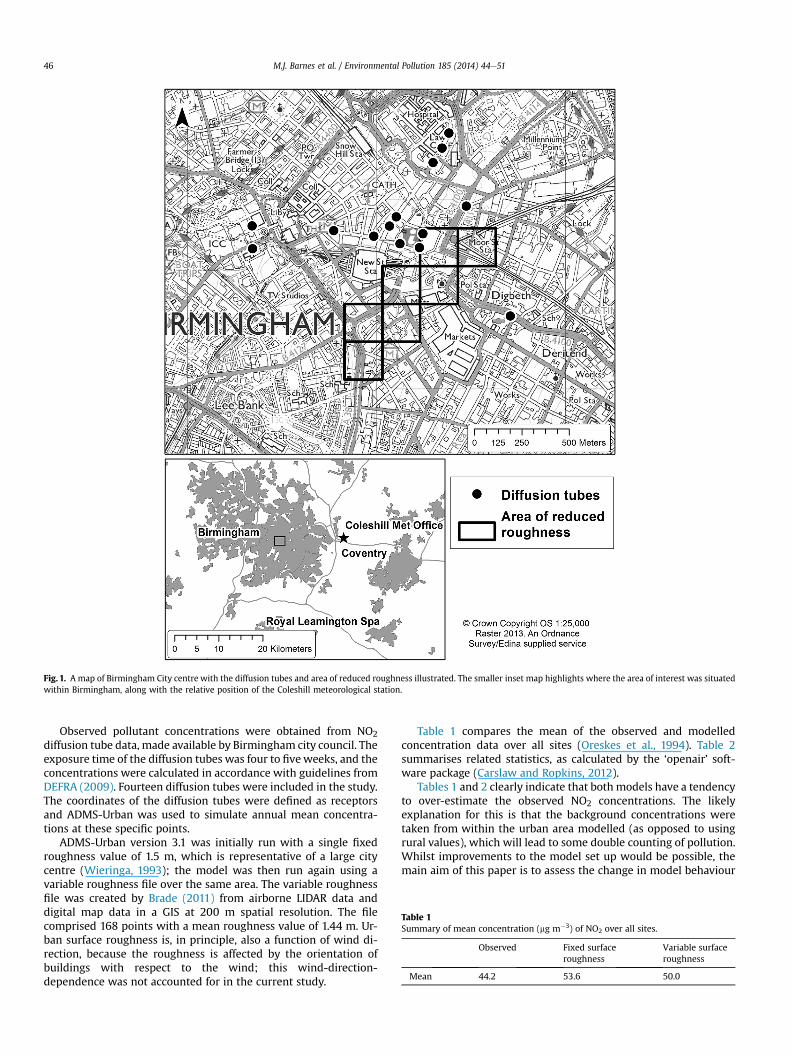
Fig. 1. A map of Birmingham City centre with the diffusion tubes and area of reduced roughness illustrated. The smaller inset map highlights where the area of interest was situatedwithin Birmingham, along with the relative position of the Coleshill meteorological station.

Table 1Summary of mean concentration (mg m�3) of NO2 over all sites.

Observed Fixed surfaceroughness

Variable surfaceroughness

Mean 44.2 53.6 50.0

M.J. Barnes et al. / Environmental Pollution 185 (2014) 44e5146

Observed pollutant concentrations were obtained from NO2diffusion tube data, made available by Birmingham city council. Theexposure time of the diffusion tubes was four to fiveweeks, and theconcentrations were calculated in accordance with guidelines fromDEFRA (2009). Fourteen diffusion tubes were included in the study.The coordinates of the diffusion tubes were defined as receptorsand ADMS-Urban was used to simulate annual mean concentra-tions at these specific points.

ADMS-Urban version 3.1 was initially run with a single fixedroughness value of 1.5 m, which is representative of a large citycentre (Wieringa, 1993); the model was then run again using avariable roughness file over the same area. The variable roughnessfile was created by Brade (2011) from airborne LIDAR data anddigital map data in a GIS at 200 m spatial resolution. The filecomprised 168 points with a mean roughness value of 1.44 m. Ur-ban surface roughness is, in principle, also a function of wind di-rection, because the roughness is affected by the orientation ofbuildings with respect to the wind; this wind-direction-dependence was not accounted for in the current study.

Table 1 compares the mean of the observed and modelledconcentration data over all sites (Oreskes et al., 1994). Table 2summarises related statistics, as calculated by the ‘openair’ soft-ware package (Carslaw and Ropkins, 2012).

Tables 1 and 2 clearly indicate that both models have a tendencyto over-estimate the observed NO2 concentrations. The likelyexplanation for this is that the background concentrations weretaken from within the urban area modelled (as opposed to usingrural values), which will lead to some double counting of pollution.Whilst improvements to the model set up would be possible, themain aim of this paper is to assess the change in model behaviour

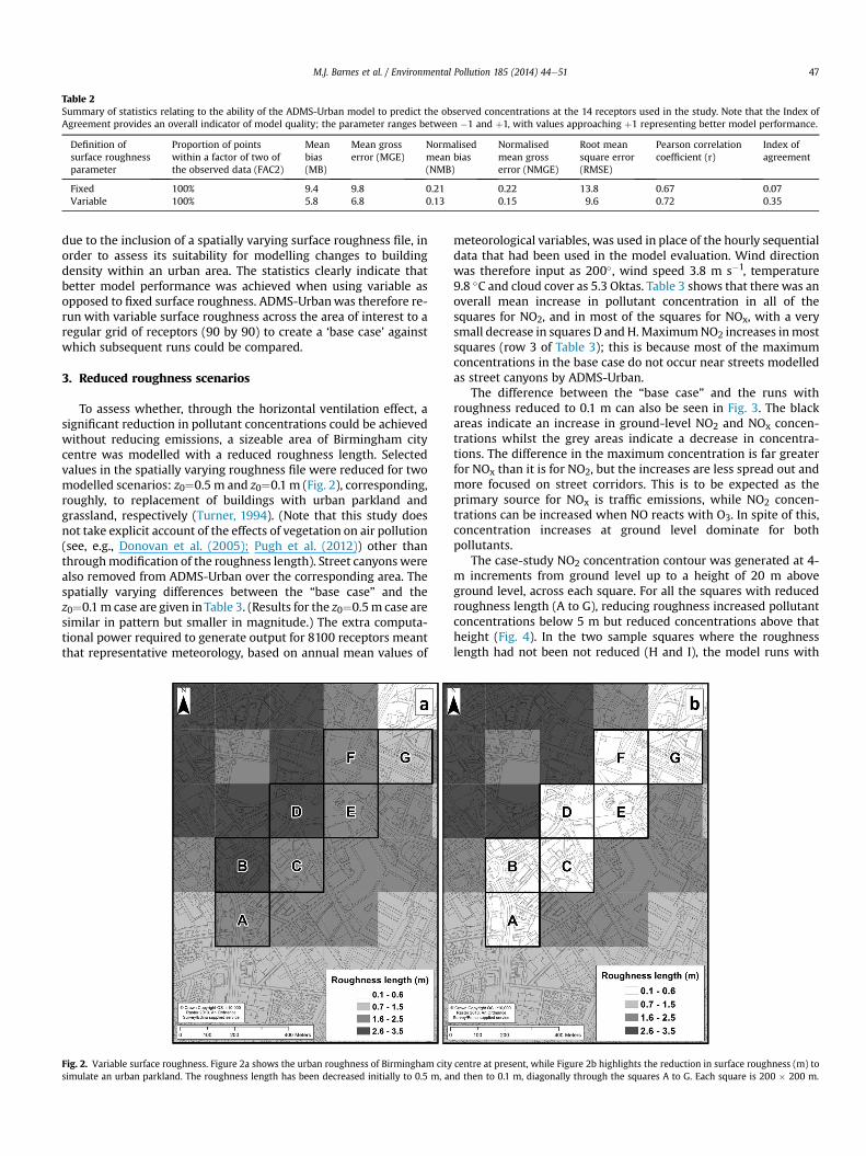
Table 2Summary of statistics relating to the ability of the ADMS-Urban model to predict the observed concentrations at the 14 receptors used in the study. Note that the Index ofAgreement provides an overall indicator of model quality; the parameter ranges between �1 and þ1, with values approaching þ1 representing better model performance.

Definition ofsurface roughnessparameter

Proportion of pointswithin a factor of two ofthe observed data (FAC2)

Meanbias(MB)

Mean grosserror (MGE)

Normalisedmean bias(NMB)

Normalisedmean grosserror (NMGE)

Root meansquare error(RMSE)

Pearson correlationcoefficient (r)

Index ofagreement

Fixed 100% 9.4 9.8 0.21 0.22 13.8 0.67 0.07Variable 100% 5.8 6.8 0.13 0.15 9.6 0.72 0.35

M.J. Barnes et al. / Environmental Pollution 185 (2014) 44e51 47

due to the inclusion of a spatially varying surface roughness file, inorder to assess its suitability for modelling changes to buildingdensity within an urban area. The statistics clearly indicate thatbetter model performance was achieved when using variable asopposed to fixed surface roughness. ADMS-Urbanwas therefore re-run with variable surface roughness across the area of interest to aregular grid of receptors (90 by 90) to create a ‘base case’ againstwhich subsequent runs could be compared.

3. Reduced roughness scenarios

To assess whether, through the horizontal ventilation effect, asignificant reduction in pollutant concentrations could be achievedwithout reducing emissions, a sizeable area of Birmingham citycentre was modelled with a reduced roughness length. Selectedvalues in the spatially varying roughness file were reduced for twomodelled scenarios: z0¼0.5 m and z0¼0.1 m (Fig. 2), corresponding,roughly, to replacement of buildings with urban parkland andgrassland, respectively (Turner, 1994). (Note that this study doesnot take explicit account of the effects of vegetation on air pollution(see, e.g., Donovan et al. (2005); Pugh et al. (2012)) other thanthroughmodification of the roughness length). Street canyonswerealso removed from ADMS-Urban over the corresponding area. Thespatially varying differences between the “base case” and thez0¼0.1m case are given in Table 3. (Results for the z0¼0.5m case aresimilar in pattern but smaller in magnitude.) The extra computa-tional power required to generate output for 8100 receptors meantthat representative meteorology, based on annual mean values of

Fig. 2. Variable surface roughness. Figure 2a shows the urban roughness of Birmingham citysimulate an urban parkland. The roughness length has been decreased initially to 0.5 m, an

meteorological variables, was used in place of the hourly sequentialdata that had been used in the model evaluation. Wind directionwas therefore input as 200�, wind speed 3.8 m s�1, temperature9.8 �C and cloud cover as 5.3 Oktas. Table 3 shows that there was anoverall mean increase in pollutant concentration in all of thesquares for NO2, and in most of the squares for NOx, with a verysmall decrease in squares D and H.MaximumNO2 increases inmostsquares (row 3 of Table 3); this is because most of the maximumconcentrations in the base case do not occur near streets modelledas street canyons by ADMS-Urban.

The difference between the “base case” and the runs withroughness reduced to 0.1 m can also be seen in Fig. 3. The blackareas indicate an increase in ground-level NO2 and NOx concen-trations whilst the grey areas indicate a decrease in concentra-tions. The difference in the maximum concentration is far greaterfor NOx than it is for NO2, but the increases are less spread out andmore focused on street corridors. This is to be expected as theprimary source for NOx is traffic emissions, while NO2 concen-trations can be increased when NO reacts with O3. In spite of this,concentration increases at ground level dominate for bothpollutants.

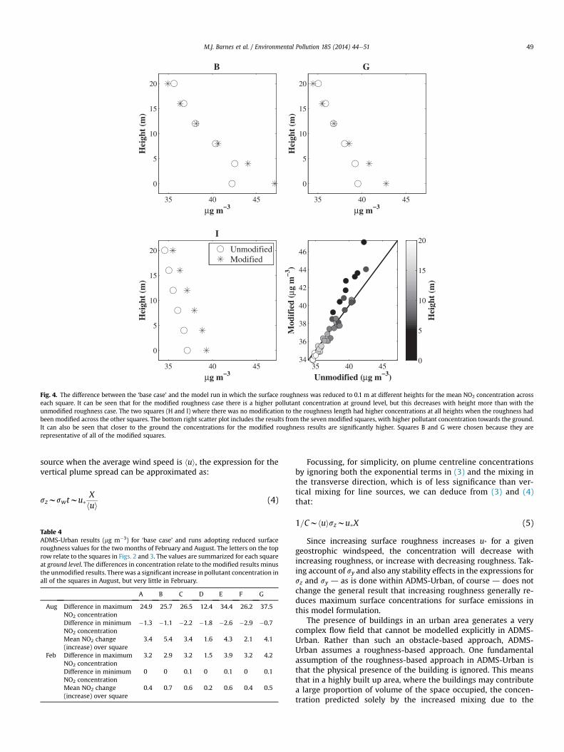
The case-study NO2 concentration contour was generated at 4-m increments from ground level up to a height of 20 m aboveground level, across each square. For all the squares with reducedroughness length (A to G), reducing roughness increased pollutantconcentrations below 5 m but reduced concentrations above thatheight (Fig. 4). In the two sample squares where the roughnesslength had not been not reduced (H and I), the model runs with

centre at present, while Figure 2b highlights the reduction in surface roughness (m) tod then to 0.1 m, diagonally through the squares A to G. Each square is 200 � 200 m.

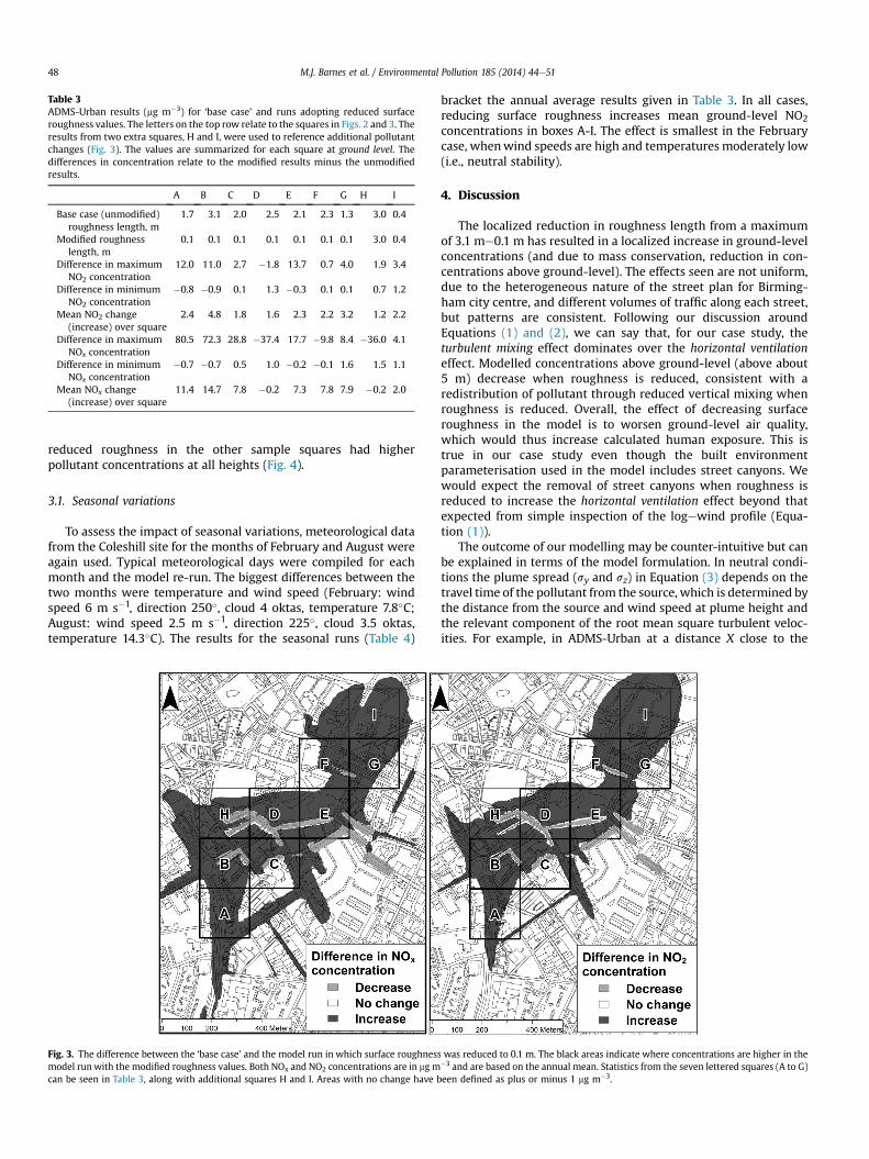
Table 3ADMS-Urban results (mg m�3) for ‘base case’ and runs adopting reduced surfaceroughness values. The letters on the top row relate to the squares in Figs. 2 and 3. Theresults from two extra squares, H and I, were used to reference additional pollutantchanges (Fig. 3). The values are summarized for each square at ground level. Thedifferences in concentration relate to the modified results minus the unmodifiedresults.

A B C D E F G H I

Base case (unmodified)roughness length, m

1.7 3.1 2.0 2.5 2.1 2.3 1.3 3.0 0.4

Modified roughnesslength, m

0.1 0.1 0.1 0.1 0.1 0.1 0.1 3.0 0.4

Difference in maximumNO2 concentration

12.0 11.0 2.7 �1.8 13.7 0.7 4.0 1.9 3.4

Difference in minimumNO2 concentration

�0.8 �0.9 0.1 1.3 �0.3 0.1 0.1 0.7 1.2

Mean NO2 change(increase) over square

2.4 4.8 1.8 1.6 2.3 2.2 3.2 1.2 2.2

Difference in maximumNOx concentration

80.5 72.3 28.8 �37.4 17.7 �9.8 8.4 �36.0 4.1

Difference in minimumNOx concentration

�0.7 �0.7 0.5 1.0 �0.2 �0.1 1.6 1.5 1.1

Mean NOx change(increase) over square

11.4 14.7 7.8 �0.2 7.3 7.8 7.9 �0.2 2.0

M.J. Barnes et al. / Environmental Pollution 185 (2014) 44e5148

reduced roughness in the other sample squares had higherpollutant concentrations at all heights (Fig. 4).

3.1. Seasonal variations

To assess the impact of seasonal variations, meteorological datafrom the Coleshill site for the months of February and August wereagain used. Typical meteorological days were compiled for eachmonth and the model re-run. The biggest differences between thetwo months were temperature and wind speed (February: windspeed 6 m s�1, direction 250�, cloud 4 oktas, temperature 7.8�C;August: wind speed 2.5 m s�1, direction 225�, cloud 3.5 oktas,temperature 14.3�C). The results for the seasonal runs (Table 4)

Fig. 3. The difference between the ‘base case’ and the model run in which surface roughnesmodel runwith the modified roughness values. Both NOx and NO2 concentrations are in mg mcan be seen in Table 3, along with additional squares H and I. Areas with no change have b

bracket the annual average results given in Table 3. In all cases,reducing surface roughness increases mean ground-level NO2concentrations in boxes A-I. The effect is smallest in the Februarycase, whenwind speeds are high and temperatures moderately low(i.e., neutral stability).

4. Discussion

The localized reduction in roughness length from a maximumof 3.1 me0.1 m has resulted in a localized increase in ground-levelconcentrations (and due to mass conservation, reduction in con-centrations above ground-level). The effects seen are not uniform,due to the heterogeneous nature of the street plan for Birming-ham city centre, and different volumes of traffic along each street,but patterns are consistent. Following our discussion aroundEquations (1) and (2), we can say that, for our case study, theturbulent mixing effect dominates over the horizontal ventilationeffect. Modelled concentrations above ground-level (above about5 m) decrease when roughness is reduced, consistent with aredistribution of pollutant through reduced vertical mixing whenroughness is reduced. Overall, the effect of decreasing surfaceroughness in the model is to worsen ground-level air quality,which would thus increase calculated human exposure. This istrue in our case study even though the built environmentparameterisation used in the model includes street canyons. Wewould expect the removal of street canyons when roughness isreduced to increase the horizontal ventilation effect beyond thatexpected from simple inspection of the logewind profile (Equa-tion (1)).

The outcome of our modelling may be counter-intuitive but canbe explained in terms of the model formulation. In neutral condi-tions the plume spread (sy and sz) in Equation (3) depends on thetravel time of the pollutant from the source, which is determined bythe distance from the source and wind speed at plume height andthe relevant component of the root mean square turbulent veloc-ities. For example, in ADMS-Urban at a distance X close to the

s was reduced to 0.1 m. The black areas indicate where concentrations are higher in the�3 and are based on the annual mean. Statistics from the seven lettered squares (A to G)een defined as plus or minus 1 mg m�3.

35 40 45

0

5

10

15

20

B

Hei

ght

(m)

µg m−335 40 45

0

5

10

15

20

G

Hei

ght

(m)

µg m−3

35 40 45

0

5

10

15

20

I

Hei

ght

(m)

µg m−3

UnmodifiedModified

35 40 4534

36

38

40

42

44

46

Unmodified (µg m−3)

Mod

ifie

d (µ

g m

−3)

Hei

ght

(m)

0

5

10

15

20

Fig. 4. The difference between the ‘base case’ and the model run in which the surface roughness was reduced to 0.1 m at different heights for the mean NO2 concentration acrosseach square. It can be seen that for the modified roughness case there is a higher pollutant concentration at ground level, but this decreases with height more than with theunmodified roughness case. The two squares (H and I) where there was no modification to the roughness length had higher concentrations at all heights when the roughness hadbeen modified across the other squares. The bottom right scatter plot includes the results from the seven modified squares, with higher pollutant concentration towards the ground.It can also be seen that closer to the ground the concentrations for the modified roughness results are significantly higher. Squares B and G were chosen because they arerepresentative of all of the modified squares.

M.J. Barnes et al. / Environmental Pollution 185 (2014) 44e51 49

source when the average wind speed is hui, the expression for thevertical plume spread can be approximated as:

szwswtwu�Xhui (4)

Table 4ADMS-Urban results (mg m�3) for ‘base case’ and runs adopting reduced surfaceroughness values for the two months of February and August. The letters on the toprow relate to the squares in Figs. 2 and 3. The values are summarized for each squareat ground level. The differences in concentration relate to the modified results minusthe unmodified results. Therewas a significant increase in pollutant concentration inall of the squares in August, but very little in February.

A B C D E F G

Aug Difference in maximumNO2 concentration

24.9 25.7 26.5 12.4 34.4 26.2 37.5

Difference in minimumNO2 concentration

�1.3 �1.1 �2.2 �1.8 �2.6 �2.9 �0.7

Mean NO2 change(increase) over square

3.4 5.4 3.4 1.6 4.3 2.1 4.1

Feb Difference in maximumNO2 concentration

3.2 2.9 3.2 1.5 3.9 3.2 4.2

Difference in minimumNO2 concentration

0 0 0.1 0 0.1 0 0.1

Mean NO2 change(increase) over square

0.4 0.7 0.6 0.2 0.6 0.4 0.5

Focussing, for simplicity, on plume centreline concentrationsby ignoring both the exponential terms in (3) and the mixing inthe transverse direction, which is of less significance than ver-tical mixing for line sources, we can deduce from (3) and (4)that:

1=Cwhuiszwu�X (5)

Since increasing surface roughness increases u* for a givengeostrophic windspeed, the concentration will decrease withincreasing roughness, or increase with decreasing roughness. Tak-ing account of sy and also any stability effects in the expressions forsz and sy d as is done within ADMS-Urban, of course d does notchange the general result that increasing roughness generally re-duces maximum surface concentrations for surface emissions inthis model formulation.

The presence of buildings in an urban area generates a verycomplex flow field that cannot be modelled explicitly in ADMS-Urban. Rather than such an obstacle-based approach, ADMS-Urban assumes a roughness-based approach. One fundamentalassumption of the roughness-based approach in ADMS-Urban isthat the physical presence of the building is ignored. This meansthat in a highly built up area, where the buildings may contributea large proportion of volume of the space occupied, the concen-tration predicted solely by the increased mixing due to the

Table A.1Value of zcrit/sz for different conditions.

sz ¼ 1 m sz ¼ 2 m sz ¼ 3 m sz ¼ 4 m

h ¼ 0.5 m 1.17 1.10 1.07 1.05h ¼ 1.0 m 1.92 1.42 1.27 1.20

M.J. Barnes et al. / Environmental Pollution 185 (2014) 44e5150

presence of buildings would lead to an underestimate of thepredicted concentrations. In order to account for this, ADMS-Urban includes a relatively simple treatment of street canyons,based on the Operational Street Pollution Model (OSPM), in whichthe build-up of pollutants between buildings is taken into accountin particular parts of the domain. Note, however, that this increasein concentrations within the canyon is not accounted for outside thecanyon and that only a relatively small fraction of the urbanlandscape can be treated in this way in the model (see, forexample, the areas of ‘street canyon’ shown by decreases in airpollutant concentrations in Fig. 3). Another aspect of the problemis that there is no allowance for the vertical displacement of thewind profile in the model (see Equation (3)), and the lowerwindspeeds and turbulence levels between the buildings, as seenfor example, in wind tunnels (Di Sabatino et al., 2008; Carrutherset al., 2011). This effect would be diminished in the ventilationcorridor.

Sections of the city downwind of the area of change were alsoadversely affected (Squares H and I, Fig. 3). The model outcomesuggests that, when implementing an urban ventilation corridor,there needs to be an “exit” for air pollution, otherwise there willbe significant increases in pollution concentrations d and henceexposure d in built-up areas just downwind. Overall, however,the simplifications inherent in a roughness-based approach d

and the additional simplificiations inherent in the locally one-dimensional closure of a roughness-based surface scheme d

should make us sceptical of the realism of any of the model resultspresented here.

5. Conclusions

Implementation of an option to model variable roughnesswithin the air pollution dispersion model ADMS-Urban hasimproved model performance, although this does have the penaltyof a significant increase in run time. We have used the newvariable-roughness facility in ADMS-Urban to examine reducedroughness scenarios (without reducing emissions). Our case-studymodel produces increased ground-level pollutant concentrationsfor reduced surface roughness, both locally in the area of reducedroughness and downwind of that area. We discuss this modellingoutcome from the perspective of Gaussian dispersion, and intro-duce a turbulent mixing effect and a horizontal ventilation effect,whose sensitivities to changing roughness are such that they act inopposite ways on ground-level pollutant concentrations. In ourcase study, the turbulent mixing effect dominates. Since the modelpredicts that reducing roughness has the (at first glance) perverseeffect of increasing ground-level pollutant concentrations, wecaution against using this type of modelling for urban planningand design studies in which the concept of breathability isimportant.

We expect the results from this study to be relevant for all at-mospheric dispersion models with urban-surface parameter-isations based on 1-D roughness-based closure schemes. To theextent that such models reflect actual atmospheric behaviour, theresults presented are most relevant to those post-industrial“shrinking” cities (e.g., Kabisch (2007)) in which plots of landnext to transport corridors become vacant and derelict. However,there are well-known limitations of 1-D roughness-based closureschemes near the surface of urban areas (e.g., Oke (2006)). We hopethat the model case study reported here illustrates the cautionwithwhich modelling based on 1-D roughness-based closure should beviewed when undertaking urban redevelopment, and that ourmodelling will stimulate discussion and CFD analyses to investigatefurther this type of behaviour with a view to improving the per-formance of air-quality dispersion models.

Acknowledgements

We thank Birmingham City Council for provision of diffusiontube data. This work was carried out as part of the UK EPSRC Sus-tainable Urban Environment programme, grant no. EP/F007426/1.

Appendices

A. Appendix

For Equation (3), and with szfz0, we may examine the effects ofsmall perturbations in a parameter value, say, hui, or z0 (effectivelysz) by using the partial differential of C with respect to theparameter. For example, a small change in mean wind speed huiwill cause a change in C:

DC���hui

¼ dCdhuiD

u

¼�� Dhui

hui�C: (6)

That is, the relative change in hui reduces (due to theminus sign)the pollutant concentration by the same relative amount, which isthewell-knowndependence of pollutant dispersion onwind speed.We can derive a similar relationship for sz, which is slightly morecomplicated:

DC���sz

¼ dCdsz

Dsz ¼ Dszsz

C

2664�z�hsz

�2e�

ðz�hÞ22sz þ

�zþhsz

�2e�

ðzþhÞ22sz

e�ðz�hÞ22sz þ e�

ðzþhÞ22sz

� 1

3775

¼ Dszsz

C$½A� 1�(7)

If the first term in the square bracket is ignored, the relationshipwould be the same as that for wind speed. By letting A ¼ 1, we canfind the critical height zcrit, below which A < 1 and above whichA > 1. Therefore in the domainwhere z < zcrit, a small increase in szwill cause C to reduce, and a small decrease of sz will cause C toincrease. This is consistent with the modelling results in which adecrease of z0 (thus a decrease of sz because szfz0) caused C toincrease for small z (Fig. 4). Note that A is larger than 1 for z > zcritand a small decrease of sz will cause C to decrease in this part of thedomain.

Under the conditions given in themanuscript (h¼ 0.5m or 1m),several values of zcrit/sz are calculated and shown in Table A.1. Theresults show that zcrit is larger than sz.

References

Athanassiadou, M., Baker, J., Carruthers, D., Collins, W., Girnary, S., Hassell, D.,Hort, M., Johnson, C., Johnson, K., Jones, R., Thomson, D., Trought, N., Witham, C.,2010. An assessment of the impact of climate change on air quality at two UKsites. Atmos. Environ. 44, 1877e1886.

Belcher, S., Hunt, J., 1998. Turbulent flow over hills and waves. Annu. Rev. FluidMech. 30, 507e538.

Bottema, M., 1997. Urban roughness modelling in relation to pollutant dispersion.Atmos. Environ. 31, 3059e3075.

Brade, T., 2011. Urban Breathability: Exploring Urban Ventilation in Birminghamwith Geographic Information Systems. Master’s thesis. Lancaster University.

M.J. Barnes et al. / Environmental Pollution 185 (2014) 44e51 51

Buccolieri, R., Sandberg, M., Di Sabatino, S., 2010. City breathability and its link topollutant concentration distribution within urban-like geometries. Atmos. En-viron. 44, 1894e1903.

Buccolieri, R., Sandberg, M., Di Sabatino, S., 2011. An application of ventilation ef-ficiency concepts to the analysis of building density effects on urban flow andpollutant concentration. Int. J. Environ. Pollut. 47, 248e256.

Carruthers, D., Dickson, P., McHugh, C., Nixon, S., Oates, W., 2001. Determination ofcompliance with UK and EU air quality objectives from high-resolutionpollutant concentration maps calculated using ADMS-Urban. Int. J. Environ.Pollut. 16, 460e471, 6th International Conference on Harmonization withinAtmospherica Dispersion Modelling for Regulatory Purposes, Rouen, France, Oct11-14, 1999.

Carruthers, D.J., Seaton, M.D., McHugh, C.A., Sheng, X., Solazzo, E., Vanvyve, E., 2011.Comparison of the complex terrain algorithms incorporated into twocommonly used local-scale air pollution dispersion models (ADMS and AER-MOD) using a hybrid model. J. Air Waste Manag. Assoc. 61, 1227e1235. Air-and-Waste-Management-Association (AWMA) International Speciality Conferenceon Leapfrogging Opportunities for Air Quality Improvement, Xian, Peoples RChina, May 10-14, 2010.

Carslaw, D.C., Ropkins, K., 2012. Openair e an R package for air quality data analysis.Environ. Model. Softw. 27-28, 52e61.

Courthold, N., Whitwell, I., 1998. Testing the tools of air quality management: acomparison of predictions of nitrogen dioxide concentrations by the CALINE4and ADMS-Urban dispersion algorithms with monitored concentrations at theM4/M5 interchange in Bristol, UK. In: Brebbia, C.A., Ratto, C.F., Power, H. (Eds.),Air Pollution, vol. VI, pp. 859e868, 6th International Conference on Air Pollu-tion, Genoa, Italy, Sep. 29e30, 1998.

DEFRA, 2009. Local Air Quality Management Technical Guidance LAQM. TG(09).Di Sabatino, S., Buccolieri, R., Pulvirenti, B., Britter, R.E., 2008. Flow and pollutant

dispersion in street canyons using FLUENT and ADMS-Urban. Environ. Model.Assess. 13, 369e381.

Di Sabatino, S., Leo, L.S., Cataldo, R., Ratti, C., Britter, R.E., 2010. Construction ofdigital elevation models for a Southern European city and a comparativemorphological analysis with respect to Northern European and North Americancities. J. Appl. Meteorol. Climatol. 49, 1377e1396.

Donovan, R., Stewart, H., Owen, S., Mackenzie, A., Hewitt, C., 2005. Developmentand application of an urban tree air quality score for photochemical pollutionepisodes using the Birmingham, United Kingdom, area as a case study. Enrion.Sci. Technol. 39, 6730e6738.

Edussuriya, R., Chan, A., Ye, A., 2011. Urban morphology and air quality in denseresidential environments in Hong Kong. Part I: district-level analysis. Atmos.Environ. 45, 4789e4803.

Grimmond, C., Oke, T., 1999. Aerodynamic properties of urban areas derived, fromanalysis of surface form. J. Appl. Meteorol. 38, 1262e1292.

Hang, J., Li, Y., 2011. Age of air and air exchange efficiency in high-rise urban areasand its link to pollutant dilution. Atmos. Environ. 45, 5572e5585.

Holland, D.E., Berglund, J.A., Spruce, J.P., Mckellip, R.D., 2008. Derivation of effectiveaerodynamic surface roughness in urban areas from airborne Lidar terrain data.J. Appl. Meteorol. Climatol. 47, 2614e2626.

Kabisch, S., 2007. Urban shrinkage and challenges for the public health-care service.Gesundheitswesen 69, 514e520.

Kastner-Klein, P., Berkowicz, R., Britter, R., 2004. The influence of street architectureon flow and dispersion in street canyons. Meteorol. Atmos. Phys. 87, 121e131.

Leuzzi, G., Monti, P., Amicarelli, A., 2010. An urban scale model for pollutantdispersion in Rome. Int. J. Environ. Pollut. 40, 85e93, 10th International Con-ference on Harmonisation within Atmospheric Dispersion Modelling for Reg-ulatory Purposes, Sissi, Greece, Oct 17-20, 2005.

Li, L., Shaomin, L., Ziwei, X., Kun, Y., Xuhui, C., Li, J., Jiemin, W., 2009. The charac-teristics and parameterization of aerodynamic roughness length over hetero-geneous surfaces. Adv. Atmos. Sci. 26, 180e190.

Mahrt, L., 1999. Stratified atmospheric boundary layers. Boundary-layer Meteorol.90, 375e396. http://dx.doi.org/10.1023/A:1001765727956.

Mayer, H., 1999. Air pollution in cities. Atmos. Environ. 33, 4029e4037. Interna-tional Conference on Urban Climatology (ICUC 96), ESSEN, GERMANY, JUN 10,1996-JUN 14, 1997.

Millward-Hopkins, J.T., Tomlin, A.S., Ma, L., Ingham, D., Pourkashanian, M., 2011.Estimating aerodynamic parameters of urban-like surfaces with heterogeneousbuilding heights. Boundary-layer Meteorol. 141, 443e465.

Mohan, M., Bhati, S., Sreenivas, A., Marrapu, P., 2011. Performance evaluation ofAERMOD and ADMS-urban for Total Suspended Particulate Matter concentra-tions in Megacity Delhi. Aerosol Air Qual. Res. 11, 883e894.

Monks, P.S., Granier, C., Fuzzi, S., Stohl, A., Williams, M.L., Akimoto, H., Amann, M.,Baklanov, A., Baltensperger, U., Bey, I., Blake, N., Blake, R.S., Carslaw, K.,Cooper, O.R., Dentener, F., Fowler, D., Fragkou, E., Frost, G.J., Generoso, S.,Ginoux, P., Grewe, V., Guenther, A., Hansson, H.C., Henne, S., Hjorth, J.,Hofzumahaus, A., Huntrieser, H., Isaksen, I.S.A., Jenkin, M.E., Kaiser, J.,Kanakidou, M., Klimont, Z., 2009. Atmospheric composition change e globaland regional air quality. Atmos. Environ. 43, 5268e5350.

Neophytou, M., Goussis, D., Mastorakos, E., Britter, R., 2005. The conceptualdevelopment of a simple scale-adaptive reactive pollutant dispersion model.Atmos. Environ. 39, 2787e2794, 4th International Conference on Urban AirQuality, Prague, CZECH REPUBLIC, MAR 25-28, 2003.

Ng, E., Yuan, C., Chen, L., Ren, C., Fung, J.C.H., 2011. Improving the wind environmentin high-density cities by understanding urban morphology and surfaceroughness: a study in Hong Kong. Landscape Urban Plann. 101, 59e74.

Nowak, D., Civerolo, K., Rao, S., Sistla, G., Luley, C., Crane, D., 2000. A modeling studyof the impact of urban trees on ozone. Atmos. Environ. 34, 1601e1613.

Oduyemi, K., Davidson, B., 1998. The impacts of road traffic management on urbanair quality. Sci. Total Environ. 218, 59e66.

Oke, T., 2006. Instruments and Observing Methods Report No. 81. Initial Guidanceto Obtain Representative Meteorological Observations at Urban Sites. WorldMeteorological Organization.

Okuda, T., Matsuura, S., Yamaguchi, D., Umemura, T., Hanada, E., Orihara, H.,Tanaka, S., He, K., Ma, Y., Cheng, Y., Liang, L., 2011. The impact of the pollutioncontrol measures for the 2008 Beijing Olympic Games on the chemicalcomposition of aerosols. Atmos. Environ. 45, 2789e2794.

Oreskes, N., Shraderfrechette, K., Belitz, K., 1994. Verification, validation, andconfirmation of numerical-models in the Earth-Sciences. Science 263, 641e646.

Panagiotou, I., Neophytou, M.K.A., Hamlyn, D., Britter, R.E., 2013. City breathabilityas quantified by the exchange velocity and its spatial variation in real inho-mogeneous urban geometries: an example from central London urban area. Sci.Total Environ. 442, 466e477.

Pugh, T.A.M., MacKenzie, A.R., Whyatt, J.D., Hewitt, C.N., 2012. Effectiveness of greeninfrastructure for improvement of air quality in urban street canyons. Environ.Sci. Technol. 46, 7692e7699.

Rexeis, M., Hausberger, S., 2009. Trend of vehicle emission levels until 2020-Prog-nosis based on current vehicle measurements and future emission legislation.Atmos. Environ. 43, 4689e4698, 6th International Conference on Urban AirQuality, Nicosia, Cyprus, Mar 27-29, 2007.

Righi, S., Lucialli, P., Pollini, E., 2009. Statistical and diagnostic evaluation of theADMS-Urban model compared with an urban air quality monitoring network.Atmos. Environ. 43, 3850e3857.

Rotach, M., 1993. Turbulence close to a rough urban surface .1. Reynolds stress.Boundary-layer Meteorol. 65, 1e28.

Rotach, M., 2001. Simulation of urban-scale dispersion using a Lagrangian stochasticdispersion model. Boundary-layer Meteorol. 99, 379e410.

Roth, M., 2000. Review of atmospheric turbulence over cities. Q. J. R. Meteorol. Soc.126, 941e990.

Salizzoni, P., Marro, M., Soulhac, L., Grosjean, N., Perkins, R., 2011. Turbulent transferbetween street canyons and the overlying atmospheric boundary layer.Boundary-layer Meteorol. 141, 393e414. http://dx.doi.org/10.1007/s10546-011-9641-1.

Seinfeld, J., Pandis, S., 2006. Atmospheric Chemistry and Physics. John Wiley & Sons,Inc.

Soulhac, L., Salizzoni, P., Cierco, F.X., Perkins, R., 2011. The model sirane for atmo-spheric urban pollutant dispersion; part i, presentation of the model. Atmos.Environ. 45, 7379e7395.

Turner, D.B., 1994. Workbook of Atmospheric Dispersion Estimates: an Introductionto Dispersion Modeling. Lewis Publishers.

United Nations, 2010. State of the World’s Cities 2010/2011: Bridging the UrbanDivide. Earthscan.

Vardoulakis, S., Solazzo, E., Lumbreras, J., 2011. Intra-urban and street scale vari-ability of BTEX, NO2 and O-3 in Birmingham, UK: implications for exposureassessment. Atmos. Environ. 45, 5069e5078.

Wania, A., Bruse, M., Blond, N., Weber, C., 2012. Analysing the influence of differentstreet vegetation on traffic-induced particle dispersion using microscale sim-ulations. J. Environ. Manage. 94, 91e101.

Wieringa, J., 1993. Representative roughness parameters for homogeneous terrain.Boundary-layer Meteorol. 63, 323e363.

World Health Organization, 2005. WHO Air Quality Guidlines for Particulate Matter,Ozone, Nitrogen Dioxide and Sulfure Dioxide. Global Update 2005. SUmmary ofRisk Assessment. World Health Organization.