Fine-scale sedimentary structure: implications foracoustic remote sensing

K.B. Briggs a;�, K.L. Williams b, D.R. Jackson b, C.D. Jones b, A.N. Ivakin b;c,T.H. Orsi d

a Sea£oor Sciences Branch, Naval Research Laboratory, Stennis Space Center, MS 39529, USAb Applied Physics Laboratory, University of Washington, Seattle, WA 98105, USA

c Andreev Acoustics Institute, Shvernika 4, Moscow 117036, Russiad Planning Systems Incorporated, 115 Christian Lane, Slidell, LA 70458, USA

Received 23 December 1999; accepted 14 March 2001

Abstract

Detailed measurements of sediment properties and acoustic scattering were made at a carbonate sand^silt^claysite off Dry Tortugas in the Florida Keys. The sediment is characterized by varying scales of biologically controlledrandom roughness and heterogeneity as well as surficial stratification on centimeter scales. The interface roughnesswas determined from stereo photogrammetric digitization and parameterized by a power spectrum, whereas sedimentvolume heterogeneity was determined from core measurements and parameterized by first-order autoregressivemodels for sound speed and density fluctuations. In contrast to previous investigations, fine-scale sediment bulkdensity fluctuations were examined in sediment cores with computerized tomography in addition to the standardgravimetric technique. Furthermore, the strongly delineated sediment density and sound velocity transition layer wasparameterized by piecewise linear fits. These characterizations of the random and deterministic properties were used inacoustic scattering models in an effort to determine the feasibility of remotely measuring fine-scale features of theseafloor. The result was negative: older, low-resolution models gave moderately good fits to the acoustic data, but thefit did not improve for newer, higher-resolution models. It is suggested that scattering due to shell fragments must beincluded to account for all features observed in the scattering data at this site. Published by Elsevier Science B.V.

Keywords: sedimentation; bioturbation; acoustical properties; density; X-ray radiography

1. Introduction

Sound scattering by the sea £oor at high fre-quencies (10^100 kHz) is governed primarily bycentimeter-scale structure, including laminar strat-i¢cation, random heterogeneity and random

roughness. In discussing these scattering mecha-nisms, it is helpful to divide sediments into twoclasses: those that permit substantial penetrationof sound and those that do not. The former classtypically includes muds: low-bulk-density, ¢ne-grained, cohesive material with consequently littleimpedance contrast across the sediment^water in-terface. Because of this lack of impedance con-trast these sediments are more likely to scattersound from the sediment volume rather than

0025-3227 / 02 / $ ^ see front matter Published by Elsevier Science B.V.PII: S 0 0 2 5 - 3 2 2 7 ( 0 1 ) 0 0 2 3 2 - 8

* Corresponding author.Tel. : +1-206-543-1328; Fax: +1-206-543-6785.

E-mailaddress: kevin.briggs@nrlssc.navy.mil(K.B.Briggs).

MARGO 2993 23-4-02

Marine Geology 182 (2002) 141^159

www.elsevier.com/locate/margeo

from the interface. Coarser, sandy sediments, onthe other hand, have substantial impedance con-trast, and scattering originates primarily from therough sediment^water interface. These two con-trasting scattering mechanisms can be used as abasis for acoustic classi¢cation of sediments (Iva-kin, 1983, 1989, 1998c; Sternlicht, 1999), providedreasonably accurate scattering models are avail-able for interpreting the data. Models for the scat-tering of high-frequency sound by sediment vol-ume heterogeneities have been developed byseveral investigators (Ivakin and Lysanov, 1981;Ivakin, 1981, 1983, 1986; Hines, 1990; Pace,1994; Lyons et al., 1994; Yamamoto, 1996).Rough-interface scattering models have been pre-sented by Kuo (1964), Ivakin (1983), Jackson etal. (1986), and others.

Whereas progress has been made in under-standing volume and interface scattering throughcomparison of models and data, such compari-sons have employed simpli¢ed models, consideredonly a single scattering direction (backscattering),and su¡ered from insu⁄cient spatial resolutionin the accompanying environmental data (Ivakin,1981, 1983, 1989; Stanic et al., 1988, 1998;Jackson and Briggs, 1992; Briggs, 1994; D. Jack-son et al., 1996). Our goal is to use sedimentproperty data with measurement intervals equalto or less than the acoustic wavelength and bi-static scattering data (that is, data taken with dif-ferent incident and scattering directions) to testhow well recent models predict scattering. Thesenewer models treat the e¡ects of strati¢cation onscattering as well as the more general bistatic an-gular dependence. Following the usual practice,acoustic scattering by the sea £oor will be quan-ti¢ed in terms of the ‘scattering strength’ (Urick,1983) for both backscattering and bistatic scatter-ing.

Questions that arise in connection with high-frequency sound scattering by sediments are: (1)Which is the dominant cause of scattering, inter-face roughness or volume heterogeneity? (2) Does¢ne-scale sediment structure a¡ect scatteringstrength? and, conversely, (3) Can acoustic re-mote sensing of the sea £oor be used to determine¢ne-scale sediment structure? We will addressthese and other questions in the context of a

data set acquired at a site where the sedimentshared characteristics of the ¢ne-grained, low-den-sity type associated with dominant volume scat-tering and the high-impedance type associatedwith dominant roughness scattering.

Sediment heterogeneity can be characterized bysystematic measurements of sound velocity anddensity from sediment cores. The mean propertiescan be expressed in terms of vertical pro¢les ofgeoacoustic parameters (sediment density, com-pressional wave velocity, and absorption) andthe £uctuations about the mean can be parame-terized in terms of a structure function or power-law spectrum (Ivakin, 1981, 1982, 1994a; Ye¢movet al., 1988; Yamamoto, 1995) or correlationlengths and variances (Lyons et al., 1994; Briggsand Percival, 1997; Briggs et al., 1998; Jackson etal., 2002). The latter approach to parameteriza-tion of £uctuating sediment properties is used inthis paper. Interface roughness was measured us-ing stereo photogrammetry and characterized interms of the exponent and strength of a power-law spectrum.

Previous reports of acoustic experiments haveassessed the respective in£uences of interfaceroughness and sediment volume scattering fromthe sea £oor. D. Jackson et al. (1986), Mouradand Jackson (1989), and Jackson and Briggs(1992) did this using physical models for interfacescattering and an empirical model for volumescattering. Jackson et al. (1996a) have interpretedresults of ¢eld experiments using physical modelsfor both processes. Interface scattering wastreated using either the composite roughnessmodel or small-roughness perturbation theory,and scattering from sediment heterogeneities waspredicted using volume perturbation theory.These acoustic scattering models were used withmeasured sediment parameters to make com-parisons with measured acoustic data. Whereasthis earlier work showed reasonable agreementbetween models and data, some di¡erences areapparent in model^data comparisons for muddysediments (Hines, 1990; Jackson and Briggs,1992; Lyons et al., 1994). This warrants an ex-amination of ¢ne-scale £uctuations in sedimentvolume properties as a cause of these discrepan-cies.

MARGO 2993 23-4-02

K.B. Briggs et al. / Marine Geology 182 (2002) 141^159142

In this paper, the issues outlined above will beconsidered using combined sediment property andacoustic data sets acquired at a site o¡ the DryTortugas in the Florida Keys (see Brandes et al.,2002; Jackson et al., 2002). The water depth is 25m, and the site is characterized by intense biolog-ical mixing that creates roughness features as wellas steep gradients in physical and acoustic proper-ties in the upper 6 cm of carbonate sand^silt^claysediment (Briggs and Richardson, 1997). Randomsediment heterogeneity at this site is due to bur-rows and mollusk shell debris, and roughness ap-pears to be biogenic. Although the sediment issu⁄ciently low in bulk density (1.76 g/cm3) thatone might expect volume scattering to dominateroughness scattering, our ¢rst model^data com-parisons (D. Jackson et al., 1996; Williams andJackson, 1997) indicated that the opposite wasmost likely the case. Considering the uncertaintythat stems from the possible in£uence of gradientsand the di⁄culty of resolving cm-scale heteroge-neity, however, it may be that volume scattering isdominant at this site. Although the model^dataagreement in this previous work was deemed sat-isfactory, certain discrepancies were evident. Theangular dependence of backscattering data in D.Jackson et al. (1996) was stronger than that of themodel, and the bistatic data of Williams and Jack-son (1997) showed slight oscillations as a functionof angle not seen in the model. Thus, we revisitthe Dry Tortugas acoustic data set equipped withmore extensive and higher-resolution sedimentproperty data and more detailed acoustic models.Our primary aim is to test the feasibility of re-motely measuring ¢ne-scale features of the sea£oor.

2. Materials and methods

2.1. Sediment collection and analysis

Sediments were collected for laboratory analy-sis of compressional wave velocity and attenua-tion, porosity, grain size, and X-radiographic den-sity structure via computed tomography (CT)with cylindrical (6.1- and 8.3-cm diameter) cores.Also, rectangular (36U44U3 cm thick) cores were

collected for two-dimensional X-radiography. Thecores were collected by divers, exercising care ininsertion, extraction, capping, and handling dur-ing recovery.

Upon allowing the 6.1-cm cylindrical cores toequilibrate with laboratory temperature for 24 h,sediment compressional wave velocity and attenu-ation were measured at 1-cm intervals by trans-mitting/receiving a 400-kHz, pulsed signal directlythrough the sediment core with oil-¢lled, rubbertransducers (Briggs, 1994). After the cores weremeasured aboard ship for acoustic propertiesand carefully transported to a pierside laboratory,they were sectioned at 2-cm intervals and assayedfor sediment water content and grain size distri-bution. Sediment porosity and density were calcu-lated from water content and average grain den-sity measurements as described in Jackson andBriggs (1992). Sediment grain size was measuredfrom disaggregated samples by dry sieving toquarter-phi intervals with a sieve shaker for grav-el- and sand-sized particles and by use of a Micro-meritics Model 5000 sedigraph (Micromeritics In-strument, Norcross, GA, USA) for silt- and clay-sized particles (Briggs, 1994).

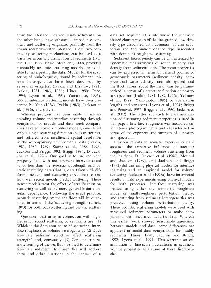
X-radiographs were made from specially de-signed rectangular cores that collected a 36-cmwideU3-cm thick sediment slab (P. Jackson etal., 1996). Sediment slabs were X-rayed within afew hours of collection with a model PX-20Nportable X-ray unit (Kramex, Saddle Brook, NJ,USA). Fig. 1 is an example of a positive imagemade from an X-radiograph. The light area indi-cating the overlying water clearly contrasts withthe lower, darker area signifying the sediment.Within the sediment appear relatively darkerand lighter features and zones, with dark areasrepresenting denser or less porous features (e.g.,shells, compact sediment) and light areas repre-senting less dense or more porous features (e.g.,burrows, reworked sediment).

For CT analysis, ¢ve 8.3-cm-diameter sedimentcores were collected throughout the study site.Scans were made of the whole, intact cores usingthe Technicare 2060 CT scanner at Texaco EpP,Houston, TX. The cores were scanned every2 mm, using a 2-mm-thick X-ray beam, to ensurecomplete length coverage with no overlap of im-

MARGO 2993 23-4-02

K.B. Briggs et al. / Marine Geology 182 (2002) 141^159 143

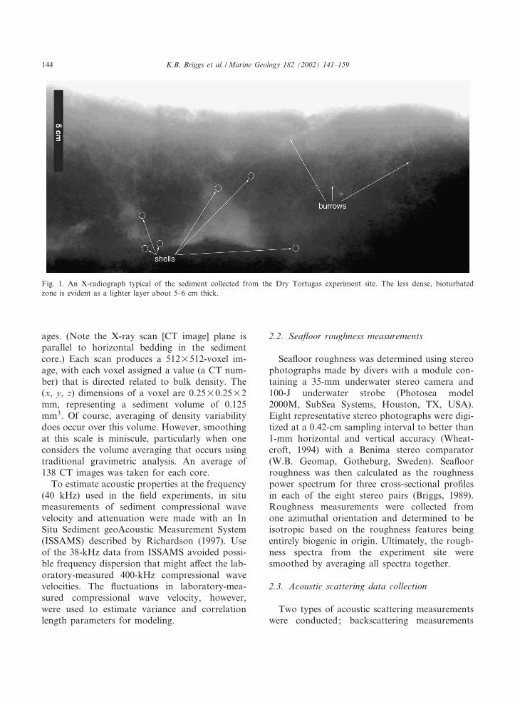
ages. (Note the X-ray scan [CT image] plane isparallel to horizontal bedding in the sedimentcore.) Each scan produces a 512U512-voxel im-age, with each voxel assigned a value (a CT num-ber) that is directed related to bulk density. The(x, y, z) dimensions of a voxel are 0.25U0.25U2mm, representing a sediment volume of 0.125mm3. Of course, averaging of density variabilitydoes occur over this volume. However, smoothingat this scale is miniscule, particularly when oneconsiders the volume averaging that occurs usingtraditional gravimetric analysis. An average of138 CT images was taken for each core.

To estimate acoustic properties at the frequency(40 kHz) used in the ¢eld experiments, in situmeasurements of sediment compressional wavevelocity and attenuation were made with an InSitu Sediment geoAcoustic Measurement System(ISSAMS) described by Richardson (1997). Useof the 38-kHz data from ISSAMS avoided possi-ble frequency dispersion that might a¡ect the lab-oratory-measured 400-kHz compressional wavevelocities. The £uctuations in laboratory-mea-sured compressional wave velocity, however,were used to estimate variance and correlationlength parameters for modeling.

2.2. Sea£oor roughness measurements

Sea£oor roughness was determined using stereophotographs made by divers with a module con-taining a 35-mm underwater stereo camera and100-J underwater strobe (Photosea model2000M, SubSea Systems, Houston, TX, USA).Eight representative stereo photographs were digi-tized at a 0.42-cm sampling interval to better than1-mm horizontal and vertical accuracy (Wheat-croft, 1994) with a Benima stereo comparator(W.B. Geomap, Gotheburg, Sweden). Sea£oorroughness was then calculated as the roughnesspower spectrum for three cross-sectional pro¢lesin each of the eight stereo pairs (Briggs, 1989).Roughness measurements were collected fromone azimuthal orientation and determined to beisotropic based on the roughness features beingentirely biogenic in origin. Ultimately, the rough-ness spectra from the experiment site weresmoothed by averaging all spectra together.

2.3. Acoustic scattering data collection

Two types of acoustic scattering measurementswere conducted; backscattering measurements

Fig. 1. An X-radiograph typical of the sediment collected from the Dry Tortugas experiment site. The less dense, bioturbatedzone is evident as a lighter layer about 5^6 cm thick.

MARGO 2993 23-4-02

K.B. Briggs et al. / Marine Geology 182 (2002) 141^159144

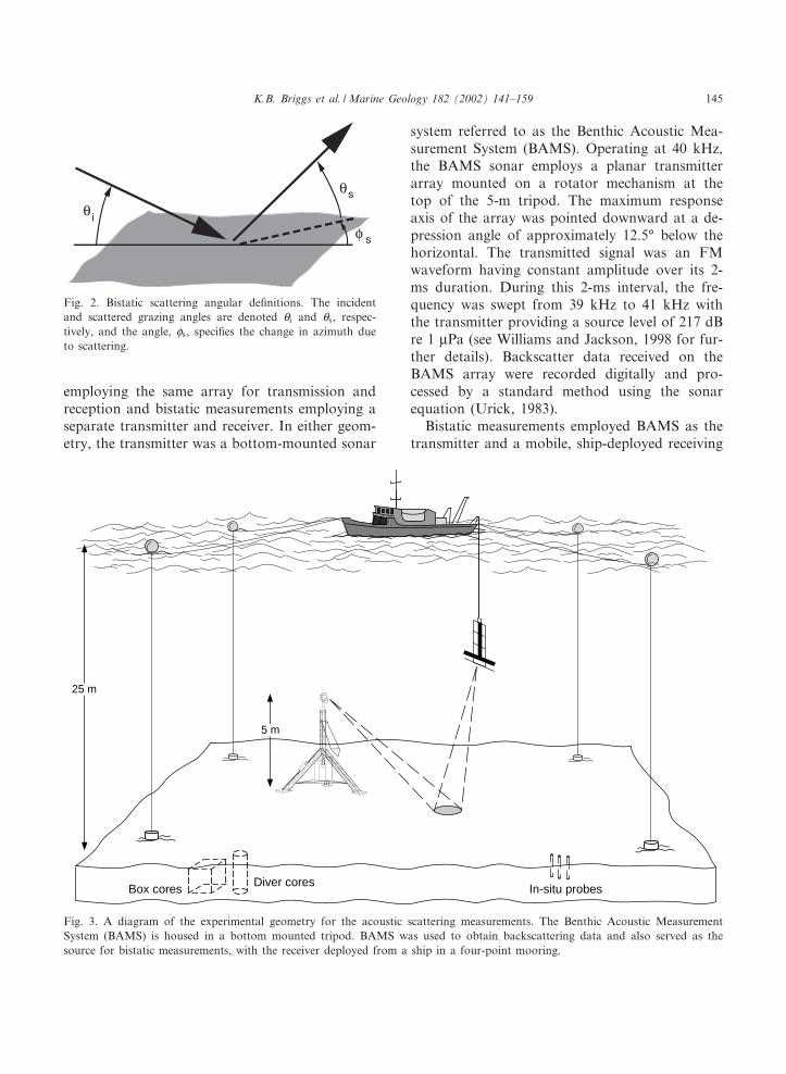
employing the same array for transmission andreception and bistatic measurements employing aseparate transmitter and receiver. In either geom-etry, the transmitter was a bottom-mounted sonar

system referred to as the Benthic Acoustic Mea-surement System (BAMS). Operating at 40 kHz,the BAMS sonar employs a planar transmitterarray mounted on a rotator mechanism at thetop of the 5-m tripod. The maximum responseaxis of the array was pointed downward at a de-pression angle of approximately 12.5‡ below thehorizontal. The transmitted signal was an FMwaveform having constant amplitude over its 2-ms duration. During this 2-ms interval, the fre-quency was swept from 39 kHz to 41 kHz withthe transmitter providing a source level of 217 dBre 1 WPa (see Williams and Jackson, 1998 for fur-ther details). Backscatter data received on theBAMS array were recorded digitally and pro-cessed by a standard method using the sonarequation (Urick, 1983).

Bistatic measurements employed BAMS as thetransmitter and a mobile, ship-deployed receiving

Diver coresBox cores In-situ probes

25 m

5 m

Fig. 3. A diagram of the experimental geometry for the acoustic scattering measurements. The Benthic Acoustic MeasurementSystem (BAMS) is housed in a bottom mounted tripod. BAMS was used to obtain backscattering data and also served as thesource for bistatic measurements, with the receiver deployed from a ship in a four-point mooring.

Fig. 2. Bistatic scattering angular de¢nitions. The incidentand scattered grazing angles are denoted ai and as, respec-tively, and the angle, Ps, speci¢es the change in azimuth dueto scattering.

MARGO 2993 23-4-02

K.B. Briggs et al. / Marine Geology 182 (2002) 141^159 145

array. Fig. 2 de¢nes the geometry of bistatic scat-tering by the sea £oor. Under the assumption thatthe sea£oor is transversely isotropic, as indicatedby analysis of the roughness data, a particulargeometry is speci¢ed by three angles, the incidentand scattered grazing angles, ai and as, and the‘bistatic’ angle, Ps, specifying the change in azi-muth due to scattering. The objective of theacoustic measurements was to cover as much ofthis three-dimensional angular space as practica-ble. As scattering by the sea£oor is a randomprocess, multiple measurements for each tripletof angles are required to obtain statistical aver-ages.

Fig. 3 shows a simpli¢ed diagram of the bistaticexperimental geometry. The ship-deployed linear,horizontal, receiving array was divided in fourequal sections (‘quads’) each about 32 cm long.The bistatic scattering results reported here wereacquired using a single quad at two di¡erent gainsto increase dynamic range. The array was de-ployed over the side of the ship after it was placedin a four-point moor near the BAMS tripod, anda pneumatic heave compensation system was usedto decouple the ship’s aft deck motion from thearray. The receiving array was steered so that thecenter of the transmit and receive beams inter-sected each other on the bottom such as to realize

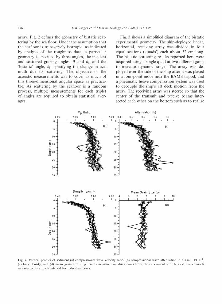
Fig. 4. Vertical pro¢les of sediment (a) compressional wave velocity ratio, (b) compressional wave attenuation in dB m31 kHz31,(c) bulk density, and (d) mean grain size in phi units measured on diver cores from the experiment site. A solid line connectsmeasurements at each interval for individual cores.

MARGO 2993 23-4-02

K.B. Briggs et al. / Marine Geology 182 (2002) 141^159146

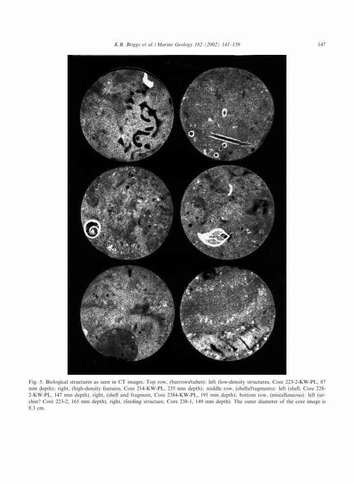
Fig. 5. Biological structures as seen in CT images. Top row, (burrows/tubes): left (low-density structures, Core 223-2-KW-PL, 87mm depth); right, (high-density features, Core 214-KW-PL, 235 mm depth); middle row, (shells/fragments): left (shell, Core 228-2-KW-PL, 147 mm depth), right, (shell and fragment, Core 2384-KW-PL, 191 mm depth); bottom row, (miscellaneous): left (ur-chin? Core 223-2, 165 mm depth), right, (feeding structure, Core 238-1, 149 mm depth). The outer diameter of the core image is8.3 cm.

MARGO 2993 23-4-02

K.B. Briggs et al. / Marine Geology 182 (2002) 141^159 147

di¡erent bistatic scattering angles, de¢ned in Fig. 2(see Williams and Jackson, 1998 for further de-tails).

Measuring the geometrical parameters neededto determine these bistatic angles required severalsupplemental sensors including compasses, rang-ing transducers, and inclinometers. The rangefrom BAMS to the mobile array was measuredby means of a transponder mounted on the tri-pod. In the data to be presented the horizontaldistance between BAMS and the receiving arraywas always less than 70 m.

While backscattering strength is easily esti-mated using the sonar equation owing to the sim-ple correspondence between acoustic time-of-£ight and backscattering angle, it is much moredi⁄cult to estimate bistatic scattering strength. Toaid in this process, a simulation was developedthat predicts the mean-square output of the re-ceiver array as a function of time (Williams andJackson, 1998) using the ‘baseline’ model for scat-tering, to be discussed in Section 4. Using exper-imentally determined geometric parameters, thesimulation was used to produce a syntheticmean-square receiver output time series for eachtransmission. This synthetic time series was thencompared with the data time series to determinethe experiment bistatic scattering strength (Wil-liams and Jackson, 1998).

3. Results

3.1. Geoacoustic data

Fig. 4 displays the vertical distribution of sedi-ment compressional wave velocity ratio, attenua-tion, density, and mean grain size for ten cores(only seven cores were assessed for grain size)collected from within the acoustic experimentsite in the Dry Tortugas. The variability and num-ber of measurements of each parameter aregraphically indicated by the plotted symbols. In-dividual lines connecting the symbols indicate var-iation within individual cores. Although morecores were collected in the experiment (D. Jack-son et al., 1996), only the longest ones were chos-en for this study. Variability of sediment compres-

sional wave velocity, attenuation, grain size, andto a lesser extent, sediment density is controlledby the presence of burrows and coarse shell frag-ments within the sediment matrix (Briggs and Ri-chardson, 1997; Richardson et al., 1997). The X-radiograph in Fig. 1 shows that burrows and mol-lusk shell fragments are prominent in sedimentsfrom the Dry Tortugas site.

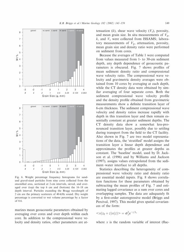
In accordance with radiographic and gravimet-ric analyses (Figs. 1 and 4), CT imagery of theDry Tortugas cores revealed considerable inho-mogeneity, with the dominant source of this var-iability being biological in origin (Fig. 5). Partic-ularly prevalent are tubes and burrows, with wallscomposed of both low- and high-density material,which generate localized structures easily detectedand quanti¢ed by CT. Present but less commonare shells and shell debris. Large intact gastropodshells occur (Fig. 5), whereas the shell fragmentsthat we observe are probably derived from brokenpelecypods. Most of the gastropod shells are sedi-ment-¢lled, but several contain pockets of water(or sediment^water slurry) that could result inconsiderable intratest porosity. Acoustically, shellfragments of 2-cm diameter and larger are ex-pected to be most signi¢cant as ‘Bragg’ scatterersat the 40-kHz frequency utilized here. The distri-bution of 2-cm particles in the upper 30 cm ofsediment, however, is extremely sparse (Fig. 6).Grain-size analysis of eight cores showed no frag-ments larger than 33.25 P diameter (9.5 mm). Ina total sediment volume of 6.605 l, however, wefound average weight fractions of 1.8% (71 ml ofcalcium carbonate) for fragments larger than33.0 P diameter (8 mm) at 17 cm depth (Fig. 6,bottom) but less than 0.1% (3.6 ml of calciumcarbonate) for all gravel-size fragments largerthan 31.0 P diameter (2 mm) in the top 6 cm(Fig. 6, top). The CT imagery reveals several largefeeding structures, possibly created by foragingheart urchins or some other type of large macro-fauna.

The compressional wave velocity (Vp) ratio isan important acoustic model parameter obtainedby dividing the sound velocity in the sediment bythe sound velocity in the overlying water. Thedensity ratio is the analogous ratio of sedimentdensity to overlying water density. Table 1 sum-

MARGO 2993 23-4-02

K.B. Briggs et al. / Marine Geology 182 (2002) 141^159148

marizes mean geoacoustic parameters obtained byaveraging over cores and over depth within eachcore. In addition to the compressional wave ve-locity and density ratios, other parameters are at-

tenuation (k), shear wave velocity (Vs), porosity,and mean grain size. In situ measurements of Vp,k, and Vs were collected from ISSAMS; labora-tory measurements of Vp, attenuation, porosity,mean grain size and density ratio were performedon sediment from cores.

Because the averages of Table 1 were computedfrom values measured from 1- to 30-cm sedimentdepth, any depth dependence of geoacoustic pa-rameters is obscured. Fig. 7 shows pro¢les ofmean sediment density ratio and compressionalwave velocity ratio. The compressional wave ve-locity and gravimetric density averages were ob-tained from 10 cores by averaging at each depth,while the CT density data were obtained by sim-ilar averaging of four separate cores. Both thesediment compressional wave velocity pro¢leand the density pro¢le obtained from gravimetricmeasurements show a de¢nite transition layer of6-cm thickness. The sediment compressional wavevelocity and density ratios increase rapidly withdepth in this transition layer and then remain es-sentially constant at greater sediment depths. TheCT density data show a somewhat less-pro-nounced transition layer, possibly due to settlingduring transport from the ¢eld to the CT facility.Also shown in Fig. 7 are two model representa-tions of the data, the ‘strati¢ed’ model assigns thetransition layer a linear depth dependence andapproximates the pro¢les at greater depths asconstant. The ‘baseline’ model, used by D. Jack-son et al. (1996) and by Williams and Jackson(1997), assigns values extrapolated from the sedi-ment^water interface to all depths.

Statistics describing the heterogeneity of com-pressional wave velocity ratio and density ratioare essential model inputs. Fig. 8 shows correla-tion functions for these parameters obtained bysubtracting the mean pro¢les of Fig. 7 and esti-mating lagged covariance as a sum over cores andoverlapping samples. The data are adequately ¢tby a ¢rst-order autoregressive model (Briggs andPercival, 1997). This model gives spatial covarian-ces of the form:

6xðz0 þ zÞxðzÞs ¼ c2xe3z=1c

where x is the random variable of interest (£uc-

Fig. 6. Weight percentage frequency histograms for sand-and gravel-sized particles from nine cores collected from theensoni¢ed area, sectioned at 2-cm intervals, sieved, and aver-aged over (top) the top 6 cm and (bottom) the 16^18 cmdepth interval. Particles exceeding the Bragg wavelength of2 cm are the primary scatterers of 40-kHz sound. Dry weightpercentage is converted to wet volume percentage by a factorof 0.6.

MARGO 2993 23-4-02

K.B. Briggs et al. / Marine Geology 182 (2002) 141^159 149

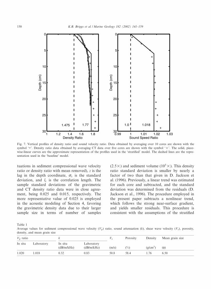
tuations in sediment compressional wave velocityratio or density ratio with mean removed), z is thelag in the depth coordinate, cx is the standarddeviation, and lc is the correlation length. Thesample standard deviations of the gravimetricand CT density ratio data were in close agree-ment, being 0.025 and 0.015, respectively. Themore representative value of 0.025 is employedin the acoustic modeling of Section 4, favoringthe gravimetric density data due to their largersample size in terms of number of samples

(2.5U) and sediment volume (105U). This densityratio standard deviation is smaller by nearly afactor of two than that given in D. Jackson etal. (1996). Previously, a linear trend was estimatedfor each core and subtracted, and the standarddeviation was determined from the residuals (D.Jackson et al., 1996). The procedure employed inthe present paper subtracts a nonlinear trend,which follows the strong near-surface gradient,and yields smaller residuals. This procedure isconsistent with the assumptions of the strati¢ed

Table 1Average values for sediment compressional wave velocity (Vp) ratio, sound attenuation (k), shear wave velocity (Vs), porosity,density, and mean grain size

Vp ratio k Vs Porosity Density Mean grain size

In situ Laboratory In situ Laboratory(dB/m/kHz) (dB/m/kHz) (m/s) (%) (g/cm3) (P)

1.020 1.018 0.32 0.83 50.8 58.4 1.76 6.50

Fig. 7. Vertical pro¢les of density ratio and sound velocity ratio. Data obtained by averaging over 10 cores are shown with thesymbol ‘+’. Density ratio data obtained by averaging CT data over ¢ve cores are shown with the symbol ‘U’. The solid, piece-wise-linear curves are the approximate representation of the pro¢les used in the ‘strati¢ed’ model. The dashed lines are the repre-sentation used in the ‘baseline’ model.

MARGO 2993 23-4-02

K.B. Briggs et al. / Marine Geology 182 (2002) 141^159150

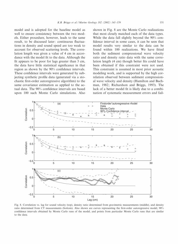
model and is adopted for the baseline model aswell to ensure consistency between the two mod-els. Either procedure, however, leads to the sameresult, to be discussed later: continuous £uctua-tions in density and sound speed are too weak toaccount for observed scattering levels. The corre-lation length was given a value of 4 cm in accor-dance with the model ¢t to the data. Although the¢t appears to be poor for lags greater than 5 cm,the data have little statistical signi¢cance in thatregion as shown by the 90% con¢dence intervals.These con¢dence intervals were generated by sub-jecting synthetic pro¢le data (generated via a sto-chastic ¢rst-order autoregressive algorithm) to thesame covariance estimation as applied to the ac-tual data. The 90% con¢dence intervals are basedupon 100 such Monte Carlo simulations. Also

shown in Fig. 8 are the Monte Carlo realizationsthat most closely matched each of the data types.While the data fall slightly beyond the 90% con-¢dence interval in some cases, it can be seen thatmodel results very similar to the data can befound within 100 realizations. We have ¢ttedboth the sediment compressional wave velocityratio and density ratio data with the same corre-lation length (4 cm) though better ¢ts could havebeen obtained if this constraint were not used.This constraint is assumed in most prior acousticmodeling work, and is supported by the high cor-relation observed between sediment compression-al wave velocity and density (Hamilton and Bach-man, 1982; Richardson and Briggs, 1993). Thelack of a better model ¢t is likely due to a combi-nation of systematic measurement errors and fail-

Fig. 8. Correlation vs. lag for sound velocity (top), density ratio determined from gravimetric measurements (middle), and densityratio determined from CT measurements (bottom). Also shown are curves representing the ¢rst-order autoregressive model, 90%con¢dence intervals obtained by Monte Carlo runs of the model, and points from particular Monte Carlo runs that are similarto the data.

MARGO 2993 23-4-02

K.B. Briggs et al. / Marine Geology 182 (2002) 141^159 151

ure of the data to conform to the ¢rst-order au-toregressive model. Two possible sources of sys-tematic error are alteration of sediment propertiesin the course of core sampling and smearing ofdata due to ¢nite spatial resolution. The CT andsediment compressional wave velocity data haveapproximate resolutions of 2 mm and 1 cm, re-spectively, while the gravimetric data have 2-cmresolution. The CT and sediment compressionalwave velocity data were in close agreement withregard to correlation length and were thereforegiven priority in the ¢t to determine correlationlength. This ¢tting process simply consisted in ad-justment of the correlation length of the MonteCarlo model to the point where the CT and ve-locity data remained within the 90% con¢denceinterval in the 0^5-cm lag region while the gravi-metric data were at the lower edge of this interval.The Monte Carlo simulations show that the au-toregressive model is satisfactory for scales of2 mm to 5 cm but also shows that the data areinsu⁄cient to support this model at longer scales.This is not a problem in the present context as theacoustic wavelength is about 3.8 cm and scalessigni¢cantly larger do not play a prominent rolein scattering, at least in the perturbation modelsemployed here.

To conclude, the availability of high resolutionCT density data has con¢rmed previous estimatesof sediment £uctuation statistics with a minormodi¢cation: the correlation length appears tobe closer to 4 cm than to 3 cm, the previouslyreported estimate (D. Jackson et al., 1996),although the older value is within the errorbounds set by Monte Carlo simulations.

3.2. Stereo photogrammetric data

The averaged roughness power spectrum forthe sea £oor at the experiment site appeared to¢t a linear regression of log spectral density (dBcm3) on log spatial frequency (1/cm) of slope32.29 and intercept 2.092U1033 cm3 (Jacksonet al., 1996a). The averaged power spectrum,which spanned a spatial wavelength range fromless than a cm to just beyond 53 cm, fell withinthe 95% statistical con¢dence limits of the regres-sion line except at spatial wavelengths above 25

cm and near 4 cm. Because the largest deviationfrom the power-law ¢t exists at the longest wave-lengths and is consistent with spectrum ‘roll o¡’ atlow spatial frequency (Briggs, 1989), the power-law ¢t is judged to be quite reasonable. Mostimportantly, the measured spectra include infor-mation at the high spatial frequencies of acousticinterest corresponding to the Bragg wavelengthnear 2 cm and beyond.

The roughness spectrum is sensitive to subtledi¡erences in microtopography. This sensitivitywas demonstrated at the experiment site by re-measuring roughness from the same sea £oorafter being physically smoothed by divers. Thespectrum calculated from the physically alteredsea £oor had a statistically steeper slope (32.60)and a depressed intercept (0.725U1033 cm3) as aresult of the lack of high spatial-frequency rough-ness. The two average spectra were shown to besigni¢cantly di¡erent by an analysis of covariancethat tests the di¡erence between the slopes of theregression lines (Sokal and Rohlf, 1969). Eachregression ¢t was made from 24 measurementsand tested at the K6 0.05 level of signi¢cance.

3.3. Acoustic data

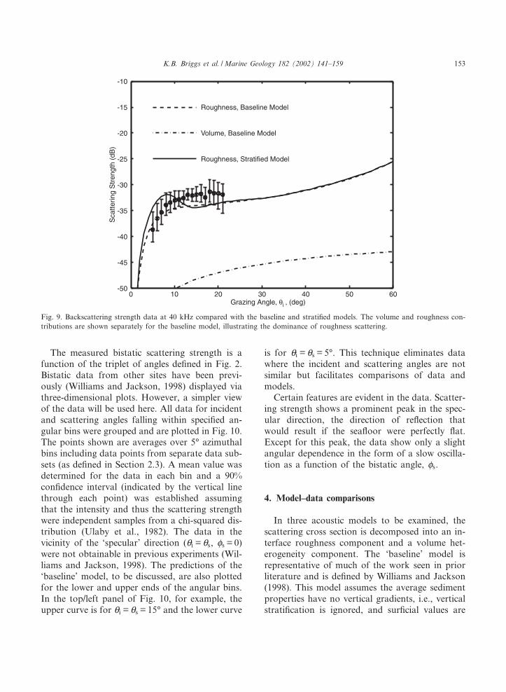
The acoustic measurements include both mono-static and bistatic geometry. The monostatic ge-ometry, with transmitter and receiver at the samelocation, produced the scattering strength datashown in Fig. 9. These data are averages over asingle scan of the BAMS system, taken beforeobjects were placed on the sea£oor as part of atarget scattering study. Averaging included theentire 360‡ scan interval, as no anisotropy wasevident in the data. Together with the baselinemodel curve shown, Fig. 9 replicates the model^data comparison reported in Jackson et al.(1996a) except for a slight shift in the data result-ing from improved directivity corrections in pro-cessing. The vertical bars indicate systematic er-rors due to possible 1‡ uncertainty in arraypointing angle and 2-dB uncertainty in transducersensitivity and receiver gain. Statistical errors andother known systematic errors are smaller and arenot shown. The baseline model and other modelswill be discussed in Section 4.

MARGO 2993 23-4-02

K.B. Briggs et al. / Marine Geology 182 (2002) 141^159152

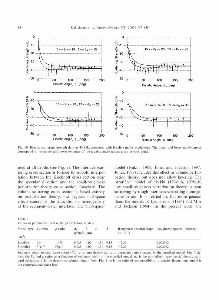
The measured bistatic scattering strength is afunction of the triplet of angles de¢ned in Fig. 2.Bistatic data from other sites have been previ-ously (Williams and Jackson, 1998) displayed viathree-dimensional plots. However, a simpler viewof the data will be used here. All data for incidentand scattering angles falling within speci¢ed an-gular bins were grouped and are plotted in Fig. 10.The points shown are averages over 5‡ azimuthalbins including data points from separate data sub-sets (as de¢ned in Section 2.3). A mean value wasdetermined for the data in each bin and a 90%con¢dence interval (indicated by the vertical linethrough each point) was established assumingthat the intensity and thus the scattering strengthwere independent samples from a chi-squared dis-tribution (Ulaby et al., 1982). The data in thevicinity of the ‘specular’ direction (ai = as, Ps = 0)were not obtainable in previous experiments (Wil-liams and Jackson, 1998). The predictions of the‘baseline’ model, to be discussed, are also plottedfor the lower and upper ends of the angular bins.In the top/left panel of Fig. 10, for example, theupper curve is for ai = as = 15‡ and the lower curve

is for ai = as = 5‡. This technique eliminates datawhere the incident and scattering angles are notsimilar but facilitates comparisons of data andmodels.

Certain features are evident in the data. Scatter-ing strength shows a prominent peak in the spec-ular direction, the direction of re£ection thatwould result if the sea£oor were perfectly £at.Except for this peak, the data show only a slightangular dependence in the form of a slow oscilla-tion as a function of the bistatic angle, Ps.

4. Model^data comparisons

In three acoustic models to be examined, thescattering cross section is decomposed into an in-terface roughness component and a volume het-erogeneity component. The ‘baseline’ model isrepresentative of much of the work seen in priorliterature and is de¢ned by Williams and Jackson(1998). This model assumes the average sedimentproperties have no vertical gradients, i.e., verticalstrati¢cation is ignored, and sur¢cial values are

Fig. 9. Backscattering strength data at 40 kHz compared with the baseline and strati¢ed models. The volume and roughness con-tributions are shown separately for the baseline model, illustrating the dominance of roughness scattering.

MARGO 2993 23-4-02

K.B. Briggs et al. / Marine Geology 182 (2002) 141^159 153

used at all depths (see Fig. 7). The interface scat-tering cross section is formed by smooth interpo-lation between the Kirchho¡ cross section nearthe specular direction and the small-roughnessperturbation-theory cross section elsewhere. Thevolume scattering cross section is based entirelyon perturbation theory, but neglects half-spacee¡ects caused by the truncation of heterogeneityat the sediment^water interface. The ‘half-space’

model (Ivakin, 1984; Jones and Jackson, 1997;Jones, 1999) includes this e¡ect in volume pertur-bation theory, but does not allow layering. The‘strati¢ed’ model of Ivakin (1994a,b, 1998a,b)uses small-roughness perturbation theory to treatscattering by rough interfaces separating homoge-neous strata. It is related to, but more generalthan, the models of Lyons et al. (1994) and Moeand Jackson (1994). In the present work, the

Table 2Values of parameters used in the perturbation models

Model type Vp ratio b ratio cb lc W N Roughness spectral slope Roughness spectral intercept(g/cm3) (cm) (U1033)

(cm3)

Baseline 1.0 1.475 0.025 4.00 31.31 9.15 32.29 0.002092Strati¢ed Fig. 7 Fig. 7 0.025 4.00 31.31 9.15 32.29 0.002092

Sediment compressional wave speed (Vp) ratio, and density (b) ratio parameters are changed in the strati¢ed model. Fig. 7 de-picts the Vp and b ratios as a function of sediment depth in the strati¢ed model. cb is the normalized (gravimetric) density stan-dard deviation, lc is the density correlation length from Fig. 8, W is the ratio of compressibility to density £uctuations and N isthe compressional wave loss.

Fig. 10. Bistatic scattering strength data at 40 kHz compared with baseline model predictions. The upper and lower model curvescorrespond to the upper and lower extremes of the grazing angle ranges given in each panel.

MARGO 2993 23-4-02

K.B. Briggs et al. / Marine Geology 182 (2002) 141^159154

piecewise linear ¢ts to compressional wave veloc-ity ratio and density ratio shown in Fig. 7 areused as inputs (Table 2). All other parametersare assumed to be depth independent. In thecase of compressional wave loss (N) this assump-tion is reasonable, as the model is rather insensi-tive to this parameter. In the case of £uctuationstatistics, this assumption is dictated by the lackof su⁄cient data to estimate depth dependence.The models require an additional parameter, W,the ratio of compressibility £uctuations to density£uctuations, which are assumed to be perfectlycorrelated. We adopt the depth-independent valueW= -1.31 calculated by D. Jackson et al. (1996).

4.1. Baseline model

For the baseline model, which cannot deal withstrati¢cation, the compressional wave velocity anddensity ratios were assigned the sur¢cial values of1.0 and 1.475, respectively (Fig. 7). A comparison

of this model with backscattering data shows thatthe model matches the level of scattering within afew dB but shows less dependence on grazing an-gle than the data (Fig. 9). Two curves are shownfor the baseline model, one representing the con-tribution of volume scattering and the other giv-ing the contribution of roughness scattering. Itcan be seen that the model predicts that rough-ness scattering is dominant. Fig. 10 compares thebaseline model with bistatic scattering data. Aninitial examination of Fig. 10 indicates good over-all agreement between the data and the baselinemodel. Close inspection of Fig. 10, however, re-veals small but systematic di¡erences. First, thedata points in the top/right panel seem to havean oscillation not seen in the model in the region70‡6 P6 180‡. Second, in the same panel, themodel seems to overpredict the scattering crosssection in the region 30‡6 P6 70‡. Finally, thereis some indication in the bottom two panels thatthe model underpredicts the scattering in the re-

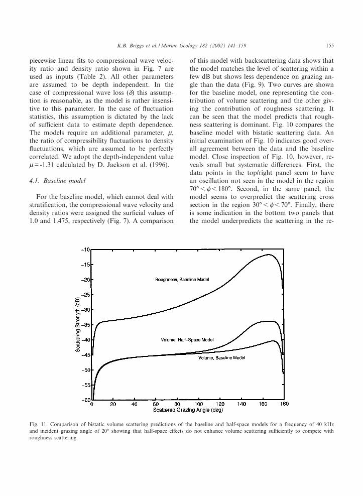
Fig. 11. Comparison of bistatic volume scattering predictions of the baseline and half-space models for a frequency of 40 kHzand incident grazing angle of 20‡ showing that half-space e¡ects do not enhance volume scattering su⁄ciently to compete withroughness scattering.

MARGO 2993 23-4-02

K.B. Briggs et al. / Marine Geology 182 (2002) 141^159 155

gion 130‡6 P6 180‡ for the higher grazing anglesof those panels. It is worthwhile to remember thatthe model has no free parameters, but these di¡er-ences may indicate that some details of scatteringare not properly modeled.

4.2. Half-space model

Because the baseline model neglects half-spacee¡ects in its treatment of volume scattering, wecompare the baseline and half-space space modelsfor bistatic scattering (Fig. 11). Although half-space e¡ects elevate the volume scattering contri-bution near the specular direction, the e¡ect is toosmall to compensate for the dominance of inter-face scattering. This supports the earlier conclu-sion of D. Jackson et al. (1996). Dominance ofinterface scattering at this site is rather surprising,given the low bulk density of the sediment, typicalof silty mud. However, it should be mentionedthat the spectral strength of volume £uctuationsin this site was found to be relatively weak in

comparison with that in other sites covered byanalogous types of sediments (see, e.g., Ye¢movet al., 1988) and having signi¢cant volume scatter-ing.

4.3. Strati¢ed model

If volume scattering is negligible, the modestdiscrepancies between the baseline model andthe data may lie in the treatment of roughnessscattering. It is possible that interference e¡ectscaused by refraction in the upper layer of the sedi-ment cause oscillations in the angular dependenceof scattering strength (Ivakin, 1986, 1989,1994a,b, 1998b; Moe and Jackson, 1994). Fig. 9includes a curve for the strati¢ed model in thebackscattering case. The slight angular ‘bump’ isindeed a result of interference, but it worsens,rather than improves, the model^data ¢t. Wehave also considered scattering from the interfaceat 6-cm depth, but plausible guesses at the rough-ness of this interface fall far short of changing the

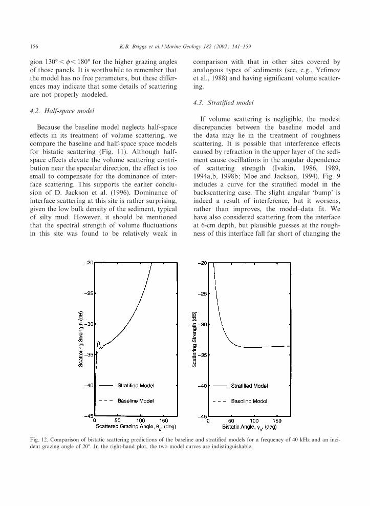
Fig. 12. Comparison of bistatic scattering predictions of the baseline and strati¢ed models for a frequency of 40 kHz and an inci-dent grazing angle of 20‡. In the right-hand plot, the two model curves are indistinguishable.

MARGO 2993 23-4-02

K.B. Briggs et al. / Marine Geology 182 (2002) 141^159156

model prediction. This is because there is littleacoustic contrast across this interface. The back-scattering bump is a robust feature of the strati-¢ed model that persists when model predictionsare averaged over likely lateral variations in pa-rameters or when details of the vertical pro¢lesfor density and sound velocity ratios are alteredwithin experimental uncertainty.

Fig. 12 compares the baseline model with thestrati¢ed model for the bistatic case. According tothe model, the observed strati¢cation has littlee¡ect on bistatic scattering and does not causeoscillations with respect to the bistatic angle.

5. Discussion

The CT data have led to a re¢nement in thegeoacoustic model originally developed for theDry Tortugas site, but the resulting acoustic pre-dictions are changed very little, even when thee¡ects of strati¢cation are included. This outcomeis signi¢cant because it implies that the inverse istrue: acoustic sensing of the sea £oor at this fre-quency would not provide de¢nition of the ¢ne-scale £uctuations of the geoacoustic properties inthe sediment volume. The primary modeling re-sult is that scattering due to roughness of the sedi-ment^water interface dominates scattering due tovolume heterogeneity, as de¢ned here. Althoughthe acoustic models match the data reasonablywell in terms of scattering level and approximateangular dependence, certain details in the data aremarginally di¡erent than the model predictions. Itshould be noted that the volume scattering com-ponent of the model considered here only treatscontinuous spatial variations in sediment com-pressional wave speed and density. Such varia-tions in these parameters are due to the presenceof burrow structures, open (water-¢lled) or in¢lledwith sediment. Coarse skeletal material (i.e., mol-lusk shells, urchin tests, coral rubble), however, isanother likely source of scattering that may notbe adequately characterized by ¢ne-scale measure-ments of sediment compressional wave speed anddensity. Scattering due to discrete carbonate frag-ments has not been considered, but a crude cal-culation shows that a shallow layer of 10^20 gas-

tropod shells per m2 of the size seen in the CTimages could compete with interface roughness asa source of backscattered energy. This type ofscattering would tend to ‘¢ll in’ angular regionswhere interface scattering is relatively weak. Insuch a scenario, scattering from shells might ob-scure the bump predicted by the strati¢ed model.Discrete scatterers should be considered in futuremodeling e¡orts (see Bunchuk and Ivakin, 1989).

It is the generation and maintenance of biogen-ic structures such as burrows that control thephysical and acoustic properties of the sedimentat Dry Tortugas. Localized, time-dependent var-iations in acoustic backscattering intensity havebeen linked with measurements of changing po-rosity (and thus density) and sound velocity(Briggs and Richardson, 1997). Moreover, X-ra-diographs of these areas of dilated sediment dis-play burrow networking and presence of burrow-ing crustaceans. Because these burrowers areoperationally restricted to the uppermost 5^10cm of sediment, their reworking activities createand maintain a pronounced gradient in sedimentdensity and, consequently, sediment sound veloc-ity as depicted in Fig. 4. The time scale overwhich decorrelation of acoustic backscattering re-sponse due to bioturbation occurs at any partic-ular spot at Dry Tortugas is on the order of 2 daysand the decorrelation within the ensoni¢ed areais about 23^24% complete after 2.25 days (see¢g. 8 in Briggs and Richardson, 1997). Thus, thetop few cm of sediment throughout the area ofstudy are reworked to an acoustically detectableextent in the course of weeks. The dynamic natureof the sea £oor as a result of intensive bioturba-tion may provide the strong gradient capable ofrefracting acoustic energy and creating interfer-ence e¡ects in the model (though not seen in thedata).

Furthermore, the intensive reworking of thesediment by burrowing organisms is generatingthe interface roughness that is the dominant causeof acoustic scattering from the sea £oor. Fromdiver observations as well as stereo photogram-metry, the distinguishing roughness features areidenti¢ed as the sediment mounds created bycrustaceans, polychaete worms, and heart urchins(D’Andrea and Lopez, 1997). Although the mean

MARGO 2993 23-4-02

K.B. Briggs et al. / Marine Geology 182 (2002) 141^159 157

height of the biogenic roughness features is mod-est (0.66 cm) and the sediment comprising thevolcano-shaped mounds that predominate amongthe roughness features necessarily has a low bulkdensity, the grain density of carbonate skeletalmaterial is relatively high (mean: 2.76 g/cm3)(Wright et al., 1997; Stephens et al., 1997). Ap-parently, this reworked sediment provides enoughimpedance contrast with the overlying water toaccount for the dominance of interface scatteringover volume scattering.

With regard to inversions to determine sedi-ment properties, our results show that scatteringis sensitive to sur¢cial properties (density andsound velocity). Although the modeling resultsindicate that strati¢cation should be evident in asmall but persistent backscattering feature, thisfeature is not seen and may be obscured by scat-tering due to shells. The contribution that shellsand shell fragments make to acoustic scattering,however, is not quanti¢ed adequately by sedimentsound speed and bulk density measurements, evenat relatively high resolution (2 mm).

Acknowledgements

We wish to thank Michael Richardson, RichardRay, David Young, Nancy Carnaggio, and KevinShea for help in the shipboard and/or laboratoryoperations. Russell Light, Le Olsen, and VernMiller were responsible for the design and deploy-ment of the acoustic apparatus. This work wasfunded by the Coastal Benthic Boundary Layerprogram sponsored by the Office of NavalResearch, Program Element No. 601153N, man-aged by the Naval Research Laboratory, M.D.Richardson, chief scientist. The work of A.N.Ivakin was funded by the Office of NavalResearch. The NRL contribution number isNRL/JA/7431-00-0008.

References

Brandes, H.G., Silva, A.J., Walter, D.J., 2002. Geo-acousticcharacterization of calcareous seabed in the Florida Keys.Mar. Geol., this issue.

Briggs, K.B., 1989. Microtopographical roughness of shallow-water continental shelves. IEEE J. Oceanic Eng. 14, 360^367.

Briggs, K.B., 1994. High frequency acoustic scattering fromsediment interface roughness and volume inhomogeneities.Ph.D. dissertation, University of Miami, Coral Gables, FL,143 pp.

Briggs, K.B., Percival, D.B., 1997. Vertical porosity and veloc-ity £uctuations in shallow-water sur¢cial sediments and theiruse in modeling volume scattering. In: Pace, N.G., Pouli-quen, E., Bergem, O., Lyons, A.P. (Eds.), High FrequencyAcoustics in Shallow Water. NATO SACLANT UnderseaRes. Ctr., La Spezia, pp. 65^73.

Briggs, K.B., Richardson, M.D., 1997. Small-scale £uctuationsin acoustic and physical properties in sur¢cial carbonatesediments and their relationship to bioturbation. GeoMar.Lett. 17, 306^315.

Briggs, K.B., Jackson, P.D., Holyer, R.J., Flint, R.C., San-didge, J.C., Young, D.K., 1998. Two-dimensional variabilityin porosity, density, and electrical resistivity in Eckernfo«rdeBay sediment. Cont. Shelf Res. 18, 1939^1964.

Bunchuk, A.V., Ivakin, A.N., 1989. Energy characteristics ofan echo signal from discrete scatterers on the ocean bottom.Sov. Phys. Acoust. 35, 5^11.

D’Andrea, A.F., Lopez, G.R., 1997. Benthic macrofauna in ashallow water carbonate sediment: major bioturbators at theDry Tortugas. GeoMar. Lett. 17, 276^282.

Hamilton, E.L., Bachman, R.T., 1982. Sound velocity andrelated properties of marine sediments. J. Acoust. Soc.Am. 72, 1891^1904.

Hines, P.C., 1990. Theoretical model of acoustic backscatter-ing from a smooth seabed. J. Acoust. Soc. Am. 88, 325^334.

Ivakin, A.N., Lysanov, Yu.P., 1981. Theory of underwatersound scattering by random inhomogeneities of the bottom.Sov. Phys. Acoust. 27, 61^64.

Ivakin, A.N., 1981. Sound scattering by multi-scale bottominhomogeneities. Oceanology 21, 26^27.

Ivakin, A.N., 1982. Sound Scattering and Re£ection by Inho-mogeneities of a Seabed. Ph.D. Thesis, Andreev AcousticsInstitute, Moscow (in Russian).

Ivakin, A.N., 1983. Sound scattering by random volume inho-mogeneities and small surface roughness and of underwaterground, Voprosy sudostroeniya (in Russian). Akustika 17,20^25.

Ivakin, A.N., 1984. Sound scattering by volume inhomogene-ities of strongly absorbing media. Andreev Acoust. Inst. Sci.Report (in Russian).

Ivakin, A.N., 1986. Sound scattering by random inhomogene-ities of strati¢ed ocean sediments. Sov. Phys. Acoust. 32,492^496.

Ivakin, A.N., 1989. Backscattering of sound by the ocean bot-tom. Theory and experiment. In: Brekhovskikh, L.M., An-dreeva, I.B. (Eds.), Acoustics of the Ocean Medium. Nauka,Moscow, pp. 160^169 (in Russian).

Ivakin, A.N., 1994a. Modelling of sound scattering by the sea£oor. J. Phys. IV Coll. C5 4, 1095^1098.

Ivakin, A.N., 1994b. Sound scattering by rough interfaces of

MARGO 2993 23-4-02

K.B. Briggs et al. / Marine Geology 182 (2002) 141^159158

layered media. In: Crocker, M.J. (Ed.), Third InternationalCongress on Air- and Structure-Borne Sound and Vibration,International Publications, Auburn University, vol. 3, pp.1563^1570.

Ivakin, A.N., 1998a. A uni¢ed approach to volume and rough-ness scattering. J. Acoust. Soc. Am. 103, 827^837.

Ivakin, A.N., 1998b. Models of sea£oor roughness and volumescattering. In: Proc. Oceans ’98, IEEE Publ. No.98CH36259, vol. 1, pp. 518^521.

Ivakin, A.N., 1998c. Models for acoustic scattering from theocean bottom: State of the art. In: Brekhovskikh, L.M.(Ed.), School-Seminar, Ocean Acoustics. GEOS, Moscow,pp. 84^91 (in Russian).

Jackson, D.R., Winebrenner, D.P., Ishimaru, A., 1986. Appli-cation of the composite roughness model to high-frequencybottom backscattering. J. Acoust. Soc. Am. 79, 1410^1422.

Jackson, D.R., Briggs, K.B., 1992. High-frequency bottombackscattering: roughness vs. sediment volume scattering.J. Acoust. Soc. Am. 92, 962^977.

Jackson, D.R., Briggs, K.B., Williams, K.L., Richardson,M.D., 1996. Tests of models for high-frequency sea-£oorbackscatter. IEEE J. Oceanic Eng. 21, 458^470.

Jackson, P.D., Briggs, K.B., Flint, R.C., 1996. Evaluation ofsediment heterogeneity using micro-resistivity imaging andX-radiography. GeoMar. Lett. 16, 219^226.

Jackson, P.D., Flint, R.C., Briggs, K.B., Holyer, R.J. andSandidge, J.C., 2002. Two- and three-dimensional heteroge-neity in carbonate sediments using resistivity imaging. Mar.Geol., this issue.

Jones, C.D., Jackson, D.R., 1997. Temporal £uctuations ofbackscattered ¢eld due to bioturbation in marine sediments.In: Pace, N.G., Pouliquen, E., Bergem, O., Lyons, A.P.(Eds.), High Frequency Acoustics in Shallow Water.NATO SACLANT Undersea Res. Ctr., La Spezia, pp.275^282.

Jones, C.D., 1999. High-Frequency Acoustic Volume Scatter-ing from Biologically Active Marine Sediments. Ph.D. The-sis, University of Washington, Seattle.

Kuo, E.Y., 1964. Wave scattering and transmission at irregularsurfaces. J. Acoust. Soc. Am. 36, 2135^2142.

Lyons, A.P., Anderson, A.L., Dwan, F.S., 1994. Acoustic scat-tering from the sea£oor: modeling and data comparisons.J. Acoust. Soc. Am. 95, 2441^2451.

Moe, J.E., Jackson, D.R., 1994. First-order perturbation solu-tion for rough surface scattering cross section including thee¡ect of gradients. J. Acoust. Soc. Am. 96, 1748^1754.

Mourad, P.D., Jackson, D.R., 1989. High frequency sonarequation models for bottom backscatter and forward loss.In: Proc. Oceans ’89. IEEE Pub. No. 89CH2780^5, pp.1168^1175.

Pace, N.G., 1994. Low frequency backscatter from the seabed.Proc. Inst. Acoust. 16, 181^188.

Richardson, M.D., 1997. In-situ, shallow-water sedimentgeoacoustic properties. In: Zhang, R., Zhou J. (Eds.), Shal-

low-Water Acoustics. China Ocean Press, Beijing, pp. 163^170.

Richardson, M.D., Briggs, K.B., 1993. On the use of acousticimpedance values to determine sediment properties. In:Pace, N.G., Langhorne, D.N. (Eds.), Acoustic Classi¢cationand Mapping of the Seabed. Institute of Acoustics, Bath,pp. 15^25.

Richardson, M.D., Lavoie, D.L., Briggs, K.B., 1997. Geo-acoustic and physical properties of carbonate sediments ofthe Lower Florida Keys. GeoMar. Lett. 17, 316^324.

Sokal, R.R., Rohlf, F.J., 1969. Biometry. Freeman, San Fran-cisco, 776 pp.

Stanic, S., Briggs, K.B., Fleischer, P., Ray, R.I., Sawyer, W.B.,1988. Shallow-water high-frequency bottom scattering o¡Panama City, Florida. J. Acoust. Soc. Am. 83, 2134^2144.

Stanic, S., Goodman, R.R., Briggs, K.B., Chotiros, N.P., Ken-nedy, E.T., 1998. Shallow-water bottom reverberation mea-surements. IEEE J. Oceanic Eng. 23, 203^210.

Stephens, K.P., Fleischer, P., Lavoie, D., Brunner, C., 1997.Scale-dependent physical and geoacoustic property variabil-ity of shallow-water carbonate sediments from the Dry Tor-tugas, Florida. GeoMar. Lett. 17, 299^305.

Sternlicht, D.D., 1999. High Frequency Acoustic RemoteSensing of Sea£oor Characteristics. Ph.D. Thesis, Universityof California, San Diego.

Ulaby, F.T., Moore, R.K., Fung, A.K., 1982. Microwave Re-mote Sensing: Active and Passive. Addison-Wesley, Read-ing, MA, pp. 486^488.

Urick, R.J., 1983. Principles of Underwater Sound. McGraw-Hill, New York, Ch. 8.

Wheatcroft, R.A., 1994. Temporal variation in bed con¢gura-tion and one-dimensional bottom roughness at the mid-shelfSTRESS site. Cont. Shelf Res. 14, 1167^1190.

Williams, K.L., Jackson, D.R., 1997. Bistatic bottom scatter-ing: experimental results and model comparison for a car-bonate sediment. In: Pace, N.G., Pouliquen, E., Bergem, O.,Lyons, A.P. (Eds.), High Frequency Acoustics in ShallowWater. NATO SACLANT Undersea Res. Ctr., La Spezia,pp. 601^605.

Williams, K.L., Jackson, D.R., 1998. Bistatic bottom scatter-ing: model, experiments, and model/data comparison.J. Acoust. Soc. Am. 103, 169^181.

Wright, L.D., Friedrichs, C.T., Hepworth, D.A., 1997. E¡ectsof benthic biology on bottom boundary layer processes, DryTortugas Bank, Florida Keys. GeoMar. Lett. 17, 291^298.

Yamamoto, T., 1995. Velocity variabilities and other physicalproperties of marine sediments measured by crosswell acous-tic tomography. J. Acoust. Soc. Am. 98, 2235^2248.

Yamamoto, T., 1996. Acoustic scattering in the ocean fromvelocity and density £uctuations in the sediments. J. Acoust.Soc. Am. 99, 866^869.

Ye¢mov, A.V., Ivakin, A.N., Lysanov, Yu.P., 1988. A geo-acoustic model of scattering by the ocean bottom basedon deep sea drilling data. Oceanology 28, 290^293.

MARGO 2993 23-4-02

K.B. Briggs et al. / Marine Geology 182 (2002) 141^159 159