Finding The Radiation from the Big Bang

P. J. E. Peebles and R. B. Partridge

January 9, 2007

4. Preface

6. Chapter 1. Introduction

13. Chapter 2. A guide to cosmology

14. The expanding universe

19. The thermal cosmic microwave background radiation

21. What is the universe made of?

26. Chapter 3. Origins of the Cosmology of 1960

27. Nucleosynthesis in a hot big bang

32. Nucleosynthesis in alternative cosmologies

36. Thermal radiation from a bouncing universe

37. Detecting the cosmic microwave background radiation

44. Cosmology in 1960

52. Chapter 4. Cosmology in the 1960s

53. David Hogg: Early Low-Noise and Related Studies at Bell Lab-oratories, Holmdel, N.J.

57. Nick Woolf: Conversations with Dicke

59. George Field: Cyanogen and the CMBR

62. Pat Thaddeus

63. Don Osterbrock: The Helium Content of the Universe

70. Igor Novikov: Cosmology in the Soviet Union in the 1960s

78. Andrei Doroshkevich: Cosmology in the Sixties

1

80. Rashid Sunyaev81. Arno Penzias: Encountering Cosmology95. Bob Wilson: Two Astronomical Discoveries114. Bernard F. Burke: Radio astronomy from first contacts to the

CMBR122. Kenneth C. Turner: Spreading the Word — or How the News

Went From Princeton to Holmdel123. Jim Peebles: How I Learned Physical Cosmology136. David T. Wilkinson: Measuring the Cosmic Microwave Back-

ground Radiation144. Peter Roll: Recollections of the Second Measurement of the

CMBR at Princeton University in 1965153. Bob Wagoner: An Initial Impact of the CMBR on Nucleosyn-

thesis in Big and Little Bangs157. Martin Rees: Advances in Cosmology and Relativistic Astro-

physics163. Geo!rey Burbidge and Jayant Narlikar: Some Comments on

the Early History of the CMBR171. David Layzer: My Reaction to the Discovery of the CMBR175. Michele Kaufman: Not the Correct Explanation for the CMBR176. Jasper Wall: The CMBR – How to Observe and Not See184. John Shakeshaft: Early CMBR Observations at the Mullard

Radio Astronomy Observatory189. William “Jack” Welch: Experiments with the CMBR192. Paul Boynton193. Robert A. Stokes: Early Spectral Measurements of the Cosmic

Microwave Background Radiation199. Martin Harwit: An Attempt at Detecting the Cosmic Back-

ground Radiation in the Early 1960s210. Kandiah Shivanandan211. Rainer Weiss: CMBR Research at MIT Shortly After the Dis-

covery — is there a Blackbody Peak?231. Jer T. Yu: Clusters and Super-clusters of Galaxies235. Rainer Sachs: The Synergy of Mathematics and Physics

2

240. Art Wolfe: CMBR Reminiscences

243. Joe Silk: A Journey Through Time

252. Bruce Partridge: Early Days of the Primeval Fireball

268. Ron Bracewell and Ned Conklin: Early Cosmic BackgroundStudies at Stanford Radio Astronomy Institute

277. Steve Boughn: The Early Days of the CMBR: An Undergradu-ate’s Perspective

282. Paul Henry: A Graduate Student’s Perspective

288. George F. R. Ellis: The Cosmic Background Radiation and theInitial Singularity

294. Chapter 5. Bond and Page: Cosmology since the 1960s

295. Glossary

322. Bibliography

3

Preface

Many contributed to this book. The list begins with colleagues who ininformal conversations now only vaguely recalled led us to appreciate thetwo reasons why we have a story worth telling: this is a substantial advancein science, and it is a close to unique opportunity for a near saturation ofrecollections of what happened.

All the main steps in this advance — the detection and identification ofthe fossil radiation from the big bang — have been clearly and accuratelypresented in histories of science. But these histories do not have the spaceto give an impression what it was like to live through those times. We sensea similar feeling of incompleteness in many histories of science written byphysicists as well as by professional historians and sociologists. And thereis a well-established remedy: assemble recollections from those who wereinvolved in the work. We have been guided by a shining example in thebroader field of cosmology, the collection of interviews in Origins: the Livesand Worlds of Modern Cosmologists (Lightman and Brawer 1990). We areindebted to Michael D. Gordin for instructing us on the existence of similaroperations in other fields of science, and on the lessons to be drawn fromthem.

The close to unique feature of the recollections of early research on thebig bang fossil radiation is the relatively small number of people involved.It means we could hope for complete coverage of recollections from everyonewho was involved in a significant way and is still with us. We did not reachcompleteness: we suppose it is inevitable that a few colleagues would havewell-established reasons for not wanting to take taking part. We are gratefulthat a substantial majority of everyone who was significantly involved in thisslice of research in the 1960s and is still with us were willing to contributetheir recollections.

The contributors are well along in life now, but they have not sloweddown: all had to break away from other commitments to complete theirassignments. We are deeply indebted to these people for taking the time andtrouble to make this collection possible, and for their patience in enduringthe chaos of assembly of the book.

We are indebted to participants also for their help in weeding out flawsin the introductory chapters, the ensemble of essays, and the glossary andbibliography that are meant to guide the reader through the essays. JohnShakeshaft must be specially mentioned for his substantial reduction of theerror rate, though he certainly does not share the blame for the remainingflaws in commission and omission.

4

Some steps toward the organization of this project ought to be recorded.Bernie Burke, Lyman Page, Jim Peebles, Tony Tyson, Dave Wilkinson andBob Wilson met in Princeton on 9 February 2001, for an informal discussionover dinner of the story of the detection and identification of the fossil radia-tion. Wilson’s written notes agree with Peebles’ undocumented recollectionof the general agreement that the story is complicated, and worth telling forthat reason. But that enthusiastic agreement led nowhere; we all returned toother interests. In a second attempt to get the project started, George Field,Jim Peebles, Pat Thaddeus and Bob Wilson met at Harvard on 8 August2003. That led to a proposal that was circulated to some 12 proposed con-tributors. (The number is uncertain because we have failed record keeping.)It yielded three essays — they are in this collection — but attention againdrifted back to other things. The third attempt commenced with a chanceencounter between Bruce Partridge and Jim Peebles in September 2005 atthe Princeton Institute for Advanced Study. Our discussion led us to a bluntactuarial assessment: if the story were to be told in a close to complete wayit would have to be done before too many more years had passed. Thatgenerated the momentum that led to completion of this project.

We sent a proposed outline of the book with an invitation to contributeto 28 people on 7 December 2005. The project continued to mature. As onemight expect, the outline changed as we better understood what we wereattempting to do. More unnerving is that, although we had given the listof contributors careful thought, we have continued to identify people whoought to contribute: we have some half dozen additions to the December2005 list. A simple extrapolation suggests we have forgotten still others: welikely have not been as complete as we ought to have been. We hope thosewe inadvertently did not include will accept our regrets for our ine"ciency.We hope all who did contribute to this book, in many ways, are aware ofour gratitude.

5

Chapter 1. Introduction

This is the story of the discovery of thermal radiation that smoothly fillsspace. The radiation is a fossil, a remnant from a time when our universe wasradically di!erent from now, denser and hotter. Its discovery is memorablebecause, like other fossils, measurements of its properties tell us a good dealabout the past.

The story of how this fossil radiation was discovered is memorable toofor the complex set of considerations, in some cases overlooked for quite awhile, in the many lines of research that led to the realization that this fossilexists, may be measured, and may inform us about the large-scale nature ofthe physical universe.

The complexity of this discovery story is well known. We suspect thatis largely because the result was a big enough advance in a small enoughsubject then that people were led to look with particular care at how ithappened. Look into the details of any other significant advance in scienceand you are likely to find a complicated story. That is, we believe ourparticular story o!ers some general lessons on how science actually is done.The essays in this volume tell what happened when the fossil radiation wasrecognized and first studied in the 1960s in the most complete way we canmanage, by collecting remembrances of what they were thinking and doingfrom most of the scientists who were involved in this slice of research.

The stories of search and discovery in science that we tell each otherusually are much too schematic to show what research is really like: theyignore all the wrong paths taken and the painstaking learning curves thatexperimentalists, observers and theorists follow in sometimes finding betterpaths. Scientists as well as historians and sociologists complain about thedistortions, but our “tidied up” stories do serve a useful purpose in helpingus keep track of the central ideas as well as in reminding us that our subjectdoes have a history. As a practical matter this is about the best scientistscan do: those who know the history best seldom are willing to take thetime from research to tell it better. Even if they did, the rest of us wouldhave little time to spare to read about it, and when we did we would find itdi"cult to pick out the threads that led to advances rather than dead ends.But a few examples that explore in all feasible detail what people rememberdoing are surely useful to working scientists, to historians and sociologists ofscience, and indeed to anyone who takes an interest in how we have arrivedat our present understanding of the physical world.

The example presented in this book is the recollections of events in the1960s that led to the detection, identification and exploration of the thermal

6

cosmic microwave background radiation (the CMBR for short) left from theearly stages of expansion of the universe, what is familiarly known as thehot big bang. This was a major step in the development of cosmology —the study of the large-scale nature and evolution of the physical universe —from the small science and limited observational basis of the 1950s to thebig science it has become.

Few enough people were involved in research related to our narrowlydefined topic during the relatively short span of time in the 1960s, and ithappened recently enough, that we have been able to assemble recollectionsfrom most of them. These people have a broad variety of histories. A fewcontinued this line of work after 1970, but most have gone on to other things.Some were led to work on cosmology and the CMBR in the 1960s by theelegance of the issues: does the world as we know it last forever, or if notdoes it end in fire or ice? Others were reluctant to get involved becausethe data one could bring to bear on such questions were so exceedinglylimited. Some of these people were drawn into cosmology by the challengeof a particular measurement or calculation. Others became involved byaccident, not realizing that their work would become important to the studyof the evolving universe. We have descriptions of what it was like to be astudent then, or to be further along into a career in science, along withaccounts of how the contact with this subject shaped careers and lives.There were many opinions in the 1960s on what might be a reasonablemodel for the physical universe, and they were hotly debated. The advancesin the observational evidence since then have greatly reduced the options,but these essays show a considerable range of opinions on how close weare even now to a full and accurate theory of the large-scale nature of thephysical universe.

Our story cannot be complete because some of the actors are no longerwith us. That includes Yakov Zel’dovich, who led a research group in theUSSR that came close to the discovery of the radiation and, after its dis-covery, contributed much to the exploration of its significance. In the USAlosses include Robert Dicke, Allan Blair and David Wilkinson. Bob Dickesuggested the search for this fossil radiation, using the technology he hadinvented two decades earlier. Al Blair with colleagues at the Los AlamosScientific Laboratory was one of the pioneers in the measurement of thefossil radiation above the atmosphere. Dave Wilkinson, his colleagues andstudents, and in turn their students, have played a central role in the mea-surements of the properties of the radiation, from the time of its discoveryand continuing through to the two spectacularly successful satellite missions,COBE and WMAP, that have given us precision measures that imply de-

7

manding constraints on the large-scale nature of the universe. In Englandwe have lost the pioneers of the steady state cosmology, Fred Hoyle, Her-mann Bondi and Thomas Gold, and a close associate, Dennis Sciama. Inthe late 1960s Sciama became persuaded by the evidence for a hot big bang,while Hoyle continued to lead the spirited exploration of alternatives to therelativistic big bang cosmology. We have recollections by close associatesof some of these people; they are an important part of the story presentedhere.

The essays describe experimental, observational and theoretical workthat follows a familiar and healthy pattern in science. On the empiricalside, people were introducing new methods of observations in the 1960s.Equally important, they were building on earlier experience in experimentalmethods. Both aspects, the passing on of skills and the introduction of newones, are part of the progress along the learning curve for how to deal withthe many obstacles to the spectacular precison of present-day measurementsof the CMBR.

On the theoretical side of cosmology, as of all physical science, we areguided by ideas of elegance. Our ideas of elegance are informed by whatobservation and experiment teach us, and the ideas in turn inspire newobservations. This interplay of theory and practice has been a part of cos-mology since the 1920s, though for many years the scant observational basisallowed considerable and perhaps even unhealthy room for theoretical de-bate. The big change in the 1960s that one sees described in the essayswas the recognition that space is filled with a sea of microwave radiationwhose properties can be examined and interpreted within ideas about thephysics of the large-scale structure of the universe. That drove theoristsalong their own learning curves on how to characterize the universe that themeasurements were revealing.

Research in cosmology in the 1960s was particularly confused because wewere attempting to draw large conclusions about the nature of the universefrom exceedingly limited data. Some at that time felt that cosmology wasnot likely to develop beyond a largely speculative subject. Among the moreoptimistic there naturally were considerable di!erences of opinion on howbest to build a better science. The situation is very di!erent now: populardirections of research in this subject are tightly directed by a theory thathas passed searching experimental and observational tests. But there still isa confusion of opinions on the new frontiers of research, which focus on thestudy of how the theory may be better tested and improved. This confusionis characteristic of research in any branch of science, of course, and surelyalso of anything else people do that invites close attention. The confusion

8

is apparent in the essays.The counterpoint to the confusion of research in science is the develop-

ment of webs of evidence that can become so tightly and thoroughly cross-checked that we can be confident they show us true aspects of an objectivephysical reality. It may seem particularly unlikely that we can establish atight web of evidence about cosmology based on our limited view from ourconfined position in space and time. The physicist W. A. Fowler gave asensible assessment of the hazards of this enterprise in the 1960s: “Withinits limitations special relativity is faultless. Whether this be true of generalrelativity remains to be seen. Cosmology is mostly a dream of zealots whowould oversimplify at the expense of deep understanding. Much remains tobe done – experimentally, observationally and theoretically. Relativity andCosmology — Robertson’s legacy made manifest by Noonan — surveys thefruit of past endeavors and is an almanac for the harvests to come.”

When he was writing this foreword to a book by Robertson & Noo-nan (1968) Fowler may have been aware of the detection of the microwavebackground radiation, though the book makes no mention of it. But in themid-1960s Fowler was skeptical of the proposal that the radiation is a fossilfrom the past rather than the result of processes operating in the universeas it is now. He was right to be cautious, and he was right also to cautionthat the use of Einstein’s general relativity theory to describe the large-scalenature of the universe is an enormous extrapolation from the tests of thistheory, which at the time were not very demanding even on the length scaleof the Solar System. If the observational and experimental basis for cosmol-ogy were as schematic now as it was in the 1960s the discovery of the cosmicmicrowave background radiation still would be an interesting developmentbut perhaps much less important to science than it has proved to be. Thatis because the measured properties of this radiation form a considerable partof the web of evidence that now so tightly constrains ideas about the large-scale nature of the universe, including stringent tests of aspects of generalrelativity theory applied on the enormous scales of cosmology. Fowler pre-dicted the present situation: much has been done and it has yielded the richharvest that is surveyed in Chapter 5 of this book.

The essays describe work in the 1960s along the lines Fowler recom-mended: experimental, observational and theoretical. This was an ongoingpart of research that already had a long history, of course, and the essays byand large assume the reader knows what happened earlier. Our two intro-ductory chapters attempt to supply this information. Chapter 2 is a guideto basic concepts in relativistic cosmology: the meaning of the expansion ofthe universe, the behavior of thermal radiation in an expanding universe,

9

and an inventory of what the universe in its present state contains in ad-dition to the CMBR. We describe in Chapter 3 the lines of research thatled up to the situation in the 1960s discussed in the essays. This account isselective: we pay particular attention to the developments in cosmology ofconcepts relevant to the thermal CMBR and the light elements left from theearly hot stages of expansion of the universe. The chapter concludes with abroader assessment of the state of the theory and practice of cosmology in1960: the observations and ideas that were most closely discussed and thosethat might have merited more attention.

Our introductory chapters are presented in the standard style for scien-tists: we almost exclusively rely on what appears in the published scientificliterature, and we present it as a generally linear and orderly advance ofknowledge. That is not the whole story by any means: we have omitted allthe wrong steps that no longer seem relevant and all the other rough placesthat the essays are meant to illustrate. But as we have indicated this is awell-tested and e"cient way to present the main elements of the science.

We have attempted to make the introduction intelligible to interestednonspecialists. There are equations, for the pleasure of those who like them,but they are not needed: the text is meant to convey the ideas to those whoprefer words. Experts may find the science familiar, but unless they havelong memories they would be well advised to look over Chapter 3, becausethe situation in cosmology in the early 1960s was very di!erent from today.

The style in Chapter 4 is an abrupt change from our simplified lineardescription of what came before to the chaos of remembrances of what actu-ally happened in the 1960s. Our guidance to contributors in the first roundof invitations is summarized in the statement that we

invite your account of personal experiences. What did you know thenabout cosmology and what did you think of it as a branch of physicalscience? What issues of research or lines of thought led you by planor serendipity to be involved with the idea of a primeval fireball (asit was then called)? What were your reactions to the discovery of theradiation, and what e!ect did the discovery have on your research?

One could do better by going into the field to add interviews to the essays,and maybe even dig through notes and letters, though none of that is apractical plan for us. Lightman and Brawer (1990), in Origins: the Livesand Worlds of Modern Cosmologists, interviewed several of the people whohave contributed to these essays, and their questions are similar to ours,though not confined to as narrow a range of time and topic. They hadthe advantage of being able to ask a series of follow-up questions. But one

10

may respond di!erently in an interview and an invitation to write an essay,and we think we see the di!erence in the comparisons of what people whoappear here and in Origins have to say. An analog of the follow-up questionin an interview is the sharing of recollections of dates and events by someof our contributors. Apart from gentle hints, and a few corrections of well-established points, we have not contributed to this interaction or otherwiseattempted to enhance the content or coherence of the essays. In scienceone seeks significant patterns in complex situations. The reader has theopportunity of applying this tradition to the set of essays.

The essays are informed by a considerable variety of philosophies of thetheory and practice of science. To that we must add the random aspectsof what happened to be each contributors’ research interests at the time,their present choices of what they considered relevant for this story, andthe accidents of what they happen to remember or be able to recover fromfragmentary records. We have attempted to guide the reader through theconfusion of the essays by o!ering the more linear — though less accurate— history of what happened up to 1960 in chapters 2 and 3. We also o!era glossary with summary definitions of terms — including the inevitablejargon — along with more detailed and technical discussions of some of theelements of the science. The glossary is meant to serve as an index to guidethe reader to the relations among ideas and issues discussed in the essaysand the introductory and concluding chapters. We o!er references to thescientific literature for those who want to get into the really technical details.The citations are by the names of the authors and the date of publication,and the references are listed in the bibliography at the end of the book. Thepage numbers at the end of each reference in the bibliography serve as asupplementary index.

We have tried to make our guide to the science accessible, but we knowit is not easy reading. A gentler but still authoritative introduction is inSteven Weinberg’s (1993) The First Three Minutes. Helge Kragh’s (1996)Cosmology and Controversy surveys the rich history of research in this sub-ject in more detail for more topics, and it is based on a greater variety ofsources. We think of Kragh’s style as intermediate between our spare pre-sentation in Chapters 2 and 3 and the full-blown details and complexities ofthe essays in Chapter 4. The reader will find that the essays are not fullyconcordant with these other accounts, careful though they are, or even witheach other. History is complicated.

By 1970 it was clear that the cosmic microwave background radiation isreal and therefore interesting. But it was not at all obvious then that thisradiation would prove to be a key part of the present remarkably detailed

11

and well-checked network of evidence on the large-scale nature and evolutionof the observable universe. Some of the essays comment on these later devel-opments. Chapter 5 presents a more systematic assessment of the outcomeof the work that commenced in the 1960s or earlier: how later research hasbuilt on and added to what is described in the essays, and what we havelearned. Chapter 4 o!ers an example of how science is done. Chapter 5o!ers an example of the remarkable power of science to inform us aboutaspects of physical reality.

12

Figure 1: A sketch of Willem de Sitter on the occasion of his explanation of the ideaof an expanding universe in a Dutch Newspaper in 1930. His body is sketched asthe Greek symbol lambda, or !, which represents Einstein’s cosmological constant.As will be discussed this constant was taken seriously then and is back in fashion.

Chapter 2. A guide to cosmology

The universe is observed to be close to homogeneous and isotropic inthe large-scale average.1 That means we see no preferred center and noedge to the distribution of matter and radiation, and what we see looksvery much the same in any direction. Stars are concentrated in galaxies,such as our Milky Way. The galaxies are distributed in a clumpy fashionthat approaches homogeneity in the average over scales larger than about30 Megaparsecs (30 Mpc, or about 100 million light years, or roughly onepercent of the distance to the furthest observable galaxies).

Space between the stars is filled with a sea of electromagnetic radia-tion with peak intensity at a few millimeters wavelength and with spec-trum — the intensity at each wavelength — characteristic of radiation thathas relaxed to thermal equilibrium at a definite temperature, in this caseT = 2.725 K. This thermal radiation is much more smoothly distributedthan the stars, but its temperature does vary slightly across in the sky.(The temperature di!ers by about one part in 100,000 at positions in thesky that are separated by one degree.) The evidence developed in this bookis that this radiation is a fossil remnant from a time when our expandinguniverse was much denser and hotter, and that the slight temperature vari-

1This situation is termed the cosmological principle. It is an assumption that Einstein(1917) introduced and is now observationally well supported.

13

ations originated by its interaction with matter as the galaxies grew by thegravitational attraction of matter out of a very close to homogeneous earlymass distribution.2

We o!er in this chapter a guide to basic ideas behind the interpretationof the radiation. We begin by explaining the concept of a universe that ishomogeneous and expanding in a homogeneous and isotropic way. Section2.2 describes the meaning of thermal radiation and its behavior in this ex-panding universe. In the concluding section we present a list of the mainknown forms of matter and radiation in the universe as it is now. This in-ventory figures in the analysis of the properties of fossil remnants from theearly stages of expansion of the universe: the thermal radiation and the iso-topes of the light chemical elements. Early work on the properties of thesefossils is described in the essays. That is part of the developments that haveled to the present state of understanding described in Chapter 5.

2.1. The expanding universe

The expansion of the universe means that the average distance betweengalaxies is increasing. Figure 1 shows an early use of a model that helpsillustrate aspects of the situation. Imagine you live in only two spatial di-mensions, on the surface of a balloon. Do not ask what is inside or outsidethe surface — you are confined to your two-dimensional space on the rub-ber sheet of the balloon. In your two-dimensional space you see a uniformdistribution of galaxies: there may be local clustering, as we observe in thereal universe, but the mean number of galaxies per unit volume is the sameeverywhere. As the balloon is blown up the galaxies move apart. Anothercaution is in order here: the galaxies themselves are not expanding. Anobserver at rest in any galaxy sees that the other galaxies are moving away,at the same rate in all directions, as if the observer’s galaxy were at thecenter of expansion of this model universe. But an observer in any othergalaxy would see the same motion of general recession in all directions. Thekey point illustrated here is that this model universe is expanding but hasno center of expansion: it is happening everywhere in the two-dimensionalspace. In the cosmology of our universe an observer in any galaxy in our

2The distributions of mass and this thermal radiation are seen to be homogeneous bythe special class of “comoving” observers who are at rest relative to the mean motion ofthe matter and radiation around them. An observer moving with respect to this frame seesgradients in the distributions of matter and radiation. This is not a violation of relativitytheory, which of course allows observation of relative motion, in this case motion relativeto the comoving rest frame defined by the contents of the universe.

14

three-dimensional space sees the same e!ect: the other galaxies are movingaway.

A little thought about this expanding balloon model may convince youthat an observer at rest in a galaxy sees that galaxies at greater distance rfrom the observer are moving away at greater speed v, following the linearrelation

v = H0r. (1)

The same argument and linear relation applies to the expansion of our three-dimensional universe.

Equation (1) is called Hubble’s law, after Edwin Hubble (1929), whowas the first to find reasonably convincing evidence of this relation. Theconstant of proportionality, H0, is called Hubble’s constant. (In the standardcosmology this constant of proportionality changes with time.)

The speed of recession, v, is inferred from the Doppler e!ect. Motion ofa source of light toward an observer squeezes wavelengths, shifting featuresin the spectrum of the source toward shorter — bluer – wavelengths, whilemotion away shifts the spectrum to the red, to longer wavelengths. Thespectra of distant galaxies are observed to be shifted to the red, as if thelight from the galaxies were Doppler shifted by the motion of the galaxiesaway from us. This is the cosmological redshift.

You will recall from the balloon model that in this expanding universean observer in any galaxy would see the same pattern of redshifts, andhence also observe Hubble’s relation v = H0r. It is of course a long stepfrom the observation that the light from distant galaxies is shifted to thered to the demonstration that all observers in our universe actually see thesame general expansion. The role of the thermal radiation that fills spacein testing this idea is a topic that appears through this book.

A numerical measure of the redshift is the ratio of the observed wave-length !obs of a spectral feature in the light from a galaxy to the wavelength!em of emission at the galaxy. In an expanding universe the ratio !obs/!em

is greater than one. Astronomers subtract one from this ratio, defining thecosmological redshift as

z =!obs

!em! 1. (2)

Thus when the redshift vanishes, z = 0, the wavelength is unchanged.The redshift z does not depend on the wavelength of the spectral feature

used to measure z. That means we can define a single measure of the

15

wavelength shift by the equation

1 + z =!obs

!em=

a(tobs)a(tem)

. (3)

The radiation was emitted from the galaxy at time tem and received by theobserver at the later time tobs. The parameter a(t) defined in this equationserves as a measure of how the wavelength of radiation moving from onegalaxy to another is changing now and has changed in the past.

Now let us consider how distances between galaxies change with time. Asthe universe expands the distance d between a well-separated pair of galaxiesincreases. Very conveniently, the theory says that the distance is stretchedin the same way as the stretching of the wavelength of light moving fromthe one galaxy to the other. That means the distance between the galaxies— any two galaxies — is increasing as d(t) " a(t).3 Thus we call a(t)the expansion parameter. When its value has doubled the mean distancebetween galaxies has doubled. It follows that the mean number density ofgalaxies is decreasing as n(t) " 1/a(t)3 (as long as galaxies are not createdor destroyed). In short, if we knew a(t) we would have a measure of thehistory of the expansion of the universe. It is an interesting exercise for thestudent to calculate the rate of change of the distance d(t) between a pair ofgalaxies in terms of a(t), check that the result agrees with Hubble’s law inequation (1), and find Hubble’s constant H0 in terms of the present valuesof a(t) and its first time derivative. The rest of us may move on.

The present standard cosmology is described by Einstein’s general rela-tivity theory, the currently accepted — and so far very successful — theoryof gravity. The use of this theory in the early days of cosmology was specu-lative, because there were no significant observational tests. But the theorystrongly influenced people’s thinking, as follows.

In general relativity theory the acceleration — the second time derivative— of the expansion parameter a(t) in equation (2) satisfies the equation

d2a

dt2= !4

3"G#a +

13#a. (4)

This second derivative is a measure of the rate of change of the rate ofexpansion of the universe. In this equation Newton’s constant of gravity is

3To reduce confusion we note again that the galaxies themselves are not expanding:they are bound by gravity. Also, gravitationally bound clusters of galaxies are not ex-panding. The general expansion refers to the increasing distances between galaxies thatare well enough separated that we can ignore the local clumping of mass in galaxies andclusters of galaxies.

16

G and the mean mass density averaged over local irregularities is #. Theminus sign in front of this mass density term signifies that the gravitationalattraction of the mass tends to slow the rate of expansion of the universe.Einstein’s cosmological constant, #, in the last term is mentioned in thecaption in figure 1. (The style has changed: people nowadays write it asan upper case Greek lambda, #, reserving the symbol ! for wavelength.Note that the artist drew ! backwards from the current convention.) If #is positive it opposes the e!ect of gravity. If # is positive and large enoughit causes the rate of expansion to increase. The evidence is that this is thesituation in the universe now.

Einstein (1917) found that his original form of general relativity theory,without the # term, cannot apply to a universe that is homogeneous and, ashe supposed, unchanging. You can see that from equation (4): if the universewere momentarily at rest then in the absence of the # term gravity wouldcause the universe to start collapsing. That led Einstein to adjust the theoryby adding the cosmological constant term, which he could choose so that theright-hand side equation (3) vanishes. That allows the static universe thatmade sense to him (since he was writing before Hubble’s discovery). In thisuniverse the cosmological constant “balances” the attraction of gravity andthe universe thus is neither tending to expand nor contract. It takes nothingaway from Einstein’s genius to note that he overlooked the instability of hismodel universe: a slight disturbance would set it expanding or contracting(or more generally would cause some parts to expand and others to contract,eventually making the universe much more clumpy than is observed).

Alexander Friedmann (1922), in Russia, was the first to show that gen-eral relativity theory allows Einstein’s homogeneous universe to expand orcontract, but he had the misfortune to do it a few years before there was ahint from astronomical observations that the universe is in fact expanding.The Belgian Georges Lemaıtre (1927) rediscovered Friedmann’s result andrecognized that it means Einstein’s static universe is unstable. Lemaıtre alsosaw that the expansion of the universe might account for the astronomers’discovery that the spectra of galaxies are shifted toward the red, perhapsby the Doppler e!ect. Figure 1 (page 13) shows de Sitter’s explanation ofLemaıtre’s idea. De Sitter is quoted as saying, “what causes the balloon toexpand? That is done by the lambda. Another answer cannot be given.”De Sitter is explaining Lemaıtre’s idea that the universe was in Einstein’sstatic condition, and that some disturbance had allowed the # term to pushthe universe into expansion.

Lemaıtre (1931) soon saw that the expansion could instead trace backto an exceedingly dense early state that he termed the primeval atom. The

17

evidence developed in this book is that the universe did expand from astate that was dense, as Lemaıtre proposed, and hot. We will use the morefamiliar term for it, the hot big bang.4

People soon recognized that the expansion of the universe does not re-quire the cosmological constant, provided you are willing to live in a universethat expanded from a big bang. Einstein accordingly proposed that we doaway with the # term. He has been quoted as saying that his introductionof # was his greatest blunder. We suppose Einstein meant that if he hadstayed with his original theory, and kept to the idea that the universe is ho-mogeneous, he could have predicted that the universe is evolving: expandingor contracting. It is a curious historical development that Einstein’s cosmo-logical constant has come back in style, for reasons indicated in the essaysand Chapter 5.

If the # term did not prevent it then general relativity theory predictsthat there was a time in the past when the expansion parameter a(t) inequation (2) vanished. The e!ect may be easier to see qualitatively byimagining the expansion of the universe running backward in time. Thedistances between galaxies are smaller in the past, and approach zero asa(t) approaches zero going back in time. This means there was a moment inthe past when the density of matter was arbitrarily large. If we ignore for amoment the decelerating e!ect of gravity and the e!ect of #, we can even seefrom equation (1) that this moment of formally infinite density happened attime H!1

0 in the past, or about 10 billion years ago.5 It is conventional tospeak of this past moment as the beginning of the history of the universe aswe know it, at the moment when a = 0. Many suspect that better physicsto be discovered, perhaps within the concept of cosmological inflation, willremove this singularity, and teach us what happened “before the big bang,”or “at the big bang,” or whatever is the suitable term.

In the early 1960s another world view was under discussion. In thesteady state cosmology proposed by Bondi and Gold (1948) and Hoyle (1948)matter is continually created — at a rate that would be unobservably smallin the laboratory — and collects to form young galaxies that fill the spacethat is opening up as older galaxies move apart. The mean distance betweengalaxies — about 10 million light years (or about 3 Mpc) for large ones likethe Milky Way — thus would stay constant. The universe on the wholewould not be changing: there would be no singular start to the expansion

4Hoyle is said to have coined the name big bang in 1950.5For this reason H!1

0 is called the Hubble time, or the Hubble length measured in lighttravel time.

18

Figure 2: The spectrum of radiation that uniformly fills space. It is called thecosmic microwave background radiation, or CMBR, because the intensity is great-est at microwave wavelengths. The thin line in this figure is the theoretical Planckblackbody spectrum of radiation that has relaxed to thermal equilibrium at tem-perature T0 = 2.725 K. The thick line running over the peak is the measurementsby the COBE and UBC groups. The symbols represent other measurements atmore widely spaced wavelengths.

and no end of the world as we know it. In the early 1960s there was livelydebate on the relative merits of the steady state and big bang pictures. Thedebate was settled by the discovery of the sea of thermal radiation that fillsspace and, we now know, is almost certainly a fossil remnant from a timewhen the universe was very di!erent from now.

2.2. The thermal cosmic microwave background radiation

A warm body radiates: you can feel the thermal radiation from a hotfire. In a closed cavity with walls at a fixed temperature the thermal heatradiation relaxes to a spectrum — the intensity of the radiation at eachwavelength — that is uniquely determined by the temperature of the walls.The time it takes for the radiation to relax to this thermal spectrum de-pends on how strongly the walls absorb and emit radiation. If the wallsare perfectly absorbing — black — the relaxation time is comparable tothe time it takes radiation to cross the cavity. That suggested a commonlyused name: blackbody radiation is radiation that has relaxed to thermalequilibrium at a definite temperature. The thin line in Figure 2 shows the

19

spectrum of blackbody radiation at temperature 2.725 degrees kelvin aboveabsolute zero. This is the spectrum of the thermal radiation — the CMBR— that fills our universe.

Max Planck discovered the first successful theory for the spectrum ofblackbody radiation in 1900; it was also the first step to the discovery ofquantum physics. Tolman (1931) noticed that radiation in a homogeneousuniverse could relax to a thermal spectrum, if there were enough matter toabsorb and reemit the radiation energy often enough to cause it to relax toequilibrium. In e!ect, the whole universe could be the blackbody “cavity.”He also showed that the expansion of a homogeneous universe would coolthe radiation. Most important, Tolman showed that once the radiationhas relaxed to thermal equilibrium the expansion of the universe preservesthe characteristic blackbody spectrum, with no further need for matter topromote or maintain thermal equilibrium. The expansion of the universecauses the temperature to decrease in inverse proportion to the expansionparameter in equation (2), that is,

T " a(t)!1. (5)

Once blackbody the radiation stays that way; only the temperature of theradiation changes as the universe expands. This is the essential signature:if the spectrum of radiation filling our universe is close to thermal we haveevidence that conditions in our expanding universe were at one time rightfor relaxation to thermal equilibrium.

Figure 2 shows measurements of the intensity of the radiation that uni-formly fills space at wavelengths near 3 mm. The thick black line runningover the peak shows measurements of the intensity at a densely sampledrange of wavelengths. These measurements were made above the atmo-sphere, to avoid radiation from molecules in the air, independently from theNASA COBE satellite (Mather et al. 1990) and from a UBC (Universityof British Columbia) rocket flight (Gush, Halpern & Wishnow 1990). Themeasurements are very close to Planck’s blackbody spectrum over a widerange of wavelengths.

The universe we see around us is close to transparent at wavelengthsnear the peak of this radiation. We know that because distant galaxiesthat are sources of radio radiation are observed at these wavelengths. Thismeans that the universe as it is now cannot force radiation to relax to thedistinctive thermal spectrum shown in Figure 2. And this means that theuniverse has to have evolved from a very di!erent state, one that was hotand dense enough to have absorbed and reradiated the radiation, forcing

20

– 1 –

Table 1. Cosmic Mass Inventory

Category Components Totals

the dark sector 0.954dark energy 0.72dark matter 0.23

thermal big bang remnants 0.001electromagnetic radiation 0.00005neutrinos 0.001

baryons 0.045di!use plasma 0.042stars 0.0020atoms and molecules 0.0008stellar remnants 0.0006

stellar radiation 0.000004electromagnetic 0.000001neutrinos 0.000003

gravitational radiation 0.00000003

it to relax to its blackbody spectrum. That is, we have evidence that thiscosmic microwave radiation is a fossil from a di!erent state of the universe.Contrary to the classical steady state cosmology, the universe we see aroundus is not forever: it is expanding and cooling from a very di!erent earlystate.

One learns from fossils what the world used to be like. The fossil thermalmicrowave background radiation is no exception: we have learned a lot fromthe close study of its properties. The thermal radiation has also played animportant dynamical role in determining the history of the universe, includ-ing the thermonuclear reactions that produced light elements in the earlystages of expansion and the dynamics of the growth of the mass clusteringthat we observe as galaxies and concentrations of galaxies. The study ofboth aspects, the radiation as a signature of what things were like and asa dynamical player in what happened, are recurring themes in this book.Our discussion of these themes commences with an inventory of the otherimportant dynamical players. What does the universe contain in additionto the fossil thermal radiation?

2.3. What is the universe made of?

The world is full of many things, and we surely have discovered only asmall part of them. But we do have credible evidence about what things aremade of and about the relative amounts of types of mass involved. Table 1

21

lists contributions to the total mass of the universe by some of the moreimportant types of matter and radiation.6 The numbers are fractions of thetotal: each column adds to unity (within rounding errors). They are knownas density parameters. The last column in the table lists the fractions of themass in five main categories. The middle column shows mass fractions in afiner division of components within categories. The total mass is such that,within general relativity theory, space sections at constant world time arenot curved. Spacetime is curved, but space sections at constant time haveEuclidean geometry.

People and planets and stars are made of baryons, with enough electronsto keep the electric charge close to neutral. The baryons include protons andneutrons in the various combinations that make up the atomic nuclei of thechemical elements. The mass in the inner parts of our Milky Way galaxyis largely in baryons in stars. The same is true of the central parts of theother large galaxies. The outer regions of the galaxies contain plasma, butthe mass is largely dark matter that is not baryonic. In the average overmuch larger scales the biggest contribution is shown as the entry for the firstcomponent in the table, dark energy. This is the new name for Einstein’scosmological constant, #.

The gravitational action of dark energy is illustrated in Figure 1 (page 13).In general relativity theory the positive pressure of a fluid adds to the grav-itational attraction produced by the mass equivalent of its energy. Nearthe end of the life of a massive star the pressure grows large, and thatcontributes to its final violent relativistic collapse to a black hole. Thetension in a stretched rubber band is in e!ect a negative pressure. Thisnegative pressure slightly reduces the gravitational attraction produced bythe mass associated with the energy of the rubber. Einstein’s # acts likea fluid that has near constant energy density, and pressure that is negativeand large enough in magnitude that its gravitational e!ect overwhelms thegravitational attraction of the energy. The result is a contribution to thegravitational field that pushes matter apart. (It is best left as an exercisefor the student to see why this push has little or no e!ect on how the darkenergy itself is distributed, and why the negative pressure allows the energydensity in this component to remain close to the same value at every pointin space as the universe expands.) The name, dark energy, comes from theintuition felt by many that # has something to do with an actual energy

6This table is adapted from Fukugita and Peebles 2004, who discuss the observationalbasis for these mass estimates and their uncertainties. This paper also gives estimates ofthe smaller mass fractions in a considerable variety of other components.

22

density, and that, like other forms of energy, # need not be exactly constant.But all we can say with confidence is that this term is needed to make senseof the evidence collected in this book and reviewed in Chapter 5.

The second component in the table is dark matter. It acts like a gasof particles that move freely, apart from the e!ect of gravity. Fritz Zwicky(1933) was the first to notice the dark matter e!ect. He showed that theobserved mass in stars in the Coma Cluster of galaxies (so called for theconstellation in which it appears in the sky) is much too small to gravita-tionally confine the motions of the galaxies. (The motions are deduced fromthe Doppler shifts of the galaxy spectra.) It seemed unlikely that the clustercould be flying apart, because the distribution of galaxies near the center ofthe cluster is smooth and quite compact. But what might be holding thecluster together?

We now know that Zwicky’s e!ect applies to the other rich clusters ofgalaxies: the galaxies in a cluster are moving too rapidly for the clusterto be held together by the mass seen in the galaxies. The same appliesto the motions of stars and gas in the outer parts of individual galaxiesoutside clusters. The mass that is needed to hold clusters together, and todo the same for the outer parts of individual galaxies, used to be known as“missing mass.” It is now termed dark matter, but we still do not know whatit is, apart from one clue. The evidence developed out of work describedin this book is that the dark matter cannot be baryons, for that wouldcontradict the successful theories for the origin of the light elements and ofthe galaxies. The evidence we have now fits the idea that the dark matter isa gas of freely moving nonbaryonic particles. Discovering the nature of thesemystery particles, and the nature of the dark energy — Einstein’s # — is awonderful opportunity for search and discovery by the next generation.

The second category in the table is the thermal electromagnetic radiationand neutrinos left from the hot big bang. The radiation — the CMBR —has the spectrum shown in Figure 2 (page 19). This radiation now containsabout 400 thermal photons per cubic centimeter. The mass equivalent tothe mean energy of one of these photons is so small that the radiationmass density adds only a trace to the total. But you will recall that thecosmological redshift (shown in eq. [2]) reduces the photon energy as theuniverse expands. In the early universe the thermal photons were energeticenough that their mass density was the largest contribution to the total.(This is discussed in more detail in the footnote on page 29.)

The energetic photons in the early universe took part in the creationand annihilation of neutrinos by the reactions to be discussed in the nextchapter. That would have produced a thermal sea of neutrinos. The number

23

of neutrinos plus antineutrinos in each of the neutrino families is now 4/11times the number of thermal photons, or roughly 100 neutrinos per cubiccentimeter at the present epoch. The present energy density is larger inthese fossil neutrinos than in the radiation, because the neutrinos have restmasses. (The neutrino masses are not yet tightly measured. The numberentered in the table for the fraction of the mass of the present universecontributed by these neutrinos is thought to be accurate to a factor of twoor so. We can be sure that there is not enough mass in the known familiesof neutrinos to serve as the dark matter. We need another kind of mysteryparticles.)

The third of the categories is the baryons. The total mass density inthis form is inferred from arguments that are again developed through thisbook. Most of the baryons must be in the form of di!use plasma, becauseany other physically reasonable state would have been observed. There is atrace amount of this di!use plasma in the disks of spiral galaxies such as theMilky Way. There is a larger amount in hot plasma in clusters of galaxies,and a still larger amount in coronae of plasma gravitationally bound to theouter regions of individual galaxies. There also is di!use plasma spreadthrough the enormous spaces between the galaxies. The relative amount inthe last two forms is not yet well measured.

The second component in the baryon category in Table 1 is that in starsthat are radiating energy from burning hydrogen in their central regions.The stars in the nearly spherical bulges of spiral galaxies such as the MilkyWay generally formed when the universe was much less than half its presentage. Most of the stars in elliptical galaxies also are old. The stars in thedisk of the Milky Way have a broader distribution of ages. Stars are stillforming in disks and in lower mass irregular galaxies such as the Magel-lanic Clouds, largely out of the neutral atoms and molecules entered as thethird component in this category. But the overall rate of star formation ismarkedly decreasing from what it was when the universe was half its presentage. There still is a large mass of baryons in the di!use plasma, but it iscooling too slowly to supply baryons for ongoing star formation at the pastrate.

As the energy supply in a star is exhausted, some baryonic matter isejected in stellar winds and explosions and some is left in stellar remnants:white dwarfs, neutron stars, and black holes. The last component in thebaryon category is an estimate of what has accumulated in these stellarremnants. There are baryons in many other fascinating forms, includingplanets and people, but they are thought to contain a very small fraction ofthe total.

24

The fourth category is the accumulated energy released by stars in theforms of electromagnetic radiation — starlight — and neutrinos. The largeramount in neutrinos is a result of the copious emission accompanying thecollapse of dying massive stars. The fifth category is an estimate of theenergy density in gravitational radiation produced in the formation of blackholes. Several of the contributors to Chapter 4 are keenly interested indetecting this gravitational radiation, but that is another story.

As we have said, the tasks of discovering the physical natures of darkenergy and dark matter are Golden Apples for future generations. One ofour tasks for the rest of this book is develop the lines of reasoning and ob-servation that have led to the conclusion that we do have credible evidencethat these dark components really exist. We begin in the next chapter withan account of the early development of ideas that led to the identificationsof two very helpful fossils from the early universe, the thermal cosmic mi-crowave background radiation and the isotopes of hydrogen and helium.

25

Figure 3: This illustration of how the CMBR was and could have been identifiedwas made in 1968 by David Wilkinson with other members of the Princeton GravityResearch Group.

Chapter 3. Origins of the Cosmology of 1960

To understand the essays you have to appreciate the nature of research incosmology in the early 1960s. To understand the nature of this research youhave to consider its history. The illustration in Figure 3 of the major stepsleading to the identification of the CMBR as a fossil remnant from the bigbang was made by members of Robert H. Dicke’s Gravity Research Group.David Wilkinson, who was its main author, used it in lectures on cosmologystarting in 1968 (and it is a good illustration of his style). This figure waseventually published in Wilkinson and Peebles (1983).

The figure maps relations among the topics we discuss in this chapter.This is a complicated map because the story is complicated, but there aretwo major themes. We begin with the first of these, the development ofthe idea that the relative abundances of the stable isotopes of the lightestelements, hydrogen and helium, were determined by thermonuclear reactionsin the early hot stages of expansion of the universe (with modest adjustmentsfor what happened in stars much later). We consider next a subsidiarytheme, the line of thought that led Roll and Wilkinson to search for the

26

CMBR. We then turn to the second major theme, the development of themeans of detecting and measuring the properties of the radiation left fromthe hot big bang. We conclude this chapter with a summary assessment ofwhat people were thinking and doing in research in cosmology at the startof the time of the essays.

3.1. Nucleosynthesis in a hot big bang

In the 1930s people were exploring two ideas about where the chemicalelements might have formed, in stars or in a hot big bang. The formerwas suggested by the growing evidence that the Sun and other stars radiateenergy released by the fusion of atomic nuclei into heavier nuclei. Onecould imagine that the heavy elements produced in stars by this nuclearburning were ejected by stellar winds or explosions and the debris collectedin new stars and in planets like Earth. In the other picture one assumes thattemperatures and densities in the early stages of expansion of the universewere large enough to have forced nuclear reactions among atomic nuclei toproduce elements heavier than hydrogen. The amount of element productionwould be determined by the temperature and density and by how rapidlythe hot early universe expanded and cooled. As it has turned out, the nowwell tested theory is that the heavier elements originated in stars while mostof the helium and lighter atomic nuclei are fossil remnants of the hot bigbang, along with the thermal CMBR. We review here the main steps in thedevelopment of the latter concept. Alpher and Herman (2001) also describethis history and present recollections of the work by them and colleaguesin the 1940s and 1950s on the introduction of main features of the concept.The essays in Chapter 4 add to the story.

Early discussions of the hot big bang picture assumed that the relativeabundances of the chemical elements and their isotopes had relaxed to ther-mal equilibrium at some hot early state of expansion of the universe. (Anexample is the analysis by Chandrasekhar and Henrich 1942.) The conceptcan be compared to that of blackbody radiation. At thermal equilibriumthe intensity of the radiation is determined by just one quantity: the tem-perature. At equilibrium the relative abundances of the elements and theirisotopes are fixed by two quantities, the temperature and the density of mat-ter. As the universe expanded and cooled thermal equilibrium would haveshifted to favor an increasing proportion of the heavier elements. A largeproportion of heavy elements is not acceptable, however: hydrogen is themost abundant element, helium amounts to about 25% by mass, and onlyabout 2% of the baryon mass is found in heavier elements. Thus in this pic-ture the nuclear reaction rates would have to have been fast enough to force

27

relaxation to equilibrium at high temperatures, in the early stages of theexpansion, and then slow enough to have broken away from the equilibriumas the universe expanded and cooled.

The physicist George Gamow took the lead in improving this line ofthought. Gamow’s 1942 paper points to two reasons to doubt that oneshould assume thermal equilibrium ever obtained for the elements in theearly universe. First, there is no temperature at which the observed abun-dances of the elements agree with an equlibrium distribution. Second, gen-eral relativity theory predicts that at the high densities of the very earlyuniverse the rate of expansion is rapid (as you see in eq. [4]: when the massdensity # is large the rate of expansion has to be large). That means thatinstead of relaxation to equilibrium one must consider the rates of thosenuclear reactions that can occur rapidly.

Gamow (1946) repeated these arguments and made another point: if freeneutrons were abundant in the early universe they would react rapidly withprotons and heavier atomic nuclei, as wanted. (That is because neutronshave no electric charge. The positive electric charges of atomic nuclei tendto slow their fusion by pushing the nuclei apart.) Thus he proposed that theheavy elements might have been formed by the capture of neutrons followedby nuclear $ decays that convert neutrons to protons (accompanied by theemission of electrons, or what is known as $ radiation).

The paper by Alpher, Bethe and Gamow (1948) presents the first analysisof this neutron-capture idea. Ralph Alpher was Gamow’s student, and thiswork is the topic of the published version of his doctoral dissertation atthe George Washington University (Alpher 1948). Hans Bethe’s name wasadded to produce an approximation to the first three letters of the Greekalphabet.

Central parts of this neutron-capture concept figure in the now standardand successful theory for the origin of the lightest elements — hydrogen,deuterium and helium — in the hot big bang. They also figure in the theoryof the formation of the heaviest elements, but transferred from the hot bigbang to exploding stars — supernovae — in what has become known as ther-process. This was a memorable advance. But we must also consider theintroduction of several other important ideas.

The Alpher-Bethe-Gamow paper was submitted for publication on Febru-ary 18, 1948. On June 21 Gamow submitted another paper (Gamow 1948a,with more detail in Gamow 1948b) that presents the first discussion of therole of thermal radiation in element formation in the early rapidly expandinguniverse.

Gamow’s argument begins with the remark that at high enough temper-

28

atures atomic nuclei are broken up into protons and neutrons (as was notedalso in the thermal equilibrium picture for element formation). In Gamow’sdynamical picture the build-up of elements would start with the captureof neutrons by protons to make deuterons (the nuclei of the stable heavyisotope of hydrogen). Each capture would be accompanied by the releaseof a photon (a quantum of electromagnetic radiation, at this energy usuallywritten as %), in the reaction

n + p # d + %. (6)

The two-headed arrow means the reaction can go either way: a su"cientlyenergetic photon can break up a deuteron. Gamow noted that the criticaltemperature for the survival of deuterons and hence their accumulation is

Tcrit $ 109 K. (7)

At higher temperatures radiation breaks up deuterium as fast as it forms.When the temperature falls below Tcrit the dissociation reaction going fromright to left in equation (6) markedly slows because the cooler radiationdoes not have many photons energetic enough to break apart deuterons.This means deuterium starts to accumulate. As it does the deuterium canrapidly burn to helium by particle exchange reactions.

The key point introduced in Gamow (1948a) is that at the critical tem-perature Tcrit in equation (7), and at the matter density that would pro-duce a reasonable element production, the total mass density is dominatedby the energy density of the thermal radiation that would accompany thehot plasma.7 Another important point, noted earlier in Alpher, Bethe andGamow (1948), is that when the temperature has dropped to Tcrit the num-ber density of baryons — neutrons and protons — must be large enoughto allow some accumulation of deuterium, but not so large that it burns

7The mass density in radiation is smaller than in matter now, as indicated in Table 1.But at the time of helium formation the mass in radiation is the largest component. That isbecause the energy in each photon, and its equivalent in mass, is decreasing as the universeexpands. The ratio of the number densities of baryons and photons is close to constant,so the mass density in radiation is decreasing faster than the mass density in radiation.In more detail, the wavelength of a CMBR photon is increasing as ! ! a(t), where a(t)is the expansion parameter in equation (2). Thus the photon energy is decreasing as" = h# = hc/! ! a(t)!1, where c is the velocity of light and h is Planck’s constant.The numbers of baryons and photons per unit volume are decreasing as the volume ofthe universe increases, in proportion to a(t)!3. So the mass density in baryons varies as$m ! a(t)!3 while the mass density in radiation varies as $r ! T 4 ! a(t)!4. When thetemperature was Tcrit (eq. [7]) the mass density was dominated by the radiation. Themass density sets the time elapsed from a really hot beginning to T = Tcrit, tcrit " 100 s.

29

an unacceptably high fraction of the hydrogen into heavier elements.8 Thisconsideration led Gamow to conclude that if the neutron capture picture forelement formation is right then when the temperature in the early expand-ing universe had fallen to Tcrit the number density of baryons — neutronsand protons — would have to have been ncrit $ 1018 cm!3.

Alpher and Herman (1948) corrected numerical errors in Gamow’s anal-ysis, bringing the baryon density at Tcrit to ncrit = 8 % 1016 cm!3. Moreimportant, they pointed out that when the subsequent expansion of theuniverse had lowered the baryon density to

n0 = 1% 10!8 cm!3, (8)

their estimate of the present value,9 the blackbody radiation temperaturewould have cooled to the present value

T0 = 5 K. (9)

This is strikingly close to what is now well measured,

T0 = 2.725 K. (10)8More formally, Gamow’s condition is %critncritvcrittcrit # 1, where %crit is the radiative

capture cross section for eq. [6], vcrit is the relative neutron-proton velocity, and ncrit

and tcrit are the baryon number density and expansion time, all evaluated when thetemperature is T = Tcrit.

9Alpher and Herman (1948) do not state this quantity; it is derived from the numbers intheir paper. Mass density estimates at that time, based on measures of galaxy masses andcounts, were larger. Hubble (1936) estimated that the mean mass density is no less than$min = 1$ 10!30 g cm!3 and may be as large as $max = 1$ 10!28 g cm!3. Alpher (1948)used Hubble’s value $min, but Alpher and Herman used $min/60. If they had used $min

they would have predicted that the present radiation temperature is T0 = 20K. This is thebound on T0 that Dicke, Beringer, Kyhl and Vane (1946) obtained in the measurementdiscussed on page 42. One may wonder how this larger predicted value for T0 mighthave a!ected radio astronomers’ motivation in the 1950s to search for this radiation (asdiscussed by Burke on pages 119 to 120). It is worth noting that Hubble’s mass densityestimates are large by a factor of 60 because his distance scale was underestimated by afactor of 7.6. After correction to the present distance scale his value for $min is within afactor of two of the modern value for mass density in stars (Table 1 on page 21). That isconsistent because he used observations of the luminous parts of the galaxies, which aredominated by the mass in stars. Hubble’s larger estimate, corrected for the distance scale,is similarly close to the total mass density in Table 1. This is again consistent becauseHubble used for $max the mass per galaxy in clusters, which we now know contain a closeto fair sample of the dark matter. Finally, we might note that the Alpher and Herman(1948) prediction of T0 is close to the measured value because they used a value for n0

(eq. [8]) that is fairly close to the modern value of the mean baryon density.

30

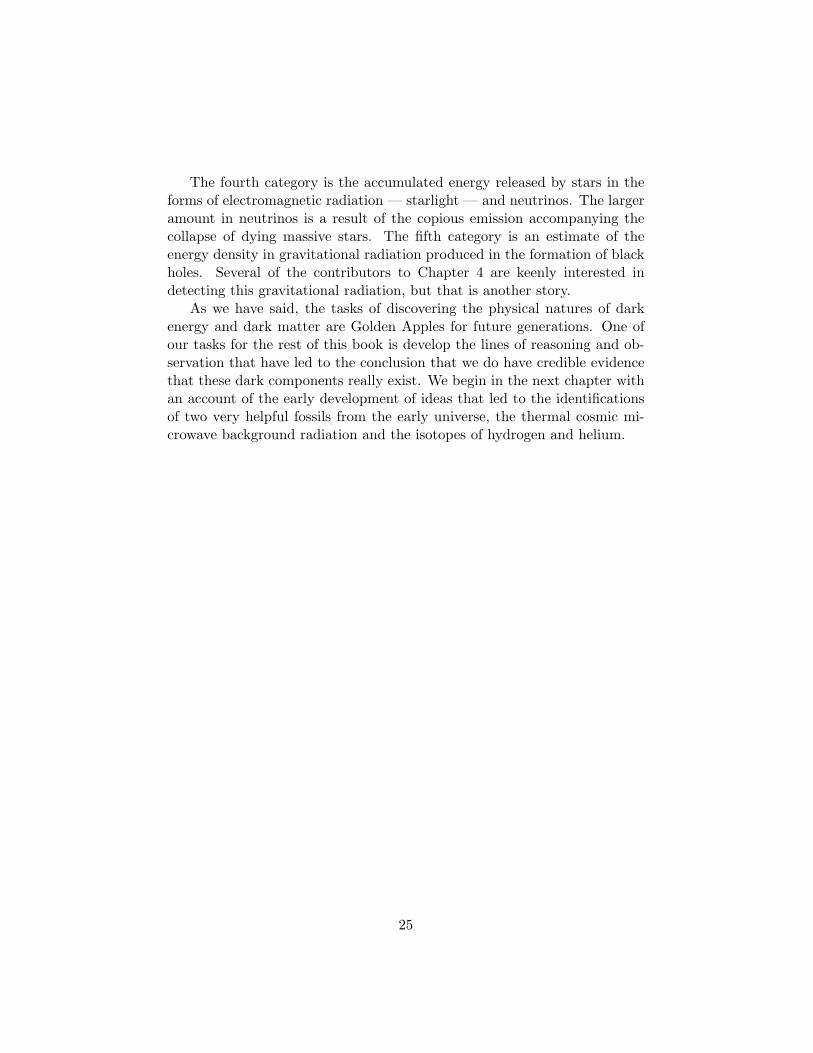
The details of the argument relating the abundance of helium to the tem-perature of the CMBR have since been refined, as will be described. But theAlpher and Herman consideration remains part of the standard cosmology.

Gamow recognized that the thermal radiation would not only be presentbut would remain an important dynamical actor after the early episodeof element formation. (For example, the paper Gamow 1948a presents anestimate of the time well after element formation when the mass densitiesin matter and radiation were equal and, as Gamow argued, the expandinguniverse became unstable to the gravitational growth of concentrations ofmatter.) Alpher and Herman (1948) clearly recognized that the thermalradiation would be present even now. Alpher and Herman (1950) went sofar as to convert the present temperature to the present mass density inradiation, producing the first estimate of the fifth line in Table 1. But theydid not recognize that the radiation might be detected by methods to bedescribed later in this chapter.

Yet another refinement of the theory of formation of the light elementsin a hot big bang is the process that fixes the relative number n/p of theneutrons and protons that enter the first step of element-building in equa-tion (6). In the paper Gamow (1948a) the value of n/p is left open: Gamowwas content to establish orders of magnitude. Hayashi (1950), on the otherhand, recognized that in this hot big bang cosmology n/p is determined byparticle physics reactions, as follows.

When the temperature in the early stages of expansion of the universewas above about 1010 K, and the universe had been expanding for less thana second, the radiation was hot enough to produce a thermal sea of electronsand their antiparticles, positrons, and a sea of neutrinos and antineutrinos(& and &), mainly by the reactions

% + % # e+ + e!, e+ + e! # & + &. (11)

These particles convert protons to neutrons and back again by the reactions

p + e! # n + &, n + e+ # p + &, n # p + e! + &. (12)

At temperatures above about 1010 K the reactions drive the ratio n/p ofnumbers of neutrons and protons to its thermal equilibrium value,

n/p = e!Q/kT , (13)

at temperature T .10 Here Q = (mn!mp)c2, where mn!mp is the di!erenceof mass of a neutron and of a proton, and k is the Boltzmann constant.

10In fact, n/p also depends on the lepton number, which is the sum of the numbers of e!

31

Hayashi found that as the universe expanded and cooled below 1010 Kthe reactions in equation (12) slowed to the point that the value of n/pfroze, and then n/p more slowly decreased as neutrons freely decayed toprotons (by the last reaction in eq. [12]) going to the right). By the timethe temperature had dropped to Tcrit the ratio of neutrons to protons hadfallen to about n/p $ 0.2. In the standard cosmology most of the neutronspresent at this time combined with protons to form deuterons, and mostof the deuterium burned to the heavy isotope of helium 4He, with a traceamount of 3He.

The paper Alpher, Follin and Herman (1953) presents a detailed applica-tion of Hayashi’s idea. Their analysis of how the ratio n/p of the numbers ofneutrons and protons varies as the universe expands and cools is essentiallythe modern computation. Enrico Fermi and Anthony Turkevich (in workthat is not published but is reported in Gamow 1949, ter Haar 1950, andin more detail in Alpher and Herman 1950, 1953) worked out the chains ofparticle exchange reactions that burn deuterium along with neutrons andprotons to helium and trace amounts of heavier elements. These analysescomplete the formulation of all the essential pieces of the established theoryof the origin of most of the isotopes of hydrogen and helium.

The hot big bang has become the standard model because it fits demand-ing tests. In the 1960s it was not at all obvious that that would happen,however, and people were discussing alternative ideas. They are part of thestory of how we arrived at a standard cosmology.

3.2. Nucleosynthesis in alternative cosmologies

The evidence developing in the 1950s was that the heavier elements wereproduced in stars. If so, might the stars also produce light elements? Ifthat were so helium production in a hot big bang could be a problem: itmight predict too much helium. But that can be fixed: one can adjust theprediction by adjusting the assumptions in the big bang model, or one cango to a steady state cosmology, for example. We review here some of thealternatives people were considereing. The point to notice is that these ideas

and # particles minus the numbers of e+ and #. The reactions in equations (11) and (12)do not change the lepton number: its value had to have been set by initial conditions veryearly in the expansion of the universe. Equation (13) assumes the absolute value of thelepton number density is small compared to the number density of CMBR photons. Apositive and large lepton number suppresses n/p, and a strongly negative lepton numberincreases n/p. This point figures in the cold big bang model discussed later in this section.The present observational constraints are consistent with the small lepton number assumedin equation (13).

32

arguably are as elegant as the standard hot big bang. We need observationsto show the way through the thickets of elegance. The following sectionstrace developments of the evidence.

Let us consider first what came of the idea that the heavy elements wereformed in the big bang along with the light elements. A problem with thisidea is that there is no stable atomic nucleus with mass 5 (that is, a totalof five neutrons plus protons). That means the abundant isotope of helium,with mass 4, cannot capture a neutron and then another one and subse-quently decay to an isotope of lithium by the emission of an electron. Thisstrongly suppresses the build-up of elements heavier than helium during therapid expansion of the early universe. Alpher (1948) remarks on the prob-lem, and a like situation at mass 8, in the published version of his doctoraldissertation. The analysis mentioned above by Enrico Fermi and AnthonyTurkevich failed to find a nuclear reaction that might carry significant nu-clear burning in the early universe past the mass-5 gap. But Gamow (1949)noted a possible way out that is worth considering here even though weknow now that it does not work.

Gamow’s (1949) idea was that if the mass density in baryons when thetemperature of the universe was Tcrit were much larger than previously con-sidered, and n/p were much smaller (as was later realized follows fromHayashi’s 1950 analysis of eq. [12]), then after all the neutrons had com-bined with protons to form heavier elements a substantial fraction of thebaryons would be left as protons, the nuclei of hydrogen atoms. That agreeswith what is observed. The larger matter density in the early universe wouldcause faster nuclear burning of deuterium, and perhaps push nuclear burningpast mass 5.

Hayashi and Nishida (1956) presented an analysis of this idea. Theyconsidered the possibility that the baryon number density at a given tem-perature is about a million times what is assumed in Gamow (1948a) andAlpher and Herman (1948). That lowers the present temperature of theCMBR by a large factor, which Hayashi and Nishida would not have countedas a problem because the CMBR was not known. They took account of thehelium-burning reactions

4He +4 He #8 Be + %, 8Be +4 He #12 C + %, (14)

which by then were known to be important in the evolution of stars after allthe hydrogen in the central regions had burned to helium. In this “cool” bigbang model universe, Hayashi and Nishida found significant production ofcarbon and oxygen. The deuterium abundance coming out of this model is

33

much too small, according to what is now known, and the helium abundanceis too large, though not by a large factor. (That is because almost all theneutrons that survive to the time when the temperature has fallen to Tcrit areburned to helium, and the value of n/p when deuterium starts accumulatingis not very sensitive to the density of matter.)

This cool big bang universe produces helium in an amount that might nothave seemed unreasonable at the time. It also produces a not insignificantamount of heavy elements. Layzer and Hively (1973) pointed out that theheavy elements produced in a cool big bang might form grains that wereable to absorb and reradiate starlight e!ectively enough to produce thethermal CMBR spectrum out of starlight. Here is an example of an ideathat is interesting but was not pursued, and, we now know, is not viable.The light element abundances are wrong, and it cannot account for therelation between the large-scale distributions of matter and the CMBR thatis discussed in Chapter 5.

Zel’dovich (1963, 1965) proposed a cold big bang cosmology, in whichelement production is left entirely to the stars. He was led to this by his inter-pretation of the observational evidence11 to mean that the background radi-ation temperature “does not exceed 1" K (Ohm 1961)” and that “the initialhelium content was below 10-20%.” Smirnov (1964, at At Zel’dovich’s sug-gestion, according to Smirnov’s acknowledgment) reanalyzed element pro-duction in a hot big bang. Smirnov showed that the small primeval heliumabundance could be accommodated in the hot big bang picture by lower-ing the matter density at a given radiation temperature, but that that thatwould imply an unacceptably large abundance of deuterium. (At Smirnov’slower density, neutrons and protons combine to form deuterium, but theburning of deuterium to helium is incomplete.) Zel’dovich (1965) notedanother apparent problem for the cool case: the radiation temperature atthe present matter density is unacceptably large. We now know that theCMBR temperature and helium abundance both are larger than Zel’dovichhad supposed, and they are consistent with each other within the hot bigbang. But Zel’dovich was led to propose an alternative.

In Zel’dovich’s cold model the very early universe contained equal num-ber densities of protons, electrons and neutrinos, all very nearly uniformlydistributed, and with energies that are as low as possible. This means one

11Osterbrock (page 63) describes what was known then about the helium abundance.The temperature estimate Zel’dovich mentioned was based on the Project Echo measure-ment discussed by Hogg, Novikov and others in chapter 4. Zel’dovich’s reaction to newsof the identification of the CMBR is described by Novikov (page 70) and is illustrated alsoby Zel’dovich’s letter to Dicke quoted on page 132.

34

has to consider the e!ect of the exclusion principle that limits the allowednumber densities of electrons and neutrinos at a given energy. The highdensity of electrons in the early universe would cause the electrons to fillall their available states up to a large energy. But the energetic electronscannot force themselves onto protons to make neutrons (by the first reac-tion going to the right in eq. [12]) because that requires the production ofneutrinos, and in this picture all the neutrino states with the energy allowedby the reaction are already taken.12 In this universe star formation wouldcommence with nearly pure hydrogen. This is yet another example of aninteresting universe that proves not to be the one we live in.

Hoyle and Tayler (1964) knew that the helium abundance is large, andgreater than seemed reasonable for production in stars. They too reconsid-ered the hot big bang model, but they also pointed to another possibility. Inthe steady state cosmology the universe always has been as it is now: therewould be no fossil helium. Hoyle and Tayler suggested that the helium couldhave been produced in the “little bangs” of very massive exploding stars.The local evolution of a very hot exploding star is similar to the evolution ofan expanding universe, and element formation is similar too. This is anotherinteresting universe that we now know is not ours. Like the cool big bang,it cannot account for the thermal CMBR and its spatial distribution.

Yet another alternative, that could eliminate fossil helium but not thefossil thermal radiation, was inspired by the following considerations. Ameasure of the relative strengths of the gravitational and electromagneticinteractions is the ratio of the gravitational and electric forces of attractionbetween an isolated electron and proton,

fgrav

fel=

Gmemp

e2$ 10!40. (15)

The charges of a proton and electron are ±e, and G is Newton’s gravita-tional constant. Since both forces vary in the same way with the separationof the particles (on laboratory scales) this ratio does not depend on the sep-aration. Its very small value led Dirac (1938) to ask whether the strengthof the gravitational interaction might be decreasing: maybe gravity is weaknow because the universes is old. Dicke liked Dirac’s proposal: to him it

12Another way to put this is that Zel’dovich assumed the lepton number mentionedin footnote 7 is positive and large enough to force the equilibrium ratio of neutrons toprotons at high density and low temperature to a value close to zero. Zel’dovich’s idea ofadjusting the cosmic lepton number can be extended to a hot big bang model; it changesthe relation between the helium abundance coming out of the big bang and the CMBRtemperature. The evidence now is that the lepton number is negligibly small.

35

fit the idea that local physics depends on the large-scale nature of the uni-verse. Perhaps gravity physics is determined by the large-scale distributionof matter, and the thinning of the mass as the universe expands decreasesthe strength of gravity. Dicke termed this idea Mach’s principle, after ErnstMach’s (1883) proposal that inertial motion is not absolute but rather isdetermined relative to the motion of matter at large. Dicke (1964) reviewsthese ideas. They inspired the proposal that general relativity be adjustedto a scalar-tensor gravity theory in which the number in equation (15) de-creases as the universe expands (Brans and Dicke 1961). Dirac’s argumentindependently led Pascual Jordan to the same theory and to his own con-siderations of the observational consequences (Jordan 1962).

Among the consequences of the Jordan-Brans-Dicke theory would be aconsiderable increase in the rate of expansion of the early universe relativeto general relativity. That would change the relation between the CMBRtemperature and the thermonuclear production of chemical elements in theearly universe. If the expansion were rapid enough there would be no particlereactions. This universe could have the observed present CMBR tempera-ture and baryon mass density and no light element formation outside stars.This is another idea that fascinates but failed. (Ideas tend to have long lives,however. The Jordan-Brans-Dicke theory, and the idea that numbers suchas the one in eq. [15] may vary with time, still figure in debates on earlyuniverse physics.)

3.3. Thermal radiation from a bouncing universe

The experiment that led to the recognition of the thermal cosmic microwavebackground radiation, and helped us sort out ideas about the nature of theearly universe, was inspired by a line of thought we have not yet mentioned:perhaps our expanding universe bounced from a previous state of collapse.As we will explain, the bounce might be expected to have filled space withthermal radiation — the CMBR.

Lemaıtre (1933) expressed the feeling that, from a purely aesthetic pointof view, a universe that successively expands and contracts to exceedinglysmall size has “un charme poetique incontestable et faisaient penser auphenix de la legende.” Wheeler (1958) asked whether the bounce in anoscillating universe might be compared to “a glove which is turning itselfinside out one finger at a time.” And Hoyle and Narlikar (1965) consideredthe idea that the universe is in a steady state overall, but that “pockets ofcreation” could set part of the universe into a local oscillation. That is, theconcept of bouncing universe certainly was not ignored. But the importantidea for our purpose is Tolman’s (1934) point that a bounce likely would

36

produce entropy, in the form of thermal radiation similar to what is nowknown to be present.

In the 1960s Robert Dicke (in an unpublished discussion that is de-scribed more completely in the essays) made Tolman’s argument more tan-gible. Dicke noted that the nuclear burning of four protons — the nuclei ofhydrogen atoms — into the nucleus of one helium atom in a star releasesenough energy to produce about one million starlight photons. The burningof helium to heavier elements produces still more starlight. These starlightphotons are shifted toward the red as the universe expands. If the expansioneventually stopped and the universe then collapsed back to high density thestarlight photons would then be shifted toward the blue, to greater energy.If the blueshift were large enough then just a few blueshifted starlight pho-tons would have enough energy to break apart each heavy atom, giving backthe protons. These protons would serve as fuel for nuclear burning in newgenerations of stars in the next cycle of expansion and collapse. The rest ofthe starlight photons would be thermalized, that is, turned into the CMBR.A few hundred bounces could make the observed energy density in thermalradiation out of starlight, if the bounces conserved the numbers of neutrons,protons and photons.

We now know that, according to general relativity theory, a collapsinguniverse does not bounce. But there are two reasons to highlight Dicke’sidea. First, we don’t know that general relativity theory provides a full andcomplete description of the very early stages of the expansion of the universe.More to the point of this book, Dicke’s line of thought was interesting enoughthat he was led to persuade two members of his Gravity Research Group,Peter Roll and David Wilkinson, to build an instrument capable of detectinga sea of thermal radiation. News of the Roll-Wilkinson experiment reachedArno Penzias and Robert Wilson, who had a detection of microwave emissionthey couldn’t interpret. How that happened is recalled in the essays in thenext chapter.

3.4. Detecting the cosmic microwave background radiation

We turn now to the observational and experimental work that led to thedetection and eventual interpretation of the cosmic microwave backgroundradiation.

A direct measurement of the intensity — or the equivalent (Rayleigh-Jeans) temperature — of a cosmic sea of photons employs a detector thatmeasures the flux of incident radiation. From that one must subtract allthe contributions from local sources in the ground, the atmosphere and our

37

Milky Way galaxy. There is another indirect approach that employs “ther-mometers” in the form of interstellar molecules. Both methods producedtantalizing clues to the existence of the CMBR well before it was identified.We begin with a description of the “thermometers,” because they providedan actual measurement of the present temperature of the universe two dozenyears before the radiation was recognized in 1965.

The indirect method is based on a result from quantum physics. Theenergy of an isolated object such as an atom or molecule has discrete possiblevalues: there is a ground level with energy E0, a first excited level withenergy E1, a second level at E2, and so on. The energy levels of an objectas large as a person would be fantastically closely spaced if we were able totruly isolate someone, but it can’t be done: we are tightly coupled to ourenvironment. The quantization of energy, however, is clear and distinct onthe much smaller scale of atoms and molecules. In a dilute gas of moleculesbathed in blackbody radiation at temperature T , the ratio of numbers inthe first excited level and the ground level is given by the equation

n1/n0 = e!(E1!E0)/kT . (16)

This has the same form as equation (13) for the equilibrium ratio of numbersof neutrons to protons in the early universe, but here applied at much lowerenergies and temperatures and much later in the history of the expandinguniverse.

The ratio n1/n0 for a species of molecules in interstellar space can bemeasured by comparing the strength of absorption of light from a back-ground star by the molecules in the two energy levels. Starlight photonsmay be absorbed by a molecule in its ground level, with energy E0, leav-ing the molecule in some highly excited level, with energy E#. The pho-ton has to supply the energy di!erence, E# ! E0. From Planck’s conditionE = h& we see that this absorption produces an absorption line at frequency&a = (E#!E0)/h in the spectrum of light from the star. A starlight photonwith the lower frequency &b = (E#!E1)/h can be absorbed by molecules inthe first excited level, leaving the molecule at energy E#. This produces asecond absorption line at &b. The ratio of the amount of absorption at thetwo frequencies is a measure of n1/n0. Since the energy di!erence E1 ! E0

is known equation (16) gives us a temperature. We have a thermometer.There is the problem that the temperature measured by the ratio n1/n0

is determined not only by the temperature of electromagnetic radiationbathing the molecules, but also by collisions with interstellar particles. Themolecule cyanogen (CN, a carbon atom bound to a nitrogen atom) in inter-stellar matter has the useful property that it recovers quickly from collisions

38

with particles, and its energy levels are well spaced for the measurementof radiation temperatures near that of the CMBR. (The energy di!erenceE1 ! E0 for cyanogen corresponds to the microwave wavelength 2.6 mm.)CN thus provides a very convenient thermometer.

McKellar (1941) used equation (16) to translate observations of absorp-tion of starlight by interstellar CN molecules in the two lowest levels to thetemperature

T & 2.3 K. (17)

With hindsight, the inference we would draw is that interstellar CN moleculesare bathed in the radiation field having this temperature. But the measure-ment was not so interpreted in the 1940s by either McKellar or by Adams(1941), who made the measurements. Herzberg (1950) comments that thistemperature “has of course a very restricted meaning.” The restriction hehad in mind likely is that, as we have noted, the excited levels of CN mightbe populated by particle collisions rather than radiation. Some astronomersknew that that would require a curiously high particle collision rate, how-ever, as will be discussed (page 59).

Astronomers are accustomed to dealing with complex situations thatrequire them to remember many curious things. In the 1960s some remem-bered McKellar’s temperature and recognized the possible relation to thehot big bang cosmology. How that happened is one of the threads runningthrough the essays.

The direct detection of the CMBR requires a receiver operating at somefrequency and an antenna to define the beam, that is, the range of directionsin the sky from which the radiation is received. The amount of radiationdetected must be corrected for the radiation that originates in the receiverand the thermal radiation emitted by our warm immediate surroundings, in-cluding the atmosphere. Two approaches to the unwanted “noise” radiationoriginating in the receiver figure in our story. One used low noise receiversdeveloped at the Bell Telephone Laboratories for the purpose of communi-cation. The other used a technique pioneered by Dicke: rapidly switch thereceiver between the sky and a reference “load” that is producing thermalradiation at a known temperature. The di!erence subtracts the radiationoriginating in the detector. The time average beats down the noise in the dif-ference signal. That leaves a measurement of the di!erence Ts! Tl betweenthe wanted sky temperature Ts and the known load temperature Tl. Dickeinvented this radiometer in the 1940s as part of war research at the Radi-ation Laboratory at the Massachusetts Institute of Technology. An earlyapplication was the measurement of the absorption of microwave radiation

39

by the atmosphere, which limited the push to radar at shorter wavelengthwhich would have provided better resolution. (Since microwave emissionfrom the atmosphere will become important later in our story, it is worthremarking here that if material at a nonzero temperature absorbs radia-tion then it also emits radiation. Wilkinson [page 139] emphasizes anotherpoint to bear in mind: the standard technique used by radio astronomersto measure the radiation received from an object is to compare the energyflux received when the detector beam is on the source and when the beamis directed to a point in the sky slightly o! the source. The subtractioneliminates a lot of the noise from the sky, ground and detector. But it doesnot work for observations of the CMBR because this radiation is uniformlydistributed across the sky.)

The essays describe how the CMBR was detected in measurements inNew Jersey that used the Bell Laboratories low noise receivers. Penzias andWilson found convincing evidence that this detection is real by using a coldreference load to establish a zero point for the measurements. The CMBRwas detected again a few months later in an independent experiment, also inNew Jersey and just 30 miles away, that used a Dicke microwave radiometer.This was the experiment by Roll and Wilkinson.

Figure 4 (from Lawson and Uhlenbeck 1950) is Dicke’s illustration of thesensitivity of his radiometer. In this example, the reference load was at roomtemperature and the switching was done by a wheel that swings the load intoand out of the waveguide connecting the detector and antenna. More recentmeasurements use electronic switching and loads with temperatures that arecolder and more closely matched to the CMBR. A Dicke radiometer “sees”thermal microwave radiation wherever the horn antenna is pointed, whetherat the ground, or people, or the atmosphere. The strip chart recording shownin Figure 4 indicates the change in response when the antenna was pointed atchimneys that were in use, and so slightly warmer than their surroundings.(Notice that the temperature scale is inverted: higher recorded temperaturesare indicated as lower positions in the chart.)

The top line in Figure 4, measured with the antenna scanning at an angleof 75" from the zenith, indicates a more or less uniform temperature of about125 K. Variations in the temperature from one part of the sky to the otherare small, less than about 10K. This means the instrument used at MITwas capable of detecting temperatures as small as 10K. Note also that thetemperature measured well away from hot chimneys increases as the anglefrom the zenith is increased from 75 to 90". Some of the increase in detectedtemperature at the larger zenith angle is the result of microwave emission bythe Earth’s atmosphere. When the instrument is aimed closer to the horizon,

40

Figure 4: An illustration of the ability of a Dicke radiometer to detect thermalradiation. Below is a sketch of the skyline of Cambridge in 1945, seen from the roofof a temporary building on the MIT campus. Above is a strip chart recording ofthe response of the radiometer to the warm chimneys. A higher temperature, as inthe direction of the building marked C, is recorded as a lower position on the chart.

it receives more atmospheric radiation because it is looking through a longerpath through the atmosphere.13 By measuring how the temperature varieswith the zenith angle, one can extrapolate to what would be detected in thelimit of no atmospheric emission. This would be the observed temperatureof space beyond the Earth’s atmosphere. We should add that some of theincrease in measured temperature shown in Figure 4 results from what radioastronomers call “side-lobe pickup.” A radio frequency antenna does notproduce a sharply defined beam on the sky. Rather, there are subsidiarydi!raction maxima, known as side lobes, that allow radiation to leak into thereceiver from substantial angles away from the optical axis. As the zenithangle increases, these side lobes pick up more and more radiation from the

13In the approximation of the atmosphere as a plain-parallel slab of emitting materialthe detected atmospheric emission varies with the secant of the zenith angle.

41

Figure 5: A tipping measurement (Ohm 1961). The top curve shows the sum ofthe microwave radiation flux from the detector, ground, atmosphere, and whatevercomes in from above the atmosphere. The lower curve is the result of subtractingestimates of what came from the instrument and ground.

$ 300 K ground. Side lobe pickup bedeviled early attempts to measure bothatmospheric emission and the CMBR spectrum.

Dicke, Beringer, Kyhl and Vane (1946) used a “tipping experiment” toestablish that “there is very little (< 20"K) radiation from cosmic matter”at the microwave wavelength ($ 1 cm) they employed. Ironically, this paperappears in the same volume of the Physical Review as Gamow’s 1946 letteron nucleosynthesis. Gamow was not yet discussing a hot big bang, however,so it is not surprising that neither paper made reference to the possiblesignificance of the other. The bound Dicke and colleagues placed on howhot space might be is well above what would be expected in the cool bigbang situation Hayashi and Nishida (1956) later analysed. It is not far fromthe situation Gamow (1948a) had proposed and Alpher and Herman (1948)calculated, however, and it is close to what we now know is the temperatureof the fossil radiation from the big bang, T0 = 2.725 K. But the connectionbetween what Dicke’s radiometer can measure and what might be expectedfrom a hot big bang was not noticed for another two decades.

In the course of research on other subjects in the 1950s and early 1960smeasurements equivalent to the Dicke et al. tipping experiment were re-peated with better sensitivity, and the CMBR detected. Eventually theradiation was recognized. That happened first as a byproduct of research

42

at Bell Telephone Laboratories to develop low noise maser amplifiers forreceiving systems for communication (DeGrasse, Hogg, Ohm and Scoville1959; Ohm 1961; Jakes 1963).

Figure 5 shows a particularly detailed tipping measurement from thiscommunications program. These data are from Project Echo, which demon-strated communication by microwave signals sent from the ground and re-flected back to the ground by a satellite (a large balloon with a conductingsurface). The paper Ohm (1961) presents the following numbers. Whenthe Echo receiver was pointed to the zenith it detected microwave radiationequivalent to blackbody radiation at temperature Tsystem = 22.2 ± 2.2 K at2390 MHz (12.6 cm wavelength). When the instrument was tipped awayfrom the zenith the system temperature increased because it was lookingthrough more atmosphere. From that variation one could estimate thatthe atmosphere contributed the equivalent of Tatm = 2.3± 0.2 K. That plusestimates of the radiation originating in the instrument and the radiation en-tering the horn antenna from the ground was, in this experiment, estimatedto total Tlocal = 18.9 ± 3.0 K. The di!erence,

Texcess = Tsystem ! Tlocal = 3.3 ± 3.7 K, (18)

is a measure of what might be entering the atmosphere from cosmic sources.This is a considerable improvement over the Dicke, Beringer, Kyhl and Vane(1946) bound, Texcess < 20 K. The central value in equation (18) is consis-tent with the Alpher and Herman (1948) estimate of the Gamow condition(eq. [9]), within the uncertainties, and it is close to what we now know isthe CMBR temperature (eq. [10]). The stated uncertainty in Tlocal on equa-tion (18) is conservative because the errors were added in absolute value,but even if added in quadrature Texcess is formally consistent with zero.

The measurement was repeated in the Telstar Project that demonstratedtransmission of a television signal from the ground to a satellite that rera-diated the signal back down to the ground. Jakes (1963) reports that (at7.3 cm wavelength) “The over-all system noise temperature was measuredto be somewhat less than 17"K pointing at the zenith, which included about4.5"K for waveguide losses, 2.5"K sky noise, 2.5"K for antenna side lobesand heat losses and 5"K for the maser.” The sum and di!erence — whichJakes does not state — amounts to

Texcess = Tsystem ! Tlocal = 2.5 K. (19)

This is close to the central value of Texcess from Project Echo, and againclose to what is now known to be the CMBR temperature.

43

The consistency of central values of Texcess from the Echo and Telstar sys-tems did not force attention to the idea that there might be a detectable seaof extraterrestrial microwave radiation: a reader of these papers could imag-ine that local sources of radiation had been underestimated. That might bewhat Ohm (1961) had in mind in writing that ‘the “+” temperature pos-sibilities of Table II [listing local noise contributions] must predominate.’We know in hindsight that there is no need to assume the system tempera-tures in the Echo and Telstar systems were systematically underestimated;the contribution of radiation entering the horn antenna from the groundactually is an overestimate. All this became clear later in the 1960s whenPenzias and Wilson added a low temperature calibrator to the Telstar sys-tem, for purposes they explain in Chapter 4. That made the di!erenceTexcess between what was detected and what was expected from the instru-ment, ground and atmosphere a clear and pressing issue for them, and itsoon became a pressing issue for the cosmology community.

Let us consider next how the reaction of the community was conditionedby the state of research in cosmology in the early 1960s.

3.5. Cosmology in 1960

In our experience the book Cosmology by Herman Bondi (in two editions,Bondi 1952 and Bondi 1960a) gives a good picture of research in this subjectin the 1950s and early 1960s. Bondi reported the vigorous debate on therelative merits of the steady state and relativistic big bang cosmologies, andhe assessed the state of observational tests of these and the other cosmologiesthen under discussion. And he showed us a vivid picture of the role of thephilosophies that implicitly or explicitly inform our approaches to the theoryand the observations.

Bondi also surveyed a broad range of issues about the fundamental basisfor physical cosmology. Is the universe really close to homogeneous in thelarge-scale average? Are the redshifts of the galaxies really due to the expan-sion of the universe, as opposed to a “tired light” e!ect? Perhaps light tendsto shift toward longer wavelength as it moves across the immense distancesbetween the galaxies (Zwicky 1929). If the redshift is an e!ect of expan-sion how do we know the universe is evolving, as opposed to the idea thatcontinual creation of matter is keeping it in a steady state? If the evidencewere that the universe is evolving how would we know that the evolution iswell described by general relativity theory? In an evolving universe wouldthe laws of microscopic physics really be the same now and in the remotepast when the universe is supposed to have been so very di!erent? If therelativistic cosmological model were a good approximation what would be

44

reasonable values for its parameters? Must we imagine that an evolvinguniverse expanded from a formal singular state of arbitrarily high density,or might we suppose that we observe expansion now following a bounce thatterminated an earlier collapsing state? If our universe is evolving how mightit end, in a big freeze or a big crunch?14 And does it make sense to allowthe possible role for Einstein’s cosmological constant that is illustrated inFigure 1 on page 13?

This is a disconcertingly long list of questions, but it does not meanthat the cosmology Bondi described was an empty science. People wereassembling observational evidence, in part out of simple curiosity, in partdriven by the goal of testing theoretical ideas, and the observations were inturn driving theoretical developments.

Sandage’s (1961) pioneering paper, The Ability of the 200-inch Telescopeto Discriminate Between Selected World Models, explored the feasibility oftesting cosmological models, and perhaps distinguishing between the steadystate and big bang models, from the observations of galaxies at low andhigh redshift. The steady state cosmology has the distinct advantage forobservers that it makes definite predictions: the galaxy populations at greatdistances, seen as they were in the past because of the light travel time,are supposed to be statistically the same as what is observed nearby. Thismeans the counts and apparent magnitudes (brightness in the sky) of thegalaxies are predicted functions of their redshifts. The big bang modelhas free parameters — space curvature and # — and it predicts that thegalaxies observed at great distances are younger and statistically di!erentfrom what we see nearby (though the expected degree of di!erence still isdi"cult to predict). The theoretical basis for the tests Sandage consideredwas understood in the 1930s. The new development in the early 1960s wasthe availability of the large collecting area of the 200-inch Hale telescope.

Sandage (1961) concluded that with the technology at hand the best wayto distinguish between the steady state model and the family of big bangmodels was the relation between redshifts and absolute magnitudes of themost luminous galaxies, which seem to have close to the same luminosities.He presented an application of the redshift-magnitude test for observationsthat reach galaxies at redshift z = 0.46, meaning the universe has expandedby the factor 1.46 since the light we receive left the galaxy (as expressedin eq. [2]). This is an impressively deep probe out in space and back intime. But he concluded that, even with the power of the 200-inch telescope,distinguishing between the steady state and big bang models will be “di"cult

14Bondi (1952, 1960a) avoids these terms, along with big bang.

45

and perhaps marginal.”15

Another suite of issues, that generated considerable research activity inthe early 1960s, concerned the ages of the stars, from the theory of stellarevolution, and the age of the elements, from the decay of long-lived radioac-tive isotopes. There was debate on three aspects of these time scales. First,in the standard big bang model the universe has expanded from densitiesand temperatures too large for stars to have existed. That means that inthis cosmology the oldest stars are younger than the cosmic expansion time.Sandage (1961) concluded that the big bang cosmology can satisfy this con-straint, but that it might require the postulate of a positive cosmologicalconstant. Second, in the big bang model the epoch of galaxy formationmight have ended by now, but in the steady state picture we expect to seearound us a mix of young and old galaxies from the contimual creation ofmatter. There are apparently young galaxies nearby. Hoyle and Narlikar(1962) took that as an argument for the steady state picture. Gamow (1954),on the other hand, made the now generally accepted point that the colorsof most nearby galaxies do not scatter much, consistent with a close touniform age of most of the stars, and inconsistent with the steady statepicture. Third, galaxies observed at great distance are seen as they were inthe past, because of the time required for the light to reach us. Thus in theBig Bang cosmology galaxies observed at high redshifts would be expectedto appear younger than nearby ones, while in the steady state cosmologythe mix of young and old galaxies was the same in the past as it is now.That led Bondi (1960b) to state that if distant galaxies were observed to besystematically di!erent from those observed nearby then “the steady-statetheory is stone dead.” In the early 1960s there was no credible evidence fora systematic di!erence between galaxies at low redshift and high. This wasa good argument that was not widely acknowledged.16

15Modern applications of this redshift-magnitude test use the light from supernovaerather than galaxies, and reach expansion factors 1+ z close to 3. The apparently modestbut deeply important increase in the distances the observations reach indicates that theredshift-magnitude relation is close to the steady state prediction. The task of explainingwhy this is now taken as evidence for the e!ect of the cosmological constant " illustratedin Figure 1, rather than as evidence for the steady state cosmology, is left to Chapter 5,which addresses the current and accepted answers to the list of questions in the secondparagraph of this section.

16The situation began to change in the mid 1960s with the discovery of quasars, whichare considerable more abundant at redshifts z > 0.5 than nearby. The interpretationproposed then, and now well checked, is that quasars were more abundant in the past(Longair 1966; Sciama and Rees 1966). The use of Hubble’s law (eq. [1]) to convertquasar redshifts to distances certainly could be questioned (Terrell 1964; Hoyle 1965;Hoyle and Burbidge 1966). But that has since been checked by the demonstration that

46

Another issue under discussion in the early 1960s was the origin of thechemical elements. In the steady state cosmology matter is continually cre-ated. Bondi opined that creation of matter with the observed relative abun-dances of the chemical elements and their isotopes would be bizarre. Thatled him to conclude that a demonstration that the elements could not beproduced — presumably in stars — in the universe as it is now would bestrong evidence against the steady state cosmology, while a demonstrationthat the elements did come from stars would reduce the list of argumentsfor a big bang. Bondi (1952), in his first edition, had references to workon the theory of element formation in stars and in a hot big bang, but thediscussion was brief. By the time of the second edition, Bondi (1960a) couldreport significant advances in the theory of element formation in stars (Bur-bidge, Burbidge, Fowler and Hoyle 1957; Cameron 1957). This importantdevelopment was encouraging for the steady state philosophy. As Gamow(1956) noted, however, it was not necessarily a challenge for the big bangpicture: one could image nuclear reactions in stars somewhat altered whatcame out of the big bang. But the abundance of helium o!ered a criticaltest.

Burbidge (1958) recognized that the helium abundance in the MilkyWay is larger than might be expected from production in known types ofstars in the numbers indicated by the stellar luminosity of the galaxy. Hepointed out that some other galaxies are very luminous in radio emission,and that the energy released by conversion of hydrogen to helium mightpower these sources. He did not mention the possibility of helium productionin a big bang. Gamow (1956) did: “the calculations in that direction, carriedout by the present writer,” (Gamow 1948) “and later in some more detailby Fermi and Turkevich,” “lead to a value of the H/He ratio which is ingood agreement with observational data.” Gamow did not document theobservational evidence he mentioned. In the second edition of his book,Cosmology, Bondi (1960a, p. 58) added this assessment of the situation:

Since it has also been shown that any hot dense early state of theuniverse could not have left us any nuclei heavier than helium,the origin of such nuclei is no longer a question of cosmology.

when a quasar appears in the sky close to a galaxy at lower redshift the gas in the galaxyproduces absorption lines in the quasar spectrum. The quasar clearly is behind the galaxy,as the conventional interpretation of its redshift indicates. Modern observations also showthat more distant galaxies indeed appear distinctly younger, containing larger numbersof massive short-lived stars. And while the data on ages are much improved from whatSandage had in 1961, they still seem to require the postulate of a cosmological constant(or something that acts like one).

47

It might however be said that the abundance of helium mayconceivably be greater than would be accounted for by ordinarystellar transmutation and so might have to be explained on acosmological basis, but the evidence as yet is far too slight tomerit serious consideration now.

Bondi did not give references to the measurements of helium abundances.The big bang theory for helium formation is not mentioned in the text either,but there is a reference in the bibliography, to Alpher and Herman (1950).

Osterbrock and Rogerson (1961) presented measurements of the abun-dances of helium and heavier elements in the plasma around and betweenthe stars and in the Sun. They concluded that the mass fraction, Y , in he-lium is considerably larger than the mass fraction in heavier elements, andthat Y is not much di!erent in the Sun from what is observed in the presentinterstellar plasma. At the time it was known that asteroids are about 5billion years old (from radioactive decay ages; e.g. Patterson 1955). Thisis a reasonable estimate for the age of the Solar System. Osterbrock andRogerson concluded

It is of course quite conceivable that the helium abundance of inter-stellar matter has not changed appreciably in the past 5 % 109 years,if the stars in which helium was produced did not return much of itto space, and if the original helium abundance was high. The heliumabundance Y = 0.32 existing since such an early epoch could be atleast in part the original abundance of helium from the time the uni-verse formed, for the build-up of elements to helium can be understoodwithout di"culty on the explosive formation picture.

Their reference is to Gamow (1949).We believe that in this paper Osterbrock and Rogerson presented the first

well-documented proposal of a relation between the theory and observationalevidence of the presence of a fossil from the early universe. It appeared inPublications of the Astronomical Society of the Pacific, a journal that was(and is) familiar to astronomers and even to some physicists. But we havefound no evidence that anyone recognized the significance of this paper forcosmology before the mid 1960s, when the evidence for detection of theCMBR was recognized.

It is worth noting several papers in the early 1960s that referred to Os-terbrock and Rogerson (1961), and some that did not. Peebles (1964) usedtheir helium abundance in a study of the structure of the planet Jupiter,but did not notice the big bang connection. This discussed on page 127.

48

O’dell, Peimbert and Kinman (1964) added to the evidence for a large he-lium abundance in old stars, and reemphasized Burbidge’s (1958) point thatthe production of this amount of helium in an early generation of stars wouldrequire that the galaxy passed through an exceedingly luminous phase. Theyreferred to Osterbrock and Rogerson’s paper but did not mention the pos-sibility of helium production in a big bang. We have noted the reanalysesof the theory of light element production in big bang by Smirnov (1964)and Hoyle and Tayler (1964). Smirnov did not know the Osterbrock andRogerson paper: he thought the abundance of helium in the oldest stars isless than about 10%. Hoyle and Tayler knew the evidence that the heliumabundance is larger than that, and that the big bang model could accountit, but their do not include Osterbrock and Rogerson (1961).

The idea of another fossil, a remnant thermal sea of radiation that mightbe expected to accompany the production of helium in a hot big bang, wasclearly stated by Alpher and Herman (1948, 1950).17 The idea was notvery visible in the early 1960s, however, as is illustrated by the fact thatBondi (1952, 1960a) did not mention the radiation. Alpher and Herman(2001) recall asking radio astronomers about the possibility of detectingthe radiation, Tayler (1990), in his recollections of the work with Hoylein 1964 on helium production, mentioned their thoughts about remnantradiation from a big bang, and Hoyle (1981) recalls discussions of the possibletemperature of a microwave background in conversations with Gamow andwith Dicke. It seems clear that the idea that space might be filled witha sea of thermal radiation left from the early stages of expansion of theuniverse was “in the air” in the early 1960s. But it was not very visible inthe literature.

There were early measurements that constrained the possible temper-ature of this radiation. We noted in section 4 of this chapter that Dicke,Beringer, Kyhl and Vane (1946) had placed a limit T0 < 20 K on the e!ec-tive temperature of background radiation at microwave wavelengths. Theymade no mention of cosmology. The same is true of Medd and Covington(1958), who found that the sky temperature (the radiation from the atmo-sphere plus what we now know to be the CMBR) at 10.7 cm wavelength is5.5K, with a probable error of about 6 K, of Denisse, Lequeux and Le Roux(1957), who placed a limit of about 3 K on the background temperature at

17The idea was less clearly expressed by Gamow (1948); he did note that the radiationwould be present after element formation, and that it could be an important dynamicalactor in structure formation. This is discussed on page 51. Gamow (1956) arrived at apresent temperature of about 6K, but from a mistaken computation of cosmic expansiontimes, not from his earlier and now accepted considerations of helium production.

49

33 cm wavelength,18 and of Shmaonov (1957), who found about 4± 3 K at3.2 cm. Within the uncertainties of the measurements, these all are upperbounds, not unrecognized detections.

With the clarity of hindsight we conclude that the Bell Laboratoriesmeasurements (DeGrasse et al. 1959a, Ohm 1961) that were discussed com-mencing on page 43) were the first likely — though not recognized — de-tection of the CMBR to be presented in the literature, and that McKellar(1941) presented the first analysis of a likely indirect detection from inter-stellar absorption lines. Hindsight is needed, of course, because until theevents in 1965 described in the next chapter no one had recognized the pos-sible significance of these measurements. Doroshkevich and Novikov (1964)likely were the first to recognize the importance of the Bell Laboratoriesmeasurements for cosmology. Doroshkevich and Novikov might be countedas the second authors, after Osterbrock and Rogerson (1961), to make aconnection between measurements and a theory of a candidate fossil fromthe early universe. (The connection in this case was somewhat less com-plete, however, because Doroshkevich and Novikov did not realize that theBell Laboratories had a likely detection).

The recollections in the next chapter make it clear that some astronomersin the early 1960s remembered the evidence we have reviewed (commencingon page 38) that the spin excitation temperature of the interstellar moleculecyanogen is surprisingly large, and that that suggested the presence of amicrowave radiation background at an e!ective temperature of a few degreesabove absolute zero. But only after the candidate fossil radiation had beenrecognized in direct detection was it realized that the spin temperature is

18Lequeux, one of the authors of this last paper, o!ers this comment on the suggestionby Le Floch and Bretenaker (1991) that this experiment may have yielded a detectionrather than a limit: “In the winter of 1954-55, we measured the antenna pattern of aformer German ”Wurzburg” radar equiped with a 33-cm receiver built by Le Roux, thatwe used for mapping the Galaxy. This involved measuring the signal received from aremote transmitter while pointing the antenna in various directions. Then we calculatedthe contribution of the ground and the atmosphere to the antenna temperature as afunction of the direction pointed by the antenna, and compared to observation (far fromthe galactic plane, of course). The observed antenna temperature was calibrated withblackbodies. Then we concluded that any contribution from the sky would be less than3K, and would be rather uniform. This is what is published in the Comptes Rendus; andsigned by Le Roux.

“Given our equipment, and in spite of careful measurements, it would have been foolishto claim a positive detection. Our remote antenna lobes were considerably stronger thanthose of the horn used by Penzias and Wilson. Thus in the Comptes Rendus paper weonly claim an upper for the CMBR, admittedly close to the actual value, but only anupper limit.”

50

about what is wanted to account for the abundance of helium.There was one other – very indirect – hint to fossils from the big bang,

from large-scale structure: galaxies and clusters of galaxies. Bondi (1960a,p. 176) gave references to studies developing the idea that the present-day concentrations of mass observed in galaxies and in clusters of galaxiesgrew by gravity out of small departures from an exactly homogeneous massdistribution in the early universe. However, he does not take note of twoof Gamow’s (1948a,b) remarks that have proved to be part of our presentstandard model. First, the CMBR temperature set the matter temperaturein the early universe (because at high redshift the matter was ionized andthermally coupled to the radiation), and the matter temperature set theminimum mass of a cloud of matter that gravity can hold together againstthe matter pressure. Second, the gravitational growth of nonrelativisticmass concentrations such as galaxies commenced when the mass densityin the CMBR fell below the mass density in matter. Prior to that, therapid expansion driven by the large mass density in radiation suppressedthe gravitational growth of concentrations of matter. Gamow’s two pointswere little noted at the time we are considering: the only reference we havefound in the literature, apart from his immediate colleagues, is by ter Haar(1950, p. 129). The essays indicate how the role of the CMBR in theformation of galaxies and clusters of galaxies came to the general attentionof the community.19

A central theme of this chapter is that we find our way through elegantideas to the ones that actually approximate reality by an iterative consul-tation of theory and practice. The process tends to be haphazard. Most ofthe pieces needed to identify two fossils from the early universe — heliumand the CMBR — were known in 1960, but no one person knew enoughof them then to put them all together. Many have wondered why this laststep took so long. The essays in the next chapter o!er the best hope for anunderstanding of the answer.

19A related issue is the e!ect of the growing concentrations of mass on the spatial andangular distribution of the CMBR. The basic principles were developed in the 1960s afterthe identification of the CMBR (Sachs and Wolfe 1967; Silk 1967; Peebles and Yu 1970).Detection of the e!ect took some two more decades of work. The learning curve for howto make these measurements is a central topic of Chapter 5. The precision results arecentral to the network of cosmological tests that confirm basic elements of the presentstandard general relativity hot big bang cosmological model.

51

Chapter 4. Cosmology in the 1960s

Here are the essays, preceded by these few cautionary remarks.The plan of ordering of the essays is to group by topic, with chronolog-

ical order within groups and of the groups. Because the focus of researchtends to evolve with time the result is that these recollections of what hap-pened are presented in a roughly chronological order. For example, in thesecond half of the 1960s a first order of business on the experimental sidewas the measurement of the spectrum of the CMBR, and on the theoreti-cal side it was the exploration of ideas about what a significant departurefrom a thermal spectrum might mean. These continued to be pressing issuesin the 1970s, but there was increasing interest in the search for departuresfrom an exactly isotropic distribution of the radiation and for the theory ofthe disturbances to the CMBR distribution that might be expected to ac-company the known departures from an exactly homogeneous and isotropicdistribution of the matter. Thus we present the essays whose main focusis the spectrum before those largely concerned with the anisotropy of theCMBR.

In practice this plan requires many arbitrary and debatable decisions ontopics and dates. The result, we have checked by observation, is that it isnot readily apparent that we had a plan. This is a realistic illustration ofwhat was happening in the 1960s, of course.

The confusion extends to the recollections: they are not always evenconsistent with each other. The reader therefore must be prepared for adistinct change of style from the linear — but we hope e"cient — historyin the previous chapter to the chaos of the real world.

52

David C. Hogg: Early Low-Noise and Related Studies at BellLaboratories, Holmdel, N.J.

The US National Academy of Engineering cites Hogg’s election to the Academyfor his “contributions to the understanding of electromagnetic propagation atmicrowave frequencies through the atmosphere.” A native of Saskatchewan,Hogg’s current interest is the composition of music.

A giant in radio science, Harald T. Friis (1971) was head of the Bell radio-research laboratory in Holmdel. Having pioneered work on the superhetero-dyne receiver in the late 1920s, he played a key role in Karl Jansky’s ini-tial experiments and the beginning of radio astronomy in the early 1930s.His interests then turned to shorter wavelengths which eventually led to theconstruction of a nationwide microwave radio-relay system employing “horn-reflector” antennas that he patented with Al Beck. This design of antennais highly e"cient and was used in all of the low-noise microwave systemsto be discussed here. These remarks are made to indicate that high-qualityequipment, designed for very practical purposes, can be used as a tool forfirst-class science. It is to the credit of the United States that the ATT BellLaboratories existed, allowing such broadminded interactive research to bedone.

In the 1950s, not long after John R. Pierce had traveled to the U.K., in-cluding Oxford, he brought Rudi Kompfner to Bell Labs. They asked me tocalculate the thermal noise from the earth’s atmosphere over the microwaveband. This noise level was needed for their calculation of the feasibility ofmicrowave communication by reflection from an orbiting balloon (Pierce &Kompfner 1959). It was fortunate that some time earlier, with Arthur B.Crawford, I had measured the millimeter-wave absorption by the oxygenand water vapor in the sea-level atmosphere (Crawford & Hogg 1956). Thusthe broadening constants for computation of “sky noise” were determinedand that calculation was completed (Hogg 1959).

However, no sky noise measurements were available to corroborate thistheory. Nevertheless, again fortunately, at that time Derek Scovil and BobDe Grasse at the Bell Laboratory, Murray Hill, N. J., were well along indeveloping microwave traveling-wave (TWM) solid-state masers, with noisetemperatures on the order 10 K (De Grasse, Shulz-Du-Bois & Scovil 1959).Again encouraged by Kompfner and Pierce, we therefore combined thismaser and antenna to produce a “low-noise” receiving system.

Here we discuss and compare several systems at various microwave fre-quencies, with emphasis on the technology and low-noise results that pointedthe way toward a determination of the microwave cosmic background noise.

53

Figure 6: The antenna in the firstlow-noise microwave system

Figure 7: Horn-reflector antenna used inthe Project Echo experiment

In all three cases, the equipment was designed and built to demonstrate thefeasibility of satellite communications, and the cooperation of NASA andthe Bell Laboratories System Department were important factors.

The first low-noise microwave system (De Grasse, Hogg, Ohm & Scovil1959a,b) operated at 5.65 GHz. The antenna mount, constructed of wood,on the lip of Crawford Hill, allowed manual beam pointing in elevation only;a photograph is shown in Figure 6. The rectangular waveguide input tothe TWM was fed via a rotating joint in the circular waveguide from theantenna. The output from the TWM preamplifier was then fed to a con-ventional superheterodyne. This combination resulted in a (zenith) systemnoise temperature of 18.5 K.

At that time I was invited by John Shakeshaft to Cambridge, England,and gave these results in Maxwell’s lecture room at the Old Cavendish. Aseminar also was given at the old McDonald physics building at McGillUniversity, Montreal, Canada, where Ernest Rutherford did research on thealpha particle and helium.

Although this system was unsophisticated, it did serve as a prototypefor the following two systems that were used for actual communications viasatellites: Echo and Telstar.

The second low-noise microwave system (Ohm 1961) was designed andbuilt specifically for the Echo satellite project at a frequency of 2.39 GHz, forreceiving signals reflected from an orbiting balloon. The receiver design wasengineered by Ed A. Ohm and the project engineer was W.C. (Bill) JakesJr. The antenna (Crawford, Hogg & Hunt 1961), a twenty-foot aperturehorn-reflector, is shown in Figure 7; design and construction was managedprimarily by Arthur B. Crawford and Henry W. Anderson. The 2.39-GHzmeasured radiation patterns and gains were found to agree well with theory

54

(Crawford, Hogg & Hunt 1961); both azimuth and elevation pointing wereavailable. The dual-channel TWM, provided by the Derek Scovil group atthe Murray Hill Laboratory, received waves of both clockwise and counter-clockwise circular polarization, with a noise temperature of 7 K. Ohm carriedout an exhaustive study of the uncertainties in the measured and estimatednoise contributions. The overall system noise temperature (at zenith) was21 K.

The third low-noise system operated at 4.17 GHz as a sensitive receiverfor the Crawford Hill station of the Telstar Project (Jakes 1963). The an-tenna was the same as for the 2.39 GHz Echo experiment (Fig. 7), but gain,beamwidths, and pointing characteristics were checked at the new shorterwavelength and found satisfactory when compared with theory. The TWM,with a 5K noise temperature, was provided by the Scovil group to amplifyboth senses of circular polarization.

The “first-ever” live TV from Europe was obtained via Telstar with thisreceiver. The overall zenith system noise temperature was just less than17 K. W. C. Jakes Jr. was project engineer. The main U.S. ground stationwas at Andover, Maine.

Table 1. Summary of Satellite Communication Systems

Experimental Communication System 1 2 3

Frequency 5.65 2.39 4.17Estimated antenna backlobe and resistive noise 3.5 2.3 2.5Zenith atmospheric noise measured 2.5 2.3 2.5

estimated 2.75 2.4 2.5Zenith system noise measured 18.5 21 17

estimated 18.5 19 14.5

Note. — noise temperatures are in degrees Kelvin, frequencies in GHz

Table 1 shows that the zenith atmospheric sky noise, measured by tippingthe antenna beam in elevation, is within 0.25 K of the theoretical computa-tion in the microwave band; the theoretical values are computed for averagesummer conditions of temperature and humidity (U.S.A).

The table also shows that in no case does the estimated system tem-perature exceed the measured system temperature. Of course, none of theestimated system temperatures contain any contribution from the cosmicbackground radiation. However, it is amusing that, in the case of system 1,the estimated is the same as measured; this indicates sizable uncertainties,probably in both quantities.

55

Many of the uncertainties in the noise contributions from the microwavecircuitry can be avoided by switching between the antenna and a preciselycalibrated cold load located near the antenna input per se as shown by Pen-zias and Wilson (1965), at 4.08 GHz. With this improved measuring systemthey were able to deduce 3.5 K excess to the expected antenna temperature;this excess is interpreted as the cosmic background radiation.

The very low-loss switch used in these measurements is a treasure inmicrowave radiometry. It is made of a gently squeezed section of waveguideof circular cross section. Penzias and Wilson quote only 0.027 dB of loss fortheir switch; to my knowledge, it was first mentioned by George C. South-worth in his book on microwave technology and was first used in radiometryby Douglas H. Ring at K-band.

However, measuring the contribution of the lower hemisphere (backlobes) to the antenna temperature is quite another matter (for some es-timated values, see Table 1). Ideally, one would measure the antenna radia-tion pattern over the lower hemisphere, measure the ground (etc.) radiationover that same hemisphere, and integrate the product of those two over thehemisphere. This radiation is comprised of both emission from the groundsurface and reflection of sky temperature by that surface (Hogg 1968). Pen-zias and Wilson calculated a net contribution of just less than 1 K for theantenna per se. Apparently further research on antenna design, measure-ments and siting is called for.

As implied in the historical introduction, some equipment, designed andbuilt for practical (economic) application, can impact scientific studies, pro-vided the quality is good. An example of this is the fruitful use of electro-magnetic and electronic equipments, designed for microwave satellite com-munications development, in pursuing the microwave cosmic backgroundradiation.

Recently, the importance of science and engineering innovation to theU.S.A. has been emphasized in a proclamation by the President of the U.S.,backed by a report issued by a panel supported by the National Academies,and chaired by Norman Augustine. That there is fruitful feedback betweenthe two is well exemplified by the exercise we have just discussed. Thecosmologists and astronomers who carry on such research and innovationare to be commended.

56

Neville J. Woolf: Conversations with Dicke

Nick Woolf is a professor of astronomy at the University of Arizona. He wasa postdoc in the Princeton University Department of Astrophysical Sciencesin 1962 – 65. His current research interest is astrobiology.

I have these memories that tell me that I cost Bob Dicke the Nobel Prize.One evening in the attic of Palmer, I think in early 1964, Bob turned

to me and asked me whether there was any way to know the amount of thebackground radiation. He had already turned Roll and Wilkinson onto thetopic, but I believe they had only just started.

I said “Well, there were your own measurements in 1946.” He grunted.And I said, “and then there are the interstellar molecules.”

He didn’t say a word. “Oh”, I thought, “I must have said somethingstupid” and I shut up. If I had said more, about the searches for excitationin Iron and CN and the other stu!, I am sure he would have picked up onit and he would have been ahead of Penzias and Wilson - but that is theworld of Might have Been.

I also mentioned the molecules to George Field during this time, orslightly earlier, and George said something about that he thought they wereexcited by collisions. Later I asked him, and he said that he had tried acalculation around that time, but later realized that it had been wrong.

Finally, when I was at the Institute for Space Studies in 1965, Bob Dickewanted Bill Ho!man and me to fly a balloon to detect the backgroundradiation. Well, I knew that we were far from that level of precision, thoughin a couple of years later Bill did detect the 100 micron radiation from thegalactic center. So I hurriedly diverted Bob to the molecules. And in thehurry of the moment I left him with a reference to McKellar’s paper beforehe had measured the excited state. So Bob got Pat Thaddeus into thepicture, and Thaddeus tracked down the literature - but this was all afterPenzias and Wilson (1965) had observed the background.

Anyway, once Bob knew of the excitation he visited me at the institute,and asked who was working on CN at that time. “Guido Munch” I said.“Call him, and ask if there is anything new,” said Bob, so I picked upthe phone and called Guido. I asked about the cyanogen, and Guido said“Are you working with George Field?” “No, why?” “Well George called meyesterday about this.”

Later I found that at almost the same time Shklovsky gave a colloquiumin Moscow on the same topic.

So that the story of how one post doc’s hesitation lost Bob the Nobelprize. And I believe it would be worth telling the tale, so that some other

57

young person next time is not as hesitant as I was.And of course, there it is in Herzberg’s book about the temperature

being 3K, “but this number has no physical significance whatever.” ... Iquote from memory.

And like Gamow I have now moved into astrobiology.

58

George B. Field: Cyanogen and the CMBR

George Field has retired from director of the Harvard-Smithsonian Centerfor Astrophysics. His current research interest is turbulence in astronomicalsettings.

My encounter with the microwave background began in 1955. I had cometo Harvard as a postdoc, intending to search for intergalactic hydrogen bylooking for 21-cm absorption in the spectrum of the radio source Cygnus A.While I was making the observations at the Harvard 28 footer, I studied theproblem of the excitation of the upper level of the line, as that is crucial incalculating the absorption coe"cient. I realized that it can be excited byfluorescence Lyman ' photons, by collisions with atoms or free electrons,or by absorption of 21-cm photons from whatever source. Ed Purcell andI calculated the collision cross section, I estimated the e!ect of Lyman 'radiation, and I proposed that we measure the continuum near 21 cm to getthe radiation field that would excite the line. When I asked Doc Ewen how tomeasure the continuum, he said it could not be done at that time becauseit would require an absolute measurement whose zero was known. So Iextrapolated continuum maps at 21 cm to the coldest point and estimated1 K. Clearly that was a lower limit, because without a zero point, there wasno way to know what the coldest point represented. I published the resultin 1959. Of course we now know that the zero point is 3K.

In 1957, I joined the faculty at Princeton, where I had taken my PhDin astronomy in 1955. I knew about interstellar molecules from LymanSpitzer, who was studying optical interstellar lines at Mt. Wilson as partof his research at Princeton on the interstellar medium. In fact, in myfirst published paper, in 1955, Lyman and I mentioned an unidentified linethat appeared in our tracing that later was identified as interstellar CH+.But I was particularly intrigued by a reference in Herzberg’s (1950) bookon Diatomic Molecules that stated that one of the lines of intestellar CN(cyanogen) arose from a rotationally excited state (J = 1) in the groundelectronic and vibrational state. The exitation temperature was estimatedto be 2.3 K. This was unique in interstellar studies, and so with my ex-perience with atomic hydrogen, I calculated the excitation to be expectedfrom collisions and fluorescence radiation transitions. They failed by a largefactor to account for the excitation. To calculate the e!ect of radiation at2.6 mm wavelength, which might excite the molecule from the J = 0 to 1levels, I needed two things: the permanent dipole moment of CN, in orderto calculate the Einstein B coe"cient, and the mean intensity of 2.6 mmradiation at the positions of the interstellar molecules.

59

The dipole moment had never been measured, so I estimated it fromCO, for which it is 0.1 Debye, to be 0.05 Debye, enough to couple theexcitation to the radiation field at 2.6 mm. Just as in the case of the 21-cm line, the mean radiation intensity, expressed as a radiation temperature,had not been measured either, but I convinced myself that from the CNobservations themselves, 2.3 K was a good estimate. I wrote all this up, andconcluded that there must be previously unrecognized source of radiation at2.6 mm. I gave the paper to Lyman Spitzer to read. He thought it was toospeculative to submit for publication, probably because the dipole moment,which determines the coupling to the radiation field, was only an estimate.All this took place before 1960, because I was then at the old Observatoryon Prospect Street in Princeton, whereas we moved to a new building atthat time.

One event that took place in the new building was a visit from Arno Pen-zias. I recall standing in the door of his o"ce discussing his plans to observe21-cm radiation emitted by atoms in intergalactic space. If the hydrogenis excited solely by the background radiation, no emission will be detected,as it is exactly cancelled by the absorption of the background. Thus wewere lead to think about the temperature of the background radiation. As Irecall, Arno was not optimistic about the absolute measurements required.

The Dicke group was working on the Brans-Dicke (1961) theory of grav-itation at Palmer Lab. I knew Dicke and Peebles, and recall attending aseminar there by Jim Peebles explaining his work on helium production inthe Big Bang, of course in Brans-Dicke cosmology. I went up afterward andtold Jim that colleagues of George Gamow, including Alpher and Herman,had done similar work. I think I knew at that time of the prediction of5 K for the background radiation by Alpher and Herman, but I don’t recallmentioning it. Moreover, it did not occur to me to mention my work on CNeither, because I had not made the connection with the Big Bang.

I also recall that while teaching a course in Palmer I noticed a microwavehorn out of the window, pointing to the vertical. It must have been Rolland Wilkinson’s experiment, but again I did not make the connection.

Fast forward to 1965, when the discovery was published in the New YorkTimes. I missed it, perhaps because I was packing to move to Berkeley thatsummer. However, I soon learned about it from a call from Bernie Burkethat I got in my Berkeley o"ce. When he said “3 K” I at once realized thatit could be the source of radiation that I had predicted in my work on CNbefore 1960. Unfortunately, my manuscript on the subject at that time iseither lost or in cold storage.

Nevertheless, I thought maybe the CN data would be useful. I knew

60

that to make the case I needed to find a value for the CN dipole moment.By a strange coincidence, it was hiding in my wastebasket. At the time,I was writing an article for the Annual Reviews of Astronomy and Astro-physics, and the editor had sent me proofs from another article as a guideto marking my own proofs. The article was on The Spectra of Comets, byClaude Arpigny, in which he discusses how to predict the emission spectraof molecules — including CN — using rate equations for level populations.One of the parameters is the dipole moment of the ground electronic state,which he had adjusted to fit the data. His number, 1.2 Debye, was notfar from a more recently measured laboratory value, 1.4 Debye. Arpigny’sdipole moment enabled me to calculate the coupling of the J = 1 rotationallevel of CN to the radiation field at 2.6 mm. I found that the couplingto radiation is stronger than to collisions or fluorescence by a large factor.Much stronger, even, than I had concluded before 1960, by the square ofthe dipole moment, a factor of 200. I knew then that we had a radiationthermometer at 2.6 mm.

Another coincidence occurred the same day. When John Hitchcock, agraduate student working in the next o"ce, heard what I was doing, he camein and told me that at that moment he was working on observations of therotational excitation of CN. He was reducing data that he had taken fromsix plates that George Herbig had taken of the spectrum of zeta Ophiuchiat the wavelength of the interstellar CN lines. Suddenly we had new datato which to apply the theory of excitation. Together with George Herbigwe wrote an abstract of a paper for the 120th meeting of the AmericanAstronomical Society, which was meeting in Berkeley (another coincidence).At that meeting, held December 28 -30, 1965, we presented evidence thatthe background radiation follows a blackbody spectrum over the 28-foldwavelength interval from 7.4 cm to 2.6 mm. Our value of the temperaturewas given as 2.7 to 3.4 K (Field, Herbig and Hitchcock 1966).

John and I published two more papers on the subject.(Field and Hitch-cock 1966). One in Physical Review Letters gave a result of 2.7 to 3.6K forzeta Persei, a star on the other side of the sky from zeta Oph, and 300 pcdistant from it. Thus the hypothesis that the radiation is universal passedthe test. In a later paper in the Astrophysical Journal we considered thepossibility that the spectrum of radiation is not blackbody after all, but assuggested to us by Nick Woolf, dilute blackbody at a higher temperature.We were able to rule out this hypothesis with reasonable certainty. It isinteresting that the peak of the blackbody curve in frequency units is 1.7mm. With our measurements at 2.6 mm, we were climbing the peak.

61

Pat Thaddeus

to come...

62

Donald E. Osterbrock: The Helium Content of the Universe

Donald Osterbrock is Professor Emeritus of Astronomy and Astrophysics atthe University of California, Santa Cruz. He is author of the influentialbook, Astrophysics of Gaseous Nebulae and Active Galactic Nuclei (1989),and coauthor, with Gary J. Ferland, of the greatly expanded second edition(2006). His main research interest is the study of AGNs.

I have never done any research in cosmology, but as an onlooker I have beeninterested in it for many, many years. I was inclined toward science fromboyhood, partly no doubt because of my father’s background as an engi-neering professor, and my mother’s as a chemistry assistant in an industriallaboratory in Cincinnati, where both of them, my brother, and I were allborn and grew up. My high school had an excellent library, and in it, andalso in books from our local public library, I read a lot about astronomy.I had a small amateur-made reflecting telescope with an alt-azimuth pipemounting, and could look at the poor images that it produced of the moon,planets, and bright nebulae like the Ring and Orion. My father took meto occasional meetings of the local amateur astronomical society when a fa-mous professional came to town, and I remember especially Harlow Shapleyand Otto Struve.

I graduated from high school six months after Pearl Harbor, and inanother seven months I was in the Air Force, training to be a weatherobserver. On a troopship from Honolulu to Okinawa, we proceeded byway of Eniwetok, Guam and Saipan, and on the way I first saw Fomalhautand the Southern Cross. After the war ended, I was able to enter theUniversity of Chicago under the so-called GI Bill of Rights, and in threeyears completed a bachelor degree in physics, and a master in astronomyand astrophysics. Chicago had the best faculty in physics and astronomyin the country at that time, in my opinion, and I was especially inspiredby courses in quantum mechanics, taught by Gregor Wentzel, and nuclearphysics, by Enrico Fermi. There were no active cosmologists there, but Iattended colloquia by George Gamow, on what we call the Big Bang today,but he called the ylem-theory then, and by Maria Goeppert-Mayer on hernew interpretation of the so-called “magic-number” nuclei in terms of nuclearshell structure with strong spin-orbit and spin-spin coupling. These twocolloquia seemed quite reasonable to me and, I noticed, to nearly all theprofessors who were there too.

Then, for three years at Yerkes Observatory I again had excellent teach-ers, especially Struve, S. Chandrasekhar, W.W. Morgan, Bengt Stromgrenand Gerard P. Kuiper. All of them taught us about stars, nebulae and

63

galaxies, even Kuiper, although he also lectured on the solar system, onwhich he had begun working during and just after the war. I did my thesiswith Chandra, on the gravitational interaction between stars and cloudyinterstellar matter, which we would call giant molecular clouds today. Fortwo or three weeks in the summer of 1951, I went to a “summer school,”organized by Leo Goldberg at the University of Michigan. I wanted to hearthe lectures of George C. McVittie, on hydrodynamics of interstellar clouds(though Chandra advised me not to go — he said he had already taught memore than McVittie knew on the subject!). The “school” was held in the oldDetroit Observatory building at the UM campus, where all the professorsand grad students had o"ces. I believe I was the only student from outsideUM who attended, and so I shared an o"ce with McVittie and with DavidLayzer, who had just joined the faculty there that summer, with his freshHarvard PhD degree.

Once a day we all got together in the main room of the observatory,to have co!ee and talk about astronomy. In those conversations McVittieand two of the older professors, Dean McLaughlin and Freeman Miller, werescathing in their remarks on Fred Hoyle’s Steady-State theory of cosmology,involving continuous creation of matter. McVittie was a classical mathemat-ical cosmologist, and I had soon seen from his lectures that Chandra hadbeen right. He had little if any physical insight, and his criticisms of Hoyle’sideas were ridiculous, I thought. Basically, he said continuous creation justcouldn’t happen, and McLaughlin and Miller chimed in as his conservativeclaque.

After I completed my PhD at Yerkes in 1952, I was fortunate to beappointed a postdoc at Princeton for a year. There I worked out the in-ternal structure of red-dwarf stars, which turned out to have deep outerconvective zones, but radiative centers with the main energy production bythe proton-proton reaction. I had learned of the problem in Stromgren’sstellar-interiors course at Yerkes, and he encouraged me to follow it up atPrinceton. Martin Schwarzschild and his students were working on red-giantstars, and he helped me tremendously in my work. Lyman Spitzer, the headof the astronomy department, asked me to teach the stellar atmospheresgraduate course the second semester I was at Princeton, so he could spendfull time on his research on deriving energy for peaceful uses from controllednuclear reactions, called Project Matterhorn at that time. I was glad toteach the course; there were only four grad students in it, Andy Shumanich,Jack Rogerson, George Field and Leonard Searle. As they all had long andsuccessful careers as research astrophysicists, I can’t help thinking that atleast I didn’t hinder them in this first course I ever taught.

64

Hoyle came to Princeton that year as a visitor, working with Schwarzschildon the structure and evolution of red-giant stars for two or three months.Fred’s o"ce was next to mine, in the quiet rear of the old observatory build-ing, and we often discussed his research and mine. He was extremely hardworking, brilliant, and knew a lot of astrophysics. I was impressed by Hoyle,and although he was not doing cosmology there at that time, I still had anopen mind on it. We never discussed cosmology, so far as I can remember.Hoyle was all business on red giants there, as I was on red dwarfs, and thosewere the two subjects we talked about.

After one year at Princeton, I was appointed to the faculty of Caltech’sthen very new astronomy and astrophysics department, headed by JesseGreenstein. My wife and I drove west in the summer of 1953, stoppingfor a month at Ann Arbor for a second astrophysics summer school, againorganized by Goldberg. This one was much more successful than the earlierone, with Walter Baade and Gamow the two main lecturers, backed up by EdSalpeter and Kuiper for shorter series of talks. About thirty grad students,postdocs, and young faculty members were there. I was most interested inlearning from Baade, but Gamow’s lectures, mostly on his cosmology, werequite good. He was always humorous, but with plenty of good ideas. Bythat time in his life he was a fairly heavy drinker, but it never seemed tomar his thoughts nor his lectures.

Baade was a fantastically inspiring lecturer, and I was glad indeed to havehim and Rudolph Minkowski as my chief mentors in Pasadena. At that timethe Caltech and Mount Wilson (now Carnegie) astronomers shared the 200-in and 100-in telescopes, and I worked largely on nebular spectroscopy, withsome forays into emission-line galaxies, but never into cosmology. Therewere too many interesting things for me to do with objects in our own andnearby galaxies. Hoyle came to Caltech two or three times while I wasthere, mostly to work with Willy Fowler and Geo! and Margaret Burbidge,who came there on visits, on nucleosynthesis in stars. Fred was a visitingprofessor for one quarter, lecturing on the same subject, and I sat in onmost of his lectures. But I never discussed cosmology with him then, norheard him discuss it with others around the astrophysics lunch table in thefaculty club, except to utter an occasional disparaging remark about the“big bang.”

From Caltech I went to the University of Wisconsin in Madison with ArtCode, to help him build up a full-size graduate astronomy and astrophysicsdepartment there. Again, I continued largely observational research therewith our smaller telescope, using its excellent photoelectric scanner whichmade it highly e!ective for nebular problems.

65

Then in 1960-61 I had a Guggenheim Fellowship to go back to Princetonon leave, this time as a visiting fellow at the Princeton Institute for AdvancedStudy, where Stromgren had recently become the professor of astrophysics,“the man who got Einstein’s o"ce.” Among the other visiting fellows thenwere Anne Underhill, who had worked with Bengt at Yerkes and in Copen-hagen, Su-shu Huang, another Yerkes PhD, and Hong-yee Chiu. We hadweekly astronomy lunches with Spitzer and Schwarzschild, and Field andRogerson, who had come back as assistant professor and research associate,respectively, and others. These were held in a faculty cafeteria upstairs inFirestone Library, not as spacious or well appointed as the IAS dining roomthat was built later, but still quite a step up from the aluminum-sided dineron Nassau Street where we had gone in 1952-1953.

I think Martin suggested to Rogerson and me that we review the statusof the helium abundance in the objects we knew best, the Sun, on whichJack had done a lot of research while a Carnegie postdoctoral fellow atMount Wilson, and gaseous nebulae, with which I was familiar. I had seenRogerson often in his two years in Pasadena, and we were good friends.

The helium abundances in nebulae were simple; we used the measure-ments of the Orion H II region and several planetary nebulae, made bymy first Ph.D. thesis student at Caltech, John Mathis, who had also cal-culated the relations between line-strength and abundances of helium andhydrogen. These were supplemented by somewhat later theoretical calcula-tions by Mike Seaton. Our results were that the helium to hydrogen ratiowas very nearly the same for planetary nebulae (mean value N(He)/N(H) =0.16), and for the Orion nebulae (N(He)/N(H) = 0.15). They contradictedthe idea that the helium content in our Galaxy might have increased withtime, from when the stars had formed that were at present in the planetary-nebula stage (then estimated as 5% 109 yr ago) to today.

For the Sun we used absorption-line strengths Rogerson had measured forweak [O I] lines in the solar spectrum to determine the relative abundance ofoxygen as a representative of the heavy elements (usually called “metals,”an especially poor term for all the elements heavier than helium, in myopinion!) to hydrogen. Then from the relative abundances to oxygen ofall those heavy elements, often described in earlier years as the “Russellmixture,” but using more recent compilations, we derived the abundanceratio by mass, Z/X = 6.4 % 10!2. In this notation X, Y , and Z representthe fractional abundance, by mass, of hydrogen, helium, and heavy elements.

The other relation we used for the Sun was derived from a series of solarinteriors models, that Ray Weymann had recently calculated at Princetonunder the guidance of Schwarzschild. These new models were then cur-

66

rent state-of-the-art, taking into account a shallow outer convection zone,an intermediate, unevolved radiative zone, and a large inner radiative buthydrogen-burning region, in which the results of nuclear processes over4.5% 109 yr had a!ected the variation of hydrogen and helium content withdistance from the center. Energy production was mostly but not entirely bythe proton-proton reaction, and there was no central convective core. Thesewere the best models then available, but in addition I liked them personallybecause Ray had been the brightest and best undergraduate student I hadtaught at Caltech, and also because his models took into account revisionsand extensions of my early research on red dwarfs by Nelson Limber, myclose friend from Yerkes days. Nelson had also gone on to Princeton as apostdoc after me.

The well observed solar radius, luminosity and mass gave X = 0.67,Y = 0.29, Z = 0.04 for the original abundances in the Sun, at its formation4.5 % 109 yr ago. This set of abundances is not quite the same as we hadderived for the planetaries and the Orion nebula had given, but well withinthe estimated error, we believed. In the end the best overall fit we adoptedwas X = 0.64, Y = 0.32, Z = 0.04, essentially unchanged for the past5 % 109 yr. Our evidence was that that the helium abundance in the Sunis essentially the same as the results mentioned above for planetary nebulaeand the Orion nebula based on the very straightforward recombination-linetheory for H+ and He+.

Although many of the numerical values have been revised slightly onthe basis of better measurements and improved theoretical interpretationsof nebular and solar spectra, our conclusion has remained unchanged. Theabundance of helium in our Galaxy, and presumably in other galaxies aswell, had changed little from their earliest days. Most of the helium musthave been formed in the Big Bang. Personally, I could have accepted the ideathat both helium and hydrogen had been created together in a Steady-Stateuniverse, but evidently Hoyle, Hermann Bondi, and Tommy Gold could not,nor could other later theoretical cosmologists.

Rogerson and I had done our paper because Schwarzschild suggested itat the time. I don’t remember why he thought it was important, but I don’tthink it was for cosmology. Certainly I did not have that idea in my mindback then. I was interested in it chiefly because Martin seemed to me souncertain about what the helium abundance was in stars near the Sun. Hehad used various abundances for it in his early stellar interiors and evolutionpapers with students, postdocs, and visitors at Princeton as collaborators.Looking back now (I didn’t realize this at the time), he had even used Y = 0(no helium at all)! This was heresy to me, as all grad students at Yerkes were

67

indoctrinated from early on with the interpretation of the spectral sequenceas basically a temperature sequence in stellar atmospheres, all with the sameabundances in them, with luminosity as a secondary criterion, but only avery few minor abundance variations which Morgan, Keenan & Kellman(1943) had noted in bright stars, and Nancy Grace Roman (1950) had foundmore somewhat fainter ones in her postdoctoral research. It was evident thathelium was much more abundant than anything else except hydrogen fromthe great strengths of its lines in hot stars, though we didn’t know just howabundant it might be. All the astronomers I talked with in 1953-58 at MountWilson and Palomar Observatories had the same general idea, I believe.

Only Martin did not have it in 1952-53, and he didn’t seem to in 1960-61,although maybe he was just pretending, to convince Jack and me to proveit. I now realize that Schwarzschild had calculated those models with Y = 0to compare with earlier calculations by Hoyle and Lyttleton (1942). Theassumption Y = 0 agreed with Hoyle’s interpretation of the Steady Statetheory. As I mentioned above, I could have accepted continuous creationof both hydrogen and helium if that fitted observational data. Perhaps bythat time, 1961, Hoyle was already semi-convinced that continuous creationwas dead because he knew from his contacts with American observationalastronomers that Y does not equal zero anywhere in our Galaxy. But I maybe wrong, and I do not want to put words into his mouth or in Martin’seither!

In addition to Burbidge, Burbidge, Fowler, and Hoyle (1957), three earlytheoretical papers that I know of had treated the expected helium abundancein our Galaxy as a result of nuclear reactions in stars. Burbidge (1958)estimated its increase with time from the approximately known luminosityof the whole Galaxy, Maarten Schmidt (1959) formulated and calculated anearly “closed-box” model, and Mathis (1959) carried out a somewhat lessexhaustive one. All three assumed that the initial helium content was zero,and built up gradually with time, as a result of nuclear processing in starsand return of matter to interstellar space from evolved stars, but all threefound, in one way or another, that this hypothesis would not work, althoughthey did not put it that directly. None of these authors considered howthe heavy-element content might have increased; that was still an unknownprocess.

When the CMBR was discovered in the 1960s, I readily accepted itas a confirmation of the Big-Bang picture. I believed, and still believe,in following the observational evidence, as long as it was based on soundtheoretical interpretations. However, I think it is a great mistake to trustany detailed numerical values, derived from observational measurements,

68

too far. The theory is always too simple to match reality “exactly.” Forinstance, I have heard lectures, and seen cosmological papers, in which valuesof X and Y derived from nebular spectrophotometry are quoted and usedto three significant figures. Observers are often overly optimistic in statingtheir probable errors, and theorists who use them can be even more so. Butin addition all the available calculations of the H I and He I emission-lineintensities that I know are based on simplified model nebulae, either withone “mean” temperature and one “mean” electron density, or on modelsin which local means, varying only with distance from the photoionizingstar or stars, are used. Yet direct images of nebulae show that down tothe finest resolution we have been able to achieve to date, even at excellentseeing-sites on high desert mountains or from space with the Hubble SpaceTelescope, fine structure, “filaments,” and “clumps” are present in nebulae.No doubt these contain a range of densities, temperatures, and excitationconditions down to very small scales. The “mean” values may not representthese conditions to high accuracy, as many current papers are showing.As our understanding of the e!ects of fine structure, and also perhaps ofhydromagnetic heating of nebular gas, improves, the precision of the derivedrelative abundance will also increase.

69

Igor D. Novikov: Cosmology in the Soviet Union in the 1960s

Igor Novikov served as head of the Department of Relativistic Astrophysicsat the Space Research Institute and head of the Department of TheoreticalAstrophysics at the Lebedev Physical Institute, both in Moscow, and then asdirector of the Theoretical Astrophysics Center of the University of Copen-hagen. He is now at the the Niels Bohr Institute.

The beginning of my scientific career in the middle of the 1960s coincideswith the events that caused the astrophysical community to become awarethe real existence of the CMBR.

I outline here the development of the situation at this period in the SovietUnion. It so happened that I played a part at this stage of the story. Thisdescription relies on my recollections, published and unpublished material ofmy colleagues, and special recent discussions with participants of the events.I have used also some material from the books Zel’dovich and Novikov (1983)and Novikov (1990), and from the paper Novikov (2001).

I would like to remind you that at the beginning of the 1950s the theoryof an expanding, indeed an evolving, Universe with the beginning of timeat some finite period ago was practically forbidden in the USSR. There wasa postulate that only an eternal Universe without directed evolution as awhole is compatible with the materialistic attitude.

Only at the beginning of the 1960s did the first serious discussions andpublications on the physics of the expanding Universe became possible. Atthat period some important works on the structure of the cosmological sin-gularity and gravitational instability of the expanding Universe were pub-lished by E. Lifshitz, I. Khalatnikov and I. Novikov. But these works didnot discuss the physical conditions in the early Universe. In the early 1960’sYakov Zel’dovich began turning his attention to cosmology. He very quicklybecame one of the greatest cosmologist of the last century.

In 1962 Zel’dovich published a paper (Zeldovich 1962) in which he mod-ernized the cold Universe scenario. According to this scenario at the initialstage of the evolution of the Universe the matter consists of a mixture ofprotons, electrons and neutrinos in equal amounts and the entropy is low.Then at high density (on the order of nuclear density) and at zero tem-perature neutrinos and electrons form a degenerate relativistic Fermi gas.The process of interaction of protons with electrons with the formation ofneutrons and neutrinos is forbidden since the neutrino states that are en-ergetically obtainable in this process are occupied. Upon expansion such asubstance remains pure cold hydrogen. It was assumed that all other el-

70

ements were generated much later, in stars. According to this model theCMBR radiation should not exist in our epoch.

Zel’dovich’s hypothesis was widely discussed in the USSR. One of themain reasons for the hypothesis was some indication in the literature at thattime that the helium mass fraction in the oldest stars is much less than 20%.Probably this means that the primeval helium mass fraction is essentiallysmaller than predicted in the theory of the Hot Universe, ' 25%. Zel’dovichbelieved also that according to the Hot Universe theory the matter densityof the CMBR should be of the order of the modern average nucleon density.In this paper his conclusion was: “These deductions are incompatible withthe observations”.

Curiously, Ya. Zel’dovich at that period, as well as the originators ofthe hot model, were mainly interested in the integral properties of the relicradiation (CMBR) — its density, pressure and temperature — but not itsspectrum.

Here my story begins. At that time I had just completed the post-graduate course at Moscow University; my science adviser was ProfessorZel’manov. My adviser was mostly interested in the mechanics of motionof masses in cosmological models when no simplifying assumption are madeabout their uniform distribution. He was less interested in specific physicalprocesses in the expanding Universe. At that time, I knew almost nothingabout the hot Universe model.

Not long before the end of my postgraduate term, I was attracted tothe following problem. We know how di!erent types of galaxies produceelectromagnetic radiation in di!erent ranges of wavelength. With certainassumptions about the evolution of galaxies in the past, and having takeninto account the reddening of light from remote galaxies owing to the ex-pansion of the Universe, one can calculate the present distribution of theintegrated galactic emission as a function of wavelength. In this calculation,one has to remember that stars are not the only sources of radiation, andthat many galaxies are extremely powerful sources of radio waves in themeter and decimeter wavelength ranges.

I began the necessary calculations. Having completed the postgraduateterm, I joined the group of Professor Ya. B. Zel’dovich; our interests focusedmostly on the physics of processes in the Universe.

All calculations were carried out jointly with A. Doroshkevich, who I metwhen I joined Zel’dovich’s group. We obtained the calculated spectrum ofgalactic radiation, that is, of the radiation that must fill today’s Universe ifone takes into account only the radiation produced since galaxies were bornand stars began to shine. This spectrum, shown in Figure 8, predicted a

71

Figure 8: From Doroshkevich and Novikov (1964). Spectrum of the metagalaxy.[Curves (a) to (e): the integrated radiation from galaxies under several assumptionsabout the cosmology and the evolution of the galaxies.] Curve (e): equilibriumPlanck radiation with T = 1K. Crosses denote experimental points.

high radiation intensity in the meter wavelength range (such wavelengths arestrongly emitted by radio galaxies) and in visible light (stars are powerfulemitters in the visible range), while the intensity in the centimeter, millime-ter and some still shorter wavelength ranges of electromagnetic radiationmust be considerably lower.

Since the hot and cold Universe scenarios were eagerly discussed in ourgroup (consisting of Zel’dovich, Doroshkevich and myself), the paper thatDoroshkevich and I prepared for publication added to the total the putativeradiation surviving from the early Universe if it indeed had been hot. Thishot Universe radiation was expected to lie in the centimeter and millimeterranges and thus fell into the very interval of wavelengths in which the radi-ation from galaxies is weak! Hence, the relic radiation (provided the early

72

Universe had been hot!) was predicted to be more intense, by a factor ofmany thousands or even millions, than the radiation of known sources inthe Universe in this range of wavelengths.

This background could, therefore, be observed! Even though the totalamount of energy in the microwave background is comparable with the vis-ible light energy emitted by galaxies, the relic radiation would be in verydi!erent range of wavelengths and thus could be observed. Here is whatPenzias (1979) said about our work with Doroshkevich (Doroshkevich andNovikov 1964) in his Nobel lecture:

“The first published recognition of the relic radiation as a detectablemicrowave phenomenon appeared in a brief paper entitled ‘Mean Density ofRadiation in the Metagalaxy and Certain Problems in Relativistic Cosmol-ogy’ by A.G. Doroshkevich and I.D. Novikov in the spring of 1964. Althoughthe English translation appeared later the same year in the widely circulated‘Soviet Physics - Doklady’, it appears to have escaped the notice of otherworkers in this field. This remarkable paper not only points out the spec-trum of the relic radiation as a blackbody microwave phenomenon, but alsoexplicitly focuses upon the Bell Laboratories 20-ft horn reflector at CrawfordHill as the best available instrument for its detection!”

Our paper was not noticed by observers. Neither Penzias and Wilson, norDicke and his coworkers, were aware of it before their papers were publishedin 1965; Penzias told me several times that this was very unfortunate.

I want to mention a strange mistake related with an interpretation of oneof the conclusions of the Doroshkevich and Novikov (1964) paper. Penzias(1979) wrote: “Having found the appropriate reference (Ohm 1961), they[Doroshkevich and Novikov] misread its result and concluded that the ra-diation predicted by the ‘Gamow theory’ was contradicted by the reportedmeasurements.” Also in the paper Thaddeus (1972) one can read: “They[Doroshkevich and Novikov] mistakenly concluded that studies of atmo-spheric radiation with this telescope (Ohm, 1961) already ruled out isotropicbackground radiation of much more than 0.1K.”

Actually in our paper there is not any conclusion that the observationaldata exclude the CMBR with the temperature predicted by the Hot Uni-verse. We wrote in our paper: “Measurements reported in [14] [Ohm 1961]at a frequency & = 2.4 · 109 cps give a temperature 2.3 ± 0.2 K, which co-incides with theoretically computed atmospheric noise (2.4 K). Additionalmeasurements in this region (preferably on an artificial earth satellite) willassist in final solution of the problem of the correctness of the Gamow the-ory.”

Thus we encouraged observers to perform the corresponding measure-

73

ments! We did not discuss in our paper the interpretation of the value 2.4 Kobtained by Ohm with help of a techology developed specially for measuringthe atmospheric temperature (see discussion in Penzias 1979).

Below I will tell more about our discussions with some radioastronomersin the USSR.

At that time the possibilities for communications with our foreign col-leagues were very restricted. I learned about the discovery of the CMBRradiation at a conference in London in the summer of 1965. When I wasback in Moscow I informed professor Ya. Zel’dovich.

At the first moment when I told Zel’dovich about the discovery he ob-viously did not remember the details of my paper with Doroshkevich andstarted to scold us that we had not included in our paper the figure withthe predicted spectrum of the CMBR. When I immediately showed him thecorresponding figure in the reprint of our paper he started to scold us forthe absence of the e!ective propaganda of our paper.

It was clear that this discovery means the strict proof of the Hot Uni-verse. This discovery was widely discussed among Soviet physicists andastronomers. Ya. Zel’dovich abandoned his hypothesis of the cold Universeand became an ardent proponent of the theory of the Hot Universe. In hisletter to Professor Dicke he wrote on 15 September 1965 (unpublished andkindly provided to me by J. Peebles): “I am not more so cock-sure in mycolduniverse hypothesis: It was based on the assumption that the initial he-lium content is much smaller than 35% by weight. Now I understand betterthe di"culty of helium determination.”

Ya. Zel’dovich began active work on the Hot model even before thediscovery of the CMBR. V.M. Yakubov, a collaborator of Ya. Zel’dovich,repeated the earlier calculations of Hayashi (1950) of the process of thenucleosynthesis in the Hot Model. These calculations were much simplerand more transparent and based on new knowledge of the weak processes.These calculations were set forth in the paper Zel’dovich (1965). Thus theprocess of the Big Bang nucleosynthesis became known and understandablefor us.

When I started to work on these notes (autumn, 2003) I asked Pro-fessor V. Slysh (Lebedev Physics Institute, Moscow) for his recollectionsof the events of that period in the group of Professor I. Shklovsky at theP.K. Shternberg State Astronomical Institute in Moscow. He told me thefollowing. In 1965 just after learning about the discovery of the CMBR I.Shklovsky asked V. Slysh to find in the Institute Library papers, publishedaround 1940, concerning the interstellar absorption lines in the spectrum ofthe light coming from the star ( Ophiuchi; the absorption was caused by the

74

cyanogen molecule CN. I. Shklovsky himself was a specialist in the physicsof the interstellar medium and remembered the papers. V. Slysh had foundthe papers by Andrew McKellar (1940, 1941). In these papers McKellar con-cluded that these lines (in the visible part of the spectrum) could have arisenonly if the light was absorbed by rotationally excited cyanogen molecules.The rotation must be excited by radiation at a temperature about 2 to 3K.In the paper McKellar (1940) wrote: “E!ective temperature of the inter-stellar space ...< or = 2.7 K.” In another paper McKellar (1941) wrote thatthe “Rotational temperature of interstellar space is about 2 K”.

On the basis of this information I. Shklovsky wrote and published apaper Shklovsky (1966) where he declared that this temperature was thetemperature of the whole Universe rather than a temperature of only theinterstellar medium as it had been declared by McKellar.

We are not yet through the chain of missed opportunities that plaguedthe discovery of the relic radiation.

Let us return to the question about the technical feasibility of detectingthe cosmic microwave background. At what time did this become possible?Weinberg (1977) writes: “It is di"cult to be precise about this, but myexperimental colleagues tell me that the observation could have been madelong before 1965, probably in mid-1950s and perhaps even in mid-1940s.”Is this correct?

In the autumn of 1983, Dr. T. Shmaonov of the Institute of GeneralPhysics, Moscow, with whom I was not previously acquainted, telephonedme and said that he would like to talk to me about things relevant to thediscovery of the cosmic microwave background. We met the same day andShmaonov described how, in the middle of the 1950s, he had been doing post-graduate research in the group of the well-known Soviet radioastronomersS. Khaikin and N. Kaidanovsky: he was measuring radio waves comingfrom space at a wavelength of 3.2 cm. Measurements were done with ahorn antenna similar to that used many years later by Penzias and Wil-son. Shmaonov carefully studied possible sources of noise. Of course, hisinstrument could not have been as sensitive as those with which the Amer-ican astronomers worked in the 1960s. Results obtained by Shmaonov werereported in 1957 in his Ph.D. Thesis and published in a paper (Shmaonov1957) in the Soviet journal Pribory i Tekhnika Eksperimenta (Instrumentsand experimental methods). The conclusion of the measurements was: “Theabsolute e!ective temperature of radiation background ... appears to be 4±3K”. Shmaonov emphasized the independence of the intensity of radiation ondirection and time. Errors in Shmaonov’s measurements were high and his4 K estimate was absolutely unreliable, but nevertheless we now realize that

75

what he recorded was nothing other than the cosmic microwave background.Unfortunately, neither Shmaonov himself, nor his science advisors, nor otherastronomers who saw the results of his measurements, knew anything aboutthe possibility of the existence of the relic radiation and so failed to pay theresults the attention that they deserved. They were soon forgotten. WhenDoroshkevich and I, having completed our calculations, were calling in 1963and 1964 on several Soviet radioastronomers with the question ‘Do you knowany measurements of the cosmic background in the centimeter and shorterwavelength ranges?’ not one of them remembered Shmaonov’s work.

It is rather amusing that even the person who made these measurementsfailed to appreciate their significance, not only in the 1950s — this is easyto explain — but even after the discovery of the microwave background byPenzias and Wilson in 1965. True, at that time Shmaonov was workingin very di!erent field. His attention turned to old results only in 1983,in response to semiaccidental remarks, and Shmaonov gave a talk on thesubject at the Bureau of the Section of General Physics and Astronomy ofthe USSR Academy of Sciences. This event took place 27 years after themeasurements and 18 years after the publication of the results of Penziasand Wilson.

Shmaonov’s observations were reanalyzed by N. Kaidanovsky and Yu.Parijsky (1987). Their conclusions were: “Thus, one can conclude that thecontribution of the relic radiation [CMBR] was Trel = 2 ± 1K. Of coursethe result is rough but unambiguous”. In autumn 2003 I discussed thesituation with both N. Kaidanovsky and Yu. Parijsky. They confirmed thisconclusion. Kaidanovsky emphasized that at the time of the measurements(1955-1956) the reality of Shmaonov’s results were out of any doubt, butunfortunately there was not any theorist who could tell them the possibleinterpretation.

Fate takes unexpected and tortuous turns. Nevertheless, the entire storyis very instructive. To hit upon a phenomenon is not yet equivalent todiscovering it. One has to realize the significance of the find, and give thecorrect explanation. A combination of circumstances and sheer luck doplay a role here — no doubt about it. Nevertheless, success does not comeby accident. Success requires lots and lots of work, vast knowledge, andpersistence in the work itself and in bringing the results to the attentionand recognition of others.

In conclusion I want to say that just after the discovery of the CMBRwe in the group of Prof. Ya. Zel’dovich started to work on the theory of theorigin of galaxies and large scale structure of the Universe (see for exampleDoroshkevich, Zel’dovich, Novikov, 1967) and on other physical processes in

76

the Hot Model. Analogous works started in the group of Prof. V. Ginsburg,Prof. I. Shklovsky and other groups in the USSR.

77

Andrei G. Doroshkevich: Cosmology in the Sixties

Andrei Doroshkevich is a Leading Research Scientist at the Astro Space Cen-ter, the P. N. Lebedev Physical Institute of the Russian Academy of Sciences,Moscow. His research interests include cosmology, galaxy formation, and therelict radiation background.

For cosmology the sixties were a very active period. Over these years therapid development of observational techniques o!ered many discoveries, in-cluding the relic radiation (the CMBR), X-ray sources and quasars. Atthe same time significant progress had been achieved in the understandingand description of the nature of black holes. These discoveries have demon-strated the complex nature of the Universe composed of a set of objects witha wide variety of properties and evolutionary histories.

This progress immediately rearranged cosmology and transformed it tothe physical theory focused on the interpretation of new phenomena and theconstruction of corresponding physical models. These models have openedup new fields of application for classical and quantum physics in exotic sit-uations such as the early stages of the evolution of the Universe and objectswith super-strong pressure, magnetic and gravitational fields. Theoreticalanalysis of such problems had begun already in earlier publications of Lan-dau, Oppenheimer, Volko!, Snyder, Tolman, Gamow, Alpher, Herman andsome others. However, only at this period did the application of abstracttheoretical constructions to observed objects become possible.

For cosmology as a whole the discovery of the CMBR was most impor-tant. In this context the key role must go to G. Gamow, who formulated thehypothesis of the hot Universe using very limited observational estimates ofthe chemical composition of old stars. Unfortunately his expectations of thedirect observations of the CMBR were not so promising and they were notrealized over an extended period after his predictions.

The development of Soviet cosmology at this period is well reviewed hereby I. Novikov. I can only repeat that in 1963 – 1964 Novikov and I began towork in Zel’dovich’s group and were interested in manifestations of the prop-erties of galaxies. Thus, we calculated the background radiation producedby galaxies and found that it is quite small in the millimeter wavelengthrange. (It is interesting that this inference remains valid up to now.) Forcomparison we plotted in the same figure the Planck spectrum of the relicradiation for the temperature T = 1K. From this figure it was obvious thatthe CMBR can be successfully observed by high precision measurements atsuitable wavelengths. The main problems were linked with the technical lim-itations and reduction of atmospheric noise. Unfortunately, owing to very

78

limited contacts between Soviet and Western astronomers, our publication(Doroshkevich and Novikov 1964) has remained unknown many years.

In the sixties the very limited available information about the discoveredphenomena stimulated construction of a wide set of cosmological models, themajority of which are forgotten now. None the less some of such models canbe restored in the light of the new observational evidence in favor of weaklarge-scale anisotropy of the Universe. Of course, such models must be closein main features to the now accepted #CDM cosmology which quite welldescribes the main observations. Beyond that point, according to presentlydiscussed simple models of cosmological inflation, the primordial anisotropy,global rotation and magnetic field catastrophically decayed. This meansthat there are problems that call for further observational and theoreticalinvestigations.

However, the list of the parameters used for the analysis of the intensityand polarization of the CMBR can be extended and, for example, includethe possible contribution of small-scale initial entropy perturbations andpossible complex composition of the dark matter component. Such analysisstrongly restrict amplitudes of these “hidden parameters” but cannot rejectthem. At the same time, it can noticeably change the derived parametersof the #CDM cosmological model.

These comments are called on to demonstrate a succession of many basicideas in cosmology which have been discussed in the sixties and remainrelevant up to now.

79

Rashid Sunyaev

to come...

80

Arno Penzias: Encountering Cosmology

Arno Penzias shared the 1978 Nobel Prize in Physics with Robert W. Wilsonfor their discovery of the cosmic microwave background radiation. He joinedthe sta! of Bell Laboratories after graduate school and remained there untilretiring as Vice President of Research and Chief Scientist. He then joinedNew Enterprise Associates, a Silicon Valley venture capital firm, where headvises emerging companies in the fields of information technology and al-ternative energy sources.

My first serious brush with cosmology came in 1958, when Charles Townesaccepted me as one of the students in his radio astronomy group at ColumbiaUniversity. My project was to be the first maser-based astronomical studyof 21-cm line emission from neutral atomic hydrogen. At that time, theonly known source of radio line radiation, neutral atomic hydrogen had bythen been studied by several groups of observers. Since my system wouldyield an order of magnitude improvement in sensitivity over the best systemsavailable to other radio astronomers, it seemed to me that I could extendtrails already blazed in interesting directions. All I had to do was pick themost interesting body of prior work.

The choice of this observing project stemmed from a review of the thencurrent radio astronomy literature, most notably a special (January 1958)issue of the Proceedings of the Institute of Radio Engineers devoted entirelyto radio astronomy. From the first, I was most taken by an article (Heeschenand Dieter 1958) that addressed an interesting puzzle: clusters of galaxiesappeared to contain more mass (determined from dynamical studies) thancould be accounted for by the sum of the masses of their constituent objects.According to the data reported in this article, that discrepancy could beaccounted for by the large amounts of neutral atomic hydrogen observedwithin each of the clusters investigated by the authors. Having selected anHI survey of clusters of galaxies as my target, I proceeded to design the maserpreamplifier and other components that I would need, to create a low-noiseradiometer for my radio telescope—an 85-foot parabolic antenna owned bythe US Naval Research Laboratory. (In practice, that meant installing myequipment on a mount that could only be reached by a forty-foot sca!old,and servicing it with cryogenic liquids. Small wonder then, that I laterbecame so attracted to the cozier geometry of the Bell Labs’ horn-reflectorantennas).

In order to stabilize my system against gain fluctuations, I employeda scheme in which the maser input was switched between the antenna’sfeed horn and an attenuator immersed in the same helium bath that cooled

81

my maser preamplifier. When finally completed and installed on the radiotelescope, the system performed perfectly, yielding scans across the sky withunprecedented sensitivity, limited only by the thermal noise expected fromthe system. To my dismay, however, my data showed little, if any, traceof the hydrogen the literature promised. I made further searches at longerintegration times to improve sensitivity, but found nothing more than tracesof continuum radiation from individual galaxies. By then, my time on thetelescope had run out, leaving me with enough to qualify for my PhD, butfar less data than I had hoped for.

With my degree, and hands-on knowledge of how best to apply cryogenicradiometry to microwave radio astronomy, I applied for a temporary job atBell Labs Radio Research Laboratory, an organization in which David C.Hogg was then a leading contributor, and began working there in the latespring of 1961. At that time, this group’s satellite communications researchinfrastructure made it the best place to continue my project and bring itto a more satisfactory conclusion. In his essay, Dave Hogg describes thatproject in the broader context of the work which surrounded it, togetherwith accounts of the first glimpses of the CMBR.

When I arrived at Bell Labs early in May of 1961, the 20-foot hornreflector was still being used in the last stages of the Echo satellite project(Fig. 9). In the interim, preparing for my planned project left me withtime to complete the write-up of my thesis, and to initiate a search for lineemission from interstellar OH radicals, using the same horn reflector thatDave Hogg and his collaborators (DeGrasse, Hogg, Ohm and Scovil 1959)had used in the pioneering 5-cm studies recounted in his section.

During this time, I also helped my engineering colleagues by applyingradio astronomy techniques to solve a series of technical problems — startingwith devising a way to calibrate the pointing accuracy of satellite receivingsystems by tracking radio astronomy sources as they moved across the sky.

In the pointing project, I made use of the fact that Bell Labs experi-mental satellite receiving systems were designed to function as radiometersas well as receivers — so as to provide a convenient means of measuringeach system’s sensitivity (normally expressed in units of equivalent noisetemperature), as well as a way of monitoring atmospheric attenuation. Asa result of this work, most early commercial satellite receiving systems werealso configured to operate in a radiometric mode. In that way, operatorscould use celestial radio sources as reference objects for antenna pointing aswell as measuring overall sensitivity. This practical work allowed me to stayconnected to the work going on around me, even though the majority of mytime continued to be spent on radio astronomy.

82

Figure 9: The 20-foot “home-made” horn reflector antenna in the foreground de-signed by A. B. Crawford (head of the Bell Labs department I joined in 1961) servedas the Lab’s receiving station for Echo, the world’s first communications satelliteproject. Unlike this horn antenna, whose response pattern is tightly grouped aboutits main beam, the commercial 60-foot (diameter) parabolic antenna, shown in thebackground, picks up an appreciable amount of radiation from the ground, viaspillover of the (downward-facing) feed horn located at its focus.

In the meantime, the 13-cm Echo receiver was removed from the 20-foot antenna and replaced by a 7-cm receiver— the wavelength employed byTelstar, the follow-on satellite project to Echo, thereby delaying my accessto that antenna until shortly after Telstar’s successful launch in July of1962. At that point, the Holmdel horn, and its new ultra low-noise 7-cm traveling wave maser, became available for radio astronomy — subjectonly to the concurrence of local management: Rudi Kompfner, the Directorof our Laboratory. All I had to do was give a seminar-like talk outliningthe research topics that seemed most interesting. Reasons to use the 7-cmsystem before moving to 21-cm seemed almost self-evident. Two-wavelengthmeasurements of astronomical objects (most notably our own galaxy) withthe same instrument would yield valuable spectral information. This strokeof good fortune came at just the right moment. A second radio astronomer,Robert Wilson, came from Caltech on a job interview and was hired. Inaddition to finishing our separate projects, we set to working together earlyin 1963.

At that time, Bob was also working with Dave Hogg, who had came

83

up with a novel way of measuring the e!ective collecting area of the An-dover antenna (AT&T’s primary satellite ground station). The idea was tomeasure our 20-foot horn by means of a helicopter-borne source, use thatcalibration to measure the absolute flux of strong “radio stars,” and thenuse the antenna temperature obtained with the Andover antenna with thosesources, to determine the collecting area of that antenna (Hogg and Wilson,1965).

This addition to our program appears to have left an indelible mark onthe folklore of cosmology. Once the relatively-elaborate helicopter data hadbeen collected, we were unable to modify the antenna in any way, until therelated flux measurements of discrete radio astronomy sources (intended asintermediate flux standards) had been completed. As a result, while wewere able to evict a pair of band-tailed pigeons from their preferred restingplace in the throat of our antenna, removing all signs of their prior presencehad to be deferred for several weeks after the start of our observations.Once we had measured the flux densities of Cas A and the other discreteradio sources whose absolute fluxes we wished to establish as calibrationobjects for future use, we cleaned the throat of bird droppings and found,as expected, no measurable increase in antenna e"ciency, and only a minordiminution in antenna temperature.

In putting our radio astronomy receiving system together we were anx-ious to make sure that the quality of the components we added were worthyof the superb properties of the horn antenna and maser that we had beengiven. We began a series of radio astronomical observations, including theones that I had proposed so as to make the best use of the careful calibrationand extreme sensitivity of our system. Of these projects, the most techni-cally challenging was a measurement of the radiation intensity from ourgalaxy at high latitudes. In particular, we needed to resolve the uncertaintysurrounding the seeming extraneous sources of system noise encountered byseveral of our Bell Labs colleagues, and described in Dave Hogg’s section(beginning on page 53).

This multi-year endeavor, which resulted in our discovery of the cosmicmicrowave background radiation — the CMBR — is described in detail inBob Wilson’s (1979) article on the subject. Briefly, we spent most of 1963converting the horn to radio astronomy. A mechanically-based coordinateconverter which allowed us to move the antenna in right ascension and dec-lination, together with the cold load, a carefully built switch and back endelectronics, were the main items that we added.

Since we planned to depend on our “cold load” as a noise standard(Penzias 1965), I decided to first design the microwave device I wanted, and

84

then worry about how I might cool it. Clearly, I would use an absorberimmersed in liquid helium, and connected to its (room temperature) outputflange by a waveguide. Instead of the plated stainless steel generally used incryogenic microwave spectroscopy, I opted for a meter-long section made ofthe well-behaved high-copper brass alloy used in AT&T’s microwave radiotowers because of its low attenuation. In addition to thinning the walls of thewaveguide by machining away material from its outside surfaces, to reduceits thermal conductivity, I added a series of gas ba$es to allow evaporatingliquid helium to cool the transmission line as this gas flowed upward towardthe vacuum pump connector. Calibrated thermistor diodes, attached to eachof the ba$es as well as other key points along the waveguide, allowed us tomonitor its temperature profile — thereby allowing us to calculate the noisetemperature at its output flange to greater accuracy.

Owing to the large thermal mass and size of the Dewar flask whichcontained the cold load, each day’s fill consumed the contents of a 25-literhelium container. Since each such fill lasted through a full day and nightof observation, we were almost always ready to quit working well beforeour helium ran out. Remarkably, our local carpenter shop — headed byCarl Clausen, a long-time employee who had built the antenna that KarlJansky had used in the 1930s — managed to build the 20-foot horn for amere $20,000. On our part, Bob and I almost certainly spent more thanthat amount on liquid helium during the years we used that antenna for ourobservations.

Those observations began in late May of 1964 — with us working tocollect data, while also tracing possible sources of the excess antenna tem-perature which proved to be the CMBR. By then, it seemed unlikely that theexcess temperature was due to measurement errors, since three independentmeasurements had yielded similar results. Was it then due to the receiver,the antenna, or something outside the maser systems themselves? Our firstobservation exonerated the receiver. Figure 10 contains readings from eachof the cold load’s (eleven) thermistors, together with a temperature readingfrom a thermometer attached to a variable attenuator which connected thecold load to one of the two input ports of our waveguide switch. The atten-uator — a standard Western Electric component with its resistive absorberreplaced by a much less lossy material — had a range of 0.12 decibels, orabout 10 K when used at room temperature.

As can be seen from the chart, the antenna temperature at 90" elevationwas observed to be approximately 3K ($ 0.04 dB) hotter than the noisetemperature of our cold load. We knew from our prior calibration that ourcold load had an output temperature of about 5 K with the attenuator set at

85

Figure 10: Record of our first 7-cm observation. Data were recorded on rolls ofpaper by means of a Leeds and Northrop chart recorder, with the output voltageof a detector located at the output of our radiometer plotted as a function of time.Because of the inherent stability of our system, synchronous detection was not used.The switch was turned manually between the antenna feed and the reference arm(denoted as “cold load,” along with the setting on the variable attenuator describedin the text).

zero — with its precise temperature determined by the physical temperaturedistribution of the connecting waveguide, and calculated from the thermistorreadings. Since the atmosphere’s contribution to the antenna temperatureat zenith was about two degrees less the physical temperature of the liquidhelium bath in which the cold load’s absorber was immersed — togetherwith the fact that the antenna throat was expected to introduce roughly thesame small amount of noise as that due to waveguide in the reference arm– we knew immediately that the excess noise temperature must be comingfrom outside our apparatus.

By the late fall of 1964, we had made all the absolute flux measurementswe needed, and had exhausted an extensive list of possible terrestrial noise

86

sources, as well as known astronomical sources. What to do? We wantedto publish our result, but were hesitant about writing a stand-alone paper.In those days, a considerable fraction of the radio astronomy literature wastaken up with spurious results, and we didn’t want run the risk of havingour first joint publication to be cited as totally wrong. We therefore decidedto include our detection of excess temperature as a section in one of theother papers then in preparation — but fate intervened.

In December of 1964, Bernie Burke and I met at an American Astro-nomical Society meeting in Montreal, exchanging accounts of our work andpromising to keep in touch. He called me a few weeks later (late February,as I remember it) to tell me of a talk he had heard about (from Ken Turner)— saying that there was “a guy from Princeton” with a theory predicting“ten degrees at X-band” (radio engineering jargon for the microwave bandaround 3-cm wavelength). Bernie’s mimeographed copy of Jim Peebles’preprint arrived in my o"ce a few days later. Sure enough, the abstractcontained a prediction of 10 K radiation, confirming what Bernie had toldme over the telephone. I was happy to find a theoretical explanation for ourpuzzling phenomenon, even though I wasn’t sure that the general model de-scribed in the paper was necessarily the right one. I don’t remember payingmuch attention to the details of the cosmological theory, other than thatit mentioned a cyclical universe model, apparently proposed by Bob Dicke,who had organized an experimental search for this phenomenon at 3-cmwavelength.

I immediately picked up the phone, and was soon speaking with BobDicke — catching him in the middle of a meeting with Jim Peebles, PeterRoll and Dave Wilkinson. Rather than saying that he would call me backafter his meeting, as I thought he would, he and I began a conversation thatlasted for some considerable time as I told him about our discovery, and theadditional work that we had done in this connection in the months that hadfollowed it. At the end of our conversation, I invited him to come and havea first-hand look at our apparatus and data, resulting in a visit by Dicke,accompanied by Peter Roll and Dave Wilkinson, to Crawford Hill shortlythereafter.

As soon as the group arrived, Bob Wilson and I brought them to thehorn antenna where all five of us managed to squeeze into our control cabin order to give our visitors a first hand look at our equipment. Bob Dickelooked over what we had, asked a few questions, nodded and agreed thatwe had a real result. From there, we moved to a conference room in ourmain building, where I gave a presentation explaining the motivation behindthis portion of our work in the context of our galactic continuum project.

87

Apparently, I assumed more understanding of radio astronomy than thegroup possessed at that time, because Peter Roll remembers me talkingabout M31 (the nearby galaxy in Andromeda) and him thinking that wewere interested in the sky background in order to aid in our measurementsof that galaxy’s emission. At that time, I understood that they knew moreabout their areas of expertise than we did, but it didn’t occur to me thatthe inverse of my assumption (that they knew less about radio astronomytechniques than we did) could be true as well.

This latter situation became clearer when Bob and I paid a return visitto Peter and Dave’s lab a short while later. Thanks to synchronous de-tection, they had e!ectively eliminated the e!ects of random noise in theirmeasurement. But they had done less well with systematic uncertainties —especially with their cryogenic noise standard. In particular, I remember thewaveguide being covered with frost and condensed water where it emergedfrom a metal flange atop their liquid helium bath. To me, they seemedto be making many of the mistakes that I had made in my first encounterwith such problems in my thesis experiment, and had solved in designingthe “cold load” and related apparatus for our 7-cm system. On the otherhand, they might just have underestimated the precision they would need,expecting a more intense level of background radiation than the level wehad detected. Either way, I went through some of the ways in which theymight improve their design details — an area that we hadn’t touched uponduring their visit to our facility.

Earlier on, toward the end of his visit to Crawford hill, I rememberdiscussing publication with Bob Dicke and suggesting a joint paper. Forhis part, Dicke refused immediately, leading me to then propose a pair ofback-to-back papers in the Astrophysical Journal — the same place that ourCassiopeia-A, and galactic continuum papers were soon to go.

Our paper (Penzias and Wilson 1965) consisted of a bare-bones accountour measurement — together with a list of the possible sources of interfer-ence we had eliminated — along the lines of what I would have included,had this result been a section of our paper on the 7-cm galactic continuum(Penzias and Wilson 1966a). As a result, we submitted the write-up with-out a single mention of astronomy. We only added an additional sentence— stating this phenomenon could not be accounted for in terms of sourcesknown to exist in the present universe — some days after we had sent theoriginal version o! to the journal. By the time our correction arrived how-ever, the editor had already accepted the original version for publication.Not wishing to withdraw the paper, and replace it with a revised copy, weaccepted the editors o!er of including that sentence as a “note in proof.”

88

Notwithstanding the rapid acceptance of our paper, actual publication ofthe pair of CMBR papers was held up until July 1, with the issues themselvesmailed out in the early fall. In the interim, another form of publication tookover on May 21st, with a front-page New York Times article headlined: “Sig-nals Imply a ‘Big Bang’ Universe.” Walter Sullivan (1965), then the deanof American science writers, apparently had a “mole” in the AstrophysicalJournal editorial o"ce. At that time, Sullivan was hoping to get an earlylook at an expected submission by Alan Sandage, whom he thought wasthen about to report observations of particular cosmological significance.

The article reported our discovery and the prediction at Princeton, not-ing that: “It is clear that Dr. Dicke, and others would like to see an os-cillating universe come out triumphant. The idea of a universe born ‘fromnothing’ in a single explosion raises philosophical and well as scientific prob-lems.” At the time however, the likelihood of resolving such cosmologicalissues seemed remote to me. My first reading of Jim Peebles’ preprint hadlinked it to the cyclic model in my mind (and only later made the Gamowconnection) even though Jim didn’t have a strong connection to oscillation.Jim seemed to favor a cold early Universe — more like the one I heard aboutfrom David Layzer later that same year. In those days, each of the principalcosmological theories seemed to be as much about of personal preferencesas it was about data, at least as far as those of us outside the field couldtell. After all, it had taken until the mid nineteen fifties for the Hubble ageof the universe to catch up with the age of the oldest stars.

But then, the link between theory and data began to strengthen markedlyonce the Times article appeared. Most importantly, unexpected confirma-tion appeared from an unexpected direction, in the form of a trio of indepen-dent analyses by George Field and John Hitchcock (1966), Pat Thaddeusand Paul Clauser (1966), and Iosef Shklovsky (1966) — each inferring a 3Ktemperature of the CMBR at millimeter wavelengths, and all making use ofpublished optical spectra which indicated an otherwise puzzling excitationof interstellar radicals.

Ironically, George Field and I had discussed the optical CN data andits possible connection to radio astronomy, albeit in an entirely di!erentcontext. In writing up my thesis, I had found myself faced with puzzlingtheoretical issues I couldn’t figure out on my own, so I sought help fromGeorge, who was still at Princeton in those days. Some time later, I soughtGeorge’s help again in connection with a search for line emission from inter-stellar OH radicals. In both cases, excitation of the emitting gas came upas an issue, and I recall discussing McKellar’s CN observations with him,although our memories di!er a bit. I recall George mentioning it during

89

our OH discussion, while George remembers it taking place in connectionwith intergalactic hydrogen. Nonetheless, George made that connection forme with respect to my spectral studies, and later connected the CN exci-tation phenomenon to the CMBR. For my part, I didn’t. While I adoptedan estimate of 2 K as the lower limit of radiative excitation for OH radi-cals (Penzias 1964), I assumed that this “radiative excitation” was due tostarlight, that is, confined to wavelength regions much shorter than the oneassociated with the 17-cm and 21-cm lines studied in my observations.

I realized my oversight a short while after the New York Times articleappeared, when I visited Pat Thaddeus in his o"ce. As Pat greeted mewith “There’s another way of measuring the ...”, I glanced down and sawHerzberg’s book on the table in front of him. The pieces of the puzzle werecoming together faster than I could have imagined just a few weeks earlier.

As for another piece of the puzzle, the connection to the prior work doneat Bell Labs, I remember being astonished to learn about Doroskevitch andNovikov’s (1964) linking of Ohm’s (1961) report of his 13-cm noise mea-surements to the CMBR implications stemming from the “Gamow Theory.”At a time when being “plugged in” usually meant being on key colleagues’preprint lists, keeping up in astronomy generally depended on participat-ing in the informal exchanges that marked life in academic departments— something that Bell Labs couldn’t be expected to provide for its radioastronomers.

Fortunately, I soon found such a connection, when Lyman Spitzer invitedme to give a colloquium sponsored by Princeton’s astronomy department.From that time on, I became an increasingly active participant in the scienceand teaching of that department — a relationship that lasted well into thel980s.

Other than the single pair of March 1965 visits already touched upon,Bob and I had little direct contact with the members of Dicke’s group duringthe remainder of that year. In the meantime, Bob and I made the twoadditional 7-cm CMBR measurements described in his section, confirmingour original result in both cases. By the time Peter Roll and Dave Wilkinsonreported the results of the 3-cm measurements made with their reworkedsystem, the following January (Roll and Wilkinson 1966), they had evidentlysolved the problems we had noticed in their earlier attempt, judging fromthe fact that their result produced “the right answer” — matching our 7-cmvalues, the earlier Bell Labs results at 5-cm and 11-cm, and the work done(on what was by then being called the 3K radiation) at 2.3 mm from theCN results.

In the meantime, the connection with Gamow’s earlier work, and the

90

Figure 11: Gamow’s letter.

predictions that stemmed from it, gained increasing attention in the scien-tific community — in my case, via a personal letter from George Gamowhimself. This letter (in Fig. 11, misdated 1963, for some reason) begins bythanking me for sending him my “paper.” Since this could only have re-ferred to a preprint of our 1965 Astrophysical Journal article, which includeda sentence connecting our findings to the accompanying article by Dicke etal., I assumed that someone else had sent him a mimeographed copy. Inthose pre-computer days, a dedicated organization in Bell Labs distributedcopies of papers submitted for outside publication by means of the samesystem used for internal technical memos, a kind of paper-based “Google”that employees could search by looking through an index based on authorsand topics, and then “downloading” content for delivery via our company’s

91

internal mail service. In addition to the copies that Bob and I sent to col-leagues, some of our colleagues in the Physical Sciences Division likely sentcopies to some of their friends as well.

As I noted earlier, the connection to the predictions cited in Gamow’sletter had been made by others even before the events recounted above. Astime went on, and the agreement between theory and data grew stronger,many of us began to wonder why the measurements involved hadn’t beenattempted earlier. In my case (Penzias 1979), I went so far as to attributeRalph Alpher’s apparent endorsement of Gamow’s position (that bolometricmeasurements of the relict radiation would be confused with other sources ofradiant energy, as outlined in a 1948 letter to Alpher and Robert Herman) asa demonstration of his having overlooked the possibility of microwave mea-surements. As I learned from Bernie Burke only recently, however, Alpherhad indeed queried at least one radio astronomy group about the possibil-ity of making microwave measurements like those recounted in the presentvolume, but was told that it couldn’t be done (page 120).

With the results of present-day CMBR measurements judged significantenough to be taught even in some high schools, it may be hard for contempo-rary readers to imagine a circa 1950 radio astronomer turning down such an“opportunity.” Nonetheless, a more careful look at the state of radio astron-omy in those days makes such a turn-down far more understandable. Firstof all, there were no idle radio astronomers. The first few radio observato-ries were just being set up, and almost anything they did would break newground — at least as long as the rudimentary equipment they used workedwell enough to produce useful data. Given such circumstances, togetherwith the amount of e!ort a CMBR measurement would have required, it’snot hard to imagine someone being likely to consider such an undertakingoutside the realm of possibility.

Thanks to experience and improved techniques however, CMBR mea-surements began to look almost easy just a few years after the initial reportof our discovery. In 1967, for example, Dave Wilkinson and his co-workersreported a trio of highly-consistent CMBR measurements done at three dif-ferent wavelength regions (Wilkinson 1967; Stokes, Partridge and Wilkinson1967). Given the speed and precision of this work, it’s understandably easyto overlook the fact that the same group’s first 3-cm measurement took thebetter part of two years from start to submission for publication. Moreover,that 3-cm project had far better resources than any that would have beenavailable fifteen or so years earlier — along with the additional advantageof experience gained from familiarity with a successfully-completed projectsimilar to theirs.

92

Small wonder then, that a potential CMBR experimenter would havebalked at anyone proposing such an undertaking back in the nineteen fifties— especially with no more incentive than what was then a tenuous linkbetween an unproven theory and hypothesized data. Under such circum-stances, it’s not hard to imagine a radio astronomer of that year saying “itcan’t be done,” nor is it hard to imagine the subsequent frustration felt byGeorge Gamow and his colleagues as the events of 1965 began to unfold.

By early 1966, Bob and I had completed our observations with the 7-cmsystem, and installed a newly-built 21 cm system in its place. Our CMBRmeasurements at this new wavelength went smoothly, and we were able toreport that result later the same year (Penzias and Wilson 1966b). Here, forthe first time, we found “company” in the form of a similar measurementmade by Howell and Shakeshaft (1966), allowing us to compare the resultsof two independent measurements at the same wavelength. Since the rawdata (the sum of the CMBR and galactic radiation) in the two measurementsdi!ered by only 0.2K, the combined result yielded an accurate determinationof our galaxy’s spectral behavior — one of the items on my earlier researchagenda. While we continued our 21-cm HI studies for another year or so,our CMBR studies had come to an end. In its place, we began a long-terme!ort aimed at following the CMBR’s companion thread in cosmology — theorigin of the elements — by studying the chemical and isotopic compositionof interstellar space.

In this endeavor, Bob and I once again moved to a new wavelengthrange — this one centered on the atmospheric window which stretches from75 to 150 GHz (4-2mm). In contrast to the small handful of hyperfinelines available to microwave radio astronomers, the then still-unexploredmillimeter-wave portion of the astronomical spectrum encompasses a richvariety of molecular rotation lines. Fortunately, several of the key compo-nents required for such work had been developed for communications re-search purposes. With much help from Charles Burrus, one of our Bell Labscolleagues, Bob and I assembled a millimeter-wave receiver. Completed inthe spring of 1968, I carried it to a precision radio telescope owned and oper-ated by the National Radio Astronomy Observatory at Kitt Peak, Arizona,for preliminary continuum observations. Until we introduced our receiver,millimeter-wave observations with that telescope had been limited to bolo-metric measurements. Following the success of our continuum work, and thesubsequent installation of an NRAO-built spectrometer “back end,” we —together with a number of collaborators from other institutions — discoveredand studied a number of interstellar molecular species, thereby revealing therich and varied chemistry which exists in interstellar space.

93

Since that time, millimeter-wave spectral studies have proven to be aparticularly fruitful area for radio astronomy, and are the subject of ac-tive and growing interest, involving a large number of scientists around theworld. The most personally satisfying portion of this work for me was usingmolecular spectra to explore the isotopic composition of interstellar atoms— thereby tracing the nuclear processes that produced them. Most notably,our discovery of the first deuterated molecular species found in interstellarspace (Wilson, Penzias, Je!erts and Solomon 1973) enabled me to trace thedistribution of deuterium in the galaxy. This work (Penzias 1979b) providedthe first direct evidence for the cosmological origin of this unique isotope,which by then had earned the nickname “Arno’s white whale” among myobserving colleagues. Of all the nuclear species found in nature, deuterium isthe only one whose origin stems exclusively from the explosive origin of theUniverse. Because deuterium’s cosmic abundance serves as the single mostsensitive parameter in the prediction of cosmic background radiation, thesemeasurements provided strong support for the “Big Bang” interpretation ofour earlier discovery.

94

Robert W. Wilson: Two Astronomical Discoveries

Bob Wilson shared the 1978 Nobel Prize in Physics with Arno Penzias fortheir discovery of the cosmic microwave background radiation. Wilson is aSenior Scientist at the Harvard-Smithsonian Center for Astrophysics andTechnical and Computing Leader of the Sum-Millimeter Array Project.

As a child I acquired an interest in electronics from my father. I also learnedfrom him that I could take apart almost anything around the house, proba-bly fix it, and then reassemble it successfully. In my high school years I fixedradios and later television sets for spending money and built my own hi-fiset. Thus when I enrolled at Rice University, I declared a major in electricalengineering. During my freshman year I switched to physics after realizingthat much of the EE course work would be in power engineering. Havingread my father’s copies of Review of Scientific Instruments I realized thephysicists had the interesting instruments (good toys). At Rice and laterat Caltech I had two formal courses in electronics for physicists. My earlierinterest had prepared me to enjoy and absorb this material thoroughly. Mysenior thesis at Rice was centered on designing and building a current reg-ulator for a high field magnet in the low temperature physics group. Theseearly experiences, especially the trouble-shooting skills I learned in my highschool days, have served me well while fixing many problems with radiotelescopes.

I entered graduate school in the physics department at Caltech in 1957after receiving my B.A. in physics at Rice earlier that year. I had no clearidea of what I wanted for a thesis topic. During my first year I becamefriendly with David Dewhirst who was visiting from Cambridge Universityand was using the original Palomar Sky Survey plates in the basement ofthe astronomy building for identifying 3C radio sources (the Third Cam-bridge Catalog [Edge, Shakeshaft, McAdam, Baldwin and Archer 1959]).After David learned of my interest in instrumentation as well as physics,he suggested that I consider working with the new radio astronomy groupwhich John Bolton had formed. There was the added enticement that theywanted to make maser amplifiers for the telescopes. The original OwensValley Radio Observatory 90-foot antennas were nearing completion and itwas an ideal time to join such a group.

My thesis was intended to be interferometric observations with theseantennas at the 21-cm hydrogen line. I built the local oscillator and otherparts of the receiver system for those observations. That project stretchedout and my actual thesis was based on an intervening project John Boltonhad started me on; making and interpreting a map of the plane of the Milky

95

Way at 960 MHz (Wilson and Bolton 1960). We used one of the two OwensValley 90-foot antennas before interferometric observations started. I usedload switching against a liquid nitrogen cooled load and scanning or driftingfrom the west to the east across the Milky Way. I covered up to about20 degrees either side of the plane of the Milky Way — enough that theradiation was falling o! very slowly at the edges of my map. Having nobetter reference, I took the edges of my map to be zero. Since we are insidethe Milky Way, it was clear to me that this technique only worked becausethe Milky way is very thin compared to its diameter. I knew I did not havea true zero reference for my map. It is interesting in retrospect that I added2.8K to my observations to improve the comparison to a lower frequencysurvey in analyzing the radiation from the Galactic plane into thermal andnon-thermal components (Wilson 1963).

My only cosmology course at Caltech was taught by Fred Hoyle. WhileI had not had a course in general relativity, Hoyle’s lectures did not requirean understanding of the tensor math which general relativity is based on.Philosophically, I liked his steady state theory of the universe except for thefact that it relied on untestable new physics.

After a one year post doc at Caltech doing 21-cm line and polarizationinterferometry, I took a job at Bell Labs’ Crawford Hill Lab. A majorattraction there was the 20-foot horn-reflector antenna, and the promisethat Arno Penzias and I could use it for radio astronomy. A second reasonI was favorably inclined toward Bell Labs resulted from the help they hadgiven the radio astronomy group. They had o!ered Caltech the opportunityto send someone to work in the group which had designed traveling wavemasers and make a pair for the observatory. Traveling wave masers werethe lowest noise receivers at that time. I had hoped to be the person to go,but because I needed to finish my thesis, V. Radhakrishnan was chosen togo to Bell Labs. I worked closely with him to put the masers to use anddeveloped a very positive opinion of the people and the working atmosphereat Bell Labs.

In the late 1950s, plans were made to start working on communicationsatellites at the Bell Labs Crawford Hill site. John Pierce (1955) had hada long-time interest in communication satellites resulting from his sciencefiction writings. The first satellite tests were planned with NASA’s Echoballoon. It was known that the return signal from Echo would be very weakbecause a sphere scatters the incoming radiation in all directions. Whilereading a paper by John Pierce describing the parameters required for asatellite system, Rudi Kompfner had the idea of using a traveling wavemaser. Derek Scovil and his group at Murray Hill (De Grasse, Shulz-Du-Bois

96

Figure 12: The 20 foot horn-reflector with its parabolic reflector on the left andcab on the right. Since the cab does not tilt, almost any kind of receiver can beconveniently put at the focus of this antenna (apex of the horn). It is clear thatthe horn shields the receiver from the ground, especially when it is looking up..

and Scovil 1959c) had developed them for a high sensitivity military radar.They worked at liquid helium temperatures and had a noise temperature ofa few Kelvin. Even after making a room-temperature connection to it, onecould have a receiver with a noise temperature of 10K or less.

It was natural to combine a traveling wave maser with a horn-reflectorantenna. The horn-reflector was invented at Holmdel by Al Beck and HaroldFriis for use in a microwave relay system. In addition to turning the cornerbetween the waveguide going up a tower and the horizontal communicationpath, the horn-reflector has the distinct advantage that when two of themare put back-to-back on a tower and have a very weak signal coming in onone side, a strong regenerated signal can be transmitted from the other sidewithout interference. Its front-to-back ratio is very high. The corollary ofthis is that a horn-reflector put on its back, will not pick up much radiationfrom the Earth and will be a very low noise antenna. Therefore, Art Craw-ford built the large (20-foot aperture) horn-reflector pictured in Figure 12,to be used with a traveling wave maser to receive the weak signals fromEcho (Crawford, Hogg and Hunt 1961).

Figure 13 shows a polar diagram of the gain of a smaller horn reflectorantenna compared with the gain of a theoretical isotropic (uniform response)antenna. If we put an isotropic antenna on a field with the 300 K grounddown below and zero degree sky up above, we expect it to pick up 150K; halfof its response comes from the ground. The response of the horn-reflector is

97

Figure 13: Polar gain pattern of a horn-reflector microwave antenna. The radialunits are dB and the gain is normalized to 0 dB at its peak.

more than 35 db (a factor of about 3000) less responsive to the ground thanthe isotropic antenna. So one would expect less than a tenth of a Kelvin forthe ground pickup from the horn-reflector.

In December of 1962 I went on a recruiting trip to Bell Labs. Of thegroups I was interviewed by, I was most interested in the Radio ResearchLab at Crawford Hill. I met Arno Penzias there and he showed me his OHexperiment and the 20-foot horn-reflector. At that time, he had been therea year and a half. We had much more time to talk a week later at thewinter American Astronomical Society meeting, where I gave a talk. Hewas clearly trying to get me to join him at Crawford Hill. Setting up andcarrying out an observing program with the horn-reflector was certainly ajob better done by two people than by one.

We were very di!erent people and, as it turned out, had complementaryskills. We made a good team for that job. Arno was as garrulous as I wasreserved. He was interested in the big picture and tended to think of waysto most e!ectively use the resources at hand. I tended to be shy, persistentat getting all of the details correct and liked to do things myself and withmy own hands. As a graduate student Arno had built a maser amplifierand made observations with it. While I had had some had experience withthe maser from Bell Labs, I had worked much more on the back end signalprocessing electronics and antenna control at the Owens Valley Observatory.

98

We were both intent on making accurate measurements.Crawford Hill in 1963 o!ered a remarkable environment for us to work

in. Several of the people there had been at the original Bell Labs build-ing in Holmdel in the ’30s when Karl Jansky discovered extraterrestrialradio waves. They included our first department head, Arthur Crawford(unrelated to the family for which Crawford Hill was named). CrawfordHill, although part of the research arm of Bell Labs, was somewhat moremission-oriented than the rest of research. Long-haul communications wastheir primary focus. George Southworth had developed the waveguide atHolmdel in the ’30s. They had been a strong force in designing the firstmicrowave relay system. Many of the Members of Technical Sta! (MTS)had started there before the technology of microwaves was developed andhad contributed to its development. There was a strong curiosity about newthings and a feeling that new fields should be understood rather than ex-ploited for the easy solutions which might be found. Bell Labs had ”writtenthe book” on many new fields and writing comprehensive books was stillan ongoing endeavor. The Bell Labs merit review system rewarded goodresearch and recognized the value of cooperative and interdisciplinary work,something which seemed to be missing at many universities. I could findexperts on many subjects at Crawford Hill or other parts of Bell Labs whowere happy to help.

The Crawford Hill building was built to house the original Holmdel groupwhen the land they had occupied since the ’30s was taken over for the big labat Holmdel. They moved in 1962. The front part of the building has a longhall with MTS o"ces on the front side and laboratories on the back side.Nearly every experimental MTS had a lab and often a technician to helphim build things. The back part of the building had an extensive machineshop, a three person carpenter shop and a well-supplied stockroom. Themachinists had a lot of experience building microwave components and wereused to working from hand sketches rather than formal drawings. The headof the carpenter shop, Carl Clausen had built Jansky’s original antennain the ’30s. When I arrived they were building a replica from the originaldrawings for the National Radio Astronomy Observatory in their spare time.These resources were available to us with little evidence of limitations fromaccounting.

At that time, there was no computer at Crawford Hill. Mrs. CurtisBeatty, a mathematician who had come from Murray Hill, would eitherwrite and run Fortran programs for us or take care of the complexities ofrunning our programs on the Holmdel or Murray Hill computers. She wouldoften fix small errors by changing the assembly code to avoid the cost of

99

running the Fortran compiler again.It is reported that Karl Jansky, in common with many others of his era,

had built a measuring set as his first job. There were “standard Holmdelmeasuring sets” in many of the labs whose design probably dated from the’40s, but were logically derived from the Friis design which Jansky had used.They were very simple but e!ective and were capable of measuring with 0.01dB accuracy over 10s of decibels in the microwave bands which were usedfor communication. I was to use these extensively in building and measuringcomponents for our receiver for the 20-foot horn-reflector.

One might ask why two young astronomers wanted to work with such asmall antenna as the 20-foot horn-reflector with its collecting area of only 25square meters. While other radio observatories all had much larger antennas,we knew it had very special properties. First, it is a small enough antennathat one could measure its gain very accurately. It was necessary to beonly about a kilometer away to be in the far field for making an accurategain measurement. And that, in fact, had already been started by David C.Hogg. (Hogg and Wilson 1965)

The traveling wave maser amplifiers, which were available at several fre-quencies, would make this small antenna sensitive enough for work even withsmall diameter sources. For sources which were large enough to fill its beam,it would have been the most sensitive radio telescope in existence at the time.The other important thing is that we expected to be able to account for allof the sources of noise and make absolute brightness measurements. Radioastronomers don’t often understand the background temperature when theydo the usual on-o! experiment (subtracting a measurement pointing awayfrom the source from the measurement on the source), but the 20-foot horn-reflector o!ered the possibility of absolute temperature measurements. Myinterest in that possibility, of course, came directly from my thesis work atCaltech with John Bolton.

Soon after I went to Bell Laboratories, the 20- foot horn-reflector wasreleased from the various satellite jobs it was doing. It had been designed forthe Echo experiment which required operation at 13 cm wavelength, but ithad later been used to receive a beacon from the Telstar(R) satellite. Thuswhen Arno and I inherited it, there was a 7.3-cm maser receiver on it (Taborand Sibilia 1963). At that time it had a communications receiver with threelow noise amplifiers connected in series which a radio astronomer would findhard to believe. The maser was followed by a low-noise nitrogen-cooledparametric amplifier which was followed by a low-noise traveling wave tubeamplifier. The gain stability was unbelievably bad. Our jobs were to turnall of this into a radio telescope by making a radiometer, finish up the gain

100

measurement, and then proceed to do some astronomy projects.We thought about what astronomy we ought to do and laid out a plan

that would take a few years. The first project was an absolute flux mea-surement of Cassiopeia A, the brightest discrete source at that wavelength,as well as several other bright sources. We were planning our radiometer sothat we could know its sensitivity to one or two percent accuracy based onphysical temperatures we could measure.

Shortly after arriving I had joined Dave Hogg to make a accurate gainmeasurement of the 20-foot horn-reflector. Putting these together wouldlet us measure the standard astronomical calibration sources more accu-rately than had been done before. This would be a service to both radioastronomers and to the Bell System (and anyone else buying satellite earthstations). The sensitivity of an earth station could be accurately and eas-ily checked by measuring its signal-to-noise on one of our calibrated radiosources.

I planned to follow up on my thesis by taking a few selected cuts acrossthe Milky Way Galaxy and then confirm the spectrum of some of the sourcesthat I had looked at. Next we wanted to check our ability to measureabsolute temperatures so we could look for a spherical or halo component ofthe radiation from the Galaxy. Extrapolating from a lower frequency, we didnot expect to see any galactic halo at 7-cm wavelength. We wanted to provethat when we did try to make such a measurement, we got a null result. Afterdoing these projects, our plan was to build a 21-cm receiver scaled from our7-cm receiver. We already had the maser in hand. We would then makethe halo measurement and do a number of 21-cm line projects includingreworking Arno’s thesis of looking for hydrogen in clusters of galaxies.

At one point during that time John Bolton came for a visit so we laid outthis plan of attack and asked his opinion. He said that the most importantthing to do in that list is the 21-cm background measurement. He thoughtthat it was an unexplored area and something that we really ought to do.

By the time I joined Bell Laboratories, Arno had started making a liq-uid helium-cooled noise source (cold load) (Penzias 1965). Figure 14 is adrawing of it with an odd perspective. There is a piece of standard Bell Sys-tem 90% copper 4 GHz waveguide,, which runs from the room-temperatureoutput flange down inside the six-inch diameter Dewar to the absorber inliquid helium. About halfway down, the waveguide is thinned to reduce itsheat conductivity, and finally there is a carefully-designed absorber in thebottom. There is a sheet of mylar in the angled flange near the bottomwhich keeps the liquid helium out of the upper part of the waveguide andmakes a smooth transition from gas to liquid. Some holes in the bottom

101

Figure 14: The cold load for our radiometer.

section allow the liquid helium to surround the absorber and there was noquestion of the physical temperature of the absorber itself. The heat flowdown the waveguide which otherwise would have boiled the liquid heliumrapidly has been taken care of by the ba$es. They exchange heat betweenthe cold helium gas leaving the Dewar and the waveguide. We realized thatwe had to know the radiation from the walls of the waveguide, so there isa series of diode thermometers on the waveguide for measuring its physicaltemperature distribution. We calculated the radiation of the walls usingthese temperatures and the measured loss in the waveguide.

When we first transferred the contents of a 25-liter Dewar of liquid he-lium into the cold load, it would fill up to a high level. We calculated theradiation temperature at the top to be approximately 5 K — just eight-tenths of a Kelvin above the temperature of the liquid helium. After fifteenhours or so (we usually ran down before the helium did), the liquid heliumlevel would be down near the absorber and we would calculate the flangetemperature to be about 6K. Comparing it to the horn-reflector, the changeagreed within something like a tenth of a degree over that period, so we feltwe had a reasonably good calibration of what was going on in our cold load.

While Arno was doing that, I set up the radiometer shown in Figure 15(Penzias and Wilson 1965b). As with most of our astronomical equipment atBell Laboratories, this is somewhat unusual. The 20-foot horn-reflector wasfitted with an electroformed throat section which made a smooth transitionfrom the square tapering horn to the circular waveguide which had been usedin the Echo receiver. After a waveguide rotary joint, a second electroformedwaveguide made the transition to circular 4 GHz waveguide. We decidedto use this in a switching scheme which Doug Ring and others at CrawfordHill had used in the past. It takes advantage of the fact that two orthogonalpolarizations will pass through circular waveguide. The polarization coupler

102

Figure 15: The switch and secondary noise standard of the radiometer used forour measurements of the flux density from the radio source Cassiopeia A and theCMBR. The noise injected by the noise tube and its coupler was calibrated in threeways against thermal sources.

near the antenna couples the signal from the reference noise source into thehorizontal polarization mode traveling toward the maser and allows verticalpolarization from the antenna to go straight through. The polarizationrotator is the equivalent of a half-wave plate. It is a squeezed piece ofwaveguide with two rotary joints; another polarization coupler at the backpicks one polarization o! and sends it over to the maser.

By rotating the squeezed waveguide, we could switch between the refer-ence noise and the antenna. An important aspect of this radiometer designis that except for the unused port, all ports of the waveguide were termi-nated at approximately the same low radiation temperature. Thus smallreflections would not have a large e!ect. We adjusted all parts of the sys-tem to be well matched, however, and the unused port could be opened toroom temperature with no e!ect on measurements. In addition, I added amotor to turn the squeezed waveguide to switch between the antenna andthe reference noise source at 10 Hz. This, combined with a phase-sensitivedetector I constructed, formed a “Dicke Switch” which was useful when mea-suring weak signals. After stabilizing the room temperature and all of thecomponents of our system, the stability was so good that we usually justrotated the squeezed section by hand and recorded the receiver levels on apen recorder.

Figure 16 shows a picture of the actual installation. The rotary jointthat allowed the horn-reflector to turn while the receiver stayed stationary

103

Figure 16: Our radiometer installed in the cabin of the 20-foot horn-reflector.

in the cab is at the right edge of the picture and the polarization rotatoris on the left. An adjustable 0.11 dB attenuator seen at the bottom of thepicture connects the cold load which is below the picture to the referenceport of the switch. It could add well-calibrated additional increments ofnoise. The top of the maser is seen above the polarization coupler for thereference port and its massive magnet is hidden from view. The relativelylarge, strong cabin of the 20-foot horn-reflector, which does not tilt withrespect to gravity, allowed us the freedom to build our receiver almost asthough it were in a lab room and be with it during observations. The ease ofworking in the cabin undoubtedly contributed to our success. As graduatestudents Arno and I had both attached masers cooled with liquid heliumto conventional antennas in which the focus tilted with elevation angle. Wevery much appreciated this arrangement.

Before we started making measurements with this system, there had

Figure 17: The assignments of contributions to the system noise temperature inthe De Grasse et al. (1959b) radiometer.

104

Figure 18: A measurement of the radiation from the atmosphere by a tippingexperiment with the 20-foot horn-reflector. The small circles and crosses are the-oretical fits of the atmosphere to the measurements and show excellent agreementwith the measurements.

been careful measurements of horn-reflectors with traveling wave masers atBell Laboratories. First, before going to the trouble of building a 20-foothorn-reflector, Dave Hogg had been asked to calculate the ”sky noise” inthe microwave band (Hogg 1959). To confirm his calculations the antennaand maser groups had put together a test system (De Grasse, Hogg, Ohmand Scovil 1959b). They had a 6 GHz maser and a small horn-reflectorantenna. They hooked the two up with a calibrating noise lamp and sawthat indeed they got a system temperature of 18.K, which was very nice,but they had expected to do a little better. You see in Figure 17 thatcontrary to the expected value of less than 0.1 K for ground pickup from theantenna, they have assigned 2 K to it. They assigned 2.5 K for atmosphere,and 10.5 K for the temperature of the maser. The makers of the maserwere not very happy with that number. They thought they had made abetter maser than that. However, within the accuracy of what the wholegroup knew about all the components, they solved the problem of makingthe noise from the components add up to the measured system temperatureby assigning additional noise to the antenna and maser. Arno had used thishorn-reflector for his OH project and was aware of the extra 2 K that hadbeen assigned to it. One of the reasons that he built the cold load was toimprove on their experiment.

This group had measured the atmospheric radiation (sky noise) by the

105

Figure 19: Ed Ohm’s (1961) tally of instrumental noise.

same technique that Dicke had first reported on in 1946 (Dicke, Beringer,Kyhl and Vane 1946). Figure 18 shows a chart of a such a measurementArno and I made with the 20-foot horn- reflector. It shows the radiometeroutput as the antenna is scanned from the zenith (90" elevation angle) downto 10". This is a chart with power increasing to the right, and shows whatthe power out of the receiver did. The circles correspond to the expectedchange if the zenith sky brightness is 2.2K and the crosses to 2.4 K. You cansee that the curve is a very good fit to the expected values down to at least10" elevation. A well-shielded antenna makes an accurate measurement ofthe atmospheric radiation very easy.

After the 20-foot horn-reflector was built and was being used with theEcho satellite, Ed Ohm, who was a very careful experimenter, added up thenoise contribution of all the components of the system and compared it to hismeasured total. In Figure 19 we see that from the sum of the componentshe predicted a total system temperature of 18.9 K, but he found that heconsistently measured 22.2, or 3.3 K more than what he had expected (Ohm1961). However, that was within the measurement errors of his summation,so he did not take it to be significant.

Our first observations with our new system were somewhat of a disap-pointment because we had naturally hoped that the discrepancies I havementioned were just errors in the experiments. Figure 20 is the first mea-

106

Figure 20: Record of our first 7-cm observation.

surement with our receiver. At the bottom and top, the receiver is switchedto the antenna and in between to the cold load. The level from the antennaat 90" elevation matched that from the cold load with .04 dB of attenua-tion (about 7.5K total radiation temperature). At the bottom I recordedmeasurements of the temperature-sensing diodes on the cold load.

That was a direct confrontation. We expected 2.3K from the sky and1 K from the absorption in the walls of the antenna, and we saw somethingthat was obviously considerably more than that. It was really a qualitativedi!erence rather than just quantitative because the antenna was hotter thanthe helium reference and it should have been colder. But we knew that theproblem was either in the antenna or beyond. Arno’s initial reaction was“Well, I made a pretty good cold load!” The most likely problem in such anexperiment is that you do not understand all the sources of extra radiationin your reference noise source, but it is not possible to make it have a lowertemperature than the liquid helium.

It initially looked like we could not do the Galactic halo experiment,but at that time our measurements of the gain of the antenna had started(Hogg and Wilson 1965) and we wanted to go on with the absolute fluxmeasurements before taking anything apart or trying to change anything.We ended up waiting for almost nine months before doing anything about

107

our antenna temperature problem; however, we were thinking about it allthat time.

We thought of several possible explanations of the excess antenna tem-perature. Many radio astronomers at the time thought the centimeter-waveatmospheric radiation was about twice what we were saying. That wouldhave gone a long way toward explaining our problem. However, the curvefor the zenith angle dependence in Figure 18 indicates that we were measur-ing the atmospheric absorption and emission correctly. It turned out laterthat the centimeter astronomers had applied refraction corrections to theirmeasurements of radio sources in the wrong sense. John Shakeshaft finallystraightened this out (Howell and Shakeshaft 1967b).

Since Crawford Hill overlooks New York City, perhaps man-made inter-ference was causing trouble. Therefore we turned our antenna down andscanned around the horizon. We found a little bit of super-thermal radia-tion, but, given the horn-reflector’s rejection of back radiation, nothing thatwould explain the sort of thing that we were seeing.

Could it be the Milky Way? Not according to extrapolations from lowfrequencies. The galactic poles should have a very small brightness at 7-cmand our actual measurements of the plane of the Milky Way did fit very wellwith the extrapolations.

Perhaps it was a large number of background discrete sources. Thestrongest discrete source we could see was Cas A and it had an antennatemperature of 7K. Point sources extrapolate in frequency in about thesame way as the radiation from the Galaxy, so they seemed a very unlikelyexplanation.

That left radiation from the walls of the antenna itself. We calculatednine-tenths of a degree Kelvin for that. We took into account the actualconstruction of the transition between the tapering horn and the circularwaveguide of the radiometer, which is the most important part. It was madeof of electroformed copper and we measured waveguides of the same materialin the lab to determine the loss under under real rather than theoreticalconditions.

We had to wait some time to finish the Cas A flux measurement, but inthe spring of 1965, almost a year later, we had completed it (Penzias andWilson, 1965b). The Earth had almost made a complete cycle around theSun and nothing had changed in what we were measuring. We pointed tomany di!erent parts of the sky, and unless we had a known source or theplane of the Galaxy in our beam, we had never seen anything other thanthe usual antenna temperature. In 1962 there had been a high-altitudenuclear explosion over the Pacific which had greatly increased the amount

108

of Plasma in the van Allen belts around the Earth. We were initially worriedthat something strange was going on there, but after a year, the populationof van Allen belts had gone down considerably and we had not seen anychange.

There was a pair of pigeons living in the antenna at the time, and theyhad deposited their white droppings in the part of the horn where theyroosted. So we cleaned up the antenna, caught the pigeons in a havaharttrap, and put some aluminum tape over the joints between the separatepieces of aluminum that made it up. All of this made only a minor improve-ment.

We were really scratching our heads about what to do until one day Arnohappened to be talking to Bernie Burke about other matters. After they hadfinished talking about what Arno had phoned him for, Bernie asked Arnoabout our Galactic Halo experiment. Arno told him about our dilemma ofexcess noise from the horn-reflector, that the Galactic halo experiment wouldnot work, and that we could not understand what was going on. Bernie hadheard from his friend Ken Turner about Jim Peebles’ recent colloquium atJohns Hopkins where he described calculations of microwave radiation froma hot big bang. Bernie suggested that we get in touch with Dicke’s groupat Princeton. So of course Arno called Dicke. Dicke was thinking aboutoscillating big bangs which he concluded should be hot. After a discussionon the phone, they sent us a preprint and agreed to come for a visit. Whenthey came and saw our equipment they agreed that what we had done wasprobably correct. Afterwards our two groups wrote separate letters to theAstrophysical Journal (Dicke, Peebles, Roll and Wilkinson 1965; Penziasand Wilson 1965a).

We made one last check before actually sending o! our letter for publi-cation. We took a signal generator, attached it to a small horn and took itaround the top of Crawford Hill to artificially increase the temperature ofthe ground and measure the back lobe level of the 20-foot horn; maybe therewas something wrong with it. But the result was as low as we expected. Sowe sent the letter in!

Arno and I were very happy to have any sort of an answer to our dilemma.Any reasonable explanation would probably have made us happy. In fact, Ido not think either of us took the cosmology very seriously at first. I hadcome from Caltech and had been there during many of Fred Hoyle’s visits.Philosophically, I liked the steady-state cosmology. So I thought that weshould report our result as a simple measurement; after all the measurementmight be correct even if the cosmology turned out not to be!

The submission date on our paper was May 13, 1965 and a few days

109

later on May 21 my father was visiting us as part of a business trip. Aswas typical for him he woke up before I did and went for a walk. He cameback with a copy of the New York Times which had a picture of the 20-foothorn-reflector and an article by Walter Sullivan entitled “Signals Imply a‘Big Bang’ Universe” on the front page (Sullivan 1965). Besides being avery satisfying experience, this awakened me to the fact that the world wastaking the cosmology seriously.

At the time of our paper, the spectrum of the CMBR was only deter-mined by our measurement and an upper limit at 404MHz which was dom-inated by Galactic radiation. This was only enough to rule out ordinaryradio sources. Soon after our result became known, George Field (Field,Herbig, and Hitchcock 1966), Pat Thaddeus (Thaddeus and Clauser 1966)and Iosif Shklovsky (Shklovsky 1966) independently realized that the ab-sorption of stellar optical radiation by CN in interstellar clouds, which hadbeen known since 1940, could be used to measure the radiation temperaturein those clouds. The measurements of those three groups indicated about3 K for the radiation temperature at 2.6 mm wavelength. The Princetongroup (Roll and Wilkinson 1966) completed their first measurement at 3.2cm by the end of the year. Arno and I repeated our 7.35-cm measurementwith a smaller horn-reflector with consistent results. We then installed a 21-cm receiver on the 20-foot horn-reflector and made a measurement (Penziasand Wilson 1967) which was consistent with Howell and Shakeshaft’s 21-cmmeasurement (Howell and Shakeshaft 1966) made about the same time. Inapproximately a year there were seven measurements consistent with a 3KCMBR, but it would be more than a decade before the spectrum was provento be a black body spectrum rather than a gray body, and thus definitivelyfrom the early universe. The details of these early measurements are coveredby other essays in this collection.

Looking back, it is a bit surprising how quickly our results were acceptedamong the astronomers I talked to. It probably helped that the steady statetheory was failing to fit observations and Bell Labs had a reputation for doinggood science. There were only a couple of occasions where I was challengedabout the correctness of our measurements. More often, paradigm changesof that magnitude are resisted much more by established scientists.

It is interesting to compare the equipment Arno and I used to that whichRoll and designed for the purpose of detecting the CMBR. Theirs had a largeamount of symmetry between the path to the sky and that to the heliumreference source, just the sort of thing a physicist would design. Ours re-quired very careful measurement of the loss in the separate paths for makingthe comparison, but the high-sensitivity receiver and high-gain antenna had

110

advantages in measuring the radiation from the Earth’s atmosphere andin looking for and rejecting interference and foreground radio sources. Wecould make a measurement with a tenth of a Kelvin accuracy in a secondwhereas they had to integrate a long time for that accuracy.

The ability to make meaningful tests in a short time can be invaluablewhen working with equipment which is not doing what you expect. In short,I think that our equipment inherited from other Bell Labs projects was idealfor finding something unexpected, but similar to what we were looking for,and theirs was more suited to a high accuracy measurement. With hindsight,we should have explored the degree and larger scale isotropy of the CMBRmore carefully before moving to 21 cm. Analyzing the records made for fluxmeasurements of a number of sources on one day we were able to put a limitof 0.1K on the large-scale anisotropy (Wilson and Penzias 1967). We couldhave made a measurement on a one degree to tens of degrees in angularscale which would have been the most accurate for several years.

In 1966 Roy Tillotson, who had succeeded Rudi Kompfner as the directorof our laboratory (an organizational unit of several departments at BellLabs), told us two things which I still remember. First, he told us to identifyand preserve our first record which showed the CMBR. Second, he remindedus that we had agreed (probably as a result of Congress having createdCOMSAT and taken the international satellite business away from AT&T)to each spend half time on radio astronomy and do things for the BellSystem in the other half. Therefore since we had been doing astronomyalmost full time for several years, we should make good on the second partof the bargain. Over the next several years Arno and I continued to do 21-cm measurement with the 20-foot horn-reflector, but we were also involvedin projects more directly targeted to communications.

For the first such project, Arno and I set up a propagation measurementat 10.6-micron wavelength between Crawford Hill and the Holmdel buildinga couple of miles away using one of Kumar Patel’s first high-power CO2

lasers. It was hoped that one could communicate over short distances inthe far infrared much more readily than in the optical and near infrared.Dave Hogg had shown that those wavelengths were highly attenuated overthe same path in foggy weather. Alas, 10 microns was much better, butnot nearly good enough to be practical. It was, however, fun to convert theparts we got into a reliably operating laser.

I set up a small radio telescope to automatically track the Sun everyday and measure its brightness as a way to explore the possibility of usingbands at 1 and 2 cm wavelengths for domestic satellite communications. Ishowed that those bands were useful except during very heavy rains. I also

111

found that if one were willing to have two Earth stations 5 or 10 miles apartone could work around the heaviest rain cells. I did this using fixed pointedradiometers which measured the radiation of the Earth’s atmosphere fromwhich I calculated the attenuation. A somewhat longer wavelength band iscurrently used for direct broadcast satellite TV.

I was having considerable success and fun with the the millimeter-wavepropagation experiments and was drifting toward working more of the timeon them, but we also continued our 21-cm work, especially with Pierre En-crenaz, a Princeton graduate student at that time.

Then in 1968 Arno suggested using a millimeter-wave receiver based onSchottky barrier diodes with NRAO’s recently completed 36-foot antennaon Kitt Peak. Charlie Burrus, who was just down the hall from us, haddeveloped the diodes and mixer assembly for a millimeter-wave (pre opti-cal fiber days) broadband communications system. This initial experimentdemonstrated the feasibility of this e!ort, but produced little in the way ofnew science. We left that 90 GHz receiver for NRAO to use in developingthe antenna. Two years later Sandy Weinreb of NRAO o!ered to provide aspectrometer and frequency control equipment for the 36-foot. We returnedwith a higher frequency Burrus receiver. Arno talked Keith Je!erts (a BellLabs atomic physicist interested in mm-wave spectroscopy) and me into in-tegrating the Bell Labs receiver into an NRAO receiver box that would fit atthe focus of the 36-foot antenna. We would then go back to look for carbonmonoxide in interstellar space. At one point in this process, Keith remarkedthat Arno had the two best technicians at Bell Labs wiring the receiver forhim.

The payback came when Keith and I joined Sandy at Kitt Peak to getit all working. After several frustrating days, Sandy had to leave, but thenext day we got it all tenuously working and put it on the antenna. I askedthe telescope operator to point at the BN/KL source in the Orion nebula. Iwas watching the rather crude output of the spectrometer when some of thecenter channels increased from their somewhat random previous outputs.The operator confirmed that we had just reached the source. I asked him togo o! the source and the channels went back down. Thus in a few seconds,using a system which was hundreds of times less sensitive than the one onthe 20-foot horn-reflector, we discovered carbon monoxide in an interstellarcloud. I had picked the BN/KL source because it was the source in our listof candidates which was overhead at the time, but it turned out that it isthe strongest CO source in the sky. Arno arrived the next day to find thatthe key discovery had been made (Wilson, Je!erts and Penzias 1970)..

The carbon monoxide and other simple molecules that we and others

112

have found since can be thought of as stains which allow us to measure thestructure and dynamics of the interstellar molecular clouds. The clouds areso cold that their main constituent, hydrogen, doesn’t radiate. The radiationfrom simple molecules has shown that these dense molecular clouds exist,star formation is active in them and they are common in galaxies. Sincethat time, a large number of astronomers have worked on understanding thephysical and chemical conditions in these clouds and the formation of starswithin them. For several years after the discovery, Bell Labs gave Burrusdiodes to other observatories and taught other groups how to make them.

This discovery changed the direction of my career. We spent five exhila-rating years exploring interstellar clouds and discovering new molecules andtheir isotopic variants with our receivers and the 36-foot antenna at KittPeak.

I then became project director for the 7-meter antenna. It was designedto do millimeter wave astronomy when the weather was good and satellitepropagation measurements at 1 and 2 cm wavelength in weather bad enoughto a!ect that band. We then had almost two decades of additional studiesof molecular clouds and the cores around young stars which are embeddedin them. The Crawford Hill astronomy group grew to include several addi-tional people at its peak. Later the astronomy e!ort became less relevantto AT&T’s need to prosper in the post-divestiture days and therefore de-clined. The Sub-Millimeter Array which I am working on now is an aperturesynthesis array that spends most of its time observing radiation from thesimple molecules and dust in these star- forming regions.

This work has taken me much closer to the origin of the Earth andperhaps the organic molecules from which life originated, as opposed to theuniverse. On that larger scale, however, I have found the beautiful spectrumof the CMBR measured by COBE, and the evolving page full of accuratenumbers derived from its fluctuations, immensely satisfying.

113

Bernard F. Burke: Radio astronomy from first contacts to theCMBR

Bernie Burke is the William A. M. Burden Professor of Astrophysics, Emer-itus, at the Massachusetts Institute of Technology.

Iet me start out with some personal background. When I was a graduatestudent at MIT, 1950-53, working in Woody Strandberg’s microwave spec-troscopy laboratory, I was exposed to radio astronomy through three routes.Woody had known Martin Ryle when he was posted to TRE Malvern duringthe war, as the Radlab representative. He worked with Martin on counter-measures — he said that the tension had been tremendous, and the radarpeople at TRE were “burnt out.” He had heard about the use of Michel-son interferometry by Martin, and of the Lloyd’s mirror interferometer atCSIRO Radiophysics, and thought they were an excellent example of usingcleverness instead of brute force to do radio astronomy. Woody had knownTa!y Bowen; he also had known Hanbury Brown and Richard Twiss. Thedirector of MIT’s RLE, where I was working, invited Ta!y to come to MITto give three lectures on radio astronomy: one was about the Sun, one aboutthe Moon, and the third about everything else. I was impressed, and wasfurther impressed in the same year, 1951, when I heard Ed Purcell describethe discovery of the 21-cm hydrogen line at the joint Cambridge Monday-night physics colloquium. Through Woody’s contacts, I also did some of mythesis work in Charlie Townes’s lab at Columbia. It was a rival lab, but theatmosphere was wonderfully open; Charlie showed a new gadget that he wasworking on, called a “Maser,” and explained how it worked.

As the end of my thesis work approached, I had to find a position, andI interviewed for a job with Harold Friis at Holmdel, the Bell Laboratoriesfield station. He emphasized that they were in the telephone business. Radioastronomy was never mentioned. I met and got to know Bob Dicke, a goodfriend of Woody’s, and knew about his K-band radiometer measurementson the roof of Building 20. The famous picture of Bob holding the “shaggydog” in front of the radiometer horn was well-known, and his derivation ofthe atmospheric K-band absorption that degraded K-band radar was well-known. I probably knew about his upper limit to the cosmic background(Dicke, Beringer, Kyhl and Vane 1946), but its future connection to radioastronomy did not make much of an impression at the time.

I tried to obtain a Fulbright fellowship with Martin Ryle, but that didnot work; I then found out that Merle Tuve, director of the Department ofTerrestrial Magnetism of the Carnegie Institution of Washington (DTM),was starting a radio astronomy e!ort. I had met Merle at an MIT summer

114

study on undersea warfare (the Hartwell project) in 1950, so I contacted himat the DTM, received a postdoc o!er, and joined the fledgling program inSeptember, 1953. Merle had imported Graham Smith from Ryle’s group atthe Cavendish, and my education in radio astronomy began. Our first bigproject was the 22 MHz Mills cross, and two years later Ken Franklin and Idiscovered Jupiter’s radio bursts. This continued a long tradition of makinga discovery in radio astronomy, but not the discovery that the radio telescopehad been designed for. I got to know Grote Reber, a marvellous person totalk with, and gained an appreciation of his ability. Fred Haddock calledhim “not a scientist, but a scientific pioneer,” which captures his maverickquality. Reber’s personal account of his motivation and work in Proc. IRE(1957) is a masterly description of how pioneering science is done. There isa curious historical note that can be added. Edwin Hubble, the founder ofmodern observational cosmology, was taught in elementary school by GroteReber’s mother!

It should be remembered that the state of astronomy in the 1950s wasquite di!erent from today. There was an unresolved discrepancy betweenthe Hubble age of the universe and the age of the Earth. There had been afew identifications of radio sources and the two brightest had just been iden-tified: Cygnus A and Cassiopeia A, resolving the fierce controversy that hadraged, led by Tommy Gold, who maintained that most were extragalactic,and opposed by Martin Ryle, who maintained that most were in our owngalaxy. This had been followed by the bitter controversy between Ryle, whomaintained that the 2C source counts disproved the steady-state universe,against Bondi, Gold, and Hoyle, who (quite correctly) maintained that thesurvey was so flawed that it did no such thing.

Now, back to the DTM. In the fall of 1953, Jesse Greenstein and MerleTuve were at work, arranging a symposium to be held at at the CarnegieHeadquarters in Washington, with the evident intent of instigating a resur-gence of radio astronomy in the U.S. Jesse was chairman of the NationalScience Foundation’s advisory committee on astronomy, the first such groupthat the NSF had convened, and he could be sure of close attention from thatfledgling organization. Merle was well-connected throughout the govern-ment, and the two, despite some philosophical di!erences, had considerableinfluence in o"cial circles. They gathered together an outstanding groupof participants, who assembled at the Carnegie headquarters on P Streetunder the aegis of Vannevar Bush in January, 1954. The group included LeeDuBridge, president of CalTech, Leo Goldberg from the University of Michi-gan, Ed Purcell and Bart Bok from Harvard, Rudolph Minkowski and WalterBaade from Mt. Wilson, the optical astronomers who identified Cygnus A

115

and Cassiopeia A, Bernard Mills from CSIRO, and Graham Smith, both ofwhom had provided the accurate positions of radio sources that were neededfor the identifications, John Hagen from the Naval Research Laboratory(NRL), John Kraus from Ohio State, and Charlie Townes from Columbia,who was in the process of inventing the maser and the laser. There werethe cosmologist Fred Hoyle, Bob Dicke and Lyman Spitzer from Princeton,Henk van de Hulst, Ta!y Bowen, and many other prominent researchers.Lloyd Berkner, who would play a key role in establishing the National Ra-dio Astronomical Observatory (NRAO), attended; he was president of AUI(Associated Universities Incorporated, a non-profit corporation composedof representatives from nine northeastern research universities). John Firorand I, along with several of the young people from the Washington area,were also invited. For me, it was a grand introduction to the bright lights ofphysics and astronomy, and a broad-ranging tutorial in astronomy. The realpurpose of the tutorials, however, were aimed at the NSF and Departmentof Defense o"cials who attended. Here was a new field of science, clearlyrelated to various national interests, demanding attention from those whowere funding science in the U. S.

Although radio astronomy was being pursued at the NRL, Ohio State,Cornell, as well as at the DTM plus a fledgling group at Harvard, it was atthe Washington Conference that American radio astronomy moved to joinBritain and Australia as a major power in radio astronomy. Things movedfast. Caltech, Berkeley, Michigan, Illinois, and Stanford all began majorprojects. The NRAO was established, and while the 140-ft telescope projectwrithed in agony, the 300-ft telescope was started as a stopgap measure.The result was that less than two years later, observations began with the300-ft transit telescope, which was built, as John Findlay put, for the priceof sugar — 68 cents per pound. I was an early user, and made a map of theentire visible sky at 234 MHz, including an absolute brightness calibration.The cosmic component had no place in my thinking, for I was pursuing thequestion of the galactic radio halo, which was much more flattened thanthe Cavendish measurements implied. The results were published in theCarnegie Year Book, but the map itself was never published. Otherwise,the early 1960s were an eventful time. Otto Struve left the NRAO, anunfortunate case of capping an outstanding career with a conspicuous failure,and he died shortly afterwards. Joe Pawsey, from CSIRO Radiophysics,agreed to take his place, but he was stricken by a fatal brain tumor andnever took o"ce. In this critical time for the NRAO, David Heeschen wasnamed interim director; in fact, he had been the intellectual leader of theobservatory from the beginning, even though he did not have the authority

116

to influence major policy issues such as the finishing of the 140-ft telescope.Meanwhile, the search for a permanent director continued, unsuccessfully,and Heeschen was appointed director in 1962, making o"cial what had been,in fact, the case since the NRAO was founded.

A new direction in radio astronomy was developing at the Bell LabsHolmdel station. The director was now Rudy Kompfner, a physicist witha broad range of vision. As in the case of Karl Jansky, the project startedas a system to help plan for telecommunications. The Bell Labs knew thatthey had to look into satellite communications, and were performing scatterexperiments on the Echo satellite, a simple aluminum-foil sphere. For soundengineering reasons, they wanted to develop the best possible low-noise an-tenna/receiver system, and calibrate it carefully. The frequency was 2390MHz; the antenna was a shielded horn (it looked like a sugar-scoop), andthe low-noise amplifier was a state-of-the art ruby maser. Their resultswere published by Ohm, the project leader, in the July, 1961 Bell SystemTechnical Journal, where they reported that separately the total noise ofthe system from all components was 18.90 ± 3.00 K (Ohm 1961). Thetotal noise, measured on the sky, was 22.2 ± 2.2 K, and this meant thatthe microwave background of the sky was undetectable. It is said, however,that their initial measurements had smaller error bars, and an implied back-ground temperature of 3.3 K was observed repeatedly, but the engineerstalked each other into assigning larger error bars. Whatever the actual factswere, they missed the discovery, and their main fault, as engineers, was thatthere was an unknown source of noise that they did not pursue. My owncontact with this work was almost nil – the case of the dog that did not barkin the night? I would say that I was aware of Ohm’s work, but I had notseen the article in BSTJ, and I believe that the discrepancy went unnoticedby my colleagues.

For the young American radio astronomers of that time, it was a mar-velous era. We all knew one another, and that included the graduate stu-dents. Arno Penzias was a student of Charlie Townes, who, to completehis PhD thesis, had taken his low-noise maser receiver to the Naval Re-search Laboratory and installed it on their 50-ft dish. The entire Washingtonastronomy community was close-knit, helped by the quarterly communitymeetings that the Naval Observatory hosted. I knew the graduate studentsat Caltech, including Bob Wilson. I think that we took it as a good omenwhen the two decided to go to work at the Bell Labs field station at Holmdel.

Arno Penzias joined the Bell Labs in 1961, and was followed a year laterby Bob Wilson. Here I have a personal story to tell. In 1962 or 1963 Ishared an airplane journey with Arno (my recollection it was to Ottawa),

117

and I asked him what his plans were at Holmdel. He said that he was goingto determine the absolute brightness of the sky at C-band. I said that hewould certainly find that it was so low that it was undetectable, based onthe synchrotron spectrum, and he said yes, he knew that, but it had neverbeen measured and the equipment at Holmdel was the best in the world forthat purpose. Arno remembers that I mentioned the earlier upper limit setby Dicke at the Radlab. I don’t remember that explicitly, but since I wasaware of the measurement, it is entirely possible that I did.

Two years later, in 1965, a colleague at the DTM, Ken Turner (a PhDfrom Dicke’s lab at Princeton), told me about an interesting colloquium thathe had attended at the Johns Hopkins Applied Physics Lab. Jim Peebles,a theorist working in Dicke’s group, said that there was good reason tosuspect that if the “big bang” cosmology was correct, there should be aremnant microwave glow in the sky, the redshifted remnant of the timewhen the hot gas recombined at a redshift of about a thousand, and Dicke’sgroup were in the process of measuring it. At the DTM, we had a lunchclub, with the sta! taking weekly turns as cook. It is my recollection that,on the very same day that Ken told me the news, the telephone rang duringlunchtime (it may have been a day later, but the interval was very short). Iwas called to the telephone, and it was Arno, calling about some side issue,possibly about URSI matters, and after we finished our business, I askedArno “How is that crazy experiment of yours coming?” Arno replied “Wehave something we dont understand.” I then said “You probably should callBob Dicke at Princeton to discuss it.” Arno called Princeton, talked to Bobwhile he was meeting with his group, and the rest is history. Penzias andWilson received the Nobel prize, quite deservedly, but it is a shame that itwas not shared with Dicke. He shares the distinction of many friends whomight have become Nobel laureates, were well-deserving of the honor, butwho were passed over.

Another footnote story can be told about how Bell Labs profited in apractical way from the CMBR discovery. Rudy Kompfner told me that thespace relay system that Ohm’s work had been designed for needed a reliablecalibration system for the relay stations in the field. The engineers plannedto launch a calibration satellite to do the job, when Arno and Bob pointedout that there were radio sources already in the sky that could calibratethe system, with no cost to Bell Labs! Shortly afterwards, the engineerswere contemplating an 8-millimeter telephone relay system, but again acalibrator was needed, especially to get a statistical record of atmosphericattenuation. Again, a calibration satellite was proposed, and again Arnoand Bob pointed out that the Sun could serve as the calibrator, again at

118

zero cost! The radio astronomy program saved Bell Labs several hundredmillion dollars in satellites that were not needed.

Many discoveries have precursors, and the discovery of the CMBR hassome history of that sort. Joe Weber at the University of Maryland toldme this example. He served in the USA Navy in the Pacific in World WarII. After Joe resigned his commission in 1948, his expertise earned the o!erof a professorship at the University of Maryland, provided he get a PhD.That led to an interview by George Gamow, who was in the midst of hiscalculations of a nuclear “big bang” at the beginning of the universe. Gamowasked him “Young man, what do you do?” Joe answered, “I’m a microwavephysicist.” Gamow replied “I’m sorry, but we don’t have anything suitablefor you at George Washington.” It does not seem likely that Gamow hadseriously considered how the relict radiation might be detected.20

Gamow may have missed an opportunity, but his two graduate students,Ralph Alpher and Bob Herman, may not have. After Joe Weber told mehis story about his interview with Gamow, he continued with a second storythat illustrates how major discoveries have antecedents, might-have-beens,that for one reason or another did not happen. This was true for pulsars, andparticularly for the Crab pulsar; both the radio and optical discoveries hadfailed precursors. Joe’s story is that Alpher and Herman visited the Naval

20Trimble has this recollection of the encounter.“Joe Weber was an amateur radio operator in his early teens and, at the time of the

Sicilian invasion, was the skpper of one of the first submarine chasers to have a 6-cm radar(SC 690). As the war wound down, the Navy moved him to a desk job in Washingtonin electronic countermeasures, largely to descope the e!ort, but also to hand out somegrants. When he decided to resign his commission (as lieutenant commander), severalgrantee organizations o!ered him jobs, but he accepted instead a full professorship ofelectrical engineering at the University of Maryland. The fall 1948 appointment wascontingent on his obtaining a PhD in something quite soon, since his highest degree wasa 1940 BS from the US Naval Academy.

“Thus summer 1949 found Weber visiting Washington-area universities in search ofa PhD project and advisor. One of the first places he visited was George WashingtonUniversity, and one of the people he talked with there was George Gamow. ”Do youhave any interesting thesis problems?” Weber enquired. “What can you do, young man?”responded GG. “I’m a microwave spectroscopist,” said JW. “No, I don’t think of anyinteresting problems” concluded Gamow. So Weber went on to Catholic University, wherehe completed a 1950 PhD dissertation (degree 1951) with Keith Laidler on the inversionspectra of normal and deuterated ammonia. Since Weber at the time knew about thetechnology for detecting faint radio signals, whether the story is funny depends on whetheryou think Gamow should have had radiation from the early universe in mind in 1948. Itis, of course, a second hand story, but I was married to Joe from 1972 until his death inthe year 2000, and men, as you probably know, like to tell war stories. There is also agood one about the inhabitants of Tonga Tabu, following the sinking of the Lexington inthe battle of the Coral Sea in May 1942.”

119

Research Laboratory, almost certainly in 1948 or 1949, to see if detectionof the microwave background was a possiblity. In radio astronomy, NRLwas the only show in town at that time, and it is likely that they talkedto the head of the radio astronomy group, John Hagen. He told them thatthe experiment was too hard, so they did not pursue the matter. I askedEd McClain, one of their talented young engineers, if he had ever heardfrom Hagen about the experiment, and he said that he certainly had not.I remember Ed saying “That’s odd, because John had a very good nosefor new science.” I doubt that Joe Weber’s story is incorrect, because theWashington radio community was a close group, where everybody kneweverybody, but it is, nevertheless, a second-hand story. Might the NRLgroup have succeeded? Hagen had a powerful team, including Ed McClain,Connie Mayer, Fred Haddock, and Russell Sloanaker, all of them talentedmicrowave engineers and good physicists, familiar with the latest microwavetechnology. On the other hand, they had concentrated mostly on solarradio astronomy, a strong source where sensitivity is less important, butreceiver stability is vital. Nevertheless, they were clearly interested in fainterradio sources because, in 1950, they persuaded the Navy to fund a steerable50-foot dish, which they placed on top of the central building at NRL (aterrible location). A simple calculation shows that they might have beenable to do the experiment: their crystal mixers had a double-side-bandnoise temperature in the range 2000-3000 K. Typically, their IF bandwidthwas 10 MHz, so in one second a Dicke radiometer would have had an rmsfluctuation of about 1 K for a one second integration. Connie Mayer, inparticular, was meticulous in calibrating radiometers, and all of them knewabout the hazards of atmospheric and stray radiation. They had access toliquid helium, so they could make cold loads. I conclude that they hada good chance of being successful if NRL gave them the resources. Theconclusion, though, is clear: the experiment was not pursued, and it joinsthe long list of lost opportunities in science. Arno Penzias and Bob Wilson,on the other hand, were at the right place, at the right time, and their workis a model of how forefront science should be done.

A brief coda is in order. Kipling’s ditty

As the dog returns to its vomit,and the sow returns to its mire,and the burnt fool’s bandaged fingergoes wobbling back to the fire . . .

comes to mind, for after I returned to MIT in 1965, the lure of the CMBRpulled me in. I had a talented graduate student, Marty Ewing, and along

120

with Dave Staelin we hatched a plan to measure the CMBR at a shorterwavelength. We chose 9 mm, because atmospheric transparency is goodthere, and we chose White Mountain, east of the Owens Valley, as the ob-vious site. Nello Pace of Berkeley had established a high-altitude phys-iology lab there, so there were electric power, living facilities, and roadaccess. Common sense said that it had to be, at 12,400 feet altitude andeast of the Sierras, an uncommonly good place to do the experiment. ThePrinceton group evidently thought so too, and so in the summer of 1967,side-by-side, we measured the CMBR. The leaders of the Princeton teamwere Dave Wilkinson and Bruce Partridge, and we became friendly com-petitors. They were carrying out their measurements at three wavelengths,a better experimental design, but at least we confirmed their results, usinga di!erent calibration technique. We used a Dicke radiometer, switchingagainst a liquid helium cold load, and calibrated the overall system by usinga helium-cooled “shaggy dog” (actually, a shaggy egg-crate) (Ewing, Burkeand Staelin 1967). Dave Wilkinson’s group calibrated by using the samereflector to look at the sky and to look down at an egg-crate in a bath ofliquid helium (Stokes, Partridge and Wilkinson 1967).

There is a final twist to the story. In about 1970, there was a rocketexperiment that tried to measure the CMBR temperature above the Planckmaximum, and they found that the sky was much too hot. I doubted theresult (which turned out to be caused, not by a hot universe but by hotrocket gases), and sought out Rainer Weiss, a colleague at MIT and a friendof many years. Rai is a great experimental physicist, at the time doing fancythings with lasers, and I think I communicated my enthusiasm. A balloon-borne radiometer was obviously the way to go. In addition to sending databy a radio link, Rai wanted an on-board recorder, and this I borrowed frommy close colleague Al Barrett, who had been carrying out balloon radiometerobservations of the Earth and its atmosphere for some time. Al was reluctantto lend his precious gear, and on the first flight the wrong squib was fired,and the experiment fell 100,000 feet to the earth. Al’s recorder was amongthe casualties. I told Al that Rai would buy him a better recorder, and thenext balloon experiments worked; The CMBR still showed 3 K beyond thepeak. Otherwise, I had little to do with the experiment (Lyman Page wasthe graduate student who helped Rai with the heavy lifting) but some yearslater, Rai paid me the ultimate compliment: “Bernie, you wrecked my lab.”

A more extended history is given in my article, “Early Years of RadioAstronomy in the U.S.,” Burke (2005).

121

Kenneth C. Turner: Spreading the Word — or How the NewsWent From Princeton to Holmdel

Ken Turner has done research in radio astronomy at the Arecibo Observa-tory, Puerto Rico, and served as Program O"cer for Extragalactic Astron-omy and Cosmology at the USA National Science Foundation. His currentinterests include the study of psychology.

After finishing up my Ph.D. at Princeton in 1962, I was awarded a Post Doc-toral Fellowship at the Department of Terrestrial Magnetism of the CarnegieInstitution of Washington. We were located in Northwest Washington, DC,and I was working with Bernard F. Burke learning radioastronomy, mostlyrelated to the study of neutral hydrogen, and utilizing a sixty-foot radiotelescope at nearby Derwood, Maryland.

At Princeton I had been a member of the Dicke group investigating theexperimental foundations of general relativity and any other cosmologicalor gravitational e!ect we could think up. Jim Peebles was also a member ofthe group and a good friend, so when I heard that he was going to give atalk at the Johns Hopkins Applied Physics Laboratory in Baltimore I madeit a point to attend. Jim outlined the current activities of the group whichincluded an experiment to look for the red-shifted primordial radiation of the“big bang,” which was expected to peak in the microwave region. Althoughthis had been predicted by Gamow and Alpher some twenty or so yearsbefore, that prediction was “lost in the literature” and was unknown to theDicke group at the time.

I was much taken by the idea of this experiment and when I returnedto the DTM I told Bernie Burke all about it. A short time afterward hewas visiting Arno Penzias at Bell Laboratories, and, as I recall the story,Arno had told him that they were trying to make an absolute calibration ofthe big horn antenna there and were having trouble accounting for the lastfew degrees of noise temperature they had measured. At that point, Bernietold Arno and Bob Wilson, who was working with Arno on the experiment,about the background radiation that the Princeton group was tooling up tolook for.

Arno and Bob immediately saw the implication of their “di"culty” andpublished their discovery of the radiation of the “primeval fireball,” a phrasecoined by John Wheeler to characterize the e!ect Peebles had predictedfrom his calculations of the conditions thought to prevail in the very earlyuniverse.

122

P. James E. Peebles: How I Learned Physical Cosmology

Jim Peebles has been at Princeton University since 1958 and is now AlbertEinstein Professor of Physics Emeritus.

I arrived in Princeton in 1958 from the University of Manitoba as a grad-uate student intending to study particle physics. At Princeton Bob Dickesomehow saw that I was much better suited to work on his new researchinterest, gravity physics. He certainly was right.

Dicke had recently changed directions from research in quantum opticsand precision measurements in atomic physics to the study of the physicsof gravity. At the time we had an elegant theory, general relativity, butvery limited tests. Dicke set out to improve the situation. By the time Iarrived a considerable number of people were working with him, includingundergraduate and graduate students, postdocs and junior faculty. BobMoore, who had been two years ahead of me at the University of Manitobaand was one of Dicke’s graduate students, brought me to a meeting of Dicke’sGravity Group. I was fascinated by the variety of topics under discussion,and intimidated by how much everyone knew. Dicke in particular seemedto have a ready and well-informed assessment of every issue that arose. Buthe was drawing from a deeper well of understanding of the physics of thereal world than anyone else I have encountered before or since then.

Dicke encouraged me to join the group. I wrote a doctoral dissertationunder his direction, on constraints on the time variability of the strength ofthe electromagnetic interaction (Peebles 1962), and stayed on in Princetonas Dicke’s postdoc and then a member of the faculty.

I learned about the general relativity theory solution for a homogeneousand isotropic expanding universe as part of preparation for the physics de-partment graduate general examinations. I remember feeling a little sur-prised that peple might consider this a serious model for the real worldrather than one of the simplified problems you solve in exams, along withthe acceleration of a frictionless elephant on an inclined plane. My textbookson general relativity and cosmology, including Landau and Lifshitz’s (1951)Classical Theory of Fields and Tolman’s (1934) Relativity Thermodynamicsand Cosmology, present beautiful theoretical physics but little phenomenol-ogy. I eventually came to see that cosmology does have meaningful con-nections to experimental physics and observational astronomy, and wrote abook on the subject, Physical Cosmology (Peebles 1971).

I don’t remember much about the Gravity Group meeting at which Dickeexplained why we might want to look for a sea of blackbody radiation thatnearly uniformly fills space. But I think it was at this meeting that he gave

123

an explanation that sticks in my mind for why the radiation would cool asthe universe expands. He invited us to imagine placing a box with perfectlyreflecting walls in the sea of radiation, with the same radiation temperatureinside and out. The walls are expanding with the general expansion ofthe universe. They have no e!ect on the radiation (at wavelengths smallcompared to the box size) because for every photon that approaches thebox from outside and is reflected there is on average an interior photon thatbounces o! the wall to replace it. I think I remember his concluding remark:we all know that radiation is cooled by the adiabatic expansion of the cavity.It was obvious to Bob that the spectrum remains thermal as the radiationcools. I don’t remember whether he explained that. I convinced myself ofit by a variant of the argument that is presented in the glossary under theCMBR spectrum.

Bob persuaded Peter Roll and David Wilkinson to build a Dicke ra-diometer to look for this radiation. His casual remark that I might lookinto the theoretical implications of the outcome of the experiment set thedirection for my career. Great people can do that.

I have some notes from that time, but rarely put dates on them, so canonly say for sure that by the Fall of 1964 I was making progress on two ideas.One was that thermonuclear reactions during the early rapid expansion of ahot universe, when the radiation temperature was T $ 109 K, could produceappreciable amounts of helium. The other was that when the temperaturewas greater than about 3000 K matter would have been thermally ionizedand radiation drag on the plasma would have strongly a!ected the growthof the clustering of mass we observe now in galaxies and concentrations ofgalaxies. In 1965 I learned that much of the first idea had already had beenworked out. And in that same year my second colloquium on what I wasdoing led to the connection between the Princeton search for the radiationand the Bell Laboratories detection.

I presented my first colloquium on this subject at Wesleyan Universityin Connecticut on 2 December 1964. Henry Hill, a former member of theGravity Group, invited me. He wanted to explore the possibility of my mov-ing to Wesleyan. I was impressed by the faculty, and particularly rememberThornton Page for his instruction on aspects of astronomy. But I don’tremember any feedback on cosmology, and nothing came of the job idea.

In the colloquium I showed the two graphs in Figure 21. The curves inthe panel on the left are examples of thermal spectra. The hotter one wouldhave about the energy density of the Einstein-de Sitter cosmological model.(The mass in this model is such that the universe in e!ect is expanding justat escape velocity). The symbols show measurements or upper bounds on

124

Figure 21: Measures of the background radi-ation spectrum and calculations of the heliumabundance in December 1964

the cosmic radiation energy density across a broad range of wavelengths.It was known then that space is filled with a near uniform sea of X-ray to%-ray radiation. The amount of energy in this form is much less than theequivalent of the mass in matter. There was an upper bound on the cosmicmean energy density at optical wavelengths. Now we have a measurementof the accumulated amount of starlight, an important advance that requireda lot of work (Hauser & Dwek 2001). The point at the left edge of thegraph shows a measured upper bound on the background radiation at about1 m wavelength. The energy in the radio background contributed by theobserved sources was known; I added that my next version of the figure. Ithink the upper limit at microwave wavelengths refers to a Bell Laboratoriespaper we were discussing in the Gravity Group, Hogg & Semplak (1961).We interpreted it as giving an upper bound of about 15 K. If so, I madea mistake in the figure: the wavelength is 5 cm. I don’t know why weoverlooked the better reference, Ohm (1961). And we had not yet noticed— and pointed out to Bob Dicke — that he had placed a bound T < 20 K at 1cm wavelength (Dicke et al. 1946). It is at these microwave wavelengths thatfossil thermal radiation might appear: not so hot as to have an unacceptablylarge energy density for the relativistic big bang cosmology nor so cool asto be unobservable.

I later learned that Doroshkevich and Novikov (1964). had made a simi-lar study of the cosmic radiation energy density. The focus of their analysis

125

was the mean energy density from the accumulated amounts of starlight andradio radiation produced by the galaxies. But they remark that the “Gamowtheory” would produce a thermal spectrum at microwave wavelengths, andthey refer to the paper by Ohm (1961) on the Bell Lab communicationsexperiments discussed in Chapter 3. It is a better bound than the one Ishowed.

The right-hand graph in Figure 21 shows my computation of the massfraction X left in hydrogen at the end of the big bang thermonuclear re-actions discussed in Chapter 3. Almost all of the rest of the baryons, withmass fraction Y = 1!X, would be in helium. I did not compute the produc-tion of heavier elements, but felt it would be small. The arrow on the left isan estimate of X in the interstellar plasma, and the line on the right is myguess of a reasonable lower bound on X in the earliest generations of stars.The horizontal axis shows the present radiation temperature computed fortwo possible values of the present mean mass density (in baryons; I wasn’tthinking about nonbaryonic dark matter until the early 1980s). Accordingto my notes for the Wesleyan talk I pointed out that an interesting valueof Y in a universe with a hot big bang could be associated with microwavebackground radiation that would be warm enough to be detectable. I don’tknow whether I mentioned the Princeton experiment aimed at its detection.

We were of course thinking about how we might interpret the experi-ment if it were found that there is undetectably little microwave radiation.According to the assumptions used in the figure the low temperature wouldimply an unacceptably low value of X (a large helium abundance). Butthere are ways out; I mentioned two at Wesleyan (according to my notes,which were my security blanket in those days). The first is that the bigbang was cold. That can be reconciled with large X by postulating thatthere are enough neutrinos to prevent formation of neutrons. This is whatis meant by the comment about leptons in the figure. Zel’dovich (1963,1965) independently proposed a cold big bang with lepton number equal totwice the baryon number. Another was out was that the universe is noteven approximately homogeneous and isotropic: maybe there was no bigbang. The homogeneity assumption is well supported by the observationsnow, but not then.

In the paper Dicke & Peebles (1965) (which was submitted before weknew about Penzias and Wilson, but it has a comment added in proof) wemention a third possibility, that general relativity theory is not valid. It isafter all an enormous extrapolation of the theory from the meager tests wehad then to its application on the scales of length and time of the expandinguniverse. At the time Dicke was very interested in the idea that the strength

126

of the gravitational interaction may have been large in the early stages ofexpansion of the universe. If it were large enough the rate of expansion andcooling of the universe would have been rapid enough to have preventedsignificant element building.

We should have mentioned yet another possibility: in the steady statecosmology the continuous creation of matter could have produced little he-lium or microwave radiation. When I learned about this cosmology I wasshocked: they had just made it up. I came to see only later that the same istrue of the relativistic big bang. We have compelling evidence now for thelatter and against the classical steady state cosmology. But that was notthe case then.

According to my notes for the Wesleyan talk I had nothing useful to sayabout the astronomical determinations of the cosmic helium abundance Y .But we were learning that Y is larger than seems likely to be accounted forby production in stars, and maybe is in line with a hot big bang. We mentionthat in Dicke and Peebles (1965), with a reference we had just learned toHoyle & Tayler (1964), who knew a lot more about the astronomy than wedid.

We did not refer to Osterbrock and Rogerson (1961). I believe theywere the first to present evidence for a critical result: the older stars thatcontain fewer heavy elements appear to contain about the same helium massfraction as younger stars. They also point out the possibly very significantimplication, that “the build-up of elements to helium can be understoodwithout di"culty on the explosive formation picture (Gamow 1949).” Ionly realized when writing this essay that I had referred to Osterbrock andRogerson in a study of the structure of the planet Jupiter (Peebles 1964).I had concluded that Jupiter has a relatively small mass in heavy elementsin a core, most of the mass outside the core is hydrogen, and the heliumabundance is roughly consistent with the Osterbrock and Rogerson estimatesand what Martin Schwarzschild told me about the composition of the Sun.The remark about the explosive formation picture would not have meantmuch to me when I was making models of Jupiter. When I started thinkingabout a hot big bang I should have remembered the evidence for large Yin old stars. Bob Dicke liked to say that “we get too soon old and too latesmart.”

My second colloquium on cosmology was at the Applied Physics Labo-ratory at the Johns Hopkins University in Maryland, on 19 February 1965.I don’t know why I was invited; maybe it had something to do with the factthat Alpher and Herman were at the Applied Physics Laboratory when theywere developing the physics of element production in a hot big bang. But I

127

learned about that connection much later.In this colloquium I presented updated versions of the helium production

calculation and the cosmic radiation spectrum in Figure 21. I had added tothe latter a bound on the energy in microwave radiation from the absenceof a discernible e!ect of its drag on energetic cosmic ray protons. Thatpretty convincingly ruled out the idea that the mass of the universe mightbe dominated by radiation. But it did leave room for an interesting fossilthermal background. I had asked David Wilkinson whether it would beappropriate to mention the Roll-Wilkinson experiment. You want people toknow about your work, but only when it’s unlikely someone else might beinspired to do it first. Dave assured me that no one could catch up withthem at that point, so I mentioned the experiment. Ken Turner, a friendfrom our graduate student days in the Gravity Group, attended the talk.He told Bernie Burke about it. Burke brought the news to Arno Penziasand Bob Wilson. They were at the Bell Laboratories in Holmdel NJ, notfar from Princeton. They did not have to catch up: they had already donethe experiment. Arno telephoned the news to Bob Dicke.

What was our reaction to the telephone call? I remember relief andexcitement. They had shown us that there actually is something to be mea-sured, always a good thing. That overwhelmed any chagrin over priority,and to me it still does, with one exception. The Nobel Prize rightly went toPenzias and Wilson: they made very sure of the reality of an unexpected re-sult, and they made sure the world knew about it. But the Nobel committeeshould have included Dicke.

When and how did I learn that my first computations of light elementformation largely repeated earlier work? My records reveal a few data points.I submitted a paper on my calculations to the Physical Review. The refereerecommended rejection, saying that my calculations had already been done,and by whom. I revised and resubmitted several times. I have a draft datedJanuary 1965 that has a reference to Alpher and Herman (1953), but I don’tknow whether this draft was the first to recognize that I was repeating oldanalyses. I have a copy of a letter I wrote to Hoyle and Tayler on February1 1965 acknowledging their prior work. I have a copy of my letter to thePhysical Review dated 23 June 1965 in which I withdrew the paper. Bythen I had faced up to the fact that to make a meaningful contribution Iwould have to do a distinctly better computation.

Fred Hoyle also saw the need for a better computation, and he, WillyFowler and Bob Wagoner got to work. I met Bob Wagoner at a conferencein Miami in December 1965. We exchanged ideas but not techniques ofcomputation. I devised fixes for the numerically unstable reaction equations

128

that work but likely would be close to incomprehensible to anyone else. Bobused the more familiar (to Fowler and Hoyle) techniques from the analyses ofnuclear burning in stars, and he considered a larger set of nuclear reactions.I believe their code evolved into some used today. But our results, in Peebles(1966) and Wagoner Fowler & Hoyle (1967), agree.

Our ignorance in 1964 about the literature of this subject is legendaryin the cosmology community, and legends beguile. I see the e!ect in BobDicke’s comment (unpublished, dated 1975):

There is one unfortunate and embarrassing aspect of our work onthe fire-ball radiation. We failed to make an adequate literaturesearch and missed the more important papers of Gamow, Alpherand Herman. I must take the major blame for this, for theothers in our group were too young to know these old papers. Inancient times I had heard Gamow talk at Princeton but I hadremembered his model universe as cold and initially filled onlywith neutrons.

I think Bob apologized too much. I have the greater share of blame for poorhomework: Bob was careful to stand back and let younger people in hisgroup get on with research on their own. Dicke and Peebles (1965) did notgive proper references to earlier work on the hot big bang, but we remediedthat pretty quickly. I believe the citations are normal and proper in Dicke,Peebles, Roll, & Wilkinson (1965), the paper that o!ers the hot big banginterpretation of the Penzias and Wilson (1965) detection. Because I haveon occasion encountered the myth that our paper did not refer to earlierwork I list our relevant references: Alpher, Bethe & Gamow (1948), Alpher,Follin Herman (1953), and Hoyle & Tayler (1964). The list is brief, but thisis a brief paper. Dave Wilkinson systematically advertised the history ofideas in his lectures, as one sees in his Figure 3 in Chapter 3. The elementof levity is typical of Dave. I told the history at conferences and colloquiatoo, to judge by my notes. And I think there is a full and accurate accountof the history in Chapters V and VIII of Physical Cosmology (Peebles 1971).

Bob hated sloppy physics, a term he used on occasion to express strongdisapproval. I don’t remember his ever applying those feared words to me,though I do remember clear reprimands for less than careful work. Myhomework in 1964 could be termed sloppy. But I don’t remember Bob oranyone else in the group chiding me about it then or later. We were caughtup in the excitement of exploring rich and sparsely worked ground.

129

The other rich slice of physics I started pursuing in 1964 is the e!ect ofthe CMBR on the gravitational growth of small initial departures from anexactly homogeneous mass distribution into the present strong clustering ofmass on the scale of galaxies. Here again Gamow (1948a) got there first. Hepointed out that the matter temperature and density in the early universedetermine the pressure, and the pressure sets the size of the smallest cloudof matter that gravity can cause to break away from the general expansion.This is the analog in cosmology of the Jeans criterion for the balance ofgravitational attraction and the pressure gradient force of repulsion of acloud of matter. Gamow also argued that the gravitational instability tothe growth of mass clustering commences when the mass density in matterbecomes larger than that in radiation. He was right, though his argumentis not what we use today. A brilliant physicist can do that.

I was able to add something new. The drag of the radiation on the mo-tion of the plasma prevents the gravitational formation of a nonrelativisticcloud of baryons. That situation would have changed when the temperaturedropped to about 3000 K, the plasma combined to largely atomic hydrogenand helium, and matter and radiation abruptly decoupled. I published theidea in Peebles (1965) (with, I am relieved to see, appropriate reference toGamow 1948a on the Jeans length).

At the January 1967 Texas Symposium on Relativistic Astrophysics Ipresented a more detailed analysis of the behavior of the matter-radiationfluid prior to decoupling in general relativity theory. I treated the radiationas a fluid dissipatively coupled to the plasma, and analyzed how the dissipa-tion suppresses small-scale density fluctuations that act as pressure waves. Ipresented my paper on these considerations for publication in the conferenceproceedings, but because of turmoil at the publisher the proceedings neverappeared in print. Michie (1967) independently worked out main elementsof this physics, and so did Joe Silk, who published (Silk 1968). The e!ectis properly known as Silk damping.

The departures from an exactly homogeneous mass distribution perturbthe radiation. Sachs and Wolfe (1967) worked out the gravitational pertur-bation that, in general relativity theory, dominates on large scales. Whileon sabbatical leave at Caltech in 1968-69 I took the next step by workingout the radiative transfer treatment that is needed to compute the residualirregularities in the radiation distribution on smaller scales. Jer Yu, whohad been my first graduate student, joined me in the numerical integrationsto get solutions for the distributions of matter and radiation after decou-pling (Peebles and Yu 1970). This is the physics now used in the standardanalysis of the measurements of the variation of the CMBR temperature

130

across the sky, including the wonderfully precise WMAP data.The CBBR is perturbed also by its interaction with plasma: scattering

by the hotter electrons pushes the CMBR spectrum down from blackbody atlong wavelengths and up at the short wavelength end. The plasma in clustersof galaxies is hot and dense enough to produce an observable e!ect that hasbecome a very useful diagnostic of structure formation. Ray Weymann wasthe first to analyze this important e!ect. He writes:

I then became interested in understanding the coupling (and subse-quent decoupling) of the matter and radiation and came to the re-alization that the Compton interaction was the dominant interactionmechanism. To derive the frequency-dependent interaction and itsdi!usion approximation, one does need special relativity, and I washelped by a paper and correspondence with Wllard Chappell in Boul-der, Colorado, who helped me over an obstacle. The resulting paperwas published in Physics of Fluids (Weymann 1965). Not very longafter that I applied that di!usion equation to study the temperaturehistory of the matter and radiation, and that involved studying therecombination era. I wrote up two papers, and I believe one was pub-lished (after a struggle with the referee: Weymann 1966) but the otheronly appeared as a Steward Observatory preprint. One of these paperscalculated departures from the Planck function that would result undervarious (and I later realized mostly unrealistic) heating mechanisms.

Shortly after this I received a letter from Zel’dovich who pointed outthat the di!usion equation I had derived had already been derived byKompaneets, though I was totally unaware of it, as it was in a SovietJournal. About then the Zelodovich and Sunyaev (1969) paper cameout. If you read that paper you will see that my paper was referencedfairly extensively by them, but my paper had two serious defects: I didnot derive the analytic expression which they did, but relied only onnumerical work, and I only applied the work to the cosmic expansionand not to finite clouds of electrons.

My only regret in all this is that since I did all that work at Arizona,there was at that time no other theoretician there to talk to and so Iwas too isolated and the work I did there su!ered from that.

I had found the e!ect by 1970, but that was well after Sunyaev andZel’dovich. I at first didn’t think it would be large enough to be observable.Dave Wilkinson soon straightened me out on that. A convincing detectiondid take a lot of work, but the Sunyaev-Zel’dovich e!ect now is an importantpart of the network of cosmological tests.

These early analyses assumed the CMBR really is fossil radiation fromthe very early universe. An alternative that had to be considered in the 1960

131

was that the CMBR was produced by sources in the universe as it is now or atmodest redshifts. Galaxies are sources of optical and radio radiation. Mightthey also produce the microwave background? The idea was discussed bySciama (1966), Gold & Pacini (1968) and Wolfe & Burbidge (1969). Layzer’s(1968) proposal was that radiation released in explosions could have beenabsorbed by dust and reemitted as microwave radiation. These were seriouspossibilities in the 1960s, and they demanded tests. The first and mostbasic is the spectrum: if a fossil from the hot big bang the spectrum oughtto be close to blackbody. If the CMBR were produced by microwave sourcesat low redshift the spectrum would not likely be close to the characteristicblackbody form. In the picture of Layzer (1968), and later Hoyle, Burbidgeand Narlikar (1993), absorption and reradiation by dust relaxes the CMBRspectrum toward blackbody. A second test that tests that is the variation ofthe radiation temperature across the sky. The signature of the interaction ofthe radiation with matter in the angular distribution of the radiation wouldbe di!erent if the interaction were at low redshift in the dust model, or athigh redshift in the big bang model. There was considerable progress towardapplications of both tests in the 1960s.

My notes for a colloquium on 17 March 1966 at the University of Torontoshow significant advances toward the measurement of the spectrum. In ad-dition to the Penzias and Wilson detection at wavelength ! = 7.4 cm I couldshow the very recently published Roll and Wilkinson (1966) measurement at3.2 cm and the CN temperature measurement (as in eq. [16]) at 2.6 mm byField, Herbig and Hitchcock (1966). The fit to a thermal spectrum certainlylooked promising. And there was another data point, the consistency withthe helium abundance. By this time I was arguing that we had a significantcase for the hot big bang model, and a serious challenge therefore for thesteady state cosmology.

I can describe a few other early reactions to our proposed interpretationof the CMBR. Bob Dicke showed us a letter he had received from Zel’dovich.In this letter, dated 15 September 1965, Zel’dovich writes

I am not more so cock-sure in my colduniverse hypothesis: It wasbased on the assumption that the initial helium content is much smallerthan 35% by weight. Now I understand better the di"culty of heliumdetermination. You draw some conclusions from the observed heliumcontent 25%. Are you sure it is not 35% or 15%?It seems to me very desirable to measure the Planck spectrum corre-sponding to 3 ! 4!K at its maximum, at the wave-length $ 1 mm,although it is a di"cult task.Undoubtedly your work will raise the interest to all sides of the problem

132

and I sincerely congratulate you and your team on a success.

Novikov (page 70) comments further on Zel’dovich’s reaction.In his letter Zel’dovich argued that the oscillating universe model is

“untenable as a consequence of unlimited growth of entropy.” We knew theargument, but I think I recall that we were not so sure that entropy needbe conserved in the bounce. This was before the development of the theserious cosmological singularity theorems Ellis discusses, but we were awareof the general idea. I remember Bob saying, in e!ect, that general relativitypredicts that a collapsing universe develops a singularity but it don’t saywhether the singularity applies to the whole universe or just a bit of it, therest bouncing. What would happen to the accumulation of singularities aswell as entropy? I was willing to think of something else.

In his reply to Zel’dovich, dated 5 October 1965, Bob suggests that “thehelium content of the proto-galaxy could very well have been zero.” He wasfascinated by the possibility that the strength of the gravitational interactiondecreases as the universe expands. That would make the rate of expansionof the early universe much larger than in the standard model. If it were fastenough there would be negligible light element production at high redshift.

At the time of this letter there was in the literature just one directlymeasured point on the CMBR spectrum. Quite a few people remindedme that the blackbody interpretation is a considerable extrapolation fromthat. I remember in particular that Phil Morrison bet me one guinea thatmeasurements at other wavelengths would not follow the thermal spectrum.It was at about the time of the Toronto colloquium that that he agreed thathe had guessed wrong and paid me the one pound and one shilling.

By the end of 1966 Howell & Shakeshaft (1966) and Penzias and Wilson(1966b) had added a data point at 21 cm wavelength to the measurementsat 7 cm, 3 cm and 2.6 mm. The spectrum up to the expected peak lookedencouragingly close to blackbody. Not long after this measurement, in aletter dated 21 December 1966, Dennis Sciama wrote to Bob Dicke,

I have recanted from the steady state theory, and have taken such aliberal dose of sackcoth and ashes that I am now more orthodox thanthe orthodox (though I don’t suppose this phase will last long).

Sciama’s new phase did last: he continued to work on the increasinglypromising relativistic big bang cosmology, with particular attention to cluesto the physics of the dark matter (Sciama 2001).

By 1970 three groups had attempted to measure the CMBR spectrum atwavelengths near 1 mm, where the spectrum is expected to break away from

133

the power law form that applies at longer wavelengths. As Zel’dovich hadremarked, and Harwit (page 199) and Weiss (page 211) describe, that “is adi"cult task.” From 1970 to 1990 a series of experiments indicated that theCMBR spectrum significantly di!ers from blackbody near and shortward ofthe blackbody peak. The beautiful experiments by Mather et al. (1990)and Gush, Halpern & Wishnow (1990) at last showed that the spectrum iswonderfully close to thermal. I have no complaints about the two decadelong anomaly — we were seeing first-rate science in progress — but it didconfuse the subject and it led me to think about other things. That mainlywas the statistical analyses of the clustering and the dynamical analyses ofthe motion of matter on large scales. At the time that was a better thingto work on anyway. The field was ripe for exploration, and it grew into acomponent of the second critical test of the cosmological interpretation ofthe CMBR, the signature of its interaction with the growing inhomogeneityin the mass distribution.

I can date my work on measures of the cosmic clustering of matter to theMarch 1966 colloquium in Toronto. Sidney van den Bergh asked me how Icould be sure the universe really is close to homogeneous in the large-scaleaverage. I o!ered as evidence of it the CMBR, which we already knew isquite smooth, consistent with a near uniform large-scale mass distribution.The argument is pretty indirect, of course. Sidney countered that GeorgeAbell’s map of the distribution of rich clusters of galaxies (Abell 1958) doesnot look very smooth. I said it doesn’t look all that rough, considering thesparse sampling. I think I can remember Sidney’s words, “you could checkthat.” I worked out a method of checking it on the flight back home. JerYu improved and applied it in his PhD thesis, which was published in Yuand Peebles (1969)

I continued this analysis of statistical measures of the distributions ofextragalactic objects, and of the dynamical evolution that might producethe observed clustering of matter, for more than a decade. There was apositive reason: this was rich fallow ground to explore. And there was anegative reason: the spectrum anomaly beclouded my thoughts about theCMBR.

Though I like to work alone, I needed help in the analysis of large-scalestructure, and it appeared. Along with Jer Yu, I am deeply grateful (thoughit may not have always been apparent at the time) for my time in research onthis subject in collaboration with Marc Davis, Jim Fry, Margaret Geller, EdGroth, Mike Seldner, Bernie Siebers and Raymond Soneira. (All volunteeredto join me. People somehow tend to sense where things interesting to themare happening.)

134

In 1969 I gave a graduate course at Princeton on current topics of re-search in cosmology. John Wheeler insisted that I turn the course into abook, and he sat in the back of the room and took notes until I agreed. Thatso unnerved me that I wrote Physical Cosmology (Peebles 1971). By then Iunderstood that cosmology is a real physical science that o!ers fascinatingissues of theory and observation. It was a science with a limited empiricalbasis, to be sure. A measure of that is that I could present a reasonablycomplete survey of the science (apart from the subtleties of the astronom-ical observations that the title was meant to indicate I would not attemptto address) in just 280 pages. I marshaled evidence for the homogeneityassumption that I concluded was encouraging but not definitive. A decadelater the case was much stronger, but resistance to the assumption died outmore slowly, a not unusual phenomenon. The last section in the chapteron the Primeval Fireball — the name John Wheeler had suggested for theCMBR — has the title “Is This the Primeval Fireball?” My answer wascautious, largely because of the apparent anomaly in the measurements ofthe spectrum at wavelengths near 1 mm. The case for the fossil interpreta-tion of the CMBR is close to compelling now. We have a vastly improvedspectrum measurement. We have detailed evidence that the radiation hasthe predicted disturbance caused by its interaction with the mass distribu-tion at decoupling and along the line of sight. And we have the elegantconcordance of the theory and observations of helium and deuterium. Butall that is the subject of Chapter 5.

The observational basis for cosmology is far better than anything I wouldhave imagined in the 1960s, and the case for the hot big bang far morecompelling. But my assessment of the current situation has to be colored bythe many changes I have seen through the decades in community opinionsof what is a reasonable and sensible universe. Perhaps this accounts for myunease about declarations that we now know the physics relevant for theevolution of the universe from redshifts z $ 1010 to the present. We areattempting to draw large conclusions from what still is very limited data,and this very active field of research surely will yield more surprises.

135

David T. Wilkinson: Measuring the Cosmic Microwave Back-ground Radiation

Dave Wilkinson’s leadership in the exploration of the CMBR, through hisown research and the education of other key players, continued from theidentification of this radiation to his central role in a last great experiment,the Wilkinson Microwave Anisotropy Probe. David Wilkinson was one ofthe group who planned this book. He did not live to write a contribution,but Dave’s voice comes through in this transcript of an interview conductedby Michael D. Lemonick on 25 July 2002 and recorded by The EducationalTechnologies Center, Princeton University.

DW: My name is David Wilkinson. I’m a professor in the Physics Depart-ment at Princeton. I work in cosmology and astrophysics; I do experiments.I came to Princeton in 1963, was lucky enough to find a hot research topicand rode that to tenure, so Ive been here ever since.

Q: What do you think led to your being a scientist, and in particular aphysicist?

DW: I became a physicist because of a course in engineering I took in college,called “Cement.” I couldn’t imagine taking a whole course in cement. Ienjoyed my freshman physics course, so I decided I would become a physicistand not a cement engineer. That really was the reason. Plus I really likedphysics!

Q: Where did you go to college?

DW: The University of Michigan. I went to school at the University ofMichigan.

Q: And where did you grow up?

DW: I grew up about 30 miles west of Ann Arbor in a little town calledMichigan Center.

Q: Were either of your parents scientists?

DW: No. My father didn’t graduate from high school. My mother workedher way through teachers college at Kalamazoo and ended up teaching math.So I think I got some of her genes for the math and science side. But I gotthe practical genes from my dad; that’s why I’m an experimentalist. Hecould build anything and fix anything.

Q: So you majored in physics in Ann Arbor. Was there any particular areaof physics that you specialized in?

136

DW: No, not as an undergraduate. As a graduate student, first of all I gota degree in nuclear engineering because that was the hot topic at the timeand one could walk out with a Masters and get a fantastic salary of $10,000a year. But I soon decided I didn’t want to build reactors and I went intomore of a particle physics mode. I did my PhD measuring how strong amagnet an electron is. It had little to do with cosmology but it was a lot offun. And I had a great thesis advisor. [Dick Crane]

Q: How did you come to Princeton?

DW: Fortunately my PhD thesis turned out to be pretty important. BobDicke here at Princeton, people at Columbia, Harvard, and Yale, had alltried to do this experiment, but Dick Crane and I did it better. So the oldboys network went to work and I got my choice of where I wanted to go.Things were a lot di!erent in those days. And I decided I wanted to comehere and work with Bob Dicke on gravitation.

Q: In what sense did you work on gravitation?

DW: When I first got to Princeton I worked on gravitation with Bob Dicke.He was doing ground-based experiments and had just started working onthe shape of the sun and I was intrigued by that project. In the end, Ididn’t work on it but I realized that I had a real, fundamental interest inastronomy. Then Bob suggested a project which involved building a smallradio telescope and that just completely clicked with what I wanted to do.

Q: What were you going to do with this radio telescope?

DW: About the time I came to Princeton, Bob Dicke independently haddreamed up the idea of a microwave background left over from a hot phaseearlier in the Universe. Not only had he gotten the idea that the universewas filled with this thermal radiation, perhaps, but he had invented in 1946the instrument to find it — the so-called Dicke radiometer which is famousin radio astronomy circles. So he sort of drew a picture on the blackboardand said, OK boys, go build this. So Peter Roll and I went o! to build thislittle radio telescope which ended up on the top of Guyot Hall (Fig. 22,page 145) on one of those turrets of the building.

Q: Did you at that time have any preference for any particular model incosmology? Were you in favor of the big bang?

DW: Cosmology was just completely in its infancy when I came to Princeton.There was still a huge debate going on whether it was big bang or a steadystate universe. The steady state universe always looks like it does now, in the

137

past and in the future. You have to play a few tricks with physics to do that,but philosophically it’s very satisfying to think the universe will always looklike it does now. And of course there was the big bang theory named by FredHoyle as a joke. It said that the universe started in a very hot condensedstate and then expanded out and its still expanding. So the theories wereboth crude at that point. There was no data except that the universe wasexpanding. It was very hard to have any kind of an objective opinion. Ofcourse if Dicke’s idea worked out, the big bang was favored. Incidentallythis was an idea that had been well published by George Gamow and hiscolleagues twelve years earlier, but we did not know about it. If Dicke’s ideaworked out, that was very strong evidence for a big bang. There was no waythat this heat radiation could be naturally produced in the steady state.

Q: So you went out to build this radio telescope. How was Jim Peeblesinvolved in this project?

DW: We formed a little group based on Dicke’s idea to explore it. Jim did thetheory behind it. If there was a big bang would this radiation still look likeheat radiation? Would it have the spectrum (intensity versus wavelength)that one expects from heat radiation? Or would that have gotten distortedsomehow between the big bang and now? That was the key calculationthat had to be done. Jim also did a calculation on making the elements inan early universe which also, unbeknown to us, had been done by Gamowsgroup earlier. So Jim did the theory, Peter Roll and I built the instrumentand Bob was the great advisor.

Q: Even though you didn’t have a personal opinion about which cosmologicalmodel was correct, did you have any sense that if you found this radiationit would be a very big deal?

DW: Yes. If we found this radiation it was certainly going to be a big dealbecause it would resolve this basic argument between big bang and steadystate. Plus it would give us a tool for examining the physics in the very earlyuniverse before any stars or galaxies formed. And that was unprecedented:to have a probe that came right out of the big bang. There was a lot ofanticipation. There wasn’t a whole lot of hope.

Q: Why wasn’t there hope?

DW: The idea that we might actually find this radiation seemed kind ofremote to us. First of all, there was no other data to indicate that we wereliving in a big bang universe. It seemed rather fantastic that this remnantheat would be around and nobody would have discovered it before. Its

138

not a weak phenomenon. Why hadn’t the radio astronomers found it? Itturns out, the way radio astronomers do their work, they have much bettersensitivity than they need but they couldn’t detect this cosmic radiationbecause it’s coming equally from all directions. So the more we thoughtabout it and read papers in radio astronomy, the more we realized that, yes,this stu! could be out there and nobody would have seen it. You need avery special type of radio telescope to see it.

Q: Tell us the story, the now famous story, of the day you were sitting inBob Dicke’s o"ce having lunch and the phone rang.

DW: The group that was looking for this microwave background consistedof four people, Bob Dicke, the leader; Peter Roll and I, the experimentalists;and Jim Peebles, the theorist. Every Tuesday at lunch we would meet inBob’s o"ce and discuss the progress and problems and so forth and try tofigure out what we needed to do next. There were some very specializedpieces of equipment we had to build, and it wasn’t obvious how to do it.Well, one Tuesday we were sitting there and the phone rang (that oftenhappened: Dicke was a famous guy so people called him all the time). Hepicked up the phone and we went on with our conversation as usual, andthen we heard him say “horn antenna.” Well, that was one of the veryspecial things you needed to do this experiment. And then he said, “coldload” — cryogenic load — and that was the other thing you needed to dothis experiment. So now we were pretty tuned in because at this stage wewere about halfway through building our apparatus with a horn and coldload. We hadn’t gotten it on the roof to observe yet. So we listened tothe rest of the conversation which didnt go on more than 5 minutes. Dickehung up the phone and he said — I’ll never forget his words — “Well boysweve been scooped.” He realized immediately in this 5 minute discussionwith Arnold Penzias that Penzias [and Bob Wilson] had been looking atthis microwave background, this heat from the big bang, for a year thinkingit was something wrong with their instrument. And to their great credit,Arnold Penzias and Bob Wilson stuck to it. Often experimentalists willsort of write o! problems and say, “OK; well here’s a little fact that I don’twant to deal with; there’s probably no important science in here; it’s justsome quirk in my apparatus,” and they overlook it and go on and do theirmeasurements. Well Penzias and Wilson didn’t do that. They stuck inthere. Improved their measurements. That’s why Dicke was convinced soquickly, because they had their ducks lined up. They could answer all ofour questions. So we went up and visited Bell Labs about a week later. Welooked at their data, we looked at their apparatus, and it was obvious that

139

they were seeing what we were looking for.

Q: When you found out that you had been scooped, did you stop workingon your experiment?

DW: Oh no! Just because they had found the radiation we didn’t stop. Infact we sped up because our apparatus was designed to measure a di!erentwavelength than Penzias and Wilson had used. And this was the crucial testof the idea. No one would believe that what they were seeing was heat fromthe big bang without measuring its spectrum. Thermal radiation has a veryspecial shape. So we charged ahead in order to try and verify this spectrumat a di!erent wavelength than they had used. The discovery papers cameout on my birthday in May and our measurement paper came out that fall.So we were about six months behind them.

Q: What was the reaction of the astronomical community to these papers?Was the big bang accepted pretty much immediately?

DW: The astronomers did not like it much, and the physicists didn’t likeit much for completely di!erent reasons. The physicists didn’t understandany cosmology at that time. It’s completely di!erent now, a lot of physicistswork in cosmology. At that time, Dicke’s group and a few others were theonly ones working in cosmology. So there was no way that physicists couldevaluate the science. And certainly with one measurement at one wavelengtheverybody was skeptical including us. We stuck our necks out and publisheda paper interpreting Penzias and Wilson’s result in saying we think this isheat from the big bang. That was pretty roundly laughed at. Even after wegot our data point, I got a lot of questions at meetings and got grilled. Butgradually people started accepting it. These big paradigm shifts in scienceare always hard to swallow because whether you like it or not you’re inone camp or another. Certainly the steady staters did not like this at all.The big bangers also had a little trouble with it because why did it taketill 1964 to discover this stu!. Radio astronomy had been around for 15years. So there was a lot of sort of detailed knowledge that needed to beaccumulated before you really realized that these measurements probablyindicated discovery of heat from the big bang.

Q: Once the idea of the big bang started to be accepted and people reallydid accept that this was radiation leftover from the fireball, what did youdecide to do next? Did you have any thought of leaving cosmology anddoing some other experiments?

DW: As the idea was gradually accepted that this radiation really was fromthe big bang, more and more people started coming into the field and making

140

measurements of all di!erent sorts. All of which agreed with predictions ofthe big bang theory. I saw this as a wonderful opportunity to do somegroundbreaking research. Here was a brand new phenomena coming fromthe very early universe, something we never had before, not even come closeto it. This radiation dates from when the universe was only about 300,000years old and that’s in a 14 billion year old universe. So this stu! came rightfrom the beginning and it looked like we probably had an opportunity to dosome really fundamental measurements on the early universe. I would havebeen crazy to get out of the field at that point. There were just too manyopportunities!

Q: What was your next series of experiments? What did you decide to donext?

DW: The next thing we did after the initial verification of the spectrum,was to ask ourselves, “Is this stu! really coming from everywhere in theuniverse?” That was another crucial test. If this was some kind of newradiation from our own galaxy then it would be concentrated in the MilkyWay. If it was truly a universal phenomenon, then it should be coming thesame from all directions. Bruce Partridge, who joined us in 1965, and Imodified the original apparatus to scan the sky and look for little wigglesin intensity. This is the so-called anisotropy in the radiation, which is a bigindustry these days. Well we didn’t have very much sensitivity. Radiometersthese days are a million times more sensitive than the thing we had. Weset this thing up on top of Guyot again. Part of the experiment was to tryand switch the beam around the sky. So we had a big reflector that wouldcome up in front of the antenna and deflect the beam up to the North Pole.Then it would go down and the beam would go o! to the equatorial plane.Well, we didn’t quite apply enough oil to this thing so it started squeakingand the undergraduates were really annoyed by this thing because it wenton all the time so it was squeaking away at night. So somehow those guysscaled the wall of Guyot, went up there and dismantled our reflector. This isone of those funny stories about Princeton undergraduates and what they’lldo to do something di!erent. Anyway that experiment went on for a year.All the data came o! on chart recorders with pen and ink. Bruce and Iwould come in every day and spend about 2 hours reading those charts byeye, writing down long columns of numbers because at this point computersweren’t around. There was no way to record the results digitally. And aftera year we concluded that yes, this radiation was very isotropic, better thana tenth of a percent. Again it fit the prediction of the big bang theory. Butthis was really a part-time thing to carry us over to when we could build

141

new technology. Meantime, while we were taking this anisotropy data, wewere building much more sensitive receivers.

Q: When did you start using the more sensitive receivers?

DW: We started using the more sensitive receivers in the late 60s early 70s.Took them to mountaintops because water vapor in the atmosphere botheredus so we wanted to minimize the amount of water overhead. Mountaintopsseemed like a good idea. Turned out it wasn’t because of all the turbulencegoing over the top of the mountains. So the next thing we did was put ourradiometers in scientific balloons and fly them from Texas. I had wonder-ful graduate student named Paul Henry (who’s very active in the graduatealumni association). He built a radiometer with my help, trotted o! toTexas, attached this thing to one of these big balloons and sent it up to90,000 feet. Very successful piece of work, pushed the limit on the fluctua-tions down quite a bit. We almost discovered what is called the dipole in theradiation. That is, half the sky is warmer than the other half because we’removing through the radiation, so there is a Doppler shift that makes half thesky look warmer. Peebles had predicted this, predicted its magnitude. Andif you look at Paul’s data, he saw it but not with enough conviction thatwe were willing to say we’ve discovered dipole. It’s another curious story.Paul saw the dipole about the right magnitude but almost completely in theopposite direction from what we had predicted. To predict the direction youassume that the center of our galaxy is fixed with respect to the radiationand that we are moving through the radiation because of rotation of thegalaxy. So you know in which direction we’re moving and that should bethe warmer direction in the sky. Well it turned out the warmer directionwas the other way. There was a lot of head scratching about that. I spentseveral days in the library trying to convince myself the astronomers hadthe right sense of rotation of the galaxy (which they did). So the only in-terpretation was that the whole galaxy was actually moving very quickly inthe opposite direction and it’s turned out that’s the case. But it was one ofthose surprises in science, those things you don’t expect to happen. You doa lot of head scratching before you publish something like that.

Q: So you could have discovered the dipole and the Hubble flow in the sameexperiment?

DW: Yeah. In this really crude apparatus that Paul and I built. It was aRube Goldberg by today’s standards.

Q: Meanwhile, while you were doing these balloon experiments and lookingfor the dipole and maybe even seeing it, I understand that by the mid 70s

142

you also began talking to people about satellite experiment.

DW: It became clear that a space experiment was what one needed to lookreally carefully at the anisotropy and to look very carefully at the spectrumof the radiation to see if it fit the classical thermal spectrum. You had toget the atmosphere out of there. These are pretty delicate measurementsand the atmosphere causes all kinds of trouble, mainly from water vaporand oxygen emission. And the water is clumpy in the atmosphere so you seeall these clumps as the radiation goes through it. Makes your signal noisy.Several of us who were active in the business, Ray Weiss, John Mather,Mike Hauser, Ed Cheng, and Im sure Im forgetting somebody, got togetherat Columbia and started talking about a satellite to do both of these jobs,to look at the spectrum and to look for fluctuations if there were any. Thatwas a long haul . . .

Dave then goes on to describe the genesis of COBE and the demonstrationthat the CMBR has the signatures of cosmic radiation left from the big bang.

143

Peter G. Roll: Recollections of the Second Measurement of theCMBR at Princeton University in 1965

Peter Roll is retired, after 25 years as a university administrator of technol-ogy. He is currently working on the development of a community web portalfor the retirement community in which he and his wife live, near Austin,Texas.

My perspective on the 1965 discovery of the cosmic microwave backgroundradiation is quite di!erent from that of other contributors to these essays.Dave Wilkinson and I had our first measurements of the CMBR in thesummer of 1965. We satisfied ourselves and our colleagues – Bob Dicke andJim Peebles – that they were valid. Shortly after this, I left Princeton tojoin the sta! of the Commission on College Physics in Ann Arbor. Onething led to another in my career, and by 1971 I had gone into academicadministration full-time at the University of Minnesota. Research became,for the remainder of my life, a spectator sport in which I played a supportrole in a variety of administrative ways. I’ve remained an active spectator,keeping up with scientific press reports on developments in which most otherauthors of these essays were directly involved.

Dave Wilkinson and I began work on the Princeton measurement ofCMBR in 1964 – I had finished work on the Eotvos-Dicke experiment theprevious year and we had written it up for publication (Roll, Krotkov andDicke 1964), and Dave Wilkinson had recently joined Bob Dicke’s researchgroup. Dicke set both the theoretical context for our work— looking forremnant radiation from the big bang — and the experimental approach —using the Dicke radiometer he had invented in 1946 at the MIT RadiationLaboratory. Jim Peebles was doing the theoretical calculations, keeping usinformed of how they were related to our experimental work. Dave and Iwere experimental physicists with no previous experience in radio astronomyand little experience working with microwave electronics and liquid helium.But we learned, and we designed and tested the equipment, with encourage-ment from Dicke and other groups in the Palmer Physical Laboratory. Thework progressed well, and by February 1965 we expected to get data thatsummer.

In his last interview, Dave Wilkinson described the telephone call fromArno Penzias to Bob Dicke during one of our weekly lunch meetings. Dave’sdescription is exactly as I remember it, with the exception of the length ofthe call. Dave described it as short, about 5 minutes, while I rememberit as long, about 30-40 minutes. Visits were exchanged with Penzias andBob Wilson at the Bell Laboratories Holmdel site and Princeton, and we

144

Figure 22: The first Princeton CMBR experiment, on Guyot Hall. Peter Roll iswearing the checked shirt; David Wilkinson is holding the screwdriver.

all knew that the Princeton group was going to be number 2 rather thannumber 1 on the discovery.

What did we discuss during these exchange visits? Two things havestuck in my mind, though I can’t trust my recall too far after 40 years.The first is that Dave and I quizzed Penzias and Wilson on the details oftheir equipment — how they had dealt with the many di"cult problems toeliminate sources of systematic errors. They satisfied us that they had donethis properly, and we shared information on what we were doing about thesesame problems. We learned about pigeon droppings in the horn reflectorantenna that Penzias and Wilson were using. Our equipment at Princetonwas smaller for the shorter wavelength (our 3 cm vs. their 7.3 cm) and wecould more easily cover it when not in use. Even though the birds themselveswere plentiful on our Guyot Hall observing tower (Fig. 22), heat radiationfrom pigeon droppings in the antenna was not a significant issue for us.

The second detail we asked about was what Penzias and Wilson werelooking for when they started their measurements. My recall is that theystarted out to make an absolute measurement of the radio flux from theAndromeda galaxy, for which they would need an accurate measurement ofany background flux from the sky around Andromeda. I suspect my recallof this detail may be, at best, a little oversimplified and incomplete.

The story of how the two research groups learned of each other is told wellenough in the 1978 Public Broadcasting System Nova program, Whispers

145

from Space. Jim Peebles gave a talk on his work at the Johns HopkinsApplied Physics Laboratory in early February 1965, with Dicke thinkingthat we were far enough along with our apparatus to finish and get databefore anyone else could do so — because it would take them longer thanthat to build the equipment. Professor Bernard Burke, a radio astronomerat MIT, either attended the lecture or heard about it — he knew a littleabout what Penzias and Wilson were up to and suggested to them thatthey should contact Dicke. What Bob Dicke quickly recognized was that,if someone already had the apparatus and had started or completed themeasurement, they would beat us.

We had been pretty sure that, if what we were looking for turned outto be cosmological, it would be an important scientific discovery. Realizingwe would be number 2 created, I think, a certain amountof “awkwardness”among those of us at Princeton. It was a disappointment, of course. I hopeI speak for Dave Wilkinson and Jim Peebles in saying that we all felt moredisappointment for Bob Dicke than for ourselves — Bob had been so closeto a big one more times than most scientists. Dicke, I suspect, felt moredisappointment for Wilkinson and me than for himself.

We understood that these things happen, and that being number 2 wasstill very important. At that time, the explanation was by no means cer-tain, and none of us could be dead sure that there wasn’t something wrongwith the measurements. Penzias and Wilson were initially stymied by whatthey had, and we hadn’t yet gotten data to examine. Number 2 would beimportant to confirm the result and get a second point on the spectrum — ifit wasn’t thermal, then our explanation could not be correct. At Princeton,we all got back to work, knowing that we were on to something important.

Shortly after the exchange of visits between the Princeton and Bell Labsgroups, Bob Dicke informed us that each group would publish a letter, toappear back-to-back in the July 1965 Astrophysical Journal. The first letterwould be by Penzias and Wilson (1965) announcing the discovery, followedby a second from the Princeton group interpreting the result as remnantthermal radiation from the big bang (Dicke, Roll, Peebles and Wilkinson1965). We got to work on our letter, based largely on the work of Peeblesand Dicke, but including a description of the work Wilkinson and I hadbegun.

Over the years, the “awkwardness” associated with the discovery hasbeen, for me, explaining the situation to others. Broadcast of the PBS Novaprogram in 1978, followed shortly by the Nobel Prize award in the fall ofthat year, was the first time this work had been in the public eye enoughto trigger these questions. Did I — or the Princeton group — feel in some

146

way “cheated by circumstances?” I certainly didn’t feel that way. All ofus with the Princeton group at the time were sorry that Bob Dicke hadnot been included. I think we all understood also, in di!erent ways, whythe Nobel Committee did not do it that way. A 25-year history of researchfindings and conjecture preceded the discovery — it is summarized wellby Peebles and Partridge, and documented in detail by many of the otheressays in this collection. If nothing else, this left a confused situation forthe Nobel Committee, and one about which there are di!erences of opinion.The discovery of the CMBR certainly deserved recognition. The NobelCommittee made a good choice, and it may have been the only one theycould make.

My family and I first watched the PBS Nova program as a rerun inJanuary 1979, after its first broadcast a few months earlier and after theNobel prize had been announced. We watched it, in fact, in an emptyhospital room that nurses had set up for us across the hall from wheremy wife was recovering from surgery. Our children ranged from 9th grade tocollege junior in age, and I had previously told them the story and explainedwhy Dave Wilkinson and I should not have received or shared the Nobelprize, I thought they understood. But when Penzias and Wilson appearedon screen showing their apparatus, the kids began exclaiming, Is that them,dad — are those the guys that won the prize? ... Boo! Hiss! Boo! You guystook the prize away from our dad! So I explained it to them again. Theiroutburst on that occasion was a somewhat more candid and immature wayof expressing what many others have asked. With a few more years behindthem, I know they understand now. Soon I will show the tape and explainit to two very bright grandchildren.

I’ve told the story of this discovery many times, including to classes oncosmology I’ve given several times in the Senior University of Georgetown.(I rely on the 1978 Nova video tape to tell the part about Princeton and BellLabs, however, and I leave the rest to questions.) This Senior Universityis an “institution” formed by several fellow residents of the “active adultcommunity” in which my wife and have I lived for the past 10 years. Its600-odd students are almost all nonscientists — bright, mature adults witha lot of experience and accomplishments in their lives. They are fascinatedby the story of how our universe began, but also by how and why scien-tists do this kind of work and arrive at some really strange conclusions —conclusions that are supported by a web of evidence from many di!erentfields of research. Despite the fact that they are supposed to be objective,each scientist experiences the story personally and tells it di!erently. In thisregard, science is no di!erent than any other area of human endeavor.

147

The inside story of the discovery of CMBR, and the understanding ofour universe to which it led over the past 40 years, is a magnificent exampleof the scientific method — messy, as it really is:

Looking back from 1965: Early research in the creation of heavy elements,intergalactic molecular spectra, the radiometer developed in radar researchat MIT — a quarter century of missed hints and clues, almost but not quitepieced together more than once — finally pieced together, and two groupscoming up with results at nearly the same time.

Looking forward from 1965: A discovery that was initially controversial hasbeen so well-documented with a variety of measuring techniques, and newand much more sensitive detectors used at high altitudes, from satellites,and over a wide range of wavelengths. The CMBR was first examined andthought of as uniform in all directions. It became possible to measure thedirection and speed of our galaxy’s motion through absolute space by look-ing at a small asymmetry in the intensity of CMBR – hotter in one directionthan in the opposite direction. Theories emerged on the earliest history ofthe universe, including Guth’s strange super-expansion in the first instantof the big bang; and on how and when stars and galaxies began to form.These theories had to be consistent with one another, or they wouldn’t beaccepted. It became possible to calculate the distribution of tiny fluctu-ations in the CMBR and to measure these fluctuations from the WMAPsatellite, distinguishing between some valid and invalid theoretical conceptsand establishing numerical values for some of the important properties ofthe universe in which we live.

What a di!erent understanding of the universe this is now, comparedto the time when the steady state and big bang theories were actively con-tending with one another! During these past 40 years, many other conceptsand variations were tried and found wanting, either because of theoreticalinconsistencies or observations that did not support them.

The story of this one discovery has several of hallmarks of the scientificmethod, in addition to the messiness mentioned above:Hypothesis about what you are looking for. How do you expect the research toturn out? Whether this concept is well-founded or speculative is beside thepoint. Dicke’s real contribution to the original CMBR work was just that —it was his idea to look for red-shifted thermal radiation from the big bang. Acorollary to this principle, however, is to be skeptical and challenge your ownconclusions, especially if they support your biases. In drafting the second ofthe back-to-back letters to the Astrophysical Journal in the spring of 1965,Dicke incorporated a statement that the CMBR detection was evidence for

148

a closed universe that would one day contract back on itself — a concepttied to his work on the Brans-Dicke scalar theory of gravitation. In a chancemeeting of the two of us, I argued that he should remove this statement,leaving intact the discussion of ramifications of the CMBR for open andclosed models of the universe (flat was thought to be very improbable atthe time). I was quite uncomfortable disagreeing with a person for whom Ihad the utmost respect. Neither of us could have guessed that results, 40years later from the WMAP satellite, would show the distribution of tinyfluctuations in the CMBR and confirm a flat universe so convincingly.Careful documentation. When Dave Wilkinson and I completed our firstmeasurements, we took time and care to document, in a 1967 article inthe Annals of Physics, what we did and how we did it, in complete detail(Roll and Wilkinson 1967). I had done this earlier with the results of theEotvos-Dicke experiment, because the validity and limits set by a null resultare the important part of the experiment. We did likewise with our CMBRmeasurement, because, at the time, it was controversial and not at all ac-cepted that it was a thermal spectrum; if there was anything wrong with ourmethods and analysis, we wanted others to be able to find it. In hindsight,this was completely unnecessary. There have been so many measurementsby so many techniques confirming the blackbody properties of the CMBRand more, that the specifics of how we did the second measurement havebecome almost irrelevant. Nevertheless, it was important to both of us atthe time to complete the job properly.Persistence. There are three examples of this among the people I workedclosely with at Princeton. The first is Bob Dicke, who devoted the lasthalf of his professional life to gravitation and cosmology — devising con-ceptual/theoretical models, experiments, and observations to understandbetter the nature of this basic law of physics and the physical nature of ouruniverse.

The second is Dave Wilkinson, who spent his entire career after graduateschool following the trail of the cosmic microwave background, eventuallyinto space. Dave’s scientific legacy is his two decades of work on satel-lite observations of the CMBR, culminating in the Wilkinson MicrowaveAnisotropy Probe satellite. Results are still coming out of data from WMAP,as recently as two weeks before I write these words. All of us who knew him,even from way back, grieve that he is not still among us to witness the resultsof his dedication.

The third is Jim Peebles, who started as Bob Dicke’s student and stuckwith his study of galaxies, cosmology and related matters from a more the-

149

oretical perspective — but still related closely to observations and mea-surements. I am not as familiar with the details of Jim’s work since I leftthe field, but I hear about it often enough to know that he has been at itconsistently and persistently for 40 years.

Im quite sure that all three of my former colleagues have contributed asmuch, to science and society, by the students they trained and mentored asby the research they have pursued. Some of them have become successfulscientists in their own right — others have gone o! into other fields, as Idid, and contributed in other ways.

An autobiographical appendix: notes on what drove me to physics, and thento leave for a di!erent career. I came to physics from a family with noparticular interests or talents in things scientific. From an early age, I had aknack and interest in things mechanical and quantitative. I entered Yale asan undergraduate with many interests. Before my senior year, I had takenno physics at Yale beyond a non-calculus introductory course. (I did sitthrough several graduate courses at Heidelberg during my junior year onan exchange scholarship.) My first job out of Yale (nuclear reactor designat Westinghouse), and my graduate work in experimental nuclear physicsback at Yale, were both interesting and rewarding. But I’ve also playedthe French horn all my life. My motivation for physics was at least partlyto understand the physics of that treacherous instrument, so that I mightimprove my skills as a performer. This, however, was not a fashionable areaof physics research, and gravitation and cosmology turned out to be far moreinteresting.

Finally, when I became a full-time administrator at the University ofMinnesota in the 1970s, I was able to continue teaching a course in MusicalAcoustics and engage in a little research and dissertation supervision withthe Departments of Music and Music Education. I learned from the lateArthur Benade (Case Western Reserve) that the basic physics of the Frenchhorn and other brass instruments is governed by the Webster horn equation(Bell labs, ca. 1916), which is none other than the Schrodinger equationwith a transformation of variables. And I did learn how to play the hornbetter because of this work in the 1970s.

In 1965 I left Princeton for a year with the Commission on CollegePhysics in Ann Arbor. A major activity that year was a report on “Com-puters in Physics Education” – the first ever report on the role of computersin higher education. When I joined the Physics faculty at the University ofMinnesota in 1966, I was quickly identified as “...an expert on computersin education...” By 1971 I was serving on so many committees, doing in-

150

teresting work for the University and the state, that I moved full-time intoacademic administration, with a portfolio including computers; radio, tele-vision and audio-visual services; and library technology. In 1984, I movedto Northwestern University as Vice President for Information Technology,leaving behind my vestigial teaching and research in musical acoustics. Fromthere I moved in 1992 to Executive Director of netILLINOIS, a non-profitinternet service provider mostly for Illinois educational institutions in theearly days of the Internet. In 1995, I retired and moved with my wife to anew Sun City development in Georgetown, Texas.

In hindsight, it turns out that the theme in my life since 1971 has beennetworking and communities, rather than physics. This began with myappointment to a Cable Television Advisory Committee of the MetropolitanCouncil of the Twin Cities in late 1971, where the theme was cable TV asa community service network. Through most of the 1970s and 1980s, I wasa Board member of EDUCOM, an organization that pioneered networkingto support academic communities and introduced higher education to theInternet. At Northwestern, I set the stage for a proper networked campus,though it did not get far o! the ground during my tenure there. As Iapproached retirement, it was clear that the Internet was the platform forthe “community network” that so many of the activist younger generationwere promoting in the 1970s in Minnesota. And so I moved to Sun City,Texas with an interest in seeing how the Internet might become a communitynetwork as it matured. And this is a work in progress. We started with aComputer Club that now has 2,000 members (out of 7,800 residents) andare finally in the process of implementing a community web portal, whichwill be our community network.

Throughout this 35-year period, the scientific and engineering researchcommunities have been the creators of the platform for community networksof all kinds — ARPANet, BitNet, Usenet, TCP/IP, and all the others. Thesenetworks migrated into the larger society, finally, after 1989, when TimBerners-Lee developed the WorldWideWeb at CERN, and in 1993 whenLarry Smarr, an astrophysicist and Director of the National Center for Su-percomputing Applications at the University of Illinois Urbana-Champaign,fathered the first web browser, Mosaic. The Internet as we know it todaywas catapulted into society and the economy by the particle physics andastrophysics research communities, as a tool that has improved scientificcommunication and made progess in science faster, more e"cient, and moreaccessible. It has transformed not only research, but also society and theeconomy. Even retirement communities such as the one in which we nowlive.

151

One of the issues which interests many of our fellow retirees is whythe US taxpayer should fund research in basic science. Cosmology reallydoesn’t have that much impact on everyday life. I conclude my SeniorUniversity classes in Cosmology with this question: What is the return onthis investment in basic research? The answer to this is now unbelievablyeasy. The economic impact of the Internet is the return on investment inparticle physics and astrophysics research forthe last n years – you pick thenumber of years, and the dollars work out just fine.

But this economic impact is all an accident – it’s not why any of us door have done research in things like the CMBR – those reasons are muchmore personal and complex.

152

Robert V. Wagoner: An Initial Impact of the CMBR on Nucle-osynthesis in Big and Little Bangs

Bob Wagoner is Professor of Physics, Emeritus, Stanford University. Acontinuing research interest is the physics of compact objects, including theirroles as sources of gravitational radiation detectable by LIGO and other fa-cilities.

Timing may not be everything, but it certainly can help. In 1960, whenI was a mechanical engineering undergraduate at Cornell, I attended theMessenger Lectures of Fred Hoyle on cosmology. That experience, and bookssuch as Dennis Sciama’s The Unity of the Universe, opened my mind. Ireceived my Ph.D. in physics at Stanford in 1965. My thesis was on generalrelativity, although I spent part of one summer working (amid many spiders)on Ron Bracewell’s radio telescopes. I was on my way to a research fellowshipat Caltech just as the discovery of Penzias and Wilson (1965) was announced.Soon after my arrival, Willy Fowler invited me to join him and Fred inan exploration of the consequences of this sea of photons, using nuclearastrophysics as a cosmological probe.

Details of my view of the development of primeval nucleosynthesis through1973 can be found in a review (Wagoner 1990), where references that I haveomitted here can be found. In keeping with the scope of this volume, myfocus here will be mainly on the 1960s.

However, I begin by mentioning the first prediction of a cosmic radia-tion temperature (5 K) by Ralph Alpher and Robert Herman (1948), basedon their work with George Gamow on what is now called Big Bang nucle-osynthesis. It may not be well known that they neglected the overwhelminginfluence of neutrinos in establishing the neutron-proton ratio (and thusthe synthesis of heavier nuclei), so that the approximate agreement withthe eventual observation was fortuitous. Hayashi (1950) provided the cor-rect interaction rates, and Alpher, Follin and Herman (1953) provided thefirst complete description of the standard model of the evolving major con-stituents (but no baryons except protons and neutrons) of the early universe.

It is somewhat of a mystery why this knowledge was not employed torecalculate the abundances until Zel’dovich (1963) and Hoyle and Tayler(1964) considered the production of the key nucleus, helium (4He). Fermiand Turkevich had developed a nuclear reaction network just before 1950.Zeldovich obtained a high temperature (20 K), apparently because he be-lieved indications of a low observed primordial abundance of helium (seethe contribution by Novikov). This led him to (temporarily) abandon thebig bang model.

153

Hoyle and Tayler provided more details of their (approximate but re-alistic) calculation, showing that the neutron-proton ratio when the weakinteractions “froze out” essentially determined the abundance of helium,which was weakly dependent on the photon-baryon ratio. They noted, how-ever, that conditions within exploding supermassive stars could be similarto that in the early universe (but with fewer photons per baryon). Theyalso noted that the observed energy density of starlight only required theproduction of 10 percent of the observed amount of helium. Thus they con-cluded “that most, if not all, of the material of our everyday world has been‘cooked’ to a temperature in excess of 1010 K.” It also may not be widelyknown that they were the first to note that the number of types of neutrinosa!ects the expansion rate and thus the abundance of helium.

I was very fortunate to be a postdoctoral fellow (1965-1968) in Caltech’sKellogg Lab when it was a major hotbed of theoretical astrophysics. Theemerging revelations of the nature of quasars only added to the excitementproduced by the realizations of the consequences of the cosmic microwaveradiation. The enthusiasm of Willy Fowler for many aspects of science andlife (parties, etc.) infected everyone.

In our collaboration, Fred’s point of view was of course influenced byhis continuing belief in the steady-state universe and thus the production ofhelium and other light elements within exploding supermassive stars (whichwe dubbed “little bangs”), complementing the ordinary stellar production(Burbidge, Burbidge, Fowler and Hoyle 1957; Cameron 1957) of the heavierelements. However, he was also impressed by the fact that if the heliumwas produced mainly by ordinary stars and their resulting luminosity wassomehow universally thermalized at a time close to the present epoch, theradiation temperature would be close to 3 K.

The most critical element in my computer code was the nuclear reactiondata provided by Willy and his group and many other nuclear physicists.Of course, we also had to extrapolate or otherwise estimate the rates of afew reactions that had not been measured at the relevant e!ective energies(usually 0.1 to 0.5 MeV, except for neutrons).

I presented our first results at the April, 1966 annual meeting of theNational Academy of Sciences (Wagoner, Fowler and Hoyle 1966). The cal-culation involved 40 nuclei and 79 nuclear and weak reactions. At aboutthe same time, Jim Peebles’ calculation of the abundances of helium anddeuterium within both the standard model and universes with di!erent ex-pansion rates appeared (Peebles 1966). The accuracy of his predictions ofthe abundance of 2H and 3He was reduced by the limited number of nuclearreactions included.

154

Our results were published the following year (Wagoner, Fowler andHoyle 1967). As indicated above, we considered a large range of the baryon-photon ratio, corresponding to big and little bangs. Our major conclusionwas that reasonable agreement with observed abundances of 2H, 3He, 4He,and 7Li could be achieved if the universal baryon (matter) density was about2% 10!31 g cm!3 (a factor of 2 less than the presently accepted value fromWMAP and other data sets; Spergel et al. 2006). However, the abundancedata that was available was from within the Solar System (Earth, Sun, andmeteorites), so we did not know how relevant it was. On the other hand, thepredicted abundances have stood the test of time. We also explored the ef-fects of inhomogeneity and neutrino degeneracy (large lepton-photon ratios).Within little bangs (larger baryon-photon ratios), carbon and heavier nucleiwere produced, but the abundances did not closely resemble those observedunless the bounce occurred at a temperature of about 109 K. Fred believedthat this could happen in the first generation of (supermassive) stars (usu-ally termed Pop III stars, after the classification of stellar populations intothe younger Pop I and the older Pop II).

My summer of 1967 (and 1971) at Fred’s new Institute of TheoreticalAstronomy at Cambridge was very memorable. Willy, Don Clayton, and Ioccupied the first “o"ce” in the hut in the sheep pasture behind the presentInstitute. The only building housed the IBM 360-44 computer, which Ihad to myself a large part of the time to tune my nucleosynthesis code.Many discussions with Fred focused on the properties of supermassive stars(sometimes over martinis while watching cricket), and with Willy and theBurbidges on abundance issues.

My involvement in nuclear astrophysics essentially ended a decade later.Exploration of other big bang models (Wagoner 1967, 1973), including theresults of Peebles (1966) and those within anisotropic universes (Hawkingand Tayler 1966; Thorne 1967) revealed to me that in general, only threefactors a!ected the abundances produced. They were

1. The number of baryons per photon.

2. The expansion rate, dependent upon the theory of gravity, anisotropy,ane other forms of mass-energy density (other neutrino types, gravi-tational radiation, magnetic fields, etc.).

3. The neutron-proton ratio, dependent upon the lepton (neutrino) num-ber per photon and the neutrino phase-space distribution (if the ex-pansion was anisotropic).

155

The agreement of the abundance of 4He with that produced within thestandard model, and the detection of interstellar deuterium (Rogerson andYork 1973) then strongly supported the conclusion that the density of ordi-nary matter was far short of that required for a flat universe. It was verygratifying that the early universe produced precisely those nuclei that starsor cosmic ray spallation could not.

The power of this deep probe of the early universe is based upon the factthat its physics is known, from the heroic e!orts of many nuclear physicists(Fowler, Caughlan, and Zimmerman 1967, 1975) and the discovery and sub-sequent measurements of the blackbody flux of cosmic microwave radiation.

156

Martin Rees: Cosmology and Relativistic Astrophysics in Cam-bridge

Martin Rees is Professor of Cosmology and Astrophysics and Master of Trin-ity College at the University of Cambridge.

When I enrolled as a Cambridge University graduate student in October1964, after undergraduate work in mathematics, I had no particular researchproject in view, and minimal confidence that I’d made the right choice –indeed I seriously thought of switching to economics. But I ended up withfew regrets, because of two bits of excellent luck which I couldn’t initiallyforsee.

First, I was assigned as one of Dennis Sciama’s supervisees. I alreadyknew of Sciama through his splendid lecture course on relativity, and hadread his book The Unity of the Universe (Sciama 1961). He had charisma;he inspired his research group with his infectious enthusiasm; he followeddevelopments in theory and observation along a broad front, and he wasa fine judge of where the scientific opportunities lay. When I joined thisprivileged group, George Ellis had completed his PhD, and was starting apostdoc; Stephen Hawking was still a graduate student, two years aheadof me; my closest contemporaries in the group were Brandon Carter, BillSaslaw and John Stewart. Within a few months I felt I had made a fortunatechoice.

But there was a second piece of luck: the mid-1960s were years of fermentin observational and theoretical cosmology. The discovery of the CMBR wasof course the pre-eminent event, but these years also saw the emergence of“relativistic astrophysics:” the first high-redshift quasars, the discovery ofneutron stars, and the first results from space astronomy (especially X-rayastronomy).

Dennis Sciama was “plugged in” to all these developments. He encour-aged his students to interact, and to learn from each other. He eagerly sharednew preprints (and correpondence, news of conferences, and so forth) withhis students and postdocs, and with other colleagues such as Roger Tayler.(For instance, I learnt during co!ee-time sessions about Hoyle and Tayler’swork on helium formation, and the parallel work of Peebles. Also about thedebate with the Moscow relativists about the nature of singularities.)

In the late 1940s, Fred Hoyle, Thomas Gold and Hermann Bondi. –then all in Cambridge – had proposed the steady state theory, according towhich the universe, although expanding, had existed in the same state fromeverlasting to everlasting: as galaxies moved away from each other owingto the expansion, new atoms were continually created, and new galaxies

157

formed in the gaps. This theory never acquired much resonance in the USA(and still less in the Soviet Union). But its three advocates were vocal andarticulate people; and in the UK, especially in Cambridge, the theory waswidely publicised and discussed. And it was indeed a beautiful concept.Sciama himself espoused it, and indeed described himself as its most ferventadvocate apart from its three inventors.

The steady state theory was (rightly) touted as being a good theorybecause it was vulnerable to disproof. It made definite predictions that ev-erything was the same, everywhere and at all times (i.e. at all redshifts).Therefore if things were di!erent in the past from now, that was evidenceagainst it. Even if there were evolutionary changes, optical astronomers inthe 1950s were unable to detect objects at su"ciently large redshifts (andlook-back times) for such changes to show up. However, radio astronomersrealised that some of the discrete sources detected in their surveys were“exploding galaxies” too far away to be detected optically. Although theredshifts of individual objects were unknown, it was possible to draw infer-ences from the relative numbers of apparently strong and apparently weaksources (since the latter would, statistically at least, be at greater distances).In particular, the number of sources brighter than flux density S would scaleas the -3/2 power of S in an uniform Euclidean universe; and when expan-sion and redshift were taken into account, the log N – log S plot in a steadystate universe would be flatter than the Euclidean slope. The first credibleevidence against a steady state came from Martin Ryle’s radio astronomygroup in Cambridge (based in the Cavendish Laboratory), and from theAustralian group headed by Bernie Mills. The slope (at least at the bright,high-S, end) was steeper than -3/2. Such a steep slope was incompatiblewith steady state: Ryle interpreted it (correctly as we now recognise) bypostulating that we lived in an evolving universe where galaxies in the past(when young) were more prone to indulge in the “explosive” behaviour thatrendered them strong radio emitters.

For me, coming fresh to the subject in around 1964, the scepticism thatgreeted Ryle’s evidence was perplexing. Ryle’s claims – indeed everythinghe had claimed from 1958 onward – seemed compelling to me (and haveindeed been vindicated by later developments). But I later realised that thescepticism of the “steady statesmen” was not simply irrational obstinacy.Some of Ryle’s previous data, in particular the earlier 2C survey, had turnedout to be unreliable, owing to “confusion” caused by inadequate angularresolution. Moreover, he had initially vehemently opposed the suggestionthat the so called “radio stars” — discrete radio sources with no obviousoptical counterpart — were actually distant galaxies. To add even more

158

irony, it was actually Thomas Gold who first made that suggestion – whichof course became the cornerstone of Ryle’s later argument in favour of anevolving universe. This “baggage” dating back to the early 1950s perhapshelps to explain why the steady statesmen held out against the evidence ofthe source counts. There was also, it has to be said, a personal antipathybetween Hoyle and Ryle — two outstanding scientists of very di!erent style.

Sciama took Ryle’s data seriously, but when I joined his group in 1964he was still clinging to the steady state theory. He conjectured that many ofthe unidentified sources were nearby. The apparent steepness of the log N– log S relation could then (he argued) reflect nothing more fundamentalthan a local deficit. But when the sources were revealed to have high red-shifts, he abandoned this model (and never went along the route of sayingthat redshifts were non-cosmological). The clinching evidence that led Den-nis Sciama to abandon the steady state was a very simple analysis thathe and I did together on the redshift distribution of quasars (Sciama andRees 1966). By 1966, more than twenty radio sources in the 3C cataloguehad been identified with quasars with known redshifts (extending up toz = 2.01 for 3C9). We applied to this small sample a crude version of the“luminosity/volume” or V/Vm test developed by Rowan-Robinson (1968)and by Schmidt (1968). If the universe were in a steady state, the quasarsof the highest intrinsic luminosity should have been uniformly distributedin comoving volume. But when we split them into redshift bins, each bincorresponding to a shell containing the same comoving volume as the oth-ers, the quasars were concentrated in the high redshift bins. This evidencesuggested that quasars were more common (or more luminous) in the past— just as Ryle had argued was the case for radio sources.

In a big bang model, the redshift-distribution of quasars tells us littleabout the geometry of the universe, but something about the astrophysi-cal evolution of galaxies — indeed I still work on the implications of suchdata for galaxy formation, reionization of the intergalactic medium, andcosmic structure formation. The detection of the CMBR of course o!eredfar stronger evidence for an evolving universe than the radio source counts.Attempts to attribute the CMBR in a steady state model to a populationof discrete sources were even more contrived than those required to recon-cile the theory with radio source counts and quasar data. The attraction ofthe steady state model was that everything of cosmic importance must behappening somewhere now, and therefore must in principle be accessible toobservations. The theory’s advocates believed — as was reasonable in the1950s — that in a big bang model crucial processes would be inaccessible.But it has turned out that we can indeed observe “fossils”, of the formative

159

early eras of cosmic history soon after the big bang. The CMBR itself, ofcourse, is one such relic; so also are cosmic helium and deuterium, and thefluctuations in the CMBR. So Sciama’s disappointment was short-lived andhe became quickly reconciled to the big bang — indeed he espoused it withthe enthusiasm of the newly converted.

In parallel with these observation-led advances, the 1960s saw a renais-sance in general relativity — a subject which had for several decades beenrather sterile, and sidelined from the mainstream of physics. The impetuscame from Roger Penrose. In my first year as a graduate student, I heardPenrose speak in Cambridge about his concept of a “trapped surface.” Iundersood little of it, but was nonetheless fascinated. Roger Penrose is thekind of person who, even if you don’t understand (or don’t believe) whathe’s saying, gives the impression that an unusually insightful brain is atwork. His thinking is not merely much deeper than most of us can manage— it is of a very special geometrical nature. Sciama was quick to seize onthe importance of Penrose’s new concepts. (Indeed it was he who had per-suaded Penrose, whose PhD was in pure mathematics, to shift his intereststo relativity). Sciama encouraged some of his students to attend a lectureseries that Penrose was giving in London. The most important outcomewas Stephen Hawking’s subsequent collaboration with Penrose, which ledto the singularity theorems for gravitational collapse. The main import ofPenrose’s work for cosmology — as described in the article by George Ellis(page 288) — was an adaptation of these arguments to show that there musthave been a “singularity” in the past of our universe, even if it was irregularat early times.

There was, at that time, a substantial research e!ort (spearheaded byGeorge Ellis and a series of collaborators) aimed at investigating and classify-ing the various classes of homogeneous but anisotropic cosmological models.This was an interesting exercise in its own right. However a special mo-tivation came from Charlie Misner, who spent the academic year 1966-67on sabbatical in Cambridge. It was from Misner that we learnt about theso-called “horizon problem,” that causal contact become worse in the earlyphases of a Friedmann (decelerating) universe, rendering it a mystery thatthe present universe seemed so uniform and synchronised. Misner notedthat causal contact would have been better if the early expansion had beenanisotropic – best of all in the “mixmaster” model where there was an alter-nation in the axes of fast and slow expansion. The aim of the “Misner pro-gram” was to show that a universe could have started o! (and homogenised)via a mixmaster phase, but that the initial anisotropies would have beenerased, either dynamically or via neutrino viscosity. This program failed —

160

and until the invention of the “inflationary” universe, more than a decadelater, most of us probably thought that an explanation of global homogene-ity would have to await a quantum-level understanding of the singularity.It was coincidental that the theoretical advances in relativity, instigated bythe new “global methods” that Penrose pioneered, happened concurrentlywith the discovery of the CMBR.

It was a further coincidence that, during the 1960s, objects were discov-ered where general relativity was crucial, rather than a trivial refinement ofNewtonian gravity — discoveries that stimulated the new research area of“relativistic astrophysics.” The discovery of quasars (and, later, of neutronstars) indicated that objects probably existed in which the crucial features ofEinstein’s theory would have to be taken into account. Black holes of courseare the most remarkable prediction of Einstein’s theory. The Schwarzschildsolution, discovered in 1916, represents the simplest black hole. They werespeculated about in a rather half-hearted way by astronomers and cosmol-ogists in the 1930s to 1950s. But the term “black hole” was not used until1968, when it was coined by John Wheeler, and it was only in the late 1960sthat theorists really clarified the nature of black holes.

A more general solution, discovered in 1963 by Roy Kerr (1963), wasbelieved to be a description of a collapsed spinning object. The biggestbreakthrough actually came from the work of Israel, Carter, Hawking andothers. They showed that Kerr’s solution was generic, in the sense thatany black hole would end up being described by this particular solution ofEinstein’s equations. Any gravitational collapse leads, after the emission ofgravitational waves, to a black hole described exactly by two numbers, itsmass and its spin. So black holes proved to be just as standardised as anelementary particle.

The number of people involved in these theoretical developments waseven smaller than the experimental and observational community — indeedmost relativists were associated with one of three “schools,” those centredin Princeton, in Cambridge and in Moscow. Communications were far lessimmediate than today (especially, of course, between East and West in theCold War era). However the interactions that occurred were almost invari-ably cooperative and friendly. My own work was mainly on astrophysicsand on galaxy formation: for this work, the new paradigm of the hot bigbang was the essential backdrop, rather than being at the focus. My aimwas to understand how galaxies produced so much radio power, how theybecame quasars, etc. It was already fairly clear that the power generationinvolved gravity, although, despite early advocacy by Salpeter, Zel’dovichand Novikov and (especially) Lynden-Bell, it wasn’t as clear as it would

161

become in the 1970s that a single huge black hole was implicated.I continued to be uneasy, until the early 1970s, about the apparent co-

incidence between the energy in the CMBR and the energy that could besupplied by astrophysical sources (via hydrogen burning or via gravitationalcollapse), but this proved of course a blind alley and distraction.

I can lay claim to two minor positive contributions directly related tothe CMBR. One (Rees and Sciama 1968) concerned what is now sometimescalled the Rees-Sciama e!ect – the perturbation in the CMBR due to atransparent gravitational potential well along the line of sight (e.g. a clusteror supercluster of galaxies). In the linear regime, this is subsumed in what isnormally called the integrated Sachs-Wolfe e!ect — it is non-zero except (tofirst order) in the Einstein-de Sitter universe. However there is a distinctivee!ect due to virialised clusters. Had Sciama and I known then the actualamplitude and scale of clustering, we would not have felt it worthwhile toexplore these higher-order e!ects. But at that time there was no way ofruling out large-amplitude density fluctuations on gigaparsec scales (indeedthere were early — and in retrospect misleading — indications of such clus-tering from the distribution of quasars over the sky). This e!ect has onlyrecently been detected. My second contribution (Rees 1968) addressed thepossible polarisation of the CMBR. The simplest illustrative examples ofthis e!ect arose in anistropic but homogeneous models (though the e!ectwas obviously present in more general models). This work stimulated anearly search by Nanos (1974, 1979), but it was more than 35 years beforepolarization was actually detected.

In CMBR studies, a consensus has generally quickly developed wheneverthere has been an advance — this is in contrast to (for instance) the pro-longed debate and perplexity about the physics of AGNs and quasars. Thisis because the CMBR data, though challenging to obtain, are “cleaner,”and the relevant fluctuations in the linear regime. Successive developments— the CDM paradigm, the CMBR fluctuation spectrum, and so forth —have led to a well-established set of cosmological parameters. It has beena privilege to have followed a subject where progress has been sustained soconsistently for 40 years, and to have known many of the scientists to whomthese historic advances are owed.

162

Geo!rey R. Burbidge and Jayant V. Narlikar: Some Commentson the Early History of the CMBR

Geo!rey Burbidge is Professor of Physics at the University of California,San Diego. He served for six years as director of the Kitt Peak NationalObservatory. His latest major award, jointly with Margaret Burbidge, is theGold Medal of the Royal Astronomical Society. Jayant Narlikar served asFounder Director of the Inter-University Centre for Astronomy and Astro-physics in Pune India until his retirement in 2003. He is now EmeritusProfessor at IUCAA. Among his current interests is exobiology.

Both of us were asked to describe our views of the ways we first approachedthis topic. We have decided to combine our contributions but present themseparately because we came to the basic ideas from di!erent directions.Geo!rey Burbidge became interested in the CMBR from his early associationwith the fundamental problem of the origin of the chemical elements. JayantNarlikar had been interested in alternative cosmologies and was thereforeconcerned with the problem of how the CMBR could be produced withouta hot big bang. Each of us has given a “first person” account. As we hadthe benefit of close interaction with Fred Hoyle we have folded in his viewsalso wherever necessary.

The Approach Taken by Geo!rey Burbidge: My first interest in this areacame during the period 1955 - 57 when Margaret Burbidge, Fred Hoyle,Willy Fowler and I were solving in detail the problems of the origin of theelements (Burbidge, Burbidge, Fowler and Hoyle 1957).

I realized that the large abundance of helium in stars (MHe/MBaryon (Y $= 0.24) meant that there must be a very special place, or an era, whenthere had been a great deal of hydrogen burning. At that time, the valueof the Hubble constant was thought to be 180 km sec!1Mpc!1 (Humason,Mayall and Sandage 1956), so that the Hubble time was H!1

0 & 6 % 109

years. Taking the luminosity of the Milky Way to be about 1044 erg sec!1,this meant that over 6%109 years the total mass of helium that was producedby hydrogen burning would be far less than 24% of the total mass of helium& 2.5% 1010 solar masses.

I did not realize at the time that my argument was very similar to thatwhich had been made by Alpher, Bethe and Gamow (1948) a decade earlier.At the time of the first calculation by Gamow, Alpher and Herman, Hubbleand Humason (1931) had given a value of H0 = 550 km sec!1Mpc!1, so thatH!1

0 & 2% 109 years and the discrepancy between the observed abundanceof helium and the amount which could be attributed to hydrogen burning in

163

stars was even larger. However, in contrast to me, Gamow and his colleagueshad discussed the basic physics of the big bang and concluded that heliumcould only have been made in the early universe. Up until then it hadbeen assumed that in Friedmann models, in the beginning the rest massenergy is much greater that the radiation energy. The immediate e!ect ofthe change to a radiation-dominated universe was to require that the scalefactor of the universe a(t) is proportional to t1/2. Omitting electron-positronpairs, the radiation temperature T is inversely proportional to a. Thus theradiation temperature T is proportional to t!1/2. With radiation alone andno neutrinos T9 = 15.2 % t!1/2 where T9 is measured in units of 109 K andt in seconds. However the numerical coe"cient 15.2 is modified by thepresence of electron-positron pairs and by neutrinos. For temperatures highenough for the electrons and positrons to be relativistic, and for two mass-less neutrino types, the numerical coe"cient is changed from 15.2 to 10.4.So long as the energy in the early universe is dominated by radiation theequation above holds.

But the next step in the discussion was completely ad hoc. The massdensity of stable non-relativistic particles, explicitly neutrons and protons,decreases with the expansion of the universe at a rate proportional to a!3,i.e. as t!3/2. Calling this density #b, Alpher and Herman (1948) took #b =1.70% 10!2t!3/2 gm cm!3 with the coe"cient 1.70% 10!2 being the ad hocstep. There is nothing in the theory which fixes this value. It is a free choice,chosen to make things right, in this context to obtain the calculated valueof the helium abundance Y to agree with observation. Thus, while the bigbang theory can explain the microwave background, it tells us nothing aboutthe helium abundance unless we choose a numerical value which enables usto do this.

This is fine if you come to the problem of the helium with a belief in thebig bang. And this is what most contributors to this book have done. ButI came to the problem with no cosmological beliefs.

In the 1950s a debate was going on between the majority of cosmologists,who believed in a beginning, and a few, particularly Hoyle, Bondi, and Gold,who had developed an alternative, the steady state cosmology (Bondi andGold 1948; Hoyle 1948). By the late 1950s, standing on the sidelines inCambridge, I realized how unpopular the steady state theory was, since atthe time there was a very unpleasant dispute going on between Ryle and hisgroup on one side, and Fred Hoyle. In the early 1960s, Hoyle and Narlikar(1961) gave an alternative interpretation of the radio source counts to showthem as consistent with the steady state theory, whereas Ryle insisted theseprovided strong evidence against the steady state.

164

Returning to my own work on the origin of helium, I made a calculationassuming that all of the baryonic matter of the universe with a density#b = 3%10!31 gm cm!3 had the same helium abundance. I then showed thatif it were produced by hydrogen burning the energy density must amountto ' 4.5% 10!13 erg cm!3 (Burbidge 1958; see also Bondi, Gold and Hoyle1955).

In my paper I o!ered several possible scenarios for the production ofhelium. It could have been produced in the early universe if there was one,it could be due to higher luminous phases in galaxies for periods during theirlifetimes, or I speculated it was possible that we were over-estimating thereal cosmic abundance of helium because the ratio of helium to hydrogenwas much smaller in the low- mass stars which make up a large part of thetotal mass, than it is in the hot stars and nebulae in which the abundancescan be determined spectroscopically.

The key point which I missed, as did Bondi et al. (1955), who hadmade a similar calculation in 1955 arguing that the energy must have comefrom red giants (in 1958 I had missed the Bondi et al. paper) was thatthe energy density corresponding to the production by hydrogen burningwhen the energy was degraded to black body form would give a black bodytemperature of 2.75K!

If these results had been publicized, they might have been seen as pre-dictions based on observed quantities of what the temperature of the blackbody radiation would turn out to be, if it were detected. But of course thisnever happened.

As he told me many times later, Fred Hoyle had realized all along thatthe hydrogen burning in stars was a possible source of the helium and thatit would lead to a powerful background radiation field. Much later he andI took very seriously the fact that the CMBR energy density is so closeto what the prediction from the hydrogen burning origin would give, andconcluded that all of the light isotopes D, 3He, 4He and 7Li also have astellar origin. In other words all of the isotopes in the periodic table are dueto stars. Our paper on this topic was rejected by Physics Review Letters,obviously because very convinced big bang advocates refereed it. However itwas finally published in 1998 in the Astrophysical Journal Letters, (Burbidgeand Hoyle 1998).

A key point that most physicists were unaware of throughout the 1950s,1960s, and 1970s, and in particular the large number of those who believein the standard model still appear to be unaware of it, is that in 1941 A.McKellar at the Dominion Astrophysical Observatory in Victoria made anestimate of the radiation field in which the interstellar molecules CN and

165

CN+ are bathed, and stated that if this was black body the radiation tem-perature 1.8 K<T<3.4K. The exact quote from his paper McKellar (1941)is as follows:

Dr. Adams has kindly communicated to the writer his estimateof the relative intensity, in the spectrum of ( Ophiuchi, of the!3874.62, R(0) interstellar line of the !3883 CN band and the!3874.00, R(1) line, as 5 to 1. B0J”(J” + 1) + . . . has the val-ues 0 and 3.78 cm!1 for the 0 and 1 rotational states and forthe two lines R(0) and R(1) the value of the intensity factor iare, respectively 2 and 4. Thus from (3) we find, for the regionof space where the CN absorption takes place, the “rotational”temperature,

T = 2"· 3 K.

If the estimate of the intensity of R(0)/R(1) were o! by 100percent, this value of the “rotational” temperature would notbe changed greatly, R(0)/R(1) = 2.5 giving T = 3"· 4 K andR(0)/R(1) = 10 giving T = 1"· 8 K.

Had this been generally known in the 1950s, and been put together withthe result quoted earlier, the history of what most people want to believeabout the CMBR and its origin might be di!erent.

At the time in the early 1960’s when Fred Hoyle and George Gamowwere debating cosmology, Fred was aware of this result, and used it whenGamow would argue that the temperature was likely to be much higher. Ifirst learned of this result from Fred in that period.

My view of the subsequent history (as I saw it) is as follows. In the early1960s Robert Dicke and J. Peebles reworked the ideas of Gamow, Alpher,and Herman. Since Dicke was a superb experimentalist, he proposed thatan attempt be made to detect the radiation. This is what he and DavidWilkinson set out to do. But, of course, before they achieved any result theserendipitous discovery by Penzias and Wilson came in 1965.

But throughout the 1960’s the ideas emanating from Princeton and alsofrom Moscow from Ya. B. Zel’dovich’s led almost everyone to believe thatthe radiation could only be a remnant of a big bang and would be of blackbody form.21 It would be proof that the steady state theory was wrong.

21It was in this period that my view that cosmological ideas are driven as much by theviews of leading scientists as by actual observations was strengthened. I was present atmeetings at which early rocket observations were reported which did not confirm the black

166

With the Penzias and Wilson discovery, while there was still no proof thatit was blackbody, it was thought that the verdict was in.

Even Fred Hoyle began to doubt the correctness of the Steady State,and in his address to the British Association in September 1965 he cameas close as he ever did to concluding that the steady state would not work.Starting at that time, he began to discuss a modification of Steady Statewhich in the 1990s, with J.V. Narlikar and me, was turned into the QSSC –an oscillating model still over the long term a steady state universe (Hoyle,Burbidge and Narlikar 1993).

Jayant V. Narlikar’s View: I recall that one day in 1964, Fred Hoyle walkedinto his o"ce in the Department of Applied Mathematics and TheoreticalPhysics in a rather disturbed mood. He confided: “I believe, I have foundthe strongest proof for the big bang.” With his previous encounters withMartin Ryle and his colleagues in the Cavendish, I wondered if there wassome new evidence from radio astronomy that had unsettled Fred. “No,”he added, “my own calculations suggest that helium was mostly made notin stars but in a high temperature epoch in the past. I find that if thedensity-temperature relationship is properly adjusted one can get almost25% helium.”

For someone who had worked long and hard on stellar nucleosynthesisto demonstrate that most of the chemical elements were made in stars, thisfinding had come as a shock, even though it was he himself who had donethe calculation. His work with Roger Tayler was subsequently publishedin Nature (Hoyle and Tayler 1964) and quickly became a much-cited pa-per...probably it was the only paper Fred wrote with conclusions close tofavouring the big bang scenario. Nevertheless, he left an alternative possi-bility open, namely the existence of supermassive objects that allow stellarnucleosynthesis to generate adequate helium. This possibility is also dis-cussed briefly in the classic paper on nucleosynthesis by Wagoner, Fowlerand Hoyle (1967).

Even so, Fred did not relate the 1964 finding with the possible existenceof relic radiation. The result struck him as very important only in 1965 afterthe discovery of the radiation by Penzias and Wilson (1965). Althoughthe blackbody nature of the radiation had not been established in 1965,its finding together with helium abundance apparently had the e!ect of

body idea. Those were immediately severely criticized by leading theorists who did notunderstand the experimental details but were absolutely convinced that the black bodynature must be correct. They eventually turned out to be right, but their prejudice wasobvious.

167

convincing him of the existence of a high temperature phase early in theuniverse.

It was against this background that he delivered his oft-quoted speechto the British Association for the Advancement of Science (Hoyle 1965) inwhich he came close to supporting the big bang cosmology at the expenseof his own steady state theory. One popular magazine in the U.S.A. likenedthis reaction to the problematic situation of Lynden Johnson abandoninghis membership of the Democratic Party to join the Republicans!

I had worked with Fred on many aspects of the steady state theory,and felt that Fred had “given in” too soon. Dennis Sciama, another strongadherent of the steady state idea, also felt the same, although within acouple of years he changed over to the big bang point of view. In the mean-time, Fred had second thoughts on the matter. Both he and I, along withChandra Wickramasinghe, felt that alternative explanations of the radiationbackground should be looked for. The reasons were mainly these:

1. There are radiation backgrounds at various other wavebands and theseare mostly traced to astrophysical sources. Can the microwave back-ground be shown to originate from astrophysical sources radiatingmainly in infrared and microwaves?

2. Following a more general line of argument, there are galactic and ex-tragalactic astrophysical processes with energy densities comparableto the newly discovered microwave background (CMBR), for examplecosmic rays, magnetic fields and galactic starlight. So to ascribe arelic interpretation to the CMBR gives an unexplained coincidence ofenergy density.

3. The fact that if all helium in the universe were made in stars the re-sulting energy density would be comparable to that of the microwavebackground which has already been highlighted in this paper, sug-gested a non-relic interpretation.

I will discuss these possibilities briefly from a modern standpoint.It was shown by Wolfe and Burbidge (1969) that the multiple source

hypothesis would generate a microwave background that was too inhomo-geneous for agreement with the preliminary limits on anisotropy. The onlyway to escape from this conclusion was that the sources were far more nu-merous than galaxies and typically weaker than galaxies. Such a populationwas considered rather unlikely and has not been found.

The search for an astrophysical process to generate the CMBR in theMilky Way galaxy or in clusters of galaxies led Hoyle and Wickramasinghe

168

to various scenarios involving interstellar dust: dust that could convertstarlight or other energy into a thermalized form with the energy densityfound in the CMBR. Narlikar, Wickramasinghe and Edmunds (1976) wrotea paper suggesting how this could happen using dust grains in the formof whiskers. The scenario was plausible but it was not clear that it wouldmeet the various observational constraints that were being placed on theproperties of the CMBR.

The idea of Narlikar, Wickramasinghe and Edmunds (1976) could beapplied to a situation in which it was assumed that there had been a lotmore starlight initially because of greater stellar activity, which led to mostof it being thermalized by whiskers. This idea, however, ran into problemswith the original formulation of the steady state theory, which would not al-low any epoch-dependent process. Nevertheless Hoyle and Wickramasinghepersisted with the e!orts to study the thermalization process in detail.

Eventually the process was shown to work, not in the original steadystate cosmology but in its variant, the Quasi-steady state cosmology. Thiscosmology was proposed by Hoyle, Burbidge and Narlikar (1993) and itenvisages a long-term steady state universe with short-term oscillations. Thee-folding time of the long-term steady state is around 1000 Gyr, whereas theperiod of a typical oscillation is around 50 Gyr. We refer the reader to thedetails given in Hoyle, Burbidge and Narlikar (2000) and to later references(Narlikar et al. 2003). So far this alternative is able to achieve the following:

1. Explain the CMBR as a relic of stars burnt out in the previous oscilla-tions with the present temperature of 2.7 K related to stellar activityat present observed in the universe. See Hoyle et al. (1994) for details.

2. A Planckian spectrum at all wavelengths except possibly at wave-lengths longer than 20 cm. (There the galactic noise anyway dwarfsthe cosmological e!ect.)

3. An angular power spectrum that explains the main peak at aroundl = 200, as arising from typical clusters at the last minimum scaleepoch (Narlikar, et al. 2003).

4. The dust density required for thermalization being consistent withthat needed for dimming distant supernovae.

5. A weak polarization on the scale of clusters arising from magneticalignment of whiskers scattering the radiation.

6. Independent evidence for the existence of whisker dust from variousastrophysical scenarios.

169

Fred Hoyle firmly believed that an alternative interpretation of the CMBRalong the above lines would turn out to be closer to reality than the stan-dard interpretation. What were the attitudes of the other two co-authors ofthe steady state theory? I never had the chance to discuss the CMBR withTommy Gold. By 1965 he had already moved away from cosmology andI do not think he worried too much about the issue. Hermann Bondi hadlikewise developed other interests. However, I had met him on several occa-sions. Once in an interview on the All India Radio, Pune, during the 1990s Ihad asked him what he felt about the steady state theory in the light of theobservations of the CMBR, especially by COBE. He replied that to him thesteady state theory had been attractive from the Popperian point of view:it made definite statements which could be checked against observations.That the CMBR spectrum had turned out to be so close to the Planckianwas, in his opinion, a very di"cult observation for the steady state theoryto explain. So he had felt that the theory was no longer viable. Like mostcosmologists he had been unaware of the above work on alternative cosmol-ogy, but seemed pleased that perhaps such an explanation of the origin ofthe CMBR might succeed.

Going back to 1965, one can say today that while the big bang scenariohas been taken a good bit forward in the last four decades, the alternativeexplanation has also made considerable progress and deserves to be criticallyexamined side by side with the standard explanation.

170

David Layzer: My Reaction to the Discovery of the CMBR

David Layzer is the Donald H. Menzel Professor of Astrophysics Emeritusat Harvard University. He is the author of two books, Constructing the Uni-verse and Cosmogenesis, and was an associate editor of the Annual Reviewsof Astronomy and Astrophysics for 30 years.

Cosmology became a science in the 1920s. During that decade Hubble’sobservational program with the 60- and 100-inch telescopes on Mt. Wilsonsupplied compelling evidence for the hypothesis that guided his programand was its central finding: that the observable universe is a fair sampleof the universe as a whole. Friedmann’s (1922) theory of a uniform, un-bounded fluid, based on Einstein’s theory of gravitation in its original form,predicted that such a fluid cannot be static but must expand from an initialsingular state in the finite past. And to round o! the decade, measurementsof the redshifts of faint distant galaxies by Hubble and Humason showedthat the system of galaxies was in fact expanding in the way predicted byFriedmann’s theory. The next major advance in observational cosmologywas the discovery of the cosmic microwave background radiation by Penziasand Wilson (1965).

Not everyone was surprised. George Gamow had suggested that heavyatomic nuclei were formed by successive neutron captures in an early hotuniverse. Using measured neutron-capture cross sections he and his col-leagues deduced the temperatures that would have had to prevail when theexpanding universe was dense enough for successive neutron captures toproduce (approximately) the observed relative abundances of heavy nuclei.On this basis they predicted that the radiation field, eventually decouplingfrom the matter, would retain its thermal character and would now havea temperature of about 10 K. (Of course, as we now know, this predictionrested on a false premise. The heavy nuclei were formed in the cores ofmassive stars, not in a hot, dense cosmic medium.)

Others were surprised. The steady-state cosmology, put forward by Her-mann Bondi and Thomas Gold (1948) to explain a discrepancy between theestimated age of the universe (based on measurements of Hubble’s constant)and the estimated age of the Earth, was still popular, especially amongBritish cosmologists. In Sweden, Bertil Laurent and Oskar Klein had sug-gested that the universe is finite and bounded, an expanding island floatingin empty space. These cosmological models became instant casualties ofPenzias and Wilson’s discovery. A thermal radiation field with a tempera-ture of 3 K couldn’t be formed in either of them.

171

Proponents of an initially cold Friedmann universe were also surprised.Lifshitz’s (1946) theory of the growth of density fluctuations in a Friedmannuniverse had shown that thermal fluctuations in a uniform gaseous mediumwere many orders of magnitude too small to evolve into self-gravitatingsystems. To overcome this di"culty Ya B. Zel’dovich (1962) suggested thatan initially cold cosmic medium would solidify when its density reachedapproximately one tenth the density of water. Then, as it continued toexpand, it would break up into solid chunks large enough to cohere undertheir internal gravitational attraction.

The path that led me to Zeldovich’s hypothesis was di!erent. In 1951I was a postdoctoral fellow in Ann Arbor, working on problems in atomicphysics, when I came across a copy of Otto Struve’s (1950) book StellarEvolution. I was especially intrigued by Struve’s account of binary starsand theories of their origin. Though half the stars in our neighborhoodbelong to binary or triple systems, neither of the two main hypotheses forthe formation of binaries — the fission hypothesis and the capture hypothesis— could account for this fact. It occurred to me that if stars had formedin close proximity to one another — if the cosmic medium had once beena uniform distribution of strongly interacting protostars — then, as themedium continued to expand, most of the protostars would have ended upin small groups, the most stable of which would be binaries.

This thought immediately suggested to me that all self-gravitating sys-tems might have been formed in this way, as clusters of smaller systems. Theearliest stage in this process of hierarchical gravitational clustering wouldhave been the formation of the smallest objects held together by their owngravity rather than by chemical cohesion. Clusters of these objects wouldevolve into planetary systems, clusters of these evolving systems would cometogether in larger self-gravitating clusters, and so on, up to galaxies, clustersof galaxies and clusters of galaxy clusters. I wrote a short paper (Layzer1954) in which I argued on the basis of this picture that the solar systemcould have evolved from a cluster of marginally self-gravitating chunks ofmatter. I argued that this picture could explain why satellite systems likethose of Jupiter and Saturn mimic the solar system.

But it was just a picture, not a theory. Atomic physics was still the focusof my research. I hadn’t studied general relativity nor read Lifshitz’s (1946)seminal paper. I knew that the universe was expanding, and I assumed(correctly but for no good reason, then) that self-gravitating systems werenot expanding with it. And that was the extent of my knowledge. So Ibegan to study general relativity, with a view to acquiring more insight intothe interplay between the disruptive tendency of the cosmic expansion and

172

the tendency of overdense regions to contract.Zeldovich, in his 1962 paper, had used a theory of the growth of cracks

in a stressed solid to estimate the sizes of the primordial fragments. Hisaim was to show that random (square-root-of-N) fluctuations in a uniformdistribution of these fragments would be large enough to evolve into self-gravitating systems. My approach centered on energetic considerations. Itsaim was to understand not just how an initially uniform cosmic mediumcould ever become unstable against the growth of density fluctuations butto understand how it could become and remain unstable against the growthof density fluctuations on progressively larger scales. I reasoned that becausethe gravitational interaction has no inherent scale, gravitational clusteringwould have to be a self-similar process. Thus a log-log plot of (primordial)binding energy per unit mass against mass would have to be a straight line,extending from the smallest self-gravitating systems to clusters of galaxyclusters. Observational evidence supported this conclusion; and the pre-dicted slope of the relationship (based on a theory developed in Layzer 1968and 1975, my 1968 Brandeis lectures in Layzer 1971, and my book Cosmo-genesis, Layzer 1990) agreed with the observed slope. Moreover, the theorypredicted a coincidence first pointed out, I believe, by Fred Hoyle (1953):the gravitational binding energy per unit mass of our own planetary system(and, presumably, others as well) is approximately equal to the chemicalcohesion energy per unit mass of a typical solid (and of solid hydrogen).

By 1965 most of this work had been done, though not all of it had beenpublished. So I greeted Penzias and Wilson’s announcement with mixedfeelings. Like most people who had opinions on such matters, I found theexperimental findings and their interpretation convincing. Also like mostpeople, I recognized that they would have momentous consequences for cos-mology. At the same time, I felt pretty confident that the picture of hi-erarchical gravitational clustering was essentially correct. So I had to facethe question: Can the existence of a thermal radiation background with atemperature of 3 K be reconciled with the picture of gravitational clusteringin a cold universe?

If, as most people assumed, the background radiation was the remnantof a primordial fireball, its almost precisely thermal character would be easyto understand. On the other hand, if it was created by the burning of hy-drogen into helium later in the history of the universe, two conditions wouldhave to be met. The universe had to have been opaque to the backgroundradiation (at the temperature it had then). And the mass density of hydro-gen converted into radiation had to be less than the closure density. Theseconditions work in opposite directions. The farther we go back in time, the

173

easier it is to construct conditions under which the universe will be opaqueto radiation at the appropriate temperature. But because the energy perunit mass of the radiation field diminishes like the reciprocal of the cosmicscale factor, the second condition puts a lower limit on the epoch at whichthe radiation could have been created. Could both conditions be met?

A quick and dirty calculation suggested that they might be — thoughit would be a tight squeeze. So there seemed to be no reason to abandonthe scenario of gravitational clustering in a cold universe — at least not yet.But to survive, the scenario needed to pass more stringent tests.

In the cold universe, as in standard hot models, helium is formed duringan early era of nucleogenesis. Following a preprint by Jim Peebles, MicheleKaufman (1970) studied under what conditions this could be done in aninitially cold universe. Her results were promising, but left unanswereda key question: Would helium created in an early cold universe be sub-sequently transformed into still heavier elements? Subsequently, AnthonyAguirre (1999) devised reasonable cosmological models that are cold enoughto solidify at the appropriate time but warm enough to prevent helium frombeing consumed in the production of heavier nuclei.

Can the background radiation be adequately thermalized in an initiallycold universe? The most recent calculations, again by Aguirre (2000), indi-cate that the answer is yes.

An attractive feature of the cold-universe scenario is that it requires alarge fraction of the (ordinary) matter in the universe to be nonluminous.For in the cold universe, the background radiation is produced by an earlygeneration of massive (and supermassive) stars, whose ejecta supply both thedust that thermalizes the radiation and the nonluminous matter that makesitself known through its gravitational e!ects. This is attractive becausemakes the existence of dark matter/missing mass a necessary feature of theuniverse, required by the production of the background radiation. And itmakes two testable predictions. It predicts that the dark matter is ordinarymatter and it predicts a small range of possible values for the ratio betweendark matter and bright matter.

Recent observations of the microwave background and of the redshifts ofdistant galaxies seem hard to reconcile with the cold-universe scenario. Onthe other hand, the standard hot scenario still lacks a compelling account ofthe origin of self-gravitating systems in the expanding universe. Whateverour views on the issue of hot versus cold — unlike most of my colleaguesI remain an agnostic — we can all agree that Penzias and Wilson’s dis-covery has changed not just the face but the character of theoretical andobservational cosmology.

174

Michele Kaufman: Not the Correct Explanation for the CMBR

Michele Kaufman is a scientist in the Ohio State University departmentsof physics and astronomy. Her current research uses the Very Large Ar-ray of radio telescopes, the Hubble Space Telescope, and the Spitzer SpaceTelescope.

When I was an undergraduate, I heard Dr. Tommy Gold say in publiclecture that the density and temperature of intergalactic gas were uncertainby factors of 1012. Later, as a graduate student at Harvard in 1964, I startedresearch under David Layzer’s supervision by calculating the expected radio-to-microwave background radiation produced by a combination of emissionfrom discrete extragalactic radio sources and intergalactic free-free emission.The goal was to try to place limits on the amount of intergalactic ionizedhydrogen. I included the e!ect of self-absorption. An earlier paper on theintergalactic free-free spectrum by Field and Henry (1964) had omitted self-absorption.

Before the Penzias and Wilson (1965) result was widely announced, ArnoPenzias visited Princeton, MIT, and Harvard, and at Harvard, he was di-rected to talk with me. Thus I learned that Penzias and Wilson had mea-sured the background radiation at 4.08 GHz. This provided my model withan important constraint on the values of the intergalactic electron tempera-ture and density, and in the summer of 1965 in Nature I published a paper onthis with the conclusion that intergalactic free-free emission could accountfor the background measured by Penzias and Wilson (Kaufman 1965). Thispaper attracted some attention as the then only published alternative tofossil thermal radiation from a hot Big Bang. After the microwave back-ground was measured at other frequencies, it was clear that intergalacticfree-free emission was not the correct explanation for the CMBR. Reviewsof the CMBR continued to reference my 1965 paper as a suggestion that didnot pan out.

I later switched research areas from cosmology to galaxies, especiallyindividual spiral galaxies. My research in the past 25 years has includeddetailed studies of spiral tracers in the grand-design spiral M81 and de-tailed multi-wavelength studies of galaxy pairs involved in grazing, progradeencounters (with Debra and Bruce Elmegreen). Our HST image of NGC2207/IC 2163, part of the latter study, has appeared everywhere in the na-tional news media, including the front page of the New York Times as wellas scholarly journals (Elmegreen et al. 2006).

175

Jasper V. Wall: The CMBR – How to Observe and Not See

Jasper served as Director of the Royal Greenwich Observatory and of theIsaac Newton Group of Telescopes La Palma. He is now Visiting Pro-fessor, University of Oxford, and Adjunct Professor, University of BritishColumbia.

In 1965 Donald Chu, Allan Yen and I made extensive sky brightness mea-surements at 320 and 707 MHz. Comparison told us that something waswrong with the zero point, wrong by the same few degrees at each antennaand at each frequency. Here is the story.

Engineering was in my blood, via father and grandfather. I grew upin the Ottawa Valley, in a happy and stimulating household in which themantra was “This works so well we must take it apart to see why.” Clocks,toasters, cars, plumbing, house electrics, lawnmowers, washing machines, hi-fi; nothing was safe from my Dad and his two young sons. Inevitably it waso! to do Engineering at Queen’s University, from where I graduated in 1963.But well before 1963 I’d found the conventional branches of engineering tobe less interesting than I’d wished. I headed o! into Engineering Physics,great training for applied research postgrad studies. But in what? I’d spenta couple of summers at the National Research Council in Ottawa, working inthe radio astronomy group. It seemed to me at the time that astronomy wasperhaps of passing interest and might o!er decent engineering challenges.The astronomy got me in the end, but the engineering background paidrich dividends at various times in my later professional life. The immediatechallenge was radio astronomy instrumentation, which I set out to do in aMasters Degree programme in the Department of Electrical Engineering atthe University of Toronto, starting autumn 1963.

My joint supervisors were Donald MacRae, Professor and Head of theDepartment of Astronomy, and the brilliant and enigmatic J. L. (Allan)Yen, Professor of Electrical Engineering, theorist, instrumentalist, experton Toronto Chinese cuisine (chopsticks were an early part of my graduateeducation) and a man who required almost no sleep. I saw both my super-visors but rarely, and then only when I was in trouble with them, this morefrequently than was comfortable. I learnt through the standard apprentice-ship system, the senior grad students mentoring the new student intake. Ilearnt most from Ernie Seaquist, who was well into his PhD programme inthe Astronomy Department. He was patient and generous to me with timeprecious for his own extensive radio astronomy programme, and by examplehe taught me far more than just radio astronomy.

176

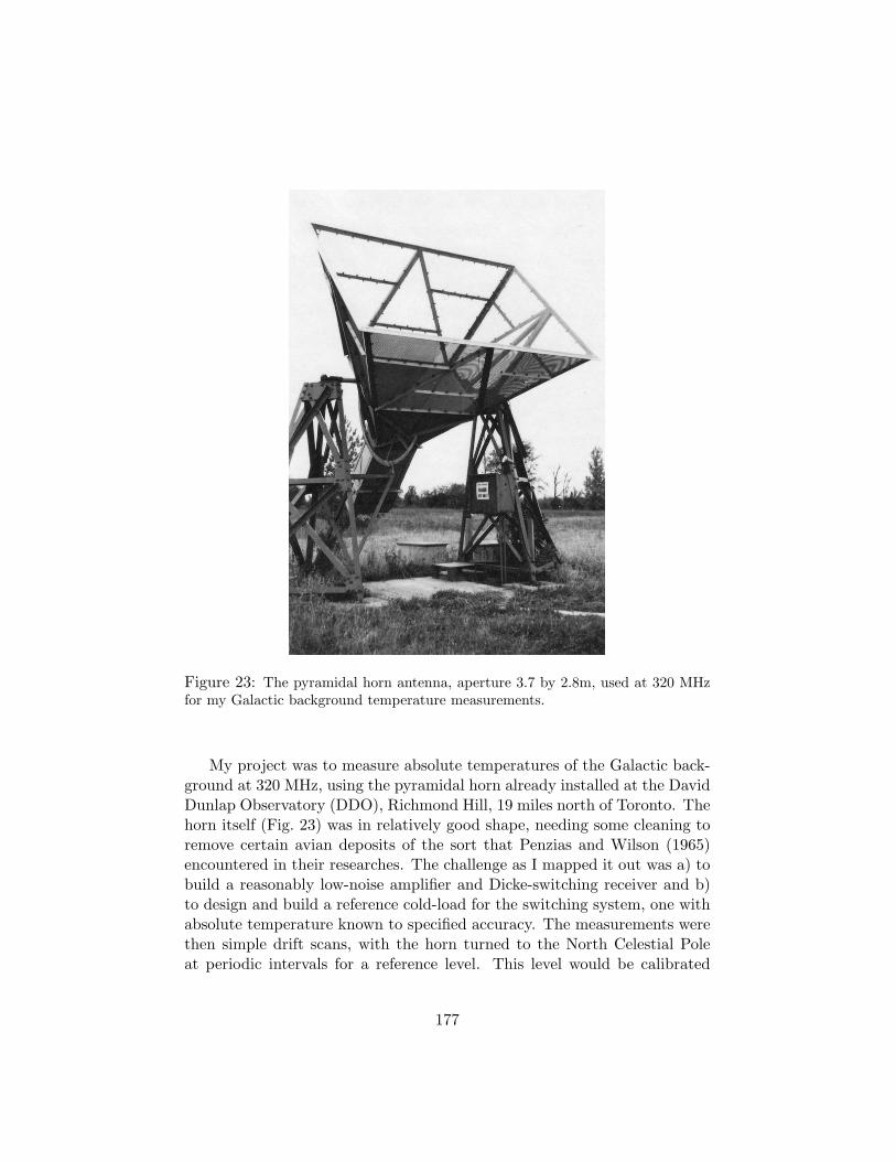
Figure 23: The pyramidal horn antenna, aperture 3.7 by 2.8m, used at 320 MHzfor my Galactic background temperature measurements.

My project was to measure absolute temperatures of the Galactic back-ground at 320 MHz, using the pyramidal horn already installed at the DavidDunlap Observatory (DDO), Richmond Hill, 19 miles north of Toronto. Thehorn itself (Fig. 23) was in relatively good shape, needing some cleaning toremove certain avian deposits of the sort that Penzias and Wilson (1965)encountered in their researches. The challenge as I mapped it out was a) tobuild a reasonably low-noise amplifier and Dicke-switching receiver and b)to design and build a reference cold-load for the switching system, one withabsolute temperature known to specified accuracy. The measurements werethen simple drift scans, with the horn turned to the North Celestial Poleat periodic intervals for a reference level. This level would be calibrated

177

by replacing the horn input with the reference cold-load input. There wereimpedance-matching subtleties involved, as long-serving radio astronomerswill recognize.

First task – to build a new receiver at 320 MHz. Field e!ect transistors,FETs, had just become available, actually working at this high a frequency!Low noise as well! But they cost real money, all of $34 each. In a rareinterview with Allan, I got the money, and the transistor. Next day I blewit up. (In retrospect I begin to understand the supervisor problem.) Imanaged to extract funds for a second one, and after walking around it foran afternoon, made a decision on how to handle it which helped me therest of my life. It’s just another transistor! Handle with ordinary care -otherwise I couldn’t see how I’d get anywhere. It worked. I applied thelesson later when dealing with original astronomical plates. Treat them asyou treat glass, with respect, but without awe. More tense and more ‘careful’( greater risk and less research.

The second FET ran throughout the project. The new receiver wasbuilt with help of George Watson, a solitary soul working out at RichmondHill: a craftsman, a perfectionist and a delight, whose stories, unrepeatableand certainly unprintable, enlivened many of my days and nights in thelittle frozen cabin at Richmond Hill, while adding a certain breadth to mygraduate education. More supervisor trouble ensued when in the course oftransporting a frequency generator to the cabin (they weighed about 150 kgin those days), I settled the old radio-astronomy station wagon axle-deepinto the Observatory grounds in soft spring mud.

The cold load was a real challenge. Nobody really knew how to proceed,and the one I fashioned was the best technical achievement of my MSc. Itdid work well, and I was confident of its noise temperature - but note thatit was a liquid nitrogen cold load, at about 80K. This was close to themean Galactic brightness temperatures; but of course a long way away fromCMBR values.

I heard/read of the CMBR as my observations progressed. Reaction(a): nothing to do with me; I’m a Galactic (semi-) astronomer, working attoo low a frequency and too high a mean brightness. Reaction (b), withminimal cosmic consciousness and from a radio astronomy point of view:surprise, Ryle was right after all – but a singular beginning? Steady statewas conceptually much easier to handle...

And following this 2 minutes of deep thought, back to reality – thehorn antenna had half-power beamwidths of 19.0"%22.5" degrees. Absolutetemperature mapping requires correction for the response in side and backlobes, of course. Thus I built a scaled version of the horn, complete with

178

Figure 24: A chunk of drift scan, this one at declination ) = 40" com-plete with periodic visits to the North Celestial Pole and calibration-signalinjections.

supporting structure, smaller by a factor of 9 and operating at 2.88 GHz. Imounted this on the antenna range turntable on the roof of the ElectricalEngineering building, with a distant horn reflector plus S-band generatorto provide the signal. The main-beam and first sidelobe patterns agreedremarkably well with the main-beam measurements of the main horn usingdrift scans of the sun, a point source (only 30 arcmin in size!) to the fatbeam of the horn. The side and back lobes enabled me to estimate thespillover radiation.

There were many delays, including my MSc course load and stormywinter weather. Measurements began in February 1965 and continued toJune; I covered the hottest part of the sky but by June (Fig. 24), interferencefrom the USAF Bu!alo base essentially halted the observations. I could notfinish the cold (Galactic anticentre) parts, another sore point between meand supervisors. My MSc thesis, complete with the iterative calculations toremove side and back-lobe responses, was completed in October 1965. Inparallel Donald Chu ran a sister set of measurements at 707 MHz, usinga 2.5 m precision horn reflector at the Algonquin Radio Observatory of theNational Research Council of Canada. The techniques he used followedmine precisely, including construction of a scaled model of the horn reflector.His measurements and mine were to be used to calibrate in absolute termshigher-resolution Galactic Plane surveys at DDO with a new 10m paraboloidreflector (for which I did commissioning and feed design.) These togetherwith polarization measurements which Ernie Seaquist was working on wereto provide comprehensive data on the Milky Way emission. This grander

179

scheme never happened.In November I set o! for Australia, where I had been o!ered a scholarship

at the Australian National University to do a PhD in a collaborative radio-optical programme between Mount Stromlo Observatory and the AustralianNational Radio Astronomy Observatory at Parkes. John Bolton was to bemy supervisor. My seduction by astronomy was complete. Engineeringcropped up later in life in building CCD systems, commissioning telescopesetc; but it was astronomy now where my commitment lay.

Donald Chu, finishing the same patch of sky I had done, likewise leftfor di!erent things, a proper job in his case with the then largest computercompany.

In the excitement of starting a new life in a country where snow driftsacross the telescopes were no longer a problem, the brightness temperaturemeasurements were temporarily laid aside.

The rest of the story has a certain inevitability about it. Donald Chuhad made some tentative comparisons of his data with mine; he found un-satisfactory answers. We knew roughly what the emission spectrum of theGalactic background was - this synchrotron emission continuum from long-blown supernovae had a brightness spectral index of about !0.5 to !0.7(Yates and Wielebinski 1967). Comparison of the 320 – 707 MHz results atindependent map points by Donald and myself yielded a spectral index of!0.3, far too flat. Trying to reach indices in the ‘recognized’ range meantzero point errors outside our estimates. In 1965 we had left it at this: we’dboth moved on.

In 1967 or 1968, as cosmological consciousness dawned, I realized whathad happened. Subtracting 3K from both our sets of measurements yieldedspectral indices in agreement with the ‘known’ results (Fig. 25). I collectedthe data together, re-digitized it, and finally wrote up the experiments (Wall,Chu and Yen 1970). There was no great urgency at this stage.

In retrospect a dedicated CMBR measurement would have been simple.We had only to cover the colder parts of the sky, put our two sets of mea-surements together with a prior on the Galactic emission spectral index,and a measurement of the excess radiation was there. We were a bit latein the time frame — but if we’d got on with it in the first years of ourMSc degrees rather than spending them wading through forgotten courseson plasma physics, the result was waiting for us.

The most astonishing aspect to me in hindsight was just how easy itwould have been to make the measurement successfully, using the horns wealready had, and a financial outlay of almost nothing.

I blame VLBI (partially). If Allan Yen had not become preoccupied with

180

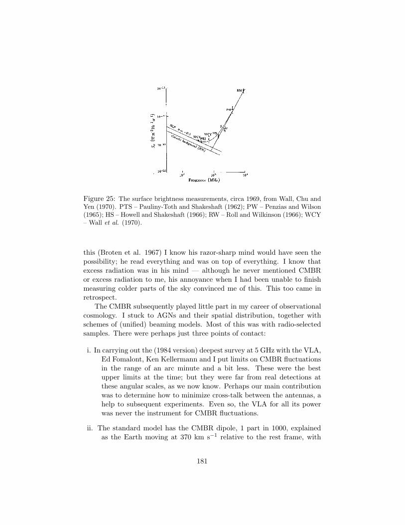
Figure 25: The surface brightness measurements, circa 1969, from Wall, Chu andYen (1970). PTS – Pauliny-Toth and Shakeshaft (1962); PW – Penzias and Wilson(1965); HS – Howell and Shakeshaft (1966); RW – Roll and Wilkinson (1966); WCY– Wall et al. (1970).

this (Broten et al. 1967) I know his razor-sharp mind would have seen thepossibility; he read everything and was on top of everything. I know thatexcess radiation was in his mind — although he never mentioned CMBRor excess radiation to me, his annoyance when I had been unable to finishmeasuring colder parts of the sky convinced me of this. This too came inretrospect.

The CMBR subsequently played little part in my career of observationalcosmology. I stuck to AGNs and their spatial distribution, together withschemes of (unified) beaming models. Most of this was with radio-selectedsamples. There were perhaps just three points of contact:

i. In carrying out the (1984 version) deepest survey at 5 GHz with the VLA,Ed Fomalont, Ken Kellermann and I put limits on CMBR fluctuationsin the range of an arc minute and a bit less. These were the bestupper limits at the time; but they were far from real detections atthese angular scales, as we now know. Perhaps our main contributionwas to determine how to minimize cross-talk between the antennas, ahelp to subsequent experiments. Even so, the VLA for all its powerwas never the instrument for CMBR fluctuations.

ii. The standard model has the CMBR dipole, 1 part in 1000, explainedas the Earth moving at 370 km s!1 relative to the rest frame, with

181

Figure 26: Left: measured amplitudes of the deviation from mean surface densityfor NVSS sources, as a function of right ascension. (Note that the direction of theCMBR dipole lies – accidentally – close to the Celestial Equator.) The predictedamplitude is shown as the solid line. Right: error circles (1*, 2*) representing thedirection of the NVSS dipole for samples selected at di!erent flux-density levels.The point denotes the direction of the CMBR dipole.

apparent temperature brighter in the direction of motion. The pre-dicted motion should be visible in the number counts of distant ob-jects, their combined surface brightness enhanced in the direction ofmotion of the earth. There are serious di"culties in looking for thisdipole in discrete objects: how distant, how to select, how to per-form widescale calibration; what to do about obscuration, how to getbeyond the cluster-dominated epoch. A uniform all-sky survey of ra-dio sources o!ers hope, however, as Ellis and Baldwin (1984) pointedout. After completion of the superb NRAO VLA Sky Survey (NVSS;Condon et al. 1998), that hope could be really entertained. It tookmuch work to understand the systematics of the survey, and muchwork to remove the nearby objects from it — but in the end ChrisBlake and I succeeded in observing the dipole (Blake and Wall 2002),agreeing in magnitude and direction with Earth motion as implied bythe CMBR (Fig. 26). This remains the only detection of the velocitydipole in discrete galaxies, objects formed long after the epoch at red-shift z $ 1100 corresponding to the last scattering surface from whichwe see the CMBR. The mean redshift of our radio galaxies is aboutunity. The Universe is therefore showing large-scale homogeneity atthis epoch, and further analyses coupled with new deep and wide skysurveys can refine this result. Although few doubt the interpretation

182

of the dipole in the CMBR, the detection in real objects representsone of the tests the CMBR needs to pass if it is truly a relic of the BigBang (Ellis 2002).

iii With superb results from WMAP (Bennett et al. 2003), and with thePlanck mission on the horizon, we would like some reassurance thatthe fluctuations we see in the CMBR are not contaminated by extremeinverted-spectrum populations of radio-mm sources. To this end, withRick Perley, Robert Laing, Joe Silk and Angela Taylor, I recently pro-posed a 43-GHz VLA survey of some 2 square degrees of the northernsky to search for such a population. This is the highest frequencysearch for extragalactic radio sources – and it found very few (Wallet al. 2006). We conclude that at small angular scales and the highfrequencies of the power spectrum of the fluctuations in the CMBR,have little to fear from discrete-radio-source contamination.

I o!er some conclusions.

1. The CMBR was there all the time in our 1965 data; and we could havedone the measurements earlier with specific attention to detecting it asa part of our absolute measurements. It would have come in somewherebetween 3 and 5 K at a guess. I think it’s a stretch to say that we wouldhave believed it on its own; our frequencies were a little low. But hadthere had been contact with cosmologists such as between Penzias andWilson (1965) and Dicke, Peebles, Roll and Wilkinson (1965), then itmight have been di!erent. Too if my cosmic consciousness had notdawned so slowly, it might have been di!erent.

2. I cannot have any regrets. My MSc project was superb for startingresearch in observational astronomy. How better to learn everythingabout the basics of radio astronomy? Every aspect in the processwas revealed to me in glaring detail, all the pitfalls, noise, bandwidth,line-loss, mismatch, spillover, ground radiation, antenna patterns, con-version of antenna temperature to brightness temperature... it wasbaptism by fire, and I did love it, I think. It is next to impossiblefor a student nowadays to learn about instrumentation in depth atany wavelength, and I grudge a big vote of thanks to my supervisorsDonald MacRae and Allan Yen for so comprehensively dropping meinto it.

3. It is possible to observe and not see. After all Donald Chu and I wereonly a couple of engineers playing around with horn antennas...

183

John Shakeshaft: Early CMBR Observations at the Mullard RadioAstronomy Observatory

John Shakeshaft is an Emeritus Fellow at St Catharine’s College, Cam-bridge. He served for many years as an Editor of Monthly Notices of theRoyal Astronomical Society

At the time of publication of the Penzias and Wilson (1965) paper, I was amember of sta! in the Radio Astronomy Group of the Cavendish Labora-tory, the physics department of the University of Cambridge, having beenan undergraduate and graduate student at Cambridge, the latter under theinspiring supervision of Martin Ryle. I had had an interest in cosmology andmeasurements of cosmic radio radiation for over ten years. Indeed my firstpublished scientific paper, in 1954, had the title The Isotropic Component ofCosmic Radio-frequency Radiation, although I advise readers not to botherto search it out. At that date, low-noise receivers for the microwave rangehad not yet been developed, so interest was concentrated at lower frequen-cies. Westerhout and Oort (1951) had shown that the survey of galacticradiation at 100 MHz (or Mc/sec as we called it) by Bolton and Westfield(1951) could be explained by assuming that most of the radiation came from“radio stars” distributed through the Galaxy in the same way as the commonPopulation II stars of types G and K, although it was necessary to add inan isotropic component besides. They suggested three possible explanationsfor this extra component but found none to be satisfactory. Subsequent totheir paper, extragalactic sources much more intense than normal galaxieshad been identified, such as the so-called “colliding galaxies” Cygnus A, andI attempted an estimate of the integrated contribution due to these. Inter-estingly perhaps, in view of later controversies about the number-counts ofradio and their cosmological significance, I concluded that the isotropic com-ponent could be accounted for by standard relativistic cosmological modelsbut not by the steady state theory. Shortly after publication, however, thegeneral realization that galactic radio emission is largely due to synchrotronradiation from cosmic ray electrons in the interstellar magnetic field vitiatedboth the Westerhout and Oort model and my conclusion from it.

Towards the end of that decade I began work, with graduate studentIvan Pauliny-Toth, on a survey of the background radiation at 404 MHz(! = 74 cm). This was intended as part of a study over a range of fre-quencies to determine the spectrum of the galactic radiation as a functionof direction, which could provide information on the dependence of cosmicray electron density and interstellar magnetic fields on position within theGalaxy. It was therefore important, if brightness temperatures at di!erent

184

frequencies were to be compared, for these temperatures to be absolute val-ues rather than merely relative values in di!erent directions. We used an 8-mdiameter dish on an alt-azimuth mount (it was in fact a German radar dish“liberated” after the Second World War by Martin Ryle, and one of the twodishes that Graham Smith used as an interferometer to determine accuratepositions of the sources Cygnus A and Cassiopeia A, enabling their opticalidentifications by Walter Baade and Rudolph Minkowski), an electron beamparametric amplifier and a Dicke-type radiometer with a liquid nitrogen ref-erence source. The published survey (Pauliny-Toth and Shakeshaft 1962)was used later both at Cambridge and elsewhere to correct CMBR measure-ments for the contribution due to galactic radiation The experience gainedon determining losses in the antenna and connections, and ground radiationin the far-out sidelobes, was also helpful in measurements of the CMBR afew years later.

The news in 1965 of the serendipitous result from Holmdel of 3.3 KCMBR at 4080 MHz (the second such major astronomical discovery fromthere, the first being Karl Jansky’s accidental finding of the galactic ra-dio emission in 1931) was received at the Mullard Observatory with greatinterest but no real surprise, since our work on radio source surveys overthe previous 12 years had left us convinced that the Universe was evolv-ing and not in a steady state; the discovery of radiation from a big bangtherefore fitted naturally with these ideas. Although the data from the 2CSurvey had been over-interpreted in terms of actual sources, the ingeniousP (D) probability analysis by Peter Scheuer (1957) of the deflections D ofthe interferometer records themselves, without the identification of individ-ual sources, showed conclusively (to us, at least) that the slope of the radiosource counts N() S) was proportional to S!1.8, significantly steeper thanthe N() S) proportional to S!1.5 expected for a uniform Euclidean model,and even more so than the values expected for Friedman and steady statemodels. By 1965, the increase in the numbers of actual identifications ofdistant radio galaxies and quasars had confirmed the excess of sources atlarge redshifts, and subsequent studies have shown that Scheuer’s result forthe slope was indeed correct. One of the merits of the steady state theorywas said to have been that it gave specific predictions, unlike the Fried-man models, but its proponents seemed very reluctant to accept that thesepredictions were in conflict with the observations.

I realized that we were in a position fairly easily to check the Holmdeltemperature value at a di!erent frequency, namely 1407 MHz (! = 21.3 cm),which would help to determine whether this component of radiation hada thermal spectrum as predicted. With the aid of graduate student Tim

185

Howell, a copper horn of beamsize 13" % 15" was set up inside the 8-m dishmentioned above, itself surrounded by a wire mesh screen, 30 m square,lifted at the edges, so the horn was doubly screened from ground radiation.The horn was connected to a Dicke radiometer, with a termination in liquidhelium as the reference source. This consisted of a metal film resistor at theend of a 75-cm length of low-loss coaxial line. The temperature distributionalong the line was measured and the e!ective noise temperature at the upperend calculated to be TL = 5.9±0.2 K. When the leads from the horn and coldload were interchanged in the circuit, the alteration of receiver output gavea direct measure of the temperature di!erence with no contribution fromany asymmetry of the switch and leads. The receiver output was calibratedby measuring the di!erences between terminations immersed in water atvarious temperatures.

Observations were made at night with the horn directed towards thezenith (declination ) = 52") at a right ascension such that the galactic radioemission was at a minimum. A temperature di!erence TH ! TL = 0.9 ±0.1 K was found, implying that TH = 6.8± 0.3 K, representing the combinedcontributions from (a) galactic radiation and the CMBR, (b) atmosphericemission, (c) ground radiation, and (d) losses in the horn and waveguide-coaxial connection. For (b) we took the value of 2.2 K, derived by Dave Hoggfor a wavelength of 20.7 cm (see below), and assumed an error of ±0.2 K. For(c), we measured the polar diagram of the horn and estimated a value lessthan 0.1 K, and for (d) we calculated a contribution of 1.3± 0.2 K. The sumof (b), (c) and (d) was 3.5 ± 0.3 K, leading to a value of 3.3 ± 0.5 K for theminimum background brightness temperature. The galactic contribution tothis was found by convolving the reception pattern of the horn with thebrightness temperatures measured in the survey at 74 cm mentioned earlierand scaling the result to 20.7 cm by assuming T to be proportional to !2.7.22

The result was 0.5 ± 0.2 K, leaving a CMBR value of 2.8 ± 0.6 K (Howelland Shakeshaft 1966), which turns out to be gratifyingly — if fortuitously— close to the currently accepted value of 2.725 K.

The atmospheric absorption for frequencies up to 8 GHz is due pre-dominantly to non-resonant absorption by molecular oxygen, and Hogg

22To my embarrassment, Jim Peebles, in reviewing this piece, has noticed that the actualwavelength corresponding to a frequency of 1407 MHz is of course 21.3 cm rather than20.7 cm, as appeared in the original paper and as I unthinkingly copied above. He is thefirst person in the last 40 years to have pointed out this blunder to me. At this late dateI do not have the original working material available and so cannot determine whetherthe quoted temperature of 2.8±0.6K might require modification. Any such change wouldonly be in the second decimal place, already omitted due to the size of the error.

186

(1959) had calculated values from 400 MHz up, on the assumption of aline-broadening constant of 0.75GHz per atmosphere. Our search of theliterature for experimental measurements of the absorption by observationsof the extinction of extra-terrestrial sources as a function of zenith angle hadrevealed a relatively wide scatter of values, with some in very poor agreementwith Hogg’s predictions. To throw more light on this problem, we carriedout measurements of our own at 408 and 1407 MHz. The interpretation ofthese involved consideration of the change of apparent angular size of thesource in question due to di!erential refraction in the atmosphere. Afterapplying the necessary corrections, our results fitted well with Hogg’s curve,but we then realized that some of the earlier workers had either not appliedthe refraction correction or had applied it with the wrong sign. Judicious re-working of the earlier results, where necessary, then produced a satisfactoryagreement between theory and experiment (Howell and Shakeshaft 1967a).

On completion of the initial measurement of the CMBR at 1407 MHz, wetried to check whether this component of the cosmic radiation could be de-tected at the lower frequencies of 408 and 610 MHz, although the dominanceof galactic radiation in this range would cause increased uncertainties. Stud-ies by Peter Scheuer (1975)23 and by Ray Weymann (1966) had suggestedthat deviations from a blackbody spectrum might be present at low frequen-cies. We used optimal scaled horns with beamwidths of 15", screened fromground radiation by wire mesh, and Dicke radiometers with liquid heliumreference sources as before. After applying corrections for other contribu-tions as at 1407 MHz, the e!ective brightness temperatures from the regionof the celestial North Pole were 24.3 ± 0.9 K at 408 MHz and 10.4 ± 0.7 Kat 610 MHz, the ratio of these, 2.3 ± 0.2, being significantly less than theratio of 3.1 ± 0.1 expected for the galactic contribution with a temperaturespectral index of !2.8 (T " !2.8). This implied that there was indeed anextra component of radiation characterized by a temperature close to in-dependent of wavelength, that is, a blackbody spectrum. Further analysisindicated that, if the spectrum of this component were blackbody, the excesstemperature would be 3.7 ± 1.2 K (Howell and Shakeshaft 1967b). Unfor-tunately, the error in this value was such that no new upper limit could beput on the epoch of ionization of the intergalactic gas.

This work concluded for over twenty years observational studies at theMullard Radio Astronomy Observatory of the CMBR, since other groupsmuch better equipped for work at high frequencies had vigorously entered

23Presented in an article written in 1965 for Galaxies and the Universe, and eventuallypublished in revised form in 1975

187

the field, but they were subsequently taken up again with the building byPaul Scott and others of the Cosmic Anisotropy Telescope (CAT), a three-element interferometer which, in 1996, was the first telescope to detect struc-ture in the CMBR on angular scales smaller than the main peak in the angu-lar spectrum (Scott et al. 1996). This was followed by the Very Small Array(VSA), now observing from Tenerife the anisotropies on angular scales be-tween 15 arcminutes and 2 degrees, and the Arcminute MicroKelvin Imager(AMI) to study the Sunyaev-Zeldovich e!ect in high-redshift clusters andproto-clusters of galaxies. In addition to this observational work, there hasbeen theoretical modelling of background fluctuations, and the CambridgePlanck Analysis Centre has been set up in preparation for the launch in2008 of the European Planck Surveyor satellite.

Other authors in this volume have noted that, if the attention of obser-vationalists had been drawn to the matter, the CMBR could perhaps havebeen detected (or recognized as such) years earlier than in fact it was. Itis, for example, unfortunate that in neither of the two editions (1952 and1960a) of his influential textbook Cosmology did Hermann Bondi refer tothe possibility, nor did Fred Hoyle in his paper The Relation of Radio As-tronomy to Cosmology at the Paris Symposium on Radio Astronomy (1958).We must hope that su"cient of the astronomical literature is now availableon the World Wide Web for rapid searches which could prevent oversightsof this kind in the future.

188

William “Jack” Welch: Experiments with the CMBR

Jack Welch retired from teaching Astronomy and Electrical Engineering atUC Berkeley in 2005 but continues as the Alberts Professor in the Searchfor Extraterrestrial Intelligence. He was Director of the Radio AstronomyLaboratory at Berkeley from 1972 to 1996 during which time the BIMAMillimeter Telescope array was built and operated. He continues his researchin the interstellar medium and star formation and is curently working oncompletion of the Allen Telescope Array.

My introduction to the question of the absolute radio brightness of the skycame from a talk that I heard at a meeting of the IEEE Antennas and Prop-agation group held in Palo Alto in 1961 or 1962. The Speaker was R. W.De Grasse, one of the team of engineers at the Bell Telephone Laborato-ries that had developed a communication system for the Echo project. Hedescribed the horn-reflector antenna and maser receiver amplifier that hadbeen built at Crawford Hill in New Jersey. As a young radio engineer justbeginning work in radio astronomy at Berkeley, I was enormously impressedwith the quality of the instrumental work and the care taken with the sys-tem noise measurements. I remember him saying that they assumed the skybackground temperature to be zero but were uncertain about an excess of acouple of degrees or so in their summary of system noise contributions. Theexcess was thought to be pick-up in the antenna sidelobes (Ohm 1961). Atthe time, I had no idea what to expect for the background.

A few years later, I read the Astrophysical Journal letter by Penziasand Wilson (1965) describing their beautiful background measurements withthat same antenna. Using a new receiver at 4.08 GHz with a new referenceload (Penzias 1965), they were able to report with certainty an excess ofabout 3.5 K that had to be ascribed to the cosmic background. The compan-ion paper by the Princeton group (Dicke, Peebles, Roll and Wilkinson 1965)with the plausible interpretation that the radiation was the blackbody radi-ation remnant of an earlier stage of an expanding universe was very exciting.George Field, who had recently joined the Berkeley Astronomy Department,was very taken with the new finding and realized that earlier observations ofthe excitation of interstellar CN (Herzberg 1950) might be consistent withthe new radio observations. The excitation of the first rotational level of theCN line corresponded to background radiation at a wavelength of 2.6 mm,suggesting that the excess radiation was that of a blackbody in agreementwith the Princeton group interpretation. At the time, our group was devel-oping receiving equipment at wavelengths near 1.0 cm for radio astronomyand studies of atmospheric emission with a small antenna. George urged us

189

to attempt a measurement of the cosmic microwave background radiationto help determine its spectrum at the shorter wavelengths.

We decided to take a detour from our other program to study the back-ground at a wavelength of 1.5 cm. An important piece of information aboutthe universe had been found. We might be able to add to that, and it wouldbe an interesting instrumental challenge. At 1.5 cm wavelength, the back-ground emission from the atmosphere is rather high at sea level sites, andwe planned an observation from the High Altitude Barcroft Laboratory ofthe University of California White Mountain Research Station. Sam Silver,the Director of the Space Sciences Lab at the University of California, hadoutfitted a trailer for remote observations, and we were able to take it to theBarcroft Laboratory for our observations. The atmospheric emission bright-ness is typically only 3 to 4 K at the 12,400 foot altitude of the BarcroftLaboratory. Our technique was conventional. We used a Dicke radiometerthat compared the brightness of the sky as detected by a standard gainhorn and associated receiver with that of blackbody loads at known tem-peratures, and we made tipping measurements to extrapolate the brightnessto zero air mass. One di!erence in our system was that we used a load atthe temperature of liquid nitrogen as our low temperature reference ratherthan a liquid helium load. We felt that we could characterize it well and itwould be easier to manage at the remote site than a liquid helium load suchas those used by the other groups. As a check, we measured a liquid heliumload in the lab at Berkeley with our system and found the correct tempera-ture. We spent the summer of 1966 making background observations at thehigh altitude site.

Our reported result, 2.0 ± 0.8 K, was disappointing (Welch, Keachie,Thornton and Wrixon 1967). The final uncertainty was large. The re-producibility of individual measurements was limited by the scatter in themeasurements of the liquid nitrogen load brightness. Because of the greatertemperature di!erence between the sky brightness and that of liquid ni-trogen, the extrapolated results were subject to greater random errors. Inaddition, our mean value was low in comparison with the results of the othermeasurements available at the time of our publication. The average, par-ticularly including the first radio detections (Penzias and Wilson 1965; Rolland Wilkinson 1966) and the temperatures derived from CN measurements(Field and Hitchcock 1966; Thaddeus and Clauser 1966) were pointing toa blackbody temperature of 3.0 K or even higher, outside our error limit.As the more accurate measurements, shortly thereafter from the Wilkin-son group (Partridge and Wilkinson 1967) and others, and finally from theCOBE satellite (Mather et al. 1990) came in, we were somewhat relieved

190

that the limit of our error just included the final blackbody temperature,2.74K.

A year or so after our publication, I was reexamining the characterizationof the pyramidal horn for some other calibrations that we were planning anddiscovered that I had made a mistake in the model tipping curve that wehad used for the background measurements. Correcting for that properly,we would have had 2.3 ± 0.8K for our result, a little closer to the finalaccurate temperature. Since that miscalculation was small compared to ourrandom errors, we did not think it appropriate to publish it. In retrospect, Irealize that was a mistake. The systematic error is, of course, di!erent fromthe random errors, and it should have been reported.

We subsequently returned to our original program of getting a shortwavelength telescope running for other astronomical observations, particu-larly for studies of solar system objects and the interstellar medium. Therewe had some nice results with the first discoveries of polyatomic molecules inthe interstellar medium revealing the molecular clouds where stars are born(Cheung et al. 1968, 1969). Then we proceeded to develop interferometryat the short wavelengths for interstellar medium and star formation studiesas well as for other fields.

Our most recent encounter with CMBR studies occurred when we discov-ered that we were making some accurate ground-based flux measurements ofJupiter at the same time that they were being made by the WMAP satellitein the course of its calibration (Page et al. 2003). We had just completedour study when the WMAP results were announced. Our measurement wasmade at a wavelength of 1.05 cm (Gibson et al. 2005), in between the twolongest WMAP receiver bands and close to the center of the Jovian ammo-nia inversion absorption band. Our accuracy for the Jovian flux was about1.5% and it fell nicely between the Jovian fluxes of the two adjacent WMAPobservations which had comparable accuracies. I think that everyone waspleased with the good agreement between these independent calibrations ofJupiter. Our result enabled us to get a fairly accurate measure of the upperJovian atmospheric ammonia abundance. Absolute calibration to 1-2% ac-curacy was essential for getting a good Jovian atmospheric model, and theWMAP results helped with that as well.

Some of the best memories from the earlier period were of discussionswith Dave Wilkinson, an experimentalist of extraordinary capability.

191

Paul Boynton

to come...

192

Robert A. Stokes: Early Spectral Measurements of the CosmicMicrowave Background Radiation

Robert Stokes is President and CEO of Versa Power Systems, a solid-oxidefuel cell development company in the Denver, Colorado area. After com-pletion of his Ph.D. at Princeton in 1968 he received an appointment as anassistant professor at the University of Kentucky where he continued work onthe CMBR. Later he managed the engineering physics division at Battelle,Pacific Northwest Laboratories, served as Deputy Director of the NationalRenewable Energy Laboratory, and was Senior Vice President at the GasTechnology Institute.

As an undergraduate student at the University of Kentucky in the 1960s, Iwas part of a generation with a growing interest in space science encouragedby the US educational system’s response to the Soviet launch of the Sputniksatellite. At the end of my junior year I was selected to attend one of thefirst Goddard Institute summer study courses in space science at ColumbiaUniversity organized by Robert Jastrow. After an intense summer of fo-cusing on planetary astrophysics, our group was treated to a memorabletour of several US space science facilities, traveling aboard a chartered DC6aircraft in August of 1963. The tour included visits to the NSF astronomi-cal observatory at Kitt Peak, Arizona; the Marshall Space Flight Center inHuntsville, Alabama (the tour conducted by none other than Werner VonBraun); the NASA launch facility at Cape Canaveral; and NASA headquar-ters in Washington, DC. As a result, my interest in space science was greatlyintensified, and when presented with the opportunity to attend graduateschool at Princeton, a focus on space science was a foregone conclusion.

After a year of graduate study at Princeton and a couple of stimulatingclasses taught by John Wheeler, I managed to land a summer appointmentworking as a student research assistant for Bob Dicke and Mark Golden-berg, taking data on a special ground-based telescope designed to measurethe solar oblateness as a test of the predictions of the Brans-Dicke theory.That summer, Paul Henry, another graduate student, and I traded o! mak-ing observations while observing practice by the Princeton hammer-throwathletes, hoping all the time that our apparatus would not be damaged by amis-thrown 16-lb steel ball. By the end of the summer I had become a partof the graduate student cadre associated with the gravity group, led by Dickeand Wheeler and including their junior colleagues Peter Roll, Jim Peebles,Dave Wilkinson, Mark Goldenberg, Kip Thorne, and Bruce Partridge.

Jim Peebles had already begun some theoretical work on the implicationsof a hot-fireball model for the early universe and the nature of any remnant

193

radiation. Earlier modeling work by Alpher and Gamow (Alpher, Betheand Gamow 1948) and measurements of atmospheric radiation by Dicke,Beringer, Kyhl and Vane (1946) had laid the groundwork for the research notpursued in earnest until the mid-1960s. But by 1965, Peter Roll and DaveWilkinson had already begun operation of a 3-cm radiometer specificallydesigned to test the blackbody radiation hypothesis.

By the time the Princeton group had connected up with Arno Penziasand Bob Wilson at Bell Labs and published the famous 1965 companion pa-pers (Penzias and Wilson 1965a; Dicke, Peebles, Roll and Wilkinson 1965)on the cosmic microwave background radiation, I had just completed myPh.D. qualifying exams and was looking for a dissertation topic. Roll andWilkinson (1966, 1967) had sent their their confirming radiometric measure-ments to Physical Review Letters in January of 1966 and there was greatinterest in investigating the spectral nature of the newly discovered isotropicmicrowave radiation.

Dave Wilkinson agreed to take me on as his first doctoral student atPrinceton and set me to work building a 1.58-cm radiometer to make co-ordinated measurements with two radio telescopes he and Bruce Partridgewere constructing for a second series of measurements at 3.2 cm and 8.56mm. We had made arrangements to conduct several months of measure-ments at a high-altitude laboratory operated by the University of Californiaat Berkeley in the White Mountains along the California/Nevada borderduring the summer of 1967 to establish a more precise temperature for thebackground radiation field.

The hypothesis that the microwave background radiation is, in fact, theprimeval fireball rests heavily on the spectrum being that of a blackbody.Measurements completed prior to 1967 had all been consistent with a spec-tral index ' = 2 over a considerable wavelength range in the Rayleigh-Jeansregion of a 3 K blackbody.

To be convinced one is seeing true blackbody radiation and not thatof a hot graybody, it is necessary to go to short wavelengths and look forthe curvature in the spectrum due to quantum statistical e!ects. In early1967, Dave Wilkinson, Bruce Partridge, Paul Boynton and I began a seriesof experiments aimed at refining the absolute radiometric techniques andextending the wavelength coverage to 3.3 mm, a wavelength su"ciently shortto di!erentiate between a true blackbody and a hot graybody.

Four Dicke radiometers were constructed by the group using similar de-signs at wavelengths of 3.2 cm, 1.58 cm, 8.56 cm, and 3.3 mm and taken tomountain-top observing sites to reduce atmospheric background. The 3.2-cm and 1.58-cm measurements were repeated to check the earlier work and to

194

Figure 27: Robert Stokes with a 3.3-mm Radiometer — Colorado 1968.

provide an accurate determination of the spectral index. The 8.56-mm and3.3-mm points were expected to show deviations from the frequency-squareddependence in the spectrum of a hot graybody, the deviations amounting to20 percent at 8 mm and 300 percent at 3 mm.

A great deal of experience was gained from the Roll and Wilkinson ra-diometer that was operated atop a building on the Princeton Universitycampus, and Dave Wilkinson in particular was able to build on his exact-ing electron g ! 2 Ph.D. work at Michigan (Wilkinson 1962) to design anapproach that dealt with systematic errors in the experiments. A numberof other articles in this volume provide a good bit of detail and photos ofthe experimental apparatus used by the Princeton group (e.g. the article byBruce Partridge starting on page 252), so I will not repeat the details here.

The 3.2-cm, 1.58-cm, and 8.56-mm experiments (Stokes, Partridge andWilkinson 1967; Wilkinson 1967) were performed at an altitude of 12,470feet at the Barcroft facility of the White Mountain Research Station, Bishop,California, during July and August of 1967. The 3.3-mm result (Boynton,

195

Stokes and Wilkinson 1968) was obtained in March 1968 from an altitudeof 11,300 feet at the NCAR High Altitude Observatory, Climax, Colorado.Figure 27 shows a photo of the author with the 3.3-mm radiometer at theClimax site.

Paul Boynton had completed a nuclear physics Ph.D. at Princeton (Boyn-ton 1967) and decided to stay on as a postdoctoral student in the gravitygroup. At about the time that Dave Wilkinson, Bruce Partridge and I de-parted for Mount Barcroft, California, via Yuma Arizon, Boynton starteddesigning and procuring parts for the new 3.3-mm Dicke radiometer thatwas to be employed for the follow-up series of measurements.

Whereas the microwave radiometer components for the longer-wavelengthradiometers were mostly commercially available items, the microwave mixersfor the 3.3-mm superheterodyne receivers were still very much a development-stage component in 1967. After my return from California, Boynton and Ispent several months attempting to procure or develop an acceptable mi-crowave mixer that would work at 90 GHz (3.3 mm). We visited severalmilitary development labs and received considerable help and loaned com-ponents from the Aberdeen Proving Ground sta! in pursuit of a workingradiometer in late 1967. At the beginning of 1968 we made the decision inconsultation with Dave Wilkinson to give up on locating a reliable microwavemixer and put together a portable laboratory to transport to Colorado sothat we could construct the detectors ourselves from GaAs wafers and gold-alloy sharpened cat whiskers. It seemed a lot like the early days of radioexperimentation, but it worked! However, for the Colorado observations, wetypically needed to change out the mixer once or twice during each of theall-night runs.

The choice of wavelengths for the radiometers was dictated by the loca-tion of atmospheric windows in the millimeter band. This absorption andsubsequent reemission are the result of closely spaced pressure-broadenedresonance lines that occur in the water molecule near 1.3 cm and 0.27 cmwavelength, and in the oxygen molecule near 0.5 cm and 0.26 cm wavelength.To further minimize atmospheric e!ects, measurements were performed athigh altitudes during times of low absolute humidity. In addition to theusual problems with absolute measurements, the cosmic background radia-tion spectral measurements were made more di"cult by the impossibility ofmodulating the signal due to its isotropy. Since the microwave backgroundsignal is the residue after one has accounted for everything else, control ofthe systematic e!ects and careful calibration were crucial.

The results of the four radiometer measurements made by the Princetongroup using these techniques were all consistent with a 2.7 K blackbody. A

196

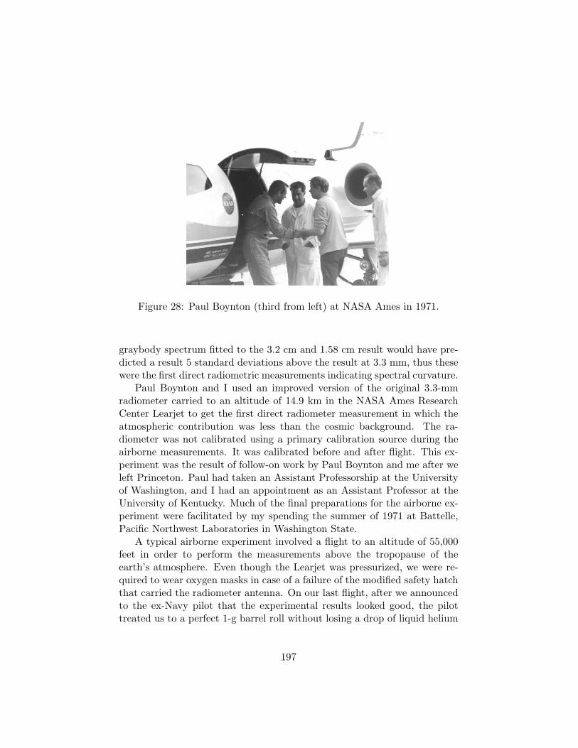
Figure 28: Paul Boynton (third from left) at NASA Ames in 1971.

graybody spectrum fitted to the 3.2 cm and 1.58 cm result would have pre-dicted a result 5 standard deviations above the result at 3.3 mm, thus thesewere the first direct radiometric measurements indicating spectral curvature.

Paul Boynton and I used an improved version of the original 3.3-mmradiometer carried to an altitude of 14.9 km in the NASA Ames ResearchCenter Learjet to get the first direct radiometer measurement in which theatmospheric contribution was less than the cosmic background. The ra-diometer was not calibrated using a primary calibration source during theairborne measurements. It was calibrated before and after flight. This ex-periment was the result of follow-on work by Paul Boynton and me after weleft Princeton. Paul had taken an Assistant Professorship at the Universityof Washington, and I had an appointment as an Assistant Professor at theUniversity of Kentucky. Much of the final preparations for the airborne ex-periment were facilitated by my spending the summer of 1971 at Battelle,Pacific Northwest Laboratories in Washington State.

A typical airborne experiment involved a flight to an altitude of 55,000feet in order to perform the measurements above the tropopause of theearth’s atmosphere. Even though the Learjet was pressurized, we were re-quired to wear oxygen masks in case of a failure of the modified safety hatchthat carried the radiometer antenna. On our last flight, after we announcedto the ex-Navy pilot that the experimental results looked good, the pilottreated us to a perfect 1-g barrel roll without losing a drop of liquid helium

197

from the calibration reference Dewar flask. Figure 28 is a photo of PaulBoynton and the pilot (left) just before takeo! on one of the flights.

Boynton and I published the airborne results in a letter to Nature (Boyn-ton and Stokes 1974). The measurement clearly showed the expected short-wavelength departure from the Rayleigh-Jeans spectrum. At this point anyquestions about the cosmological nature of the microwave background hadbeen put to rest, and attention shifted to detailed measurements of theanisotropies in the CMBR with the eventual launch of the Wilkinson Mi-crowave Anisotropy Probe on June 30, 2001, named in honor of Dave Wilkin-son who died in September 2002.

My subsequent career choices have taken me away from space science andcosmology to a focus on energy technology, however I continue to follow de-velopments in cosmology and space science as a highly interested individual.

198

Martin Harwit: An Attempt at Detecting the Cosmic BackgroundRadiation in the Early 1960s

Martin Harwit is professor emeritus of astronomy at Cornell University anda former director of the National Air and Space Museum. He is a Mis-sion Scientist on the European Space Agency’s Far-Infrared SubmillimeterTelescope project, Herschel, of which the National Aeronautics and SpaceAdministration is also a sponsor.

In 1963 I initiated an e!ort to look for the cosmic background radiationfrom space (Harwit 1964). The small research groups I started, first at theNaval Research Laboratory in Washington, DC, and later at Cornell Uni-versity, designed and constructed cryogenically cooled rocket telescopes todetect this radiation. My calculations showed that we would be hinderedby zodiacal foreground radiation. Our telescopes eventually confirmed this,by detecting the zodiacal glow along with a number of strong di!use Galac-tic sources. We also obtained painfully false results on the submillimetercomponent of the 3K microwave background radiation, due largely to emis-sion by contamination carried aloft by our rockets (Shivanandan, Houck andHarwit 1968). In order to depict the many mishaps, missteps and miscon-ception that motivated me to initiate background observations in the early1960s, I begin my account ten years earlier, when I was a graduate student.

In the spring of 1954 I found myself standing in the Physics Departmento"ce of Prof. David M. Dennison at the University of Michigan in AnnArbor. Dennison was an eminent molecular theorist. Sitting behind hisdesk, he was finding it di"cult to tell me that I would not qualify for a PhDin physics because I really had no aptitude for science. Perhaps I shouldlook at other occupations, because science clearly was not my metier.

Two months earlier, I had turned 23, and my career as a scientist alreadywas reaching an unfortunate conclusion. I had come to Michigan to studychemical physics. Although my undergraduate major had been physics, Ihad taken an advanced chemical physics course before coming to Michiganand read through Linus Pauling’s (1948) excellent book The Nature of theChemical Bond, and Gerhard Herzberg’s (1945, 1950) two books on molec-ular spectroscopy. The field looked genuinely exciting. At Michigan, I wasassigned to carry out near-infrared spectroscopic work on peptide bonds inthe laboratories of Prof. G. B. B. M. Sutherland, who later became Direc-tor of the National Physical Laboratories in Britain. During my one-yearapprenticeship, I learned a lot about infrared techniques but did not accom-plish much. I was studying for my doctoral exams at the time, and neither

199

the research nor the exams went well, which was why I was standing in Prof.Dennison’s o"ce that day.

Having to leave the Physics Department and wanting some time to figureout what to do next, I stayed on in Ann Arbor that summer, and found ajob in the laboratories of Prof. Leslie Jones in the School of Engineering.He and his group were conducting upper atmosphere research with rocket-borne instrumentation. I did some optical design with the group and tackledwhatever jobs needed doing. It was the first time I had real fun in science.

The war in Korea had not yet ended in 1954. In the fall of that yearI received the then-standard letter from my draft board, which began withthe ominous words, “Greetings from the President of the United States.”and explained how my “friends and neighbors” had selected me to serve inthe United States Army. I was to report for my two year stint of duty inJanuary 1955.

Because I had earned an MA in Physics at Michigan by this time, theArmy assigned me to the Chemical Corps at the Army Chemical Centerin Edgewood, Maryland. This is where I began my real scientific training.Most of the civil servants in the Corps were chemical engineers and knewlittle about physics. But now, ten years after the end of World War II, thegovernment was asking them to work on radioactive fallout, neutron dosesfrom nuclear bomb bursts, and similar problems. I found that with a fewvisits to the base library, I could usually figure out what needed to be done,and although I was just an army private, I was given a lot of responsibility.Nevertheless, my civil service supervisor would send me to places like MITor Woods Hole to verify with known experts that my calculations had beencorrect, and I enjoyed the opportunities o!ered by those visits.

In my second year in the Army, I was sent to Eniwetok and Bikini atolls inthe Pacific for a few months to participate in what at the time was believedto be the first hydrogen bomb drop from an aircraft. We attempted tomeasure neutron doses at di!erent distances from nuclear explosions, bigand small. Some of them could vaporize an entire island in the atoll, othersjust left a small crater. To while away the time between work and snorkelingin the waters of the atolls, I had taken along a number of books, among thema popular astronomy book by Fred Hoyle. I no longer recall whether it washis Frontiers in Astronomy or The Nature of the Universe. Both books wereout in paperback by that time, as were all the books I had taken along.Though Hoyle used no formulae and little technical language, I began tothink that I would be able to do the calculations he was describing. It wasquite fascinating.

At the end of my two years’ service, I applied to graduate schools and

200

was accepted by MIT, on the strengths of what must have been great recom-mendations from Leslie Jones, my supervisors at the Army Chemical Center,and one of the MIT professors the Army had sent me to consult.

At MIT, there was no course requirement in one’s major subject. Butfor a minor, a student was required to pass three advanced courses. I signedup for an astrophysics minor. It is hard to believe, today, but in 1957 MIThad no astrophysics curriculum. However, an exchange arrangement withHarvard permitted me to take three graduate courses there.

Tommy Gold had just been given a Harvard professorship. At the time,he was postulating that dust on the Moon would hop around in response toelectrostatic bombardment from the solar wind. Inspired by this, I beggedand borrowed some equipment in the MIT Laboratory of Electronics, learnedhow to blow glass so I could construct a vacuum tube for bombarding dustwith electrons, and then saw the dust disperse when I turned on the electronbeam. Tommy came down to MIT to see this late one evening. He wasdelighted and asked whether I might like to switch to astrophysics afterreceiving my PhD. I had done some calculations in one of his seminars, andhe thought I should post doc with Fred Hoyle. Of course, I was very pleased,though I still had my thesis work to complete.

I had come across the recently discovered Hanbury Brown / Twiss e!ect,and read the controversy surrounding it that aired in the journal Nature atthe time. Edward M. Purcell’s clean resolution of that controversy was par-ticularly illuminating. I thought that the techniques developed for detectingthe HB/T e!ect might provide a first opportunity to directly detect BoseEinstein fluctuations in electromagnetic radiation from a source in thermalequilibrium. None of the experimentalists in the MIT Physics Departmentwere particularly interested in my making these measurements, but Prof.William P. Allis, a leading plasma theorist, said he’d be willing to supervisethe thesis if I could find the means to build the requisite apparatus.

The Naval Supersonic Wind Tunnel located on the MIT campus at thetime was run by Prof. John R. Markham of the MIT Aeronautical Engineer-ing Department. One of the problems they were tackling was the detectionof the hot exhausts of rockets and jet engines. This necessitated devicessensitive to the infrared radiation from these plumes. Improved sensitivitycould be achieved by using not one detector, but two, and correlating theirsignals. This correlation technique was also needed for the Hanbury Brown/ Twiss apparatus. The Aeronautical Engineering Department o!ered tobuy as much of the requisite equipment as could be commercially obtained.They would use the apparatus during working hours, and I was free to useit for my thesis work at night. They generously also provided me with the

201

assistantship I would need to finish my thesis work.The fluctuations to be measured were minuscule, and detectors available

at the time were still quite insensitive, but by April 1960 I had reasonablyreliable results, and was finished with my thesis (Harwit 1960). Early inMay, my wife Marianne and I embarked on the USS United States for me tospend a NATO sponsored postdoctoral fellowship year with Fred Hoyle inCambridge. Four years earlier, I had been inspired by his popular writing.Now, I would be working with him. I hardly believed my good fortune!

When we arrived in Cambridge, Fred was away on one of his prolongedvisits to Caltech, and I had time to finish a paper I had begun while still atMIT. I had found a small error in a paper on galaxy formation in a steadystate universe by Dennis Sciama. When I redid the calculation, it showedquite clearly that there was no way that a steady state universe could formgalaxies at the replenishment rate required by the expansion of the Universe,unless forces other than gravitation were at play.

I submitted the paper to the Monthly Notices of the Royal Astronomi-cal Society, and some time later received an acceptance and an invitationto present the work at one of the monthly meetings in Burlington House(Harwit 1961). To my dismay, a week before my scheduled talk, I saw anannouncement on one of the Cavendish Laboratory’s bulletin boards thatHermann Bondi, one of the original creators of the steady state theory, wasgoing to give a talk at Kings College, London, on precisely the same topicof steady state galaxy formation the week after my talk at the RAS. I hadheard that Bondi was a fierce debater. As secretary of the RAS he wouldundoubtedly be present at my talk. I expected a punishing onslaught, and atonce began to prepare myself by reading everything Bondi had ever writtenon related subjects.

On the day of the meeting, I gave my talk, sparred with Bondi, butfelt that I had acquitted myself reasonably. At the end of the session, Iapproached Bondi and introduced myself. At his suggestion we went to eata hamburger and chat for a while before he had to take the train home toSussex and I returned to Cambridge. He told me he had been the refereeon my paper which had suggested some further work to him. Would I havetime to come to Kings College the following week to hear his talk? I wasdelighted, of course.

Munching on our hamburgers that evening after my RAS talk, I remem-ber us talking about the future. I mentioned that on my return to theUnited States, I hoped to set up equipment to carry out infrared astronom-ical observations. Nobody was active in that area, and yet it seemed highlypromising for astrochemical studies with infrared spectrometers.

202

After a great year in Cambridge, working with Fred Hoyle after his returnfrom Caltech and writing a few papers with him, I returned to the US, totake up an NSF postdoctoral fellowship, this time at Cornell Universitywhere Tommy Gold had invited me to come. He had just moved to Cornellto start a powerful new department.

After my fellowship year, I accepted a one-year assistant professorshipat Cornell, at the end of which I was free to take a leave of absence. Iknew I wanted to carry out infrared astronomical observations and felt thatultimately infrared spectroscopy would o!er great insights. But the Earth’satmosphere absorbed much of the infrared spectrum and, even worse, glowedstrongly in the infrared. To obtain a clear view of the sky in this wavelengthband, I knew I would need to take telescopes above the atmosphere; more-over, these telescopes would have to be cooled to cryogenic temperatures.Otherwise the glow from the telescope would be far stronger than any ce-lestial signal. At MIT I had built sensitive, cooled infrared apparatus. AtMichigan, in Sutherland’s laboratory, I had gained experience with spec-troscopy, and in Leslie Jones’s group, I had learned how to build apparatuscarried aloft in rockets. All I needed to do was to put all this together.

At Tommy Gold’s suggestion, I visited Herbert Friedman of the U.S.Naval Research Laboratory (NRL) in Washington, early in 1963, to proposethe possibility of starting an infrared astronomy program using rocket-bornetelescopes. NRL had impressive credentials in ultraviolet and X-ray obser-vations from rockets, but had not ventured into the infrared.

Friedman was very receptive. In a friendly meeting held in his o"ces, weagreed that I would come to work at NRL in the fall of 1963 and stay for ayear, with fellowship support from the National Science Foundation. Duringthis year, I would set up a group of NRL scientists and engineers to conducta program in rocket infrared astronomy. At the end of the year, I wouldreturn to Cornell to set up a similar program there, and the two researchgroups established in this way would thereafter continue to compete in thenewborn field.

During the summer of 1963, I sought to clarify the steps we would take.It was clear from the start that we needed to keep our e!orts simple; thetelescopes would have to be small. Our first e!orts would have to be broad-band photometry; spectroscopy would have to be delayed until we had moreexperience with the far simpler photometry. But even with these limitations,we thought we should be able to obtain reasonable measurements of large-scale features and an isotropic background. For background observations,a small telescope would su"ce as long as it had a high throughput, i.e., itmaximized the product of telescope aperture and angular beam dimension

203

on the sky.The background radiation I hoped we would observe was radiation I

thought should have been emitted in the conversion of hydrogen into heliumover the eons. Even though I had written two papers, while in Cambridge,to show the di"culties the steady state theory had in accounting for galaxyformation, I still thought that all the helium now observed must have beenproduced in stars. Like most astrophysicists at the time, I was unaware ofthe pioneering work of Ralph Alpher and Robert Herman (1948). Unfortu-nately, most of it had been largely ignored, forgotten or discounted.

In 1963 the helium content of the Universe was known to account forapproximately one quarter of all the atomic mass in the Universe. If theconversion of hydrogen into helium had all taken place in stars, then someof the energy liberated in the process should be observable in the infrared.I no longer recall why I thought the observation was feasible, but this wasan easy calculation, and there were so many things like that “in the air”at the time. There just weren’t very many astrophysicists then interestedin cosmological questions, and many of these thoughts simply remained un-published, though knowledgeable people were aware of them and exchangedideas about them over tea or co!ee. These were quick ideas that were notsu"ciently substantive to warrant publication. They were somehow tooobvious.

With thoughts about the accumulation of starlight in mind I presenteda paper at a colloquium held at the University of Liege in late June, 1963.In the proceedings of the conference I wrote (Harwit 1964)

(A)n interesting infrared observation concerns the frequently dis-cussed suggestion that the overall cosmic background radiationmight amount to as much as 3% 10!11 watt/cm2 in the infrared. . .

To this I added a cautionary note.

(T)he cosmic flux could only be detected from the immediatevicinity of the Earth, if the radiation were concentrated in avery long wavelength spectral range where interplanetary dustgrains are expected to emit ine"ciently.

I showed that the thermal emission of the zodiacal (interplanetary) dustcloud would dominate the brightness of the infrared sky in the near- andmid-infrared part of the spectrum and wrote,

204

One now is in a position to discuss the detrimental e!ects thatzodiacal dust reradiation will have on infrared astronomical ob-servations . . . (T)he nature of the most promising infrared obser-vations is di!erent from much of the work in the visible region.One often hopes to obtain information about di!use sources ofradiation, so that the zodiacal foreground glow may be an im-portant hindrance . . . At 42µ this cloud would radiate of theorder of 4% 10!13 watt/cm2-sterad-µ at large elongation angleswithin the plane of the ecliptic.

Even today, four decades later, the zodiacal glow remains an obstacle todetermining the true extragalactic background in the near- and mid-infrared.We may ultimately have to rely on tera electron volt TeV observations ofdistant active galactic nuclei to determine the rate at which this gammaradiation is destroyed through electron-positron pair formation, as it transitsthrough the cosmic infrared background in extragalactic space.

The Cornell/NRL collaboration started in earnest in September 1963. Alarge number of technical problems had to be overcome in just twelve monthsif the work of the first year was to culminate in demonstrable success. NRLprovided major resources to the e!ort. Joining me were scientists DouglasMcNutt, Kandiah Shivanandan, and Blair Zajac, mechanical engineer HenryC. Kondracki, and electronic engineer John M. Reece.

Though the ultimate goal of the group was to construct telescopes cooledto liquid helium temperatures which would o!er unencumbered observationsacross the entire spectral range from 1µ out to several hundred microns,we quickly realized that the design of a liquid nitrogen cooled telescopewould be considerably more simple. Such a telescope, though not as cold,would still make possible near-infrared observations of great sensitivity, sincea telescope cooled to the temperature of liquid nitrogen, $ 80 K, wouldemit negligible thermal radiation at short wavelengths, and the near-infrareddetectors in any case should operate optimally at this temperature. Oncesu"cient experience in the construction of these near-infrared telescopeswas gained, we intended to quickly turn to the technically more di"culttask of constructing liquid-helium-cooled telescopes that could be operatedat temperatures of 4 K with the helium at atmospheric pressure, or $ 2 K ifthe helium was pumped down to very low pressure.

Many of the first launches were failures. Today, rocket launches have abetter track record. But in the mid-1960s, failures of small sounding rocketsto de-spin, pointing mechanisms to correctly orient the payload, delayedlaunches, and other problems often led to dismaying setbacks. Our e!orts,

205

like those of many others, were plagued by these di"culties.I returned to Cornell University in the fall of 1964, whereupon Douglas

McNutt took over the direction of the NRL group. We continued to collab-orate on e!orts that had been jointly started, but as these were completed,the two groups began to work independently and compete.

Shortly after my return to Ithaca, discussions with Dr. Nancy Roman, incharge of the astrophysics program at the National Aeronautics and SpaceAdministration (NASA) resulted in grants to Cornell of an initial sum of$250,000 and annual budgets of $100,000, su"cient support to conduct aviable research program, initially with Aerobee 150, and later with thelarger Aerobee 170 rockets. While NASA provided this initial outlay, wealso obtained funding from the Air Force Cambridge Research Laboratories(AFCRL).

At Cornell I hired Henry C. Kondracki, who left NRL to move to theIthaca, NY area as full-time mechanical engineer. William Wernsing, anelectrical engineer in Ithaca, also joined the group, as did Jim Dunston, alocal jack-of-all-trades technician. James R. Houck, a graduate student justfinishing a PhD at Cornell in solid state physics joined our small group aftera couple of years. He was soon asked to join the Cornell faculty and the twoof us established a long-lasting collaboration.

Constructing a liquid-helium-cooled telescope turned out to be a majorengineering e!ort. A cryogenically cooled telescope had to be launched un-der vacuum. Otherwise, atmospheric gases would immediately condense onthe optics. But vacuum vessels at that time tended to be constructed withthick steel walls making them far too massive to be launched on small rock-ets. A su"ciently light-weight design was needed. The thermal/mechanicaldesign problem of constructing such a telescope, which could survive thevibrations and linear accelerations of launch, and yet have minimal heat-conduction paths to the outer shell at room temperature, was di"cult tosolve.

Since the sensitivity of cryogenically-cooled detectors in a cryogenically-cooled telescope would be extremely high, observations were possible at highspeeds. The bolometers favored by many ground-based observers were tooslow to take advantage of this speed. Some of the photoconductors thathad been developed for military purposes were far more promising. Butit was soon apparent, that the very low radiative background that a fullycooled telescope provided, minimized the photon flux on these detectors,and correspondingly lowered the conductivity of the detector material. Thedetectors then attained extremely high resistances ranging up to 1011 %.Even small capacitive e!ects would then produce unacceptably slow response

206

times. A major e!ort had to be undertaken to decrease response times andtake full advantage of the detectors’ potential sensitivity and speed.

The Earth’s surface brightness in the infrared was expected to be nineorders of magnitude higher than the basic signals the detectors were able todetect from their $ 1" fields of view on the night sky. Extreme care had tobe taken to ba$e the telescope to eliminate any stray light from the Earth’slimb that might be scattered or di!racted into the telescope.

It took us five years, and a succession of failures, before we were able toproduce a successfully working liquid-helium-cooled astronomical telescope.Early designs incorporated a parabolic primary mirror with 18 cm apertureand focal ratio f/0.9. At altitude the entire telescope, except for the en-trance aperture, was surrounded by liquid helium. We flew three di!erenttypes of detectors on these flights, copper-doped germanium, gallium-dopedgermanium, and n-type indium-arsenide hot-electron bolometers to coverprogressively longer wavelengths between 5µ and 1.6 mm (Harwit, Houckand Fuhrmann 1969).

We had, of course, been aware of Penzias and Wilson’s 1965 discovery ofthe microwave background radiation. Its stunning cosmological implicationswere widely discussed. This was truly exciting work and we were eager tocheck it out. But, it was not until 1968-9 that our liquid-helium-cooledtelescopes began to reliably work and we were able to attempt the detectionof the expected submillimeter component of a background flux at $ 3 K.

Even with a well-working telescope, we encountered di"culties in back-ground radiation measurements. We had not expected rocket exhausts andother gaseous and particulate ejecta to accompany the payload to greatheights to form a di!use, radiating cloud surrounding the telescope. Theseejecta produced a false signal with all the characteristics of an isotropic fluxat the longest wavelengths, 400µ - 1.3 mm. My colleagues and I initiallyreported these signals as possibly of cosmic origin (Shivanandan, Houck andHarwit 1969). However, as we took increasing care to ascertain the origin ofthis flux, we realized that this radiation was not astronomical but was dueto contaminants and to di!racted Earth shine.

The first successes of our rocket flights involved two quite di!erent typesof detections, and resulted from separate flights on December 2, 1970, andhalf a year later, on July 16, 1971. The first of these discovered and accu-rately measured the infrared radiation emitted by the circumsolar zodiacaldust cloud (Soifer, Houck and Harwit, 1971). We detected radiation in threespectral ranges, at 5 - 6, 12 - 14, and 16 - 23µ. At 70 to 130µ we could ini-tially only place an upper limit. More careful analysis provided a detectioneven at these long wavelengths (Pipher 1971). Both the three- and four-color

207

photometry put the dust temperature at $ 280 K. My greatest surprise inthese findings was that the dust radiated significantly more powerfully thanI had predicted (Harwit 1964), indicating that the zodiacal dust grains wereunexpectedly dark, scattering only a small fraction of the incident light, ab-sorbing and re-emitting an appreciably larger portion. Thirty years later, Iwas pleased to see that the far more comprehensive COBE results of Kel-sall et al (1998) showed good agreement with the surface brightness of thezodiacal dust our rocket instrument had recorded.

The second discovery, made with the Cornell liquid-helium-cooled tele-scope on July 16, 1971, was the magnitude of the total infrared flux emanat-ing from the Galactic Center and four other regions in central portions of theMilky Way at 5, 13, 20 and 100 µ (Houck, Soifer, Pipher and Harwit 1971).The 85 - 115 µ integrated flux over an area of 3" % 2" around the Galacticcenter was 7% 10!20 W m!2 Hz!1, in excellent agreement with the balloonborne result that had previously been obtained by Ho!mann, Frederick andEmery (1971). Excellent agreement for this wavelength range was also ob-tained for the Galactic ionized hydrogen regions Messier 8 and NGC 6357.But the Cornell rocket flight also recorded the previously inaccessible fluxfrom these three regions at 5 - 6, 12 - 14, and 16 - 23µ (Soifer, Pipher, andHouck 1972). Additional results cited by the same authors from an earlierflight, provided the 100µ flux for NGC 1499, a region previously unobservedat this wavelength.

More than a dozen years later, scans of the Galactic Center were alsoundertaken by the Infrared Astronomical Satellite, IRAS (Gautier et al.1984). Though these authors did not compare their results to any previouswork, the 100µ maps of the Galactic Center published by the IRAS teamgave peak fluxes which, within normal calibration uncertainties, were essen-tially identical to the Cornell rocket results published a dozen years earlier.Within such uncertainties, the 12µ IRAS fluxes and the 12 - 14µ Cornelldetections also showed reasonable agreement.

Even though our paper on the background measurements at 400µm -1.3mm was laced with cautionary comments, it gathered wide-spread at-tention. As we became convinced that the signals were actually due tocontamination we withdrew the results but, for the next thirty years, I con-tinued to feel badly about this mistake. Not until Jean-Loup Puget andhis group derived the far-infrared flux from COBE scans did I begin to feelrelieved (Puget et al. 1996). If the correct analysis of the various cosmicbackground components had taken more than another quarter of a centuryand $ $500M, roughly five hundred times more money than we had spent inthe course of our entire rocket program, it was perhaps not so shameful to

208

have been wrong. Sometimes it may be better to try di"cult observationsand fail, than not to try at all.

209

Kandiah Shivanandan

to come...

210

Rainer Weiss: CMBR Research at MIT Shortly After the Discov-ery — is there a Blackbody Peak?

Rai Weiss has been at the Massachusetts Institute of Technology since 1950,and is now emeritus professor of physics. His recent research interest is thedevelopment of the gravitational wave observatory LIGO.

CMBR research at MIT began in Bernie Burke’s radio astronomy groupwhere shortly after the first Princeton (Dicke, Peebles Roll and Wilkinson1965; Roll and Wilkinson 1996) and Bell Laboratory (Penzias and Wilson1965) group papers were published a measurement of the CMBR spectrumwas made at 32.5 GHz (Ewing 1967). Bernie suggested that my Gravita-tion Research group try to make a measurement of the spectrum near theblackbody peak.

At the time the group had a program sponsored by the Joint Servicesin the Research Laboratory of Electronics in studies of the consequencesof a scalar component of the gravitational field. The idea had originatedwith Bob Dicke as a way of incorporating Mach’s principle in relativisticgravitation. We had started an active program to see if G, the Newtoniangravitation constant, was changing by as much as one part in 1010 per year.Dicke considered this a possibility if there were a scalar field. Prior to thisDirac (1938) had hypothesized a similar change based on the dimensionlessscaling of large numbers in nature. Our program consisted of measuringg, the gravitational field of the Earth at its surface, with a new type ofabsolute gravimeter, good enough to see changes of this magnitude over ayear. The gravimeter involved measuring the electric field needed to supporta plate against gravity by using the Stark e!ect in a molecular beam thatpassed between the plates. Associated with the g-measurement was a needto establish whether the shape of the Earth is significantly changing withtime. To enable these measurements we had begun a program of absolutelaser frequency stabilization, again using molecular beam techniques. Thelasers would illuminate interferometers that measured the strain in localpatches of the Earth’s surface as a means to establish if the Earth’s radiuswas changing. Altogether it was a somewhat fanciful program which luckilyhad several spin-o!s which were successful while the main e!ort proved toodi"cult.

One of the spin-o!s was the application of the frequency-stabilized lasersto other high precision measurements. Gerald Blum and I (Blum and Weiss1967) made a Michelson interferometer to repeat a measurement of the tiredphoton hypothesis that had been formulated as an alternative explanationof the cosmological redshift. The experiment had originally been carried out

211

with Lee Grodzins (Weiss and Grodzins 1962) using the Mossbauer e!ect.In that experiment, we passed 14 keV gamma rays through a heated tubeemitting blackbody radiation at 1000K to see if the blackbody radiationcaused a frequency shift of the gamma rays.

The concept of this photon-photon scattering experiment came fromFinlay-Freundlich’s (1954) observation that bright stars seemed to havelarger redshifts of their spectral lines than dimmer ones. From this somewhathalf-baked observation, Finlay-Freundlich, in typical grandiose astrophysicsstyle, had extended the idea to being an explanation of the cosmologicalred shift observed by Hubble. The ideas of the Steady State cosmology andits “perfect” cosmological principle asserting homogeneity in time were sopowerfully held at MIT at the time that any idea that would provide theredshift other than dynamically was most welcome. In this incarnation ofthe hypothesis, the photon-photon scattering was to have occurred betweenthe ambient starlight and the light from the observed galaxy exhibiting thecosmological redshift.

We saw nothing in the first experiment. Then after the discovery of the3 K CMBR, the notion became that the sea of microwave radiation would bethe scatterers. That became the motivation for trying the experiment again,this time with microwave photons and visible light. That brought energiescloser to those of the actual cosmological situation. Blum and I placed an X-band (3-cm wavelength) microwave cavity in one arm of the interferometerin which we turned the microwave power on and o! at a frequency we wouldlook for in the shift of the visible fringes. The interferometer itself was heldon a fixed point on the fringe against slow drifts by a servo system with gainat low frequencies and none at the modulation frequency. At the frequencyof modulation of the microwaves we were able to detect about 10!9 opticalradians Hz!1/2, limited by the quantum fluctuations in the phase of the laserlight. Again even with a much higher sensitivity than the first experimentand with more relevant photon energies, nothing was seen. The experimentdid lead to the idea of detecting gravitational waves by laser interferometery,as in the LIGO project, but that is another story.

At about the time of the photon scattering experiment, I was asked toteach the graduate course in general relativity theory. As was typical in thosemore callous days, the teaching assignment was made several days beforethe beginning of the term. I may have been dumb enough in some earlierpolling of the faculty to check o! an interest in teaching such a course, but Inever seriously meant it. Now, with this assignment and with a laboratorydedicated to the study of gravitation, it would seem inappropriate to say thatI didn’t really know any general relativity. I had taken a course given by Bob

212

Dicke, with his particular take on GR, and also listened to an idiosyncraticversion given by Eugene Wigner, during my postdoc stay at Princeton. ButI did not know the subject, most critically I did not understand the tensorcalculus and the Riemannian geometry. That was a remarkable term, whereI would lock myself into a room with many references and try to understandwhat I was about to teach. Although I had control of the curriculum, andexploited teaching about the experiments and observations, there came atime when the mathematics had to be tackled. I found Brillouin’s book onTensors in Elasticity and Relativity (Brillouin 1964) a good place to learn.

The reason for telling this is that in the class was a very smart student,Dirk Muehlner, who had started at MIT in infrared solid state physics withClive Perry. Dirk was toying with the idea of going into gravitation orastrophysics. When in the course it came time to explain a gravitationalwave and how one might consider detecting one, I gave a homework problem:explore the idea of using laser interferometery as a means of measuring thegeodesic deviation induced by gravitational waves. Is there any chance thatlaser interferometry might be sensitive enough to make a detection? Dirkgot quite interested in the idea but then when the course got to using generalrelativity in cosmology that became even more fascinating for him. It wasjust about at this time that Bernie Burke made his suggestion to measure thespectrum of the CMBR near the peak. The suggestion came with some realhelp in that Alan Barrett, who was also one of the leaders of the MIT radioastronomy group, had run a ballooning program to measure atmosphericemission. There was ballooning experience in the group and also the o!er ofborrowing some critical equipment, in particular, a multi-channel portableinstrumentation tape recorder.

Dirk and I decided that it would be interesting to measure the spectrumof the CBR near the peak. Dirk’s first research task was to look into theatmospheric absorption (and emission) at 30 to 300 GHz. This range of fre-quencies would attach to the existing measurements and would break newground by observing at frequencies past the 3 K blackbody peak. Dirk’sfirst findings from his library visits were that things looked pretty grim. Itwas clear that the three major atmospheric constituents that would causetrouble were molecular oxygen, water and ozone. Oxygen has a strong mag-netic electron and rotation spectrum in the 50 GHz region. Water lines areeverywhere starting at frequencies above 20 GHz (the cause of the famousK-band fiasco from WWII) but becoming really awful above 90 GHz with akiller line at 420 GHz. Finally, ozone rotational lines are sprinkled through-out the spectral region but are weaker than the water lines because of thesmaller electric dipole moment and larger partition fraction. Once seeing

213

Figure 29: The MIT group, from the left Dirk Muehlner in the Palestine controlroom in 1971, Richard Benford in the MIT laboratory, and Rainer Weiss with therecovery crew in 1971.

the line structure, we knew that a measurement near the peak required get-ting above the bulk of the atmosphere. A satellite measurement would havebeen ideal but clearly was not yet in the cards. Ballooning and sub-orbitalrocketry were the only options. We chose ballooning in part because of AlanBarrett’s o!er but also because we felt that there was just not enough timeor real estate in a sounding rocket to do the observation properly. The re-gion around the 3 K peak could, we felt, still be done with some atmospherein the line of sight.

To both of our amazement, Dirk found articles in the geophysics liter-ature that flatly stated that the atmosphere was getting wetter as one gothigher (Grantham 1966, Mastenbrook 1966). There were papers that puz-zled about this and were as ba$ed as we since such a possibility required asource outside the Earth or some complicated reservoir in the stratosphere.We got quite deep into this and began to look hard at the observations.When one said that the atmosphere is getting wetter what was meant isthat even though the atmosphere was obeying its exponential dependence ofthe pressure (and density) with altitude, the fraction of the atmosphere thatwas water was growing as one got higher. The number of water moleculesper unit volume as a function of height was not following the exponentialdecay with altitude. We smelled a rat.

214

The Naval Research Laboratory was the principal source of the informa-tion from a program that had become routine (always dangerous, but ex-cusable since the main purpose of the program was to search for radioactivefallout from USSR nuclear explosions). They were sampling the atmosphereas a function of altitude by placing an evacuated can in a rocket and thenopening the can to the atmosphere while at altitude. After taking the sam-ple the can was sealed and, once back on the ground, was shipped to a massspectrometer. It was clear to us that the procedure was troublesome whenthe sample had a low pressure, for then the water adsorbed on the walls ofthe can during the initial evacuation played an ever-increasing role, until atthe highest altitudes the adsorbed water constituted almost all the waterin the sample. It was no miracle then that, as one got higher and higherin the atmosphere, the measurements implied that the water concentrationwas growing relative to the ever reducing density of the atmosphere. Weeventually went to visit the NRL and our suspicion was confirmed.

In planning our measurements Dirk and I made the assumption thatthe fractional water concentration remained constant once in the strato-sphere. Even with this assumption, however, it was very clear to us fromthe absorption and emission calculations for the di!erent lines of the at-mospheric constituents, that we would need to go to the highest altitudesattainable with balloons. We also realized that zenith angle scanning tocorrect for the atmospheric emission, the technique used at lower frequen-cies from the ground where the atmospheric lines are not saturated, wouldrequire a mixture of theory and observation. That is because some of thelines, in particular the water lines, are saturated even at the highest altitudeswe could attain with the balloon. Armed with this primitive knowledge ofthe atmospheric constituents, and a beautiful atlas of the atmospheric linefrequencies, strengths and line broadening parameters kept as the Air ForceCambridge Research Laboratory Absorption Line Parameters Compilation,on tape, we made a strategy for the wavelength bands of the observations.

We also realized that measuring the CMBR at and above the peak, to re-ally establish that the spectrum turned over, needed some profound changesfrom the way the previous ground-based measurements had been carried out.The most serious problem comes from the fact that there is a peak in thespectrum, which simply reduces the amount of power per frequency band.It arises from the vengeance of the quantum theory. The number of modesof the radiation field keeps growing with the square of the frequency. Thephoton occupation number per mode is kT at low frequencies, as demandedby equipartition in classical statistical physics. This gives the Rayleigh-Jeans part of the spectrum. But the mode occupation number becomes a

215

dying exponential, with exponent h&/kT , as the frequency increases abovethe peak. Not that this is bad in its own right, for after all these are the in-gredients that produce a peak in the spectrum. The trouble comes from thesources of radiation coming into the beam that are at higher temperaturesthan 3 K. These warmer sources still are growing in strength unrelentinglywith frequency, their blackbody peaks occurring at much higher frequencies.At frequencies below the blackbody peak the contribution of a 3K and, say,a 300 K blackbody are in the ratio of the temperatures, not great but onlya factor of a 100. At the frequency of the 3 K peak (180 GHz), the ratioof the contributions is about 600, while at a frequency of twice the peak(360 GHz) the ratio has become about 5000.

This dramatic ratio is compounded by the fact that the emissivity ofmetals and many dielectrics increases with frequency, and as mentioned be-fore the atmospheric emission increases with increasing frequency as well.Another factor in the worsening situation is that scattering also grows as fre-quency in the ratio of the scale of the surface disturbances to the observationwavelength. The scattering from shield- and beam-forming optics becomesimportant because it can bring in radiation from hot surfaces outside thebeam. The only physical optics phenomenon in favor of measurements atthe higher frequencies is the di!raction that occurs where the beam sizetimes the beam divergence angle is roughly equal to the wavelength. Inparticular, one can use smaller aperture optics at higher frequencies.

Given these unpleasant facts Dirk and I made several design decisions toassure as best as we knew that we had things under control. We decided toplace the instrument in a large open-mouthed dewar to allow enough roomfor the beam to be formed by cryogenic optics and not brush against warmeredges. The radiometer itself was placed in a sealed copper can within theouter dewar. The outer dewar was the source of cooling and expendablehelium (Fig. 31). To assure that the critical beam-forming optics did notcontribute to the radiation measured, we placed all of it in the can filledwith liquid helium, which at altitude became superfluid. The superfluid isnot only a good thermal conductor but also has a low dielectric constant andis a highly transparent medium. Although the superfluid has no viscosity,there is a critical velocity in the fluid at which vortices form and one beginsto experience the transition to a fluid with micro-turbulence, and eventually,after cross-coupling of vortex lines, into a viscid classical fluid. The fluiddynamics set the highest modulation frequency of the mechanical chopper inthe beam. Another aspect, not usually encountered in normal fluids, is the15% change in the density of the fluid with temperature. The instrument can(Fig. 30) is initially filled with normal liquid helium at 4.2 K at atmospheric

216

Figure 30: Schematic of the radiometer in the flight dewar. The initial radiometerand the second one, shown here, were similar.

pressure. In our design we let the helium pump down to pressure equilibriumwith the ambient atmosphere as the balloon rose. At altitude 39 km thepressure is 2.5 mm and the temperature is 1.4 K, the helium has made thetransition from normal to superfluid at the temperature of 2.1K, the lambdapoint, and the fluid density has changed from 0.125 to 0.145 g cm!3. Toaccommodate the density change and still assure that the entrance windowof the radiometer can would be in contact with the liquid helium, the windowwas recessed by 8 cm in the 50 cm can.

Aside from the cryogenic operation the radiometer was a standard sys-tem. A set of capacitive and inductive mesh filters defined the band pass.The filters, made of silver patterns evaporated onto polyethylene, were multi-elements fused together thermally. The filters were particularly importantin defining the high frequency roll-o! (to avoid leakage of light, includingthe sun). The roll-o! was provided by a glass fiber-laced plastic window(Fluorogold) which also served as a cryogenic gasket material. The primarydi!erence between our various flights was in the number and bandpass ofthe filters. The first flights had three filters while subsequent flights had six,one being a metallic reflector that completely blocked the incoming light.(However, this filter reflected the radiation generated by the detector, anunexpected radiative contribution to be discussed later.) The filters could

217

Figure 31: Left: photograph of the radiometer showing the filter transport andchopper; right: the sealed copper can with the radiometer installed.

be changed on command.The collimator to fill the detector was a cone-lens combination which

matched the beam hitting the detector area with a solid angle of close to "to the beam on the sky with an angle of 5 degrees. The cone and lens werein the sealed can. At the bottom of the cone was a smooth disk Plexiglaschopper wheel with aluminum-evaporated sectors to bring the chopping fre-quency to 330 Hz, high enough to lie above the inevitable 1/f noise of thedetector and preamplifier electronics. The chopper was driven by a long thinshaft with periodic bearings from a motor on the outside. The chopper couldinduce microphonics at the rotation frequency, but was not a serious sourceat the modulation frequency. Finally, the detector was a 5 mm on a side by1 mm thick piece of Indium Antimonide which was immersed in the liquidhelium. The detection mechanism was the small change in electron mobil-ity in the semiconductor when the electrons absorbed the millimeter waveradiation. The resistance of the material, measured continuously by a smallbias current, became smaller as the electrons acquired more kinetic energyfrom the incoming radiation. The primary resistivity comes from electroncoulomb scattering by ionic impurities in the material, where the deflec-tion angle on scattering is reduced the greater the velocity of the electron.The time constant for equilibration of the electron gas to the temperatureof the lattice, after it is excited by absorbing radiation, is approximatelya microsecond. Although we understood the detection mechanism, we didnot fully appreciate the systematic errors the radiation produced by the hotelectron gas could make to our estimate of the incoming radiation. In princi-ple, the calibration, if done with a truly non-reflecting load, would eliminate

218

the problem. This is what we used at the end, but these calibrations weredone on the ground and only relative gain-sensing calibrations were done inflight. The filter position containing the metal sheet helped in measuringthis self-generated radiation by the detector.

The final element of the radiometer using the cryogenics was the ampli-fying system that converted the tiny voltages developed across the detector(fractions of nanovolts) to amplitudes more easily measured with room-temperature electronics. The low impedance of the InSb detector suggestedthat we use a passive step-up system to match into the noise of JFET (Junc-tion Field E!ect Transistor) amplifiers operated at about 60 K, as cold aspossible to reduce (Johnson) thermal noise but still high enough to avoidfreeze-out of the charge carriers in the semiconductors. We employed a cop-per coil inductor and capacitor resonant circuit at the chopping frequencyto make the impedance transformation and accomplish the voltage step-up.The Q of the circuit was over 50, taking advantage of the reduction in resis-tance of copper at lower temperature. The coil, a possible source of noise,was surrounded by a superconducting lead shield and was potted with min-eral oil to avoid relative motion between turns and the winding cores, whichcould be a source of microphonics.

The remaining parts of the instrumentation were more conventional butstill fussy. Dirk and I had not previously constructed equipment that couldsurvive the significant accelerations when landing, nor was the conventionallab practice to gain reliability really good enough. Systems had to workunattended and not fail at altitudes where convective cooling no longer ap-plied since the atmosphere had such low density. We learned that on thescale of both costs and care a balloon payload was about 30 times moreexpensive and di"cult than mounting something in the lab. Later I learnedwith the COBE satellite that carrying out an experiment in space was an-other factor of 100 times more costly and di"cult. (I say this despite Wernervon Braun’s advertisement that space research would become as easy as bal-looning. He actually said this at a committee meeting I attended in the mid1970s while trying to convince the nation of the values of the space shuttle).

A vignette of the first ballooning campaign I will never forget occurredbecause of a youthful and rash decision we made not more than severalweeks before the package was to be shipped to the Balloon Base in PalestineTexas. Both Dirk and I had become aware of the new integrated circuit op-erational amplifiers that had just come on the market. The chip was a 709and looked like a little cockroach with 8 legs. The chance to save enormouslyon the battery capacity and on the real estate required for the electronicswas su"ciently seductive that we embarked on a solid three-day campaign

219

to replace the discrete transistor electronics with these integrated circuits.After this almost complete overhaul of the electronics, the electronics boardspassed our altitude tests and we decided, just to be sure, to make a finalfull system test with the radiometer at liquid helium temperature. To ourhorror the system worked but had a new and disturbing radiative o!set. Byluck we happened to have the FM radio in the lab on and noticed that thechopping frequency could be heard almost anywhere on the FM dial. Weeventually traced the problem to powerful oscillations between 50 to several100 MHz generated by the new integrated circuits. The circuits had beencompensated with the filters recommended but were oscillating at frequen-cies past the ability of our instrumentation to detect them. The radiationwas getting into the radiometer via the leads and then being detected bythe InSb. In the nick of time another integrated circuit chip with internalcompensation and therefore no high frequency oscillation, the 741, becameavailable. These operational amplifiers started a long and still active tradi-tion of having the same functional connections on the pins to make thesecircuits readily interchangeable. Electronics has never been same again.

Calibration of the instrument was accomplished by inserting a horn ofknown temperature and emissivity into the full beam of the radiometer. Thevoltage developed by the detector as a function of calibrator temperaturewas measured for each filter. The curves were consistent with integrals ofthe black bodies of di!erent temperatures over the instrument response.This was not important if all that was needed was a voltage associatedwith each temperature blackbody. It became important when trying tosolve for the absolute atmospheric contributions from the elevation scanningwhen some lines were saturated while others remained unsaturated. Oneneeded to know the detector volts generated per watt of incoming radiationat each wavelength, especially those at atmospheric lines. The absolutecalibration was so fundamental to the measurement that we thought hardabout performing it in flight but in the end found this so complicated andprone to failure that we resorted to a secondary calibration with a smallblackbody source that could be brought into the beam by command. Inthe end such a calibration was only useful to measure an overall sensitivityand we had to trust the apparatus to not change transmission or spectralcharacter. Later the COBE satellite, and Gush Halpern & Wishnow (1990)in their rocket borne observation, deployed in-flight absolute calibration.

The trickiest bit of the experiment design was at the interface betweenthe cold world of the radiometer and the warm world we all live in. Indeed,it was the place that got us into trouble. Several functions needed to besatisfied. On the ground the atmosphere had to be separated from the cold

220

Figure 32: A sequence of photographs taken during the June 1971 flight showingoperation of the various covers and bags at altitude. In the top left panel bothhoop covers are still in place. The secondary calibrator is visible. Note the debrison the outer hoop cover. In the top middle panel the outer hoop cover has beenremoved and now rests on the right. In the top right panel the dewar has beenmoved to bring the radiometer beam closer to the zenith. The inner hoop coverappears to be clean. In the bottom left panel the secondary calibrator has beenbrought into the beam. Now, about 4 1/2 hours after the outer hoop cover wasremoved, water frost is clearly visible on the inner hoop cover. The radiation fromthis water frost can be received by the instrument. In the bottom middle panelthe inner hoop cover has been removed and the flow of helium gas is keeping airout of the cone. In later flights, the inner hoop was removed near the beginning ofthe time at altitude because we found that the helium e$ux was su"cient to keepthe radiometer input aperture clear of air and water. In the bottom right panelthe zenith angle has been increased to make an atmospheric scan. The picture wastaken to check whether the hoops flopped around – they didn’t.

part of the radiometer to prevent the catastrophe of air falling into the liquidhelium-cooled surface and freezing there. At the same time we wanted toobserve the atmospheric emission as we gained altitude, in part to verify themodel of the atmospheric radiation as well as to establish that the instrumentwas working. During the ascent from 760 torr to the pressure of around2.5 torr at float, the helium in the outer part of the dewar was pumpeddown from 4.2 K to 1.4K. We needed to have an opening to the atmospherefor the pumping, but the pressure of helium had to be high enough to keepair from back-di!using into the dewar. Initially, we expected that we wouldneed to heat the helium in the outer dewar to force enough evaporation, but

221

it turned out there was enough e$ux of gas due to the radiative load. Theseparation was done by tailoring a set of polyethylene bags. The bags allowedthe helium to be pumped around the dewar circumference. At the top ofthe dewar, where the beam comes out to observe the sky, there were twohoops stretched with thin Mylar drum heads. The outer hoop sealed againsta cowling which also clamped the outer bag. The outer hoop was intendedto prevent debris from falling into the system. It was part of a helium-filledshield for the inner bag and hoop system. At altitude the outer hoop wasremoved, leaving only a shield cone coated with an insulator to reduce itsemissivity at grazing angles. The second bag was attached to the outside ofthe shield cone. An inner hoop sealed the shield cone. The major part of theobservations were to be made through the thin mylar of the inner hoop, thenat the end of the flight that hoop was removed to determine the radiativecontribution of the hoop itself. Several of the early flights were made thisway until in one flight a piece of ballast (lead shot) punctured the inner hoopMylar sheet and we discovered that it was possible to observe at altitudewithout any cover. That is because the helium e$ux from the dewar, ifallowed to emerge through the shield cone, was su"cient to purge the airfrom the radiometer and keep the radiometer clean. Figure 32 shows a set ofphotographs taken at altitude of the entire sequence of hoop removals anddewar motions to allow the camera to look into the radiometer and observeif there had been air condensation. We observed only a small amount ofdeposition of nitrogen on the inner hoop after several hours at altitude. Infact to reduce the radiation from this film it was advantageous to removethe inner hoop earlier in the flight.

It turns that that in the initial flights the inner hoop was not far enoughaway from the main radiometer beam edge. The hoop caused su"cient scat-tering of radiation from a warmer shield to produce a radiative contributionwhich appeared to be maximum in one of the filter channels. That indicatedthat there may be a distortion of the cosmic background spectrum at about300 GHz. This was our principal blunder. In a way it was lucky that wehad a free-fall with this instrument and that we had to rebuild. But I willsay more about this later.

The very low levels of radiation that could be tolerated at altitude, andthe desire to use zenith-scanning as a means of helping to remove the atmo-spheric contribution, necessitated special treatment in the ballooning art. Atypical high-altitude balloon with payload capability of 500 kg is 100 metersin diameter at altitude. In the beginning, we expected that a balloon packedin powder, to facilitate release from being folded in a box, would carry sig-nificant amounts of water into the stratosphere and we would have a local

222

pollution of water lines worse than those in the atmosphere. We also wantedto make elevation scans as close to the zenith as possible. Both of these fac-tors drove us to put about 700 meters of nylon line between the payloadand the bottom of the balloon. A flight train as long as this was impossi-ble to launch because of low-level windshear near the Earth’s surface. Thestrategy that the balloon base had developed with prior atmospheric con-stituent flights, which also needed to be a goodly distance from the balloon,was the use of a mechanical rope payout-reel that by air friction throughpropellers and capstan friction slowly released 700 meters of nylon line whena command was given after the launch had safely lifted the payload o! theground. The reel enabled the launch of such a complex flight train but alsoincreased the risk of flight failure. We did find the balloon to be a source ofwater vapor, and the reel was necessary to accomplish our measurement.

Our first flight made in beginners’ innocence and with beginners’ luckwas a complete technical success, but it produced a cosmological mystery bygiving a result consistent with the ground-based measurements of the CMBRtemperature in the low frequency channel, an excess in the middle channelthat embraced the blackbody peak, and an interesting and useful upper limitin a band above the blackbody peak (Muehlner and Weiss 1970). This lastresult disagreed with large excesses measured by a rocket experiment of theCornell and NRL groups (Shivanandan, Houck & Harwit 1968; Houck &Harwit 1969; Houck, Soifer, Harwit & Pipher 1972). There was no sensibleway to reconcile the rocket excess with our measurements and it was clearthat the rocket measurement was in error. Nevertheless, we too had anexcess, smaller and now narrowed to a band between 180 to 360 GHz.

The result was so important that we decided to fly the same payloadagain with some small refurbishments, just enough to fix the damage causedon landing. The same flight techniques were used but this time things didnot go so well. The apparatus worked but just as we reached altitude anerrant command was given which terminated the flight by cutting the longline at the bottom of the balloon. Once we realized what had happenedmany commands (all unsuccessful) were given to unpack a parachute on thepayload, but to no avail. The instrument package went into free-fall over anEast Texas forest. It not found for several weeks, until deer hunting seasonopened in early November. We had gone home before the package was foundand Dirk went back to Texas to gather the pieces. It wasn’t worth it: thepackage had not been designed to deal with an impact with the groundat 250 miles an hour. Not only were all our home-built cryogenics andelectronics destroyed. Worse still, the most expensive part of the payload,the instrumentation tape recorder which the MIT radio astronomy group

223

Figure 33: A sketch made by Frank O’Brien of MIT, who I asked to join us for thesecond flight of the original radiometer. This was the flight that free-fell after anerroneous termination command was given just as we were reaching altitude. Frank,an old friend from Zacharias’s atomic beam laboratory at MIT, was an engineerand machinist who taught us the ropes in experimental work. With the free-fall heunfortunately did not have much to do and made this drawing which captured agood bit of what was going on. In the end, as is elaborated in the text, the free-fallwas a mischievous gift.

had lent us, was in many pieces, a total loss. We did not have the funds toreplace it. The reel, however, did return to the ground in one piece. It hada small parachute that was passively deployed in the flight line and the longline, luckily, did not prevent the parachute from opening.

Much as the free-fall was a rude introduction to the hazards of balloon-ing, it was also a gift to keep us from confirming an erroneous result. In theprocess of designing, constructing and testing a new radiometer and payload,we discovered that the excess in the mid band of the first observation wasfrom radiation scattered by the edges of the inner cone and hoop that madeup the interface between the cold and warm world. When we were makingthe second payload we had more powerful and higher frequency sources tomake careful beam maps into the sidelobes. We found, not unexpectedly,that the beam profile was di!erent for all spectral channels and, in fact, thespectral filter that was used in the mid channel caused sidelobes with peaksat the angles associated with the edge of the cone and the hoop.

It took about a year to complete and test the new package. Most ofthe ideas for the radiometer were still valid and many had been proved towork in the first flight. We did increase the number of filter positions to

224

allow better definition of the cuto!s in the blackbody integrals and, laterin the flight series, to try to pin down more definitively the various atmo-spheric contributions. We made incremental improvements in the detectionsensitivity and did a much better job of mapping the sidelobes and shield-ing design of the instrument. Now burnt by experience, we horned in onthe ballooning mechanics. We designed a more reliable reel. We took partin the design of the flight train, to avoid packed parachutes and any othercommand driven-procedure that a!ected the safety of the payload. A failurein the ballooning was now designed to result in a landing with a parachuteirrespective of the failure of commands or noise triggering of the commands.In that year the NSF-sponsored NCAR Scientific Balloon Facility also up-graded its command and data communication electronics. This proved tobe a significant step forward that substantially improved the reliability ofthe flights. In another big step forward Richard Benford, a technical jackof all trades who eventually became a full-fledged engineer, joined our littlegroup. Now it was Dirk, Dick and Rai who went to Texas to enjoy the highlife.24

We made five successful flights with the new payload in two years. Twowere made at stratospheric wind-turnaround in the spring and fall, when the

24A comment on the location of the balloon base in Palestine Texas. The ballooncampaigns always lasted longer than we told our wives and girlfriends. Even though itrarely took longer than two weeks to get the instrument and flight apparatus together itusually required between five to six weeks to get a flight o! and recovered. I used to ponderhow this could happen. Weather reigns supreme in the ballooning business. The wind onthe ground had to be less than 10 knots to be able to launch and for di#cult flight trains thewinds needed to be even smaller. The low level winds, those at several 100 feet above theground could not be large, for otherwise there was the possibility of wind shear that coulddestroy a balloon. The favored launch conditions were not into clouds so that one couldfollow the progress of the launch. There were also conditions required in the recovery area.The lack of clouds was important there so that a chase plane could see where the payloadwould hit the ground after termination of the flight, and high winds and rain were not goodfor a successful termination. It turns out that East Texas, in such close proximity to theGulf of Mexico which spawns much of the humid and thunderstorm-bearing weather in theSouthern United States, was a particularly bad choice for a Scientific Balloon Facility. Notonly was it di#cult to achieve the needed benign weather conditions but also a good lookat the map would indicate that in the summer when the stratospheric winds travel fromeast to west direct trajectories out of Palestine to the west all had the unfortunate propertyof intersecting the Mexican border. We had no reciprocity agreements with the Mexicansso that balloons that threatened to encroach on the Mexcian border had to be terminated.Locating the National Balloon Facility north of Palestine, say in Oklahoma, would haveo!ered significantly higher probability of obtaining good launch conditions and much lessprobability of a threatened over-flight of Mexico. The trouble was that Oklahoma wasnot in Texas when the facility was inaugurated during the Lyndon Johnson years. One ofLyndon’s gifts to ballooning was a significant number of separations and divorces.

225

Figure 34: The launch layout for the first flight of the new payload. The packagehas been lifted by the launch vehicle ASCEND II. The payout reel with the 700meters of line is on the cart between the launch vehicle and the balloon. At the timewhen the picture was taken the top of the balloon was being filled with helium. Thelower part of the balloon is lying on a tarpaulin between the cart and the clampthat is holding the balloon down. Although they are not visible, there are separateparachutes in the flight train for the reel and the payload. Once the balloon isreleased the launch crew member with his foot on the cart will follow the pathof the balloon as it lifts the reel o! the cart. ASCEND II will chase the balloonaround the field until it is a little down wind of the vehicle and then release thepayload. If the launch master has been successful, the payload will go forwardand upward rather than backwards and hit the vehicle. The launch ballet and theballoon dynamics are lovely to watch and much quieter than a spacecraft launch.

upper level winds change sign. This makes possible long flights, extendingover a day or two, that remain in radio contact with Palestine Texas. Theseare highly sought launch times, usually reserved for research that requireslong exposures such as cosmic ray detection or measurement of periodicevents in the atmosphere. Our helium consumption was large enough to limituseful observations to about 14 hours, so we did not qualify for turnaroundflights. Nevertheless, by being ready to go on 10 hours notice we managed toget a turnaround flight as another group had to scrub their flight because ofapparatus failure. The long durations allowed us to test for systematics andto carefully measure the contribution to the detected radiation by emissionfrom water vapor generated by the balloon. We could also make zenith scans

226

to help measure the atmospheric emission. Several of the flights used thelargest and lightest balloons then being manufactured, and we were ableto explore the change in the atmospheric lines with altitude near our flightaltitude. This helped in validating our atmospheric emission models. Theflights also di!ered in the extent and elegance of the ground shielding. Thathelped reduce the possibility of contamination by the radiation from theatmosphere and the ground that fell into the radiometer sidelobes.

As we became more cavalier we began to improvise at the balloon basewith new instrumentation that could help in understanding conditions ataltitude. One of the most revealing innovations was the use of an old camerathat was lying around. We fitted it with a heater and film advance motorto look at the top of the payload with flashbulb illumination. The sequenceof pictures taken of the top of the system was timed by a Big Ben clock wehad bought in the local drug store. We degreased it so it would work at thelow temperatures at altitude. The sequence in Figure 32 shows all the hoopdynamics and the small amount of air frost deposited on the inner hoop. Italso shows that there is no discernible deposition of the atmosphere in theradiometer mouth. This validated our experience that the helium e$ux gasactually purged the air from entering the cold parts of the radiometer. Oneof the panels shows the secondary calibrator in position.

The results of these flights (Muehlner and Weiss 1973a) were published inPhysical Review rather than Physical Review Letters. This was a significantmistake but we thought (at the time) it was justified because we felt thatall aspects of the observation had to be explained and understood to makethe measurement believable. Physical Review Letters o!ers rapid responsebut not much space, and we were not experienced enough to write ourresults in a convincing and short manner. To us the results were clearenough. The results of the initial flight were wrong: there is no excess nearthe peak. Our second set of measurements showed that there is a peak inthe CMBR spectrum, the curve turning down at higher frequencies. Therewas no question that the Rayleigh-Jeans spectrum did not continue to highfrequencies. We could reject the idea that the CMBR is produced by adi!use dust shell around the Earth.25

25Early on in thinking about the wisdom and importance of taking on the measurementof the spectrum of the cosmic background, I consulted Philip Morrison (Phil), who hadrecently come to MIT from Cornell to work with Jerrold Zacharias and Francis Friedmanon developing new curricula for science education at all levels. I made an appointmentwith Phil to talk with him in his o#ce and came at the designated time. Phil wavedme in with his head in a book and asked me to explain my visit while he continued toread. I explained what I considered the importance of measuring the spectrum near theblackbody peak and also some of the di#culties we would experience in the measurement.

227

There was still significant skepticism about our result from the peoplewho had done the rocket observations. I remember well discussions withMartin Harwit about the atmospheric corrections that we had to make.Martin kept pointing out that our critical high-frequency data, which is im-portant in determining that there is a peak in the CMBR spectrum, was notall that di!erent from the rocket results if one did not make the atmosphericcorrection. Furthermore, because this region of the spectrum is dominatedby water lines, the simple zenith-scanning technique, so useful for measure-ments on the ground at longer wavelengths where the lines are not saturated,simply does not work. One had to solve for the radiation from a columnof gas with Van-Vleck – Weisskopf (almost Lorentizan) line profiles. Theuse of zenith-scanning measurements without additional calculation couldgive two limits. If the lines were fully saturated their radiative contributionwould vary as the square root of the column density. An application of thiscase would over-correct the incoming radiation, leaving an apparently lowCMBR contribution. In the other, unsaturated, limiting case the radiativecontribution from the atmosphere would vary directly as the column den-sity. Application of this case would undercorrect, leaving an apparently highCMBR contribution. One had to do it right by doing integrals. We did itright but the rocket people did not believe it. In part to make sure thatstratospheric ozone was not playing tricks, we made a final flight with newfilters to look specifically at more atmospheric lines (Muehlner and Weiss1973b). which only confirmed our radiative modeling.

When Dirk and I wrote our long paper summarizing the results of the

I was not sure he was truly listening although it became clear that Phil was and thathe was actually good at multiplexing his attention. His opinion was strongly expressedand very negative. He thought the CMBR was a mistake, that it was absurd to thinkthat there could be a cosmic background that had equilibrated and that we in e!ect wereembarking on a fools’ errand. It was clear that the source of the radiation was somethinglocal, he thought possibly from a spherical shell of dust around the Earth. At the timehe was still a strong proponent of the Steady State Theory of cosmology, which did nothave an easy time with the CMBR. A few years later, after the results of the first balloonflights, I once again encountered Phil but by this time he had been through the conversionfrom skeptic to believer and he was just as strongly convinced that our result in the middlechannel, showing an excess near the blackbody peak, was in error. So it goes with expertadvice. Mind you, I have always been very fond of Phil and found him interesting to talkwith and imaginative, it is just good that he was not in charge of funding or other seriousmatters. Several years later I helped him with demonstrations for a Nova program hecalled the “Whisper from Space.” By that time we had made the series of flights withthe new radiometer which gave results consistent with blackbody and we were good guysagain. An enjoyable volume by which to experience Phil is a collection of essays andbiographical sketches he wrote (Morrison 1995).

228

Figure 35: Reanalysis of the data from all five flights made with the second ra-diometer. The calculated contributions from atmospheric radiation were used. Thetechnique was to assume a blackbody spectrum with the temperature (horizontalaxis) as the fit parameter in a +2 minimization. The value of +2 reduced to thenumber of degrees of freedom is the vertical axis. The smallest +2 is at a fit tem-perature of 2.78K. This analysis was done in the mid 1990s to convince Alan Guththat we had measured the turnover in the spectrum. We should have analysed theoriginal data this way, but we didn’t know enough.

second radiometer flights, we presented the results associated with the ra-diation power measured through each of the spectral responses separately,both with the atmospheric corrections and without. These data could berelated directly to the absolute calibrations made on the ground. We alsoattempted to get another handle on the incoming radiation spectrum bytaking di!erences between the channels. This turned out to be troublesomebecause uncertainties in the atmospheric contributions contributed system-atic errors, and di!erences increase the noise. We did not do the sensiblething of assuming a blackbody spectrum with an unknown temperature andmaking a +2 (least squares) fit to the temperature using the power measuredin each spectral response. (Only after teaching experimental technique anddata reduction in an undergraduate course did I become aware of the powerof the +2 minimization).

Several years ago when Alan Guth was writing his book on the historyof inflation (Guth 1997) he asked if those early balloon flights really hadshown that the CMBR spectrum is blackbody. That led me to apply the +2

test to our data. The result is shown in Figure 35. The minimum of +2 is at2.78K. The value measured by COBE (Mather et al. 1990) and by Gush,

229

Halpern & Wishnow (1990) is 2.726 K. At the time of our measurements thebest estimate of the temperature was 2.72 ± 0.08 K (Peebles 1971, p 141).Since our measurements probed shorter wavelengths this demonstrated thatthe CBMR spectrum is close to blackbody over the peak.

By the time we had finished writing up the results of the second ra-diometer spectrum measurements it was clear that the next step would beto use a Fourier transform spectrometer. This would help eliminate theatmospheric contributions since the water (but not the ozone) would showup as narrow intense lines that could easily be removed from the smootherspectrum of the CMBR. Two groups, one at Berkeley (Mather 1974) andanother at Queen Mary College in the UK (Beckman et al. 1972) were al-ready quite far advanced in preparing instruments for balloon flights. HerbGush at the University of British Columbia in Vancouver was preparing arocket instrument also using a Fourier transform spectrometer. Dirk and Iwent on to measure the anisotropy of the CMBR near the blackbody peakin a long series of flights that discovered a lot of galactic dust and not muchelse. But that is still another story.

230

Yu Jer-tsang: Clusters and Superclusters of Galaxies

Jer Yu is Chief Information O"cer at the City University of Hong Kong

I was a graduate student in the Physics Department of Princeton Universityfrom 1964 to 1969, and had the good fortune to work with Jim Peeblesand David Wilkinson at the time of the discovery of the CMBR. I hadthe opportunity to observe at first hand the events that occurred duringthis exciting period, and to participate in some of the early work on theinterpretation of this discovery.

I should begin my story with the decision I made in 1962 to go to the USto study. Although I was born in Shanghai, China, my family had movedto Hong Kong when I was seven. Thus, the first part of my education wasmostly done in Hong Kong. In 1961, I was admitted by the University ofHong Kong into a programme in pure mathematics. Back then, Hong Kongwas nowhere near the international metropolis it is today. The Universitywas fine, but it somehow lacked the excitement and diversity that I washoping for. I was not sure what I really wanted to do with my life, but I wasrestless and yearned to go abroad to broaden my horizon. I began to makeapplications for admission to a number of US universities, from a list that Icompiled from the catalogues that I was able to find in the US Consulate. Iwas o!ered admission by several universities, and I chose the University ofMichigan. UM has a long history of working with students from China, andenjoyed an excellent reputation in this part of the world.

I arrived in Ann Arbor as a transfer student in Engineering Physicsin September 1962. Although I had started out not knowing anyone oncampus, everyone that I met had been extremely kind and helpful. One ofthe persons I met was David Wilkinson, who was teaching a course I took. Icannot recall exactly how it happened, but soon I was working as a part-timeassistant with Dave and his team in their experiment on nuclear magneticresonance. This was my first ever paying job, and more importantly, the jobgave me my first glimpse into what it was like doing research at the frontiersof science.

I completed my undergraduate degree at the University of Michigan andcame to Princeton in September, 1964. Unlike when I first arrived in theUS two years earlier, this time there was someone I knew on campus beforeI came — David Wilkinson. Indeed, Dave’s presence on the faculty of thePhysics Department might have something to do with my being acceptedby Princeton.

Every graduate student in Physics in Princeton was given a researchstudentship on admission, and was allowed to choose the area in which to

231

work. Naturally, I ended up working in the Gravity Group. There werea number of interesting projects going on to try to prove the theory ofGeneral Relativity, one of which was Dave’s experiment to detect the cosmicbackground radiation. Work had already begun to design and build a Dickeradiometer for this purpose. I was helping to assemble the equipment in thebasement and to take measurements on the roof top. This was when I hadmy first lessons in cosmology. It was also when I met Jim Peebles.

Even as a graduate assistant, I could feel the excitement and intensitythat were going on inside the group. It seemed like some new ideas would befloated almost every other day on how the cosmic radiation could have ane!ect on our physical environment, and then plans were being put forwardon how to observe such e!ects. News of the discovery of the radiation in1965, if anything, had heightened the level of activities in the group.

In the mean time, I was really enjoying the good life of a Princetongraduate student. I had a reasonable stipend from my studentship thatkept me free from any financial worries. The work in the Gravity Groupwas interesting and enlightening. Everyone was very willing to show me howthings work and to teach me the theory behind it. The intellectual ambiancein the Physics Department was incomparable. I can recall the stimulatingdiscussions in the weekly brown bag lunch seminar of the Gravity Group, thewell presented departmental colloquiums by invited speakers from aroundthe world, the fascinating lectures by the Princeton professors in any numberof the courses that I was free to take, or just the daily gathering of facultyand students for tea in the lounge in Palmer Laboratory. Added to this wasthe comradeship of all my friends in the Graduate College, coming from allover the world and working on so many di!erent disciplines.

I passed my general examination, which was required of all Physics grad-uate students, in the summer of 1966, and began to look for a topic for mythesis work. Since I knew that I did not have the knack for experimentalwork, I decided to do something theoretical. So one day, I walked up to JimPeebles and asked him whether he would be my thesis advisor. Jim lookedat me and said yes without the least hesitation. Thus, I had the honor ofbecoming Jim’s first Ph.D. student.

Jim began to talk to me about homogeneity and isotropy in the Universe.He already had his theory of gravitational instability for the development oflarge-scale structures in the universe, and we began to look for observationalevidence to support this theory. He gave me the two catalogues of clustersof galaxies, one compiled by George Abell (1958) and the other by FritzZwicky (Zwicky, Herzog and Wild, 1961 - 68), and asked me to study thedata to see whether there was any higher level clustering of the clusters.

232

As a novice researcher, I began to read up feverishly on all the papers onthe subject that I could find, some relevant and some not so relevant. I waskeeping extensive notes on everything that I had read, and spending a lotof time in the library. However, I was not making much progress with mythesis, until one day, in one of my regular meetings with Jim, he finally saidto me something to this e!ect: Jer, stop reading, start thinking. This onepiece of advice had served me well for the rest of my life. You can alwaysread about what other people think, but this is no substitute for your ownthinking.

I had never done any observational astronomy myself and had not everseen the galaxies and clusters (or the photographic plates on which they wererecorded) in person. To me, the data were just x, y co-ordinates projectedonto a spherical surface. I painstakingly transcribed the co-ordinates into 80column punched cards so that I could feed them into what was, at that time,still a relatively new tool, a digital computer, for analysis. For the next 6months, the half box of cards became one of my most precious possessions.

Princeton had one of the more advanced computers of the time (I believeit was an IBM 360/65) housed in the Engineering Quadrangle. I was makingthe trek between Palmer Lab and the Engineering Quad and submitting mydeck of cards to the Computer Centre almost on a daily basis. I was puttingthe data through all kinds of permutations to determine whether there wereany significant patterns. On a good day, I could get two or three runs perday. Initially, I was hoping to find an exact mathematical formulation whichwould allow me to integrate over the data and come up with a definitive yesor no answer. Unfortunately I was not able to achieve this. In the end, I hadto resort to using simulation to create a number of possible distributions,and then to compare the observed distribution against the simulated ones.In this way, I was able to drawn some conclusions by inference (Yu 1968; Yuand Peebles 1969).

Another idea I had was to do a complete simulation of the evolution of theUniverse by following the development of some initial density fluctuationsthrough the di!erent epochs, and if everything works according to the theory,should finally be able to see large scale objects emerge like bubbles in boilingwater. Again, I was not able to completely solve the problem as I hadformulated, probably because the computers in those days were not powerfulenough to do what I wanted to do.

I left Princeton in 1969, and after spending one year as a post-doctoralresearch fellow at the Goddard Institute for Space Studies in New York City,I returned to Hong Kong in 1970. The University of Hong Kong was justthen getting its first mainframe computer, and had hired me because of

233

my computer knowledge to manage this installation. Although I have notcontinued to work in the field of cosmology after I left the US, the experiencethat I had in Princeton was most memorable and rewarding. After all, thereare not that many people in the world who can claim that he was there onthe spot when the cosmic microwave radiation was discovered.

234

Rainer K. Sachs: The Synergy of Mathematics and Physics

Ray Sachs is Professor Emeritus of Mathematics and Physics at the Uni-versity of California, Berkeley. His analysis with Wolfe of the gravitationalinteraction of the CMBR with the departures from a homogeneous mass dis-tribution is a central element in the cosmological tests. His current researchinterest is the mathematical modeling of radiobiological data.

In the 60s, Artie Wolfe and I thought that inhomogeneities in the earlyuniverse su"cient to cause the presently observed lumpiness would lead toanisotropies in the observed temperature of the CMBR. Photons from di!er-ent directions, coming from, and passing through, di!erent time-dependentfluctuations would give information on the nature of the fluctuations. Weused linearized perturbations of a spatially flat, general relativistic Robertson-Walker model to analyze density, velocity, vorticity, and gravitational wavefluctuations; their influences on the CMBR, regarded as consisting of test-photons, were worked out with general-relativistic kinetic theory. We over-estimated the size of the temperature anisotropies, but some of our ideas(Sachs and Wolfe 1967) were eventually supported by COBE and subsequentobservations.

My most vivid recollection of the work concerns the interplay betweenmathematics and physics. Somehow, it seemed almost like an extensionof the interplay between calculus and Newtonian dynamics in a freshmanphysics course.

The reader probably took such a course and may remember that it didnot literally emphasize typical physical systems, whose methodical analysisusually requires additional background. Instead there were Newton’s lawsplus a magical zoo of idealized ropes, pulleys, weights, projectiles, billiardballs, levers, reaction forces, springs, pendulums, and (best of all) monkeys.Also, we learned how calculus really works, and what an immensely powerfulunifying force it is; formal calculus proofs were blessedly absent; intuitiveproofs were wonderfully present. The experiments we did in lab were boringto me but the gedanken experiments we analyzed for homework were end-lessly fascinating. In optional reading Milne’s (1935) beautiful little bookon cosmology fit right in, despite (or perhaps because of) the fact that someof his main ideas do not actually work for the real world.

Tensor analysis is no less capable of unifying than freshman calculus, andthe geometric approach to general relativity is even more elegant than 3-dCartesian vector algebra. For me, our CMBR anisotropy work was, much asin a freshman physics course, mainly an exercise in applying mathematics

235

Figure 36: A part of the history of the standard cosmology.

to a highly idealized situation. Some examples may illustrate the flavor ofthe arguments.1. One question concerned history-based vs. law-based explanations incosmology and in the rest of science. Biological evolution has a strong his-torical component, rather than being understandable in terms of equilibriaor steady states resulting from general laws. We are what we are in goodpart because some 40 million years ago our lemur-like ancestors were whatthey were; to explain those proto-lemurs one must go still further back intime; etc. And in biological evolution we may (perhaps) be dealing withone unique process, so that our usual ideas of replicating experiments or as-signing probabilities become obscure. Moreover, it seems pretty clear thatchance played a significant role; Vice President Cheney is presumably notan inevitable consequence of basic natural laws.

Now is cosmology, contrasted for example with special relativistic quan-tum theory, also like that? My guess at the time was “yes.” To explain lumpsin the present universe we must go back to the lumps at the time when radi-ation and matter decoupled, which in turn can only be understood in termsof earlier lumps, and so on indefinitely. The modern idea, of including someinitial conditions as part of basic physical law, could perhaps have saved mea lot of confusion but did not occur to me.

The two other atypical characteristics of biological evolution mentionedabove also seemed to have probable counterparts in cosmology. Even morethan in the case of biological evolution, the universe’s history can probablybest be understood as a unique process. Comparisons, probabilistic or oth-erwise, to possible alternate universes may be useful but probably have nofundamental significance.

Whether there is also anything accidental involved in this putativelyunique history was puzzling, especially in those days, before inflation. Thespacetime diagram in figure 36 represents part of the history of a perfect-

236

fluid Robertson-Walker general relativistic model. Causality is emphasized,i.e. lightlike geodesics are at 45 degrees and only the conformal structureis considered. The world line represents part of the history of our galaxyand here-now is shown as a dot. The main point is that in such a figure thebig bang typically turns out to be a 3-dimensional spacelike surface, not apoint. Correspondingly there could be signals, as shown, coming from verynear the big bang, which have since been traveling toward us at the speedof light and will eventually arrive with information (and other stu!) that is,for us now, new and unpredictable.

So I felt at the time that the evolution of the universe, like biologicalevolution, is a process where details of the past have dominant importance,is a one-of-a-kind process, and is in some sense subject to blind chance. Thatwas worrisome, since most of the rest of physics is not like that at all. Themain properties of a hydrogen atom result from laws, not its own history;there are many di!erent hydrogen atoms; and blind chance plays no role intheir basic structure.2. The whole concept of “now” was likewise worrisome. The dot in the figureis indispensable for the discussion just given, and similar “now-dots” appearto be needed in many other arguments. But the mathematical analysis,which incorporates relativity of simultaneity, does not use any correspond-ing preferred events. In our analyses, we tried to think through essentiallythis point not only in considering what “blind chance” might mean but alsowhen we ran across the following question. Suppose the observed microwavetemperature in a given direction is a bit larger than in other directions. Canthis be attributed to, for example, time-dependent density inhomogeneities,or could it just mean that in the indicated direction we are somehow manag-ing to look a bit further out, and thus a bit further back in time to a hotterepoch of the universe? Eventually we did find a consistent, coordinate in-dependent answer that does not implicitly invoke absolute simultaneity.

Quite generally, “now-dots” like the one in the figure are really not legit-imate in relativity. You only need to draw a Minkowski spacetime diagramwith a few timelike world lines in it to realize that no consistent, systematicassignment of now-dots is possible without in e!ect imposing some versionof absolute simultaneity. Indeed a key part of the geometric approach torelativity is to consider a physical process as a unified history, past, presentand future. Spacelike slices through a history are at best conveniences andare often more misleading than useful. It is this 4-d aspect that accountsfor the truly extraordinary simplicity (leaving quantum phenomena apart) ofthe actual relativistic universe compared to a hypothetical universe governedby vintage 1900 physics. Fundamentally the latter is much more complex

237

because it is less unified logically (with space and time being distinct thingsinstead of two di!erent aspects of the same thing, energy and momentumconservation being separate laws, etc., etc.).

My guesses about “now” were (and are) the following: (a) For the rea-sons just given, “now” can’t be allowed into a relativistic theory, and it isreally highly embarrassing for such theories that all of us very strongly be-lieve now is somehow very di!erent from the rest of our history. (b) Perhapswhen two people talk there are (especially if one of the two has extra fre-quent flier miles) small discrepancies between their perceptions of “now.” Itis tempting to blame this fact for the style of conversation one hears in aBerkeley cafe. But airplane speeds are not that large; the potential discrep-ancies generated are considerably less than a microsecond, and thus prettyharmless. The discrepancies could easily, in a highly interactive communitylike the human race, be subordinated to an implicit agreement on some kindof ad-hoc consensus simultaneity. (c) In principle, however, there seems tobe an important conflict between the impermissibility of “now-dots” andour overwhelming intuition that now is special. This conflict could be, aswere Olbers’ and Gibbs’ paradoxes, an obscure signal of the need for somebasic paradigm shift; if there is a simple resolution of the conflict I am notaware of it.3. Some of the mathematical tools we used to analyze the behavior of pho-tons were, truth to tell, motivated at least as much by formal analogies as byphysics. I had learned from Jurgen Ehlers about the elegant way relativis-tic hydrodynamics treats fluid expansion, shear, and vorticity. The formalgeneralization to light beams was almost automatic; that approach eventu-ally led to generalizations in terms of Liouville’s theorem in an appropriatephase space, with which one can track the microwave photons as they comefrom and through distant matter inhomogeneities to us.4. The main tool we used was likewise based in good part on a mathe-matical analogy – to first order time-dependent perturbation calculations inquantum theory. Specifically, we found that by linearizing the Einstein fieldequations around a Roberston-Walker perfect fluid spacetime (a methodused earlier by Lifschitz 1946) one gets very instructive time-dependent so-lutions, identifiable parts of which (essentially normal modes) correspond togravitational waves, to vorticity, or to density and velocity fluctuations. Theway in which each relevant physical aspect had just the appropriate mathe-matical counterpart, and vice-versa, seemed very satisfying. The perturba-tion solutions, not being restricted by the artificial symmetry assumptionsessential to get fully non-linear solutions explicitly, gave perspective on howinhomogeneities in the universe evolve in time and how they can influence

238

anisotropies of the observed CMBR.In summary, to me the most interesting aspect of possible CMBR anisotropies

was the way the processes involved illustrated a synergy between mathemat-ics and physics – to paraphrase Einstein, one of the most incomprehensiblethings about the universe is that mathematics can help us comprehend it.I was thus actually less interested in the universe than in the methods usedto analyze it. In retrospect that seems odd, but that is what happened.

239

Arthur M. Wolfe: CMBR Reminiscences

Art Wolfe is professor of physics and director of the Center for Astrophysicsand Space Sciences at the University of California, San Diego. His researchinterest is galaxy formation, with particular attention to gas-rich galaxiesobserved at high redshift.

I was a graduate student in physics at the University of Texas (Austin) whenthe CMBR was discovered in 1965. Although most cosmological modelsat that time were based on the assumptions of homogeneity and isotropy,there was little empirical support for either assumption. I was workingwith Ray Sachs, my PhD thesis advisor, on devising techniques useful forplacing quantitative limits on departures from homogeneity and isotropy.After all. the universe of galaxies is observed to be quite lumpy, and it wasunclear to us whether the global smoothness of the models was consistentwith observations. Ray had been attending lectures by the astronomer G.de Vaucouleurs who emphasized the presence of superclusters of galaxies onlength scales which, though not generally accepted at the time (they are ofcourse accepted today), might have implications for the large-scale structureof the universe. In fact de Vaucouleurs always adhered to a model with zeromean density and structures on ever increasing scales; that is, a universethat was highly inhomogeneous on all scales.

I think it is important to emphasize that cosmology in 1965 was notan empirically based branch of Physics. Besides the Hubble expansion, weknew very little else about the universe. While the competing steady statecosmology was running into di"culties with the steep slope of the radio-source counts, Hoyle and collaborators were extremely resourceful in findingplausible scenarios to explain these data. In retrospect, the quasar redshiftdistribution indicated an evolving universe that was inconsistent with thesteady-state, but at the time the origin of the quasar redshifts was contro-versial, so this was not regarded as a definitive argument against the steadystate model. As a result, the subject was in a state of flux with the bigbang competing head-to-head with the steady state model. This was alsoreflected in the lack of good textbooks available for graduate students strug-gling to understand the field. Fortunately for me, I attended an excellentcourse on cosmology given by Engleburt Shucking. Unfortunately, most ofthe textbooks available at the time emphasized mathematical elegance atthe expense of physics. A notable exception was the excellent monographon cosmology by Bondi (1960a), one of the architects of the steady-state.

Prior to the discovery of the CMBR, the only way to assess the large-scalestructure of the universe was through observations of low-redshift galaxies.

240

Ray Sachs and Jerry Kristian had computed a local power-series approachto this problem (Kristian and Sachs 1966). They showed how departuresfrom pure expansion in the form of shear and vorticity could be inferredfrom measurements of galaxy shapes. But because this was a power seriesexpansion around here and now, their model was valid only for redshiftsz * 1. The results of this exercise were illuminating in that Ray and Jerryfound that the observations were consistent with a shear as high as 20%of the expansion rate, and with an even larger value for the vorticity. Asa result, because observations of galaxies in the 1960s were not sensitivemeasures of large-scale kinematics, the data were consistent with significantdeviations from the widely accepted idea of pure expansion.

Detection of the CMBR by Penzias and Wilson (1965) changed every-thing. Nobody I knew had been thinking about the CMBR even though ithad been predicted earlier by Gamow and collaborators. I first heard aboutthe Penzias and Wilson discovery at a 1965 seminar given in Austin by NickWoolf. Because the CMBR was not mentioned in any of the text books orcourses I took, I had to learn about an entirely new field from the bottom up.Fortunately for me, Ray handed me a paper copy of the 1965 preprint (elec-tronic preprints did not yet exist!) article by Jim Peebles on the “primevalfireball” and its implications for galaxy formation. This preprint was reallya blueprint for Jim’s research for many decades to come. It contained termi-nology such as “the last scattering surface”, “Thomson drag”, etc. which,though familiar now, were revolutionary concepts in 1965. Jim’s article wasvery di!erent from most of the previous literature in cosmology. It wasfilled with physical rather than purely mathematical ideas. It introducedme to the concept that the CMBR was a truly global radiation field. I wasastounded when I first realized that its mean temperature was an averageover the present spatial particle horizon.

About this time Ray became interested in using the CMBR as a toolto study large-scale structure. The idea was to perturb Friedmann modelsto first order and see what e!ect gravitational perturbations had on theCMBR. The main reference in the study of linear perturbation theory wasthe classic paper by Lifshitz (1946). While Lifshitz solved the problemfor the full suite of Friedmann models, we focused on the Einstein-deSittermodel: due to its mathematical simplicity the solutions to the perturbationequations could be expressed in terms of simple algebraic functions. Thismade it easier to compute light-like geodesics to first order. To calculatethe e!ects of the perturbations on the CMBR temperature, we used theLiouville theorem for radiation to find that the present CMBR temperaturein any direction is inversely proportional to 1+z, where z is the redshift

241

in the same direction. By computing the lightlike tangent vectors we wereable to find first-order corrections to temperature in terms of an integralalong our past light cone over functions of the perturbed metric and its timederivatives. Later in my thesis I repeated this calculation by solving thecollisionless Boltzmann equation for radiation to first order and obtainedthe same answer. Our solution for the temperature fluctuations includedcontributions from vector and tensor terms, which are physically relatedto vorticity and gravitational radiation. We focused instead on the scalarterms because they contained a first-order gravitational potential that wasa solution to the Poisson equation with density perturbations as the source.As a result we derived an expression in which the temperature perturbation)T/T is proportional to the density perturbation )#/#.

To estimate )T/T we assumed )#/# ' 10 % on scales d $ 300 to 1000Mpc. In the 1960’s little was known about the density structure of theuniverse on large scales. In retrospect we were influenced by de Vaucouleurs’claim of significant density structures on scales of hundreds of megaparsecs.In any case, we concluded that )T/T ' 0.005.

Publication of our result (Sachs and Wolfe 1967) had a mixed reception.The major figures in the field of cosmology were very interested. Duringa trip to Moscow in 1971, Zel’dovich and Sunyaev told me how excitedthey were about our work. In the west, Peebles, Rees, and Silk turnedtheir attention to the problem of temperature anisotropies. On the otherhand, most astrophysicists showed little enthusiasm for this subject: fortyyears ago astrophysical research centered on topics such as stellar evolutionand the physics of radio sources and quasars rather than the large-scalestructure of the universe. A revival occurred in the 1980s with the adventof dark-matter cosmologies. In 1982 Peebles combined our formalism withhis newly derived cold-dark-matter power spectrum to make a more realisticestimate of )T/T of $ 10!5 on large angular scales (Peebles 1982). Thiswas ultimately confirmed by the COBE satellite (Smoot 1992). The resultwas flood of interest in our work. While I cannot speak for Ray, I was bothastonished and gratified by the amount of research our work has generated.At the time of its publication in 1967, neither of us had any idea about theimpact it would have.

242

Joseph Silk: A Journey Through Time

Joe Silk is Savilian Professor of Astronomy, University of Oxford. He isan active contributor to physical cosmology and author of five books on thesubject; the latest is Infinite Cosmos (2006)

I began my research career at a propitious time. Cosmology had been stuckin a rut for decades, but it was about to explode. I arrived at Harvard in 1964as a beginning graduate student who was eager to become a cosmologist.This intention was nurtured by two events in my life. I had been studyingfor a mathematics degree at Cambridge, and was not overenthused by mylectures. I was completing Part 2 of the Mathematics Tripos, so named Iwas told because in earlier times, the students were examined individuallyby their professors, while precariously perched on a three-legged stool. Iaccidentally stumbled into a Part 3 course given by Dennis Sciama. I heardhim lecture on Mach’s Principle, Einstein and the origins of General Rela-tivity. I was captivated. The universe may not have been rotating that day,but my head was certainly spinning from the new vistas that were openedon a wet Cambridge morning.

Leaving Cambridge behind, I went north to Manchester to continue mystudies by enrolling in a fourth year course in physics. The next eventoccurred when I was studying in the library and getting progressively moreand more bored. Perusing at random the pages of the Astrophysical Journal,I was impressed by the choice of the first article of each issue, invariably oncosmology. And one of these fascinated me further. The article in questionapplied the virial theorem to the universe and to the growth of structure(Layzer 1963). The very notion of a cosmic virial theorem captured myimagination. The author was a cosmologist on the faculty at Harvard. Manyyears later, his theorem was to form the core of an important cosmologicalprobe for weighing the amount of dark matter in the universe. This requireddata, which did not then exist. So it was to theory that my attentions turned,and I set about getting a fellowship from ESRO, the research-orientatedpredecessor of the European Space Agency. I took the fellowship to Harvardto work with my idol, Professor David Layzer.

Layzer agreed to supervise my research on the topic of how galaxiesformed in the expanding universe. I soon discovered that Layzer was anarch proponent of the cold big bang. It did not take me long to explorethe possibilities of galaxy formation in an initially cold universe. Indeed, Ifound the outcome for galaxy formation was entirely satisfactory. Howeverthe issue of data soon posed a serious challenge. The cosmic microwave

243

background radiation, the fossil radiation from the beginning of the uni-verse, was discovered by Arno Penzias and Robert Wilson the year I startedgraduate school, 1964. The problem was that the cosmic microwave back-ground radiation argued strongly for a hot big bang. The timing was trulyoptimal for a confrontation of theory and data.

But first, there were confrontations between the rival theorists. Manyrefused to accept the cosmological nature of the cosmic microwave back-ground radiation. Local origins were strongly advocated, especially in acold big bang. Relations between my Harvard supervisor and the leadingproponent of the hot big bang, James Peebles at Princeton, were tense.News of the rivalry filtered down to the dark and dank basement o"ce atHarvard College Observatory, where the graduate students were sheltered.I slowly migrated away from the theory of a cold big bang. My first paperstruggled with Mach’s principle in an unusual setting. Going back to mycosmological roots, I tackled the problem of galaxy formation in Godel’srotating universe. But this research direction seemed to have little future.Nor for that matter did the concept of a cold big bang.

To his immense credit, Layzer was remarkably open-minded and encour-aged me even when I eventually became disillusioned with his increasinglybaroque attempts to incorporate the newly discovered cosmic microwavebackground radiation into the context of a cold universe. The CMBR didseem to be most simply interpreted as the fossil blackbody radiation from aprimordial thermal fireball.

I spent part of the summer of 1965 at a summer school on the CornellUniversity campus in upstate New York, organised by the American Math-ematical Society. Cosmology was at the transition between a branch of gen-eral relativity and one of astronomy. The theme was the rapidly emergingsubject of what would now be called physical cosmology. My fellow studentsincluded Jim Gunn, Bruce Peterson and Arthur Wolfe, all to subsequentlyleave their marks in cosmology via the eponymous e!ects associated respec-tively with tracers of the ionisation history of the universe in quasar spectra,and the large angular scale fluctuations in the cosmic microwave backgroundradiation that are associated with the observed large-scale inhomogeneity ofthe universe (Gunn and Peterson 1965; Sachs and Wolfe 1967).

During the following summer of 1966, I was employed as a researchassistant at American Science and Engineering, an MIT spin-o! companystarted by Bruno Rossi and Riccardo Giacconi that had recently launchedan X-ray satellite to search for fluorescence X-rays from the Moon. As oftenhappens in science, the serendipitous discoveries of the first X-ray sourceScorpio X-1 and the di!use X-ray background overshadowed the initial goal.

244

My summer brief was to develop a theory for the X-ray background. Thisradiation had to be of cosmic, indeed of extragalactic, origin as a consequenceof its observed isotropy on the sky. The X-ray background was relativelyuniform, and so had to be produced by many distant galaxies. One couldspeculate freely, on the basis of one known galactic X-ray source! This washow how I developed a taste for studying di!use backgrounds, a topic thatwas ripe for investigation and was to play a central role in much of my futureresearch.

At this point in time, I almost became an observer. Harvard in those daysrequired its budding theorists to undertake an observational project. Armedwith the approximate coordinates of a new x-ray source in the constellationof Cygnus, I spent many cold nights that winter at Harvard’s Agassiz Ob-servatory in Harvard, Massachusetts. My mission was to use the 36 inchreflector to photograph the star field several times per night at the locationof the X-ray source. I would develop the plates myself, then the followingday I would bury myself in the depths of the Harvard College Observatory,huddling over a blink comparator device to search for short time-scale vari-ability. The recently discovered Scorpio X-1 counterpart, a bright blue star,varied and flickered on timescales of nights and perhaps even hours, and thelogic went, so should Cygnus X-1. There was a theoretical argument, basedon the scaling with the ratio of X-ray to optical luminosity of Scorpio X-1,that suggested one should be seeing a variable, blue, 12th magnitude star.

Of course, my mission failed, and I was eventually scooped by profes-sional observers who had the advantage of clear skies, the world’s largesttelescopes, and most importantly, extensive experience. Theoretical preju-dice was found, not for the first or last time, to be detrimental to the ob-server’s health. By way of consolation, I was not alone in being led astray:Alan Sandage, who had previously identified Sco X-1 as a flickering 13thmagnitude blue star, was searching for an 18th magnitude counterpart toCyg X-1 (Giaccnoi et al. 1967)!

Cygnus X-1 turned out to be the brightest star (9th magnitude) at thecentre of my plates. It was even a previously catalogued star, HD 226868.My plates were certainly well-centered, but somehow I missed the variations.In fact, the images I took were mostly in terrible seeing, trailed and out offocus. Little surprise that I could hardly compete with the experiencedastronomers on the Mt. Palomar 200 inch telescope.

I was increasingly frustrated from my attempts at astronomical obser-vations, and felt that I most likely su!ered from a version of the PauliPrinciple: whatever could go wrong in an experiment that I undertook didgo wrong, with even my proximity seemingly having a malign influence on

245

the outcome and even the functioning of the experiment. So I resolved tobecome a theorist. My doctoral thesis was to be entitled The Formation ofthe Galaxies. But I still had to write it.

Meanwhile, the debate on the interpretation of the cosmic microwavebackground intensified. This was still at a time when the steady state uni-verse had a vocal band of supporters. Much of the debate came to a climaxat the second conference I attended, in early 1967 at the Goddard Institutefor Space Studies in New York. This for historical reasons was the ThirdTexas Symposium on Relativistic Astrophysics, following earlier meetings inthe series at Dallas and Austin. Those were heady days. Quasars as super-stars highlighted the first Texas meeting in 1963, but their true distance andnature was still being hotly debated. What stole the show for me howeverwas the question of the origin and nature of the cosmic microwave back-ground radiation. I even recall encountering George Gamow surrounded bya small crowd and declaiming in his curiously high pitched voice that he hadlost a penny, Penzias and Wilson had found a penny, and was it his penny?

Despite the new developments in cosmology being pioneered by Jim Pee-bles and that further developed the theory of the hot big bang, I found nobetter solution to understanding the origin of galaxies until in the summerof 1967 I found myself at Woods Hole, Massachusetts. The occasion was myenrollment as a student in the Woods Hole Oceanographic Institute SummerSchool. Traditionally, WHOI held an annual summer school on applicationsof fluid dynamics. That year, the chosen field was astronomy. The topic wasastrophysical fluid dynamics and I was fortunate to hear lectures by suchluminaries as Richard Michie and Ed Spiegel. But my true inspiration camefrom George Field, who lectured on Galaxy Formation. The summer projectthat I chose under Field’s direction was to incorporate the newly discoveredcosmic fossil radiation into galaxy formation theory. I was inspired, andworked day and night. I studied the coupling of the matter and radiationin the early universe., and in particular, the transition from optically thickto thin regimes at a redshift of 1000. I used the adiabatic mode of densityfluctuations, described by sound waves in the baryon-photon plasma priorto matter-radiation decoupling, to evaluate the associated radiation den-sity fluctuations. Within a few months, I had produced my first paper onthis topic, presciently entitled Fluctuations in the Primordial Fireball (Silk1967). To form the galaxies, the initial density fluctuations must have hada finite amplitude, that left a potentially observable trace in the CMBR viathe acoustic imprint in the temperature fluctuations on sub-degree angularscales.

There was one initial hiccup. I was almost scooped again, so I felt

246

when I first saw the paper by Sachs and Wolfe (1967) that appeared laterthat same year. But my spirits lifted when I realised that their predictionsof large angular scale fluctuations were based on an extrapolation of theobserved large-scale irregularity of the universe. This was an observationwith no accompanying theoretical explanation. The irregularity was seenin the observed large-scale structure of the galaxy distribution, but did nothave to be there. By studying the coupling and growth of primordial densityirregularities, the temperature fluctuation strength could be predicted. Itwas a phenomenological prediction.

My predictions, on the contrary, were focussed on the theory of galaxyformation. This, after all, was the title of my doctoral thesis. But how wasone to test such a theory, in the era before the advent of the very largetelescopes and the space telescopes? The solution came from the predictionof small angular scale temperature fluctuations. These provided a crucialmissing link in the connection between the initial conditions and the forma-tion of the galaxies. The irregularities arose from a fundamental theoreticalargument. The fluctuation strength could be predicted via the requirementthat galaxies must have formed by the gravitational instability of tiny den-sity fluctuations whose amplitude was calculated from the theory laid downin the pioneering paper of Lifschitz (1946). Fluctuations grew in strengthvia the e!ects of gravity in the expanding universe. Without such fluctu-ations there would be no galaxies. Not that it was particularly clear atthe time, or indeed for decades later to anybody beyond a select handfulof cosmologists, but I had come up with a theoretical prediction that wasfundamental to our understanding of the big bang as a cosmological modelof the observed universe. In fact, my results were entirely complementary tothose of Sachs and Wolfe, who had concentrated on the superhorizon scaleswhere the primordial density ripples are imprinted. I studied the interactionof matter and radiation on subhorizon scales, where the physics of acousticwaves modifies the primordial fluctuation spectrum, and boosts its ampli-tude. I evaluated the characteristic angular scale of the fluctuations thatseeded galaxies and galaxy clusters. My predictions were further refined ayear later (Silk 1968) when I evaluated the minimum scale of surviving adia-batic density fluctuations due to the coupling with the radiation field. Therewas a corresponding minimum angular scale above which the temperaturefluctuations could survive and be detectable.

Of course, history had the last word in 1992 when the Cosmic Back-ground Explorer satellite (COBE) verified, to within a factor of two, theSachs-Wolfe prediction on angular scales in excess of 7 degrees (Smoot et al.1992). It was to take almost another decade before the fine angular scale

247

anisotropy predictions on sub-degree scales were confirmed.The idea was straightforward. If galaxies formed by gravitational insta-

bility from primordial infinitesimal density fluctuations, the inferred radia-tion dominance of the early universe meant that they had to have a finiteamplitude given the limited time available in the matter-dominated regimefor fluctuation growth. So I predicted, initially very naively, that the re-quired amplitude of temperature fluctuations on angular scales of tens ofarc-minutes or less in order to form large-scale structure such as clusters ofgalaxies had to be about 3 parts in 10000. The fluctuations could not be anysmaller, otherwise the galaxies and galaxy clusters would not have had timeto form. The argument was remarkably simple. The growth factor sincelast scattering was 1000 in a flat, matter-dominated universe. Hence theinitial density fluctuations to form clusters by today had to be of order 0.1percent. The temperature fluctuations were correspondingly of order a thirdof this, for the adiabatic mode in which density is proportional to the cubeof the temperature. One byproduct of the calculations was the damping ofthe fluctuations as the last scattering surface was traversed. The angularscale associated with the so-called last scattering surface denotes the anglesubtended by the transverse projection of the finite time of recombination,converted to a comoving length scale. Below the minimum angular scale ofa few arc minutes, where the damping sets in, one would not expect muchin the way of primordial temperature fluctuations in the cosmic microwavebackground radiation.

Over the next two decades, there was a very small and select group oftheorists who pursued and refined these calculations, pioneered by Peebles,Sunyaev, Zel’dovich and collaborators. One early critique was that the adi-abatic density fluctuations would be erased by the finite thickness of the lastscattering surface and that velocity modes would predominate. This turnedout not to be the case once a more sophisticated treatment of fluctuationswas developed. The notion of acoustic peaks in the matter was developed ina classic paper by Peebles and Yu (1970), and independently proposed thatsame year by Sunyaev and Zel’dovich (1970), and in the radiation intensityby Doroskevich, Sunyaev and Zel’dovich (1978). The latter paper improvedon the earlier discussion by Sunyaev and Zel’dovich in 1970, but was itselflater substantially corrected and refined in the first rigorous treatment ofthe subject by Silk and Wilson (Silk and Wilson 1981; Wilson and Silk 1981;Wilson 1983). I had taken up a faculty position at Berkeley in 1970, andwith my student Michael Wilson, I developed the first modern relativistictreatment of temperature fluctuations by solving the coupled Boltzmann andEinstein equations in a curved background. From now on, one could hope,

248

Figure 37: Upper limits on the fractional CMBR temperature anisotropy )T/T ,demonstrating that theory remained ahead of the observations for some 3 decades.From a transparency dating from 1992.

at least in principle, to measure the curvature of the universe by studying amap of the sky.

Of course, the ultimate verification was to take a long time and painstak-ing e!ort. There were several generations of cosmic microwave backgroundradiation experiments. A prolonged period followed when the improved ex-perimental limits were above the progressively refined theory (figure 37).Each time there was a major experimental improvement, as happened withthe pioneering attempts of Partridge and Wilkinson (1967), then of Usonand Wilkinson (1981), the theoretical hurdle was raised with the adventof more precise calculations. Until the mid-1980s, the select band of the-orists who worked on the CMBR were lonely voices in the wilderness. Idistinctly recall at one conference during this period how Geo! Burbidgelabelled us the “background brigade”, arguing confidently that the absenceof detectable temperature fluctuations proved that the gravitational insta-bility theory of structure formation was wrong, and thereby cast doubt onthe big bang itself.

The final theoretical refinements came with the introduction of cold darkmatter. The large-scale CMBR anisotropy in the CDM model was computedby Peebles (1982), and the small-scale anisotropy was computed indepen-dently by myself and Nicola Vittorio at Berkeley (Vittorio and Silk 1984)and by Dick Bond and George Efstathiou at Cambridge (Bond and Efs-tathiou 1984). Nor was it long before the cosmological constant was probedvia these predictions (Vittorio and Silk 1985). The weakly interacting colddark matter allowed fluctuations to grow despite the tight baryon-photon

249

coupling once the universe was matter-dominated. The prediction of tem-perature fluctuations arising from structure formation was now an order ofmagnitude or so lower than the early predictions, 3 parts in 100000 at thefirst acoustic peak at an angular scale of about 30 arc-minutes, and substan-tially lower on smaller angular scales where the damping played a role. Itwas to take another 5 or 6 years before a ground-based experiment (TOCO)and the balloon-borne experiments (BOOMERANG, MAXIMA) providedstrong confirmation of the elusive signal.

Nor even then was the solution completely definitive. Refined data wereneeded for the next step. This was the prediction that one could measurethe curvature of the universe (Sugiyama and Silk 1994) in the sky. It turnsout that in the cosmic microwave background alone, there are significantparameter degeneracies (Efstathiou & Bond 1999). Indeed, the simple addi-tion of a Hubble constant as measured by the Hubble Space Telescope keyproject (72 km sec!1 Mpc!1) leads to the highly significant inference thatthe universe has close to zero spatial curvature. This result was greetedwith joy by many theorists who regarded it as a prediction of inflationarycosmology. I personally am less convinced by the predictive power of infla-tion, recalling the equally vocal band of inflationary theorists in the 1990swho welcomed the low density, spatially curved, universe then favoured byobservational cosmologists with suitably tuned inflationary models.

However, while one can always find inflationary models to explain what-ever phenomenon is represented by the flavour of the month, it is certainlytrue that the generic predictions, associated with the vast majority of themodels of inflation on the market, have had two immense successes. Oneof these is the verification of the flatness of space. Another stems froman achievement of the 3-year data from WMAP, which has succeeded ineliminating one of the rival hypotheses to inflation, the Harrison-Zel’dovichprediction of the scale-invariant nature of the primordial density fluctua-tions. This asserts that the spectral index of the scalar fluctuation powerspectrum ns = 1.0, on the basis of simple but compelling scaling arguments.However this is one situation where simplicity has to be abandoned whenconfronted with reality. The new result from the WMAP satellite (in 2006)is that ns = 0.95 ± 0.02. This is expected as a consequence of the finiteduration of inflation with smaller and smaller fluctuations exiting the hori-zon later and later as inflation peters out and the fluctuation distributiongradually rolls over in power.

Nowadays, cosmology seems rather boring. All measurements convergeon the standard cosmological model with hypothesised ingredients of darkmatter and dark energy that are themselves poorly understood. It requires

250

immense hubris to be confident that we have found the final solution, givenour woefully inadequate mastery of the first instants of the big bang Theultimate theory of cosmology will surely include our standard cosmologicalmodel as a component.

251

R. Bruce Partridge: Early Days of the Primeval Fireball

Bruce Partridge is a cosmologist turned radio astronomer who has taughtat Haverford College for 36 years. He spent 5 years, 1965-70, in the fabledGravity Group at Princeton working on the “Primeval Fireball” (the CMBR)and primeval galaxies. He also served six years as the Education O"cerof the American Astronomical Society, and even survived 8 years as anacademic administrator at Haverford.

I will start as I propose to continue, in a quite personal and even anecdotaltone. I’ll begin with my interest in astronomy, awakened in my teen yearsby building two reflecting telescopes with my father. In my college years,I bounced back and forth between history, physics and astronomy. In ret-rospect, I can see that these were pointing towards my eventual fascinationwith the evolution of the universe and how we can determine it. Physicsended up as my major, but I got some grounding in astronomy as an un-dergraduate. In the early 1960s, Princeton University was just developingan undergraduate astronomy track. To gain admission, one had to take anelementary astronomy course designed primarily for the dimmest of footballplayers. We used a text coauthored by the professor, a text that mentionedthe word “universe” only twice, both times misidentifying it with the MilkyWay galaxy. Fortunately, my subsequent courses were with George Field, amaster teacher as well as a visionary astronomer. In 1960 I took from hima course that dealt in part with cosmology; that section of the course wasbased on Herman Bondi’s (1960a) thin book, Cosmology. Bondi’s book wasa fair representation of the state of cosmology at the time: attention was fo-cused on cosmological models and possible observational tests of them. Thelargest scientific question in the field was whether the steady state model fitthe (meager) data better than what we now call big bang models.

It is perhaps a mark of how small a dent cosmology made on me that Ielected to do research with George Field in the areas of interstellar grainsand radio astronomy instead. But my main focus in my last year at Prince-ton and thereafter at Oxford was in quantum physics (my Oxford D.Phil.was on optical pumping in helium gas). Nevertheless, fascination with large-scale questions in astronomy was ticking away in the background. I recallattending, in 1964, a meeting of the Royal Astronomical Society to hearabout the newly discovered phenomenon of quasars. It was at that meet-ing, incidentally, that I first encountered Dennis Sciama, and noted bothhis wonderful ability to explain scientific principles clearly and his collegialtreatment of a very young Stephen Hawking.

252

So, when it came time to apply for postdoctoral positions, I looked togroups in both Britain and the USA that were bringing techniques of physicsto bear on astronomical or cosmological questions. My Princeton back-ground led me to send an application to Bob Dicke. Bob’s invitation to jointhe fabled “Gravity Group” was the crucial event in my scientific career.

As a 25 year old with a scant knowledge of cosmology, I walked into BobDicke’s o"ce in the late summer of 1965. I knew of Bob’s ongoing work onthe Eotvos experiment, but his enthusiasm in 1965 was more firmly directedtoward either explorations of solar oblateness (as a test of relativity and thescalar-tensor variant) or the newly-discovered microwave background radia-tion. Generous as always, he o!ered me a free choice, and then took me tosee the two experimental setups. We went first to the solar oblateness exper-iment, housed in a small wooden hut down by the Princeton Observatory.The hut was crowded with complicated electronics, many of them lock-inamplifiers, a Dicke invention I came to love and rely on. But the assemblyof electronics was rather daunting. In contrast, the microwave backgroundapparatus looked comfortingly simpler and even familiar — I’d used mi-crowave techniques in my thesis research. And I thought Dave Wilkinsonwould be a fine person to work with. Boy, was I right!

With great good fortune, I chose as my first e!ort in the Gravity Groupto work with Dave on designing and running what became the first realCMBR anisotropy experiment. The way that experiment was planned andcarried out provides some useful lessons on how one should — and shouldnot — design an experiment.

Dave and his colleague Peter Roll (see his contribution on page 144) hada year or so earlier designed an experiment to detect the radiation left overfrom the big bang. This instrument, shown in Figure 38, was specificallydesigned to make an absolute measurement of temperature or intensity ofthe CMBR radiation.

To measure or put limits on the anisotropy of the radiation requires aquite di!erent approach. On the one hand, anisotropy measurements areeasier, since they can be made comparatively (is this part of the sky hotterthan that part?). On the other hand, Dave and I recognized that to bemeaningful, such an experiment needed to be much more sensitive, and toproduce temperature measurements accurate to a few parts in 1000. Penziasand Wilson (1965) in their discovery paper had already noted that the “ex-cess noise” they picked up is approximately isotropic, with any variations inintensity below about 10%. We aimed to improve this limit by nearly twoorders of magnitude. The plan was to scan a circle in the sky at constantdeclination over a long enough period so that any diurnal variations would

253

Figure 38: The former pigeon coop atop the Geology Building that housed theRoll-Wilkinson (1966) CMBR spectrum measurement and the 1965-67 Princeton“isotropometer.”

cancel out. A dipole distribution in the CMBR temperature would thenproduce a 24-hour variation (in sidereal time), and a quadrupole moment avariation at 12-hour period.

As anyone who has lived in New Jersey knows, however, the atmosphereover Princeton is not exactly stable. To cancel out the atmosphere to firstorder, we needed to make calibration observations of a stable, unmovingregion of the sky through a comparable air mass. We thus elected to switchthe beam (observing direction) between the north celestial pole (the fixedpoint) and a point an equal angular distance away from the zenith to thesouth. We thus ended up scanning a circle at declination ) = !8". Therewere two levels of beam switching. First, we switched at about 1,000 Hz backand forth between our main horn antenna and a smaller antenna pointedtowards the north. As a further control, we switched the beam of the primaryantenna itself every few minutes by raising a reflecting sheet to divert thebeam to the north celestial pole. This was the Princeton “isotropometer”housed in an unused pigeon coop on a tower of Guyot Hall (see Figs. 38

254

Figure 39: Schematic of the “isotropometer,” showing the moving reflector usedto zero the instrument.

and 39).The kilohertz signal was phase-sensitively detected, and plotted out using

a pen and ink chart recorder. (Mentioning a pen and ink chart recorder toscientists today must be the functional equivalent of telling my children thatI walked 3 miles each day to catch the school bus. Both are true.) Dave andI and a handful of undergraduate students working with us then read theoutput of the chart recorder by hand to determine the di!erences betweenthe declination ) = !8" circle and our constant calibration point, the northcelestial pole. We ran this experiment for substantially more than a year tohelp average out diurnal e!ects. Some of those results appear in Figure 40.

It soon became clear that atmospheric noise was completely dominatingthe signal. By late 1966 we were planning improvements. It would havehelped, for instance, if we had been able to switch the main beam morerapidly, but we were aware that the ferrite devices used for switching arethemselves a source of noise and potential systematic error, a problem laterencountered in another anisotropy experiment by Dave Wilkinson and PaulHenry (Henry 1971). So we took another approach to doing a better ex-periment, trying to find a place where the atmosphere is more benign. Weprobably should have leapt immediately to the conclusion that we neededto get above the atmosphere altogether, as Dave later did in his pioneeringballoon experiments, and as George Smoot and his colleagues later did withtheir U-2 experiments (Smoot, Gorenstein and Muller 1977). But we were afrugal pair, so we decided instead to find the place in the United States with

255

Figure 40: Results of the scan of a circle at declination ) = !8!. The fractionaltemperature fluctuations are )T/T $ 3% 10"3 (Partridge and Wilkinson 1967).

the least cloud cover. Dave discovered that that is southwestern Arizona,and I found out that there is an Army base at Yuma, smack in the middleof this relatively cloudless zone. Through my father’s Army connections,I got us permission to move an improved isotropy measuring device to theArmy’s Yuma Proving Ground.

We faced some constraints in designing the equipment. Both of us werebusy teaching and could not spend much time in Yuma. So we needed todesign a fully automated station that would take data and record it andthat needed no daily maintenance. The equipment was designed with themain horn antenna pointed down, to prevent the collection of dust, rain,dead moths, etc. We also designed the equipment to scan two circles in thesky as well as the constant reference point, the north celestial pole. We alsotook much greater care to prevent radiation from the ground entering themain antenna through its side lobes — see the ground screens identified inFigure 41. I took charge of designing the structure to support the mainantenna, as well as the rotating beam-switching device, a tilted, ellipticalmirror. I recall bringing my designs to Bob Dicke, who took a brief look atthem and said, “Well, it is certainly sturdy.” By that he meant that I hadover-designed the strength of the contraption by several orders of magnitude— I suspect it was at least as “sturdy” as the Army’s top line tank!

Now, if you’re designing a remote experiment, you need to have it ina place where casual hikers or hunters are not likely to poke around in it.The management at the Army’s Yuma Proving Ground suggested that weuse a securely fenced area at the outer edge of the base. It was securely

256

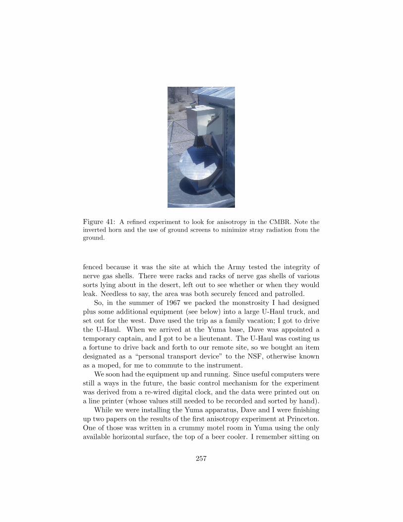
Figure 41: A refined experiment to look for anisotropy in the CMBR. Note theinverted horn and the use of ground screens to minimize stray radiation from theground.

fenced because it was the site at which the Army tested the integrity ofnerve gas shells. There were racks and racks of nerve gas shells of varioussorts lying about in the desert, left out to see whether or when they wouldleak. Needless to say, the area was both securely fenced and patrolled.

So, in the summer of 1967 we packed the monstrosity I had designedplus some additional equipment (see below) into a large U-Haul truck, andset out for the west. Dave used the trip as a family vacation; I got to drivethe U-Haul. When we arrived at the Yuma base, Dave was appointed atemporary captain, and I got to be a lieutenant. The U-Haul was costing usa fortune to drive back and forth to our remote site, so we bought an itemdesignated as a “personal transport device” to the NSF, otherwise knownas a moped, for me to commute to the instrument.

We soon had the equipment up and running. Since useful computers werestill a ways in the future, the basic control mechanism for the experimentwas derived from a re-wired digital clock, and the data were printed out ona line printer (whose values still needed to be recorded and sorted by hand).

While we were installing the Yuma apparatus, Dave and I were finishingup two papers on the results of the first anisotropy experiment at Princeton.One of those was written in a crummy motel room in Yuma using the onlyavailable horizontal surface, the top of a beer cooler. I remember sitting on

257

the dirty green shag carpet, drinking Coors, and the excitement of reachingmilli-K levels in anisotropy.

We also had some time to learn about the nerve gas from soldiers onduty near our site. They explained the use of gas masks — we were issuedwith them in case the nerve gas really did leak — and told us that the firstway to detect leaks of nerve gas was to check out the rabbits. Near eachstack of nerve gas shells there was a hutch containing several standard lab-oratory rabbits. These were placed there since rabbits are highly sensitive,it appears, to nerve gas. So the first alarm for leakages was increased rab-bit mortality. Well, in our brief time in Yuma, the rabbits started to die.There was considerable consternation, not least on our part, until a wiseveterinarian pointed out that all the rabbits had been bought at the sametime, and all of them appeared, entirely naturally, to be reaching the rabbitequivalent of three score and ten. Since we’d escaped the nerve gas, Daveand I joined the soldiers’ favorite game of sitting in a cargo container whilesomeone set o! a military-strength tear gas grenade. The game was to seewho could last the longest before bolting for fresh air. We were young then.

As the Yuma experiment came on line, Dave and Bob Stokes left for thesecond main leg of the summer’s work, a refined, multi-frequency measure-ment of the spectrum of the CMBR. I later joined them, traveling throughthe desert on my trusty “personal transportation device.”

The idea here was to measure the temperature of the CMBR at threedi!erent frequencies — later extended to four by Paul Boynton — using verysimilar apparatus, so that the temperature measurements could be securelyintercompared. In particular, the hope was to show that the spectrum ofthe radiation we were studying is not an exact Rayleigh-Jeans form, withenergy density that varies with frequency & as u! " &2, but instead showssome curvature as the peak of a blackbody spectrum at temperature about3 K is approached.

So we designed radiometers having similar beam sizes, all able to cou-ple to a common calibration cold load. To prevent systematic errors, wedesigned the main horn antenna to look downwards at an angle, making iteasy to couple to a tilted dewar containing the cold load without movingthe apparatus (Fig. 42; Stokes, Partridge and Wilkinson 1967) Thus, to de-flect the beam to the zenith in order to measure the CMBR, we needed touse an oversize reflector. We also arranged the reflector to be movable, sothat the main beam could be cast through di!erent zenith angles, enablingus to measure the atmospheric emission with the same equipment used forthe absolute temperature measurements. The three radiometers used in the1967 campaign are shown in Figure 43; Figure 44 shows the experimental

258

Figure 42: Photo of one of three radiometers used on White Mountain, California,to measure the spectrum of the CMBR (Stokes et al., 1967). The horn antenna iscoupled to a large-diameter cold load.

setup.It is worth mentioning the care we took to avoid systematic error. Dave

Wilkinson, as all who knew him will attest, was extraordinarily careful aboutfinding and eliminating, or at least modeling, sources of systematic error.We took great precautions, for instance, to control emission from the groundleaking into the side lobes of the antennas we used. We were consciousthat emission from the walls of the calibration cold load could present aproblem, and for that reason we expanded the beam and used a large “over-moded” cold load immersed in liquid helium. I have already mentionedquasi-simultaneous measurements of the atmospheric emission. And we alsotook account of the possible emissivity of the reflecting surface.

The result of this work was to produce temperature measurements atthree wavelengths with substantially smaller error bars than previous work-ers had been able to obtain. The error bars were small enough to showrather convincingly that the spectrum of the CMBR does indeed begin toturn over at high frequencies, as expected for a 3 K blackbody (Fig 45). Andthe final temperature we derived from combining observations at the threefrequencies gave a value T = 2.68+0.09

!0.14 K, in remarkably good agreementwith the COBE satellite results that came along nearly two decades later(Stokes, Partridge and Wilkinson 1967; Wilkinson, 1967).

259

Figure 43: The three radiometers used by Bob Stokes, Dave Wilkinson and me tomeasure the CMBR temperature at wavelengths ! = 3.2, 1.6 and 0.96 cm.

The spectral observations were carried out at the highest place in theUnited States with electrical power, the White Mountain Research Stationmaintained by the University of California. Not surprisingly, other groupshad figured out that this was an excellent place from which to observe themicrowave background. When we arrived, we discovered Bernie Burke andhis colleagues busy assembling apparatus that looked an awful lot like thatshown in Figure 43 (Ewing, Burke and Staelin 1967). Our group and hisagreed to work entirely independently, so as not to influence one another’sresults. Yet another group, Welch, Keachie, Thornton and Wrixon (1967),also recognized the value of high altitude observations. However, they en-

Figure 44: A schematic of the radiometers in Figure 43.

260

Figure 45: Results of the Princeton measurements on White Mountain, showinga departure from the Rayleigh-Jeans u! " &2 law.

countered problems with the design of their cold load calibrator, and perhapsas a consequence came up with too low a value for the CMBR temperature.On page 191 Welch describes how that turned out.

Even for these measurements, there was a constant struggle against theatmosphere. Uncertainties in the amount of emission from the atmosphere,particularly from water vapor, dominated the error budget. Throughoutthe experiment, we were worried about possible frequency-dependent sys-tematic errors that could bias our results. I suspect it was at this stage thatDave came to recognize the value of balloon experiments, and even moreof a satellite experiment to get out the atmosphere altogether. Neverthe-less, working with Bob Stokes and Paul Boynton, Dave went on to do onemore ground-based temperature measurement in these years, the measure-ment carried out at 0.33 cm wavelength at the High Altitude Observatoryin the Colorado Rocky Mountains (Boynton, Stokes and Wilkinson 1968).They found T = 2.46+0.40

!0.44 K, which within the errors is consistent with themodern value. And, as a footnote, I went on to join an Italian-Berkeley-Haverford team that returned to White Mountain 15 years later to makerefined spectral measurements at five wavelengths, 0.33 to 12 cm (Smoot etal. 1985).

What were we trying to accomplish with these early experiments? Withthe wisdom of hindsight, it is clear that we were beginning the process ofmining the CMBR for cosmological clues. But in the years 1965-68, the fullvalue of spectral and anisotropy measurements was far from appreciated.

261

The beautiful and influential theoretical work on the power spectrum ofCMBR fluctuations, for instance, lay years in the future. So what were wereally trying to accomplish?

First and foremost, we were trying to establish that the microwave ra-diation detected by Penzias and Wilson (1965) is indeed cosmic, and notcoming from more local sources in the Solar System, the Milky Way, orgalaxies or some other class of extragalactic objects. In the mid-1960’sthere were plenty of skeptics, and numerous noncosmological explanationsof the “excess noise” reported by Penzias and Wilson. We recognized thatstrong proof of cosmic origin lay in two fundamental tests: the blackbodyshape of the spectrum of the radiation and its isotropy on both large andsmall scales.

Electromagnetic radiation pervades the universe. At radio wavelengthsit is dominated by the emission from galaxies and quasars. Could the “ex-cess noise” detected by Penzias and Wilson simply be the high frequencytail of this background? The spectrum holds the key to the answer. Emis-sion from radio galaxies is typically dominated by the synchrotron process,producing a power law spectrum u! " &!" with ' generally in the range0.5 to 1.0. This is very di!erent from a thermal spectrum where u! " &2

at long wavelengths. Another possibility is “free-free” emission from a thinplasma with nonrelativistic electrons, which typically produces a power lawspectrum with ' & 0.1. Such a spectrum, too, is easy to distinguish fromthe truly thermal or blackbody spectrum expected from radiation left overfrom a hot, dense state of the early Universe.

More di"cult to distinguish from a true blackbody spectrum is gray-body — emission fron an optically thin but higher temperature source. Atwavelength ! + 0.3/T cm, with temperature T measured in kelvin, gray-body emission can have the same &2 dependence as true blackbody emission,but the spectrum peaks at shorter wavelengths. To confirm true blackbodyemission at T & 3 K, we needed both to confirm the &2 dependence at longwavelength and find evidence for the peak expected near 0.1 cm wavelength.

It is worth repeating how unlikely it is to find a purely thermal spec-trum in the cosmic setting, where densities tend to be very low. Only if theuniverse were many orders of magnitude denser than it is now could truethermal equilibrium have been established. If the microwave backgroundradiation truly does have a thermal spectrum, it not only establishes thecosmic origin, it shows that the early properties of the Universe were radi-cally di!erent from those prevailing today.

By 1967 we had the answer: we were seeing curvature in the spectrumconsistent with a peak at a wavelength of about 1 mm (Stokes et al., 1967;

262

Wilkinson, 1967).Isotropy is the second test. An observer not moving with respect to

the comoving coordinates of the universe discussed in Chapter 2 (page 14)would see that radiation left over from the big bang appears isotropic (apartfrom the disturbances caused by the departure from a smooth mass distri-bution).26 On the other hand, a Solar System origin would be expectedto produce intensity variations tied to coordinates fixed to the direction tothe Sun. Sources in our galaxy would presumably produce radiation thatpeaks in the direction of the galactic plane, in an anisotropic distributionakin to the concentration of bright stars in the plane of the Milky Way.Such a distribution would introduce a large dipole moment, and particu-larly a quadrupole moment, into the distribution of CMBR intensities. Ifthe radiation were somehow produced by a myriad of extragalactic radiosources, as suggested for instance by Wolfe and Burbidge (1969), it wouldbe “grainy” on a small scale. More precise limits on anisotropy on bothlarge and small scales would, we hoped, kill o! these noncosmological ex-planations. This hope motivated our work, and we soon showed (Partridgeand Wilkinson 1967; Smith and Partridge 1970) that the radiation is indeedhighly isotropic on both large and small angular scales.

Nor were challenges to the cosmic origin of the CMBR mounted solely byinventive theorists. At least one experimental result, the pioneering rocketmeasurement of Shivanadan, Houck and Harwit (1968; see Harwit’s piecehere) seemed to favor a graybody spectrum. The results naturally raiseddoubts about the cosmic origin of the microwave background.

All of these results, attacks on the very notion of the “primeval fireball,”were very much on our minds as we mounted the experiments describedabove and wrote up our results.

One anecdote encapsulates the skeptical air of the times. In 1969, as Irecall, I gave a talk on our Yuma experiment at a meeting at Caltech. In thequestion period a formally dressed, middle-aged man in the back asked, ine!ect, “Given that you see no change in emission as the sky passes overheadeach day, how do you know your equipment is even switched on?” Fortu-nately — since the questioner was Charles Townes — I gave an appropriateanswer, describing in detail the care we took to calibrate the instrument.

So I would say that in the 1960s, we were on a mission to convince theskeptics, an attitude that strongly colors an early review of the primeval

26Parenthetically, this would not be the case if the universe itself were expanding in ananisotropic way. Ellis (page 288) notes that this idea was of considerable interest in the1960s.

263

fireball published in the spring 1969 issue of the American Scientist (Par-tridge 1969). I would suggest, however, that there was another influenceat work. We were, after all, working for Bob Dicke, acknowledged as themaster of the beautiful null experiment. These are experiments designed toto test the absence of some physical e!ect by establishing more and morestringent upper limits on the magnitude of the e!ect. Dicke’s ultrasensitiveversion of the Etvos experiment, for instance, showed that there are no dif-ferences in the way gravity acts on di!erent chemical elements to a level ofroughly one part in 1011. I will speak only for myself here, but part of themotivation driving me was to do better and better null experiments on theCMBR, in particular to establish lower and lower upper limits on possiblefluctuations in the CMBR (see Partridge 2004). In other words, I am con-fessing to having been driven less by theoretical concerns or predictions thanby an experimenter’s lust to do the best possible experiment, and to coveras much parameter space — in this case sensitivity and angular scale — aspossible. As Dave and I were planning better experiments to push downlimits on the amplitude of the temperature fluctuations on degree scales, Iwas also thinking about ways to limit anisotropies on small angular scales.This required the use of larger aperture devices, since the angular scale goesapproximately inversely as the diameter. Others — Ned Conklin (1967),Eugene Epstein (1967) and Penzias, Schraml and Wilson (1969) — had al-ready set upper limits on arcminute-scale fluctuations; Paul Boynton and Irealized we could reach both smaller angular scales and higher sensitivityusing a 36-foot telescope operated by the National Radio Astronomy Obser-vatory. Our results turned out to be only mildly interesting, and I mentionthem simply because they reflect at least one person’s motivation in theseearly years — to set the best possible limits on fluctuations at all angularscales.

That I was not alone in this aim is reflected in the way in which anisotropymeasurements were presented in these early years, and for at least a decadeafterwards (see Fig. 46). What is shown is basically a plot of upper limits onthe fractional temperature fluctuations )T/T across the sky, with little refer-ence to any underlying theory of what the angular spectrum of anisotropiesmight be (though we did know that the overall amplitude would be a!ectedby the mass density fluctuations). Also reflecting the focus on upper limitsis the fact that a paper I wrote with Italian colleagues in the early 1980s wasinitially rejected solely on the grounds that the upper limit we establishedwas not as low as the upper limit somebody else had established, despitethe fact that we were working at degree angular scales and the “better”experiment was at arcminute scales.

264

Figure 46: An early (and poor) way of representing upper limits on anisotropy inthe CMBR on various angular scales.

Figure 47: The number of CMBR-related papers published each year. Note thelack of activity in the years 1969-77.

Is it possible that the drive to set lower and lower limits on CMBRanisotropies has a contemporary analogue in the drive to determine the cos-mic equation of state parameter w that is supposed to describe the evolutionof the dark energy density? Does the (expensive) e!ort to improve limits onthis e!ect parallel our e!orts 40 years ago to improve limits on the CMBRtemperature anisotropy? Indeed, the same question could be asked aboutplans to measure another cosmic parameter, the ratio, r, of tensor to scalaranisotropy perturbations. Clever scientists are designing better and bettermethods of refining measurements of r and w, but without much theoreticalguidance (especially on r).

Finally, I would like to explore a phase change that occurred in the field

265

in the early 1970s. It may surprise some of you, who see the CMBR as agiant growth industry, to learn that by the end of the 1960s interest in it waswaning, or at least changing. That is reflected in the rate of publication ofpapers dealing with the CMBR shown in Figure 47, taken from the “history”chapter in my book, 3K (Partridge 1995). Before exploring some reasonsfor temporary dwindling interest in the CMBR, let me make a much morepositive point: this is the time when many other groups here, in Europe andin Russia began to take an interest in improved CMBR experiments.

The emergence and success of these groups is linked to one of the reasonsI see for the cooling of ardor at Princeton. By the late 1960s we had, ine!ect, done all the easy experiments. The experiments Dave and I did were,as I liked to say, “one-Cadillac scale,” costing of the order of $10 to 20,000each. They were constructed almost entirely from commercially availablecomponents. To improve these experiments, new detectors and optics wereneeded, as were instruments designed specifically for the detection of CMBRanisotropies or the precision measurement of the CMBR spectrum. In addi-tion to new technology, better observing strategies were needed (recall myremarks above on problems created by the atmosphere). The same stric-tures applied to the use of existing radio telescopes: observers had pushedthem to their technological limits as well.

New groups brought new techniques and new technologies to bear. Iwant to mention specifically the introduction of bolometric detectors into thefield, and to praise the foresight of people like Paul Richards and FrancescoMelchiorri, and of Rai Weiss, who has written for this volume. Francescowas a pioneer in the field, who unfortunately passed away in 2005.

So there was a pause while new technologies and techniques were broughtto bear. Along with new groups joining the field, Dave Wilkinson wiselymoved in the direction of balloon experiments. I got interested in the useof radio-frequency interferometry to probe yet smaller angular scales. Theintroduction or exploration of these new techniques took time, and that isin part responsible for the drop in activity in the CMBR field in the early1970s.

Another factor, at least in the case of Princeton’s Gravity Group, wasthe explosion of other interesting things to do in astrophysics, ranging frompulsar timing to searches for “primeval galaxies.” The experimentalists of theGravity Group found lots of other intriguing things to do while we waitedto sort out new CMBR technologies and techniques. Dave, for instance,began to explore limits on extragalactic optical backgrounds and oversawMarc Davis’s pioneering search for primeval galaxies. I mounted a separatesearch for primeval galaxies, and got interested in observational tests of the

266

Wheeler-Feynman (1945) absorber theory (Partridge 1973) and searches forbursts of radio-frequency emission. Both Dave and I, joined by Ed Grothand Paul Boynton, spent a lot of time from the spring of 1969 on makingprecision timing measurements of the optical pulses of the Crab NebulaPulsar. In an ironic twist, we felt we had discovered evidence that the CrabNebula pulsar is slowing down due to the loss of energy by gravitationalradiation; it turned out that Nature had thrown us a curve ball in the formof a glitch in the pulsar period. But another, cleaner pulsar system wouldreveal energy loss by gravitational radiation and win the Nobel Prize forRussell Hulse and Joe Taylor.

I will end by floating an idea that may be strongly colored by retrospec-tive wisdom. Could the lull in CMBR activities have been in part influencedby the fact that we were beginning to pay some attention to theoreticalpredictions as to the properties of CMBR anisotropies and spectral distor-tions? That is, instead of blindly trying to set better and better limits onboth anisotropy and spectral distortion at a range of wavelengths and scales,were we, I wonder, beginning to recognize (a) how hard it would be to seemeaningful spectral distortions and (b) that the amplitude of anisotropieswould in general be very small except on certain angular scales? Frankly,my recollection of my mood in the late 1960s and early 1970s is now a littletoo hazy for me to say for sure. What I can say is that the five years, 1965to 70, were not only the years that truly established physical cosmology, butwere a hell of a lot of fun!

267

Ronald N. Bracewell and Edward K. Conklin: Early Cosmic Back-ground Studies at Stanford Radio Astronomy Institute

Ron Bracewell has been at Stanford since 1955 and is now professor emer-itus. Ned Conklin was a graduate student at Stanford at the time describedhere. After a number of years at NRAO and Arecibo, he co-founded FORTH,Inc. and worked in the field of scientific computer programming until retiringrecently.

When the existence of the CMBR was announced in 1965, we discussedvarious kinds of measurements that might be made. Ned had been lookingfor a thesis topic, and this was an interesting and brand new field. Themost obvious measurement was the absolute amplitude at one or more newwavelengths, but that would have been an extremely di"cult experiment.It’s relatively easy to make a measurement of the apparent temperature rel-ative to that of a known absorber when an antenna is pointed at empty sky,but that’s only the start. Then all the other possible sources of antennatemperature such as atmospheric losses, losses in the system and the an-tenna, unwanted pickup in the sidelobes, etc. must be accurately estimatedor measured and subtracted from the observation to yield the residual (ifany) due to the CMBR itself. In nearly all cases these unwanted sources ofradiation are substantially higher than the few degrees of the CMBR, andso the subtraction process is prone to errors. Further, we recognized that,once a measurement had been published at one frequency and a thermalspectrum was posited, there would be the unconscious bias towards con-firming it at other frequencies, leading to a situation where one might thinkof extraneous radiation sources contributing to a measured value, subtracttheir e!ect until the CMBR temperature was reached and then stop lookingquite as diligently, so that a secondary measurement would not be trulyindependent.

Discarding the absolute value left measurements of the angular structure(if any) of the radiation field. In their original paper Penzias and Wilson(1965) reported that the CMBR was isotropic, but the precision of their mea-surements was low. Two possibilities presented themselves (Bracewell 1966;Conklin 1966), each with its own set of experimental problems – measuringthe fine scale on the order of arc-minutes (inhomogeneity), and measuringthe large scale on the order of degrees (anisotropy). In the end we pursuedboth.

The weak cosmic background radiation detected by Penzias and Wil-son was reported as isotropic. So it was with cosmic rays, but they werequickly found to vary with altitude, latitude, and season, so we thought

268

it likely that the cosmic background also might prove to be not isotropic.Any anisotropy of the remote cosmic background would be hard to ad-dress but in the summer of 1967, when these measurements were under-taken, Stanford Radio Astronomy Institute was by chance well equippedto look for inhomogeneity in the newly announced microwave radiation. A735-foot minimum-redundancy microwave array of five interconnected 60-foot paraboloids and associated electronics was already under construction(Bracewell et al. 1973). With particular attention to symmetry and match-ing at a frequency of 10,690 MHz, a pair of identical feed horns was installedat the focus of one 60-foot dish, one horn pointing to the zenith, the otherdown on the level paraboloid. The paraboloid was tilted very slightly o!zenith so as to cause the radio source Cygnus A to pass through the centerof the fixed antenna beam and serve as a calibration source.

A waveguide tee junction, built to connect the two horns, incorporated atwo-state ferrite circulator; in one state the signal received from the radiome-ter was that from the upward-looking horn whose beamwidth was about 80",and in the other state the signal was from the horn that fed the paraboloidforming a resultant beamwidth of about 13$. The circulator was subjectedto square-wave switching at 37 Hz. The signal delivered to the output armof the tee, after preamplification, mixing, intermediate frequency amplifica-tion, and detection thus consisted of a noisy square wave jumping betweenthe antenna temperatures in the 80" beam and the 13$ beam formed by theparaboloid. One can understand that in the state of electronics of the dayextreme care was needed to deal quantitatively with such a small jump.

The response to the upward-pointing horn was expected to be 900 K(the noise temperature of the radiometer) plus the mean intensity of thecosmic background, now known to be approximately 2.7K, plus a few moredegrees from any atmospheric radiation and ground radiation in the antennasidelobes. The response of the horn looking into the reflector and focusedinto a pencil beam 13$ wide would be nearly the same and the di!erencewould reveal any local departure from isotropy as the sky rotated overhead.Clearly, constancy with time of the 900K noise temperature of the receiveris also of the essence of the experimental design, as well as constancy of theatmospheric radiation.

The experimental di!erential results did show both a long-term trend(over a period of hours) which was evidently caused by thermal e!ects inthe radiometer and switched circulator, and short-term fluctuations whichdid not repeat from day to day and which correlated fairly well with changingatmospheric conditions. The long-term trend was removed by subtracting ahalf-hour running average from the data; the e!ect of this was to limit the

269

inhomogeneity analysis to beamwidths less than about 7.5" (30 m. of rightascension), not a serious limitation. The short-term atmospheric fluctua-tions, being random, could not be removed and simply added to the e!ectiver.m.s. antenna temperature. Out of 65 days of observation, the data from29 days were rejected entirely as having excessive short-term fluctuations,and the remaining 36 days of data were averaged and analyzed.

The results did not show any noticeable inhomogeneities in a strip of skylocated at 40.6" N declination and from 11 to 19 h of right ascension. Themean observed r.m.s. antenna temperature of the data, although somewhathigher than expected, decreased as N!1/2 up to the limits of our data, whereN was the number of days in the average, indicating that the results werepurely statistical and that no floor of intrinsic CMBR inhomogeneity waslimiting the observed results. At the 13$ beamwidth of the paraboloid, the 3*limit to any intrinsic inhomogeneities in our data was about 7.9 millikelvins.By integration of the data, even lower limits could be set for larger angularscales & up to a few degrees, and limits could also be set for angular scalessmaller than 13$, recognizing that their amplitudes had been reduced by thespatial smoothing in the antenna beam. The final published results were* = 103/& for 0$ < & < 13$, and * = 28&!1/2 for 13$ < & < 120$, where *is the r.m.s. intrinsic inhomogeneity in millikelvins (Conklin and Bracewell1967). These limits were low enough to be useful constraints on variouscompeting theories of the CMBR.

The very-low-noise radiometers widely available today were not commonin the late 1960’s and since statistical r.m.s. fluctuations unfortunatelydecrease only as the square root of the integration time, improving theinhomogeneity limits below the values quoted above would have requiredexcessive observing time. Also, the borrowed equipment being used for theexperiment was needed for the completion of the five-element array, so atthis point we turned our attention to the anisotropy question. Here we hadat least one likely positive result on theoretical grounds, albeit at a very lowlevel. If the Earth were moving with respect to the rest frame of the CMBR,then there would be an increase in the CMBR temperature in the directionof motion, and a similar decrease in the opposite direction. (The theoryis discussed below.) A speed of 300 km s!1 would result in a temperaturechange of only one part in a thousand, or about 2.7 millikelvins, quite anexperimental challenge in that era (and still not easy).

Measuring this kind of e!ect with any type of moving or scanning an-tenna was obviously out of the question. Varying ground pick-up in antennasidelobes and changes in atmospheric re-radiation would far outswamp thefew millikelvins from the CMBR itself. The only hope was to construct some

270

Figure 48: Historic horns through which flowed the radiant energy (estimated atroughly half an erg during the integration time of 425 hours) that revealed theSun’s motion through the cosmos.

kind of system that was fixed with respect to the ground and let the skysweep through the beam. The dipole anisotropy would then appear in theantenna temperature as a sine wave with an amplitude proportional to thevelocity and a period of one sidereal day.

The apex of the Earth’s motion (if any) with respect to the CMBRwas completely unknown. But unless it were closely aligned with the northcelestial pole, there would be an equatorial component which could be mea-sured most easily. As with the inhomogeneity experiment, a radiometerwould need to be switching between two sources with antenna tempera-tures as nearly equal as we could devise, and yet be sensitive to the dipoleanisotropy. Because of the extremely low amplitude, it was desirable thatno integration time be spent on reference loads or reference patches of skysuch as the north celestial pole.

We ended up with an antenna system consisting of two identical horns(Fig. 48) with 14" beamwidths directed east and west respectively at a zenithangle of 30" and enclosed in a truncated conical screen to intercept radia-tion from the ground. To limit reception of unwanted thermal radiation fromthe surroundings these horns incorporated, at their rims, the short-circuitedquarter-wave transmission line chokes familiar from microwave radar prac-tice.

As the sky passed overhead any temperature di!erence between the two

271

patches of sky pointed at would contribute a component to the recordedsystem temperature. As the earth rotates a given region of sky will pass firstthrough the eastern antenna beam and then, several hours later, throughthe western beam. Since the polarity of the antenna temperature is oppositefor the two antennas, this configuration is measuring the finite di!erence ofthe temperature distribution in the sky. It can be shown that the originalsky distribution is recoverable from the finite di!erence record except forthe mean value, which is not of interest here. The amplitude of any dipoleanisotropy is reduced somewhat by the finite di!erencing, but the sensitivityremains higher than for a fixed reference system.

An extremely sensitive and stable radiometer was essential for this ex-periment. Receivers with very low system temperatures (such as masers)were just not in the budget, as well as being di"cult to keep stable. Sincethe CMBR is essentially an extremely wide bandwidth thermal signal, analternative for increasing the sensitivity was to increase the bandwidth ofthe receiver. We were fortunate in obtaining a very wide bandwidth, fairlylow noise tunnel diode amplifier on loan from NASA, and the radiometersystem was built around it. The wide bandwidth made the radiometer sus-ceptible to airborne radar, but that was sporadic, and easily detected on achart recorder and eliminated from the data.

The noise figure of the tunnel diode amplifier was such that it was the-oretically capable of reaching an r.m.s. output fluctuation of 5 millikelvinsfor a one-minute average. It took months of patient experimentation to con-struct a complete radiometer system that would stably operate at that level,but eventually we succeeded. A key feature that was added at this time wasthat the entire radiometer including the antennas and front-end electronicswas mounted on a turntable. At five minute intervals the turntable rotated180", interchanging the east and west antennas. This second di!erencingremoved the last small asymmetries and drifts in the electronics and left uswith a system that appeared capable of detecting millikelvin variations inthe CMBR.

Just a few days of observation near sea level at Stanford were enough toshow that operation there was hopeless because of fluctuating atmosphericabsorption and re-radiation at the 8 GHz frequency of our system. Weneeded an observing site with extremely low water vapor, and that meant ingeneral high altitude and ambient temperatures below zero degrees C. Againwe were fortunate in finding a reasonably accessible high-altitude facility atthe University of California’s White Mountain Research Station. The entireradiometer and associated data-taking electronics were installed in a smalltrailer and towed up to the Barcroft station at latitude 37" N in October

272

1968. Here, at an altitude of 12,500 feet and atmospheric pressure less thantwo-thirds of that at sea level, the receiver performed acceptably close to itstheoretical limit (although the human observer had di"culties!).

Because of solar radiation in the antenna sidelobes, useful data couldonly be taken at night time. Two month-long observations were made inOctober 1968 and April 1969 and were combined to obtain a complete 24-hour record. It was immediately evident that non-thermal galactic radiationwas a!ecting the data; this was removed by extrapolating an all-sky mapof the galactic antenna temperature to our 8 GHz observing frequency andsubtracting it.

Details of the reduction procedure are given by Conklin (1969), alongwith a preliminary result based on the first observing run. The final reportedresult for the first detection of the dipole asymmetry was an amplitude of2.28 mK (formal standard error ±0.68 mK, total estimated error ±0.92 mK)at a phase corresponding to right ascension 10 h 58 m (Conklin 1972), in-dicating a solar velocity in the equatorial plane of 255 ± 76 (formal), ±103(total) km s!1. No significant smaller-scale anisotropies were seen in thedata, which covered a region of sky from about 25" to 39" N declinationand the full range of right ascension. The precision achieved in the lightof determinations years later with much improved electronics, was quiterespectable.

The theoretical impact of the discovery that the Sun possessed an abso-lute motion through the Universe was striking, both to the scientific commu-nity and to science writers (Sullivan, 1969) addressing the general public.When the letter appeared in Nature a letter to Bracewell from ProfessorJakob L. Salpeter in Adelaide reported on a paper written by Kurd vonMosengeil (1907) where we read:

Alle Versuche, einen einfluß der Erdgeschwindigkeit auf die elek-trodynamischen Erscheinungen festzustellen, haben ein negativesResultat ergeben. Um dies zu erklaren, haben H.A. Lorentz1)und in noch allgemeinerer Fassung A. Einstein2) das ,,Prinzip derRelativitat“ eingefuhrt, nach welchem es prinzipiell unmoglichist, einen derartigen Einfluß aufzufinden.

All attempts to establish an influence of Earth’s velocity on electrody-namic phenomena have given a negative result. To explain this H.A.Lorentz (1904), and in greater generality A. Einstein (1905), have in-troduced the principle of relativity, according to which it is in principleimpossible to discover such an influence.

273

We now know more about special relativity. In 1996 textbooks of ther-modynamics did not mention moving observers; one could only wonder whatappearance the microwave sky would present. The two reports (Bracewell1968) deduced that the brightness observed in the forward direction wouldincrease and that the spectral distribution would still be that of a blackbody, but with a temperature apparently higher than that seen by a sta-tionary observer. Naturally the spectral components would be shifted tohigher frequencies by Doppler e!ect, but that alone would not result in aPlanck spectrum; two other e!ects are involved. Stellar aberration wouldreduce the solid angles subtended by sky elements on or near the apex of so-lar motion and this would result in an increase in brightness as measured inwatts per square meter per hertz per steradian. Finally, the electromagneticfield strengths of both the electric and magnetic fields would be increaseda little by the relativistic Lorentz transformation. Combining these threee!ects we found (Bracewell and Conklin 1967) that the spectrum wouldpreserve Planck’s blackbody form. In the forward direction, if the observerwas moving at one thousandth of the light velocity c, the apparent tem-perature would be greater by one-thousandth than the temperature T seenby an observer at rest. For an observer moving with velocity v we foundthat, in a direction making an angle , with the direction of motion, theobserved temperature would be T [1 + (v/c) cos ,]. If the observer’s velocitywas not negligible with respect to c then the observed temperature wouldbe T [1 + $ cos ,/

!1! $2], where $ = v/c.

Though a literature search did not uncover this result it was reason-able to assume that it was known; the internal reports (Glints) were forthe edification of the graduate students. It was therefore a surprise whenCondon and Harwit (1968) reported that the spectrum seen by a movingobserver would not be that of a black-body. The internal memorandum wasdusted o! and submitted for publication to the appropriate journal but,being rejected, was resubmitted to Nature (Bracewell and Conklin, 1968).Shortly after that we learned from Prof. Salpeter’s letter, that the same con-clusion had been reached by von Mosengeil in 1907. Our discovery of theLorentz/Einstein undiscoverable naturally made a wide impression. In duecourse Corey and Wilkinson (1976) of Princeton University launched manyballoon flights and extended Conklin’s results to a range of declinations,and Smoot, Gorenstein, and Muller (1977) of the University of California atBerkeley made many flights with the Kuiper flying observatory stationed atNASA Ames Laboratory in Mountain View, California. These more detailedendeavors neatly bracketed the original Stanford discovery (Fig. 49). Theremarkable detail discernible in the Cosmic Background Explorer satellite

274

Figure 49: Constellation chart showing a naked-eye observer on the bridge ofSpaceship Sun that we are heading toward the point labeled “Apex.” The coor-dinates have been refined by spacecraft observations. Also shown are the earliestreports from Stanford, Princeton, and Berkeley.

images of later years have continued to grip the lay imagination.The Sun’s motion might reveal itself in other ways, for example it should

be evidenced by a dependence of density of distant galaxies on ,; they shouldbe less tightly packed in the general direction of Pisces than in the directionof Sextans. Counts of faint galaxies in the zones , < 15" and 165" < , < 180"

should di!er by about a part in a thousand.Meanwhile, the e!ort to discern a dipole component against a spatial

noise background had left open the question whether spatial fluctuationsexisted, on a fine angular scale, in the background radiation. Careful obser-vation did not reveal any such pattern but did allow an upper limit to beplaced on the size of any such departures, as averaged over small solid an-gles. A technically remarkable low limit of 0.005K for beamwidths broaderthan 10 arcminutes was reported (Bracewell and Conklin 1967).

This was less than exciting for an aspiring Ph.D. candidate but caughtthe attention of theoretical cosmologists and was quoted for several years asa constraint on assorted cosmological theories.

275

Thus in these early days, three significant contributions were made tothe future and continuing studies of the fundamentally significant cosmicbackground radiation.

When the National Science Foundation withdrew support from univer-sities in order to fund the National Radio Astronomy Observatory the sta!of the Stanford Radio Astronomy Institute dispersed, some to NRAO, someto radio astronomy elsewhere, and some to industry. The remaining grad-uate students eked out their dissertations with funding support for medicalimaging, solar thermovoltaic energy, theory of dynamic spectra, etc. Themothballed observatory was torn down on March 11, 2006.

Postscript: On Being the First to Know (EKC). In the summer of 69 I wasreducing all the data that had been taken in our two month-long observingruns looking for CMBR anisotropy. This involved hundreds of IBM cardsfilled with five-digit numbers, each one indicating the value of a one-minuteintegration from the radiometer, and a complex program that combined theobserving runs, aligned and averaged the data, subtracted the estimatedgalactic radiation and Fourier-transformed the result. Because the ampli-tude of the dipole component was expected to be very small, there was noway to get a preliminary indication along the way of any statistically signif-icant result; it was all or nothing. Late one evening I was at the ComputerCenter, ready at last with the run that would have the final result. I sub-mitted the deck of cards to the mainframe computer operator, and in abouthalf an hour, back came the stack of output paper. This would have twoimportant numbers in it that represented about 18 months of e!ort: thedipole anisotropy and its standard error. Did I have something significant?Yes!

At that point I recalled an article I had read recently, I believe by PhilipMorrison, that one of the joys of research like this is that for a moment,until you choose to tell someone else, there is something you know that noone else in the world knows. I went home that night elated to have had thathappen to me, and although all of this occurred over 35 years ago I havenever forgotten it.

276

Stephen Boughn: The Early Days of the CMBR: An Undergrad-uate’s Perspective

Steve Boughn is professor of physics and astronomy at Haverford College.His expertise includes the theory and detection of gravitational waves, extra-galactic astronomy and cosmology.

I’m not sure why Peebles and Partridge invited me to participate in thiscollection of remembrances since I was only an undergraduate in the 1960’sand most of what was swirling around above my head was just that, overmy head. Of course, I’ve learned a great deal about Big Bang cosmologyand the CMBR since then, and I have been involved in CMBR research o!and on for the last 40 years. However, I’ll endeavor to relate as accuratelyas possible what was going on in my mind back then in the hope that therecollections of a novice might be of some interest or at least provide someamusement.

I enrolled as an undergraduate at Princeton University in 1965, the sameyear as the announcement of the discovery of the CMBR. I had been en-ticed by special relativity early in high school and so arrived at Princetoncommitted to becoming a physics major. Astronomy had also been a sourceof fascination for me since I was very young. It was an exciting time in as-tronomy; quasars had just been discovered and pulsars were soon to follow.However, my entire knowledge of cosmology consisted of Hubble’s discov-ery of the expansion of the Universe and the notion that Einstein’s theorywas capable of “explaining” what was going on. Still that was what excitedme most. Even so, for my first three years at Princeton I busied myselfstudying physics (no astronomy - even though today I’m a professor of as-tronomy, I’ve never actually taken a course in astronomy!). Then in 1968,at the end of my junior year, it was time to choose a senior thesis topic. Ofcourse, I immediately pestered the people in Dicke’s Gravity Group for pos-sible projects. I still remember the suggestions. Dicke suggested a projecthaving to do with solar oblateness and its relation to Brans-Dicke theory.John Wheeler suggested two projects, one having to do with the draggingof inertial frames (at Stanford, Francis Everett and my future PhD advisorBill Fairbank were already deeply involved in what is now known as GravityProbe B to test this e!ect). Wheeler knew I was from Wyoming and sodescribed this to me in terms of a cowboy’s lariat. The second project hesuggested was experimental. He thought it would be interesting to try tomeasure the advanced potential implied by the Feynman-Wheeler absorbertheory of radiation using one of the CMBR radiometers of Dave Wilkinson

277

and Bruce Partridge. Partridge and Wilkinson suggested a project also in-volving one of their microwave radiometers, but used in a more standard wayto attempt to measure the dipole and quadrupole moments of the CMBR.This is what I chose and that decision had a lasting impact on my profes-sional career. I hope I realized at the time how fortunate I was to have thechoice (as an undergraduate) to work with such wonderful scientists, but Iprobably didn’t.

I began reading about the CMBR right away but didn’t know aboutgeneral relativity or about cosmological models expect for very qualitativedescriptions. So for me, my isotropy project soon became more a matterof getting the apparatus to work and to make a reliable measurement thanof thinking about the cosmological consequences. I’m sure that others willmake this same point, that is, that while the motivation of an experimentis extremely important, getting the experiment to work and making thebest possible measurement usually takes over and determines the measureof success — at least in one’s own mind. If this weren’t the case, I suspectthat experiments would not be as successful as they are nor would scienceadvance as rapidly as it does. I do remember being extremely careful totrack down all the possible sources of systematic error, something I’m sure Iacquired from Partridge and Wilkinson, and that has held me in good steadas an experimentalist.

The instrument was an 8.6-mm radiometer used by Dave to measure theCMBR spectrum and the plan was to compare the temperature of two pointsin the sky separated by 90" on the celestial equator. The 90" separation waspicked to maximize the sensitivity to a quadrupole signal in the CMBR — Ibelieve that one motivation was a possible anisotropic expansion of the uni-verse, but to an undergraduate these were just words. The real motivationwas to do an isotropy experiment at a shorter wavelength than other experi-ments to see if the previously measured CMBR isotropy was independent ofwavelength. At the time, extragalactic sources for the CMBR had not beencompletely ruled out and one might expect that these sources would exhibitanisotropy at higher frequencies. I’m sure some Big Bang enthusiasts mightsay we were wasting our time; however, such null tests are all part of theimportant “network of measurements” that validate any scientific model. Itnow seems hard to believe that the data were recorded on many, many rollsof Esterline-Angus, pen and ink, strip chart paper that were painstakinglyanalyzed by hand. Of course, we found no anisotropy at our level of sensi-tivity, about 0.4 percent, a respectable limit but certainly not the best atthe time. The design of the size and shape of the reflector was left entirelyup to me. Since the beam was required to switch by 90" on the sky, the

278

reflector should be switched by ±22.5", or so I thought. That would onlybe true if the beams were reflected in a direction perpendicular to the axisof the reflector. They were not. As a result the beam throw on the sky was64", a value that prompted several inquiries after our paper was published(Boughn, Fram & Patridge 1971). It was a both an embarrassing lessonfor me and a testament to the involvement that Partridge and Wilkinsonexpected from their undergraduate students.

I assembled the radiometer in the Gravity Group haunt, a large areain the northwest corner of the basement of Palmer Laboratory, the homeof the Physics Department. The place was an absolute maze with endlesspiles of equipment punctuated by several desks supporting stacks of papersthat often spilled onto the floor. One evening I brought my two month olddaughter with me while I worked on the radiometer. I tucked her in hercarrier in a safe place among the jumble of apparatus as I worked on theradiometer. Some time later Dicke wandered in to search for something anduttered, “Well, what have we here!” as he happened, with delightful surprise,upon my daughter. During the day the place was a beehive of activity withthree other undergraduates (Mike Smith, David Payne, and Bill Baron)working on CMBR related projects, one of which was the first attempt tomeasure the polarization of the CMBR; two senior graduate students (PaulHenry and Karl Davis), who were building more radiometers, one of whichwas to be the first balloon-borne instrument; three more junior graduatestudents (Ed Groth, Jim Cambell, and Dave Fram), who had just arrivedat Princeton; three postdocs (Jer Yu, Paul Boynton, and Neil Rasband),who were also working on the CMBR; and our leaders, Dicke, Wilkinson,Peebles, and Partridge. The excitement was palpable and the communityspirit of the quest ever present as everyone helped with each other’s projects.It was no wonder that I had a somewhat inflated notion of the importanceto physics of what was going on there.

By the time I left Princeton in the spring of 1969, I was finally beginningto learn a little general relativity and began to think a little more deeplyabout the CMBR. After reading some of the fundamental papers on grav-itational lensing I began to wonder if perhaps gravitational lensing of theCMBR by massive galaxies might not result in some anisotropy. I don’tknow if I mentioned this to Wilkinson or Partridge, but if I did I suspectthey would have told me (with a smile) to go away and think about it somemore. I did and after a laborious calculation was surprised that everythingcanceled out and lensing could not, in fact, generate any anisotropy what-soever. It seems there is something called the ”brightness theorem” that isvalid even in the presence of gravity. Even though I was beginning to think

279

more deeply I was, alas, still a novice. It turns out that collapsing or ex-panding concentrations of mass can generate anisotropies in the CMBR viathe gravitational redshift, as was predicted by Sachs and Wolfe (1967), butit wasn’t until 3 years ago that I and others detected this “integrated Sachs-Wolfe e!ect” and found its amplitude to be consistent with the existence ofa cosmological constant, another thread in the “network of measurements”.

I was involved in two more rounds of anisotropy experiments, one in thelate 1970s and the other in the late 1980s. These took place well after thedecade that is the subject of this book; however, I think there is an impor-tant point regarding these and other null CMBR anisotropy measurementsof that 25 year period. It’s understandable that the measure of success of agiven measurement was, in part, determined by the upper limit it set on thelevel of the fluctuations in the CMBR. However, it seemed that some people(usually theorists) in the field took these limits very seriously, distinguishingbetween experiments that yielded upper limits that di!ered by as little as20 or 30 percent. Most experimentalists realize that di!erentiating obser-vations on this basis is nonsense. I once conferred with a statistician aboutthe best and most robust statistic that I should use to set an upper limitto CMBR fluctuations. He seemed mystified by my use of statistics andresponded that what I should properly do is to report the sensitivity of myinstrument and then say whether or not I detected anything. Setting upperlimits, he maintained, is not a proper use of statistics. Hmmm.... I onceasked Wilkinson about what I described as over-interpreting the statistics ofnull results. He said not to worry. This situation was just the result of anx-ious cosmologists biding their time until CMBR fluctuations were actuallyobserved. Sure enough, this came to pass. However, I do see a hint of thesame problem returning, with some people judging cosmological observa-tions by their usefulness in reducing the errors on the various parameters ofthe currently favored cosmological model and paying scant attention to thediversity of those observations, a diversity that will be absolutely necessaryin ushering in any new understanding of our universe.

I know now that cosmology certainly wasn’t considered to be one ofthe important areas of physics research in the 1960s and I was well awarethen that there were other great discoveries being made. The professor ofmy very first physics course at Princeton was Val Fitch, who had the yearbefore discovered CP violation in particle physics, a discovery for which heand Jim Cronin would later receive the Nobel Prize. (The second semesterof the course was taught by M.L. Goldberger, another notable figure inparticle physics and future President of Caltech.) Yet, from my limited

280

point of view (in the biased environment of Princeton’s Gravity Group) Iperceived cosmology as one of the most important and fascinating areas ofall fundamental science. I still do.

281

Paul S. Henry: A Graduate Student’s Perspective

Paul Henry is a Member of the Technical Sta! of AT&T Laboratories. Histhesis experience at Princeton sparked a lifelong career in telecommunica-tions research, which continues to this day.

The last thing I remember from that day is Dusty Rhoads and Gene DeFreecedepositing me at my motel room. Dave Wilkinson, my thesis advisor, waswaiting for me and was none too happy. Where in hell have you been? hedemanded. I’ve been looking all over for you. We have an interview withthe Hobbs paper in half an hour.

Not now, Dave, please. You can cover for me. And at that point Ipassed out.

So that’s what it had come to. After four years of grad school — most ofthem spent laboring in Bob Dicke’s Gravity Research Group (the “GRG”),preparing for what was supposed to be a definitive experiment in observa-tional cosmology — I had ended up in a Hobbs, New Mexico motel, tankedto the gills with 190-proof Everclear grain alcohol.

The trouble had begun about two years earlier, when Dave and PaulBoynton (a postdoc in Dicke’s group) recognized that ground-based mea-surements of the isotropy of the CMBR would forever be plagued by atmo-spheric e!ects, especially emissions due to water vapor. High altitude wasthe key to success. After rejecting satellite- and aircraft-based platforms,they concluded that a balloon-borne experiment, flying above 99% of thewater vapor in the Earth’s atmosphere, could be a cost-e!ective approach.A low-noise, wideband radiometer, slowly rotating to scan the sky, couldcollect enough data in a 10-hour flight to yield a good estimate of the 24-hour (dipole) anisotropy of the CMBR. (Ned Conklin and Ron Bracewellat Stanford University had already done a lovely experiment to measurethe equatorial component of the anisotropy [Conklin 1969], but the polarcomponent, and therefore the total magnitude, was still unknown.) No onein the GRG had ever worked with research balloons before, but Dave haddiscovered that a federal agency, the National Center for Atmospheric Re-search (NCAR), could provide the equipment and services needed to conducthigh-altitude research experiments. He asked me to dig a bit deeper.

I had come to Princeton solely because a college professor had men-tioned Dicke’s work in cosmology as proof that you didn’t need to be in thethen-fashionable mainstream of big-time, high-energy physics in order to doexciting research. Believing then, as I do now, that less is more, this com-ment sounded like high praise to me. I had zero knowledge of cosmology(Who’s Hubble?); it was the possibility of doing small-scale experimental

282

physics, not cosmology per se, that excited me. The experiment proposedby Dave and Paul was just what I had been looking for.

The next thing I knew, I was up to my eyeballs in the details of microwaveradiometers, thermal design, telemetry, and failure-mode analysis. Dave andPaul apparently trusted me to manage the project on my own, or suspectedthat it was going to be a huge sink of time they’d rather not invest. Eitherway, they gave me more than enough rope to hang myself.

As I labored through the endless details of design, construction andtesting of my equipment, I began to sense that my little project, thoughextremely modest by the usual standards of experimental physics, was partof a much bigger picture, a brewing revolution in cosmology. Time and again,I’d overhear the big shots of the GRG (to me, anyone with a PhD qualified asa big shot) discussing things like scalar-tensor gravitation, helium formation,and radiation decoupling. Something momentous was clearly in the works.They’d invite me to join their conversation, but I always demurred. Withthe myopia typical of so many grad students, I was happy to let the expertsdebate deep cosmological matters — all I wanted to do was get on with myexperiment so I could satisfy Dave and get my degree. Truth be told, I wasin heaven with my thesis project and wanted nothing more. Every circuitdesign, every test run was a labor of love. Long hours in the lab, deep intothe night, gave me a sense of accomplishment that I had never known before.Leave the big picture to the experts; in my own small way, by performingthe GRG’s first balloon experiment, I was going to be a pioneer too. Thatwas enough for me.

As with any experiment, almost nothing went smoothly. In most casesI managed to deal with problems as they arose, but occasionally I’d getstuck. That’s when Dave would step in to save me. My gondola design,for example, was as light as I could possibly make it, but even so it turnedout to be far too heavy for the balloon we planned to use. I was stumped.Dave made some calls, found an expert in lightweight structures who couldhelp me with a re-design, and arranged for a fabrication shop to do theconstruction. One problem solved. Alas, countless more to go.

One by one, the problems yielded. The most memorable part of mygraduate experience was about to begin. In late fall of 1969 I packed upmy experimental apparatus along with a bunch of test gear and took it tothe NCAR balloon base in Palestine, Texas, where I was greeted by DustyRhoads, the facility supervisor. He was friendly, but obviously very busywith other research groups preparing their own balloon experiments. Heshowed me to my assigned work-space, assured me that if I needed help, Icould ask any of the sta!, and then left to tend to one crisis or another.

283

Despite Dusty’s assurances, and despite the dozens of people workingaround me in that same building, I felt alone and, for all intents and pur-poses, totally lost. Luckily for me, Paul Boynton had arranged to travel toPalestine to help me get started. He met me the next morning, and togetherwe unpacked my equipment and ran some initial tests that confirmed thatthe radiometer was in good shape. He could only stay a couple of days —for the rest of my time in Palestine I’d be on my own — but before he lefthe introduced me to Rai Weiss and Dirk Muehlner, who had the work-spacenext to mine, and arranged to have them “babysit” me, to be available tohelp should an emergency arise. They were preparing their own CMBRexperiment, an e!ort far more sophisticated and ambitious than mine. Onthe one hand, I was delighted to be hooked up with guys who, unlike me,actually knew what they were doing. But on the other, I was utterly intim-idated by their clear command of just about everything I wished I knew,but didn’t. In any case, I needn’t have fretted. Not only were Rai and Dirkalways eager to o!er advice and assistance whenever I needed it, it turnedout that they were delightful dinner companions as well. We were all stay-ing at the Sadler Motel, and as there weren’t many eateries in Palestine, weusually had dinner together at the motel restaurant. The menu was limited— basically your choice of fried chicken, chicken-fried steak or chicken-friedpork chop — but the meals were a treat all the same. Rai was a giftedraconteur. Drawing from a bottomless well of stories about goings-on in theMIT physics department — tales too scandalous (and delicious!) to repeathere — he kept us enthralled for hours.

As I continued preparations at the balloon base, I was delighted to dis-cover that, despite my hurried introduction to the facility by Dusty Rhoads,both he and his entire sta! were, in fact, absolutely committed to “cus-tomer service” for their visiting researchers. One day, for example, EarlSmith from the electronics shop stopped by to ask how things were going.I was generally in pretty good shape, I told him, but I had some concernsthat a telemetry interface box I had built wasn’t compatible with NCAR’sequipment. I would have to re-design and re-build much of it on-site. Heasked a few more questions, wished me well, and went back to his shop. Thenext morning he presented me with a new telemetry package that he hadspecially modified to be compatible with my experiment. I didn’t have todo any re-design at all — just plug and play. Earl was typical of the entireNCAR sta!. They would recognize when help was needed, step in withoutoverstepping, and do whatever it took to move a project forward.

After a week of fixing one problem only to find yet another, flight dayarrived, though not by my choice. Dusty told me the evening weather fore-

284

cast was for clear skies and calm surface winds — conditions too good topass up; I was to be ready for launch at sunset. (I needed a night flight toavoid microwave radiation from the sun.) He introduced me to Gene De-Freece, the launch director, who ran through a final check-list. He noddedwith approval when he saw that I had followed Rai’s advice and secured asix-pack of beer in the telemetry section of the gondola. Over the course ofthe night at 75 thousand feet, the beer would chill down to a temperaturejust right for drinking by the recovery crew, who would have followed thepath of the balloon in a pickup truck, in order to retrieve the gondola afterit parachuted to Earth. A little gesture to repay — or at least acknowledge— the courtesy that the NCAR sta! had shown me over the past week.

Shortly before sunset Gene and his crew mounted my gondola on thelaunch truck and secured it to the huge, uninflated balloon stretched outalong the ground. From the launch truck, he ordered his team to startfilling the “bubble” at the top of the balloon with helium. I stood withDusty at the edge of the launch pad as he communicated via walkie-talkiewith Gene and the sta! in the telemetry room, who were synchronizing theirequipment with the signals from my radiometer. When Dusty got word fromGene that the balloon was ready, he turned to me: “Are you ready, Paul?”

“I don’t know.”“We can’t launch till you say you’re ready.”“How do I know when I’m ready?”... A long pause ...“You are now,” he decided for me. “Let it go,” he radioed to Gene.Seconds later the bubble slowly started to lift the huge polyethylene bag

connecting it to my gondola on the truck. As it climbed above the truck, thedriver followed underneath until Gene sensed that the bubble was pullingup hard enough to support the payload, at which point he cut the gondolafree. Launch was complete.

After the stress of the launch, the rest of the flight was an anticlimax. Iworked in the telemetry room, monitoring the radiometer, performing peri-odic calibration runs, and following the track of the balloon as it drifted east.The experiment functioned beautifully throughout the night. As expected,shortly after dawn solar radiation appeared in the radiometer output; nomore useful data could be taken. Dusty ordered cutdown. The pickup crewfound the gondola immediately after it landed, reported that the beer wasjust right, and delivered the payload to Palestine that evening.

Dave had built enough money into our project budget to pay for a secondflight if it should be needed, so I left my equipment in Palestine — just incase — and returned to Princeton to analyze the data. It didn’t take me long

285

to discover that all was not well. I traced an unexpected periodic componentin the data to radiation from the Moon. The screens I had designed to shieldthe radiometer from this e!ect had apparently been inadequate. The e!ectwas too small to have been seen in sea-level pre-flight tests, but in the near-perfect conditions at altitude it was clearly visible and strong enough torender much of my isotropy data useless. I asked Dave for permission foranother flight. He agreed, and also volunteered to come along to help. (Ormaybe to ensure that I didn’t screw up again!) This time, we scheduled ourflight for a moonless night.

I designed a new screen system and did some quick tests. Meanwhile, theNCAR balloon operation had moved to its winter site in Hobbs, New Mexico,a few hundred miles west of Palestine, in order to accommodate strongerhigh-altitude winds. They had brought my apparatus from Palestine, sowhen Dave and I arrived in Hobbs, everything was ready for us. I con-structed a screen according to the design that I had developed in Princeton,but as soon as we started testing, Dave spotted problems with it. Moonlessnight or not, the screen had to be right. I couldn’t explain why it wasn’tworking, but Dave suspected di!raction from the screen edge — a problemhe had seen in some of his earlier CMBR experiments. He re-positionedthe edges and the trouble disappeared! A problem that could have held uplaunch for days was dispatched in an hour.

Launch day for flight #2 arrived. I was as stressed for this one as I hadbeen for flight #1, but this time I at least had the courage to say “Go.”And go we did. The flight was uneventful — minor problems with thermalcontrol and telemetry, but the backup systems took over and got us throughthe night. The next morning, after cutdown, we all felt pretty satisfied. Theballoon crew wanted to celebrate, as they often did after a successful flight,but Dave and I were exhausted and just wanted to sleep. Dave managedto excuse himself and headed back to the motel, leaving me at the mercyof Dusty & Co. Half asleep, I vaguely recall riding with them for severalmiles until we came to a roadhouse that appeared to be one of their favoritespots. Inside, at what I guess was their usual table, we were welcomed bythe waitress, who was clearly glad to see us and greeted the crew membersby name. Pointing to me, Gene told her, “He’ll have an orange blossom.”I had no idea what that was, but when it arrived it looked like a glass oforange juice, so I downed it in a gulp and asked for another. A few minuteslater the table exploded in laughter when I reported that the right side of myface was numb. I don’t know how long I continued to provide amusementfor the group, but apparently Dusty and Gene finally decided that they hadhelped me celebrate enough, and took me back to my motel, where Dave

286

was seething. As he greeted me with a few choice words of disapproval, heno doubt realized that my plea to skip the interview with the “Hobbs DailyNews” was in everybody’s best interest, so he went without me.

One hangover and several airline connections later I was back in Prince-ton with stacks of telemetry tape, followed shortly by my radiometer, whicharrived via truck. Over the next nine months I processed data, analyzed in-strumental quirks that I should have spotted long before, and tracked downanomalies. I had to throw out some suspect data, but fortunately there wasenough left over for my thesis. And what did I have? I had the first mea-surement of the polar component of the anisotropy of the CMBR, as wellas its total magnitude. As Conklin and Bracewell had concluded before me,the radiation is not isotropic. There is a hotspot in the sky. But it is nohotter than could be accounted for by the likely rotation of the local super-cluster of galaxies, of which our galaxy is a member. Our confidence thatthe CMBR is a cosmological phenomenon, not just a local e!ect, notchedup a bit.

My work was good enough for a thesis and a brief piece in the journalNature (Henry 1971). I felt relieved, and lucky to be finished. I knew myexperiment had been far from perfect — there were many things I could havedone better. I was thankful to Dave for showing mercy in my time of need.It wasn’t until a decade later that I sensed that maybe my work had notbeen so bad after all. I was visiting the Electrical Engineering departmentat Stanford, where I passed a display case featuring Ron Bracewell’s longcareer. There was a large collection of papers, propped open to key pages,showing a few of his many contributions. One of them showed the isotropymeasurements that he had made with Ned Conklin. And there, right besideit, opened to Figure 1, was my Nature paper. I was in good company.

287

George F. R. Ellis: The Cosmic Background Radiation and theInitial Singularity

George Ellis is Professor Emeritus of Mathematics at the University of CapeTown, where he has run a relativity and cosmology research group since 1973.He continues to write on relativity theory and cosmology, but also nowadayswrites on the emergence of complexity and the way the human mind works.

The Department of Applied Mathematics and Theoretical Physics (DAMTP)at the University of Cambridge was lucky to get Dennis Sciama as a Uni-versity Lecturer in 1961. His passionate love of physics, astrophysics, andcosmology was matched by his enthusiastic understanding that what mat-tered most in a research group was finding and supporting bright students,who were where the future of the subject lay. Furthermore, as was true alsoof John Wheeler, he believed that some of the deepest advances would comefrom describing physical e!ects through precise mathematical formulations,combining a good understanding of physical e!ects with a knowledge of thelatest mathematical techniques. Thus as well as encouraging the kind of ap-proximation techniques that lie at the heart of much physical understanding,he also encouraged the search for exact mathematical theorems that couldexpress important physical results. But he insisted that theory should haverelevance to the real world, so one should explore all possible observationalaspects and subject them to rigorous test. Theorems on black holes or cos-mology were little use without some link to possible testing by astronomicalobservations. He would always push one on this point: How is it observable?How do you test it?

A key issue at that time was the possible existence of space time singu-larities: whether they occurred at the start of the universe on the one hand,and at the endpoint of gravitational collapse of astronomical objects on theother. In both cases simple general relativity models with exact symme-tries indicated there was indeed a spacetime singularity, and John Wheeler(1964) in particular emphasized that this was a major crisis for theoreticalphysics, because such a singularity indicated a beginning or end not just tospace, time, and matter, but also to physics itself, and hence represented thelimit of physical understanding. The question was whether the implicationof a singularity was a result just of the simplified models used, which ex-cluded rotation for example, and so would go away if more realistic modelswere used. This was precisely the kind of area where the combination of newmathematical techniques with deep physical insight could be expected to payo!. One route was investigating the occurrence of singularities in spatiallyhomogenous but anisotropic universe models, and (inspired by Dennis and

288

informed particularly by Engelbert Schucking when he visited King’s Col-lege, London) Stephen Hawking and I obtained useful results in this regard(Hawking and Ellis 1965), as did Larry Shepley (1965), who was workingunder Wheeler’s guidance. However these were rather special models anddid not include the e!ects of inhomogeneities.

The annis mirabilis for the subject was 1965 — the same year the cos-mic microwave background radiation was discovered — when Roger Pen-rose (1965) published his extraordinarily innovative paper on the existenceof singularities at the end of gravitational collapse. Working very muchon his own, he combined methods from topology, geometry, and analysisto show singularities would occur under realistic astrophysical conditions,provided a generic energy condition was satisfied by all matter and fieldspresent. The key geometric concept he introduced was a Closed TrappedSurface: a 2-sphere in spacetime such that light emerging and expandingoutwards from the sphere had an area that decreased with time, instead ofincreasing as happens in flat spacetime. This would generally be associatedwith the existence of an event horizon, whose formation would show a blackhole had come into being. When such a closed trapped surface existed andsome auxiliary conditions were satisfied, it was inevitable that a singularitywould occur; and these conditions would be likely to occur in gravitationalcollapse situations, because they occur in Schwarzschild spacetimes. Be-cause the requirements of satisfying the energy conditions and existence ofa closed trapped surface are both inequalities, they can occur in realisticreal-world situations: they are stable to perturbations of the model. Thushis theorem gives the needed kind of generalization of previous results fromspecial geometries to generic situations: these conditions implied existenceof a singularity, a spacetime boundary.

The paper, while clearly written, was obscure both because it was verybrief, and because it introduced a combination of new mathematical tech-niques into general relativity studies that were not in common use at thetime. This led to a flurry of activity in which relativity research groups likethat at DAMTP in Cambridge, including Sciama, Brandon Carter, StephenHawking, and myself, and that at King’s College London, including HermanBondi and Felix Pirani, scrambled to get up to speed. We ran a series ofjoint seminars in London and Cambridge where we explained to each otherwhat Penrose had done and the underlying mathematical ideas, with usefulinput from others such as Bob Geroch and Charles Misner. Penrose himselfof course also gave seminars on the topic, but one needed more backgroundthan we had at that time to comprehend fully what he had done.

Stephen Hawking’s first major insight was that a closed trapped surface

289

Figure 50: Past-directed timelike geodesics from p starting to converge again beforethe surface = b/f [which may be chosen so that the primeval plasma has combinedto atomic hydrogen and helium, making space close to transparent to the CMBR].

would occur in a time-reversed sense in the early universe, and this could beused to extend Roger Penrose’s theorem to the cosmological context. Thisfollowed from Fred Hoyle’s discovery that there would be a minimum angulardiameter for the observed size of an object of fixed size as it was movedback to earlier and earlier times in cosmology. The result was codified inAlan Sandage’s (1961) magisterial paper on using the 200-inch telescope atPalomar for cosmological observations, and so was by then well known. Thisfeature is obscured in the usual conformal diagrams used to indicate causalrelations clearly; it is obvious when one uses proper distance coordinatesinstead, revealing the true onion-like shape of the past null cone shown inFigure 50 (from Hawking and Ellis 1968; see also Ellis and Rothman 1993).

The figure shows that the past light cone refocusses as one goes backinto the past, hence there are indeed time-reversed closed trapped surfacein the standard Friedmann-Lemaıtre models of cosmology. But this meansthey will also exist in perturbed such models, implying closed trapped sur-

290

faces exist also in these more realistic universes, and so implying an initialsingularity in these cases too. Stephen produced a series of theorems thatapplied specifically to the cosmological situation: under various slightly dif-ferent sets of conditions, a universe that is expanding and filled with matterand energy obeying a physically acceptable equation of state must have havehad a beginning sometime in the past, regardless of any lack of symmetrytoday. In his words, “...time has a beginning.”

This is a pretty important conclusion, so one should consider it care-fully: this is a convincing argument for an initial singularity, but it is notan observational proof. What would be a good observational link? Enterhere the CMBR and its recently discovered importance for cosmology. Ido not recall specific seminars on the topic, but obviously it would havebeen widely discussed. One of the key things that Dennis insisted on isthat a research group should have a fixed co!ee time each day when theycould regularly meet together, providing a natural setting for discussing thelatest papers and data with each other. Co!ee tables were provided withwhite tops intended to be written on: at hand would be pens and table-topcleaners. Dennis would often come in at co!ee time clutching some newscientific paper in his hand and ask, Did you see this? What does it mean?And the same would have happened with the CMBR. Dennis immediatelyunderstood the significance for cosmology of the CMBR and its interactionswith matter, and in particular how it provided evidence for a hot early stateof the universe.

But did it provide evidence of an actual singularity? The realizationcame from discussions inter alia with Dennis, Martin Rees, and Bill Saslawthat, unlike matter, the CMBR permeated all spacetime and so was a dom-inant dynamical feature not only in the early universe but in empty space inthe recent universe. Hence one could see if it alone would imply existence ofa singularity, a great advantage being that its nature and density were wellunderstood, while that of the matter was much less clear: was it hot or cold,molecular or ionised for example? And just what was its density and atomiccomposition? What fraction was uniformly distributed and what fractionclumped? The beauty of theory based on the CMBR was that its naturewas so simple: being blackbody, just one number su"ced to determine allits properties. And its high degree of isotropy showed it was very smoothlydistributed.

Stephen asked me to help work this out. He had developed a singularitytheorem where by imposing a slightly stricter local condition than existenceof a closed trapped surface (the reconvergence condition: there was recon-vergence in the past of all timelike geodesics through one spacetime point),

291

he relaxed a global requirement of Penrose’ original theorem: existence of aCauchy surface (a spacelike surface that intersects every timelike and nullcurve in the universe). This auxiliary requirement was reasonable in the con-text of local gravitational collapse, but not in the context of cosmology. Thequestion was if we could show the reconvergence condition was true in a re-alistic universe model. We knew a lot about the geometry of timelike curvesand null surfaces, and particularly the focussing power of matter — this hadbeen made clear by Ray Sachs, Jurgen Ehlers, and Roger Penrose. So couldthis radiation alone imply su"cient focussing to imply the reconvergencecondition? Yes it could. Its near isotropy showed the universe was almostRobertson-Walker in the observable region,27 so one could base one’s cal-culations on such a geometry. Then where would reconvergence take place:before the last scattering surface, and so in the domain we can actually see,or beyond it, and so in the domain inaccessible to direct observation, wherethe universe might be quite unlike a Robertson-Walker geometry? Stephen’sinsight was to note that either (if the matter density was low) the radiationitself would cause the needed refocussing at a low enough redshift, or else(if the matter density was high) the matter that thermalised the radiation,as implied by its very accurate blackbody spectrum, would do so. In bothcases reconvergence would occur within the universe domain we can see,and so where we pretty much understand the broad nature of the geometry;and this would be true even if the radiation were re-scattered by reheatedintergalactic gas at relatively recent times. The result, being an inequality,would remain true if the universe were not exactly Robertson-Walker, butsomething like it in the observable domain, and possibly quite unlike it inthe hidden domains at very early times (rotation and shear might dominatethere, for example). So the mere existence of the CMBR with near isotropyand a thermal spectrum would do the job of ensuring reconvergence, with-out requiring exact symmetries of the spacetime and without knowing detailsabout the matter present. Thus Hawking’s exact mathematical theorem ap-plied to the real universe if the matter obeys the energy conditions, becausethe existence of the CMBR shows its geometrical conditions are satisfied.The CMBR alone would therefore show that a cosmological singularity —a start to spacetime — must exist (Hawking and Ellis 1968,).

Dennis was very pleased with this result, which was followed by a sim-ilar but more elegant calculation given in the summary volume The LargeScale Structure of Spacetime published in 1973 (see Hawking and Ellis 1973,Section 10.1). It was of course recognized at the time that this result must

27See Section 4.2.2 of Ellis 2006 for a recent discussion and references.

292

not be taken too literally: it is based on general relativity theory, which willbreak down if a quantum gravity epoch is encountered in the early universe.Indeed the implication was generally taken to be that what was predictedin physical terms was that a quantum gravity epoch could not be avoided inthe early universe: e!ects like rotation could not turn the universe around atfairly early times so that it never entered such a domain. Whether quantumgravity e!ects would avoid a singularity in the quantum gravity epoch wasunknown (and remains so to this day, but with some evidence from loopquantum cosmology that this is possible).

Does the result still hold today? Not really. Guth’s (1981) introductionof the inflationary universe idea established that an e!ective scalar fieldcould be a plausible dominant form of energy in the very early universe,that would violate the energy conditions of the singularity theorems; indeedthis is what makes the accelerating expansion of the inflationary epoch pos-sible. This has become the dominant paradigm of present day cosmology(e.g. Kolb and Turner 1990; Dodelson 2003). The implication of singularityexistence therefore no longer follows, because one of the major conditionsfor the singularity theorem to hold is no longer believed to be true: it fails attimes when quantum field e!ects dominate. Indeed it is possible not merelythat there was no singularity, but even that there was no quantum gravitydomain: the universe might never have reached the densities needed for sucha domain to occur. Explicit examples of Eddington-Lemaıtre type universeswhere this is the case can be found in Ellis and Maartens (2004). Theseexamples have been criticized because they start o! in a rather special state(at very early times they are asymptotic to an Einstein static universe); andindeed the choice may ultimately be between a space-time singularity or avery special initial state. Which is more undesirable is a philosophical ar-gument; whether one can observationally discriminate between them is anopen question.

However that argument works out, acceptance of the inflationary uni-verse kind of dynamics means that the existence of the CMBR no longernecessarily implies the existence of a singular initial state at the start of theuniverse. Its existence does however still imply not only that there was ahot big bang era in the early universe, but that this era extended back tilltimes when quantum fields became dynamically dominant. That remainsan important conclusion.

293

Chapter 5. Bond and Page: Cosmology since the 1960s

294

Glossary

Abell, George O. (134, 232) Author of a widely used catalog of rich clusters ofgalaxies (Abell 1958).

absolute magnitude (45) measure of the luminosity — the rate of emission ofenergy — of an astronomical object. The measure is logarithmic, such that adi!erence of five magnitudes is a factor of 100 di!erence in luminosities. Thesign is set so that the fainter the object the larger the absolute magnitude.At 10 pc distance the absolute magnitude of an object is equal to its apparentmagnitude.

active galactic nucleus (63, 161, 162, 181, 205) Source of radiation and energeticparticles in the center of a galaxy, likely powered by flow of matter around amassive black hole.

acoustic peaks See CMBR angular power spectrum.

adiabatic initial conditions (246) Density fluctuations in the very early universethat would be produced by adiabatically compressing and decompressingparts of an initially exactly homogeneous universe. That leaves a spatiallyuniform entropy per particle.

aether drift See CMBR dipole anisotropy.

AGN See active galactic nucleus.

Alpher, Ralph A. (27, 28 – 33, 42, 43, 60, 78, 92, 119, 122, 127, 129, 166, 204).

AMI (188) Arcminute Microkelvin Imager for measurements of CMBR tempera-ture variations on small angular scales.

antenna temperature (84, 108, 186) Microwave energy flux from the antenna ofa radiometer, measured in equivalent Rayleigh-Jeans temperature.

apparent magnitude (45) A logarithmic measure of the brightness in the sky(the rate of arrival of energy per unit area) of an astronomical object. Ne-glecting relativistic corrections and obscuration, the apparent magnitude ofan object with absolute magnitude M at distance D measured in megaparsecsis m = M + 5 log10 D + 25.

Applied Physics Laboratory See the Johns Hopkins University.

atmospheric noise (40 – 43, 53, 55, 105, 105, 117, 190, 196, 203, 213 – 230, 261)Electromagnetic radiation from the atmosphere. See tipping experiment.

back and side lobes (178, 186, 224) A measure of the response of a radio tele-scope to radiation incident from directions well away from the main directionof observation. See ground noise.

295

baryon mass density (24, 30, 155) The standard estimate of the present value(Table 1 page 21) is #b = 4.2% 10"31 g cm"3.

baryonic matter (22) The neutrons and protons in the nuclei of hydrogen and theheavier chemical elements, along with enough negatively charged electronsto balance the positive electric charge of the nuclei. Other unstable forms ofbaryons need not concern us.

beam switching (254) See Dicke switch, phase-sensitive detection.

Bell Laboratories (39, 43, 81 – 91, 96 – 113, 114, 117, 118, 122, 124, 128, 139 ,144, 185, 189, 282) Bell Laboratories communications experiments led to aconvincing detection of the CMBR.

Bell Laboratories 20-ft horn reflector at Crawford Hill (54, 73, 83, 85, 97).

big bang cosmology (7, 18, 18, 45, 65 – 68, 89, 94, 110, 118, 122, 123, 127,137, 144, 148, 153, 159, 161, 240, 163, 166, 167, 170, 252, 277) A nearhomogeneous and isotropic expanding model universe described by generalrelativity theory with standard local physics. The name is unfortunate be-cause a “bang” suggests a localized event, such as an explosion, while themodel deals with the evolution of a near homogeneous universe expandingfrom very high density.

big crunch (45) End of the universe as we know it in a gravitational collapse toexceedingly large density.

big freeze (45) End of the universe in expansion continuing into the indefinitelyremote and empty future.

black hole (22, 78, 161, 289) The general relativistic prediction of the singularstate approached by the collapse of a mass concentration such as that ob-served in a dying star or in the center of a galaxy.

blackbody radiation See thermal radiation.

Bolton, John (95, 101)

Boltzmann constant (31, 319) The constant k = 1.38 % 10"23 J K"1 = 1.38 %10"16 erg deg"1 that relates a temperature T to its characteristic energy kT .

Bondi, Hermann (8, 18, 47, 44 – 49, 67, 115, 157, 164, 170, 188, 202, 240, 252,289) Biography: Mestel (2005).

BOOMERANG (250) Balloon Observations of Millimetric Extragalactic Radia-tion and Geophysics (Lange et al. 2001).

bouncing universe See oscillating universe.

296

Boughn, Stephen (277 —281).

Boynton, Paul (194 – 198, 258 – 267, 279, 282, 284).

Bracewell, Ronald N. (268 – 276, 282, 287, 287).

Brans-Dicke theory See scalar-tensor theory.

brightness theorem (279) In standard local physics, the flow of energy in a beamof free radiation per unit area, time, solid angle and frequency interval variesas i! " (1 + z)"3, where the frequency of a packet of the radiation varies asas the redshift factor, & " (+z)"1.

Burke, Bernard F. (60, 87, 92, 109, 114 – 121, 122, 128, 146, 211, 260).

Burbidge, Geo!rey A. (46, 47, 49, 65, 155, 163 – 167, 249).

California Institute of Technology (65, 83, 95, 116, 130, 153, 202, 263, 280)

Caltech See California Institute of Technology.

Cameron, Alistair G. W. (47, 154) Pioneered, with Burbidge, Burbidge, Fowlerand Hoyle (1957), the theory of nucleosynthesis in stars.

Cassiopeia A (84, 88, 101, 108, 115, 185) A supernova remnant that is thestrongest radio source in the sky and outside the Solar system.

CAT (188) The Cambridge Cosmic Anisotropy Telescope for measurement of an-gular variations of the CMBR on scales $ 0.5!.

C-band (118) Microwave radiation in the frequency range 4 to 6 GHz.

CDM model (21 – 25, 79, 162, 249, 250) Big bang cosmology in which the massin matter is dominated by nonbaryonic near collisionless cold dark matter.The primeval departure from homogeneity is adiabatic, near Gaussian andnear scale-invariant. With the addition of Einstein’s cosmological constantthis model is the standard #CDM cosmology. In this model the mean massdensities of baryonic and cold dark matter, dark energy, the CMBR and therelict thermal neutrinos at the present epoch are in the proportions indicatedin the table on page 21.

celestial equator Projection of Earth’s equator onto the celestial sphere.

Clausen, Carl (85, 99)

clusters of galaxies (81, 101, 134, 162, 188, 231) The largest gravitationallybound concentrations of galaxies. In Abell’s (1958) definition the mean num-ber density of galaxies within a sphere of 2 Mpc radius is greater than about100 times the global mean density.

297

CMBR (7, 13, 19 – 21, 23, 37, 39, 42, 123, 253, 277) Also termed the CBR: thethermal cosmic microwave background radiation at temperature 2.725 K thatnearly uniformly fills space. Outside opaque bodies the universe at its presenttemperature contains 420 CMBR photons per cubic centimeter. Half of theenergy density in this radiation is at wavelengths less than ! = 1.50 mm.The measurements that demonstrate that the spectrum of the CMBR is veryclose to thermal were independently obtained at almost the same time byMather et al. (1990) and Gush et al. (1990). The measurements are shownin Figure 2 on page 19.

CMBR angular power spectrum (169, 246 – 248, 250) The mean square fluc-tuation of the CMBR temperature across the sky as a function of angularscale. The spectrum is

Cl =l(l + 1)

2",|am

l |2-, (20)

where the expansion coe"cients aml are defined in equation (21). The spec-

trum Cl is close to the temperature variance per logarithmic interval in l (orof angular scale "/l). In the standard cosmology the oscillation of the powerspectrum as a function of l reflects the pressure or acoustic oscillations of thecoupled CMBR and plasma, which behave like a single viscous fluid prior torecombination.

CMBR anisotropy (111, 113, 141, 162, 181, 247 – 250, 253, 263, 264) The in-homogeneity in the CMBR spatial distribution observed as the variation inthe radiation temperature and polarization across the sky. See CMBR dipoleand quadrupole anisotropy.

CMBR cosmic ray drag (128) Dissipation of the kinetic energy of an energeticcosmic ray proton or other particle by collisions with the CMBR photonsthat are energetic in the rest frame of the cosmic ray particle.

CMBR dipole anisotropy (148, 142, 181, 270 – 276, 254, 278, 282, 287) Thefractional front-back temperature di!erence )T/T & 2v/c largely caused byour motion at speed v relative to the rest frame defined by the CMBR.

CMBR local source model (132, 159, 162, 165, 168 – 169, 173, 262, 278) Themicrowave radiation incident on the Earth has a small contribution from theMilky Way and other galaxies. An idea under discussion in the 1960s wasthat these sources produced all the CMBR. This is now convincingly ruledout by the cosmological tests.

CMBR polarization (279) The electric and magnetic fields of a beam of elec-tromagnetic radiation are perpendicular to each other and to the directionof propagation of the radiation. In linearly polarized radiation the radiationintensities are systematically di!erent for electric field directions parallel andperpendicular to the plane of polarization. The CMBR has a small linearpolarization caused by scattering by free electrons.

298

CMBR publications history (266)

CMBR quadrupole anisotropy (254, 278) The term following the CMBR dipolein a spherical harmonic expansion — to successively smaller angular scales— of the variation of the CMBR temperature across the sky.

CMBR spectrum (19, 140, 169, 180, 186, 189, 194, 199, 211, 258) The radiationenergy density in the CMBR as a function of wavelength. The measuredspectrum is very close to thermal, as shown in Figure 2 on page 19. Tosee why the expansion of the universe preserves this spectrum suppose theuniverse is periodic in some large volume and decompose the electromagneticfield into the modes of field oscillation that fit in this universe. At thermalequilibrium at temperature T the occupation number N (the mean number ofphotons) in a mode with wavelength !, frequency & = c/!, is function of thequantity h&/kT (as shown in eq. [25] on page 319). As the mode expands withthe general expansion of the universe the wavelength is stretched as ! " a(t),where a is the expansion factor (eq. [2] on page 20). When we can ignore theinteraction of the radiation with matter — an excellent approximation at lowredshift — N does not change: the photons are stuck in the mode. So as !increases the mode temperature decreases as T " 1/a(t) (as in eq. [5]). Sinceall modes cool in this same way the radiation remains thermal. See thermalradiation.

CMBR spectrum anomaly (121, 134, 199, 211) From the late 1960s to 1990,apparent evidence that the CMBR spectrum is significantly di!erent fromblackbody.

CMBR spectrum peak (61, 198, 211 – 230, 258, 259, 262) See Wien peak.

CMBR spherical harmonic expansion The components aml in the expression

for the CMBR radiation temperature (or polarization) as a function of an-gular position ,, - in the sky in the spherical harmonic expansion

T (,, -) ="

aml Y m

l (,, -). (21)

The angular distance between zeros of the spherical harmonic Y ml (,, -) is

close to "/l (except near the poles, where the zeros of Y ml for m .= 0 crowd

together, but where this happens the value of Y ml is very small).

CN See cyanogen.

COBE (7, 113, 143, 170, 190, 219, 220, 235, 242, 247, 259, 274, 307) The CosmicBackground Explorer satellite mission. The FIRAS experiment on COBEfirst demonstrated that the CMBR spectrum is thermal (Mather et al. 1990).The DMR experiment first detected the small departure from isotropy, )T/T $1 % 10"5 on angular scales of a few degrees, produced by the interaction of

299

the radiation with the growing departures from a homogeneous mass dis-tribution (Smoot et al. 1992). The DIRBE experiment probed the cosmicinfrared background radiation (Dwek et al. 1998).

cold big bang cosmology (32, 33, 34, 70, 89, 126, 132, 172 – 174, 243) A rela-tivistic big bang cosmological model with a low initial temperature. Excessiveelement formation would be prevented by the postulate of neutrino degen-eracy, or of a large gravitational interaction at high redshift that makes therate of expansion and cooling of the early universe much larger than in thestandard model.

cold dark matter Nonbaryonic matter with small cross sections for collisionswith itself and baryons, and cold in the sense that the primeval velocitydispersion is small. See dark matter.

cold load See load.

Columbia University (81, 114, 137, 193)

Coma Cluster (23) The nearest rich cluster of galaxies, at 100 Mpc distance.

comoving observer (14, 263) Motion such that the galaxies are observed to bereceding in the same way (apart from local departures from homogeneity andisortrsopy) in all directions.

Compton scattering (131) Electron-photon scattering at energies large enoughto produce a significant photon frequency shift.

Conklin, Edward K. (268 – 276, 282, 287)

continual creation (44, 47, 67, 68) The assumption in the steady state cosmologythat matter is spontaneously created at a steady rate that is on averageindependent of position.

Cornell University (116, 153, 199, 223, 244)

cosmic background radiation (13, 19 – 21, 26, 28 – 51, 71, 78, 101, 125, 204 –209, 244) The sea of intergalactic radiation produced by all sources.

cosmic equation of state See equation of state.

cosmic microwave background radiation See CMBR.

cosmological constant (14, 17, 45, 280) The constant illustrated in Figure 1 onpage 13 and appearing in equation (4).

cosmological density parameter See density parameter.

300

cosmological principle (13, 44, 126, 135, 171, 232, 240) The assumption that theobservable universe is close to homogeneous and isotropic. In the standardcosmology the mass distribution averaged over the Hubble length departsfrom homogeneity by about one part in 105.

cosmological redshift (15, 23, 44) The measure in equation (2) on page 15 of thewavelength shift resulting from the general expansion of the universe. Thecosmological redshift is the integrated e!ect of the Doppler shifts seen by asequence of observers along the line of sight who sample the light as it movesfrom source to detector.

cosmological singularity (37, 288 – 293) In general relativity theory, the singularstart of expansion of the universe. See singularity theorems.

cosmological tests (51, 280) The network of astronomical and laboratory testsof the cosmological models.

cosmology (9, 7, 13, 44 – 51, 87, 109, 185, 240, 243, 283) In this book, the study ofthe structure and evolution of the expanding universe on scales ranging fromabout 10 kpc to the Hubble length. The study of the structures of galaxieson scales smaller than about 10 kpc might better be termed extragalacticastronomy.

Crawford, Arthur B. (53, 54, 83, 97, 99)

Crawford Hill (54, 55, 83, 87, 96 – 113, 189) Site in Holmdel Township, NewJersey, of Bell Laboratory research facilities, including the horn antennasthat played a key role in the identification of the CMBR.

cyanogen (38, 57 – 58, 59 – 61, 75, 89, 110, 132, 166, 189) The molecule CN con-sisting of a carbon and nitrogen atom. Observations of the ratio of numbersof interstellar CN molecules in the ground and first rotationally excited levelsserved as an important thermometer for early measures of the intensity ofthe CMBR at 2.6 mm wavelength.

Cygnus A (59, 115, 184, 185, 269) This galaxy is the strongest radio source inthe sky and outside the Milky Way.

Cygnus X-1 (245) A binary stellar-mass X-ray source in the plane of the MilkyWay.

dark energy (22, 25, 250) Einstein’s cosmological constant, #, or a form of uni-formly distributed energy that behaves like it.

dark matter (22 – 25, 79, 30, 81, 126, 133, 174, 242, 243, 249, 250) Also knownas cold dark matter, or CDM: new names for missing mass. In the standardcosmology nonbaryonic dark matter dominates the mass in clusters of galaxiesand the mass in the outer parts of galaxies outside clusters. Most of the

301

baryons also are dark, in the sense that they are not in readily observableforms such as stars, gas and the plasma concentrated near galaxies and inclusters of galaxies.

Davis,Marc (266)

DDO (177, 179) David Dunlop Observatory, Richmond Hill, Ontario.

declination Position in the sky measured as angular distance from the celestialequator.

decoupling (130, 182, 246, 283, 292) At redshift z = 1400 the primeval plasma hascompleted combination to neutral hydrogen and helium and a trace amountof molecular hydrogen. The disappearance of almost all free electrons haseliminated radiation drag on the baryons and Thomson scattering of the ra-diation. Prior to this epoch of decoupling the baryons and radiation behavedas a viscous fluid.

degeneracy energy At given temperature T and a su"ciently high number den-sity of fermions such as neutrinos the exclusion principle forces occupation ofalmost all allowed states up to the Fermi degeneracy energy, which exceedskT , where k is the Boltzmann constant.

De Grasse, Robert W. (43, 53, 82, 105, 189).

density parameter (21, 149) A measure of the cosmic mean mass density. Thismeasure is based on the first integral of equation (4) on page 16, which maybe written as

#1a

da

dt

$2

=83"G# ± 1

a2R2+ #

= H20

%(1 + z)3%m + (1 + z)2%k + %!

&. (22)

In the first line aR is the radius of curvature of space sections at fixed worldtime. If this term is positive, space is curved in the fashion of the balloonanalogy in Figure 1, meaning the circumference of a circle of radius r drawnin this space section is smaller than 2"r; if negative, space is curved sothe radius is larger than 2"r. In the second line H0 is Hubble’s constant.The density parameters are the fractional contributions to the square of thepresent expansion rate, with the matter density parameter %m representingthe mass in nonrelativistic matter, the density parameter %! representingdark energy, and the parameter %k representing the e!ect of space curvature.The more complete list of values of density parameters in the table on page 21includes the similarly defined density parameters in starlight and the CMBR.

Department of Terrestrial Magnetism of the Carnegie Institution of Washington(114, 118, 122)

302

de Sitter, Willem (14, 17) Biography: Blaauw (1975).

deuteron The atomic nucleus of the heavier of the stable isotopes of hydrogen,consisting of a neutron and proton bound together by the strong interaction.See primeval deuterium.

de Vaucouleurs, Gerard (240, 242, 318) Biography: Burbidge (2002).

Dicke, Robert H. (7, 49, 57, 73, 74, 89 – 91, 109, 114, 116, 122, 123 – 129, 132,133, 137 – 140, 144 – 149, 166, 183, 193, 213, 253, 256, 264, 279; early CMBRTemperature bound: 30, 42, 43, 49, 57, 106, 114, 118, 125; entropy from abouncing universe: 37, 87, 89 , 109, 137, 149; Gravity Research Group: 26,60, 122, 123, 128, 149, 193, 232, 253, 277, 282; radiometer: 39, 40, 88, 103,120, 121, 124, 137, 144, 177, 185 – 187, 190, 194, 232, 283; role in recognitionof the CMBR: 74, 87, 109, 118, 123, 128, 137, 139, 144, 166) Biography:Happer & Peebles (2006). See also Eotvos experiment, evolving parametersof physics, Mach’s Principle, scalar-tensor gravity theory, solar oblatenessexperiment.

Dicke microwave radiometer Phase-sensitive detection of incident radiation us-ing a reference source radiating at a known e!ective temperature reduces thee!ect of receiver noise in a radio telescope. See Dicke.

Dicke switch See Dicke.

distance scale (30) In extragalactic astronomy, the calibration of values of dis-tances to other galaxies. Ratios of distances are estimated from di!erences ofapparent magnitudes of objects that appear to be similar enough that theirluminosities are likely to be close to the same. The determination of physicaldistances is considerably more challenging. See also Hubble length.

Doppler e!ect (15) The shift of wavelength of light caused by the relative motionof source and observer, or of the wavelength of sound caused by the motionof source or observer relative to the air.

Doroshkevich, Andrei G. (50, 71 – 76, 78 – 79, 90).

DTM See Department of Terrestrial Magnetism of the Carnegie Institution ofWashington.

Echo Project See Project Echo.

Eddington-Lemaıtre model (293) Lemaıtre’s (1927) solution for a matter-filleduniverse that asymptotically traces back to Einstein’s (1917) static model.Lemaıtre (1931) abandoned this picture in favor of a primeval atom or bigbang cosmology, but Eddington (1931) continued to prefer the idea of expan-sion from a non-singular state.

303

e!ective temperature See Rayleigh-Jeans spectrum.

Einstein, Albert (13, 17, 18) Biographies: Pais (1982), Overbye (2000).

Einstein-de Sitter model (124, 162) The relativistic big bang model with negli-gibly small values of space curvature and the cosmological constant, that is,density parameters %k = 0 and %! = 0 in equation (22) on page 302.

Ellis, George F. R. (157, 160, 288 – 293).

entropy perturbations (79) Primeval departures from a homogeneous universethat di!er from the adiabatic initial conditions of the standard cosmologicalmodel.

Eotvos experiment (144, 149, 253, 264) Precision check that the gravitationalacceleration of a small particle is independent of its composition.

equation of state (265) In this book, the ratio w = p!/#! of the dark energypressure and energy density. In the limiting case of Einstein’s cosmologicalconstant the equation of state parameter is w = !1.

erg Unit of energy: 107 ergs = 1 Joule = 1 Watt of power applied for one second.

evolving parameters of physics (35, 44, 123, 211) Dirac’s (1938) idea that thevalues of dimensionless parameters of physics may change as the universeevolves. A parameter that has attracted particular attention is the ratio ofthe strengths of the gravitational and electromagnetic interactions (eq. [15]on page 35) At the time of writing no variation of dimensionless parametershas been observed.

excess antenna temperature (56, 85, 87, 108, 109, 181, 189, 253)

expanding universe (14) The evolving spacetime illustrated in Figure 1 on page 13.

expansion parameter (16) The measure a(t) of the history of expansion of theuniverse. The wavelength of freely propagating light stretches in proportionto the value of the expansion parameter, ! " a (eq. [3] on page 16). If galaxiesare not created or destroyed the mean distance between galaxies increases inproportion to the expansion parameter.

Fermi, Enrico (32, 63, 153) Biography: Atoms in the Family: my Life with EnricoFermi, Fermi (1987).

Field, George (57, 59 – 61, 64, 66, 89, 110, 189, 246, 252).

flux density (84 – 86, 101 – 111, 145, 191) For a discrete source, rate of receptionof energy per unit area.

304

fossil (4 – 51, 125, 135, 159, 175, 244, 246) In this book, remnants of processesoperating when the universe was much denser than now, including most ofthe isotopes of hydrogen and helium, the spectrum and distribution of theCMBR, and the galaxies.

Fowler, William (Willie) A. (9, 65, 128, 153, 155, 163) Autobiography: Fowler(1993).

fractal cosmology (240) The postulate that the tendency of matter to appear ina hierarchy of concentrations within concentrations continues to the largestobservable scales. This picture was widely considered to be attractive, but itis now convincingly ruled out.

free-free radiation (175, 262) Electromagnetic radiation from a plasma producedby collisions of free nonrelativistic electrons with the ions. The free-freespectral index in astronomical sources typically is ' & !0.1.

Friedmann, Aleksandr A. (17) Biography: Grigorian (1972).

Friedmann-Lemaıtre models (241, 290) Relativistic homogeneous and isotropicsolutions of Einstein’s field equation that include the standard big bang cos-mology.

Friis, Harald T. (53, 97, 100, 114) Autobiography: Seventy Five Years in anExciting World, Friis (1971).

gain pattern (54, 81, 97, 100, 107, 212) Sensitivity of an antenna as a functionof position of the source. See back and side lobes.

galaxy An island universe of stars, with e!ective radius (that contains half theobserved starlight) less than about 10 kpc.

galactic radiation (180, 184) In this book, radio radiation from our Milky Waygalaxy. Dominant sources at CMBR wavelengths are the radiation frominterstellar electrons at temperature $ 104 K accelerated by ions and theradiation from relativistic electrons accelerated by the interstellar magneticfield.

Gamow, George (astrobiology: 58; cool big bang cosmology: 33; hot big bangcosmology: 28 – 33, 42, 43, 47 – 51, 60, 63, 65, 73, 78, 89 – 93, 119, 122,126, 127, 129, 138, 153, 163, 166, 171, 241, 246; structure formation: 31, 51,130; steady state cosmology: 46) Autobiography: My World Line, Gamow(1970).

Gamow condition (30, 43) The constraint on the baryon matter density at tem-perature Tcrit = 1 % 109 K for thermonuclear production of an interestingabundance of elements heavier than hydrogen.

305

Gaussian scale-invariant initial conditions In the standard #CDM cosmol-ogy the primeval departure from an exactly homogeneous mass distributionis a particularly simple random process that is determined by one free func-tion. The function is chosen so that the mass distribution produces spacecurvature with near constant mean value per logarithmic interval of length.

general relativity theory (9, 16 – 18, 22, 28, 44, 36, 37, 51, 96, 122, 123, 126,130, 133, 153, 160, 172, 212, 213, 278, 232, 235, 243, 288 – 293) Einstein’s(1915) theory of gravity as an e!ect of spacetime curvature. It has passeddemanding tests on length scales ranging from the laboratory to the SolarSystem, and, recently, extending to the scale of the Hubble length.

George Washington University (119) Gamow was Professor of Physics at GWUfrom 1934 to 1956.

GHz Unit of frequency: 1 GHz = 109 cycles per second.

gigaparsec (162) A unit of length in cosmology: 1 Gpc = 103 Mpc = 109 pc.

Gold, Thomas (8, 18, 67, 115, 132, 157, 159, 164, 170, 171, 175, 201, 203) Biog-raphy: Burbidge and Burbidge (2006).

graybody radiation (110, 194,262) A mixture of blackbody radiation spectrabelonging to di!erent temperatures. If the temperature mix has a positivenonzero lower bound a graybody spectrum has the Rayleigh-Jeans form u! "&2 at long wavelengths.

gravitational instability picture (51, 130, 232, 247 – 249) Gravitational growthof the large-scale structure observed today out of small departures from ahomogeneous mass distribution in the very early universe.

gravitational radiation (212, 213, 267) Freely propagating spacetime fluctua-tions.

Groth, Edward J. (134, 267, 279)

ground noise (43, 41, 56, 83, 97, 270) In microwave measurements, the radiationemitted by the ground that finds its way to the detector through the antennaside- and back-lobes.

ground screens (256 – 256) Conducting sheets placed to suppress ground noise.

Gunn-Peterson e!ect (244) Scattering of radiation from distant galaxies by theLy' resonance line of intergalactic atomic hydrogen (Gunn and Peterson1965).

Gush, Herbert (19, 230) Author of a series of measurements of the CMBR spec-trum. This work, based at the University of British Columbia, culminated

306

in the demonstration by Gush, Halpern and Wishnow (1990) that the spec-trum is very close to blackbody, coincidentally with the COBE demonstration(Mather et al. 1990).

Harrison-Zel’dovich initial conditions (250) An adiabatic primeval departurefrom homogeneity that is scale-invariant in the sense that the space-timecurvature fluctuations diverge as the logarithm of the length scale (Harrison1970; Peebles and Yu 1970; Zel’dovich 1972).

Harvard University (59, 64, 115, 95, 137, 171, 175, 201, 243)

Harwit, Martin (199 – 209, 228)

Haverford College (252, 277)

Hawking, Steven W. (157, 160, 252, 289 – 292)

Hayashi, Chushiro (31 – 33, 42, 74, 153)

helium abundance (continual creation: 67; origin in a cool big bang: 33, 34, 174;origin in a hot big bang: 25 – 35, 48, 49, 60, 68, 71, 74, 124 – 135, 153 – 156,157, 164, 167, 167, 204, 283; origin in stars: 35, 154, 47, 33, 155, 165, 168,204; observed values: 34, 34, 48, 47, 49, 66 – 68, 71, 163) Mass fraction Y inhelium in a “cosmic” sample, that is, corrected for local variations such asthe concentration of heavy elements in the planet Earth. The cosmic massfraction in hydrogen, including plasma, is usually written as X and the massfraction in heavier elements as Z = 1!X ! Y .

helium cold load See load.

helium-cooled detectors (205 – 208, 216 – 222, 226, 227)

Henry, Paul S. (142, 193, 255, 279, 282 – 287)

Herman, Robert C. (27, 30, 42, 43, 49, 78, 92, 119, 204)

Herzberg, Gerhard (39, 58, 59, 90, 189, 199) Biography: Gerhard Herzberg: AnIllustrious Life in Science, Stoiche! (2002)

HI (81, 81, 101) Atomic hydrogen. Its 21-cm line radiation is a useful tracer ofatomic hydrogen in and around galaxies.

hierarchical structure formation (172, 173) Growth of mass concentrationssuch as galaxies and clusters of galaxies by a sequence of merging of gravita-tionally bound systems into successively larger systems. This is predicted byour standard cosmological model and it agrees with the observed tendencyof matter to appear in a hierarchy of concentrations within concentrations.

Hogg, D. C. (43, 53 – 56, 82, 84, 100, 105, 111, 186)

307

Holmdel Laboratory See Bell Laboratories.

horn antenna (40, 53, 54, 75, 81, 96 – 112, 117, 122, 139, 145, 186, 190, 254 –258, 258) Microwave or radio antenna shaped like a horn, which a!ords strongsuppression of back and side lobes. It is not practical to make the horn sizeas large as a reflector antenna, so the horn has inferior angular resolutionand sensitivity to point-like sources, but horn and reflector have the sameresponse to isotropic radiation, and the stronger rejection of radiation fromthe ground by a horn antenna is a great advantage for measurements of theCMBR.

horizon (160, 241, 247, 250, 289) In general relativity theory, an event horizon isthe boundary of events in spacetime that that can in principle be observedby a chosen observer, and a particle horizon marks the set of (conserved)particles that are in principle observable. In the standard cosmology, thesedefinitions often are applied to our spacetime subsequent to inflation.

hot big bang (7, 23, 67, 71, 78, 109, 137, 185, 244, 293) The now standard rela-tivistic cosmological model with the material contents, including the CMBR,listed in the table on page 21.

Hoyle, Fred (8, 35, 46, 116, 153, 159, 163, 173, 200; background radiation: 49,132, 166, 168, 170, 188; big bang cosmology: 18, 138, 290; at Caltech: 65, 96,109; at Cambridge: 201 – 203; little big bangs: 35, 165; nucleosynthesis: 47,163; origin of helium: 35, 49, 67, 127 – 129, 153 – 155, 165, 167; at Princeton:65; quasi-steady state cosmology: 36, 132, 169; steady state cosmology: 18,46, 64 – 68, 109, 115, 157, 164, 167, 168, 240) Autobiography: Home iswhere the wind blows: chapters from a cosmologist’s life (1994); biographies:Fred Hoyle: a Life in Science, Mitton (2005); Fred Hoyle’s Universe, Gregory(2005); The Scientific Legacy of Fred Hoyle, Gough (2005)

HST (69, 175) Hubble Space Telescope.

Hubble, Edwin P. (15, 17, 115, 171, 277) Biography: Whitrow (1972).

Hubble length (18, 89, 115) The distance c/H0 $ 4000 Mpc at which Hubble’slaw formally extrapolates to the velocity of light. In the standard cosmologythis sets the order of magnitude of the largest observable distances.

Hubble’s constant (15, 250) The coe"cient in Hubble’s law. Recent estimatesof its value are H0 & 70 km s"1 Mpc"1.

Hubble’s law (15, 16, 240) The linear relation between recession velocity anddistance (eq. [1] on page 15). Named after Edwin Hubble’s (1927) earlyevidence for the relation, a modern example is shown in Clocchiatti et al.(2006). Motions of galaxies relative to the general expansion of the universecause a scatter around Hubble’s law of about ±300 km s"1. The deviation

308

from the linear relation at cosmological redshifts greater than or comparableto unity depends on the cosmological model. See redshift-magnitude relation.

Hz Unit of frequency: 1 Hz = one cycle per second.

inflationary cosmology (18, 79, 148, 236, 250, 161, 293) The scenario describedby Guth (1998) and Linde (1990) for what happened before the standard bigbang model could be an adequate approximation.

insertion loss (56, 268) The absorption of radiation in a microwave detector andthe consequent production of thermal radiation.

Institute of Theoretical Astronomy Now part of the Institute of Astronomy;see University of Cambridge.

integral Sachs-Wolfe e!ect See Sachs-Wolfe e!ect.

interstellar molecules (93, 112, 191) Molecules in interstellar gas clouds in galax-ies, detected by their characteristic line radiation. See cyanogen.

isotropometer (253) The Partridge-Wilkinson 1965-67 method of searching forCMBR anisotropy.

jansky A standard unit of flux density: 1 Jy = 10"23 ergs cm"2 Hz"1 = 10"26

watts m"2 Hz"1.

Jeans length (51, 130) The size of a gas cloud in which the force of attraction ofgravity balances the pressure gradient force.

Johns Hopkins University (109, 118, 122, 127, 146)

Jordan-Brans-Dicke theory See scalar-tensor gravity theory.

Kaufman, Michele (174, 175)

K-band (114) Microwave radiation in the wavelength range & 0.3 to 2.5 cm.

K-band atmospheric absorption (40, 114) Strong atmospheric absorption andemission by water vapor at wavelengths near 1.35 cm.

kiloparsec Unit of length: 1 kpc = 10"3 Mpc = 3.09% 1021 cm.

Kitt Peak National Observatory (93, 112, 163)

Kragh, Helge (11).

#CDM cosmology See CDM model.

last scattering surface See decoupling.

309

Layzer, David (34, 64, 89, 171 – 174, 175, 243)

Layzer-Irvine equation (243) Relation between the kinetic energy per unit massassociated with the motion of matter relative to the general expansion of theuniverse and the gravitational potential energy per unit mass associated withthe departure from a homogeneous mass distribution (Irvine 1961; Layzer1963).

Lemaıtre, Georges (17, 36) Biography: Un atome d’univers: La Vie et l’oeuvrede Georges Lemaıtre, Lambert (2000).

lepton (31, 35) One of the electron, muon or tau particles, or their antiparti-cles, that do not interact by the strong interaction, or one of the associatedneutrinos or antineutrinos that interact only by gravity and the weak interac-tion. The lepton number is the number of leptons minus the number of theirantiparticles. Under the conditions considered in this book the lepton num-ber is conserved. The discussion in Chapter 3 ignores considerations of thethree families of leptons, though they are relevant to calculations of heliumproduction in a hot big bang.

lepton degeneracy See neutrino degeneracy.

Lequeux, James (50) Astronomer at L’Observatoire de Paris.

Le Roux, Emile (49)

Lifshitz, Evgenii M. (70, 123, 172, 241)

Lightman, Alan (10).

LIGO (212) The Laser Interferometer Gravitational-Wave Observatory is a projectin progress to detect gravitational waves, particularly from merging neutronstars or black holes.

Limber, Nelson (67).

little bangs (35, 154, 167) The theory of helium production in massive explodingstars under conditions that approximate a hot big bang (Hoyle and Tayler1964).

load (39, 39, 40, 56, 84, 85 – 88, 96, 101 – 102, 107. 120, 121, 139, 144, 177, 178,186, 187, 189, 190, 218, 258 – 261, 271) In this book, a reference source ofradiation at known temperature for calibration of a microwave radiometer.See Dicke microwave radiometer, maser.

Local Supercluster See superclusters.

lock-in amplifier (253) Phase-sensitive detection method pioneered by Dicke andnow widely used.

310

Longair, Malcolm S. (46)

look-back time (45, 46, 158) In cosmology, the time taken for radiation to travelfrom source to observer.

loss See insertion loss.

Lyman ' photons (59) Radiation at wavelength 1215 A emitted by atomic hy-drogen in the one-photon transition from the first excited level to the groundlevel.

Mach’s principle (36, 123, 211, 243, 244, 332) The influential but not yet well-defined idea that local physics is related to the large-scale nature of theuniverse, and — in some circles — that local physics may therefore evolve asthe universe expands.

maser amplifier (53, 81, 83, 95 – 96, 105. 189, 272) Microwave amplification ofradiation by stimulated emission, used for low noise receivers.

Massachusetts Institute of Technology (114, 120, 175, 200 – 203, 211 – 213,227, 244, 284; Radiation Laboratory: 40, 39, 114, 118, 144).

MAXIMA (250) Millimeter-wave Anisotropy Experiment Imaging Array (Hananyet al. 2000).

McKellar, Andrew (39, 57, 75, 89, 166) Biography: Beals (1960)

megaparsec (13) A standard unit of length in cosmology and extragalactic as-tronomy: 1 Mpc = 106 pc, or about three million light years.

Melchiorri, Francesco (266)

Michie, Richard W. (130, 246).

micron (205) 1µ = 10"4 cm.

microwave radiation (7, 19) Electromagnetic radiation, usually with wavelengthin the range 1 mm to 30 cm.

Milky Way (13, 18, 22, 24, 83, 96, 101, 141, 179, 252, , 263) A spiral galaxynamed for the band of light across the sky from the stars in its disk. We arein the disk about 8 kpc from the center of this galaxy.

Misner, Charles W. (160, 289)

missing mass The old name for dark matter.

MIT See Massachusetts Institute of Technology.

311

mixer (196) In this book, device for conversion of microwave radiation to an in-termediate (lower) frequency.

mixmaster cosmology (160)

Morrison, Philip (133, 228, 276).

Mpc See megaparsec.

Muehlner, Dirk (213 – 228, 284).

Murray Hill (53, 55, 96, 99) Bell Laboratory, in Murray Hill, N. J.

Narlikar, Jayant V. (36, 46, 163, 167 – 170).

National Aeronautics and Space Administration (20, 54, 96, 193, 197, 206,272) NASA was created in 1958 for research into problems of flight withinand outside the earth’s atmosphere.

National Balloon Facility See National Center for Atmospheric Research.

National Center for Atmospheric Research (196, 225, 282 – 286) An NCARScientific Balloon Facility is based in Palestine Texas, and a High AltitudeObservatory is in Climax Colorado.

National Radio Astronomy Observatory (116, 117, 93, 99, 112, 182, 268,276, 264) The NRAO is based in Charlottesville Virginia.

National Science Foundation (115, 203, 193, 257, 276) NSF is a USA federalagency for the support of science.

Naval Research Laboratory (81, 116, 117, 122, 199, 203, 215)

NCAR See National Center for Atmospheric Research.

neutrinos (23, 23, 154) The partners of the electron and its more massive analogsin the lepton families. The mass density in thermal neutrinos from the hotbig bang is listed in Table 1 (page 21).

neutrino degeneracy (32, 35, 70, 126, 155, 174) In a big bang cosmology, theassumption that the number density of neutrinos or of antineutrinos is largeenough that the degeneracy energy significantly a!ects light element produc-tion.

Nobel Prize (118, 128, 146, 267).

noise temperature (53, 82, 97, 105, 186) A measure of system noise in termsof the equivalent temperature in the Rayleigh-Jeans limit of the blackbodyspectrum.

312

noncosmological redshift (46, 159)

Novikov, Igor D. (50, 70 – 77, 78 –79, 90, 125, 161)

NRAO See National Radio Astronomy Observatory.

NRL See Naval Research Laboratory.

NSF See National Science Foundation.

nucleosynthesis (27 – 36, 68, 74, 163, 167, 171) The process of formation of thechemical elements, in stars, the interstellar medium or the hot big bang.

observation In astronomy the equivalent of an experiment, with the essentialdi!erence that an astronomer cannot actively probe what is observed.

occupation number See CMBR spectrum, thermal radiation.

Ohm, Edward A. (34, 42, 44, 54, 50, 55, 90, 106, 189).

oscillating universe (36, 45, 89, 109, 149, 169) A cyclic model universe withalternating states of collapse and expansion.

Osterbrock, Donald E. (34, 48 – 50, 63 – 69, 127).

Owens Valley Radio Observatory (95, 98) See also White Mountain ResearchStation.

Oxford University (53, 176, 252, 243)

Page, Lyman (121, 191).

Palmer Physical Laboratory (57, 60, 144, 232, 279) Until 1970 the main build-ing for the Princeton University Department of Physics.

parabolic antenna See reflector antenna.

parsec 1 pc = 3.09 % 1018 cm is the distance of a star that is seen to move backand forth across the sky by one second of arc relative to its mean position asthe Earth circles the Sun. Perhaps the use of a unit whose origin is obscureto a good fraction of the cosmology community is irrational, but we like thereminder of astronomy’s history.

Partridge, R. Bruce (121, 141, 193 196, 252 – 267, 277)

Peebles, P. James E. (60, 74, 87, 89, 109, 118, 122, 123 – 135, 138, 142, 144 –149, 154, 157, 166, 174, 193, 231, 232, 241, 244, 246, 248, 279).

Penrose, Roger (160, 289).

313

Penzias, Arno A. (37, 44, 56, 60, 73 – 76, 81 – 94, 96, 98, 112, 117, 118, 120,122, 128, 139, 144, 166, 175, 189, 244, 246).

phase-sensitive detection (255) Reduction of the e!ect of detector noise by av-eraging the di!erence of detector response on and o! a source. See Dickemicrowave radiometer, lock-in amplifier.

photon (23, 29, 319) Quantum of electromagnetic radiation, with energy E = h&at frequency &, where h is Planck’s constant, h = 6.6%10"34 J s= 6.6%10"27

erg s.

pigeon droppings (84, 109, 145, 177) An early candidate for the possible sourceof excess noise in the Bell Laboratories microwave radiation detector.

Planck Surveyor (183, 188) A space mission for precision measurement of thevariation of the CMBR temperature and polarization across the sky.

Planck spectrum See thermal spectrum.

primeval atom (17) Lemaıtre’s (1931) name for the big bang cosmology.

primeval deuterium (28, 29, 94, 154) Deuterons left from thermonuclear reac-tions in the early stages of expansion of the Universe.

primeval fireball (129, 135, 173, 194, 241, 244, 263) Wheeler’s name that thePrinceton Gravity Research Group used to use for the CMBR.

primeval galaxies (266) Now infrequently used name for galaxies at high redshift.Because of the light travel time these galaxies are observed as they were whenthey were young.

primeval helium See Helium abundance.

Princeton Gravity Research Group See Dicke.

Princeton University (57, 59, 64, 123, 136, 144, 87, 112, 118, 122, 161, 166, 175,189, 193, 213, 231, 244, 252, 275, 277, 282)

Project Echo (34, 43, 54, 82, 96, 117, 189) A test of communication by microwavesignals reflected by a balloon in orbit around the Earth.

pulsars (266) Magnetized rapidly spinning neutron stars that emit radio radiationin pulses.

quasar (46, 78, 154, 157, 159, 161, 185, 240, 242, 244, 277) Compact very luminousextragalactic object. The evidence is that quasars are active galactic nuclei.

314

quasi-steady state cosmology (36, 132, 167, 169) Variant of the steady statecosmology with a constant long-term mean general expansion interruptedby relatively short-term cycles of expansion and contraction. The CMBRwould be produced by the absorption and thermalization of starlight duringthe denser parts of each cycle. If the cycles are deep enough this pictureapproaches an oscillating big bang model universe.

Queen Mary, University of London (230)

radiation drag (124, 130) In cosmology the CMBR drag force on plasma causedby Thomson scattering by the free electrons. See Silk damping, decoupling.

Radiation Laboratory of MIT Laboratory for research on radar during theSecond World War. See Massachusetts Institute of Technology.

radiometer See Dicke microwave radiometer.

radio source counts (45, 158, 159, 184, 185) In cosmology, counts of extragalac-tic radio sources as a function of flux density (or apparent magnitude). Thecounts played an important role in early discussions of the cosmological testsand figure now in measures of the cosmic evolution of the radio luminositiesof galaxies.

radio stars (84, 158, 184) In the 1960s, a term for objects detected at radio wave-lengths and variously applied to sources in the Milky Way, other galaxies andquasars.

Radlab See Radiation Laboratory.

Rayleigh-Jeans spectrum (37, 215, 227, 312) The limiting form of the spectrumof thermal radiation at low frequency, & * kT/h. In this limit, the mean en-ergy of a mode of oscillation of the electromagnetic field is Nh& = kT (eq. [25]on page 319), the expression one would predict from classical mechanics, andthe energy per unit volume and frequency interval is

u! = 8"kT&2/c3. (23)

It is conventional to use this relation to express radiation energy density orflux in terms of the equivalent Rayleigh-Jeans temperature.

recombination See decoupling.

redshift In astronomy and cosmology, a wavelength shift that may be caused byrelative motion (the Doppler e!ect), the expansion of the universe or a time-varable gravitational potential. See cosmological redshift, noncosmologicalredshift.

315

redshift-magnitude relation (45) Relation between the redshifts and apparentmagnitudes of extragalactic objects that all have the same absolute magni-tude. Measurements of this relation are an important test of cosmologicalmodels.

Rees, Martin (157 – 162, 242, 291).

Rees-Sciama e!ect (162) Perturbation to the CMBR by the time-variable grav-itational potential belonging to the departure from an exactly homogeneousmass distribution. See also CMBR anisotropy.

reflector antenna (83) Incident radio or microwave radiation is directed by oneor more reflecting surfaces to a much smaller horn antenna leading to thedetector. The size of the primary reflector can be made large to improveangular resolution and sensitivity to a point-like source at the expense ofpoorer rejection of radiation incident from directions well away from thesource. See back and side lobes, horn antenna.

relativistic collapse See black hole.

Rice University (95)

Richards, Paul L. (266)

right ascension Position in the sky measured as the angular position along thecelestial equator.

Robertson-Walker line element (235, 292) Expresses the geometry of a homo-geneous and isotropic world model in the form

ds2 = dt2 ! a(t)2'

dr2

1! r2R"2+ r2

%d,2 + sin2 ,d-2

&(. (24)

The expansion parameter a(t) appears in equation (22) on page 302. Thephysical radius of curvature of a space section of fixed world time t is a(t)R.Since the Robertson-Walker form follows from the symmetry it applies to thesteady-state cosmology, with the stipulation that R"2 = 0 because in thismodel no global quantity, including the radius of curvature of space sections,can vary with time. In the relativistic big bang model the constant R"2

figures in the definition of the density parameters in equation (22). In thestandard cosmological model a(t)|R| is much larger than the Hubble length,meaning space sections have close to flat Euclidean geometry.

Rogerson, John B. Jr. (64 – 67).

Roll, Peter G. (37, 57, 60, 87, 110, 124, 128, 137, 144 – 152, 193 – 195, 253)

Ryle, Martin (114, 115, 158, 159, 164, 167, 178, 184) Nobel Prize in Physics1974.

316

Sachs, Rainer K. (130, 235 – 239, 240, 280, 292).

Sachs-Wolfe e!ect (130, 162, 242, 244, 247, 247, 280) The variation of theCMBR temperature across the sky caused by the gravitational e!ect of thedepartures from a homogeneous mass distribution observed at the presentepoch as the concentrations of mass in galaxies and clusters of galaxies. Thee!ect was predicted by Sachs and Wolfe (1967) and detected by the COBEsatellite (Smoot et al. 1992). The integral Sachs-Wolfe (ISW) e!ect is theanisotropy produced by the time-variation of the gravitational potential alongthe line of sight.

Sandage, Allan R. (45, 89, 245, 290).

S-band Microwave band at wavelengths $ 2 to 4 cm.

scalar-tensor gravity theory (36, 60, 126, 149, 193, 211, 253, 277, 283) A mod-ification of general relativity theory in which the measured strength of thegravitational interaction is a function of time.

Schwarzschild, Martin (64 – 68, 127) Biography: Ostriker (1997).

Schwarzschild solution (289) Karl Schwarzschild’s spherically symmetric solu-tion to Einstein’s field equation in empty space that describes the spacetimegeometry around an isolated spherical mass concentration, or a black holewith no angular momentum.

Sciama, D. (8, 132, 133, 153, 157 – 160, 162, 168, 202, 243, 252, 288, 289, 292)Biography: Rees (2001).

Scientific Balloon Facility (225) See National Center for Atmospheric Research.

Scovil, H. E. Derek (53, 55, 96)

screens (186, 286) In microwave detectors, conducting sheets that reflect antennaside lobes from unwanted sources of radiation.

shaggy dog (114, 121) Calibration radiation source for a microwave detector.

Shakeshaft, John R. (54, 93, 95, 108, 110, 133, 184 – 188).

Shklovsky, Iosif S. (89, 110, 57, 74) Autobiography: Five Billion Vodka Bottlesto the Moon (Shklovsky, Zirin and Zirin 1991).

Shmaonov, Tigran A. (50. 75, 76)

Silk damping (130, 248) The dissipation of initially adiabatic inhomogeneities inthe plasma and CMBR before decoupling by di!usion of the photons throughthe radiation.

317

Silk, Joe (130, 242, 243 – 251)

singularity theorems (133, 157, 160, 288 – 293) In observationally relevant situ-ations — the end points of massive stars, the centers of galaxies, the expand-ing universe — and under broad but not entirely general assumptions aboutthe physics of matter and radiation, demonstrations that the spacetimes ofgeneral relativity theory are incomplete.

sky noise See atmospheric noise.

Smirnov, Yu. N. (34, 49)

solar oblateness experiment (137, 193, 253, 277) Dicke’s program of measure-ment of the shape of the Sun (Kuhn, Libbrecht and Dicke 1988 and earlierreferences therein) for the purpose of checking the possible e!ect of the de-parture from a spherical mass distribution in the Sun on the orbit of theplanet Mercury.

space curvature (22, 250) See Robertson-Walker line element.

special relativity theory (9, 14, 274) General relativity theory applied to flatspacetime (Lorentz 1904; Einstein 1905).

spectral index (180, 187, 194) Parameter ' in the power law model u! " &"

for radiation spectrum expressed as energy per interval of frequency &. TheRayleigh-Jeans spectral index is ' = 2.

Spitzer, Lyman (59, 60, 64, 90, 116)

Stanford University (116, 153, 268, 277, 282)

standard cosmological model (13 – 51) The relativistic hot big bang cosmolog-ical model with the contents listed in Table 1 on page 21. See CDM model.

standard model (32) In physical science a well tested and successful theory thatis it is hoped approximates a better one to be discovered.

steady state cosmology (8, 18, 21, 32, 35, 44 – 47, 64, 67, 68, 96, 109, 110, 115,127, 132, 133, 137 – 140 148, 154, 157 – 159, 164 – 170, 171, 178, 184, 185,202, 204, 212, 228, 240, 246, 252) Postulates that continual creation of matterpreserves a steady mean mass density in a near homogeneous universe thatis expanding at a steady rate.

Stokes, Robert A. (193 – 198, 258 – 263)

Sullivan, Walter (89, 273) Science editor for the New York Times.

superclusters (162, 231, 240) The largest distinct concentrations of galaxies. Weare on the outskirts of the de Vaucouleurs Local Supercluster, roughly 20 Mpcfrom the center.

318

Sunyaev, Rashid A. (248, 242).

Sunyaev-Zel’dovich e!ect (131, 188) Scattering by the electrons in a plasmapushes the CMBR spectrum up relative to blackbody at shorter wavelengths,down at longer wavelengths.

synchrotron radiation (118, 180, 187, 262) Radiation from electrons moving atrelativistic speeds through a magnetic field. The spectral index for astro-nomical sources is typically ' $ !0.7.

system temperature (84, 105) Received radiation plus that generated in a tele-scope expressed as the equivalent Rayleigh-Jeans radiation temperature. Seenoise temperature.

Tayler, Roger J. (35, 49, 49, 127 – 129, 153 – 155, 157, 167)

Telstar Project (43, 55, 83, 100) A Bell Laboratories demonstration of transmis-sion of a television signal via a satellite.

Thaddeus, Patrick (57, 73, 90, 110).

thermal radiation (19) The blackbody radiation that fills a region of space whenrelaxed to thermal equilibrium. In a cavity bounded by reflecting walls theelectromagnetic field may be expressed as a sum of the normal modes ofoscillation that fit in the cavity. For a mode with frequency & or wavelength! at thermal equilibrium at temperature T the mean number of photons inthe mode — the occupation number — is given by Planck’s function,

N =1

eh!/kT ! 1=

1ehc/kT# ! 1

, (25)

where h and k are the Planck and Boltzmann constants. The energy of aphoton is h&, and the mean energy of the mode is Nh&. The sum over modesyields the mean thermal energy per unit volume in the frequency interval d&,

u!d& =8"h&3

c3

1eh!/kT ! 1

d&. (26)

The maximum value of u! is at wavelength !p = 5.1/T mm at temperatureT kelvin. See Wien peak, Rayleigh-Jeans spectrum.

Thomson scattering Nonrelativistic scattering of photons by free electrons.

tipping experiment (42 – 43, 106, 108, 187, 190, 215, 258) Measurement ofthe radiation emitted by the atmosphere at the zenith from the variation ofradiation received as a function of angular distance from the zenith.

tired light (44, 211) The idea discussed by Zwicky (1929) that the redshift of thelight from distant galaxies is shifted to the red by loss of energy rather thanby the expansion of the universe.

319

TOCO (250) Mobile Anisotropy Telescope on Cerro Toco for measurement of theCMBR anisotropy (Miller et al. 2002).

Tolman, Richard C. (20, 36) Biography: Kirkwood, Wulf and Epstein (1952).

trapped surface (160, 289)

Trimble, Virginia (119) Astronomer at the University of California, Irvine.

Turner, Kenneth C. (109, 118, 122, 128).

TWM Traveling wave maser amplifier.

University of British Columbia (20, 176, 230, 306)

University of California, Berkeley (60, 116, 189, 230, 235, 248, 275)

University of California, San Diego (163, 240)

University of Cambridge (54, 95, 155, 157, 161, 164, 184, 202, 243, 288)

University of Michigan (64, 115, 136, 199, 231)

VLA (181) The Very Large Array, in New Mexico, yields high angular resolutionradio images by means of the time correlations of signals from well-separatedtelescopes.

VLBI (180) A Very Long Baseline Interferometer has even higher angular resolu-tion from more widely separated radio telescopes than the VLA.

VSA (188) The Very Small Array telescope for measurement of angular variationsof the CMBR on angular scales down to $ 0.2!.

Wagoner, Robert V. (128, 153 – 156, 167).

Wall, Jasper (176 – 184).

waveguide (85, 88, 101, 102) Conducting channels, usually with rectangular orcircular cross section, for transmission of microwave radiation.

Weber, Joe (119) A pioneer in the theory and practice of gravitational wavedetection. Biography: Yodh and Wallis (2001).

Weinberg, Steven (11)

Weiss, Ranier (121, 143, 211 – 230, 266, 284).

Welch, William “Jack” (189 – 191).

Weymann, Ray J. (66, 131, 187).

320

Wheeler, John A. (36, 122, 135, 161, 193, 277, 288, 314) Joseph Henry Professorof Physics Emeritus, Princeton University.

Wheeler-Feynman absorber theory (267) Attempt to account for the time-asymmetry of the world in classical physics that is time-symmetric.

White Mountain Research Station (121, 190, 194, 258, 260, 261, 272) Univer-sity of California research facility with stations in and above Owens Valley,California.

Wien peak (216) The wavelength !m at maximum intensity of a thermal radiationspectrum, !m " T"1. See thermal radiation.

Wilkinson, David Todd (5, 7, 26, 37, 40, 57, 60, 87, 90, 92, 109, 110, 121, 124,128, 129, 131, 132, 136– 143, 144 – 149, 166, 183, 189 – 191, 193 – 196, 198,211, 231, 249, 253 – 261, 263, 266, 274, 277 – 280, 282) Biography: Weiss(2006).

Wilson, Robert W. (37, 44, 73, 83 – 94, 95 – 113, 117, 118, 120, 122, 128, 139,144, 166, 189, 244, 246).

WMAP (7, 131, 136, 148 – 149, 183, 191, 198, 250) Wilkinson Microwave AnisotropyProbe. A satellite placed in a near-stable orbit beyond the moon for the pre-cision measurement of the angular distribution of the CMBR (Bennett et al.2003, Hinshaw et al. 2006).

Wolfe, Arthur M. (130, 235, 240 – 242, 244, 280).

Woolf, Neville J. (57 – 58, 61, 241).

world time The mean time kept by observers moving so the universe is seen tobe isotropic. This time appears in equation (4) on page 16.

X-band The microwave band at wavelengths $ 8 to 12 cm.

Yale University (137, 150)

ylem (63) The name Gamow and colleagues used for the early stages of expansionof the hot big bang.

Yu, Jer-tsang (130, 134, 231 – 234, 279)

Zel’dovich, Yakov Borisovich (7, 34, 70 – 77, 78, 131, 132, 161, 166, 242, 248)Scientific biography: Sunyaev (2004); collected works: Ostriker, Barenblattand Sunyaev (1992).

Zwicky, Fritz (23, 211, 232) Astronomer noted for perceptive and iconoclasticideas. He appears in this book in connection with the tired light interpreta-tion of galaxy redshifts and an important catalog of galaxies and clusters ofgalaxies.

321

2C and 3C catalogues (115, 95, 158, 159, 185) Second and Third CambridgeCatalogues of radio sources.

References

[1] Abell, G. O. 1958, Astrophysical Journal Supplement, 3, 211 (134, 232, 295,297)

[2] Adams, W. S. 1941, Astrophysical Journal, 93, 11 (39)

[3] Aguirre, A. N. 1999, Astrophysical Journal, 521, 17 (174)

[4] Aguirre, A. N. 2000, Astrophysical Journal, 533, 1 (174)

[5] Alpher, R. A. 1948, Physical Review, 74, 1577 (28, 30, 33)

[6] Alpher, R. A., Bethe, H. and Gamow, G. 1948, Physical Review, 73, 803 (28– 29, 129, 163, 194)

[7] Alpher, R. A., Follin, J. W. and Herman, R. C. 1953, Physical Review, 92,1347 (32, 129, 153)

[8] Alpher, R. A. and Herman, R. C. 1948, Nature, 162, 774 (30, 33, 42, 43, 49,153, 164, 204)

[9] Alpher, R. A. and Herman, R. C. 1950, Reviews of Modern Physics, 22, 153(31, 32, 49, 48)

[10] Alpher, R. A. and Herman, R. C. 1953, Annual Review of Nuclear and ParticleScience, 2, 1 (32, 128)

[11] Alpher, R. A. and Herman, R. C. 2001, Genesis of the big bang, New York:Oxford (27, 49)

[12] Ami Collaboration et al. 2006, Monthly Notices of the Royal AstronomicalSociety, 369, L1 (188)

[13] Beals, C. S. 1960, Journal of the Royal Astronomical Society of Canada, 54,153 (311)

[14] Beckman, J. E., Ade, P. A. R., Huizinga, J. S., Robson, E. I., Vickers, D. G.and Harries, J. E. 1972, Nature, 237, 154 (230)

[15] Bennett, C. L. et al. 2003, Astrophysical Journal Supplement, 148, 1 (183, 321)

[16] Blaauw, A. 1975, in Dictionary of Scientific Biography, New York: Scribner’s,12, 448 (303)

322

[17] Blake, C. and Wall, J. 2002, Nature, 416, 150 (182)

[18] Blum, G. D. and Weiss, R. 1967, Physical Review, 155, 1412 (211)

[19] Bolton, J. G. and Westfold, K. C. 1951, Australian Journal of Physics, 4, 476(184)

[20] Bond, J. R. and Efstathiou, G. 1984, Astrophysical Journal Letters, 285, L45(250)

[21] Bondi, H. 1952, Cosmology, Cambridge: Cambridge University Press (44, 188)

[22] Bondi, H. 1960a, Cosmology, Cambridge: Cambridge University Press, secondedition (47, 44, 188, 240, 252)

[23] Bondi, H. 1960b, Rival Theories of Cosmology, London: Oxford UniversityPress (46)

[24] Bondi, H. and Gold, T. 1948, Monthly Notices of the Royal AstronomicalSociety, 108, 252 (18, 164, 171)

[25] Bondi, H., Gold, T. and Hoyle, F. 1955, The Observatory, 75, 80 (165)

[26] Boughn, S. P., Fram, D. M. and Partridge, R. B. 1971, Astrophysical Journal,165, 439 (279)

[27] Boynton, P. E. 1967, Ph.D. Thesis, Double Charge Exchange Scattering ofPositive Pions on Complex Nuclei, Princeton University (196)

[28] Boynton, P. E., & Stokes, R. A. 1974, Nature, 247, 528 (198)

[29] Boynton, P. E., Stokes, R. A., & Wilkinson, D. T. 1968, Physical ReviewLetters, 21, 462 (196, 261)

[30] Bracewell, R. N. 1966, Glint no. 113 (Glints are SRAI internal reports, avail-able from the authors.) (268)

[31] Bracewell, R. N. 1968, Glint nos. 277, 279 (274)

[32] Bracewell, R. N., Colvin, R. S., D’Addario, L. R., Grebenkemper, C. J., Price,K. M. and Thompson, A. R. 1973, Proceedings of the Institute of Electricaland Electronic Engineers, 61, 1249 (269)

[33] Bracewell, R. N. and Conklin, E. K. 1967, Glint no. 199 (274, 275)

[34] Bracewell, R. N. and Conklin, E. K. 1968, Nature, 219, 1343 (274)

[35] Brans, C. and Dicke, R. H. 1961, Physical Review, 124, 925 (36, 60)

323

[36] Brillouin, L. 1964, Tensors in Mechanics and Elasticity, New York: AcademicPress (213)

[37] Broten, N. W. et al. 1967, Science, 156, 1592 (181)

[38] Burbidge, E. M. 2002, Biographical Memoirs of the National Academy of Sci-ences, 82, 1 (303)

[39] Burbidge, E. M., Burbidge, G. R., Fowler, W. A. and Hoyle, F. 1957, Reviewsof Modern Physics, 29, 547 (47, 68, 154, 163, 297)

[40] Burbidge, G. R. 1958, Publications of the Astronomical Society of the Pacific,70, 83 (47, 68, 165)

[41] Burbidge, G. R. and Burbidge, E. M. 2006, Biographical Memoirs of the Na-tional Academy of Sciences, 88, 1 (306)

[42] Burbidge, G. and Hoyle, F. 1998, Astrophysical Journal Letters, 509, L1 (165)

[43] Burke, B. F. 2005, in Radio Astronomy from Karl Jansky to Microjansky, edsL. I. Gurvits, S. Frey and S. Rawlings, Paris: EDP Sciences (121)

[44] Cameron, A. G. W. 1957, Publications of the Astronomical Society of thePacific, 69, 201 (47, 154)

[45] Chandrasekhar, S. and Henrich, L. R. 1942, Astrophysical Journal, 95, 288(27)

[46] Cheung, A. C., Rank, D. M., Townes, C. H., Thornton, D. D. and Welch,W. J. 1968, Physical Review Letters, 21, 1701 (191)

[47] Cheung, A. C., Rank, D. M., Townes, C. H., Thornton, D. D. and Welch,W. J. 1969, Nature, 221, 626 (191)

[48] Clocchiatti, A. et al. 2006, Astrophysical Journal, 642, 1 (308)

[49] Condon, J. J., Cotton, W. D., Greisen, E. W., Yin, Q. F., Perley, R. A., Taylor,G. B. and Broderick, J. J. 1998, Astronomical Journal, 115, 1693 (182)

[50] Condon, J. J. and Harwit, M. 1968, Physical Review Letters, 20, 1309; 21, 58(274)

[51] Conklin, E. K. 1966, Glint no. 138 (268)

[52] Conklin, E. K. 1969, Nature, 222, 971 (273, 282, 264)

[53] Conklin, E. K. 1972, IAU Symposium 44: External Galaxies and Quasi-StellarObjects, 44, 518 (273)

324

[54] Conklin, E. K. and Bracewell, R. N. 1967, Physical Review Letters, 18, 614;Nature, 216, 777 (270)

[55] Corey, B. E. and Wilkinson, D. T. 1976, Bulletin of the American AstronomicalSociety, 8, 351 (274)

[56] Crawford, A. B. and Hogg, D. C. 1956, Bell System Technical Journal, 25 907(53)

[57] Crawford, A. B., Hogg, D. C. and Hunt, L. E. 1961, Bell System TechnicalJournal, 40, 1005 (54, 97)

[58] De Grasse, R. W., Hogg, D. C., Ohm, E. A. and Scovil, H. E. D. 1959a,Journal of Applied Physics, 30, 2013 (43, 54, 50)

[59] De Grasse, R. W., Hogg, D. C., Ohm, E. A. and Scovil, H.E.D. 1959b, Pro-ceedings of the National Electronics Conference, 15, 370 (54, 82, 105)

[60] De Grasse, R. W., Shulz-Du-Bois, E. D. and Scovil, H. E. D. 1959c, BellSystem Technical Journal, 38, 305 (53, 97)

[61] Denisse, J.-F, Lequeux, J. and Le Roux, E. 1957, Comptes Rendus del’Academie des Sciences, Paris, 244, 3030 (49)

[62] Dicke, R. H. 1964, The Theoretical Significance of Experimental Relativity,New York: Gordon and Breach (36)

[63] Dicke, R. H., Beringer, R., Kyhl, R. L. and Vane, A. B. 1946, Physical Review,70, 340 (30, 42, 43, 49, 106, 114, 125, 194)

[64] Dicke, R. H. and Peebles, P. J. E. 1965, Space Science Reviews, 4, 419 (126,129)

[65] Dicke, R. H., Peebles, P. J. E., Roll, P. G. and Wilkinson, D. T. 1965, Astro-physical Journal, 142, 414 (109, 129, 146, 183, 189, 194, 211)

[66] Dirac, P. A. M. 1938, Royal Society of London Proceedings, Series A, 165, 199(35, 211, 304)

[67] Dodelson, S. 2003, Modern Cosmology, Amsterdam: Academic Press (293)

[68] Doroshkevich, A. G. and Novikov, I. D. 1964, Doklady, 154, 809; SovietPhysics-Doklady, 9, 111, 1964 (50, 71, 73, 90, 125)

[69] Doroshkevich, A. G., Zel’dovich, Y. B. and Novikov, I. D. 1967, Astronomich-eskii Zhurnal, 44, 295; Soviet Astronomy, 11, 233 (76)

[70] Doroshkevich, A. G., Zel’dovich, I. B. and Sunyaev, R. A. 1978, Astronomich-eskii Zhurnal, 55, 913; Soviet Astronomy, 22, 523, 1978 (248)

325

[71] Dwek, E. et al. 1998, Astrophysical Journal, 508, 106 (300)

[72] Eddington, A. S. 1931, Supplement to Nature, March 21 (303)

[73] Edge, D. O., Shakeshaft, J. R., McAdam, W. B., Baldwin, J. E. and Archer,S. 1959, Memoirs of the Royal Astronomical Society, 68, 37 (95)

[74] Efstathiou, G. and Bond, J. R. 1999, Monthly Notices of the Royal Astronom-ical Society, 304, 75 (250)

[75] Einstein, A. 1905, Annalen der Physik, 17, 891 (273, 318)

[76] Einstein, A. 1915, Sitzungsberichte der Koniglich Preußischen Akademie derWissenschaften (Berlin), 844 (306)

[77] Einstein, A. 1917, Sitzungsberichte der Koniglich Preußischen Akademie derWissenschaften (Berlin), 142 (13, 17, 303)

[78] Ellis, G. F. R. 2002, Nature, 416, 132 (183)

[79] Ellis, G. F. R. 2006, in Handbook in Philosophy of Physics, eds J. Butterfieldand J. Earman, Elsevier, http://arxiv.org/abs/astro-ph/0602280 (292)

[80] Ellis, G. F. R. and Baldwin, J. E. 1984, Monthly Notices of the Royal Astro-nomical Society, 206, 377 (182)

[81] Ellis, G. F. R. and Maartens, R. 2004, Classical and Quantum Gravity, 21,223 (293)

[82] Ellis, G. F. R. and Rothman, T. 1993, American Journal of Physics, 61, 883(290)

[83] Elmegreen, D. M., Elmegreen, B. G., Kaufman, M., Sheth, K., Struck, C.,Thomasson, M. and Brinks, E. 2006, Astrophysical Journal, 642, 158 (175)

[84] Epstein, E. E. 1967, Astrophysical Journal Letters, 148, L157 (264)

[85] Ewing, M. S., Burke, B. F. and Staelin, D. H. 1967, Physical Review Letters,19, 1251 (121, 211, 260)

[86] Fermi, L. 1987, Atoms in the Family: my Life with Enrico Fermi, WoodburyNY: American Institute of Physics (304)

[87] Field, G. B. and Henry, R. C. 1964, Astrophysical Journal, 140, 1002 (175)

[88] Field, G. B., Herbig, G. H. and Hitchcock, J. 1966, Astronomical Journal, 71,161(61, 110, 132)

[89] Field, G. B. and Hitchcock, J. L. 1966, Physical Review Letters, 16, 817;Astrophysical Journal, 146, 1 (61, 89, 190)

326

[90] Fomalont, E. B., Kellermann, K. I. and Wall, J. V. 1984, Astrophysical JournalLetters, 277, L23 (181)

[91] Fowler , W. A. 1993, Nobel Lectures, Singapore: World Scientific (305)

[92] Fowler, W. A., Caughlan, G. R. and Zimmerman, B. A. 1967, Annual Reviewof Astronomy and Astrophysics, 5, 525 (156)

[93] Fowler, W. A., Caughlan, G. R. and Zimmerman, B. A. 1975, Annual Reviewof Astronomy and Astrophysics, 13, 69 (156)

[94] Freundlich, E. F. 1954, Philosophical Magazine, 45, 303; Proceedings of thePhysical Society (London), A 67, 192 (212)

[95] Friedmann, A. 1922, Zeitschrift fur Physik, 10, 377 (17, 171)

[96] Friis, H. T. 1971, Seventy Five Years in an Exciting World, San Francisco:San Francisco Press (53, 305)

[97] Fukugita, M. and Peebles, P. J. E. 2004, Astrophysical Journal, 616, 643 (22)

[98] Gamow, G. 1942, Journal of the Washington Academy of Science, 32, 353 (28)

[99] Gamow, G. 1946, Physical Review, 70, 572 (28, 42)

[100] Gamow, G. 1948a, Physical Review, 74, 505 (28 – 33, 42, 51)

[101] Gamow, G. 1948b, Nature, 162, 680 (28, 51, 130)

[102] Gamow, G. 1949, Reviews of Modern Physics, 21, 367 (32, 48, 127)

[103] Gamow, G. 1954, Astronomical Journal, 59, 200 (46)

[104] Gamow, G. 1956, Vistas in Astronomy, 2, 1726 (47, 47, 49)

[105] Gamow, G. 1970, My World Line, New York: Viking (305)

[106] Gautier, T. N. et al. 1984, Astrophysical Journal Letters, 278, L57 (208)

[107] Giacconi, R., Gorenstein, P., Gursky, H., Usher, P. D., Waters, J. R.,Sandage, A., Osmer, P. and Peach, J. V. 1967, Astrophysical Journal Let-ters, 148, L129 (245)

[108] Gibson, J., Welch, W. J. and de Pater, I. 2005, Icarus, 173, 439 (191)

[109] Gold, T. and Pacini, F. 1968, Astrophysical Journal Letters, 152, L115 (132)

[110] Gough, D. 2005, The Scientific Legacy of Fred Hoyle, Cambridge: CambridgeUniversity Press (308)

327

[111] Grantham, D. D., Rohrbough, S., Salmela, H. A. and Sissenwine, N., 1966,Air Force Cambridge Research Laboratory Notes on Atmospheric Properties,#61 (214)

[112] Gregory, J. 2005, Fred Hoyle’s Universe, Oxford: Oxford University Press(308)

[113] Grigorian. A. T. 1972, in Dictionary of Scientific Biography, New York: Scrib-ner’s, 5, 187 (305)

[114] Gunn, J. E. and Peterson, B. A. 1965, Astrophysical Journal, 142, 1633 (244,306)

[115] Gush, H. P., Halpern, M. and Wishnow, E. H. 1990, Physical Review Letters,65, 537 (20, 134, 220, 298, 307)

[116] Guth, A. H. 1981, Physical Review D, 23, 347 (293)

[117] Guth, A. H. 1997, The Inflationary Universe, Reading, MA: Addison-Wesley(229, 309)

[118] Hanany, S. et al. 2000, Astrophysical Journal Letters, 545, L5 (311)

[119] Happer, W. and Peebles, P. J. E. 2006, Proceedings of the American Philo-sophical Society, 150, 1 (303)

[120] Harrison, E. R. 1970, Physical Review D, 1, 2726 (307)

[121] Harwit, M. 1960, Physical Review, 120, 1551 (202)

[122] Harwit, M. 1961, Monthly Notices of the Royal Astronomical Society, 122, 47(202)

[123] Harwit, M. 1964, in Les Spectres Infrarouges des Astres, June 24-26, 1963Universite de Liege, Memoires de la Societe Royale des Sciences de Liege,cinquieme serie, tome IX, 506 (199, 204, 208)

[124] Harwit, M., Houck, J. R. and Fuhrmann, K. 1969, Applied Optics, 8, 473(207)

[125] Hauser, M. G. and Dwek, E. 2001, Annual Review of Astronomy and Astro-physics, 39, 249 (125)

[126] Hawking, S. W. and Ellis, G. F. R. 1965, Physics Letters, B17, 246 (289)

[127] Hawking, S. W. and Ellis, G. F. R. 1968, Astrophysical Journal, 152, 25 (290,292)

[128] Hawking, S. W. and Ellis, G. F. R. 1973, The Large Scale Structure of Space-Time, London: Cambridge University Press (292)

328

[129] Hawking, S. W. and Tayler, R. J. 1966, Nature, 209, 1278 (155)

[130] Hayashi, C. 1950, Progress of Theoretical Physics, 5, 224 (31, 33, 74, 153)

[131] Hayashi, C. and Nishida, M. 1956, Progress of Theoretical Physics, 16, 613(33, 42)

[132] Heeschen, D. S. and Dieter, N. H. 1958, Proceedings of the Institute of RadioEngineers, 46, 234 (81)

[133] Henry, P. S. 1971, Ph.D. Thesis, A Measurement of the Isotropy of the CosmicMicrowave Background at a Wavelength of 3 cm, Princeton University; Nature,231, 516 (255, 287)

[134] Herzberg, G. 1945, Molecular Spectra and Molecular Structure II. Infraredand Raman Spectra of Polyatomic Molecules, New York: Van Nostrand (199)

[135] Herzberg, G. 1950, Molecular Spectra and Molecular Structure I. Spectra ofDiatomic Molecules, second edition, New York: Van Nostrand, p. 496 (39, 58,59, 189, 199)

[136] Hinshaw, G. et al. 2006, astro-ph/0603451 (321)

[137] Ho!mann, W. F., Frederick, C. L. and Emery, R. J. 1971, AstrophysicalJournal Letters, 164, L23 (208)

[138] Hogg, D. C. 1959, Journal of Applied Physics, 30, 1417 (53, 105, 187)

[139] Hogg, D. C. 1968, Advances in Microwaves, ed L. Young, Academic Press, 3,1 (56)

[140] Hogg, D. C. and Wilson, R. W. 1965, Bell System Technical Journal, 44, 1019(107)

[141] Houck, J. R. and Harwit, M. 1969, Astrophysical Journal Letters, 157, L45(223)

[142] Houck, J. R., Soifer, B. T., Harwit, M. and Pipher, J. L. 1972, AstrophysicalJournal Letters, 178, L29 (223)

[143] Houck, J. R., Soifer, B. T., Pipher, J. L. and Harwit, M. 1971, AstrophysicalJournal Letters, 169, L31 (208)

[144] Howell, T. F. and Shakeshaft, J. R. 1966, Nature, 210, 1318 (93, 110, 133,181, 186)

[145] Howell, T. F. and Shakeshaft, J. R. 1967a, Journal of Atmospheric and Ter-restrial Physics, 29, 1559 (108)

[146] Howell, T. F. and Shakeshaft, J. R. 1967b, Nature, 216, 753 (187)

329

[147] Hoyle, F. 1948, Monthly Notices of the Royal Astronomical Society, 108, 372(18, 164)

[148] Hoyle, F. 1953, Astrophysical Journal, 118, 513 (173)

[149] Hoyle, F. 1959, Paris Symposium on Radio Astronomy, ed R. N. Bracewell,9, 598 (188)

[150] Hoyle, F. 1965, Nature, 208, 111 (46)

[151] Hoyle, F. 1981, New Scientist, 92, 521 (49)

[152] Hoyle, F. 1994, Home is where the wind blows: chapters from a cosmologist’slife, Mill Valley, CA: University Science Books (308)

[153] Hoyle, F., Burbidge, G. and Narlikar, J. V. 1993, Astrophysical Journal, 410,437 (132, 169)

[154] Hoyle, F., & Burbidge, G. R. 1966, Nature, 210, 1346 (46)

[155] Hoyle, F., Burbidge, G. and Narlikar, J. V. 1994, Monthly Notices of theRoyal Astronomical Society, 267, 1007 (169)

[156] Hoyle, F., Burbidge, G. and Narlikar, J. V. 2000, A di!erent approach tocosmology: from a static universe through the big bang towards reality, NewYork: Cambridge University Press (169)

[157] Hoyle, F. and Lyttleton, R. A. 1942, Monthly Notices of the Royal Astronom-ical Society, 102, 218 (68)

[158] Hoyle, F. and Narlikar, J. V. 1961, Monthly Notices of the Royal AstronomicalSociety, 123, 133 (164)

[159] Hoyle, F. and Narlikar, J. V. 1962, The Observatory, 82, 13 (46)

[160] Hoyle, F. & Narlikar, J. V. 1966, Royal Society of London Proceedings SeriesA, 290, 162 (36)

[161] Hoyle, F. and Tayler, R. J. 1964, Nature, 203, 1108 (35, 49, 127, 129, 153,167, 310)

[162] Hubble, E. 1929, Proceedings of the National Academy of Sciences, 15, 168(15, 308)

[163] Humason, M. L., Mayall, N. U. and Sandage, A. R. 1956, Astronomical Jour-nal, 61, 97 (163)

[164] Hubble, E. and Humason, M. L. 1931, Astrophysical Journal, 74, 43 (163)

330

[165] Irvine, W. M. 1961, Ph.D. Thesis, Local Irregularities in a Universe Satisfyingthe Cosmological Principle, Harvard University (310)

[166] Jakes, W. C. 1963, Bell System Technical Journal, 42, 1421 (43, 55)

[167] Jordan, P. 1962, Reviews of Modern Physics, 34, 596 (36)

[168] Kaidanovsky, N. L. and Parijsky, Yu. N. 1987, Istoriko-AstronomicheskieIssledovaniya “Nauka”, page 59 (76)

[169] Kaufman, M. 1965, Nature, 207, 736 (175)

[170] Kaufman, M. 1970, Astrophysical Journal, 160, 459 (174)

[171] Kelsall, T. et al. 1998, Astrophysical Journal, 508, 44 (208)

[172] Kerr, R. P. 1963, Physical Review Letters, 11, 237 (161)

[173] Kolb, E. W. and Turner, M. S. 1990, The Early Universe, Reading, MA:Addison-Wesley (293)

[174] Kragh, H. 1996, Cosmology and Controversy, Princeton NJ: Princeton Uni-versity Press (11)

[175] Kristian, J. and Sachs, R. K. 1966, Astrophysical Journal, 143, 379 (241)

[176] Kuhn, J. R., Libbrecht, K. G. and Dicke, R. H. 1988, Science, 242, 908 (318)

[177] Lambert, D. 2000, Un atome d’univers: la vie et l’oeuvre de Georges Lemaıtre,Brussels: Editions Racines (310)

[178] Landau, L. and Lifshitz, E. 1951, Classical Theory of Fields, Reading Mass:Addison-Wesley (123)

[179] Lange, A. E. et al. 2001, Physical Review D, 63, 042001 (296)

[180] Lawson, J. L. and Uhlenbeck, G. E. 1950, Threshold Signals, New York:McGraw-Hill (40)

[181] Layzer, D. 1954, Astronomical Journal, 59, 170 (132, 172)

[182] Layzer, D. 1963, Astrophysical Journal, 138, 174 (243, 310)

[183] Layzer, D. 1968, Astrophysics Letters, 1, 99 (173)

[184] Layzer, D. 1971, in Astrophysics and General Relativity, Vol. 2, eds M.Chretien, S. Deser and J. Goldstein, New York: Gordon and Breach, 155(173)

[185] Layzer, D. 1975, in Galaxies and the Universe, eds. Allan Sandage, MarySandage and Jerome Kristian, Chicago: University of Chicago Press, 665 (173)

331

[186] Layzer, D. 1990, Cosmogenesis - The growth of order in the universe, NewYork: Oxford University Press (173)

[187] Layzer, D. and Hively, R. 1973, Astrophysical Journal, 179, 361 (34)

[188] Le Floch, A., & Bretenaker, F. 1991, Nature, 352, 198 (50)

[189] Lemaıtre, G. 1927, Ann Soc Sci Bruxelles, 47A, 49 (293, 303)

[190] Lemaıtre, G. 1931, Nature, 127, 706 (17, 303, 314)

[191] Lemaıtre, G. 1933, Ann Soc Sci Bruxelles, 53A, 85 (36)

[192] Lifshitz, E. M. 1946, Zhurnal Eksperimentalnoi i Teoreticheskoi Fiziki, 16,587; Journal of Physics, 10, 116 (172, 238, 241, 247)

[193] Lightman, A. and Brawer, R. 1990, Origins: the Lives and Worlds of ModernCosmologists, Cambridge: Harvard University Press (4, 10)

[194] Linde, A. D. 1990, Particle Physics and Inflationary Cosmology, New York:Taylor and Francis (309)

[195] Longair, M. S. 1966, Nature, 211, 949 (46)

[196] Lorentz, H. A. 1904, Proceedings of the Academy of Sciences of Amsterdam,4, 809; The Principle of Relativity, New York: Dover, p. 11, 1952 (273, 318)

[197] Mach, E. 1883, Science of Mechanics, Sixth American Edition 1960, La SalleIllinois: The Open Court Publishing (36)

[198] Mastenbrook, H. J. 1966, Naval Research Laboratory Report 6477 (214)

[199] Mather, J. C. 1974, Ph.D. Thesis, Far infrared spectrometry of the cosmicbackground radiation, University of California, Berkeley (230)

[200] Mather, J. C. et al. 1990, Astrophysical Journal Letters, 354, L37 (20, 134,190, 229, 298, 299, 307)

[201] Mathis, J. S. 1959, Astrophysical Journal, 129, 259 (68)

[202] McKellar, A. 1940, Publications of the Astronomical Society of the Pacific,52, 407 (75)

[203] McKellar, A. 1941, Publications of the Dominion Astrophysical Observatory,7, 251 (39, 50, 57, 75, 166)

[204] Medd, W. J. and Covington, A. E. 1958, Proceedings of the IRE, 46, 112 (49)

[205] Mestel, L. 2005, Nature, 437, 828 (296)

332

[206] Michie, R. W. 1967, Kitt Peak National Observatory preprint 440 (130)

[207] Miller, A. et al. 2002, Astrophysical Journal Supplement, 140, 115 (320)

[208] Milne, E. A. 1935, Relativity, gravitation and world-structure, Oxford: theClarendon Press (235)

[209] Mitton, S. 2005, Fred Hoyle: a Life in Science, London: Aurum Press (308)

[210] Morgan, W. W., Keenan, P. C. and Kellman, E. 1943, An atlas of stellarspectra, with an outline of spectral classification, Chicago: The University ofChicago Press (68)

[211] Morrison, P. 1995, Masters of Modern Physics 11, American Institute ofPhysics (228)

[212] Mosengeil, K. von, 1907, Annalen der Physik, 22, 867 (273)

[213] Muehlner, D. and Weiss, R. 1970, Physical Review Letters, 24, 742 (223)

[214] Muehlner, D. and Weiss, R. 1973a, Physical Review D, 7, 326 (227)

[215] Muehlner, D. J. and Weiss, R. 1973b, Physical Review Letters, 30, 757 (228)

[216] Nanos, G. P. J. 1974, Ph.D. Thesis, Princeton University (162)

[217] Nanos, G. P., Jr. 1979, Astrophysical Journal, 232, 341(162)

[218] Narlikar, J. V., Edmunds, M. G. and Wickramasinghe, N. C. 1976, in FarInfrared Astronomy, ed M. Rowan-Robinson, New York: Pergamon, 131 (169)

[219] Narlikar, J. V., Vishwakarma, R. G., Hajian, A., Souradeep, T., Burbidge,G. and Hoyle, F. 2003, Astrophysical Journal, 585, 1 (169)

[220] Novikov, I. D. 1990, Black holes and the universe, Cambridge: CambridgeUniversity Press (70)

[221] Novikov, I. D. 2001, in ASP Conference Series 252, Historical Development ofModern Cosmology, eds. V. J. Martınez, V. Trimble and M. J. Pons-Borderıa,43 (70)

[222] O’dell, C. R., Peimbert, M. & Kinman, T. D. 1964, Astrophysical Journal,140, 119 (49)

[223] Ohm, E. A. 1961, Bell System Technical Journal, 40, 1065 (34, 43, 54, 50, 73,90, 106, 117, 125, 189)

[224] Ohm, E. A. and Semplak, R. A. 1961, Bell System Technical Journal, 40,1311 (125)

333

[225] Osterbrock, D. E. 1989, Astrophysics of Gaseous Nebulae and Active GalacticNuclei, Mill Valley, CA: University Science Books (63)

[226] Osterbrock, D. E. and Ferland, G. J. 2006, Astrophysics of gaseous nebulaeand active galactic nuclei, second ed., Sausalito, CA: University Science Books(63)

[227] Osterbrock, D. E. and Rogerson, J. B. 1961, Publications of the AstronomicalSociety of the Pacific, 73, 129 (48, 50, 127)

[228] Ostriker, J. P. 1997, Nature, 388, 430 (317)

[229] Ostriker, J. P., Barenbatt, G. I. and Sunyaev, R. A. 1992, Selected works ofYakov Borisovich Zel’dovich, Princeton: Princeton University Press (321)

[230] Overbye, D. 2000, Einstein in Love, New York: Viking (304)

[231] Page, L. et al. 2003, Astrophysical Journal Supplement, 148, 39 (191)

[232] Pais, A. 1982, Subtle is the Lord, Oxford: Clarendon Press (304)

[233] Partridge, R. B. 1969, American Scientist 57, 37 (264).

[234] Partridge, R. B. 1973, Nature, 244, 263 (267)

[235] Partridge, R. B. 1995, 3 K: The Cosmic Microwave Background Radiation,Cambridge: Cambridge University Press (266)

[236] Partridge, R. B. 2004, in The Cosmological Model, XXXVII Rencontres deMoriond, eds Y. Giraud-Heraud, C. Magneville and T. Thank Van, Vietnam:The Gioi Publishers (264)

[237] Partridge, R. B. and Wilkinson, D. T. 1967, Physical Review Letters, 18, 557(190, 249, 256, 263)

[238] Patterson, C. C. 1955, Geochimica et Cosmochimica Acta, 7, 151 (48)

[239] Pauling, L. 1948, The Nature of the Chemical Bond, second ed, Ithaca NY:Cornell University Press (199)

[240] Pauliny-Toth, I. I. K. and Shakeshaft, J. R. 1962, Monthly Notices of theRoyal Astronomical Society, 124, 61 (181, 185)

[241] Peebles, P. J. E. 1962, Ph.D. Thesis, Observational Tests and TheoreticalProblems Relating to the Conjecture that the Strength of the ElectromagneticInteraction may be Variable, Princeton University (123)

[242] Peebles, P. J. E. 1964, Astrophysical Journal, 140, 328 (48, 127)

[243] Peebles, P. J. E. 1965, Astrophysical Journal, 142, 1317 (130)

334

[244] Peebles, P. J. 1966, Physical Review Letters, 16, 410; Astrophysical Jour-nal146, 542 (129, 154)

[245] Peebles, P. J. E. 1971, Physical Cosmology, Princeton, N.J.: Princeton Uni-versity Press (123, 129, 135, 230)

[246] Peebles, P. J. E. 1982, Astrophysical Journal Letters, 263, L1 (242, 249)

[247] Peebles, P. J. E. and Yu, J. T. 1970, Astrophysical Journal, 162, 815 (51, 130,248, 307)

[248] Penrose, R. 1965, Physical Review Letters, 14, 57 (289)

[249] Penzias, A. A. 1964, Astronomical Journal, 69, 146 (90)

[250] Penzias, A. A. 1965, Review of Scientific Instruments, 36, 68 (84, 101, 189)

[251] Penzias, A. A. 1979a, Reviews of Modern Physics, 51, 425 (73, 92)

[252] Penzias, A. A. 1979b, Astrophysical Journal, 228, 430 (94)

[253] Penzias, A. A., Schraml, J. & Wilson, R. W. 1969, Astrophysical JournalLetters, 157, L49 (264)

[254] Penzias, A. A. and Wilson, R. W. 1965a, Astrophysical Journal, 142, 419 (37,56, 57, 88, 109, 129, 146, 153, 166, 167, 171, 175, 177, 181, 183, 184, 189, 190,194, 211, 241, 253, 262, 268)

[255] Penzias, A. A. and Wilson, R. W. 1965b, Astrophysical Journal, 142, 1149(102, 108)

[256] Penzias, A. A. and Wilson, R. W. 1966a, Astrophysical Journal, 146, 666 (88)

[257] Penzias, A. A. and Wilson, R. W. 1966b, Astronomical Journal, 72, 315 (93,110, 133)

[258] Pierce, J. R. 1955, Jet Propulsion, 25 (April 1955), 153 (96)

[259] Pierce, J. R. and Kompfner, R. 1959, Proceedings of the Institute of RadioEngineers, March, 372 (53)

[260] Pipher, J. L. 1971, Ph.D. Thesis, Rocket Submillimeter Observations of theGalaxy and Background, Cornell University, pp 137-143 (207)

[261] Puget, J.-L., Abergel, A., Bernard, J.-P., Boulanger, F., Burton, W. B.,Desert, F.-X. and Hartmann, D. 1996, Astronomy and Astrophysics, 308, L5(208)

[262] Rees, M. J. 1968, Astrophysical Journal Letters, 153, L1 (162)

335

[263] Rees, M. 2001, Proceedings of the American Philosophical Society, 145, 365(317)

[264] Rees, M. J., & Sciama, D. W. 1968, Nature, 217, 511 (162)

[265] Robertson, H. P. and Noonan, T. W. 1968, Relativity and Cosmology,Philadelphia: Saunders (9)

[266] Rogerson, J. B. and York, D. G. 1973, Astrophysical Journal Letters, 186,L95 (156)

[267] Roll, P. G., Krotkov, R. and Dicke, R. H. 1964, Annals of Physics, 26, 442(144)

[268] Roll, P. G. and Wilkinson, D. T. 1966, Physical Review Letters, 16, 405 (90,110, 132, 181, 190, 194, 211, 253)

[269] Roll, P. G. and Wilkinson, D. T. 1967, Annals of Physics, 44, 289 (149, 194)

[270] Roman, N. G. 1950, Astrophysical Journal, 112, 554 (68)

[271] Rowan-Robinson, M. 1968, Monthly Notices of the Royal Astronomical Soci-ety, 138, 445 (159)

[272] Sachs, R. K. and Wolfe, A. M. 1967, Astrophysical Journal, 147, 73 (51, 130,235, 242, 244, 247, 280, 317)

[273] Sandage, A. 1961, Astrophysical Journal, 133, 355 (45, 290)

[274] Scheuer, P. A. G. 1957, Proceedings of the Cambridge Philosophical Society,53, 764 (185)

[275] Scheuer, P. A. G. 1975, in Galaxies and the Universe, eds. A. Sandage, M.Sandage and J. Kristian, Chicago: University of Chicago Press, p. 725 (187)

[276] Schmidt, M. 1959, Astrophysical Journal, 129, 243 (68)

[277] Schmidt, M. 1968, Astrophysical Journal, 151, 393 (159)

[278] Sciama, D. W. 1961, The Unity of the Universe, New York: Doubleday (157)

[279] Sciama, D. W. 1966, Nature, 211, 277 (132)

[280] Sciama, D. W. 2001, Astrophysics and Space Science, 276, 151 (133)

[281] Sciama, D. W. and Rees, M. J. 1966, Nature, 211, 1283 (46, 159)

[282] Scott, P. F. et al. 1996, Astrophysical Journal Letters, 461, L1 (188)

[283] Shepley, L. C. 1965, Proceedings of the National Academy of Sciences, 52,1403 (289)

336

[284] Shivanandan, K., Houck, J. R. and Harwit, M. O. 1968, Physical ReviewLetters, 21, 1460 (199, 207, 208, 223, 263)

[285] Shklovsky, I. S., 1966, Astronomical Circular, 364, Soviet Academy of Science(75, 89, 110)

[286] Shklovsky, I. S., Zirin, M. and Zirin, H. 1991, Five Billion Vodka Bottles tothe Moon, New York: Norton (317)

[287] Shmaonov, T., 1957, Pribori i Tekhnika Experimenta (Russia), 1, 83 (50, 75)

[288] Silk, J. 1967, Nature, 215, 1155 (51, 246)

[289] Silk, J. 1968, Astrophysical Journal, 151, 459 (130, 247)

[290] Silk, J. 2006 Infinite Cosmos, Oxford: Oxford University Press (243)

[291] Silk, J. and Wilson, M. L. 1981, Astrophysical Journal Letters, 244, L37 (248)

[292] Smirnov, Y. N. 1964, Astronomicheskii Zhurnal, 41, 1084; Soviet AstronomyAJ, 8, 864, 1965 (34, 49)

[293] Smith, M. G. & Partridge, R. B. 1970, Astrophysical Journal, 159, 737 (263)

[294] Smoot, G. F., De Amici, G., Friedman, S., Witebsky, C., Sironi, G., Bonelli,G., Mandolesi, N., Cortiglioni, S., Morigi, G., Partridge, R. B., Danese, L.and De Zotti, G. 1985, Astrophysical Journal Letters, 291, L23 (261)

[295] Smoot, G. F., Gorenstein, M. V. and Muller, R. A. 1977, Physical ReviewLetters, 39, 898 (274, 255)

[296] Smoot, G. F. et al. 1992, Astrophysical Journal Letters, 396, L1 (242, 247,300, 317)

[297] Soifer, B. T., Houck, J. R. and Harwit, M. 1971, Astrophysical Journal Let-ters, 168, L73 (207)

[298] Soifer, B. T., Pipher, J. L. and Houck, J. R. 1972, Astrophysical Journal, 177,315 (208)

[299] Spergel, D. N. et al. 2006, astro-ph/0603449 (155)

[300] Stoiche!, B. 2002, Gerhard Herzberg, an Illustrious Life in Science, Ottawa:NRC Press (307)

[301] Stokes, R. A., Partridge, R. B. and Wilkinson, D. T. 1967, Physical ReviewLetters, 19, 1199 and 1360 (92, 121, 195, 258)

[302] Struve, O. 1950, Stellar Evolution, an Exploration from the Observatory,Princeton NJ: Princeton University Press (172)

337

[303] Sugiyama, N. and Silk, J. 1994, Physical Review Letters, 73, 509 (250)

[304] Sullivan, W. 1965, New York Times, May 21, section 1, p 1 (89, 110)

[305] Sullivan, W. 1969, New York Times, June 18, section 2, p 1 (273)

[306] Sunyaev, R. A. 2004, Zel’dovich reminiscences, ed Rashid A. Sunyaev, BocaRaton, FL: Chapman and Hall (321)

[307] Sunyaev, R. A. and Zel’dovich, Ya. B. 1970, Astrophysics and Space Science,7, 3 (248)

[308] Tabor, W. J. and Sibilia, J. T. 1963, Bell System Technical Journal, 42, 1963(100)

[309] Tayler, R. J. 1990, Quarterly Journal of the Royal Astronomical Society, 31,371 (49)

[310] Ter Haar, D. 1950, Reviews of Modern Physics, 22, 119 (32, 51)

[311] Terrell, J. 1964, Science, 145, 918 (46)

[312] Thaddeus, P. 1972, Annual Review of Astronomy and Astrophysics, 10, 305(73, 110, 132)

[313] Thaddeus, P. and Clauser, J. F. 1966, Physical Review Letters, 16, 819 (89,190)

[314] Thorne, K. S. 1967, Astrophysical Journal, 148, 51 (155)

[315] Tolman, R. C. 1931, Physical Review, 37, 1639 (20, 36, 123)

[316] Tolman, R. C. 1934, Relativity, Thermodynamics and Cosmology, Oxford:the Clarendon Press.

[317] Uson, J. M. and Wilkinson, D. T. 1982, Physical Review Letters, 49, 1463(249)

[318] Vittorio, N. and Silk, J. 1984, Astrophysical Journal Letters, 285, L39 (249)

[319] Vittorio, N. and Silk, J. 1985, Astrophysical Journal Letters, 297, L1 (249)

[320] Wagoner, R. V. 1967, Science, 155, 1369 (155)

[321] Wagoner, R. V. 1973, Astrophysical Journal, 179, 343 (155)

[322] Wagoner, R. V. 1990, in Modern Cosmology in Retrospect, eds R. Bertotti, R.Balbinot, S. Bergia and A. Messina, Cambridge: Cambridge University Press,159 (153)

338

[323] Wagoner, R. V., Fowler, W. A. and Hoyle, F. 1966, Science, 152, 677 (154)

[324] Wagoner, R. V., Fowler, W. A. and Hoyle, F. 1967, Astrophysical Journal,148, 3 (129, 155, 167)

[325] Wall, J. V., Chu, T. Y. and Yen, J. L. 1970, Australian Journal of Physics,23, 45 (181)

[326] Wall, J. V., Perley, R., Liang, R., Silk, J. and Taylor, A. 2006, in preparation(183)

[327] Weinberg, S. 1993, The First Three Minutes, New York: Basic Books (11,75)

[328] Weiss, R. 2006, New Dictionary of Scientific Biography, in press (321)

[329] Weiss, R. and Grodzins, L. 1962, Physics Letters, 1, 342 (212)

[330] Welch, W. J., Keachie, S., Thornton, D. D. and Wrixon, G. 1967, PhysicalReview Letters, 18, 1068 (190, 260)

[331] Westerhout, G. and Oort, J. H. 1951, Bulletin of the Astronomical Institutesof the Netherlands, 11, 323 (184)

[332] Weymann, R. 1965, Physics of Fluids, 8, 2112 (131)

[333] Weymann, R. 1966, Astrophysical Journal, 145, 560 (131)

[334] Wheeler, J. A. 1958 (with his students) in the Eleventh Solvay Conference,Brussels (36)

[335] Wheeler J. A. 1964, Geometrodynamics and the issue of the final state, inRelativity, Groups, and Topolgy, eds C. DeWitt and B. S. DeWitt, New York:Gordon and Breach (288)

[336] Wheeler, J. A., & Feynman, R. P. 1945, Reviews of Modern Physics, 17, 157(267)

[337] Whitrow, G. J. 1972, Dictionary of Scientific Biography, New York: Scrib-ner’s, 6, 528 (308)

[338] Wilkinson, D. T. 1962, Ph.D. Thesis, A Precision Measurement of the G-Factor of the Free Electron, University of Michigan (195)

[339] Wilkinson, D. T. 1967, Physical Review Letters, 19, 1195 (92, 195, 259)

[340] Wilkinson, D. T. and Peebles, P. J. E. 1983, in Serendipitous Discoveriesin Radio Astronomy, eds K. I. Kellermann and B. Sheets, Greenbank WV:National Radio Astronomical Observatory (26)

339

[341] Wilson, M. L. 1983, Astrophysical Journal, 273, 2 (248)

[342] Wilson, M. L. and Silk, J. 1981, Astrophysical Journal, 243, 14 (248)

[343] Wilson, R. W. 1979, Reviews of Modern Physics, 51, 433 (84)

[344] Wilson, R. W. 1963, Astrophysical Journal, 137, 1038 (96)

[345] Wilson, R. W., and Bolton, J. G. 1960, Publications of the AstronomicalSociety of the Pacific, 72, 331 (96)

[346] Wilson, R. W., Je!erts, K. B. and Penzias, A. A. 1970, Astrophysical JournalLetters, 161, L43 (112)

[347] Wilson, R. W. and Penzias, A. A. 1967, Science, 156, 1100 (111)

[348] Wilson, R. W., Penzias, A. A., Je!erts, K. B. and Solomon, P. M. 1973,Astrophysical Journal Letters, 179, L107 (94)

[349] Wolfe, A. M. and Burbidge, G. R. 1969, Astrophysical Journal, 156, 345 (132,168, 263)

[350] Yates, K. W. and Wielebinski, R. 1967, Astrophysical Journal, 149, 439 (180)

[351] Yodh, G. B. and Wallis, R. F. 2001, Physics Today, July p. 74 (320)

[352] Yu, J. T. 1968, Ph.D. Thesis, Clusters of Galaxies – Their Statistics andFormation, Princeton University (233)

[353] Yu, J. T. and Peebles, P. J. E. 1969, Astrophysical Journal, 158, 103 (134,233)

[354] Zel’dovich, Ya. B. 1962, Zhurnal Eksperimentalnoi i Teoreticheskoi Fiziki, 43,1561; Soviet Physics JETP, 16, 1102, 1963 (70, 172)

[355] Zel’dovich, Ya. B. 1963, Uspekhi Fizicheskikh Nauk, 80, 357; Soviet Physics-Uspekhi, 6, 475, 1964 (34, 126, 153)

[356] Zel’dovich, Ya. B. 1965, Advances in Astronomy and Astrophysics, 3, 241 (34,74, 126)

[357] Zel’dovich, Ya. B. 1972, Monthly Notices of the Royal Astronomical Society,160, 1P (307)

[358] Zel’dovich, Ya. B. and Novikov, I. D. 1983, Relativistic Astrophysics. 2. TheStructure and Evolution of the Universe, Chicago: University of Chicago Press(70)

[359] Zel’dovich, Ya. B. and Sunyaev, R. A. 1969, Astrophysics and Space Science,4, 301 (131)

340

[360] Zwicky, F. 1929, Proceedings of the National Academy of Sciences, 15, 773(44, 319)

[361] Zwicky, F. 1933, Helvetica Physica Acta, 6, 110 (23)

[362] Zwicky, F., Herzog, E. and Wild, P. 1961 - 68, Catalogue of galaxies andclusters of galaxies, Pasadena: California Institute of Technology (232)

341