Final Report - Environmental Clearance
176
-
Upload
khangminh22 -
Category
Documents
-
view
4 -
download
0
Transcript of Final Report - Environmental Clearance


Impact Analysis on “Ecology, Flora and Fauna including Fish and Fisheries due to Movement of Barges Carrying Coal through National Waterway No.1
(Sagar to Farakka)
Final Report
Submitted to
Jindal ITF Limited
Jindal ITF Centre, 28 Shivaji Marg, New Delhi 110015
ICAR – Central Inland Fisheries Research Institute (Indian Council of Agricultural Research)
Barrackpore, Kolkata – 700120, West Bengal
Study Team
Scientists from CIFRI, Barrackpore
Prof. A. P. Sharma
Dr. S. Samanta
Dr. A. K. Sahoo
Dr. A. Pandit
Dr. V. R. Suresh
Dr. R. K. Manna
Dr. Mrs. S. Das
Dr. Mrs. Sajina A. M.
Ms. A. Ekka
Technical personnel from CIFRI, Barrackpore
Dr. B. K. Biswas
Sri L. R. Mahaver
Sri A. K. Barui
Mrs. A. Sengupta
Sri A. Roy Chowdhury
Mrs. K. Saha
Sri S. Bandyopadhyay
External Consultants
Dr. A. L. Ramanathan, Jawaharlal Nehru University
Dr. S. Chidambaram, Annamalai University
Dr. Dulal Chandra Pal, Botanical Survey of India (Retired)
Coordinator from Jindal ITF Limited
Col. P. S. Gill
Cover Page
Sri Sujit Choudhury

Contents
Index No. Subject Page No.
Executive Summary i - iv 1.0 Introduction 1 - 2 2.0 Objectives 2 3.0 Methods 2 - 3 4.0 Description of study area
(National Waterway No. 1) 4 - 12
5.0 Coal loading/unloading and transportation system in place
13 - 21
5.1 Transshipment points 13 5.2 The barges 14 5.2.1 Used oil management 14 5.2.2 Sewage management 14 5.2.3 Garbage management 14 5.2.4 Bunkering of barges 15 5.3 Coal Handling Plant (CHP) at Farakka 15 5.3.1 Grab un-loaders 16 5.3.2 Hoppers 16 5.3.3 Junction houses 17 5.3.4 Coal slurry management system 17 5.3.5 Pollution aspects of the environment in
Coal Handling Plant 18
5. 4 Disaster Management 18 - 20 5.5 Supervisory Control and Data Acquisition
(SCADA) 20 - 21
6.0 Details of studies conducted by CIFRI 23 - 141 6.1 Physico-chemical features of water 24 - 37 6.1.1 Water temperature 24 6.1.2 Water depth 25 6.1.3 Water transparency 26 6.1.4 Dissolved oxygen 26 6.1.5 Water pH 27 6.1.6 Free CO2 28 6.1.7 Total alkalinity 28 6.1.8 Total hardness 29 6.1.9 Specific conductivity 30 6.1.10 Salinity 30 6.1.11 Biochemical oxygen demand 31 6.1.12 Chemical oxygen demand 32 6.1.13 Soluble reactive phosphate phosphorus (SRP) 33 6.1.14 Total Nitrogen 33 6.1.15 Silicate-Si 34 6.2 Physico-chemical features of sediment 38 - 44 6.2.1 Sediment texture 38 6.2.2 Sediment pH 38

6.2.3 Sediment specific conductance 39 6.2.4 Sediment free CaCO3 content 39 6.2.5 Sediment organic carbon 40 6.2.6 Sediment nitrogen 40 6.2.7 Sediment total N 41 6.2.8 Sediment available phosphorous 41 6.2.9 Sediment C/N ratio 42 6.3 Plankton Community 45 - 54 6.3.1 Phytoplankton 45 6.3.2 Zooplankton 51 6.4 Benthic Community 55 - 58 6.5 Aquatic and shoreline vegetations 59 - 61 6.6 Ichthyodiversity and associated studies 62 - 76 6.6.1 Fish Species Diversity 62 6.6.1.1 Zone I (Sagar Island to Dakshineswar) 67 6.6.1.2 Zone II (Dakshineswar to Nabadwip) 69 6.6.1.3 Zone III (Nabadwip to Farakka) 70 6.6.2 Diversity Indices 72 6.6.3 Species availability as per IUCN list 72 6.6.4 Probable impact of barge traffic on fishes 73 6.6.4.1 Fish breeding 74 6.6.4.2 Fish migration 74 6.6.4.2.1 Anadromous migration 75 6.6.4.2.2 Catadromous migration 75 6.6.4.3 Amphidromous and potamodromous fishes 76 6.7 Metal contaminations 77 - 80 6.7.1 Water metal contaminations 77 6.7.2 Sediment metal contaminations 79 6.8 Socio-economic study 81 - 88 6.8.1 Sampling plan 81 6.8.2 Data collection 82 6.8.3 Socioeconomic study results 82 6.8.3.1 Socio-economic condition 82 6.8.3.2 Income-expenditure pattern 83 6.8.3.3
Fishers’ perception on impact of barge movement Perception on impact of barge movement on ecology
85
6.8.3.4 Fishers’ perception on impact of barge movement on fisheries
86
6.8.3.5 Fishers’ perception on long term impact of barge movement
87
6.8.3.6 Constraints reported by the fishers due to barge movement
87
6.8.3.7 Suggestions prescribed by the fishers 87 6.9 Fishers involved in capture fisheries 89 - 90 6.10 Major fishing gears in operation 91 - 98 6.11 Bank Erosion, Flow and Associated Changes 99 - 137 6.11.1 Study area 100 6.11.2 Data used 107

6.11.3 Data processing and analysis 108 6.11.4 Movement of riverbank at pair positions 110 6.11.5 Results and discussion 111 6.11.5.1 Turbidity 115 6.11.5.2 The rain fall observations 118 6.11.5.3 Basic wave mechanics 119 6.11.5.4 Froude number 122 6.11.5.5 Sub-critical speeds 123 6.11.5.6 Critical speed 125 6.11.5.7 Super-critical speeds 126 6.11.5.8 Displacement speed 127 6.11.5.9 Semi-displacement speed 127 6.11.5.10 High speed 127 6.11.5.11 Other factors 128 6.11.5.12 Wake wave 130 6.11.5.13 Barge wake impacts 130 6.11.6 Observations from the study on bank erosion 133 6.11.7 Measures for checking erosion 134 6.11.7.1 Regions prone to more erosion 134 6.11.7.2 Measures for the regions prone to lesser erosion 135 6.11.7.3 Other stand alone methods 137 7.0 Sensitive areas along National Waterway No. 1 138 - 144 7.1 Protected areas 138 7.2 Ecologically important areas 138 7.3 Important areas with respect to the sensitive
species 139
7.3.1 Gangetic dolphin 139 7.3.2 Hilsa sanctuary 142 7.4 Densely populated areas 143 7.5 Natural hazards 143 7.6 Delineation of saline zone 143 8.0 Probable Impacts and Recommendations 145 - 148 8.1 Probable Impacts 145 - 146 8.2 Recommendations 147 - 148 References 149 - 154 Annexure I 155 - 162 Index 163 - 164

i
Executive Summary
NTPC Limited is operating Farakka Super Thermal Power Project (Farakka STPP, Capacity
2100 MW) in Murshidabad district of West Bengal. Presently, the coal requirement for
Farakka STPP, Stage-I, II and III is about 16.4 million ton per annum (about 45,000 ton per
day) which is met from domestic coal mines. In order to supplement the shortfall of domestic
coal to the Project, it was proposed to import coal through sea route and transport it to
Farakka STPP through National Waterway No.1 (NW-1). The Sagar to Farakka stretch of
river Hooghly, 560 km out of total 1620 km stretch of NW–1, is proposed to be utilized for
transportation of coal in covered barges. NTPC had approached to the Ministry of
Environment and Forests (MOEF), presently, Ministry of Environment, Forest and Climate
Change, for amendment in environmental clearance for Farakka STPP for use of blended coal
as well as change in mode of transport of coal, from railways (present) to using Inland
Waterways (proposed).
As per the Ministry of Environment, Forest and Climate Change letter no. J-13011/28/2006 –
IA. II (T) dated 31.07.2014, the Expert Appraisal Committee has accorded permission for one
year for coal transportation as a pilot project, subject to undertaking a study on the impact of
transportation of coal through NW-1 on aquatic ecology and fisheries of the river for further
consideration of MoEF. Accordingly the Jindal ITF Limited, New Delhi, presently involved
in transportation of coal through the waterway, approached Central Inland Fisheries Research
Institute (CIFRI), Barrackpore to undertake a detailed study on probable impacts of
transportation of coal through barges through the Sagar Island to Farakka stretch of NW-1 on
aquatic ecology, flora, fauna and socio economics of fishers including studies on river bank
erosion due to barge movement.
It has been recorded that the barges follow specific navigation channel which is updated
regularly through Electronic Navigational Chart published by Inland Waterways Authority of
India (IWAI). The river channel associated information including bathymetric data has been
incorporated in the report. The transhipment of coal at Sand head, under the jurisdiction of
Kolkata Port during fair weather conditions and Kanika Sands, under jurisdiction of Paradip
Port during rough weather conditions of monsoon months are done using trans-shipper
having holding capacity of 66,000 ton and loading/unloading capacity 12,500 ton/day. Coal is
transported through barges having carrying capacity of about 2,100 ton and dimension of 72
m x 14 m x 4.25 m. The barges move at a speed of about 5 to 6 knots in loaded condition and
about 9 to 11 knots while returning from Farakka in ballast. Thus, the average speed is 7-8
knots per hour and it takes about 5 to 6 days to complete its cycle of transportation.
Presently, 23 barges are being engaged but during full operation, up to 40 barges will run
throughout the year. The unloading of coal from barges at Farakka is done using two grab
un-loaders. Coal is placed in a dedicated conveying system to transport it up to the stack
yard. The coal handling system at Farakka is operated using Supervisory Control and Data
Acquisition (SCADA) system.
For the study conducted by CIFRI, the Sagar Island to Farakka stretch of the Bhagirathi-
Hooghly river was classified into three zones, Zone I (Sagar Island to Dakshineswar, 154 km

ii
stretch), Zone II (Dakshineswar to Nabadwip, 124 km stretch) and Zone III (Nabadwip to
Farakka, 282 km stretch), based on ecological considerations. The intensity of water traffic is
also different in the three zones. It is maximum in zone I, moderate in zone II and low in zone
III. The total river stretch of 560 km was assessed for (i) aquatic faunal and floral diversity,
water and soil quality, presence of trace metals, (ii) studies on socio-economics of fishermen
involved in fishing, and (iii) bank erosion due to waves generated from barge movement,
flow and associated changes.
Physico-chemical features of water as well as sediment were analysed and presented for
understanding of spatio-temporal changes in the parameters. In the river stretch, after
construction and functioning of Farakka barrage a significant change in salinity took place.
With increase in freshwater discharge in post-Farakka period the length of freshwater zone
has stretched downwards up to Godakhali (between Uluberia and Burul). In vivo experiments
indicated alterations in water turbidity and velocity due to barge movement. However, no
significant changes in conductivity, pH, ammonia, chloride and total dissolved solids in water
were recorded due to movement of barge. The water and sediment samples were analysed for
understanding present status of trace metal contaminations. Manganese, copper and zinc were
recorded in some sites but were in safe limit for aquatic community.
The abundance and diversity of the phyto- and zoo-plankton were studied for all the three
stretches and reported in detail. Benthic invertebrates were found to be more diverse in the
Zone III (Nabadwip to Farakka) and Zone II (Dakshineswar to Nabadwip). Dominance of
aquatic vegetation such as Typha angustata in shoreline near Lalbagh (Zone III) and
Phragmites sp. near Nabadwip area (Zone II) was recorded along with few other varieties of
semi-aquatic plants. These plants help in protecting bank erosion.
Altogether 225 fish species were recorded during the study from the river stretch of Sagar
Island to Farakka with 162 species from Sagar to Dakshineswar stretch (Zone I), 135 from
Dakshineswar to Nabadwip stretch (Zone II) and 103 species from Nabadwip to Farakka
stretch (Zone III). Since the Sagar to Dakshineswar stretch (Zone I) is having wide variability
in salinity, as per expectaions, the fish species diversity recorded was also maximum in the
stretch. At all the sampling stations the diversity indices exhibited fair values indicating
existance of healthy and diverse ecosystem. Important migratory fishes were recorded from
the river stretch, the most important and well studied among them is Tenualosa ilisha,
commonly called as Hilsa. As per the Gazette notification of West Bengal, three sites were
identified as the sanctuaries for hilsa which lie along the barge route. Hence reducing the
frequency of barge movements and the speed during the peak hilsa migration period viz. June
to August and October to December is recommended which would reduce the impact on the
breeding of the fish. Among the other important aquatic animals recorded, Ganges river
dolphin (Platanista gangetica gangetica) falls under Schedule I of the Indian Wildlife
Protection Act, 1972 and in the endangered category of IUCN red list species. It is
recommended to maintain a water depth of at least 6 m in the main routing channel to avoid
any accident to these animals, also for easy escape of fishes and ease of migration of hilsa.

iii
About 26,000 fishermen are involved in fishing along the entire stretch of the barge route.
The movement of barges was found to adversely affect the fishing operation resulting in
reduction in their income especially from Zone III (Nabadwip to Farakka) and Zone II
(Dakshineswar to Nabadwip). Hence, it is recommended that the barge movement schedule
may be prepared in advance and the same may be made public to the fishermen so that they
can reschedule their fishing operation. The barges may be fitted with powerful searchlight
and may sound horn so that fishermen can realize arrival of barge at least from 500 m away
to prevent damage to fishing nets. A detailed study was undertaken to document the nets and
gears presently in use in the studied stretch of Sagar Island to Farakka. The documentation
will help in evaluating the impact of barge movement in future since it was recorded that
operation of some of the nets are facing more difficulty under present circumstances.
It was found that an area of 986 sq km in the entire stretch is vulnerable to natural erosion.
The narrow and curved zones are critically vulnerable due to barge movement and the present
average speed of the barge (7-8 knots) can have more impact on such erosion prone banks
especially during the monsoon months with high flow. Hence, reducing speed to 5-6 knots is
recommended for the stability of the embankment and reducing the water turbidity.
Reduction in turbidity will help in better plankton production and ultimately will strengthen
the aquatic food chain. In addition, few preventive measures such as erection of retaining
walls, putting gabions with stones, stone pitching, etc. are recommended in those areas which
are critically prone to erosion.
The following recommendations are drawn based upon the studies conducted by CIFRI :
Precautionary measures viz., use of better/ fool proof handling equipments, transportation
of coal in closed barges to be strictly followed to ensure zero spillage of coal particles
during loading, transport and unloading. In addition, strict measures to be implemented
to prevent spillage/leakage of oil and grease at filling, handling and servicing points of
vessels in order to protect environment, and biota. Care should be taken so that the
sewages and garbage generated are disposed at designated sites only after necessary
treatment.
The vessels should navigate only through the designated navigation channel and the
channels need to be indicated through beacons. Electronic Navigational Chart is provided
by IWAI which is updated regularly through river notices. These should be strictly
followed.
During night operations, the barges should use powerful search lights and horns so as to
warn the fishers of the incoming barges well in advance at least from 500 m away.
In case of damage of fishing nets, fishing crafts and other gears of fishers, arising due to
barge operation, appropriate and quick compensations may be given to the aggrieved
fishers.
Reducing speed of barges in the curved and narrow stretches from its normal speed of 7-
8 nautical miles/h to 5-6 nautical miles/h is recommended for reducing the wave action

iv
and thereby minimizing possibilities of bank erosion. Some of the critical, curved areas
of the river are lying between the channel chainage from 256 to 274 km; 310 to 324 km;
400 to 410 km; 448 to 462 km; 474 to 492 km from the Sagar Island (origin), where the
speed of barges to be maintained at or below 5-6 nautical miles/h for reducing chances of
erosion. The critically erosion prone zones need to be protected through erection of
retaining walls, putting gabions with stones, stone pitching, establishing vegetation, etc.
Maintaining water depth of the navigation channel (at least 6 m) may reduce the
disturbance to benthic habitat, facilitate escapement of fishes and aquatic mammals from
direct impact of the barge, considering that the fully loaded barge draft is 2.7 m. This
will also help hilsa, which prefers more than 5 m depth for their migration.
Preparation and publishing barge movement schedule, pre-signaling of movement, fixed
timing, generation of awareness on barge movement among public, specifically the
fishers and ferry operators may be made.
There may be 24 hour functional dedicated disaster management cells/ control rooms
established along the stretch of the barge movement, apart from the control room
established by Jindal ITF for monitoring movement of barges, to deal with emergencies.
Since the barge movement started recently, follow up investigations are necessary to
keep track of any impact for ensuring early amelioration measures by establishing a
mechanism for regular monitoring of the recommended measures as well as the impact
on the environment and biota.
As per available information, inland navigation is considered as one of the most
environmentally sound and sustainable forms of transport. However, awareness among
the fishers and public on the matter is poor. Therefore there is need for generating
awareness about the IWAI navigation channel designated in the year 1986 for use as
means for transport.

1
1.0 Introduction
NTPC Limited is operating Farakka Super Thermal Power Project (Farakka STPP, Capacity 2100 MW) in Murshidabad district of West Bengal. Presently, the coal requirement for Farakka STPP, Stage-I, II and III is about 16.4 million ton per annum (about 45,000 ton/day). The coal requirement is met from domestic coal mines. In order to supplement the shortfall in supply of coal to the project, it is proposed to blend the domestic coal with imported coal. The requirement of imported coal is estimated at about 5 million ton per annum (maximum), depending on the availability of domestic coal. The imported coal is proposed to be sourced from Indonesia/Australia and transported through sea route up to Sandheads/Kanika Sands and is proposed to transport the coal to Farakka STPP through National Waterway No.1 (NW-1). Inland Waterways Authority of India (IWAI) maintains the waterway and navigability of channel. M/S JINDAL ITF LTD (Jindal ITF LTD) is responsible for unloading the coal from the ships/ vessels and thereafter hauling the coal on covered barges using NW-1 and ensuring delivery of coal at the coal stack yard of the Farakka STPP through a covered conveyor system. NTPC had approached Ministry of Environment and Forests (MoEF), presently; Ministry of Environment, Forest and Climate Change, for amendment in environmental clearance for Farakka STPP for use of blended coal as well as change in mode of transport of coal, from railways (present) to Inland Waterways (proposed). MoEF has accorded permission for one year for transportation of coal as a pilot project, subject to undertaking of studies for further consideration of MoEF (vide Ministry of Environment, Forest and Climate Change letter no. J-13011/28/2006 – IA. II (T) dated 31.07.2014. In order to study the probable environmental impacts of coal transportation in barges through NW-1, the Jindal ITF, New Delhi, approached CIFRI, Barrackpore to undertake an investigation on probable impact of coal transportation through barges along the NW-1 on ecology and aquatic flora and fauna from Sagar Island to Farakka in the Bhagirathi-Hooghly, vide letter No. JITF/CIFRI/1/2013, dated 19th December 2013. Accordingly, CIFRI submitted a proposal to Jindal ITF, which on approval, has undertook a rapid study on the above during March to August 2014. The study was based on the fact that ecology of river systems play important role in habitability and abundance of flora and fauna in its different sections. Nature of the aquatic organisms inhabiting the river system depends on the interaction of both physical and chemical characteristics of the water and sediment. The characteristics themselves originate from the interplay between land form and climate within the basin. Two major factors which govern river ecology are; longitudinal distribution within the system or zonation in space and seasonality which correspond to zonation in time. The flora and fauna of rivers are an assemblage of a mixed and widely varied organisms belonging to the plant and animal kingdom. At the primary level, the phytoplankton, microscopic algae, mosses and macrophytes, through photosynthesis, add to the biotic production chain. Zooplankton, small crustaceans, larval forms of insects and mites constitute the secondary producers, while higher form of animals like fishes form the highest of the aquatic trophic level. In principle, the population structure of the organisms is governed by the river characteristics in terms of water

2
quality, quantity and timing of flows. In majority of the cases, ecological condition of rivers influences the behaviour of living organisms. Any changes in the ecological parameters result in physiological and behavioural changes in the organisms, often culminating in decline in population of certain organisms, depending on their tolerance limits. Changes in the population and abundance of any organism directly or indirectly affect other groups of organisms and becomes a chain process that reflects up to the organisms in the higher trophic level, mostly fishes in the case of rivers. Fisheries of rivers are a strong livelihood supporter, income generator and means of food and nutrition to humans, especially the riparian population. Human activities such as water obstruction, abstraction, diversion, pollution, etc, may modify the ecology of the rivers and affect a large number of important organisms including fishes. The flora and fauna living in the water bodies may get affected by these activities impacting clams, mussels, barnacles, larval forms of several organisms, besides fishes, with impairment of the food chain. In addition to the living aquatic flora and fauna, the fishermen, depending on these open water resources for livelihoods may also get affected. At the same time developments in the form of energy generation, industry, navigation, all have to progress for the betterment of the economy of the nation. Therefore the environmental and social costs are to be considered in all such activities with mechanism in place for no or minimum impacts on the ecology and society. Keeping the above facts in view the study was centered on the following objectives.
2.0 Objectives
• Assessment of the fauna including fish and benthic diversity and flora in the river stretch (Sagar to Farakka).
• Assess the probable impact of movement of coal laden/unladen barges on fisheries and river ecology.
• Assessment of fisher population, their dependence on the river stretch and fishing methods and probable effect of movement of coal laden vessels.
3.0 Methods
The stretch of the Hooghly river from Sagar to Farakka has been classified into three zones based on :
i) the intensity of the navigation/shipping ii) salinity dependent aquatic biodiversity and iii) intensity of fishing activities or fishermen involvements
The Zones thus divided are as follows
• Zone I: Lower zone from Sagar Island to Dakshineswar (154 km stretch) with characteristics of high shipping activities, high fishing pressure and high migrant euryhaline fish species.

3
• Zone II: Middle zone from Dakshineswar to Nabadwip (124 km stretch) with characteristics of moderate shipping activities, moderate fishing pressure and mixed fishes of euryhaline as well as freshwater species.
• Zone III: Upper zone from Nabadwip to Farakka (282 km stretch) with characteristics of least shipping activities, moderate fishing pressure and complete freshwater fish species.
The study was divided into three different but inter related components as given below. Component 1: Assessment of aquatic faunal and floral diversity, water and soil quality, presence of trace metals. Under this activity 14 sampling stations were selected representing all the three zones. The sampling sites are as following Zone I : Ghora Mara Island, Roychak, Burul, Uluberia and Dakshineswar
Zone II : Triveni, Balagarh, Nabadwip
Zone III : Katwa, Plassey, Hotnagar, Sundarpur, Jangipur and Farakka
At Farakka, sampling was done in two sites, one above the NTPC coal unloading site (Farakka 1) and the other at the coal unloading site (Farakka 2). Component 2: Studies on socio-economics of fishermen involved in fishing. The sampling sites covered both sides of the river bank consisting of 19 sampling spots. These were • Zone I: Sagar light house, Maya Goyalini Ghat/Rudra Nagar, Ghoramara Island, Diamond
Harbour, Nurpur/Roychak, Uluberia and Baranagar (near Dakshineswar)
• Zone II: Barrackpore/Nawabganj/Debitala, Hooghly Ghat/Triveni, Balagarh, Ambika Kalna, Nabadwip/Kharer Math and Dampal Char/Naupara crossing/Jhasudanga
• Zone III: Katwa, Chowrigachha, Lalbagh, Jangipur, Putimari (Dhulian) and Farakka Component 3: Study on the bank erosion due to wave actions generated from barge movement, flow and associated changes.
Detailed studies conducted on the possibilities of bank erosion due to movement of coal laden / unladen barge. The entire study was carried out in the premonsoon (March to May, 2014) and monsoon (June to August, 2014) seasons. The Bathymetric data / maps provided by Inland Waterways Authority of India (IWAI) were used in this study.
4
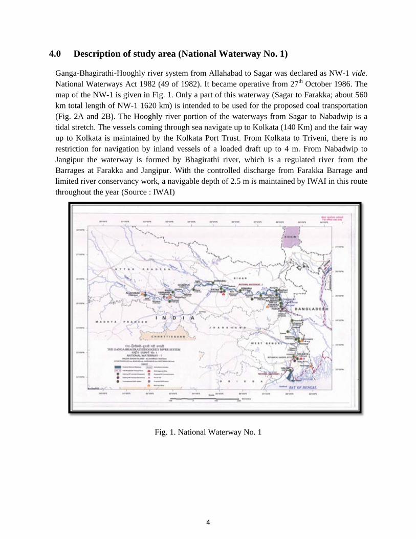
4.0 Description of study area (National Waterway No. 1) Ganga-Bhagirathi-Hooghly river system from Allahabad to Sagar was declared as NW-1 vide.
National Waterways Act 1982 (49 of 1982). It became operative from 27th October 1986. The map of the NW-1 is given in Fig. 1. Only a part of this waterway (Sagar to Farakka; about 560 km total length of NW-1 1620 km) is intended to be used for the proposed coal transportation (Fig. 2A and 2B). The Hooghly river portion of the waterways from Sagar to Nabadwip is a tidal stretch. The vessels coming through sea navigate up to Kolkata (140 Km) and the fair way up to Kolkata is maintained by the Kolkata Port Trust. From Kolkata to Triveni, there is no restriction for navigation by inland vessels of a loaded draft up to 4 m. From Nabadwip to Jangipur the waterway is formed by Bhagirathi river, which is a regulated river from the Barrages at Farakka and Jangipur. With the controlled discharge from Farakka Barrage and limited river conservancy work, a navigable depth of 2.5 m is maintained by IWAI in this route throughout the year (Source : IWAI)
Fig. 1. National Waterway No. 1

5
Fig. 2A. Sagar Island to Farakka stretch of National Waterway No.1 with location of Sand heads and Kanika Sands
6
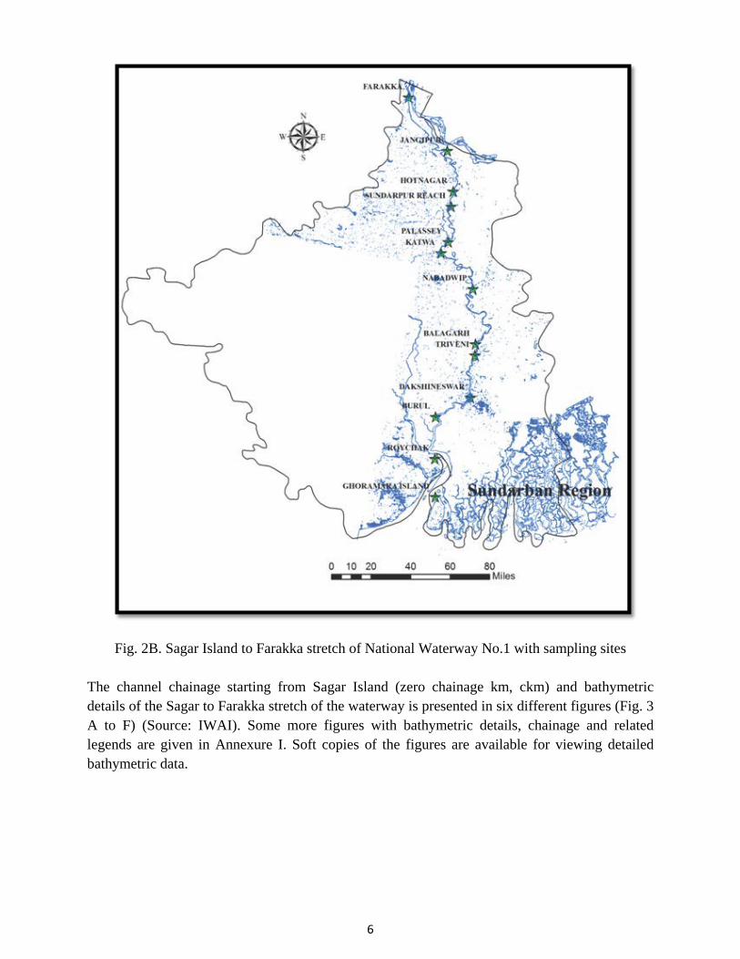
Fig. 2B. Sagar Island to Farakka stretch of National Waterway No.1 with sampling sites
The channel chainage starting from Sagar Island (zero chainage km, ckm) and bathymetric details of the Sagar to Farakka stretch of the waterway is presented in six different figures (Fig. 3 A to F) (Source: IWAI). Some more figures with bathymetric details, chainage and related legends are given in Annexure I. Soft copies of the figures are available for viewing detailed bathymetric data.

7
Fig. 3A. Sagar to Nayachar stretch of National Waterway No. 1 (The notations along the water way namely 63, 84, etc.represent water depth as 6.3 m, 8.4 m and so on)

8
Fig. 3B. Nayachar to Ravindra Setu (Kolkata) stretch of National Waterway No. 1 (The notations along the water way namely 63, 84, etc.represent water depth as 6.3 m, 8.4 m and so on)

9
Fig. 3C. Ravindra Setu (Kolkata) to Mongal Island (Balagarh) stretch of National Waterway No. 1 (The notations along the water way namely 63, 84, etc.represent water depth as 6.3 m, 8.4 m and so on)

10
Fig. 3D. Sabuj Island (Balagarh) to Phulbagan (Katwa) stretch of National Waterway No. 1 (The notations along the water way namely 63, 84, etc. represent water depth as 6.3 m, 8.4 m and so on)
11
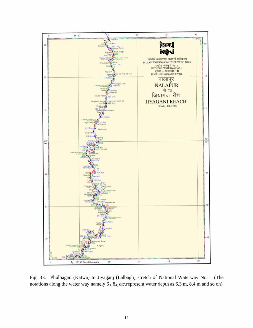
Fig. 3E. Phulbagan (Katwa) to Jiyaganj (Lalbagh) stretch of National Waterway No. 1 (The notations along the water way namely 63, 84, etc.represent water depth as 6.3 m, 8.4 m and so on)

12
Fig. 3F. Biswanathpur (Lalbagh) to Farakka stretch of National Waterway No. 1 (The notations along the water way namely 63, 84, etc.represent water depth as 6.3 m, 8.4 m and so on)

13
5.0 Coal loading/unloading and transportation system in place The related information has been provided by Jindal ITF regarding the coal handling at loading and unloading points and transportation as well as the facilities in place for waste management. A transshipper has been positioned at high seas at Sand heads under the jurisdiction of Kolkata Port during fair weather conditions and at Kanika Sands under jurisdiction of Paradip Port during rough weather conditions of monsoon months. Coal is unloaded into barges using transshipper and transported through NW-1 to NTPC, Farakka where a service platform equipped with cranes and conveyor system has been constructed for unloading and delivery to the NTPC stack yard. The Jindal ITF has elaborated that the Company has Standard Operating Procedures (SOPs) with regard to action required to be taken to prevent spillage and pollution during the operation and also in emergencies. The facilities, infrastructure and equipment involved in the process of transportation and handling used are given below.
5.1 Transshipment points
Transshipper is used (holding capacity of 66,000 ton and loading/unloading capacity 12,500 ton/day) to unload coal from Ocean Going Vessels (OGV) and loading onto the barges at Sand heads (Sagar) or Kanika Sands. Mechanical grabs available on the transshipper are used for trans-loading of coal into barges. These grabs are kept in perfect order so that they are locked face to face to avoid any spillage while discharging (Fig. 4). These mechanical grabs are so made that they cannot be lifted unless closed properly. Crane operators and signal men perform the task and ensure no draining of cargo while loading and no leakage from grab takes place outside the cargo holds. Additionally, cargo slings used are made of very strong canvas placed between the ships and the barges. Spillage, if any, is collected in the canvas. Cleaning gang cleans cargo spilled on the deck and puts it back in the cargo hold. Rubber sheets have been provided at the end of conveyor and boom so that even when cargo drops from a height, cargo will not fly into air. Immediately after loading the cargo in the barges, they are fully covered with tarpaulins before the barge sails out.
Fig. 4. Unloading of coal from ship to barge at Sand heads

14
5.2 The barges
The imported coal is trans-loaded into barges with carrying capacity of about 2,100 tons, but the actual quantity being carried depends on draft available. Presently a total of 23 barges are being engaged. The barges have dimension of 72 x 14 x 4.25 m (Fig. 5). They move at a speed of about 5 to 6 knots in loaded condition and about 9 to 11 knots while returning from Farakka in ballast. Thus, the average speed is 7-8 knots per hour and it takes about 5 to 6 days to complete its cycle of transportation. All barges are IRS (Indian Register of Shipping) class. The cargo is covered and secured properly with tarpaulin to ensure no spillage, as mentioned. Regarding the management of the pollutants generated in the barges, the disposable pollutants as listed below are disposed through work order issued to third party for collection of sludge at Coal Handling Plant (CHP) at Farakka. During full operation, it is proposed that about 40 barges will run throughout the year.
Fig. 5. Coal laden barge on its way
5.2.1 Used oil management
The waste oil used during servicing of the vessel machinery is stored in the bilge holding tanks. As per orders no pollutants or oils contained within bilges are to be pumped overboard into the river /sea. When the tank is nearing filling, the same is communicated to the control room for its disposal at Farakka.
5.2.2 Sewage management
Sewage Treatment Plant (STP), on the barges, is operational and running continuously. As per instructions, no direct discharge to the river / sea is undertaken. The disposable sewage is stored in sewage tank and discharged to shore support base at Nurpur. When the tank is nearing filling, the same is communicated to Operations Centre for arrangement of its disposal.
5.2.3 Garbage management
The galley /accommodation garbage is kept in disposable bags and stored in garbage bins. When the vessel reaches Nurpur, the garbage is disposed.

15
5.2.4 Bunkering of barges Jindal ITF Ltd. has a dedicated High Speed Diesel (HSD) Tanker unloading point along with a pump for transferring HSD from tanker to the barges (Fig. 6). Two flexible hose are used at two end points of a steel pipe fitted permanently for transfer. No leakages and spillage are ensured during transfer. Bunkering is done simultaneously at the time of unloading.
Fig. 6. Bunkering arrangements at Farakka
5.3 Coal Handling Plant (CHP) at Farakka
Jindal ITF Ltd, Farakka, as explained, has two service platforms (Fig. 7) at Farakka waterfront for unloading coal from barges and has invested in state of art CHP consisting of two grab un-loaders and dedicated coal conveying system (Fig. 8; 2.2 km with rated capacity of 800 ton per hour). The system is designed for environment friendly zero spillage/ zero dust emission while discharging/ unloading coal from barges.
Fig. 7. Coal unloading point at Farakka
16
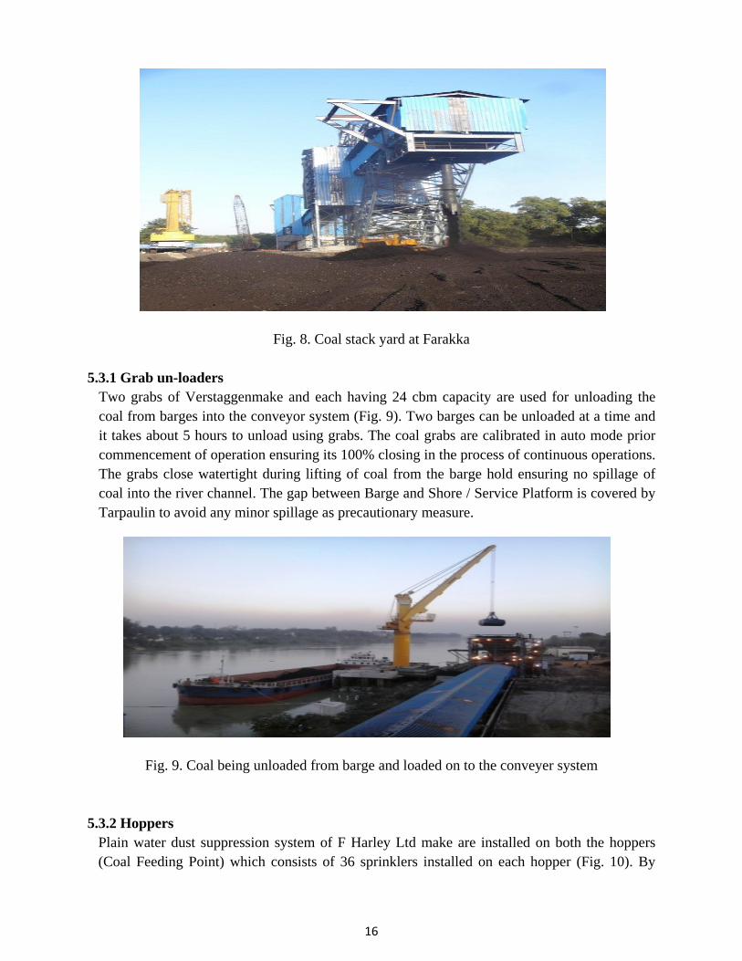
Fig. 8. Coal stack yard at Farakka
5.3.1 Grab un-loaders Two grabs of Verstaggenmake and each having 24 cbm capacity are used for unloading the
coal from barges into the conveyor system (Fig. 9). Two barges can be unloaded at a time and it takes about 5 hours to unload using grabs. The coal grabs are calibrated in auto mode prior commencement of operation ensuring its 100% closing in the process of continuous operations. The grabs close watertight during lifting of coal from the barge hold ensuring no spillage of coal into the river channel. The gap between Barge and Shore / Service Platform is covered by Tarpaulin to avoid any minor spillage as precautionary measure.
Fig. 9. Coal being unloaded from barge and loaded on to the conveyer system
5.3.2 Hoppers Plain water dust suppression system of F Harley Ltd make are installed on both the hoppers
(Coal Feeding Point) which consists of 36 sprinklers installed on each hopper (Fig. 10). By

17
sprinkling water through nozzles from all four sides of hopper dust generation is prevented and the same settles into the hopper.
Fig. 10. Sprinkling water to suppress coal dust 5.3.3 Junction houses Dry Fog Dust Suppression system, F Harley Ltd. make is installed on all junction Houses.
Plain water is mixed with compressed air, in the ratio 60:30, to create a dry fog. Droplets of water are atomized with the help of pressurized air and sprayed on the escaping dust to settle them on the conveyor belts.
5.3.4 Coal slurry management system Concrete Drains are laid alongside the Conveyors to collect the slurry which transfers the
slurry to coal settlement tank. After settlement and recirculation of the slurry, the clear water is collected and further pumped ahead to NTPC Sewage Treatment Plant. This ensures no slurry being discharged into the river (Fig. 11).
Fig. 11. Collection system for coal slurry

18
5.3.5 Pollution aspects of the environment in Coal Handling Plant As per the guidelines received from the State Pollution Control Board, Jindal ITF Ltd will have to generate data at half yearly interval on ambient air quality and liquid discharge systems. The analysis report is submitted to the Pollution Control Board office for inspection.
5.4 Disaster Management Emergency situation may arise during transshipment, operation of the barges or in the Coal Handling Plant. These may be dangerous to human life, environment, flora & fauna. To prevent such situation the following steps are to be taken:
• Minimize risk occurrence (Prevention) • Rapid control (Emergency Response) • Effectively Rehabilitate Damaged Areas (Restoration)
The major hazards may include Fire, Flood and Oil Spill. The safety measures covered under the Manual IWAI ; SOPs (Environment, health and safety manual of Jindal ITF Ltd.; Technical SOP of Jindal ITF Limited) are to be strictly followed. The following conditions may arise in river operations
• Grounding of vessel • Collision of vessel with cargo vessel • Collision of vessel with country boat carrying cargo • Collision of vessel with ferry boat carrying passengers • Collision of vessel with small country crafts • Collision of vessel against river/ canal bank • Collision of vessel with shore structures like bridges, HT line, • Fire Hazard • Spillage of oil in the river
Mitigation Measures
Facilities available and activities of IWAI: IWAI Nodal officers are available for day to day operation for the stretches : Sagar-Kolkata; Kolkata-Triveni; Triveni-Berhampore and Berhampore-Farakka. On receiving intimation of any distress the nodal officer of concerned area would alert the Distress Management Unit of IWAI, nearest Police Station, local administration, and would visit the site and coordinate deployment of multi-purpose tugs equipped with fire fighting facilities, first aid kit and life saving equipment immediately. The nodal officer of IWAI will alert the police.
A coordinating cum monitoring office at IWAI Regional Office, Kolkata, is being maintained for round the clock monitoring of the Inland Waterways.
Rescue Stations have been sited at Kolkata, Berhampore/Swaroopganj and Farakka which are equipped with high speed launches/boat fitted with additional life saving gears, fire fighting and first aid facilities.

19
Multipurpose tug (MPT) has been positioned at rescue stations for rescue/salvage operation including control/removal/arresting oil spillage.
Kolkata Port Trust /State Govt. agencies are sensitized for assistance in salvage/rescue operation.
Sensitization of users of the waterway including fishermen, passenger ferry operation, and country craft and general public of the area are also done.
Facilities available and activities of Jindal ITF Ltd. :
Quick reporting system is available through handheld VHF Radio sets or walkie talkies available in all barges.
Control Room is being manned 24x7 & for barge movement tracking and monitoring at Kolkata and at Farakka.
Emergency contact details to include district administration officials, police, hospitals, fire stations are available in all barges and Control Room.
Designated Person Ashore (DPA) has been nominated to monitor and act in case of emergency.
Barge crew has been trained to handle emergency situations such as fire, grounding, and collision with ferry boat.
In case of an accident the same to be informed by barge Master to nodal officer of the concerned stretch and Control Room either on mobile or through internet.
Incident Reporting/Near Miss Reporting & root cause analysis for the same is being carried out and circulated for awareness of the entire fleet.
Vessel movement is being done on designated Electronic Navigational Charts (ENC) track developed by IWAI containing information on general, topography, hydrography and navigational aids for safe navigation
River notices issued by IWAI fortnightly are being incorporated to ensure updation of track.
Dredging is being done by IWAI for maintaining ‘Least Available Depth’ (LAD) of 2.5 meters.
All vessels are being equipped with standard firefighting equipment.
SOP of the barge: In case of disaster incident while moving through water ways the SOPs complied with are: Technical SOP of Jindal ITF Ltd: Laid down safety procedures for compliance keeping in mind the safety of men and equipment. It also defines the various procedures to ensure environmental protection and maintaining highest standards of discipline in connection to pollution management. It also quantifies the various emergency procedures and drills to void such situation.
SOP of IWAI : An SOP has been formulated by IWAI to ensure safe navigation through channel and for assistance during disaster management.
20
SOP of Coal Handling Plant at Farakka: In case of disaster at plant site, it deals with Employee Health & Safety (EHS) SOP.
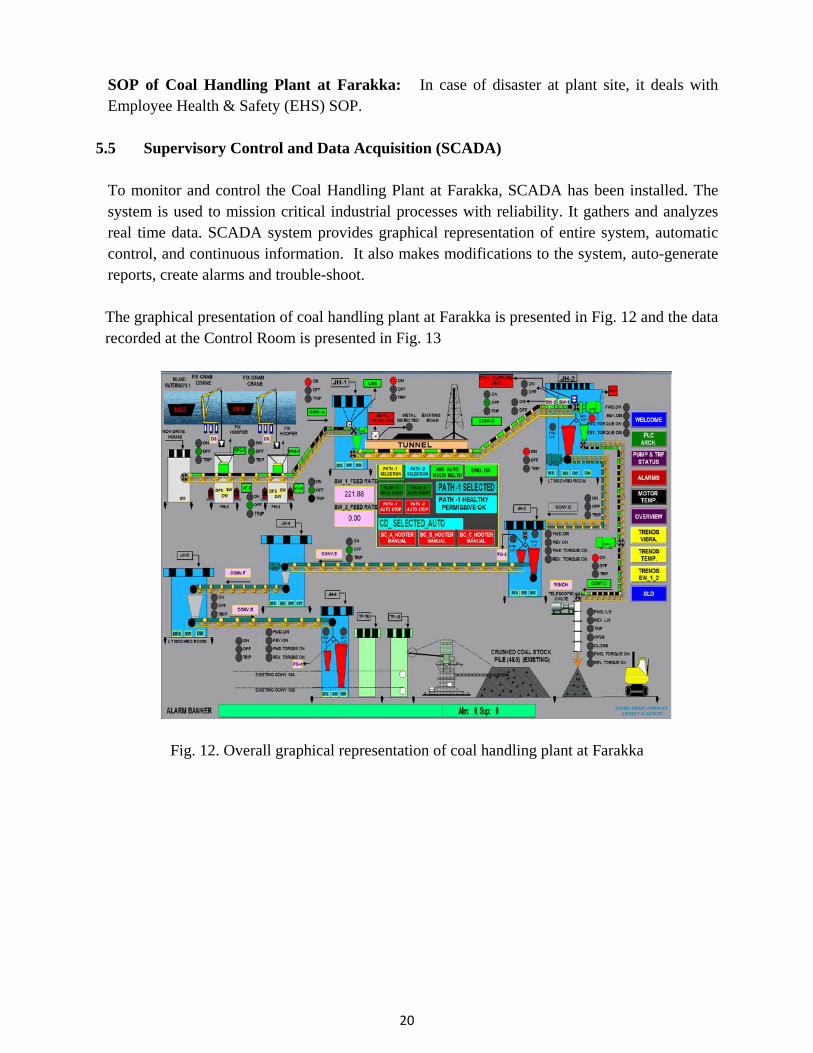
5.5 Supervisory Control and Data Acquisition (SCADA)
To monitor and control the Coal Handling Plant at Farakka, SCADA has been installed. The system is used to mission critical industrial processes with reliability. It gathers and analyzes real time data. SCADA system provides graphical representation of entire system, automatic control, and continuous information. It also makes modifications to the system, auto-generate reports, create alarms and trouble-shoot. The graphical presentation of coal handling plant at Farakka is presented in Fig. 12 and the data recorded at the Control Room is presented in Fig. 13
Fig. 12. Overall graphical representation of coal handling plant at Farakka

21
Fig. 13. Continuous equipment or process parameter Information at Control room

22

23
6.0 Details of studies conducted by CIFRI
A field study was undertaken by CIFRI, Barrackpore, in the Sagar Island to Farakka stretch of river Bhagirathi-Hooghly during March to August 2014 to generate information for achieving the major 3 objectives of the project. For convenience and comparison, the studied river stretch was divided into 3 zones namely –
Zone I: Lower zone from Sagar Island to Dakshineswar (154 km stretch) with characteristics of high shipping activities
Zone II: Middle zone from Dakshineswar to Nabadwip (124 km stretch) with characteristics of moderate shipping activities and
Zone III: Upper zone from Nabadwip to Farakka (282 km stretch) with characteristics of least shipping activities
Since ecology of an ecosystem is very important in regulating the abundance and distribution of biotic community, the basic parameters influencing ecology were studied. Present status of water and sediment quality parameters were recorded in 5 sampling sites from lower stretch, 3 sites from middle and 6 sites from upper stretch. The present values were compared with the previous observations to understand the changes occurred in the river stretch.
A significant amount of organic matter enters into any flowing system and is partly utilized in the production process, termed as allochthonus input. At the same time, the planktons capable of photosynthesis serve as the primary producers. The zooplankton community surviving on the primary producers are transferring the energy to the secondary and tertiary consumers. A portion of this energy is harvested as fish flesh. Thus, keeping in view the importance of planktons, the distribution of phyto- and zoo-planktons was studied in detail with zone wise abundance.
Since the benthic community are very good indicators about the local conditions, they were recorded in all the sampling sites. Their abundance and diversity were recorded.
Aquatic and embankment vegetation has a great role on aquatic ecology. These were studied along with the associated fauna.
Fish species availability was studied in detail during present survey and also listed from previous studies made at CIFRI. Zone wise distribution of fishes has been recorded along with diversity indices. Species distribution as per IUCN list has been discussed. Probable impact of coal laden barges on fish, its breeding and migration has been discussed based upon existing literature.
Pollution is a common problem encountered in inland aquatic ecosystems and present status of metal pollution has been discussed in the study.
It is anticipated that the fisher folk will be affected maximum due to frequent movement of barges which may hamper fishing operations. Thus, sample survey was conducted covering all the three stretches of study. The results have been discussed in detail with the perceptions of

24
fishers related to probable impact of barge movement on their economic condition and future scenario. A detailed delineation has been made on the fishing gears presently in use in the surveyed stretch. The study will help in analysis of post operational impact evaluation. An effort has been made to get an estimate about the number of fishers actually involved in fishing operations in the studied stretch.
It is anticipated that the physical movement of barges will cause some alterations in natural movement of water, will cause sediment suspension and bank erosion. Thus, a detailed study was conducted with model experimentation and analyzing historical satellite images and correlated the data to understand natural erosion. Critical speeds of the barges have been worked out to provide advice for minimizing erosion and movement associated problems.
6.1 Physico-chemical features of water
Rivers like Ganga have been the cradle of ancient civilizations of India where river banks were mostly preferred for human settlement. Even today population density is much higher around the river and that too is increasing day by day. Unfortunately, this population growth leads to increased anthropogenic pressure on the river, resulting in severe degradation of the ecosystem. River became the ultimate sink of anything and everything coming through surface runoff and in the bargain it is losing its utility functions at a faster pace. Water quality parameters have their direct influence on aquatic organism present therein. Biodiversity of rivers are modified as per the changes in habitat which is related to water quality parameters. So, continuous monitoring of water quality is necessary to formulate suitable management norms to prevent any unwanted modification of aquatic biodiversity. The parameters intimately associated with the aquatic organism were analyzed and presented below with a note of their importance. Graphical presentations are given for clear understanding of spatio-temporal changes of the parameters. The generated data are presented in the Table 2A, 2B and 3A, 3B at the end of the section.
6.1.1 Water temperature Among physical properties, water temperature is of prime importance as it controls all metabolic activities including growth of all aquatic organisms. It also controls some other related events like solubility of oxygen in water, decomposition of bottom organic matter for nutrient release, etc. Though thermal stratification was observed in lentic deeper water body, high flow and tidal action coupled with wind induced churning prevent any such thermal stratification in Hooghly-Bhagirathi river system. A temperature range of 15-35°C is suitable for fishes though lower temperature hinders their growth as observed during winter season. Water temperature directly depends on climate, sunlight, depth, water transparency etc. A depth of 1-2 mts considered optimal for biological productivity of a water body. If the depth is very less, water gets overheated and thus has an adverse effect on the survival of the fish. Carps grow better in the temperature range of 20-30 °C, whereas moderate growth is observed at a temperature range of 13-20 °C. For reproduction, carps need a temperature greater than 18°C. Higher water temperature was recorded during our monsoon survey as compared to pre-monsoon survey (Fig. 14). Increasing trend of water temperature was noticed from Farakka to Triveni during both the surveys, whereas tidal stretch showed decreasing trend from Dakshineswar to Ghoramara.

25
05
101520
Wat
er d
epth
(m) Pre-monsoon Monsoon
Rain decreased water temperature at Uluberia and Burul as compared to nearby stations during premonsoon.
Fig 14. Spatio-temporal changes of water temperature 6.1.2 Water depth River depth is cited as having an important role in migration of Tenualosa ilisha from sea
through the estuarine corridor to river Hooghly for breeding which prefers about 5.2 m depth for their migration (Bhaumik et al., 2011). Up to 3-4 m variation in river depth is quite common especially in gradient and marine zone sampling centers in Hooghly estuary due to semi-diurnal tidal rhythm. During early part of twentieth century, Hora (1943) reported severe scarcity of freshwater discharge through the river Hooghly with evidence of ‘a foot depth’ of water in parts of Hooghly during low tide. Higher freshwater discharge through feeder canal in post-Farakka period increased the water depth of Hooghly estuary significantly. The same locations as indicated by Hora (1943), are now retaining about 6-7 m water depth throughout the year. Not much variation between pre-monsoon and monsoon survey in water depth was observed during our survey which may be due to regulated release of water through feeder canal feeding the whole Hooghly-Bhagirathi river system (Fig. 15). Observed water depth variation was due to change in season, some variations in sampling site and in the estuarine stretch due to variations in tide. The bathymetric details of the river stretch are already given in Fig. 3A to 3F. In some of the sites of the navigation channel the depth has been noticed to be very low of about 3 m.
Fig.15. Spatio-temporal changes of water depth
2526272829303132333435
Tem
pera
ture
OC
Pre-monsoon Monsoon
26
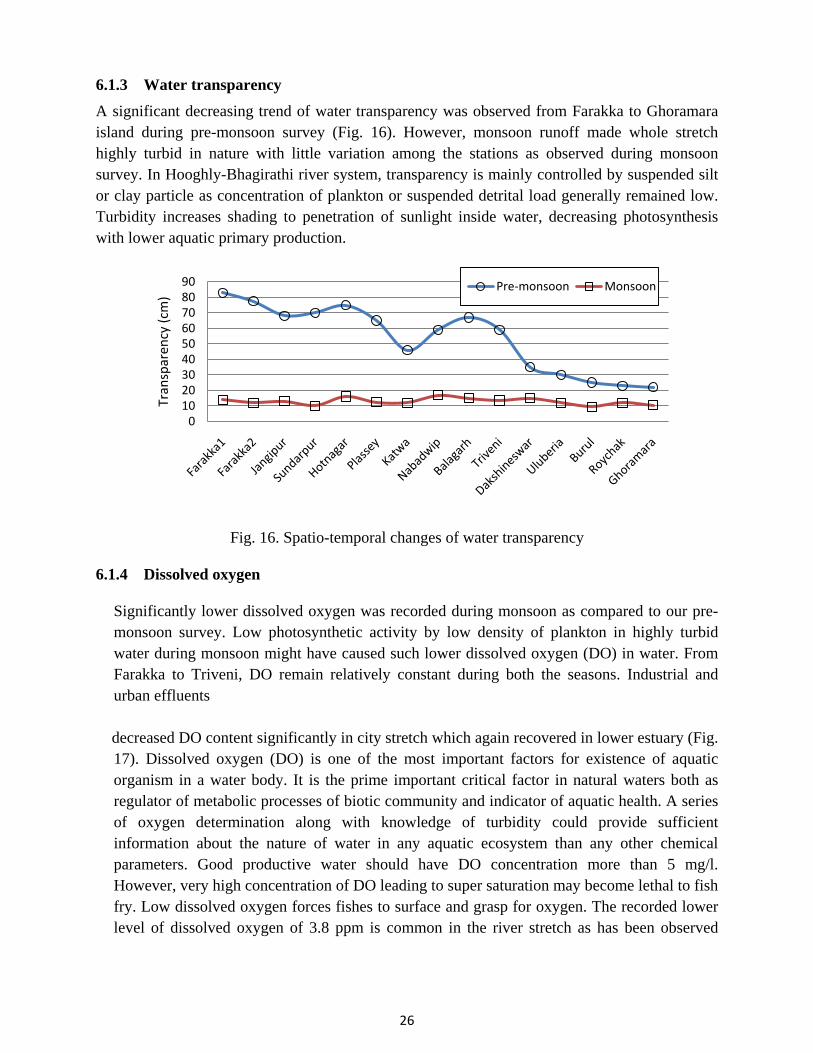
6.1.3 Water transparency A significant decreasing trend of water transparency was observed from Farakka to Ghoramara island during pre-monsoon survey (Fig. 16). However, monsoon runoff made whole stretch highly turbid in nature with little variation among the stations as observed during monsoon survey. In Hooghly-Bhagirathi river system, transparency is mainly controlled by suspended silt or clay particle as concentration of plankton or suspended detrital load generally remained low. Turbidity increases shading to penetration of sunlight inside water, decreasing photosynthesis with lower aquatic primary production.
Fig. 16. Spatio-temporal changes of water transparency 6.1.4 Dissolved oxygen Significantly lower dissolved oxygen was recorded during monsoon as compared to our pre-
monsoon survey. Low photosynthetic activity by low density of plankton in highly turbid water during monsoon might have caused such lower dissolved oxygen (DO) in water. From Farakka to Triveni, DO remain relatively constant during both the seasons. Industrial and urban effluents
decreased DO content significantly in city stretch which again recovered in lower estuary (Fig.
17). Dissolved oxygen (DO) is one of the most important factors for existence of aquatic organism in a water body. It is the prime important critical factor in natural waters both as regulator of metabolic processes of biotic community and indicator of aquatic health. A series of oxygen determination along with knowledge of turbidity could provide sufficient information about the nature of water in any aquatic ecosystem than any other chemical parameters. Good productive water should have DO concentration more than 5 mg/l. However, very high concentration of DO leading to super saturation may become lethal to fish fry. Low dissolved oxygen forces fishes to surface and grasp for oxygen. The recorded lower level of dissolved oxygen of 3.8 ppm is common in the river stretch as has been observed
0102030405060708090
Tran
spar
ency
(cm
)
Pre-monsoon Monsoon

27
earlier (reports on Survey of river Ganga 2012-13 of CIFRI and data of CPCB, MoEF, Government of India).
Fig. 17. Spatio-temporal changes of dissolved oxygen 6.1.5 Water pH Lowering of water pH from Triveni onwards was observed during our both the surveys (Fig.
18). This was due to the entry of effluents into the river. Decomposition of sewage organic matter releases CO2 and humic acid to make water acidic. However, water remained alkaline at all centers, a prime requisite for survival and growth of fishes as water pH in the range of 7.0-8.0 is known to be ideal for fish growth. Low pH caused acid stress, respiratory problem and mucus secretion on gills of fishes. On the other hand, higher pH damages gill, eye lens, cornea and disturbs acid-base balance of blood of fishes. Fishes was observed to tolerate a pH range of 4.8 to 10.8. Reproduction and growth of fishes was observed to diminish at pH less than 6.4 or more than 9.5. High pH is normally associated with a higher photosynthetic activity in water as observed through increased pH during our pre-monsoon survey. Plankton / macrophyte bloom caused higher pH during day hours due to absorption of CO2 (even by breaking HCO3
- in absence of CO2) for higher photosynthetic activity resulting in release of OH- in the system and thereby increasing pH.
Fig. 18. Spatio-temporal changes of water pH
3456789
10Di
ssol
ved
oxyg
en (m
g/l o
r pp
m)
Pre-monsoon Monsoon
77.27.47.67.8
88.28.48.6
pH
Pre-monsoon

28
6.1.6 Free CO2 Higher photosynthetic activity in relatively transparent water during pre-monsoon made
Farakka to Dakshineswar stretch without any free CO2 (Fig. 19). City effluent has its influence behind the presence of free CO2 at Uluberia. During monsoon, low plankton density in highly turbid water resulted in low photosynthetic activity not utilizing all free CO2 content in water and hence it was recorded at all the stations. Dissolved inorganic carbon, carbon-di-oxide and bicarbonate are the sources of carbon for photosynthesis of plankton as well as submerged aquatic plants and hence they can directly control the growth of them. Free CO2 is directly utilized by aquatic plants for photosynthetic activity. As surface water involved higher rate of photosynthesis, concentration of free CO2 is generally observed less in surface as compared to bottom. Due to very high consumption of free CO2 in surface water of a eutrophic water body, it may be absent during most period of the day except early morning and late afternoon hours. Though the use of HCO3
- is less efficient than free CO2 use causing lower photosynthetic rate, absence of free CO2 in eutrophic water body indicated possible HCO3
- use for photosynthesis.
Fig. 19. Spatio-temporal changes of free CO2
6.1.7 Total alkalinity Alkalinity or acid combining capacity of natural fresh water is generally caused by carbonates
and bicarbonates of calcium and magnesium, Ca being the dominating constituent. Dissolved CO2 in water forms an equilibrium with them which is of prime importance in determining productivity of aquatic ecosystem. Natural water containing 40 mg/l (or ppm) or more total alkalinity (TA) are more productive. The greater productivity of waters of higher alkalinity is not due to alkalinity directly, but in turn from phosphorus and other nutrients that increase with TA. Thus, TA could be a good index of productivity when phosphorus is not a limiting factor. During pre-monsoon, total alkalinity was much higher (112-115 mg/l) as compared to monsoon (56-90 mg/l) (Fig. 20). But, spatial variation is less during pre-monsoon as compared to monsoon.
-0.50
0.51
1.52
2.53
3.5
Free
CO
2(m
g/l o
r ppm
) Pre-monsoon Monsoon

29
Fig. 20. Spatio-temporal changes of total alkalinity 6.1.8 Total hardness Total hardness (TH) refers to the concentration of divalent metal ions in water, expressed as
mg/l of equivalent CaCO3 which is usually related to total alkalinity as the anions of alkalinity and the cations of hardness are normally derived from the solution of carbonate minerals. TH is significant in connection with pollution like sewage effluent. Ecosystems having moderately hard (61-120 mg/l) to hard (120-180 mg/l) water are more productive as it reflects the trends of Ca and Mg concentration in water. If TA falls low 15 mg/l, the water develops low buffering capacity. Again, very high TA (>200 mg/l) coupled with low TH (<20 mg/l) results in the rise in pH during afternoon beyond 11.0 and may cause death to fish. During pre-monsoon, total hardness was significantly higher in freshwater stretch as compared to total hardness in monsoon (Fig. 21). Total hardness starts increasing from Uluberia onwards during both the seasons due to mixing of saline water during high tide. Roychak and Ghoramara island observed higher total hardness due to ingress of sea water.
Fig.21. Spatio-temporal changes of total hardness
405060708090
100110120130
Alka
linity
(mg/
l or p
pm)
Pre-monsoon Monsoon
406080
100120140160180
Hard
ness
(mg/
l or p
pm) Pre-monsoon Monsoon
40
540
1040
1540
2040
2540
Hard
ness
(mg/
l or p
pm)

30
6.1.9 Specific conductivity Specific conductivity showed similar trend of hardness as saline water controls both the
parameters. Specific conductivity is an index of the amount of water soluble salts present in water. It also dictates the state of mineralization in an aquatic ecosystem. The soluble salts may be harmful to the aquatic life, not necessarily due to toxicity but due to changes in osmotic pressure. It increases with mineralization, and so higher sp. conductivity was observed in older water than newly entered water in a water body. Hence, higher sp. conductivity was recorded during pre-monsoon as compared to monsoon (Fig. 22). Saline water intrusion made sp. conductivity higher in Roychak and Ghoramara island.
Fig.22. Spatio-temporal changes of specific conductivity
6.1.10 Salinity Salinity is the key parameter controlling distribution of fish and other aquatic organisms in
any estuary. Monsoon freshwater inflow made Roychak a freshwater zone (0.27 ppt) as compared to 1.6 ppt recorded during pre-monsoon survey (Fig. 23). Salinity at Ghoramara island used to be strongly influenced by tidal action. Higher value of salinity at Ghoramara island during monsoon may be attributed to sampling during high tide. Based on salinity, Hooghly estuary was demarcated into three zones both in pre- and post-Farakka barrage period by several researchers. During pre-Farakka barrage period, due to lack of freshwater discharge, freshwater zone was small, stretching about 110 km from Nabadwip to Barrackpore. Even up to 1.16 ppt salinity was recorded at Barrackpore by David (1954) during pre-Farakka barrage period. However, increased freshwater inflow by water diversion through Farakka barrage changed the entire salinity scenario of the Hooghly estuary. Similar range of salinity that was observed by David (1954) at Barrackpore – Nawabganj region may now be found beyond Uluberia region, about 60 km downstream. Lal (1990) mentioned about 45 km shifting of freshwater zone limit from Konnagar (22°41ʹ58ʺN, 88°21ʹ41ʺE) to Uluberia (22°28ʹ02ʺN, 88°07ʹ10ʺE) in his study of the impact of Farakka barrage freshwater discharge. Change in zonation based on salinity in pre- and post-Farakka barrage period are reviewed in
4090
140190240290340390440490
Spec
ific
cond
uctiv
ity (µ
S/cm
) Pre-monsoon Monsoon
40
5040
10040
15040
20040
25040
Spec
ific
cond
uctiv
ity (µ
S/cm
)

31
details recently by Manna et al. (2013). Salinity around Ghoramara island was not much high due to higher freshwater discharge from upstream though it is near the estuarine mouth.
Fig. 23. Spatio-temporal changes of salinity
6.1.11 Biochemical oxygen demand Biochemical Oxygen Demand (BOD) is a measure of the amount of dissolved oxygen
required for biochemical degradation of organic material and oxidation of inorganic material like S2- or Fe2+. A method known as the standard 5-day BOD determination normally is used to estimate BOD5. Initial DO of the water is measured and final DO is measured after incubation of BOD bottle with water in the dark for 5 days at 20°C. The difference between initial and final DO gives an estimate of BOD. BOD is an important parameter for understanding anthropogenic pollution like untreated sewage discharge into rivers as BOD represents the amount of DO that will be used up in decomposing readily oxidizable organic matter. In case of high pollution, BOD test is performed with dilution by distilled water when dilution factor is used for calculation. BOD generally increases, as water remains stagnant for longer duration. Though Hooghly-Bhagirathi river system receives lot of pollution from cities and towns along the river, BOD level was not much higher mainly due to dilution by large volume of water diverted from Farakka barrage as well as ingress of sea water during high tide (Fig. 24). Effluent discharge point generally observed very high BOD, which reduces after some distance due to dilution by mixing with river water. Pre-monsoon survey observed higher BOD than that in monsoon at most of the stations during our survey. At Triveni, during monsoon, a significantly higher BOD was recorded which reduced slowly in downstream stations.
00.010.020.030.040.050.060.070.08
Salin
ity (p
pt)
Pre-monsoon Monsoon
02468
101214
Salin
ity (p
pt)

32
Fig.24. Spatio-temporal changes of biochemical oxygen demand
In December 1984, the MoEF, Government of India, prepared an action plan for immediate reduction of pollution load of the Ganga to bathing standard (DO not <5 ppm; BOD not >3 ppm, coliforms not >10,000 per 100 ml). The Government of India approved this as Ganga Action Plan (GAP) in April 1985. According to Ganga Action Plan, the data developed in the Hooghly river indicated that the stretch below Palta, the average BOD load reaches more than 3.0 during the premonsoon months when the head water discharge remains relatively low. The effect is well understood from the data of Central Pollution Control Board (Table 1). In the present study, although the recorded BOD was up to 3.1ppm, the dissolved oxygen was recorded to the value as low as 3.8 ppm during monsoon sampling at Uluberia-Burul stretch.
Table 1. Average BOD load of river Hooghly in different years
Year Stretch of Ganga 2011 2010 2003 1993 1986 Palta 2.1 1.6 2.4 2.7 1.0 Dakshineswar 4.0 4.2 3.8 - - Uluberia 2.8 3.2 5.5 1.9 1.1 Diamond Harbour 2.3 4.2 1.3 - -
(Source: CPCB, 2009, 2013)
6.1.12 Chemical oxygen demand Lower chemical oxygen demand was observed at most of the stations during monsoon survey
as compared to pre-monsoon (Fig. 25). This is due to dilution by monsoon rain which decreased the amount of oxidizable organic matter per unit volume. Though untreated municipal wastewater discharge is quite high in city stretch, dilution by large volume of water kept COD within the limit in lower stretch of river Ganga.
00.5
11.5
22.5
33.5
4
BOD
(mg/
l or p
pm)
Pre-monsoon Monsoon

33
Fig. 25. Spatio-temporal changes of chemical oxygen demand 6.1.13 Soluble reactive phosphate phosphorus (SRP) Significantly lower PO4-P during our pre-monsoon survey may be due to its rapid utilization
by higher plankton density in relatively transparent water (Fig. 26). High turbidity during monsoon prevents plankton to do intense photosynthetic activity where PO4-P is utilized. Phosphorus is often considered to be the most critical single element in the maintenance of aquatic productivity. Phosphorus fertility for aquatic productivity ranges from 0.05 to 0.20 mg/l. Phosphorous is the main factor behind eutrophication of a water body. In tropical waters due to high temperature, phosphate was rapidly assimilated (95% within 20 minute) by plankton and micro-organisms and hence available phosphate concentration is always very low. Mineralization of dead organic matter at sediment surface releases phosphorous, it will be absorbed by the sediment unless it is quickly absorbed by plankton, aquatic plants or bacteria. Phosphate is trapped as FePO4 or Al PO4 in acidic sediment and Ca3(PO4)2 in alkaline sediment.
Fig. 26. Spatio-temporal changes of PO4-P
6.1.14 Total Nitrogen Total inorganic or available nitrogen in water is contributed by NH4
+, NO2- and NO3
-. Dilution during monsoon caused lowering of total N as observed during our survey though
456789
1011
COD
(mg/
l or p
pm) Pre-monsoon Monsoon
0
0.02
0.04
0.06
0.08
0.1
0.12
Conc
n. o
f PO
4-P
(mg/
l or
ppm
)
Pre-monsoon

34
there are reports of higher nitrogen especially NO3-N in river water during monsoon through run-off. Nitrogen, a major constituent of protein occupies a predominant place in aquatic ecosystem. When bacteria decompose dead organic matter, part of the nitrogen in organic matter is converted to organic nitrogen in microbial biomass and the remainder is released to the water as ammonia. Nitrate produced in nitrification of ammonia can be absorbed by plants and bacteria. Under anaerobic condition, nitrate can be transformed to nitrite, ammonia or nitrogen gas by denitrification. Dissolved inorganic nitrogen in the range of 0.2 to 0.5 mg/l may be considered favourable for fish productivity. Ammonia, is also produced by fish and all other animals, including ourselves, as part of normal metabolism. Fish excrete metabolic ammonia directly into the surrounding water via special cells in the gills. Being toxic, most animals immediately convert it to a less harmful substance, usually urea, and excrete it through urine. Ammonia is also produced from decomposing fish food, fish waste and detritus. At low levels (<0.1 mg/l NH3), it acts as strong irritant, especially to the gills. Prolonged exposure to sub-lethal levels can lead to skin and gill hyperplasia (secondary gill lamellae swell and thicken, restricting the water flow over the gill filaments) causing respiratory stress. Fish response to sub lethal levels are similar to those to any other form of irritation, i.e. flashing and rubbing against solid objects. At higher levels (>0.1 mg/l NH3) even relatively short exposures can lead to skin, eye, and gills damage. Normal ammonia excretion from gills suppresses. Rise in blood-ammonia levels results in damage to internal organs. Fish response to toxic levels would be lethargy, loss of appetite, laying on pond bottom with clamped fins, or gasping at water surface if the gills are affected. The water ammonia contents during the sampling periods are presented in Fig. 27.
Fig. 27. Spatio-temporal changes of NH4-N
6.1.15 Silicate-Si Silicon, structural constituent of diatoms, remains as silicate form in natural waters. Normally
1-30 mg/l silicate-silicon or more remains present in Indian natural waters. At high temperature and pH, the solubility of silica increases greatly. In general, inverse relation exists
00.05
0.10.15
0.20.25
0.30.35
0.4
NH 4-
N (m
g/l o
r ppm
)
Pre-monsoon Monsoon

35
between salinity and silicate in estuaries indicating that silicate is mainly controlled by freshwater discharge. Decreasing trend of silicate from freshwater zone to marine zone was reported by Nandy et al. (1983). Sarma et al. (1993) observed highly significant inverse correlation of silicate and salinity in Godavari river estuary. We have come across similar decreasing trend of silicate from freshwater to saline zone during our study. During pre-monsoon, sharp declining trend was observed from Burul downwards, whereas sharp decline of silicate-silica was observed from Roychak to Ghoramara during monsoon (Fig. 28).
Fig. 28. Spatio-temporal changes of silicate-silica
Among the two sampling sites of Farakka, variations in water quality parameters were not
noticed.
0
2
4
6
8
10
12
Silic
ate
-Si (
mg/
l or p
pm)
Pre-monsoon Monsoon

36
Table 2A.Physico-chemical parameters of water (pre-monsoon)
Stations 1 2 3 4 5 6 Centers Farakka1 Farakka2 Jangipur Sundarpur Hotnagar Plassey Katwa Parameters 1. Date of sampling 26.03.14 26.03.14 27.03.14 27.03.14 28.03.14 28.03.14 29.03.14 2. Time 10.45AM 12.00PM 09.30AM 12.15 PM 07.45AM 11.00AM 08.00AM 3. Weather Clear Clear Clear Clear Clear Clear Clear 4. Air Temp. (°C) 31.0 35.0 33.0 35.0 29.0 36.0 30.5 5. Water Temp. (°C) 26.0 26.0 26.7 27.0 26.8 27.6 27.1 6. Avg. Depth (m) 7.31 7.31 3.23 17.98 15.24 7.62 9.33 7. Transparency(cm) 83 77.5 68 70 75 65 46 8. DO (ppm) 8.8 8.7 8.4 8.8 8.2 8.2 8.0 9. pH 8.34 8.34 8.29 8.41 8.33 8.37 8.33 10. Free CO2 (ppm) 0 0 0 0 0 0 0 11. Carbonate (ppm) 8 8 7 12 8 8 12 12. Bicarbonate (ppm) 106 106 107 103 106 107 101 13. Alkalinity (ppm) 114 114 114 115 114 115 113 14. Hardness (ppm) 138 138 136 138 138 139 138 15. Sp. conduct. (µS/cm) 344 344 343 347 346 346 344 16. BOD (ppm) 2.8 3 2.5 3.1 2.7 2.2 2.6 17. COD (ppm) 6.8 6.8 8.0 8.0 8.4 7.6 10.4 18. PO4-P (ppm) 0.0084 0.0084 0.0073 0.0081 0.0081 0.0081 0.0069 19. Total NH4-N (ppm) 0.2164 0.1272 0.205 0.3168 0.313 0.1244 0.0518 20. Silicate (ppm) 4.563 4.456 5.365 4.367 4.654 4.349 4.214 21. Salinity (ppt) 0.0519 0.0513 0.051 0.0401 0.0527 0.0513 0.052
Table 2B.Physico-chemical parameters of water (pre-monsoon)
Stations 7 8 9 10 11 12 13 14 Centers Nabadwip Balagarh Triveni Dakshineswar Uluberia Burul Roychak Ghoramara
Island Parameters
1. Date 30.03.14 31.03.14 01.04.14 03.04.14 05.04.14 06.04.14 07.04. 14 08.04.14 2. Time 08.30AM 07.45AM 07.00AM 08.45AM 07.30AM 07.00AM 07.30AM 07.30AM 3. Weather Clear Clear Clear Clear Clear Clear Clear Clear 4. Air Temp. (°C) 30.0 30.0 29.0 31.0 29.0 27.0 29.3 29.3 5. Water Temp. (°C) 27.4 27.8 27.9 28.8 27.0 26.3 29.0 29.0 6. Avg. Depth (m) 4.57 10.24 5.64 5.49 9.14 12.80 9.63 13.72 7. Transparency(cm) 59 67 59 35 30 25 23 22 8. DO (ppm) 8.2 8.35 8.6 7.0 5.0 4.6 6.0 6.6 9. pH 8.41 8.43 8.46 8.16 8.00 7.78 7.87 7.91 10. Free CO2 (ppm) 0.0 0.0 0.0 0.0 3.0 3.0 2.4 0.0 11. Carbonate (ppm) 10 10 10 8 0 0 0 6 12. Bicarbonate (ppm) 105 104 102 104 115 115 119 110 13. Alkalinity (ppm) 115 114 112 112 115 115 119 116 14. Hardness (ppm) 138 137 138 136 154 154 480 1610 15. Sp. Conduct.
(µS/cm) 344 342 346 350 410 461 3210 13550
16. BOD (ppm) 3.0 2.2 2.6 2.6 2.8 2.7 2.5 3.0 17. COD (ppm) 6.4 9.2 7.6 7.2 7.8 8.4 - - 18. PO4-P (ppm) 0.0058 0.0081 0.007 0.0246 0.031 0.0353 0.0379 0.0453 19. Total NH4-N (ppm) 0.1222 0.085 0.1536 0.117 0.08 0.0624 0.0762 0.0568 20. Silicate (ppm) 4.657 4.336 4.342 4.957 4.474 5.137 3.164 2.645 21. Salinity (ppt) 0.05325 0.05773 0.05443 0.0548 0.06812 0.05805 1.6 7.9

37
Table 3A. Physico-chemical parameters of water (monsoon) 1 2 3 4 5 6 Sl. No. Centre Farrakka1 Farrakka2 Jangipur Sundarpur Hotnagar Plassey Katwa 1. Date 10.07.14 10.07.14 09.07.14 11.07.14 12.07.14 16.07.14 17.07.14 2. Time 9:00 AM 11:00 AM 9:15 AM 9:45 AM 9:30 AM 9:30 AM 8:00 AM 3. Weather Clear Clear Clear Clear Clear Clear Cloudy 4. Air temp. (ᵒC) 34.3 33.6 34.2 36.3 34.8 33.8 30.9 5. Water temp. (ᵒC) 30.9 31.1 31.1 31.9 32.1 32.1 31.9 6. Avg. Depth (m) 8.23 9.853 7.013 7.113 7.47 3.35 3.98 7. Transparency (cm) 14 12 13 10 16 12.5 12 8. DO (ppm) 6.0 5.44 4.2 5.96 5.68 6.2 6.2 9. pH 8.1 7.95 7.34 8.14 7.95 7.88 8.08 10. Free CO2 (ppm) 1.6 2.4 2.2 1.8 0.8 1.2 0.6 11. Carbonate (ppm) - - - - - - - 12. Bicarbonate (ppm) 68 64 56 62 62 68 68 13. Total alkalinity (ppm) 68 64 56 62 62 68 68 14. Total hardness (ppm) 72 66 56 72 68 78 80 15. Sp. Conduct. (µS/cm) 174 167 133 177 176 184 196 16. BOD (ppm) 0.24 0.12 0.2 0.2 0.2 0.68 1.2 17. COD (ppm) 5.2 7.2 6.8 6.8 6.8 4.8 6.4 18. PO4-P (ppm) 0.0405 0.0438 0.0728 0.0634 0.0716 0.0564 0.026 19. Total NH4-N 0.0075 0.0939 0.0010 0.0028 0.0018 0.0006 0.0011 20. Silicate (ppm) 6.684 7.158 9.789 7.947 6.947 5.789 5.316 21. Salinity (ppt) 0.0419 0.0408 0.039 0.0401 0.0394 0.0408 0.039 Table 3B. Physico-chemical parameters of water (monsoon) Stations 7 8 9 10 11 12 13 14 Sl. No. Centers Nabadwip Balagarh Triveni Dakshine
swar Uluberia Burul Roychak Ghoramara
Island Tide HT HT LT HT LT HT LT Parameters 1. Date 17.07.14 19.07.14 20.07.14 14.07.14 28.07.14 30.07.14 29.07.14 31.07.14 2. Time 10:30 AM 8:00 AM 8:30 AM 8:00 AM 1:30 PM 8:10 AM 11:00 AM 1:00 PM 3. Weather Cloudy Clear Cloudy Cloudy Rainy Clear Cloudy Cloudy 4. Air Temp. (°C) 32.5 32.0 31.2 33.1 30.3 32.3 31.1 33.3 5. Water Temp. (°C) 31.1 32.0 33.8 32.5 32.5 31.7 31.4 31.9 6. Avg. Depth (m) 3.92 8.53 7.16 7.47 8.23 4.37 4.27 5.49 7. Transparency(cm) 17.0 15.0 13.5 15.0 12.0 9.5 12.0 10.5 8. DO (ppm) 6.1 5.8 5.9 5.1 4.0 3.8 5.2 6.2 9. pH 7.95 8.02 8.02 7.92 7.95 7.88 7.99 7.95 10. Free CO2 (ppm) 0.8 1.4 1.0 0.6 1.2 0.8 1.0 1.6 11. Carbonate (ppm) - - - - - - - - 12. Bicarbonate (ppm) 68 68 72 68 82 80 80 90 13. Alkalinity (ppm) 68 68 72 68 82 80 80 90 14. Hardness (ppm) 74 76 80 72 92 98 124 2200 15. Sp. Conduct. (µS/cm) 191 193 199 193 225 226 673 19720 16. BOD (ppm) 0.88 0.24 2.88 1.92 1.16 0.96 0.64 0.92 17. COD (ppm) 6.4 6.4 7.6 4.8 8.0 9.6 15.6 18. PO4-P (ppm) 0.0519 0.0558 0.0365 0.0583 0.0994 0.0877 0.0753 0.0809 19. Total NH4-N(ppm) 0.0014 0.0015 0.0047 0.0028 0.0014 0.0015 0.0026 0.0027 20. Silicate (ppm) 5.947 6.526 6.421 8.737 7.474 7.737 8.158 3.895 21. Salinity (ppt) 0.0401 0.0491 0.043 0.039 0.049 0.0509 0.2683 11.943

38
6.2 Physico-chemical features of sediment
Along with water quality parameters the sediment quality parameters were analyzed for the sampling sites. The data are presented in the end of the section in Table 4A, 4B and 5A, 5B. Like water, sediment parameters were assessed in two sites of Farakka.
6.2.1 Sediment texture Based on size, sediment particles have been grouped into three categories viz. clay (<0.002
mm dia.), silt (0.002 - 0.02 mm dia.) and sand (>0.02 mm dia.). Too much clay dominated soils are not desirable for fisheries as it adsorbs nutrients making them unavailable to water phase for use by primary producers. Sandy soils, on the other hand, does not store nutrient at all, which is also not good for productivity. Loamy soil with a balanced combination of sand, silt and clay is most desirable for any water body. During pre-monsoon, river bottom was mostly sandy in nature at all the sampling stations. During monsoon, surface run-off increased silt percentage at some stations especially in lower stretch except at Burul. The high sand content at Burul during all the seasons is utilized for sand mining during low tide. Clay content was generally low except at few stations with slightly higher values. In city stretch sampling stations like Balagarh, Triveni, Dakshineswar observed slightly higher values.
6.2.2 Sediment pH Sediment pH of a water body is one of the most important critical factors as it controls all
chemical reactions like mineralization, availability of phosphorus, etc. Growth and survival of benthic communities are also governed by soil pH. Acidic soils are undesirable for fish productivity as it does not support microbial activity. Neutral to slightly alkaline soil is most desirable for better productivity.
During monsoon survey, slightly lower pH was observed at most of the stations of the studied
stretch (Fig. 29). However, during both the seasons sediment at all the stations was alkaline in nature.
Fig. 29. Spatio-temporal variation of sediment pH
77.27.47.67.8
88.28.48.68.8
pH
Pre-monsoon Monsoon
39
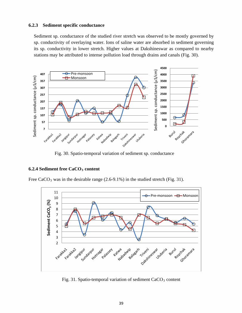
6.2.3 Sediment specific conductance Sediment sp. conductance of the studied river stretch was observed to be mostly governed by
sp. conductivity of overlaying water. Ions of saline water are absorbed in sediment governing its sp. conductivity in lower stretch. Higher values at Dakshineswar as compared to nearby stations may be attributed to intense pollution load through drains and canals (Fig. 30).
Fig. 30. Spatio-temporal variation of sediment sp. conductance 6.2.4 Sediment free CaCO3 content Free CaCO3 was in the desirable range (2.6-9.1%) in the studied stretch (Fig. 31).
Fig. 31. Spatio-temporal variation of sediment CaCO3 content
7
57
107
157
207
257
307
357
407
Sedi
men
t sp.
con
duct
ance
(µS/
cm) Pre-monsoon
Monsoon
0
500
1000
1500
2000
2500
3000
3500
4000
4500
Sedi
men
t sp.
con
duct
ance
(µS/
cm)
23456789
1011
Sedi
men
t CaC
O3
(%)
Pre-monsoon Monsoon

40
0
5
10
15
20
Sedi
men
t ava
ilabl
e N
(m
g/10
0g)
Pre-monsoon Monsoon
6.2.5 Sediment organic carbon
Variation in sediment organic carbon is mostly governed by amount of organic matter coming through surface run-off with little contribution from plankton. It acts as a direct source of energy to microbes present in soils that take part in mineralization. Soils with less than 0.5% organic carbon are considered as less productive. 0.5-1.5% and >1.5% organic carbon are considered as medium and high productive category. In the excess accumulation of organic matter, anaerobic condition is developed at bottom which may produce toxic gases detrimental to fish. The observed organic matter content was in the normal range (Fig. 32).
Fig. 32. Spatio-temporal variation of sediment organic carbon
6.2.6 Sediment nitrogen
Sediment nitrogen is one of the major controlling factors to control aquatic productivity. It remains mostly in organic form and mineralized by soil microbes to be liberated as different ions like NH4
+, NO3-, NO2
-, etc. for utilization by plankton in water phase. For any productive soil, available nitrogen must be above 250 mg/kg. However, in the studied stretch sediment available N was low due to sandy nature and low organic C of the bottom (Fig. 33). Increased silt load during monsoon may have contributed in increased available N in most of the stations.
Fig. 33. Spatio-temporal variation of sediment available N
00.10.20.30.40.50.60.7
Sedi
men
t org
anic
car
bon
(%)
Pre-monsoonMonsoon

41
6.2.7 Sediment total N
Sediment total N was low during both the seasons at all the sampling centers due to sandy river bed with low organic C (Fig. 34).
Fig. 34. Spatio-temporal variation of sediment total N
6.2.8 Sediment available phosphorous
Phosphorus is essential for nitrogen assimilation in cellular matter besides different metabolic functions like protein synthesis, respiration, cell division etc. Phosphorus is mostly present in soils as insoluble ferric and aluminium phosphate in acid soils and as calcium phosphate in alkaline soils. A soil must have above 3 mg/100 g available phosphorus for good productivity. Higher percentage of sand and low organic C in river bottom might have played the role behind lower available P (up to the maximum of 2 mg/100 g) in bottom sediment in all the sampling stations (Fig. 35).
Fig. 35. Spatio-temporal variation of sediment available P
00.010.020.030.040.050.060.070.080.09
0.1
Sedi
men
t tot
al N
((%
) Pre-monsoon Monsoon
0
0.5
1
1.5
2
2.5
Sedi
men
t ava
ilabl
e P
(mg/
100g
) Pre-monsoon Monsoon

42
6.2.9 Sediment C/N ratio
Less variations in sediment C/N ratio among the stations was observed during pre-monsoon as compared to monsoon (Fig. 36). Since the monsoon sampling was at the beginning of the season more seasonal variation was not noticed.
Fig. 36. Spatio-temporal variation of sediment C/N ratio
0
5
10
15
20
25
Sedi
men
t C/N
ratio
Pre-monsoon Monsoon
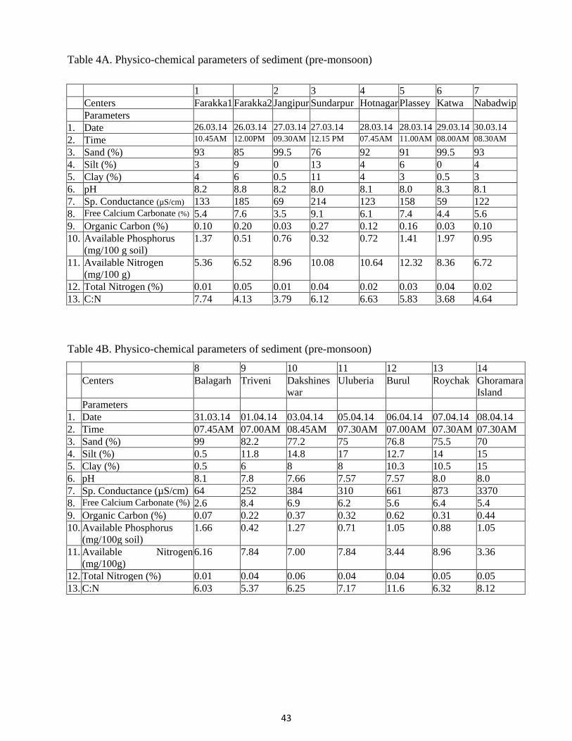
43
Table 4A. Physico-chemical parameters of sediment (pre-monsoon) 1 2 3 4 5 6 7 Centers Farakka1 Farakka2 Jangipur Sundarpur Hotnagar Plassey Katwa Nabadwip Parameters 1. Date 26.03.14 26.03.14 27.03.14 27.03.14 28.03.14 28.03.14 29.03.14 30.03.14 2. Time 10.45AM 12.00PM 09.30AM 12.15 PM 07.45AM 11.00AM 08.00AM 08.30AM
3. Sand (%) 93 85 99.5 76 92 91 99.5 93 4. Silt (%) 3 9 0 13 4 6 0 4 5. Clay (%) 4 6 0.5 11 4 3 0.5 3 6. pH 8.2 8.8 8.2 8.0 8.1 8.0 8.3 8.1 7. Sp. Conductance (µS/cm) 133 185 69 214 123 158 59 122 8. Free Calcium Carbonate (%) 5.4 7.6 3.5 9.1 6.1 7.4 4.4 5.6 9. Organic Carbon (%) 0.10 0.20 0.03 0.27 0.12 0.16 0.03 0.10 10. Available Phosphorus
(mg/100 g soil) 1.37 0.51 0.76 0.32 0.72 1.41 1.97 0.95
11. Available Nitrogen (mg/100 g)
5.36 6.52 8.96 10.08 10.64 12.32 8.36 6.72
12. Total Nitrogen (%) 0.01 0.05 0.01 0.04 0.02 0.03 0.04 0.02 13. C:N 7.74 4.13 3.79 6.12 6.63 5.83 3.68 4.64 Table 4B. Physico-chemical parameters of sediment (pre-monsoon)
8 9 10 11 12 13 14 Centers Balagarh Triveni Dakshines
war Uluberia Burul Roychak Ghoramara
Island Parameters 1. Date 31.03.14 01.04.14 03.04.14 05.04.14 06.04.14 07.04.14 08.04.14 2. Time 07.45AM 07.00AM 08.45AM 07.30AM 07.00AM 07.30AM 07.30AM 3. Sand (%) 99 82.2 77.2 75 76.8 75.5 70 4. Silt (%) 0.5 11.8 14.8 17 12.7 14 15 5. Clay (%) 0.5 6 8 8 10.3 10.5 15 6. pH 8.1 7.8 7.66 7.57 7.57 8.0 8.0 7. Sp. Conductance (µS/cm) 64 252 384 310 661 873 3370 8. Free Calcium Carbonate (%) 2.6 8.4 6.9 6.2 5.6 6.4 5.4 9. Organic Carbon (%) 0.07 0.22 0.37 0.32 0.62 0.31 0.44 10.
Available Phosphorus (mg/100g soil)
1.66 0.42 1.27 0.71 1.05 0.88 1.05
11.
Available Nitrogen (mg/100g)
6.16 7.84 7.00 7.84 3.44 8.96 3.36
12. Total Nitrogen (%) 0.01 0.04 0.06 0.04 0.04 0.05 0.05 13. C:N 6.03 5.37 6.25 7.17 11.6 6.32 8.12

44
Table 5A. Physico-chemical parameters of sediment (monsoon)
1 2 3 4 5 6 7 Centers Farakka1 Farakka2 Jangipur Sundarpur Hotnagar Plassey Katwa Nabadwip Parameters 1. Date 10.07.14 10.07.14 09.07.14 11.07.14 12.07.14 16.07.14 17.07.14 18.07.14 2. Time 9:15 AM 11:15 AM 9:15 AM 9:45 AM 9:30 AM 9:30 AM 8:00 AM 10:30 AM 3. Sand (%) 93 54 93 78 53 70 81 79 4. Silt (%) 0.5 37 1 13 31 24 9 14 5. Clay (%) 6.5 9 6 9 16 6 10 7 6. pH 7.5 7.7 7.3 7.8 7.7 7.78 7.78 7.78 7. Sp. Conductance
(µS/cm) 112 199 94 114 134 121 124 130
8. Free CaCO3 (%) 5 8 5.5 6.5 6.75 7 6.5 4.5 9. Organic Carbon (%) 0.33 0.66 0.03 0.39 0.27 0.09 0.36 0.27 10.
Available Phosphorus (mg/100 g)
0.556 0.351 0.451 1.0689 1.032 1.057 0.437 0.529
11.
Available Nitrogen (mg/100 g)
5.04 9.52 8.96 9.52 19.04 14 2.8 7.84
12. Total Nitrogen (%) 0.02 0.04 0.01 0.04 0.02 0.03 0.04 0.05 13. C:N 14.56 16.26 2.90 10.61 11.42 3.38 8.04 5.08
Table 5B. Physico-chemical parameters of sediment (monsoon)
8 9 10 11 12 13 14 Centers Balagarh Triveni Dakshine
swar Uluberia Burul Roychak Ghoramara
Island Parameters 1. Date 19.07.14 20.07.14 14.07.14 28.07.14 30.07.14 29.07.14 31.07.14 2. Time 8:00 AM 8:30 AM 8:00 AM 1:30 PM 8:15 AM 11:00 AM 1:00 AM 3. Sand (%) 44 39 40 50 95 40 76 4. Silt (%) 40.5 45 46 42 3 52.5 11 5. Clay (%) 15.5 16 14 8 2 7.5 13 6. pH 7.71 7.75 7.3 7.47 7.78 7.74 7.82 7. Sp. Conductance (µS/cm) 179 164 332 238 177 323 3910 8. Free Calcium Carbonate
(%) 7.0 6.5 5.5 6.25 5.5 5.25 4.25
9. Organic Carbon (%) 0.36 0.30 0.33 0.06 0.09 0.345 0.27 10.
Available Phosphorus (mg/100 g)
0.372 0.443 0.728 0.508 0.565 0.466 0.511
11. Available Nitrogen (mg/100g)
16.24 15.12 13.12 13.44 3.36 8.96 2.24
12. Total Nitrogen (%) 0.02 0.05 0.09 0.03 0.03 0.02 0.03 13. C:N 21.43 6.49 3.80 1.95 2.78 14.49 7.71

45
6.3 Plankton Community
Plankton is the most sensitive floating community which is being the first target of water pollution, thus any undesirable change in aquatic ecosystem affects diversity as well as biomass of this community (Summarwar, 2012). The knowledge on the abundance, composition and seasonal succession of the same is a prerequisite for the successful management of an aquatic ecosystem. Phytoplankton are the primary producers for the entire aquatic body and comprise the major portion in the ecological pyramids. The community of phytoplankton especially the different species of diatoms are also used as indicator of water pollution. Zooplanktonic organisms are also known as bio-indicators of water quality and degree of pollution because they are strongly influenced by environmental alterations and respond quickly to changes in quality (Dorak, 2013). In the eutrophic water the zooplankton composition changes; replace the dominance from larger species (e.g. calanoid copepods) to smaller species (e.g. especially rotifers) (Marneffe et al., 1996). Zooplanktons are an important link in the transformation of energy from producers to consumers (Sharma et al. 2010). Hence, studies on plankton are important as because water flow and changes in the river hydromorphology, exerts an important control over lotic communities (Deksne et al., 2011). In the consumer food chain of aquatic ecosystems, zooplankton play an important role in the transfer of energy from the primary producer to fish. They play an important role in the natural food chain which constitute important food item of omnivorous and carnivorous fishes. Thus, to a large extent production of fish is dependent on the plankton community.
6.3.1 Phytoplankton
For quantitative analysis, 1 litre of water surface samples were collected using tube water sampler and fixed with 10 ml lugol's iodine solution (Baykal et al., 2011) in a polypropylene narrow mouth sample bottle (Tarson, India). Quantum of abundance was measured using haemocytometer (Neubauer - improved, marienfeld, Germany). Photographic data were recorded using a photo capture unit (Moticam 2300) digital microscopy. Algae were identified using different source (Prescott, 1899; Ramanathan, 1964; Philipose, 1967; Hustedt, 1976; Cox, 1996; Anand, 1998; Biggs and Kilroy, 2000). Phyla were arranged by algae base (Guiry and Guiry, 2013).
Phytoplankton have been represented by 31 genera belonging 4 phylum and 7 classes distributed among 15 orders and 23 families. Group wise distribution of important algal classes in the entire stretch showed that phytoplankton community are more diverse in Zone 1 i.e. Sagar Island to Dakshineswar with a dominant contribution by Bacillariophyceae (Table 6). The data indicates that the dominant algae in lower Ganga is Cyanophyceae and Chlorophyceae followed by Bacillariophyceae (IIT report, 2012). Diversity of Bacillariophyceae was observed in upper stretch i.e. Nabadwip to Farakka. Cyanophyceae was subdominant in the upper stretch. In total 14 taxa with a dominant group of Bacillariphyceae and Coscinodiscophyceae were reported from middle stretch from Dakshineswar to Nabadwip. Abundance of phytoplankton has been depicted based on presence and absence basis (Table 7). Quantified sample of phytoplankton collected from various stations has been

46
depicted. The observation showed that Zone 1 was more diverse with higher percentage of Coscinodiscophyceae (36%) and Fragilariophyceae (21%) followed by Chlorophyceae (18%), Cyanophyceae (7%), Trebouxiophyceae (7%), Conjugatophyceae (6 %) and Bacillariophyceae (5%) (Fig. 37). Present study showed that Fragilariophyceae were dominant with 32% among all the algae followed by Chlorophyceae (23%), Coscinodiscophyceae (18%), Trebouxiophyceae (17%) and Cyanophyceae (10%) in Zone II, Dakshineswar to Nabadwip (Fig. 38). The upper zone from Nabadwip to Farakka has been observed with high percentage of Coscinodiscophyceae (36%) and Fragilariophyceae (28%) followed by Cyanophyceae (14%) and Trebouxiophyceae (11%) (Fig. 39). A pictorial view of the phytoplankton profile in various zones has been shown in Fig. 40.
Distribution of algae in the entire study stretch has been represented as follows:
Zone I (Sagar Island to Dakshineswar): Surirella sp., Navicula sp., FragIlaria sp., Synedraulna, Cymbella sp., Nitzschia sp., Aulacoseiragranulata,Coscinodiscus sp., Cyclotella sp., Microcystis sp., Actinastrum sp., Pediastrum duplex.,Scenedesmus sp., Coelastrum sp., Spirogyra sp., Anabaena sp., Fragilariacrotonensis, Pleurosigma sp., Oscillatoria sp., Lyngbya sp., Phormidium sp., Merismopedia sp., Gloeocapsa sp., Gloeothece sp., Scenedesmusdimorphus, Scenedesmusquadricauda, Kirchneriella sp.
ZONE II (Dakshineswar to Nabadwip): Fragilaria sp., Synedra sp., Pinnularia sp., Nitzschia sp, Cymbellatumida, Aulacoseiragranulata, Coscinodiscus sp., Cyclotella sp., Microcystis sp., Spirulina sp., Oscillatoria sp., Actinastrum sp., Pediastrum sp., Ankistrodesmus sp., Staurastrum sp., Rhopalodia sp., Scenedesmusquadricauda, Merismopedia sp., Fragilariacrotonensis.
Zone III (Nabadwip to Farakka): Surirella sp., Navicula sp., Gomphonema sp.,Eunotia sp., FragIlaria sp., Synedra sp., Synedraulna, Pinnularia sp., Cymbella sp., Nitzschia sp., Aulacoseiragranulata, Coscinodiscus sp., Cyclotella sp., Microcystis sp., Spirulina sp., Oscillatoria sp., Actinastrum sp., Scenedesmusquadricauda., Hantzschia sp., Merissmopedia sp., Anabaena sp.
Table 6. Group wise distribution of important algal classes
Group No. of Taxa Species in different stretches Zone I Zone II Zone III
Bacillariophyceae 11 5 3 6 Frgilariophyceae 2 3 2 2 Coscinodiscophyceae 3 3 3 3 Cyanophyceae 9 6 2 5 Trebouxiophyceae 1 1 1 1 Chlorophyceae 5 6 2 1 Conjugatophyceae 3 1 1 0 Total 34 25 14 18

47
Table 7. Phytoplankton profile of river Bhagirathi-Hooghly
Zone I Zone II Zone III Phyllum: OCHROPHYTA Class: BACILLARIOPHYCEAE Order: Surirellales Family: Surirellaceae Surirella sp. - - + Order:Naviculales Family: Naviculaceae Navicula sp. + + - Family: Pleurosigmataceae Pleurosigma sp - - + Order: Cymbellales Family: Cymbellaceae Cymbella sp. + + - Cymbella tumida - + - Family: Gomphonemataceae Gomphonema sp. - - + Family: Pinnulariaceae Pinnularia sp. - + - Order: Bacillariales Family: Bacillariaceae Nitzschia sp. + + + Hantzschia sp. - - + Order Eunotiales Family Eunotiaceae Eunotia sp. - - + Order Rhopalodiales Family Rhopalodiaceae Rhopalodia sp. - + - Class: FRAGILARIOPHYCEAE Order: Fragilariales Family: Fragilariaceae Fragilaria sp. + + ++ Fragilaria crotonensis + + - synedra sp. + + + Synedra ulna - + + Synedra acus - - + Class: COSCINODISCOPHYCEAE Order: Coscinodiscales Family: Aulacoseiraceae Aulacoseira sp. + ++ ++ Family:Coscinodiscaceae Coscinodiscus sp. ++ - - Order: Thalassiosirales Family:Stephanodiscaceae Cyclotella sp. + + +

48
Zone I Zone II Zone III Phyllum: CYANOPHYTA Class: CYANOPHYCEAE Order: Chroococcales Family: Microcystaceae Microcystis sp. ++ ++ ++ Gloeocapsa sp. + - - Family Cyanobacteriaceae Gloeothece sp. + - - Family: Spirulinaceae Spirulina sp. - + - Order: Oscillatoriales Family: Oscillatoriaceae Oscillatoria sp. + + - Lyngbya sp. + + - Family Phormidiaceae Phormidium sp. + - - Phylum: CHLOROPHYTA Class: TREBOUXIOPHYCEAE Order: Chlorellales Family: Chlorellaceae Actinastrum sp. + ++ ++ Class CHLOROPHYCEAE Order Sphaeropleales Family: Hydrodictyaceae Pediastrum sp. ++ ++ + Pediastrum duplex + + - Family: Selenastraceae Ankistrodesmus sp. - + - Kirchneriella sp. + - - Family: Scenedesmaceae Scenedesmus sp. + - + Scenedesmus quadricauda + + + Scenedesmus dimorphus + + + Coelestrum sp. - - + Phylum: CHAROPHYTA Class: CONJUGATOPHYCEAE Order:Zygnematales Family: Zygnemataceae Spirogyra sp. + - - Order: Desmidiales Family: Closteriaceae Closterium sp. - - + Family: Desmidiaceae Staurastrum sp. - + -
‘+’ indicates presence; ‘-’ indicates absence; ‘++’ indicates dominance

49
Fig. 37. Phytoplankton density in Zone I, Sagar Island to Dakshineswar
Fig. 38. Phytoplankton density in Zone II, Dakshineswar to Nabadwip
Bacillariophyceae5%
Frgilariophyceae 21%
Coscinodiscophyceae
36%
Cyanophyceae 7%
Trebouxiophyceae7%
Chlorophyceae 18%
Conjugatophyceae6%
Frgilariophyceae 32%
Coscinodiscophyceae
18%Cyanophyceae
10%
Trebouxiophyceae17%
Chlorophyceae 23%

50
Fig. 39.Phytoplankton density in Zone III, Nabadwip to Farakka.
Fig. 40. Phytoplankton diversity in river Bhagirathi-Hooghly A) Actinastrum sp. B) Aulacoseira sp. C) Cyclotella sp. D) Pediastrumduplex E) Fragilaria sp.
F) Scenedesmus sp. G) Coscinodiscus sp. H) Surirella sp.
Bacillariophyceae11%
Frgilariophyceae 28%
Coscinodiscophyceae
36%
Cyanophyceae 14%
Trebouxiophyceae11%

51
6.3.2 Zooplankton
For quantitative analysis, 50 liters of water samples from below surface was collected following standard protocol (APHA, 2012) and preserved in 4% formaldehyde solution for further analysis. The density and abundance were estimated by using a compound microscope. Quantum of abundance was measured using sedge-wick rafter cell count method. Zooplankton community were identified at genus level. Photographic data were recorded using a photo capture unit (Moticam 2300) digital microscopy. Zooplankton was identified using various source (Battish, 1992; Edmondson, 1992; Witty, 2004).
Zooplankton community during present study period has been represented by 15 genus belonging 8 orders and 9 families. Abundance was depicted based on presence and absence basis (Table 8).
Table 8. Abundance and distribution of zooplankton
Stations Zone I Zone II Zone III
Phylum: Arthropoda Class: Maxillopoda Order: Calanoida Family: Diaptomidae Diaptomus sp. + - - Order: Cyclopoida Family: Cyclopidae Cyclops sp. ++ - - Class: Branchiopoda Order: Diplostraca Family: Bosminidae Bosmina sp. + + ++ Family: Moinidae Moina sp. + ++ ++ Family: Daphniidae Daphnia sp. - - + Family: Chydoridae Chydorus sp. - - + Alonella sp. - + - Family:Sididae Diphanosoma sp. - + + Phylum: Rotifera Class: Euotatoria Order: Ploima Family: Brachionidae Brachionus sp. + ++ + Keratella sp. + ++ ++ Family: Synchaetidae Polyarthra sp. - + - Order: Flosculariaceae Family: Trochosphaeridae Filinia sp. + + -
‘+’ indicates presence; ‘-’ indicates absence; ‘++’ indicates dominance

52
Distribution and level of dominance in various zones has been shown (Fig. 41, 42 and 43). From the quantitative study it can be concluded that copepods were dominant in all the three zones followed by cladocerans and rotifers with significant abundance in zone –I and zone –II. Diversity of zooplankton has been depicted in Fig. 44.
Copepods dominated in the zooplankton. Nauplii, Cyclops sp, Diaptomus sp are mostly comprising this group. Quantified study of zooplankton showed that copepods were dominant in zone-I during the present sampling, especially in Ghoramara, Dakshineswar and Burul. The present study also supports the observation made by Shetty et al.,(1956) in Dakshineswar. In zone II, the percentages of copepods found were - Triveni 44%, Balagarh 54.16%, Nabadwip 51.85%, Katwa 46.15%, respectively. Similarly in Zone-III, the percentage of the copepods were in Plassey 63.15%, Hotnagar 68.75%, Sundarpur 70.58%, Jangipur 38.88%, Farakka(1) 60%, Farakka(2) 44% respectively.
The different Cladocerans were Alonella sp, Diaphanosoma sp, Moina sp. In Zone I, the percentages of cladocerans were 23.07% in Roychak, 43.75% in Uluberia, where as in the other centres viz., Ghoramara Island, Burul and Dakshineswar, these were absent. In zone II, in Triveni 32.35%, Balagarh 20.83%, Nabadwip 29.62% and Katwa 15.38%, respectively. Similarly in Zone III- in Plassey 63.15%, Hotnagar 31.25%, Sundarpur 29.41%, Jangipur 22.22%, Farakka(2) 28%, respectively.
The Rotiferas were very common in fresh water. Brachionus sp., Keratella sp., Polyarthra sp., Filinia sp. were found during the monsoon season. Zone I was lack of Rotifera. In Zone II, these were found in Triveni 32.35%, Balagarh 25%, Nabadwip 18.51% and Katwa 18.51%, respectively. In zone III, the percentages of the Rotifers were in Jangipur 33.33%, Farakka(1) 35% and Farakka(2) 16%.
Fig. 41. Zooplankton profile in Zone 1 (Sagar Island to Dakshineswar)
Copepoda46%
Rotifera26%
Cladocera28%

53
Fig. 42. Zooplankton profile in Zone II (Dakshineswar to Nabadwip)
Fig. 43. Zooplankton profile in Zone III (Nabadwip to Farakka)
Fig. 44.Zooplankton diversity of river Bhagirathi-Hooghly A) Moina sp. B) Cyclops sp. C) Brachionus sp. D) Filinia sp. E) Nauplius F) Keratella sp. G) Bosmina sp.
Copepoda49%
Rotifera26%
Cladocera25%
Copepoda81%
Cladocera19%

54
Effect of coal laden / unladen barge movement on planktons
Review of literatures indicates that movement of barges cause alluvium, loose soil that is carried downstream and increase the suspended sediment loads. The unconsolidated soil is also accompanied with the presence of exposed tree roots, clumps of grass from collapsed river banks. Hence, eroded river bank acts as an external force on phytoplankton development. The situation enables low light permeability in underwater. Thus, light limitation derived from higher water turbidity would limit photosynthesis and prevent phytoplankton development (Reynolds, 2006; Baykal et al., 2011). Micro-zooplanktonic populations are important because they serve as the foundation for food chains supporting vertebrate populations (USEPA, 2011) and are sensitive biological indicators of biological impairment in aquatic ecosystems (Chadwick and Canton, 1983; USEPA, 2011).
The transportation of coal through barges under present project has been under operation for a short period of time (about 16 months). Thus, long term impacts could not be evaluated. However, it is recommended that regular monitoring should be undertaken to assess the impacts, if any.

55
6.4 Benthic Community
Aquatic environments are made up of complex interrelations between plant and animal species and their physical environment. Harm to the physical environment will often lead to harm for one or more species in a food chain which may lead to damage for other species. In open waters, fish and other large aquatic animal have ability to avoid unfavourable zone, reducing the likelihood impact. However, there are certain groups of aquatic sedentary animals having major role in food chain known as benthic invertebrates. Benthic invertebrates are animal such as worms, mussels, snails, crayfish, and immature forms of aquatic insects that lack backbones and live on the bottom of the river and generally have limited capability of movement. Usually, invertebrate densities are good indicators of water quality and health status of the rivers. Many diversity and biotic indices have been developed in temperate rivers to categorize the river types based on their degree of pollution and degradation.
For the present study, benthic diversity was studied by collecting the sample by standard methods. Samples were collected by Peterson grab (sampling area 780 cm2) from three random sites representing the entire river cross section at each sampling sites from Farakka to Sagar Island. The samples were grouped as microbenthos and macrobenthos based on their size. The zone wise diversity of the organisms collected during the month of July and August representing monsoon is depicted in Fig. 45. Zone I was dominated by Thiara(Tarebia) granifera with 19%, followed by Bellamya crassa with 16% and Bortia costula with 15% of total species diversity. Zone II was dominated by Thiara(Tarebia) granifera with 78% followed by polychaetae and Bortia costula with 5% of total species diversity. While Zone III was dominated by Neritina violacea with 34% followed by insect with 26% of the total species. Reports from other studies describes the presence of a total of 90 species under 66 genera of which 48 species of Polychaetes, 35 species of Oligochaetes and 7 species of Hirudinia were recorded. Maximum number of species were recorded from Zone III followed by Zone I and II. Further, the zone wise diversity of the organisms collected during the month of March-April representing pre-monsoon is depicted in Fig. 46(A,B,C). The diversity was more in Zone III (Farakka to Nabadwip, 11 genus with 18 species) than Zone II (Nabadwip to Dakshineswar, 10 genus with 13 species) and Zone I (Dakshineswar to Sagar, 7 genus with 8 species). The Zone-III was dominated by Thiara sp. followed by polychaeta and Corbicula bensoni. Zone-II was dominated by Thiara lineata followed by polychaeta and Novaculina gangetica. The zone-I was dominated by Thiara lineata followed by T. granifera and polychaeta. The percentage wise distribution is presented in Fig. 46. The diversity of the organisms depends on many factors. Anticipating the frequent movement of barges the effect caused thereto needs detailed study.
During sample collection, some deposition of coal particles was recorded in the river bed at Farakka sampling site 2 during July, 2014 which was a maximum up to 0.08% (w/w). To get a detailed picture on the level of spillage during unloading of coal from barges, a special sampling program was undertaken during December, 2014. During December sampling, sediment samples were collected at every 25 m downstream from the Jindal project site. It was observed that though some coal particles were present at the project site, its content has not increased from the first observations and no coal particles were detected in the sediment beyond 50 m. It has been

56
recorded that Jindal ITF is taking necessary precautions like use of tarpaulin sheets, operating grab unloaders only by related professionals, etc. The precautions were based upon the discussions made by CIFRI representatives with Jindal ITF officials. Probably some nominal spillage has happened during the initial stage of the project and now it is not happening. The benthic macro-invertebrates observed in the coal unloading site of Farakka 2 are given in Fig. 48. Although some amount of spillage was recorded in the site, no adverse effect was recorded due to it.
Fig. 45.Diversity and distribution of benthic organisms in Bhagirathi-Hooghly river during monsoon (July-August)
Bellamya crassa
Bellamya dissimilis
Bortia costula
Corbicula bensoni
Corbicula striatella
Gabbia orcula
Indoplanorbis exutus
Novaculina gangetica
Parreysia (R)lima
Polychaeta
Scapula deltae
Thiara(M)tuberculata
Thiara(Tarebia)granifera
Thiara(Tarebia)lineata
Zone -II
Bellamya bengalensis
Bellamya crassa
Bellamya dissimilis
Bortia costula
Parreysia (R)lima
Polychaeta
Stenothyra ornata
Thiara(Tarebia)granifera
Thiara(Tarebia)lineata
Zone IIIAmpoda
Bellamya bengalensis
Crab
Insecta
Neritina smithi
Neritina violacea
Novaculina gangetica
Pila globosa
Prawn seed
Telescopium telescopium
Thiara(Tarebia)lineata
Zone I
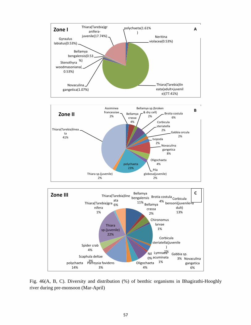
57
Fig. 46(A, B, C). Diversity and distribution (%) of benthic organisms in Bhagirathi-Hooghly river during pre-monsoon (Mar-April)
polychaeta(1.61%)
Neritina violacea(0.53%)
Thiara(Tarebia)lineata(adult+juvenil
e)(77.41%)
Novaculina gangetica(1.07%)
Stenothyra woodmasoniana(
0.53%)
Bellamya bengalensis(0.53
%)
Gyraulus labiatus(0.53%)
Thiara(Tarebia)granifera-
juvenile(17.74%)Zone I
Assiminea francessiae
2%Bellamya
crassa4%
Bellamya sp.(broken & dry cell)
2%Brotia costula
6%Corbicula steriatella
2%Gabbia orcula
2%Isopoda
2%Novaculina gangetica
8%
Oligochaeta4%
Pila globosa(juvenile)
2%
polychaeta23%
Thiara sp.(juvenile)2%
Thiara(Tarebia)lineata
41%
Zone II
Bellamya bengalensis
11% Bellamya crassa
2%
Brotia costula4%
Chironomus larvae
1%
Corbicula bensoni(juvenile+a
dult)13%
Corbicula steriatella(juvenile
)1%
Gabbia sp.3%
Lymnaea acuminata
1%
Nil0% Novaculina
gangetica6%
Oligochaeta4%
Parreysia favidens3%
polychaeta14%
Scaphula deltae3%
Spider crab4%
Thiara sp.(juvenile)
22%
Thiara(Tarebia)granifera
1%
Thiara(Tarebia)lineata6%
Zone III
B
A
C

58
Fig. 47. Tarpaulin sheet used to prevent coal particle scattering into the river
Fig. 48. Macrobenthos invertebrates collected from the river bed at Farakka
Benthic invertebrates are organisms that live on the bottom of a water body or in the sediment. These organisms play important role in nutrient cycling and form a vital component in aquatic food web. Like other organisms, the distribution and abundance of benthic invertebrates may be profoundly influenced by water and sediment quality parameters. Spatial and temporal differences in benthic species composition may also be influenced by a range of biological factors (e.g. primary productivity, competition and acclimatization). Natural seasonal and inter-annual changes in these variables can also modify recruitment success and mortalities of individual species, and consequently the community structure of the benthos. However, in recent years pollution such as industrial wastes, heavy metals and pesticides has created a havoc for these invertebrates. To record impact of barge movement on the benthic communities, long term studies are required and present observations will be the basis of evaluation.

59
6.5 Aquatic and shoreline vegetations High turbidity and high flow regime in river prevent infestation of aquatic macrophyte in entire studied stretch of the river. Also, at many places, river bank modification was made with boulders, concrete structure to avoid erosion. This also prevents growth of aquatic macrophyte. However, infestation by emergent variety of macrophyte is observed in the stretches of the river where shoreline remains relatively undisturbed. Kash grass (Saccharum spontaneum) quickly colonizes on exposed silt deposition after monsoon, and forms almost pure stands along the shoreline. Typha angustata, the cattail dominance was observed in shoreline near Lalbagh. Phragmites sp. dominance was observed near Nabadwip area. Other than emergent variety, semi-aquatic plants like Ipomea aquatica, Jussia repens etc were recorded in sampling centres of Bhagirathi river (Fig. 49-56).
Fig. 49. Typha angustata, cattail dominance in shoreline near Lalbagh
Fig. 50. Shoreline infestation with Saccharum spontaneum, (Kash in Bengali) in Balagarh
Fig. 51. Dense infestation of grass unable to prevent river bank erosion near Nabadwip
Fig. 52. Infestation of Phragmites sp. prevents shoreline erosion in Bhagirathi river

60
Fig. 53. Ipomea aquatica, (locally known as kolmi) survived high flow of Bhagirathi to proliferate along the shoreline
Fig. 54.Jussia repens, (locally known as Helencha) another macrophyte recorded from sampling stations of Bhagirathi river
Fig. 55. Aquatic macrophyte associated fauna - dragon-fly nymph, beetle, etc.
Fig. 56. Aquatic macrophyte associated mollusks
A list of grass and aquatic, semi terrestrial vegetation in Hooghly/ Bhagirathi adjacent area is presented in Table 9.
Table 9. List of grass and aquatic, semi terrestrial vegetation in Bhagirathi-Hooghly adjacent area
Sl. No. Vernacular name Scientific name 1. Ulu ghass Imperata cylindrica 2. Uri Dhan Oryza rufipogon 3. Kash Saccharum spontaneum 4. Kahon chal Setaria italic 5. Kush Desmostachya bipinnata 6. Khoskhos Vetiveria zizanioides 7. Dhadda Saccharum narenga 8. Nol Arundo donax 9. Khagra Phragmites karka

61
Sl. No. Vernacular name Scientific name
10. Mutha Cyperus rotundus 11. Gothubi Kyllinga monocephala 12. Chorkata Chrysopogon aciculatus 13. Durba ghass Cynodon dactylon 14. Kulekhara Hygrophila schulii 15. Hinche Enhydra fluctuans 16. Sachi Sakh Alternanthera philoxeroides 17. Kesute Eclipta prostrate 18. Kanchira Commelina diffusa 19. Choto pata Kanchira Commelina benghalensis 20. Thankuni Centella asiatica 21. Vuin Okra Phyla modiflora 22. Ravan Lata Stephania japonica 23. Kochu Colocasia esculenta 24. Ghechu Aponogeton natans 25. Jal dhone Ranunculus sceleratus 26. Ful jharu Thysanolaena maxima 27. Shyama Ghash Echinochloa crus-galii 28. Sabai Ghash Eulaliopsis binata 29. Pati Ghass Juncellus inundates 30. Jol Ghash Leersia hexandra 31. Topa pana Pistia stratiotes 32. Kochuripana Eichhornia crassipes 33. Jol Lojjaboti Neptunia oleracea 34. Dholkolmi Ipomoea fistulosa 35. Hogla Typha angustifolia 36. Kolmi Ipomoea aquatica 37. Susni Sakh Marsilea minuta 38. Bramhi Sakh Bacopa monnieri 39. Kalabati Canna indica
In the estuarine mouth areas the following mangrove and associated plants were recorded (Table 10). The zone is in the established shipping channel.
Table 10. Vegetations recorded in the estuarine mouth area
Sl. No. Vernacular name Scientific name 1. Sada Bain Avicennia alba 2. Piara Bain Avicennia marina 3. Kalo Bain Avicennia officinalis 4. Dhani Ghass Porteresia coarctata

62
6.6 Ichthyodiversity and associated studies
In India, the tributaries and distributaries of river Ganga basin supports rich biodiversity and offers livelihood and nutritional security to millions of riparian population. River Bhagirathi-Hooghly, declared as waterway No.1, is the part of mighty river Ganga which drains through the State of West Bengal into the Bay of Bengal. The river system harbours rich and diverse freshwater ichthyofauna along the stretch and many estuarine fishes in the lower reaches of the river. Freshwater fish are one of the most threatened taxonomic groups (Darwall and Vie, 2005) because of their high sensitivity to the quantitative and qualitative alteration of aquatic habits (Laffaille et al. 2005; Kang et al., 2009; Sarkar et al., 2008). As a consequence, they are often used as bioindicator for the assessment of water quality, river network connectivity or flow regime (Chovance et al., 2003). Today the fish diversity and associated habitat management is a great challenge (Dudgeon et al., 2006). Conservation measures to mitigate the impact of the pressures have largely been slow and inadequate and as a result many of the species are declining rapidly.
6.6.1 Fish Species Diversity
In order to explore the fish diveristy and abundance, the lower stretch of the river was surveyed during March-April, 2014 and July, 2014. Fish assemblages were studied through experimental fishing as well as analysing fishermens' catch. Species diversity, richness along with trophic and niche diversity were recorded. Altogether 225 fish species were recorded during the study from the entire stretch of Sagar Island toFarakka (Table 11).
Table 11: List of fish species recorded from the stretch of Ganga
S. No. Family Species name 1 Adrianichthydae Oryzias dancena 2
Ambassidae
Ambassis nalua 3 Chanda nama 4 Parambassis lala 5 Parambassis ranga 6 Anabantidae Anabas testudineus 7 Anguillidae Anguilla bengalensis bengalensis 8 Aplocheilidae Aplocheilus panchax 9
Ariidae
Arius arius 10 Arius gagora 11 Cephalocassis jatia 12 Hexanematichthys sagor 13 Osteogeneiosus militaris 14 Badidae Badis badis 15
Bagridae
Mystus bleekerii 16 Mystus cavasius 17 Mystus gulio 18 Mystus tengara 19 Mystus vittatus 20 Rita rita 21 Sperata aor 22 Sperata seenghala

63
23 Batrachiodidae Batraichthys grunniens 24 Belonidae Strongylura strongylura 25 Xenentodon cancila 26 Botiidae Botia dario 27 Botia lohachata 28 Bregmacerotidae Bregmaceros mcclellandi 29 Callionymidae Callionymus fluviatilis 30
Carangidae
Alepes kleinii 31 Gnathanodon speciosus 32 Megalaspis cordyla 33 Scomberoides commersonianus 34 Scomberoides lysan 35
Channidae
Channa marulius 36 Channa orientalis 37 Channa punctata 38 Channa striata 39 Cichlidae Oreochromis mossambicus 40 Oreochromis niloticus 41 Clariidae Clarias batrachus 42
Clupeidae
Anodontostoma chacunda 43 Corica soborna 44 Escualosa thoracata 45 Goniolosa manmina 46 Gudusia chapra 47 Sardinella gibbosa 48 Sardinella melanura 49 Tenualosa ilisha 50 Cobitidae Acanthocobotis botia 51 Lepidocephalus guntea 52
Cynoglossidae
Cynoglossus cynoglossus 53 Cynoglossus lingua 54 Cynoglossus puncticeps 55 Cynoglossus puncticeps 56 Paraplagusia bilineata 57
Cyprinidae
Amblypharyngodon mola 58 Aspidoparia jaya 59 Aspidoparia morar 60 Barbonymus altus 61 Bengala elanga 62 Catla catla 63 Chela cachius 64 Cirrhinus mrigala 65 Cirrhinus reba 66 Crossocheilus latius latius 67 Ctenopharyngodon idella 68 Danio devario 69 Danio rerio 70 Esomus danricus 71 Hypophthalmichthys nobilis 72 Labeo bata 73 Labeo calbasu

64
74 Labeo rohita 75 Laubuca laubuca 76 Osteobrama cotio 77 Puntius conchonius 78 Puntius gelius 79 Puntius phutunio 80 Puntius sarana sarana 81 Puntius sophore 82 Puntius terio 83 Puntius ticto 84 Rasbora daniconius 85 Rasbora rasbora 86 Salmophasia acinaces 87 Salmophasia phulo 88 Salmostoma bacaila 89 Securicula gora 90 Dasyatidae Dasyatis zugei 91 Himantura bleekeri 92
Eleotridae
Butis butis 93 Butis melanostigma 94 Eleotris fusca 95 Odonteleotris macrodon 96 Ophieleotris aporos 97
Engraulidae
Coilia dussumieri 98 Coilia neglecta 99 Coilia ramcarati 100 Coilia reynaldi 101 Setipinna breviflis 102 Setipinna phasa 103 Setipinna taty 104 Setipinna tenuifilis 105 Stolephorus baganensis 106 Stolephorus commersonii 107 Stolephorus indicus 108 Thryssa purava 109 Thryssa stenosoma 110 Erethistidae Erethistes pussilus 111 Gerreidae Gerres setifer 112
Gobiidae
Acentrogobius cyanomos 113 Acentrogobius viridipunctatus 114 Apocryptes bato 115 Apocryptodon madurensis 116 Boleophthalmus boddarti 117 Boleophthalmus dussumieri 118 Brachygobius nunus 119 Brachygobius nunus 120 Glossogobius giuris 121 Odontamblyopus rubicundus 122 Oligolepis acutipennis 123 Oxuderces dentatus 124 Parapocryptes serperaster

65
125 Periophthalmodon schlosseri 126 Pseudapocryptes elongatus 127 Scartelaos histophorus 128 Stigmatogobius sadanundio 129 Taenioides anguillaris 130 Taenioides cirratus 131 Trypauchen vagina 132 Haemulidae Pomadasys argenteus 133 Pomadasys maculatus 134
Hemiramphidae Hyporhamphus limbatus
135 Rhynchorhamphus georgii 136 Zenarchopterus striga 137 Heteropneustidae Heteropneustes fossilis 138 Latidae Lates calcarifer 139
Leiognathidae Nuchequula blochii
140 Secutor insidiator 141 Secutor ruconis 142 Lutjanidae Lutjanus johni 143
Mastacembelidae Macrognathus aral
144 Macrognathus puncalus 145 Mastacembelus armatus 146 Moringuidae Moringua arundinacea 147 Moringua raitaborua 148
Mugilidae
Liza parsia 149 Liza tade 150 Rhinomugil corsula 151 Sicamugil cascasia 152 Valamugil cunnesius 153 Mullidae Upeneus sulphureus 154 Muraenesocidae Muraenesox bagio 155 Muraenidae Gymnothorax tile 156 Nandidae Nandus nandus 157 Notopteridae Chitala chitala 158 Notopterus notopterus 159
Ophichthidae Pisodonophis boro
160 Pisodonophis boro 161 Pisodonophis cancrivorus 162 Osphronemidae Trichogaster fasciata 163 Trichogaster lalius 164 Pangasidae Pangasius pangasius 165 Platycephalidae Grammoplites scaber 166 Platycephalus indicus 167 Plotosidae Plotosus canius 168 Polynemidae Eleutheronema tetradactylum 169 Polynemus paradiseus 170
Pristigasteridae
Ilisha elongata 171 Ilisha megaloptera 172 Ilisha melastoma 173 Pellona ditchela 174 Pellona ditchela 175 Raconda russeliana

66
176 Psilorhynchidae Psylorhynchus sucatio 177 Scatophagidae Scatophagus argus 178
Schilbeidae
Ailia coila 179 Clupisoma garua 180 Eutropichthys vacha 181 Eutropiichthys murius 182 Neotropius artheronoides 183 Silonia silondia 184
Sciaenidae
Chrysochir aureus 185 Daysciaena albida 186 Dendrophysa russelli 187 Johnius belangerii 188 Johnius carutta 189 Johnius sina 190 Macrospinosa cuja 191 Panna microdon 192 Pterotolithus maculatus 193 Johnius coitor 194 Johnius gangeticus 195 Otolithoides pama 196 Scombridae Scomberomorus guttatus 197 Sillaginidae Sillaginopsis panijus 198 Sillago sihama 199
Siluridae
Ompok bimaculatus 200 Ompok pabda 201 Ompok pabo 202 Wallago attu 203
Sisoridae
Bagarius bagarius 204 Bagarius yarrellii 205 Gagata cenia 206 Gagata gagata 207 Gagata sexualis 208 Glyptothorax botius 209
Soleidae
Brachirus orientalis 210 Brachirus orientalis 211 Brachirus pan 212 Brachirus pan 213 Stromateidae Pampus chinensis 214 Synbranchidae Monopterus cuchia 215 Ophisternon bengalense 216 Syngnathidae Microphis cuncalus 217 Synodontidae Harpadon nehereus 218 Terapontidae Terapon jarbua 219
Tetraodontidae
Chelonodon fluviatilis 220 Lagocephalus lunaris 221 Takifugu oblongus 222 Tetraodon cutcutia 223 Triacanthidae Triacanthus biaculeatus 224 Trichiuridae Lepturacanthus pantului 225 Lepturacanthus savala

67
6.6.1.1 Zone I (Sagar Island to Dakshineswar)
The Zone-I had the maximum number of species, (162 species), belonging to 17 orders and 55 families. As this zone is an estuarine ecotone between the freshwater and marine biomes, it may be accounted for the featured species diversity (Table 12; Fig. 57). Perches dominated in the zone, followed by clupeids and catfishes. Elasmobranchs such as Dasyatis zugei and Himantura bleekeri were reported from this zone. The abundance of perches and clupeids as well as occurance of elasmobranchs in the river stretch indicated influence of marine biome in the ecosystem, which also indicated the role of the river as the feeding, breeding and nursery ground for the marine fauna.
Table 12. Taxonomic distribution of ichthyofauna in Zone I
Order Family No. of species
Myliobatiformes Dasyatidae 2
Anguilliformes
Anguillidae 1 Moringuidae 2 Muraenidae 1 Muraenesocidae 1 Ophichthidae 2
Clupeiformes Clupeidae 9 Engraulidae 12 Pristigasteridae 5
Cypriniformes Cobitidae 1 Cyprinidae 10
Siluriformes
Ariidae 5 Bagridae 4 Heteropneustidae 1 Pangasidae 1 Plotosidae 1 Schilbeidae 4 Siluridae 1 Sisoridae 2
Aulopiformes Synodontidae 1 Gadiformes Bregmacerotidae 1 Batrachoidiformes Batrachiodidae 1 Mugiliformes Mugilidae 4 Cyprinodontiformes Aplocheilidae 1
Beloniformes Adrianichthyidae 1 Belonidae 2 Hemirapmphidae 3
Gasteroseiformes Syngnathidae 1
Synbranchiformes Mastacembelidae 2 Synbranchidae 1

68
Scorpaeniformes Platycephalidae 2
Perciformes
Suborder Percoidei
Ambassidae 3 Carangidae 5 Gerreidae 1 Haemulidae 2 Latidae 1 Leiognathidae 3 Lutjanidae 1 Mullidae 1 Polynemidae 2 Sciaenidae 12 Sillaginidae 2 Terapontidae 1
Suborder Callionymoidei Callionymidae 1
Suborder Gobioidei
Eleotridae 5 Gobiidae 19
Suborder Acanthuroidei Scatophagidae 1
Suborder Scombroidei
Scombridae 1 Trichiuridae 2
Suborder Stromateoidei Stromateidae 1
Suborder Channoidei Channidae 2
Pleuronectiformes Cynoglossidae 4 Soleidae 2
Tetraodontiformes Tetraodontidae 4 Triacanthidae 1
Total 162
Fig. 57. Order wise distribution of fish species in Zone I
Zone I
Myliobatiformes (1.23%) Anguilliformes (4.32%)Clupeiformes (16.05%) Cypriniformes (6.79%)Siluriformes (11.73%) Aulopiformes (0.62%)Gadiformes (0.62%) Batrachoidiformes (0.62%)Mugiliformes (2.47%) Cyprinodontiformes (0.62%)Beloniformes (3.70%) Gasteroseiformes (0.62%)

69
6.6.1.2 Zone II (Dakshineswar to Nabadwip)
A total of 135 fish species were recorded from the Zone-II, they belonged to 14 orders and 44 families (Table 13; Fig. 58). The zone was characterised by abundance of carps/barbs and catfishes, as typical of any freshwater river ecosystem.
Table 13. Taxonomic distribution of ichthyofauna in Zone II
Order Family No. of species
Osteoglossiformes Notopteridae 2
Anguilliformes Anguillidae 1 Moringuidae 1 Ophichthidae 1
Clupeiformes Clupeidae 6 Engraulidae 2 Pristigasteridae 2
Cypriniformes
Cobitidae 2 Cyprinidae 33 Botiidae 2 Psilorhynchidae 1
Siluriformes
Ariidae 2 Bagridae 7 Clariidae 1 Erethistidae 1 Heteropneustidae 1 Pangasidae 1 Schilbeidae 6 Siluridae 4 Sisoridae 6
Mugiliformes Mugilidae 3 Cyprinodontiformes Aplocheilidae 1
Beloniformes Adrianichthyidae 1 Belonidae 1 Hemirapmhidae 2
Gasteroseiformes Syngnathidae 1
Synbranchiformes Mastacembelidae 3 Synbranchidae 2
Scorpaeniformes Platycephalidae 1
Perciformes Suborder Percoidei
Ambassidae 3 Badidae 1 Nandidae 1 Polynemidae 1 Sciaenidae 3
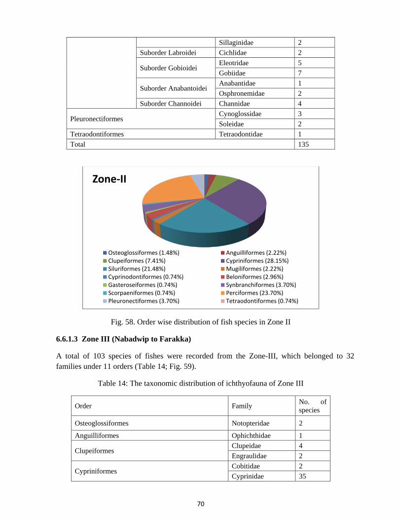
70
Sillaginidae 2 Suborder Labroidei Cichlidae 2
Suborder Gobioidei Eleotridae 5 Gobiidae 7
Suborder Anabantoidei Anabantidae 1 Osphronemidae 2
Suborder Channoidei Channidae 4
Pleuronectiformes Cynoglossidae 3 Soleidae 2
Tetraodontiformes Tetraodontidae 1 Total 135
Fig. 58. Order wise distribution of fish species in Zone II
6.6.1.3 Zone III (Nabadwip to Farakka)
A total of 103 species of fishes were recorded from the Zone-III, which belonged to 32 families under 11 orders (Table 14; Fig. 59).
Table 14: The taxonomic distribution of ichthyofauna of Zone III
Order Family No. of species
Osteoglossiformes Notopteridae 2
Anguilliformes Ophichthidae 1
Clupeiformes Clupeidae 4 Engraulidae 2
Cypriniformes Cobitidae 2 Cyprinidae 35
Zone-II
Osteoglossiformes (1.48%) Anguilliformes (2.22%)Clupeiformes (7.41%) Cypriniformes (28.15%)Siluriformes (21.48%) Mugiliformes (2.22%)Cyprinodontiformes (0.74%) Beloniformes (2.96%)Gasteroseiformes (0.74%) Synbranchiformes (3.70%)Scorpaeniformes (0.74%) Perciformes (23.70%)Pleuronectiformes (3.70%) Tetraodontiformes (0.74%)

71
Botiidae 2 Psilorhynchidae 1
Siluriformes
Bagridae 7 Clariidae 1 Erethistidae 1 Heteropneustidae 1 Pangasidae 1 Schilbeidae 6 Siluridae 4 Sisoridae 6
Mugiliformes Mugilidae 2 Cyprinodontiformes Aplocheilidae 1
Beloniformes Adrianichthyidae 1 Belonidae 1
Synbranchiformes Mastacembelidae 3 Synbranchidae 1
Perciformes
Suborder Percoidei
Ambassidae 3 Nandidae 1 Badidae 1 Sciaenidae 2
Suborder Labroidei Cichlidae 2 Suborder Gobioidei Gobiidae 1
Suborder Anabantoidei Anabantidae 1 Osphronemidae 2
Suborder Channoidei Channidae 4 Tetraodontiformes Tetraodontidae 1 Total 103
Fig. 59. Order wise distribution of fish species in Zone III
Zone-III
Osteoglossiformes (1.94%) Anguilliformes (0.97%)Clupeiformes (5.83%) Cypriniformes (38.83%)Siluriformes (26.21%) Mugiliformes (1.94%)Cyprinodontiformes (0.97%) Beloniformes (1.94%)Synbranchiformes (3.88%) Perciformes (16.50%)Tetraodontiformes (0.97%)

72
6.6.2 Diversity Indices
In order to get a measure of abundance and evenness of fish species distribution in the river stretch, different diversity indices were estimated such as Margalef’s species richness (d), Pielou's evenness (J'), Shannon H'(loge) and Simpson (1- Lambda) as shown in Fig. 60. Species richness is a measure for the total number of species in a community, whereas evenness expresses how evenly the individuals in a community are distributed among the different species.
Fig. 60. The diversity indices of various sampling stations (a)Shannon- Weiner index (b) Margalef’s species richness index (c) Pielou's evenness index and (d) Simpson index
The Shannon-Wiener index increased as both the richness and the evenness of the community increased. The stations Farakka, Nabadwip, Balagarh and Kakdwip (Ghoramara Island) showed high values for the index indicating rich fish diversity of the stretch. Farakka, the unloading point of the coal laden barges had maximum value for the index, indicating the biological significance and need to take precautions so as not to pollute this diverse stretch of Ganga. Pielou's evenness index (J') value was close to 1 for all stations indicating a very even distribution of abundance amongst all species. All the stations exhibited fair values for the indices indicating the healthy and diverse ecosystem of the river.
6.6.3 Species availability as per IUCN list
There are many species, which are listed in threatened and rare categories of IUCN (International Union for Conservation of Nature) red list among the species recorded in the stretch of River Ganga. As the IUCN Red List Index measures overall trends in extinction risk for groups of species based on genuine changes in their status over time, it provides a good indication of their conservation importance. Species such as Ailia coila, Anguilla bengalensis

73
bengalensis, Wallago attu, Ompok bimaculatus, O. pabda, and O. pabo are distributed well in the river stretch, they currently belong to the Near Threatened category in the IUCN red list. The species like Bagarius bagarius and B. yarrelli distributed in the Zone-III are also listed as Near Threatened in IUCN red list.
Studies indicated rich and diverse ichthyofauna of River Bhagirathi-Hooghly with unique and endemic species as well as species of high conservation needs. The river stretch is also the migratory route for many important species such as Tenualosa ilisha, contributing to the ecological importance of the river.
6.6.4 Probable impact of barge traffic on fishes
Fish can be negatively impacted by different kinds of vessel traffic including barges in a number of ways including:
(i) direct contact /collision leading to mortality,
(ii) pollutants and toxins from fuels and paints, and
(iii) increased sediments in the water column
(iv) constant stress, disturbance to breeding, feeding
As a vessel or barge navigates through a waterway, it generates hydraulic disturbances in the form of waves and currents, mainly drawdown, return current, slope supply currents, wash waves, and propeller jet. Thus, in addition to the indirect effects of “navigation” on fish assemblages, direct negative effects on fish caused by navigation induced shear stress, ship waves, drawdown, dewatering, backwash, and return currents have been commonly reported (Holland and Sylvester, 1983; Holland, 1986; Nielsen et al., 1986; Pygott et al., 1990; Odom et al., 1992; Zauner and Schiemer, 1992, 1994; Wolter and Vilcinskas, 1997; Jude et al., 1998; Killgore et al., 2001; Gutreuter et al., 2003), but rarely tested in situ (Mueller, 1980; Holland, 1986; Odom et al., 1992; Gutreuter et al., 2003) with partially contradictory results documenting impacts (Holland, 1986) or no impact (Odom et al., 1992). In general, it is often observed that commercial vessel traffic is negatively affecting native fish populations associated with channel bank habitats. As this pressure is expected to increase in the coming years, investigation on potential mitigation measures is desired.
Conducting a targeted complete impact assessment was not possible given the short span of the study period. However long term studies carried out elsewhere provide empirical evidence that intensive commercial navigation impairs fish assemblages in width-restricted waterways. These studies (Huckstorfet al., 2010; Husig et al., 2000) highlighted, in particular, those species that have their first nursery habitats in shoreline areas were more affected by intensive commercial navigation than species whose larvae live predominantly pelagic. The results indicated that the negative effect of intensive navigation on riverine fish results primarily from the navigation-induced hydraulic disturbances along the banks. Therefore, mitigation of navigation-induced hydraulic forces is required to prevent degradation of fish communities in waterways.

74
Slaberkoorn et al. (2010) called attention to a ‘noisy spring’, the possible detrimental impact of increasing levels of anthropogenic noise on fishes through a review article in line to Rachel Carson who wrote about a ‘silent spring’ in the context of the detrimental impact of the use of pesticides on singing birds in 1962. The underwater environment is filled with biotic and abiotic sounds, many of which can be important for the survival, communication or reproduction of fish. Over the last century, human activities in and near the water have increasingly added artificial sounds to this environment. Very loud sounds of relatively short exposure, such as those produced during pile driving, can harm nearby fish. However, more moderate underwater noises of longer duration, such as those produced by vessels and barges, could potentially impact much larger areas, and involve much larger numbers of fish. There is a need to study the role of sound in the lives of fish and to develop a better understanding of the ecological impact of anthropogenic noise.
6.6.4.1 Fish breeding
There are many studies on the impacts of vessels and barges on fish breeding. According to the Navigation-induced habitat bottleneck hypothesis (NBH concept), fish recruitment is limited because of a lack or restricted availability of essential nursery habitats resulting from navigation induced hydraulic forces that exceed the maximum swimming performance of fish (Wolter and Arlinghaus, 2003). Some studies reported that obstructing nest-guarding behaviour and dislodgement and redistribution of eggs into less suitable habitats lower the reproductive success of various fish species. Another major navigational impact reported is poor larval survival.
The period obtained for the field work was short with respect to study the impact of barge traffic on fish breeding since the breeding season varies for species to species. As per the situation, a small exploratory assessment was done to know the availability of fish spawn/ larvae along the study stretch using spawn collection nets during July, 2014 sampling. The cone shaped spawn collection nets were fixed against the water flow along the right and left edges of the shipping channel at each selected sampling site, for a duration of half an hour. The mass of spawn/larvae collected varied from site to site and were a mixture of different species of fishes distributed in the particular sites and the study indicated that fishes were breeding throughout the river stretch and the larvae and the spawns were abundant in the shipping channels too. The maximum fish spawn availability was noticed at Farakka followed by Triveni and Burul.
6.6.4.2 Fish migration
It is sometimes the case in fishes that the life history needs of a population (e.g., foraging and reproduction) cannot be met by a single habitat. This is due to variability in the habitat conditions (e.g., temperature), or to the changing needs of the population itself (e.g., foraging habitat vs. spawning habitat). In such cases, the fitness of individuals benefits from movement to an alternate habitat. As a result, many fishes have evolved a life history that includes coordinated movement from one habitat to another. This synchronous, directed movement of part or all of a population between discrete habitats is called ‘migration’. Approximately 2.5% of all fish species undertake migrations. Fish migrations are grouped into different categories
75
such as anadromous, catadromous, oceanodromous, and potamodromous etc., based on their relationship to the seawater /freshwater boundary.
6.6.4.2.1 Anadromous migration
Anadromy occurs when most feeding and growth occurs in saltwater and fully grown adults move back into freshwater to spawn. Among the fishes distributed in the studied stretch, the most important and well studied migratory species is Tenualosa ilisha, commonly called as hilsa shad. Belonging to family Clupeidae, the species inhabits rivers, estuaries and coastal waters. Hilsa spends its adult life in the marine environment and migrates to riverine habitats for breeding. The young ones migrate back to marine environment for growth. Due to its nutritional value and taste, the fish is considered a delicacy and provides direct or indirect livelihood to millions of fishers along the coastal and riverine stretches in its range of distribution. It is most abundant in the Ganga-Brahmaputra-Meghna river systems of India, Bangladesh and Myanmar, forming one of the most important commercial fisheries in these countries.
The species was earlier found to migrates up to Agra, Kanpur and Delhi in the years of excessive abundance, and up to Allahabad in normal years in the Ganga river system in the past (pre-Farakka barrage period). But after the construction of Farakka Barrage, the major population of the species was confined downstream of Farakka barrage. Hence the studied river stretch is the major area where the hilsa population migrate for breeding and the juveniles are grown till they return to the marine environment for reproductive growth. Recently, the Government of West Bengal, based on the recommendations provided by CIFRI, has issued gazette notification on 9th April 2013, attempting to conserve hilsa to facilitate their migration, breeding and growth; in which three hilsa sanctuaries are mentioned in the Hooghly-Bhagirathi river stretch- between Nishchintapur to Diamond Harbour (in between sampling sites Ghoramara Island and Roychak, channel chainage 40 to 70 km), between Hooghly Ghat to Kalna (in between sampling sites Triveni and Nabadwip, chainage 184 to 246 km) and between Lalbagh to Farakka (in between sampling sites Hotnagar and Farakka, chainage 442 to 540 km). These three suggested sanctuaries fall in the barge route under study. Hilsa have significant ecological, economic and cultural importance, and are currently the focus of conservation efforts to preserve the sustainability of the fisheries.
There are many others among the recorded species which shows anadromous migration, though not in a huge scale of distance as in case of T. ilisha. Stolephorus spp, the whitebaits are said to undergo anadromous migration from coastal waters to estuarine areas of rivers. Apart from fishes, there are many species of prawns distributed in the river Ganga which are migratory. Macrobrachium rosenbergii, the giant freshwater prawn, requires estuarine conditions for hatching and larval metamorphosis prior to upstream migration to freshwaters.
6.6.4.2.2 Catadromous migration
Catadromous fishes are ones that migrate from fresh water into the sea to spawn; or, ones that stay entirely in fresh water and migrate downstream to spawn. The species Anguilla bengalensis bengalensis, commonly called as Indian mottled eel, is a semelparous,

76
catadromous species. It is migratory, breeding in the ocean (Seegers et al. 2003) and migrating into freshwaters and estuaries, including large rivers, as juveniles (glass eels/elvers). Elvers can migrate high up rivers into streams where they inhabit pools until they mature although like many anguillid species some individuals will remain in coastal waters. Like other migratory species, its numbers and range have been reduced by dam building and other obstructions in their habitat. The species has been assessed as Near Threatened by IUCN; although there are no data available to determine actual rate of decline, it is suspected that a reduction of close to 30% is likely to have occurred over the last 3 decades, based on reports of declines across its range.
6.6.4.3 Amphidromous and potamodromous fishes
There are many amphidromous species among the ichthyofauna, which move from coastal to freshwater habitat and vice versa for feeding and other (not breeding) purposes. Amphidromous fishes that are spawned in freshwater, migrate downstream to the sea and then go upstream at a juvenile stage for further growth and reproduction. There are a large number of amphidromous species in the recorded ichthyofauna of the river stretch, the majority being recorded from the Zone-I and Zone-II as the influence of the coastal waters is more dominant in these zones. The species such as Eleutheronema tetradactylum, Polynemus paradiseus, Scatophagus argus, Liza spp etc. are significant among the amphidromous species distributed in the lower Ganga.
When fishes migrate from one freshwater habitat to another in search of food or for spawning, it is called potamodromous migration. There are about 8,000 known species that migrate within lakes and rivers, generally for food on daily basis as the availability of food differs from place to place and from season to season. Many species of fishes are potamodromous, which migrate within the river system. Potamodromous fish species are abundant in the River Ganga as the river has good flow and water availability throughout the year, the significant ones among the recorded ichthyofaunal of the river being Bagarius spp, Gagata spp, Eutropiichthys spp, Notopterus notopterus, Labeo spp, Catla catla etc.
Among all modes of transport, inland navigation with adopting proper procedures is currently considered the most environmentally sound and sustainable form (United Nations, 1997; Colvile et al., 2001; European Commission, 2001). According to a report by a sub group of the Working Group on Ports and Shipping under the National Transport Policy Development Committee (NTPDC) of the Planning Commission during 2012, a litre of diesel would carry 105 tonnes over a kilometre through waterways, 85 tonnes through railways and 24 tonnes through roadways (http://www.downtoearth.org.in/content/natural-highways?page=0,2). The emission of greenhouse gases is also relatively low from the sector. Conserving the ecological potential of fish communities in waterways or its sustainable management requires minimizing of navigation impacts through various methods such as by enhancing shoreline structures, ecotone diversity and enlargement or by revitalizing submerged and emerged macrophytes (Arlinghaus et al., 2002; Wolter, 2001).

77
6.7 Metal contaminations
Pollution is a common problem encountered in inland aquatic ecosystems and among the various pollutants, metals are of added concern due to their environmental persistence, biogeochemical recycling and ecological risks. The combined effect of the basin characteristics (relief, geology, climate, vegetation, size of the drainage area, etc.) and the anthropogenic activities (urban development, promotion of industries, mining, agriculture, deforestation etc.) govern the type, composition and quantity of metals accumulated and transported through the river. During premonsoon and monsoon study periods the content of five metals (Cadmium Cd, Copper Cu, Manganese Mn, Lead Pb and Zinc Zn) were recorded. Sample collection and analysis were based upon the methodology given in APHA (1995) for water and Hall (1997) for sediment samples. Water samples were concentrated 10 times during processing. Sediment samples were taken 1 g and final volume was 50 ml. The Instrument used was GBC AVANTA SIGMA in flame mode with minimum detection concentrations as: Cd 0.1 ppm; Cu 0.2 ppm; Mn 0.2 ppm; Pb 0.2 ppm and Zn 0.5 ppm. Since water was concentrated 10 times, the concentrations below one tenth of the mentioned concentrations have been mentioned as BDL (Below Detection Limit).
6.7.1 Water metal contaminations
For the total stretch, in most of the cases water metal content was recorded below the detection limit of the AAS. Only Mn, Cu and Zn were recorded in some cases and hence, water metal content was not a concern (Table 15). Although a significant stretch of the estuarine zone is densely industrialized and regularly receives effluents, the mixing and dilution with tidal water is maintaining the metal levels in water lower than that of the middle stretch (Vass et al., 2008). Elevated levels of water dissolved Hg, Ni, Pb and Zn were however, registered at the same time from the estuary (Kar, et al. 2008; Sarkar et al, 2007). In general, Ganga river water has alkaline pH, recorded range 7.0 – 9.2 (Vass et al., 2008) and in the present study 7.3 – 8.4. It facilitates metal ions to precipitate out on the sediment phase. Thus, the metals transported into the river system are retained mostly in the bottom sediments (Samanta, 2013).

78
Table 15. Concentration of trace metals in water (mg/l or ppm)
A) Premonsoon period
Sampling dates Cd Cu Mn Pb Zn
Farakka 1 26.3.14 BDL BDL BDL BDL BDL Farakka 2 26.3.14 BDL BDL BDL BDL BDL Jangipur 27.3.14 BDL BDL BDL BDL BDL Sundarpur Reach 27.3.14 BDL BDL BDL BDL BDL Hotnagar 28.3.14 BDL BDL BDL BDL BDL Plassey 28.3.14 BDL BDL BDL BDL BDL Katwa 29.3.14 BDL BDL BDL BDL BDL Nabadwip 30.3.14 BDL BDL 0.048 BDL BDL Balagarh 31.3.14 BDL BDL BDL BDL BDL Triveni 01.4.14 BDL BDL BDL BDL BDL Dakshineswar 03.4.14 BDL BDL 0.056 BDL BDL Burul 04.4.14 BDL BDL 0.142 BDL BDL Roychak 07.4.14 BDL BDL BDL BDL BDL Ghoramara Island 8.4.14 BDL BDL BDL BDL BDL
b) Monsoon period
Cd Cu Mn Pb Zn
Farakka 1 10.07.14 BDL 0.02 0.028 BDL 0.032 Farakka 2 10.07.14 BDL BDL BDL BDL 0.028 Jangipur 09.07.14 BDL BDL BDL BDL 0.039 Sundarpur Reach 11.07.14 BDL BDL BDL BDL BDL Hotnagar 12.07.14 BDL BDL BDL BDL BDL Plassey 16.07.14 BDL BDL BDL BDL BDL Katwa 17.07.14 BDL BDL BDL BDL BDL Nabadwip 17.07.14 BDL BDL 0.048 BDL BDL Balagarh 19.07.14 BDL BDL BDL BDL BDL Triveni 20.07.14 BDL BDL BDL BDL BDL Dakshineswar 14.07.14 BDL BDL 0.109 BDL BDL Uluberia 28.07.14 BDL BDL BDL BDL BDL Burul 30.07.14 BDL BDL BDL BDL BDL Roychak 29.07.14 BDL BDL BDL BDL BDL Ghoramara Island 31.07.14 BDL 0.044 0.039 BDL BDL

79
6.7.2 Sediment metal Contaminations
In sediments, dominance of Cu, Mn and Zn was recorded. Only Cu crossed marginally the non-pollutional limit of 25 mg/kg in the samples of Dakshineswar, Uluberia and Ghoramara island samples. In general, the studied metal contaminations in sediments were below the harmful levels (Table 16).
For study of metal contaminations in rivers, the water dissolved and sediment bound metals are routinely monitored. But the water dissolved metals are frequently transferred to the particulate state, adsorbed on the suspended sediments and carried with the moving phase. Such transportation of metals is very important especially in the estuarine stretch having different levels of tidal energy. An exhaustive study conducted by Mukherjee (2012) emphasized the role of suspended sediments for metal transportation in river Hooghly, the stretch having very high sediment load (annually 560 million tons) and strong tides, even up to 5.5 m. In the suspended sediments higher enrichment factor for Cu, Cd, Ni, Cr and Zn was recorded due to anthropogenic activities related to poor land uses for urbanization and industrialization. The waste water from the Kolkata city has also been proved as not been the major source of metal pollution of the river (Mukherjee, 2012). As a whole, the metal enrichment factors observed in river Hooghly was found relatively low compared to that reported for other rivers of the world (Samanta, 2013).
The Ganga Brahmaputra river system has very high sediment transportation load, amounting to 1620×106 ton annually, of which 1000×106 ton is carried as suspended load and 620× 106 ton as the bed-load. It has been observed that nearly 80% of bed load sediments are moved as “graded suspension” during the monsoon season. Thus, the river bed is flushed during every monsoon, preventing higher accumulation of toxic contaminants.
The coal samples obtained as contaminants in the sediments at the coal unloading site of Farakka 2 sampling site during initial sampling were also analyzed for metal contaminations. It was found free from Cd, Cu and Pb. Mn was detected at 429 ppm and Zn 41.8 ppm. Zn content was below the pollutional level for sediments (90 ppm).

80
Table 16.Concentration of trace metals in sediments (mg/kg sediment or ppm)
A. Premonsoon
Cd Cu Mn Pb Zn
Farakka 1 26.3.14 BDL 9.236 28.857 BDL 49.044 Farakka 2 26.3.14 BDL 16.88 77.490 BDL 41.294 Jangipur 27.3.14 BDL BDL 152.168 BDL BDL Sundarpur Reach 27.3.14 BDL 19.027 44.306 BDL 43.397 Hotnagar 28.3.14 BDL 9.705 43.472 BDL 44.013 Plassey 28.3.14 BDL 13.429 BDL BDL 37.348 Katwa 29.3.14 BDL BDL 119.426 BDL BDL Nabadwip 30.3.14 BDL 8.269 69.169 BDL 32.586 Balagarh 31.3.14 BDL BDL 108.615 BDL BDL Triveni 01.4.14 BDL 17.346 65.500 BDL 48.989 Dakshineswar 03.4.14 BDL 27.838 91.713 BDL 60.583 Burul 04.4.14 BDL 21.615 101.182 BDL 59.006 Roychak 07.4.14 BDL 19.942 102.797 BDL 54.907 Ghoramara Island 08.4.14 BDL 25.373 110.649 BDL 65.441
B. Monsoon
Cd Cu Mn Pb Zn
Farakka 1 10.07.14 BDL BDL 170.428 BDL 16.39 Farakka 2 10.07.14 BDL 22.446 264.968 BDL 54.362 Jangipur 09.07.14 BDL BDL 155.505 BDL 13.966 Sundarpur Reach 11.07.14 BDL 6.701 148.437 BDL 20.246 Hotnagar 12.07.14 BDL 15.579 219.860 BDL 39.92 Plassey 16.07.14 BDL BDL 215.203 BDL 38.911 Katwa 17.07.14 BDL BDL 152.560 BDL 24.524 Nabadwip 17.07.14 BDL BDL 159.638 BDL 26.889 Balagarh 19.07.14 BDL 22.744 314.250 BDL 62.898 Triveni 20.07.14 BDL 20.377 433.880 BDL 58.363 Dakshineswar 14.07.14 BDL 30.677 705.110 BDL 73.473 Uluberia 28.07.14 BDL 25.99 573.370 BDL 76.977 Burul 30.07.14 BDL BDL 319.220 BDL 45.426 Roychak 29.07.14 BDL 14.128 398.375 BDL 44.416 Ghoramara Island 31.07.14 BDL 19.656 471.090 BDL BDL Coal (From Sediment)
BDL BDL 428.850 BDL 41.798

81
6.8 Socio-economic study
The Bhagirathi-Hooghly river stretch although was designated during 1986 as part of NW-I, only the Triveni to Sagar stretch was in use so far for navigation. In the Farakka to Triveni stretch since the water traffic was less, the local fishers were utilizing the resource for their lively hood. But when the movement of coal bearing barges started, the fishers have limits to utilize the navigation channel area during the physical movement of the barges. Thus, it is anticipated that the fishers are affected in this fresh initiatives. To see if the barge movement has any impact on fishing activity and fishers livelihoods, a targeted study was conducted. The details of the study are as following.
6.8.1 Sampling plan A sizeable population of fishers depends on the Bhagirathi-Hooghly stretch of river for their daily livelihoods and fishing has been the main contributor of their total income. Any disturbance including movement of vessels in the river will have direct bearing on the fishing operations. For the present study, the entire stretch from Sagar Island to Farakka was divided into three zones depending upon the frequency of movement of the ship and other merchant vessel. The first zone (Zone I, lower zone) is from Sagar Island to Baranagar (near Dakshineswar) which is 154 km in length. The second zone (Zone II, middle zone) is from Baranagar to Dampal Char/Naupara crossing (25 km above Nabadwip) which is also 154 km in length. The last zone (upper zone) is up to Farakka NTPC point which is 237 km long. In the first zone the vessel movement is more frequent because regular vessel comes to the Kolkata/Kidderpore dock. In the second zone the vessel movement is much less. Third zone is the least disturbed as far as movement of vessel is concerned. For socio-economic impact study 19 sampling sites have been identified, 7 from lower zone; 6 from middle zone and 6 from upper zone. The detail of the sampling sites has been given in Table 17.
Table 17. Sampling sites
Zone Distance (km)
No. of sampling sites
Sites
I Lower Zone 0 – 154 7 Sagar light house, Maya Goyalini Ghat/Rudra Nagar, Ghoramara Island, Diamond Harbour, Nurpur/Roychak, Uluberia, Baranagar (near Dakshineswar)
II Middle Zone
154 – 308
6 Barrackpore/Nawabganj/Debitala, Hooghly ghat/Triveni, Balagarh, Ambika Kalna, Nabadwip/Kharer Math and Dampal Char/Naupara crossing/Jhasudanga
III Upper Zone 308 – 545
6 Katwa, Chowrigachha, Lalbagh, Jangipur, Putimari and Farakka
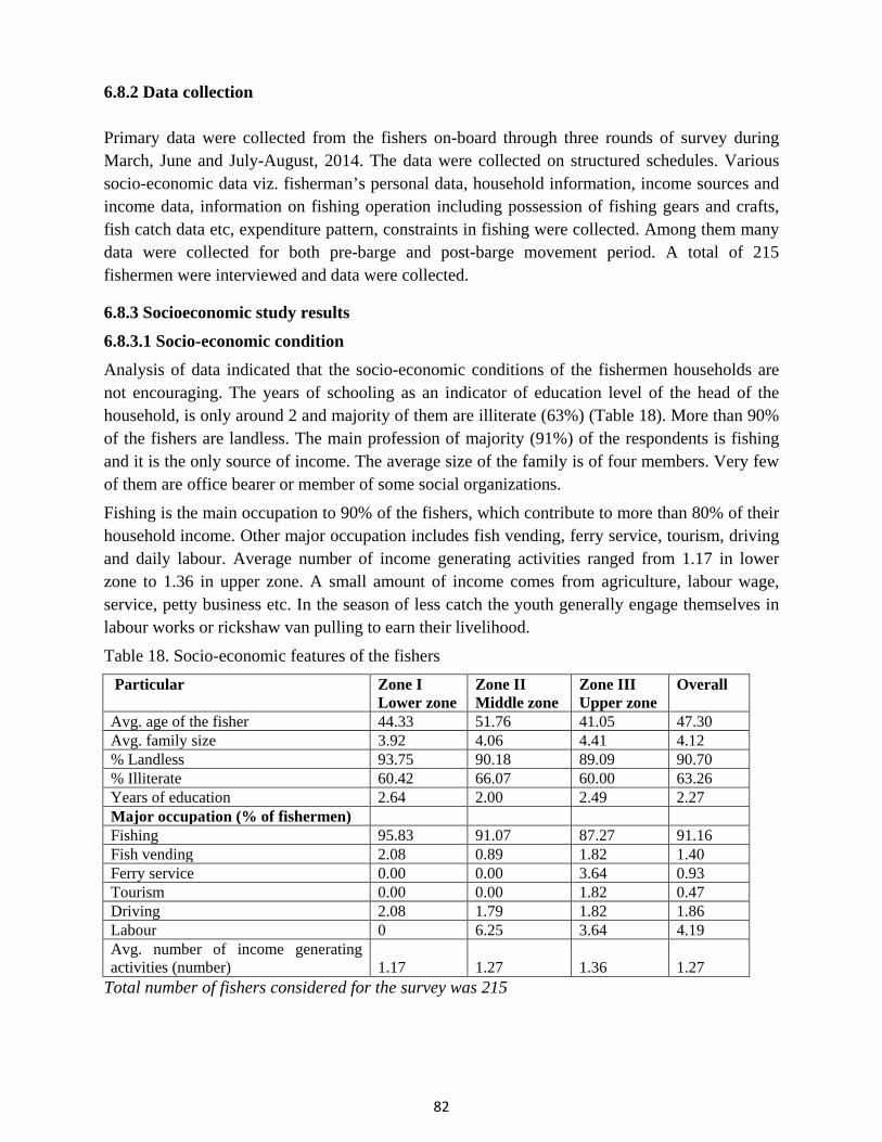
82
6.8.2 Data collection Primary data were collected from the fishers on-board through three rounds of survey during March, June and July-August, 2014. The data were collected on structured schedules. Various socio-economic data viz. fisherman’s personal data, household information, income sources and income data, information on fishing operation including possession of fishing gears and crafts, fish catch data etc, expenditure pattern, constraints in fishing were collected. Among them many data were collected for both pre-barge and post-barge movement period. A total of 215 fishermen were interviewed and data were collected.
6.8.3 Socioeconomic study results 6.8.3.1 Socio-economic condition Analysis of data indicated that the socio-economic conditions of the fishermen households are not encouraging. The years of schooling as an indicator of education level of the head of the household, is only around 2 and majority of them are illiterate (63%) (Table 18). More than 90% of the fishers are landless. The main profession of majority (91%) of the respondents is fishing and it is the only source of income. The average size of the family is of four members. Very few of them are office bearer or member of some social organizations. Fishing is the main occupation to 90% of the fishers, which contribute to more than 80% of their household income. Other major occupation includes fish vending, ferry service, tourism, driving and daily labour. Average number of income generating activities ranged from 1.17 in lower zone to 1.36 in upper zone. A small amount of income comes from agriculture, labour wage, service, petty business etc. In the season of less catch the youth generally engage themselves in labour works or rickshaw van pulling to earn their livelihood.
Table 18. Socio-economic features of the fishers Particular Zone I
Lower zone Zone II Middle zone
Zone III Upper zone
Overall
Avg. age of the fisher 44.33 51.76 41.05 47.30 Avg. family size 3.92 4.06 4.41 4.12 % Landless 93.75 90.18 89.09 90.70 % Illiterate 60.42 66.07 60.00 63.26 Years of education 2.64 2.00 2.49 2.27 Major occupation (% of fishermen)
Fishing 95.83 91.07 87.27 91.16 Fish vending 2.08 0.89 1.82 1.40 Ferry service 0.00 0.00 3.64 0.93 Tourism 0.00 0.00 1.82 0.47 Driving 2.08 1.79 1.82 1.86 Labour 0 6.25 3.64 4.19 Avg. number of income generating activities (number) 1.17 1.27 1.36 1.27
Total number of fishers considered for the survey was 215

83
Food75%
Others25%
Fuel6% Clothing
17%Medical
12%
Entertainment1%Utilities
5%HH items6%
Social obligations
6%
Education21%
Others26%
Food79%
Others21%
Fuel1%
Clothing27%
Medical10%
Entertainment3%Utilities
8%HH items
8%
Social obligations
4%
Education15%
Others24%
Food77%
Others23%
Fuel4%
Clothing19%
Medical9%
Entertainment4%
Utilities7%HH items
9%
Social obligations
8%
Education11%
Others29%
6.8.3.2 Income-expenditure pattern
Fig. 61. Items of monthly expenditure (Rs.7846.23) in Upper Zone (III) Total Monthly income Rs.7916.73
Fig. 62. Items of monthly expenditure (Rs.7095.21) in MiddleZone (II) Monthly income Rs.8446.07
Fig. 63. Items of monthly expenditure (Rs.8014.29) in Lower Zone (I) Total monthly income Rs. 10247.23

84
Fuel3%
Clothing22% Medical
10%
Entertainment2%
Utilities7%
HH items8%
Social obligations
6%
Education16%
Others26%
Food78%
Others
22%
Fig. 64. Items of monthly expenditure (Rs.7488.11) for Overall Total monthly income Rs. 8705.61 The monthly income of the household ranged from Rs.7,917 in zone III (upper zone) to Rs.10,247 in zone I (lower zone), the average being Rs.8,706 (Fig. 61 to 64). The income is higher in lower zone because of higher catch and high value fish (mainly hilsa) in the catch. The household spent on an average Rs.7,500 on different items per month. The food expenditure took around 78% of the total expenses. Other major items of expenditure are clothing (5%), medical (3%) and household items (2%), education (3.5%) and others (6%). The barge movement for carrying coal was during October 2013 to May, 2014. So far, it does not have any impact on the expenditure pattern of the fisherman household across the zones.
Various forms of gill nets and bag nets are found to be operated by the fishers. Among them gill nets are most prevalent throughout the stretch. Around 80% of the fishers were using the gear (Table 19). The gill nets have different local names like Current jal, Nagin jal, Kajli jal, Phasa jal, Bhola jal, Vacha jal, Ghero jal, Dhoali jal, Gule jal, Pungus jal,etc. A number of variations in material and mesh size in gill nets are observed depending upon the targeted fishes. However, drift gill nets are the major nets used to catch hilsa, the main migratory fish of Bhagirathi- Hooghly river system. All different types of gill nets have their distinct seasonality in operation depending upon the availability of the target species.

85
Table 19. Fishing gears and crafts being operated (% of fishermen)
Gear/net Zone I Lower Zone
Zone II Middle Zone
Zone III Upper Zone Overall
Gill net 79.17 82.14 80.00 78.60 Hook and line 10.42 7.14 3.64 6.98 Dragnet 2.08 - 1.82 0.93 Bag net 20.83 16.07 - 13.02 Cast net 4.17 10.71 7.27 8.37 Trawl nets 2.08 8.93 - 5.12 Meen jal 16.67 1.79 - 4.65 Set barrier 6.25 1.79 - 2.33 Trap 2.08 10.71 16.36 10.23 Lift net (vasal) 2.08 5.36 5.45 4.65 Crafts
Dingi 8.33 8.04 58.18 20.93 Boat 75.00 95.54 38.18 76.28 No. of family member fish 1.08 3.76 1.47 1.37
Bag nets are mostly used in the lower zone. Bag net operation generally remains suspended during monsoon months of July-October at most of the places because of high water current. Bag nets are mostly set at bottom using PVC / Thermocol float, however surface set bag net are observed in some areas. Charpata jal is observed in lower zone. Trawl nets are used to fish prawns. Lift nets (Vessal) is operated at near-shore region as well as from boats. Cast nets could be found in the entire stretch of the river. Meen jal, meant to collect fish and prawn larvae to be used for stocking in aquaculture ponds. Hook and line is another gear which is used everywhere. Various types of baits like wheat ball, earthworm, prawn, insect larvae and egg etc. are used as bait in hook and line. Various types of traps are also observed to be used particularly in the upper zone. Single piece tin made fishing craft dingi are mostly found in upper and middle zone, whereas the wooden boats are mostly found in the lower zone.
Fishers’ perception on impact of barge movement
6.8.3.3 Perception on impact of barge movement on ecology
The fishers were asked to record their views on the visible impact of barge movement on ecology and environment. The response has been presented in Table 20. Some of the fishers of upper and middle zones (II and III) narrated the soil erosion problem. At this stretch the river is narrower and the wave created by the movement of barge cause soil erosion of the banks. In the lower zone it is not a problem as the river is wide enough to subside the wave strength by the time it reach the banks. Majority of the lower zone fishers did not express any visible impact.

86
Table 20. Views of the fishers (%) on visible impact on ecology (%)
Particular Zone I Lower Zone
Zone II Middle Zone
Zone III Upper Zone Overall
Can’t say 14.58 26.79 56.36 31.63 Soil erosion 0.00 18.75 27.27 16.74 Increased turbidity 0.00 0.89 1.82 0.93 Aquatic plants destruction 0.00 0.00 1.82 0.47 Nil impact 85.42 55.36 12.73 51.16
Total number of fishers considered for the survey was 215
6.8.3.4 Fishers’ perception on impact of barge movement on fisheries
Table 21. Impact on fisheries (% of fishers)
Particular Zone I Lower Zone
Zone II Middle Zone
Zone III Upper Zone Overall
Destruction of nets 2.08 7.14 9.09 6.51 Boat sinks 0.00 0.89 1.82 0.93 Less fish catch 2.08 8.04 5.45 6.05 No impact on fish catch 91.67 93.75 87.27 91.63 Avg. fishing time lost (minute) 12.77 34.87 38.45 30.01
Total number of fishers considered for the survey was 215
Generally one member of the family is engaged in fishing, sometimes two, the average comes out to be 1.24. The fishermen do fishing for 5-12 hours daily, depending upon the season. Although majority of the fishers (91%) told that the barge movement does not have any impact on fish catch it has some impact on their fishing hours (Table 21). Both the barge movement and fishing activity depend upon the tidal activity, particularly in the middle and lower stretches. Fishermen have to terminate the fishing activity and wind up the nets when vessel comes. The fishermen reported that sometimes 5-6 vessels come in a row. The vessel itself and the subsequent waves created by the vessels disturbed the fishing activity. On an average, the vessel movement causes 20 to 30 minutes disturbances to fishing activities when the barges move. The extent of disturbance is higher in upper zone. However, the barge movement, as such, doesn’t have any impact on type of crafts and gears used, number of family members involved and species caught till now.
Some cases of destruction of nets have been reported particularly from upper and middle zones. As a result of which few farmers reported that they faced hardships in fishing. Keeping in view the socio-economic condition and fishery being the major contributor of their family income, the destruction of nets would have significant impact on their livelihood of the fishermen. The observation revealed that the impact on fishing was restricted to the upper and middle zones only. However, till date the change in occupation or incidence of leaving fishing operations are not reported. In the lower zone (Zone I) particularly from Nurpur/Roychak to Sagar the barge movement does not have any significant impact on fisheries. At this stretch the river is wide

87
enough and the route is busy even otherwise for vessel movement. Hence, fishermen were habituated with the vessel movement.
6.8.3.5 Fishers’ perception on long term impact of barge movement
Table 22. Fisher’s perception on long-term impact of barge movement (% of fishers)
Particular Zone I Lower Zone
Zone II Middle zone
Zone III Upper zone Overall
Loss of Agricultural land 2.08 8.93 14.55 8.84 Reduction of fish stock 2.08 1.79 - 2.33 Livelihood at risk 4.17 13.39 21.82 13.49 Change the profession - 3.57 3.64 2.79 No impact 62.50 35.71 27.27 39.53 Don't know 31.25 41.07 32.73 36.74
Total number of fishers considered for the survey was 215
Fishermen along the river have serious concerns that if the barge movement continues for long there might be several impacts on them as given in Table 22. The loss in agricultural lands will be due to breaking of embankments as a result of waves caused by barge movement.
6.8.3.6 Constraints reported by the fishers due to barge movement
Table 23. Type of constraints reported by the fishers due to barge movement (% of fishers)
Constraints Zone I Lower Zone
Zone II Middle Zone
Zone III Upper Zone
Overall
Have to suspends the fishing operation when barge comes - 30.36 43.64 26.98 Net dislodged due to heavy wave 6.25 23.21 30.91 21.40 Less concentration on fishing 4.17 27.68 32.73 23.72 Loss of fishing time 4.17 27.68 38.18 25.12 Chance of net damage 2.08 16.07 16.36 13.02 Chance of accident - 7.14 10.91 6.51 Barge anchors at fishing areas 2.08 - - 0.47 Nil 79.17 25.00 20.00 35.81
Total number of fishers considered for the survey was 215
Fishers reported many constraints which were grouped into 8 categories (Table 23). The constraints were more pronounced at upper and middle zones. The major constraints are interruption of fishing operations, dislodging of nets, loss of fishing time and chances of net damage. Loss of fishing times happens due to coincidence of barge movement and fishing activities, as both depends on tides in the lower stretch. Some fishers also reported about chances of net damage.
6.8.3.7 Suggestions prescribed by the fishers
An attempt was made to bring out the suggestions prescribed by the fishers. The table 24 shows that fishers revealed a number of suggestions. Among them some are quite good and feasible.

88
Pre-announcement of the time schedule, speed control, bright light and horn, move only through the designated channel were the major suggestions which a number of fishers opined. Quick compensation in case of damage of nets and boats are other important suggestions. Another two suggestion, barge may avoid the tidal time and concretize the banks are non-feasible suggestions. 81% of the lower zone fishers didn’t have any suggestions, which may be due to fewer problems faced by them.
Table.24. Suggestions prescribed by the fishers (% of fishers)
Suggestion Zone I Lower Zone
Zone II Middle zone
Zone III Upper zone Overall
Can't say/No suggestions 81.25 24.11 37.50 33.49 Speed control - 28.57 43.64 26.05 Bright light and horn 10.42 34.82 47.27 32.56 Announcement of time schedule 6.25 16.96 25.45 16.74 To move in channel only 6.25 8.93 12.73 9.30 Barge may avoid the tidal time - 12.50 9.09 8.84 Concrete the banks - 1.79 5.45 2.33 Compensation 6.25 20.54 36.36 21.40 Total number of fishers considered for the survey was 215
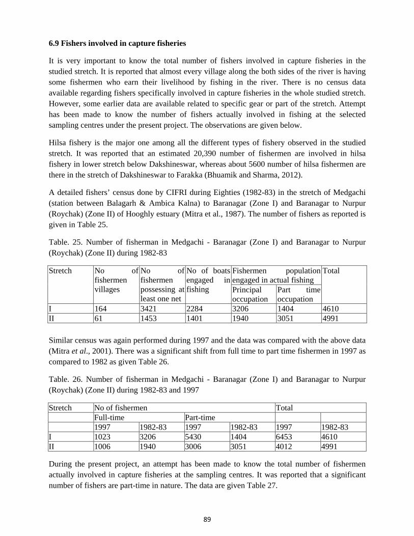
89
6.9 Fishers involved in capture fisheries
It is very important to know the total number of fishers involved in capture fisheries in the studied stretch. It is reported that almost every village along the both sides of the river is having some fishermen who earn their livelihood by fishing in the river. There is no census data available regarding fishers specifically involved in capture fisheries in the whole studied stretch. However, some earlier data are available related to specific gear or part of the stretch. Attempt has been made to know the number of fishers actually involved in fishing at the selected sampling centres under the present project. The observations are given below.
Hilsa fishery is the major one among all the different types of fishery observed in the studied stretch. It was reported that an estimated 20,390 number of fishermen are involved in hilsa fishery in lower stretch below Dakshineswar, whereas about 5600 number of hilsa fishermen are there in the stretch of Dakshineswar to Farakka (Bhuamik and Sharma, 2012).
A detailed fishers’ census done by CIFRI during Eighties (1982-83) in the stretch of Medgachi (station between Balagarh & Ambica Kalna) to Baranagar (Zone I) and Baranagar to Nurpur (Roychak) (Zone II) of Hooghly estuary (Mitra et al., 1987). The number of fishers as reported is given in Table 25.
Table. 25. Number of fisherman in Medgachi - Baranagar (Zone I) and Baranagar to Nurpur (Roychak) (Zone II) during 1982-83
Stretch No of fishermen villages
No of fishermen possessing at least one net
No of boats engaged in fishing
Fishermen population engaged in actual fishing
Total
Principal occupation
Part time occupation
I 164 3421 2284 3206 1404 4610 II 61 1453 1401 1940 3051 4991
Similar census was again performed during 1997 and the data was compared with the above data (Mitra et al., 2001). There was a significant shift from full time to part time fishermen in 1997 as compared to 1982 as given Table 26.
Table. 26. Number of fisherman in Medgachi - Baranagar (Zone I) and Baranagar to Nurpur (Roychak) (Zone II) during 1982-83 and 1997
Stretch No of fishermen Total Full-time Part-time 1997 1982-83 1997 1982-83 1997 1982-83 I 1023 3206 5430 1404 6453 4610 II 1006 1940 3006 3051 4012 4991
During the present project, an attempt has been made to know the total number of fishermen actually involved in capture fisheries at the sampling centres. It was reported that a significant number of fishers are part-time in nature. The data are given Table 27.

90
Table 27. Number of fishers at the sampling centres
Sl. No. Station No of fishermen 1. Farakka 60 2. Dhulian 3 3. Jangipur 40 4. Sundarpur 5 5. Lalbagh 60 6. Hotnagar 20 7. Chowrigacha 35 8. Plassey 6 9. Katwa 35 10. Pakhichar 35 11. Prachin Mayapur 250 12. Jhasudanga 15 13. Nabadwip 95 14. Ambica Kalna 300 (35 full-time) 15. Balagarh 300 (35 full-time) 16. Triveni (Netaji
Colony) 35
17. Hooghly Ghat 100 18. Bichalighat 30 19. Nawabganj-
Debitala 35
20. Baranagar-Bally 30 21. Uluberia 15 22. Burul 45 23. Roychak 6 24. Ghoramara Island 8 25. Mayagoalini Ghat 5
(The numbers are approximate and as per the data collected through surveys during sampling)

91
6.10 Major fishing gears in operation
Since fishers are facing difficulty in operation of some of the fishing nets under present circumstances, effort were made to record the details of fishing nets and gears which are in use. The data will serve as the base line for understanding impact of barge movement on fishing operations. Major fishing gears involved in capture fishery in the Bhagirathi-Hooghly river stretch are the various forms of gill net and bag net. On an average, bag nets contribute 73% whereas drift gill net contribute 24% of the total fish catch in Hooghly estuary (Mitra et al., 2001). The rest of the gears catch about only 3% of the total catch. Lot of variations in material and mesh size in drift gill net is observed depending upon the target fishes. However, the major drift gill net is the nets used to catch hilsa, the main migratory fish of Bhagirathi-Hooghly river system. Though the recommended mesh size for hilsa is >90 mm to avoid catch of smaller hilsa (<500 gm), net with smaller mesh size of 55-80 mm is quite rampant especially during winter migration of hilsa. Even 14-26 mm mesh size drift gill nets are used to catch juvenile hilsa (10-30 gm) during their return journey to sea especially during the months of March-May. Various forms of drift gill net and bag net and their distribution in selected stations are given in Table 28. Distribution of other minor fishing gears is given in Table 29. All different types of gill nets have their distinct seasonality depending upon the availability of the target species. Monofilament drift gill net (locally called current jal / chhandi jal) of different mesh size targeted for hilsa mainly operated during monsoon months (July-October) and winter months (February-March) to catch them during migration. Fishers use different mesh size net piece to assemble together to make a long drift gill net. Width of the net varies widely ranging from 9-45 ft. However, length of drift gill net increases as width of the river increases. At Lalbagh, in tin-made dingi boats only one piece of net (approx. 100 ft long) is used whereas in large wooden boats 3 pieces are used to cover the whole river there. At Dakshineswar, 6 such pieces are added to have a length of approx. 750 ft. At Godakhali (between Uluberia and Burul), length of hilsa net is approx. 1800 ft, which increases to approx. 8400 ft at Nischintapur region (above Ghoramara Island). In some places, those nets are operated even during non-migration period as some hilsa are available throughout the year. At Nischintapur, drift gill net are set both at surface or bottom using proper floats. As expected, bottom set drift gill net drifts less with time, but catch is more in surface set gill net. Nets with bigger mesh size (locally called cot jal made of parachute wire; 5-9” mesh size) are operated in entire stretch of the river to catch large fishes. At Chowrigacha (near Hotnagar), cot jal catch includes Catla catla, Pangasius pangasius etc. At Diamond Harbour (below Roychak), such nets are called as Pangas jal (as it catches Pangasius pangasius). At still lower stretch, 9” mesh Sele jal is used during winter months (named such as its catch includes large sele fish, Polydactylus indicus). Other targeted drift gill net like Bhola jal (42, 44, 46, 48 mm mesh gill net) to catch sciaenids like Otolithoides pama is operated in lower estuary mainly during the months of September-November. Topsey jal (26, 28 mm mesh net targeting Polynemus paradiseus) is used during the months of February-June. Vacha / Gorcha/ Ghero / Ghoura jal with 1” mesh size gill net targeting Eutropichthys vacha, Clepisoma garua etc. are

92
operated at different stations from Farakka to Triveni. All selective gill nets are observed to catch some other fishes with similar dorso-ventral length. Piuli jal (14 mm mesh) meant for Aspidoparia morar are also observed to catch small hilsa juveniles in upper Hooghly estuary and Bhagirathi river. Similar mesh size net, Chela jal was observed to be operated in upper estuary. Bhola / Topsey jal catch in lower estuary also have minor contribution from Sillago sp., Setipinna phasa, Eleutheronema tetradactylum etc. and even small size hilsa. Similarly, Hilsa jal catch in middle estuary observed to include C. garua, S. phasa etc. In lower estuary, tidal and lunar cycle used to influence catch of both gill net and bag net. For example, in September, same fisher at Diamond Harbour was observed to use hilsa jal during days around full / new moon (Bhora kotal) whereas during other days when flow is less (mora kotal) operates bhola jal. Similar to current jal, gill net made with nylon are used to catch other fishes especially near shoreline areas. Various other forms of drift gill nets with different mesh size like Nagin jal, Kajli jal, Phasa jal, Dholi jal, Gule jal are used in different regions targeting various fishes with higher abundance. Nagin jal, Kajli jal, Vacha jal, Ghero jal are almost similar type gill net with slightly local variation. At Prachin Mayapur (Nabadwip area), Dholi jal catch included Tulbele (Sillago panijus), Tengra (Mystus sp.) etc. Patan jal is a set gill net observed to be used in some places like Balagarh. Kona jal, though previously reported as gill net, is observed to catch fishes by trapping them in pockets near sinker.
Bag net operation generally remains suspended during monsoon months of July-October at most of the places because anchoring rope of bag net creates problem for drifting of gill net targeting hilsa. Bag nets are not used during full/new moon days due to heavy water current in lower estuary like Nischintapur, Diamond Harbour, etc. whereas in upper estuary from Triveni to Godakhali, catch is more during those full/new moon days. Bag net catch used to increase from upper to lower estuary. On an average, 15-20 kg catch was observed per bag net operation at Nischintapur. Bag nets are mostly set at bottom using PVC / Thermocol float, however surface set bag net are observed in some areas like Godakhali.

93
Table 28. Distribution (number) of gill net and bag net in selected centres of river Bhagirathi-Hooghly Gill net (4-
9”) (Cot/ Phans / Pangas / Sele/Nakurey jal)
Gill net (Chhandi/ current jal) (40-110 mm)
Nylon jal (3", 4")
Nagin jal (1”)
Phasa jal (2")
Bhola jal (42, 44, 46 mm)
Topse jal (26, 28 mm)
Kajli jal
Dholi jal (1, 1.5")
Kona jal (1.5-3.0")
Vacha / Gorcha jal(1.5”)
Piuli jal (14 mm)
Chela jal (20 mm)
Gule jal
Patang jal (set gill net)
Dubo beenti
Bhasa beenti
Fig. 66 Fig. 65 Fig. 67 Fig. 68 Fig. 69
Fig. 70
Fig. 71
Fig. 72 Fig. 73
Fig.74
1. Farakka 14 100 100 10 30 100 10-12 4 2. Jangipur 12 25 12 35 5 3. Dhulian
(Puthimari) 6
4. Sundarpur Reach
1
5. Lalbagh 110 50 40 50 20 6. Hotnagar 35 4 7. Chowrigach
a 30 30
8. Plassey 5 9. Katwa 8 15 10. Pakhichar 6 23 11. Prachin
Mayapur 95
12. Jhasudanga 8 13. Nabadwip 5 33 20 100 14. Ambica
Kalna 15 50
15. Balagarh 25 60 2 16. Triveni 47 16 17. Hooghlygha
t 50 20 12 6
18. Bichalighat 2 40 5 19. Nawabganj-
Debitala 8 70
20. Bally/ Baranagar
34 6
21. Uluberia 25 22 22. Godakhali 100 30-40 23. Burul 30 18 7 24. Roychak 34 25. Diamond
Harbour 20-25 32 32 18-20
26. Nischintapur
400 11
27. Ghoramara island
8
28.
Maya Goalini Ghat
5
(The numbers are approximate and as per the data received during sampling)
Fig. 65. Current jal with hilsa catch Fig. 66. Sele jal to catch large fishes

94
Fig. 67. Bhola jal along with its catch at D. Harbour
Fig. 68. Topse jal targeting Topsey (Polynemus paradiseus)
Fig. 69. Kona jal operation in Farakka Fig. 70. Vacha / Ghoura jal with its catch of
Clupesoma garua&Eutropichthys vacha
Fig. 71. Small mesh gill net responsible for catch of hilsa juvenile (10-20 gm)
Fig. 72. Chela jal, small mesh gill net targeting Chela / Salmostoma sp.
Fig. 73. Dubo Beenti - bottom set bag net, the main fishing gear of Hooghly estuary
Fig. 74. Bhasa beenti, surface set bag net operated at middle Hooghly estuary

95
Other fishing gears
There are various other types of fishing gears used by fishers to catch fishes from all ecological niches. Sanglo jal, a purse net / clap net targeting only hilsa is operated in middle estuary. Ber jal, seine net is observed to be used in upper estuary in all the seasons, but relatively less in monsoon due to high volume of water. Charpata jal, set barrier net is used taking the advantage of water level fluctuation with tidal cycle. Very long charpata jal is observed in lower estuary. It is less used during summer for storm (Kalboisakhi) and monsoon due to very high water level. Katal, a fish aggregating device using floating water hyacinth is less in the main channel due to high water current. It is observed at the confluence of Jalangi river with Bhagirathi at Nabadwip. Moi jal, Katni jal etc. are trawl nets used in bottom to catch prawns in upper estuary. Genra vessal is fixed lift net operated near-shore region operated in upper Hooghly estuary and Bhagirathi river. Nouka vessal is the mobile version of Genra vessal is operated from boat. Seitki jal is another form of lift net used in upper estuary. Khepla jal / Bachari jal is the cast net omnipresent throughout the entire stretch of the river. Meen jal, meant to collect fish and prawn larvae to be used for stocking in captivity is used at most of the stations especially during April to August. However, its shape, size, mode of operation varied widely from place to place depending upon terrain near shoreline. Hook & line is another gear which is used everywhere. Various types of bait like wheat ball, earthworm, prawn, insect larvae and egg etc are used as bait in hook & line. Multiple hooks from same line are operated from boat whereas single hook is operated from shoreline. At Diamond Harbour, hook and line catch includes fish species like Pangasius pangasius, Mystus gulio, Arius sp., Cephalocassis jatia, etc. At Triveni region, hook & line catch mostly consisted of Clupesoma garua and Eutropichthys vacha. Various types of traps are observed to be used especially in Bhagirathi river and upper Hooghly estuary.

96
Table 29. Distribution of other fishing gear in lower stretch of river Bhagirathi-Hooghly Sanglo
jal Ber jal Charpa
ta Katal (FAD)
Moi jal Katni jal
Thopa jal
Genra vessal
Nouka vessal
Seitki jal
Khepla jal
Meen jal
Hook & line (multiple)
Trap (small) (Bitti/Dhol)
Trap (Big) (Duar)
Trap (net made duar)
Trap (Net made)
Fig. 75 Fig. 76 Fig. 77 Fig. 78 Fig. 79 Fig. 80 Fig. 81 Fig. 82 Fig. 83 Fig. 84 Fig. 85 Fig. 86 Fig. 87 Fig. 88 1 Farakka 8 1 40 20-25 Tubey Sabar
jal 20
2.
Jangipur/Raghunathganj
3 7 50
3. Dhulian (Puthimari)
4. Sundarpur Reach
5 60
5. Lalbagh 15 20 30 400 500 6. Hotnagar 3 225 7. Chowrigacha 20 70 10 8. Plassey 6 1 1 9. Katwa 1 4 12 10. Pakhichar 10 5 4 320 11. PrachinMaya
pur 20
12. Jhasudanga 12 450 4 13. Nabadwip 2 2 20 17 6 70 20 15 14. Ambica
Kalna 2 60 40 60
15. Balagarh 10 4 10 12 175 16. Triveni 7 5 8 15 12 100 17. Hooghlyghat 5 10 40 18. Bichalighat 5 15 3 19. Nawabganj-
Debitala 3 15 2 4
20. Bally/ Baranagar
8
21. Uluberia 12 15 22. Godakhali 2-6 23. Burul 100 24. Roychak 3 2 45 25. Diamond
Harbour
7
26. Nischintapur 27. Ghoramara
island
28. Maya Goalini Ghat
(The numbers are approximate and as per the data received during sampling)
Fig. 75. Sanglo jal, clap net/purse net to catch hilsa Fig. 76. Ber jal, seine net operated at upper
estuary

97
Fig. 77. Charpata jal, set barrier is a major fishing gear in tidal zone
Fig. 78. Katal, a fish aggregating device at the confluence of Jalangi and Bhagirathi
Fig. 79. Moi jal, trawl net to catch prawn in upper estuary
Fig. 80. Genra vessal jal, fixed lift net operated from Farakka to Nabadwip
Fig. 81. Nouka vessal jal operation from Triveni to Budge Budge
Fig. 82. Khepla jal, cast net used in entire stretch of the river
Fig. 83. Various form of Meen jal used in estuary to catch prawn & fish larvae
Fig. 84. Hook & line, a common fishing gear in entire river
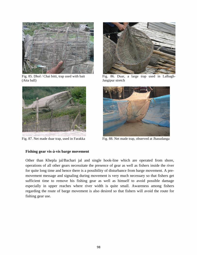
98
Fig. 85. Dhol / Chai bitti, trap used with bait (Atta ball)
Fig. 86. Duar, a large trap used in Lalbagh-Jangipur stretch
Fig. 87. Net made duar trap, used in Farakka Fig. 88. Net made trap, observed at Jhasudanga
Fishing gear vis-à-vis barge movement Other than Khepla jal/Bachari jal and single hook-line which are operated from shore, operations of all other gears necessitate the presence of gear as well as fishers inside the river for quite long time and hence there is a possibility of disturbance from barge movement. A pre-movement message and signaling during movement is very much necessary so that fishers get sufficient time to remove his fishing gear as well as himself to avoid possible damage especially in upper reaches where river width is quite small. Awareness among fishers regarding the route of barge movement is also desired so that fishers will avoid the route for fishing gear use.

99
6.11 Bank Erosion, Flow and Associated Changes
When vessels move through the water body, different waves are generated. As the propagation of deep-water divergent waves is unaffected by water depth, the waves will propagate at speeds dependent on their individual wavelengths (Newman, 1977). The longer period waves will travel faster and the shorter period waves will travel slower. If a wave trace is taken at different distances away from the sailing line, the trace will show the wave packet to be lengthening further from the sailing line as the individual waves spread out. It is essential to measure the actual amount of bank erosion in order to determine precisely the effect due to the passage of single barge.
Erosion is a concern for reasons relating to aquatic habitat, water quality, and loss of property as well as disruption of natural sedimentation processes in rivers and lakes. Waterways of all kinds are beneficial to society in many different ways. Not only do they provide recreational opportunities, but they also effectively discharge floodwater, dilute effluents, support the fishing industry, carry freight, provide transportation, and are often the main source of drinking water for nearby communities. Waterways are also very important ecologically, as they support a very rich and diverse community of plants and animals (Bonham, 1983). It is important for society to take responsibility to preserve our rivers, streams, lakes, and oceans for the ecological resources they provide. Bank erosion consists of two interactive physical processes: basal erosion and bank failure (Osman and Thorne, 1988; Darby and Thorne, 1996). Basal erosion refers to the fluvial entrainment of bank material by flow-induced forces that act on the bank surface: drag force, resistance force, and lift force. The rate of bank erosion traditionally has been calculated empirically from the geometry of channel bends, bank material, and flow intensity (Hooke, 1995). Process based bend migration models (Ikeda et al., 1981; Johannesson, 1985; Odgaard, 1989a,b; Crosato, 1990; Sun et al.,2001a,b) were successfully applied for long-term trends in meandering evolution. Most bank erosion occurs during the few largest floods each year. In these events, banks are exposed to the greatest height of floodwater, and the erosive stresses resulting from current velocities and water depth are also at their maximum. As water levels recede, the transported material is deposited in areas of low velocity (principally the insides of bends, thus balancing the erosion taking place immediately opposite). Deposition also occurs whenever the floodplain is inundated, as velocities outside the channel are always relatively low. Wave energy generated due to the passage of barges is a major concern as it increases the potential for erosion of river banks, shorelines, and levees. A significant effort has been made by many scientists to better understand the process of barge wake-induced erosion in many parts of the world such as the California Delta (Bauer et al., 2002), Marlborough Sounds in New Zealand (Parnell, 2007), the Kenai River in Alaska (Dorava & Moore, 1997) and the Illinois and Mississippi River systems (Bhowmik, 1981). This is an extraordinarily challenging technical task (Bauer et al., 2002), and the overall impact of a barge passage depends on a large number of factors including the distribution of wave heights in the wake packet, the wave period, and the overall duration of the wave event including waves that are reflected from the bank only to interact with late-arriving waves from the barge. Damage caused by barge wakes cannot be

100
solely blamed on large vessels because barge size does not determine the number of waves created by a barge. Even small barges can generate the same number of waves as a large barge. In this context, the appropriate question to be addressed is not whether barge wakes cause erosion, because they most certainly do to some extent. Rather in this juncture the more significant question deals with the present study is to understand the degree to which barge-wake induced erosion might be accelerating or substantively modifying the natural tendency for rivers to erode and rebuild their banks as part of the meandering process.
6.11.1 Study area
Natural Dynamics of Rivers Humans have always been interested in the dynamics of free-flowing water, and at the same time, are constantly attempting to restrain the natural flow of rivers. Since the Bhagirathi-Hooghly river channel (Fig. 89) is almost flowing in a plain terrain, natural meandering occurs in many places. They have complex feedback loops that yield complex adjustments. This channel is at a constant state of adjustment between erosion and deposition along its length. Erosion typically occurs on the outside of a meander bend where the current is the largest, while deposition is found to occur on the inside of a meander-bend. As erosion occurs, the eroded material typically contributes to deposition downstream of the river thereby sustaining a continuous series of interconnections along the longitudinal profile of the river system. It is observed that meandering and channel shifting are important processes in this fluvial ecosystem.

101
Fig. 89. Location map of the study area
It is important to appreciate that even if barge traffic were to be eliminated completely from a river system, erosion by natural factors would still proceed (Maynord et al., 2008). Thus, it is critical to understand the natural dynamics of rivers as the natural back-drop against which the impact of barge traffic can be assessed. Changes in channel position are inevitable and it has been witnessed by the remote sensing imageries, along with recurring flooding events. A schematic diagram of the study conducted in six different locations along the meander is shown in Fig.90. The study pertains to one barge (72m x 14m x 4.5m) movement along the course of the river, further it was conducted in a low tide and during non-flooding period.
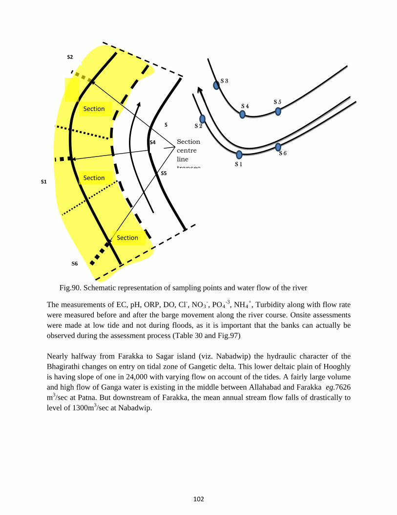
102
Section centre line transec
Section
Section
Section
S
S4
S5 S1
S2
S6
S 1
S 3
S 2
S 5 S 4
S 6
Fig.90. Schematic representation of sampling points and water flow of the river
The measurements of EC, pH, ORP, DO, Cl-, NO3-, PO4
-3, NH4+, Turbidity along with flow rate
were measured before and after the barge movement along the river course. Onsite assessments were made at low tide and not during floods, as it is important that the banks can actually be observed during the assessment process (Table 30 and Fig.97) Nearly halfway from Farakka to Sagar island (viz. Nabadwip) the hydraulic character of the Bhagirathi changes on entry on tidal zone of Gangetic delta. This lower deltaic plain of Hooghly is having slope of one in 24,000 with varying flow on account of the tides. A fairly large volume and high flow of Ganga water is existing in the middle between Allahabad and Farakka eg.7626 m3/sec at Patna. But downstream of Farakka, the mean annual stream flow falls of drastically to level of 1300m3/sec at Nabadwip.
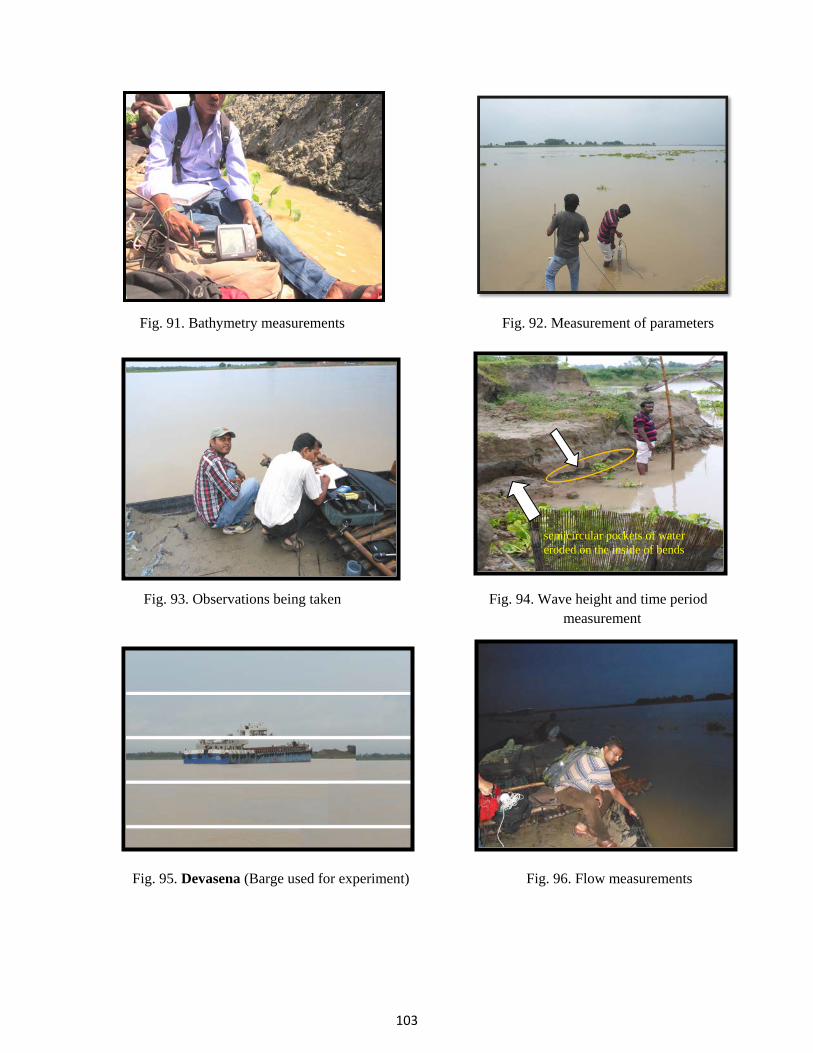
103
semicircular pockets of water eroded on the inside of bends
Fig. 91. Bathymetry measurements Fig. 92. Measurement of parameters
Fig. 93. Observations being taken Fig. 94. Wave height and time period measurement
Fig. 95. Devasena (Barge used for experiment) Fig. 96. Flow measurements

104
Table 30. Parameters observed at Srirampur before and after the barge movement
Station (S1) 23.19°.40.1,88°.22°.49.0
Before After
NH4 (mg/l) 0.13 0.11 ORP (mV) 322 350 PO4 (mg/l) 0.0784 0.0792 Conductivity (µS/cm) 175.2 173.9 Cl- (mg/l) 12.81 10.09 NO3 (mg/l) 0.600 0.509 DO (mg/l) 6.13 6.20 Turbidity (NTU) 274, 264 299.8 Flow (m/sec) 0.28, 0.30 0.52 -0.71 STATION (S2) AFTER BEFORE NH4 (mg/l) 0.12 0.12 0.12 ORP (mV) 364 344 345 PO4 (mg/l) 0.0788 0.0790 0.0789 Conductivity (µS/cm) 175.0 173 173 Cl- (mg/l) 10.92 8.05 7.69 NO3 (mg/l) 0.595 0.759 0.723 DO (mg/l) 6.16 6.20 6.17 Turbidity (NTU) 242.1 292 Flow (m/sec) 0.07 0.14 0.16 0.10 0.05 0.16 0.08 0.12 0.18 0.11 Middle Channel (23°19’31”.0,88°22’35”.5) Station (S3) Before After Temp (oC) 29.90 29.91 NH4 (mg/l) 0.12 0.11 ORP (mV) 371 366 pH 7.91 7.92 Conductivity (µS/cm) 174.6 173.9 Cl (mg/l) 12.56 12.54 NO3 (mg/l) 0.545 0.531 DO (mg/l) 6.25 6.29 Turbidity(NTU) 252.2 250.5 Flow(m/sec) 0.30/0.36 0.32/0.30 Depth(ft) 2.1 1.5

105
Station (S5) Before After Temp (oC) 29.78 27.58 NH4 (mg/l) 0.20 0.10 ORP (mV) 385 370 pH 7.95 8.06 Conductivity (µS/cm) 172.6 172.6 Cl (mg/l) 9.30 9.19 NO3 (mg/l) 0.843 0.736 DO (mg/l) 6.37 6.42 Turbidity (NTU) 353 366, 367 Flow (m/sec) 0.59 0.64 0.55 0.57 0.58 0.62 Station (S6) 23°19’40”.1,88°22’48”.0
Before After
NH4 (mg/l) 0.12 0.12 ORP (mV) 362 362 pH 7.89 7.89 Conductivity (µS/cm) 172.8 172.8 Cl (mg/l) 9.66 8.67 NO3 (mg/l) 0.610 0.598 DO (mg/l) 6.16 6.17 Turbidity (NTU) 174.0 192,193.4 Flow (m/sec) 0.67 0.7,0.71

106
0.1
1
10
100
1000 Before AfterStation - 1
050
100150200250300350400
Station - 2
0.1
1
10
100
1000
Station - 3
0.1
1
10
100
1000
STATION 5Station - 5
0.1
1
10
100
1000
Station - 6
Fig.97: Variation of physical and chemical parameters before and after the barge movement

107
Fig. 98. Year wise variation in bank erosion at Bhagirathi-Hooghly river (mm)
The normal erosion trend observed by the previous workers reveal the fact that there has been more erosion during the period from 1975-76 (Fig. 98) due to heavy floods in the region which has increased the velocity of the river.
6.11.2 Data used
Based on satellite image quality and availability the primary data of LANDSAT satellite for two different periods in ten years interval were considered for analysis (Table 31). Table 31. List of satellite imagery
0
5
10
15
20
25
30
35
1973 1978 1983 1988 1993
Eros
ion
in m
m
Satellite Path/Row Year
LANDSAT-7 139043, 138045,138044 2000
LISS – IV 107-57a,55b,54d,54c,54a,55d;
108-55c,56 a,c,
2014

108
6.11.3 Data processing and analysis
The river channel and associate land cover mapping were done in few steps (Fig. 99). All the
scene Landsat images were not acquired as rectified image. Topographic maps, LANDSAT-7
and LISS-IV. All images were resampled with the nearest neighbour method to a common
resolution of 30 m. Resample was chosen to a common resolution so that river of interest would
be either equal to or larger than the pixel size.
Fig. 99. Flow diagram of the whole study

109
Fig. 100. LANDSAT image extracted for 2 km from the river
After that Landsat images were processed in ERRADAS. Compared with pixel-based methods, this approach shows better classification results with higher accuracy as it uses both spectral and spatial information (Civco et al., 2002; Yoon et al., 2004; Harken and Sugumaran 2005; Gao et al., 2007). The most important issues in the context of an object-oriented classification is the

110
accurate segmentation of the input images. In the present analysis, the ‘‘multiresolution’’ algorithm was used; this algorithm locally minimized the average heterogeneity of image objects for a given resolution. For each segment, information on average NDVI, Land and Water Mask slopes were derived (Fig. 100). This information was used to develop suitable classification algorithms for individual classes. Image objects were linked to class objects and each classification link stored the membership value of the image object to the linked class. With each polygon assigned to a specific class, land cover map including river channel was generated for Srirampur area of the river after the classified data was exported to shape file format for further processing, such as the elimination of areas smaller than the defined minimum mapping units. Centre line of river was generated from river channel. Within 2 kilometers of river centre line, settlement/landmark/building were identified from topographic maps using ArcGIS. Threat on settlements were analysed based on number of time river flew through particular settlement location. The comparison of the river channel location was carried out for a period from 2000 to 2014 for the riverbanks.
6.11.4 Movement of riverbank at pair positions
All classified images are transferred to GIS layers using ArcGIS 9.3. Land covers in 2000 are taken as initial state. Evaluation is performed based on this initial land covers. The pair positions at the east and west banks of the Srirampur area of the river for each site are identified on the GIS layers in 2000. A standard measurement tool of ArcGIS is applied to measure the distance between the initial location of those pair positions at the riverbank in 2000 and 2014 and the nearest riverbank in the previous particular year. Thus, it explains the movement of riverbanks at those selected locations based on the initial river channel in 2014. Movements of the riverbank at a certain location indicate erosion. This can be called a back casting trend analysis, by which it can be analyzed what was the land cover of a certain position, which is now at the riverbank. If pair position is located at all other land covers except water/river in previous particular year that is at riverbank in 2000, then the distance between this point position and nearest riverbank indicates vulnerability. This vulnerability is positively proportionate to this distance. It indicates erosion. However, the location of pair point at water/river in a same manner indicates deposition, which is considered more suitable for bridge construction.

111
6.11.5 Results and discussion
At Srirampur an imbalanced hydro-morphological conditions exist due to wave action, tidal effect. The rate of erosion and its location have, however, has changed during the time period.
Results of interpretation and extracted layers from satellite images were transformed into GIS layers in vector format. Change of river segments was detected by superimposing data layers
Fig. 101. The spatial location of regions with higher slope along the bank of the river
112
together by the order of raster-vector or vector-vector. Erosion and accretion of the river were digitized considering (2000 and 2014) with vector shape file. The estimation of the area was made with the aid of GIS. Data of different periods (from 2000-2014) were considered for erosion and deposition area calculation. The bank line change map was prepared and superimposed layer by layer as a vector file with backdrop base imagery. All the layers superimposed one by one maintaining sequential order, there after change detection was performed, demarcated and calculated the erosional and depositional regions of the study area from 2000 and 2014 and final layout were developed for visual interpretation and presentation which are showing in Fig. 101. LISS – IV recent available imagery was considered in 2014 for the base and standard bank line. From the calculated results of different erosion and deposition, different types of erosion and deposition zone were identified.
The slope map was prepared from DEM of 30 m resolution for 2 km along the river course. Nine different categories were represented as shown in the Fig. 101, representing from <1.6 o to >45o. The map indicates that there are three major regions vulnerable to erosion, with slope >45o. The major portion of this greater slope is located in the northern part of the river just south of the Farakka and the second zone is in the central part of the river and the third one is south of Srirampur. Further it is interesting to note that the slope is more prominent where the sinuosity of the river is predominant, represented by meanders.
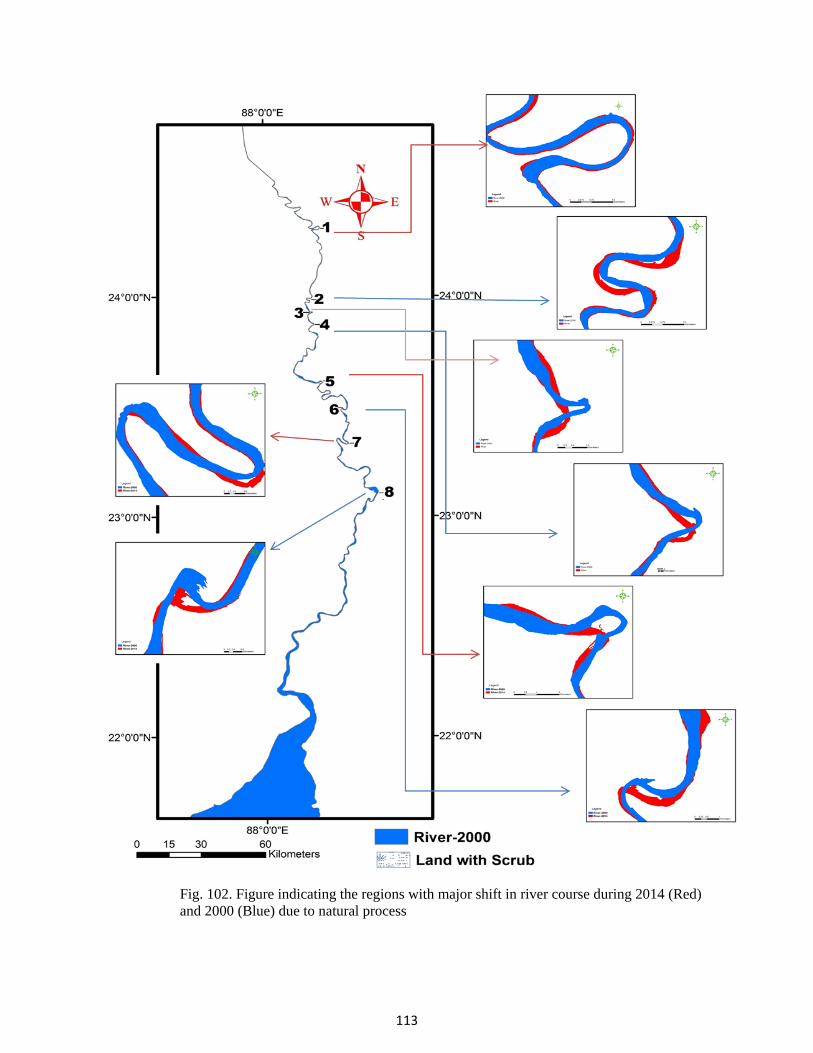
113
Fig. 102. Figure indicating the regions with major shift in river course during 2014 (Red) and 2000 (Blue) due to natural process

114
Analysis of a series of images, exposed the dynamic nature of the river bank and, including channel migration, movement. The changes of river channel from 2000 were very high and unstable. The river channel location changes are presented in Fig. 102. The total area occupied by river during 2014 is 2303 sq km and the area inside the river indicating land with scrub is about 344 sq km and the area occupied by the river during 2000 is 1926.53 sq km (Fig. 102). The river shift shows that it has resulted in changes along the settlement/ landmark/ building, in particular land settlement due to the river channel changes had flattened. There is evidence of severe bank erosion and rapid rates of bank line retreat along the Surjapur in the river channel. This happens to a channel due to morphological adjustments to accommodate the range of flows and sediment loads from upstream (Khan et al., 2003). The water level changes and fluctuation in the dry season would not cause frequent riverbank erosion compared to the same changes and fluctuations in the wet season.
The study demonstrates efficient way to determine river channel and understanding river erosion and siltation and how it has trended on settlement alongside the Bhagirathi-Hooghly River using remote sensing and GIS from medium resolution Landsat images and topographic maps. This type of study is obliging for further planning of river and river adjacent to settlement management in an effective manner as it could be incorporated the long time changes of the river morphology. GIS analysis result of 2000 and 2014 has shown significant changes in the river course. Erosion and siltation were regular processes and in large area of the river it has occurred.
Data analysis from 2000 - 2014 shows that the increase in river course is about 376 sq km and area near Surjapur and Srirampur is more vulnerable to erosion. The river course shows an overall migration of the meanders along the flow direction. Further increase of channel width is also noted during 2014, which is mainly due to the increase in volume and velocity of the river. The tidal effects, combined flow of river and regular channel shifting are mainly responsible for erosion in that area. Higher rate of deposition may help to form submerged land or char land which may divert the water flow to the mainland resulting severe erosion. Past protections or embankments which were given to reduce erosion, failed in most of the areas and also increased erosion rate in the unprotected areas.
River bank erosion is basically here due to slumping down or carrying away the bank of the river by itself and it affects the changes in river channel courses in alluvial plains (Fujita et al., 2000). Erosion has been defined as the mechanism of detachment of sediment particles and other materials from the land surface or erosion is the combined processes of detachment and transportation of soil materials by the action of flow, waves, tidal fluctuations and other hydrological factors governing the flow condition of a channel (Ahmed, 1989). One of the most serious problems in Bhagirathi river channel is erosion of river. Analysis of imageries, between 2000 and 2014, exposed the dynamic nature of the river bank and, including channel migration, movement. The changes of river channel from 2000 to 2014 were high and unstable. The river channel location changes during the period 2000 to 2014 are presented in Fig. 102. The average bank erosion was 376 km2. There is evidence of severe bank erosion and rapid rates of bank line retreat along the Bhagirathi River. This happens to a channel due to morphological adjustments
115
to accommodate the range of flows and sediment loads from upstream. (Khan et al., 2003). In 2000 to 2014 water area in the river has a lot of dissimilarity. This variation could be because of seasonal deviation of satellite image or other reason. The water level changes and fluctuation in the dry season would not cause frequent riverbank erosion compared to the same changes and fluctuations in the wet season (Lu, 2006). The channel erosion in 2000-2014 was relatively increased. Migration of river channels in regions 1-8 (Fig. 102) doesn’t indicate only erosion of riverbank. It means either erosion or deposition. However, most of the cases, in this study, erosion of riverbank are observed. Further, the study has led to the conclusion that there is an increase in the width of the river channel in straight courses and shift in river course along the meanders. This shift is mainly due to the variation in the erosional and depositional capacity of the river from 2000- 2014.
6.11.5.1 Turbidity
Turbidity can be a result of a number of factors, some natural and some human induced. The extent of boat/propeller induced turbidity appears to be influenced by a number of variables relating both to the boat and engine and to the characteristics of the water body. These variables include the depth of the water, the speed and power characteristics of the craft, the characteristics of the propeller/water jet, the distance the boat travels from the shore, the duration and extent of boating activity and the characteristics of the water body sediments. The depth of the water - boats have a greater opportunity to create turbidity when travelling in shallower water as the downward pressure of water created by the craft reaches the sediment with greater energy. The effect of engine power - a more powerful engine has the capacity to create more turbidity than a smaller one. It is thought, however, that a planing boat may create less turbidity as the craft is effectively lifted out of the water and, therefore, causes less underwater disturbance. In general, a horizontally angled propeller will have a lesser effect on the bottom sediments as its energy will be more dissipated when reaching the water body bed than that of a propeller which is more vertical in orientation.

116
Table 32. Turbidity measurements for before and after the barge movements in river
Turbidity(‘B’ before the barge movement – ‘A’ after the barge movement)
Average Difference(A-B) Percentage
S1 B 274 264 269 30.8
5.4 A 299.8 299.8 S2 B 242.1 242.1 54.4
10.1 A 292 301 296.5 S3 B 252.2 252.2
-2.2 -0.4 A 250 250 S4 B 250.5 250.5 -0.5
-0.1 A 250 250
S5 B 35.3 35.3 1.35
1.87 A 36.6 36.7 36.65 S6 B 174 174 18.7
5.09 A 192 193.4 192.7
The turbidity has been measured as an indicator of sediment suspension by waves and the environmental impact of boating activity (Downing et al., 1981; Garrard and Hey, 1987). Turbidity monitoring indicates that it causes bank erosion as observed by Bradbury(2005). Turbidity measurements along the meander of a river were made at S1, S2, S3, S4, S5, S6 (Fig. 97). Samples have been measured in both sides of the river. Turbidity and flow rate has been measured before and after the barge movement. In the locations S1, S2, S5 and S6 turbidity increased after the barge movement (Table 32). In S3 and S4 turbidity was recorded to decrease. S3, S4 and S6 are present in the shallow depth whereas another side of the river i.e. locations S1, S2 and S6 have a deeper bathymetry conditions where the meander appears. Erosion occurs on the outside of the bend, and a helical flow of water then deposits eroded material from this bank on the inside bank of the bend. Resuspension and stirring of bottom sediments has been found to begin occurring depths shallower than about 3 meters. However, at depths of approximately 2.2 meters or less resuspension occurs much more significantly (Beachler and Hill, 2003). Waves generated from barge traffic have the ability to suspend sediment for long periods of time even after the wave group has passed and be transported downstream (Houser, 2011).
As flow depths and velocities increase, the force of the water flowing against the stream bank removes soil particles from the banks, and in many cases erosion causes banks to slump and fall into the flowing water. So the barge moves near this side and at the same time turbidity increases which results in the bank erosion. It is interesting to note that S3 & S4 locations which are situated in shallow depth, turbidity did not show any variation after the barge movement. The higher percentage of turbidity is noted in S2 location. The study also reveals the fact that there is an increase of 5-10% of turbidity in deeper regions and nil – 2% of increase of turbidity in the

117
shallow regions. It is a fact that in a meander the sailing line is close to one side of the bank with deeper bathymetry.
Its total energy from the series of waves in the wake of one boat does not decline significantly while the wave travels up to 100 feet across water. Distances over 400 feet were needed to reduce wave energy. Natural river currents generally erode the outside of curves in rivers and deposit sediment on the inside of bends. There found unnatural semicircular pockets of water eroded on the inside of bends, up to a foot in diameter. They observed these being eroded by successive boat wakes, similar observation of 14 feet diameter was noted in Gordon River (Dorava and Moore, 1997).The study seems to indicate that boat wakes do indeed contribute to the erosion problem on the River, but the extent of their contribution remains difficult to quantify with any degree of certainty. Boat wakes may still play an important role by eroding the material that has been deposited on the gently sloping apron that is adjacent to the cut bank, including large slump blocks that recently calved off the bank into the water (Larissa Laderoute & Bernard Bauer, 2013).
Table 33. Flow measurements for before and after the barge movements in river
Flow (m/sec) Average Difference Percentage S1 Before 0.28 0.3 0.10 0.11
35.91 After 0.52 0.71 0.21 S2 Before 0.07 0.14 0.05 0.16 0.18 0.11 0.12 -0.04
-21.37 After 0.16 0.1 0.08 0.12 0.08 S3 Before 0.36 0.3 0.11 0.01
5.71 After 0.38 0.36 0.12 S4 Before 0.32 0.301 0.10 0.002
0.72 After 0.32 0.31 0.11 S5 Before 0.59 0.55 0.58 0.29 0.02
3.10 After 0.64 0.57 0.62 0.31 S6 Before 0.67 0.11 0.12
35.58 After 0.7 0.71 0.24
Flow rate increases in the channel after the barge movement (Table 33) in all locations except in the location S2. This is mainly due to the percentage increase of turbulance which decreases the flow rate in S2 and results in bank erosion. Erosion occurs when boat induced current velocity and turbulence is more powerful than the weight of the soil particles and their cohesive strength. Therefore it’s inferred that cohesive soils (e.g. clay soils) are more resistant to erosion than non-cohesive soils (e.g., sandy soils). The field observation indicated that pockets of erosion are mainly due to nature of soil, vegetation cover, velocity of water and the direction of flow.

118
050
100150200250300350
Ave
rage
Mon
tly ra
infa
ll fo
r 22
year
s (m
m)
Berhampur
Mass slumping in vertical face of the bank
semicircular pockets of water eroded on the inside of bends
Differential strands levels of erosion due to various flood Erosion due to wave
action enhanced by silty materisla slong the bank
Fig. 103. A view of the vertical face of the bank eroded by mass slumping due to undercut action
6.11.5.2 The rain fall observations
The monthly average record of the meteorological station near Berhampur reveals that higher rainfall is noted during June- September months of the year. This indirectly reflects on the flow of water along the river channel.
Fig. 104. Average monthly rainfall observation for 22 years

119
Hence it is inferred that the volume of water increases during the mentioned period. Moreover this is indirectly reflected on sediment load and velocity of river. The higher velocities during this period naturally induce erosion along the river banks. The movement of barge along the river channel during this period enhances the erosional capacity of the river more than during the normal periods (Fig.104). During these periods barges have to move on an optimal speed than the normal speed on knots. This rainfall data is further correlated with the stream flow in the river which also reflects the fact that the velocity is higher during monsoon (Table 34).
Table 34. Monthly stream flow (m3/sec) in Bhagirathi/Hooghly at Nabadwip (Purbasthali) between 1975-81
Month 90 percentile flow 50 percentile flow 10 percentile flow Means January 922 1026 1188 1048 February 938 1021 1163 957 March 393 875 1063 838 April 350 884 1081 829 May 596 1105 1159 1013 June 1123 1266 1402 1263 July 1392 1824 2237 1817 August 1663 1380 2235 2000 September 1380 2120 2600 1995 October 1928 1519 2407 1734 November 927 1055 1132 1041 December 1106 1222 1293 1203
6.11.5.3 Basic wave mechanics
When a barge is loaded the return current and the supply flow are the dominant phenomena for banks. The direction of the return current and the supply flow are parallel to the channel flow. The return current is in the opposite direction to the ship's sailing direction, while the supply flow is in the same direction. The aft boundary of the water level depression caused by the return current is called the transversal stern wave and here the change in flow direction between the return flow and the supply flow occurs. Normally the propeller race has no direct impact on bank stability.
The size of the secondary waves depends on ship speed and thus are only important in relation to bank erosion, when ships sail relatively fast, which is not the case with loaded push-tow units. As a barge travels through the water, it generates a series of waves. The height and period of these waves vary depending on boat speed and type. Once fully formed, the groups of waves are termed a ‘wave train’. In deep water the height of the waves within the wave train will attenuate with distance, though the period will remain relatively unchanged. The key descriptors of these waves are schematically displayed in Fig. 105.

120
River bank erosion is driven by the energy exerted by the flow on the banks. In most rivers, the source of energy is the downstream flow of water, which creates near-bank currents that apply shear stresses on the bank materials. When the bank materials (gravel, sand, silt, clay) are able to resist this shear stress, then there is no bank erosion. However, when the shear stress exceeds the threshold for entrainment of the bank materials, erosion occurs.
Fig. 105. Water movement around a ship from channel flow without groynes
The same situation applies to waves that impinge on the shoreline regardless of whether their source is from barge passages, wind forcing, or nearby landslides. The amount of energy contained in single wave is proportional to wave height (trough to crest distance) and to wave period (time needed for a full wave cycle to travel by a single location (Fig.105). As these two factors increase, the wave energy increases non-linearly according to the following relation:
E = 1/8 ρgH2L ----------------------------- 1 where E is the total energy contained in a wave of wavelength, L, and wave height, H. Water density, ρ, and gravitational attraction, g, also are essential parameters in the relationship. Note that for simple surface gravity waves in 'deep' water, L (given in metres) is proportional to the wave period, T (given in seconds), such that L = 1.56 T2.
A
B
C
E
F
G
E
F
A. Front wave B. Water level depression C. Transversal stern wave D. Return flow E. Supply flow
Ri
ver
Groyn

121
Fig.106. The maximum height of the wave and the time period as observed in the field after the movement of barge
The maximum height of the wave and the time period, in S1 is 5.2” and 0.76 sec; S2 is 4.2” and 0.7 sec and S6 is 8.1” and 0.814 sec., respectively. The energy calculated at these locations are 0.0193 J/m, 0.01067 J/m and 0.0533 J/m respectively at S1, S2 and S6 (Fig.106). In the other stations no significant variation of wave was noticed. However, in most instances the deep water wave solutions are not strictly applicable even though they provide a reasonable estimate of available wave energy given that there are several additional sources of uncertainty that enter into this complex problem. It has been reported that in deep water there is a definite relationship between the waterline length of the barge and the maximum wave height. It’s also observed in the field that the sailing line is along the deeper portion of the river channel. However, wave height alone is not an accurate indicator of potential for shoreline erosion. Energy, power, and energy per unit wave height are alternative methods of measuring the potential for erosion. The energy within a boat wake wave may cause damage to a shoreline by initiating sediment transport. Damage may be caused by the effect of a single wave or the cumulative effect of several wave trains from many boats. The preferred criterion for analyzing the relative effects of wave’s energy; a function of both wave height and wave period. Bank degradation is generally the result of a process that combines the erosive power of water and the effect of gravity. Wave energy calculations have been used to calculate both the maximum wave generated by a single boat pass, and the cumulative energy of multiple waves over a specific time period (Glamore 2008 ) E = ρg2H2T2 / 16π --------------------------2
0.81 sec
0.2
m S1
0.7 sec 0.
1 m
S2
0.76 sec
0.13
m
S6

122
Where, ρ is the water density, g is the gravitational constant, and π = 3.14 is a constant. The application of the above said formula to calculate wave energy per meter wave crest length also shows the similar results of Equation 1. 6.11.5.4 Froude number: The general wave pattern generated by a barge is largely independent of barge form, but it is affected by water depth and barge speed. The defining parameter is depth Froude number, a non-dimensional relationship between barge speed and water depth. Barges of different configurations travelling at the same depth Froude number will produce equivalent wave patterns. The following observations were made with a given Barge speed of 9 knots. The definition of depth Froude number, Frh, is: Frh = v/√gh -----------------------3 wherev is the velocity of the barge, g is the acceleration due to gravity, and h is the water depth, which is reflected by bathymetry. Depth Froude number has its greatest effect when the water depth is less than about one-quarter the barge waterline length; it has moderate influence at depths up to one-half the waterline length and has little influence at depths greater than the waterline length. The length Froude number is traditionally used to non-dimensionalize barge speed (Macfarlane, 2012). It is given by the following equation FrL = v/√gL, -----------------------4 Where v is the velocity of the barge, g is the acceleration due to gravity, and L is the barge water line length. The type of speed designated by the Froude numbers are as follows: Fd<1 and Fl <0.5, flow is subcritical (deep, slow speed); and Fd>1 and Fl>0.5, flow is supercritical (shallow, fast speed). It is believed that the amount of sediment transported and the direction of transport is highly dependent on the Froude number. Subcritical waves generate sediment transport in the landward direction at oscillatory frequencies, while supercritical waves generate sediment transport in the seaward direction at wave group frequencies (Houser, 2011). Most of the sampling sites at Srirampur and few of the Surjapur show subcritical speed and the waves pertain to have larger angle . The observation is based on the given speed of the barge as 9 knots. After waves are generated from the barge, the wave energy begins to dissipate away from the path of the wake. As the waves travel farther from the barge, they continue to change due to dispersion, friction, and gravity. These complex wave transformation processes are governed by a set of site-specific characteristics such as bathymetry and the angle at which the waves propagate away from the wake these are noticed along the meanders. Waves generated at supercritical speeds tend to have a small angle of divergence (4-10°), while waves at subcritical speeds propagate at a large angle (20-30°) (Houser, 2011). Most of the waves reach the shoreline, they will change shape, size, and direction as a result of refraction, shoaling, and breaking. When the waves come in contact with the bed and banks, sediment may become detached and transported due to the wave energy. Transport of the sediment in the direction of the wave occurs due to the orbital motion of waves (Kirkegaard, 1998). The orbital motion is the motion beneath the wave.
The motion is larger and oblong near the surface and gradually becomes smaller at depth, which implies that the forces that a wave is able to exert on the bottom are attenuated (i.e., reduced)

123
deeper in the water column. Most barges -wake waves generated by barge traffic are of short period and short wavelength, and these types of waves don't have any impact in deep water. But as they migrate toward the bank and interact with the sloping bottom, they can be quite erosive.
Fig.107: Critical speed zones
The water depth limits (Fig.107) the speed at which a wave can travel in shallow water, such that the maximum speed will be reached when the depth Froude number equals one. Almost all the Kohrnash observation station and 75% of Surjapur station fall in this category. At a vessel speed below a depth Froude number of one, the speed is said to be sub-critical, as that of Srirampur. A depth Froude number of one is termed the critical speed and speeds around the critical speed are sometimes referred to as trans-critical speeds (approximately 0.8 ≤ Frh ≤ 1.2). The position of the upper and lower bounds of the trans-critical range can vary according to vessel and waterway conditions. Speeds above a depth Froude number of one are said to be super-critical. These zones are shown graphically in Fig.108. When viewed from above (Fig.108), the super-critical divergent wave pattern looks different to the sub-critical wave pattern. The super-critical pattern consists of long-crested waves, whereas the sub-critical pattern consists of a series of shorter-crested waves. 6.11.5.5 Sub-critical speeds
In deep water, defined as being a depth such that the depth Froude number is less than 1 (more importantly, when the depth Froude number is less than about 0.7), all barges produce a wave pattern termed the Kelvin wave pattern, named after Lord Kelvin, an early pioneer of vessel wave theory, Kelvin (1887).

124
A typical Kelvin wave pattern is presented in Fig.108. It is characterized by two wave types - transverse and divergent waves. This is characterized in 40% of observation sites in Surjapur, 80% of the observation sites at Srirampur. Transverse Waves These waves are commonly referred to as stern waves and propagate parallel to the barge's sailing line. The height of these waves is largely a function of vessel displacement-length ratio, with a heavy, short barge producing higher waves. The period of the transverse waves is a function of barge speed, as they effectively travel along with the barge. Divergent Waves Commonly referred to as bow waves, the divergent waves propagate obliquely to the barge's sailing line at an angle of approximately 55 degrees. This wave formation, referred to as the Kelvin wedge, subtends an angle of slightly less than 20 degrees to the sailing line, which is constant for all barge forms. Many vessels also create stern divergent waves, though this additional wave train usually melds into the bow divergent system at some point aft of the vessel. Divergent waves are generally steep and close together near the barge - carrying as much energy as possible for their wavelength. The following phenomenon was observed in the Srirampur meander observation during the time of barge movement experiment. The point of intersection of the transverse and divergent wave trains is termed the cusp and represents a localised wave height peak. At successive cusps, the divergent waves decay in height slower than the transverse waves, such that a vessel wake measured far from the sailing line will feature divergent waves more prominently. The oblique propagation angle of the divergent system compared with the transverse system means that the divergent system is usually of greater interest when assessing erosion, as these waves propagate towards the steep banks. The studies have also proved exceptions to this; If a barge is producing a significant transverse wave system, such as a heavy vessel, changes course, the transverse waves created prior to the
Fig 108.Sub – critical speed representation
• Fd<1 • Short – crested divergent
waves • Transverse waves present
Divergent waves Kelvin wedge cusp angle 19o28”to sailing line
Transverse waves
cusp

125
course change will continue to propagate along the original course and may eventually reach the shore. This is commonly noted when slow speed displacement vessels traverse a narrow river at cruising speed. The river traps the transverse waves and does not allow them to diffract (spread their energy by growing sideways in crest length), greatly reducing their height decay. These waves may be evident for several minutes after the vessel has passed. The total energy of the wave train is equal to the sum of the energy of each individual wave, which was observed to persist for 2 minutes at S2, 2minutes 21sec at S1 and 1minute 48sec at S6. 6.11.5.6 Critical speed
When the depth Froude number approaches unity, which can occur when either the water depth shoals or when the barge's speed changes relative to the water depth, the wave pattern changes (Sorensen 1973a). As the waves reach their depth-limited speed, the divergent waves increase their angle to the sailing line, propagating more in line with the stern transverse waves (Fig.109). At the critical speed, when the depth Froude number equals one, a vessel will experience a peak in resistance. The relative magnitude of the resistance peak is dependent on the ratio of the water depth to vessel waterline length, with very shallow water for a given waterline length producing the most pronounced increase in resistance. Few observation stations at Surjapur and one at Kohrnash represent this category The observation shows that wave pattern generated consist of only one long-period wave, termed a wave of translation, propagating parallel to the sailing line. This single wave travels with the barge and so does not radiate from it. It does, however, grow in crest length - the barge pumps energy into this wave that is initially accommodated as a height increase, but once height stabilises the wave grows in crest length. The speed of this crest length growth equals the barge speed. If banks bound the water at the sides, limiting energy growth in the single wave, a train of several waves, termed solitons, may then form ahead of the barge if the conditions are conducive to their formation. These waves of translation are particularly damaging and are to be avoided by maintaining the barge speed. Not only are they difficult to see, having a long period but low height, they are hard to maintain under real-life conditions. It is common for barges operating in
Fig. 109. Representation of Critical speed • Fd = 1 • One or more waves perpendicular to the sailing line • Crest length grows (sideways ) a at a rate equal to
the vessel speed

126
shallow water to operate at speeds that may be depth-critical at times and the Master needs to be aware of this and avoid the critical speed or pass through it quickly. The damaging effects are a non-linear function of barge displacement. 6.11.5.7 Super-critical speeds At speeds above the depth-critical speed, a barge's wave pattern changes again (Fig.110), most of the observation locations of Kohrnash and 50% of Surjapur shows that the 9 Knots will be super critical speed and it has to be further reduced.
The observation shows that transverse waves, which travel at the speed of the barge, are no longer able to travel at the barge speed due to the limiting relationship between maximum wave speed and water depth. As the barge accelerates from a sub-critical to a super-critical speed, the transverse waves fall behind the barge and disappear altogether. The lack of a transverse wave train reduces barge wave making resistance, which explains why many barges go faster in very shallow water. The divergent waves also re-appear in their more usual form, but propagate at an angle to the sailing line that is dependent on the barge's speed, such that the velocity vector parallel to the barge's sailing line is not more than the critical speed. The higher the super-critical barge speed, the less acute the propagation angle becomes. For very high-speed craft operating in relatively shallow water, it often appears that the divergent waves propagate almost perpendicular to the sailing line.
The divergent waves propagate from deep to shallow water, or are created in shallow water to begin with, the waves begin to feel the bottom and become depth-influenced. When the speed of each wave is depth-critical, that is, the depth Froude number for each wave equals unity, the maximum speed of propagation becomes limited to the depth-critical speed. A wave packet will then stop dispersing and the waves will travel at the same depth-limited speed. Waves Non-dispersive waves are also noted along the shallow region (Shallow water waves). With the divergent wave packet being comprised of many waves with different wavelengths, the waves with long wavelengths will become speed limited and therefore non-dispersive before those slower waves with shorter wavelengths. Though there may be some leakage of wave energy in a non-dispersive packet, but this is only evident over several barge lengths of shallow water wave propagation.
Fig. 110. Representation of Super – critical speed
• Fd>1 • Transverse waves die away • Long –crested divergent
waves • Long-period leading waves

127
Dispersion creates difficulties when assessing wave traces obtained. Where a trace taken close to a vessel as that of observation at S6 (within, say, half a barge length), the trace may appear to consist of only a few waves, when in fact these waves represent many more waves of differing wavelength superimposed. It takes approximately 2-3 barge lengths for waves to disperse sufficiently such that the period of individual waves can be measured with certainty, as observed at S2. 6.11.5.8 Displacement speed
All barges have a displacement speed range where the length of the transverse waves generated is less than the waterline length. If the speed of the barge is maintained 9 knots then the transverse wavelength is lesser FL is less than 0.399 (Fig.107). The upper limit of this speed range is when the length Froude number when the speed of the barge reaches 20.619 knots, Fr, equals 0.399, which reduces to: v = 2.43√L. the calculations are arrived with a barge water line length of 72m. This maximum displacement speed, or hull speed, represents the condition where the longest wave generated equals the waterline length of the vessel. To travel faster than this, the vessel must begin to climb its own bow wave (the common analogy). Wave making resistance in the displacement region is proportional to v6, so small changes in speed cause large changes in resistance and wash. In the displacement speed region, wave periods are modest and wave making energy transforms into wash height, creating steep waves. In general, operating at speeds up to 75% of the maximum displacement speed (or about 1.82√L knots) will produce modest wash height and period. The present speed of the barge derives a relation of 1.061√L knots. 6.11.5.9 Semi-displacement speed
As a barge powers through the displacement speed limit, its running trim increases as the transverse waves move aft of the transom. Barge wave making resistance is high, peaking at a length Froude number of approximately 0.5. Wave wake height increases to its maximum and divergent wave periods increase steadily. A particular operating condition to be avoided is at a length Froude number of 0.5 and depth Froude number of 1.0, when maximum specific wave making resistance and depth effects coincide. This condition occurs when: h= 0.25L and v = 3.04√L Semi-displacement speeds, often referred to as hump speeds in planing craft terms (when the vessel appears to climb over the hump before planing) create damaging wash. When the bathymetry is at 18m and the barge speed is at 25.79 knots (Fig.107). 6.11.5.10 High speed As the length Froude number increases above 0.5, specific wave making resistance slowly reduces. The maximum wave height reduces and maximum wave period levels to a relatively

128
constant value. Wetted surface area, the basis of frictional hull drag, becomes the principal drag component, hence the drop in total wave wake energy with increasing speed.
Fig.111. Vessel speed regimes
When there is a high-speed >25.79 knots barge wake its noted that there is semi-displacement speed, where waves are high and steep (Fig.111). This may appear to be the case, but the high-speed condition produces the longest wave periods, which may have as much or greater effect on shorelines and shoreline structures as wave height. It is important to remember that wave height attenuates with distance from the sailing line but period remains constant.
6.11.5.11 Other factors There are other factors that contribute to erosion that must also be considered. Natural forces include the river currents (especially during floods), wind generated waves (especially during high-wind events and across long or wide fetches of water), and geotechnical processes that lead to bank slumping events. However, bank characteristics that affect stability such as vegetation, the height and slope of the banks, stratification, gain texture, and grain size will also determine the ability of a bank to erode (Baldwin, 2008). Characteristics regarding the water body are also
FL<0.399 • Displacement speed
FL>0.5 • High-speed • Transverse waves reduce in height • Vessel trim reduces
F L =0.5 (speed =3.04√L knots)
• Semi-displacement
1 57
FL=0.399 (speed=2.43√L knots) • Maximum displacement speed (“hull
d”)
L

129
important. The site specific study carried out clearly shows that barge wakes are a significant contributor to increased erosion of shorelines and river banks Barge waves are highly localized and dissipate in a matter of minutes after the passage of the barge (Sheremet 2012).
Fig. 115.Vegetative cover preventing erosion at Surjapur
Fig. 112. Vegetation along the bank of the river preventing erosion
Fig. 113. Grass vegetation preventing erosion Fig. 114. Roots of trees preventing erosion

130
6.11.5.12 Wake wave The energy of a barge wave is contained within a wake packet that usually consists of a few dozen waves that get smaller and smaller through time. The impact of barge-wake waves on bank erosion is determined by a number of factors, including displacement of the barge, the length of the vessel in contact with the water, shape of the hull, and speed. The barge travels along the direction of river flow and against the direction from Farakka to Sagar. It’s observed that the waves generated during the opposite direction of travel get nullified in many locations when the barge travels in a very optimal speed< 6 knots. How much energy is transferred to the shore from a barge wake will depend on the barge’s proximity to shore (Baldwin, 2008) and its direction of travel relative to the bank. In location where steeper slope exist loose sand even small barges have a significant effect on bank erosion as the bank materials lack strength and structural integrity (Parnell, 2007). The observation at S1 shows that there is also a weak relationship between wave speed and wave height – for a given wavelength the higher waves travel slightly faster and therefore disperse. The measurement made on the turbidity reveals that close to the shore in water depths of approximately 0.5-2m, sediment suspension was well-correlated to the waves from the barge wake (Table 35). Similar to the study in our preset observation it’s clear that the near-bottom velocities were adequate enough to erode the underlying materials, with clays and silts. It’s also found that due to the barge movement the sediment was only suspended locally for a short period of time (1-5 minutes), despite particle settling times in the order of hours, because persistent river currents carry the suspended sediments downstream. Thus, barge wakes working in combination with river currents are able to entrain new material from the bank leading to net erosion of the levee banks. Table 35. The concentration of suspended sediments near the Bed and surface of the river
Place name Bed concentration (gm/lit) Haldia 1.13 Balari 0.82 Nurpur 2.94 Surface Concentration (gm/lit) Haldia 0.52 Balari 0.74 Nurpur 0.34 Phalta 0.11
6.11.5.13 Barge wake impacts
Barge wakes have been observed to affect water clarity and quality through shoreline erosion. Barge wakes also contribute to water clarity problems through mixing and disturbing the lake or river bottom, especially in shallow water. Water clarity is commonly measured by turbidity, which is a measure of the concentration of particles in the water or the ability of light to travel through the water. Water clarity is an important factor in aquatic ecosystems as it affects many characteristics of aquatic life and is often an indicator of aquatic health. Water clarity will

131
determine a fish’s ability to find food, control the amount of light available for water bed plants to grow, affect the dissolved oxygen content, and affect the water temperature. Reduced water clarity may interfere with the use of shallow water habitat by fish, as well as, wildlife habitat along the water’s edge. When the suspended sediment caused by erosion remains suspended along the shoreline for long periods of time, it may result in shading over small aquatic plants, and can increase nutrient loads for algae growth. Shoreline erosion can also affect the quality of the water for human consumption as communities receive their water from streams and lakes (Asplund, 2000). In most cases, rivers and canals are meandering and significant widening of the waterways is occurring as a result of erosion (Bonham, 1983). This is very problematic for property owners. Not only is their land becoming smaller from erosion, but as the vegetation decreases, the rate of erosion from barge wakes increases.
Fig. 116. The spatial representation of the vulnerable zones due to natural process and barge movement

132
The integration of the regions vulnerable to barge movement and that of the natural processes are presented in Fig.116. It indicates that nearly about 986 sqkm of the study area is vulnerable to natural erosion and will also be affected due to barge movement (this area includes the total length of river affected due to natural erosion and the length affected by barge movement i.e. induces/enhanced zones of erosion). In terms of length, barge induced erosion is 364 km. Further our preliminary study shows that the sub critical to super critical speed zone along the meanders and narrow regions of the channel is about 185 km which is tentatively obtained by calibrating the channel width through the movement of one barge at a time, along the river flow, at low tide condition and in non rainy day.
Proper measures should be taken to initiate the barge movements either by reducing the weight of the material carried or by regulating the speed of the barge in these regions.
There are increased rainfall periods noted between the period of observations from 2000 -2014 which has resulted in the enactment of width in straight river courses and shift in river course along meanders. Hence, the natural process are more predominant process of erosion, which can be further induced by the movement of barges along the channel. The slowest speed at which a barge can operate is the displacement speed. The wake created at this speed is minimal and the bow of the barge is down in the water while in operation. As the speed of the barge increases and attempts to get on plane the barge is in transition speed. Speed creates the largest wake due to the bow rise, allowing the stern to plow through the water. When the bow drops back down and the stern lifts out of the water, the barge is at planing speed. At this speed only a small fraction of the hull contacts the water. The wake generated is larger than that of the displacement speed, but smaller than wakes generated at the transition speed. Many large craft cannot reach planing speed due to their design. Avoiding the transition speed as much a possible will aid in reducing erosion caused by barge wakes. The best way to achieve this is for the operator of the barge to continually check the wake that the barge is being produced. Other ways to help minimize wake impact on the shoreline include slowing down in advance to reach displacement speed before coming in close proximity to sensitive areas and shorelines. Arranging weight evenly along the barge will also aid in decreasing wake size. Increase of weight on the bow of the barge will also increase wake size. It is suggested to reduce the speed of the barge when it moves along the vulnerable regions. As the distance of the sailing line varies according to the bathymetry, the river course can be desilted to increase the bathymetry and to maintain the sailing line along the center of the river, this will reduce the impact of erosion on specific bank in certain locations. Due to the process of using alluvial soil for brick making, the excavation of soil from Bhagirathi-Hooghly river bank is another cause of bank erosion. Some places are Giria, Jangipur, Natun Dear, Nashipur, Mehadipur (4 km from Berhampur to Kandi rout), Berhampur, Hotnagar (Berhampur), Dhulian, Niswadbag, Madhyampur (near Beldanga) and Mahala, etc. More than 200 brick making factories are there on Bhagirathi River bank at Murshidabad District. In a day brick factories dig approximately 12 to 16 trucks (11f x 6f x 2f) soil from the side of the river.

133
6.11.6 Observations from the study on bank erosion
• The flow rate of the water in the river channel gets altered with barge movement. • The movement of barge increases the turbidity along the sailing line. In meanders its near to a
bank which suffers more erosion and no impact is noted in the opposite bank. • Barge wakes can be a leading cause of sediment re-suspension in this type of river channel
even if there is little impact on bank erosion. • The energy from the wave action is influenced primarily by water depth and distance from the
shore, and also by speed, and hull configuration. • The ability of a bank to resist erosion depends upon the amount of vegetation, soil type, bank
profile, and type and amount of other human activity on it. • If the banks experience erosion, the vegetation becomes weakened or in some cases,
vegetation is lost due to undercutting of the bank. • The rate of bank erosion can be proportional to near-bank excess velocity. • The Kohrnash and Surjapur regions show the barge of the present dimension and speed
represent Super Critical Speeds which can have more impact on the bank. Some of the critical, curved areas of the river stretch studied are lying between the channel chainage from 256 to 274 km; 310 to 324 km; 400 to 410 km; 448 to 462 km; 474 to 492 km from the Sagar Island (origin). Some of the critical narrow zones with Latitude/Longitude (width in metre) are : Rudrapara, P (Nadia) 23.417822/88.382964 (154 m) and 23.428905/88.370694 (145 m); Nadia 23.755396/ 88.214249 (147 m); Burdwan 23.520073/ 88.376256 (131 m); Kashiadanga (Burdwan) 23.547377/ 88.356404 (153 m); Majida (Burdwan) 23.541266/ 88.330699 (133 m); Murshidabad 23.776894/ 88.230486 (145 m) and 23.791747/ 88.233179 (146 m) and Chowrigacha (Murshidabad) 23.967821/ 88.187946 (153 m)
• The speed has to be reduced to 5-6 knot in narrow region in the river channel. • Increase of vegetation cover along the banks can reduce the rate of erosion. • The velocity of barge movement has to be taken care of during the flood period and monsoon
season which results increased velocities of the river • Runoff during monsoon period adds to the enhanced velocity of the stream and hence the
barge movement during this period has to be regulated or allow to run with reduced velocity. • About 185 km are vulnerable to erosion due to barge movement which is indicating the sub
critical to super critical speed zone along the meanders and narrow regions of the channel. • The barge movement under the current situation will induce more erosion in the mentioned
regions and further deposition along the river course in regions of drop in velocity. This will further alter the geometry of the channel and enhance the transport of sediment to the sea.
• The bank profile shows that in many place there are vertical faces with loose alluvium composed of sand silt and clay. So, the soils present along the banks have pore spaces, which get filled up with water of river during the monsoon months. When this water gets inside these pore spaces, the soil particles (chemical composition) are liquefied [liquefactions]. But when the water returns back to the river in the winter months, the soil particles are loose and the reaches fall, causing bank erosion.

134
6.11.7 Measures for checking erosion
6.11.7.1 Regions prone to more erosion
Check dams, stone pitching
Water from these channels dispersed on to banks dissipate energy of the concentrated flow and minimize erosion at the disposal sites. To mitigate gully erosion and superficial mass movement, a combination of bamboo, bamboo-cum-loose-stone and gabion check dams and retaining walls were to be constructed along the toe of the sliding region (Fig. 117)
Fig. 117. Check dams and retaining walls
Use of gabions :There are three basic types of gabions - the basket, mattress, and sack. All three are wire mesh baskets filled with small rock /gravel (angular to sub angular) material. The difference between a gabion basket and a gabion mattress is based on the thickness and the aerial extent of the basket. A sack gabion is, a mesh sack that is filled with rock material. Gabions are used as a bank stabilization technique where mattresses are inadequate (eg. at steep slopes, Fig. 118). This can be used in areas of the high erosion zone where the sediment sizes are too small and become impermeable and loose strength to resist erosive forces. Their aesthetic look may not be desirable since there is a risk of damage to the mesh. A potential infill material is the gravel or concrete rubble from the canal in urban rehabilitation projects.
Suitable sites for application: Most conditions. Main issue is that the stream/water ways must be stable and not be undergoing rapid erosion. Design considerations: Primary issue is to do with foundation stability( deep foundation 6-7 feet BGL). The gabion must be design to withstand the force of the water. Advantages: Applicable in areas with serious erosion problems where other methods may be overwhelmed. We may not need undisturbed bank with up to 1000m

135
Fig. 118.Concrete walls and gabions
6.11.7.2 Measures for the regions prone to lesser erosion
Coir geo textile roll
Coir geo textile rolls (CGR) are the non-woven fibers of coconut husks bound within a polyethylene or coir woven mesh rope which are locally available. They are made into thick mattress like roll and are rolled over the surface of the bank and provide erosion protection for newly graded slopes. Vegetation can be established over or near the geotextile zone where the roots would interlock with the fibers and also grow faster and deeper with available nutrient form their degradation and water sources. Wetland plants like rooted sprigs or cuttings can be used. As a biodegradable material, it provides a low impact solution to slope protection. Suitable sites for application: The river region which are small to moderate in size with a relatively consistent water surface level. The water channel should be deep and do not bring more sediments during Barge movement to the banks. This would be deposited on the geotextile and kill the plants. Design considerations: The coir should be placed where it can absorb water for the plants but not inundate the vegetation. It should also not be used when the upper slope has not been stabilized. For stabilizing upper sloe we have to use spreading root grass variety which will not grow beyond 2-4 cm so that the roots will be stable and reduce erosion and also grazing by animals will not remove the roots and animals( goats and cows) may not like to graze it because they can cut with their teeth during grazing The coir has to be anchored to the bank hence a stable substrate is required. Advantages: Ease of application, simple installation, biodegradable, low maintenance
Disadvantages: Cost due to transport from coir industries , undisturbed bank width up to 500-1000m

136
Fig. 119. Use of brush mattress
The bank is protected by a mattress formed by branches or mats prepared from Jute etc., that are anchored to the ground by means of stakes (wood/bamboo or non corrosive steal). In addition to providing a natural armor, the mattress captures sediment runoff during rain to enter the river and stabilizes the bank and encourage the grass and trees to grow in the banks. The material used can be either dead or live branches. The drawback of such a technique is that the fascines are vulnerable to be washed away during flood but can be overcome over the years once the grasses and trees started to grow in the region in near future. But it can be worked out along with the gravel structures by intermingling it in the stable planned structures. Suitable sites for application: Perennial water flow regions with sunlight and good bank width zone are the best place to the establishment of woody vegetation. Design considerations: The brush mattress should be placed along the bank and within the soil so that the branches in the mattress can absorb water (Fig. 119). The brush mattress should be placed where flood durations do not exceed the plants' tolerance and slightly away from banks where the width of the flood plain is more then 500-1000m. Most woody plants cannot tolerate permanent flooding and would die. Advantages: Ease of application, simple installation, biodegradable, low maintenance
Disadvantages: Cost if we use JUTE we may need lot of them since their thickness is less so it make it economically nonviable, we need undisturbed (by humans) 500-1000m width flood plain /bank region.
137
6.11.7.3 Other stand alone methods Increase of vegetation cover along the bank This would also require protection of the exposed bank from erosion by the establishment of protective vegetative cover with a mixture of deep rooted trees, plants and spreading root short grasses. But the 1000-15000 m bank region should be dedicated to this vegetative zone development and it should be started after the monsoon season so that they get time to grow and stabiles over 6-8 months and bear the fury of monsoon for flood flows. In addition, the replacement of the concretized edge to a natural edge requires measures that can accelerate this process of re-vegetation. Maintenance of proper depth of water The water depth in the river should be maintained properly to reduce the impact of the water displaced during Barge movement form the channel to the bank. That will help to maintain and increase the bathymetry and the straight course of the river. This will reduce the impact of erosion in specific bank sites.
138
7.0 Sensitive areas along National Waterway No. 1 7.1 Protected areas There are some protected areas near to National Waterway No. 1. These are a) Bethuadahari Wildlife Sanctuary; b) Sundarban Biosphere Reserve c) Lothian Island Wildlife Sanctuary, d) Haliday Island Wildlife Sanctuary, etc. Bethuadahari Wildlife Sanctuary covers 67 hectares and situated in the Nakashipara area of Nadia District, West Bengal, India. The sanctuary was established in 1980 to preserve a portion of the central Gangetic alluvial ecozone. Its aerial distance from river Bhagirathi/ Hooghly is about 5.0 km. Sundarban Biosphere Reserve is part of the Indian Sundarban occupying an area of 1330 sq km located in the district of south 24 Parganas of West Bengal. This national park is famous of Royal Bengal Tiger. Besides Sundarban Biosphere Reserve, there are three more Wildlife Sanctuaries in Indian Sundarban. They are Sajnekhali Wildlife Sanctuary, Lothian Island Wildlife Sanctuary, Haliday Island Wildlife Sanctuary. They are home for wild animals like wild boar, barking and spotted deer, rhesus monkeys, etc. As such, all the mentioned protected areas are far from the proposed route of barge movement and will not be disturbed due to the proposed barge movement.
7.2 Ecologically important areas
Floodplain wetlands – There are many ox-bow shaped floodplain wetlands created by meandering behavior of the river and its tributaries; those wetlands perform several ecological functions including natural fisheries as many riverine fish used to migrate from river to wetlands for breeding and rearing of young ones. A list of some of these wetlands is mentioned here.
Table 36. List of wetlands / bills which are connected with the studied river stretch
Sl. No. Name of wetland District Latitude Longitude 1 Panpara Nadia 23.254164 88.375021 2 Beleati/Belatuli Nadia 23.176677 88.514456 3 Charjirat Nadia 23.071394 88.465301 4 Patuli Nadia 23.557172 88.284628 5 Batikandua Nadia 23.544504 88.377425 6 Nadia Nadia 23.619044 88.202541 7 Nadia Nadia 23.620106 88.202755 8 Purbasthali Burdwan 23.449503 88.356195 9 Chakundi Beel Burdwan 23.637011 88.249079
10 Matiari Burdwan 23.627942 23.627096
88.18253 88.183155
11 Chak Chandpur Burdwan 23.854292 88.227181 12 Bansdaha Burdwan
13 Meliani Murshidabad 23.927989 88.216224 14 Parkatalia Murshidabad 23.993558 88.203136 15 Sheeal Lake Murshidabad 24.472779 88.010811 16 Mashimpur Dair Murshidabad 23.874237 88.232897 17 Char Erar Danga Murshidabad 23.75929 88.234034 18 Bhandardaha Murshidabad
19 Sinheswari Gouripur Murshidabad 24.322209 88.189148 20 Kol Hooghly
21 Borti North 24 Parganas

139
East Kolkata wetlands - The East Kolkata Wetlands were designated a "wetland of international importance" under the Ramsar Convention on August 19, 2002. Devised by local fishermen and farmers, these wetlands served, in effect, as the natural sewage treatment plant for the city. The East Kolkata Wetlands host the largest sewage fed aquaculture in the world. It is connected with river Hooghly through the sewage canals of Kolkata. 7.3 Important areas with respect to the sensitive species 7.3.1 Gangetic dolphin The River Ganga and the river stretch under study inhabit endangered Ganges river dolphin (Platanista gangetica gangetica) – one of only four remaining freshwater cetaceans since the Yangtze River dolphin became extinct in 2007. All cetaceans including dolphins are much more dependent on sound for communication and sensation than are land mammals, because other senses are of limited effectiveness in water. Sound is a dolphin’s primary sense and they are largely reliant on sound for the detection of prey, exploration of their environment, navigation and communication. Anthropogenic (man-made) noise therefore poses a problem for cetaceans, especially noise of a frequency that could mask sounds that are biologically important to the animals. Underwater noise disturbance can lead to behavioural changes in cetaceans, and may cause the animals to be displaced from areas important for their survival. It may also cause acoustic trauma, i.e. physical damage to the ears, and stress to the animal. The dolphins are generally more visible at the meeting point of tributaries like Jalangi, Rupnarayana, etc. Also, Shoreline of Bhagirathi river is known as the habitat of common otter, Lutra lutra (locally known as Bhodar / Udbiral).
Around the world, a number of cetacean stranding have been documented and linked to the use of military sonar (Simmonds and Lopez-Jurado, 1991). The sounds ranging from 1kHz to 50kHz has the potential to impact toothed whales and dolphins, as these frequencies overlap with the peak hearing frequencies of bottlenose dolphins (Simmonds et al., 2004). The Gangetic dolphins sends location pulser sounds in the frequency range of 15 – 60 kHz, similar to other fresh water dolphins (Tiwari, 1999)
The West Bengal State Office of World Wide Fund for Nature -India, has undertaken in-depth study on the distribution of dolphins under the ongoing river watch programme along the river stretch. A list of those identified stations is given in Fig. 120 where dolphins are concentrated. The number of individuals noticed in the population as recorded from these stations are mentioned in the Table 37. The numbers mentioned are based upon the direct observations in the rivers by standard methods with sighting frequency in that stretch in various seasons. Spillage of fuel oils in river water is very detrimental to dolphins and their prey species. Disturbance cause by the barge movement will also disturb their peaceful existence.

140
Table 37. Distribution of Gangetic Dolphins recorded so far as per WWF study
Source: WWF-India, West Bengal State Office. Records noted from study undertaken during 2011 to September 2014.

141
Fig. 120. Locations of the identified stations (Source: WWF, W. B. Office)
The above mentioned case studies indicate the importance of reducing noise pollution to the conservation of very significant group of cetaceans, i.e. the Ganges dolphin, which is in the verge of extinction. We emphasize on the precautions to be taken to reduce the noise pollution during the barge operations through technical improvements in the barge system.
Desirable Situation:
1. Maintaining water depth of the navigation channel (at least 6 m) may reduce the disturbance to the dolphins
2. Reduction of barge speed to 5-6 nautical miles per hour is recommend in the habitation areas especially above Tribeni since the stretch is relatively narrow
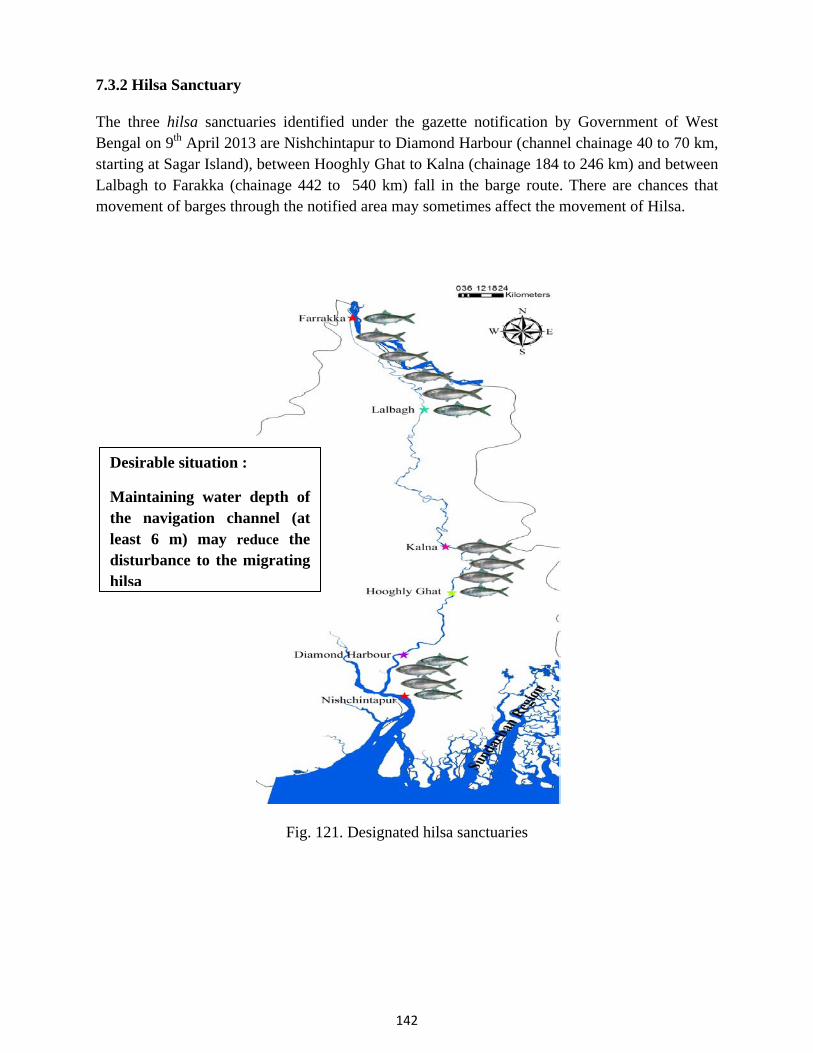
142
7.3.2 Hilsa Sanctuary
The three hilsa sanctuaries identified under the gazette notification by Government of West Bengal on 9th April 2013 are Nishchintapur to Diamond Harbour (channel chainage 40 to 70 km, starting at Sagar Island), between Hooghly Ghat to Kalna (chainage 184 to 246 km) and between Lalbagh to Farakka (chainage 442 to 540 km) fall in the barge route. There are chances that movement of barges through the notified area may sometimes affect the movement of Hilsa.
Fig. 121. Designated hilsa sanctuaries
Desirable situation :
Maintaining water depth of the navigation channel (at least 6 m) may reduce the disturbance to the migrating hilsa

143
7.4 Densely populated areas The studied stretch include two intensely populated cities of Kolkata and Howrah. The agglomerated cities / townships extend from Diamond Harbour in the downstream to Nabadwip in the upstream. A significant area is having different types of industries like jute, paper, tannery etc. 7.5 Natural hazards The lowermost part is highly prone to different natural calamities. Cyclonic events are quite common in this region especially in the months of May-June. A recent such heavy cyclonic storm named ‘Aila’ did lot of destruction in lower region of Hooghly-Matlah estuary especially in Sundarban. During August-September, water used to come in more vigour during high tide (bore tide, locally known as Ban). The tidal bore is well known to affect the shipping and navigation in the estuarine zone of river Hooghly. 7.6 Delineation of saline zone During pre-Farakka barrage (before 1975), water flow was much less through Bhagirathi- Hooghly river system. Accordingly, effect of saline water intrusion during high tide was felt even at Barrackpore (Nawabganj) with salinity up to 1.16 ppt (Fig. 122). However, increase in freshwater discharge in post-Farakka period increased the length of freshwater stretch downwards up to Godakahli (between Uluberia and Burul). Accordingly distribution and fish species availability was also thoroughly modified. Details of the salinity based zonation and its effect on fish species distribution was recently reviewed by Manna et al. (2013).
Fig. 122. Salinity map of river Hooghly during pre- and post- Farakka period
(Source: Manna et al., 2013)

144
The variations in fish species distribution with change in salinity is presented in Fig. 123. There are 17 fish species which are distributed everywhere irrespective of change in salinity.
Fig. 123. Euryhaline fish species reported from River Hooghly
(Source: CIFRI Annual Report, 2010-11)
Saline
Freshwater Zone
Transition
17species
104species
3species
66species
14 species
25species
0species
Euryhaline Fish species
1. Apocryptis bato 2. Brachygobius nunus 3. Cynoglossus cynoglossus 4. Eleotris fusca 5. Euryglossa pan 6. Glossogobius giuris 7. Hyporhampus limbatus 8. Johnius coitor 9. Johnius gangeticus 10. Odontamblyopus rubicundus 11. Otolithoides pama 12. Pangasius pangasius 13. Pisodonophis boro 14. Pseudapocryptes elongates 15. Rhinomugil corsula 16. Setipinna phasa 17. Tenualosa ilisha

145
8.0 Probable Impacts and Recommendations
8.1 Probable Impacts
Movement of coal laden barges may lead to impact on the following aspects
Pollution and spillage
The company, presently involved in transportation of coal through the barges, M/s Jindal ITF Ltd. has stated that it is following Standard Operating Procedures (SOPs) to prevent spillage of oil/ fuel/ grease, coal and other pollutants from the barge during the operation and also in emergencies. Details of SOP as provided by the company are described under item 3 of this report. However, in case of accidents if oil and grease spills, it will adsorb on the surface of the biota and will reduce the respiration and photosynthetic efficiencies. Some spillage of coal was recorded at the unloading point at Farakka (Station Farakka 2) initially, which was not recorded during visit by CIFRI Team subsequently.
Habitat parameters
The study revealed that the movement of barges increases water turbidity and alters river flow. About 10% increase in turbidity has been recorded in shallower areas and bank areas due to movement of barges. Increased water turbidity will reduce primary production and will ultimately reduce the energy flow through the aquatic food chain.
Fisheries
In the upper zone (Zone III : Nabadwip to Farakka) fishermen generally use the gill nets of varying sizes. In the lower zone (Zone I : Sagar Island to Dakshineswar) bag nets along with gill nets are predominant. The fishermen possess around 10-15 nets of different types and boat/dingy for fishing operation. In the upper zone they use traps also. The fishermen do fishing for 5-12 hours daily, depending upon the season and maximum fishing activities take place during night, morning and evening hours, especially along the upper stretch. Lower stretch is comparatively wider; fishermen are able to avoid the barges and ships while fishing. Zone III being narrow, there is disturbance to the existing fishing operations during barge movement. It has been observed that on an average, the movement of barges is affecting the fishing operations by about 20 minutes per day. Few cases of damage of fishing nets have been observed particularly from the upper (zone III, Nabadwip to Farakka) and middle (zone II, Dakshineswar to Nabadwip) stretches.
The three hilsa sanctuaries identified under the gazette notification by Government of West Bengal on 9th April 2013 are Nishchintapur to Diamond Harbour (channel chainage 40 to 70 km, starting at Sagar Island), between Hooghly Ghat to Kalna (chainage 184 to 246 km) and between Lalbagh to Farakka (chainage 442 to 540 km) fall in the barge route. There are chances that movement of barges through the notified area may sometimes affect the movement of Hilsa.

146
Bottom biota
It has been observed that the movement of barges and their propeller wash disturb the bottom sediment, along with the associated fauna, especially in shallower areas. This may also disturb the breeding and feeding grounds of several bottom dwelling organisms.
Impact on other aquatic species
The river stretch is a known habitat for Gangetic dolphin (Platanista gangetica gangetica) and common otter, Lutra lutra (locally known as Bhodar / Udbiral). It is anticipated that there may be some effect of barge movement on dolphin and otter especially in the narrow stretches. Fast moving vessels may directly hit calves and carrying mothers especially in narrow stretches of the river.
Aquatic and shore line macro vegetations
Increased wave actions on the banks, especially in curved and narrow stretches, due to movement of barges may accelerate erosion in the above stretches affecting the macrophyte vegetation and associated fauna.
Bank erosion
It has been observed that out of 545 km of the studied stretch (Sagar Island to Farakka), 185 km stretch is vulnerable to erosion due to barge movement. There is possibility of acceleration in the erosion due to barge movement in narrow and curved stretches.
Passenger ferry boat operations
In addition to the fishing boats, passenger ferry boats also operate in the studied stretch. In some stretches the intensity of ferry operation is one in every kilometer. There is chance that both are affected due to operation of the barges.

147
8.2 Recommendations
Based on the investigations made during the pre-monsoon and monsoon periods (March to August, 2014) on the impacts of movement of coal laden barges on aquatic flora and fauna in the river Bhagirathi-Hooghly (Sagar Island to Farakka), the following recommendations are drawn :
• Precautionary measures viz., use of better/ fool proof handling equipments, transportation of coal in closed barges to be strictly followed to ensure zero spillage of coal particles during loading, transport and unloading. In addition, strict measures to be implemented to prevent spillage/leakage of oil and grease at filling, handling and servicing points of vessels in order to protect environment, and biota. Care should be taken so that the sewages and garbage generated are disposed at designated sites only after necessary treatment.
• The vessels should navigate only through the designated navigation channel and the channels need to be indicated through beacons. Electronic Navigational Chart is provided by IWAI which is updated regularly through river notices. These should be strictly followed.
• During night operations, the barges should use powerful search lights and horns so as to warn the fishers of the incoming barges well in advance at least from 500 m away.
• In case of damage of fishing nets, fishing crafts and other gears of fishers, arising due to barge operation, appropriate and quick compensations may be given to the aggrieved fishers.
• Reducing speed of barges in the curved and narrow stretches from its normal speed of 7-8 nautical miles/h to 5-6 nautical miles/h is recommended for reducing the wave action and thereby minimizing possibilities of bank erosion. Some of the critical, curved areas of the river are lying between the channel chainage from 256 to 274 km; 310 to 324 km; 400 to 410 km; 448 to 462 km; 474 to 492 km from the Sagar Island (origin), where the speed of barges to be maintained at or below 5-6 nautical miles/h for reducing chances of erosion. The critically erosion prone zones need to be protected through erection of retaining walls, putting gabions with stones, stone pitching, establishing vegetation, etc.
• Maintaining water depth of the navigation channel (at least 6 m) may reduce the disturbance to benthic habitat, facilitate escapement of fishes and aquatic mammals from direct impact of the barge, considering that the fully loaded barge draft is 2.7 m. This will also help hilsa, which prefers more than 5 m depth for their migration.
• Preparation and publishing barge movement schedule, pre-signaling of movement, fixed timing, generation of awareness on barge movement among public, specifically the fishers and ferry operators may be made.
• There may be 24 hour functional dedicated disaster management cells/ control rooms established along the stretch of the barge movement, apart from the control room established by Jindal ITF for monitoring movement of barges, to deal with emergencies.
• Since the barge movement started recently, follow up investigations are necessary to keep track of any impact for ensuring early amelioration measures by establishing a mechanism for regular monitoring of the recommended measures as well as the impact on the environment and biota.

148
• As per available information, inland navigation is considered as one of the most environmentally sound and sustainable forms of transport. However, awareness among the fishers and public on the matter is poor. Therefore there is need for generating awareness about the IWAI navigation channel designated in the year 1986 for use as means for transport.

149
References 1. Ahmed, M.F., Yusoff, M. M., Husain, M. L., Wan Nik, W. M. M., & Muzathik, A. M (n.d). 1989.
An investigation of boat wakes wave energy: a case study of Kemaman River Estuary, 907-913. Retrieved from http://umt.edu.my
2. Anand, N., 1998. Indian Freshwater microalgae. Bishen Singh Mahendra Pal Singh, DehraDun, India, 94p.
3. APHA, 2012. Standard methods for the examination of water and wastewater. 22nd edition. APHA, AWWA & WEF, Springfield, New York, Washington.
4. Arlinghaus, R., Engelhardt, C., Sukhodolov, A. and Wolter, C. 2002. Fish recruitment in a canal with intensive navigation: implications for ecosystem management. J. Fish Biol. 61: 1386-1402.
5. Baldwin, D. S. 2008. Impacts of recreational boating on river bank stability: Wake characteristics of powered vessels. Report for the Murray Catchment Management Authority. Murray-Darling Freshwater Research Centre, Wodonga, Victoria. Retrieved from http://arrow.latrobe.edu.au
6. Bartell, S. M. and Campbell, K. R. 2000. Ecological Risk Assessment of the Effects of the Incremental Increase of Commercial Navigation Traffic (25, 50, 75, and 100 Percent Increase of 1992 Baseline Traffic) on Fish. U.S. Army Corps of Engineers, Upper Mississippi River – Illinois Waterway System Navigation Study, ENV Report 16. 132 pp.
7. Battish, S. R. 1992. Freshwater zooplankton of India. Oxford and IBH publishing Co. Pvt. Ltd. New Delhi. India. p 233.
8. Bauer, B. O., Lorang, M. S., & Sherman, D. J. (2002). Estimating boat-wake-induced leveeerosion using sediment suspension measurements. Journal of Waterway, Port, Coastal, and Ocean Engineering, 128(4), 152–162. doi:10.1061/(ASCE)0733-950X(2002)128:4(152)
9. Bauer, B.O., Lorang, M.S., Sherman, D.J., 2002. Estimating boat-wake-induced levee erosion using sediment suspension measurements. Journal of Waterway, Port, Coastal and Ocean Engineering 128, 152−162.
10. Baykal, T., Açikgöz, I., Udoh, A. U. and Yildiz, K. 2011. Seasonal variations in phytoplankton
composition and biomass in a small lowland river-lake system (Melen River, Turkey). Turk. J. Biol.,
35: 485-501.
11. Baykal, Tülay, İlkay Açikgöz, Abel U. Udoh and Kazım Yildiz, 2011. Seasonal variations in phytoplankton composition and biomass in a small lowland river-lake system (Melen River, Turkey). Turk J Biol., 35, 485-501.
12. Beachler, M. M., & Hill, D. F. (2003). Stirring up Trouble? Resuspension of bottom sediments by recreational watercraft. Lake and Reservoir Management, 19(1), 15–25.
13. Bhaumik, U. and Sharma, A. P. 2012. Present status of hilsa in Hooghly-Bhagirathi river. CIFRI Bulletin No. 179. p 35.
14. Bhaumik, U., Srivastava, N. P., Satpathy, B. B., Mukhopadhyay, M. K. and Sharma, A. P. 2011. Impact of hydro-ecology on fish migration in selected east coast estuaries. J. Inland Fish. Soc. India 43(1): 1-9.
15. Bhowmik, N. G., Demissie, M., & Osakada, S. (1981). Waves and drawdown generated by river traffic on the Illinois and Mississippi Rivers. SWS Contract Report 271, Illinois Institute of Natural Resources, University of Illinois, Champaign. Retrieved from http://isws.illinois.edu.
16. Biggs, B .J. F. and Kilroy, C. 2000. Taxonomic analysis. In: Stream Periphyton monitoring manual. NIWA, Christchurch, New Zealand, 95-111 pp.

150
17. Bonham, A. J. (1983). The management of wave-spending vegetation as bank protection against boat wash. Landscape Planning, 10(1), 15–30.
18. Bradbury, J. 2005 Revised wave wake criteria for vessel operation on the lower Gordon River criteria revision report. Unpublished Nature Conservation Branch report, DPIWE.
19. Chadwick J. W. and Steven P. Canton, 1983. Coal mine drainage effect on a lotic ecosystem in North West Colorado, U.S.A., Hydrobilogia, 107: 25-33.
20. Cherry, D. S., Guthrie, R. K., Sherberger F. F. and Larrick, S. R. 1979a. The influence of coal ash and thermal discharges upon the distribution and bioaccumulation of aquatic invertebrates. Hydrobiologia 62: 257–267.
21. Chovance, A., Hoffer, R. and Schiemer, F. 2003. Fish as bioindicators. In Market, B. A., Breure, A. M., Zechmeiser, H. G. (eds) Bioindicatos and biomonitors, pp 639–675.
22. Civco D.L, Hurd J.D., Wilson E.H., Song M., Zhang Z., 2002. A comparison of land use and land cover change detection methods. In: Proceedings, 2002 ASPRS-ACSM Annual Conference and FIG XXII Congress,Washington, DC, April 22–26. Bethesda, MD: American Society for Photogrammetry & Remote Sensing, pp 22–26.
23. Colvile, R. N., Hutchinson, E. J., Mindell, J. S. and Warren, R. F. 2001. The transport sector as a source of air pollution. Atmospheric Environment 35: 1537–1565.
24. Cox, E. J. 1996. Identification of fresh water diatoms from live material. Chapman & Hall, London, UK. 158p.
25. CPCB. 2009. Central Pollution Control Board report on “Ganga water quality trend” 2009. 26. CPCB. 2013. Central Pollution Control Board report on “Pollution assessment : river Ganga” 2013. 27. Crosato A. 1990. Simulation of meandering river processes. In Communications on Hydraulic and
Geotechnical Engineering. Delft University of Technology: Delft, The Netherlands. 28. Darby SE, Thorne CR. 1996. Development and testing of riverbank-stability analysis. Journal of
Hydraulic Engineering 122(8): 443–454. 29. Darwall, W. R. T. and Vie, J. C. 2005. Identifying important sites for conservation of freshwater
biodiversity: extending the species based approach. Fish. Manag. Ecol. 12: 287–293. 30. David, A. 1954. A preliminary survey of the fish and fisheries of a five mile stretch of Hooghly
river near Barrackpore. Indian J. Fish. 1(1 & 2): 231-255. 31. Deksne, R., Škute, A., Meinerte, A. 2011. Seasonal changes in zooplankton community of the
Daugava River. Acta Biologica Universitatis Daugavpiliensis 11 (1): 61-75. 32. Dorak Zeynep, 2013. Zooplankton abundance in the lower Sakarya River Basin (Turkey): Impact of
environmental variables. J. Black Sea/Mediterranean Environment 19(1): 1-22. 33. Dorava, J. M., & Moore, G. W. (1997). Effects of boatwakes on streambank erosion, Kenai River,
Alaska. USGS Water-Resources Investigations Report, 84. Retrieved from http://ak.water.usgs.gov 34. Dorava, J. M., & Moore, G. W. (1997). Effects of boatwakes on streambank erosion, Kenai River,
Alaska. USGS Water-Resources Investigations Report, 84. Retrieved from http://ak.water.usgs.gov 35. Downing, J.P., Sternberg, R.W. and Lister, C.R.B. 1981 New instrumentation for the investigation of
sediment suspension processes in the shallow marine environment. Marine Geology. 42: 19 -34. 36. Duchrow, R. M. 1982. Effects of barite tailings on benthos and turbidity of two Ozark streams.
Transactions of the Missouri 37. Dudgeon, D., Arthington, A. H., Gessner, M. O., Kawabata, Z. I., Knowler, D. J., Leveque, C.,
Naiman, R. J., Prieur-Richard, A. H., Soto, D., Stiassny, M. L. J. and Sullivan, C. A. 2006. Freshwater biodiversity: importance, threats, status and conservation challenges. Biol. Rev. 81: 163–182.
38. Edmondson, E.T. 1959. Freshwater biology. John Wiley &Sons, Inc. Ney York. p1248. 39. European Commission. 2000. WHITE PAPER – European Transport Policy for 2010: Time to
Decide. Office for Official Publications of the European Communities, Luxembourg. 119 pp.

151
40. Gao Y, Mas JF, Niemeyer I, Marpu PR, Palacio JL. 2007. Object based image analysis for forest area land cover mapping. In: Proceedings, International Symposium for Spatial Data Quality (ISSDQ). Enschede, the Netherlands, 13–15 June, 2007. Enschede, the Netherlands: ISSDQ 2007 Secretariat. http://www.itc.nl/ISSDQ2007/proceedings/index.html; accessed on 21 April 2010.
41. Garrard, P.N. and Hey, R.D. 1987 Boat traffic, sediment resuspension and turbidity in a Broadland river. Journal of Hydrology. 95: 289 - 297.
42. Glamore, W.C., 2008. A decision support tool for assessing the impact of boat wake waves on inland waterways. On Course 133, October 2008.
43. Guiry, M. D. and Guiry, G. M. 2013. AlgaeBase. World-wide electronic publication, National University of Ireland, Galway. http://www.algaebase.org; searched on 30 November 2013
44. Guthrie, R. K., Cherry, D. S. and Singleton, F. L. 1978. Responses of heterotrophic bacterial populations to pH changes in coal ash effluent. Water Resource Bulletin 14: 803–808.
45. Gutreuter, S., Dettmers, J.M. and Wahl, D.H. 2003. Estimating mortality rates of adult fishes from entrainment through the propellers of river towboats. Trans. Am. Fish. Soc. 132: 647–661.
46. Hall, E.M. 1997. Detetrmination of trace elements in sediments In A. Mudroch, J. M. Azcue and P. Mudroch (eds.) Manual of physicochemical analysis of aquatic sediments. Lewis publishers,USA.pp.85 – 145
47. Harken J., Sugumaran R. ,2005. Classification of Iowa wetlands using an airborne hyperspectral image: A comparison of spectral angle mapper classifier and an object-oriented approach. Canadian Journal of Remote Sensing 31(2): 167–174.
48. Holland, L.E. 1986. Effects of barge traffic on distribution and survival of ichthyoplankton and small fishes in the Upper Mississippi River. Trans. Am. Fish. Soc. 115: 162–165.
49. Holland, L.E. and Sylvester, J.R. (1983) Distribution of larval fishes related to potential navigation impacts on the Upper Mississippi River, Pool 7. Trans. Am. Fish. Soc. 112, 293–301.
50. Hooke JM. 1995. River channel adjustment to meander cutoffs on the River Bollin and River Dane. Geomorphology 14: 235–253.
51. Hora, S. L. 1943. Evidence of distribution of fishes regarding rise in salinity of the river Hooghly. Current Science 3: 89-90.
52. Houser, C., 2011. Sediment resuspension by vessel-generated waves along the Savannah River, Georgia. Journal of Waterway, Port, Coastal, and Ocean Engineering. doi:10.1061/(ASCE)WW.1943-5460.0000088.
53. http:/www.cag.gov.in/reports/ scientific/ 2000 book2 /gangaactionplan. htm, http:/www.gits4u.com/water/ganga.htm
54. Huckstorf, V., Lewin, W., Mehner, T. and Wolter, C. 2010. Impoverishment of YOY-fish assemblages by intense commercial navigation in a large Lowland river. River Research and Applications, 27(10): 1253-1263.
55. Hüsig, A., Linke, T. and Zimmermann, C. 2000. Effects from supercritical ship operation on inland canals. J. Waterway, Port, Coastal, Ocean Eng. 126: 130–135.
56. Hustedt, F., 1976. Bacillariophyta (Diatomeae). Verlag Von Gustab Fischlp, Germany, 466p. 57. IIT, 2012. Floral and Faunal Diversity in Lower Ganga Farakka to Gangasagar. GRB EMP : Ganga
River Basin Environment Management Plan, Report code: 027_GBP_IIT_ENB_DAT_04_Ver_Jun 2012. p 48.
58. Ikeda S, Parker G, Sawai K. 1981. Bend theory of river meanders, 1, Linear development. Journal of Fluid Mechanics 112: 363–377.
59. Johannesson H. 1985. Computer Simulation of Migration of Meandering Rivers. Dissertation, University of Minnesota, St. Paul.
60. Jude, D. J., Tesar, F. J. and Tin, H. T. 1998. Spring distribution and abundance of larval fishes in the St. Marys River, with a note on potential effects of freighter traffic on survival of eggs and larvae. J. Great Lakes Res. 24: 569–581.

152
61. Kang, B., He, D., Perrett, L., Wang, H., Hu, W., Deng, W. and Wu, Y. 2009. Fish and fisheries in the Upper Mekong: current assessment of the fish community, threats and conservation. Rev. Fish. Biol. Fish., 19:465–480
62. Kar, D, Sur, P., Mandal, S. K., Saha, T. and Kole, R. K., 2008. Assessment of heavy metal pollution in surface water. Int. J.Environ. Sci. Tech. 5(1), 119–124.
63. Karr, J. R. and Chu, E. W. 1999. Restoring Life in Running Waters. Island Press, Washington, D.C. 206 pp.
64. Khan, N. I., and A. Islam. 2003. Quantification of erosion patterns in the Brahmaputra-Jamuna River using geographical information system and remote sensing techniques. Hydrological Processes 17, 959 - 966.
65. Killgore, K. J., Maynord, S. T., Chan, M. D. and Morgan II, R. P. 2001. Evaluation of propeller-induced mortality on early life stages of selected fish species. North Am. J. Fish. Mgmt. 21, 947–955.
66. Kirkegaard, J., Kofoed-Hansen, H., & Elfrink, B. (1998). Wake wash of high-speed craft in coastal areas. Coastal Engineering Proceedings, 1(26), 325–337.
67. Kubec, J. and Podzimek, J. 1996. Wasserwege. Verlag Werner Dausien, Hanau. 491 pp. 68. Laffaille, P., Acou, A., Guillouet, J., Legult, A. 2005. Temporal change in European eel, Anguilla
anguilla, stock in a small catchment after installation of fish passes. Fish. Manag. Ecol. 12:123–129. 69. Lal, B. 1990. Impact of Farakka barrage on the hydrological changes and productivity potential of
Hooghly estuary. J. Inland Fish Soc. India 22(1 & 2): 38-42. 70. Larissa Laderoute & Bernard Bauer 2013 River bank erosion and boat wakes along the lower
shuswap river, british columbia final project report submitted to Regional District of North Okanagan Fisheries and Oceans Canada University of British Columbia Okanagan
71. Macfarlane, G. J., Bose, N., & Duffy, J. T. (2012). Wave wake: Focus on vessel operations within sheltered waterways. In 2012 SNAME Annual Meeting & Exposition and Ship Product Symposium, 1, 27–48.
72. Manna, R. K., Satpathy, B. B., Roshith, C. M., Naskar, M., Bhaumik, Utpal and Sharma, A. P. 2013. Spatio-temporal changes of hydro-chemical parameters in the estuarine part of the river Ganges under altered hydrological regime and its impact on biotic communities. Aquatic Ecosystem Health & Management, 16(4): 433-444.
73. Marneffe, Y., Descy, J. P., Thomé, J. P. 1996. The zooplankton of the lower river Meuse, Belgium: seasonal changes and impact of industrial and municipal discharges. Hydrobiologia 319: 1-13.
74. Maynord, S. T., Biedenharn, D. S., Fischenich, C. J., & Zufelt, J. E. (2008). Boat-wave-induced bank erosion on the Kenai River, Alaska. Retrieved from http://dtic.mil
75. Mitra, P. M., Ghosh, K. K., Saigal, B. N., Sarkar, N. D., Roy, A. K., Mondal, N. C. and Paul, A. R. 1987. Fishing gear of the upper and the middle Hooghly estuary. Bulletin no 49. CIFRI, Barrackpore, 22p.
76. Mitra, P. M., Karmakar, H. C., Ghosh, A. K., Mandal, N. C., Sen, H. K. and Das, B. N. 2001. Fisheries of Hooghly Matlah estuarine system – further appraisal. Bulletin no 109. CIFRI, Barrackpore, 18p.
77. Mueller, G. 1980. Effects of recreational river traffic on nest defence by longear sunfish. Trans. Am. Fish. Soc. 109: 248–251.
78. Mukherjee, D. P. 2012. Global Perspective of monitoring metal ions in Ganges river – A case Study. Arch. Appl. Sc. Res. 4(2): 1007–1021
79. Nandy, A. C., Bagchi, M. M. and Majumder, S. K. 1983. Ecological changes in the Hooghly estuary due to water release from Farakka barrage. Mahasagar 16(2): 209-220.
80. Nath, D., Misra, R. N. and Karmakar, H. C. 2004. The Hooghly estuarine system – Ecological flux, fishery resources and production potential. Bulletin no 130. CIFRI, Barrackpore, 47p.

153
81. Newman, J.N., 1977. Marine Hydrodynamics. MIT Press. 82. Nielsen, L.A., Sheehan, R.J. and Orth, D.J. 1986. Impacts of navigation on riverine fish production
in the United States. Pol. Arch. Hydrobiol. 33: 277–294. 83. Odgaard A. 1989a. River meander model, I: Development. Journal of Hydraulic Engineering
115(11): 1433–1450. 84. Odgaard A. 1989b. River meander model, II: Application. Journal of Hydraulic Engineering
115(11): 1450–1464. 85. Odom, M.C., Orth, D.J. and Nielsen, L.A. 1992. Investigation of barge-associated mortality of larval
fishes in the Kanawha River. Virginia J. Sci. 43, 41–45. 86. Oregon State Marine Board. (2003). Watching Your Wake: A Boater’s Guide. Pamphlet. Retrieved
from http://cms.oregon.gov 87. Osman MA, Thorne CR. 1988. Riverbank stability analysis. I: Theory. Journal of Hydraulic
Engineering 114(2): 134–150. 88. Parnell, K. E., Mcdonald, S. . C., & Burke, A. E. (2007). Shoreline effects of vessel wakes,
Marlborough Sounds, New Zealand. Journal of Coastal Research, 50, 502–506. 89. Parnell, K. E., Mcdonald, S. . C., & Burke, A. E. (2007). Shoreline effects of vessel
wakes,Marlborough Sounds, New Zealand. Journal of Coastal Research, 50, 502–506. 90. Philipose, M.T., 1967. Chlorococcales. Indian Council of Agricultural Research, New Delhi. 364 p. 91. Prescott, G. W. 1899. Algae of the western Great Lakes area, with an illustrated key to the genera
of desmids and freshwater diatoms. Dubuque, Iowa,W. C. Brown Co. 1000p. 92. Pygott, J. R., O’Hara, K. and Eaton, J. W. 1990. Fish community structure and management in
navigated British canals. In: van Densen, W.L.T., Steinmetz, B. and Hughes, R.H. (eds.), Management of Freshwater Fisheries. Pudoc, Wageningen, pp. 547–557.
93. Ramanathan, K. R., 1964. Ulotrochales. Indian Council of Agricultural Research, New Delhi. 188p. 94. Reynolds C.S., 2006. Ecology of phytoplankton. Cambridge Univ. Press; Cambridge. 95. Samanta, S. 2013. Metal and pesticide pollution scenario in Ganga River system.Aquatic Ecosystem
Health and Management.16 (4): 454–464. 96. Samanta, S., Chandra, K., Manna, S. K. and Saha, K. 2007.Sediment status of the Hooghly and
Haldi estuaries at Haldia industrial area with special reference to trace metals. J. Indian Soc. Soil Sc. 55(3): 349-359.
97. Sarkar, S. K, Saha M., Takada H., Bhattacharya A., Mishra P. and Bhattacharya B., 2007. Water Quality management in the lower stretch of the river Ganges, east coast of India: an approach through environmental education. J. Clean. Prod. 15(16), 1559–1567.
98. Sarkar, U. K, Pathak, A. K. and Lakra, W. S. 2008. Conservation of freshwater fish resources of India: new approaches, assessment and challenges. Biodivers. Conserv. 17: 2495–2511.
99. Sarma, V. V., Sudhakar, U. and Varaprasad, S. J. D. 1993. Behaviour of fluoride and dissolved silicon in Goutami Godavari estuarine environment. Mahasagar 26(2): 105-113.
100. Seegers, L., Vos, L. D., Okeyo, D. O. 2003. Annotated checklist of the freshwater fishes of Kenya (excluding the lacustrine haplochromines from Lake Victoria). Journal of East African Natural History 92(1):11-47.
101. Sharma, S., Siddique, A., Singh, K., Chouhan, M., Vyas, A., Solnki, C. M., Sharma, D., Nair, S., Sengupta, T. 2010. Population dynamics and seasonal abundance of zooplankton community in Narmada River (India). Researcher 2 (9): 1-9.
102. Sheremet, A., Gravois, U., & Tian, M. (2012). Boat-wake statistics at Jensen Beach, Florida. Journal of Waterway, Port, Coastal, and Ocean Engineering. doi:10.1061/(ASCE)WW.1943-5460.0000182
103. Shetty, H. P. C. Saha S. B. and Ghosh B. B.. 1956. Observations on the distribution and fluctuations of plankton in the Hooghly-Matlah estuarine system, with notes on their relation to commercial fish landings. Indian Journal of Fisheries 8(2): 326-363.

154
104. Simmonds, M., Dolman, S. and Weilgart, L. 2004. Oceans of Noise. Science report prepared by the Whale and Dolphin Conservation Society (WDCS). Chippenham, United Kingdom. 168pp.
105. Simmonds, M.P. and Lopez-Jurado, L.F. 1991. Whales and the military. Nature 351(6326):448. 106. Slabbekoorn, H., Bouton, N., van Opzeeland, I., Coers, A., ten Cate, C., Popper, A. N., 2010. A
noisy spring: the impact of globally rising underwater sound levels on fish. Trends. Ecol. Evol.;25(7): 419-27.
107. Stephen T. Maynord, David S. Biedenharn, Craig J. Fischenich, and Jon E. Zufelt 2008 Boat-Wave-Induced Bank Erosion on the Kenai River, Alaska Final report Approved for public release; distribution is unlimited. ERDC TR-08-5
108. Summarwar, S. 2012. Studies on plankton diversityin Bisalpur reservoir, Int. J. LifeSc. Bt& Pharm. Res. 1:(4).
109. Sun T, Meakin P, Jossang T. 2001a. A computer model for meandering rivers with multiple bedload sediment sizes. 1. Theory. Water Resources Research 37(8): 2227–2241.
110. Tiwari S K. 1999. Animal kingdom of the World, vol.1. Fundamentals of world 111. United Nations. 1997. Kyoto Protocol to the United Nations Framework Convention on Climate
Change. United Nations, New York, FCCC/CP/1997/L.7/Add.1. 20 pp. 112. USEPA. 2011. The effects of mountaintop mines and valley fills on aquatic ecosystems of the
Central Appalachian coalfields. Office of Research and Development, National Center for Environmental Assessment, Washington, DC. EPA/600/R-09/138F.
113. Vass, K. K.; Samanta, S.; Suresh, V. R.; Katiha, P. K. And Mandal, S. K. 2008. Current status of river Ganges. Bull No. 152. Central Inland Fisheries Research Institute, Barrackpore. p 34.
114. Witty Lynne M., 2004. Practical Guide to Identifying Freshwater Crustacean Zooplankton. 2nd edition. Cooperative Freshwater Ecology Unit Department of Biology, Laurentian University. Ontario, Canada, p 50.
115. Wolter, C. 2001. Conservation of fish species diversity in navigable waterways. Landscape and Urban Planning 53: 135–144.
116. Wolter, C. and Arlinghaus, R. 2003. Navigation impacts on freshwater fish assemblages: the ecological relevance of swimming performance. Reviews in Fish Biology & Fisheries 13: 63–89.
117. Wolter, C. and Vilcinskas, A. 1997. Perch (Perca fluviatilis) as an indicator species for structural degradation in regulated rivers and canals in the lowlands of Germany. Ecol. Freshw. Fish 6: 174–181.
118. Yoon GW, Cho SI, Chae GJ, Park JH. 2004. Automatic land-cover classification of Landsat images using feature database in a network. International Archives of Photogrammetry Remote Sensing and Spatial Information Sciences 35(2): 564–568.
119. Yousef, Y. A., Mclellon, W. M., & Zebuth, H. H. (1980). Changes in phosphorus concentrations due to mixing by motorboats in shallow lakes. Water Research, 14, 841–852.
120. Zauner, G. and Schiemer, F. 1992. Auswirkung der Schiffahrt auf die Fischfauna – aufgezeigt am Beispiel der österreichischen Donau. Landschaftswasserbau 14: 133–152.
Zauner, G. and Schiemer, F. 1994. Auswirkung der Schiffahrt auf die Fischfauna großer Fließgewässer. Wiss. Mitt. Niederösterr. Landesmuseum 8: 271–285.

155
ANNEXURE I

156

157

158

159

160

161
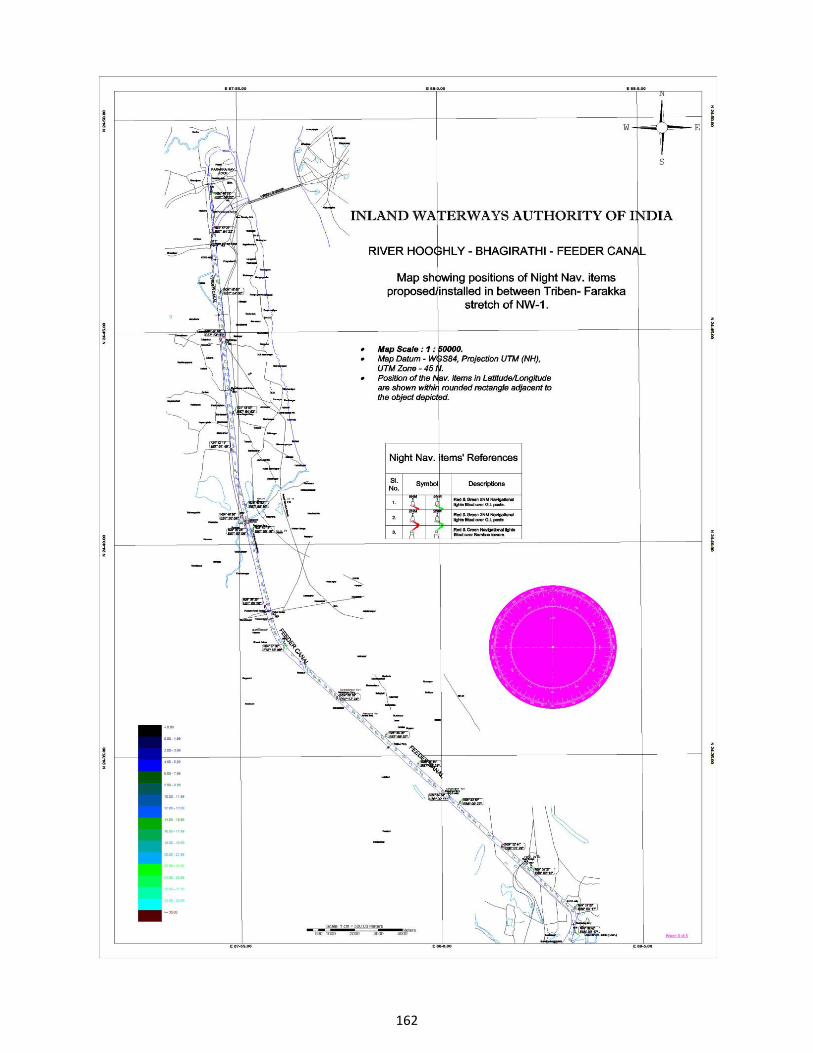
162

163
INDEX I
Alkalinity, 28, 29, 36, 37 Ammonia, 34 Amphidromous, 76 Anadromous, 75 Aquatic macrophyte, 59,60 Associated fauna, 23, 60, 146 Available nitrogen, 33, 40, 43, 44 Awareness, 19, 98, 147, 148 Bank erosion, 3, 24, 59, 99, 107, 114, 115, 116,
117, 119, 120, 130, 132, 133, 146, 147 Bank profile, 133 Barge wakes, 99, 100, 128, 129, 130, 131, 133 Bathymetry, 103, 116, 117, 122, 127, 132, 137 Benthic, 2, 23, 38, 55, 56, 57, 58, 147 Biochemical Oxygen Demand, 31, 32, 36, 37 Bottom biota, 146 Brush mattress, 136 Bunkering, 15 Carrying capacity, 14 Catadromous, 75, 76 Check dams, 134 Chemical oxygen demand, 32, 33 Clay, 26, 38, 43, 44, 117, 120, 130, 133 Coal Handling Plant, 14, 15, 18, 20 Coal requirement, 1 Coal slurry management, 17 Coir geo textile rolls (CGR), 135 Crafts, 18, 82, 85, 86, 147 Critical speed 24, 123, 125, 126 Cruising speed, 125 Densely populated areas, 143 Deposition, 55, 59, 99, 100, 112, 114, 115, 133 Disaster management, 18, 19, 147 Displacement speed, 127, 132 Semi-displacement speed, 127, 128 Dissolved oxygen, 26, 27, 31, 32, 36, 37, 131 Divergent waves, 99, 124, 125, 126 Dolphin, 139, 140, 141, 146 Dust suppression system, 16, 17 Ecologically important areas, 138 Erosion, 3, 24, 59, 85, 86, 99, 100, 101, 107,
110, 111, 112, 114, 115, 116, 117, 119, 120, 121, 124, 128, 129, 130, 131, 132, 133, 134, 135, 137, 146, 147
Fishermen, 2, 3, 19, 62, 82, 85, 86, 87, 89, 90,139, 145
Fish breeding, 74 Fish species, 2, 3, 23, 62, 68, 69, 70, 71, 72, 74,
76, 95, 143, 144 Fishers’ perception, 85, 86, 87 Fishing gears, 24, 82, 85, 91 Flow, 1, 3, 23, 34, 45, 59, 60, 62, 74, 76, 92,
99, 100, 102, 103, 104, 105, 108, 114, 115, 116, 117, 118, 119, 120, 122, 130, 132, 133, 134, 136, 137, 143, 145
Free CaCO3, 39, 43, 44 Free CO2, 28, 36, 37 Froude number, 122, 123, 125, 126, 127 Gabion, 134, 135, 147 Garbage / Garbage management, 14, 147 GIS, 110, 111, 112, 114 Grab un-loader, 15, 16 Hardness, 29, 30, 36, 37 Hilsa, 75, 84, 89, 91, 92, 93, 94,95, 96, 142, 145,
147 Hilsa fishery, 89 Hilsa sanctuary, 142 Hoppers, 16, 17 Hump speeds, 127 Ichthyofauna, 62, 67, 70, 73, 76 Imported coal, 1, 14 IUCN Red List, 72, 73 IWAI, 1, 3,4, 6, 18, 19, 147, 148 Jindal ITF, 1, 13, 15, 18, 19, 56, 145, 147 Kanika Sands, 1, 5, 13 Kelvin wave pattern, 123, 124 Major constraints, 87 Management of the pollutants, 14 Metal contaminations, 77, 78, 79, 80 Migration, 23, 25, 74, 75, 76, 91, 99, 114, 115,
147 MoEF, 1 Monthly expenditure, 83, 84 Monthly income, 83, 84 National Waterway No.1, 1, 4, 5, 6, 7, 8, 9, 10,
11, 12, 138 Natural hazards, 143 Navigation channel, 25, 81, 147, 148 Navigational Chart, 19, 147

164
NH4, 33, 34, 36, 37, 40, 102, 104 Night operations, 147 Nitrogen, 33, 34, 40, 41, 43, 44 NO3, 33, 34, 40, 102, 104, 105 NTPC, 1, 3, 13, 17, 81 Number of fishermen, 89 Ocean Going Vessels, 13 Oil management, 14 Organic carbon, 28, 40, 43, 44 ORP, 102, 104, 105 Otter, 139, 146 Passenger ferry boats, 146 Phosphorus, 28, 33, 38, 41, 43, 44, 150, 154 Physico-chemical features, 24, 38 Physico-chemical parameters, 36, 37, 43, 44 Phytoplankton, 1, 45, 46, 47, 49, 50, 54 Planing speed, 132 Plankton, 23, 26, 27, 28, 33, 40, 45, 54 PO4, 33, 36, 37, 102, 104 Potamodromous, 75, 76 Pre-signaling, 147 Probable Impact, 1, 2, 23, 24, 73, 145 Protected areas, 138 Rainfall, 118, 119, 132 Recommendations, 75, 145, 147 Retaining walls, 134, 147 Route of barge movement, 98, 138 Salinity, 2, 30, 31, 35, 36, 37, 143, 144 Salinity based zonation, 143 Sand, 38, 40, 41, 43, 44, 119, 120, 130, 135 Sandheads, 1, 13 SCADA, 20 Sensitive areas, 132, 138 Sewage, 14, 27, 29, 31, 139, 147 Sewage management, 14 Sewage Treatment Plant, 14, 17, 139 Silicate, 34, 35, 36, 37 Silt, 26, 40, 43, 44, 59, 114, 120, 130, 132, 135 Slope map, 112 Socio-economic, 3, 81, 82, 86 Solitons, 125 Sp. conductance, 39, 43, 44 Species richness, 72 Specific conductivity, 30, 39 Speed, 14, 28, 88, 99, 115, 119, 122, 123, 124,
125, 126, 127, 128, 130, 132, 133, 147 Spillage, 14, 15, 16, 18, 19, 55, 56, 139, 145,
147
spillage of coal 16, 55, 145, 147 Sprinklers, 16, 17 Standard Operating Procedures, 13, 145 STP, 14 Stream flow, 102, 119, 120 Sub-critical speeds, 123 Super-critical speeds, 122, 126, Tenualosa ilisha, 25, 63, 73, 75 Total Nitrogen, 33, 43, 44 Trace metals, 3, 78, 80 Transition speed, 132 Transport of sediment, 133 Transportation, 1, 4, 13, 14, 54, 79, 99, 124, 145,
147 Transshipment, 13, 18 Transshipper, 13 Transverse waves, 124, 125, 126, 127 Turbidity, 26, 33, 54, 59, 86, 102, 104, 105, 115,
116, 130, 133, 145 Turbulence, 117 Unloading, 1, 3, 13, 15, 16, 55, 56, 72, 79, 145,
147 Vegetation, 23, 59, 60, 61, 77, 117, 128, 131,
133, 135, 137, 146, 147 Vegetative cover, 129, 137 Wake wave, 121, 123, 130 Water depth, 7, 8, 9, 10, 11, 12, 25, 99, 122, 123,
125, 126, 130, 133, 137, 147 Water pH, 27 Water temperature, 24, 25, 131 Water transparency, 24, 26 Wave energy, 99, 117, 120, 121, 122, 126 Wave mechanics, 119 Zooplankton, 1, 23, 45, 51, 53, 54

165