UNIVERSITÀ DEGLI STUDI DI NAPOLI FEDERICO II

FACOLTÀ DI INGEGNERIA

DIPARTIMENTO DI INGEGNERIAAEROSPAZIALE

DOTTORATO DI RICERCA IN

INGEGNERIA AEROSPAZIALE, NAVALE, E DELLA QUALITA’INDIRIZZO AEROSPAZIALE, XXI CICLO

ELASTO-VISCO-PLASTIC MATERIAL MODELS AND THEIR INDUSTRIAL APPLICATIONS.

TUTORES: CANDIDATO:CH.MO PROF. ING. SERGIO DE ROSA DANIELA CAPASSO

CH.MO PROF. ING. FRANCESCO FRANCO

COORDINATORE CORSO DI DOTTORATO:CH.MO PROF. ING. ANTONIO MOCCIA

NOVEMBER 2009

2

To my angelsmy grandfather and my grandmother

3

TABLE OF CONTENTS

ACKNOWLEDGEMENTS.................................................................................................................. 5

LIST OF TABLES ................................................................................................................................ 6

LIST OF FIGURES .............................................................................................................................. 7

ABSTRACT ......................................................................................................................................... 10

1 INTRODUCTION ...................................................................................................................... 11

2 MATERIAL MODELS - THEORIES...................................................................................... 15

2.1 Introduction........................................................................................................................................ 152.2 Material models and theories ............................................................................................................. 152.3 Time-indipendent constitutive theories for cyclic plasticity .............................................................. 172.4 Constitutive theories based on microscopic and/or crystallographic phenomenologicaldescriptions ...................................................................................................................................................... 202.5 Constitutive rate-dependent theories.................................................................................................. 222.6 Constitutive modeling of cyclic plasticity and creep using an internal time concept......................... 232.7 Creep-plasticity interaction and unified models................................................................................. 242.8 Similarities between models .............................................................................................................. 252.9 Chaboche EVP model ........................................................................................................................ 26

2.9.1 Costitutive Laws............................................................................................................................ 27

3 USER-DEFINED MATERIAL MODELS - METHODS OF IMPLEMENTATIONIN FEM SOFTWARE......................................................................................................................... 32

3.1 Introduction........................................................................................................................................ 323.2 Methods for user-defined model implementation .............................................................................. 32

3.2.1 Object oriented software, modules and classes ............................................................................. 333.2.2 Z-Mat ............................................................................................................................................ 34

3.2.2.1 Z-Mat Material Behaviours ................................................................................................. 373.2.2.2 Material Files ....................................................................................................................... 38

3.3 Z-Mat Chaboche model implementation............................................................................................ 39

4 MATERIAL CHARACTERIZATION .................................................................................... 41

4.1 Introduction........................................................................................................................................ 414.2 Material Characterization – Theory ................................................................................................... 42

4.2.1 Experimental tests ......................................................................................................................... 424.2.2 Tensile Test ................................................................................................................................... 424.2.3 Fatigue Test................................................................................................................................... 464.2.4 Creep Test ..................................................................................................................................... 494.2.5 Constitutive laws........................................................................................................................... 514.2.6 Chaboche model coefficients ........................................................................................................ 53

4.3 Material Characterization – Numerical methods................................................................................ 544.3.1 Methodology of characterization................................................................................................... 544.3.2 Optimization method..................................................................................................................... 564.3.3 Identification tools ........................................................................................................................ 57

4.3.3.1 Simulation tool .................................................................................................................... 574.3.3.2 Optimization tool ................................................................................................................. 59

4.3.4 Validation of characterization methodology ................................................................................. 624.4 Material characterization – Analysis of experimental data ................................................................ 63

4.4.1 Material features............................................................................................................................ 644.4.2 Experimental tests ......................................................................................................................... 64

4.4.2.1 Tensile tests ......................................................................................................................... 644.4.2.2 LCF tests.............................................................................................................................. 664.4.2.3 LCF - step tests .................................................................................................................... 704.4.2.4 Creep tests............................................................................................................................ 71

4.4.3 Elasto-visco-plastic behaviour model of Renè 80 ......................................................................... 744.4.4 Validation of Renè 80 material model........................................................................................... 75

4

4.4.4.1 FEM simulation of LCF tests............................................................................................... 754.4.4.2 FEM simulation of creep tests ............................................................................................. 79

4.5 Limits of the automatic procedure of characterization....................................................................... 814.5.1 High number of coefficients and problems of solution convergence ............................................ 824.5.2 Quality and variety of experimental tests ...................................................................................... 834.5.3 Non uniqueness of parameters set ................................................................................................. 934.5.4 Sensitivity of the model to the single parameters (E, R0) ............................................................. 954.5.5 Differences between a model with one kinematic hardening mechanism and a model withtwo kinematic hardening mechanisms......................................................................................................... 97

4.6 Design of experiments ....................................................................................................................... 994.6.1 Check by phenomenological aspect ............................................................................................ 101

5 APPLICATION OF ELASTO-VISCO-PLASTIC MATERIAL MODELS TOCASES OF INDUSTRIAL INTEREST. ......................................................................................... 104

5.1 Introduction...................................................................................................................................... 1045.2 Procedure of elasto-visco-plastic analysis........................................................................................ 104

5.2.1 Test case...................................................................................................................................... 1065.2.2 Linear-elastic analysis ................................................................................................................. 1095.2.3 Elasto-plastic analysis ................................................................................................................. 1105.2.4 Elasto-visco-plastic analysis ....................................................................................................... 115

5.2.4.1 Simulation of characterization tests ................................................................................... 1165.2.4.2 Elasto-visco-plastic analysis on combustor simulacrum.................................................... 118

5.3 Life calculation procedure ............................................................................................................... 1245.3.1 Fatigue life calculation procedure ............................................................................................... 1245.3.2 Creep life calculation procedure.................................................................................................. 1275.3.3 Creep-fatigue life calculation procedure ..................................................................................... 131

5.4 Elasto-visco-plastic analysis on combustion chamber of aeronautical engine SaM146 .................. 1335.5 Evaluation of creep and fatigue life ................................................................................................. 1425.6 Elasto-visco-plastic analysis on a portion of a turbine blade ........................................................... 147

6 CONCLUDING REMARKS ................................................................................................... 153

REFERENCES .................................................................................................................................. 157

APPENDIX A DEFINITIONS AND BASE ASSUMPTIONS ................................................. 170

A.1 Elasticity.................................................................................................................................................. 170A.2 Tensor Expression of Hooke’s Law ........................................................................................................ 170A.3 Linear Elasticity ...................................................................................................................................... 171A.4 Isotropic Material .................................................................................................................................... 171A.5 Yield ........................................................................................................................................................ 172A.6 Yield Criterion......................................................................................................................................... 174

APPENDIX B DEFORMATION MECHANISMS AND EXISTING APPROACHESTO FATIGUE LIFE PREDICTION (OUTLINE) ......................................................................... 180

B.1 Deformation mechanisms ........................................................................................................................ 180B.2 Existing approaches to the prediction of fatigue life ............................................................................... 181

APPENDIX C USER-DEFINED MODELS IMPLEMENTATION IN FEMSOFTWARE - THEORIES.............................................................................................................. 184

C.1 Stress-rate based theories......................................................................................................................... 184C.2 Strain-rate based theories......................................................................................................................... 186

5

Acknowledgements

I take the opportunity to acknowledge and thank all the people that helped me throughout this

process.

I want to acknowledge my family for the love and the support they gave me, if it was not for my

mother, my father, my brother and my sister, I would not have finished or either started such activities.

I would like to express my sincere gratitude to my tutors: Professor Sergio De Rosa and Professor

Francesco Franco for their guidance. Without their support this work would never have been.

I would like also to thank Ansaldo Energia, which allowed me to use, within all the allowed

company policies, materials and resources in order to bring this work at the end. A special thank goes

to Ing. Mauro Macciò, Ing. Franco Rosatelli, Ing. Andrea Bessone.

I would like to thank Professor Leonardo Lecce who allows me to collaborate with my first sponsor

for this activity AVIO Aerospace Propulsion - Research and Development Department.

I would like to express my appreciation to my ex-colleague and friend, Engineer Salvatore

Costagliola who started with me working on the main subject of this study. I also would like to thank

people from Ecole de Mines – Paris and ANSYS Inc. corporation for providing me valuable help in

using respectively the software Z-Mat and the user subroutine USERMAT.

6

List of Tables

Table 3.1 - Z-Mat elasto-visco-plastic material framework.................................................................................. 40Table 4.1 – Coefficient values of Chaboche model .............................................................................................. 53Table 4.2 - The type of simulated tensile test........................................................................................................ 58Table 4.3 - The type of simulated LCF tests ......................................................................................................... 58Table 4.4 - Tensile test .......................................................................................................................................... 60Table 4.5 - LCF test .............................................................................................................................................. 61Table 4.6 – Renè80 chemical composition ........................................................................................................... 64Table 4.7 – Renè80 tensile tests matrix................................................................................................................. 64Table 4.8 – Renè80 LCF tests matrix.................................................................................................................... 66Table 4.9 - Renè80 - LCF step tests matrix........................................................................................................... 70Table 4.10 - Renè80 – Creep tests matrix ............................................................................................................. 71Table 5.1 – FEM model details ........................................................................................................................... 107Table 5.2 – LCF tests simulated.......................................................................................................................... 116Table 5.3 – Main features of FEM model ........................................................................................................... 117Table 5.4 – Conditions for performing simulations of creep-fatigue tests .......................................................... 132Table 5.5 – FEM model features......................................................................................................................... 133Table 5.6 – Maximum stress envelope................................................................................................................ 141Table 5.7 Minimum stress envelope ................................................................................................................... 141Table 5.8 – A summary of results ....................................................................................................................... 146Table 5.9 - FEM model features ......................................................................................................................... 147

7

List of Figures

Figure 2.1 - Schematic of the elastic domain, normality hypothesis, load-unload criterion ................................. 18Figure 2.2 - Isotropic deformation field sketch..................................................................................................... 29Figure 3.1- Z-Mat modules ................................................................................................................................... 35Figure 3.2- Z-Mat Objects and Classes................................................................................................................. 38Figure 3.3- Z-Mat Objects + Classes = Constitutive laws .................................................................................... 38Figure 4.1- Testing machine ................................................................................................................................. 43Figure 4.2- Specimen for tension test - Definitions .............................................................................................. 44Figure 4.3- Specimen for tension test.................................................................................................................... 44Figure 4.4- Curve Sigma-Epsilon ......................................................................................................................... 45Figure 4.5 – curves of a steel material at different strain rates ...................................................................... 45Figure 4.6 – Load cycles at controlled strain ........................................................................................................ 47Figure 4.7 – Load cycles at controlled stress ........................................................................................................ 47Figure 4.8 – Hysteresis cycle ................................................................................................................................ 48Figure 4.9 – Cyclic curve ...................................................................................................................................... 48Figure 4.10- Examples of cyclic and monotonic curves ....................................................................................... 49Figure 4.11- Creep stages...................................................................................................................................... 50Figure 4.12- Creep test and subsequent recovery.................................................................................................. 50Figure 4.13- Relaxation test .................................................................................................................................. 51Figure 4.14- Chaboche model response of a typical engine material.................................................................... 54Figure 4.15- Procedure of material characterization ............................................................................................. 55Figure 4.16- Simulated tensile tests at different temperatures .............................................................................. 58Figure 4.17- Simulated strain-controlled cycles at different total strain amplitude (R = -1 ) .............................. 59Figure 4.18- Optimization process ........................................................................................................................ 60Figure 4.19- Optimized tensile test at fixed temperature. ..................................................................................... 61Figure 4.20- Optimized LCF test at fixed temperature ......................................................................................... 61Figure 4.21- Comparison between experimental LCF test (1stcycle) and the same test simulated in ANSYS code.............................................................................................................................................................................. 62Figure 4.22- Comparison between experimental LCF test (stabilized cycle) and the same test simulated inANSYS code......................................................................................................................................................... 63Figure 4.23- Tensile tests specimen ...................................................................................................................... 65Figure 4.24- Renè 80 tensile tests at different temperatures and strain rate=10-2 s-1............................................. 65Figure 4.25- Renè80 tensile tests at different temperatures and strain rate=10-4 s-1.............................................. 66Figure 4.26- LCF test specimen ............................................................................................................................ 67Figure 4.27- LCF test machine and test set up ...................................................................................................... 67Figure 4.28- Fatigue curve at T=800°C ................................................................................................................ 68Figure 4.29- Hysteresis cycles - LCF test at T=900°C and % = 0.99 .............................................................. 68Figure 4.30 – Curve max vs N - LCF test at T=900°C and % = 0.99 -............................................................ 69Figure 4.31- Cyclic curve at T = 800°C................................................................................................................ 69Figure 4.32- LCF step test at T=900°C................................................................................................................. 70Figure 4.33- Stress relaxation at T=900°C............................................................................................................ 71Figure 4.34- Creep tests specimen ........................................................................................................................ 72Figure 4.35- Time to failure versus stress for the four test temperatures .............................................................. 73Figure 4.36- Creep curves - T=900°C................................................................................................................... 73Figure 4.37- Creep primary stage of curves shown in Figure 4.36 ....................................................................... 73Figure 4.38- Multi-kinematic hardening mechanism ............................................................................................ 74Figure 4.39- Specimen model - Areas................................................................................................................... 76Figure 4.40- Specimen model - Mesh ................................................................................................................... 76Figure 4.41- Utilizable length FEM model ........................................................................................................... 77Figure 4.42- FEM model - Loads and Constraints ................................................................................................ 77Figure 4.43- Time history of strain ....................................................................................................................... 78Figure 4.44- Time history of stress ....................................................................................................................... 78Figure 4.45- Comparison between the first cycle of LCF experimental test and the simulated one ..................... 79Figure 4.46- Comparison between the stabilized cycle of LCF experimental test and the simulated one ............ 79Figure 4.47- Specimen model - Areas................................................................................................................... 80Figure 4.48- Specimen model - Mesh ................................................................................................................... 80Figure 4.49- Utilizable length FEM model ........................................................................................................... 80

8

Figure 4.50- FEM model - Loads and Constraints ................................................................................................ 81Figure 4.51- Comparison between experimental creep test and simulated one .................................................... 81Figure 4.52- Comparison between two tensile tests at the same temperature and strain rate................................ 84Figure 4.53- Comparison between two tensile tests at the same temperature and different strain rate ................. 85Figure 4.54- Comparison between tensile tests at T=900°C and different strain rates ......................................... 85Figure 4.55- Comparison between tensile tests and Ramberg-Osgood curve at T=400°C ................................... 86Figure 4.56- Comparison between tensile tests and Ramberg-Osgood curve at T=800°C ................................... 87Figure 4.57- Comparison between tensile tests and Ramberg-Osgood curve at T = 900°C ................................. 87Figure 4.58- LCF test at T=400°C - First cyclic and stabilized cycle ................................................................... 88Figure 4.59- LCF test at T=800°C - First cyclic and stabilized cycle ................................................................... 88Figure 4.60- LCF test at T=900°C - First cyclic and stabilized cycle ................................................................... 89Figure 4.61- LCF test at T=400°C and tot% = 0.56 - First cyclic and stabilized cycle ...................................... 89Figure 4.62- LCF test at T=800°C and tot% = 0.57 - First cyclic and stabilized cycle ...................................... 90Figure 4.63- LCF tests – Young modulus versus Temperature............................................................................. 90Figure 4.64- LCF test at T=400°C and tot% = 0.75 - First cyclic –simulated and experimental ....................... 91Figure 4.65- LCF test at T=400°C and tot% = 0.75 - First cyclic –simulated and experimental ....................... 91Figure 4.66- Maximum stress versus number of cycles to failure - LCF test at T= 400°C................................... 92Figure 4.67- Stress relaxation tests at T = 800°C.................................................................................................. 93Figure 4.68- LCF test at T=400°C and %= 1.19 - Comparison between simulated and experimental test...... 94Figure 4.69- LCF test at T=400°C and %= 1.19 - Comparison between simulated and experimental test...... 94Figure 4.70- LCF test at T=400°C and %= 1.19 - Comparison between simulated and experimental test...... 96Figure 4.71- LCF test at T= 400°C and %= 1.19 - Comparison between simulated and experimental test,changing R0 ........................................................................................................................................................... 96Figure 4.72- LCF test at T=400°C and %= 0.746 - Comparison between simulated and experimental test.... 97Figure 4.73- LCF test at T= 400°C and %= 0.872 - Comparison between simulated and experimental test... 98Figure 4.74- LCF test at T= 400°C and %= 1.189 - Comparison between simulated and experimental test... 98Figure 4.75- LCF test at T=400°C and %= 1.189 - Comparison between simulated and experimental test.... 99Figure 5.1- Simulacrum of CPLife combustor.................................................................................................... 107Figure 5.2- Simulacrum geometry ...................................................................................................................... 107Figure 5.3- Ring holding..................................................................................................................................... 107Figure 5.4- FEM model....................................................................................................................................... 108Figure 5.5- Simulacrum FEM model - Mechanical loads ................................................................................... 108Figure 5.6- Simulacrum FEM model - Constraints ............................................................................................. 108Figure 5.7- Simulacrum FEM model – Thermal loads (plane development)...................................................... 109Figure 5.8- Linear-elastic analysis - Von Mises stress – plane development...................................................... 109Figure 5.9- Ansys linear-elastic analysis - Von Mises stress – Diluition hole .................................................... 110Figure 5.10- Ansys + Z-Mat linear-elastic analysis - Von Mises stress – Diluition hole.................................... 110Figure 5.11- Multilinear kinematic hardening rule- Bauschinger effect ............................................................. 111Figure 5.12 – Multilinear kinematic response..................................................................................................... 111Figure 5.13- Multilinear kinematic hardening -curves........................................................................................ 112Figure 5.14- Multilinear isotropic hardening rule ............................................................................................... 112Figure 5.15 – Multilinear isotropic response ...................................................................................................... 112Figure 5.16 – Curve MKIN – MISO for simulacrum material model definition in ANSYS .............................. 113Figure 5.17 – Elasto-plastic analysis (isotropic hardening) - Von Mises stress .................................................. 113Figure 5.18 – Elasto-plastic analysis (isotropic hardening) – Displacemet vector sum ...................................... 114Figure 5.19 – Elasto-plastic analysis (kinematic hardening) - Von Mises stress ................................................ 114Figure 5.20 – Elasto-plastic analysis (kinematic hardening) – Displacemet vector sum .................................... 115Figure 5.21 – LCF tets specimen ........................................................................................................................ 116Figure 5.22 – LCF tets specimen – FEM model ................................................................................................. 116Figure 5.23 – LCF tets specimen – Loads........................................................................................................... 117Figure 5.24 – EVP analysis - ANSYS simulation of LCF tests at R= -1 and T=20°C (stabilized cycles)......... 117Figure 5.25 – EVP analysis – Z-Sim simulation of LCF tests at R= -1 and T=20°C......................................... 118Figure 5.26 – Thermomechanical load cycles applied to simulacrum ................................................................ 119Figure 5.27 – Thermomechanical load cycle applied to simulacrum – details ................................................... 119Figure 5.28 – Axial stress vs. axial strain on the border of the diluition hole ..................................................... 120Figure 5.29 – Von Mises stress time history of the first cycle ............................................................................ 120Figure 5.30 – Stress time history of all cycles .................................................................................................... 121Figure 5.31 – Stress time history – maximum and minimum stress envelope .................................................... 121Figure 5.32 – Point A of mission ........................................................................................................................ 121

9

Figure 5.33 – Stabilization of Von Mises stress.................................................................................................. 122Figure 5.34- Stress delta between cycles ............................................................................................................ 122Figure 5.35- Stress relaxation during steady state condition within a cycle ....................................................... 123Figure 5.36- Comparison among the different material models behaviour......................................................... 124Figure 5.37- Woheler Curves.............................................................................................................................. 125Figure 5.38- Stress [MPa] time [s] history in a node of utilizable lenght ........................................................... 126Figure 5.39- Stress contour plot in time step corresponding to the application of maximum tensile load and closeup of utilizable lenght ......................................................................................................................................... 126Figure 5.40- Life contour plot in logaritmic scale on the left and on the right, minimum life value (number ofcycles to rupture) determined in a node of utilizable lenght ............................................................................... 127Figure 5.41- Comparisons between the life calculated through spread sheets and through FEM....................... 127Figure 5.42- Creep curves ................................................................................................................................... 128Figure 5.43- Creep test load cycle....................................................................................................................... 129Figure 5.44- Stress contour plot in time step t=10s and close up of utilizable lenght ......................................... 129Figure 5.45- Life contour plot in logaritmic scale on the left and on the right, minimum life value (number ofcycles to rupture and time to rupture) determined in a node of utilizable lenght ................................................ 130Figure 5.46- Comparisons between the life calculated through spread sheets and through FEM....................... 130Figure 5.47- Damage cumulation – Linear vs non-linear cumulation................................................................. 132Figure 5.48- Combustion chamber – FEM model............................................................................................... 133Figure 5.49 - Thermal loads – Time history........................................................................................................ 134Figure 5.50 - Thermal loads – Typical mission full deteriorated ........................................................................ 134Figure 5.51 - Thermal loads – Maximum values [°C] ........................................................................................ 135Figure 5.52 – FEM model boundary condition - Cyclic symmetry constraints .................................................. 135Figure 5.53 – FEM model boundary condition - Flanges ................................................................................... 136Figure 5.54 – FEM model boundary condition – Constraint equations .............................................................. 136Figure 5.55 – Critical time points ....................................................................................................................... 137Figure 5.56 – Critical time point A – Cycle 1 ..................................................................................................... 137Figure 5.57 – Von Mises stress contour plot in time point A of the first cycle................................................... 137Figure 5.58 – Von Mises contour plot in time point B of the first cycle............................................................. 138Figure 5.59 – Von Mises contour plot in time point C of the first cycle............................................................. 138Figure 5.60 – Von Mises contour plot in time point A of the thirteen cycle....................................................... 139Figure 5.61 – Von Mises contour plot in time point B of the thirteen cycle ....................................................... 139Figure 5.62 – Von Mises contour plot in time point C of the thirteen cycle ....................................................... 139Figure 5.63 – Von Mises stress time history of node 20107 – cycle 1................................................................ 140Figure 5.64 – Von Mises stress time history in node 20107 – cycle 13.............................................................. 140Figure 5.65 – Von Mises stress time history in node 20107 – all cycles ............................................................ 141Figure 5.66 – Hysteresis cycle in node 20107..................................................................................................... 143Figure 5.67 – Creep life in node 20107............................................................................................................... 143Figure 5.68 – Creep life contour plot .................................................................................................................. 143Figure 5.69 – Position of node 20194 in FEM model ......................................................................................... 144Figure 5.70 – Von Mises stress time history in node 20194 ............................................................................... 144Figure 5.71 – Hysteresis cycles in node 20194 ................................................................................................... 144Figure 5.72 – Fatigue life vesus cycles in node 20194........................................................................................ 145Figure 5.73 – Fatigue life contour plot................................................................................................................ 145Figure 5.74 – Life contour plot ........................................................................................................................... 146Figure 5.75 – FEM model ................................................................................................................................... 147Figure 5.76 – FEM model constraints ................................................................................................................. 148Figure 5.77 – FEM model – CP constraints ........................................................................................................ 148Figure 5.78 – Conditions of thermal exchange ................................................................................................... 148Figure 5.79 – Thermomechanical loads .............................................................................................................. 149Figure 5.80 – Simplified load cycle .................................................................................................................... 149Figure 5.81 – Von Mises stress time history calculated in a critical node – all cycles ....................................... 150Figure 5.82 – Von Mises stress contour plot calculated in the first cycle at t = 1600s ....................................... 150Figure 5.83 – Von Mises stress contour plot calculated in the first cycle at t = 8200s ....................................... 151Figure 5.84 – Von Mises stress contour plot calculated in the last cycle at t = 221600s .................................... 151Figure 5.85 – Von Mises stress contour plot calculated in the last cycle at t = 228200s .................................... 152Figure A.1- Stress vs Strain Curve – Definitions of Yield Points....................................................................... 173Figure B.1- Schematic representation of crack formation and growth in polycrystalline metals........................ 181

10

Abstract

The main goal of this work is the analysis of the procedure for material characterization aimed at

elasto-visco-plastic models and their implementation in FEM codes. This will be done in order to

perform stress analysis of structural components under repeated cyclical loads and high temperatures

The overall development involves theoretical, numerical and experimental methodologies.

The study of state of the art of material models, available in FEM codes, has allowed the evaluation

of the limits of stress analysis on components subjected to repeated cyclical loads and high

temperature. The initial study has also highlighted the necessity to implement complex material

models. Traditionally this lack has been faced through the use of factors of safety, which are

developed and refined on the basis of the experience and historical backgrounds. For systems where

efficient design is of the utmost importance (for example the minimum weight design of an aircraft

structure), it is possible that the traditional factors of safety may be overly conservative, so that

optimal efficiency cannot be achieved. The implementation of complex material models allows

simulating the real material behaviour and taking into account the non-linear interaction between creep

and fatigue for structural analysis and life prediction. The results are more dependable and allow

reducing the traditional factors of safety, consequently lead to a significant improvement in the

designing of structural components.

The process of material characterization has been developed through the following phases:

designing the necessary experimental data base, choosing the constitutive laws, describing the iterative

procedure for determining the coefficients of material model and the procedure of model validation,

performed by comparisons between experimental data and simulated ones.

It has been described how a poor experimental data base influences the material characterization

process and the limits of an automatic procedure. Guidelines have been provided for designing

experimental tests able to identify the optimized model parameters. In this way, it will be possible to

determine material models with wide range of validity and to allow reducing time and costs of a

characterization process.

A methodology of structural analysis has been developed through the comparison with procedures

of tested validity, in way to allow a correct and safe implementation of elasto-visco-plastic material

models. An elasto-visco-plastic analysis on a combustion chamber of aeronautical engine has been

performed and component life determined, taking into account the interaction between fatigue and

creep.

11

1 Introduction

The principle that has inspired this work is to investigate how the mechanical properties of

materials are affected by complex loading histories and how this behaviour in turn affects the

performance of engineering components.

The approach is global. A theoretical formulation is combined with discriminating experiments and

numerical methodologies to define and calculate the factors which affect the life and performance of

engineering components subjected to severe loading conditions. An approach of this type has the

ability to be constantly improved. Incremental improvements in constitutive laws, for example, may be

introduced as are efforts which help to bridge the physical processes within the material and the

macroscopic behaviour observed in experiment.

The request to obtain refined simulations of a real behaviour, in structural analysis, is one of the

most important goals that actually researchers are attempting to reach. Actually, the automated

calculation procedures that structural analyst uses through Finite Element Modelling (FEM), allows

reaching a very high level of refinement, if one refers to the prediction of the structural behaviour of a

component/machine under a very complex load system. In this field, the capability to be able to

reproduce material behaviours is one of the most interesting points because the ability to manage the

material matrix in FEM software is the necessary starting point to have a satisfying result.

The study of state of the art of material models, available in FEM codes, has allowed the evaluation

of the limits of stress analysis on components subjected to repeated cyclical loads and high

temperature. The initial study has also highlighted the necessity to implement complex material

models. Traditionally this lack has been faced through the use of factors of safety, which are

developed and refined on the basis of experience and historical evidence. For systems where efficient

design is of the utmost importance (for example the minimum weight design of an aircraft structure) it

is possible that the traditional factors of safety may be overly conservative, so that optimal efficiency

cannot be achieved. Furthermore, historical factors of safety are unlikely to be appropriate for new

design concepts or new complex metal super-alloys. These materials, for instance, have very different

behaviours if we consider that depending mainly on the type of load and the temperature. They can

present hardening, softening, cyclic stabilization, stress relaxation, creep, etc.

The main goal of this work is to provide a procedure for material characterization aimed at elasto-

visco-plastic models and their implementation in FEM codes. This will be done in order to perform

stress analysis of structural components under repeated cyclical loads and high temperatures. The

implementation of complex material models allows simulating the real material behaviour and taking

into account the non-linear interaction between creep and fatigue for structural analysis and life

prediction. The results are more dependable and allow reducing the traditional factors of safety,

consequently lead to a significant improvement in the designing of structural components.

The coupled plasticity and creep behaviour of the materials subjected to complex loading histories

at elevated temperature has been intensively attractive in recent years due to the following motivations

from which the new problems of load-bearing systems will mainly arise: to increase performance, to

extend life to avoid failure (Leckie, 1985). For these purposes, materials will be required to work

under more adverse operating conditions, so that, on one hand, high-performance materials are

12

required and, on the other hand, a reliable estimation for operational life and failure analysis has to be

performed. As its premise, the research on more realistic constitutive models becomes more and more

significant.

Early in the 50s Besseling (1958) proposed a theory of plasticity and creep. From then on,

remarkable progress has been made in the modelling of the constitutive behaviour of materials at

elevated temperature. With more and more understanding of the coupled plasticity and creep

behaviour, people no longer tend to simply separate the inelastic deformation into time-independent

plastic and time-dependent creep parts, but treat it as a unified irreversible one caused by

thermodynamic activation. Based on this concept various unified constitutive descriptions were

proposed. Robinson (1978) proposed a constitutive relation by extending the potential theory of

plasticity to include plasticity-creep interaction; Chaboche (1983), Krempl (1987), Phillips and Wu

(1973) developed the descriptions for coupled plasticity-creep on the basis on nonlinear theory of

viscoplasticity; Hart (1976), Miller (1976), Ponter and Leckie (1976) built up their models with

various kind of microscopically based phenomenological constitutive theories. Freed and Walker

(1993) proposed a viscoplastic theory, which reduces to creep and plasticity when time-dependent and

time-independent conditions are considered, respectively. Based on the endochronic theory of

viscoplasticity (Valanis, 1980), Watanabe and Atluri (1986) suggested a definition of intrinsic time,

which leads to the evolution of the back stress that takes into account the thermal recovery as used in

the famous Bailey-Orowan’s relationship, and proved that Chaboche’s model of viscoplasticity can be

considered as one of its special cases. Wu and Chin (1995) investigated transient creep with a unified

approach based on the endochronic constitutive evaluation. Murakami and Ohno (1982) proposed an

elaborate creep model based on the notion of creep-hardening surface related to the dislocation motion

under reversed stress history, which well described the creep of 304 stainless steel subjected to biaxial

stress history. Meanwhile, systematically experimental studies on the coupled creep and plasticity of

materials subjected to multiaxial complex loading histories have also been conducted and provided a

series of significant results (Murakami and Ohno, 1986; Inoue et al. 1985).

On the other hand, the constitutive models without using a yield surface were also developed and

investigated (Valanis, 1980; Valanis and Fan 1983; Fan and Peng, 1991; Murakami and Read, 1987),

in which inelasticity is considered to be a gradually developing process which may be initially

extremely small, but develops with increasing loading. These kinds of models are also significant due

to Drucker (1991). The result of an extensive analysis of the literature is certified by the papers

reported in the literature review used for the present work: they will be recalled in the overall

development of the work.

Herein, the elasto-visco-plastic Chaboche model is investigated; it is based on the implementation

of energy potentials that, combined each other, describe the mechanism of plastic dissipation and

deformation evolution. (Lemaitre and Chaboche, 1990)

In order to obtain a visco-plastic formulation that can be considered valid within a wide strain rate

range, using a unified complete model, the elasto-visco-plastic Chaboche model introduces a

multipotential plasticity/visco-plasticity formulation. For this reason, plastic deformation is divided

into two different terms: visco-plastic deformation for high strain rates and visco-plastic deformation

for slow strain rates. Both strain potentials have visco-plastic features, their strain functions depend

directly from time. In Chaboche model, kinematic hardening rule is non linear and is expressed

through Armstrong-Frederick non-linear law (1966). This nonlinear kinematic hardening model,

compared to Prager model (1949) defines the kinematic variable evolution in the time, in way to take

into account the effects of deformation history. Besides, in order to take into account both variation of

13

size elastic domain (isotropic model) and its translation (kinematic non-linear model), it has been

chosen the combined Chaboche model (Delprete et al., 2007). It allows describing the hardening

evolution for metallic material under repeated cyclic loads.

The work starts from analysing the state of art of material models. Chapter 2 describes the main

time-independent constitutive theories for cyclic plasticity developed to define elasto-plastic material

behaviour under cyclic loadings. Subsequently, main time-dependent constitutive theories for visco-

plasticity are analysed. Many different concepts are proposed in literature for representing thermo-

mechanical behaviour of materials: constitutive theories based on microscopic and/or crystallographic

phenomenological descriptions, visco-plastic theories based on intrinsic time function, unified models

based on the interaction between creep and plasticity, until to the description of elasto-visco-plastic

Chaboche theory that is at the base of the material model chosen in this work.

Chapter 3 provides a short account of the theories and methods for modelling materials behaviour

and their numerical implementation. A modelling method based on object oriented programming has

been chosen and modular software which allows creating objects and classes to associate each one has

been utilized. Through advanced program design techniques, it is possible to built material behaviour

routines using “material model building bricks” (such as yield criterion, isotropic or kinematic

hardening evolution, visco-plastic flow) to create a modular, flexible model based on fundamentals.

The routines containing the constitutive equations can be interfaced with FEM software and its

supporting utilities.

Chapter 4 analyses the process of material characterization. Since the vastness of the dealt topics, it

has been divided in five sections: theory, numerical methods, analysis of experimental data, limits of

automatic procedure of characterization, design of experiments. In the first section it will be provided

a theoretical description of characterization tests and of Chaboche elasto-visco-plastic model chosen

for the present application. In particular, implemented constitutive laws and meaning of model

parameters will be described. Numerical methods section shows the procedure developed for

determining coefficients of material model: an iterative process in which the starting parameters, given

by tentative, are “fitted” to the real curves through a process of simulation and optimization. The

optimal model parameters are chosen so as to minimize the least-square distance between

experimental data and simulated curves generated by simulation tool. The validation of process is

obtained implementing material model in FEM software for performing simulations of

characterization tests. By the comparison between model response and experimental data, the model

predictive capability is evaluated. In the section on the analysis of experimental data, the procedure

will be applied for characterizing a Nickel base super-alloy extensively used in high temperature

components of jet engines and gas turbines for power generation. A detailed analysis of available

experimental tests and a selection of them will be performed for determining parameters set of model.

It will be then highlighted the limits of automatic characterization procedure in the dedicated section,

and it will be shown that the main difficulties associated with the use of complex constitutive

equations to predict the behaviour of high temperature components are the number of parameters to be

handled and the quality of experiments performed. The last section will provide guidelines for

designing experimental tests able to identify optimized parameters set of material model. It will be

shown that a sufficient number of repetitions for each test, as well as a sufficient variety of

experimental data should be provided in order to obtain a model with a general character and a wide

field of validity. Besides, it will be provided indications about which types of test to be led for

14

characterization process and for validating the predictive behaviour of the model. Finally, it will be

described how to verify the goodness of the model through phenomenological aspects derived

experimentally.

Chapter 5 describes a procedure for FEM structural analysis developed through the comparison

with procedures of tested validity, in way to allow a correct and safe implementation of elasto-visco-

plastic material models. In particular, starting from an elasto-visco-plastic material model, already

characterized and validated, it will be tested its effectiveness through comparison analysis with known

models in linear-elastic and elasto-plastic fields. It will be shown that elasto-visco-plastic analysis

allow simulating the real material behaviour under repeated cyclic loads and high temperatures, as

well as evaluating components life in a more accurate way, taking into account nonlinear interaction

between fatigue and creep. In fact, it will be analysed a procedure for calculating structure life by the

implementation of known creep and fatigue damage models and the application of Chaboche theory of

damage nonlinear accumulation. The stress analysis procedure will be applied to a case of industrial

interest. An elasto-visco-plastic analysis will be performed on a combustion chamber of aeronautical

engine and structure life will be evaluated. Finally, it will be evaluated the response of material model

characterized in this work, performing an elasto-visco-plastic analysis on a portion of turbine blade.

Starting from these results, it will be possible to plan a new campaign of experimental tests for a

complete material characterization. The introduction of such complex models will allow an

improvement of turbine blades designing. As a matter of fact, the capability of reproducing the real

material behaviour and predicting the component life in a more dependable way, allow reducing the

traditional factors of safety that are overly conservative and preventing from achieving the optimal

efficiency in structural designing process.

The concluding remarks of this work are in Chapter 6, which analyses the material characterization

process as result of the user choices and discusses the obtained and achievable results.

It has to be highlighted that the present work involves part of the frontier continuum mechanics.

The ambitious objective of the contemporary research programm is to face such complex topics on

modelling material behaviour taking into account the nonlinear interaction between creep and fatigue.

The most important and difficult aspect of modeling material behaviour at elevated temperature is to

obtain the required material functions for viscoplaticity and associated material parameters.

The complexity of this subject stems from not only the variety in mathematical forms for the

material functions, but also from the fact that given the material functions, there is no unique set of

material parameters for any given load path.

Therefore, numerous iterations and difficult compromises are required before a final set of material

parameters (for the assumed material functions) can be obtained.

The data and some experimental results herein discussed were originated from database made

gratefully available by Avio Propulsione Aerospaziale and Ansaldo Energia.

All the figures and the data cannot be reproduced without permissions.

15

2 Material Models - Theories

2.1 Introduction

The main requirement of large deformation problems such as structural components design, life

prediction, high-speed machining, impact, and various primarily metal forming, is to develop

constitutive relations which are widely applicable and capable of accounting for complex paths of

deformation. Achieving such desirable goals for material like metals and steel alloys involves a

comprehensive study of their microstructures and experimental observations under different loading

conditions.

In general, metal structures display a strong rate and temperature dependence when deformed non-

uniformly into the inelastic range. This effect has important implications for an increasing number of

applications in structural and engineering mechanics.

The mechanical behavior of these applications cannot be characterized by classical (rate

independent) continuum theories: they do not incorporate material length scales.

It is therefore necessary to develop a rate-dependent (visco-plasticity) theory for closing the gap

between the classical theories and the micro-structure simulations.

In this chapter, an overview is provided concerning the constitutive theories time-indipendent for

cyclic plasticity and time dipendent for visco-plasticity.

Then, it will be introduced the main constitutive elasto-visco-plastic theories (EVP) until to arrive

at the description of EVP Chaboche constitutive laws that are at the base of the material model chosen

in the present work.

In order to focus the present discussion on the theories of viscoplasticity, the basic constitutive

theories are reported in Appendix A.

2.2 Material models and theories

The development of power systems with greater thermodynamic efficiency makes the need for

accurate analytical representations of inelastic deformation a necessity. More complex material models

have been developed to support this emerging need. These mathematical models must be capable of

accurately predicting:

short-term plastic strain, long-term creep strain, and their interaction.

Multiaxial, cyclic, and non-isothermal conditions are becoming the norm, not the exception, and

the capability to implement these features became an issue in the three past decades. This is the reason

why, such a formidable task has received considerable attention, resulting in an emerging field of

continuum mechanics called elasto-visco-plasticity.

16

The theoretical development of visco-plasticity has its origin with the works of Stowell (1957),

Prager (1961), and Perzyna (1963), whose theories did not contain evolving internal state variables.

The field blossomed in the 1970's when rapid advances in computing technology enabled accurate

solutions to be obtained readily. Internal state variable theories began to appear in the models of Geary

and Onat (1974), Bodner and Partom (1975), Hart (1976) and Miller (1976), Ponter and Lechie

(1976), Chaboche (1977), Krieg et al. (1978), and Robinson (1978).

Theoretical refinements have continued to occur throughout the 1980's in the models of Stouffer

and Bodner (1979), Valanis (1980), Walker (1981), Schmidt and Miller (1981), Chaboche and

Rousselier (1983), Estrin and Mecking (1984), Krempl et al. (1986), Lone and Miller (1986), and

Anand and Brown (1987).

Reviews on various aspects of visco-plasticity have been written by Perzyna (1966), Walker

(1981), Chan et al. (1984), Lemaitre and Chaboche (1985), and Swearengen and Holbrook (1985).

The inelastic material behaviour of metals is often involved in technical processes like metal

forming. The material properties of metals are well investigated (see e.g. Benallal et al., 1989; Bruhns

et al., 1992; Chaboche and Lemaitre, 1990; Haupt and Lion, 1995; Khan and Jackson, 1999; Krempl,

1979; Krempl and Khan, 2003; Lion, 1994) and the origin of the visco-plastic behaviour is well

understood.

Basically, the distortion of the metallic lattice as well as the production and motion of dislocations

leads to a static hysteresis and non-linear rate dependence. It is worthy to be mentioned that the rate-

dependent behaviour of metals is already observable at moderate strain-rates (cf. Haupt and Lion,

1995; Krempl, 1979; Lion, 1994).

In order to represent the inelastic behaviour of metals a lot of constitutive theories were developed:

see e.g. Bertram (2003), Bucher et al. (2004), Bruhns et al. (1992), Green and Naghdi (1965), Haupt

and Kamlah (1995), Miehe and Stein (1992), Lehmann (1983), Rajagopal and Srinivasa (1998a),

Scheidler and Wright (2001), Simo and Miehe (1992), Tsakmakis (1996), and Tsakmakis (2004) for a

common overview see the textbooks Haupt (2002) and Lubliner (1990). Furthermore, the visco-plastic

behaviour of metals is discussed in Chaboche (1977), Haupt and Lion (1995), Krempl (1987), Lion

(2000), and Perzyna (1963).

It is known that because of the different crystallographic orientation of the grains in polycrystalline

metal materials, micro stresses in such materials differ considerably (also because of the anisotropy of

the coefficient of elasticity) from the average stresses both by the value and by the direction of the

deviator vector. For this reason, the micro plastic deformations differ considerably in terms of value

from the average deformation and this induces residual stresses usually referred to as residual stresses

of type II, which cause the Bauschinger effect (Lemaitre and Chaboche, 1990) and plastic hysteresis. It

is evident that the time-independent micro plastic deformations and micro-creep deformations may

take place both when deforming with stresses higher and lower than the elastic limit and may produce

the relaxation of internal stresses of type II.

The processes of micro- and macro-creep were linked and it was shown that the character of the

process of micro stress relaxation was similar to that of macro stress relaxation. Which deformations,

micro plastic or micro creep, are larger in magnitude in conditions of stresses under the elastic limit,

including cyclic stresses, is a question that can only be answered on the basis of experimental results.

It is known, as proved by the analysis of data on the micro deformations of different materials under

single loading, that at low temperatures the micro plastic deformations are considerably larger.

17

However, in the case of cyclic deformation the process of development of micro plastic deformations

in many materials is slowed as the number of cycles increases, whereas the rate of accumulation of

micro-creep deformations under cyclic alternating loading increases with the number of cycles.

At high temperatures, the micro-creep deformations are considerably larger than the micro plastic

deformations.

2.3 Time-indipendent constitutive theories for cyclic plasticity

In the engineering practice there are numerous applications in which cyclic loads are applied on

mechanical components. In metallic materials, by analyzing shape and placement of hysteresis cycles,

it is possible to observe the main typical non-linear phenomena of plastic deformation evolution of

material, under cyclic loads: Bauschinger's effects, ratchetting, cyclic hardening or softening and mean

stress relaxation (Voyiadjis and Park, 1997; Habraken et al., 1997).

Analytical description and numerical simulation of these phenomena are an issue to determine a

safe valuation of fatigue life of materials and components (Mroz and Seweryn, 1997; Voyiadjis et al.,

1998) when loading conditions involve non-linear behaviour of material.

In literature vary constitutive models have been developed that allow to define elasto-plastic

material behaviour under external loads (Lemaitre and Chaboche, 2000; Hubel, 1996; Guillemer et al.,

1999). The concepts of classical time-independent plasticity are very old. For monotonic loading

isotropic or linear-kinematic rules are generally considered good enough to predict stresses and strains

in structures.

During the last years, the increased knowledge of the actual behaviour of materials (low-cycle-

fatigue), the emergence of several industrial applications involving the prediction of stresses and

strains under cyclic loadings, led to the development and the use of different constitutive equations in

cyclic plasticity. At high temperature, maybe eventually at room temperature, the problem becomes

more complex due to the effects of time (creep, viscoplasticity, recovery, aging, etc.).

In the first part of the chapter, the attention is focused on the time-independent structure of

constitutive equations (Chaboche, 1986). In the second part, it will be dealt the viscoplasticity and

recovery (Chaboche,1983a,b; 1984).

When considering cyclic plasticity, that is the development of constitutive equations describing the

behaviour of materials under cyclic plastic strains, different kinds of formulations can be adopted.

Two classes emerge from the literature, based on one of the following thermodynamical concepts:

The actual state of the material depends on the present values and the past history of

observable variables only (total strain, temperature, etc.) giving rise to hereditary theories.

The actual state of the material depends only on the present values of observable variables and

a set of internal-state variables.

The first concept was used for example by Valanis (1971-1980) in the development of the

endochronic theory, by Krempl (1975) in viscoplasticity, by Guelin et al. (1977) in the hereditary

theory with discrete memory events.

The second approach is studied under many different ways in order to generalize the classical isotropic

and linear kinematic theories:

18

using multilayer concepts (Besseling, 1958 and Meijers 1980),

by means of multiyield surfaces (Mroz 1967),

with two surfaces only (Dafalias et al.,1976 and Krieg, 1975),

in terms of differential equations (Armstrong and Frederick, 1966; Malinin and Khadjinsky,

1972).

All the above theories consider the partitioning of strain into elastic and plastic parts which, in the

small strain hypothesis, writes as

pe (2.1)

Another common feature is the use of a yield surface concept, in the stress space:

0),( hardeningff (2.2)

f < 0 indicates the elastic domain. Plastic flow takes place if f = 0.

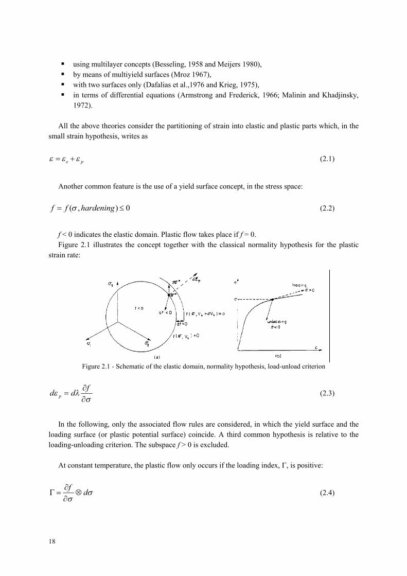
Figure 2.1 illustrates the concept together with the classical normality hypothesis for the plastic

strain rate:

Figure 2.1 - Schematic of the elastic domain, normality hypothesis, load-unload criterion

fdd p (2.3)

In the following, only the associated flow rules are considered, in which the yield surface and the

loading surface (or plastic potential surface) coincide. A third common hypothesis is relative to the

loading-unloading criterion. The subspace f > 0 is excluded.

At constant temperature, the plastic flow only occurs if the loading index, , is positive:

df

(2.4)

19

where the symbol indicates the contracted tensorial product. The opposite case implies elastic

unloading (see Figure 2.1, b).

All the models considered are a generalization in some way of the linear kinematic rule introduced

by Prager (1949), where the yield surface is described by

0)( kcf p (2.5)

Here the translation of the yield surface is denoted by the kinematic stress tensor (or back stress or

rest stress):

pcX ; pdcdX (2.6)

and the plastic multiplier d is determined through the consistency condition of time independent

plasticity: f = d f = 0.

It is simple to find at constant temperature, by using equations (2.3) and (2.4):

0

ffdcd

fdX

fd

fdf (2.7)

Taking account for the yield condition and the load-unload criterion leads to

ff

c

df

fHd )( (2.8)

Where:

H is the Heaviside function, H(u) = 0 if u < 0, H(u) = 1 if u > 0, and

the brackets are defined by < u > = u H(u).

Then the Equation (2.3) can be rewritten as follows:

ndnfHc

d p 1

(2.9)

where n is the unit outward normal to the yield surface

20

21

ff

f

n (2.10)

The hardening module is the constant c,

pp

p

dd

ddc

(2.11)

It has just described kinematic hardening, which represents rapid changes in the dislocation

structure. During each half-cycle (in tension-compression for example) dislocations are remobilized

when unloading and reverse loading take place. Then kinematic hardening gives a description of

monotonic rapid evolutions during each branch in a cyclic loading.

Independently of the kinematic effect, accumulation of dislocations can be represented by the

accumulated plastic strain. The corresponding strength modification can be introduced in the

modelling through a change in the width of the elastic domain: This change is given by the isotropic

internal stress in equation:

0 kRXJf (2.12)

where the kinematic and isotropic variables are X and R, respectively, which define position and

size of the yield surface; k is the initial size of the surface, with R(0) = 0.

The isotropic internal stress is directly related to the increase in the dislocation density, but may

also depend on the dislocation configuration, e.g. creation of dislocation cells, size and fineness of the

cells, etc.

2.4 Constitutive theories based on microscopic and/or crystallographic phenomenological

descriptions

Many different concepts are proposed in the literature for representing the thermo-mechanical

behaviour of material bodies: e.g. Jou et al. (1996), Maugin and Muschik (1994), Meixner and Reik

(1959), Muller and Ruggeri (1998), Truesdell and Noll (1965), and Ziegler (1977).

The development of the constitutive equations follows a thermo-mechanical framework, which was

established by Coleman and Gurtin (1967), Coleman and Noll (1963), and Truesdell and Noll (1965).

In this theory, the second law of thermodynamics is represented by the local form of the Clausius–

Duhem inequality and implies a constraint, which must be satisfied by the constitutive relations for

every admissible thermodynamic process (cf. the discussions in Jou et al. (1996) and Maugin and

Muschik (1994)). In contrast to this concept, Germain et al. (1983) introduces a pseudopotential of

dissipation and Green and Naghdi (1978) as well as Ziegler (1977) suggest a constitutive relation for

the rate of dissipation (cf. the remarks in Maugin and Muschik (1994)). In these frameworks, the

21

evolution equations of internal variables are often determined by using the postulate of maximum

dissipation (cf. Deseri and Mares, 2000; Miehe, 1998; Rajagopal and Srinivasa, 1998b), which can be

traced back in its thermo-mechanical formulation to Ziegler (1963) and Ziegler (1977). In plasticity

theory, a related concept was formulated by von Mises (1928) and Hill (1950).

In addition to the modelling of the mechanical behaviour, the representation of the thermo-

mechanical coupling phenomena is of special interest (Bodner and Lindenfeld, 1995; Chaboche,

1993b; Hakansson et al., 2005; Haupt et al., 1997; Helm, 1998; Jansohn, 1997; Kamlah and Haupt,

1998; Mollica et al., 2001; Tsakmakis, 1998): it is well known that metals show thermoelastic

coupling phenomena. Moreover, a part of the work required to produce plastic deformations is stored

as internal energy in the microstructure of the material. Since the basic results of Taylor and Quinney

(1934), this phenomenon has been investigated in detail: cf. Bever et al. (1973), Chrysochoos et al.

(1989), Helm (1998), Oliferuk et al. (1985), and Rosakis et al. (2000). In the first studies (cf. Taylor

and Quinney, 1934), a small amount of approximately 11% of the introduced cold work is stored in

the microstructure. In contrast to this, subsequent studies (e.g. Bever et al., 1973; Chrysochoos et al.,

1989; Helm, 1998; Oliferuk et al., 1985) led to the result that the stored energy depends on the

deformation history and that more than 11%, up to approximately 70%, of the cold work is stored in

the microstructure of the material.

A theory of viscoplasticity with adequate capabilities for modelling polycrystalline metals was

developed by Freed (1988). He developed a theory derived from physical and thermodynamical

considerations. The flow equation is of classical form. The dynamic recovery approach is shown to be

superior to the hardening function approach, for incorporating nonlinear strain hardening into the

material response through the evolutionary equation for back stress. A novel approach for introducing

isotropic strain hardening into the theory is presented, which results in a useful simplification. In

particular, the limiting stress for the kinematic saturation of state (not the drag stress) is the chosen

scalar-valued state variable. The resulting simplification is that there is no coupling between the two

state variables in the flow equation, and there is no coupling between dynamic and thermal recovery

terms in each evolutionary equation. This derived theory of viscoplasticity has the structure of a two-

surface plasticity theory when the response is plasticlike, and the structure of a Bailey-Orowan creep

theory when the response is creeplike. Its development was most strongly influenced by the

viscoplatic theories of Ponter and Leckie (1976) and Chaboche (1977).

Ponter and Leckie's theory is based on a Bailey-Orowan theory of creep (Bailey (1926) and

Orowan (1947)), Chaboche’s theory is based on a two-surface theory of plasticity (Dafalias and

Popov, 1975; Krieg, 1975). Others have also formulated viscoplastic theories based on those of Ponter

and Leckie (e.g., Robinson, 1978) and Chaboche (e.g., Walker (1981)).

Thermodynamics with internal variables offers a good framework to introduce constitutive

equations. It offers both a guideline and some constraints for the choice of thermodynamically

consistent evolution equations. A special form uses the notion of a standard generalized material,

where the complete thermo-elastic-inelastic behaviour is defined from the knowledge of two

potentials; the thermodynamic potential to describe the present state and the dissipative potential for

the irreversible evolutions.

Introducing mechanical constitutive models into a thermodynamic framework allows the partition

of the plastic work into the energy stored by the material and the one dissipated away as heat. The

constitutive equations are derived from the first and second laws of thermodynamics, the expression of

22

Helmholtz free energy, the additive decomposition of the total strain rate into elastic and visco-plastic,

the Clasius-Duhem inequality, the maximum dissipation principle, generalized normality, and the

thermo-mechanical heat equation. The visco-plastic yield criterion is of a von Mises type, but it needs

to be modified to account for high-strain rates and temperature dependency. This is done by replacing

the yield strength, the hardening function, and the viscous stress by the physically based flow stress

model. The irreversible thermodynamic process can be characterized by a time incremental approach

allowing for the equilibrium thermodynamic characterization. The irreversible thermodynamic is

compensated for by introducing internal state variables such that they are implicitly non-equilibrated

by a set of fictitious thermodynamic conjugate forces.

2.5 Constitutive rate-dependent theories

The inelastic response of materials is perhaps inevitably rate-dependent. When material rate-

dependence is accounted for, there is no loss for ellipticity in quasi-static problems and wave speed

remains real, as long as stress levels remain small compared to elastic stiffness. Even though the

phenomenology of localization can be the same for both rate-dependent and rate-independent material

behaviour, pathological mesh dependence does not occur in numerical solutions for rate-dependent

solids because boundary value problems remain well posed. The rate independent solid does emerge

as the appropriate limit.

One approach to remedying this situation is to explicitly introduce a length scale into the material

characterization by using a nonlocal constitutive relation. Material rate-dependence, no matter how

small, leads to well posed boundary value problems with unique solutions. This can be viewed in

terms of material rate-dependence implicitly introducing a length scale into the boundary value

problem formulation. Of course, in any particular circumstance, the question remains as to whether or

not this is the relevant length scale.

Since modern structures exhibit a strong rate-dependency especially at elevated temperatures, the

constitutive relations, which have been developed to describe the behaviour of different types of

metals, must be able to reproduce these facts. Processes related with high velocities therefore must be

described by a rate-dependent visco-plasticity whereas the same constitutive relations for vanishing

velocities must turn over to a rate-independent plasticity. Prior to establishing constitutive relations

that can fulfil these conditions, a proper physical interpretation of the phenomena observed during

inelastic deformation is needed.

This means that the different mechanisms that can explain the dissipation implied by internal

changes of the material are to be analyzed. It is known from appropriate microscopic investigations

that in a temperature, strain rate spectrum in general different regions can be observed reflecting

different mechanisms of inelastic deformation. Following some of them:

Athermal mechanisms characterized by a yield stress (e.g. face centred cubic metals) or

hardening stress (e.g., body centred cubic metals) relatively insensitive to the strain-rate;

Thermally activated dislocation motion. Characterized by a more markedly, temperature and

rate-sensitivity of the yield and hardening stresses.

23

Rice (1971) developed theoretical foundations of constitutive relations at finite strain for a class of

solids exhibiting inelasticity as a consequence of specific structural rearrangements, on the microscale

of constituent elements of material. Metals deforming plastically through dislocation motion are of this

class and form the primary application of the theory. The development is in terms of a general

internal-variable thermodynamic formalism for description of the microstructural rearrangements, and

it is shown how metal plasticity may be so characterized. The principal result is in the normality

structure, which is shown to arise in macroscopic constitutive laws, when each of the local

microstructural rearrangements proceeds at a rate governed by its associated thermodynamic force.

This provides a theoretical framework for time-dependent inelastic behavior in terms of a “flow

potential”, and reduces to statements on normality of strain increments to yield surfaces in the time-

independent case. Conventional characterizations of the stress-state dependence of metallic slip are

noted to be in accord with this concept of associated forces governing rates, so that the resulting

normality structure may be considered directly applicable to metal plasticity.

A rate-dependent constitutive theory was developed by Freed (1988): the Omega-form theory of

visco-plasticity, which is the normality structure of a potential function Omega. The advantage of this

approach is that the choice of two scalar-valued functions of state, completely defines a mathematical

structure for viscoplasticity. The disadvantage is that the theory may be too restrictive. This approach

results in a theory where inelastic strain-rate strongly influences the evolution of state, as is the case in

creep of metals. The ensuing discussion does not address physical justification for the existence of the

Omega function; rather, it concentrates on the mathematical consequences of such function. From this

theory a flow equation and an evolutionary equation for back stress were derived. The structure of this

evolutionary equation was alterated to introduce an evanescent strain-memory effect through the

addition of dynamic recovery term.

2.6 Constitutive modeling of cyclic plasticity and creep using an internal time concept

Typical constitutive relations for creep reported and used in literature include the modified strain

hardening rule developed by researchers at the Oak Ridge National Lab (Pugh et al., 1972, Corum et

al., 1974), dislocation models (Lagneborg, 1971, Gittus, 1976) based on metal physics, nonlinear

viscoelasticiy theory (Besseling, 1958); and the kinematic hardening model (Malinin and Khadjinsky,

1972) using an analogy to plasticity. However, efforts in material-constitutive-model development

reveal a trend toward unifying creep and plasticity. Some experimental results (Corum et al., 1974,

Jaske et al., 1975) were reported concerning the interaction between creep and plasticity. Further

details on the creep-plasticity interaction and unified models will be provided at the following

paragraph. Here, it is presented only a brief introduction, in which it is shown how these unifying

theories may be roughly divided into three categories of:

Potential theories

Microphenomenological theories

Nonlinear viscoplastic theories

Most studies employ these theories either individually or in combination. In the first category, one

may cite the theories using time-dipendent parameters (Kratochvil and Dillon, 1970), the concept of

kinematic hardening (Kujawski and Mroz, 1980), micromechanical considerations (Ponter and Leckie,

1976) and a combination of viscoplastic theory (Chaboche, 1977). The phenomenological theories

24

(Bodner and Partom, 1975; Hart, 1976, Hart et al., 1976; Miller, 1976a, 1976b; Krieg et al., 1978;

Robinson, 1978; Stouffer and Bodner, 1979) employ certain internal variables to reflect the

micromechanics of deformation, such as involving dislocations. Most of these theories assume that the

plastic strains are also time-dependent, as are creep strains, and that the creep surface will translate and

expand in the stress-space in a manner similar to that of isotropic and kinematic hardening used in

classical plasticity theory. The nonlinear viscoplasticity theories have the variations, in which: the

coefficients of the linear viscoelastic theory (Cernocky and Kremple, 1980) are expressed as a

function of stresses and strains, the inelastic strains are divided into viscous and viscoelastic

components (Findley and Lay, 1978), and the internal time is misured by the (total) strain history

(Valanis, 1971a, 1971b, 1980; Bazant and Bhat, 1976; Bazant, 1978, Wu and Yip, 1980, 1981;

Valanis and Fan, 1983). Of course, the fundamental aspects of inelastic deformation are also studied

(Rice, 1970, 1975; Hill and Rice, 1972) based on micromechanical considerations.

The intrinsic time theory, labelled “the endochronic theory” was presented by Valanis, (1971a,

1971b). This theory held out the prospect of explaining the experimental phenomena of cross-

hardening, cyclic hardening, and initial strain problems, the situations that classical plasticity theory

could not cope with. Bazant and Bhat (1976) also showed that the endochronic theory is effective in

dealing with problems of inelasticity and failure in concrete, and that Maxwell chain model can

describe the creep behaviour.

Valanis (1980) later presented a slightly modified intrinsic time model, wherein the internal time is

related to the inelastic strain. Valanis and Fan (1983) presented an incremental or differential form of

the integral relation of stress and strain (Valanis, 1980) for plasticity. This differential relation

(Valanis and Fan, 1983) is of a foundamentally different form as compared to that of the classical

plasticity theory and does not employ the notion of a yield surface nor the attendant concepts of

“elastic” and “plastic” processes. Based on such a differential relation, Valanis and Fan (1983)

developed an “initial strain” type iterative finite element approach. In this approach, the determination

of stress history (or the stress rate) from a given strain history (or the strain rate) is also highly iterative

in nature.

While using the concept of an intrinsic time, which depends on plastic strains, and the integral

relations of stress and strain (Valanis, 1980), Watanabe and Atluri (1986) rederive a differential stress-

strain relation, such that:

The concept of a yield surface is retained

The definitions of “elastic” and “plastic” processes are analogous to those in classical

plasticity theories

It can be implemented in a computationally simple and efficient manner, via a “tanget-

stiffness” finite element method, and a “generalized-midpoint-radial-return” algorithm for

determining the stress history (or the stress rate) for a given strain history (or strain rate).

They also developed a simple theory for creep, using the concept of intrinsic time which is

measured by the inelastic strain as well as Newtonian time, both of which are irreversible.

2.7 Creep-plasticity interaction and unified models

The characterization of material behaviour at elevated temperatures plays an important role in the

design of structures such as in hot sections of modern jet engines and other power plants. The ASME

25

code (1974) defines accepttable levels of stress and strain in critical components of power plants

operating at elevated temperatures. The severe mechanical environment may often cause these

structures to operate near or beyond the yield limit of the material. Consequently, a unified theory of

creep and plasticity, applicable to cyclic loading, is often desiderable.

Inelastic deformation at elevated temperature is complicated, because creep-plasticity interaction,

recovery of hardening, and so on may take place.

For taking into account creep-plasticity interaction, it is usual to assume unified constitutive

models, in which creep strain and plastic strain are regarded as inelastic strain identically (eg, Miller,

1976; Robinson et al., 1976; Hart, 1976; Chaboche, 1977; Krieg, Swearengen, and Rhade, 1978;

Cernocky and Krempl, 1979, 1980; Walker, 1981). In such models, recovery of hardening due to

thermal softening is expressed by incorporating recovery terms in the evolution equations of hardening

variables on the basis of the idea of Bailey (1926) and Orowan (1946).

Unified constitutive models seems to be successful in describing inelastic deformation at elevated

temperature, as seen from many applications; for example, Inoue, Imatani and Sahashi (1985), Moreno

and Jordan (1986), Delobelle and Oytana (1987), Delobelle and Lexcellent (1988), Freed (1988),

Chaboche and Nouailhas (1989,b), Chan et al. (1988, 1989, 1990).

It is interesting to note that for modeling the viscoplastic behaviour of 316 stainless steel, Delobelle

and Oytana (1987) assumed macroplastic strain for active loading and microplastic strain for

unloading; the material hardens both isotropically and kinematically in the process of macroplastic

strain, whereas only kinematic hardening takes place for microplastic strain. This assumption is based

on their creep experiments at high and low stresses (Delobelle and Oytana, 1984).

The distinction between active loading and unloading was made also by Mroz and Trampezynsky

(1984) and Hayhurst (1988). Assuming the memory of maximal prestress by Mroz (1981, 1983) they

specified different evolution rules of back stress for active loading and unloading. The creep model

proposed was then applied to creep under cyclic loading.

Strain aging plays an important role in some metals such as 304 and 316 stainless steel. Delobelle

and Lexcellent (1988) developed a unified model in which the hardening due to strain aging is taken

into account, and applied it successfully to various inelastic deformations of 316 stainless steel in the

temperature range of 20-700°C.

To evaluate inelastic constitutive models relevant to the material response under plasticity-creep

interaction, bench-mark studies were conducted by the Subcommittee on Inelastic Analysis and Life

Prediction of High Temperature Materials, JSMS (Inoue et al, 1985b, 1989a,b); 10 types of

constitutive models were examined in comparison with experiments of 21/4Cr-1Mo steel at 600°C

under uniaxial and multiaxial loading conditions.

2.8 Similarities between models

Similarities between models proposed on the basis of completely different concepts have been

discussed in some works. It is important to acknowledge such similarities for understanding and

developing further models.

Such discussion was given first by Marquis (1979) and Chaboche and Rousselier (1983). They

showed equivalence between the nonlinear kinematic hardening rule of Armstrong and Frederick

(1966) and a simple two-surface model based on bounding and yield surfaces. It is noted that these

models were proposed independently; ie, the Armstrong-Frederick rule was formulated by

incorporating a memory erasure (ie, dynamic recovery) term into the linear kinematic hardening rule,

while two-surface models were developed by Dafalias and Popov (1975, 1976) and Krieg (1975) on

26

the underlying idea of the multisurface model of Mroz (1967). Further detailed discussion concerning

the multisurface model, two-surface models, and the nonlinear kinematic hardening rule was given by

Chaboche (1986).

Watanabe and Atluri (1986a,b), on the other hand, showed that the endochronic theory of Valanis

(1980), with the kernel expressed in terms of the Dirac delta function and a series of exponential

functions, results in the generalized nonlinear kinematic hardening rule (Chaboche and Rousselier,

1983), in which back stress consists of components obeying the rule of Armstrong and Frederick

(1966). The endochronic theory of Valanis (1971, 1980) is one of the hereditary theories, and the

nonlinear kinematic hardening rule belongs to internal variable theories. Watanabe and Atluri (1986a,

b), furthermore, discussed that an appropriate choice of the kernel may result in the multisurface

model of Mroz (1967) and the two-surface models of Dafalias and Popov (1975, 1976) and Krieg

(1975).

Ohno and Wang (1990a) transformed the generalized nonlinear kinematic hardening rule by

Chaboche and Rousselier (1983) into a multisurface form. It was thus shown that the multisurfaces

generated by the transformation are nonintersecting, and that the translation of each surface relative to

the surrounding surface obeys the rule of Mroz (1967). Then applying the transformation to time

recovery terms and temperature-rate terms, they derived multisurface forms of these terms.

Chaboche (1989a) pointed out that the constitutive model developed at ONERA has similarities

with other models such as the time-independent model by Ohno-Kachi (1986), the unified viscoplastic

models by Walker (1981) and Krempl et al. (1986), and the differential form derived by Watanabe and

Atluri (1986a, b) for the endochronic theory of Valanis (1980).

Although recent advance has been achieved in elaboration or improvement of existing models,

some new concepts were presented, together with similarities with other models.

As seen in this review, the modeling has been developed so significantly. Thus highly sophisticated

constitutive models which describe most of the phenomena needed for engineering applications are

now available. However, further studies are still necessary for modeling complex phenomena such as

non-proportional hardening and flow behaviour, ratcheting behaviour, thermomechanical behaviour

and so on. Especially when they are coupled with strain aging, they cannot be predicted properly

without elaboration and improvement of models.

2.9 Chaboche EVP model

The current state of art of the modeling is mostly based on the concepts and models mentioned

above.

In the present work, the Chaboche elasto-visco-plastic theory has been chosen to develop a material

model able to describe the real behaviour for high temperature components subjected to cyclic loads.

Chaboche EVP model allows to simulate, with reasonable accuracy, all the essential mechanical

behaviour of Nickel base superalloy in the temperature range in which components, as gas turbine

blades, normally work.

This material model is a generalized implementation of elastic, elastic-plastic or visco-plastic, and

multi potential constitutive equations. The model is constructed entirely using object “bricks”. For the

moment, the model will be constructed using an elasticity object, a number of “potentials" and

27

interactions between the potentials. Potentials represent inelastic dissipations, which describe the

evolution of independent inelastic deformation mechanisms.

Hardening mechanisms are modelled with objects within the individual potentials (type of

hardening depending on the type of potential) and are thus not yet specified. This behaviour is

essentially a manager of sub-model objects, and will be discussed in general terms about the

permissible variables.

The model’s internal variables are determined by the sub-objects, which have been selected by the

user. The general storage form includes variables, which are “global" to the material laws, and

therefore form relations with the imposed (observable) variables or apply to all the potentials. Each

potential may additionally contain “parameter" variables, which do not have associated forces, and

“hardening" variables, which do have associated forces. The distinction concerns the form of

interaction, which is possible.

2.9.1 Costitutive Laws

In this model, total strain to can be divided into the following terms:

plthelto (2.13)

In which:

el = elastic strain

th = thermal strain

pl = plastic or inelastic strain

In the same way, total strain rate can be divided into the following terms:

plthelto (2.14)

Where overwritten symbols represent time derivatives of the terms.

In the proposed EVP Chaboche model, the plastic strain rate is pl expressed as:

npl (2.15)

With the Norton law:

n

K

f (2.16)

28

being:

XJ

Xn

2

''

2

3(2.17)

Where f is the effective tension von Mises Criterion:

RXJf 2 (2.18)

In the overwritten equations, the apexes quantities indicate the deviatoric component of tension:

ijkkijij 3

1' (2.19)

According to the following definitions:

Stress first invariant (or linear invariant):

332211 kk (2.20)

Kronecker’s delta or unit tensor:

ji

jiij

,0

,1 (2.21)

Stress second invariant (or Von Mises Equivalent Stress)

ijijijij XXXJ 2

32 (2.22)

The stress tensor X represents kinematic hardening, and corresponds to the stress variation in the

elastic dominion. X is called back stress too.

In Chaboche elasto-visco-plastic model kinematic hardening rule is non linear and is expressed

through the Armstrong-Frederick non-linear law:

CX3

2 (2.23)

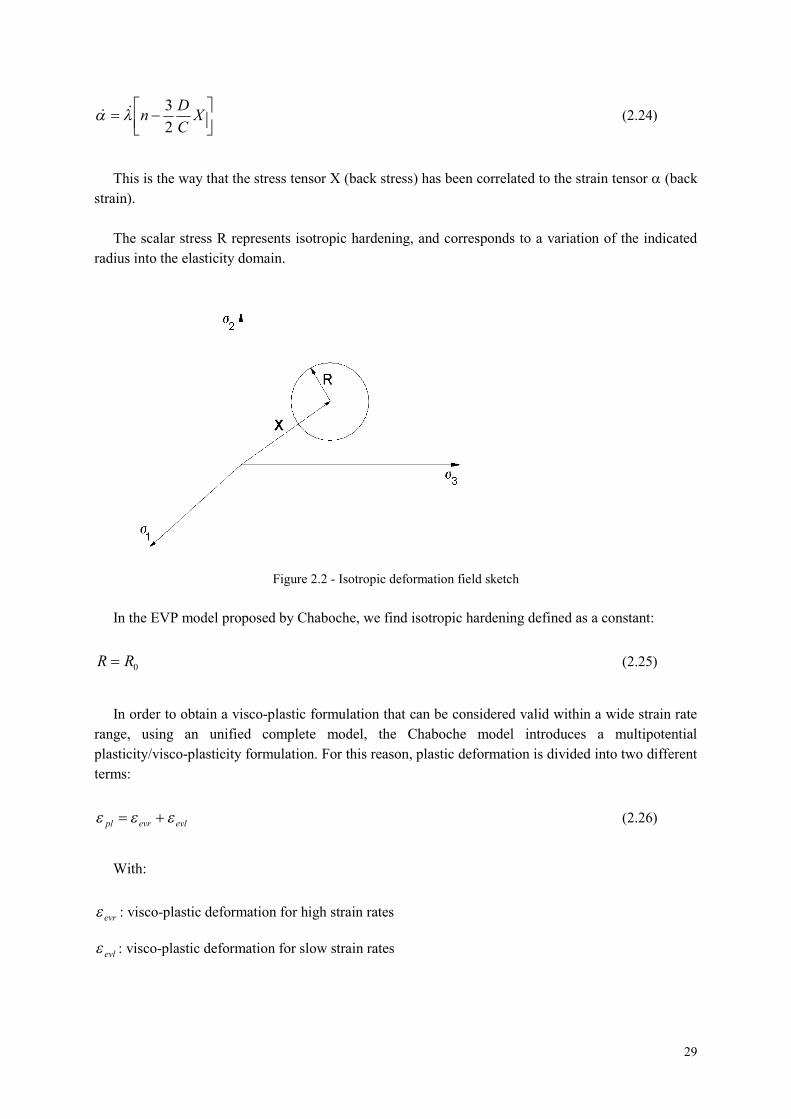
29

X

C

Dn

2

3 (2.24)

This is the way that the stress tensor X (back stress) has been correlated to the strain tensor (back

strain).

The scalar stress R represents isotropic hardening, and corresponds to a variation of the indicated

radius into the elasticity domain.

Figure 2.2 - Isotropic deformation field sketch

In the EVP model proposed by Chaboche, we find isotropic hardening defined as a constant:

0RR (2.25)

In order to obtain a visco-plastic formulation that can be considered valid within a wide strain rate

range, using an unified complete model, the Chaboche model introduces a multipotential

plasticity/visco-plasticity formulation. For this reason, plastic deformation is divided into two different

terms:

evlevrpl (2.26)

With:

evr : visco-plastic deformation for high strain rates

evl : visco-plastic deformation for slow strain rates

30

Both strain potentials have got visco-plastic features, their strain functions depend directly from

time. The first potential has got a yielding point and an hardening rule. The second one, instead, give

us a creep evolution mechanism including neither hardening nor yielding.

In this way, the first potential will give:

rrevr n (2.27)

With:

rn

r

rr

K

f (2.28)

XJ

Xnr

2

''

2

3(2.29)

02 RXJfr (2.30)

In this way we will have:

XJ

X

K

RXJrn

r

evr

2

''02

2

3 (2.31)

The first potential (usable for high strain rates) will result dependent from these parameters:

nr, Kr, that define Norton’s Law

C, D, that define kinematic Hardening

R0 (yielding point), that defines isotropic hardening

The second potential will give:

llevl n (2.32)

With:

ln

l

ll

K

f (2.33)

31

2

'

2

3

Jnl (2.34)

2Jfl (2.35)

In this way, user will obtain:

2

'2

2

3

JK

Jln

l

evl (2.36)

The second potential (vailid for slow strain rates) will be defined by the two following parameters:

nl, Kl, that define the well known Norton’s Law.

32

3 User-defined Material Models - Methods of Implementation in FEM software

3.1 Introduction

Plastic/Visco-plastic deformation in metals is a very complex phenomenon originating from highly

nonlinear dynamical processes associated with microscopic defects, such as dislocations that tend to

self-organize in the form of patterns, resulting into a heterogeneous field of deformation at the micro-

scale although the overall macroscopic field is thought to be homogeneous.

Although there has been a tremendous effort to understand work hardening/strain softening and

associated material instability phenomena, this research area is still in a parlous state, and rife with

controversy. This is due to the difficulty of carrying out truly definitive experiments on critical aspects

of the evolution of the dislocation structure. However, more important have been the immense

theoretical difficulties of dealing with large numbers of dislocations and defects. Nevertheless, it is

well understood that plastic deformation and strengthening in metals can be related to a number of

heterogeneous patterns, such as dislocation cells, slip bands, micro-shear bands, persistent slip bands

and dislocation tangles, which are critical for material properties.

The understanding of high-strain-rate behaviour of metals is essential for the modelling and

analysis of numerous processes including high-speed machining, impact, penetration and shear

localization. Thus, a desirable goal in constitutive modelling is to develop models which are widely

applicable and capable of accounting for complex paths of deformation, temperature and strain rate

which represent the main requirements of large deformation problems. The intended applications of

the model as well as the availability and ease in obtaining experimental data specify the degree of

complexity of the constitutive model.

Moreover, the degree of success of the model mainly depends on the flexibility and simplicity of

determining material constants from a limited set of experimental data and capturing the important

aspects of static and/or dynamic behaviour, besides being mathematically and computationally

accurate.

In this chapter, it will be provided an overview of methods for implementing user-defined models

in FEM software (codes based on Finite Element Method).

Finally, it will be explained how the Chaboche EVP model, chosen for the present applications,

will be implemented in ANSYS code (FEM software used in this work) for executing nonlinear

analysis on structural components.

3.2 Methods for user-defined model implementation

Large-scale finite element numerical simulations provide a feasible approach for assessing the

performance of inelastic structural components operating under complex thermo-mechanical and

multiaxial loading conditions.

The global solutions for any discretized finite element model are typically achieved, from the

computational point of view, by an increment iterative procedure (e.g., Newton-Raphson technique).

33

The mathematical forms, accuracy and stability properties of a selected integration procedure will

directly affect the accuracy and efficiency of the overall finite element solution. The development of

stress integration algorithms with improved performance has received considerable attention in the

recent literature on computational plasticity and visco-plasticity. In this regard, due to their stability

and wide range of applicability, a number of well-established implicit schemes of time integration

have been attracted the attention of many authors for plasticity and visco-plasticity (Simo and Taylor,

1985, Simo, 1991; Simo and Miehe, 1992; Freed and Walker, 1993; Saleeb and Wilt, 1993; Bathe,

1996).

For solving initial-boundary value problems, the stress state must be calculated by integrating a

system of ordinary differential equations. In the framework of numerical methods like the finite

element method, the system of differential equations is numerically solved by an appropriate

integration scheme. In the framework of implicit finite element methods, the most popular strategy to

integrate plastic or visco-plastic models is the backward Euler scheme (see e.g. Hartmann et al., 1997;

Simo and Miehe, 1992; Simo and Hughes, 1998) as well as the exponential algorithm (see e.g. Miehe

and Stein, 1992; Simo, 1993), which was originally proposed in finite visco-plasticity by Weber and

Anand (1990).

The exponential algorithm has the advantage that the incompressibility of the inelastic

deformations is always fulfilled. In contrast to this, the backward Euler method does not preserve the

plastic incompressibility at finite step sizes. Consequently, the backward Euler scheme leads to

incommensurate errors if large step sizes are applied (see e.g. the numerical studies in Tsakmakis and

Willuweit (2003)). In Simo et al. (1985), Simo and Miehe (1992) and also in Lu¨hrs et al. (1997) the

error is eliminated due to an additional assumption, which leads to a cubic equation for a scalar-valued

variable.

A number of material-related factors can cause structure's stiffness to change during the course of

an analysis. Nonlinear stress-strain relationships of plastic, multilinear elastic, and hyperelastic

materials will cause a structure's stiffness to change at different load levels (and, typically, at different

temperatures). Creep, visco-plasticity, and viscoelasticity will give rise to nonlinearities that can be

time-, rate-, temperature-, and stress-related. Swelling will induce strains that can be a function of

temperature, time, neutron flux level (or some analogous quantity), and stress.

Any of these kinds of material properties can be incorporated into an ANSYS analysis using

appropriate element types or a special material model. Nonlinear constitutive models are not

applicable for the ANSYS Professional program.

3.2.1 Object oriented software, modules and classes

Method of modelling chosen in the actual work is based on aided object oriented programming and

design. By the use of advanced programming languages (C++, Fortran 90) and programming,

customizing and interfacing of API (Application Programming Interfaces) by software dedicate to

material-analysis, it is possible to create and manage material library of assembling objects and

classes.

34

The most advanced software, nowadays, are programmed and compiled using tools that can be

assimilated with boxes. In each box, user can find useful tools (in this case constitutive equations of

material behaviours). These boxes, to be versatile and usable for many purposes, have to be provided

with user programmable features that, on one side, have to be able to interface the program with the

outer world, while on the other one should be able to provide user-friendly commands and scheme to

allow user building his functions.

In particular, user programmable features allow creating subroutines that interact with FEM solver. In

this work, USERMAT is the subroutine containing material constitutive laws. Solver recalls it, at each

integration point and for each equilibrium iteration. Inputs for each cycle are states variables, stresses,

strains, strain increments and time variable. Output of each cycle is the Jacobian Material Matrix

(stress, strain) at the end of each time increment.

This is allowed by using modular software for creating objects and classes to associate each one.

This is almost the same structure for all modular software that are used for material model simulations.

3.2.2 Z-Mat

Z-Mat is the software used in the present work to develop a user-defined material model to be

implemented in a FEM code, for performing elasto-visco-plastic analisys on structural componets.

The Z-Mat product is mainly a library of material behaviour routines (constitutive equations),

which can be interfaced with FEM software, and its supporting utilities. In contrast with other FEM

software products however, Z-Mat is built on C++ with a strong object-oriented design, and many

utility programming classes for advanced tensorial mathematics. Such advanced program design

techniques have enabled the software to be enormously extensible, on many different levels of

sophistication. In developing extensions to Z-Mat, a user can make new behaviours using the many

abstract “material model building bricks" to create a modular, flexible model based on fundamentals.

For final use, it then lets the different implemented “bricks" define the specifics. That is to say, the

user always chooses the final model form (e.g specific evolution or state equations) in the input file,

after development is finished. In that way, each model is really a “model class" or framework within

which a user has a high degree of flexibility. One can also add to the “types" available for these

building bricks. This allows extending the capabilities of every model using that particular abstract "

type”.

The program itself is organized in different modules. In Figure 3.1, it is introduced a schematic

view of Z-Mat modules:

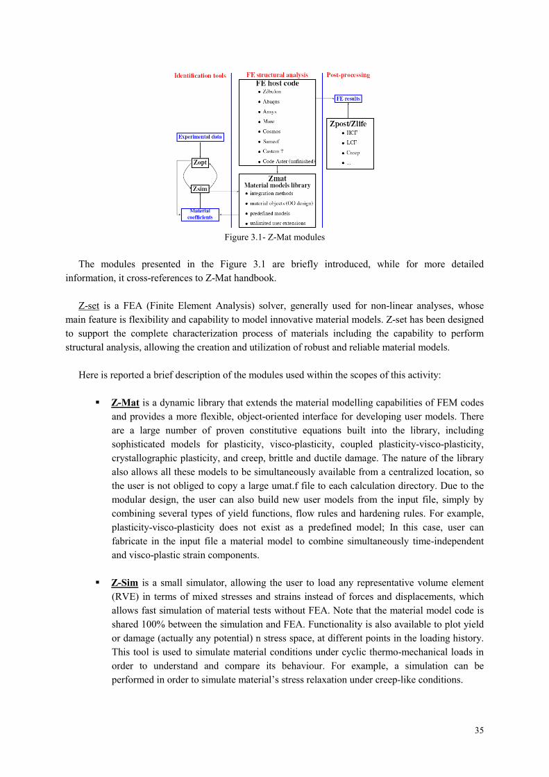
35

Figure 3.1- Z-Mat modules

The modules presented in the Figure 3.1 are briefly introduced, while for more detailed

information, it cross-references to Z-Mat handbook.

Z-set is a FEA (Finite Element Analysis) solver, generally used for non-linear analyses, whose

main feature is flexibility and capability to model innovative material models. Z-set has been designed

to support the complete characterization process of materials including the capability to perform

structural analysis, allowing the creation and utilization of robust and reliable material models.

Here is reported a brief description of the modules used within the scopes of this activity:

Z-Mat is a dynamic library that extends the material modelling capabilities of FEM codes

and provides a more flexible, object-oriented interface for developing user models. There

are a large number of proven constitutive equations built into the library, including

sophisticated models for plasticity, visco-plasticity, coupled plasticity-visco-plasticity,

crystallographic plasticity, and creep, brittle and ductile damage. The nature of the library

also allows all these models to be simultaneously available from a centralized location, so

the user is not obliged to copy a large umat.f file to each calculation directory. Due to the

modular design, the user can also build new user models from the input file, simply by

combining several types of yield functions, flow rules and hardening rules. For example,

plasticity-visco-plasticity does not exist as a predefined model; In this case, user can

fabricate in the input file a material model to combine simultaneously time-independent

and visco-plastic strain components.

Z-Sim is a small simulator, allowing the user to load any representative volume element

(RVE) in terms of mixed stresses and strains instead of forces and displacements, which

allows fast simulation of material tests without FEA. Note that the material model code is

shared 100% between the simulation and FEA. Functionality is also available to plot yield

or damage (actually any potential) n stress space, at different points in the loading history.

This tool is used to simulate material conditions under cyclic thermo-mechanical loads in

order to understand and compare its behaviour. For example, a simulation can be

performed in order to simulate material’s stress relaxation under creep-like conditions.

36

Z-Optim Optimization including several classical methods such as SQP, simplex or

Levenberg-Marquardt, and genetic algorithms. In connection with Z-Sim this is a powerful

tool for the identification of material parameters, while keeping exactly the same user

interface as Z-Mat and Z-Sim. The optimal parameters can be determined through a

process of least square minimization process using a set of experimental curves for

reference and the simulated ones.

Z-Post is a module to manage FEM results data post-processing execution and operations.

It can be used to evaluate damage from fatigue and creep with the aim of calculating life of

a structural component. It has interfaces and subroutines to be able to read results file from

many FEM software.

Z-Ansys is a bunch of tools that allow executing advanced and complex FE analyses,

oriented to manage much material behaviour, utilizing ANSYS. This module uses a

dynamic library of materials in order to extend ANSYS capabilities to model different

material behaviours. It has a simple and powerful interface to develop new material

models. It is linked directly to Z-Mat, Z-Sim and Z-Opt.

In the following periods, there will be described briefly how constitutive equations can be arranged

in order to obtain the material card useful for an elasto-visco-plastic analysis.

In a Finite Element code, constitutive equations are used at each integration point to simulate

material behaviour. Z-Mat adds capability by providing advanced constitutive equations based on the

rigorous thermodynamic state variable formulation.

The primary numerical task for material simulation code for FEA calculations is to provide the

value of the stress tensor and the state variables at the end of a loading increment, knowing the values

at the beginning of the increment and a trial strain increment. More precisely, we can define an

“object” BEHAVIOR as the collection of:

Primal prescribed variable (e.g. strain) and dual (associated) variable (e.g. stress).

Set of state dependent variables V.

Set of auxiliary variables, A, not necessary for the computation, but used in the post-

processing.

External parameters, P, prescribed by the user and acting like an external load (e.g.

temperature in a mechanical uncoupled calculation).

Material parameters, M, to be identified for each material.

The constitutive equations are normally expressed as a first order ordinary differential system

(ODE), the derivative of the state variables being defined as functions of the prescribed primal

variable, of A, P and M. The integration of this system can be made by explicit and implicit methods.

Both techniques are included in Z-Mat as follows:

Runge-Kutta method with automatic time stepping.Modified midpoint (q-method), solved with a Newton algorithm.

37

The explicit integration is easier to implement, and therefore is used for fast prototyping. Implicit

integration however demands the definition of the local Jacobian matrix defining the behaviour, which

is a more complex affair, but the method is more robust for large time steps, as it provides the

information needed to compute the global consistent tangent matrix, and therefore permit quadratic

global convergence.

Z-Mat treats all model formulations in the most general sense, employing object-oriented design to

achieve a high level of flexibility. With this approach, the models are described in terms of material

building “bricks,” such as yield criterion, isotropic or kinematic hardening evolution, or visco-plastic

flow. A model is much more powerful with this approach because all the different “brick” types can be

combined by the user to effectively make new models at run-time. In fact, even the coefficients are

generalized (abstracted), allowing constant values, tabular values, or c-type syntax functions.

There are two ways of using Z-Mat:

User-modeDeveloper-mode

As many constitutive equations are already implemented in Z-Mat, most users can simply make use

of those in their calculations. A small change in the ANSYS input file is necessary to access the Z-Mat

library, and an external material definition file must be created.

The input file modifications must give the material name, which will become the name of an

external material definition file to control Z-Mat. The number of state variables is also required. Z-Mat

does not use any information regarding coefficients or material parameters from the ANSYS input.

Any number of Z-mat materials is accepted in the same run.

3.2.2.1 Z-Mat Material Behaviours

Material behaviours are a set of constitutive equations that are built from fundamental “building

bricks" of sub-models. There is widespread re-use of all these “bricks" between different behaviour

models.

The most important concept is the notion of a class of permissible options, of which the user will

choose one or more objects from that class in the material definition.

A class is an abstract notion of basic functionality. An example is the ELASTICITY class that

handles the calculation of stress from a strain, usually employing a fourth order tensor of various

modulus coefficients. Because of this very general function, many behaviour models allow for an

ELASTICITY instance.

38

Figure 3.2- Z-Mat Objects and Classes

In turn, the elasticity class has many possible types that one can select in an elasticity object

(isotropic, orthotropic, etc).

FEM software actually do not include in their libraries, the elasto-visco-platic material model, since

its complexity and high technology content, together with the limited computational capacity of most

of common personal computers, did not permit its implementation.

Figure 3.3- Z-Mat Objects + Classes = Constitutive laws

This is the reason why to implement such model, is necessary to use external software like Z-mat.

In Figure 3.3, it is shown a typical assembly for elasto-visco-plastic material behaviour. By the

coupling of classes and objects, the constitutive equations that describe material behaviour have been

selected. This modelling method has allowed implementing energy potentials, which, combined each

other, describe the mechanism of inelastic dissipation and deformation evolution. Complex and

superimposing hardening mechanisms are modeled by objects within individual potentials. In

particular, in the example in Figure 3.3, material model shows an isotropic elasticity and thermal

strain. The yield criterion chosen to describe plastic behaviour is the Von-Mises criterion and it has

been used the Norton equation to calculate the viscous stresses and to describe the visco-plasticity.

Finally to describe material hardening (and so the changes in yield surface) the superimposing of

isotropic constant and kinematic nonlinear behaviour has been selected.

3.2.2.2 Material Files

The material coefficients are defined in a separate file. The material file is a standard ASCII text

file of form similar to the main input file. Most instances where a material filename needs to be

39

specified allows an optional integer value for the instance of behaviour in that file, the default instance

being the first. So, when a material file is opened, the program will search for the nth occurrence of the

keyword ***behaviour, skipping all other data contained before. Frequently for example and

verification problems, the material file is given in the same physical file as the referring input file for

compactness and file management purposes.

Regardless of how or where the material file is located, the material file is a separate entity from

the other input commands, with an independent command hierarchy starting at the ***-level.

3.3 Z-Mat Chaboche model implementation

A particular form of the Chaboche model will be used, including thermal strain, non-linear

isotropic hardening, linear and non-linear kinematic hardening, and some coefficients that vary with

temperature. The behaviour model is only a framework for building up particular

hardening/criterion/flow/etc combinations. The basic form of the model has been stated at the previous

chapter, where the Chaboche constitutive laws for describing elesto-visco-plastic material behaviour

have been defined in detail.

The model supports any number of kinematic hardening variables, and all coefficients in the model

may be variable.

As shown previously, to start the material file, the ***behaviour keyword must be used to indicate

a generic behaviour object is to be created. All such objects will have a “class” keyword (here,

behaviour), followed by a particular type of that class. For this model, the type is gen_evp for

generalized elasto-visco-plastic. It should be noted that the asterisks in the Z-mat file indicate not only

keywords, but a hierarchy of sub-commands. Thus all keywords of **-level are sub-commands of the

behaviour, and the next ***-level command (here ***return) terminates the behaviour read. For this

model, the elasticity matrix, thermal strain, and potential keywords are used.

The potential object is the most interesting one here, as it defines all the plasticity characteristics.

The potential model chosen is again named gen_evp (but could be one of many others), and the

characters following are an optional name for the potential. Output variables and coupling use this

user-determined name.

The following is an example of Chaboche EVP model. It has been created by joining each

applicable class with corresponding subclasses and tuning opportunely their instances and values.

40

***behavior gen_evp auto_step**elasticity isotropic

young temperature215000.0 20.

…………………….poisson 0.3

**thermal_strain isotropicalpha temperature0.12500000E-04 0.

.................................**potential gen_evp evr*criterion mises*flow norton

K temperature114.956 20.

n temperature12.496 20.*kinematic nonlinear

D temperature596.336 20.

C temperature187123.4 20.*isotropic constant

R0 temperature232.226 20.………………………**potential gen_evp evl*criterion mises*flow norton

K temperature3093.09 20.n temperature21. 20.*isotropic constantR0 0.

***return

Table 3.1 - Z-Mat elasto-visco-plastic material framework

The material file structure for the elasto-visco-plastic model consists of an elasticity object, an

optional thermal strain object, an optional arbitrary number of potentials (without restriction on types),

and a number of optional interaction objects:

A more detailed explanation of how it is possible to define a model of material behaviour through

the coupling of classes and objects, it is provided in Z-Mat handbook.

The compatibility of objects with the other objects, and with the integration method will be

investigated during the running of the problem. Because of the dynamic nature of these models

however, it is often difficult to make any verification as to the physical meaning of a particular model

combination. It is therefore strongly advised to observe the material behaviour on a single element.

This allows experimentation of the integration method and selection of the output variables without

performing costly full-scale calculations.

Multi-potential models are primarily used for cases of time independent plasticity in combination

with visco-plastic deformation, or to assemble multiple crystalline deformation systems.

By default, there is no thermal strain, no inelastic deformation or any interactions. The optional

names (name) given after each potential type are used as a means to specify individual potentials (for

interactions), and in construction of the output variable names.

Normally, it is advised to use ep for a plastic potential name, and ev for a visco-plastic one.

41

4 Material Characterization

4.1 Introduction

The material behaviour characterization may be definied as: determining the material model

response that better reproduces the observed experimental behaviour by using a design optimization

framework.

In the present chapter it will be described the methodology of material characterization by:

designing the experimental tests necessary to describe the aspects of material behavior that

have to be investigated

choosing the constitutive laws that better reproduce material behavior

describing the iterative procedure for determining the coefficients of material model

describing the procedure of model validation by means the comparison between

experimental data and simulated ones.

The chapter is separated in five sections: theory, numerical methods, analysis of experimental data,

limits of automatic procedure, design of experiments.

In the first section, it will be provided a theoretical description of material characterization tests.

They can be summarized in tensile, fatigue and creep tests. It will be described the way in which the

tests have to be performed, the type of specimen, the test machine and the main coefficients obtaining

by them. Besides, it will be provided also a description of Chaboche elasto-visco-plastic material

model chosen for the present applications, the constitutive laws and the meaning of each model

parameter.

In the section of numerical methods, it will be described the methodology of material

characterization: an iterative procedure of simulation of experimental tests and optimization of

constitutive model coefficients through the comparison with the experimental data (by minimizing the

least-square distance between experimental data and simulated curves). Besides, it will be described

the procedure of model validation too.

In the third section, it will be analysed the experimental data. In particular, the described procedure

will be applied for characterizing a Nickel base super-alloy, extensively used in high temperature

components of jet engines and gas turbines for power generation.

In the fourth section, it will be described how the quality of performed experiments influences the

material characterization process and the limits of an automatic characterization procedure will be

highlighted.

The last section will provid guidelines for designing experimental tests able to identify optimized

parameters set of material model.

42

4.2 Material Characterization – Theory

4.2.1 Experimental tests

Material characterization methodology is based on observed experimental results. Following it will

be presented some basic elements on the types of tests, the machines and the modern measurement

techniques likely to be used. Progress in electronics, automatic controls, digital measurements and in

microprocessors has resulted in a radical transformation of the laboratories engaged in characterization

of materials. One no longer has to be content with approximate measurements of a few quantities;

since now it is possible to measure the evolution of any mathematically well defined variable

precisely. The identification of complex models has thus become possible, but it requires numerical

methods for the identification of nonlinear processes, which still belong to the domain of ‘heuristic’

techniques (Lemaitre and Chaboche, 1990)

Experimental tests represent the better way to obtain useful data and information on material

characteristics. In fact, materials behaviour of components in service is strongly affected by their

chemical mechanical and structural characteristics. This is the reason why it is important to know and

well evaluate material properties.

The first step is the definition of the matrix of necessary experimental tests to the characterization

of material behavior.

The present study has in particular dealt with the research of correlation between results of

mechanical tests and fatigue, creep, yield stress and rupture sensitivity.

The complete tests matrix has to be designed in order to provide a sufficient statistical base to

calculate minimum and average material curves and to obtain all the necessary experimental data for

determining the material coefficients required by Chaboche elato-visco-plastic model.

Tensile tests at various temperatures are used to determine base material mechanical properties

such as Young’s Modulus, yield strength, Poisson’s ratio, etc.

Tensile tests at various temperatures and different strain rates are performed for determining the

viscous effects and the viscosity parameters k and n (Norton’s flow parameters in elasto-visco-plastic

Chaboche model)

LCF and HCF tests are performed in order to characterize material behaviour subjected to

controlled-load cycle at various loading-rates. Some tests are performed in order to determine material

hardening behaviour. Others have the objective to evaluate material stabilization laws.

High temperature creep tests are performed in order to evaluate creep behaviour of the superalloy.

With more details on this subject, stress relaxation time is extracted from this type of test. Besides,

creep strain is one of the most important data that it is possible to obtain from these tests.

4.2.2 Tensile Test

Tests are performed according to the ASTM standards. A tensile test measures the resistance of a

material to a static or slowly applied force. A machined specimen is placed in the testing machine and

load is applied. A strain gage or extensometer is used to measure elongation. The stress obtained at the

highest applied force is the tensile strength. The yield strength is the stress at which a prescribed

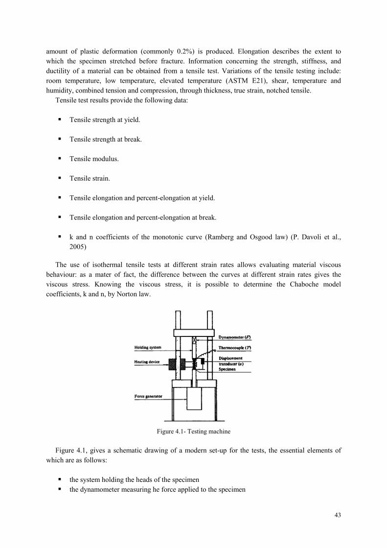
43

amount of plastic deformation (commonly 0.2%) is produced. Elongation describes the extent to

which the specimen stretched before fracture. Information concerning the strength, stiffness, and

ductility of a material can be obtained from a tensile test. Variations of the tensile testing include:

room temperature, low temperature, elevated temperature (ASTM E21), shear, temperature and

humidity, combined tension and compression, through thickness, true strain, notched tensile.

Tensile test results provide the following data:

Tensile strength at yield.

Tensile strength at break.

Tensile modulus.

Tensile strain.

Tensile elongation and percent-elongation at yield.

Tensile elongation and percent-elongation at break.

k and n coefficients of the monotonic curve (Ramberg and Osgood law) (P. Davoli et al.,

2005)

The use of isothermal tensile tests at different strain rates allows evaluating material viscous

behaviour: as a mater of fact, the difference between the curves at different strain rates gives the

viscous stress. Knowing the viscous stress, it is possible to determine the Chaboche model

coefficients, k and n, by Norton law.

Figure 4.1- Testing machine

Figure 4.1, gives a schematic drawing of a modern set-up for the tests, the essential elements of

which are as follows:

the system holding the heads of the specimen

the dynamometer measuring he force applied to the specimen

44

the transducer measuring the variation of length of the specimen

the frame of machine, which should be as stiff as possible

the heating device

the device for applying the forces

During the test, the load is applied in specimen axis direction with constant and prefixed increasing

rate (strain-controlled test).

The specimen presents an utilizable length at constant section joined with the extremities heads.

Following (Figure 4.2) a typical specimen geometry:

Figure 4.2- Specimen for tension test - Definitions

In Figure 4.2, on the left a specimen with circular section, on the right a specimen with rectangular

section.

The useful part of the specimen is constituted by an utilizable length L0 (Figure 4.3) and two

lengths (C) that allow to obtain a uniform stress field before of L0 beginning.

Figure 4.3- Specimen for tension test

In order to obtain comparable results, the specimens have to respect the following dimensions:

00 SkL (4.1)

Where S0 is the section and k is a coefficient that may be obtained by ASTM standards, in

particular in case of specimens with circular section, L0 is assumed:

00 10 dL or 00 5 dL (4.2)

Where d0 is the diameter of the section.

The Figure 4.4 shows the curve - in which: R is the maximum stress, sis the yield stress. The

elastic, plastic and striction fields are the indicated areas.

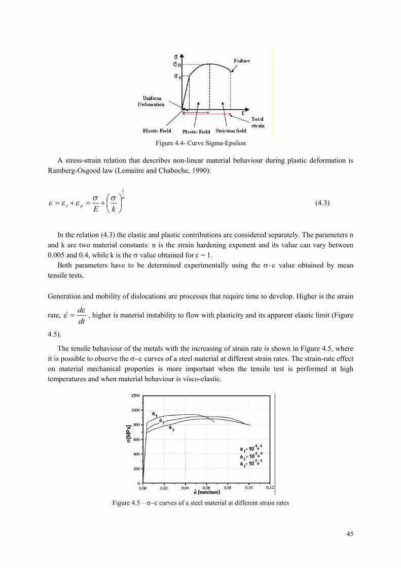
45

Figure 4.4- Curve Sigma-Epsilon

A stress-strain relation that describes non-linear material behaviour during plastic deformation is

Ramberg-Osgood law (Lemaitre and Chaboche, 1990):

n

pekE

1

(4.3)

In the relation (4.3) the elastic and plastic contributions are considered separately. The parameters n

and k are two material constants: n is the strain hardening exponent and its value can vary between

0.005 and 0.4, while k is the value obtained for = 1.

Both parameters have to be determined experimentally using the value obtained by mean

tensile tests.

Generation and mobility of dislocations are processes that require time to develop. Higher is the strain

rate,dt

d , higher is material instability to flow with plasticity and its apparent elastic limit (Figure

4.5).

The tensile behaviour of the metals with the increasing of strain rate is shown in Figure 4.5, where

it is possible to observe the curves of a steel material at different strain rates. The strain-rate effect

on material mechanical properties is more important when the tensile test is performed at high

temperatures and when material behaviour is visco-elastic.

Figure 4.5 – curves of a steel material at different strain rates

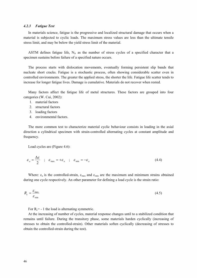
46

4.2.3 Fatigue Test

In materials science, fatigue is the progressive and localized structural damage that occurs when a

material is subjected to cyclic loads. The maximum stress values are less than the ultimate tensile

stress limit, and may be below the yield stress limit of the material.

ASTM defines fatigue life, Nf, as the number of stress cycles of a specified character that a

specimen sustains before failure of a specified nature occurs.

The process starts with dislocation movements, eventually forming persistent slip bands that

nucleate short cracks. Fatigue is a stochastic process, often showing considerable scatter even in

controlled environments. The greater the applied stress, the shorter the life. Fatigue life scatter tends to

increase for longer fatigue lives. Damage is cumulative. Materials do not recover when rested.

Many factors affect the fatigue life of metal structures. These factors are grouped into four

categories (W. Cui, 2002):

1. material factors

2. structural factors

3. loading factors

4. environmental factors.

The more common test to characterize material cyclic behaviour consists in loading in the axial

direction a cylindrical specimen with strain-controlled alternating cycles at constant amplitude and

frequency.

Load cycles are (Figure 4.6):

aaa

minmax ;;2

(4.4)

Where: a is the controlled-strain, max and min are the maximum and minimum strains obtained

during one cycle respectively. An other parameter for defining a load cycle is the strain ratio:

min

max

R (4.5)

For R= - 1 the load is alternating symmetric.

At the increasing of number of cycles, material response changes until to a stabilized condition that

remains until failure. During the transitory phase, some materials harden cyclically (increasing of

stresses to obtain the controlled-strain). Other materials soften cyclically (decreasing of stresses to

obtain the controlled-strain during the test).

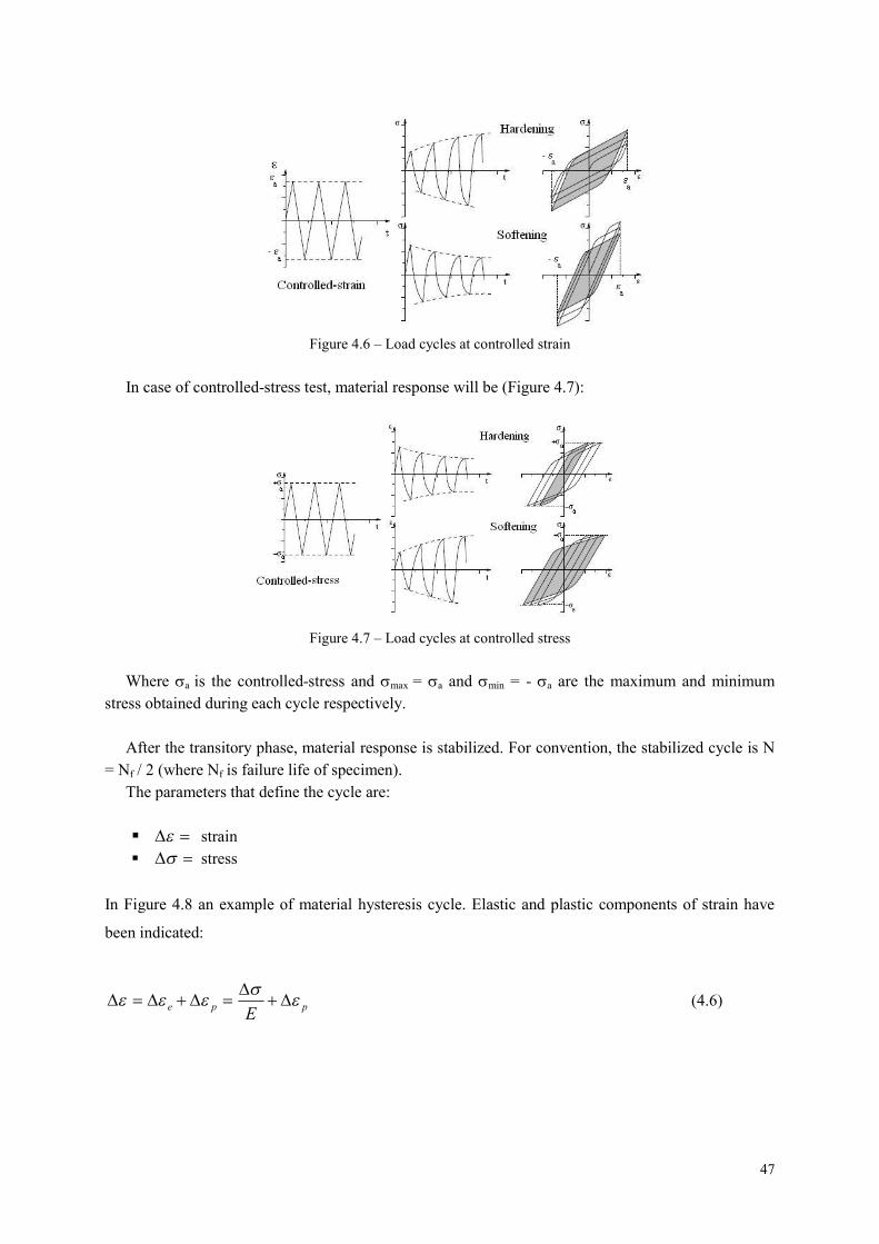
47

Figure 4.6 – Load cycles at controlled strain

In case of controlled-stress test, material response will be (Figure 4.7):

Figure 4.7 – Load cycles at controlled stress

Where a is the controlled-stress and max = a and min = - a are the maximum and minimum

stress obtained during each cycle respectively.

After the transitory phase, material response is stabilized. For convention, the stabilized cycle is N

= Nf / 2 (where Nf is failure life of specimen).

The parameters that define the cycle are:

strain

stress

In Figure 4.8 an example of material hysteresis cycle. Elastic and plastic components of strain have

been indicated:

ppeE

(4.6)

48

Figure 4.8 – Hysteresis cycle

The slope of the line is the Young Modulus E.

Repeating the cyclic tests with R = -1 at various controlled-strains (for example 0.1%, 0.2%, etc.),

different stabilized cycles will be obtained. Inserting in a same graph the stabilized cycles at different

controlled-strains and interpolating the vertex of these curves with Ramberg-Osgood equation, it is

obtained a typical material curve: the cyclic curve (Figure 4.9).

Figure 4.9 – Cyclic curve

Useful information about hardening or softening material behaviour are available by cyclic curve.

Figure 4.10 shows cyclic and monotonic curves of some materials:

49

Figure 4.10- Examples of cyclic and monotonic curves

By the observation of the relative position between the two curves, it is possible to obtain the

following information: cyclic hardening is verified when cyclic curve is upper monotonic one. On the

contrary, cyclic softening is verified when cyclic curve is lower monotonic one.

4.2.4 Creep Test

Creep is the tendency of a solid material to slowly move or deform permanently under the

influence of stresses. It occurs as a result of long term exposure to levels of stress that are below the

yield strength or ultimate strength of the material. Creep is more severe in materials that are subjected

to heat for long periods, and near the melting point. Besides, creep always increases with temperature.

The rate of this deformation is a function of the material properties, exposure time, exposure

temperature and the applied load (stress). Depending on the magnitude of the applied stress and its

duration, the deformation may become so large that a component can no longer perform its function,

for example creep of a turbine blade will cause the blade to contact the casing, resulting in the failure

of the blade.

Creep is usually of concern to engineers and metallurgists when evaluating components that

operate under high stresses or high temperatures. Creep is not necessarily a failure mode, but is instead

a deformation mechanism. Moderate creep in concrete is sometimes welcomed because it relieves

tensile stresses that otherwise may have led to cracking.

Unlike brittle fracture, creep deformation does not occur suddenly upon the application of stress.

Instead, strain accumulates as a result of long-term stress. In fact, creep deformation is "time-

dependent" deformation.

The temperature range in which creep deformation may occur differs in various materials.

Generally, the minimum temperature required for creep deformation to occur is 30% of the melting

point for metals and 40–50% of melting point for ceramics.

In modern jet engines, temperatures can reach up to 1400°C and initiate creep deformation in even

advanced-coated turbine blades. Hence, it is crucial for safety's sake to understand creep deformation

behaviour of materials.

Creep deformation goes through three stages:

50

Figure 4.11- Creep stages

By Figure 4.11 it may be observed that in the initial stage, or primary creep (I), the strain rate is

relatively high, but it slows with increasing strain. The strain rate eventually reaches a minimum and

becomes near constant. This is known as secondary (II) or steady state creep. This stage is the most

understood. The characterized "creep strain-rate" typically refers to the rate in this secondary stage.

Stress dependence of this rate depends on the creep mechanism. In tertiary creep (III), the strain rate

exponentially increases with strain.

The material behaviour under high temperatures and mechanical loads is described through creep

tests: a cylindrical specimen is subjected to a constant state of stress at a fixed temperature (Figure

4.12 – a). The strains are measured simultaneously by mean extensometers and the resulting variation

in strain as a function of time is determined (Figure 4.12 – b). This also characterizes the hardening

and the viscosity of material.

The strain variation, after the stress is removed (point B), corresponds to the recovery test. The

partial strain recovery is indicated in Figure 4.12 (b)

Figure 4.12- Creep test and subsequent recovery

The results can be used to estimate the deformation behaviour of components that are exposed to

long-term tensile stresses and high temperatures. These tests are quite often achieved for the

determination of creep limits in order to be able to perform structural dimensioning or guarantee that

the structure does not undergo any creep strain during operation.

It is also possible to perform a relaxation test during which strain is maintained constant (Figure

4.13 – a). By doing so, the stress is decreasing with time (Figure 4.13 – b). This gives information

concerning the behaviour of structural components and the evolution of stresses in case of imposed

strain. It is governed mainly by viscosity but also depends on the hardening induced by the initial load.

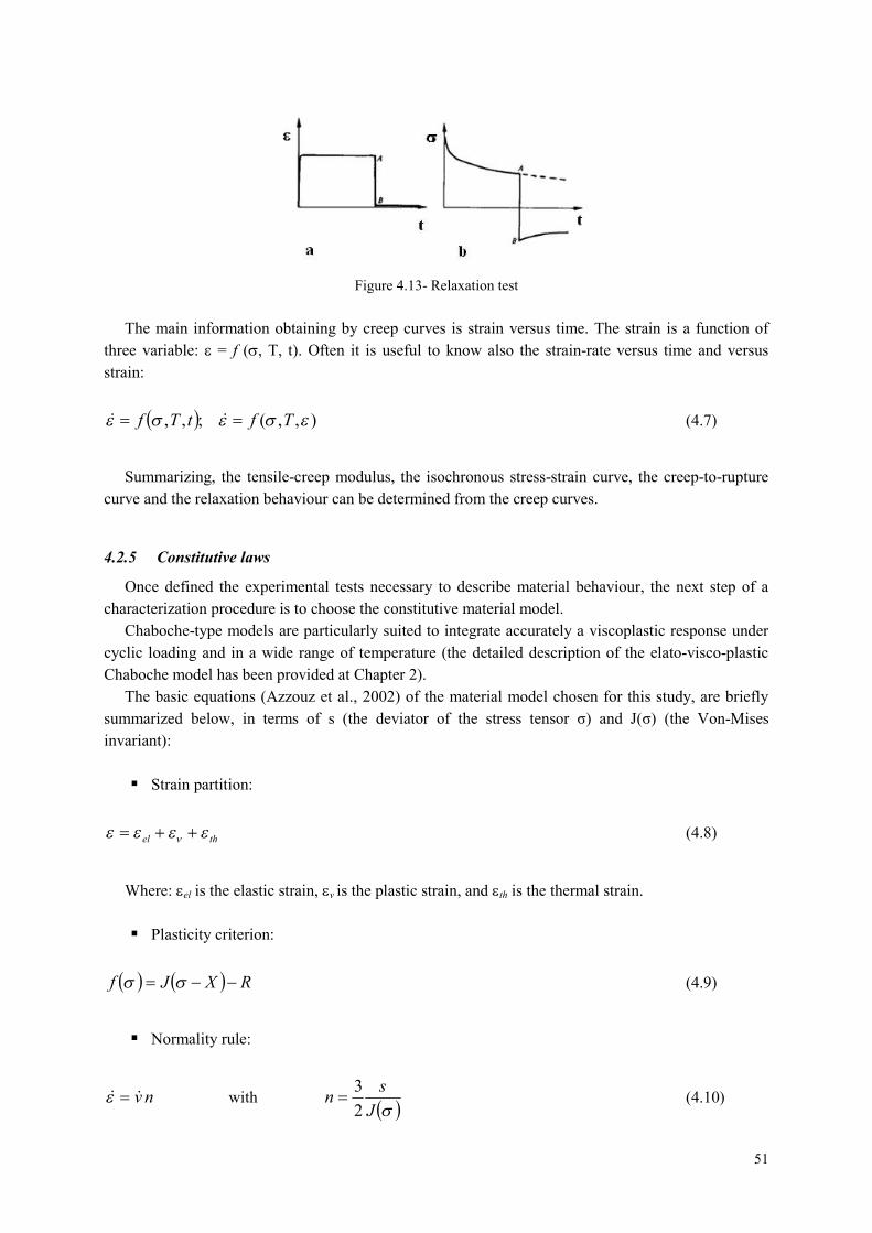
51

Figure 4.13- Relaxation test

The main information obtaining by creep curves is strain versus time. The strain is a function of

three variable: = f (, T, t). Often it is useful to know also the strain-rate versus time and versus

strain:

),,(;,, TftTf (4.7)

Summarizing, the tensile-creep modulus, the isochronous stress-strain curve, the creep-to-rupture

curve and the relaxation behaviour can be determined from the creep curves.

4.2.5 Constitutive laws

Once defined the experimental tests necessary to describe material behaviour, the next step of a

characterization procedure is to choose the constitutive material model.

Chaboche-type models are particularly suited to integrate accurately a viscoplastic response under

cyclic loading and in a wide range of temperature (the detailed description of the elato-visco-plastic

Chaboche model has been provided at Chapter 2).

The basic equations (Azzouz et al., 2002) of the material model chosen for this study, are briefly

summarized below, in terms of s (the deviator of the stress tensor σ) and J(σ) (the Von-Mises

invariant):

Strain partition:

thel (4.8)

Where: el is the elastic strain, v is the plastic strain, and th is the thermal strain.

Plasticity criterion:

RXJf (4.9)

Normality rule:

nv with J

sn

2

3 (4.10)

52

Norton flow:

n

k

fv

(4.11)

Nonlinear kinematic hardening:

CX3

2 with

X

C

Dnv (4.12)

Nonlinear isotropic hardening:

bveQRR 10 (4.13)

In order to take into account both the variation of the elastic domain dimension (isotropic model)

and its translation (kinematic non-linear model), it has been chosen the combined Chaboche model

(Delprete et al., 2007).

It allows describing the hardening evolution for metallic material under cyclic loads.

In the above equations:

the strain-rate dependence and the viscous effects are governed by a power law relation

(equation 4.11).

Cyclic hardening (evolution of the stress-strain loops from one cycle to the other) is

characterized by equation 4.13, where R is an exponential function of the cumulated plastic

strain v. In this expression, Q represents the amount of hardening between the first cycle and

the stabilized cycle, and b is the rate of saturation.

The equation 4.13 describes the variation of the elastic domain dimension.

Kinematic hardening (equation 4.12) is then introduced to characterize the reversible

hardening behaviour within each cycle. Integration of equation 4.12 also yields an exponential

form, with C/D the asymptotic value and D the rate of saturation (note that sharper transition

from elasticity to plasticity is obtained with higher values of D).

For strain-rate controlled uniaxial tests, the maximum stress level obtained on the stabilized cycle

can then be simply evaluated as:

D

CQRk n 0

1

(4.14)

The elastic behaviour is described on the base of the hypothesis of linear isotropic elasticity

(equation 4.8).

The hardening evolution in plastic field is described through two components:

53

Isotropic hardening, that models the evolution of the elastic domain dimension by recalculating

cycle by cycle the yielding stress;

Kinematic nonlinear hardening that models the translation of the elastic domain by calculating

the evolution of kinematic variable (back stress tensor).

The way to implement the elasto-visco-plastic Chaboche material model has been dealt at

paragraph 3.3 and its basic framework has been shown at Table 3.1.

The identification of material coefficients for such sophisticated model is a complex process that

necessitates efficient dedicated optimization tools. For the Chaboche model described above, there are

seven coefficients to identify for each temperature (in addition of thermo-elastic parameters): the

viscosity coefficients K and n, the isotropic hardening coefficients R0, Q and b, and the kinematic

hardening coefficients C and D.

4.2.6 Chaboche model coefficients

The involved coefficients have the following role:

R0 is the initial yield stress

C is the kinematic hardening modulus

D represents the rate with wich C decreases at the increasing of plastic strain

Q is the asymptotic value of R variable, corresponding to the condition of stabilized hysteresis

cycle. It is the cyclic hardening or softening.

b is the convergence rate to Q (rate for the stabilization)

k is the viscous stress for: 11 sp

n is the exponent of Norton flow and its value tends to one for high temperatures.

To better understand the physical meaning of previous coefficients, it is possible to observe an

example of Chaboche model response of a typical engine material (Azzouz et al., 2002).

In Figure 4.14 is shown the first cycle and the stabilized cycle of an LCF strain-controlled test

performed on a cast iron at the strain rate: 410

The coefficients values of Chaboche model are indicated in the following table:

R0 Q C D k n

100 100 60000 600 500 8

Table 4.1 – Coefficient values of Chaboche model

54

Figure 4.14- Chaboche model response of a typical engine material

By observing the Figure 4.14, it is possible to identify the coefficient R0 with the initial yield stress,

the parameter Q with the difference between the stabilized and first cycles (it is just the amount of

hardening). C/D is the asymptotic value of back stress. It is possible to verify the correctness of the

coefficients set by the relation (4.14) for determining the maximum stress level on the stabilized cycle.

4.3 Material Characterization – Numerical methods

Knowing a mathematical model by its analytical expression, and obtaining a set of experimental

results in which all the variables of the model have been activated, one is in the position to calculate

the unknown coefficients which give the best representation of the experimental results.

4.3.1 Methodology of characterization

As shown, the modelling of monotonic and cyclic behaviour requires the introduction of a large

number of coefficients. Their identification for a given material is a difficult problem. The logical

methods foresee three steps (Lemaitre and Chaboche, 1990):

Choice of the characteristic tests and interpretation of the mechanical quantities: (t); p(t):

this choice depends on the envisaged field of application:

initial loading

stabilized cycle

transient cyclic effects

Choice of the modelling; in particular the choice of the form of the isotropic hardening which

can incorporate the effects of cyclic accommodation. The comparison of an initial tension

curve with the stabilized hysteresis loops (for the same load) is extremely helpful for detecting

the changes in the size of the apparent elastic domain (variation of R) or the changes in the

apparent hardening modulus for the same strain (variation of D).

Identification of coefficients themselves: this is the most difficult step, but it is the one for

which computer aided identification may be used.

The process for determining the material model coefficients starts by the identification of the

constitutive equations (Chaboche model) and for each temperature:

Calibration of the viscous effects on monotonic tests.

55

Calibration of the isotropic and kinematic hardenings on cyclic tests.

The calibration of coefficients requires an experimental database that includes isothermal tests

performed at different temperatures. Besides, a given model cannot be identified correctly unless a

sufficient number of test results are available which embrace a significant range of variation of each

parameter. Otherwise, it runs the risk of not determining one or more coefficients well enough.

For an identical material and model, it may be necessary to define several set of coefficients, each

better suited to a domain of variation or to a load type, for example rapid transient loads, short-term

loads, long-term loads and stationary loads.

The calibration of the coefficients of Chaboche material model is realized through the following

steps:

The viscosity parameters k, n and initial yield R0 can be obtained using the strain-rate sensitive

tensile tests. Besides, for optimizing the R0 coefficient it is necessary using the first of the cyclic tests

too.

The calibration of the kinematic hardening parameters C and D is obtained from the stabilized

material response.

The isotropic hardening parameter Q represents the amount of hardening or softening of material

and it is obtained from the stabilized and the first cycles of the material cyclic response.

The isotropic hardening saturation rate, b, have to be fitted on intermediate cycles.

In order to be able to determine the material coefficients coming from the experimental data, an

iterative procedure has been designed.

The initial parameters, given by tentative, are fitted to the real curves through the processes of

simulation and optimization that will be described in detail to the next paragraphs.

Figure 4.15- Procedure of material characterization

In the Figure 4.15, it has been synthesized the whole process applied in the present work for

determining material model coefficients. The process starts by the definition of experimental tests

necessary to describe the aspects of material behavior that have to be investigated.

56

Once the experimental data are available (1) and the constitutive laws have been chosen, an initial

value, given by tentative, is assumed for each coefficient (2-3). Through an external software (4), the

experimental tests are simulated (5) implementing the material model and through a least-squares

method, the discrepancy between the experimental data and the numerically calculated values from the

model is minimized (6).

One loop is not sufficient for realizing the best fit between the curves, for this reason the process is

iterative type. In this way, a new set of parameters will be available by the comparison between

experimental data and numerical ones and it will be used as initial set for the next loop.

The optimization process will be concluded when a good correspondence between the model

response and the experimental data will be achieved.

The final set of parameters such obtained is the optimal coefficients set.

One of the principal difficulties associated with the use of complex constitutive equations to predict

the behaviour of high temperature components is the number of parameters to be handled and the

quality of experiments performed.

In fact, given a set of experimental results, it is always possible to find a function that represents it

with an error not greater than the margin of uncertainty in measurements (the fitting process just

described). Since the number of experimental points can be large, the fitting may require functions

with a large number of representative coefficients.

On the other hand, a model that has the ambition of becoming a law, must posses a general

character, so that while identified only by a restricted number of experiments, it is representative of

other types of experiments with a predictive capability.

The totality of the situations verified by a model is its field of validity. This characterizes the

goodness of the model and it is expressed qualitatively by the set of all possible variation histories of

the variables and quantitatively by the range of the variations within which the model agrees with the

physics.

The number of coefficients represents the price to pay since the difficulties of identification

essentially lie in this number. It may be easy to identify say two coefficients by a ‘hand procedure’,

but the identification of say five coefficients in a model will involve considerable numerical work; and

the identification of say seven of them really belongs to ‘computer-aided art’.

Therefore, to evaluate a model it is necessary to examine this relation of quality/price = domain of

validity/number of coefficients clearly.

Both modelling and experiments ask for good identification tools, which are introduced in detail at

the paragraph 4.3.3.

4.3.2 Optimization method

The standard form of the optimization problems is minimizing the function F (Michopoulos et al.,

2006):

57

2

1

,2

1ii

N

ii tytxfwF

(4.15)

by changing Sx such that:

gj njxg ,1,0)( (4.16)

has to be performed.

F is the cost or objective function (scalar), g is a vector of constrains, x are the parameters to be

optimized, ti tags the experiment (experimental point increment, experiment number, time, etc), and wi

is the weight associated with experimental point i. A variable x (set of parameters) such that

gj njxg ,1,0)( represents a feasible point. The cost function F is the least-square distance

between experiments and simulations, and constraints g are used to bound and/or relate parameters

with each other.

Optimal coefficient sets are obtained by minimizing the total error between numerous reference

curves (experimental results documenting kinematic structural behavior) and simulated results. This

method gives the best comprehensive fit of the material data while increasing confidence due to the

numerous actual experimental data that contribute to the search for an optimal set of coefficients. The

optimization process is controlled by the error minimization between the actual data and the simulated

response and starts with an initial guess of all constants involved. The final values of these constants

will be the outcome of the process.

4.3.3 Identification tools

When the number of parameters to be determined is high, it is necessary to turn to identification

tools that allow applying the characterization methodology, described in the Figure 4.15, in an

automatic way.

4.3.3.1 Simulation tool

The optimal design parameters are chosen to minimize the least-square distance between

experimental data and simulated curves generated by external software. The software used in the

present work is the simulator module of Z-Mat package called Z-Sim.

It is connected to the optimizer and allows the user to load any representative volume element

(RVE) under arbitrary stress or strain controlled conditions instead of forces and displacements,

leading to fast and efficient simulations. It has an access to the integration methods, and leads to a very

efficient integration of the constitutive equations: the integration time corresponds to one Gauss point

only, and run more than 20 times faster than a single finite element.

The simulation procedure consists in writing an input file with the loading table, defined on the

base of the test type to simulate. In the input file, it is defined also the number of load cycles and the

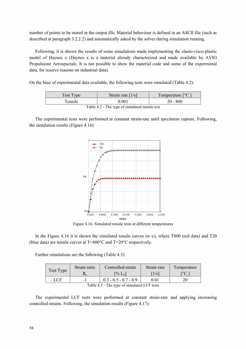
58

number of points to be stored in the output file. Material behaviour is defined in an ASCII file (such as

described at paragraph 3.2.2.2) and automatically asked by the solver during simulation running.

Following, it is shown the results of some simulations made implementing the elasto-visco-plastic

model of Haynes x (Haynes x is a material already characterized and made available by AVIO

Propulsione Aerospaziale. It is not possible to show the material code and some of the expermintal

data, for reserve reasons on industrial data).

On the base of experimental data available, the following tests were simulated (Table 4.2):

Test Type Strain rate [1/s] Temperature [°C ]

Tensile 0.001 20 - 800Table 4.2 - The type of simulated tensile test

The experimental tests were performed at constant strain-rate until specimens rupture. Following,

the simulation results (Figure 4.16):

Figure 4.16- Simulated tensile tests at different temperatures

In the Figure 4.16 it is shown the simulated tensile curves (), where T800 (red data) and T20

(blue data) are tensile curves at T=800°C and T=20°C respectively.

Further simulations are the following (Table 4.3):

Test TypeStrain ratio

R

Controlled-strain

[% L0]

Strain rate

[1/s]

Temperature

[°C ]

LCF -1 0.3 - 0.5 - 0.7 - 0.9 0.01 20Table 4.3 - The type of simulated LCF tests

The experimental LCF tests were performed at constant strain-rate and applying increasing

controlled-strains. Following, the simulation results (Figure 4.17):

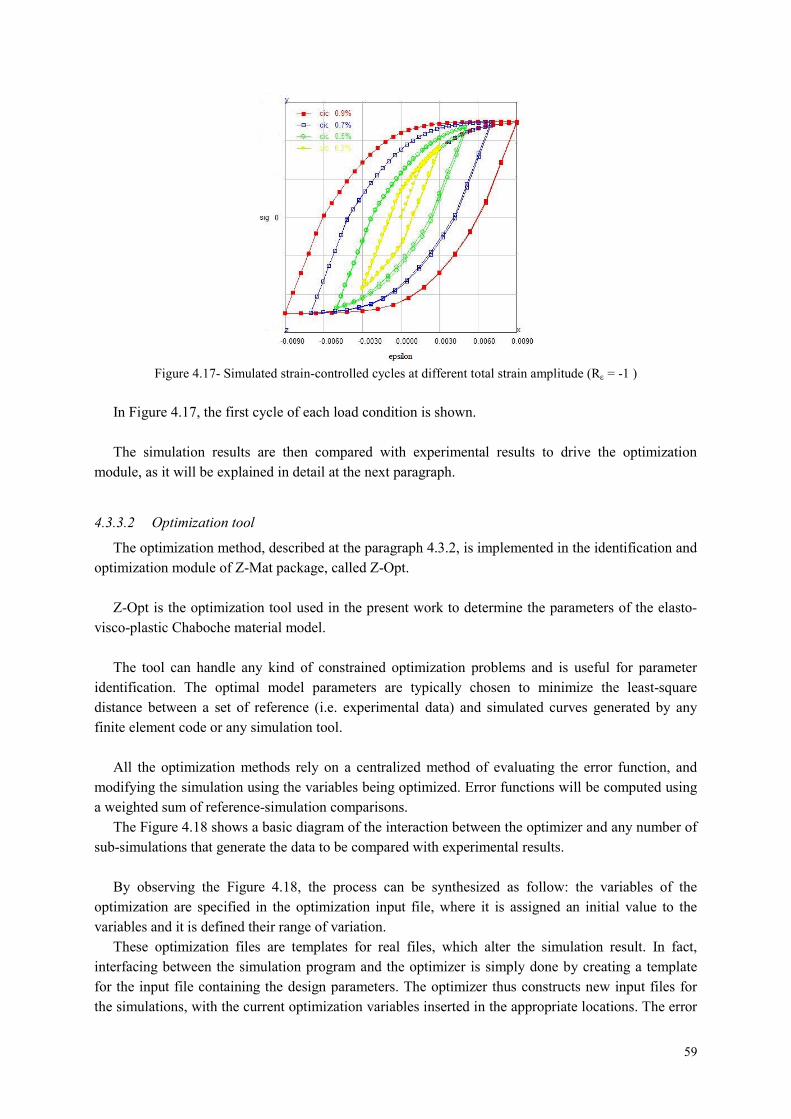
59

Figure 4.17- Simulated strain-controlled cycles at different total strain amplitude (R = -1 )

In Figure 4.17, the first cycle of each load condition is shown.

The simulation results are then compared with experimental results to drive the optimization

module, as it will be explained in detail at the next paragraph.

4.3.3.2 Optimization tool

The optimization method, described at the paragraph 4.3.2, is implemented in the identification and

optimization module of Z-Mat package, called Z-Opt.

Z-Opt is the optimization tool used in the present work to determine the parameters of the elasto-

visco-plastic Chaboche material model.

The tool can handle any kind of constrained optimization problems and is useful for parameter

identification. The optimal model parameters are typically chosen to minimize the least-square

distance between a set of reference (i.e. experimental data) and simulated curves generated by any

finite element code or any simulation tool.

All the optimization methods rely on a centralized method of evaluating the error function, and

modifying the simulation using the variables being optimized. Error functions will be computed using

a weighted sum of reference-simulation comparisons.

The Figure 4.18 shows a basic diagram of the interaction between the optimizer and any number of

sub-simulations that generate the data to be compared with experimental results.

By observing the Figure 4.18, the process can be synthesized as follow: the variables of the

optimization are specified in the optimization input file, where it is assigned an initial value to the

variables and it is defined their range of variation.

These optimization files are templates for real files, which alter the simulation result. In fact,

interfacing between the simulation program and the optimizer is simply done by creating a template

for the input file containing the design parameters. The optimizer thus constructs new input files for

the simulations, with the current optimization variables inserted in the appropriate locations. The error

60

functions are computed by the comparison between simulated curves and experimental ones. New

variables values are available for the next loop until to achieve the best ‘fit’ between the curves and

obtaining in output a set of optimized coefficient.

Figure 4.18- Optimization process

In general, the number of simulation-experiment comparisons will lead the problem to be over-

constrained. It is the optimizer’s job then to find the best fit. If certain experiments are “important”, it

is possible to employ weights on the comparisons functions to make them more dominant in the

function evaluation. Besides, it is important to point out that robust results will be found with many

diverse experiment conditions. Repeated experiments that merely provide a slight variation in

response should be avoided, while complex experiments with many interacting effects should be

emphasized.

The step-by-step procedure just described, foresees adding tests and the corresponding sensitive

parameters progressively into the optimization loop. The previously calibrated coefficients provide

good starting points for the next step, thus allowing the algorithm to escape local minima. At the end,

all tests are added and all coefficients identified at the same time, thus yielding a good quality optimal

set of coefficients.

Following, the results of some simulations and optimizations are shown.

Test Type Strain rate [1/s] Temperature [°C ]

Tensile 0.001 20Table 4.4 - Tensile test

The results of the tensile test (Table 4.4) are shown in the Figure 4.19, where in the graph on the

left it observes the result obtained by the initial simulation (assigning initial coefficients by tentative).

(the blue curve is the experimental data – the red curve is the simulation)

As described at the paragraph 4.3.1, tensile tests allow optimizing the parameters: R0, n, k.

(unknown coefficients involved in this step).

The simulated curve is lower than the experimental one, so other computing loops are necessary to

obtain the best result.

At the end of the optimization iterative process, the coefficients values have been optimized (by

fitting the reference and the simulation) and in the graph on right, it observes the final result. The

experimental curve and the simulation obtained by the optimized model are overlapped.

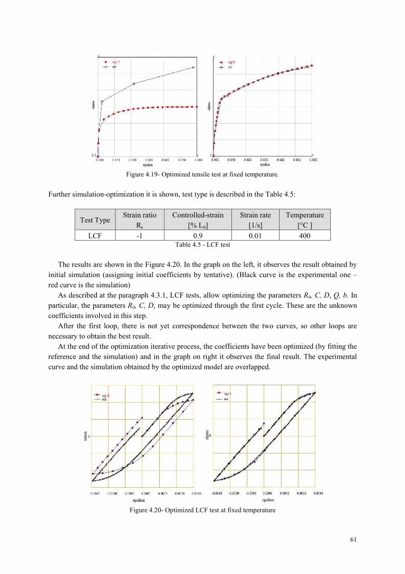
61

Figure 4.19- Optimized tensile test at fixed temperature.

Further simulation-optimization it is shown, test type is described in the Table 4.5:

Test TypeStrain ratio

R

Controlled-strain

[% L0]

Strain rate

[1/s]

Temperature

[°C ]

LCF -1 0.9 0.01 400Table 4.5 - LCF test

The results are shown in the Figure 4.20. In the graph on the left, it observes the result obtained by

initial simulation (assigning initial coefficients by tentative). (Black curve is the experimental one –

red curve is the simulation)

As described at the paragraph 4.3.1, LCF tests, allow optimizing the parameters R0, C, D, Q, b. In

particular, the parameters R0, C, D, may be optimized through the first cycle. These are the unknown

coefficients involved in this step.

After the first loop, there is not yet correspondence between the two curves, so other loops are

necessary to obtain the best result.

At the end of the optimization iterative process, the coefficients have been optimized (by fitting the

reference and the simulation) and in the graph on right it observes the final result. The experimental

curve and the simulation obtained by the optimized model are overlapped.

Figure 4.20- Optimized LCF test at fixed temperature

62

4.3.4 Validation of characterization methodology

The validation of procedure of characterization has been performed through the comparison

between the experimental tests and the tests simulated in ANSYS code, implementing the external

material model.

The first step is to realize FEM models of specimens used for experimental tests.

Subsequently, to apply boundary conditions to the model in way to reproduce the real test

conditions.

To implement the external material model in ANSYS code and to simulate the same tests used for

the material characterization.

By the comparison between the experimental data and material model response, it is possible to

verify the predictive capability of the material model and to validate it.

Following, it is shown how the procedure just described has been applied in order to validate the

coefficients set optimized at the previous paragraph (4.3.3.2).

Referring to the LCF test described in Table 4.5, it has been realized the FEM model of the

specimen used to perform the experimental LCF tests for material characterization. Constraints and

loads have been applied in way to simulate experimental test. The elasto-visco-plastic Chaboche

model with the optimized coefficients has been implemented in ANSYS code and the simulation has

been performed. A detailed description of validation process will be provided to the section 4.4 on the

analysis of experimental data.

The ANSYS simulation of the test described in Table 4.5 and shown in Figure 4.20 has provided

the following result:

-800

-600

-400

-200

0

200

400

600

800

-0,006 -0,004 -0,002 0,000 0,002 0,004 0,006

epsilon [mm/mm]

sig

ma

[MP

a]

Simulated test

Experimental test

Figure 4.21- Comparison between experimental LCF test (1stcycle) and the same test simulated in ANSYS code

The comparison, in Figure 4.21, shows a good agreement between the experimental data and

material model response.

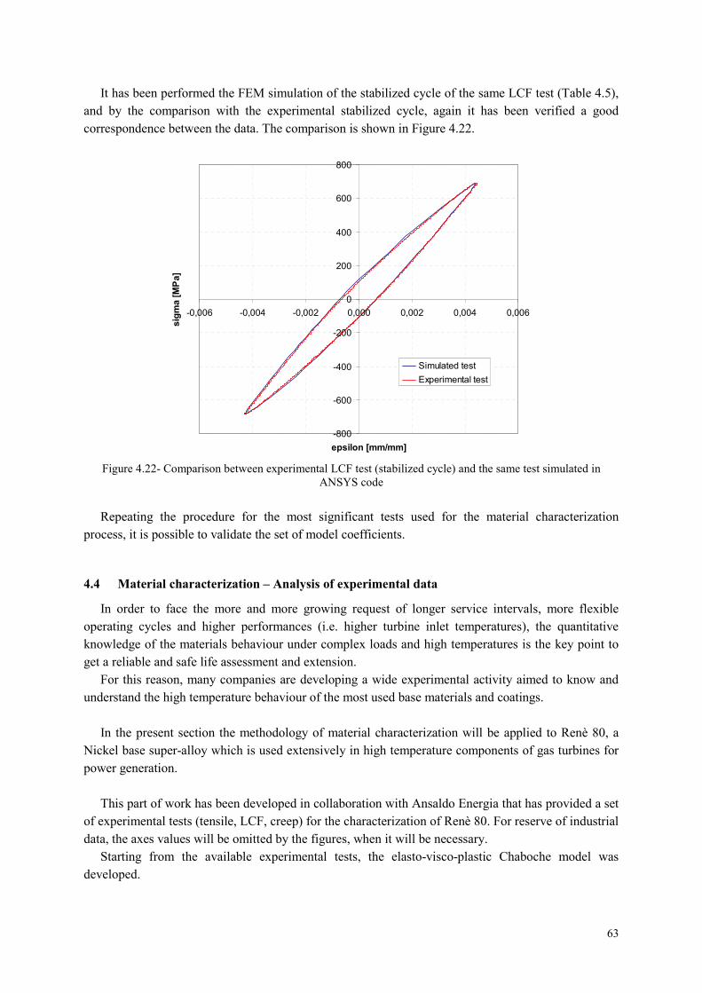
63

It has been performed the FEM simulation of the stabilized cycle of the same LCF test (Table 4.5),

and by the comparison with the experimental stabilized cycle, again it has been verified a good

correspondence between the data. The comparison is shown in Figure 4.22.

-800

-600

-400

-200

0

200

400

600

800

-0,006 -0,004 -0,002 0,000 0,002 0,004 0,006

epsilon [mm/mm]

sig

ma

[MP

a]

Simulated test

Experimental test

Figure 4.22- Comparison between experimental LCF test (stabilized cycle) and the same test simulated inANSYS code

Repeating the procedure for the most significant tests used for the material characterization

process, it is possible to validate the set of model coefficients.

4.4 Material characterization – Analysis of experimental data

In order to face the more and more growing request of longer service intervals, more flexible

operating cycles and higher performances (i.e. higher turbine inlet temperatures), the quantitative

knowledge of the materials behaviour under complex loads and high temperatures is the key point to

get a reliable and safe life assessment and extension.

For this reason, many companies are developing a wide experimental activity aimed to know and

understand the high temperature behaviour of the most used base materials and coatings.

In the present section the methodology of material characterization will be applied to Renè 80, a

Nickel base super-alloy which is used extensively in high temperature components of gas turbines for

power generation.

This part of work has been developed in collaboration with Ansaldo Energia that has provided a set

of experimental tests (tensile, LCF, creep) for the characterization of Renè 80. For reserve of industrial

data, the axes values will be omitted by the figures, when it will be necessary.

Starting from the available experimental tests, the elasto-visco-plastic Chaboche model was

developed.

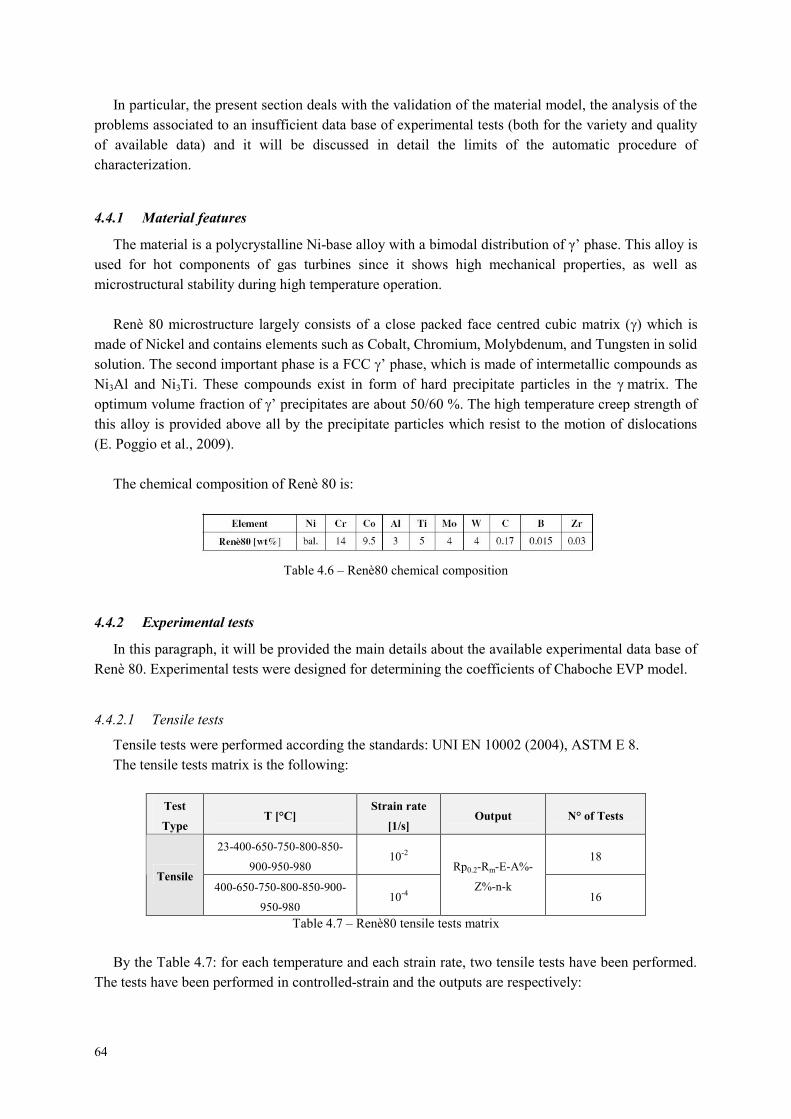
64

In particular, the present section deals with the validation of the material model, the analysis of the

problems associated to an insufficient data base of experimental tests (both for the variety and quality

of available data) and it will be discussed in detail the limits of the automatic procedure of

characterization.

4.4.1 Material features

The material is a polycrystalline Ni-base alloy with a bimodal distribution of γ’ phase. This alloy is

used for hot components of gas turbines since it shows high mechanical properties, as well as

microstructural stability during high temperature operation.

Renè 80 microstructure largely consists of a close packed face centred cubic matrix () which is

made of Nickel and contains elements such as Cobalt, Chromium, Molybdenum, and Tungsten in solid

solution. The second important phase is a FCC ’ phase, which is made of intermetallic compounds as

Ni3Al and Ni3Ti. These compounds exist in form of hard precipitate particles in the matrix. The

optimum volume fraction of ’ precipitates are about 50/60 %. The high temperature creep strength of

this alloy is provided above all by the precipitate particles which resist to the motion of dislocations

(E. Poggio et al., 2009).

The chemical composition of Renè 80 is:

Table 4.6 – Renè80 chemical composition

4.4.2 Experimental tests

In this paragraph, it will be provided the main details about the available experimental data base of

Renè 80. Experimental tests were designed for determining the coefficients of Chaboche EVP model.

4.4.2.1 Tensile tests

Tensile tests were performed according the standards: UNI EN 10002 (2004), ASTM E 8.

The tensile tests matrix is the following:

Test

TypeT [°C]

Strain rate

[1/s]Output N° of Tests

23-400-650-750-800-850-

900-950-98010-2 18

Tensile400-650-750-800-850-900-

950-98010-4

Rp0.2-Rm-E-A%-

Z%-n-k16

Table 4.7 – Renè80 tensile tests matrix

By the Table 4.7: for each temperature and each strain rate, two tensile tests have been performed.

The tests have been performed in controlled-strain and the outputs are respectively:

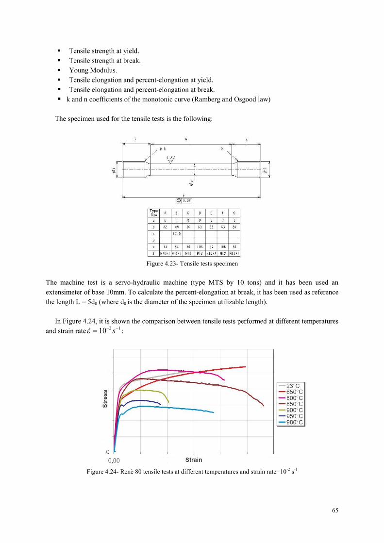
65

Tensile strength at yield.

Tensile strength at break.

Young Modulus.

Tensile elongation and percent-elongation at yield.

Tensile elongation and percent-elongation at break.

k and n coefficients of the monotonic curve (Ramberg and Osgood law)

The specimen used for the tensile tests is the following:

Figure 4.23- Tensile tests specimen

The machine test is a servo-hydraulic machine (type MTS by 10 tons) and it has been used an

extensimeter of base 10mm. To calculate the percent-elongation at break, it has been used as reference

the length L = 5d0 (where d0 is the diameter of the specimen utilizable length).

In Figure 4.24, it is shown the comparison between tensile tests performed at different temperatures

and strain rate 1210 s :

Figure 4.24- Renè 80 tensile tests at different temperatures and strain rate=10-2 s-1

66

By observing the Figure 4.24: the tests have been performed until the specimen break. The yield

stress has higher values between T=650°C and T=900°C, even if the absolute maximum value is

obtained at T=23°C. The maximum tensile strength at break is obtained at T=650°C

Besides, by the Figure 4.24 it is possible to observe an anomalous material behaviour at

temperatures around T=800°C. It shows an increasing of stresses with the increasing of temperature in

the range of temperatures between T=650°C – 800°C.

The anomalous behaviour may be explained by a microstructural point of view, since the material

changes its state around T=800°C.

In Figure 4.25, it is shown the comparison between tensile tests performed at different temperatures

and strain rate 1410 s :

Figure 4.25- Renè80 tensile tests at different temperatures and strain rate=10-4 s-1

By observing the Figure 4.25: the tests have been performed until the specimen break. The yield

stress has higher value at T=400°C. The relative maximum of tensile strength at break is obtained

around T=650°C

4.4.2.2 LCF tests

LCF tests have been performed according the standards ASTM E 606.

The LCF tests matrix is the following:

Test

TypeT [°C]

Strain rate

[1/s]

Strain ratio R

Controlled-strainOutput N° of Tests

400-800-900 10-2 R= -1; 6 levels of 18

LCF900 10-2

R= -1; 2 levels of

’ hold time

Hysteresis cycle;

max and min =f(N);

cyclic curve;

stabilized curve;

% = f(N)

2

Table 4.8 – Renè80 LCF tests matrix

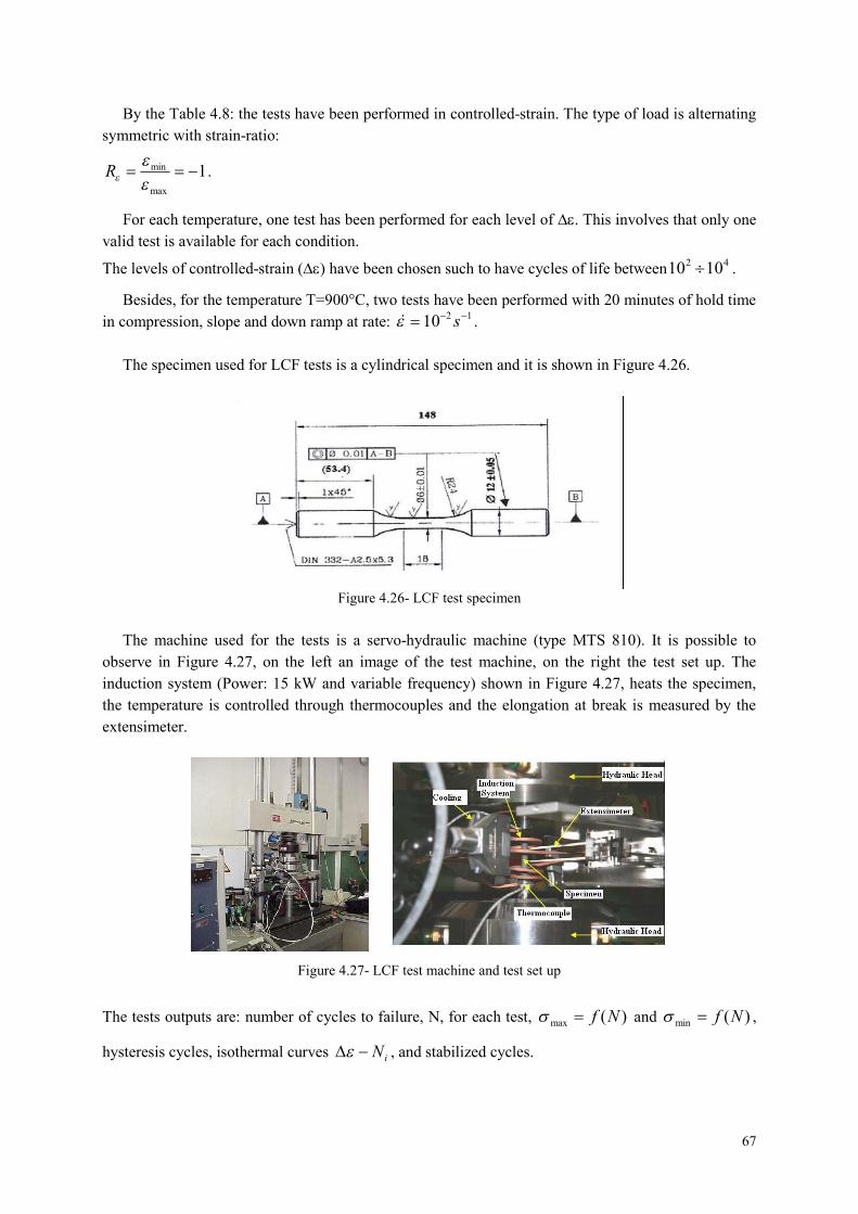
67

By the Table 4.8: the tests have been performed in controlled-strain. The type of load is alternating

symmetric with strain-ratio:

1max

min

R .

For each temperature, one test has been performed for each level of . This involves that only one

valid test is available for each condition.

The levels of controlled-strain ( have been chosen such to have cycles of life between 42 1010 .

Besides, for the temperature T=900°C, two tests have been performed with 20 minutes of hold time

in compression, slope and down ramp at rate: 1210 s .

The specimen used for LCF tests is a cylindrical specimen and it is shown in Figure 4.26.

Figure 4.26- LCF test specimen

The machine used for the tests is a servo-hydraulic machine (type MTS 810). It is possible to

observe in Figure 4.27, on the left an image of the test machine, on the right the test set up. The

induction system (Power: 15 kW and variable frequency) shown in Figure 4.27, heats the specimen,

the temperature is controlled through thermocouples and the elongation at break is measured by the

extensimeter.

Figure 4.27- LCF test machine and test set up

The tests outputs are: number of cycles to failure, N, for each test, )(max Nf and )(min Nf ,

hysteresis cycles, isothermal curves iN , and stabilized cycles.

68

In Figure 4.28 it is shown the fatigue curve at T = 800°C: total controlled-strain versus number of

cycles to failure, in logarithmic scale. In the same figure, it is shown also the equation obtained

through exponential regression.

LCF, Renè 80, 800°C

y = 2,3658x-0,168

R2

= 0,9716

10 100 1000 10000

N, Cycles to Failure

Tot

alS

trai

nR

ange

,%

Figure 4.28- Fatigue curve at T=800°C

In the Figure 4.29, it is shown the hysteresis cycle obtained for the LCF test performed at T=900°C

and % = 0.99. In particular, it is shown the first and the stabilized cycles, used in the material

characterization process for determining kinematic and isotroping hardening coefficients of Chaboche

model.

-0,006 -0,004 -0,002 0 0,002 0,004 0,006

epsilon [mm/mm]

sig

ma

[MP

a]

First cycle

Stabilized cicle

Figure 4.29- Hysteresis cycles - LCF test at T=900°C and % = 0.99

Moreover, in order to know after how many cycles the material behaviour is stabilized, it is

necessary to calculate the curves:

)(max Nf and )(min Nf

In fact, when the values of max and min do not change between the previous cycle and the next

one, the material behaviour is stabilized.

69

In Figure 4.30, it is shown the curve max versus number of cycles obtained by the LCF test at

T=900°C and % = 0.99. The material stabilization is achieved around to the 15th cycle. The

decreasing of the maximum stress observed in the final part of the curve, is due to the fact that the test

is performed until the specimen failure.

0 20 40 60 80 100 120 140 160 180 200

N of cycles

sig

ma

max

[MP

a]

Figure 4.30 – Curve max vs N - LCF test at T=900°C and % = 0.99 -

Finally, by the stabilized cycles, the cyclic curve of material has been determined such as explained

at the paragraph 4.2.3, in order to evaluate the cyclic material response. In fact, by the comparison

between the monotonic curve and cyclic curve (in particular observing the relative position between

them) it is possible to evaluate the hardening (or softening) material behaviour. This is one of the first

information necessary in the material characterization process.

In Figure 4.31, it is shown the material cyclic curve determined for T=800°C:

Total strain

Str

ess

LCF - stabilized cycles

Ramberg and Osgood equation

Figure 4.31- Cyclic curve at T = 800°C

In particular, in Figure 4.31 the stabilized cycles peaks of the tests performed at different levels of

controlled-strain have been interpolating with Ramberg-Osgood equation (4.3). The result is the cyclic

curve.

70

4.4.2.3 LCF - step tests

For determining the Chaboche model of Renè 80, LCF step tests are necessary in addition to the

LCF traditional ones (LCF duration tests). Each specimen is submitted to steps of N cycles performed

at increasing levels of controlled-strain () and two strain rates. At the end of steps

the specimen have not to be failure since the material have to be submitted to a relaxation.

In the Table 4.9 the matrix of LCF step tests:

T [°C]Test Type

Controlled

strainCycles

Strain rate

[1/s] 400 800 900

20 10-2

20 10-4

20 10-2

20 10-4

20 10-2

20 10-4

20 10-2

LC

F-

Ste

p

20 10-4

2tests 2tests 2tests

Table 4.9 - Renè80 - LCF step tests matrix

The outputs of LCF step tests are the same of LCF duration tests. In addition, the stress relaxation

curve is provided for each test condition.

In Figure 4.32 it is shown the result of LCF step test at T=900°C. In particular, it is shown the max

and min curves versus the number of cycles.

0 50 100 150 200

N of cycles

Str

ess

[MP

a]

Stress max

Stress min

Figure 4.32- LCF step test at T=900°C

In Figure 4.33, it is shown the stress relaxation curve obtained from the same LCF step test

performed at T=900°C. The last level of controlled-strain was held constant for one hour, to obtain a

stress relaxation.

71

0 500 1000 1500 2000 2500 3000 3500 4000

Time [s]

Str

ess

[Mp

a]

Figure 4.33- Stress relaxation at T=900°C

4.4.2.4 Creep tests

Creep tests were performed according the standards ASTM E 139, EN10291.

The creep tests matrix is the following:

Test

TypeT [°C] Controlled stress Output N° of Tests

Creep 800-850-900-950 5 levels of

tu ; f(t) ; R ; AR ;

creep strain rate ;

minimum strain rate

20

Table 4.10 - Renè80 – Creep tests matrix

The specimen is subjected to a constant state of stress and the resulting variation in strain, as a

function of time, is determined.

Four temperatures and five levels of load were examined (Table 4.10). In particular, the range of

temperatures has been chosen in way to be the most representative of the real conditions of the

components during service. The levels of load have been chosen to have failure times well distributed

in the range of interest (300-10000 hours).

The test outputs are (Table 4.10):

Time to failure

Creep curve: strain versus time

Strain and elongation at break (R ; AR)

Creep strain rate and minimum creep strain rate.

Creep tests specimen is shown in Figure 4.34.

72

Figure 4.34- Creep tests specimen

Two extensometers have been used for monitoring the strain in the specimen utilizable length

during the test. Three thermocouples have been applied along the axis of the specimen utilizable

length to control the temperature.

The strain has been calculated by:

0l

l (4.17)

Where: l0 and l are respectively the specimen utilizable length and its elongation during creep test.

The accumulated plastic strain has been calculated as follows:

Etotp

(4.18)

Where tot is the total strain cumulated during the loading phase.

Following, some results of creep tests.

In Figure 4.35, it is shown the time to failure measured for each test (for each level of load). The

graph time to failure versus stress is in logarithmic scale and at different temperatures.

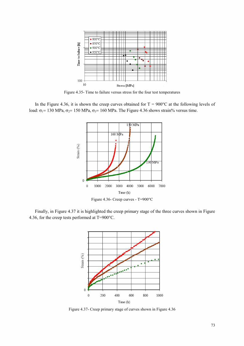
73

Figure 4.35- Time to failure versus stress for the four test temperatures

In the Figure 4.36, it is shown the creep curves obtained for T = 900°C at the following levels of

load: 130 MPa, 150 MPa, 160 MPa. The Figure 4.36 shows strain% versus time.

Figure 4.36- Creep curves - T=900°C

Finally, in Figure 4.37 it is highlighted the creep primary stage of the three curves shown in Figure

4.36, for the creep tests performed at T=900°C.

Figure 4.37- Creep primary stage of curves shown in Figure 4.36

74

4.4.3 Elasto-visco-plastic behaviour model of Renè 80

Chaboche model described at paragraphs 2.9.1 and 4.2.5 was chosen for modelling the elasto-

visco-plastic behaviour of Renè 80.

The viscoplasticity with isotropic and kinematic hardening combines plasticity and creep and

allows taking into account of the rate dependence. Besides, it let stresses outside of yield relax if there

is not further straining.

A multi-kinematic hardening mechanism was chosen (Lemaitre and Chaboche, 1990):

RXJf i (4.19)

In which the kinematic variables Xi are independent and obey to an evolution rule such that:

dpXDdCdX iip

ii 3

2(4.20)

Where: p is the present plastic strain and p is the accumulated plastic strain.

The necessity to introduce a multi-kinematic hardening mechanism was due to the wide range of

changes in strain shown by LCF tests. In this case, one kinematic hardening mechanism was not

sufficient to describe the transition from linear to nonlinear material behaviour. In fact, for very low

strains, one recovered the linear case with a poor representation of the elasto-plastic transition and for

high strains, the limiting value was reached very rapidly. For remedying to such deficiency, two

kinematic hardening mechanisms were superimposed.

An example of the results obtained by the implementation of multiple kinematic hardening

mechanisms is shown in the following figure:

Figure 4.38- Multi-kinematic hardening mechanism

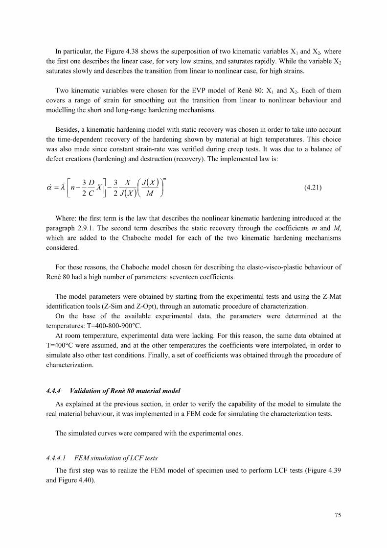
75

In particular, the Figure 4.38 shows the superposition of two kinematic variables X1 and X2, where

the first one describes the linear case, for very low strains, and saturates rapidly. While the variable X2

saturates slowly and describes the transition from linear to nonlinear case, for high strains.

Two kinematic variables were chosen for the EVP model of Renè 80: X1 and X2. Each of them

covers a range of strain for smoothing out the transition from linear to nonlinear behaviour and

modelling the short and long-range hardening mechanisms.

Besides, a kinematic hardening model with static recovery was chosen in order to take into account

the time-dependent recovery of the hardening shown by material at high temperatures. This choice

was also made since constant strain-rate was verified during creep tests. It was due to a balance of

defect creations (hardening) and destruction (recovery). The implemented law is:

m

M

XJ

XJ

XX

C

Dn

2

3

2

3 (4.21)

Where: the first term is the law that describes the nonlinear kinematic hardening introduced at the

paragraph 2.9.1. The second term describes the static recovery through the coefficients m and M,

which are added to the Chaboche model for each of the two kinematic hardening mechanisms

considered.

For these reasons, the Chaboche model chosen for describing the elasto-visco-plastic behaviour of

Renè 80 had a high number of parameters: seventeen coefficients.

The model parameters were obtained by starting from the experimental tests and using the Z-Mat

identification tools (Z-Sim and Z-Opt), through an automatic procedure of characterization.

On the base of the available experimental data, the parameters were determined at the

temperatures: T=400-800-900°C.

At room temperature, experimental data were lacking. For this reason, the same data obtained at

T=400°C were assumed, and at the other temperatures the coefficients were interpolated, in order to

simulate also other test conditions. Finally, a set of coefficients was obtained through the procedure of

characterization.

4.4.4 Validation of Renè 80 material model

As explained at the previous section, in order to verify the capability of the model to simulate the

real material behaviour, it was implemented in a FEM code for simulating the characterization tests.

The simulated curves were compared with the experimental ones.

4.4.4.1 FEM simulation of LCF tests

The first step was to realize the FEM model of specimen used to perform LCF tests (Figure 4.39

and Figure 4.40).

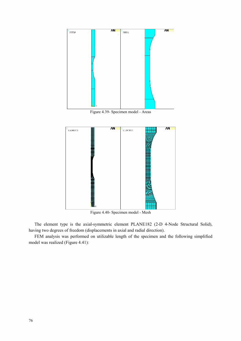
76

Figure 4.39- Specimen model - Areas

Figure 4.40- Specimen model - Mesh

The element type is the axial-symmetric element PLANE182 (2-D 4-Node Structural Solid),

having two degrees of freedom (displacements in axial and radial direction).

FEM analysis was performed on utilizable length of the specimen and the following simplified

model was realized (Figure 4.41):

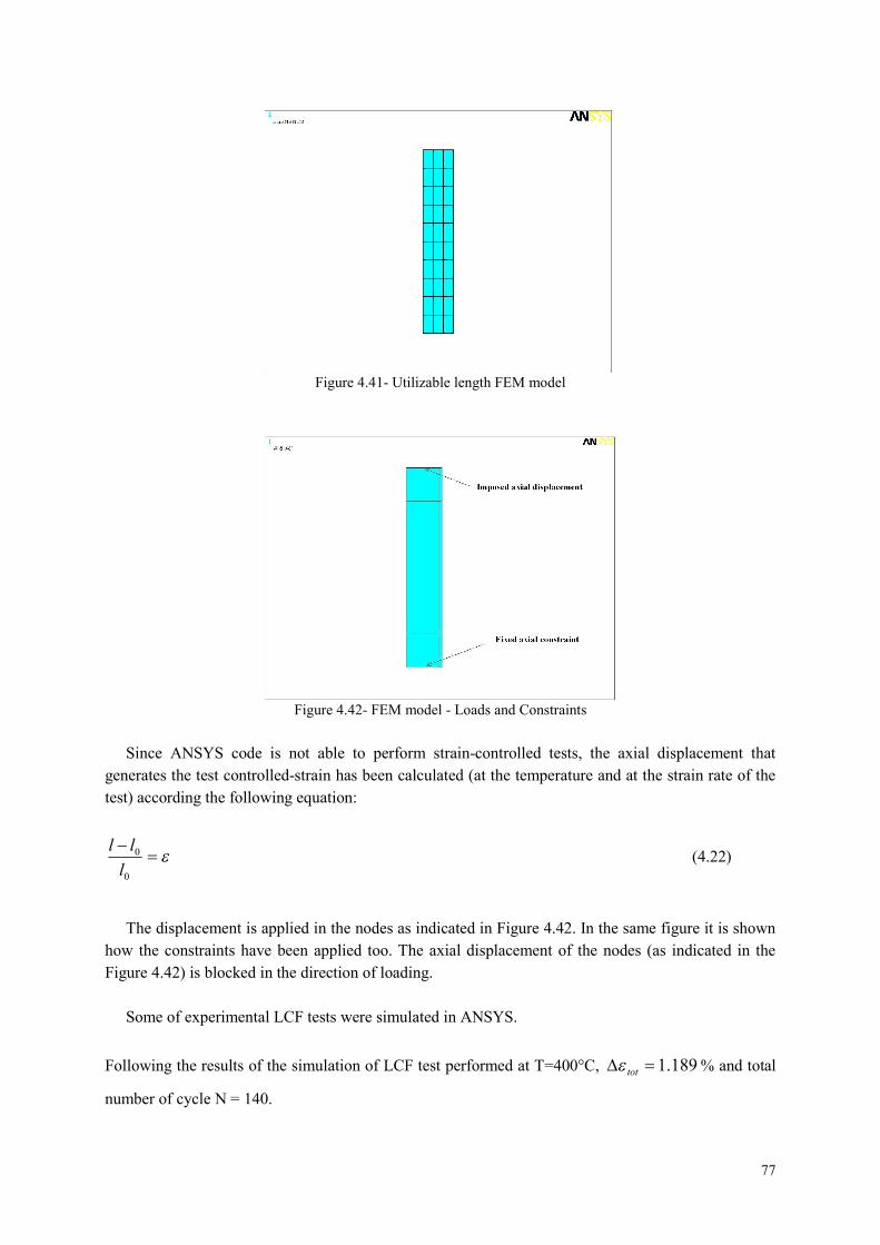
77

Figure 4.41- Utilizable length FEM model

Figure 4.42- FEM model - Loads and Constraints

Since ANSYS code is not able to perform strain-controlled tests, the axial displacement that

generates the test controlled-strain has been calculated (at the temperature and at the strain rate of the

test) according the following equation:

0

0

l

ll(4.22)

The displacement is applied in the nodes as indicated in Figure 4.42. In the same figure it is shown

how the constraints have been applied too. The axial displacement of the nodes (as indicated in the

Figure 4.42) is blocked in the direction of loading.

Some of experimental LCF tests were simulated in ANSYS.

Following the results of the simulation of LCF test performed at T=400°C, 189.1 tot % and total

number of cycle N = 140.

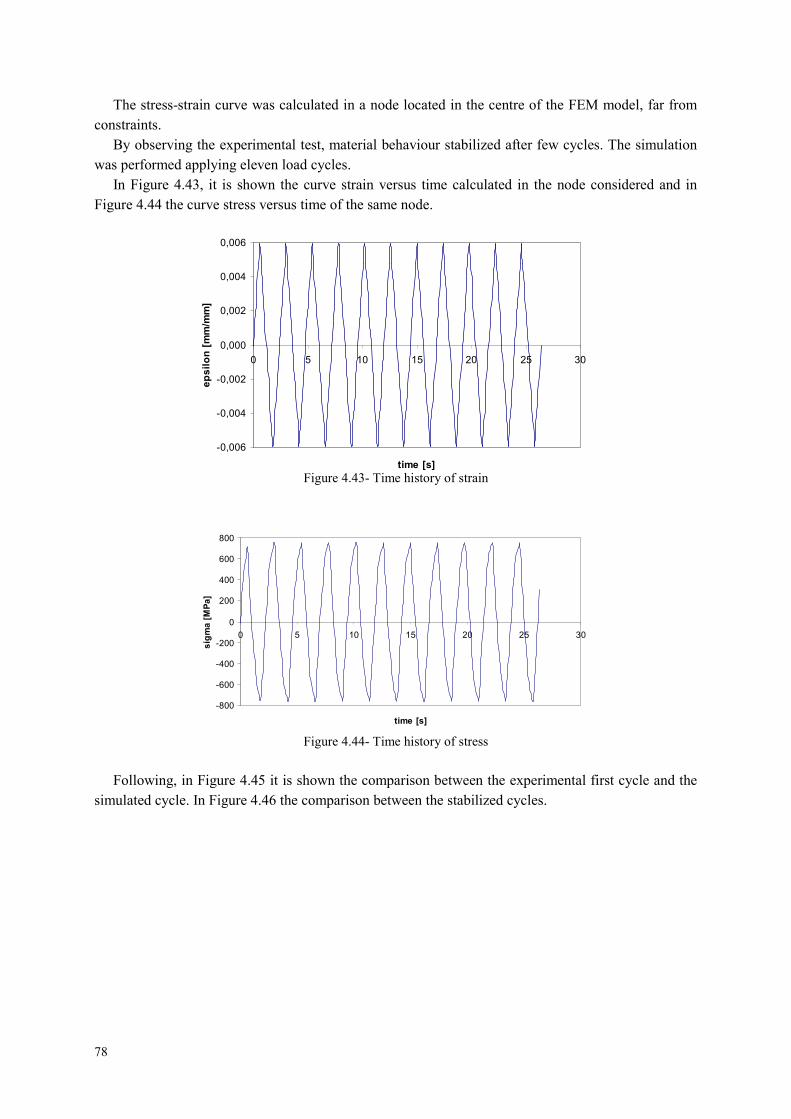
78

The stress-strain curve was calculated in a node located in the centre of the FEM model, far from

constraints.

By observing the experimental test, material behaviour stabilized after few cycles. The simulation

was performed applying eleven load cycles.

In Figure 4.43, it is shown the curve strain versus time calculated in the node considered and in

Figure 4.44 the curve stress versus time of the same node.

-0,006

-0,004

-0,002

0,000

0,002

0,004

0,006

0 5 10 15 20 25 30

time [s]

ep

sil

on

[mm

/mm

]

Figure 4.43- Time history of strain

-800

-600

-400

-200

0

200

400

600

800

0 5 10 15 20 25 30

time [s]

sig

ma

[MP

a]

Figure 4.44- Time history of stress

Following, in Figure 4.45 it is shown the comparison between the experimental first cycle and the

simulated cycle. In Figure 4.46 the comparison between the stabilized cycles.

79

-800

-600

-400

-200

0

200

400

600

800

-0,008 -0,006 -0,004 -0,002 0 0,002 0,004 0,006 0,008

epsilon [mm/mm]

sig

ma

[MP

a]

Simulation_cycle n° 1

Experimental_cycle n° 1

Figure 4.45- Comparison between the first cycle of LCF experimental test and the simulated one

-800

-600

-400

-200

0

200

400

600

800

-0,008 -0,006 -0,004 -0,002 0,000 0,002 0,004 0,006 0,008

epsilon [mm/mm]

sig

ma

[MP

a]

Simulated cycle

Experimental cycle

Figure 4.46- Comparison between the stabilized cycle of LCF experimental test and the simulated one

The comparisons shown in Figure 4.45 and Figure 4.46 illustrate a good predictive capability of the

model for the stabilized material behaviour, differently for the first cycle.

All the comparisons performed between LCF experimental tests and simulated ones have shown a

good correspondence on the stabilized cycle, while differences have been highlighted on first cycle. In

particular, the model response is not sufficient to describe correctly the transition from linear to non-

linear material behaviour.

4.4.4.2 FEM simulation of creep tests

The first step was to realize the FEM model of specimen used to perform creep tests (Figure 4.47

and Figure 4.48).

80

Figure 4.47- Specimen model - Areas

Figure 4.48- Specimen model - Mesh

The element type is the axial symmetric element PLANE182 (2-D 4-Node Structural Solid), having

two degrees of freedom (displacements in axial and radial direction).

FEM analysis was performed on utilizable length of the specimen and the following simplified

model was realized:

Figure 4.49- Utilizable length FEM model

Loads and constraints were applied as shown in Figure 4.50:

81

Figure 4.50- FEM model - Loads and Constraints

Some of experimental creep tests were simulated in ANSYS.

Following, in Figure 4.51, the results of the analysis that simulates the creep test performed at

T=800°C and = 290 MPa.

0

0,05

0,1

0,15

0,2

0,25

0,3

0,35

0,4

0 100 200 300 400 500 600

time [hour]

str

ain

%

Experimental

Simulation

Figure 4.51- Comparison between experimental creep test and simulated one

The creep curve (Figure 4.51), time expressed in hours versus strain%, was calculated in a node

located in the centre of the FEM model, far from constraint.

The comparison, shown in Figure 4.51, illustrates a not sufficient predictive capability of the model

for the creep material behaviour.

4.5 Limits of the automatic procedure of characterization

The most important and difficult aspect of modeling material behaviour at elevated temperature is

to obtain the required material functions for viscoplaticity and associated material parameters.

The complexity of this process typically stems from not only the variety in mathematical forms for

the material functions, but also from the fact that given the material functions there is no unique set of

material parameters for any given load path. Therefore, numerous iterations and difficult compromises

82

are required before a final set of material parameters (for the assumed material functions) can be

obtained.

Traditionally, characterization has been accomplished through basic trial and error procedures (i.e.,

graphical and/or mechanistic) which attempt to fit the predicted response from the constitutive model

to that response exhibited by the experimental test data. These approaches, however, are rather limited,

difficult, and many times less than fruitful for more general and sophisticated constitutive models.

This is particularly true when dealing whit models that possesses a very large number of material

constants that:

are often lacking in their direct physical interpretation

may have vastly different magnitudes

are highly interactive with each other.

Further complications also arise when a large number of experimental tests of various types under

transient and/or steady-state conditions, are expected to be simulated.

Besides, a model must have a general character, so that while identified only by a restricted number

of experiments, it is representative of other types of experiments with a predictive capability.

The totality of the situations verified by a model is its field of validity. The goodness of the model

is expressed qualitatively by the set of all possible variation histories of the variables and

quantitatively by the range of the variations within which the model agrees with the physics.

A given model cannot be identified correctly unless a sufficient number of test results are available,

which embrace a significant range of variation of each parameter. Otherwise, one runs the risk of not

determining one or more coefficients well enough.

The number of coefficients represents the price to pay, since the difficulties of identification

essentially lie in this number and for this reason it is necessary to turn to the computer aided

identification.

As shown previously, software tools as Z-Sim and Z-Opt have been developed to enable a design

engineer to bridge this gap between constitutive theory and experimental test data, in which optimum

material parameters have to be determined by minimizing the errors between experimental data and

the correlated responses.

The main difficulties associated with the use of complex constitutive equations to predict the

behaviour of high temperature components are:

Number of parameters

Quality of performed experiments

The aim of this part of work is to show the limits of an automatic procedure of material

characterization and how the process is affected by the available experimental data.

4.5.1 High number of coefficients and problems of solution convergence

One of the main difficulties found in the process of Renè 80 characterization was in the

identification of the high number of model coefficients.

83

In this model, two potentials have been defined in order to take into account the different

mechanisms of material deformation associated with a wide range of strain rates.

For the first potential:

two coefficients for Norton law which describe the viscous behavior (K, n)

three coefficients for modeling the non linear isotropic hardening mechanism (R0, Q, b)

four coefficients for modeling the two nonlinear hardening kinematic mechanisms (C1,D1 and

C2,D2)

four coefficients for describing the recovery of the hardening at high temperatures (m1, M1

and m2, M2)

For the second potential:

two coefficients for Norton law (K, n)

one coefficient for isotropic constant hardening (R0)

Other two model coefficients are Young and Poisson Modulus for describing the linear elastic

behaviour.

In these cases, it is strongly advised to use a step-by-step procedure of characterization, adding

tests and the corresponding sensitive parameters progressively into the optimization loop. In such

procedure, the previously calibrated coefficients provide good starting points for the next step, thus

allowing the algorithm to escape from local minima. Finally, all tests have to be added and all

coefficients identified at the same time, for obtaining a good set of coefficients.

In spite of a step by step procedure was applied, many problems of convergence of the optimization

tool were verified.

Many coefficients in fact are strongly depending each other and, in absence of a good experimental

data base, a non correct identification of one of them, implies the not convergence of the solution

during the optimization process.

This has been verified during the identification of the parameters R0 and k. They represent

respectively initial yield stress and viscous stress. For determining them, it is necessary an

experimental data base which includes many tensile tests at different temperatures and strain rates.

Later, it will be shown the available data were not sufficient. For this reason, it was not possible to

optimize those parameters. Even forcing the tool and inserting "by hand" the real value of R0 (the

initial yield stress read by the first cycle of the LCF test), it wasn't possible to obtain the optimized

value of k, since the solution didn't converge.

4.5.2 Quality and variety of experimental tests

Further critical aspect on which to focus on the attention is to have at disposal a “correct”

experimental data base.

A correct data base implies variety of experimental data not just quantity. In other words, if one

only provides tensile data to the optimization tool for determining the coefficients of the model, one

should not expect the model to be able to accurately predict both creep and relaxation response (since

the time duration of these types of tests far exceeds that of a tensile test). Similarly, if one provides

84

only creep or relaxation data to the tool, one should not expect the model to accurately represent the

typically shorter time domain tensile behavior of the material.

Besides a correct data base means also dependable experimental data, proved by a sufficient

number of repetitions for each test.

A detailed analysis of the available experimental data base was performed. It led to conclude that

the data were not sufficient for obtaining an optimized set of parameters and modeling Renè 80

behaviour.

Following, an analysis of the experimental tensile data base.

As seen, at the same temperature two tests are available for each strain-rate. It was verified that

some tests performed at the same conditions (temperature and strain-rate), show a different behavior

and in particular Young modulus is different (Figure 4.52).

0,000 0,005 0,010 0,015 0,020 0,025 0,030 0,035 0,040 0,045

epsilon [mm/mm]

sig

ma

[MP

a]

Figure 4.52- Comparison between two tensile tests at the same temperature and strain rate

As well as, some tests performed at the same temperature and at different strain rate (v = 10-2 s-1

and v= 10-4 s-1) show different Young modulus (Figure 4.53):

85

0,000 0,005 0,010 0,015 0,020 0,025 0,030 0,035 0,040 0,045

epsilon [mm/mm]

sig

ma

[MP

a]

test at v = 10-4 [s-1]

test at v = 10-2 [s-1]

Figure 4.53- Comparison between two tensile tests at the same temperature and different strain rate

In these cases, a further test for each condition (to have a statistically sufficient data base) would

allow validating each test.

Besides, a further anomaly has been verified in tensile data base at T=900°C: the two tests

performed respectively at strain rates: v = 10-2 s-1 and v= 10-4 s-1 show a yield stress of different order

of magnitude. In particular, the test at v = 10-2 s-1 shows a yield stress twice higher of the one at v= 10-

4 s-1 (Figure 4.54).

It is important to highlight that the sensitivity to strain-rate is correct, but the difference have to be of

the order of magnitude 2010 MPa.

0,000 0,005 0,010 0,015 0,020 0,025 0,030 0,035 0,040 0,045 0,050

epsilon [mm/mm]

sig

ma

[MP

a]

Test at v = 10-2 [s-1]

Test at v = 10-4 [s-1]

Figure 4.54- Comparison between tensile tests at T=900°C and different strain rates

Moreover, tensile tests are not according with other experimental data. The comparison between

the tensile tests and the first cycle of LCF tests performed in the same condition shows a different

behaviour.

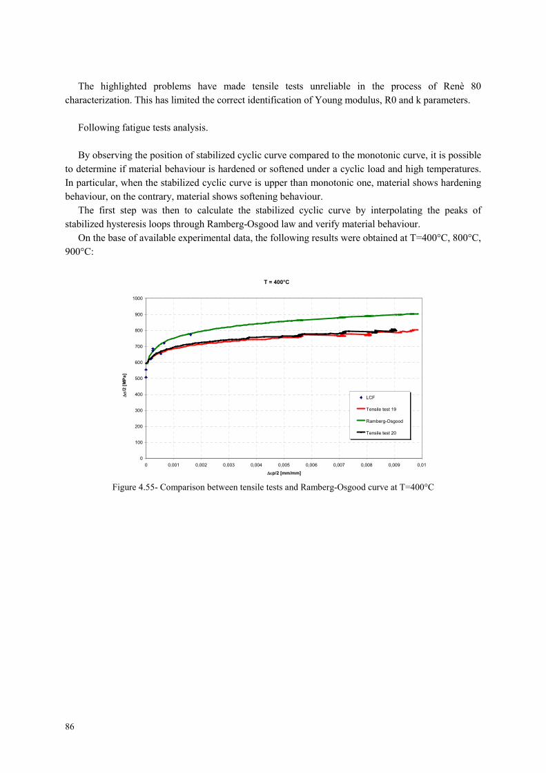
86

The highlighted problems have made tensile tests unreliable in the process of Renè 80

characterization. This has limited the correct identification of Young modulus, R0 and k parameters.

Following fatigue tests analysis.

By observing the position of stabilized cyclic curve compared to the monotonic curve, it is possible

to determine if material behaviour is hardened or softened under a cyclic load and high temperatures.

In particular, when the stabilized cyclic curve is upper than monotonic one, material shows hardening

behaviour, on the contrary, material shows softening behaviour.

The first step was then to calculate the stabilized cyclic curve by interpolating the peaks of

stabilized hysteresis loops through Ramberg-Osgood law and verify material behaviour.

On the base of available experimental data, the following results were obtained at T=400°C, 800°C,

900°C:

T = 400°C

0

100

200

300

400

500

600

700

800

900

1000

0 0,001 0,002 0,003 0,004 0,005 0,006 0,007 0,008 0,009 0,01

p/2 [mm/mm]

/2[M

Pa

]

LCF

Tensile test 19

Ramberg-Osgood

Tensile test 20

Figure 4.55- Comparison between tensile tests and Ramberg-Osgood curve at T=400°C

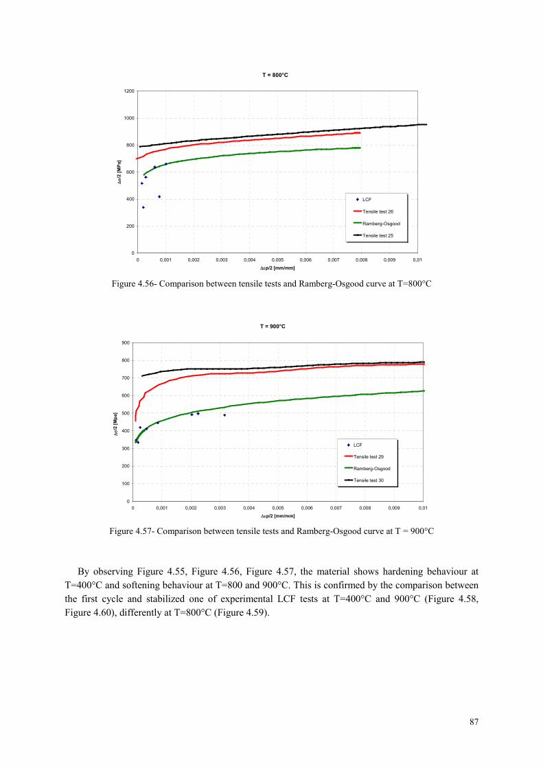
87

T = 800°C

0

200

400

600

800

1000

1200

0 0,001 0,002 0,003 0,004 0,005 0,006 0,007 0,008 0,009 0,01

p/2 [mm/mm]

/2[M

Pa]

LCF

Tensile test 26

Ramberg-Osgood

Tensile test 25

Figure 4.56- Comparison between tensile tests and Ramberg-Osgood curve at T=800°C

T = 900°C

0

100

200

300

400

500

600

700

800

900

0 0,001 0,002 0,003 0,004 0,005 0,006 0,007 0,008 0,009 0,01

p/2 [mm/mm]

/2[M

pa]

LCF

Tensile test 29

Ramberg-Osgood

Tensile test 30

Figure 4.57- Comparison between tensile tests and Ramberg-Osgood curve at T = 900°C

By observing Figure 4.55, Figure 4.56, Figure 4.57, the material shows hardening behaviour at

T=400°C and softening behaviour at T=800 and 900°C. This is confirmed by the comparison between

the first cycle and stabilized one of experimental LCF tests at T=400°C and 900°C (Figure 4.58,

Figure 4.60), differently at T=800°C (Figure 4.59).

88

T = 400°C

-0,006 -0,004 -0,002 0 0,002 0,004 0,006

epsilon [mm/mm]

sig

ma

[Mp

a]

LCF test_cycle 1

LCF test_stabilizedcycle

Figure 4.58- LCF test at T=400°C - First cyclic and stabilized cycle

T = 800°C

-0,006 -0,004 -0,002 0 0,002 0,004 0,006

epsilon [mm/mm]

sigm

a[M

pa

]

LCF test _cycle 1

LCF test_ stabilized cycle

Figure 4.59- LCF test at T=800°C - First cyclic and stabilized cycle

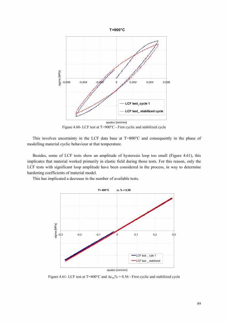
89

T=900°C

-0,006 -0,004 -0,002 0 0,002 0,004 0,006

epsilon [mm/mm]

sig

ma

[MP

a]

LCF test_cycle 1

LCF test_ stabilized cycle

Figure 4.60- LCF test at T=900°C - First cyclic and stabilized cycle

This involves uncertainty in the LCF data base at T=800°C and consequently in the phase of

modelling material cyclic behaviour at that temperature.

Besides, some of LCF tests show an amplitude of hysteresis loop too small (Figure 4.61), this

implicates that material worked primarily in elastic field during those tests. For this reason, only the

LCF tests with significant loop amplitude have been considered in the process, in way to determine

hardening coefficients of material model.

This has implicated a decrease in the number of available tests.

T= 400°C % = 0,56

-0,3 -0,2 -0,1 0 0,1 0,2 0,3

epsilon [mm/mm]

sig

ma

[MP

a]

LCF test _ cyle 1

LCF test _ stabilizedcycle

Figure 4.61- LCF test at T=400°C and tot% = 0.56 - First cyclic and stabilized cycle

90

T=800°C - % = 0.57

-0,003 -0,002 -0,001 0 0,001 0,002 0,003

Epsilon [mm/mm]

Sig

ma

[MP

a]

LCF Test_Cycle1

LCF Test_Stabilized Cycle

Figure 4.62- LCF test at T=800°C and tot% = 0.57 - First cyclic and stabilized cycle

Moreover, further anomaly was found in LCF data base: some tests show values of Young modulus

too scattered at the same temperature.

LCF Tests - Young Modulus

R2

= 0,5853

0 100 200 300 400 500 600 700 800 900 1000

T [°C]

Youn

gM

odu

lus

[GP

a]

Figure 4.63- LCF tests – Young modulus versus Temperature

This, probably, is due to a non-homogeneous structure of material with the presence of grains of

big size and macroscopic area of dendritic solidification. This has affected the process of material

characterization, since the model is very sensitive to the Young modulus variations, as described

following.

The comparison between the first cycle of the experimental LCF test at T=400°C and 0.75

and the simulation of the same cycle in Z-Sim is shown:

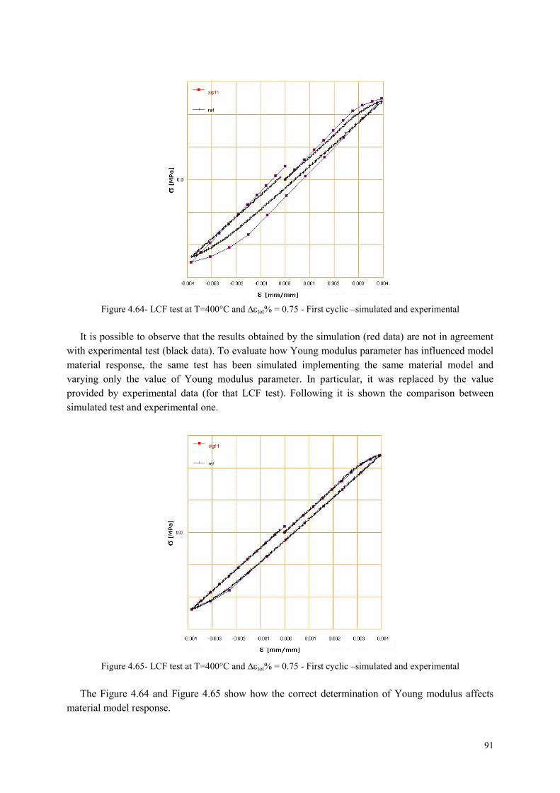
91

Figure 4.64- LCF test at T=400°C and tot% = 0.75 - First cyclic –simulated and experimental

It is possible to observe that the results obtained by the simulation (red data) are not in agreement

with experimental test (black data). To evaluate how Young modulus parameter has influenced model

material response, the same test has been simulated implementing the same material model and

varying only the value of Young modulus parameter. In particular, it was replaced by the value

provided by experimental data (for that LCF test). Following it is shown the comparison between

simulated test and experimental one.

Figure 4.65- LCF test at T=400°C and tot% = 0.75 - First cyclic –simulated and experimental

The Figure 4.64 and Figure 4.65 show how the correct determination of Young modulus affects

material model response.

92

The scattered values of Young modulus provided by experimental LCF tests and the uncertainties

previously highlighted in experimental tensile tests represent significant limits in the process of

material characterization.

Uncertainty was also verified in the determination of stabilized material behaviour. As seen,

material behaviour under cyclic loads is characterized by a first transitory phase, during which

material response goes progressively to stabilize. After this phase, the hysteresis cycles are

overlapped. In order to model the material stabilization, for each test it is necessary to determine after

how many cycles, material shows a stabilized behaviour. The stabilized cycle can be determined by

maximum stress versus number of cycles for each test. In particular, when stress remains constant, this

means that material is stabilized.

By observing experimental data, it has been often difficult to identify clearly the stabilized cycle

for someone tests (for example see Figure 4.66):

Figure 4.66- Maximum stress versus number of cycles to failure - LCF test at T= 400°C

However, conventionally, it is assumed that the stabilized cycle is N = Nf/2, where Nf is the number

of cycles to failure.

At the end, an analysis of relaxation tests has been performed. As previously described, a LCF step

test is performed loading the specimen with N cycles of increasing controlled-strain at two different

strain rates. After the last cycle, the load is held constant in time, in way to relax material.

Two LCF step tests were performed for each temperature.

By observing experimental data, Figure 4.67, the results of the two tests (at same temperature and

same test conditions) are different at T=800°C.

This represents a further uncertainty introduced in the process of material characterization, in

particular for determining the coefficients M and m, which describe material recovery, and creep

coefficients.

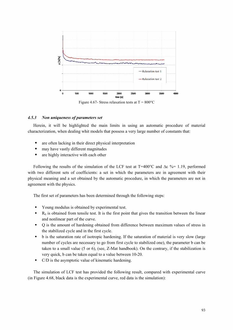
93

Figure 4.67- Stress relaxation tests at T = 800°C

4.5.3 Non uniqueness of parameters set

Herein, it will be highlighted the main limits in using an automatic procedure of material

characterization, when dealing whit models that possess a very large number of constants that:

are often lacking in their direct physical interpretation

may have vastly different magnitudes

are highly interactive with each other

Following the results of the simulation of the LCF test at T=400°C and %= 1.19, performed

with two different sets of coefficients: a set in which the parameters are in agreement with their

physical meaning and a set obtained by the automatic procedure, in which the parameters are not in

agreement with the physics.

The first set of parameters has been determined through the following steps:

Young modulus is obtained by experimental test.

R0 is obtained from tensile test. It is the first point that gives the transition between the linear

and nonlinear part of the curve.

Q is the amount of hardening obtained from difference between maximum values of stress in

the stabilized cycle and in the first cycle.

b is the saturation rate of isotropic hardening. If the saturation of material is very slow (large

number of cycles are necessary to go from first cycle to stabilized one), the parameter b can be

taken to a small value (5 or 6), (see, Z-Mat handbook). On the contrary, if the stabilization is

very quick, b can be taken equal to a value between 10-20.

C/D is the asymptotic value of kinematic hardening.

The simulation of LCF test has provided the following result, compared with experimental curve

(in Figure 4.68, black data is the experimental curve, red data is the simulation):

94

Figure 4.68- LCF test at T=400°C and %= 1.19 - Comparison between simulated and experimental test

The comparison shows a good agreement between material response and experimental data.

The second set of parameters was determined by the automatic procedure of identification, through

simulations and optimizations performed with Z-Sim and Z-Opt modules. The simulation of the same

LCF test provided the following result:

Figure 4.69- LCF test at T=400°C and %= 1.19 - Comparison between simulated and experimental test

Again, the comparison shows a good agreement between material response and experimental data,

even if, in this case, some parameters are lacking in their direct physical interpretation and have

different order of magnitude (compared to the previous set).

95

In fact, passing from the first to the second set, the initial yield stress, in the model R0 coefficient,

dropped from R0 = 400 to R0 = 101, while the asymptotic value of kinematic hardening C/D increased

by C/D = 140 to C/D = 440.

The automatic procedure is based on a mathematical optimization and not always, the results are in

agreement with the physics.

It is still possible to observe by the comparison between experimental curve (black data) and

simulation (red data) in Figure 4.69, that even if the model shows a good predictive capability, it is not

able to model correctly the yield stress.

Moreover, this result shows that the set of parameter obtained through the optimization procedure

may not be unique.

The reason is that the optimization code works for obtaining the "best fit" between the curves.

When the number of parameters is very high, this kind of optimization gives in output a result that

may be correct by a mathematical point of view, but far from the real physical meaning of coefficients.

In this case, only a good experimental database with a consistent number of tests may limit the

uncertainties.

To design an experimental database that respects these conditions is the real issue for a correct

characterization of material.

4.5.4 Sensitivity of the model to the single parameters (E, R0)

Here, it has been analysed which parameters influence mainly the material model response.

It has already shown that material model is very sensitive to Young Modulus parameter.

A little variation in Young modulus can change significantly the correspondence between model

response and experimental data.

Another parameter that affects significantly the model response is R0. Then, see how model response

changes varying only R0 parameter.

Following, the simulation of a LCF test (total strain range %19.1 , T=400°):

96

-0,008 -0,006 -0,004 -0,002 0,000 0,002 0,004 0,006 0,008

epsilon [mm/mm]

sig

ma

[Mpa]

Experimental test

Simulated test

Figure 4.70- LCF test at T=400°C and %= 1.19 - Comparison between simulated and experimental test

Changing in the model only R0 parameter (in particular, being the initial yield stress, its real value

was chosen) the result was:

-0,008 -0,006 -0,004 -0,002 0,000 0,002 0,004 0,006 0,008

epsilon [mm/mm]

sig

ma

[Mp

a]

Simulated test

Experimental test

Figure 4.71- LCF test at T= 400°C and %= 1.19 - Comparison between simulated and experimental test,changing R0

As previously observed, this anomalous response of the model depends by the optimization

process, since it performs a best fit between experimental data and simulated curve (the process is an

iterative loop for minimizing the error). Again, it has been shown that the final result often give

parameters that are missing in their real physical meaning.

Besides, the sensitivity of the model response to the coefficient R0 has been here highlighted.

An error in its evaluation involves a significant error in the predictive response of material

behaviour.

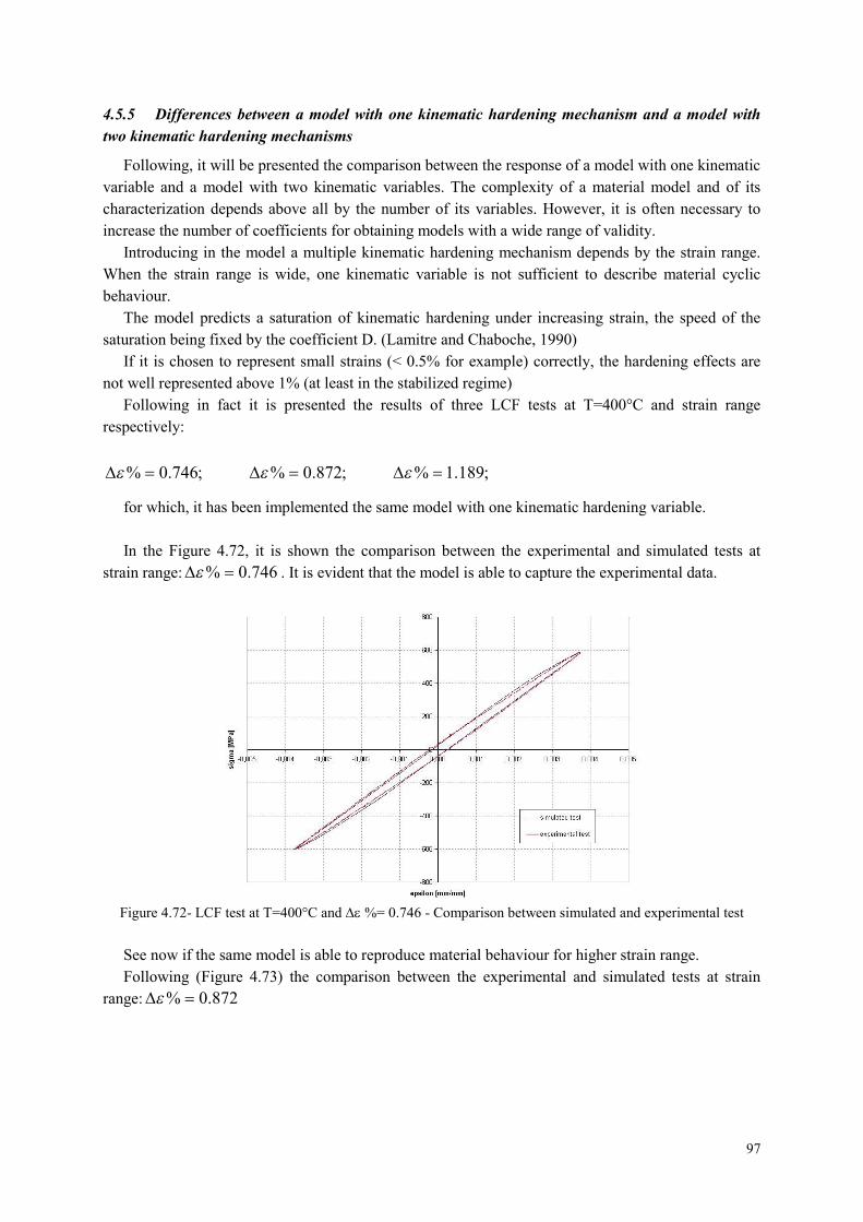
97

4.5.5 Differences between a model with one kinematic hardening mechanism and a model with

two kinematic hardening mechanisms

Following, it will be presented the comparison between the response of a model with one kinematic

variable and a model with two kinematic variables. The complexity of a material model and of its

characterization depends above all by the number of its variables. However, it is often necessary to

increase the number of coefficients for obtaining models with a wide range of validity.

Introducing in the model a multiple kinematic hardening mechanism depends by the strain range.

When the strain range is wide, one kinematic variable is not sufficient to describe material cyclic

behaviour.

The model predicts a saturation of kinematic hardening under increasing strain, the speed of the

saturation being fixed by the coefficient D. (Lamitre and Chaboche, 1990)

If it is chosen to represent small strains (< 0.5% for example) correctly, the hardening effects are

not well represented above 1% (at least in the stabilized regime)

Following in fact it is presented the results of three LCF tests at T=400°C and strain range

respectively:

;746.0% ;872.0% ;189.1%

for which, it has been implemented the same model with one kinematic hardening variable.

In the Figure 4.72, it is shown the comparison between the experimental and simulated tests at

strain range: 746.0% . It is evident that the model is able to capture the experimental data.

Figure 4.72- LCF test at T=400°C and %= 0.746 - Comparison between simulated and experimental test

See now if the same model is able to reproduce material behaviour for higher strain range.

Following (Figure 4.73) the comparison between the experimental and simulated tests at strain

range: 872.0%

98

Figure 4.73- LCF test at T= 400°C and %= 0.872 - Comparison between simulated and experimental test

It is already evident how at the increasing of the strain range, the model is anymore able to describe

material behaviour.

Again, performing a LCF test in which the strain range is: 189.1% , the comparison between

experimental data and simulated one shows a bad predictive capability of the model (Figure 4.74)

Figure 4.74- LCF test at T= 400°C and %= 1.189 - Comparison between simulated and experimental test

The same comparison, shown in Figure 4.74, was repeated and the result is shown in Figure 4.75.

In this case, the test was simulated adding to the material model a second kinematic hardening

mechanism. The first kinematic variable saturates quickly and models accurately the linear behaviour.

The second variable works for higher strains and models accurately the transition and the non-linear

behaviour. By the comparison with the experimental curve, it is evident how increasing the number of

parameters has allowed to obtain a better model response.

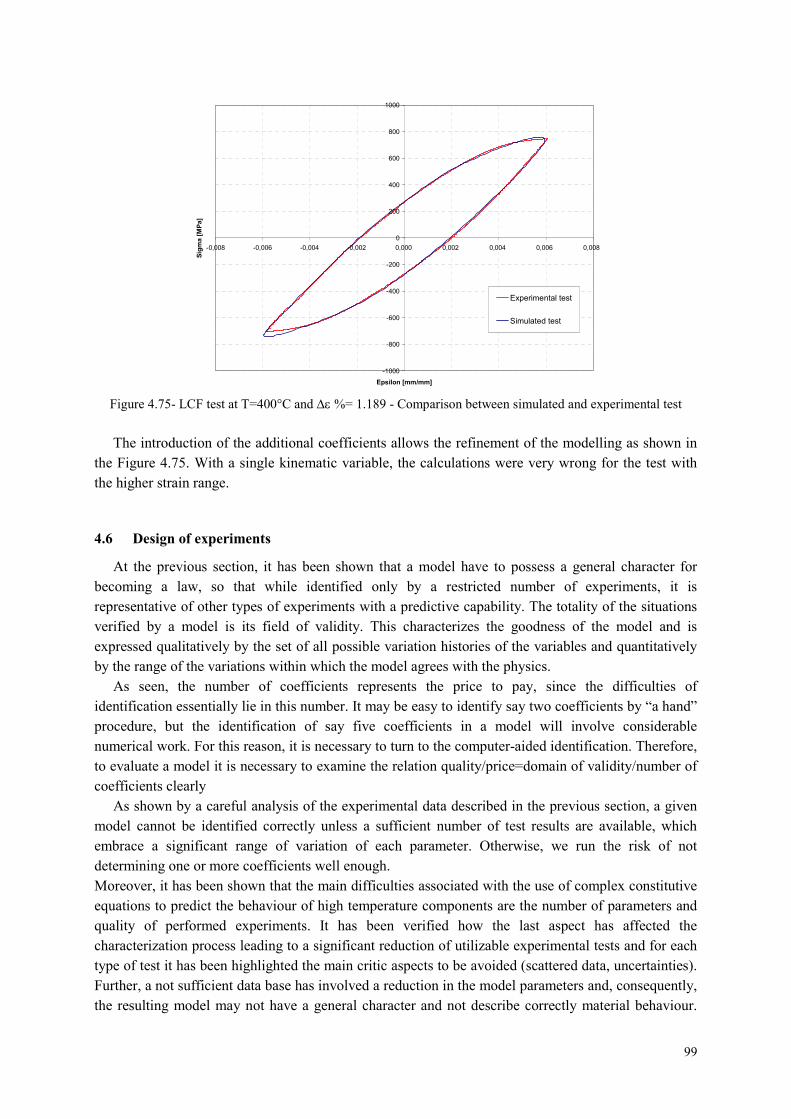
99

-1000

-800

-600

-400

-200

0

200

400

600

800

1000

-0,008 -0,006 -0,004 -0,002 0,000 0,002 0,004 0,006 0,008

Epsilon [mm/mm]

Sig

ma

[MP

a]

Experimental test

Simulated test

Figure 4.75- LCF test at T=400°C and %= 1.189 - Comparison between simulated and experimental test

The introduction of the additional coefficients allows the refinement of the modelling as shown in

the Figure 4.75. With a single kinematic variable, the calculations were very wrong for the test with

the higher strain range.

4.6 Design of experiments

At the previous section, it has been shown that a model have to possess a general character for

becoming a law, so that while identified only by a restricted number of experiments, it is

representative of other types of experiments with a predictive capability. The totality of the situations

verified by a model is its field of validity. This characterizes the goodness of the model and is

expressed qualitatively by the set of all possible variation histories of the variables and quantitatively

by the range of the variations within which the model agrees with the physics.

As seen, the number of coefficients represents the price to pay, since the difficulties of

identification essentially lie in this number. It may be easy to identify say two coefficients by “a hand”

procedure, but the identification of say five coefficients in a model will involve considerable

numerical work. For this reason, it is necessary to turn to the computer-aided identification. Therefore,

to evaluate a model it is necessary to examine the relation quality/price=domain of validity/number of

coefficients clearly

As shown by a careful analysis of the experimental data described in the previous section, a given

model cannot be identified correctly unless a sufficient number of test results are available, which

embrace a significant range of variation of each parameter. Otherwise, we run the risk of not

determining one or more coefficients well enough.

Moreover, it has been shown that the main difficulties associated with the use of complex constitutive

equations to predict the behaviour of high temperature components are the number of parameters and

quality of performed experiments. It has been verified how the last aspect has affected the

characterization process leading to a significant reduction of utilizable experimental tests and for each

type of test it has been highlighted the main critic aspects to be avoided (scattered data, uncertainties).

Further, a not sufficient data base has involved a reduction in the model parameters and, consequently,

the resulting model may not have a general character and not describe correctly material behaviour.

100

For this reason, it wants to provide guidelines for designing experiments able to identify the optimal

set of parameters.

It is necessary to fit the material properties and behaviour to be investigated. The developed work

has led to identify the constitutive equations able to predict the behaviour of high temperature

components under cyclic loads.

It has been shown that two dissipation potentials, which describe the evolution mechanisms of

inelastic deformation associated respectively to slow and high strain rates, are necessary to accurately

capture the loading-rate dependency of material behaviour. Besides, it has been show how in the case

of cyclic loading, a multiple hardening mechanism does a significantly better job of representing the

real material behaviour over the entire strain range. In order to describe the evolution of the hardening

under cyclic loads, the combination of isotropic and kinematic models has been implemented, in this

way it has been modelled the size variation of elastic domain and of its translation. The viscoplasticity

with isotropic and kinematic hardening combine plasticity and creep and allow taking into account of

the rate dependence.

The identification of the constitutive laws, able to describe the material behaviour, provides a

reference for a correct designing of experimental tests.

The data have to be quite extensive, a sufficient number of repetitions for each test have to be

provided, as well as a sufficient variety of experimental data in order to obtain a model with a general

character and a wide field of validity. Besides, two different groups of tests have to be designed: for

characterization and validation processes respectively. In particular, tests within the reversible domain

(i.e., creep with recovery upon complete unloading, and relaxation) and experiments conducted within

the irreversible domain (i.e., relaxation, conventional creep, multi-step creep, tensile curves at

different total strain rates) have to be used for characterization; while multiple-step relaxation, cyclic

and plasticity/creep interaction tests have to be reserved for validating the predictive behaviour of the

model.

It is important to realize from the outset, that the resulting set of material parameters is non-unique

(due to the non-linear nature of the problem), however if a sufficient amount of “data content” is

available, then it believes that the final obtained parameters are relatively independent of the initial

guess and bounds provided.

It is suggested to separate the characterization process of the elasto-visco-plastic model in more

stages:

1) Determine the viscous flow and initial yield stress (n, k, R0) using the tensile curves at different

total strain rates. This kind of tests allows calibrating the viscous effects and the dependence of

material behaviour by loading - rate.

2) Determine the hardening parameters (C, D, Q, b) by the LCF tests and LCF-step tests. The

implementation of the non-linear kinematic hardening model allows taking into account of the effects

due to the deformation history by determining the increment of accumulated plastic strain. This allow

considering a hardening varying with continuity for describing the non-linearity of the process of

cyclic plastic deformation.

3) Determine the thermal recovery parameters (m, M) given the relaxation, conventional creep and

multi-step creep tests while keeping the flow and hardening parameter estimates from step 1 and 2

fixed. These kinds of tests allow describing the time-dependent (short-term and long-term) material

behaviour.

4) Fit all tests at one time to obtain final parameter estimates, this is accomplished by allowing all

visco-plastic parameters to be active (using the material parameters found in steps 1, 2 and 3 as initial

starting values) but with tight upper and lower bounds around each parameter.

101

This approach allows reducing the convergence problems of solution described previously.

In the designing of experimental tests, it is important to consider that if one focused on only one

type of loading condition, superior correlations could of course be achieved for that class of loading.

However, predictions of other classes of loading may severely suffer. For example, during a separate

characterization process involving only tensile tests, excellent correlation was obtained, but at the

expense of poor creep and relaxation behaviour for a given set of material parameters. Conversely,

when the model was calibrated for creep responses, poorer tensile and relaxation behaviours were

similarly predicted. Thus when judging the “goodness” of a given model, one must keep in mind the

appropriate required “data content” for accurately capturing the full range of material behaviour of

interest.

For an identical material and model, it may be necessary to define several sets of coefficients, each

better suited to a domain of variation or to a load type, for example, rapid transient loads, short-term

loads, long-term loads and stationary loads.

Another important aspect is the scattering of experimental results. This can be due to:

The nature of the phenomenon, inhomogeneities, random growth processes, and load

uncertainty.

The inherent scattering in each sample arising from the production or casting process

and also from the heat treatment, and so on.

Usually, scattering is of the order of 1-5% for elastic strains, 10-50% for plastic or viscoplastic

strains, 50-100% (factor of 2) of the number of cycles for low cycle fatigue crack initiation or growth,

and 1000% (factor of 10) for fatigue failure in the high cycle regime.

These orders of magnitude of scattering indicate at once the pronounced influence of nonlinearities

of the phenomena. The simplest and most efficient way of including this scattering in a model consists

in giving a statistical definition to the multiplying coefficients present in the model. (Lemaitre and

Chaboche, 1990)

Knowing a mathematical model by its analytical expression, and obtaining a set of experimental

results in which all the variables of the model have been activated, one is in a position to calculate the

unknown coefficients that give the best representation of the experimental results.

4.6.1 Check by phenomenological aspect

At the end of the identification process of material model parameters, it is necessary to make a

check through the evaluation of phenomenological aspects derived experimentally.

As described in the previous section, useful information, to perform a procedure of material

characterization, are provided by the identification of the stabilized cyclic hardening curve, i.e., the

peaks of stabilized cycles (max, p,max) in the (, p) graph.

Cyclic hardening curve can be located above (cyclic hardening) or below (cyclic softening) the

monotonic hardening curve. The identification of its expression in terms of stress and strain variables

presents a problem linked to the history of deformation. As a matter of fact, the curve may not be

exactly the same if it is obtained by continuous variation, as it would be if it is obtained by imposing

finite increments in stress or strain ranges, or if one or several specimens are used.

To identify a simple relation between the stress and strain ranges and to verify the uniqueness of

the cyclic hardening curve, several methods can be used.

It is recommended of performing tests in which the strains are varied stepwise, first increasing and

then decreasing. After stabilization of hardening at the lowest level, a resumption of hardening at a

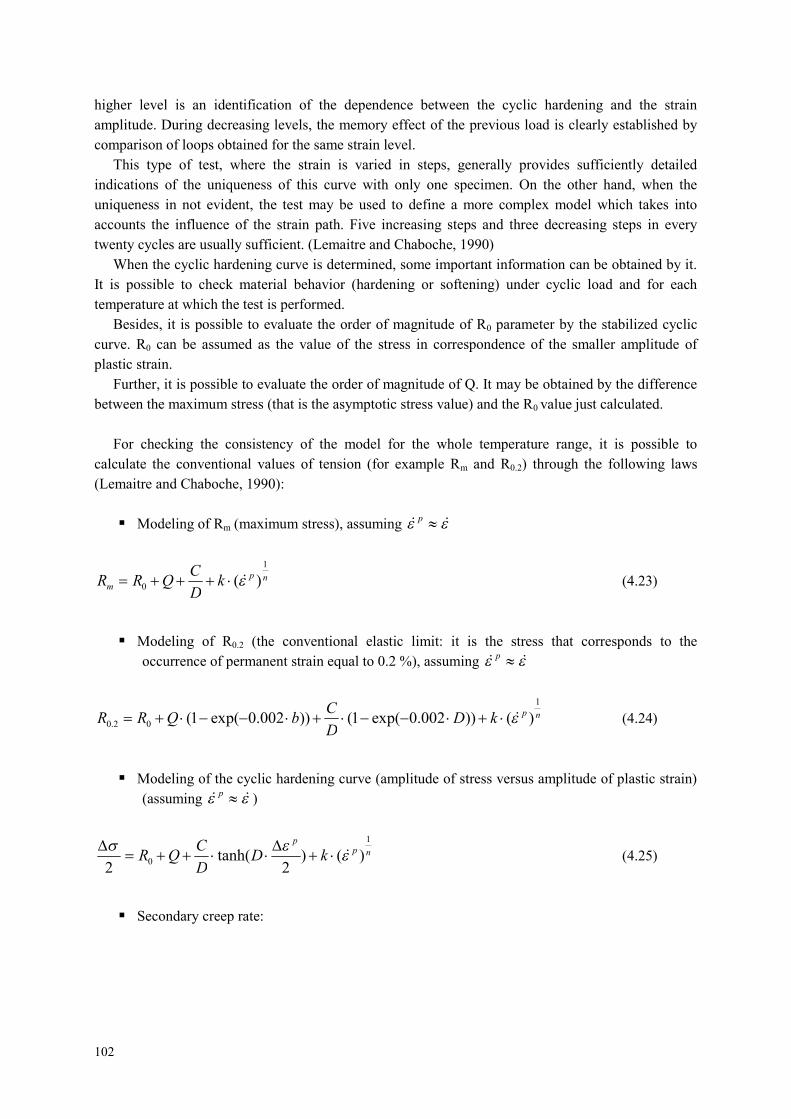
102

higher level is an identification of the dependence between the cyclic hardening and the strain

amplitude. During decreasing levels, the memory effect of the previous load is clearly established by

comparison of loops obtained for the same strain level.

This type of test, where the strain is varied in steps, generally provides sufficiently detailed

indications of the uniqueness of this curve with only one specimen. On the other hand, when the

uniqueness in not evident, the test may be used to define a more complex model which takes into

accounts the influence of the strain path. Five increasing steps and three decreasing steps in every

twenty cycles are usually sufficient. (Lemaitre and Chaboche, 1990)

When the cyclic hardening curve is determined, some important information can be obtained by it.

It is possible to check material behavior (hardening or softening) under cyclic load and for each

temperature at which the test is performed.

Besides, it is possible to evaluate the order of magnitude of R0 parameter by the stabilized cyclic

curve. R0 can be assumed as the value of the stress in correspondence of the smaller amplitude of

plastic strain.

Further, it is possible to evaluate the order of magnitude of Q. It may be obtained by the difference

between the maximum stress (that is the asymptotic stress value) and the R0 value just calculated.

For checking the consistency of the model for the whole temperature range, it is possible to

calculate the conventional values of tension (for example Rm and R0.2) through the following laws

(Lemaitre and Chaboche, 1990):

Modeling of Rm (maximum stress), assuming p

npm k

D

CQRR

1

0 )( (4.23)

Modeling of R0.2 (the conventional elastic limit: it is the stress that corresponds to the

occurrence of permanent strain equal to 0.2 %), assuming p

npkDD

CbQRR

1

02.0 )())002.0exp(1())002.0exp(1( (4.24)

Modeling of the cyclic hardening curve (amplitude of stress versus amplitude of plastic strain)

(assuming p )

npp

kDD

CQR

1

0 )()2

tanh(2

(4.25)

Secondary creep rate:

103

n

p

k

RRD

C0

(4.26)

Asymptotic stress in relaxation:

D

CQR 0 (4.27)

In this way it is possible to verify the goodness of the coefficients set by the phenomenological

aspects determined experimentally.

As a matter of fact, the known parameters ( ,,, 2.0p

m RR , cyclic hardening curve) obtained in

output from experimental tests, may be calculated according the previous equations (that involve the

model coefficients), and by the comparison between the order of magnitude of the values such

calculated and their real values, it is possible to verify preliminarily the coefficients set.

At the end, the order of magnitude of the coefficient k may be also verified by the Norton law:

nv k

1

)( (4.28)

In which v is viscous stress. The difference between the tensile tests at different strain rates

allows evaluating the amplitude of the viscous stress and by the previous equation, it is possible to

calculate k value for one strain rate (supposing a fixed value for n).

104

5 Application of elasto-visco-plastic material models to cases of industrialinterest.

5.1 Introduction

In the present chapter, it will be described in which way a procedure for FEM structural analysis,

implementing elasto-visco-plastic material models, has been developed and validate, in order to

determine stress-strain state of components under cyclic loads and high temperatures.

Elasto-visco-plastic analysis allows evaluating the real material behaviour and structure life in a

more accurate way, taking into account the nonlinear interaction between the two mechanisms of

damage: fatigue and creep.

In particular, starting from an elasto-visco-plastic material model, already characterized and

validated, it has been possible to test its effectiveness by performing comparison analysis with known

models in linear-elastic and elasto-plastic fields.

Besides, by the implementation of known damage models a procedure for calculating structure life

taking into account of nonlinear interaction between creep and fatigue has been developed and validate

The methodology of analysis has been applied to a case of industrial interest. An elasto-visco-

plastic analysis has been performed on a combustion chamber of aeronautical engine and structure life

has been evaluated.

Finally, the response of material model, characterized at the previous chapter, has been evaluated.

The model has been implemented to perform a preliminary elasto-visco-plastic analysis on a portion of

a turbine blade.

Starting from the obtained results, it will be possible to plan a new campaign of experimental tests

for a complete material characterization.

The introduction of such complex models will allow an improvement of turbine blades designing.

In fact, the capability of reproducing the real material behaviour and predicting the component life in a

more accurate way, allow reducing the traditional factors of safety that are overly conservative and

preventing from achieving the optimal efficiency in structural designing process.

5.2 Procedure of elasto-visco-plastic analysis

The objective of this section is to develop a procedure of structural analysis that, through the

comparison with procedures of tested validity, allows a correct and safe implementation of elasto-

visco-plastic material models.

The comparison between structural analysis of a component modeled to finite elements using

ANSYS standard material models and user-defined material models implemented in ANSYS through

the interface with Z-Mat code, has been developed through the following phases:

Choice of a test case

Linear elastic analysis

Elasto-plastic analysis

105

Elasto-visco-plastic analysis

The activities that will be described in the present section have been developed in collaboration

with AVIO-Propulsione Aerospaziale.

Elasto-Visco-Plastic analysis can be performed adopting Z-Ansys module implemented in Z-Mat

software. It is sufficient to generate a subroutine that links ANSYS to Z-Mat. More in detail will be

sufficient to put in a folder

The file (i.e. Jobname.inp) containing FE model, loads, boundary conditions and solution

parameters.

The file containing all the necessary material parameters (classes, modules and

coefficients).

It is important to notice that the material filename must be always defined as 10x.txt where x is a

number varying from 1 to 9. If there will be different materials constituting the structural component,

it will be necessary to insert different files for each material.

The first step is to choose the ANSYS elements that are defined as user-mat; in fact, for these kinds

of elements will be possible to define an external material model and behaviour.

The file jobname.inp is obtained by issuing the ANSYS command CDWRITE after than the model

has been completely meshed, all the boundary conditions and forces have been applied, and a dummy

material model has been assigned.

In the /PREP7 section, after the ANTYPE command, which selects the type of analysis, must be

added the lines recalling the external material model. Using the TB Ansys command with the USER

and STATE options:

TB, USER, 1, 0, 0

TB, STATE, , 40

These lines recall the material file defined as 101.txt

At the end of all these activities, the /SOLU Ansys command must be issued. In this step must be

defined the type of analysis and its options, loads will be applied, together with load-step options.

Through the EQSLV is chosen the type of analysis. The preferred one must be the PCG (Pre-

conditioned Conjugate Gradient iterative equation solver), because is the one that best fits non-linear

analyses.

Issuing the command NROPT,FULL,,OFF “complete” Newton-Raphson method will be selected,

in this way, the stiffness matrix of the element is calculated at each equilibrium iteration. At this

command, has been associated the option adaptive descent off that uses “tangent stiffness matrix”

every equilibrium iteration.

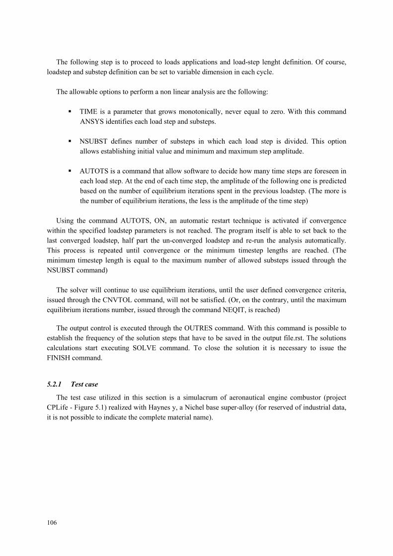
106

The following step is to proceed to loads applications and load-step lenght definition. Of course,

loadstep and substep definition can be set to variable dimension in each cycle.

The allowable options to perform a non linear analysis are the following:

TIME is a parameter that grows monotonically, never equal to zero. With this command

ANSYS identifies each load step and substeps.

NSUBST defines number of substeps in which each load step is divided. This option

allows establishing initial value and minimum and maximum step amplitude.

AUTOTS is a command that allow software to decide how many time steps are foreseen in

each load step. At the end of each time step, the amplitude of the following one is predicted

based on the number of equilibrium iterations spent in the previous loadstep. (The more is

the number of equilibrium iterations, the less is the amplitude of the time step)

Using the command AUTOTS, ON, an automatic restart technique is activated if convergence

within the specified loadstep parameters is not reached. The program itself is able to set back to the

last converged loadstep, half part the un-converged loadstep and re-run the analysis automatically.

This process is repeated until convergence or the minimum timestep lengths are reached. (The

minimum timestep length is equal to the maximum number of allowed substeps issued through the

NSUBST command)

The solver will continue to use equilibrium iterations, until the user defined convergence criteria,

issued through the CNVTOL command, will not be satisfied. (Or, on the contrary, until the maximum

equilibrium iterations number, issued through the command NEQIT, is reached)

The output control is executed through the OUTRES command. With this command is possible to

establish the frequency of the solution steps that have to be saved in the output file.rst. The solutions

calculations start executing SOLVE command. To close the solution it is necessary to issue the

FINISH command.

5.2.1 Test case

The test case utilized in this section is a simulacrum of aeronautical engine combustor (project

CPLife - Figure 5.1) realized with Haynes y, a Nichel base super-alloy (for reserved of industrial data,

it is not possible to indicate the complete material name).

107

Figure 5.1- Simulacrum of CPLife combustor

In Figure 5.2 and Figure 5.3, it is shown respectively the geometry of simulacrum and a particular

of the ring holding. The simulacrum, in fact, is divided in two parts: liner and ring holding.

Figure 5.2- Simulacrum geometry

Figure 5.3- Ring holding

The FEM model of simulacrum has been realized (Figure 5.4). The element type is SOLID186 and

the model details are summarized in Table 5.1.

NODES ELEMENTS

TOTAL MODEL 56005 10061

LINER 47829 8736

RING HOLDING 8176 1325

Table 5.1 – FEM model details

108

Figure 5.4- FEM model

The mechanical loads are the difference of pressure between internal and external face of the liner

p = 0.018 MPa and the closing pressure on the ring p = 0.0509 MPa (Figure 5.5).

Figure 5.5- Simulacrum FEM model - Mechanical loads

The constraints are applied on nodes located in front section of liner to block axial and tangential

displacements (Figure 5.6).

Figure 5.6- Simulacrum FEM model - Constraints

The thermal maps applied to the model were determined through experimental measurements. In

Figure 5.7, it is shown the thermal loads in the maximum stabilized condition in service.

109

Figure 5.7- Simulacrum FEM model – Thermal loads (plane development)

Loads, constraints and material data were obtained by CPLife documentation, made available by

AVIO.

5.2.2 Linear-elastic analysis

By the available material experimental data (CPLife documentation) and by the methodology of

material characterization developed and described at the previous chapter, a linear-elastic material

model has been developed and implemented in ANSYS code through the software Z-Mat. In this way,

a linear analysis has been performed on simulacrum.

To verify the reliability of the developed material model and its correct implementation in ANSYS,

an analogous analysis has been performed utilizing the linear-elastic model of FEM code.

Figure 5.8- Linear-elastic analysis - Von Mises stress – plane development

In Figure 5.8 it is shown the comparison between the results of the two analysis. In particular, on

the left the Von Mises stress (plane development) obtained from the analysis performed utilizing the

ANSYS (v 10.0) linear-elastic material model. On the right, the Von Mises stress (plane development)

obtained from the analysis performed implementing the external defined material in ANSYS (v 6.1).

By the comparison, the stress analysis has provided values with a gap not higher than 1.2 %. With

the exception of the most critical zone of the dilution hole where, in correspondence of the peaks, the

gap does not exceed the 11.1% (Figure 5.9 and Figure 5.10).

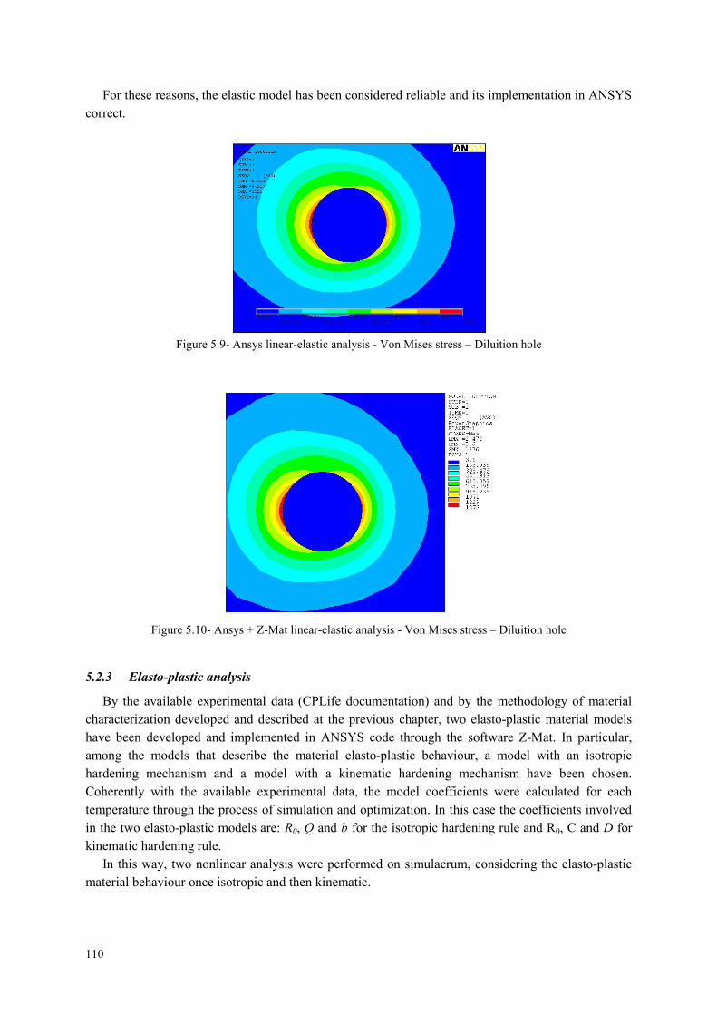
110

For these reasons, the elastic model has been considered reliable and its implementation in ANSYS

correct.

Figure 5.9- Ansys linear-elastic analysis - Von Mises stress – Diluition hole

Figure 5.10- Ansys + Z-Mat linear-elastic analysis - Von Mises stress – Diluition hole

5.2.3 Elasto-plastic analysis

By the available experimental data (CPLife documentation) and by the methodology of material

characterization developed and described at the previous chapter, two elasto-plastic material models

have been developed and implemented in ANSYS code through the software Z-Mat. In particular,

among the models that describe the material elasto-plastic behaviour, a model with an isotropic

hardening mechanism and a model with a kinematic hardening mechanism have been chosen.

Coherently with the available experimental data, the model coefficients were calculated for each

temperature through the process of simulation and optimization. In this case the coefficients involved

in the two elasto-plastic models are: R0, Q and b for the isotropic hardening rule and R0, C and D for

kinematic hardening rule.

In this way, two nonlinear analysis were performed on simulacrum, considering the elasto-plastic

material behaviour once isotropic and then kinematic.

111

To verify the reliability of the developed material models and their correct implementation in

ANSYS, the same experimental data were utilized for defining the elasto-plastic material models

already available in ANSYS library.

In particular, the ANSYS elasto-plastic material models with isotropic and kinematic hardening are

respectively: MISO (Multilinear Isotropic Hardening) and MKIN (Multinilear Kinematic Hardening).

Besides, these are the material models utilized for this type of structural analysis, until now.

Multilinear Kinematic Hardening option (MKIN) uses the Besseling model, also called the sub-

layer or overlay model. Heterogeneous nature of deformations causes, in microscopic scale, a network

of dislocations in directions imposed by load type. In this way, hardening is not uniform in all

directions (Bauschinger effect), see Figure 5.11.

Figure 5.11- Multilinear kinematic hardening rule- Bauschinger effect

In this model, the material is seen as a set of sub-layers. The plastic strains remain constant by

scaling the sub-layers. Each sub-layer is characterized by a simple stress-strain curve and, by

combining these curves, the multilinear response is obtained (Figure 5.12), that shows the effect of

kinematic hardening.

Figure 5.12 – Multilinear kinematic response

With the command MKIN is possible to introduce the stress-strain curves for temperature

dependent properties.

112

Figure 5.13- Multilinear kinematic hardening -curves

In Figure 5.13, an example of typical stress-strain curves for the MKIN option, where each of them

is a stress-strain curve (obtained by five stress-strain values) at constant temperature.

Multilinear Isotropic Hardening option (MISO) uses Von Mises Yield criterion. Deformations

cause accumulation of intermolecular dislocations. This causes material hardening, because of the

dislocations obstruct motion among crystalline planes. Hardening rule is assumed uniform in all load

directions (Figure 5.14).

Figure 5.14- Multilinear isotropic hardening rule

The multilinear isotropic hardening response is shown in Figure 5.15:

Figure 5.15 – Multilinear isotropic response

With the command MISO is possible to introduce the stress-strain curves for temperature

dependent properties, so, for each temperature, multilinear stress-strain curves are implemented. The

113

MISO option can contain up to twenty different temperature curves, with up to one hundred different

stress-strain points allowed per curve.

The experimental stress-strain curves implemented in ANSYS for both options MKIN and MISO

are the following (defined in the temperature range of the analysis), see Figure 5.16:

Figure 5.16 – Curve MKIN – MISO for simulacrum material model definition in ANSYS

In this way, two elasto-plastic analysis analogous to the ones performed implementing external

material models, have been executed.

Following, the comparisons between the analysis performed implementing external material

models and ANSYS elasto-plastic models.

The first comparisons refer to the analysis performed considering elasto-plastic material behaviour

with isotropic hardening.

In Figure 5.17, it is shown the comparison between the Von Mises stress calculated with ANSYS

material model (MISO) (on the left) and implementing in ANSYS the Z-Mat elasto-plastic material

model with isotropic hardening (on the right).

Figure 5.17 – Elasto-plastic analysis (isotropic hardening) - Von Mises stress

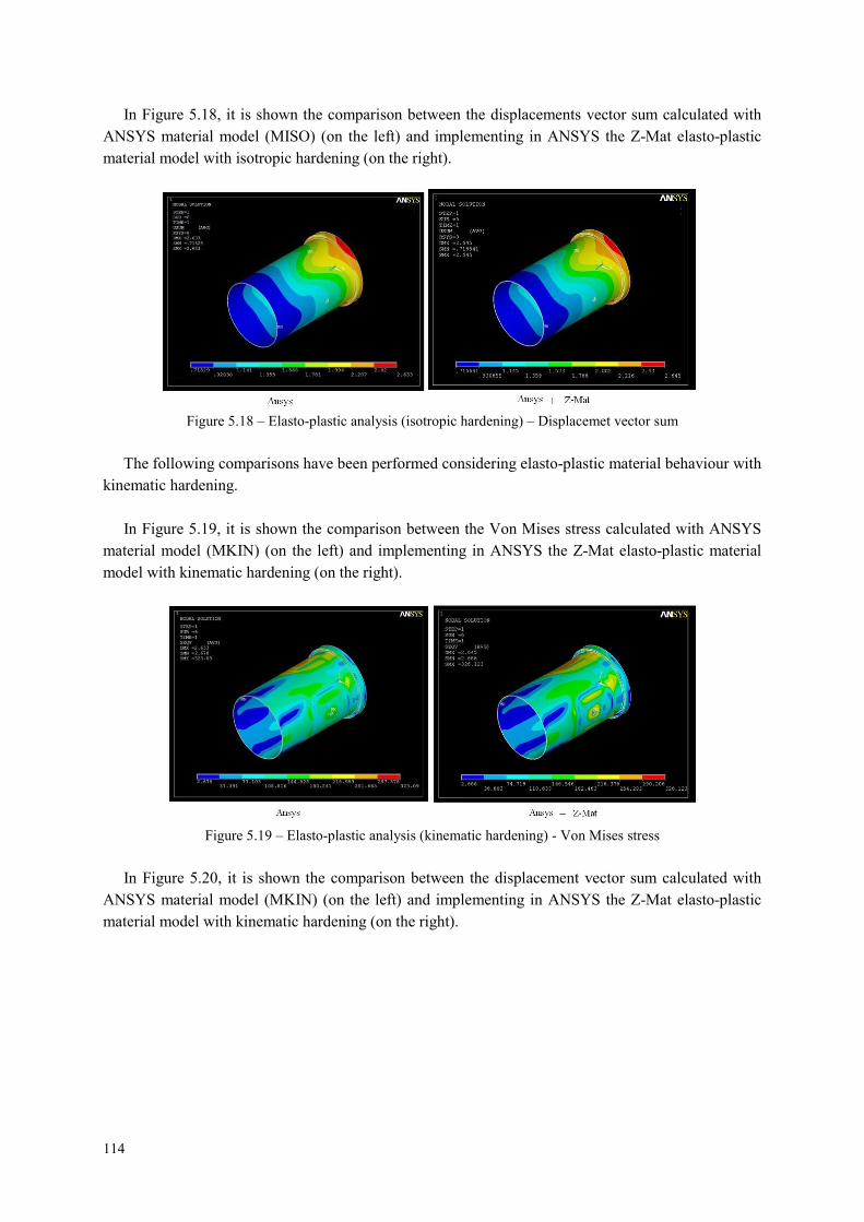
114

In Figure 5.18, it is shown the comparison between the displacements vector sum calculated with

ANSYS material model (MISO) (on the left) and implementing in ANSYS the Z-Mat elasto-plastic

material model with isotropic hardening (on the right).

Figure 5.18 – Elasto-plastic analysis (isotropic hardening) – Displacemet vector sum

The following comparisons have been performed considering elasto-plastic material behaviour with

kinematic hardening.

In Figure 5.19, it is shown the comparison between the Von Mises stress calculated with ANSYS

material model (MKIN) (on the left) and implementing in ANSYS the Z-Mat elasto-plastic material

model with kinematic hardening (on the right).

Figure 5.19 – Elasto-plastic analysis (kinematic hardening) - Von Mises stress

In Figure 5.20, it is shown the comparison between the displacement vector sum calculated with

ANSYS material model (MKIN) (on the left) and implementing in ANSYS the Z-Mat elasto-plastic

material model with kinematic hardening (on the right).

115

Figure 5.20 – Elasto-plastic analysis (kinematic hardening) – Displacemet vector sum

By the comparisons between elasto-plastic analysis performed with ANSYS material models and,

subsequently, implementing in ANSYS the developed external material models, it has been observed

in both the hypothesis of isotropic and kinematic hardening that:

The gap in displacement values is lower then 0.7 % in all considered conditions

The gap in stress values is lower then 0.93 % in all considered conditions, including the most

critical area of the dilution hole.

Since by the comparison, it has been found a good correspondence between the analysis results, it

is possible to consider correct the developed procedure of material characterization and

implementation of external material models in ANSYS.

For these reasons, the elasto-plastic models have been considered totally reliable.

5.2.4 Elasto-visco-plastic analysis

In this phase, after to have obtained the results of linear-elastic and elasto-plastic analysis, an

elasto-visco-plastic analysis has been performed on simulacrum and on specimens subjected to

characterization tests.

In this case, it was not still available all the characterization tests necessary for the development of

the Chaboche elasto-visco-plastic model of the material under examination. So, with the aim to

develop and validate a methodology of structural analysis implementing elasto-visco-plastic material

models, the Chaboche EVP model of the Nickel base superalloy Haynes x (with mechanical properties

similar to Haynes y) already characterized was utilized.

In this way, it has been evaluated the effectiveness of the elasto-visco-plastic model compared to

the results obtained by known models in linear-elastic and elasto-plastic field, previously implemented

(paragraphs 5.2.2 and 5.2.3) and until now utilized for this type of analysis.

Preliminary analysis on the specimens of tensile, LCF and creep tests, were performed in order to

test the model and its correct implementation in FEM code.

The EVP model of Haynes x was implemented in ANSYS code and numerical simulations of

characterization tests (tensile, LCF and creep) were performed. In this case, simulations of

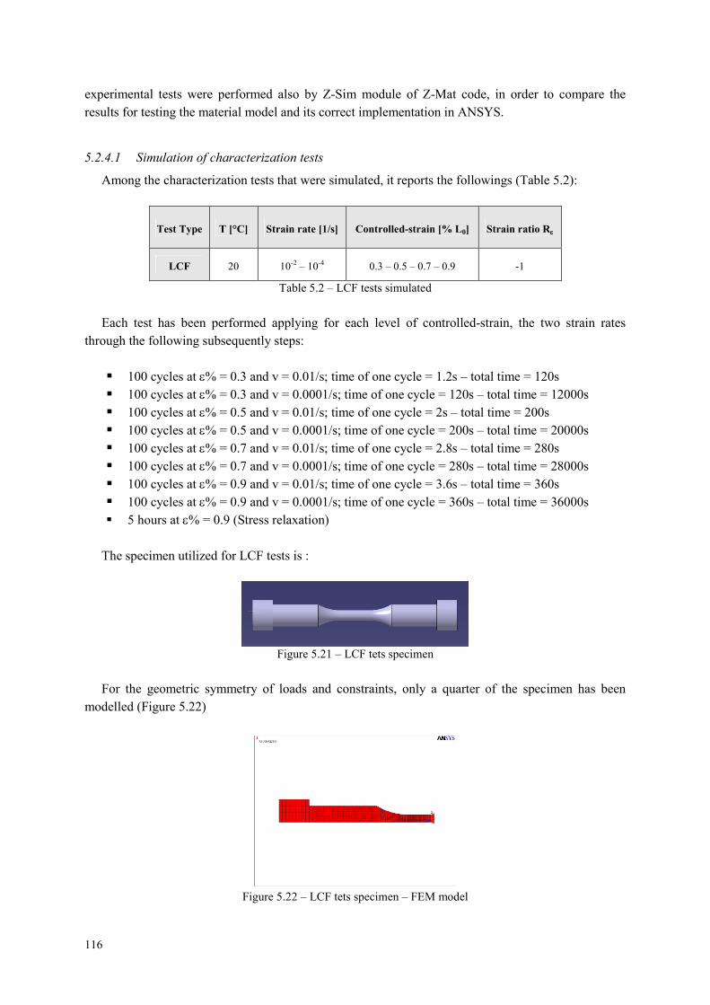
116

experimental tests were performed also by Z-Sim module of Z-Mat code, in order to compare the

results for testing the material model and its correct implementation in ANSYS.

5.2.4.1 Simulation of characterization tests

Among the characterization tests that were simulated, it reports the followings (Table 5.2):

Test Type T [°C] Strain rate [1/s] Controlled-strain [% L0] Strain ratio R

LCF 20 10-2 – 10-4 0.3 – 0.5 – 0.7 – 0.9 -1

Table 5.2 – LCF tests simulated

Each test has been performed applying for each level of controlled-strain, the two strain rates

through the following subsequently steps:

100 cycles at % = 0.3 and v = 0.01/s; time of one cycle = 1.2s – total time = 120s

100 cycles at % = 0.3 and v = 0.0001/s; time of one cycle = 120s – total time = 12000s

100 cycles at % = 0.5 and v = 0.01/s; time of one cycle = 2s – total time = 200s

100 cycles at % = 0.5 and v = 0.0001/s; time of one cycle = 200s – total time = 20000s

100 cycles at % = 0.7 and v = 0.01/s; time of one cycle = 2.8s – total time = 280s

100 cycles at % = 0.7 and v = 0.0001/s; time of one cycle = 280s – total time = 28000s

100 cycles at % = 0.9 and v = 0.01/s; time of one cycle = 3.6s – total time = 360s

100 cycles at % = 0.9 and v = 0.0001/s; time of one cycle = 360s – total time = 36000s

5 hours at % = 0.9 (Stress relaxation)

The specimen utilized for LCF tests is :

Figure 5.21 – LCF tets specimen

For the geometric symmetry of loads and constraints, only a quarter of the specimen has been

modelled (Figure 5.22)

Figure 5.22 – LCF tets specimen – FEM model

117

The main features of the FEM model are the following:

Element Type Nodes Elements

FEM Model Plane 183 2228 685Table 5.3 – Main features of FEM model

Since, it is not possible to perform controlled-strain tests in ANSYS, the displacement that causes

the controlled-strain has been calculated and applied in nodes (in correspondence of the holding area)

as shown in Figure 5.23:

Figure 5.23 – LCF tets specimen – Loads

The tests have been performed implementing the elasto-visco-plastic model of Haynes x in

ANSYS.

In Figure 5.24, it is shown the stabilized cycles obtained for each load condition.

Figure 5.24 – EVP analysis - ANSYS simulation of LCF tests at R= -1 and T=20°C (stabilized cycles)

The LCF tests, described in the Table 5.2, have been simulated through Z-Sim code applying the

same conditions and the same material model, obtaining the following results:

118

Figure 5.25 – EVP analysis – Z-Sim simulation of LCF tests at R= -1 and T=20°C

The simulations have provided the same results. In addition, simulations of experimental tensile

and creep tests have been performed both in ANSYS and Z-Sim, implementing the same material

model. Again, coincident results have been obtained. In this way, it has been possible to test the

elasto-visco-plastic material model and its correct implementation in ANSYS.

5.2.4.2 Elasto-visco-plastic analysis on combustor simulacrum

Elasto-visco-plastic analysis has been performed on simulacrum. A typical procedure of

thermomechanical stress analysis of a combustor has been applied, implementing a simpler and

cyclically repeated mission.

By comparing the results with the ones obtained from previous analysis, it has been highlighted

and verified the possibility to reproduce the physical phenomena, (for example: stress relaxation) that

may be appreciated only through an analysis performed with a rate dependent material model.

In fact, the elasto-visco-plastic model does not consider the time variable as a simple counter, that

scans the succession of load configurations, but associates to it the real physical meaning. In this way,

both the loads application and material behaviour become rate dependent.

For this reason, the material model is able to simulate at once, material creep under (thermal and

mechanical) loads for long time and the effect of “diffusion” that it causes.

The thermomechanical load cycle applied to simulacrum is shown in Figure 5.26 . The cycle

phases are:

Ignition and acceleration

Hot hold time

Cold hold time

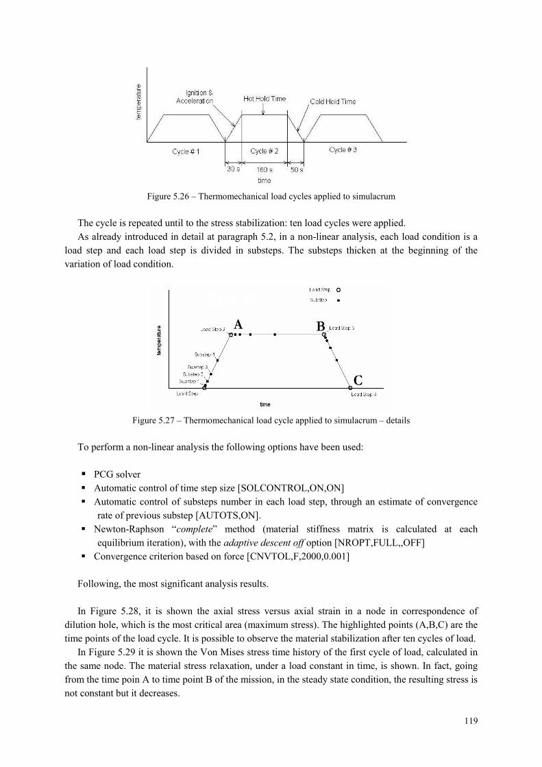
119

Figure 5.26 – Thermomechanical load cycles applied to simulacrum

The cycle is repeated until to the stress stabilization: ten load cycles were applied.

As already introduced in detail at paragraph 5.2, in a non-linear analysis, each load condition is a

load step and each load step is divided in substeps. The substeps thicken at the beginning of the

variation of load condition.

Figure 5.27 – Thermomechanical load cycle applied to simulacrum – details

To perform a non-linear analysis the following options have been used:

PCG solver

Automatic control of time step size [SOLCONTROL,ON,ON]

Automatic control of substeps number in each load step, through an estimate of convergence

rate of previous substep [AUTOTS,ON].

Newton-Raphson “complete” method (material stiffness matrix is calculated at each

equilibrium iteration), with the adaptive descent off option [NROPT,FULL,,OFF]

Convergence criterion based on force [CNVTOL,F,2000,0.001]

Following, the most significant analysis results.

In Figure 5.28, it is shown the axial stress versus axial strain in a node in correspondence of

dilution hole, which is the most critical area (maximum stress). The highlighted points (A,B,C) are the

time points of the load cycle. It is possible to observe the material stabilization after ten cycles of load.

In Figure 5.29 it is shown the Von Mises stress time history of the first cycle of load, calculated in

the same node. The material stress relaxation, under a load constant in time, is shown. In fact, going

from the time poin A to time point B of the mission, in the steady state condition, the resulting stress is

not constant but it decreases.

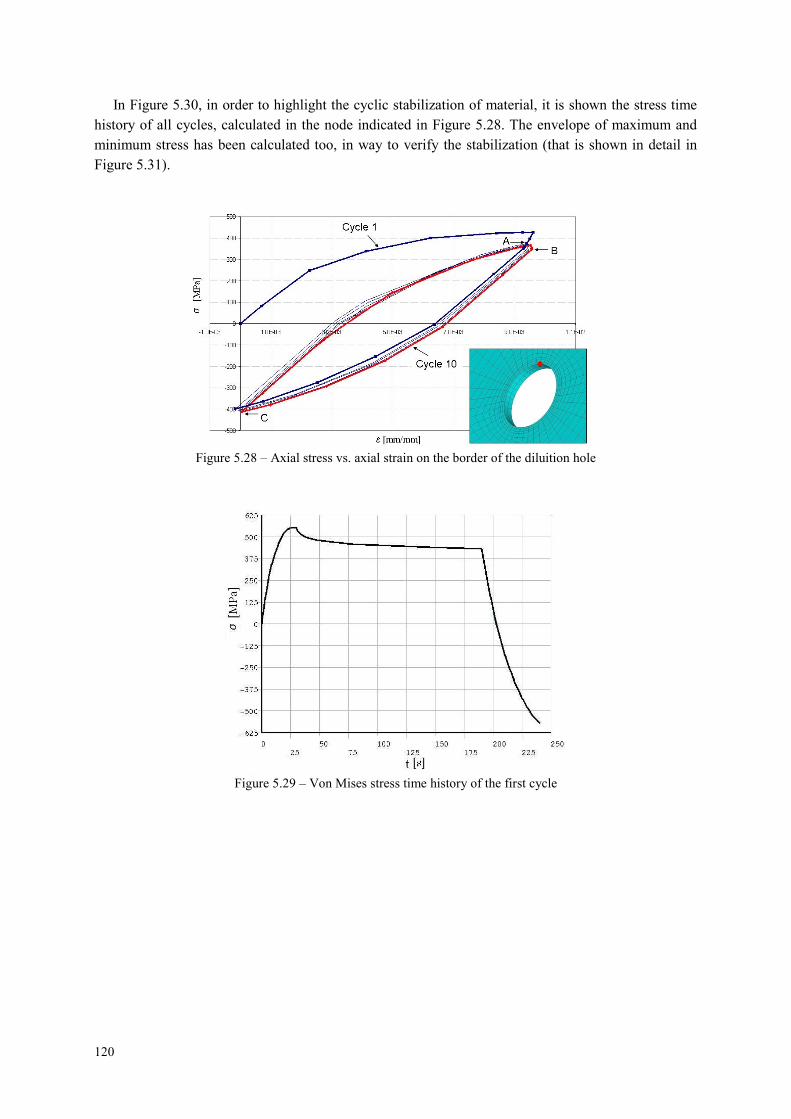
120

In Figure 5.30, in order to highlight the cyclic stabilization of material, it is shown the stress time

history of all cycles, calculated in the node indicated in Figure 5.28. The envelope of maximum and

minimum stress has been calculated too, in way to verify the stabilization (that is shown in detail in

Figure 5.31).

Figure 5.28 – Axial stress vs. axial strain on the border of the diluition hole

Figure 5.29 – Von Mises stress time history of the first cycle

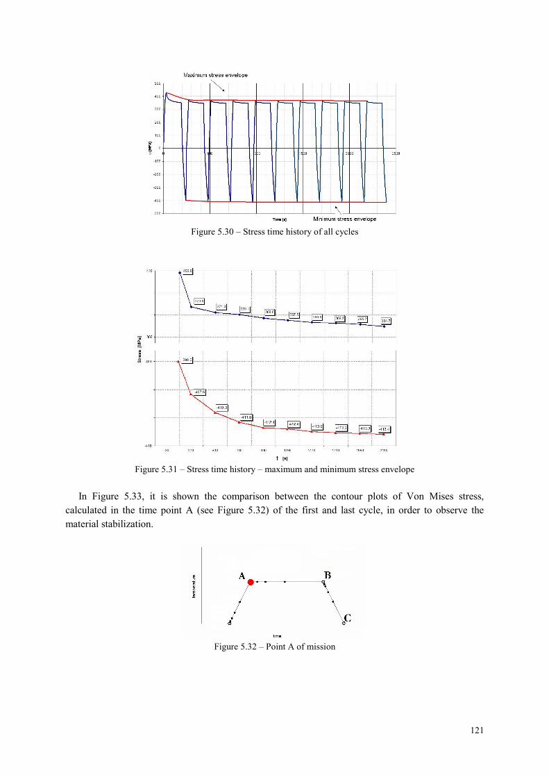
121

Figure 5.30 – Stress time history of all cycles

Figure 5.31 – Stress time history – maximum and minimum stress envelope

In Figure 5.33, it is shown the comparison between the contour plots of Von Mises stress,

calculated in the time point A (see Figure 5.32) of the first and last cycle, in order to observe the

material stabilization.

Figure 5.32 – Point A of mission

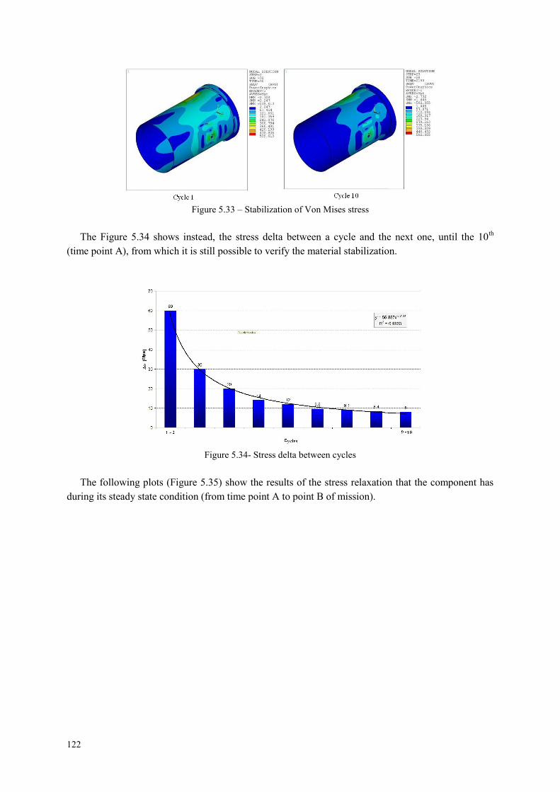
122

Figure 5.33 – Stabilization of Von Mises stress

The Figure 5.34 shows instead, the stress delta between a cycle and the next one, until the 10th

(time point A), from which it is still possible to verify the material stabilization.

Figure 5.34- Stress delta between cycles

The following plots (Figure 5.35) show the results of the stress relaxation that the component has

during its steady state condition (from time point A to point B of mission).

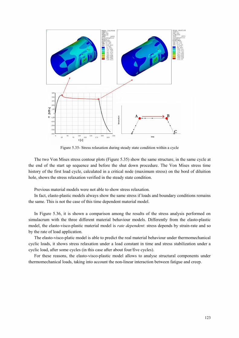
123

Figure 5.35- Stress relaxation during steady state condition within a cycle

The two Von Mises stress contour plots (Figure 5.35) show the same structure, in the same cycle at

the end of the start up sequence and before the shut down procedure. The Von Mises stress time

history of the first load cycle, calculated in a critical node (maximum stress) on the bord of diluition

hole, shows the stress relaxation verified in the steady state condition.

Previous material models were not able to show stress relaxation.

In fact, elasto-plastic models always show the same stress if loads and boundary conditions remains

the same. This is not the case of this time dependent material model.

In Figure 5.36, it is shown a comparison among the results of the stress analysis performed on

simulacrum with the three different material behaviour models. Differently from the elasto-plastic

model, the elasto-visco-plastic material model is rate dependent: stress depends by strain-rate and so

by the rate of load application.

The elasto-visco-platic model is able to predict the real material behaviour under thermomechanical

cyclic loads, it shows stress relaxation under a load constant in time and stress stabilization under a

cyclic load, after some cycles (in this case after about four/five cycles).

For these reasons, the elasto-visco-plastic model allows to analyse structural components under

thermomechanical loads, taking into account the non-linear interaction between fatigue and creep.

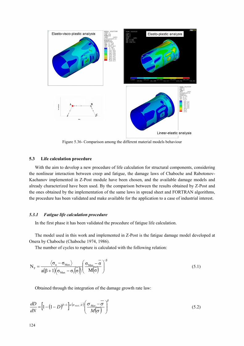
124

Figure 5.36- Comparison among the different material models behaviour

5.3 Life calculation procedure

With the aim to develop a new procedure of life calculation for structural components, considering

the nonlinear interaction between creep and fatigue, the damage laws of Chaboche and Rabotonov-

Kachanov implemented in Z-Post module have been chosen, and the available damage models and

already characterized have been used. By the comparison between the results obtained by Z-Post and

the ones obtained by the implementation of the same laws in spread sheet and FORTRAN algorithms,

the procedure has been validated and make available for the application to a case of industrial interest.

5.3.1 Fatigue life calculation procedure

In the first phase it has been validated the procedure of fatigue life calculation.

The model used in this work and implemented in Z-Post is the fatigue damage model developed at

Onera by Chaboche (Chaboche 1974, 1986).

The number of cycles to rupture is calculated with the following relation:

β

Max

lMax

MaxuF

σM

σσ

σσσ1βa

σσN

(5.1)

Obtained through the integration of the damage growth rate law:

MD

dN

dD MaxMAX ,111 (5.2)

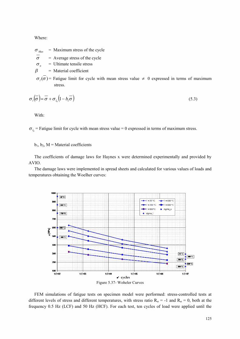
125

Where:

Max = Maximum stress of the cycle

= Average stress of the cycle

u = Ultimate tensile stress

= Material coefficient

)( l = Fatigue limit for cycle with mean stress value 0 expressed in terms of maximum

stress.

110

bll (5.3)

With:

0l = Fatigue limit for cycle with mean stress value = 0 expressed in terms of maximum stress.

b1, b2, M = Material coefficients

The coefficients of damage laws for Haynes x were determined experimentally and provided by

AVIO.

The damage laws were implemented in spread sheets and calculated for various values of loads and

temperatures obtaining the Woelher curves:

Figure 5.37- Woheler Curves

FEM simulations of fatigue tests on specimen model were performed: stress-controlled tests at

different levels of stress and different temperatures, with stress ratio R = -1 and R = 0, both at the

frequency 0.5 Hz (LCF) and 50 Hz (HCF). For each test, ten cycles of load were applied until the

126

material stabilization. The stress analysis results of the last cycle (the stabilized one) were post-

processed through Z-Post, applying the Chaboche fatigue model for determining fatigue life of the

component, using average and minimum material properties.

Following, the results of the simulation of the HCF test performed at R = -1, T=20°C, frequency

50 Hz and = 460 MPa. In Figure 5.38, it is shown the stress time history calculated in a node of

utilizable length and in Figure 5.39 the stress contour plot in correspondence of the time step of

maximum load.

Figure 5.38- Stress [MPa] time [s] history in a node of utilizable lenght

Figure 5.39- Stress contour plot in time step corresponding to the application of maximum tensile load and closeup of utilizable lenght

Following the post-processing of the stress analysis results and fatigue life calculation:

127

Figure 5.40- Life contour plot in logaritmic scale on the left and on the right, minimum life value (number ofcycles to rupture) determined in a node of utilizable lenght

Where LNF_S is the number of cycles to failure in logarithmic scale and NF_S is the number of

cycles to failure in linear scale, obtained in a node of utilizable length.

The results obtained by FEM calculations of life have been arranged in Woelher curves.

In Figure 5.41, at different temperatures and in logarithmic scale, it is shown the points in which,

the FEM calculated life has been obtained.

Figure 5.41- Comparisons between the life calculated through spread sheets and through FEM

By the comparisons shown in Figure 5.41, life calculated by the damage law implemented in

spread sheets and the one obtained through FEM simulations of fatigue tests, it has been possible to

validate the procedure of fatigue life calculation.

5.3.2 Creep life calculation procedure

In this phase, it has been validated the procedure of creep life calculation.

The model used in this work and implemented in Z-Post is the Rabotnov-Kachanov creep model

(Kachanov 1958, Rabotonov 1963, Vozza 2002).

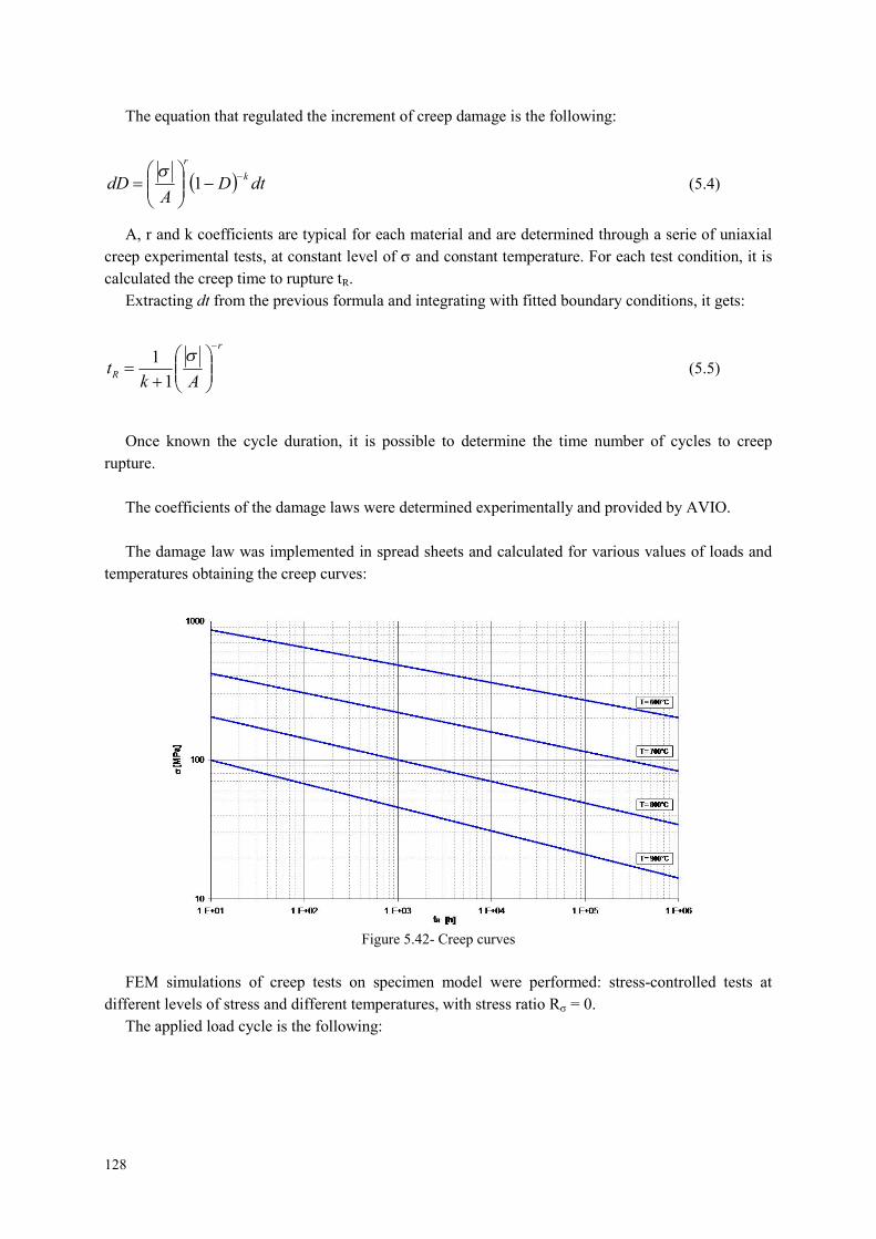
128

The equation that regulated the increment of creep damage is the following:

dtDA

dDk

r

1

(5.4)

A, r and k coefficients are typical for each material and are determined through a serie of uniaxial

creep experimental tests, at constant level of and constant temperature. For each test condition, it is

calculated the creep time to rupture tR.

Extracting dt from the previous formula and integrating with fitted boundary conditions, it gets:

r

RAk

t

1

1(5.5)

Once known the cycle duration, it is possible to determine the time number of cycles to creep

rupture.

The coefficients of the damage laws were determined experimentally and provided by AVIO.

The damage law was implemented in spread sheets and calculated for various values of loads and

temperatures obtaining the creep curves:

Figure 5.42- Creep curves

FEM simulations of creep tests on specimen model were performed: stress-controlled tests at

different levels of stress and different temperatures, with stress ratio R = 0.

The applied load cycle is the following:

129

Figure 5.43- Creep test load cycle

In which: load time t1 = 10s, unload time t3 = 10s, hold time t2 = 3600s

The stress analysis results were post-processed through Z-Post, applying the Rabotonov-Kachanov

creep model for determining creep life of the component, using average and minimum material

properties.

Following, the results of the simulation of the creep test performed at R = 0, T=600°C and = 450

MPa. In Figure 5.44, the stress contour plot in correspondence of the time step t = 10s at the end of

loading phase and corresponding to the application of maximum tensile load. In the same figure, on

the right, the close up of utilizable lenght.

Figure 5.44- Stress contour plot in time step t=10s and close up of utilizable lenght

Following the post-processing of the stress analysis results and creep life calculation:

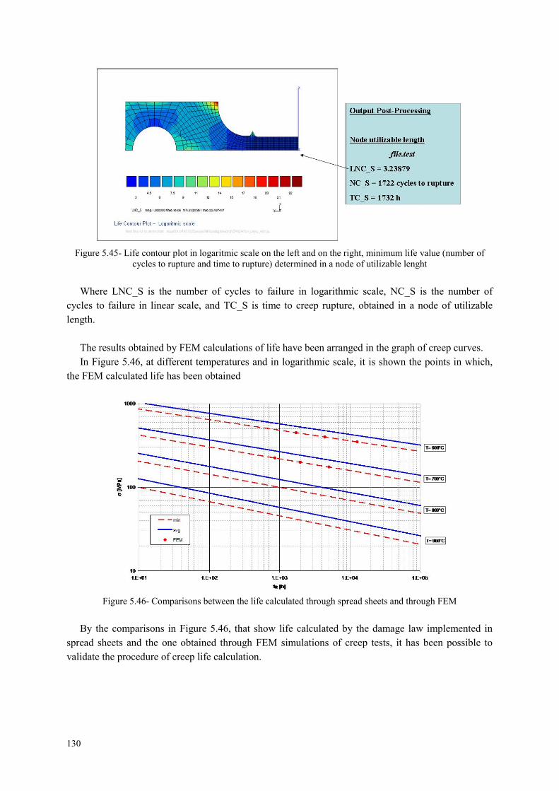
130

Figure 5.45- Life contour plot in logaritmic scale on the left and on the right, minimum life value (number ofcycles to rupture and time to rupture) determined in a node of utilizable lenght

Where LNC_S is the number of cycles to failure in logarithmic scale, NC_S is the number of

cycles to failure in linear scale, and TC_S is time to creep rupture, obtained in a node of utilizable

length.

The results obtained by FEM calculations of life have been arranged in the graph of creep curves.

In Figure 5.46, at different temperatures and in logarithmic scale, it is shown the points in which,

the FEM calculated life has been obtained

Figure 5.46- Comparisons between the life calculated through spread sheets and through FEM

By the comparisons in Figure 5.46, that show life calculated by the damage law implemented in

spread sheets and the one obtained through FEM simulations of creep tests, it has been possible to

validate the procedure of creep life calculation.

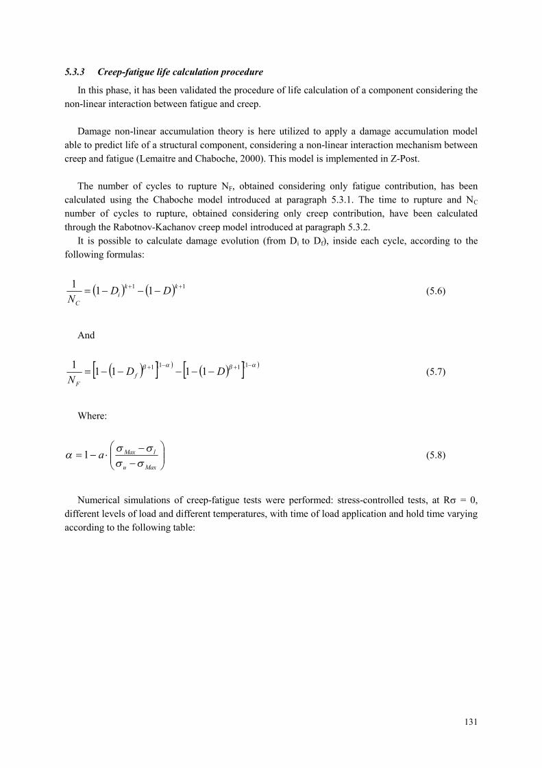
131

5.3.3 Creep-fatigue life calculation procedure

In this phase, it has been validated the procedure of life calculation of a component considering the

non-linear interaction between fatigue and creep.

Damage non-linear accumulation theory is here utilized to apply a damage accumulation model

able to predict life of a structural component, considering a non-linear interaction mechanism between

creep and fatigue (Lemaitre and Chaboche, 2000). This model is implemented in Z-Post.

The number of cycles to rupture NF, obtained considering only fatigue contribution, has been

calculated using the Chaboche model introduced at paragraph 5.3.1. The time to rupture and NC

number of cycles to rupture, obtained considering only creep contribution, have been calculated

through the Rabotnov-Kachanov creep model introduced at paragraph 5.3.2.

It is possible to calculate damage evolution (from Di to Df), inside each cycle, according to the

following formulas:

1111

1

kk

i

C

DDN

(5.6)

And

11111111

1DD

Nf

F

(5.7)

Where:

Maxu

lMaxa

1 (5.8)

Numerical simulations of creep-fatigue tests were performed: stress-controlled tests, at R = 0,

different levels of load and different temperatures, with time of load application and hold time varying

according to the following table:

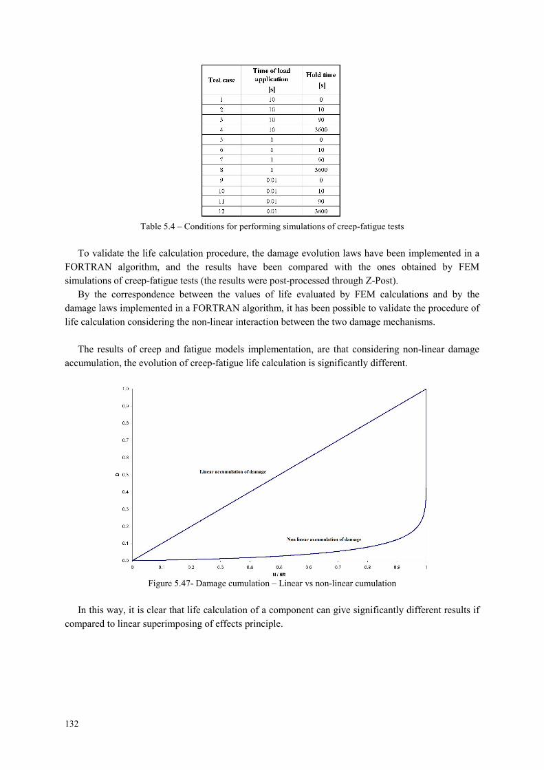
132

Table 5.4 – Conditions for performing simulations of creep-fatigue tests

To validate the life calculation procedure, the damage evolution laws have been implemented in a

FORTRAN algorithm, and the results have been compared with the ones obtained by FEM

simulations of creep-fatigue tests (the results were post-processed through Z-Post).

By the correspondence between the values of life evaluated by FEM calculations and by the

damage laws implemented in a FORTRAN algorithm, it has been possible to validate the procedure of

life calculation considering the non-linear interaction between the two damage mechanisms.

The results of creep and fatigue models implementation, are that considering non-linear damage

accumulation, the evolution of creep-fatigue life calculation is significantly different.

Figure 5.47- Damage cumulation – Linear vs non-linear cumulation

In this way, it is clear that life calculation of a component can give significantly different results if

compared to linear superimposing of effects principle.

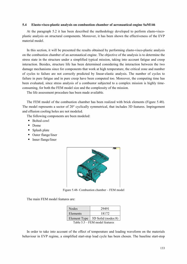
133

5.4 Elasto-visco-plastic analysis on combustion chamber of aeronautical engine SaM146

At the paragraph 5.2 it has been described the methodology developed to perform elasto-visco-

plastic analysis on structural components. Moreover, it has been shown the effectiveness of the EVP

material model.

In this section, it will be presented the results obtained by performing elasto-visco-plastic analysis

on the combustion chamber of an aeronautical engine. The objective of the analysis is to determine the

stress state in the structure under a simplified typical mission, taking into account fatigue and creep

interaction. Besides, structure life has been determined considering the interaction between the two

damage mechanisms since for components that work at high temperature, the critical zone and number

of cycles to failure are not correctly predicted by linear-elastic analysis. The number of cycles to

failure in pure fatigue and in pure creep have been computed too. Moreover, the computing time has

been evaluated, since stress analysis of a combustor subjected to a complex mission is highly time-

consuming, for both the FEM model size and the complessity of the mission.

The life assessment procedure has been made available.

The FEM model of the combustion chamber has been realized with brick elements (Figure 5.48).

The model represents a sector of 20° cyclically symmetrical, that includes 3D features. Impingement

and effusion cooling holes are not modeled.

The following components are been modeled:

Bolted cowl

Dome

Splash plate

Outer flange/liner

Inner flange/liner

Figure 5.48- Combustion chamber – FEM model

The main FEM model features are:

Nodes 29491

Elements 18172

Element Type 3D Solid (nodes:8)Table 5.5 – FEM model features

In order to take into account of the effect of temperature and loading waveform on the materials

behaviour in EVP regime, a simplified start-stop load cycle has been chosen. The baseline start-stop

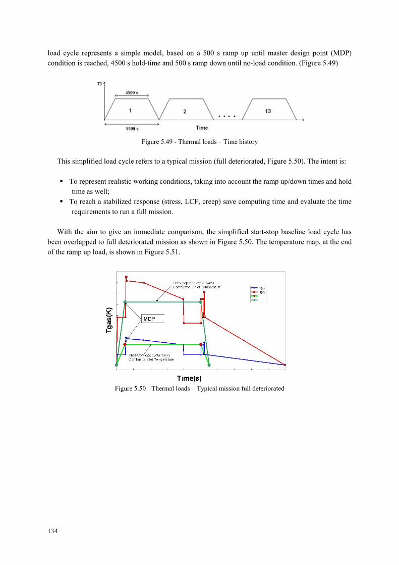
134

load cycle represents a simple model, based on a 500 s ramp up until master design point (MDP)

condition is reached, 4500 s hold-time and 500 s ramp down until no-load condition. (Figure 5.49)

Figure 5.49 - Thermal loads – Time history

This simplified load cycle refers to a typical mission (full deteriorated, Figure 5.50). The intent is:

To represent realistic working conditions, taking into account the ramp up/down times and hold

time as well;

To reach a stabilized response (stress, LCF, creep) save computing time and evaluate the time

requirements to run a full mission.

With the aim to give an immediate comparison, the simplified start-stop baseline load cycle has

been overlapped to full deteriorated mission as shown in Figure 5.50. The temperature map, at the end

of the ramp up load, is shown in Figure 5.51.

Figure 5.50 - Thermal loads – Typical mission full deteriorated

135

Figure 5.51 - Thermal loads – Maximum values [°C]

Following, it is shown the FEM model boundary conditions.

Cyclic symmetry constraints have been applied on the cut sections of the symmetric base sector

(Figure 5.52).

Figure 5.52 – FEM model boundary condition - Cyclic symmetry constraints

On the bolted head flanges area, the average displacements in the tangential direction have been

imposed equal to zero. On the flanges outer edges, axial constraints have been imposed (Figure 5.53).

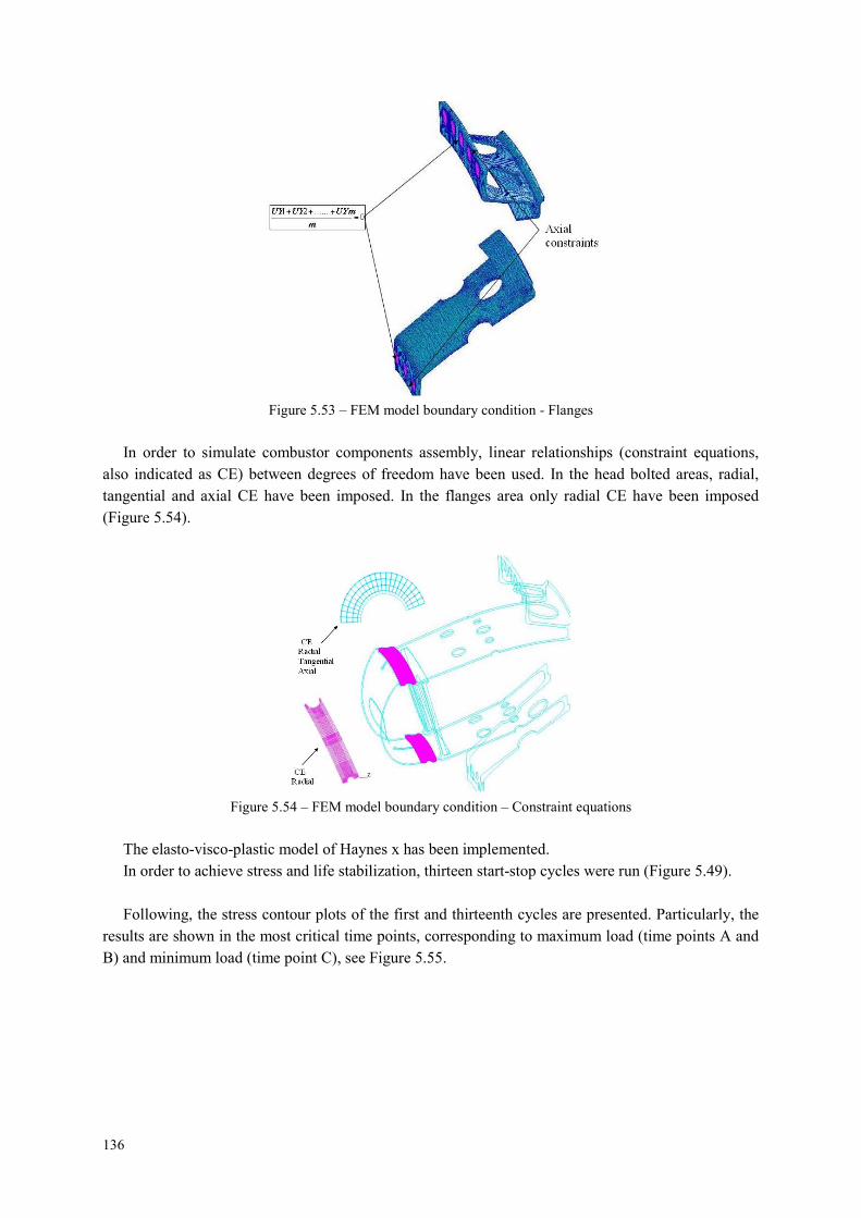
136

Figure 5.53 – FEM model boundary condition - Flanges

In order to simulate combustor components assembly, linear relationships (constraint equations,

also indicated as CE) between degrees of freedom have been used. In the head bolted areas, radial,

tangential and axial CE have been imposed. In the flanges area only radial CE have been imposed

(Figure 5.54).

Figure 5.54 – FEM model boundary condition – Constraint equations

The elasto-visco-plastic model of Haynes x has been implemented.

In order to achieve stress and life stabilization, thirteen start-stop cycles were run (Figure 5.49).

Following, the stress contour plots of the first and thirteenth cycles are presented. Particularly, the

results are shown in the most critical time points, corresponding to maximum load (time points A and

B) and minimum load (time point C), see Figure 5.55.

137

Figure 5.55 – Critical time points

The Figure 5.57 shows Von Mises stress calculated in time point A of the first load cycle (Figure

5.56). Moreover, in the same figure, the node 20107 is the node characterized by the minimum life, as

it will be shown later.

Figure 5.56 – Critical time point A – Cycle 1

Figure 5.57 – Von Mises stress contour plot in time point A of the first cycle

In Figure 5.58, it is shown Von Mises stress calculated in point B of the first cycle, and it is

possible to observe the stress relaxation in comparison with the Von Mises stress calculated in point

A.

138

Figure 5.58 – Von Mises contour plot in time point B of the first cycle

In Figure 5.59 it is shown the results obtained in the last critical time point, C, of the first cycle.

Figure 5.59 – Von Mises contour plot in time point C of the first cycle

Following, from the Figure 5.60 to Figure 5.62, the Von Mises stress calculated in the same critical

time points (A,B,C) but in the last load cycle, are now presented.

139

Figure 5.60 – Von Mises contour plot in time point A of the thirteen cycle

Figure 5.61 – Von Mises contour plot in time point B of the thirteen cycle

Figure 5.62 – Von Mises contour plot in time point C of the thirteen cycle

Following, the most significant analysis results.

140

In Figure 5.63, it is shown the stress time history of the first cycle calculated in the critical node

20107 (minimum life), in which it is possible to observe the material stress relaxation from time point

A to time point B in correspondence of the same maximum load.

Figure 5.63 – Von Mises stress time history of node 20107 – cycle 1

In Figure 5.64 it is shown the stress time history of the thirteen cycle calculated in the same node.

By observing the stress values between the time points A and B, it is possible to consider the

behaviour material stabilized.

The cyclic stress stabilization is more evident in Figure 5.65, where the stress time history of all

cycles, calculated in node 20107, are shown and it is possible to observe also the envelopes of

maximum and minimum stress.

Figure 5.64 – Von Mises stress time history in node 20107 – cycle 13

141

Figure 5.65 – Von Mises stress time history in node 20107 – all cycles

In order to verify the material stabilization, the envelopes of maximum and minimum stress are

also presented in the Table 5.6 and Table 5.7. By the values reported in the tables, it is possible to

observe that the stress variation between the two final instants is less than 1.5%. This lets us to

consider the material behaviour stabilized.

Table 5.6 – Maximum stress envelope

Table 5.7 Minimum stress envelope

142

It is possible to conclude that the results obtained by elasto-visco-plastic analysis on a real

component are in agreement with expected results, in fact the implementation in FEM codes of

complex material models, allows to simulate the real material behaviour and to take into account the

non-linear interaction between creep and fatigue for structural analysis.

Moreover, one of the objectives of the analysis has been also to evaluate the computing CPU time,

in order to evaluate the time requirements to run a full mission, in a next phase of the activity. In

particular, the total CPU time at the end of the first start-stop load cycle has been 35078 seconds (9.74

hours).

5.5 Evaluation of creep and fatigue life

The methodology of life calculation, previously applied and validated on specimens used for

fatigue-creep tests, has been here applied to a real component.

In fact, a further objective of the analysis performed on the combustion chamber was to make

available the life evaluation procedure, by starting from the implementation of an elasto-visco-plastic

material model able to take into account the nonlinear interaction between creep and fatigue.

The life of the structure has been calculated through the module Z-Post of Z-Mat, which allows to

post-processing the results obtained by the elasto-visco-plastic analysis. In particular, the local post-

processing allows studying the variables evolution in the time, once fixed a part of the structure. The

calculation is made in nodes, starting from the data saved in a file given in input to Z-Post, together

with the stress analysis results file and the Z-Mat file containing the values of coefficients material

model. Z-Post module implements various damage models and allows calculating component life

under complex cyclic loads.

The damage non-linear accumulation theory has been utilized to apply a damage accumulation

model able to predict life of the structural component considering a non-linear interaction mechanism

between creep and fatigue. The number of cycle to failure, NF, obtained by considering pure fatigue

and the number of cycle to failure, NC, obtained by pure creep, have been calculated respectively by

Chaboche and Rabotnov-Kachanov theories introduced at paragraphs 5.3.1 and 5.3.2.

In according with these laws, the evolution of the damage (from Di to Df) inside each cycle has

been calculated by the equations introduced at paragraph 5.3.3.

Following, the life calculation results are presented. In particular, it is shown the hysteresis cycles

obtained by stress analysis and calculated in the critical nodes and and the life versus cycles plots

calculated in the same nodes:

In node 20107 (located in outer liner) minimum creep life has been verified.

In node 20194 (located in outer liner) minimum fatigue life has been verified.

The Figure 5.66 shows the hysteresis cycles calculated in node 20107 and the Figure 5.67 shows

the values of creep life versus cycles.

143

Figure 5.66 – Hysteresis cycle in node 20107

Figure 5.67 – Creep life in node 20107

In Figure 5.68 it is shown the creep life contour plot in logarithmic scale on the structure. It is

highlighted the critical area, where it is located the node in which minimum creep life has been

determined.

Figure 5.68 – Creep life contour plot

In Figure 5.69, it is shown the position of the node 20194 in FEM model. This is the node where

minimum fatigue life has been verified.

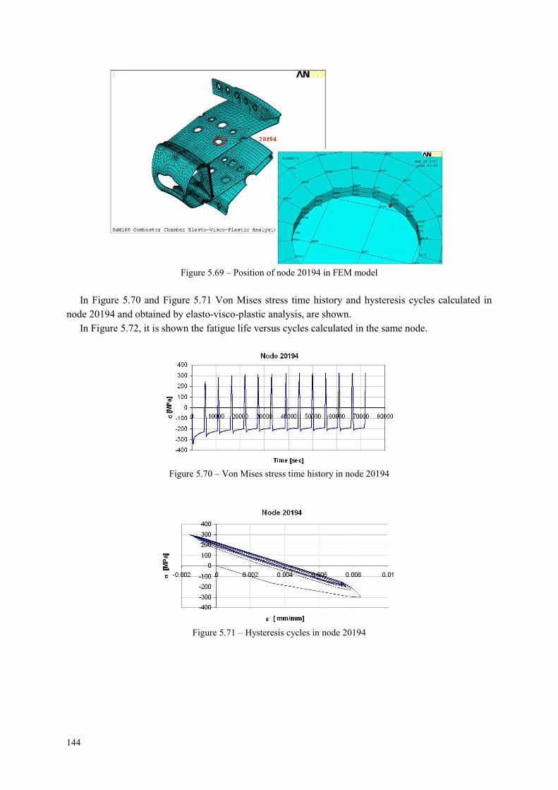
144

Figure 5.69 – Position of node 20194 in FEM model

In Figure 5.70 and Figure 5.71 Von Mises stress time history and hysteresis cycles calculated in

node 20194 and obtained by elasto-visco-plastic analysis, are shown.

In Figure 5.72, it is shown the fatigue life versus cycles calculated in the same node.

Figure 5.70 – Von Mises stress time history in node 20194

Figure 5.71 – Hysteresis cycles in node 20194

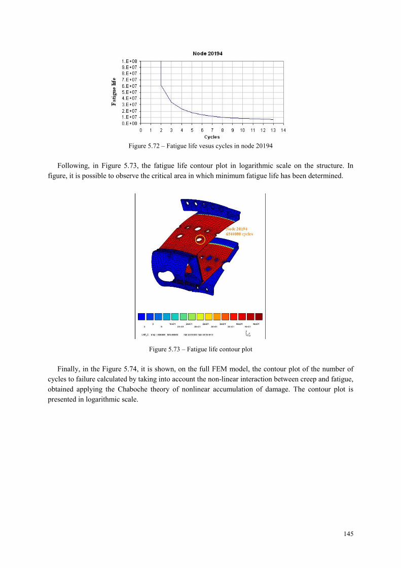
145

Figure 5.72 – Fatigue life vesus cycles in node 20194

Following, in Figure 5.73, the fatigue life contour plot in logarithmic scale on the structure. In

figure, it is possible to observe the critical area in which minimum fatigue life has been determined.

Figure 5.73 – Fatigue life contour plot

Finally, in the Figure 5.74, it is shown, on the full FEM model, the contour plot of the number of

cycles to failure calculated by taking into account the non-linear interaction between creep and fatigue,

obtained applying the Chaboche theory of nonlinear accumulation of damage. The contour plot is

presented in logarithmic scale.

146

Figure 5.74 – Life contour plot

In the table, it is presented a summary of the results obtained:

Table 5.8 – A summary of results

In particular in the Table 5.8, it is shown the maximum and minimum stress calculated in the two

critical nodes, in the thirteen cycle, and the values of medium and alternate stress. Moreover, it is

possible to observe the values of minimum number of cycle to failure (NR), and the number of cycle

to failure calculated in pure fatigue (NF) and pure creep (NC). The results show that the critical area is

located at node 20107.

In this way, a new procedure of life calculation has been developed and make available in order to

take into account the interaction between the two damage mechanisms for evaluating in a more careful

way the operative life of structures.

The developed procedure for implementing in FEM codes complex material models, able to

simulate the real behaviour of materials and to take into account the non-linear interaction between

creep and fatigue for structural analysis and life prediction, allows improving significantly the

designing of structural components. In fact, the capability of reproducing the real material behaviour

and predicting the component life in a more dependable way, allow reducing the traditional factors of

safety that are overly conservative and preventing from achieving the optimal efficiency in structural

designing process.

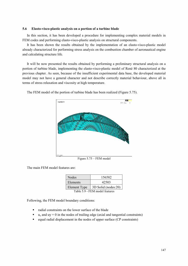
147

5.6 Elasto-visco-plastic analysis on a portion of a turbine blade

In this section, it has been developed a procedure for implementing complex material models in

FEM codes and performing elasto-visco-plastic analysis on structural components.

It has been shown the results obtained by the implementation of an elasto-visco-plastic model

already characterized for performing stress analysis on the combustion chamber of aeronautical engine

and calculating structure life.

It will be now presented the results obtained by performing a preliminary structural analysis on a

portion of turbine blade, implementing the elasto-visco-plastic model of Renè 80 characterized at the

previous chapter. As seen, because of the insufficient experimental data base, the developed material

model may not have a general character and not describe correctly material behaviour, above all in

terms of stress relaxation and viscosity at high temperature.

The FEM model of the portion of turbine blade has been realized (Figure 5.75).

Figure 5.75 – FEM model

The main FEM model features are:

Nodes 156582

Elements 42503

Element Type 3D Solid (nodes:20)Table 5.9 - FEM model features

Following, the FEM model boundary conditions:

radial constraints on the lower surface of the blade

ux and uy = 0 in the nodes of trailing edge (axial and tangential constraints)

equal radial displacement in the nodes of upper surface (CP constraints)

148

Figure 5.76 – FEM model constraints

Figure 5.77 – FEM model – CP constraints

The blade is lapped on the airfoil by hot gas in expansion (T > 800°C in base-load) and on the

internal channels by the air spilled by compressor (T > 300°C in base-load). By convection, hot gases

give up heat to the blade through airfoil surface; while the air that laps the surface of internal channels

takes away heat (see Figure 5.78).

Figure 5.78 – Conditions of thermal exchange

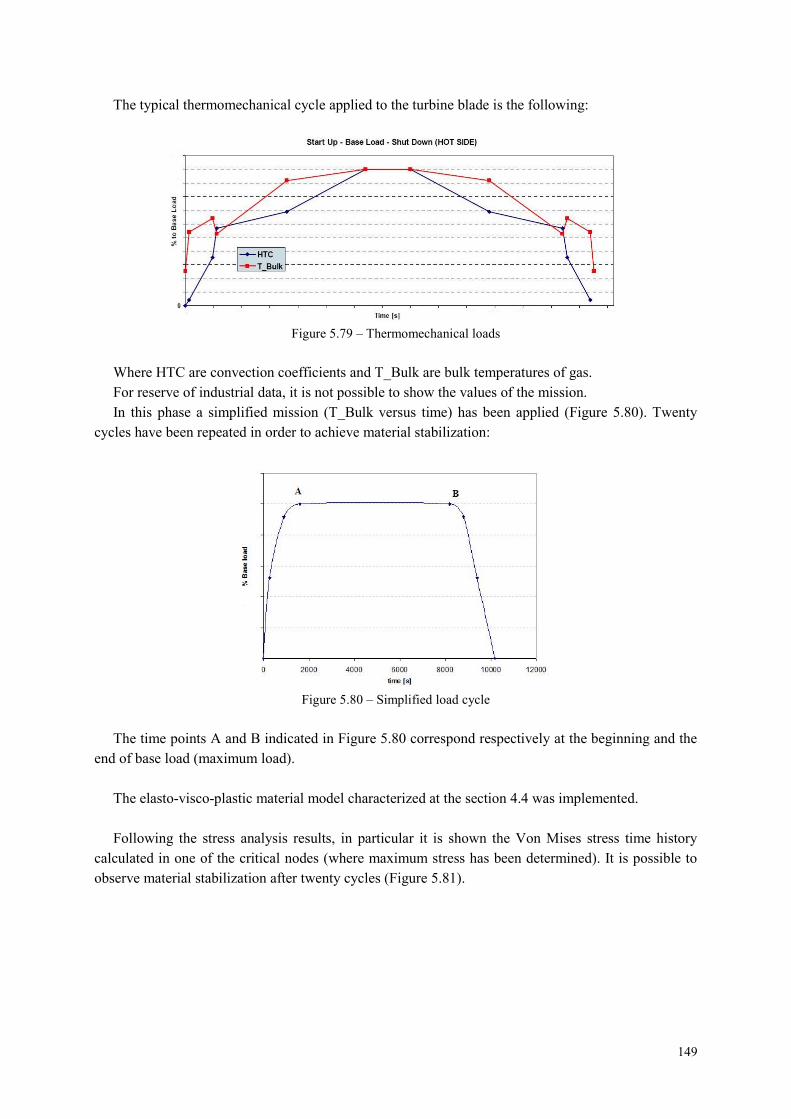
149

The typical thermomechanical cycle applied to the turbine blade is the following:

Figure 5.79 – Thermomechanical loads

Where HTC are convection coefficients and T_Bulk are bulk temperatures of gas.

For reserve of industrial data, it is not possible to show the values of the mission.

In this phase a simplified mission (T_Bulk versus time) has been applied (Figure 5.80). Twenty

cycles have been repeated in order to achieve material stabilization:

Figure 5.80 – Simplified load cycle

The time points A and B indicated in Figure 5.80 correspond respectively at the beginning and the

end of base load (maximum load).

The elasto-visco-plastic material model characterized at the section 4.4 was implemented.

Following the stress analysis results, in particular it is shown the Von Mises stress time history

calculated in one of the critical nodes (where maximum stress has been determined). It is possible to

observe material stabilization after twenty cycles (Figure 5.81).

150

Figure 5.81 – Von Mises stress time history calculated in a critical node – all cycles

Following, the Von Mises stress contour plot calculated in the first cycle at the beginning of the

base-load (maximum load): time point t = 1600s (Figure 5.82).

Figure 5.82 – Von Mises stress contour plot calculated in the first cycle at t = 1600s

Following, the Von Mises stress contour plot calculated in the first cycle at the end of the base-load

(maximum load): time point t = 8200s (Figure 5.83).

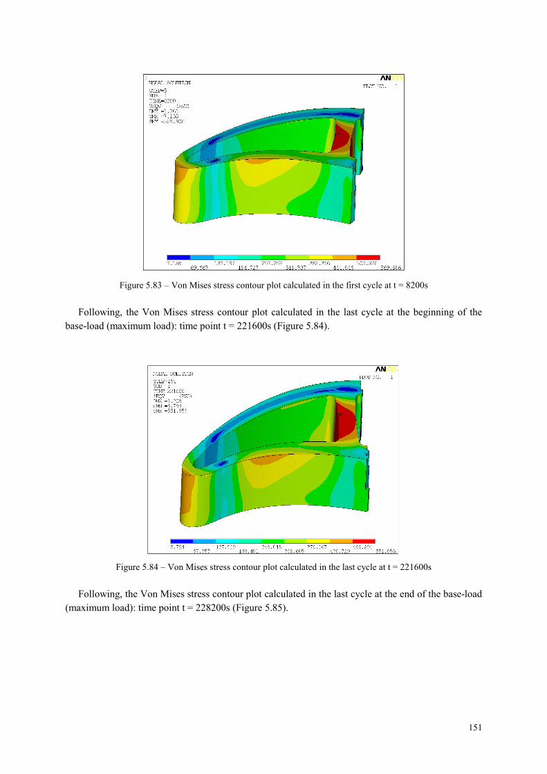
151

Figure 5.83 – Von Mises stress contour plot calculated in the first cycle at t = 8200s

Following, the Von Mises stress contour plot calculated in the last cycle at the beginning of the

base-load (maximum load): time point t = 221600s (Figure 5.84).

Figure 5.84 – Von Mises stress contour plot calculated in the last cycle at t = 221600s

Following, the Von Mises stress contour plot calculated in the last cycle at the end of the base-load

(maximum load): time point t = 228200s (Figure 5.85).

152

Figure 5.85 – Von Mises stress contour plot calculated in the last cycle at t = 228200s

From the Figure 5.82 and Figure 5.83 it is possible to observe the time-dependent material model

behaviour: the results show, in fact, the stress relaxation that the component has during its steady state

condition.

The two stress contour plots show the same structure, in the same cycle at the end of the start up

sequence and before the shut down procedure. In this specific case 6600s have been considered.

From the Figure 5.84 and Figure 5.85 it is possible to observe the stabilization of material: in the

last cycle, in fact, the stress remain constant from the time point A to B (from the beginning to the end

of base load).

It is necessary to point out that the highlighted stress relaxation (Figure 5.82 and Figure 5.83) is

low, since the material model is not still optimized.

As seen, during the process of material characterization it was not possible to optimize the viscous

parameters of the model because of dependable experimental data (tensile tests at different strain rate,

relaxation tests) were lacking. For this reason, as expected, the stress analysis results have shown a

predictive capability of the model not still sufficient. However, the presently obtained numerical

results may be considered to be reasonable, if the scarcity of available experimental data is kept in

mind.

Better results may be obtained integrating the experimental data base with new tests opportunely

designed for the characterization process and determining the optimized set of model coefficients.

153

6 Concluding Remarks

To introduce innovation in high temperature components design, it is essential to accurately assess

structural integrity of the components for long-term elevated temperature service and thereby to

reduce the unduly overconservatism in the design. In order to evaluate creep-fatigue damage and

cumulative inelastic strains, it is required to perform detailed inelastic analysis for predicting

accurately the stress/strain history taking into account both time independent and time dependent

material deformation behaviour. Since the stress/strain response of the components is closely related to

life prediction, the reliability of life prediction depends strongly on the adequacy of the constitutive

models employed in the analysis.

Among various viscoplastic models available in literature, the Chaboche viscoplastic model is

found to be superior for high temperature components applications (as gas turbine blades and

combustion camber of jet engines) because of its ability to simulate, with reasonable accuracy, all the

essential mechanical behaviour of Ni-base superalloys in the temperature range of 400-1000°C under

monotonic and cyclic loading conditions.

The strength of this model is in the possibility to use multi-potential mechanisms for cases of time

independent plasticity in combination with viscoplastic deformation. Potentials represent inelastic

dissipations which describe the evolution of independent inelastic deformation mechanisms. In this

way, total strain may be partitioned into the reversible or elastic strain and the irreversible or inelastic

strain. The latter can be further separated into plastic and viscoplastic strain. The result is refined

modelling of a wide range of strain rates associated with different deformation mechanisms, in this

way each potential can have its own flow law and hardening mechanism independently from the other

ones. Besides, Chaboche model allows the superimposition of isotropic hardening on nonlinear

kinematic hardening resulting in a modification of the elastic domain by translation and uniform

expansion. This allows describing the progression of hardening for materials subjected to cyclic loads.

Besides, differently from others kinematic hardening models analysed in literature (for example Prager

model), the evolution of the kinematic variable in the time is defined in way to take into account the

effects due to the deformation history. This model allows considering a hardening which changes with

continuity, with the advantage to describe the nonlinearity of cyclic plastic deformation process.

However, it has been shown that one major limitation of Chaboche model is in its high number of

parameters and accordingly in a lot of material data required to identify them.

The developed work has allowed a detailed analysis of material characterization process and has

led to the application of the Chaboche elasto-visco-plastic model to a Nickel base superalloy used in

high temperature components of gas turbines and jet engines. The constitutive equations were defined

in way to be able to predict material behaviour under repeated cyclic loads and high temperatures. In

particular, two dissipation potentials have been utilized to accurately capture the material loading-rate

sensitivity, since each of them describe the evolution mechanisms of inelastic deformations associated

respectively to slow and high strain rates. Moreover, it has been show how the superposition of two

kinematic hardening models provide a significantly better response in representing the real material

behaviour over the entire strain range, compared to a single kinematic hardening model. This choice

allowed smoothing out the transition from linear to nonlinear behaviour and modelling short and long-

range hardening mechanisms.

154

The developed elasto-visco-plastic model with isotropic and kinematic hardening combines

plasticity and creep and allow taking into account of material behaviour rate dependence.

Material characterization process has been developed through the following phases:

Choice of the characteristic tests and interpretation of the mechanical quantities (t); p(t).

This choice depends on the envisaged field of application:

initial loading

stabilized cycle

transient cyclic effects.

Identification of model coefficients: this has been the most difficult step (high number of

involved parameters).

Identification can be defined as the work consisting in specifying the functions which appear in the

model and in finding the numerical values of the coefficients which define the functions for each

material. It has been shown how this represents a very difficult task since it does not follow any

rigorous rule and in which experience and “art of building a model” play a major role in steering

between theory and experiment. This involves a procedure of parameters identification that is still too

artful and far to be standardized.

The initial parameters, given by tentative, have been fitted to the real curves through an iterative

process of optimization based on mean square values technique. It has been necessary to turn out to a

step-by-step procedure of characterization, adding tests and the corresponding sensitive parameters

progressively into the optimization loop. In a such procedure, the previously calibrated coefficients

provide good starting points for the next step, thus allowing the algorithm to escape from local

minima. At the end, all tests have to be added and all coefficients identified at the same time, for

obtaining a good set of coefficients.

However, in spite of a step by step procedure was applied, many problems of convergence of the

optimization tool were verified. In fact, many coefficients are strongly depending one each other;

further in absence of a good experimental data base, a non correct identification of one of these

parameters, implies the not convergence of the solution during the optimization process.

As it was introduced at the beginning of the work and subsequently examined, the most important

and often times most difficult, aspect of modeling material behaviour at elevated temperature is

obtaining the required material functions for viscoplaticity and associated material parameters. The

difficulty associated with this process stems from not only the variety in mathematical forms for the

material functions, but also the fact that given the material functions there is no unique set of material

parameters for any given load path. Therefore, numerous iterations and difficult compromises are

required before a final set of material parameters (for the assumed material functions) can be obtained.

The developed work has highlighted how these aspects are particularly true when dealing with models

that possess a very large number of material constants that:

are often lacking in their direct physical interpretation

may have vastly different magnitudes

are highly interactive one each other.

On the other hand, the number of coefficients represents the price to pay for obtaining a model which

has the ambition of becoming a law. In fact, the result of material characterization process has to be a

model with a general character, so that while identified only by a restricted number of experiments, it

is representative of other types of experiments with a predictive capability. The totality of the

situations verified by a model is its field of validity. This characterizes the goodness of the model and

155

is expressed qualitatively by the set of all possible variation histories of the variables and

quantitatively by the range of the variations within which the model agrees with the physics.

In Chapter 4, it has been widely shown that a model cannot be identified correctly unless a sufficient

number of test results are available, which embrace a significant range of variation of each parameter.

Otherwise, we run the risk of not determining one or more coefficients well enough. Moreover, it has

been verified how quality of performed experiments has affected the characterization process leading

to a significant reduction of utilizable experimental tests because of too scattered data and numerous

uncertainties, losing in material model generality.

As shown and already dealt with detail at the section on the design of experiments, some guidelines

have been provided in order to perform a complete process of material characterization and to

determine a set of optimized parameters for Chaboche elasto-visco-plastic model. First of all, two

different groups of tests have to be designed: for characterization and validation processes

respectively. In particular, tests within the reversible domain (i.e., creep with recovery upon complete

unloading, and relaxation) and experiments conducted within the irreversible domain (i.e., relaxation,

conventional creep, multi-step creep, tensile curves at different total strain rates) have to be used for

characterization; while multiple-step relaxation, cyclic and plasticity/creep interaction tests have to be

reserved for validating the predictive behaviour of the model.

It was then shown the necessity to separate the characterization process in more stages in order to

reduce the convergence problems of solution:

1. Determining viscous flow and initial yield stress using tensile curves at different total strain

rates. This kind of tests allows calibrating the viscous effects and the dependence of material

behaviour by loading-rate.

2. Determining hardening parameters by LCF tests and LCF-step tests, in particular by cyclic

curve and stabilized loops.

3. Determining thermal recovery parameters by providing relaxation, conventional creep and

multi-step creep tests while keeping the flow and hardening parameters estimates from step 1

and 2 fixed. These kinds of tests allow describing the time-dependent (short-term and long-

term) material behaviour.

4. Fit all tests at one time to obtain final parameter estimates, this is accomplished by allowing

all visco-plastic parameters to be active (using the material parameters found in steps 1, 2 and

3 as initial starting values) but with tight upper and lower bounds around each parameter.

In the designing of experimental tests, it is important to consider that if one went to focus on only

one type of loading condition, superior correlations could of course be achieved for that class of

loading. However, predictions of other classes of loading may severely suffer. For example, during a

separate characterization process involving only tensile tests, excellent correlation was obtained, but at

the expense of poor creep and relaxation behaviour for a given set of material parameters. Conversely,

when the model was calibrated for creep responses, poorer tensile and relaxation behaviours were

similarly predicted. Thus when judging the “goodness” of a given model, it must keep in mind the

appropriate required “data content” for accurately capturing the full range of material behaviour of

interest. For an identical material and model, it may be necessary to define several sets of coefficients,

each better suited to a domain of variation or to a load type, for example, rapid transient loads, short-

term loads, long-term loads and stationary loads.

156

The careful analysis of material characterization process has allowed developing a procedure for

implementing in FEM codes complex material models, able to simulate the real material behaviour

and to take into account the non-linear interaction between creep and fatigue for structural analysis

and life prediction. A procedure of structural analysis has been developed through the comparison

with procedures of tested validity, in way to allow a correct and safe implementation of elasto-visco-

plastic material models. In particular, starting from an elasto-visco-plastic material model, already

characterized and validated, it has been possible to test its effectiveness by performing comparison

analysis with known models in linear-elastic and elasto-plastic fields.

As discussed in Capther 5, the procedure has been developed and validated on a test case and then

applied to a combustion camber of aeronautical engine. The obtained results are in agreement with the

expected ones: the implementation of an elasto-visco-plastic model in FEM code has allowed

simulating the physical phenomena, stress relaxation and cycle stabilization, which may be

appreciated only through an analysis performed with a rate dependent material model.

As a matter of fact, the elasto-visco-plastic model doesn’t consider the time variable as a simple

counter, that scans the succession of load configurations, but associates to it the real physical meaning.

In this way both the loads application and material behaviour become rate dependent.

For this reason, the material model is able to simulate at once, fatigue and creep under

thermomechanical loads for long time and the effect of “diffusion” that creep causes.

Besides, structure life has been determined considering the nonlinear interaction between the two

damage mechanisms since for components that work at high temperatures, critical zone and number of

cycles to failure are not correctly predicted by linear elastic analysis and the simple superimposing of

creep and fatigue damage is too conservative for actual industrial needs.

The important contribute that the present work will provide to industrial applications is in the

development of a procedure that improves significantly the design of structural components through

the implementation of elasto-visco-plastic material models. In fact, the capability of simulating the

real material behaviour and predicting the component life in a more dependable way by taking into

account the nonlinear interaction between fatigue and creep, allow reducing the traditional factors of

safety that are overly conservative and preventing from achieving the optimal efficiency in structural

designing procedure.

It has been shown also the response obtained by implementing the material model not completely

characterized in Chapter 4 because of the available experimental data base was not sufficient. The

results of an elasto-visco-plastic analysis performed on a portion of turbine blade have shown that the

developed model is able to capture the rate dependent material behaviour but, as expected, its

predictive capability is not still sufficient.

As widely shown and examined until now, it is important to highlight that material characterization

process and implementation of complex user-defined material models in FEM software are then the

results of procedures still far off to be standardized and above all are affected by the choice which the

analyst do on the base of his experience. Besides, it is a slow and expensive process and doesn’t assure

the result.

However, the required steps have been highlighted in order to get a correct and complete

characterization process.

157

References

1. Abed, F.H. and Voyiadjis, G.Z., 2005. A consistent modified Zerilli-Armstrong flow stress model

for bbc and fcc metals for elevated temperatures. Acta Mechanica 175, 1-18.

2. Anand, L. and Brown, S., 1987.Constitutive Equations for Large Deformations of Metals a t High

Temperatures. In: Chandra, J., and Srivastav, R.P. (eds.) , C onstitutive Models of Deformation,

SIAM, Philadelphia, pp. 1-26.

3. ANSYS Inc., 2000. Guide to ANSYS User Programmable Features, Publ. No. 001263.

4. Armstrong, P.J. and Frederick, C.O., 1966. A Mathematical Representation of the MuhiaxialBauschinger Effect. C.E.G.B. Report RD/B/N 731.

5. Arnold, S.M., Saleeb, A.F. and Wilt, T.E, 1995. A modeling investigation of thermal and straininduced recovery and non linear hardening in potential based viscoplasticity. J. Engng. Mater.Tech. ASME, Vol. 117, pp. 157-167.

6. Arnold, S.M. and Saleeb, A.F., 1994. On the thermodynamic framework of generalized coupledthermoelastic viscoplastic-damage modelling. Int. J. Plasticity, Vol. 10, No 3, pp. 263-278.

7. ASME Boiler and Pressure Vessel Code, 1974. Sec. III, Case interpretations, Code Case N-47-17.

8. ASTM Metals Handbook: Vols-1-12 American society for metals, Philadelphia

9. Azzouz, F., Cailletaud G., Foerch R., Morine G., Quilici S., and Ragot, P., 2002. Identification ofviscoplastic costitutive and creep-fatigue coefficients to use in Abaqus automotive structuralcalculation with Zmat library

10. Bailey, R.W., 1926. Note on the Softening of Strain-Hardened Metals and Its Relation to Creep.

J. Inst. Met., 35, 27.

11. Bathe, K. J., 1996. Finite Element Procedures. Prentice-Hall, Englewood Cliffs.

12. Bazant, Z.P. and Bhat, P.D.; 1976. Endochronic theory of inelasticity and failure of concrete. J.

Engng. Mech. Div., proc. ASCE, 102, EM4, 701.

13. Bazant, Z.P., 1978. Endochronic inelasticity and incremental plasticity. Int. J. Solids Struct., 14,

691.

14. Benallal, A., Le Gallo, P., Marquis, D., 1989. An experimental investigation of cyclic hardeningof 316 stainless steel and of 2024 aluminium alloy under multiaxial loadings. NuclearEngineering and Design 114, 345–353.

15. Bertram, A., 2003. Finite thermoplasticity based on isomorphisms. International Journal ofPlasticity 19, 2027–2050.

16. Besseling, J.F., 1958. Theory of elastic, plastic, and creep deformations of an initially isotropicmaterial showing anisotropic strain-hardening, creep recovery, and secondary creep. J. Appl.Mech., 25, 529.

158

17. Bever, M., Holt, D., Titchener, A., 1973. The Stored Energy of Cold Work. Progress in MaterialsScience, vol. 17. Pergamon, Oxford.

18. Bodner, S.R. and Partom, Y., 1975. Constitutive Equations for Elastic-Viscoplastic Strain-

Hardening Materials. J. Appl. Mech., 42, 385.

19. Bodner, S.R., Lindenfeld, A., 1995. Constitutive modelling of the stored energy of cold workunder cyclic loading. European Journal of Mechanics A – Solids 14, 333–348.

20. Bruhns, O., Lehmann, T., Pape, A., 1992. On the description of transient cyclic hardeningbehaviour of mild steel CK15. International Journal of Plasticity 8, 331–359.

21. Bucher, A., Go¨rke, U.-J., Kreißig, R., 2004. A material model for finite elasto-plasticdeformations considering a substructure. International Journal of Plasticity 20, 619–642.

22. Cernocky, E.P. and Kremple, E., 1979. A nonlinear uniaxial integral constitutive equationincorporating rate effects, creep and relaxation, Int. J. Nonlinear Mech. 14, 183-203

23. Cernocky, E.P. and Kremple, E., 1980. A theory of viscoplasticity based on infinitesimal totalstrain. Acta Mech., 36, 263-289

24. Chaboche, J.L., 1974. Une loi différentielle d’endommagement de fatigue avec cumulation nonlinéaire, Extrait de la Revue Francaise de Métallurgie, No.50-51, pp.71-82.

25. Chaboche, J., 1996. Unified cyclic visco-plastic constitutive equations: development, capabilities,and thermodynamic framework. In: Krausz, A., Krausz, K. (Eds.), Unified Constitutive Laws ofPlastic Deformation. Academic Press, New York, pp. 1–68.

26. Chaboche, J., Lemaitre, J., 1990. Mechanics of Solid Materials. Cambridge Press, Cambridge,New York.

27. Chaboche, J.L., 1977. Visco-plastic constitutive equations for the description of cyclic andanisotropic behaviour of metals. Bulletin de L’Academie Polonaise des Sciences 25, 33–41.

28. Chaboche, J.L., 1983a. Constitutive Equations in Creep-Fracture Damage. EngineeringApproaches to High Temperature Design, WILSHIRE and OWEN (Eds.), Pineridge Press,Swansea.

29. Chaboche, J.L., 1983b. On the Constitutive Equations of Materials under Monotonic or CyclicLoadings. La Rech. Aerosp., 1983-5.

30. Chaboche, J.L., 1986. On the non linear fatigue damage accumulation. International Conferenceon Steel Structures, ONERA TP-121, Budva.

31. Chaboche, J.L., 1986. Time-independent constitutive theories for cyclic plasticity. Int J. Plast., 2,149-188.

32. Chaboche, J.L., 1989a. Constitutive equations for cyclic plasticity and cyclic viscoplasticity. Int.J. Plast., 5, 247-302.

33. Chaboche, J.L. and Nouailhas, D., 1989b. A unified constitutive model for cyclic viscoplasticityand its applications to various stainless steels. ASME J. Engng. Mat. Tech, 111, 424-430.

159

34. Chaboche, J.-L., 1993a. Cyclic visco-plastic constitutive equations, Part I: A thermodynamicallyconsistent formulation. Journal of Applied Mechanics 60, 813–821.

35. Chaboche, J.-L., 1993b. Cyclic visco-plastic constitutive equations, Part I: A thermodynamicallyconsistent formulation, Part II: Stored energy – comparison between models and experiments.Journal of Applied Mechanics 60, 813–828.

36. Chaboche, J.L, and Rousselier, G., 1983. On the plastic and viscoplastic constitutive equations.Journal of Pressure Vessel and Technology 105, 153-164

37. Chan, K.S., Lindholm, U.S., Bodner, S.R., and Walker, K.P., 1984. A Survey of Unified

Constitutive Theories. In: Nonlinear Constitutive Relations for High Temperature Application.

NASA CP-2369, pp. 1-23.

38. Chan, K.S., Bodner, S.R. and Lindholm, U.S., 1988. Phenomenological modeling of hardening

and thermal recovery in metals. ASME J. Eng. Mat. Tech. 110, 1-8.

39. Chan, K.S., Lindholm, U.S., Bodner, S.R., and Walker, K.P., 1989. High temperature inelastic

deformation under uniaxial loading: theory and experiment. ASME J. Eng. Mat. Tech. 111, 345-

353.

40. Chan, K.S. and Lindhoim, U.S., 1990. Inelastic deformation under nonisothermal loading. ASME

J. Eng. Mat. Tech., 112, 15-25.

41. Chrysochoos, A., Maisonneuve, O., Martin, G., Caumon, H., Chezeaux, J., 1989. Plastic anddissipated work and stored energy. Nuclear Engineering and Design 114, 323–333.

42. Coleman, B., Gurtin, M., 1967. Thermodynamics with internal state variables. Journal ofChemical Physics 47, 597–613.

43. Coleman, B., Noll, W., 1963. The thermodynamics of elastic materials with heat conduction andviscosity. Archive for Rational Mechanics and Analysis 13, 167–178.

44. Corum, J.M., Greenstreet, W.L., Liu, K.C., Pugh, C.E. and Swindeman, R.W., 1974. Interimguidelines for detailed inelastic analysis of high temperature reactor system components. ORNL –5014.

45. Costagliola, S., 2008. Creation and validation of a FEM structural calculation procedure for gasturbine design, providing an elasto-visco-plastic material model implementing nonlinearinteraction between fatigue and creep. PhD Thesis. University of Naples, Federico II.

46. Cui, W., 2002. A state-of-the-art review on fatigue life prediction methods for metal structures. J.

Mar. Sci. Techn., 7, pp 43-56.

47. Dafalias, Y.F. and Popov, E.P., 1975. A Model of Nonlinearly Hardening Materials for Complex

Loading. Acta Mech., 21, 173.

48. Dafalias, Y.F. and Popov, E.P., 1976. Plastic internal variables formalism of cyclic plasticity.

ASME J. Appl. Mech. 43, 645-651.

160

49. Delobelle, P. and Lexcellent, C., 1988. Etude experimentale de l’effet de rochet de traction-

torsion d’un acier inoxydable. 17-12 Mo SPH; implications pour la formulation d’un modele

unifie, in Proc of MECAMAT, Int seminar on the inelastic behaviour of solids: models and

utilization, Besancon, France, pp 135-153.

50. Delobelle, P. and Oytana, C., 1984. Experimental study of the flow rules of a 316 stainless steel

at high and low stresses. Nucl. Eng. Des. 83, 333-348.

51. Delobelle, P. and Oytana, C., 1987. Modeling of 316 stainless steel (17.12 SPH mechanical

properties using biaxial experiments, ASME J. Pressure Vessel Tech. 109, 449-459.

52. Delprete, C., Fissore S., Sesana R., and Vercelli A., 2007. Confronto trai modelli costitutivi

plastici per il comportamento ciclico dei materiali. AIAS-XXXVI Convegno Nazionale.

53. Deseri, L., Mares, R., 2000. A class of viscoelastoplastic constitutive models based on themaximum dissipation principle. Mechanics of Materials 32, 389–403.

54. Drucker, D.C., 1991. Constitutive relation for results retrospect and prospect. In Proceedings ofthe 3rd International Conference on Constitutive Laws for Engineering Materials.

55. Estrin, Y. and Mecking, H., 1984. A Unified Phenomenological Description of Work Hardening

and Creep Based on One-Parameter Models. Acta Metall., 32, 57.

56. Fan, J. and Peng, X., 1991. A phisically based constitutive description for nonproportional cyclic

plasticity. Journal of Engineering Materials Technology 113, 254-262.

57. Findley, W.N. and lai, J.S., 1978. Creep and recovery of 2618 Aluminum alloy under combined

stress with a representation by a viscous-viscoelastic model. J.Appl. Mech., 45, 507.

58. Freed, A.D., 1988. Structure of a Viscoplastic Theory. Symposium “Constitutive Equations and

Life Prediction Models for High Temperature Applications” American Soc. of Mech. Engin.

NASA TM-100794

59. Freed, A.D. and Walker, P., 1993. Viscoplasticity with creep and plasticity bounds. International

Journal of Plasticity, 9, 213-242

60. Geary, J.A. and Onat, E.T.,1974. Representation of Non-Linear Hereditary Mechanical Behavior.

ORNL-TM-4525.

61. Germain, P., Nguyen, Q.S., Suquet, P., 1983. Continuum thermodynamics. Transaction of theASME 50, 1010–1020.

62. Gittus, J.H., 1976. Development of constitutive relation for plastic deformation from a dislocationmodel. J. Engng. Mater. Technol., 98, 52.

63. Green A.E. and P.M. Naghdi, 1965. “A General Theory of Elastic-Plastic Continuum,"Arch. Rat.Mech. Anal. 18, 251-281.

161

64. Green, A.E., Naghdi, P.M., 1965. A general theory of an elastic–plastic continuum. Archive forRational Mechanics and Analysis 18, 251–281.

65. Guillemer-Neel, C., Bobet V. and Clavel, M., 1999. Cyclic deformation behaviour and Bau-schinger effect in ductile cast iron, Materials Science and Engineering A272, pp. 431-442.

66. Ha˚kansson, P., Wallin, M., Ristinmaa, M., 2005. Comparison of isotropic hardening and kinematic hardening in thermoplasticity. International Journal of Plasticity 21, 1435–1460.

67. Habraken, A.M., Charles J.F. and Cescotto S., 1997: Calibration and Validation of an AnisotropicElastoplastic Damage Model for Sheet Metal Forming, ASME Mechanics Conference, Evanston,Illinois, USA, 28 June - 2 July

68. Hart, E.W., 1976. Constitutive relations for the nonelastic deformation of metals. Journal ofEngineering Material and Technology. 98, 193-202.

69. Hart, E.W., Li, C.Y., Yamada, H. and Wire, G.L., 1976. Phenomenological theory: a guide toconstitutive relations and fundamental deformation properties. Constitutive equations in plasticity(Argon, A.S., ed.) M.I.T. Press, 149.

70. Hartmann, S., Lu¨ hrs, G., Haupt, P., 1997. An efficient stress algorithm with application invisco-plasticity and plasticity. International Journal for Numerical Methods in Engineering 40,991–1013.

71. Haupt, P., 2002. Continuum Mechanics and Theory of Materials. Springer, Berlin.

72. Haupt, P., Helm, D., Tsakmakis, C., 1997. Stored energy and dissipation in thermovisco-plasticity. ZAMM 77, S119–S120.

73. Haupt, P., Kamlah, M., 1995. Representation of cyclic hardening and softening properties usingcontinuous variables. International Journal of Plasticity 11, 267–291.

74. Haupt, P., Lion, A., 1995. Experimental identification and mathematical modelling of visco-plastic material behavior. Continuum Mechanics and Thermodynamics 7, 73–96.

75. Helm, D., 1998. Experimentelle Untersuchung und pha¨nomenologische Modellierungthermomechanischer Kopplungseffekte in der Metallplastizita¨t. In: Hartmann, S., Tsakmakis, C.(Eds.), Aspekte der Kontinuumsmechanik.

76. Hill, R., and Rice, J.R., 1972. Constitutive analysis of elastic-plastic crystals at arbitrary strain. J.Mech. Phys. Solids, 20, 401.

77. Hill, R., 1983. The Mathematical Theory of Plasticity, Oxford University Press, New York.

78. Hoge, K.G. and Murkherjee, A.K., 1977. The temperature and strain-rate dependence of the flowstress of Tantalum. Journal of Material Science. 12, 1666-1672.

79. Hubel H., 1996. Basic conditions for material and structural ratcheting. Nuclear Engineering andDesign, vol. 162, pp. 55-65

80. Inoue, T., Imatani, S. and Sahashi, T. 1985a. Some remarks on the inelastic behaviour of hightemperature materials under biaxial stress state, in Trans of the 8th int. conf. on structuralmechanics in reactor technology. Vol L, Brussels, Elsevier, Amsterdam, pp 7-14.

162

81. Inoue, T., Igari, T., Yoshida, F., Suzuki, A. and Murakami, S., 1985. Inelastic behaviour of 2.25Cr-1Mo steel under plasticity-creep interaction. Nuclear Engineering and Design 90, 287-297

82. Inoue, T., Ohno, N., Suzuki, A. and Igari T., 1989a. Evaluation of inelastic constitutive modelsunder plasticity-creep interaction for 21/4Cr-1Mo steel at 600°C. Nuc. Eng. Des. 114, 295-309.

83. Inoue, T., Yoshida, F., Ohno, N., Kawai M., Niitsu, Y. and Imatani, S. 1989b. Plasticity-creepbehaviour of 21/4Cr-1Mo steel at 600°C, in multiaxial stress state in Structural design for elevatedtemperature environments-creep, ratchet, fatigue, and fracture, PVP Vol 163, C Becht IV et al.Eds, ASME, NY, pp 101-107.

84. Jansohn, W., 1997. Formulierung und Integration von Stoffgesetzen zur Beschreibung großerDeformationen in der Thermoplastizita¨t und -viskoplastizita¨ t. Ph.D. thesis, Institut fu¨ rMaterialforschung, Forschungszentrum Karlsruhe.

85. Jaske, C.E., Leis, B.N. and Pugh, C.E., 1975. Monotonic and cyclic stress-strain response ofAnnealed 21/4Cr-1Mo steel. Symposium on structural materials for service at elevatedtemperatures in nuclear power generation (Schaefer, ed.), ASME winter annual meeting, 191.

86. Johnson, G.R. and Cook, W.H., 1983. A constitutive model and data for metals subjected to largestrains, high strain rates and high temperatures. In: Proc. 7th Symposium on Ballistics. pp 541-547.

87. Johnson, G.R. and Holmquist, T.J., 1988. Evaluation of cylinder-impact test data for constitutivemodels. J. Appl. Phys. 64 (8), 3901-3910.

88. Jou, D., Casas-Va´zquez, J., Lebon, G., 1996. Extended Irreversible Thermodynamics. Springer,Berlin/Heidelberg/New York.

89. Kachanov, L.M., 1958. Time of rupture process under creep condition. Izv. Akad. Nauk. SSR,Otd. Tekh. Naauk, No 8.

90. Khan, A.S., Jackson, K.M., 1999. On the evolution of isotropic hardening with finite plasticdeformation. Part I: compression/tension loading of OFHC copper cylinders. International Journalof Plasticity 15, 1265–1275.

91. Kratochvil, J. and Dillon, O.W., Jr., 1970. Thermodynamics of crystalline elastic-visco-plasticmaterials. J. Appl. Phys., 41, 1470.

92. Krempl, E., 1979. An experimental study of room-temperature rate-sensitivity, creep andrelaxation of AISI Type 304 stainless steel. Journal of Mechanics and Physics of Solids 27, 363–375.

93. Krempl, E., Mcmahon, J.J., and Yoa, D., 1986. Viscoplasticity Based on Overstress with a

Differential Growth Law for the Equilibrium Stress. Mech. Mater., 5, 35.

94. Krempl, E., 1987. Models of visco-plasticity. Some comments on equilibrium (back) stress anddrag stress. Acta Mechanica 69, 25–42.

95. Krempl, E., Khan, F., 2003. Rate (time)-dependent deformation behavior: an overview of someproperties of metals and solid polymers. International Journal of Plasticity 19, 1069–1095.

96. Krieg, R.D., 1975. A Practical Two Surface Plasticity Theory. J. Appl. Mech., 42, 641.

163

97. Krieg, R.D., Swearengen, J.C., and Rohde, R.W., 1978. A Physically-Based Internal Variable

Model for Rate-Dependent Plasticity. In Chang, T.Y. ans Krempl, E. (eds.), Inelastic Behavior of

Pressure Vessel and Piping Components. ASME-PVP-PB-028, ASME, New York, pp. 15-28.

98. Kujawski, D. and Mroz, Z., 1980. A viscoplastic material model and its application to cyclic

loading. Acta Mech. 36, 213.

99. Lagneborg, R., 1971. A theoretical approach to creep deformation during intermittent load. J.

Basic Engng. 93, 205.

100. Leckie, F.A., 1985. Structural systems for elevated temperature and hostile environments.

Applied Mechanics Review. 38, 1290-1293.

101. Lehmann, T., 1983. On a Generalized Constitutive Law in ThermoplasticityPlasticity Today.Elsevier, Amsterdam.

102. Lemaitre J. and J.L. Chaboche, 2000. Mechanics of Solid Materials, Cambridge University Press,New York, USA.

103. Lion, A., 1994. Materialeigenschaften der Viskoplastizita¨ t, Experimente, Modellbildung undParameteridentifikation. Ph.D. Thesis, Institut fu¨ r Mechanik, Bericht Nr. 1/1994, Universita¨ tGesamthochschule Kassel.

104. Lion, A., 2000. Constitutive modelling in finite thermovisco-plasticity: a physical approach basedon nonlinear rheological models. International Journal of Plasticity 16, 469–494.

105. Lowe, T.C. and Miller, A.K., 1986. Modeling Internal Stresses in the Nonelastic Deformation of

Metals. J. Eng. Mater. Technol., 108, 365.

106. Lu¨ hrs, G., Hartmann, S., Haupt, P., 1997. On the numerical treatment of finite deformations inelastovisco-plasticity. Computer Methods in Applied Mechanics and Engineering 144, 1–21.

107. Lubliner, J.,1973. On the structure of rate equations of material with internal variables. ActaMechanica, Vol.17, pp 109-119

108. Lubliner, J., 1990. Plasticity Theory. Macmillan Publishing Company, New York, London.

109. Malinin, N.N., and Khadjnsky, G.M., 1972. Theory of creep with anisotropic hardening. Int. J.Mech. Sci., 14, 235.

110. Mandel, J., 1978. Proprietes mecaniques des materiaux. Eyrolles, Paris.

111. Marquis, D. 1979. Modelisation at identification the l’ecrouissage anisotrope des metaux, These,Paris VI

112. Maugin, G., Muschik, W., 1994. Thermodynamics with internal variables Part I. Generalconcepts. Part II. Applications. Journal of Non-Equilibrium Thermodynamics 19, 250–289.

113. Meixner, J., Reik, H., 1959. Thermodynamik der irreversiblen Prozesse. In: Flu¨gge, S. (Ed.),Handbuch der Physik, Band III/2. Springer, Berlin.

164

114. Michopoulos, J., Mast P., Badaliance R., Gause L., and Chwastyk T., 2006. Towards Automated

Determination of USERMAT for the Nonlinear Constitutive Behavior of Composites. U.S. Naval

Research Laboratory, Washinton

115. Miehe, C., 1998. A constitutive frame of elastoplasticity at large strains based on the notion of aplastic metric. International Journal of Solids Structures 35, 3859–3897.

116. Miehe, C., Stein, E., 1992. A canonical model of multiplicative elasto-plasticity: formulation andaspects of the numerical implementation. European Journal of Mechanics A – Solids 11, 25–43.

117. Miller A., 1976. An Inelastic Constutive Model for Monotonic, Cyclic, and Creep Deformation:Part I and II. J. Eng. Mater. Tech, 97-113.

118. Mollica, F., Rajagopal, K.R., Srinivasa, A.R., 2001. The inelastic behavior of metals subject toloading reversal. International Journal of Plasticity 17, 1119–1146.

119. Moreno, V. and Jordan, E.H., 1986. Prediction of material thermomechanical response with aunified viscoplastic constitutive model, Int. J. Plast. 2, 223-245.

120. Mroz, Z., 1967. On the description of anisotropic workhardening, J. Mech. Phys. Solids, 15, 163-175.

121. Mroz, Z., 1981. On generalized kinematic hardening rule with memory of maximal prestress. J.Mech. Appl. 5, 241-260.

122. Mroz, Z., 1983. Hardening and degradation rules for metals under monotonic and cyclic loading.ASME, J. Eng. Mat. Tech. 105, 113-118.

123. Mroz, Z., and Trampczynski, W., 1984. On the creep hardening rule for metals with a memory ofmaximal prestress. Int. J. Solids Struct. 20, 467-486.

124. Mroz, Z., and Trampczynski, W. and Hayhurst, D.R., 1988. Anisotropic hardening rule for metalsand its application to cyclic loading. Int. J. Plast, 4, 279-299.

125. Mroz Z., A. Seweryn, 1997. Damage Evolution Rule for Multiaxial Variable Loading, ASMEMechanics Conference, Evanston, Illinois, USA, 28 June - 2 July.

126. Mu¨ller, I., Ruggeri, 1998. Rational Extended Thermodynamics. Springer,Berlin/Heidelberg/New York.

127. Murakami, H. and Read, H.E., 1987. Some basic properties of plastic flow and failure.International Journal of Solids and Structures. 23, 133-151.

128. Murakami, S. and Ohno, N., 1982. A constitutive equation of creep based on the concept of acreep-hardening surface. International Journal of Solids and Structures. 18, 597-609

129. Murakami, S. and Ohno, N. and Tagami, H., 1986. Experimental evaluation of creep constitutiveequations for type 304 stainless steel under nonsteady multiaxial states of stress. Journal ofEngineering Materials Technology. 108, 119-126.

130. Nemat-Nasser S., 1991. Rate indipendent finite deformation elasto-plasticity: a new explicitalgorithm. Mech. Mat., 11, 235-249.

165

131. Nemat-Nasser, S., and Chung, D.T., 1992. An explicit constitutive algorithm for large strain,large strain-rate, elastic-viscoplasticity. Comput. Meth. Appl. Mech. Engng. 95(2), 205-219.

132. Oliferuk, W., Gadaj, S., Grabski, W., 1985. Energy storage during tensile deformation of Armcoiron and austenitic steel. Materials Science and Engineering 70, 131–141.

133. Ohno, N. and Kachi, Y., 1986. A constitutive model of cyclic plasticity for nonlinear hardeningmaterials, ASME, J. Appl. Mech. 53, 395-403.

134. Ohno, N., 1990. Recent topics in constitutive modeling of cyclic plasticity and viscoplasticity.Appl. Mech. Rev. vol. 43, n. 11.

135. Ohno, N. and Wang, J., 1990a. transformation of a nonlinear kinematic hardening rule to amultisurface form under isothermal and nonisothermal conditions. Int. J. Plast. 6.

136. Orowan, E., 1946. The creep of metals, J . West. Scotl. Iron Steel Inst., -54, 45-53.

137. Ortiz M. and Popov E.P., 1985. Accuracy and stability of intergation algorithms for elastoplastic

constitutive relations. International J. for Num. Meth. in Engng., Vol 21, 1561-1576.

138. Peng, X., Zeng, X., and Fan, J., 1998. A Phisically based description for Coupled Plasticity and

Creep Deformation. Int. J. Solids Structures Vol. 35, No. 21. pp. 2733-2747

139. Perzyna, P., 1963. The constitutive equations for rate sensitive plastic materials. Quarterly ofApplied Mathematics 20, 321–332.

140. Perzyna, P., 1966. Fundamental Problems in viscoplasticity. Adv. Appl. Mech., 9, 243.

141. Phillips, A. and Wu, H.C., 1973. A theory of viscoplasticity. International Journal of Solids andStructures. 9, 15-30.

142. Pilvin P., “The Contribution of Micromechanical Approaches to the Modelling of InelasticBehavior of Polycrystals," Fourth International Conference on Biaxial/Multiaxial Fatigue, May31-June 3, Paris, France (1994).

143. Poggio E., Corcoruto S., and Vacchieri E., 2009. Microstructural Degradation of a Cast Ni-basedSuperalloy after Creep, LCF and TMF Tests - ECCC Creep Conference, 21–23 April 2009,Zurich

144. Ponter, A.R.S. and Leckie, F.A., 1976. Constitutive relations for the time dependent deformationof metals. Journal of Engineering Materials and Technology. 98, 47-51.

145. Prager, W., 1961. Linearization in visco-plasticity. Oesterr. Ing. Arch., 15, 52.

146. Pugh, C.E., Corum, J.M., Lin, K.C. and Greenstreet, W.L., 1972. Currently recommended

constitutive equations for inelastic design analysis of FFTF components. ORNL TM – 3602.

147. Rabotonov, Y.N., 1963. On the equation of state for creep. Progress in Appl. Mech. The Prager

Anniversary Volume, Macmillan Company.

148. Rajagopal, K.R., Srinivasa, A.R., 1998a. Mechanics of the inelastic behavior of materials – Part1: Theoretical underpinnings. International Journal of Plasticity 14, 945–967.

166

149. Rajagopal, K.R., Srinivasa, A.R., 1998b. Mechanics of the inelastic behavior of materials – Part2: Inelastic response. International Journal of Plasticity 14, 969–995.

150. Rice, J.R., 1971. Inelastic constitutive relations for solids:an internal variable theory and itsapplication to metal plasticity. J. Mech. Phys. Solids. Vol 19. pp 433-455.

151. Rice, J.R., 1970. On the structure of stress-strain relations for time-dependent plastic deformationin metals. J. Appl. Mech., 37, 728.

152. Rice, J.R., 1975. Continuum Mechanics and thermodynamics of plasticity in relation tomicroscale deformation mechanics. Constitutive equations in plasticity (Argon, A.S.; ed.) M.I.T.Press, 23.

153. Robinson, D., N., Pugh, C.E., and Corum, J. M., 1976. constitutive equations for describing high-temperature inelastic behavior of structural alloys in Specialists meeting on high-temperaturestructural design technology of LMFBRs, IAEA report IWGFR/11, nternational atomic energyagency, pp 44-57.

154. Robinson, D.N., 1978. A unified creep-plasticity model for structure metals at high temperature.ORNL TM-5969

155. Robinson, D.N., 1987. A unified creep-plasticity model for structural metals at high temperatures.ORNL. TM-5969.

156. Robinson, D.N., Duffy, S.N., and Ellis, J.R., 1987. A viscoplastic constitutive theory for metalmatrix composites at high temperature. In: Thermo-mechanical fatigue, H. Sehitoglu and S.Y.Zamrik (eds.), Vol. 123, Pressure Vessels and Piping Div., ASME, N.Y., pp 49-56.

157. Robinson, D.N., and Duffy, S.N., 1990. Continuum deformation theory for high temperaturemetallic composites. J. Eng. Mech., ASCE, Vol. 16, No 4, pp 832-844.

158. Rosakis, P., Rosakis, A.J., Ravichandran, G., Hodowany, J., 2000. A thermodynamic internalvariable model for the partition of plastic work into heat and stored energy in metals. Journal ofthe Mechanics and Physics of Solids 48, 581–607.

159. Safari, J., Nategh S. and McLean M., 2006. Evolution of microstructure of nickel base superalloyat high temperature. Material Science and Technology. 22, 888–898.

160. Saleeb, A.F., and Wilt, T.E., 1993. Analysis of the anisotropic viscoplatic-damage response ofcomposite laminates-continuum basis and computational algorithms. Int. Jnl. Num. Meth. Engn.Vol 36. pp 1629-1660.

161. Saleeb, A.F., and Wilt, T.E., and Li, W., 2000. Robust integration schemes for generalizedviscoplasticity with internal-state variables. Computers and Structures. Vol. 74, 601-628.

162. Scheidler, M., Wright, T., 2001. A continuum framework for finite visco-plasticity. InternationalJournal of Plasticity 17, 1033–1085.

163. Schmidt, C.G. and Miller, A.K., 1981. A unified Phenomenological Model for Non-Elastic

Deformation of Type 316 Stainless steel. Res. Mech., 3 , 109.

164. Simo J.C. and T.J.R. Hughes, 1998. Computational Inelasticity. Springer-Verlag, New York.

167

165. Simo, J., 1993. Recent developments in the numerical analysis of plasticity. In: Stein, E. (Ed.),Progress in Computational Analysis of Inelastic Structures, CISM Report No. 321, Udine,Springer Verlag, Wien, New York, pp. 115–173.

166. Simo, J., Miehe, C., 1992. Associative coupled thermoplasticity at finite strains formulation,numerical analysis and implementation. Computer Methods in Applied Mechanics andEngineering 98, 41–104.

167. Simo J. and Taylor R.L., 1985. Consistent tangent operators for rate independent elasto-plasticity.Comp. Meth. Appl. Mech. Engng. 48.

168. Simo, J., Taylor, R., Pister, K., 1985. Variational and projection methods for the volumeconstraint in finite deformation elasto-plasticity. Computer Methods in Applied Mechanics andEngineering 51, 177–208.

169. Steinberg, D.J. and Lund, C.M., 1989. A constitutive model for strain rates from 10-4 to 10-6 s-1. J.Appl. Phys. 65 (4), 1528-1533.

170. Stouffer, D.C. and Bodner, S.R., 1979. A Constitutive Model for the Deformation Induced

Anisotropic Plastic Flow of Metals. Int. J. Eng. Sci., 17, 757.

171. Stowell, E.Z. ,1957. A Phenomenological Relation Between Stress, Strain Rate and Temperature

for Metals a t Elevated Temperatures. NACA TN-4000.

172. Suresh, S., 1998. Fatigue of materials. Cambridge University Press

173. Swearengen, J.C. and Holbrook, J.H., 1985. Internal Variable Models for Rate-Dependent

Plasticity. Res. Mech., 13, 93.

174. Taylor, G., Quinney, M., 1934. The latent energy remaining in a metal after cold working.Proceedings of the Royal Society of London A 143, 307.

175. Truesdell, C., Noll, W., 1965. The Non-Linear Field Theories of Mechanics. In: Flugge, S. (Ed.),Handbuch der Physik, Band III/3. Springer, Berlin.

176. Tsakmakis, C., 1996. Kinematic hardening rules in finite plasticity Part I: a constitutive approach.Continuum Mechanics and Thermodynamics 8, 215–231.

177. Tsakmakis, C., 1998. Energiehaushalt des elastisch-plastischen Ko¨ rpers. Unpublished paperpresented in the symposium: Aspekte der Kontinuumsmechanik und Materialtheorie. Kassel, 14April.

178. Tsakmakis, C., 2004. Description of plastic anisotropy effects at large deformations. Part I:restrictions imposed by the second law and the postulate of Il’iushin. International Journal ofPlasticity 20, 167–198.

179. Tsakmakis, C., Willuweit, A., 2003. Use of the elastic predictor–plastic corrector method forintegrating finite deformation plasticity laws. In: Hutter, K., Baaser, H. (Eds.), Deformation andFailure in Metallic Materials. Springer, Berlin, Heidelberg, New York, pp. 79–108.

180. Valanis, K.C., 1971. Theory of Thermoviscoplasticity without a Yield Surface. Arch. Mech.

Stosow, 23, 4, 517.

168

181. Valanis, K.C., 1980. Fundamental Consequences of a New Intrinsic Time Measure Plasticity as a

Limit of the Endochronic Theory. Arch. Mech., 32, 171-190.

182. Valanis, K.C., and Fan J., 1983. Endochronic analysis of cyclic elastoplastic strain field in a

notched plate. Journal of Applied Mechanics. 50, 789-793.

183. von Mises, R., 1928. Mechanik der plastischen Forma¨nderungen von Kristallen. ZAMM 8, 161–185.

184. Voyiadjis, G.Z. and Park T., 1997. Kinematics of Large Elastoplastic Damage Deformation.

ASME Mechanics Conference, Evanston, Illinois, USA, 28 June - 2 July 1997

185. Voyiadjis G.Z., J.W. Woody Ju, J.L. Chaboche, 1998. Damage Mechanics in EngineeringMaterials, Elsevier, Amsterdam, NL.

186. Voyiadjis G.Z., T. Park, 1997. Kinematics of Large Elastoplastic Damage Deformation, ASMEMechanics Conference, Evanston, Illinois, USA, 28 June - 2 July 1997

187. Vozza, A., 2002. Tesi di laurea: Implementazione del modello di danno da creep di Kachanov-

Rabotonov in un codice agli elementi finiti per applicazioni su camere di combustione di motori a

getto.

188. Walker, K.P., 1981. Research and Development Program for Nonlinear Structural Modelling with

Advanced Time-Temperature Dependent Constitutive Relationships. NASA CR- 165533

189. Watanabe, O. and Alturi, S.N., 1986. Internal time, general internal variable and multi-yield-

surface theories of plasticity and creep, a unification of concept. International journal of

Plasticity. 2, 37-57.

190. Watanabe, O. and Alturi, S.N., 1986b. Constitutive modeling of cyclic plasticity and creep, using

an internal time concept. Int. J. Plast, 2, 107-134.

191. Weber, G., Anand, L., 1990. Finite deformation constitutive equations and a time integrationprocedure for isotropic, hyperelastic-visco-plastic solids. Computer Methods in AppliedMechanics and Engineering 79, 173–202.

192. Wu, H.C. and Yip, M.C., 1980. Strain rate and strain rate history effects on the dynamicbehaviour of metallic materials. Int. J. Solids Struct., 16, 515.

193. Wu, H.C. and Yip, M.C., 1981. Endochronic description of cyclic hardening behaviour formetallic materials. J. Engng. Mater. Technol., 103, 212.

194. Wu, H.C. and Chin, C.H., 1995. An investigation of transient creep by means of endochronic

viscoplasticity and experiment. Journal of Engineering Mterials Technology. 117, 260-268.

195. Zerilli, F.J. and Armstrong, R.W., 1987. Dislocation-mechanics-based constitutive relations for

material dynamic calculations. Journal of Applied Phisics 61(5), pp 1816-1825

169

196. Ziegler, H., 1963. Some extremum principles in irreversible thermodynamics with applications tocontinuum mechanics. In: Sneddon, I.N., Koiter, W. (Eds.), Progress in Solid Mechanics, vol. IV.North-Holland, Amsterdam, pp. 93–193.

197. Ziegler, H., 1977. An Introduction to Thermomechanics. North-Holland, Amsterdam.

170

Appendix A Definitions and base assumptions

One of the most challenging engineering research fields, is to be able to simulate the material

behaviour not only in ordinary conditions, but especially when it is subjected to large deformations.

To reach this goal is of primary importance to exactly define its elastic field in order to build the most

solid bases to schematize its plastic behaviour.

A.1 Elasticity

A material is said to be elastic if it deforms under stress (e.g., external forces), but then returns to

its original shape when the stress is removed. The amount of deformation is the strain. The elastic

regime is characterized by a linear relationship between stress and strain, denoted linear elasticity.

This idea was first stated by Robert Hooke in 1675 as a Latin anagram whose solution he published in

1678 as "Ut tension, sic vis".

This linear relationship is called Hooke's law that states that the amount by which a material body

is deformed (the strain) is linearly related to the force causing the deformation (the stress). Materials

for which Hooke's law is a useful approximation are known as linear-elastic or "Hookean" materials.

The classic model of linear elasticity is the perfect spring.

Its extension, strain, is linearly proportional to its tensile stress, σ by a constant factor, the inverse

of its modulus of elasticity, E

E (1)

Steel exhibits linear-elastic behaviour in most engineering applications. Hooke's law is valid for it

throughout its elastic range (i.e., for stresses below the yield strength). For some other materials, such

as aluminium, Hooke's law is only valid for a portion of the elastic range. For these materials a

proportional limit stress is defined, below which the errors associated with the linear approximation

are negligible.

A.2 Tensor Expression of Hooke’s Law

When working with a three-dimensional stress state, a 4th order tensor (cijkl) must be defined.

Containing 81 elastic coefficients to link the stress tensor (σij) and the strain tensor (or Green tensor)

(εkl).

klkl

ijklij c (2)

Due to the symmetry of the stress tensor, strain tensor, and stiffness tensor, only 21 elastic

coefficients are independent. As stress is measured in units of pressure and strain is dimensionless, the

entries of cijkl are also in units of pressure.

171

A.3 Linear Elasticity

Linear elasticity is the mathematical study of how solid objects deform and become internally

stressed due to prescribed loading conditions. Linear elasticity relies upon the continuum hypothesis

and is applicable at macroscopic (and sometimes microscopic) length scales. Linear elasticity is a

simplification of the more general nonlinear theory of elasticity and is a branch of continuum

mechanics.

The fundamental "linearizing" assumptions of linear elasticity are: "small" deformations (or

strains) and linear relationships between the components of stress and strain. In addition linear

elasticity is only valid for stress states that do not produce yielding. These assumptions are reasonable

for many engineering materials and engineering design scenarios. Linear elasticity is therefore used

extensively in structural analysis and engineering design, often through the aid of finite element

analysis.

A.4 Isotropic Material

Isotropic materials are characterized by properties which are independent of direction in space.

Physical equations involving isotropic materials must therefore be independent of the coordinate

system chosen to represent them. The strain tensor is a symmetric tensor. Since the trace of any tensor

is independent of coordinate system, the most complete coordinate-free decomposition of a symmetric

tensor is to represent it as the sum of a constant tensor and a traceless symmetric tensor. Thus:

ijkkijijkkij

3

1

3

1(3)

Where δij is the Kronecker delta. The first term on the right is the constant tensor, also known as

the pressure, and the second term is the traceless symmetric tensor, also known as the shear tensor.

The most general form of Hooke's law for isotropic materials may now be written as a linear

combination of these two tensors:

ijkkijijkkij GK

3

12

3

13 (4)

Where K is the bulk modulus and G is the shear modulus.

Using the relationships between the elastic moduli, these equations may also be expressed in

various other ways. For example, the strain may be expressed in terms of the stress tensor.

In isotropic media, the elasticity tensor gives the relationship between the stresses (resulting

internal stresses) and the strains (resulting deformations). For an isotropic medium, the elasticity

tensor has no preferred direction: an applied force will give the same displacements (relative to the

direction of the force) no matter the direction in which the force is applied. In the isotropic case, the

elasticity tensor may be written:

172

klijjkiljlikklijijkl KC

3

2(5)

Where K is the bulk modulus (or incompressibility), and μ is the shear modulus (or rigidity), two

elastic moduli. If the medium is homogeneous as well, then the elastic moduli will not be a function of

position in the medium. The constitutive equation may now be written as:

kkijijkkijij K

3

12 (6)

This expression separates the stress into a scalar part on the left which may be associated with a

scalar pressure, and a traceless part on the right which may be associated with shear forces. A simpler

expression is:

ijkkijij 2 (7)

Where λ is Lamé's first parameter.

A.5 Yield

The yield strength or yield point of a material is defined in engineering and materials science as the

stress at which a material begins to deform plastically. Prior to the yield point the material will deform

elastically and will return to its original shape when the applied stress is removed. Once the yield point

is passed some fraction of the deformation will be permanent and non-reversible. In the three-

dimensional space of the principal stresses (σ1,σ2,σ3), an infinite number of yield points form together

a yield surface.

Knowledge of the yield point is vital when designing a component since it generally represents an

upper limit to the load that can be applied. It is also important for the control of many materials

production techniques such as forging, rolling, or pressing. In structural engineering, this is a soft

failure mode which does not normally cause catastrophic failure or ultimate failure unless it

accelerates buckling.

It is often difficult to precisely define yielding due to the wide variety of stress–strain curves

exhibited by real materials. In addition, there are several possible ways to define yielding:

173

Figure A.1- Stress vs Strain Curve – Definitions of Yield Points

True elastic limit:

It is the lowest stress at which dislocations move. This definition is rarely used, since dislocations

move at very low stresses, and detecting such movement is very difficult.

Proportionality limit:

Up to this amount of stress, stress is proportional to strain (Hooke's law), so the stress-strain graph

is a straight line, and the gradient will be equal to the elastic modulus of the material.

Elastic limit:

Beyond the elastic limit, permanent deformation will occur. It is the lowest stress at which

permanent deformation can be measured. This requires a manual load-unload procedure, and the

accuracy is critically dependent on equipment and operator skill. For elastomers, such as rubber, the

elastic limit is much larger than the proportionality limit. Also, precise strain measurements have

shown that plastic strain begins at low stresses.

Offset yield point:

This is the most widely used strength measure of metals, and is found from the stress-strain curve

as shown in the figure to the right. A plastic strain of 0.2% is usually used to define the offset yield

stress, although other values may be used depending on the material and the application. The offset

value is given as a subscript, e.g. Rp0.2 = 310 MPa. In some materials there is essentially no linear

region and so a certain value of strain is defined instead. Although somewhat arbitrary, this method

does allow for a consistent comparison of materials.

Upper yield point and lower yield point:

Some metals, such as mild steel, reach an upper yield point before dropping rapidly to a lower yield

point. The material response is linear up until the upper yield point, but the lower yield point is used in

structural engineering as a conservative value.

174

A.6 Yield Criterion

A yield criterion, often expressed as yield surface, or yield locus, is an hypothesis concerning the

limit of elasticity under any combination of stresses. There are two interpretations of yield criterion:

one is purely mathematical in taking a statistical approach while other models attempt to provide a

justification based on established physical principles. Since stress and strain are tensor qualities they

can be described on the basis of three principal directions, in the case of stress these are denoted by

σ1,σ2,σ3.

The following represent the most common yield criterion as applied to an isotropic material

(uniform properties in all directions). Other equations have been proposed or are used in specialist

situations.

Isotropic yield criteria:

Maximum Principal Stress Theory - Yield occurs when the largest principal stress exceeds the

uniaxial tensile yield strength. Although this criterion allows for a quick and easy comparison with

experimental data it is rarely suitable for design purposes.

y 1 (8)

Maximum Principal Strain Theory - Yield occurs when the maximum principal strain reaches the

strain corresponding to the yield point during a simple tensile test. In terms of the principal stresses

this is determined by the equation:

y 321 (9)

Maximum Shear Stress Theory - Known as the Tresca yield criterion, after the French scientist Henri

Tresca. This assumes that yield occurs when the shear stress exceeds the shear yield strength y :

ys

2

31 (10)

Total Strain Energy Theory - This theory assumes that the stored energy associated with elastic

deformation at the point of yield is independent of the specific stress tensor. Thus yield occurs when

the strain energy per unit volume is greater than the strain energy at the elastic limit in simple tension.

Distortion Energy Theory - This theory proposes that the total strain energy can be separated into

two components: the volumetric (hydrostatic) strain energy and the shape (distortion or shear) strain

energy. It is proposed that yield occurs when the distortion component exceeds that at the yield point

for a simple tensile test. This is generally referred to as the Von Mises yield criterion and is expressed

as:

175

22

13

2

32

2

212

1y (11)

Based on a different theoretical underpinning this expression is also referred to as octahedral shear

stress theory.

Most commonly used isotropic yield criteria is the von Mises yield criterion.

Von Mises yield criterion:

The von Mises yield criterion suggests that the yielding of materials begins when the second deviatoric

stress invariant 2J reaches a critical value k . For this reason, it is sometimes called the 2J plasticity or

2J flow theory. It is part of a plasticity theory that applies best to ductile materials, such as metals.

Prior to yield, material response is assumed to be elastic.

In material science and engineering the von Mises yield criterion can be also formulated in terms of

the von Mises stress or equivalent tensile stress, , a scalar stress value that can be computed from

the stress tensor. In this case, a material is said to start yielding when its von Mises stress reaches a

critical value known as the yield strength, y . The von Mises stress is used to predict yielding of

materials under any loading condition from results of simple uniaxial tensile tests. The von Mises

stress satisfies the property that two stress states with equal distortion energy have equal von Mises

stress.

Because the von Mises yield criterion is independent of the first stress invariant, 1I , it is applicable for

the analysis of plastic deformation for ductile materials such as metals, as the onset of yield for these

materials does not depend on the hydrostatic component of the stress tensor.

Although formulated by Maxwell in 1865, it is generally attributed to von Mises (1913). Huber

(1904), in a paper in Polish, anticipated to some extent this criterion. This criterion is referred also as

the Maxwell–Huber–Hencky–von Mises theory.

Mathematically the yield function for the von Mises condition is expressed as:

022 kJJf (12)

Where k can be shown to be the yield stress of the material in pure shear. As it will become evident

later in the article, at the onset of yielding, the magnitude of the shear stress in pure shear is 3 times

lower than the tensile stress in the case of simple tension. Thus, we have:

176

3

yk

(13)

Furthermore, if we define the von Mises stress as 23J , the von Mises yield criterion can be

expressed as:

03 22 yyJJf (14)

Substituting 2J in terms of function of the stress tensor components into the von Mises criterion

equation we have:

2212

231

223

2

3311

2

3322

2

2211 66 k (15)

This equation defines the yield surface as a circular cylinder, whose yield curve, or intersection with

the deviatoric plane, is a circle with radius k2 , or y23 .

This implies that the yield condition is independent of hydrostatic stresses.

In the case of uniaxial stress or simple tension, 01 , 023 , the von Mises criterion reduces

to y 1 .

Therefore, the material starts to yield, when 1 reaches the yield strength of the material y , which is

a characteristic material property. In practice, this parameter is, indeed, determined in a tensile test

satisfying the uniaxial stress condition.

It is also convenient to define an Equivalent tensile stress or von Mises stress, , which is used to

predict yielding of materials under multiaxial loading conditions using results from simple uniaxial

tensile tests. Thus, we define

ijijssJ2

33 2 (16)

Where ijs are the components of the stress deviator tensor dev :

177

IIdev 3

1(17)

Von Mises criterion for different stress conditions:

In this case, yielding occurs when the equivalent stress, , reaches the yield strength of the material

in simple tension, y .

As an example, the stress state of a steel beam in compression differs from the stress state of a steel

axle under torsion, even if both specimens are of the same material. In view of the stress tensor, which

fully describes the stress state, this difference manifests in six degrees of freedom, because the stress

tensor has six independent components. Therefore, it is difficult to tell which of the two specimens is

closer to the yield point or has even reached it. However, by means of the von Mises yield criterion,

which depends solely on the value of the scalar von Mises stress, i.e., one degree of freedom, this

comparison is straightforward: A larger von Mises value implies that the material is closer to the yield

point.

In the case of pure shear stress, 02112 , while all other 0ij , von Mises criterion becomes:

312

yk

(18)

This means that, at the onset of yielding, the magnitude of the shear stress in pure shear is 3 times

lower than the tensile stress in the case of simple tension. The von Mises yield criterion for pure shear

stress, expressed in principal stresses, is:

212

2

31

2

32

2

21 6 (19)

In the case of plane stress, 03 , the von Mises criterion becomes:

222221

21 3 yk (20)

This equation represents an ellipse in the plane 21 .

Mohr-Coulomb yield criterion:

Mohr-Coulomb theory is a mathematical model describing the response of a material such as

rubble piles or concrete to shear stress as well as normal stress. Most of the classical engineering

materials somehow follow this rule in at least a portion of their shear failure envelope.

178

In structural engineering it is used to determine failure load as well as the angle of fracture of a

displacement fracture in concrete and similar materials. Coulomb's friction hypothesis is used to

determine the combination of shear and normal stress that will cause a fracture of the material. Mohr's

circle is used to determine which principal stresses that will produce this combination of shear and

normal stress, and the angle of the plane in which this will occur. According to the principle of

normality the stress introduced at failure will be perpendicular to the line describing the fracture

condition.

It can be shown that a material failing according to Coulomb's friction hypothesis will show the

displacement introduced at failure forming an angle to the line of fracture equal to the angle of

friction. This makes the strength of the material determinable by comparing the external mechanical

work introduced by the displacement and the external load with the internal mechanical work

introduced by the strain and stress at the line of failure. By conservation of energy the sum of these

must be zero and this will make it possible to calculate the failure load of the construction.

A common improvement of this model is to combine Coulomb's friction hypothesis with Rankine's

principal stress hypothesis to describe a separation fracture.

The Mohr-Coulomb yield surface is often used to model the plastic flow of geomaterials (and other

cohesive-frictional materials). Many such materials show dilatational behaviour under triaxial states of

stress, which the Mohr-Coulomb model does not include. Also, since the yield surface has corners, it

may be inconvenient to use the original Mohr-Coulomb model to determine the direction of plastic

flow (in the flow theory of plasticity).

A common approach that is used is to use a non-associated plastic flow potential that is smooth. An

example of such a potential is the function

tan,tan 222pqGcg y (21)

where α is a parameter, cy is the value of c when the plastic strain is zero (also called the initial

cohesion yield stress), ψ is the angle made by the yield surface in the Rendulic plane at high values of

p (this angle is also called the dilation angle), and G(φ,θ) is an appropriate function that is also smooth

in the deviatoric stress plane.

Drucker-Prager yield criterion

The Drucker-Prager yield criterion is a pressure-dependent model for determining whether a

material has failed or undergone plastic yielding. The criterion was introduced to deal with the plastic

deformation of soils. It and its many variants have been applied to rock, concrete, polymers, foams,

and other pressure-dependent materials.

The Drucker-Prager yield criterion has the form

12 IBAJ (22)

179

where I1 is the first invariant of the Cauchy stress and J2 is the second invariant of the deviatoric

part of the Cauchy stress. The constants A, B are determined from experiments.

In terms of the equivalent stress (or Von Mises stress) and the hydrostatic (or mean) stress, the

Drucker-Prager criterion can be expressed as

me ba (23)

Where σe is the equivalent stress, σm is the hydrostatic stress, and a, b are material constants.

The Drucker-Prager yield surface is a smooth version of the Mohr-Coulomb yield surface.

Bresler-Pister yield criterion:

The Bresler-Pister yield criterion is a function that was originally devised to predict the strength of

concrete under multiaxial stress states. This yield criterion is an extension of the Drucker-Prager yield

criterion and can be expressed on terms of the stress invariants as

2112 ICIBAJ (24)

where I1 is the first invariant of the Cauchy stress, J2 is the second invariant of the deviatoric part of

the Cauchy stress, and A, B, C are material constants.

Yield criteria of this form have also been used for polypropylene and polymeric foams.

The parameters A,B,C have to be chosen with care for reasonably shaped yield surfaces.

180

Appendix B DEFORMATION MECHANISMS AND EXISTINGAPPROACHES TO FATIGUE LIFE PREDICTION (outline)

B.1 Deformation mechanisms

Deformation models play a significant role into material description abilities.

The active deformation mechanism in a material depends on the homologous temperature,

confining pressure, strain rate, stress, grain size, presence or absence of a pore fluid, presence or

absence of impurities in the material. Note these variables are not fully independent e.g. for a pure

material of a fixed grain size, at a given pressure, temperature and stress, the strain-rate is given by the

flow-law associated with the particular mechanisms. More than one mechanism may be active under a

given set of conditions and some mechanisms cannot operate independently but must act in

conjunction with another in order that significant permanent strain can develop. In a single

deformation episode, the dominant mechanism may change with time e.g. recrystallization to a fine

grain size at an early stage may allow diffusive mass transfer processes to become dominant.

The recognition of the active mechanisms in a material almost always requires the use of

microscopic techniques, in most cases using a combination of optical microscopy, SEM and TEM.

Using a combination of experimental deformation to find the flow-laws under particular conditions

and from microscopic examination of the samples afterwards it has been possible to represent the

conditions under which individual deformation mechanisms dominate for some materials in the form

of deformation mechanism maps.

Five main mechanisms are recognized; cataclasis, dislocation creep, recrystallization, diffusive

mass transfer and grain-boundary sliding.

Cataclasis is a mechanism that operates under low to moderate homologous temperature, low

confining pressure and relatively high strain rates.

Dislocation creep is the main process but cannot act on its own to produce large strains due to the

effects of strain hardening. Some form of recovery process, such as dislocation climb or grain-

boundary migration must also be active.

Dynamic recrystallization: two main mechanisms of recrystallization are known, sub-grain rotation

and grain boundary migration, and only the former involves actual deformation. Grain boundary

migration involves no strain in itself, but is one of the recovery mechanisms that can allow dislocation

processes to proceed to large strains.

Diffusive mass transfer: in this group of mechanisms, strain is accommodated by a change in shape

involving the transfer of mass by diffusion; through the lattice (Nabarro-Herring creep), the grain

boundaries (Coble creep) and via a pore fluid (Pressure solution).

Nabarro-Herring creep acts at high homologous temperatures and is grain size dependent

with the strain-rate inversely proportional to the square of the grain size.

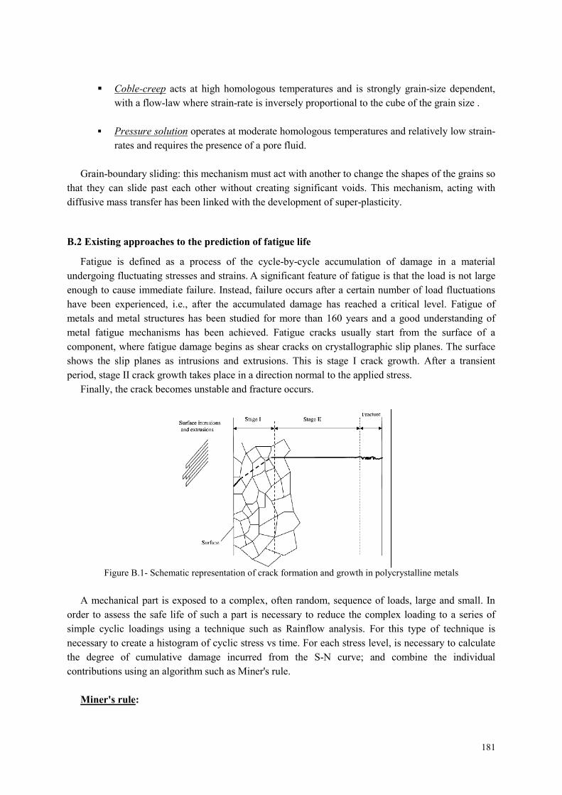
181

Coble-creep acts at high homologous temperatures and is strongly grain-size dependent,

with a flow-law where strain-rate is inversely proportional to the cube of the grain size .

Pressure solution operates at moderate homologous temperatures and relatively low strain-

rates and requires the presence of a pore fluid.

Grain-boundary sliding: this mechanism must act with another to change the shapes of the grains so

that they can slide past each other without creating significant voids. This mechanism, acting with

diffusive mass transfer has been linked with the development of super-plasticity.

B.2 Existing approaches to the prediction of fatigue life

Fatigue is defined as a process of the cycle-by-cycle accumulation of damage in a material

undergoing fluctuating stresses and strains. A significant feature of fatigue is that the load is not large

enough to cause immediate failure. Instead, failure occurs after a certain number of load fluctuations

have been experienced, i.e., after the accumulated damage has reached a critical level. Fatigue of

metals and metal structures has been studied for more than 160 years and a good understanding of

metal fatigue mechanisms has been achieved. Fatigue cracks usually start from the surface of a

component, where fatigue damage begins as shear cracks on crystallographic slip planes. The surface

shows the slip planes as intrusions and extrusions. This is stage I crack growth. After a transient

period, stage II crack growth takes place in a direction normal to the applied stress.

Finally, the crack becomes unstable and fracture occurs.

Figure B.1- Schematic representation of crack formation and growth in polycrystalline metals

A mechanical part is exposed to a complex, often random, sequence of loads, large and small. In

order to assess the safe life of such a part is necessary to reduce the complex loading to a series of

simple cyclic loadings using a technique such as Rainflow analysis. For this type of technique is

necessary to create a histogram of cyclic stress vs time. For each stress level, is necessary to calculate

the degree of cumulative damage incurred from the S-N curve; and combine the individual

contributions using an algorithm such as Miner's rule.

Miner's rule:

182

In 1945, M. A. Miner popularised a rule that had first been proposed by A. Palmgren in 1924. The

rule, variously called Miner's rule or the Palmgren-Miner linear damage hypothesis, states that where

there are k different stress magnitudes in a spectrum, Si (1 ≤ i ≤ k), each contributing ni(Si) cycles, then

if Ni(Si) is the number of cycles to failure of a constant stress reversal Si, failure occurs when:

CN

nk

i i

i 1

(1)

C is experimentally found to be between 0.7 and 2.2. Usually for design purposes, C is assumed to

be 1. This can be thought of as assessing what proportion of life is consumed by stress reversal at each

magnitude then forming a linear combination of their aggregate.

Though Miner's rule is a useful approximation in many circumstances, it has two major limitations:

It fails to recognise the probabilistic nature of fatigue and there is no simple way to relate life

predicted by the rule with the characteristics of a probability distribution.

There is sometimes an effect in the order in which the reversals occur. In some circumstances,

cycles of low stress followed by high stress cause more damage than would be predicted by the rule. It

does not consider the effect of overload or high stress, which may result in a compressive residual

stress. High stress followed by low stress may have less damage due to the presence of compressive

residual stress.

Paris’s relationship:

Anderson, Gomez and Paris derived relationships for the stage II crack growth with cycles N, in

terms of the cyclical component ΔK of the Stress Intensity Factor K:

mKCdN

da (2)

where a is the crack length and m is typically in the range 3 to 5 (for metals).

This relationship was later modified (by Forman, 1967) to make better allowance for the mean

stress, by introducing a factor depending on (1-R) where R = min. stress/max stress, in the

denominator.

Low cycle fatigue. Coffin-Manson relation:

Where the stress is high enough for plastic deformation to occur, the account in terms of stress is

less useful and the strain in the material offers a simpler description. Low-cycle fatigue is usually

characterised by the Coffin-Manson relation (published independently by L. F. Coffin in 1954 and S.

S. Manson 1953):

cf

p N22

'

(3)

183

Where:

Δεp /2 is the plastic strain amplitude

εf' is an empirical constant known as the fatigue ductility coefficient, the failure strain for a

single reversal

2N is the number of reversals to failure (N cycles)

c is an empirical constant known as the fatigue ductility exponent, commonly ranging from

-0.5 to -0.7 for metals.

184

Appendix C User-defined models implementation in FEM software -Theories

In this section it will be provided an overview of the main theories for the implementation of user-

defined material models in FEM software.

C.1 Stress-rate based theories

As macroscopic plasticity theories are usually based on a yield condition, we have to identify this

feature within the microscopic theory. The need of consistent physically based definitions for the yield

surface is here required for dynamic localizations.

In inelastic deformation, the localization of deformation into narrow bands of intense straining is

considered one of the characteristic features in metals and steel alloys. Localization for the case of

rate-independent formulation is associated with a change in the character of the governing equations.

That is, under quasi-static loading conditions the equations governing incremental equilibrium lose

ellipticity, while under dynamic loading conditions wave speeds become imaginary.

Standard boundary value problems are then ill posed; one manifestation of this is that the width of

the band of localized deformation is arbitrary narrow. As a consequence numerical solutions to

localization problems for rate-independent solids exhibit inherent mesh dependence. The minimum

width of the band of localized deformation is set by the mesh spacing. Furthermore, global quantities

such as the overall stiffness characteristics of the body depend on the mesh size used to resolve the

band of localized deformations.

Under both quasi static and dynamic loading conditions, the solutions to localization problems for

rate-independent solids permit arbitrary narrow bands of intense deformation. There is nothing in the

formulation to set a minimum width to such bands. On the other hand, in numerical solutions the

minimum width is set by the mesh spacing and key features of the solutions can be a consequence of

the discretization. This is clearly an undesirable state of affairs and stems from the character of the

continuum problem.

Stress evolution representative functional:

The development of stress integration algorithms with improved performance has received

considerable attention in the recent literature on computational plasticity and visco-plasticity.

The very efficient implementations of the implicit integration using the radial return schemes for

metals corresponding to the special case of full isotropy (both elastic and inelastic responses), enabled

by the complete reductions of the rate tensor equations to a final single/scalar nonlinear equation; e.g.

in terms of the effective stress, or equivalently the plastic multiplier or the “magnitude” of the inelastic

strain vector. In order to achieve a strong algorithmic treatment for any complex visco-plasticity

constitutive models used for large-scale deformation, the following three tasks are required (Saleeb et

al., 2000); (1) detailed study of the mathematical structure of the Visco-plastic equations, and the

corresponding integrated field of stress and internal state variables, (2) development and

185

implementation of the implicit backward-Euler stress-updating algorithm, and the associated nonlinear

iteration equation solver (e.g, Newton Raphson technique), (3) testing the convergence, stability, and

accuracy properties of the algorithms.

On the theoretical side, the general framework is developed in the specific context of the fully

implicit (backward Euler) difference scheme which is known to exhibit excellent convergence and

accuracy characteristics in large scale computations that involve large time steps, particularly with

complex anisotropic inelastic models (Ortiz and Popov, 1985). Radial return algorithm which is a

special case of the backward-Euler method is used to introduce a nonlinear scalar equation in terms of

the Visco-plastic multiplier for the case of the Consistency Visco-plastic model and in terms of the

equivalent stress for the case of Perzyna Visco-plastic model. Consistent algorithmic tangent stiffness

matrices are derived for both small and finite strain Visco-plastic models.

Plasticity constitutive equations:

Nemat-Nasser and his co-workers (1991, 1992) developed an experimental technique measuring

the flow stress of different bcc, fcc and hcp metals and alloys over a broad range of strains, strain rate,

and temperatures in uniaxial compression.

Some of their experimental results are, actually, used in this work for models evaluation and

comparisons. They also presented a constitutive model that characterizes the plastic deformation of

different metals and alloys using the thermal activation concept and assuming constant dislocation

density throughout the deformation process. That is neither the plastic strain evolution of dislocation

density nor the rate multiplication of the dislocation density evolution is considered.

There has been a significant progress made over the years in the development theories of plasticity

and visco-plasticity for the phenomenological representation of inelastic constitutive properties. In

particular, mathematical modelling of metal visco-plasticity developed based on the so-called internal

state variable formalism in the thermodynamics of irreversible processes.

A large number of specialized forms of theses modern unified Visco-plastic models (e.g. isotropic

or anisotropic, fully associative or non-associative, isothermal or non-isothermal, etc.) have been

successfully applied to different metals with different crystal structures (Coleman and Gurtin, 1967;

Lublinear, 1973; Germain et al., 1983; Lemaitre and Chaboche, 1990; Arnold and Saleeb, 1994;

Robinson and Duffy, 1990; Arnold et al.,1995; Robinson et al., 1987; Freed and Walker, 1993; Simo

and Taylor, 1985).

Equilibrium surface evolution:

Zerilli and Armstrong (1987) used equilibrium equations to describe the dislocation mechanics

concept to develop a constitutive model that accounts for strain, strain rate and temperature

dependence in a coupled manner, which can be incorporated in high rates of loading related computer

codes. Their model considers two different forms for the two different classes of metals; body centred

cubic (bcc) and face centred cubic (fcc). The rational for the differences in the two forms mainly

depends on the dislocation characteristics for each this particular structure. Bcc metals show stronger

dependence of the yield stress on temperature and strain rate while in the case of (fcc) metals the yield

186

stress is mainly affected by strain hardening. In other words, the cutting of dislocation forests is the

principal mechanism in (fcc) metals, while in bcc metals; the overcoming of Peierls-Nabarro barriers

is the principal mechanism.

These two different dislocation mechanisms of the two different metal classes will be further

investigated in the following sections. The Zerilli-Armstrong model has been derived based on the

concept of thermal activation analysis for overcoming local obstacles to dislocation motion. This

model has been widely used in many computer codes from which its material parameters are

physically interpreted. In fact, this physical interpretation of material constants becomes meaningless

if one tries to identify them from the experimental data by using a very small reference strain rate

rather than using the one corresponding to the reference dislocation velocity as been derived in the

their model. Moreover, their material parameters lose their physical meaning when they are used for

high temperature and strain rate applications which will be discussed in the following sections. It has

been shown that the Zerilli-Armstrong model as compared to the Johnson-Cook model gives slightly

better correlation with experimental results; however, none of these two models is very accurate in

describing the behaviour of metals at very large strains (Johnson and Holmquist, 1988).

C.2 Strain-rate based theories

In dynamic problems that introduce high strain rates, the dynamic yield stress is considered the

most important expression needed to characterize the material behaviour and is also used in finite

element codes. Although we are concerned with the macroscopic response of the plastic flow,

investigating the grain and atomic level of the material deformation will help us understand the failure

mechanisms for different material structures.

Accordingly, the definition of dynamic yield (flow) stress differs from metal to metal depending on

their internal crystal structure; body centred cubic (bbc), face centred cubic (fcc), hexagonal close

packing (hcp), and others. These crystal structure differences affect differently the dislocations

movement during the plastic deformation process under high strain rates loading. Each of these three

crystal structures exhibits a characteristic thermo mechanical behaviour which is associated with the

available slip systems and symmetries as well as the nature of dislocation cores. The visco-plastic

deformation of steel alloys is generally controlled by the dislocation mechanisms attributed to the

content of their compositions. The percentage of carbon in steel plays a crucial role in determining the

phase behaviour (Ferrite and Austenite) of the material over a wide range of temperatures.

Generally, the plastic flow is characterized macroscopically as a visible distortion, microscopically

as the appearance of slip systems, and atomically as a movement of dislocations. Microscopic

plasticity in metals is primarily the result of dislocation moving through the crystal lattice. The

interaction of these dislocations with the lattice and the various obstacles encountered through the

lattice determine the flow strength of the material. The motion of a dislocation through the lattice or

past an obstacle requires the surmounting of an energy barrier by a combination of applied stress and

thermal activation.

The result is that the effective shear stress required to generate an overall plastic strain rate is

intimately tied to the temperature at which the deformation occurs. Competing thermal activation

effects will influence deformations that occur at both high temperature and high strain rates. The

187

coupling of rate and temperature through dislocation kinematics indicates that the rate of thermal

softening of metals should be related to the rate of deformation. These considerations are particularly

important in the development of material models for use within simulation of high-rate phenomena,

which generally involve high temperatures because of adiabatic heating.

Residual strain evolution functions:

The modelling the dynamic flow stress of the material plastic flow at high strain rates and elevated

temperatures was the main aim of the research programmes. Studies were made in characterizing

material behaviour through both phenomenological and physically based models. Empirical equations

were initially developed with simple uniaxial stress-strain models and one-dimensional stress wave

propagation models by describing the effect of temperature and strain hardening as well as strain rate

on the flow stress.

However, for the von Mises type material, the one-dimensional models that express flow stress as a

function of strain and strain rate can be converted into the equivalent three-dimensional material

models by replacing stresses, strains, and strain rates by their equivalent invariant three-dimensional

forms.

Johnson and Cock (1983) proposed a phenomenological model that is widely used in most

computer codes for static and dynamic analyses in order to predict the behaviour of the material flow

stress at different strain rates (10−4s−1-10-5s−1) and temperatures. The main advantage of this model is

that it is relatively easy to calibrate with a minimum of experimental data in the form of stress-strain

curves at different strain rates and temperatures.

Moreover, the strain rate and temperature effects on the flow stress are uncoupled which implies

that the strain rate sensitivity is independent of temperature. This is not the case as observed in most

metals. It is rather found that the rate sensitivity increases with increasing temperature while the flow

stress decreases. For this reason was born a new branch of theories able to keep into account of these

effects (Hoge and Murkherjee, 1977)

Strain potentials based methods:

The understanding of high-strain-rate behaviour of metals is essential for the modelling and

analysis of numerous processes including high-speed machining, impact, penetration and shear

localization. Recently, considerable progress has been made in understanding the role of rate

controlling dislocation mechanisms on the temperature and strain rate dependence of the flow stress

for metals and alloys. Hoge and Murkherjee (1977) studied the effect of both temperature and strain

rates on the lower yield stress of Tantalum and proposed a model incorporating the combined

operation of the Peierls’ mechanism and dislocation drag process.

They concluded from the stress-temperature relationship and the variation of the activation volume

with stress and strain that the rate controlling mechanism for deformation could be rationalized in

terms of Peierls mechanism. This behaviour is mainly attributed to the specific crystal structure of

body cubic centred metals. Steinberg and co-workers (see for example, Steinberg and Lund, 1989)

described a constitutive model for use with hydrodynamic codes to account for the dependence of

188

shear modulus and yield strength on high strain rates, temperature, and pressure-dependent melting.

Although their model is intended to be used at high strain rates, their formulation did not specifically

include strain rate effects.

This model has been widely used in many computer codes from which its material parameters are

physically interpreted. In fact, this physical interpretation of material constants becomes meaningless

if one tries to identify them from the experimental data by using a very small reference strain rate

rather than using the one corresponding to the reference dislocation velocity as been derived in the

model. It has been shown that the Zerilli-Armstrong model as compared to the Johnson-Cook model

gives slightly better correlation with experimental results; however, none of these two models is very

accurate in describing the behaviour of metals at elevated temperatures (Johnson and Holmquist, 1988;

Abed and Voyiadjis, 2005).