Universita degli Studi di Napoli Federico II
142
UNIVERSITA' DEGLI STUDI DI NAPOLI FEDERICO II Dottorato di Ricerca in Ingegneria Informatica ed Automatica MODEL-BASED DEPENDABILITY EVALUATION OF COMPLEX CRITICAL CONTROL SYSTEMS FRANCESCO FLAMMINI TESI DI DOTTORATO DI RICERCA (XIX CICLO) NOVEMBRE 2006 Il Tutore: Prof. Antonino Mazzeo I Co-Tutori: Prof. Nicola Mazzocca, Prof. Valeria Vittorini Il Coordinatore del Dottorato: Prof. Luigi P. Cordella Dipartimento di Informatica e Sistemistica Comunità Europea Fondo Sociale Europeo A. D. MCCXXIV
Transcript of Universita degli Studi di Napoli Federico II

UNIVERSITA' DEGLI STUDI DI NAPOLI FEDERICO II
Dottorato di Ricerca in Ingegneria Informatica ed Automatica
MODEL-BASED DEPENDABILITY EVALUATION OF
COMPLEX CRITICAL CONTROL SYSTEMS
FRANCESCO FLAMMINI
TESI DI DOTTORATO DI RICERCA
(XIX CICLO)
NOVEMBRE 2006
Il Tutore:
Prof. Antonino Mazzeo
I Co-Tutori:
Prof. Nicola Mazzocca, Prof. Valeria Vittorini
Il Coordinatore del Dottorato:
Prof. Luigi P. Cordella
Dipartimento di Informatica e Sistemistica
Comunità Europea
Fondo Sociale Europeo
A. D. MCCXXIV

INDEX OF SECTIONS
2
Index of Sections
Index of Sections ___________________________________________________________ 2
Index of Figures ___________________________________________________________ 4
Index of Tables ____________________________________________________________ 6
Introduction _______________________________________________________________ 8
Chapter I ________________________________________________________________ 11
Model-Based Dependability Analysis of Critical Systems __________________________ 11
1. Context ____________________________________________________________________ 11
2. Motivation__________________________________________________________________ 16
3. State of the art in dependability evaluation of critical systems _______________________ 19 3.1. Functional analysis of critical systems ________________________________________________ 19 3.2. Multiformalism dependability prediction techniques _____________________________________ 24 3.3. Dependability evaluation of ERTMS/ETCS____________________________________________ 28
Chapter II________________________________________________________________ 29
Model-Based Techniques for the Functional Analysis of Complex Critical Systems ____ 29
1. Introduction and preliminary definitions ________________________________________ 29
2. Choice of the reference models _________________________________________________ 30 2.1. Architectural model of computer based control systems __________________________________ 31 2.2. Functional block models ___________________________________________________________ 33 2.3. State diagrams___________________________________________________________________ 34
3. Model-based static analysis of control logics______________________________________ 36 3.1. Reverse engineering ______________________________________________________________ 37 3.2. Verification of compliance _________________________________________________________ 38 3.3. Refactoring _____________________________________________________________________ 38
4. Test-case specification and reduction techniques __________________________________ 38 4.1. Logic block based reductions _______________________________________________________ 40 4.2. Reduction of influence variables_____________________________________________________ 40 4.3. Domain based reductions __________________________________________________________ 41 4.4. Incompatibility based reductions ____________________________________________________ 41 4.5. Constraint based reductions ________________________________________________________ 42 4.6. Equivalence class based reductions __________________________________________________ 42 4.7. Context specific reductions_________________________________________________________ 43
5. Automatic configuration coverage ______________________________________________ 43 5.1. Definition of abstract testing________________________________________________________ 43 5.2. Abstract testing methodology _______________________________________________________ 44
6. Implementation related activities _______________________________________________ 51 6.1. Definition and verification of expected outputs _________________________________________ 51 6.2. Simulation environments for anomaly testing of distributed systems_________________________ 52 6.3. Execution, code coverage analysis and regression testing _________________________________ 53
Chapter III _______________________________________________________________ 55
Multiformalism Dependability Evaluation of Critical Systems______________________ 55
1. Introduction ________________________________________________________________ 55
2. Implicit multiformalism: Repairable Fault Trees__________________________________ 55 2.1. Repairable systems: architectural issues _______________________________________________ 55 2.2. Repairable systems: modeling issues _________________________________________________ 56 2.3. The components of a Repairable Fault Tree ____________________________________________ 58 2.4. Extending and applying the RFT formalism____________________________________________ 58

INDEX OF SECTIONS
3
3. Explicit multiformalism in system availability evaluation___________________________ 60 3.1. Performability modelling __________________________________________________________ 62
4. Multiformalism model composition _____________________________________________ 64 4.1. Compositional issues _____________________________________________________________ 64 4.2. Connectors in OsMoSys: needed features______________________________________________ 69 4.3. Implementation of composition operators in OsMoSys ___________________________________ 75 4.4. Application of compositional operators to dependability evaluation _________________________ 79
Chapter IV _______________________________________________________________ 83
A Case-Study Application: ERTMS/ETCS______________________________________ 83
1. Introduction ________________________________________________________________ 83 1.1. Automatic Train Protection Systems _________________________________________________ 83 1.2. ERTMS/ETCS implementation of Automatic Train Protection Systems ______________________ 83 1.3. ERTMS/ETCS Reference Architecture _______________________________________________ 85 1.4. RAMS Requirements _____________________________________________________________ 87
2. Functional analyses for the safety assurance of ERTMS/ETCS ______________________ 88 2.1. Functional testing of the on-board system of ERTMS/ETCS_______________________________ 88 2.2. Model-based reverse engineering for the functional analysis of ERTMS/ETCS control logics _____ 96 2.3. Functional testing of the trackside system of ERTMS/ETCS_______________________________ 99 2.4. Abstract testing a computer based railway interlocking __________________________________ 106
3. Multiformalism analyses for the availability evaluation of ERTMS/ETCS____________ 111 3.1. Evaluating the availability of the Radio Block Center of ERTMS/ETCS against complex repair
strategies by means of Repairable Fault Trees_____________________________________________ 111 3.2. Evaluating system availability of ERTMS/ETCS by means of Fault Trees and Bayesian Networks 120 3.3. Performability evaluation of ERTMS/ETCS __________________________________________ 129
Conclusions _____________________________________________________________ 132
Glossary of Acronyms _____________________________________________________ 134
References ______________________________________________________________ 136
Acknowledgements _______________________________________________________ 142

INDEX OF FIGURES
4
Index of Figures Figure 1. General scheme of a control system.____________________________________ 11
Figure 2. The distributed multi-layered architecture of a complex real-time system. ______ 14
Figure 3. Comparison of different reliability modelling formalisms. __________________ 15
Figure 4. Different views on the context under analysis. ____________________________ 16
Figure 5. An extract of the “V” development cycle for critical control systems. _________ 17
Figure 6. Example of a possible three formalisms interaction. _______________________ 24
Figure 7. A GSPN performability model example. ________________________________ 25
Figure 8. Translation of a Fault Tree into a Bayesian Network (picture taken from [5]). ___ 27
Figure 9. General structure of a computer based control system. _____________________ 33
Figure 10. System decomposition into functional blocks. ___________________________ 34
Figure 11. Test-Case (a) and Test-Scenario (b) representations. ______________________ 35
Figure 12. Combination of scenario and input influence variables.____________________ 35
Figure 13. Three steps scheme of the modeling and verification approach: 1) reverse
engineering; 2) verification of compliance; 3) refactoring. __________________________ 37
Figure 14. Tree based generation of test-cases from influence variables. _______________ 39
Figure 15. Influence variable selection flow-chart. ________________________________ 41
Figure 16. Example of robust checking for 2 influence variables._____________________ 41
Figure 17. Equivalence class based reduction.____________________________________ 42
Figure 18. The integration between generic application and configuration data. _________ 43
Figure 19. A high level flow-chart of the abstract testing algorithm. __________________ 45
Figure 20. A possible diagnostic environment. ___________________________________ 52
Figure 21. The process of translation of a FT into a RFT: (a) RFT target model; (b) FT to
GSPN translation rules; (c) GSPN translation result; (d) GSPN Repair Box definition; (e)
Repair Box connection. _____________________________________________________ 59
Figure 22. System availability modelling. _______________________________________ 61
Figure 23. Task scheduling class diagram._______________________________________ 62
Figure 24. Star-shaped task scheduling scheme. __________________________________ 62
Figure 25. The GSPN subnet for the task scheduling scheme.________________________ 63
Figure 26. OsMoSys & Mobius comparison class-diagram: compositional issues and
integration. _______________________________________________________________ 69
Figure 27. Graphical representation of a bridge between two model classes. ____________ 71
Figure 28. Multiplicity of connection operators: (a) Bridge Metaclass; (b) m>1, n>1; (c) m=1,
n>1; (d) m>1, n=1__________________________________________________________ 72
Figure 29. A low level view of an unary composition operator. ______________________ 74
Figure 30. Sequence diagram showing the interaction between submodels of different layers.
________________________________________________________________________ 82
Figure 31. A braking curve or dynamic speed profile. _____________________________ 83
Figure 32. ERTMS Trackside (left) and on-board (right) systems. ____________________ 84
Figure 33. Architectural scheme and data flows of ERTMS/ETCS Level 2._____________ 86
Figure 34. SCMT architecture diagram._________________________________________ 89
Figure 35. Context diagram for the SCMT on-board subsystem. _____________________ 89
Figure 36. Class diagram for SCMT on-board. ___________________________________ 90
Figure 37. SCMT black-box testing. ___________________________________________ 90
Figure 38. SCMT system logic decomposition. ___________________________________ 91
Figure 39. First-level horizontal decomposition of SCMT in detail. ___________________ 92
Figure 40. Test execution pipeline. ____________________________________________ 95
Figure 41. RBC software architecture. __________________________________________ 96
Figure 42. Use case (left) and class (right) diagrams for the CTP logic process. _________ 97
Figure 43. Sequence (left) and state (right) diagrams for the CTP logic process. _________ 98
Figure 44. The trackside context diagram. ______________________________________ 100

INDEX OF FIGURES
5
Figure 45. A logic scheme of the testing environment. ____________________________ 101
Figure 46. The hardware structure of the trackside simulation environment. ___________ 103
Figure 47. A representation of the TAF procedure. _______________________________ 106
Figure 48. An IXL scheme (a) and related control software architecture (b). ___________ 109
Figure 49. A RBC centered view of ERTMS/ETCS level 2. ________________________ 111
Figure 50. Class diagram of the RBC. _________________________________________ 112
Figure 51. The RBC RFT general model. ______________________________________ 114
Figure 52. The GSPN model of the RFT._______________________________________ 115
Figure 53. RBC sensitivity to number and attendance of repair resources. _____________ 116
Figure 54. RBC sensitivity to MTTR variations. _________________________________ 118
Figure 55. Comparison of different design choices._______________________________ 119
Figure 56. ERTMS/ETCS composed hardware failure model. ______________________ 120
Figure 57. Fault Tree model of the Lineside subsystem. ___________________________ 121
Figure 58. Fault Tree model of the On-board subsystem. __________________________ 123
Figure 59. Fault Tree model of the Radio Block Center. ___________________________ 125
Figure 60. The global Bayesian Network model featuring a common mode failure. _____ 127
Figure 61. The integration of performability aspects in the overall system failure model. _ 129
Figure 62. A scheme of the GSPN performability model of the Radio Block Center. ____ 130
Figure 63. A complex multi-layered multiformalism model using composition operators. 133

INDEX OF TABLES
6
Index of Tables Table 1. Variables used in the abstract testing algorithm. ___________________________ 47
Table 2. Threats of system communications. _____________________________________ 53
Table 3. Brief explanation of technical terms and acronyms used in this chapter. ________ 85
Table 4. ERTMS/ETCS RAM requirements of interest. ____________________________ 88
Table 5. COTS reliability values. _____________________________________________ 113
Table 6. Reference parameters for repair. ______________________________________ 113
Table 7. RBC unavailability with respect to resources. ____________________________ 116
Table 8. RBC unavailability with respect to maintenance priorities.__________________ 117
Table 9. RBC unavailability with respect to on-line and off-line MTTR. ______________ 118
Table 10. RBC sensitivity to MTBF variations.__________________________________ 119
Table 11. Lineside model parameters. _________________________________________ 122
Table 12. A selection of Lineside results. ______________________________________ 122
Table 13. On-board model parameters. ________________________________________ 124
Table 14. Results of the On-board sensitivity analysis. ____________________________ 124
Table 15. On-board unavailability with respect to MTTR and number of trains. ________ 125
Table 16. Trackside model parameters. ________________________________________ 126
Table 17. RBC unavailability with respect to repair times. _________________________ 126
Table 18. Trackside unavailability with respect to the number of RBCs. ______________ 126
Table 19. Conditional Probability Table of the noisy OR gate connected to the “Top Event”.
_______________________________________________________________________ 127
Table 20. Global model parameters.___________________________________________ 128
Table 21. A selection of system level results. ___________________________________ 128

7
[…]
Made weak by time and fate, but strong in will
To strive, to seek, to find, and not to yield.
A. Tennyson, Ulysses
To my nest − mum, dad and Marco
To my ever love − Antonella
And to life, seducing life

INTRODUCTION
8
Introduction Computer systems used in critical control applications are rapidly growing in complexity,
featuring a very high number of requirements together with large, distributed and
heterogeneous architectures, both at the hardware and software levels. Their dependability
requirements are even more demanding, calling for more detailed analyses in order for the
system to be evaluated against them.
Complex systems are usually evaluated against safety requirements using simulation based
techniques, while formal methods are used to verify only limited parts of the system. When
evaluating system as a whole (i.e. as a “black-box”), the simulation techniques belong to the
class of functional testing. Traditional functional testing techniques reveal inadequate for the
verification of modern control systems, for their increased complexity and criticality
properties. Such inadequateness is the result of two factors: the first is specification
inconsistency (impacting on testing effectiveness), the second is test-case number explosion
(impacting on testing efficiency). In particular, as the complexity of the system grows up, it is
very difficult (nearly impossible) to develop a stable system requirements specification. This
is a traditional problem, which is even more critical with nowadays control systems, featuring
thousands of functional requirements and articulated architectures. Accurately revising natural
language specification only reduces the problem. Missing requirements can be added at any
time, others are continuously modified; negative requirements are usually stably missing. The
ideal thing is to have a testing approach which retains a certain independence from system
specification, more focused on the variables which influence system behavior (which do not
change as long as system architecture is kept unvaried); besides guaranteeing a higher level of
coverage, such an approach would be also effective in detecting missing requirements.
Another problem which is not addressed by traditional techniques is the impossibility to bias
the test set in order to balance test effectiveness (number of potentially discovered errors) and
efficiency (time required for the execution). Grey-box approaches allow to measure test-
effectiveness by integrating the code coverage measurement; however, a stronger integration
between static and dynamic analyses techniques is needed to enhance functional testing.
To cope with the aforementioned issues, in this thesis we present a hybrid and grey-box
functional testing technique based on influence variables and reference models (e.g. UML
class and state diagrams) which is aimed at making functional testing of critical systems both
feasible and cost-effective (in other words, with respect to traditional approaches test
coverage increases and execution time decreases). While some examples of model based
testing are referenced in the research literature, it is a matter of fact that such methods are
either too much theoretical or too much specific, missing the goal to provide a general
approach which is suitable to all classes of complex critical systems. It is no surprise that
testing remains the field of system and software engineering where the biggest gap exists
between the theory and the practice; however, it is also the most critical industrial activity in
terms of needed results, budget and time, and these are significant reasons to concentrate
research efforts on it.
While component or even subsystem level reliability can be evaluated quite easily, when
availability has to be evaluated against system level requirements for non trivial failure
modes, together with maintainability constraints, no traditional technique (Faul Trees, Markov
Chains, etc.) seems to be adequate. To cope with such issue, designers use to specify more
conservative constituent level requirements, ensuring feasibility at a higher expense.
However, more strict constituent level requirements feature two disadvantages: as first,
system level availability target is not guaranteed to be fulfilled, as it depends on non
straightforward architectural dependencies (i.e. how constituent are connected and interact
with each other); secondly, even though more strict constituent level reliability requirements
would ensure the accomplishment of global availability goals, this would imply a non
balanced allocation of costs, as developers would not be able to fine tune system reliability

INTRODUCTION
9
parameters (which is only possible by means of sensitivity analyses performed on a detailed
global model). The impossibility to correctly size reliability parameters according to structural
dependencies is very likely to take to over-dimension some components and under-dimension
some others, with a negative cost impact. A combination of techniques is therefore needed to
perform system level availability modeling of complex heterogeneous control systems,
considering both structural (i.e. hardware) and behavioral (i.e. performability) studies. While
a single highly expressive formalism (e.g. high-level Petri Nets) could be adopted to model
the entire system from an availability point of view, there are at least two issues which are
related to such choice: the first is efficiency, as the more expressive formalism usually
features more complex solving algorithms (e.g. belonging to the NP-hard class); the second is
ease of use, as the more expressive formalisms usually require a skilled modeler. The former
issue is such to impede the application of an entire class of formalisms to large systems (e.g.
for the state-space explosion problem). The explicit use of more formalisms (i.e.
multiformalism) allow modelers to fine tune the choice of the formalism to the needed
modeling power. Furthermore, implicit multiformalism allows modelers to specify new
formalisms out of existing ones, thus allowing to combine enhanced power, better efficiency
and increased ease of use (the complexity of the multiformalism solving process is hidden to
the modeler). Such a use of different formalisms must be supported by specifically developed
multiformalism support frameworks, allowing to specify, connect and solve heterogeneous
models. In this thesis we show how multiformalism approaches apply to critical control
systems for system availability evaluation purposes. We also dedicate a section to
multiformalism composition operators and their applications to the dependability modeling,
showing why they are needed for any kind of interaction between heterogeneous submodels.
While multiformalism approaches have been addressed by several research groups of the
scientific community a number of years ago, they have been usually applied to case-studies of
limited complexity in order to perform traditional analyses. In this thesis we show how to
employ multiformalism techniques in real-world industrial applications, in order to model and
evaluate dependability attributes with respect to system level failure modes.
The advantages of the new proposed methodologies are shown by applying them to real world
systems. In particular, in order to achieve a coherent and cohesed view of a real industrial
application, the case-studies are all related to a single railway control system specification: the
European Railway Traffic Management System / European Train Control System
(ERTMS/ETCS). ERTMS/ETCS is a standard specification of an innovative computer based
train control system aimed at improving performance, reliability, safety and interoperability of
European railways (in Italy, it is used in all the recently developed high-speed railway lines).
An implementation of ERTMS/ETCS is a significant example of what a complex
heterogeneous control system can be. At the best of our knowledge, no consistent study about
the dependability evaluation of ERTMS/ETCS is available in the research literature;
therefore, this thesis also serves as an innovative case-study description about ERTMS/ETCS.
Together with the theoretical studies, the results obtained in an industrial experience are
presented, which clearly underline the advantages of adopting the described techniques in the
V&V activities of a real-world system.
This thesis is organized as follows: Chapter I provides thesis motivation and state of the art of
simulative and (multi)formal dependability evaluation techniques. Existing dependability
(safety and availability) prediction techniques are briefly introduced and discussed, showing
their advantages and limitations and justifying the proposal for extensions needed to improve
their effectiveness and efficiency. Also, existing dependability studies of ERTMS/ETCS are
referenced.
Chapter II presents simulative model-based approaches for the functional validation of
complex critical systems; the aim of such approaches is to find systematic software errors
which impact on system behavior; in particular, it is shown how it is possible to combine

INTRODUCTION
10
static and dynamic analyses in order to enhance both effectiveness and efficiency of
functional testing, by means of innovative hybrid and grey-box testing techniques.
Chapter III deals with multiformalism modeling techniques for dependability evaluation,
presenting advanced implicit and explicit multiformalism methodologies and their
applications, based on the OsMoSys1 approach; in particular Repairable Fault Trees and
Bayesian Networks are introduced in order to enhance the evaluation of system level impact
of reliability and maintainability choices. Moreover, in this chapter we present the theoretical
and applicative aspects related to composition operators, which are used to make
heterogeneous models interact in a multiformalism support environment.
In Chapter IV a short architectural and behavioral description of the reference case-study (i.e.
ERTMS/ETCS) is provided. Then, several applications of dependability evaluation techniques
to different subsystems of ERTMS/ETCS are described, highlighting the results obtained in a
real industrial experience., that is to say the functional testing of ERTMS/ETCS for the new
Italian High-Speed railway lines. Several studies about the multiformalism evaluation of
ERTMS/ETCS availability are presented, showing their advantages with respect to traditional
approaches.
1 OsMoSys is a recently developed multiformalism/multisolution graphical and object-based framework.

MODEL-BASED DEPENDABILITY ANALYSIS OF CRITICAL SYSTEMS
11
Chapter I
Model-Based Dependability Analysis of Critical Systems
1. Context
Computer based control systems are nowadays employed in a variety of mission and/or safety
critical applications. The attributes of interest for such systems are known with the acronym
RAMS, which stands for Reliability Availability Maintainability Safety. The demonstration of
the RAMS attributes for critical systems is performed by means of a set of thorough
Verification & Validation (V&V) activities, regulated by international standards (see for
instance [31] and [133]). In short, to validate a system consists in answering the question “Are
we developing the right system?”, while to verify a system answers the question “Are we
developing the system right?”. V&V activities are critical both in budget and results, therefore
it is essential to develop methodologies and tools in order to minimize the time required to
make the system operational, while respecting the RAMS requirements stated by its
specification. In other words, such methodologies and tools must provide means to take to an
improvement both in effectiveness and efficiency of system development and validation
process.
Control systems are meant to interact with a real environment, reacting in reduced times to
external stimuli (see Figure 1); therefore, they are also known as reactive systems. This is the
reason why such systems are required to be real-time2, that is a possibly catastrophic failure
can occur not only if the system gives incorrect results, but also if correct results are late in
time [152].
Figure 1. General scheme of a control system.
Another feature of most control systems is that they are embedded (in opposition to “general
purpose”), that is their hardware and operating systems are application specific. The main
motivation of such a choice consists in enhanced reliability and survivability together with
shorter verification times, as system behavior is more easily predictable, being its structure
kept as simple as possible. In fact, dependability evaluation requires non straightforward both
structural and behavioral analyses.
Dependability is an attribute related to the trustworthiness of a computer system. According
to the integrated definition provided in [2], it consists of threats (faults, error, failures),
attributes (reliability, availability, maintainability, safety, integrity, confidentiality) and means
(fault prevention, tolerance, removal, forecasting). It has been introduced in recent times in
2 Critical control systems are often classified as “hard” real-time to distinguish them from “soft” real-time
systems in which there is no strict deadline, but the usefulness of results decreases with time (timeliness
requirements are less restrictive). In this thesis we generally refer to hard real-time systems.
CONTROL
SYSTEM
SENSOR
SYSTEM
ACTUATOR
SYSTEM
ENVIRONMENT

MODEL-BASED DEPENDABILITY ANALYSIS OF CRITICAL SYSTEMS
12
order to provide a useful taxonomy for any structured design and evaluation approach of
critical systems. A system is dependable if it can be justifiably trusted. Dependability threats
are related to each other: symptoms of a failure are observable at system’s interface (a service
degradation or interruption occurs); errors are alteration of system’s internal state which can
remain latent until activated and hence possibly leading to failures; faults are the causes of
errors, and they are also usually subject to a latency period before generating an error. Errors
can also be classified as casual, when they are caused by faults which are external to system
development process, or systematic, when faults are (unwillingly) injected during system
development process.
It is very useful to evaluate system dependability from early stages of system development,
i.e. when just a high level specification or a rough prototype is available, in order to avoid
design reviews and thus reduce development costs. Such early evaluation of system
dependability is often referred to as dependability prediction. Generally speaking, most of
dependability prediction techniques can be used at different stages of system development,
being as more accurate as more data is available about the system under analysis. In fact, the
same techniques are also used to evaluate the final system, in order to demonstrate (e.g. to an
external assessor) the compliance of system implementation against its requirements. When
used in early stages, dependability prediction techniques are very effective in giving an aid to
system engineers to establish design choices and fine tune performance and reliability
parameters; in fact, design reviews should be performed as soon as possible during system life
cycle, as lately discovered errors are far more costly and dangerous than early discovered
ones.
Two main approaches are employed in order to predict/evaluate the dependability of critical
control systems: the first is based on simulation based techniques, e.g. fault-injection [105]
at the hardware level (either physical or simulated) or software testing [23] at the various
abstraction and integration levels; the second is based on formal methods [49], which can be
used at any abstraction level (both hardware and software) and at any stage of system
development and validation. Simulation based techniques are aimed at approximating the
reality by means of simulative models, e.g. small scale hardware prototypes and/or general
purpose computers running software simulators, i.e. programs implementing external stimuli
as well as possibly simplified target systems. Formal methods follow for an alternative
strategy, consisting in creating and solving a sound mathematical model of the system under
analysis, or of just a part of it, using proper languages, well defined in both their syntax and
semantic. Formal methods produce a different approximation of reality, which gives more
precise and reliable results, but it is often less efficient and more difficult to manage. Graph-
based formal languages feature a more intuitive semiotic, improving the method under the
easy of use point of view. Both simulative and formal approaches are used in real world
applications, for different or same purposes, and can be classified as model-based
techniques, as they require designers to generate an accurate model both of the system under
analysis and of the external environment (i.e. interacting entities); moreover, they can be (and
often are) used in combination, with formal models possibly interacting with simulative ones
(an example of this is model-based testing [115], which however defines a class of approaches
and not a specifically usable methodology). A model is an abstraction of real entities;
therefore, it is important to ensure that it adequately reflects the behavior of the concrete
system with respect to the properties of interest (model validation and “sanity checks” are
performed at this aim).
Many standards and methodologies have been developed in order to guide engineers in
performing safety and reliability analyses of computer systems; however, they generally
suffer from one or more of the following limitations:
• They are either application specific or too general;
• The several proposed techniques are poorly cohesed;

MODEL-BASED DEPENDABILITY ANALYSIS OF CRITICAL SYSTEMS
13
• They are either not enough effective or efficient (i.e. they are not compatible with the
complexity of real industrial applications);
• Models are difficult to manage and/or the required tools are not user friendly.
Such limitations often constitute an obstacle in implementing them in the industry, where
traditional best practice techniques continue to represent the most widespread approaches.
However, as the requirements of modern control systems grow in number and criticality,
traditional techniques begin to reveal poorly effective and efficient. The increase in
requirements also reflects in highly distributed architectures, featuring enormously increased
classes of failure modes; such systems reveal very difficult to verify.
This is especially true when performing system level dependability prediction of complex
critical systems, in a verification and validation context (which means that external
constraints are given, meeting system requirements and guidelines of international standards).
A system level analysis does not replace the component based approach, in which constituent
level requirements have to be fulfilled; on the contrary, it joins and often bases on the results
of lower level analyses. The challenge stands in the fact that system level dependability
prediction is way more difficult to perform for the obvious growth in size and heterogeneity;
however, it is the only way to fulfill system level dependability requirements (this is
mandatory for safety requirements, while it can be not mandatory but convenient for
reliability requirements). A system level study requires the evaluation of two main aspects of
interest (of which we give here only intuitive definitions):
• System safety, related above all to functional aspects: system must behave correctly
(with no dangerous consequences for human beings and the environment) in any
operating condition, including degraded ones;
• System availability, related above all to structural aspects: system should be
operational for as much time as possible, also in presence of faults.
Availability and safety are often correlated according to two aspects: first, increasing system
safety level can decrease its availability, and vice versa; secondly, in many cases a poorly
available system is also an unsafe system, e.g. when availability has a direct impact on safety,
like in aerospace applications. The evaluation of both aspects requires structural as well as
behavioral analyses. An integration of techniques is needed for managing the complexity and
heterogeneity of modern computer-based control systems when evaluating their system level
dependability (in terms of safety and availability, the latter strictly related to reliability and
maintainability aspects); such integration is aimed at improving:
• Effectiveness: more (automated) analyses are possible, in order to answer as many
“what if?” (i.e. qualitative) and “how long?” (i.e. quantitative) questions as possible;
• Efficiency: already feasible analyses can be performed more quickly or can be applied
to larger systems (i.e. they scale up better);
• Easy of use: analyses can be performed by building and evaluating models in a more
intuitive and straightforward way, with positive impact on readability, reusability and
maintainability, which obviously reduce the time to market of the final product.
Performing a system level analysis requires combining a set of already existing model-based
techniques or developing entirely new ones. In order to achieve such aim, modular and
divide-et-impera approaches of modelling and analysis are necessary, possibly using bottom-
up (i.e. inductive) or top-down (i.e. deductive) composition/decomposition techniques. A
complex embedded computing system can be represented in its distributed and multi-layered
hardware and software structure as in Figure 2, in which rows represent complete subsystems
or simpler but independent devices. It usually features a single distributed hardware layer,
constituted by a set of devices interacting one with each other by means e.g. of
communication channels. Software layers are also interacting and can be assigned different
semantics, but in general they can be roughly associated to the levels of the ISO/OSI protocol
stack. Higher application layers usually implement system functional requirements and can be
further decomposable into specific sublevels for convenience of analysis. Of course, not all

MODEL-BASED DEPENDABILITY ANALYSIS OF CRITICAL SYSTEMS
14
devices of the system have to implement all levels, with simpler devices only featuring few of
them (this is one aspect of heterogeneity). Finally, each layer of each subsystem is constituted
by a varying set of interconnected components (e.g. CPU, communication interfaces, power
supply, bus, etc. for the hardware levels).
Figure 2. The distributed multi-layered architecture of a complex real-time system.
As aforementioned, system level dependability attributes of critical systems are more difficult
to predict with respect to single components, for complexity reasons. Usually verification and
validation techniques can be distinguished into two main subgroups: the ones aimed at
studying system availability (i.e. the RAM part of the RAMS acronym) and the ones aimed at
analysing system safety. In the two subgroups, both simulative and formal means of analysis
can be employed: e.g. fault injection techniques and fault tree analyses are both employed to
evaluate hardware level availability; functional testing and model-checking approaches are
used in order to evaluate software safety. However, concentrating on system level analyses, it
usually happens that for complex critical systems:
• formal techniques are suited and widespread for system-level availability prediction
(while simulative techniques based on fault-injection are used at the component level
in order to evaluate component reliability and coverage of fault-tolerance
mechanisms);
• simulation based techniques are suited and widespread for system-level safety
prediction (while formal techniques based on model-checking or theorem-proving
reveals almost always inadequate to deal with complex systems and are only used for
small subsystems).
Of course, it would be highly advantageous to perform system level safety analyses of
complex systems by means of formal methods, but this is far from industry common practice.
This notwithstanding, many of the formal methods introduced to predict system availability
can be also employed, at least partially, for qualitative or quantitative safety-analyses.
The dynamic verification (by simulation) that a system in its whole behaves as expected, that
is it respects its functional requirements (comprising safety related ones), is know as system
testing, black-box testing or functional testing [70].
Grey-box testing approaches, in their various interpretations, support functional testing in
allowing test engineers to fine tune the test-set with the aim of an effective coverage of
functionalities with the minimum effort in time. The result is a significant reduction in test-set
complexity, while maintaining or improving test-effectiveness. In fact, while the main
advantage of functional testing techniques is that they are relatively easy to implement, the
main disadvantage consists in the difficulty of balancing test effectiveness and efficiency. As
effectiveness is difficult to predict, a thorough and extensive (thus costly and time consuming)
test specification and execution process is usually performed on critical systems. Given the
high number of variables involved, the required simulations (or test-runs) are prohibitive, thus

MODEL-BASED DEPENDABILITY ANALYSIS OF CRITICAL SYSTEMS
15
the process is necessarily either unfeasible or incomplete, with possible risks on system
safety.
The need for multiformalism modelling approaches [67] is a consequence of the limitations of
a single formalism when dealing with system level evaluations. Such limitations consist in the
following:
• inadequateness of expressive power of the formalism in modelling complex structures
or behaviors;
• inadequateness of solving efficiency in dealing with complex systems (e.g. the well
known problem of the “state space explosion”);
“Applied to computer systems development, formal methods provide mathematically based
techniques that describe system properties. As such, they present a framework for
systematically specifying, developing, and verifying systems.” (citation from [86]). Formal
methods are employed in a variety of industrial applications, from microprocessor design to
software engineering and verification (see [49] for a survey of most widespread methods and
their successful applications). Despite of such variety of methods and applications, no formal
method seems suitable to represent an entire system from both a structural and functional
point of view. While it is possible to find methods with which hardware complexity can be
managed, at least when modelling dependability related aspects, extensive formal modelling
of system level functional aspects seems still unfeasible using nowadays available tools. This
is the reason why well established formal methods are largely employed in industrial context
only for reliability analyses. For instance, Fault Trees (FT) and Reliability Block Diagrams
(RBD), are quite widespread for structural system modeling [146], while some kinds of
maintainability and behavioral analyses are possible by using Continuous Time Markov
Chains (CTMC) [74] and Stochastic Petri Nets (SPN) [102]. The latter two formalisms feature
reduced efficiency due to the state-based solving algorithms and are therefore unable to model
very complex systems. The Bayesian Network (BN) formalism [52] has been successfully
applied to dependability modeling in recent times (see [51], [96] and [5]); even though its
solving algorithm are demonstrated to be NP-hard, they feature better efficiency with respect
to GSPN being non-state based [6]. A comparison between the mentioned formalisms is
provided in Figure 3.
Figure 3. Comparison of different reliability modelling formalisms.
Multiformalism approaches are very interesting for their ability to balance the expressive
power of formal modeling languages and the computational complexity of solving algorithms.
Unfortunately and despite of their huge potential, multiformalism techniques are still not
widespread in industrial practice. The main obstacles are the difficulty of use and the limited
efficiency. Moreover, the research community is far from developing a user friendly,
comprehensive and efficient framework for managing multiformalism models. Some
approaches that move toward the achievement of such an objective show the numerous
advantages in adopting multi-formal techniques for many kinds of system analyses (see e.g.
the OsMoSys [150] and Möbius [44] multiformalism frameworks). This also highlights the
necessity of developing flexible composition operators for more strict interactions between
submodels, allowing for more comprehensive and detailed analyses. A theoretical
FT, RBD
BN
CTMC,
GSPN

MODEL-BASED DEPENDABILITY ANALYSIS OF CRITICAL SYSTEMS
16
multiformalism framework based on composition operators would be advantageous in
integrating heterogeneous models (both simulative and formal) within a single cohesed view,
which could be employed in order to obtain results which are currently almost impossible to
achieve. Composition operators are therefore orthogonal to both simulative and formal safety
and availability evaluation techniques.
Figure 4 provides a synthesis of the context under analysis, by integrating different views. In
particular:
• blue links refer to multiformalism evaluation of structural availability;
• orange links refer to model-based static functional verification techniques;
• red links refer to model-based dynamic functional verification techniques;
• green links refer to performability evaluations;
• shaded rectangles represent threats, attributes and means of interest.
Black links represent other approaches, generally non suitable or advantageous for system
level analyses (e.g. fault-injection and model-checking). While it seems possible to apply
multiformalism techniques for system structural safety evaluation, this is not necessary in
most of the cases (structural safety can be evaluated using more straightforward techniques
basing on “safe” simplifying assumptions). Analogously, while functional testing can help
detecting anomalies and non conformities having impact on system availability, it cannot
prove the absence of deadlocks. The dashed red line between “specification” and “validation”
refers to the possibility of the model-based dynamic analysis techniques to also detect the
frequent natural language specification flaws, which are obviously impossible to detect using
traditional techniques only based on the informal requirements.
DEPENDABILITY
FAULTS
THREATS ERRORS
FAILURES
AVAILABILITY
ATTRIBUTES
RELIABILITY
SAFETY
CONFIDENTIALITY
INTEGRITY
MAINTAINABILITY
TOLERANCE
MEANS
PREVENTION
FORECASTING
REMOVAL
SYSTEM
FAILURESAFETY RELATED
AVAILABILITY RELATEDDUE TO CASUAL FAULTS
DUE TO SYSTEMATIC FAULTS
HARDWARE
SOFTWARE
FORMAL
SIMULATIVE BEHAVIORAL
STRUCTURAL
SPECIFICATION
DESIGN
HARDWARE
SOFTWARE
IMPLEMENTATION
VERIFICATION
VALIDATION
LIFE CYCLE VIEW
SYSTEM VIEW
DEPENDABILITY VIEW
DYNAMIC
STATIC
Figure 4. Different views on the context under analysis.
2. Motivation
This thesis provides an integration of existing techniques and proposes new approaches to
cope with system level dependability evaluation issues of complex and critical computer-
based control systems. An application of the new approaches is also shown for a modern
railway control system. In the following of this section we explain why traditional safety and
availability evaluation techniques reveal inadequate and what are the means we propose in
this thesis in order to overcome such limitations.
Computer based control systems have growth in complexity and criticality. The complexity
growth is an effect of larger, more distributed (even on large territories) and heterogeneous
architectures. Traditional techniques which have been used in the past to predict and evaluate

MODEL-BASED DEPENDABILITY ANALYSIS OF CRITICAL SYSTEMS
17
their dependability have revealed inadequate to manage such increased complexity while
retaining power of analysis and accuracy of results.
A critical computer system is needed to be above all available and safe. Availability and
safety are conditioned both by software and hardware contributions. In particular, let us refer
to an extract of a “V” development model taken from one of the RAMS standards for critical
systems [33], which is shown in Figure 5.
Figure 5. An extract of the “V” development cycle for critical control systems.
As we can see from the diagram of Figure 5, hardware and software validation are performed
in two distinct phases, and finally integration and system testing is performed. At each
validation stage, system hardware or software must be validated against safety and availability
related failure modes considering both casual and systematic errors and using simulation or
formal means of analysis. In order to manage complexity, incremental and differential
approaches are suggested by V&V standards, which allow to independently test hardware and
software, at different verification stages. According to such approaches, when evaluating
dependability attributes of system software, engineers can neglect casual errors, as hardware
inducted software errors are demonstrated to be tolerated by fault tolerance mechanisms with
a very low probability of undetected failures (typically lower than 10-9 F/h; see [13]).
From the above considerations, we can infer that, assuming a validated hardware, software
safety and availability are only related to functional correctness (e.g. absence of deadlocks).
Functional correctness at a software level is obviously necessary to assure system safety. It
can be evaluated using functional testing (a simulative approach) or model-checking (a formal
approach); however, model checking techniques are very hard to be effectively applied to
complex control systems, for they suffer from the state space explosion problem. Even if they
were applicable (at least on subsystems or protocols), they would only give a complementary
contribution in system verification, as witnessed by past experiences [77]. This is the reason
why in this thesis we stress a model-based functional analysis approach to cope with software
functional verification: the proposed semi-formal approach balances the advantages of a
formal analysis (which helps to ensure correctness) and the flexibility of informal ones. The
functional analysis can be both static and dynamic: static analysis does not need software
execution, while dynamic analysis requires simulation. The model-based static and dynamic
analysis techniques proposed in this thesis help finding more errors more quickly with respect
to traditional techniques, e.g. only based on code inspection and black-box testing. Both
types of functional analysis share the goal of finding software systematic errors (also known
as “defects”). The proposed model-based functional analysis process involves several
activities traditionally related to functional (or system) testing and features the following
original contributions:
• the construction of reference models, that guide test engineers throughout the
functional analysis process;

MODEL-BASED DEPENDABILITY ANALYSIS OF CRITICAL SYSTEMS
18
• the static verification and refactoring techniques, based on reverse engineering and on
the Unified Modeling Language;
• the definition and reduction techniques of the input and state variables influencing
system behavior in each operating scenario;
• the test-case reduction rules, some of which are based on the functional decomposition
of the system under test;
• the abstract testing approach, which allows for a configuration independent test
specification and an automatic configuration coverage by means of the proposed
instantiation algorithm.
These features make the proposed methodology:
• model-based, as models of the system under verification are needed to support the
functional analysis process;
• hybrid, as besides verifying system implementation, its specification is also partly
validated by means of model-based analyses (missing and ambiguous requirements
can be easily detected);
• grey-box, as it needs to access system internal status for the software architecture
analysis and for logging of the variables of interest;
• abstract, as test specification results are not linked to a particular installation of the
control system.
The functional analysis methodology introduced above is described in Chapter II.
As mentioned above, the hardware validation against safety is based on well established
techniques, meant to reduce to a largely acceptable level the probability of occurrence of
unsafe hardware failures. As unsafe failure modes are quite easy to be defined and combined,
system level safety analyses are feasible with usual techniques (e.g. Fault Tree Analysis)
basing on “safe” simplifying assumptions. The hardware validation against availability is
instead problematic at a system level when non trivial failure modes are defined, each one
requiring specific analyses. The choice of using more reliable components, which is
sometimes possible by respecting constituent level reliability requirements, can not be
considered as satisfactory, as cost would increase uncontrollably and the overall system
availability with respect to a certain failure mode would be still undefined. Moreover, even
though hardware is reliable, it is not guaranteed to be performable enough, hence timing
failures can still occur. Therefore, the risk is to either oversize components or overestimate
system availability. When data of measurements from real system installation is available, it
could be too late or too costly to modify design choices. Therefore, predicting system
hardware availability from early design stages is very important. However, traditional
modeling techniques are either too weak in expressive power or poorly efficient to be
employed for a system level analysis, especially when taking into account components
dependencies (e.g. common modes of failure) and articulated maintainability policies. A
multiformalism approach, allowing to fine tune effectiveness and efficiency while modeling
the overall system by different formalisms, is the solution we propose in this thesis to cope
with the problem of hardware availability prediction.
Composition operators are needed for a more strict interaction between submodels in explicit
multiformalism applications. A highly cohesed system-level model, which is only possible
using composition operators, allows for any kind of analyses (e.g. “what if?”), both functional
and structural (e.g. to evaluate system level impact of component related parameters or design
choices); therefore such operators are orthogonal to both simulative and formal model-based
techniques, both for safety and availability evaluation. This is the reason why we perform in
this thesis a study of multiformalism composition operators, referring in particular to a
possible implementation in the OsMoSys framework. While all multiformalism frameworks
provide the possibility of implementing some kinds of model connection, no study has been
performed to exhaustively present the issues related to composition operators (e.g. needed

MODEL-BASED DEPENDABILITY ANALYSIS OF CRITICAL SYSTEMS
19
features, attributes, preservation of properties, etc.); furthermore, composition operators have
not been extensively addressed in the OsMoSys framework yet. An integration of such
operators in the already existing OsMoSys multiformalism multi-solution framework is then
proposed in this thesis, by exploiting the specific features of a graph-based object oriented
architecture and user interface. However, we do not dare to overcome all the difficulties when
trying to check properties on large composite models, which is one of the most challenging
among still open problems in the formal methods research community. The solution of such
models itself constitutes a non straightforward problem which we address. Multiformalism
dependability evaluation is discussed in Chapter III of this thesis.
The methodological contributions presented in this thesis have all been validated by applying
them to the same case-study, which is complex enough to provide plenty of possible analyses,
both from structural and behavioral points of view. In particular, the case-study consists in the
European Railway Traffic Management System / European Train Control System
(ERTMS/ETCS), a European standard aimed at improving performance, reliability, safety and
interoperability of transeuropean railways [147] which is used in Italy on High Speed railway
lines (the “Alta Velocità” system). ERTMS/ETCS specifies a complex distributed railway
control system featuring strict safety and availability requirements. One of the innovations of
this thesis is the presentation of useful results about how to perform system testing and how to
size reliability and maintainability parameters of an ERTMS/ETCS implementation. Without
the methodologies presented in this thesis, such complex system would have been almost
impossible to validate, for the difficulty of managing its complexity when assessing its system
level safety and availability using traditional approaches. These results, which are all original
contributions, are provided in Chapter IV.
3. State of the art in dependability evaluation of critical systems
As stated in previous chapter, the use of differential and incremental approaches appears to be
the only way to manage complexity and criticality of modern control systems. We recall that
the approach followed in this thesis is based on the separation of concerns between:
a. System level functional analysis, for the detection of software systematic errors
possibly impacting on system safety;
b. Evaluation of system level RAM attributes, with respect to failure modes due to casual
hardware faults or performance degradations.
Point (a) is addressed in this thesis by using model-based static and dynamic functional
analysis approaches, while point (b) is addressed by means of multiformalism techniques; in
this section we then divide our state of the art discussion between such two aspects,
respectively discussed in next subsections §3.1 and §3.2.
3.1. Functional analysis of critical systems
Functional analysis of critical systems is the both static and dynamic activity aimed at
detecting systematic software errors. Besides module testing, which is usually performed in
the downstream phase of the “V” life-cycle diagram, two main activities are widespread in
industrial V&V practice:
• Code inspection (a static analysis technique)
• Functional testing (a dynamic analysis technique)
The first activity is also known as code review or walkthrough and is usually based on
checklists [16]. Its aim is to reveal misuse of code statements and detect errors which are
evident from a static analysis of code structure. Such activity is important not only to perform
a gross grain error detection, but also to find code defects which always remain undetected
during the following dynamic analysis stage. In fact, the limited execution time of system
tests often is unable to reveal latent errors due to wrong assignment of values to variables or
pointers. However, static analysis of software could be much more effective, as often errors
are revealed in the following dynamic analysis stage that could have been detected by means

MODEL-BASED DEPENDABILITY ANALYSIS OF CRITICAL SYSTEMS
20
of a more accurate static analysis. Of course, lately discovered errors are more costly and
difficult to correct. A way to improve code inspection both in effectiveness and efficiency to
substitute it with a model-based static analysis approach, which can be also used for high
level behavioral analyses and code improvements, as we will see later in this chapter.
The second activity is also known as black-box testing and is related to the dynamic analysis
stage, where software is usually executed on the target hardware system.
Two main challenging issues have to be faced when functional testing safety-critical systems:
• Management of criticality (related to test effectiveness);
• Management of complexity (related to test efficiency).
Criticality is related to the fact that functional testing is one of the last activities to be
performed before system is put in exercise, and thus it must ensure the overall trustworthiness
of system operation. For the same reason, it also the activity which is more time critical, as a
delay in performing functional testing directly impacts on the time to market of the product.
Therefore, both a safety and budget criticality exist, and this especially true for large
heterogeneous systems, which are very hard to test extensively, but at the same time are more
error prone due to their inner complexity. Once more, we just highlighted that a balanced
compromise between test effectiveness and efficiency is necessary.
As largely mentioned in previous chapter, the functional verification of critical systems
require a thorough set of testing activities. The verification of system implementation against
its functional requirements is usually pursued by means of black-box testing approaches
[152]. Like any system level verification activity, black-box testing is inherently complex,
given the high number of variables involved. To cope with test-case explosion problems,
several techniques have been proposed in the research literature and successfully applied in
industrial contexts. Partition testing [22] is the most widespread functional testing technique.
It consists in dividing the input domain of the target system into properly chosen subsets and
selecting only a test-case for each of them. Equivalence partitioning, cause-effect graphing
[70], category-partition testing [144] and classification-tree method [104] are all
specializations of the partition testing technique.
The main limitation of “pure” black-box testing is the lack of the possibility to measure test
effectiveness. In fact, it can be proven that exhaustive black-box testing is impossible to
achieve with no information about system implementation [70]. Test adequacy can only be
assessed by means of empirical techniques, e.g. when errors/test curve flattens out. This is
why grey-box approaches are necessary for critical systems. Another important though often
neglected limitation is that black-box testing approaches are based on system specification,
which is usually expressed in natural language, besides being destined to be corrected,
integrated and refined several times during system life cycle. Therefore, its completeness and
coherence are far to be guaranteed, and this is especially true for complex systems. The use of
formal specification methods is unfeasible (at least at system level) for complex systems,
despite of the remarkable efforts of the research community. As a matter of fact, testing is the
area of software engineering showing the greatest gap between theory and practice, and this is
a very significant statement. There are several reasons impeding the system level use of
formal specification languages, among which:
• Translating system specification into a formal language requires skill, is time-
consuming and costly both to perform and to maintain (given the instability of
requirements), even using intuitive languages (like UML);
• Applying verification techniques on such a formal specification can be unfeasible due
to the impossibility to manage the complexity level (the efficiency of model-checkers
is quite limited).
Therefore, it is easy to conclude that the effort is hardly repaid. The alternative approach is to
improve the traditional informal techniques, which have several margins of enhancement, and
this is the way we choose to follow in this thesis work. Empirical observations of industrial
testing lead to the generally accepted consideration that no single technique is sufficient to

MODEL-BASED DEPENDABILITY ANALYSIS OF CRITICAL SYSTEMS
21
verify and validate software. Any technique must be assessed by considering its strengths and
weaknesses, together with incremental and integration issues. Therefore, a complete
functional testing process should be: grey-box based, requiring test-engineers to access
system internal structure (i.e. software architecture and system state); hybrid, integrating a
series of different partly existing and partly newly developed approaches (e.g. model-based
testing and equivalence class partitioning).
3.1.1 Grey-box testing
Generally speaking, grey-box means any combination of black and white box testing.
However, in traditional approaches, grey-box only refers to functional testing with added code
coverage measures. Code coverage analysis is a structural testing technique. Structural testing
compares test program behavior against the apparent intention of the source code. This
contrasts with functional testing, which compares test program behavior against a
requirements specification. Structural testing examines how the program works, taking into
account possible pitfalls in the structure and logic. Functional testing examines what the
program accomplishes, without regard to how it works internally. Structural testing is also
called path testing since test cases are selected that cause paths to be taken through the
structure of the program. At first glance, structural testing seems unsafe as it cannot find
omission errors. However, requirements specifications sometimes do not exist, and are rarely
complete. This is especially true near the end of the product development time line, when the
requirements specification is updated less frequently and the product itself begins to take over
the role of the specification; therefore, the difference between functional and structural testing
blurs near release time.
Code coverage analysis is the process of:
• Detecting code areas of a program not exercised by the test suite;
• Specifying additional test cases to increase coverage;
• Determining a quantitative measure of test effectiveness, which is an indirect quality
measure.
An optional aspect of code coverage analysis is the identification of redundant test cases that
do not increase coverage. A code coverage analyzer automates this process. Coverage
analysis requires access to source code, for instrumentation and recompilation.
A large variety of coverage measures exist. In the following, we present a survey of them
(refer to [23], [118] and [132] for further reading).
• Line (or statement) Coverage. This measure reports whether each executable statement
is encountered. Advantage: it can be applied directly to object code and does not
require processing source code. Disadvantage: it is insensitive to decisions (control
structures, logical operators, etc.).
• Decision (or branch) Coverage. This measure reports whether boolean expressions
tested in control structures are evaluated to both true and false. The entire boolean
expression is considered one true-or-false predicate regardless of whether it contains
logical-and or logical-or operators; additionally, this measure includes coverage of
“switch” statement cases, exception handlers, and interrupt handlers. Advantage:
simplicity, without the problems of statement coverage. Disadvantage: it ignores
branches within boolean expressions which occur due to short-circuit operators (e.g.
“if (condition1 && (condition2 || function1()))” ).
• Condition Coverage. Condition coverage reports the true or false outcome of each
boolean sub-expression, independently of each other. This measure is similar to
decision coverage but has better sensitivity to the control flow. Multiple condition
coverage reports whether every possible combination of boolean sub-expressions
occurs. However, full condition coverage does not guarantee full decision coverage.

MODEL-BASED DEPENDABILITY ANALYSIS OF CRITICAL SYSTEMS
22
• Condition/Decision Coverage. It is a hybrid measure composed by the union of
condition coverage and decision coverage. It has the advantage of simplicity but
without the shortcomings of its component measures.
• Path (or predicate) Coverage. This measure reports whether each of the possible paths
in each function have been followed. A path is a unique sequence of branches from the
function entry to the exit. Since loops introduce an unbounded number of paths, this
measure considers only a limited number of looping possibilities. A large number of
variations of this measure exist to cope with loops, basing on the number of
repetitions/iterations. Path coverage has the advantage of requiring very thorough
testing. Path coverage has two severe disadvantages. The first is that the number of
paths is exponential to the number of branches. The second disadvantage is that many
paths are impossible to exercise due to relationships of data.
• Data Flow Coverage. This variation of path coverage considers only the sub-paths
from variable assignments to subsequent references of the variables. The advantage of
this measure is the paths reported have direct relevance to the way the program
handles data. One disadvantage is that this measure does not include decision
coverage. Another disadvantage is complexity. Researchers have proposed numerous
variations, all of which increase the complexity of this measure. As with data flow
analysis for code optimization, pointers also present problems.
It is useful to compare different coverage measures: weaker measures are included in stronger
ones; however, they cannot be compared quantitatively. We list the following important
results:
• Decision coverage includes statement coverage, since exercising every branch must
lead to exercising every statement;
• Condition/decision coverage includes decision coverage and condition coverage, by
definition;
• Path coverage includes decision coverage;
• Predicate coverage includes path coverage and multiple condition coverage, as well as
most other measures.
Using statement coverage, decision coverage, or condition/decision coverage, the objective of
test engineers is about 80%-90% coverage or more before releasing. A lot of effort is needed
attaining coverage approaching 100%; the same effort might find more faults in a different
testing activity, such as formal technical review. Moreover, defensive programming structures
exist, which are hardly exercised by system tests. Therefore, a general rule consists in
reaching a high percentage of coverage for critical software (never less than 80%), while
inspecting the uncovered pieces of software in order to verify whether further testing is
needed or it is possible to justify by other means the missing coverage. In such way, the
totality of source code is either covered by tests or checked by hand (for instance, the latter is
useful in case of numerous repetitions of the same managing routines, simply “cut and pasted”
in different pieces of code).
With grey-box we also mean any access to the internal state of the system, both statically and
dynamically. With “static” we mean software architectural analysis (code structure views,
function call graphs, block models, UML diagrams, etc.), in order to:
• Detect functional dependencies and discover common code structures (e.g.
management routines) in order to apply architecture based reduction rules for
functional tests;
• Locate the logic variables to be monitored (and thus logged) when verifying system
state, which also constitute both the input and the output of a test-case;
• Aid the diagnosis and correction of detected errors.
With “dynamic” we mean on-line hardware and software diagnostics needed to access the
value of internal state variables which are not directly accessible at system’s interface. System
diagnostics should be less intrusive as possible, in order not to modify system behavior and

MODEL-BASED DEPENDABILITY ANALYSIS OF CRITICAL SYSTEMS
23
real-time properties. The ideal thing is to log all necessary state variables using the Juridical
(or Legal) recording unit (JRU or LRU) which is active during system operational life. I such
a way, system is tested together with its diagnostic extensions and therefore the risk of having
tested a different software version (featuring instrumented code) is avoided. With respect to
ad-hoc logging (only for testing purposes), this has the potential disadvantage of increasing
the size of log files; however, it is possible to implement a mechanism to select the variables
to be logged, so that during system operational life just a subset of them can be recorded
(according to JRU/LRU specification).
3.1.2 Equivalence class partitioning
An equivalence class represents a set of valid or invalid states for a condition on input
variables. The domain of input data is partitioned in equivalence classes such that if the output
is correct for a test-case corresponding to an input class, then it can be reasonably deducted
that it is correct for any test-case of that class. SECT is the acronym of “Strong Equivalence
Class Testing”, which represents the verification of system behavior against all kinds of class
interactions (it can be extended with robustness checking by also considering non valid input
classes).
For numerical variables, equivalence classes are defined by selecting a subset of their domain.
Widespread approaches include:
• “Boundary Analysis”, in which boundary values are chosen for each variability range
referred in system requirements;
• “Robustness Testing”, in which variables are assigned values external to their nominal
domain in order to check system robustness (the so called “negative tests”);
• “Worst Case Testing” (WCT) techniques, based on a combination of boundary or
robustness approaches for more than one variable at a time (e.g. all variables are set
out-of-range values).
Such techniques are based on empirical studies. For instance, it has been noted that most
errors generate in correspondence of extreme values of input variables.
3.1.3 Simulation environments
Simulation environments are needed to perform any type of dynamic analysis. Simulation3
allows for different levels of testing on (sub)system prototypes. Even when the system has
been entirely developed, simulation is still needed to speed-up testing (with respect to on-the-
field execution) and to perform negative testing whenever abnormal testing conditions are
unfeasible on the real installation for safety-reasons. When relying on simulation, testing
objectives must be clear in order to accurately select the part of the system to be simulated.
Usually, the target system is inserted into a simulated environment, providing its external
stimuli and probing its outputs, according to the classical “system-in-the-loop” scheme.
However, when hardware-software integration is not object of testing, then the target software
can be executed by means of a simulated platform running on a commercial PC. This is the
case of logic testing or preliminary software tests. In the latter case, preliminary software
versions are executed on a simulated hardware platform, in order to quickly detect the
majority of bugs. Then, when approaching the final version, software is tested using the target
hardware, in order to safely check also HW-SW integration (which is mandatory for final
system tests). System acceptance testing require that a proper subset of the entire functional
test-suite is repeated on the field. Such a subset is usually chosen with the objective of a broad
system requirements’ coverage, at least in nominal conditions. Usually, as some negative tests
related to safety critical conditions will never be executed on the real environment, the
3 An introduction to (discrete event) simulation is provided in [108], which also give references for further
readings.

MODEL-BASED DEPENDABILITY ANALYSIS OF CRITICAL SYSTEMS
24
simulation environment must be validated against the real environment, and this is performed
by observing and comparing the results of test samples.
Nominal simulation environments for the so called “engineering tests” are usually unable to
simulate all abnormal conditions required for negative testing. External tools and/or code
instrumentation is usually required to cope with the needs of extensive V&V testing (e.g. loss
of messages), as described in the following Section 6.
3.2. Multiformalism dependability prediction techniques
Multiformalism refers to the use of more variously interacting models specified in different
formal languages (see e.g. Figure 6). It helps modeling complex heterogeneous systems by
using:
• the most suited formal language for each subsystem or abstraction layer to be
modeled;
• different views on the system, according to the modeling and evaluation objectives.
The choice of “most suited” formalism depends on the needed modeling and evaluation
power, and it is the result of a trade off between effectiveness (i.e. expressive power),
efficiency (i.e. computational complexity of the solving algorithms) and ease of use.
Multiformalism techniques must be supported by proper frameworks, which should provide a
theoretical basis, covering methodological aspects, as well as integrated software toolsets for
the practical implementation and solution of multiformalism models.
Figure 6. Example of a possible three formalisms interaction.
As an example, performability models [91] are advantageously expressed through
multiformalism. Imagine a Queuing Network (QN) model representing the performance part,
and a Fault Tree representing the hardware availability part: the overall system will operate
correctly when it is available and respecting its real time requirements. Therefore, an
interaction between the two models is required, by exchanging results. Stronger interaction
would be required if modeling, for instance, the correlation between component stress factor,
due to system overhead, and its reliability. Connection and composition techniques of
heterogeneous models have been addressed in several research works; for instance, reference
[73] provides a theoretical analysis of compositional modeling with the aim of preserving
model properties. The Möbius framework [44] also provides heterogeneous model interaction
by means of composition operators, which have been already implemented. In Chapter III we
will abstract advantages and limitations of the existing approaches of model composition in
more details.
The translation of heterogeneous models into a single more powerful language is a possibility;
however, the drawbacks are graphical expressivity (model is more cryptic, that is difficult to
understand) and efficiency (the simpler submodels could be solved by means of more efficient
algorithms). As an example, consider the model of Figure 7, in which the aforementioned
multi-formalism performability example is described by means of a single formalism (GSPN);
note that the upper part models a queue, while the lower part translates quite intuitively a two
states Markov chain.
A
B
C
BE2
D
: .
BE1
TE
OR
Fault Tree Petri Net Bayesian Network
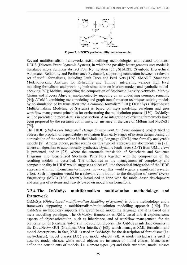
MODEL-BASED DEPENDABILITY ANALYSIS OF CRITICAL SYSTEMS
25
Figure 7. A GSPN performability model example.
Several multiformalism frameworks exist, defining methodologies and related toolboxes:
DEDS (Discrete Event Dynamic System), in which the possibly heterogeneous user model is
translated into a common abstract Petri Net notation [53]; SHARPE (Symbolic Hierarchical
Automated Reliability and Performance Evaluator), supporting connection between a relevant
set of useful formalisms, including Fault Trees and Petri Nets [129]; SMART (Stochastic
Model-checking Analyzer for Reliability and Timing), integrating various high level
modeling formalisms and providing both simulation on Markov models and symbolic model-
checking [63]; Möbius, supporting the composition of Stochastic Activity Networks, Markov
Chains and Process Algebra, implemented by mapping on an underlying common semantic
[44]; AToM3, combining meta-modeling and graph transformation techniques solving models
by co-simulation or by translation into a common formalism [101]; OsMoSys (Object-based
Multiformalism Modeling of Systems) is based on meta modeling paradigm and uses
workflow management principles for orchestrating the multisolution process [150]. OsMoSys
will be presented in more details in next section. Also integration of existing frameworks have
been proposed by the research community, for instance in the case of Möbius and MoDeST
[75].
The HIDE (High-Level Integrated Design Environment for Dependability) project tried to
address the problem of dependability evaluation from early stages of system design basing on
a translation of the views of the Unified Modeling Language (UML) into formally analyzable
models [8]. Among others, partial results on this type of approach are documented in [71],
where an algorithm to automatically synthesize Dynamic Fault Trees (DFT) from UML views
is presented, and in [25], where the automatic translation of Statecharts and Sequence
Diagrams into Generalized Stochastic Petri Nets together with the composition of the
resulting models is described. The difficulties in the management of complexity and
compositionality in HIDE would suggest as successful the theoretical integration of the HIDE
approach with multiformalism techniques; however, this would require a significant research
effort. Such integration would be a relevant contribution to the discipline of Model Driven
Engineering (MDE) [136], recently introduced to cope with the model-based development
and analysis of systems and heavily based on model transformations.
3.2.4 The OsMoSys multiformalism multisolution methodology and
framework
OsMoSys (Object-based multiformalism Modeling of Systems) is both a methodology and a
framework supporting a multiformalism/multi-solution modelling approach [150]. The
OsMoSys methodology supports any graph based modelling language and it is based on a
meta modelling paradigm. The OsMoSys framework is XML based and it exploits some
aspects of object-orientation, such as inheritance, and of workflow management, for the
orchestration of (existing) solvers in the solution process. The OsMoSys interface consists in
the DrawNet++ GUI (Graphical User Interface) [68], which manages XML formalism and
model descriptions. In fact, XML is used in OsMoSys for the description of formalisms (i.e.
meta-classes), model classes (MC) and model objects (M). A model metaclass is used to
describe model classes, while model objects are instances of model classes. Metaclasses
define the constituents of models, i.e. element types (et) and their attributes; model classes

MODEL-BASED DEPENDABILITY ANALYSIS OF CRITICAL SYSTEMS
26
define the structure of models; finally, model objects define the values of model attributes, by
instantiating model elements (e).
OsMoSys allows for two types of multiformalism:
• Implicit multiformalism, in which the modeler uses a single formalism, but the
framework manages more formalisms/solvers in order to produce the solution of the
model (this is the case of Repairable Fault Trees);
• Explicit multiformalism, in which more models written in different formal languages
interact to form the overall model (this is the case of connected/composed models).
The software architecture of OsMoSys is composed by the following entities:
• A Graphical User Interface (GUI), DrawNet++ [68], acting as an easy to use front-end
to manage model construction and solution;
• A Workflow Engine (WFE), which manages the solving process by orchestrating
heterogeneous solvers, using workflow management principles (see [57]);
• Adapters, which are used to interface with solvers and have to be designed specifically
for any solver interface.
Reference [103] provides an overview of the OsMoSys language systems (mostly XML
based). In [59] a case-study application of the OsMoSys methodology is presented, dealing
with a performability model of a RAID disk array.
3.2.5 Repairable Fault Trees
The Repairable Fault Tree (RFT) formalism [37] is an example of implicit multiformalism in
the OsMoSys framework. RFT extends the FT formalism by adding repair boxes (RB), which
model maintenance facilities of any kind, relying on the underlying powerful GSPN
formalism. This allows for the evaluation of complex repair strategies, which can only be
modeled by means of CTMC, which are however much more difficult to use with respect to
RFT, besides featuring worse efficiency. In fact, RFT are solved by means of an iterative
process, from tree leaves (i.e. basic events) upward. This allows for a better management of
complexity, as small subtrees are iteratively solved by translating them into:
• Fault trees, if they do not feature repair facilities (i.e. they are not connected to RB);
• GSPN, if they are connected to RB.
In summary, the RFT formalism tries to combine the advantages of Fault Trees in terms of
efficiency and ease of use, with the ones of GSPN in terms of expressive power.
In order to solve RFT, OsMoSys orchestrates two different solvers:
• GreatSPN [62], for the GSPN part,
• SHARPE , for the FT part.
RFT will be analyzed in more detail in Chapter III, by studying their application to repairable
systems and the formalism extension possibilities to cope with real-world repair policies.
3.2.6 Application of Bayesian Networks to dependability
Bayesian Networks (BN) is one of the formalisms used to model uncertainty by means of
statistical inference based on conditional probability relations between stochastic variables.
The interest of the dependability research community in BN is justified by their possibility of
providing software reliability estimation models as well as structural reliability analyses: an
example of the former application is provided in the ENEA ISA-EUNET Safety-Case
assessment support for the quantitative evaluation of Safety Integrity Levels (SIL) [51] (see
also [96]); the latter application is instead a consequence of the fact that a Fault Tree can be
translated into a Bayesian Network using the conversion rules reported in Figure 8 [5]. After
translation, it can be extended exploiting the greater modeling power of BN, supporting
among other things:
• Multi state events, allowing multiple failure mode modeling;
• Complex dependencies, allowing common mode failure modeling;

MODEL-BASED DEPENDABILITY ANALYSIS OF CRITICAL SYSTEMS
27
• Noisy gates, giving to modelers more possibilities with respect to basic Boolean
connectors.
BN can also be extended using dynamic [137] and decision extensions. Decision Networks
(also known as Influence Diagrams) allow to evaluate system-level cost-benefit design trade-
offs. The power of analysis of BN can be augmented using decisional extensions, namely
decision and utility nodes (see e.g. [154] for a framework proposal for multi-criteria decision
making). Decision extensions can be exploited to perform automated cost-benefit analyses on
input reliability parameters of the model (e.g. MTBF, redundancy level, etc.). This is
important because system cost raises with components’ number (linearly) and reliability
(exponentially), while benefits include system performance and availability. More complex
dependencies arise if we consider the impact of maintenance costs, which are obviously lower
for a system with a limited number of more reliable components (at equal availability).
While component level costs, e.g. due to redundancy or presence of spares, are easily
predictable, system level impact of component level reliability or replication, which is the
measure of interest, is not easy to associate to such costs. In fact, while several formalisms
exist to evaluate system level impact of components’ reliability, many of which are used in
this thesis work, none of them allows taking decision about what are the most economically
advantageous investment to perform. Furthermore, using decision nodes the number of
redundant component can be easily varied, constituting a parameter of the model which can
be used to bias design choices.
Figure 8. Translation of a Fault Tree into a Bayesian Network (picture taken from [5]).
3.2.7 Multiformalism composition operators
Multiformalism composition operators are needed for the building of highly cohesed and
comprehensive heterogeneous models, in order to make feasible, effective and efficient
system-level dependability analyses of critical apparels. Intuitively, a multiformalism
composition operator is needed to make two possibly heterogeneous models interact in some
way. The entity usually defined as a connector (or connection operator) can be considered a
weaker composition operator, as it only allows to exchange the results of the isolated solution
of submodels, which is a subset of the possible interaction between formalisms. Several forms
of connection are defined in any of the existing multiformalism modeling frameworks
(SHARPE, SMART, DEDS, etc.). They usually differ in syntactical and implementation

MODEL-BASED DEPENDABILITY ANALYSIS OF CRITICAL SYSTEMS
28
aspects, but the semantic is similar. At the state of the art, only the Möbius framework allows
both for connection and composition operators in multiformalism model interaction [44];
however, only state/event sharing based composition is allowed and only for DEDS
formalisms. OsMoSys adds the support for the elaboration of the exchanged results, besides
the simple copy, and for the superposition of homogeneous submodels, e.g. expressed through
Stochastic Well-formed Nets (see [72]). Much work is still needed to make composition
operators both powerful and user-friendly. The OsMoSys framework is a good candidate to
reach these goals, for it can act as a GUI based front-end, possibly integrating and
orchestrating the solving engine of other frameworks (like Möbius) by means of its Work
Flow Engine and Adapter layers. This allows to add power of analysis while retaining the
possibility of implementing an object based composition and an intuitive user interface for
defining and composing models. The easy extensibility of the framework, due to the
formalism description language and the solver adaptation capabilities, guarantees the
necessary flexibility in the integration of new formalisms, solvers and composition operators.
3.3. Dependability evaluation of ERTMS/ETCS
The European Railway Traffic Management System / European Train Control System
(ERTMS/ETCS) [147] was object of analysis by several research groups, both from
companies and universities. Its RAMS requirements have been standardized in [149]. An
hazard-analysis of ERTMS/ETCS is documented in [121]. Shortly after the definition of the
standard, it was tried to model and validate its specification by means of Colored Petri Nets
(see [93]), using a layered modeling approach which however was not enough to manage
system level complexity. Other unsuccessful attempts to perform formal development and
verification at the overall system level are documented in [10]. The use of model-checking
methods have taken to some results in the formal verification of the EURORADIO safety-
critical protocol of ERTMS/ETCS [127]. Other forms of model-checking using the Promela
language and the SPIN checker have proven to be a promising approach for railway
interlockings, but still not mature enough to manage real-world complexity [11].
In [15], Generalized Stochastic Petri Net models have been employed in order to model and
evaluate communication degradations due to the GSM-R network. At the best of our
knowledge, no system level hardware availability study has been performed on
ERTMS/ETCS.
As for the functional testing, a subset of ERTMS/ETCS specification suite was initially
proposed in order to support the specification of interoperability system tests [148]. It was
found that such subset was incomplete and too much requirements based, failing to provide an
extensive functional test specification aimed at ensuring system correct behavior in any
operating scenario (including the ones possibly not covered by system specification). A
reference ERTMS/ETCS subset for system testing is still missing, hence each company is
responsible for the verification of its own system implementation against safety and
interoperability requirements (a third party assessment is obviously required as with any
safety-critical railway control system [33]).

MODEL-BASED TECHNIQUES FOR THE FUNCTIONAL ANALYSIS OF COMPLEX CRITICAL SYSTEMS
29
Chapter II
Model-Based Techniques for the Functional Analysis of Complex Critical Systems
1. Introduction and preliminary definitions
In this section we present a methodology which combines static and dynamic techniques in
order to enhance the functional analysis of safety-critical systems, featuring several
advantages with respect to traditional approaches. Such a methodology is well structured,
covers all the steps of the functional testing process and revealed both effective (with respect
to traditional error prone approaches) and efficient (it allowed an easy management of
complexity) when employed in an industrial context (see Chapter IV for related case studies).
The novelty of the methodology consists in the following main original aspects:
• The definition of a cohesed functional testing process, integrating more techniques at
different levels;
• The model-based approach for test enhancement, aiding specification, test-suite
reduction and error correction;
• The introduction of system-level state-based testing, allowing for an easy manageable
and systematic approach to complex systems’ testing;
• The use of influence variables, including their generation and reduction criteria, which
makes the approach as much as possible robust and independent from specification
incompleteness, besides being able to detect many missing requirements.
The last point represents the major strength of the approach, above all considering what
practically happens in industrial contexts. However, it introduces a slight superposition of
aims between the specification and testing phase, which can be considered theoretically
unpleasant. In fact, it happens that during functional testing specification, a significant
revision of requirements is also performed, as a collateral effect. However, as the
development model is not linear in practice, such an effect is nearly unavoidable, even when
using alternative approaches. Furthermore, performing requirements level analyses and
restructuring even in later stages of system life-cycle helps respecting the fundamental
software engineering principles of separation of concerns (at the process level) and of design
diversity. The advantage with our approach is that the integration of missing requirements is
performed with just one passage, if the method is correctly applied. The method integrates
and does not substitute traditional and less formal approaches for natural language
requirements check for consistency, coherence and completeness. Similarly, it does not
exclude more formal analyses on system parts whose size is such to be treatable with these
methods.
The set of innovative functional testing techniques presented in this chapter cover all the
phases of the functional testing process for safety-critical systems. The concepts of model-
based testing (presented in §2) and influence variables (described in §4) represent the
milestones of the approach, together with the combination of static and dynamic analyses.
In particular, the methodology presented in Section 3 allows to easily manage the complexity
of critical control software, understanding in detail its structure and behavior: once a model of
the software is available, traceability, verification, refactoring and other analyses become
much easier and quicker to perform, following the guidelines provided above. In Section 5 we
show how to perform abstract testing of large control installations, by automatic instantiating
functional tests in order to exhaustively cover any specific configuration in reasonable times.
Abstract testing eliminates the risk of detecting latent errors when exercising control code
with a certain configuration. We also deal with anomaly simulation (see §6), needed to cope
with communication degradation testing in distributed control systems.

MODEL-BASED TECHNIQUES FOR THE FUNCTIONAL ANALYSIS OF COMPLEX CRITICAL SYSTEMS
30
Successful industrial applications of the testing approach presented in this chapter will be
provided in Chapter IV.
This chapter is based on abstraction, integration and structured organization of some of the
methodological results published in references [64], [66] and [55].
In the following we present the definition of some of the fundamental concepts which will be
used in the following sections.
Definition 1
An influence variable is a variable either internal or external to the system under verification
which is able to influence its expected behavior. Internal influence variables can be classified
as state variables, while external ones can be considered as input variables. Influence
variables can be further classified into scenario variables, if they can be considered constant
given a certain operating scenario; the remainder variables are considered as test-case ones.
All the variables referenced in system functional specification are influence variables. Other
variables are related to technological aspects and can be added in brainstorming meetings,
similar to the ones required for hazard-analysis sessions [121].
Definition 2
A reduction rule is a criterion used to reduce the number of functional test to be executed on
the target system. It regards either the domain of the single influence variables, or the
combination of variables to form test-cases. Reduction rules are of different nature (formal,
technological, procedural, etc.) and can be applied to system state, input or operating scenario.
Definition 3
A reference model is either a structural or behavioral formal representation of the system
under analysis, which is used for model-based testing. A structural model is used to perform
static analyses on software architecture, e.g. in order to detect reduction criteria. A behavioral
model is a functional view representing system dynamic evolution, which can be used as an
oracle to define system expected behavior.
Definition 4
A functional block is a software module with a very high level of cohesion and a very low
level of coupling, which is a result of good software engineering. If the block implements the
logics of a computer-based control system, it can be also defined as a logic block.
If modules constituting functional blocks are well inspected and tested, they can be
considered as independent, which means not influencing each other in ways different from the
ones specified in their interfaces.
2. Choice of the reference models
In previous sections, we highlighted the advantages of a model-based approach for functional
testing. Any model-based approach needs one or more reference models to aid system
analysis [115].
Different reference models are possible, depending on the nature of the system. Using more
than one model can help, e.g. in detecting more effective reduction criteria, as different views
are available. Block-diagrams are the most simple models, as they are easy to read and can be
assigned different semantics. UML provides a quite extensive set of views, both structural (or
static) and behavioral (or dynamic), covering nearly any modeling need; in particular, class
diagrams constitute the most important structural view and they are flexible enough to be used
both in hardware and software modelling, while state diagrams (i.e. Harel Statecharts)
together with sequence diagrams (derived from Message Sequence Charts, MSC) are very

MODEL-BASED TECHNIQUES FOR THE FUNCTIONAL ANALYSIS OF COMPLEX CRITICAL SYSTEMS
31
effective in modeling system level behavior (the reader can refer to [110] for further reading
on the subject).
UML is widely accepted as a de facto standard in software engineering; its syntax and
semantic have been formalized by the Object Management Group (OMG) [120] and used by
several commercial automated modeling and development suites (see for instance [81]).
Several applications of UML, apart from pure software design, are referenced in research
literature (see [7]). The use of UML is not as formal as it could be code-based model checking
[11], but it easily allows managing complex systems and can be the basis of a series of
analyses and refinements, as explained in this paper. While a relevant amount of literature is
available on UML-based refactoring (e.g. [45]), and some research works are available on
UML-based reverse engineering (e.g. [38]), at the best of our knowledge there is no work
dealing with integrated model-based reverse engineering approaches for the verification and
refactoring of critical systems, which is the main topic of Section 3.
In our approach, we base on functional block-models, validated by means of function call-
graphs, UML class diagrams as structural views, and state diagrams representing an abstract
Finite State Machine (FSM) of the system under test.
Let us start from an overall structural model of a generic control system’s architecture.
2.1. Architectural model of computer based control systems
This section provides a structural model of computer based control systems, which will be
used in Section 5 in order to define the abstract testing mechanism. The formalism employed
to represent the system under test consists in Class Diagrams of the Unified Modelling
Language (UML) [120], which is a de facto standard in computer systems engineering. Class
Diagrams allow system designer to define static views of both hardware and software,
showing basic components in terms of their data structure (i.e. attributes), available
functionalities (i.e. operations) and interrelationships. One of the fundamental assumptions of
this chapter is that the system under test features an event-based software architecture, which
is obviously true for any real-time control system [79].
A computer based control system has to implement both functional (i.e. input-output) and non
functional (e.g. reliability) requirements stated by its specification. Non functional
requirements are out of the scope of this work. Functional requirements are defined referring
to stimulus coming from the external environment, on which the engineered system must have
some form of control.
Therefore, the general architecture of a control system always features: a Sensor system,
constituted by a variable number of possibly heterogeneous sensors, used to detect inputs
from the environment; an Actuator system, used to implement the control actions decided by
system logic; a Control system, which collects inputs and elaborates system outputs according
to the desired control function and acting on the actuator subsystem (all these subsystems are
depicted in Figure 1). Computer-based control systems (also known as Real-Time systems)
implement the control function by means of discrete control logic, written in a proper
programming language, and a configuration database which is used to map the control logic
on a specific installation, thus decoupling system abstract specification from any specific
implementation. This is especially true for large systems which have to be customized in a
number of different installations, and constitutes the prerequisite for performing abstract
testing. The configuration independent entities of the control software constitute the so called
“Generic Application” and are shown in light grey in the class diagram of Figure 9; the
implementation specific ones are shown in dark grey, and constitute the “Specific
Application”. The mapping of the Generic Application on the Specific Application, which
requires to instantiate all the configuration specific relationships of Figure 9 (i.e. lists of
linked entities), constitutes a difficult, time consuming and error prone activity, which has to
be extensively verified, in particular for critical systems.

MODEL-BASED TECHNIQUES FOR THE FUNCTIONAL ANALYSIS OF COMPLEX CRITICAL SYSTEMS
32
Processes shown in Figure 9 should not be strictly intended in terms of tasks or objects
(though they often are): they should be seen as software entities managing specific data and
functions, while satisfying to a certain extent the object-orientation design rules (e.g. data
encapsulation). Such a view does not appear as a limitation in the applicability of the
approach, as it will be better explained in the following; for now, will it be sufficient to say
that widespread best-practice approaches in real-time software engineering base themselves
on object-oriented structured programming, even using non object-oriented (legacy or
proprietary) languages. In such a view, processes are associated to physical or logical entities;
they all feature a data structure and possibly operations, and are often scheduled as
independent tasks by a real-time operating system. At each elaboration cycle:
• Sensor Processes collect and manage data measured by sensors;
• Logic Processes cooperate in order to implement the desired control function by
accessing the status of Sensor Processes and issuing commands to Actuator Processes;
• Actuator Processes verify commands’ actability and possibly implement them by
driving actuators.
A Logic Process can be defined as an entity of the control software with a well defined role
and structure, which lacks a direct correspondence with a physical entity (i.e. a sensor or an
actuator). For instance, in a car Automatic Braking System (ABS) a physical process should
be univocally associated to each brake and wheel, monitoring their status by mapping it on a
proper data structure (e.g. brake_status = {activated, deactivated}, wheel_status = {blocked,
unblocked}) and containing the needed operations (e.g. deactivate_brake(),
get_wheel_status()); a logic process, instead, would model the ABS itself (e.g.
available/unavailable, active/excluded, etc.), and its relationships with wheels (sensors) and
brakes (actuators). In a typical control system, the number of logic processes is usually less
than the number of physical objects, but their complexity is usually higher. However, there
exists no general rule: e.g. when the control system is quite complex, the control logic can be
achieved by hierarchically distributing the control algorithm among a significant number of
logic processes.
Despite of its specific representation mechanism, the configuration database must provide the
instantiation of objects for Sensor and Actuator classes of Figure 9 and their interrelationships
with logical entities. This is achieved by defining:
• The physical entities used in the specific installation, by means of Sensor and Actuator
Lists;
• The relationships (type, cardinality, etc.) between Sensor/Actuator Processes and
Logic Processes, using proper Association Lists.
For coherence of representation, the aforementioned lists are shown as objects in the generic
class diagram of Figure 9, but obviously they can be represented differently when using a non
object-oriented database (e.g. by tables in a relational database).
The needed assumptions and limitations of the methodology are related to when abstract
testing is chosen to be implemented, whether a priori (during system design) or a posteriori
(during system verification). There are essentially the following possibilities influencing the
applicability of the approach:
1. The software of the control system has already been developed.
a. The software has been developed using an object-oriented or analogously
structured design approach, in which physical and logical entities have been
mapped on corresponding processes, each one featuring its own attributes and
operations.

MODEL-BASED TECHNIQUES FOR THE FUNCTIONAL ANALYSIS OF COMPLEX CRITICAL SYSTEMS
33
b. The software has been developed using a non object-oriented approach, which
hardly allows referring to the general scheme reported in Figure 9.
2. The software of the control system has not been developed yet.
In cases (1.a) and (2), the mapping on the general scheme of Figure 9 can be performed with
no difficulties. Case (1.b) requires a feasibility study in order to evaluate the possibility of
performing a design review and software reengineering, or a more subtle reverse engineering
and refactoring (see e.g. [109]), in order to guarantee the compliance with the scheme of
Figure 9 and thus to allow for the applicability of abstract testing. Such a process could be
convenient, given the significant advantages in the verification phase, when the number of
installations (i.e. different configurations) of the system is predicted to be quite high.
Control System
Control Logic
Configuration DB
11
1
1
Actuator SystemSensor System
1 11 1
Sensor
1*
Actuator
1*
Input Output
1*
1*
Generic Process
1*
Actuator ProcessSensor Process
Logic Process
Sensor List
1
1
1
*
Actuator List
1
1
1
*
Sensor Association List
* 1
Actuator Association List
1 *
1
*
1
*
Figure 9. General structure of a computer based control system.
2.2. Functional block models
For test-case reduction purposes, it is useful to build a functional block model by
decomposing the system into independent logic modules. Such a decomposition (depicted in
Figure 10) can be performed both horizontally and vertically and must be validated by static
analysis (i.e. function call graphs) and module testing, in order to ensure that there is no
interference or unpredicted interactions between blocks: this is necessary to validate the block
independence assumption. A horizontal decomposition is related to the input-output control
flow: input data is elaborated sequentially by more functional blocks (from left to right in
Figure 10). Each functional block accepts data from its predecessor (left side block) and feed
its successor (right side block) with data elaborated by itself, analogously to what happens in
an assembly chain (or processor pipeline)4. Vertical decomposition is instead related to
4 This is in fact known as a pipelined software architecture, which is usually represented by a horizontal
sequence of blocks in the Graphical Design Notation (GDN) often used in software engineering [79].

MODEL-BASED TECHNIQUES FOR THE FUNCTIONAL ANALYSIS OF COMPLEX CRITICAL SYSTEMS
34
system operating modes, from “basic” or “degraded”, in which e.g. only a subset of data is
available, to “full”, in which system is operating with its full capabilities. Vertical interaction,
though possible, is not object of analysis; therefore the usefulness of vertical layers stands in
the possibility of verifying each layer independently from the others (which is an application
of the “separation of concerns” principle at the product level). It could be that more vertical
blocks of the same column are represented by the same functional module; in this case, such a
module can be tested just once. The result of decomposition is the functional matrix depicted
in Figure 10, allowing for a “divide et impera” approach in functional testing, with a
significant reduction in systems test-suite complexity, as it will be proven in Section 4.1.
Figure 10. System decomposition into functional blocks.
2.3. State diagrams
The use of state diagrams to represent system behavior is based on a Finite State Machine
abstraction. State diagrams hare a powerful means of analysis, provide an effective graphical
representation of test specification, and allow for different abstraction levels according to test
engineers’ needs.
The state-based test specification process is made up by the following steps:
• Detection of system boundaries, to highlight input-output gates;
• Elaboration of a list of base operational scenarios, to be used as a starting point for the
functional analysis;
• For each scenario, detection and reduction of influence variables (system level
variables, obtained by the specification, influencing system behavior; see next Section
4.2);
• For each scenario, representation of system behavior in the functional scenario by
means of a state diagram;
• For each state, generation of the elementary test-cases (simple “input-output-next
state” relations);
• Generation of scenario test-cases, by linking elementary test-cases.
The combination of a system state, a relevant input condition, an expected output and state
transition constitutes an elementary Test-Case for the system, while several Test-Cases linked
together in order to reproduce a complete evolution of the system under test in a given
scenario is named a Test-Scenario, as represented in Figure 11.
Block
1.1
Block
1.2
Block
2.1
…
…
…
System
Boundary
…
… Block
3.3
OUTPUT DATA INPUT DATA

MODEL-BASED TECHNIQUES FOR THE FUNCTIONAL ANALYSIS OF COMPLEX CRITICAL SYSTEMS
35
(a)
(b) Figure 11. Test-Case (a) and Test-Scenario (b) representations.
While the presence of initially unpredicted scenarios is automatically detected, as the result
will be a unique and cohesed state diagram (scenarios are introduced only for commodity of
representation), the definition of scenarios can also be formalized. In fact, part of the external
influence variables can be classifies as “scenario variables”5, in the sense that they define
system operating and environmental conditions. Such a classification does not influence the
power of the methodology and it is performed only for a matter of convenience. As a
justification, observe that when combining variables, the order in which they are instantiated
is uninfluential on test specification results (see Figure 12). However, dividing between
scenario and input variables can be useful to better manage complexity, dividing the overall
analysis into two different levels: operating scenarios and test-cases.
Figure 12. Combination of scenario and input influence variables.
5 To avoid confusion, please note that the concepts of “scenario variable” (related to environmental operating
conditions) and “test scenario” (a combination of sequentially linked elementary test-cases) are not related.

MODEL-BASED TECHNIQUES FOR THE FUNCTIONAL ANALYSIS OF COMPLEX CRITICAL SYSTEMS
36
3. Model-based static analysis of control logics
Before going into any dynamic testing, a structural analysis of the source code allows to
quickly discover evident design flaws and functional unconformities without any execution.
This also allows to:
• more easily bias test-specification to exercise specific functionalities;
• to verify properties of software architecture;
• to diagnose and solve non conformities detected during the dynamic testing phase;
and is part of the white-box aspects of the methodology presented in this chapter. In
particular, we will refer to the software implementing the control logic of the system,
therefore neglecting the software part only serving as interfaces to the external environment.
Control logic software can be implemented by means of general purpose languages or by
application specific logic languages. Such logic languages feature their own management
tools, interpreters and schedulers. The choice of using such languages is justified by several
factors, e.g. the reliability of the (validated or proven in use) development environment, the
ease of use of the “natural language like” syntaxes, the already available debugging tools, etc.
Furthermore, such languages can feature a proprietary syntax and lack the support for object-
oriented programming. The drawbacks are that no existing general methodology or tool can
be directly applied in order to support the accomplishment of test engineers’ objectives, which
usually consist in the following ones:
• to obtain an extensive documentation describing in detail how the control logic works,
which is necessary for any kind of testing and maintenance activities;
• to trace the architecture and behavior of the control logic into the higher level software
specification, allowing for an easy verification of compliance;
• to optimize code reliability and performance, possibly by means of refactoring
techniques, that is behavior preserving transformations [109].
Such objectives can be pursued by means of a proper model-based reverse engineering
approach.
In this section we describe a model-based reverse engineering approach in order to perform a
static (structural and behavioral) analysis and improvement of the software used as the control
logic of a complex safety-critical computer.
Reverse engineering is the process of analyzing a system to identify its components and their
interrelationships and to create a representation of the system in another form or at a higher
level of abstraction (see [47]). Supporting reverse engineering with a proper bottom-up
modeling of software implementation (i.e. logic code) allows for:
• an easier static verification of higher level functional requirements, as the model is
more compact, expressive and easily readable also by non programmers (e.g. system
analysts or application domain experts);
• the availability of a flexible representation which can drive a following refactoring
work, involving code manipulation and improvement6.
The modeling language which best suits the bottom-up modeling of the logic code, regardless
of its syntax, is the Unified Modeling Language (UML). The only constraint for an
advantageous use of UML is that developers wrote the control code using an object-oriented
or similar approach. As aforementioned, many legacy or application specific control
languages are not specifically object-oriented, but it is a matter of fact that object-orientation
is obtainable also using non object-oriented languages, constituting a best-practice approach.
Furthermore, structured programming is often used to associate a logic process to both data
and operations of a well distinguished entity (either physical, e.g. a sensor or an actuator, or
logical) of the control system. In case such constraint is not respected, the approach described
in this paper can still be followed, but a more time consuming object-oriented reengineering
and design review would be necessary.
6 Reference [12] explains how to perform a UML-based consistent architectural refinement and evolution.

MODEL-BASED TECHNIQUES FOR THE FUNCTIONAL ANALYSIS OF COMPLEX CRITICAL SYSTEMS
37
Figure 13. Three steps scheme of the modeling and verification approach: 1) reverse engineering;
2) verification of compliance; 3) refactoring.
3.1. Reverse engineering
The first step consists in building an UML model of the logic code, using proper diagrams,
with the main aim to compare such representation (obtained “bottom-up”) with the high level
logic requirements, thus verifying the compliance of the implementation with its specification.
While building the diagrams, it is also possible to verify on-the-fly the respect of the basic
rules of the object-oriented paradigm (e.g. data encapsulation into objects) and to think about
a first level restructuring of the code, together with model building (the real refactoring,
however, is performed later, after logic behavior is verified). Furthermore, by using a
modeling environment which is not only a diagram drawing tool, but also a syntax verifier, it
is possible to automatically check the correctness of the model in terms of evident bugs, e.g.
calling an undefined operation (causing an immediate model error notification). This may
appear as a trivial control, but in practice such errors are destined to remain latent until the
related code is exercised; however, for critical systems some code sections are hardly
exercised, with the risk of causing system shut-downs in they rare cases in which they are
needed, e.g. to manage specific exceptions.
The most important structural view which has to be obtained from the code consists in class
diagrams, statically showing the relationships between logic processes. Class diagrams
provide a static view which is able to give test engineers at a glance and integrated
representations of software architecture.
Among behavioral views, sequence diagrams best suit to represent the dynamic aspects of
logic processes, by highlighting process interactions in terms of data structure modifications
and execution of operations. Sequence diagrams allow to easily compare process behavior
with the one requested by the high-level specification, which are written in natural language
in the form of input-output relations (see Section 3.2).
State diagrams (or “statecharts”) also constitute an important behavioral view which should
be used to check for the correctness of process state transitions. Other types of UML diagrams
(e.g. use-case and activity diagrams) can be used as further views, e.g. to simplify the
understanding of complex operations.
Please not that reverse engineering criteria are application specific, but, once they are defined,
the main task of construction and maintenance of the UML model becomes quite trivial and
can be easily automated.

MODEL-BASED TECHNIQUES FOR THE FUNCTIONAL ANALYSIS OF COMPLEX CRITICAL SYSTEMS
38
3.2. Verification of compliance
Different kinds of verifications are possible on the UML diagrams: for instance, the
verification that a functionality specified in logic requirements is present in the code, or on the
contrary that no functionality not required by the specification is present in the code (this is a
sort of coverage and traceability analysis for functions, also aimed at detecting “dead”, i.e.
never exercised, code). Moreover, at a glance verifications on UML models are quite
straightforward: a sequence diagram should contain only the processes that are involved in
that function, as specified by high level requirements; a statechart should guarantee the
reachability of all process states and prevent from the occurrence of deadlocks, etc. Such kind
of analyses can be performed informally, exploiting the know-how and skill of system
experts.
A formal traceability analysis can be obtained by a hierarchical superposition of sequence
diagrams, matching the ones obtained top-down from the high level logic specification with
those obtained bottom-up by modeling the logic code. To perform this, partial sequence
diagrams have to be linked to build up a complete operating scenario for direct verification of
compliance. In other words, process operations, which were modeled singularly in sequence
diagrams, have to be linked together in order to form a complete scenario, traceable on the
high-level specification.
3.3. Refactoring
Analysis, refinement and optimization by code restructuring is the last step of the present
approach. Refactoring is performed on the UML diagrams and then implemented top-down in
the logic code. The availability of a model of the software under analysis, featuring
complementary views, allows to detect more easily “smells” in the code [50]. Smells are
simply defined as code structures that suggest the possibility of refactoring, like degenerate
classes, e.g.: too large or too small, featuring only data, pleonastic (just forwarding method
calls), etc. In particular, for critical systems, defensive programming controls have to be
added to check and react on inputs that are illegal or incompatible with process status.
Moreover, refactoring can involve the grouping of condition checks, the re-ordering of checks
(weighted by occurrence probability and/or by the number of necessary steps to perform the
check of the condition) and other specific performance optimizations. The use of sequence
diagrams allow test engineers to precisely weight the condition checks in terms of needed
interactions between logic processes, and thus in terms of elaboration cycles.
As for the respect of object-orientation, whenever necessary, operations must be added in
class diagrams in order to make processes modify variables of other processes only by using
proper methods, and not by directly accessing external attributes. Such a modification also
allows moving defensive programming controls from the calling methods to the new added
ones, possibly gaining in reliability, readability and code length.
The behavioral impact of such modifications can be easily checked by means of UML
sequence and state diagrams. Of course, in case of verified compliance with high-level
requirements, the logic behavior has to be preserved.
4. Test-case specification and reduction techniques
As largely mentioned above, test engineers cannot trust system specification, as it is often
incomplete till the last steps of the development cycle and therefore continuously revised.
Being written in natural language, there is no feasible formal way to automatically verify its
consistency. Therefore, any functional testing approach which is only based on system
requirements reveals to be inadequate to test safety-critical systems. In this section we present
an approach based on influence-variables whose aim is to extensively generate system inputs.
This allows not only to safely specify and reduce a comprehensive test-suite, but also to detect
specification deficiencies. Moreover, it allows for extensive negative testing: usually system
specification says what system should do in a particular situation, but it does not say what

MODEL-BASED TECHNIQUES FOR THE FUNCTIONAL ANALYSIS OF COMPLEX CRITICAL SYSTEMS
39
system should not do, implicitly assuming that any unspecified input is not recognized by the
system and thus does not alter its behavior. In practice, system must be verified against all
these unspecified conditions; this is necessary to be sure it does never reach an unsafe state.
An influence variable is defined as a variable which is able to influence system behavior.
Basing on the FSM abstraction presented in Section 2.3, influence variables can be divided
into two main classes:
• input variables, which are “visible” from the outside of the black-box;
• state variables, which are internal to the system and can only be accessed by means of
code instrumentation, diagnostic mechanisms or logging units (e.g. LDR);
More informally, influence variables are all the (possibly redundant) variables cited in system
functional requirements when defining (initial state-input-output-next state) conditions. As
system specification is written informally, such variables are not used in any possible
combination of their values. To cope with such issue, a safe tree-based generation of influence
variables’ combinations can be performed. Tree-based generation of the combinations of
influence variables and their equivalence class based reduction corresponds to implement an
extended SECT coverage criterion (see Section 3.1.2).
Figure 14. Tree based generation of test-cases from influence variables.
As such generation (shown in Figure 14, with scenario variables distinguished from the
others, as described in Section 2.3) can easily suffer from combinatorial explosion, criteria
(namely “reduction rules”) are needed to reduce the number of test-cases, pruning tree
branches in anticipation. There are several classes of reduction rules, which should be
implemented sequentially:
1. Logic block based reduction
2. Elimination of redundant or dependent variables
3. Variables’ domain reduction
4. Incompatible combinations of variables
5. Not realistic operating conditions
6. Equivalence class based reductions
7. Context specific reductions
Such reduction rules will be described in detail in the following sections.
…
vS1=VS1M1
…
…
…
Scenario Level 1
Scenario Level i
Test-Case Level 1
Test-Case Level j
… … …
vS1=VS11
vS1=VS11,…, vSi=VSi1
vS1=VS11,…, vSi=VSi1; vT1=VT11
Set of Independent
Influence Variables
vS1=VS11,…, vSi=VSi1; vT1=VT1P1
vS1=VS11,…, vSi=VSi1; vT1=VT11, .…, vTj=VTj1
vS1=VS11,…, vSi=VSi1; vT1=VT11, .…, vTj=VTjPj
vS1=VS11,…, vSi=VSiMi

MODEL-BASED TECHNIQUES FOR THE FUNCTIONAL ANALYSIS OF COMPLEX CRITICAL SYSTEMS
40
4.1. Logic block based reductions
This section deals with test case reduction rules according to system decomposition into
functional blocks7, as described in Section 2.2. Logic modules can be separated whenever
they can be proven to be independent and/or to interact with each other in a well defined way.
Therefore, the decomposition must be validated by analyzing structural dependencies within
software modules and verifying that it respects such assumptions. Function call-graphs based
techniques can be adopted, together with traditional module tests, to validate system
decomposition. After this step, each module (or macro-function) can to be fed with extensive
input sequences in order to check its output behavior. The advantage is that each block is
influenced by a reduced set of variables with respect to the class of system inputs; however,
block outputs are not necessarily accessible at system’s interface, thus requiring the access to
its internal state (as described in §6.1).
Rule 1 is not always applicable (it depends on the fact that system is suited to be decomposed
into functional modules). However, SECT is usually feasible as far as each logic block
features a small number of influence variables, each one being assigned a small number of
classes of values. If rule 1 cannot be applied, then the effectiveness of the other rules must be
enhanced for a successful application of the methodology.
To estimate the achieved reduction factor, let us consider a system characterized by the
following parameters:
- N, total number of input variables;
- m, average number of possible values for each input variable;
- s, number of logic blocks in which the system has been divided;
- r, average reduction factor in the number of input variable for each logic block.
For such system the reduction factor R in the total number of test-cases (and thus in the time
required for their execution) is easily obtainable as follows:
)/11(
/
1
iondecompositafter testsof #
iondecomposit before testsof # rN
rN
N
msms
mR −⋅=
⋅≅=
Equation 1
This expression proves that, as r > 1, the overall reduction factor grows with N in an
exponential way. Thus, the effectiveness of the presented technique is particularly high when
dealing with large systems, featuring a large amount of influence variables.
4.2. Reduction of influence variables
To avoid redundancies (rule 2), the selection algorithm reported in Figure 15 can be applied to
each logic block. A redundancy exists not only if the same variable is found to be cited in the
specification with a different name, but also if two or more variables are dependant, in the
sense that the value of one can be deducted by the value of the other. The selection algorithm
starts from a certain logic block in which the system is decomposed; of course, if no
decomposition has been possible, the only logic block consists in the entire system.
7 In this section the terms functional/logic block/module are used as synonyms to indicate the same entities,
which are obtained by decomposition.

MODEL-BASED TECHNIQUES FOR THE FUNCTIONAL ANALYSIS OF COMPLEX CRITICAL SYSTEMS
41
YES
NO
Target logic block selection
Definition of the set
of influence variables
Extraction of an influence
variable from the set
Is the variable
covered by the
previously selected
ones?
New test variable
selection
YES NO
Is the set
empty?END
Figure 15. Influence variable selection flow-chart.
4.3. Domain based reductions
A domain based reduction is implemented with rule 3, which consists in reducing the range of
variation of influence variables into subset constituting equivalence classes. Combining the
several criteria presented in Section 3.1.2, with the usual aim of pursuing a good compromise
between effectiveness and efficiency, influence variables can be assigned the following
classes of values:
• internal values
• high-boundary values
• low-boundary values
• near high-boundary values
• near low-boundary values
• over high-boundary values
• below low-boundary values
• special values (only for discrete variables)
The last three classes are very important to test robustness (and thus to ensure system-level
safety). All in all, a non Boolean variable assumes, in the final set of test-cases, at least three
different values, belonging to the first three categories.
Figure 16. Example of robust checking for 2 influence variables.
4.4. Incompatibility based reductions
Partial dependencies between variables do not allow for any combination of values. In fact,
even though variables a and b are distinct and no redundancy between them exists, it could
happen that assigning a certain value to variable a implies that variable b can never be
X1
X2
Input domain
of a functional
block

MODEL-BASED TECHNIQUES FOR THE FUNCTIONAL ANALYSIS OF COMPLEX CRITICAL SYSTEMS
42
assigned one or more values. Therefore, impossible combinations of variables exist, leading to
test-cases which can be safely eliminated from the test set.
4.5. Constraint based reductions
This reduction is based on non realistic operating conditions, given by external constrains. In
fact, the real operating scenario does not allow for any combination of inputs, due to physical
constraints (e.g. speed can not be negative or exceed given values) or installation rules (e.g.
national norms of railway signaling). Of course, the assumption here is that installation rules
are verified separately.
4.6. Equivalence class based reductions
Equivalence classes of test-cases are already generated when performing the domain based
reduction described in Section 4.3. However, other equivalence classes can be defined
reasoning in terms of system level effects of certain sets of test-cases. This is the most generic
and risky reduction class; in fact, failing to define a safe criterion to form equivalence classes
can lead to illegal grouping of test-cases (of which only one is executed) with obvious
dangerous consequences. Therefore, test engineers should group test-cases into equivalence
classes of any sort only if they are absolutely sure (and not “reasonably sure” as it happens for
non critical systems) they will produce the same effect on system state and output. There are
cases, however, in which the test-set is willingly less detailed, for instance:
• When selecting subsets of the test-suite to be executed on the field as acceptance tests
or to validate the simulation environment;
• When generating a gross grain test-suite in order to quickly find macro errors, to be
lately exploded into a more effective test set (in which equivalence classes are
ungrouped).
An easy way to think to equivalence classes of test cases is given by the following example.
Consider two subsystems, S1 and S2 (which can also be two logical blocks of the same
system), sequentially interacting with each other as represented in Figure 17. Let us suppose
that S1 is has a transfer function with 4 inputs (I11, I12, I13 I14) and 2 outputs (O11, O12), such to
perform the following transformations:
O11 = I11 + I12
O12 = I13 − I14
and S2 has instead only 2 inputs (I21, I22).
If S1 is already validated, in the sense that we can trust its behavior without any reasonable
doubt, then for the entire system S, constituted by the series of S1 and S2, all test-cases for
which (I11 + I12) and (I13 − I14) are constant belong to the same equivalence class, as they
produce the same input for the block or subsystem S2, which is the actual object of testing. By
iterating such process and applying it to the logical blocks of Figure 10, it is easy to
understand the power of decomposition when combined with equivalence classes.
Figure 17. Equivalence class based reduction.
S1
S2
I11, I12, I13, I14 O11=I21, O12 =I22 O

MODEL-BASED TECHNIQUES FOR THE FUNCTIONAL ANALYSIS OF COMPLEX CRITICAL SYSTEMS
43
4.7. Context specific reductions
This category comprises all the reductions which do not belong to the previous classes and
can be performed by analyzing the software structure of the specific system under test. It
comprises:
• Code-based static independence checking
Some routines can exist in safety-critical software which are used to manage specific error
conditions, regardless of the specific operating conditions (e.g. “unexpected or illegal key-
pressure” error). If test-engineers are able to prove the independence of a specific
management function from other influence variables (e.g. the operating mode), then test-
cases can be specified in order to test the function in a reduced set of conditions (e.g. in
just one operating mode).
• Mapping on test-cases already defined for a different logic block
If test-engineers specified a test-case with reference to a particular logic block and then
realize that it is needed as it is to test another logic block, then the same test-case is used
and only further output checking is added.
• Context-specific dependencies
In certain operating scenarios, dependencies among influence variables exist which are
not general; such dependencies can be exploited when the system operates in the specific
scenario, in order to further reduce the test-set.
5. Automatic configuration coverage
In this section we present an abstract testing approach which has the following aims:
• To dynamically test the integration between generic application SW and the specific
configuration for each new installation of the control system;
• To automatically instantiate abstract system tests in order to cover any specific
configuration.
Traditional approaches, based on by hand or tool based static configuration verification, fail in
detecting logic and configuration integration errors. This happens because system logic is
tested using a specific configuration. Functional testing for any configuration is unfeasible,
for the huge number of configuration variables. Therefore, functional test has to be repeated
for any new installation, after manual test-suite customization.
Figure 9 gives an at a glance general representation of a control system, featuring sensor and
actuator subsystems in order to interact with the external environment, while Figure 18 shows
the necessary integration between generic control software and specific configuration data,
which is the central topic of this section.
Figure 18. The integration between generic application and configuration data.
5.1. Definition of abstract testing
Abstract testing can be synthetically defined as a configuration independent and auto-
instantiating approach to system testing of large computer based control installations. In other
words, it consists in having an abstract test specification, written without referring to any
specific system installation, and a mechanism to automatically detect the specific
configuration of the control system and instantiate accordingly the abstract test suite into test-

MODEL-BASED TECHNIQUES FOR THE FUNCTIONAL ANALYSIS OF COMPLEX CRITICAL SYSTEMS
44
cases to be physically executed on the system under verification. The configuration data
depends on the type and number of devices to be used, which in turn is usually installation
specific, while the control logic or algorithms is configuration independent in most cases. This
means that control actions performed by the actuators depend on device classes and subsets
related to the specific installation and on their interrelationships; however, such dependency
does not impact on the generality of system functional requirements and of the corresponding
test specification.
The approach presented in this paper provides a general methodology and algorithm for the
efficient customization of system test-suite to a specific configuration, by using an automatic
generation algorithm. With respect to traditional approaches, in which such an objective is
achieved manually, this allows for a great saving in time and safer results, thus reducing the
time to market for any new developed system, as demonstrated by our multi-year testing
experience.
The approach is based on the assumptions on control system architecture reported in Section
2.1 (Figure 9) which are quite general: its applicability is then a consequence of how well the
system under verification can be abstracted into such a hypothesized structure. There are
reasons to think that most real world control systems fit reasonably well such general model.
5.2. Abstract testing methodology
Before presenting the abstract testing methodology, two introductory statements are
necessary:
1) It should be clear that abstract testing is not a functional test specification methodology, but
a useful complement to it. We will start from system requirements with the only aim to show
more clearly how it should be employed in a real testing process (how to specify functional
tests is object of Section 4);
2) Abstract testing is not meant to discover most configuration errors, as it is based on
configuration itself; it allows, instead, to cover system configuration, besides control code,
and thus provides a form of strong integration testing between control software and
underlying configuration. The verification that the system is configured properly for the
specific installation should be performed separately (e.g. by a diversity based approach) and
such an aspect is not in scope of this approach.
The abstract test specification is performed starting from system functional requirements and
using a precise formalism, in order not to generate ambiguities when the abstract test
algorithm will interpret it. System specification is usually written in natural language, using a
form for requirements which can be easily conveyed into the following general one:
“When system is in state SI and receives an input I from sensors SEN, then it shall
actuate output O using actuators ACT and transit in state SO”,
where S, I, O, SEN, and ACT are respectively lists, vectors or equivalence classes
(determined by particular properties) of states, inputs, outputs, sensors and actuators. Herein
after, with no loss of generality, we will usually assume to deal with generic “properties”,
used to select objects of any class (i.e. S, I, O, SEN, ACT) within requirements, coherently
with an abstract specification which should identify entities only according to their properties
of interest (i.e. attributes’ range of values and relationships with other entities). Usually,
informal specification only indicates changes in outputs or output states, assuming the rest
remains the same; obviously, this does not influence the generality of the proposed form.
Therefore, a general format for abstract test description (or Test Case, TC), formalizing the
functional requirement, could be the following:
STATEI – INPUT → OUTPUT – STATEO Equation 2

MODEL-BASED TECHNIQUES FOR THE FUNCTIONAL ANALYSIS OF COMPLEX CRITICAL SYSTEMS
45
for each significant system state and input stated by the specification (system level state based
testing has been introduced in Section 2.3). STATEI and STATEO represent respectively input
and output states. INPUT includes both input values and the involved sensors; similarly,
OUTPUT also refers to both actuators and output values. Therefore INPUT = {I, SEN} and
OUTPUT = {O, ACT}. Each macro variable in the left part of Equation 2 is a combination of
elementary variables (namely “influence variables”, see Section 4.2; e.g. STATEI = (StateI1,
StateI2, …)), which satisfy a given condition (e.g. SI) and have to be instantiated according to
such condition in order to generate an executable test-case (e.g. StateI1 = sI1, StateI2 = sI2, …).
Dealing with critical systems, we assume to consider any combination of inputs respecting SI
and I, despite of possible redundancies which could be eliminated by defining proper (i.e.
safe) reduction criteria to be applied on the test set (as explained in Section 4). The macro
variables on the right of expression (1), instead, must be checked after test execution in order
to verify that their instances satisfy the O and SO conditions. Note that in general STATEI ≠
STATEO (intended as sets), that is the state variables to be checked do not have to be the same
defined in input state. This leaves test engineers free to define different subsets of interest on
input and output states, thus implicitly defining equivalence classes. Finally, note that
according to the general structure presented in previous section, system state is exhaustively
given by defining the value of all attributes of all its Processes. Of course, such a
generalization comprises the simplest cases, in which e.g. the requirement (and thus the test)
specifies single input and output instances.
Start
Extract a new test-case from
the test-suite
Is the test-suite
empty?YES Stop
NO
Select all input states satisfying the
given condition Si from
input states’ domain
Extract an element from the set
of input states
Is the set of input
states empty?
NO
Execute the proper input sequence in
order to reach the state of interest
YES
Select all inputs satisfying the given
condition I from inputs’ domain Is the set of
inputs empty?
YES
Extract an element from the
set of inputs
Stimulate input sensors specified in
test-case with selected input
NO
Verify output condition O on output
actuators specified in test-case
Is the output
condition fulfilled?
YES
Notify test
failure
Verify output state condition So on the
subset of output state specified
in test-case
Is the output state
condition fulfilled?
NO
NO
YES
Figure 19. A high level flow-chart of the abstract testing algorithm.
The first two variables, namely STATEI and INPUT can be collapsed into a single variable,
namely INPUT_SEQUENCE. Introducing INPUT_SEQUENCE allows considering the
system combinatorial from an input point of view: starting from a well-know
INITIAL_STATE of the system, e.g. the one following system boot-strap or initialization, an

MODEL-BASED TECHNIQUES FOR THE FUNCTIONAL ANALYSIS OF COMPLEX CRITICAL SYSTEMS
46
INPUT_SEQUENCE univocally determines STATEI (and possibly also INPUT) for a given
test, passing through a number of intermediate system states. This is important, as system
functional tests should be always performed starting from a “clean” system state (typically an
“idle” state), and performing all the actions necessary to reach the state of interest; then
system is stimulated with required input, and finally output and output state are checked for
correctness with respect to the expected ones (the process is usually automated in simulation
environments providing scripting capabilities).
On the basis of such assumptions, a transformation algorithm for abstract testing can be
introduced, with the aim of being (at least partially) automated8. We provide the algorithm in
two different forms: a classic flow-chart (see Figure 19), which is at a higher abstraction level,
less formal but more readable; a more detailed meta-language program, which uses a sort of
(C and SQL)-like pseudo language, featuring a quite self-explaining syntax (variables are
shown in Italic font to distinguish them from keywords).
The following further assumptions are necessary in order to simplify the algorithm in its
detailed form, without loosing its generality:
- Test-cases are ordered by their input states, so that for any new test-case processed by
the algorithm it is possible to find a previously executed (and not failed) test-case
whose output state consists in the input one of the new test to be executed: in such a
way, the input sequence can be determined backward in a very straightforward manner
(the corresponding procedure is omitted in the algorithm for the sake of brevity);
- The complete system state is given by the value assigned to all attributes of all its
objects (i.e. s1=attribute1, s2=attribute2, etc.): in such a way, the output state is checked
by identifying state variables by the name of the corresponding attributes (assuming
them as unique identifiers).
None of such assumptions appears to be restrictive in any way.
The detailed algorithm written in meta-language is reported below. Numbered comments have
been added for any significant statement or cycle (let us refer to them as “steps”), in order to
aid the understanding of the algorithm for the reader. The variables used in the algorithm and
their meaning are listed in Table 1 (ordered as they are met in the code).
8 Other variants of the algorithm are possible, of course, but they should not differ too much from the proposed
one.

MODEL-BASED TECHNIQUES FOR THE FUNCTIONAL ANALYSIS OF COMPLEX CRITICAL SYSTEMS
47
VARIABLE BRIEF DESCRIPTION
TC Test-case of the abstract test specification
I_States Subset of input states defined by the abstract test
Input_States Domain of possible input states for the system under test
Si Condition used to extract a subset from the set of input states
STATEi Generic input state amongst the ones defined by the abstract test
Input_Sequence Sequence of inputs needed to reach a certain state
Input_Sensors Subset of sensors involved in the abstract test
Sensor_List Complete set of sensors available in the installation under test (configuration data)
SEN Condition used to extract a subset from the set of sensors
Sensor Generic sensor amongst the ones involved in the abstract test
Input_TC Input of the test case, selected from the complete input domain (it specializes to each sensor to which it is applied)
Input Complete input domain for the system under test
I Condition used to extract a subset from the input domain
INPUTj Generic input amongst the ones defined by the abstract test
Output_Actuators Subset of actuators involved in the abstract test
Actuator_List Complete set of actuators available in the installation under test (configuration data)
ACT Condition used to extract a subset from the set of actuators
Actuator Generic actuator amongst the ones involved in the abstract test
O Output condition to be checked on actuators
Attributes Set of attributes defining output state as defined in the abstract test
STATEo Output state defined in the abstract test, intended in the algorithm as the subset of attributes to be checked
Attrib Generic attribute whose value has to be checked for correctness
S_Attrib Attribute of sensor processes which has the same name of the one to be checked
Sen_LP Set of logic processes associated to sensors and containing at least one of the attributes to be checked
Sensor_Association_List Set of logic processes associated to sensors
A_Attrib Attribute of actuator processes which has the same name of the one to be checked
Act_LP Set of logic processes associated to actuators and containing at least one of the attributes to be checked
Actuator_Association_List Set of logic processes associated to actuators
Logic_Processes Set of logic processes associated to sensors or actuators and containing at least one of the attributes to be checked
Logic_Process Generic logic process associated to sensors or actuators and containing at least one of the attributes to be checked
LP_Attrib Attribute of logic processes associated to sensors or actuators which has the same name of the one to be checked
Proc_Attrib Complete set of system attributes having the same name of the one to be checked
So Condition to be checked on attributes of system output state
Table 1. Variables used in the abstract testing algorithm.
/* 0. Scan all abstract test-cases
for each TC
/* 1. Cycle through all input states of the equivalence class
select I_States from Input_States satisfying Si
for each STATEi in I_States
execute Input_Sequence reaching STATEi
/* 2. Select all sensors involved in the test
select Input_Sensors from Sensor_List satisfying INPUT->SEN
/* 3. Cycle through all sensors to assign their input values
for each Sensor in Input_Sensors
/* 4. Each sensor is stimulated with an input of the equiv. class
select Input_TC from Input satisfying INPUT->I
for each INPUTj in Input_TC
stimulate Sensor with INPUTj
endfor
/* When all sensors have been stimulated with proper inputs
/* the corresponding output and output state are checked

MODEL-BASED TECHNIQUES FOR THE FUNCTIONAL ANALYSIS OF COMPLEX CRITICAL SYSTEMS
48
/* 5. Select all actuators involved in the test
select Output_Actuators from Actuator_List satisfying OUTPUT->ACT
/* 6. Verify that each actuator satisfies its output condition
for each Actuator in Output_Actuators
check Actuator for condition O
if check failed then notify failure
endfor
/* 7. Select the subset of system state to be checked
select all Attributes from STATEo
/* 8. Verify that the value of each attribute of control
/* processes satisfies output state condition
for each Attrib in Attributes
/* 9. Scan through attributes of all processes using association
/* lists to detect the attributes of interest
for each Sensor in Input_Sensors
select S_Attrib of Sensor where S_Attrib->name=Attrib
select Sen_LP in Sensor_Association_List including Attrib
endfor
for each Actuator in Output_Actuators
select A_Attrib of Actuator where A_Attrib->name=Attrib
select Act_LP in Actuator_Association_List including Attrib
endfor
/* 10. Merges selected logic processes in a single list
merge Sen_LP and Act_LP to Logic_Processes
/* 11. Select attributes of logic processes by their name
for each Logic_Process in Logic_Processes
select LP_Attrib of Logic_Process where LP_Attrib->name=Attrib
endfor
/* 12. Merges all selected attributes in a single list
merge S_Attrib, A_Attrib, LP_Attrib to Proc_Attrib
/* 13. Checks all selected attributes to verify output state
check all Proc_Attrib for condition So
if check failed then notify failure
endfor
endfor
endfor
/* 14. If no fail is notified, test can be considered as “passed”
As already mentioned, properties (e.g. I) are generally used in order to extract objects from a
given set (e.g. input domain), using proper queries, whose implementation is application
specific, depending on the particular representation of the configuration database. The
involved Lists are the ones represented in Class Diagram of Figure 9 and already described in
Section 2.1. The variables of the algorithm which have not been already defined correspond to
list of objects (or records) obtained by a query (e.g. SELECT Input_Sensors …) on the
configuration database, using the input conditions defined by the abstract test.
Cycle numbered as 1 selects a state of the equivalence class defined in the abstract test-case
and executes the proper input sequence needed to make the system transit in that state; in such
a case, the SELECT query is implicit in the statement, as no system database access is

MODEL-BASED TECHNIQUES FOR THE FUNCTIONAL ANALYSIS OF COMPLEX CRITICAL SYSTEMS
49
necessary (as aforementioned, each of the input states is generated by extensive combination
of elementary states variables defined by test engineers). All following instruction blocks
behave in a similar way: they first select a subset of interest of a certain domain by
performing a query based on a specified property, and then execute a cycle on the extracted
subset.
As aforementioned, in general SEN, ACT, I, O and S could be either lists themselves, then
they will contain the identifiers of the entities to be involved (e.g. SEN = {SEN1, SEN2, …}),
or properties to be satisfied by one or more attributes (e.g. SENSOR_TYPE), identifying a
class of entities (e.g. SENSOR_TYPE = Temperature_Sensor OR Light_Sensor): both options
can be collapsed into the same case of a property based selection, with no loss of generality.
However, while it seems possible to explicitly refer to particular inputs, when the selection
regards system entities the explicit form should not be used. In fact, dealing with an abstract
test specification, it does not appear to exist any way to refer to a particular class of entities
which cannot be implicitly identified by their properties (otherwise, we would be dealing with
a configuration dependant test specification).
Furthermore, from the algorithm it is evident that, for each produced test-case, a sensor can be
stimulated by a single input at each input state, so there are no input sequences possible at the
test-case level (they are only possible at a higher test-scenario level); this is coherent with the
state machine assumption: as the first input can possibly trigger a state transition, following
inputs must correspond to different test-cases.
The core of the algorithm consists in its second half (steps from 7 to 14), where output state is
checked for correctness, needing a further explanation. When system is configured on a
certain installation, its hardware structure is well known, in terms of needed sensors and
actuators, while the type and number of logic processes are not directly known. The reason is
that logic processes are automatically instantiated according to hardware configuration, as
defined in sensor, actuator and association lists. Therefore, the algorithm, in order to be
general, should access system internal state by scanning attributes of all control processes,
thus including “only logic” ones, starting form sensor and actuator lists and accessing related
logic processes by association lists. These lists, in other words, link system hardware to its
software structure, both of which are variable from installation to installation: the presented
approach consists in moving from system external entities (i.e. its interface with the
environment) to its control logic (i.e. software processes) by using configuration information.
The search process is based on the assumption that the state variable to be checked has the
same name of the corresponding attribute(s). In fact, although object oriented programming
should avoid attribute duplication, the same state variable can be stored in more homonymous
attributes of different classes. A different design option consists in copying at each
elaboration cycle the content of attributes constituting the data structure of all objects into a
unique database: this option is highly advantageous because it avoids attribute duplication
(any attribute is a primary key in database) and simplifies the search process for output state
checking (a simple query for each state variable is enough).
The output of the algorithm is a set of test-cases to be physically executed on the system
under test, depending on its specific configuration. In other words:
TestPhysicalionConfiguratTestAbstractorithmAionTranformat
_),_(lg_ →
The cardinality of the transformation is in general “one to many”: at least one physical test
must be executed for each abstract test, but more of them could be necessary. Nevertheless, a
degenerate although possible case consists in a configuration which does not allow executing
any physical test for a specified abstract test.
As for algorithm execution, there are basically two possibilities: 1) the above algorithm for
abstract testing in interpreted in real-time, and then statements like “stimulate Sensor with

MODEL-BASED TECHNIQUES FOR THE FUNCTIONAL ANALYSIS OF COMPLEX CRITICAL SYSTEMS
50
Input” are physically executed on the system under tests as the algorithm executes; 2) the
algorithm does not directly execute statements, but instead writes them using a proper syntax
on a series of script files to be executed later in an automated testing environment. These
possibilities are perfectly equivalent for our purposes.
One important aspect of the algorithm is that, besides generating test-cases, it also checks
output for correctness in an automated way. If the state of the system under verification is not
accessible by test engineers, then the part of the algorithm meant to verify output state (steps
7-13) is not applicable. Furthermore, if an automated checking of actuators’ output is not
possible, also steps 5 and 6 are not applicable, and the algorithm only serves as a test-case
generator.
In order to understand how the algorithm works by a simple example, let us consider the
following requirement of a safety-critical home automation system, connected to intrusion,
gas and smoke sensors, and controlling fire doors, water sprinkles, gas valves and alarms:
“If fire extinguisher function is active, for each sensor detecting smoke, all fire doors
belonging to the same zone of that sensor must close and sprinkles which are adjacent
to that sensor must activate. Zone alarm must activate, too, and the Fire Icon must be
shown on the control display to notify the emergency, until manually reset”
The configuration database of the home automation system will obviously contain, besides
sensor and actuator lists, the relations between them and control processes. In particular,
sensors and actuators will be associated to a control function (e.g. fire extinguishment), to a
certain zone of the building (e.g. first floor, north) and to their neighbour sensors and
actuators (for fault tolerance or control reasons). At least one abstract test can be specified for
the given requirement, as follows:
- Input State: Fire extinguisher function = ACTIVATED
- Input: Any Smoke Sensor = ACTIVATED
- Output:
1. Sprinkles adjacent to activated smoke sensors = ACTIVATED
2. Fire doors belonging to the same zone of activated smoke sensors = CLOSED
3. Zone Alarm related to smoke sensor = ACTIVATED
4. Fire Icon on control display = ACTIVATED
- Output State: General State = FIRE EMERGENCY
Obviously, it is implicit in test specification that we don’t care the values of all other non
cited variables. Note that a change in the output state is necessary in order not to loose the
notification of the dangerous condition: whenever output could return in its idle condition
when the dangerous condition stops occurring (sensor is not triggered anymore), system must
keep memory of the emergency by leaving the fire icon enlightened on the control display,
until manually reset by an operator (of course other functions, e.g. inhibition of gas valve
opening, could depend on such a state).
Now, let us see in detail, for instance, the O condition associated to Output number 2. The
control system has to close all fire doors whose zone is the same of the activated smoke
sensor. In other words, there must exist an attribute ZONE in both “Smoke_Sensor” and
“Fire_Door” classes of objects, and the output involves only the Fire_Door objects whose
ZONE attribute is the same of the homologous of Smoke_Sensor objects whose “State”
attribute has the value “ACTIVATED”. For the sake of brevity, we are not going to describe
in detail all the analogous queries which are present in the general algorithm, allowing to
instantiate the abstract test into a series of physical tests, whose number is dependant on how

MODEL-BASED TECHNIQUES FOR THE FUNCTIONAL ANALYSIS OF COMPLEX CRITICAL SYSTEMS
51
much large and complex is the system under verification. In this simple example, one test is
automatically instantiated for each smoke sensor, as the requirement specifies just one input
state. Note that requirements can vary in complexity, so if we had written the requirement in
the form “Only if fire extinguisher function is active…”, we would have specified also the
negative abstract test, corresponding to the case in which the extinguisher function of the
home automation system is not active and a smoke sensor is activated. Furthermore, also test
specification can be more or less detailed: for instance, we must have at least one test for each
smoke sensor, but, for the same requirement, we could be willing to specify a test for each
combination of different activated smoke sensors, in order to verify that system behavior is
the same regardless of multiple sensor activations. Such an aspect, which is very important for
critical systems, is not in the scope of this work, as aforementioned: we assume to deal with
an already available abstract test specification; therefore, we only need to translate it into
physical tests to be executed on the specific installation, according to its configuration. A final
observation on the same topic relates to the availability of a complete formal specification of
the system under test. Although rare, such a case should be managed using a more formal,
possibly automated, test specification approach; again, this aspect only regards the passage
from requirements to abstract test specification, which is only marginally treated in this paper.
A more complex real world abstract testing case-study is provided in Chapter IV.
6. Implementation related activities
The test process described in this chapter involves a series of collateral activities, related
above all to diagnostic, simulation and automation environments, which are necessary for its
practical implementation in industrial contexts. In next section we provide a brief description
of such activities.
6.1. Definition and verification of expected outputs
For each specified test-case, a related expected output must be defined. Given the extensive
generation of system inputs, there are essentially two possible situations:
a. output is clearly deductible from system functional requirements;
b. output is undefined as the test-case corresponds to an unspecified input condition.
Case (a) can be managed by the oracle predicting system outputs manually or by means of a
parallel independent model (this is the case of numerical outputs which are produced by math
functions).
Case (b) should be managed producing a SPR which formalizes the specification
incompleteness, requesting for integration. After the requirement integration has been
performed, the test can be executed and the output verified.
The novelty with the grey-box testing approach presented in this chapter is the necessity to
access system internal state for the verification of outputs. Of course, for each test-case only a
subset of all system outputs is of interest. However, it is important to verify what is implicitly
assumed, that is no unspecified variation happens on other output or state variables other than
the ones involved in the test. In order to unintrusively access system status, it could be
necessary to implement a diagnostic environment featuring hardware probes, as depicted in
Figure 20. The recording should be performed also on output variables, whose status is visible
form outside of the black-box, for the following reasons:
a. test automation, requiring the automatic comparison of actual outputs with the
expected ones (see Section 6.3);
b. test result proof, required by the assessor for sample controls on the results of the test-
activity, when direct witnessing is not feasible.
Point (a) requires that diagnostic environment or logging units have passed some form of
validation, in order to trust their output (it is theoretically possible that the actual output
differs from the logged one).

MODEL-BASED TECHNIQUES FOR THE FUNCTIONAL ANALYSIS OF COMPLEX CRITICAL SYSTEMS
52
Figure 20. A possible diagnostic environment.
6.2. Simulation environments for anomaly testing of distributed systems
Critical distributed systems must be tested against communication anomalies. Therefore,
extensive testing of such systems requires, besides tools for test scripting and automation
(allowing for unattended batch execution), simulation environments providing means to
simulate degradations of the communication. It is a matter of fact that the vast majority of
tests specified by means of the methodology presented in Section 4 is constituted by anomaly
tests (which belong to the class of negative tests).
When simulating distributed systems, constituted in general by both real and simulated
subsystems, all entities must be interconnected and communicate with a central master by
which it is possible to command all of them, generating all the abnormal and degraded
conditions which can happen in a real operating situation; this so called “master simulator”
should be able to interpret script files used to specify complete test scenarios, comprising
communication anomalies.
As an example, CENELEC 50159-part 2 [35] norms report the threats of a communication
based on an open network (i.e. deletion, re-sequencing, insertion, repetition, delay, corruption
and authentication of a message; see Table 2) and suggests some means to ensure the safety of
the system with respect to such threats. Therefore, to be CENELEC compliant, the
communication protocol employed for the data exchange from and to any subsystem should
protect from all the aforementioned threats. The functional analysis used for test specification
considers all the possible threats also in degraded operating conditions in order to exercise the
robustness of the systems and of the communication protocol. Therefore, the simulation
environment has to be able to simulate both degradations and malfunctions. This is usual
unfeasible with a “standard” environment, which is not designed to verify the robustness and
the protection mechanisms implemented at different levels (protocol, application, etc.).
Therefore, the simulation environment has to be possibly adapted and customized in order to
simulate in laboratory all the aforementioned communication anomalies, by means of an
“anomaly manager” tool, which can be completely independent from the nominal simulator.
…
.
.
.
.
.
.
.
.
HW/SW Layers
HW/SW Layers
IN
OUT
DIAGNOSTIC PC
Diagnostic HW
Communication port
INTERNAL STATUS
“Broken” black-box

MODEL-BASED TECHNIQUES FOR THE FUNCTIONAL ANALYSIS OF COMPLEX CRITICAL SYSTEMS
53
CENELEC EN 50159 Keywords
Keyword Meaning
Repetition A message is received more than once
Deletion A message is removed from a message stream
Insertion A new message is implanted in the message stream
Resequencing Messages are received in an unexpected sequence
Corruption The information contained in a message is changed, casually or not
Delay Messages are received at a time later than intended
Masquerade A non-authentic message is designed thus to appear to be authentic (an authentic message means a valid message in which the information is certificated as originated from an authenticated data source)
Table 2. Threats of system communications.
6.3. Execution, code coverage analysis and regression testing
Prior to test execution, an optional priority level can be assigned to test-cases, based on
safety-criticality or other importance metrics, in order to quickly find most important errors.
To speed-up test process, more activities (test specification, test execution, output log
checking) can be executed in parallel, with more test-engineers and simulators working
together in a sort of pipeline; obviously, this works for the first test execution or when no
automated simulation environment is available. In fact, the test-set has to be repeated at any
new software version, when no other regression testing technique is available. New software
versions are distributed as the system is incrementally developed but also when SPR are
processed by the engineering/development division (i.e. corrective maintenance has been
performed).
In order to measure the achieved level of coverage, code must be properly instrumented and
recompiled before test execution. While condition/decision coverage seems to be the best
general-purpose measure for C, C++, and Java, the simpler condition coverage measure can
be chosen, as far as short-circuit operators are avoided (this is the only significant
disadvantage of condition coverage). Such avoidance is usually true for critical code, due to
mandatory coding rules. A good example of condition coverage is known as Decision to
Decision Path (DDP) and it is provided by the widespread Telelogic Logicscope tool [145].
In order to verify the correct implementation of needed modifications and to ensure the
absence of regression errors, the whole set of tests has to be repeated at any new software
version. This is the most simple and safe non-regression testing technique, known in literature
as “Retest-All” [143]. A regression testing technique consists in selecting a sub-set of the
entire set of test-cases to be repeated on modified software versions. Other so called “safe
techniques” exist, but there are several reasons not to implement them in safety-critical
system testing:
• Even using safe techniques, the selection of tests to be repeated is an error prone activity;
• Any safe technique requires a relevant amount of time to identify the set of test-cases to
be repeated, while the test-suite reduction can often be very small, if any (see [143]);
thus, there is a risk of over-estimating cost-effectiveness of safe techniques;
• When test-execution is automated, test-suite reduction is not a fundamental concern.
Of course, it does remain the problem of checking the correctness of output log-files. The
problem can be chased by implementing a so called Gold-Run technique [27]. A Gold-Run
(or Gold-Standard) log-file contains the results of a test which showed no unconformities.
While the comparison of actual outputs with expected ones often proceeds manually, the
verification of log-files corresponding to repeated test-cases could be automated by means of
a software comparator tool. The building of the tool is complicated by non deterministic

MODEL-BASED TECHNIQUES FOR THE FUNCTIONAL ANALYSIS OF COMPLEX CRITICAL SYSTEMS
54
outputs (such as time delays or non rigid output sequences). Comparison on stochastic values
can be based on confidence ranges calculated by estimating the variance of the results
obtained in more test runs (typically three runs are enough); this implies more test runs and
manual verifications, but ensures a better level of automation, with a reduced error rate. Of
course, a manual control has to be performed in case of failures, in order to ensure the absence
of positive faults, which are caused by the automatic comparator tool and not by systematic
errors in the target system.
As a final observation, in order to provide unattended test execution, the simulation
environment has to be configured with failure management and auto-restart macros.

MULTIFORMALISM DEPENDABILITY EVALUATION OF CRITICAL SYSTEMS
55
Chapter III
Multiformalism Dependability Evaluation of Critical Systems
1. Introduction
Formal methods allow predicting system availability since early stages of system
development, reducing the probability of design reviews. In particular, it is important to
evaluate the effects of variations on the reliability related parameters on global system
availability, in order to fulfill the dependability requirements stated by the specification while
minimizing development costs. To perform this, it is necessary to develop a high-level model
of the system since early design stages, using proper modelling languages and balancing
expressive power and solving efficiency. This could require using more than one formal
technique, suiting the different parts of the systems or the different abstraction levels.
To model structural reliability aspects, several formal methods have been proposed by the
scientific community. For instance, Fault Trees (FT) and Reliability Block Diagrams (RBD)
are limited in expressive power, but they are very efficient and easy to use; Continuous Time
Markov Chains (CTMC) and the various kinds of Stochastic Petri Nets (SPN), on the
contrary, allow modelling any complex structure or behavior, but are usually not compatible
with the complexity of very large systems, as their solving algorithms suffer from the state
space explosion problem. This is also true for Fault Tree extensions which are solved by
translation into CTMC or SPN (e.g. Dynamic and/or Repairable Fault Trees, see respectively
[84] and [54]). Finally, Bayesian Networks (BN) have been recently shown to be able to
balance expressive power and solving efficiency in order to model structural reliability
aspects, providing, together with their extensions (e.g. Dynamic Bayesian Networks, see
[137]), a unified framework which is able to model nearly all reliability related issues.
2. Implicit multiformalism: Repairable Fault Trees
Critical repairable systems are characterized by complex architecture and requirements. The
evaluation of benefits produced by repair policies on the overall system availability is not
straightforward, as policies can be very articulated and different. In order to support this
evaluation process, the Repairable Fault Tree (RFT) formalism revealed to be useful and
suitable to represent repair policies by extending the existing Fault Tree formalism (see [54]).
In this section we show why the RFT formalism is so advantageous to use and how it is
possible to extend RFT in order to model complex repair strategies and behaviors. Such
extensions will be applied in Chapter IV to a real-world critical repairable system.
2.1. Repairable systems: architectural issues
Critical systems are a relevant example of what can be a challenge for a designer. This kind of
systems is characterized by complex requirements, including non-functional specifications,
which result in a complex architecture. Complexity in requirements is expressed in the
presence of many (generally non-independent) performance, availability or security
specifications, that can be related to the whole system as well as to its components, or in the
strictness of specifications themselves, that is in the need for achieving performance and/or
dependability targets. Complexity in architecture is given by a large number of interacting
components or subsystems, by a layered organization, by the presence of multiple kinds of
interactions or dependence among them, or by heterogeneity in the nature of components and
subsystems. In this section we focus on a class of systems that is critical in availability
requirements (with consequences on system architecture) and on the evaluation of the effects
of design choices by exploring the effects of repair policies on overall system availability, in

MULTIFORMALISM DEPENDABILITY EVALUATION OF CRITICAL SYSTEMS
56
early phases of system design. The overall availability of a system is influenced by the
reliability of its components, by its architecture (and how it affects the propagation of system
faults) and by the policy by which faults are diagnosed and recovered (maintenance,
rejuvenation, repair, reset, depending on the kind of system). These three factors are related to
each other, since a system architecture with fault masking ability or with no single point of
failure design strategy allows a global availability that is better than components’ availability,
an on-line repair or maintenance policy can restore faulty components before the propagation
of fault effects in the system, and (trivially) better components result in a better overall
behavior. Whereas in some cases a reference system architecture could be imposed by
standards (as in the case study presented in Chapter IV) or by common design practice, repair
policies and components choice must be balanced in order to cope with the specifications.
2.2. Repairable systems: modeling issues
A repairable system is a system which, after failure, can be restored to a functioning condition
by some maintenance action other than replacement of the entire system (which, however,
remains an option) [74]. Maintenance actions performed on a system can be corrective or
preventive. Corrective actions are performed in response to system failures, while preventive
ones are intended to delay or prevent system failures. Even though this is not a rule, usually
preventive maintenance actions are faster and cheaper. In fact, especially for complex
repairable systems, the time needed to diagnose and restart after a corrective maintenance
action plays an important role in the total down time of the system. Usually, when modeling
repairable system, the system is assumed to be always in one of the two states: functioning
(up) or down. This is realistic when modeling with respect to a certain failure mode. In fact, a
complex repairable system features several failure modes. With reference to a certain failure
mode, system availability can be studied assuming the aforementioned two states model. The
dependability attributes of interest for a repairable system are reliability, maintainability and
availability [2]. Reliability indices give a measure the continuity of the service, which is the
ability of the system to work without any service interruption. Maintainability refers to the
capacity of the system to overcome repair interventions; its indices can measure the
effectiveness and speed of the maintenance actions. Availability measures the fraction of time
in which the system is providing a correct service. Availability is generally considered as the
most important index, as it is a synthetic measure of reliability and maintainability properties.
However, all the attributes are important, because for cost reasons a system with a few long
failures is not equivalent to the same system featuring a lot of short failures, even though their
availability is the same. The occurrence of failures in complex repairable systems, made up by
a large number of components, can be modeled as a particular kind of Renewal Process, the
Homogeneous Poisson Process. The reason is that in a complex system a repair is supposed
not to improve neither to worsen system reliability. Thus, in the useful life of the system, the
distribution of the inter-failure times remains the same, and this means we are dealing with a
Renewal Process [139]. Moreover, it is realistic to assume that the distribution of inter-
failures features the memoryless property: regardless of the observation time, the remaining
time to fail only depends on system architecture and reliability parameters and not on the time
elapsed since the last failure. This implies that the inter-failure times are distributed as
exponential random variables. Even though confirmed by many experimental observations
and also mathematically proved in realistic assumptions, the Homogeneous Poisson Process
(HPP) property of the failure occurrence process in a complex repairable system was often
subject to criticism [76]. For non repairable components, the use of an exponential model is
usually acceptable to model the period of useful life of the component, in which the failure
rate can be considered as a constant (according to the “bathtube” model) [130]. We assume
for system components exponential distribution for both repair times and inter-failure times.
In all cases in which both these time distribution functions do not change with the elapsed
time (time-invariance property), the so called limited (or steady-state) availability measure A,

MULTIFORMALISM DEPENDABILITY EVALUATION OF CRITICAL SYSTEMS
57
which is by far the most used availability index, can be obtained as MTTF/(MTTF+MTTR),
where MTTF (resp. MTTR) is the Mean Time To Failure (resp. Repair), that is the statistic
average of the Time To Failure (resp. Repair) random variable [130]. The MTTF is a
component specification value, usually reported in proper data-sheets and expressed
equivalently as a MTBF (Mean Time Between Failures) measured in hours (h). Several
approaches have been proposed in the literature to model repairable systems. Fault Trees (FT)
and Reliability Block Diagrams (RBD) are commonly used for modeling reliability. In these
kind of formal representations, components are linked to make up a system according to
AND/OR or SERIES/PARALLEL relationships. FT and RBD have two main advantages:
they are easy to use, as they do not require very skilled modelers, and fast to evaluate, as it is
possible to use very efficient combinatorial solving techniques. The main limitation of FT and
RBD consists in the lack of modeling power, as they do not allow to explicitly model
maintenance related issues. However, maintenance can be taken into account in FT and RBD
in two ways: the first way is to consider the entire system as a black-box and to assume an “as
good as new” repair policy (i.e. a HPP based failure model). Using such an approach, once
obtained the reliability measure (e.g. the MTBF) from system analysis, system availability can
be obtained using another simple model, for instance a two state (“Functioning”/“Not
Functioning”) Continuous Time Markov Chain (CTMC) [139]. This approach is satisfactory
for a small class of simple systems. The second way is to consider in the models availability
instead of reliability parameters for components: it has been proved that model structure
remains the same and thus we are able to directly obtain an availability measure [74]. This
approach assumes the availability of unlimited repair resources, because there is no limitation
on the number of concurrent repairs. In most practical applications, this assumption is not
realistic, because we can rely on a limited number of repair teams or technicians.
However, using these formalisms it is not possible to evaluate complex repair policies, based
on limited resources, maintenance priorities, etc. (see [153] and [30]). CMTC have been used
to model a class of more complex maintenance policies, such as the ones based on limited
repair facilities (i.e. maintenance resource sharing) [139]. Generalized Stochastic Petri Nets
(GSPN) have been also used to model the availability of reliable systems, allowing to
represent any repair policy and complex behaviors [102]. However, these formal
representations require a skilled modeler; another main problem with CMTC and GSPN is the
computational complexity of the solving process used to achieve the analytical solution. In
fact, such algorithms are based on the exploration of the state space, and thus tend to become
very inefficient as the number of states of the model grows up. To cope with efficiency issues
of state based models, a series of simulation based techniques have been proposed (see for
instance [48]), which however are not as formal and exact as the analytical techniques.
In Section 3.2.5 we presented the RFT formalism, which is a novel formal technique to
system modeling from the availability point of view. Such a technique enables the evaluation
of trade-offs between repair policies and components’ reliability. Furthermore, the RFT
formalism joins ease of use with the ability of modeling in a consistent way both complex
maintenance policies and reliability aspects. As already mentioned in Section 3.2.5, the RFT
formalism is a result of the application of the OsMoSys multi-formalism multi-solution
methodology [150]. Repairable Fault Trees preserve the modeling simplicity of FT and allow
to exploit the expressive power of Petri Nets, while implementing where possible an efficient
divide-et-impera solving process [10]. At the state, RFT allow to model a series of complex
maintenance policies, including limitation of repair resources, repair priorities and different
repair times for preventive (i.e. on-line) and corrective (i.e. off-line) maintenance
interventions. The implementation of subtree-based iterative solving process also allows for a
relevant reduction in complexity of the solving algorithm, as explained in [106].

MULTIFORMALISM DEPENDABILITY EVALUATION OF CRITICAL SYSTEMS
58
2.3. The components of a Repairable Fault Tree
The RFT augments the well known FT formalism by adding a new element, namely the
Repair Box (RB), which is able to take into account repair actions in any of the following
aspects that are related to the chosen maintenance policy:
• which fault condition will start a repair action (i.e. the triggering events);
• the repair policy, including the repair algorithm, the repair timing and priority, and the
number of repair facilities;
• the set of components in the system that are actually repairable by the RB (i.e. the
repair effects).
Graphically, a RFT model is a simple FT with the addition of the RBs. The FT is obtained
exactly as for usual FT models, then RBs are added to implement repair actions. A RB is
connected to the tree with two kinds of links: the first kind connects the event that triggers the
repair action to the RB; the second kind connects the RB with all the Basic Events in the FT
(that are the elementary events, at the bottom of the tree) on which it operates, that is with all
the components of the system that can be repaired by it. The trigger event can also be
expressed by a boolean combination of fault events: in this case, we suppose for each RB to
apply a logical OR between trigger events.
The RFT model of a system can be obtained in two steps. First, the FT of the system is built
by inspection of its structure; then the chosen repair policies are applied to the model by
evaluating which conditions will trigger the repair policies and on which sub-tree (i.e. subset
of components) each of them will be applied.
A RFT is solved by translating it into an equivalent GSPN model and efficiently evaluating
the probability of having a system failure [10].
2.4. Extending and applying the RFT formalism
We can summarize here the advantages of the application of the RFT formalism to complex
repairable systems:
• The easy of use of the formalism in the OsMoSys framework allows to manage
modeling complexity;
• The expressive power assured by the GSPN basis allows for enough expressive power
to model any articulated repair policy (extensibility and reuse are further advantages);
• The divide-et-impera iterative solving approach allows for an efficient solution,
separating repairable and non repairable tree branches and solving them
independently using the most suited solver.
The following repair policies have been implemented in the RFT formalism:
• Limited resources, used to remove the unrealistic infinite repair facilities assumption;
• Resource sharing between more repairable systems;
This feature is useful to model the case in which maintainers are called to supervise
more apparels in control system installations. This means that when they are engaged
in a repair action of an apparel, they are obviously not available for the repair of other
ones.
• Attendance time-slices of maintainers;
This feature is used to model the possibility for maintenance teams to cycle their
attendance turns within geographically distant installations;
• Priority in case of concurrent failures, which can be function of the:
o Mean Time To Repair (MTTR) - πMTTR policy
The component/subsystem featuring the lower MTTR is repaired first;
o Mean Time To Fail (MTTF) - πMTTF policy
The component/subsystem featuring the lower MTTF is repaired first;
o Redundancy level - πred policy
The component/subsystem with the lower level of redundancy is repaired first.

MULTIFORMALISM DEPENDABILITY EVALUATION OF CRITICAL SYSTEMS
59
Figure 21 shows the process of translation of a Fault Tree into a Repairable Fault Tree, with
the addition of the Repair Box GSPN subnet. The Repair Box structure is kept simple, as
much of the complexity is left to its connections, and therefore is quite general. In the
following we report the modeling and connection rules required for modeling partial
availability of the repair resources and more articulated activations of the trigger event, in
order to implement the above mentioned repair policies:
• Limited resources are modeled by limiting the number of tokens in place
“RESOURCE AVAILABLE”, which represent the number of repair facilities;
• Resource sharing is modeled by making the resource(s) unavailable when busy in the
repair of another system;
• Attendance time slicing is modeled by making the resource periodically switch from
available to unavailable;
• Priority is implemented by making the repair action sequence dependant on the
reliability parameters of the failed subsystems.
Therefore, resource unavailability can be caused by several factors: attendance time
slicing; resource busy in a repair of the same system; resource busy in a repair of another
system. More articulated policies could be implemented also at the Repair Box activation
level, by acting on the triggering events in order to model any form of preventive
maintenance or to limit the frequency of maintenance interventions in case of oversized
redundancy levels (which could be considered for cost reasons); however, these aspects
have not been analyzed in this thesis because of their limited interest in practical
maintenance applications for critical systems.
(a) (b) (c)
(c) (d) Figure 21. The process of translation of a FT into a RFT: (a) RFT target model; (b) FT to GSPN
translation rules; (c) GSPN translation result; (d) GSPN Repair Box definition; (e) Repair Box connection.

MULTIFORMALISM DEPENDABILITY EVALUATION OF CRITICAL SYSTEMS
60
3. Explicit multiformalism in system availability evaluation
In this section we provide a procedure for modeling complex systems by means of a
combination of heterogeneous models, which is known as explicit multiformalism in the
OsMoSys framework. A combined usage of more formalisms enable modelers to take
advantage of the points in favor of each formal language, in terms of easy of use, expressive
power and efficiency.
The choice of the formalism to use to model a certain aspect of interest depends of course on:
• Characteristics of the application
o System Development stage (e.g. Specified, Prototypal, Developed, etc.)
o Evaluation objective (e.g. Reliability, Safety, Performance, etc.)
o Evaluation type (e.g. Qualitative or Quantitative, Structural or Behavioral, etc.)
o Evaluation result/precision (e.g. Simulative or Analytical)
o Abstraction level (e.g. HW, Base SW, Application SW)
o Integration level (e.g. Component, Subsystem, System)
o Size
o Structural complexity and interdependencies
o Evolvability
• Characteristics of the formalism
o Ease of use – modeling & readability (e.g. Intuitive, Straightforward, Requires
training, Difficult, Abstruse)
o Tools - ease of use and functionalities (e.g. User friendly vs Non user friendly)
o Modeling expressiveness
o Solving efficiency / Scalability
o Modularity / Compositionality / Reusability of submodels
A multiformalism approach is the only feasible approach for designers to precisely predict
system availability and perform design choices accordingly, basing on the result of sensitivity
analyses. For the same reason, it is the only way to ensure that the system under development
will fulfill the availability requirements stated by its specification with respect to non trivial
failure modes.
System level hardware availability prediction requires modeling:
• Structural aspects, related to component interconnections, fault propagation and failure
effects;
• Behavioral aspects, related to maintainability policies (triggering and effect of repair
actions) and performability (modeling of timing failures).
We already assumed not to consider systematic errors in availability modeling. This is
justified by the fact that the probability of occurrence of systematic errors is kept several
orders of magnitude lower with respect to casual errors, e.g. by an accurate testing phase, and
thus can be neglected. Figure 22 shows the contribution to a system availability failure: by
neglecting systematic failures, only hardware and timing failures have to be considered.
Therefore, the evaluation is statistical and the precision of the result is significant: as system
unavailability is often requested to be less than 10-7, the error should be at least one order of
magnitude smaller. Furthermore, size is high and dependencies due to common mode of
failures should be modeled. It does not exist a single formalism which is able to satisfy all
these needs also ensuring efficiency and ease of use.

MULTIFORMALISM DEPENDABILITY EVALUATION OF CRITICAL SYSTEMS
61
OR
System
Failure
Systematic
Failure
Casual
Failure
Hardware
Failure
Timing
Failure
(behavioral)
Repairable
Subsystem
Failure
(behavioral)
Non Repairable
Subsystem
Failure
(structural)
RFT FT or BN
GSPN
Figure 22. System availability modelling.
Referring to Figure 22, it can be noted that behavioral models are needed for repairable
subsystems and timing failures. Furthermore, structural models allowing to take into account
interdependencies between events are needed to model common mode of failures. Therefore,
we propose the following multiformalism combination, which is able to exploit the
advantages of three widespread formalisms:
• Fault Trees, for modeling structural aspects when no statistical dependencies between
components exist and no on-line repair policy is implemented (e.g. non serviceable
subsystems);
• Repairable Fault Trees, for modeling repairable subsystems featuring any articulated
repair policy;
• Bayesian Networks, when interdependencies between failure events exist or more
expressive power is needed for other reasons (e.g. multistate events for modeling more
than one failure mode);
• Generalized Stochastic Petri Nets, when timing failures or other complex behaviors
must be modeled which are not supported by previous formalisms.
We have mentioned in Chapter I how Bayesian Networks, historically exploited in artificial
intelligence applications, are applicable in order to model and evaluate software reliability)
and to augment the expressive power of Fault Trees, featuring better efficiency with respect to
Petri Nets and its extensions. In the latter application, the BN formalism is very effective as it
supports multi-state events, noisy gates, common mode failures, decision extensions and it
can be used to detect reliability bottlenecks and to diagnose failure causes starting from
observable symptoms (the “evidence”). We have already described the methodology to
translate a FT into a BN and the result of a performance comparison among FT, PN and
GSPN, obtained by modelling and evaluating the same case-study. Therefore, it would be
advantageous to integrate a new formalism, whose name can be Bayesian Fault Trees (BFT),
in the OsMoSys framework. Similarly to RFT, BFT constitute an example of implicit
multiformalism, as the modeler would only use a single formalism, a sort of “Bayesian
enhanced” FT formalism (e.g. allowing for multi-state and variously correlated events). With
respect to DFT, there would be the advantage of more efficient non state-based solving

MULTIFORMALISM DEPENDABILITY EVALUATION OF CRITICAL SYSTEMS
62
algorithms. With respect to the combined usage of FT and BN, there would be the advantage
of ease and quickness of use, as the integrated environment hides to the modeler the presence
of more formalisms, more solvers, and how they interact to exchange results (without BFT,
such results must be exchanged by hand, as performed in the case-study of Chapter IV).
3.1. Performability modelling
In Chapter I we cited a simple example of a multiformalism performability model. In this
section we will study a rather general GSPN scheme to predict the rate of timing failures in
real-time concurrent systems. Such a scheme can be combined with other structural models
(e.g. FT or BN) to predict hardware failures; the result of such models, in terms of HW failure
rate, can then be integrated in the GSPN model, or combined using a multi-formalism
approach (see Chapter IV).
The stochastic model we propose in this section accounts for casual errors due to transmission
errors and limited throughput. As aforementioned, it can be extended (using the same or
different formalisms) to account also for hardware failures. Systematic failures are instead not
considered, as the system is supposed to be functionally validated and therefore the possibility
of residual systematic errors can be statistically neglected.
The dynamic software architecture of the system can be represented by several schemes. In
general, it happens that concurrent application tasks share common resources, like CPU,
communication channels, etc. Such resources, besides being available or not available
(depending on hardware failures), feature limited capacity and bandwidth, which can limit
throughput causing performance bottlenecks and congestion to happen with a probability
which should be reasonably low, but not null. The reason stands in the fact that system inputs
are also distributed as stochastic processes; therefore, they can be only statistically predicted.
For cost reasons, not any subsystem can be sized in order to be robust against the worst case,
with respect to performance; of course, vital subsystem must be such that timing errors always
lead to safe states. For instance, in distributed systems freshness controls are performed using
time-stamp information in data packets and channel vitality is monitored so that safe
shutdowns or other form of reactions (e.g. emergency brakes) are applied in case of timing
failures.
Figure 23. Task scheduling class diagram.
Figure 24. Star-shaped task scheduling scheme.
…
CPU
TASK 1
TASK 2 TASK N

MULTIFORMALISM DEPENDABILITY EVALUATION OF CRITICAL SYSTEMS
63
Figure 25. The GSPN subnet for the task scheduling scheme.
The use of a star-shaped GSPN net (as shown in Figure 24 and in Figure 25 for a 4 task
scheduling example) in modeling CPU sharing among tasks allows for a flexible
representation and evaluation of scheduling policies (Tq is the CPU cycle time):
• Round robin (fixed)
In this case all the arcs going out from the place “CPU Idle” feature equal weight and
priority, hence the CPU will be equally divided among tasks;
• Stochastic priority
In such scheduling the CPU time of each task is proportional to the weight assigned to the
arcs coming out from the place “CPU Idle”. For instance, if weights are (1,1,2,3), each
task would be assigned the CPU for a time of respectively (1/7,1/7,2/7,3/7), in the
assumption that the task are always active;
• With deterministic priority
In such case the task scheduling sequence is predetermined according to the priority of the
related transitions. This means that if the tasks are contemporarily active, the CPU is
certainly assigned to the task with the higher priority until it has finished serving all the
requests in its activating events queue. Also a preemptive scheme can be easily
implemented with slight modifications to the net.
Task execution and interaction can be modeled with GSPN using the following rules:
• If the computation step is internal to the task, it can be modeled by a single transition,
regardless of the complexity of the computation itself, whose mean lasting time must
be, however, accurately estimated;
• If the computation step needs to access an external resource, resource-task interaction
(request, grant, release) must be properly modeled;
• If the computation step activates/deactivates another task, this can be modeled by a
simple exchange of tokens;
• If the computation needs to activate or be activated by a communication procedure
with the external environment, this must be modeled by proper queues with related
activated transitions or activating places.
Of course, more ways of modeling the same behavior with GSPN are possible, by exploiting
more or less compact syntax (two or more “views” can be equivalent in terms of semantics,
but one can be much more readable than the others). A more formal approach to GSPN based
performance modeling, which could be employed for this application, is presented in [14].
Other forms of performability submodels can be integrated in the explicit multiformalism
model, for instance specifically modeling the anomalies in communication channels (loss of
packets/messages or corruption of frames). It is difficult to abstract common features of this
kind of models, as they depend on the particular technology which is used for the
communication (i.e. network type, transmission protocol, vitality timers, etc.).

MULTIFORMALISM DEPENDABILITY EVALUATION OF CRITICAL SYSTEMS
64
4. Multiformalism model composition
Despite of the relevant work already performed on the subject, a comprehensive formal
definition of connection and composition operators and their needed features is still missing.
We think that such definition cannot be separated from the modeling needs, otherwise it
would remain just a theoretical exercise. In particular, in this section we concentrate on the
forms of composition needed for dependability evaluation, and we will choose significant
examples of composition accordingly. We will provide a more general study on
connection/composition operators, explaining why they are needed, what features they must
have, the potential dependability related analyses they enable and hints about their
implementation.
This study is mainly based on the works reported in [73] and [44]. In [73] model composition
is presented in its general issues and a theoretical framework is presented to preserve model
properties after composition. In [44] a formal definition of the Möbius multiformalism
modelling framework is presented. Möbius is of particular interest in this study for its
similarity with OsMoSys. Therefore, a short presentation of Möbius and a comparison
between Möbius and OsMoSys is reported, with the main aim of highlighting points in favour
and against with respect to model composition. Moreover, a study of Möbius allows for the
exploitation of the work already done in the development of such framework to cope with
multiformalism composition, both from a theoretical and an implementation point of view.
4.1. Compositional issues
Component-based engineering is common to all engineering disciplines and allows for a
modular development and analysis of complex systems starting from their basic constituents.
If these constituents are highly heterogeneous, then formal engineering and validation
techniques also need to use heterogeneous modelling techniques. Heterogeneity, furthermore,
is not only a consequence of the nature of constituents, but also of the aim of the analyses.
However, a global model obtained by composition is often needed to allow for general system
level analyses. The interaction among different sub-models developed using different
formalisms presents a series of issues which, at the best of our knowledge, have not found yet
a general and unique solution. The work presented in [2] tries to give a contribution toward
the formalization of a general theoretical framework for component based engineering. This
work is briefly described in the following of this section.
A component can perform actions from a vocabulary of actions. The behavior of a component
describes the effect of its actions9. Actions in an integrated model are named interactions,
which can be binary (point to point) or n-ary for n > 2.
These actions are regulated by integration constraints, which can be divided into:
• Interaction constraints (architectural mechanisms, e.g. connectors, channels, etc.)
• Execution constraints (used to restrict non determinism and ensure efficiency
properties)
Two main hard problems arise when dealing with component based design techniques:
• Heterogeneity in model interaction, e.g.:
o Strict synchronization (blocking->risk of deadlocks) – Non strict
synchronization
o Data driven – Event driven
o Atomic – Non Atomic (allows for interference with other interactions)
and execution, e.g.:
o Synchronous – Asynchronous
• Correctness by construction, e.g.:
o Deadlock freedom
9 Actions determine events, that is state changes, in the Möbius framework definition, which will be introduced
later.

MULTIFORMALISM DEPENDABILITY EVALUATION OF CRITICAL SYSTEMS
65
o Progress
A component can be seen as the superposition of the following three models:
o Behavioral model
o Interaction model (architectural constraints on behavior, defined by connectors and
their properties)
o Execution model (needed to coordinate model execution and to improve solving
efficiency)
The deadlock free composition operator formally introduced in the paper is a consequence of
the distinction between these three orthogonal aspects, which is of general methodological
interest.
It is significant to cite directly from the paper: “We currently lack sufficiently powerful and
abstract composition operators encompassing different kinds of interaction”. Then a series of
compositional techniques and frameworks (CCS, CSP, SCCS, Statecharts, UML, etc.) are
briefly cited, highlighting their limitations in expressive power or in the lack of compositional
semantics, not allowing incremental descriptions. Therefore: “The definition of a single
associative and commutative composition operator which is expressive and abstract enough to
support heterogeneous integration remains a grand challenge”.
The rest of the paper formally presents an abstract framework based on an unique binary
associative and commutative composition operator. In particular, the framework is based on
the following two rules which are needed for establishing correctness by construction:
o Composability rules (used to infer that, under some conditions, a component will meet
a given property after integration);
o Compositionality rules (used to infer a system’s properties from its components’
properties).
The concepts of abstraction and incrementality are also presented. Abstraction is used to hide
model internal details, giving evidence only of its external specification (a sort of “interface”).
Abstraction allows for incremental development of submodels (e.g. initially developed as
stubs, then completed and refined).
Compositionality is obtained by means of connectors, relating actions of different
components. Connectors contain a set of composite actions, namely interactions, that can take
place whenever certain conditions are met (such conditions are also contained in the definition
of the connector). Actions can be, e.g., “send” or “receive”.
Two main classes of interactions are defined:
• Asymmetric interactions (triggered by an initiator)
• Symmetric interactions (all the actions play the same role)
We omit here, for the sake of simplicity, the formal core of the paper, consisting in the formal
definition of the framework. Summarizing, it introduces the important formal definition of an
interaction model, which is enough general to be used in any multiformalism framework.
Then it describes an incremental description of interaction models and composition semantic
and related properties.
We think that, considering our short term objectives, the paper under examination gives us its
main contribution in summarizing the issues of component based modelling of complex
heterogeneous systems. The important result of the paper in defining a compositional operator
preserving deadlock freedom represents, in our opinion, a further step in the development of
compositionality in OsMoSys. In other words, in a first phase, the framework should be able
to support any kind of heterogeneous interaction, then some constraints can be used in order
to implement in OsMoSys the deadlock free composition operator defined in the paper. This
allows for maximum flexibility and yet permits to restrict the kind of interaction whenever is
vital to preserve model properties (“interaction safety”).

MULTIFORMALISM DEPENDABILITY EVALUATION OF CRITICAL SYSTEMS
66
4.1.1 Compositionality in Möbius
Möbius was born to overcome the limitations of early frameworks, like SHARPE and
SMART, which only allow model composition by exchanging results, or DEDS, in which all
sub-models are translated into a common abstract notation [44]. The only exchange of results
is obviously limited, as models cannot interact as they execute, while the use of a common
abstract notation is also a limitation for the possibly very low efficiency of the solving
techniques. Other factors to keep in count are the flexibility and extensibility of the
framework, as well as the ability to create new formalisms out of existing ones, also
exploiting strict interaction between submodels. This is the “leit motiv” of Möbius and
OsMoSys, which are similar in the aims but quite different in the solutions.
The basic model in Möbius is the atomic model, written in a single formalism and made up
by:
• state variables (e.g. places in PN or queues in QN),
• actions, changing state variables (e.g. transitions in PN, servers in QN) and
• properties (management of the solution process; solver domain).
Reward models are solvable models in which the measures of interest (reward variables) are
specified. A reward variable define a measure on the underlying stochastic process of a
Möbius model.
Atomic models can be composed, e.g. by means of Replicate/Join formalism, graph
composition formalism, synchronizing on actions (e.g. PEPA, GSPN, etc.). Model
composition can preserve or destroy model properties, and may add new properties.
A solver is used to compute the solution of a reward model. The calculation can be exact,
approximate or statistical. A solver produces values of reward variables, namely results.
Results can include solver specific information, e.g. confidence intervals. A result can be used
for further computation in connected models.
A fundamental assumption which is made in Möbius is that the framework only has to deal
with discrete events systems: the state changes in discrete points in time, and much of the
behavior can be described by means of random variables and processes. Moreover, one of the
main contributions in defining the theoretical framework is the introduction of a general
execution policy, describing formally how a model evolves over time.
Not all models of all formalisms are expressible in Möbius (e.g. QN with infinite servers has
infinite actions, not supported by Möbius). In general, a mapping between a formalism model
and a Möbius model is necessary to describe a model in the framework. This mapping also
requires to deal with efficiency related issues. Finally, Möbius does not address the issues
related to the existence and uniqueness of the solution in connected or composed models. All
these issues are left to formalism and solver designers.
The most common execution policies are:
• prd: the action completes in random time and starts over if disabled or interrupted;
• prs: as above, but suspended if interrupted;
• pri: as prd, but keeps the same completion time as before any interruption.
Other state-dependant execution policies are possible, e.g. reactivation in SAN. A versatile
multiformalism framework must accommodate all kinds of possibly state-dependant
execution policies. This is particularly important for composed models.
The behavior of composed models could be expressed in terms of simulation clocks10
, but this
is a limitation, as presupposes simulation as the solution technique. In general, an analytical
solution could be applicable, and this requires a more structured way to express complex
behaviors.
An event is a state change that occurs in a model, belonging to one of the following
categories:
• Enabling event (an action becomes enabled)
10 This should consist in the synchronous execution described in [2].

MULTIFORMALISM DEPENDABILITY EVALUATION OF CRITICAL SYSTEMS
67
• Disabling event
• Completing event (an action completes)
• Interrupting event (disabling+enabling->the action remains enabled)
• Defining event (enabling, disabling or interrupting)
The issue of analytical solutions is not addressed by Möbius, but only indirectly supported (at
least at the time the thesis [3] was written).
Most model composition formalisms are based on one of two types of sharing:
• Sharing state (e.g. Repl/Join, graph composition; all model symmetries can be
automatically detected)
• Sharing (synchronizing on) actions (e.g. PEPA, GSPN)
A new action is built out of two old ones; it is enabled if the enabling conditions of the
old ones are. When the action completes, the model changes as if both old actions had
completed. The delay characteristics and execution policy depend on the particulars of
the formalism. Kronecker-based approaches are used to improve solving efficiency.
Model composition function (CM) operates on reward models (RM). It is a mapping:
RMxRMxxRMRMCM k →...: 21
A composed model is a reward model built up by a model composition function.
A connected model is a collection of models that communicate by exchanging results.
Connected submodels are solved in isolation and only share results (nor state nor actions). A
connected model is made up by 4 components:
• a set of parameterised solvable models
• a “shares with” relation (how results are shared)
• a “sharing” function (how results are used to compute model parameters)
• a stopping criterion
The “shares with” is only used for solution efficiency. The actual order in which models are
solved and the value of parameters are determined by the model connection formalism
(usually iteratively). The existence and uniqueness of the solution is not addressed by the
framework: only the mechanism to do model connection is provided.
A study model is a parameterized model with a set of parameter values (useful to study trade-
offs in performance-dependability-cost).
4.1.2 Compositionality in OsMoSys
Compositionality in OsMoSys is obtained by defining Bridge Metaclasses, containing arcs,
operator nodes and external references to the interface elements of Model Classes whose
objects must be connected (the formal definition of a Bridge Metaclass can be found in
[150]).
In the OsMoSys definition, the bridge formalism is the meta-model which is able to “link”
models expresses through different formalisms. More formally, given m Model Classes, the
bridge formalism can be defined as follows:
BBBBB ExtOPAB ∪∪=εε :),(
with AB being the set of arcs directed toward an operator (which is an element of OPB) or
toward an element of ExtB. The latter set is defined as follows:
{ } { }iSi
m
i
iB
ExternaleeTypeetetExtmi
ExtExt
∈∧==∈∀
==
)(:)(,,,1
)(1
ε
ε
K
U

MULTIFORMALISM DEPENDABILITY EVALUATION OF CRITICAL SYSTEMS
68
Therefore, a bridge formalism contains an operator defining the composition semantic and the
reference to the interfaces of the model it is able to compose.
In [60] a set of operators have been defined for the OsMoSys framework, including ASSIGN,
RETRIEVE, COMPUTE, EVALUATE, SUPERPOSE. With the exception of the latter, such
operators are only aimed at the (possibly elaborated) exchange of attribute data or results, and
therefore belong to the class of connectors. The SUPERPOSE operator, performing elements
superposition, is the only operator allowing for a real composition; however, with its current
definition it only works with certain classes of homogeneous models.
The above listed operators reveal to be useful in several contexts, but they still can not be
considered as exhaustive, for their expressiveness is limited (for instance, they do not allow
for any basic state/event sharing between heterogeneous submodels).
4.1.3 Comparison between Möbius and OsMoSys approaches
In Figure 26, a class diagram formalizing the hierarchy of the main entities in OsMoSys and
in Möbius is sketched. Starting from the “Formal language” main class (as defined in [86]),
on the left side it is shown the structural relationships between OsMoSys constituents, while
the right side refers to Möbius framework structure. The diagram only deals with conceptual
entities, while implementation aspects, regarding the software architecture of the frameworks,
are not represented.
As for the OsMoSys part, the diagram is built accordingly with the formal definition of the
framework which has been given in [150], while a formal definition of Möbius can be found
in [44].
The main difference which is evident from the diagram is that while the main aim of both
frameworks is the same, that is to provide an environment for managing multiformalism
models, the frameworks focus on different aspects. OsMoSys’s focus is on graph based
formal languages, without any other assumption, while Möbius only deals with DES
description formalisms, without any assumption on the nature of the formal languages.
OsMoSys provides a structured organization for the representation of multiformalism models.
The graphical means for the syntactic description of models and of how they interconnect
constitute, in fact, the core of the OsMoSys framework. On the other hand, Möbius
concentrates on describing model behavior and interactions, regardless of their representation.
Therefore, an integration of OsMoSys and Möbius could be performed starting from such
considerations (however, this is not in the scope of this work).
The above mentioned difference (i.e. representation vs behavior) on the focus of the
frameworks reflects on how they manage model composition. OsMoSys manages such
problem by relying on subclasses and bridge formalisms, as already described, and by leaving
to the modeller, via the WFE, the management of the solution process for each specific
multiformalism model class. This means that existing solvers and related adapters, in practice,
play an important role in allowing strict interactions between submodels, as we will see in the
following. For instance, composed models have been successfully defined for single-
formalism/single-solver applications (e.g. SWN, see [72]), implicit multiformalism (i.e.
single-formalism/multi-solver; see for instance Repairable Fault Tree, solved by managing
Fault Tree and GSPN submodels [37]), and some explicit multiformalism case studies (e.g.
RAID, see [59]). However, none of the cited applications relies upon a generalized approach
for managing composed models, and difficulties can be foreseen in the construction of more
strictly interacting and highly cohesed models.
Möbius, instead, sacrifices the easy of use of a graph and XML based approach for a greater
generality in model composition, distinguishing first of all between models that simply
exchange results (namely, connected models), which are easily implementable also in
OsMoSys by using existing solvers and adaptation layers, and models that interact in any way

MULTIFORMALISM DEPENDABILITY EVALUATION OF CRITICAL SYSTEMS
69
as they execute (namely, composed models). To allow for the latter kind of interaction,
Möbius must use specifically developed solvers, and this is both an advantage, from the point
of view of generality, and a limitation, as each new formalism requires a new solver to be
integrated into the framework. By using proper third party solvers and orchestrating them via
the WFE, OsMoSys is able to obtain the same results of Möbius in model composition
without the need for writing an entirely new specific solver (only an adapter is needed).
Moreover, graph-based syntactic elements with associated attributes and a well defined
semantic can be defined to be used as connectors or composition operators in order to easily
develop connected and/or composed models by integrating and properly connecting graphical
elements (i.e. operators, arcs and submodels), possibly with different levels of abstraction. An
attempt to do this in OsMoSys, according to Möbius and similar multiformalism approaches,
is presented in the shaded parts of the class diagram reported in Fig. 1, as described in the
following section.
Formal language
Syntax
Semantic
Satisfies_relation
Graph Based
Formalism
Nodes
Edges
Rules
DES FormalismOsMoSys
Metaclass F
Formalism_name
Element_types(εF)
Element_type et
Name
Properties=
{attributes ∪
constraints}
OsMoSys
Model Class MCF
Name(N)
Structure(S)={ε ∪ SM}
Submodels(SM)
0..*Element_instance e
Interface_flag
Internal
element
Interface_flag=
FALSE External
element
Interface_flag=
TRUE
1..*
0..*
Flat
Model Class
SM=empty
Composed
Model Class
SM≠empty
OsMoSys
Bridge Metaclass B
Name(BN)
Element_types(εBN)=edges(A) ∪
nodes(OPBN) ∪
external_elements(ExtBN)
1..*
2..*
Operator OP
Op_type={connection,composition}
F_list={F1, F2,..., FK}
Multeplicity={binary, n-ary}
Execution_type={Mi, analitical/simulation},i=1..k
Solver_type={Mi, solver_ID},i=1..k
Input_variables
Reward_variables
Stopping_criterion
1..*
Arc
Name=ARC
Allowed_connections
1..*
2..*
Connector
Op_type=connection
(Connection_semantic)
Transfer_functions
Execution_type={fixed,loop}
Execution_sequence=(M1, M2,..., MK)
Composition Operator
Op_type=composition
(Composition_rules)
Initiator_models
Triggers={Trigger_ID,Mi,Condition},i=i..k
Execution_policy={sync,async_prd,async_prs,async_pri}
Interaction_policy={preemptive,non preemptive}
Atomicity={TRUE,FALSE}
Trigger_action={Mj,Effect)
(note: condition, effect=state,event,data)
OsMoSys Model Object MF
Solve (solver_ID,reward_variables, solution_type/confidence
interval, WFE_directives)
Check (checker_ID,properties,WFE_directives)
Convert (converter_ID,output_formalism,WFE_directives)
OsMoSys Bridge Model Class
Name
Structure
Submodels
0..* OsMoSys Bridge Model Object
Solve (reward_variables, solution_type/confidence interval,
WFE_directives)
Check (checker_ID,properties,WFE_directives)
Convert (converter_ID,output_formalism,WFE_directives)Explicit Multiformalism in case
of heterogeneous submodels
Weak or
Strong
Aggregation
Atomic model
State_variables
Actions
Properties
Reward model
Reward_variables
Solver
Results
Confidence_interval
solu
tion
Composed model
Composition_function(CM)
Execution_policy
Events
Sync_type={Sharing_state,Sharing_actions}
2..*
Connected model
Shares_with-relation
Sharing_function
Stopping_criterion
2..*
Parameterized model
Model_parameters
Study model
Parameter_values
OsMoSys-Mobius
integration point
OsMoSys
Möbius
implements
111..*
instan
ce instan
ce
instance
instance
instan
ce
instance
Defines:
Element parameters
Connection/composit ion parameters
(Additional_parameters)
Instances
element
attributes
(including
the
"Interface"
flag)
instance
instan
ce
*..*
Figure 26. OsMoSys & Mobius comparison class-diagram: compositional issues and integration.
4.2. Connectors in OsMoSys: needed features
In this section we study and formal define connectors in OsMoSys. Even though connectors
can be defined in OsMoSys as a particular type of composition operators, in this section we
will always refer to “model connection” instead of “model composition”, to avoid confusion
and underline the fact that submodels only share attributes of graphical elements and results
(states or events sharing will be discussed later in this chapter).
Even though a Bridge Metaclass is defined without limiting the number of Model Classes it is
able to connect, for the sake of simplicity in this section we deal with the case of two Model

MULTIFORMALISM DEPENDABILITY EVALUATION OF CRITICAL SYSTEMS
70
Classes connection. This is not a limitation, as it is easily provable that the results obtained
can be easily generalized to the composition of more than two Model Classes.
Let F1 and F2 , with F1 ≠ F211
, be both graph based formalisms defined in OsMoSys as Model
Metaclasses using the Metaformalism language, and let ε1 and ε2 be respectively the set of
element types of F1 and F2. The Bridge Metaclass formalism BF1-F2 is used to connect models
compliant with F1 and F2; it must define the allowed connections (syntax) and the connection
operators (semantic). A Bridge Metaclass has also its own set of element types, which are
function of the Model Classes to be connected. In the following we will concentrate on
defining the semantic of the connection, as the syntax and the graphical representation will be
derived from the connection possibilities obtained by a theoretical study.
We denote with S the set of instantiated element types, that is the set of elements of a Model
Class. Each element type ε∈e can belong or not to the interface of the model; the subset of
interface element types of a Model Class is indicated with ExtS (the rest of the elements are
encapsulated by the class). Each element type can feature a set of attributes (or “parameters”).
With EPS we hence refer to the attributes of ExtS, that can be seen as the externally accessible
(or “interface”) parameters of the Model Class. Let us further divide the EPS set into two
subsets: EPSi containing only input attributes, that is the ones needed to instantiate and solve
the model, and EPSo, containing output parameters that can be used to instantiate other
submodels by the connection operators. Of course: oi SSs EPEPEP ∪= . Theoretically, an
attribute could be both of input and output types. However, to eliminate ambiguities, we will
assume that submodels attribute interact with the external world playing only one of the two
roles. In other words, even though they could be seen either as input or output parameters, the
modeller has to define their role in model connection. This does not affect generality in the
case in which the attribute is instantiated to solve a submodel and then used as an output
parameter in order to instantiate a connected submodel, because it is perfectly equivalent to
instantiate it apart for the latter submodel, thus eliminating one useless interaction. The use of
input/output attributes, however, can also serve to a different semantic: a submodel can be
solved by instantiating an input attribute, then its output parameters used to solve another
submodel in whose outputs there is a new (possibly corrected) value of the attribute. In other
words, such an interaction defines a cycle that can be used for an iterative evaluation of
submodels, which, if correctly managed by the solution process (i.e. by the software “engine”
of OsMoSys), can make the framework flexible enough to support iterative refinements of the
solution. An example of this can be found in one of the following sections.
Now, let MC1 and MC2 be two model classes of respectively F1 and F2, and let EPS1 and EPS2 be their non empty sets of interface parameters. A bridge connection operator
2121 FFMCMC BB −− ∈ between MC1 and MC2 has to implement in general the following functions:
i
MCMC
o S
B
S EPEP2
21
1 →
→
i
MCMC
o S
B
S EPEP1
12
2 →
→
Therefore: 122121 MCMCMCMCMCMC BBB →→− ∪= . Such a bi-univocal relationship can be
represented graphically by means of a rhombus connected to submodels by undirected arcs, as
shown in Figure 27.
11 As it will be clear in the following, this is not a limitative assumption; however, if F1≡F2 we are not dealing
with explicit multiformalism and several simplifications are possible.

MULTIFORMALISM DEPENDABILITY EVALUATION OF CRITICAL SYSTEMS
71
MC1 MC1BMC1-MC2
EPS1 EPS2
Figure 27. Graphical representation of a bridge between two model classes.
More in detail, given the two metal classes 11 FMC ∈ and 22 FMC ∈ , BMC1-MC2 can be defined
as a set of functions according to the following expression:
),...,( 22211211
1211 nii ooiiMCMCiSi epepep B EPep ββ =∈∃∈∀ −
∧
),...,( 11122122
2
121 mj oojjMCMCjiSi epepep B ,EPep ββ =∈∃∈∀ −
Equation 3
where β represents the connection operators12
of the bridge formalism, m and n the cardinality
of the sets EPS1o and EPS2o.
Such an expression defines in general a bidirectional association between MC1 and MC2. It
can be specialized to a directional connection from MC1 to MC2 by only considering the β12
type functions. From such definition it should be clear that the BMC1-MC2 set of functions can
be represented as the following functional vectors:
[ ]12122
121
12 ... nββββ =
[ ]21212
211
21 ... mββββ =
Therefore [ ] 1122o
T
i epep ⊗= β , where ep1i (resp. ep
2o) is the vector of input (resp. output) external
parameters of MC1 (resp. MC2). In an analogous way it can be defined the association for the
directed bridge BMC2→MC1. Generalizing to the case of k-formalisms connection, we would
obviously obtain a set of (2·k) functional vectors in which each β, defining an input attribute
of a Model Class, is a function of all the output attributes of the (k - 1) Model Classes it
interfaces with.
Until now, we did not assume anything about the number of the connections and the nature of
the functions. In fact, as shown in Figure 27, we presented a general association of cardinality
“many-to-many” between two formalism types, that regards all the parameters of their
interface elements (graphically, this would correspond to m x n undirected arcs connecting all
such elements). This is the most general kind of connection between two Model Classes.
However, many simplifications can be performed on the general definition when it has to be
specialized to a determined couple of formalisms, as only significant connections have to be
taken into account. This allows to simplify the implementation of the tools used to interpret
and solve the multi-formalism model in the OsMoSys framework. Before discussing the
specialization of the general definition to all the possible couples of formalisms already
supported or to be supported by OsMoSys, let us specialize the definition only according to
the significant values of m and n, and to the type of functions implemented by the connection
operators, assuming a directional connection from MC1 to MC2 (thus all the considered ep of
12 They can be also indicated with OP.

MULTIFORMALISM DEPENDABILITY EVALUATION OF CRITICAL SYSTEMS
72
MC1 are assumed to be output ones, while all the condidered ep of MC2 are assumed to be
input ones).
- Case m=1, n>1. This is the case in which the value of a parameter of MC1 influences more
than a parameter of MC2. The β12
vector is then constituted by n functions of one variable. For
instance, it could be the failure rate of the Top Event of a Fault Tree (FT), modelling the
hardware structure of a data-base server, which alters the throughput of all the systems of the
same kind integrated in a Queuing Network (QN) model. The β functions can be simple
identities, or perform more complex computations. Returning to the FT-QN example, the
service rate of each server in the QN can be a function of the reliability obtained by the FT
model and of a maintainability index not included in the model. Another significant example
function can be the following:
11
2 1ep
nep j = , for j = 1, .. , n
This is the case, for instance, in which a stress parameter obtained by a model has to be
distributed on more entities. Referring again to the FT-QN example and inverting the
connection direction (from QN to FT), the average rate of queue arrivals can be a stress
parameters that could significantly worsen the reliability of hardware components. More
specifically, if the part of the system under stress is a RAID disk array, the stress parameter
has to be divided for the number of the available disks that work in parallel.
- Case m>1, n=1. This is the case in which more parameters of MC1 influence just one
parameter of MC2. The β12 vector is then constituted by only one function of m variables.
Typical operations useful on the source attributes could be: sum(), product(), min(), max(),
mean(), etc. For instance, coming back to the FT-QN connection, I could be interested in
determining a reliability bottleneck from the subtrees of the FT model using the min()
function and use such a value in a higher level QN model; on the other side, I could use the
mean() function to obtain the average throughput of the subsystems modelled by the QN and
use this value as a stress parameter for a higher level FT model. The expression corresponding
to the latter example is the following:
),...,( 111
21 mepepmeanep =
Finally, the case m=1 and n=1 is a straightforward specialization of the aforementioned ones,
and can correspond to a variety of modelling scenarios: despite of its simplicity, it is easily
predictable that it is the most frequent to deal with in practical applications. Figure 28
summarizes the cases of connection multiplicity that have been discussed in this section.
BMC1-MC2
EPS1 EPS2
ββββep
...
11
ep21
ep22
ep2n
ββββ ...
ep21
ep22
ep2n
ep11
ep12
ep1m
... ββββ ep21
ep11
ep12
ep1m
...
(a) (c)
(d)(b) Figure 28. Multiplicity of connection operators: (a) Bridge Metaclass; (b) m>1, n>1; (c) m=1, n>1; (d)
m>1, n=1

MULTIFORMALISM DEPENDABILITY EVALUATION OF CRITICAL SYSTEMS
73
4.2.1 Issues in combining compositional syntax and semantic in OsMoSys
In this section we exploit the peculiarities of the OsMoSys framework in combining the
general definitions introduced in the previous sections to the graphical representation in the
OsMoSys/DrawNet GUI [68].
The key element to connect graph based Model Classes is the “arc” graphical element. As in
the general definition of Bridge Metaclasses arcs cannot be implicitly associated connection
operators, it is not possible to directly connect element types of different formalisms without
introducing the connection operators as “nodes”. In other words, nodes implement the
β operators previously described, while arcs are associated the compositional syntax rules.
Such rules define the constraints which must be respected in connecting the bridge operators
to interface element types. The choice of hiding arc connections to the element types of
Model Classes does not allow to explicit the graphical model elements and their parameters
which are involved in the connection (Figure 29 represents a composed submodel view which
is very similar to the one of the OsMoSys/DrawNet GUI). Such information, thus, would have
to be embedded in the connection operators in order to include information about the input
and output domain of the operators. However, it is possible to exploit a lower level view of
the composition, which would implement a compositional syntax similar to the one presented
in Figure 28 (b), (c) and (d), supposing to have one arc for each attribute involved in the
composition. Actually, one arc could refer also to more than one attribute of the same element
type; instead, in the lower level view, it would be obviously impossible to find in arc
properties attributes belonging to more than one element type, as each arc extremity can
connect to only one element type. In addition, instead to use a unique operator defined by a
complex functional matrix, a series of simpler “one to one” operators can be used at a lower
level view. The superposition of the views is hierarchical, thus if supported by the
OsMoSys/DrawNet GUI, a double click on the rhombus representing at a higher level the
bridge Model Class could open a window showing the detail of the composition. This
behavior is intuitive and similar to what happens when clicking on the MC boxes and
obtaining a view of the submodel. The composition operators could also be implemented by
means of submodels, and in this case the double click on the rhombus would also open the
bridge submodel. Such behavior has been hypothesized in previous single-formalism/single-
solver case studies (e.g. composition of Stochastic Well Formed Nets; see [72]). However,
theoretically this would not add anything to the compositional power in case of explicit multi-
formalism: it would be perfectly equivalent to explicit the submodel used to connect the
Model Classes and use two bridge operators for the composition. In other words:
(MC1 - Bridge Submodel12 - MC2) ≡ (MC1 - Bridge13 - MC3 - Bridge32 - MC2),
where MC3 is a third submodel which, together with the operators defined in Bridge13 and
Bridge32, implements a transformation equivalent to the one of Bridge Submodel12. Therefore,
in this work we do not take into consideration such type of composition.
In the following, we formally introduce and describe a sort of low-level composition
operators which are compatible with the general definition given in the OsMoSys
methodology but have been used only informally in previous works [see RAID case-study].
The reason why it is convenient to represent compositional operators in such an alternative, or
low-level way is that it is more intuitive, easily traceable on the general formal definition and
does not need to embed the information about input-output element types and parameters into
the operator. In fact, it is intuitive to have input-output arcs that connect the operator to the
element types of the Model Classes to be composed, with arc parameters indicating the
external attributes to be involved in the composition and arc orientation indicating their
input/output role. Thus, the following formal definition is a specialization of the more general
one by taking into account the properties of the graphical elements (i.e. arcs and nodes) used
to connect heterogeneous Metaclasses:

MULTIFORMALISM DEPENDABILITY EVALUATION OF CRITICAL SYSTEMS
74
Definition 5 Let MC1 and MC2 two Model Classes connected by a Bridge Model Class. Considering the
low level representation of the bridge formalism, 21
21 , MCMC SetSet ∈∀∈∀ , if it exists a directed
arc a1 from et1 to a composition operator β and a directed arc a2 from β to et2 and if the
external parameters oSo EPepi 1
1∈ and iSi EPep
j 22 ∈ belong to the arc properties of respectively a1
and a2, then it must exist a function ββ ∈12j by which: ,...)(..., 1122
ij oji epep β= . If a1 and a2 are the
only arcs connecting to β, then )( 12
ij oi epep β= (case of unary operators).
Such a definition reduces the possible interactions among input/output attributes of composed
models (defined in Equation 3) to the ones specified by the connections syntactically
individuated by the arcs connecting element types and by their properties. This implies that
the composition operators must only define mathematic properties of the composition, that is
the functional vectors whose generic element jβ represent the unary operator used to obtain
jiep . The definition can be easily generalized to the case of multiple input-output connections
to-from the composition operator, and to the case of more than two Model Classes interaction
(we will not do it here for the sake of simplicity). Let us observe that using unary composition
operators, the case of multiple formalisms is included in Definition 1, considering each couple
of different formalisms at a time. For all the other cases, will it be sufficient to say that for
each output attribute (belonging a particular formalism), individuated by an output arc and by
its properties, β defines a function which allows to determine its value starting from the
values of the input attributes, in turn individuated by all input arcs (coming from different
formalisms) and their properties.
In Figure 29 it is shown the syntax and semantic of an unary bridge composition operator in
the proposed low level view.
et1 ββββ et2
MC1 MC2
ep1 ep2
ep2=ββββ(ep1)
Figure 29. A low level view of an unary composition operator.
Examples of connections between graphical formalisms for dependability evaluation purposes
are listed in the following:
• Fault Tree and Queuing Networks
Useful for building cohesed performability models in which the hardware reliability
part is modeled by the FT and the performance part is represented by QN;
• Fault Trees and Petri Nets
Same as above, but peformability model can be more complex, e.g. including
transmission errors, task scheduling and interaction, etc.;
• Petri Nets and Queuing Networks
Still dealing with performability analyses, in this case is the Fault Tree part of the
basic hardware failure model that can be extended with Petri Nets;
• Fault Tree and Bayesian Networks

MULTIFORMALISM DEPENDABILITY EVALUATION OF CRITICAL SYSTEMS
75
This combination is needed when it is not required to translate an entire Fault Tree
into an equivalent Bayesian Network, e.g. when just a subsystem is affected by
common mode of failures;
• Petri Nets and Bayesian Networks
Such kind of interaction could be used to build a performability model with Bayesian-
extended Fault Trees or to model complex behavioral aspects which require state
based analysis and thus PN together with other aspects which can be modelled by BN.
• Queing Networks and Bayesian Networks
Needed for performability models featuring common mode of failures.
Of course, any type of n-ary composition between different formalism could reveal also
useful in some cases. For instance a FT-BN-PN-QN multiple connection is able to model and
iteratively evaluate complex performability models in which: dependencies are taken into
account; stress parameters related to system charge are feedbacked into reliability models;
performance degradations due to partial failures are taken into account when evaluating
system throughput (a RAID 5 disk array could be a good candidate case-study [59]).
4.3. Implementation of composition operators in OsMoSys
Starting from the aforementioned definition of OsMoSys Bridge Formalisms and of their
operators (OP), we introduced the general concept of bridge operator and the specific
implementation of connection and composition operators, as shown in the shaded classes of
Figure 26.
In OsMoSys definition, an operator is introduced simply as a mean to connect submodels,
possibly written in different formalisms, together with arcs and interface (i.e. external)
element types, in order to obtain explicit multiformalism model classes. We now particularize
such a definition by introducing the following concepts, directly related to attributes to be
integrated in the data structure of the objects representing composition operators:
• Operator type (OP_type13
)
o Connector: it is only used to make submodels interact by exchanging results,
possibly iteratively;
o Composition operator: it allows for a more strict interaction between
submodels, based not only on output data, but also on states and events.
• List of formalisms (F_list)
This is the list of formalisms to be connected/composed; it is not strictly needed, as it could
be obtained by examining component model classes, but it has been added as it
characterizes the operator in terms of allowed connections, with the aim of creating a
library of specialized operators to be used for different kinds of compositions.
• Multiplicity
The multiplicity of the operator expresses the number of model classes that can be
composed by using a single operator (we assume that an operator is at least binary, as it is
used to connect at least two submodels; it is very likely that binary operators will be the
most used in practical applications).
• Execution type
For each submodel (i.e. model object), this composed attribute indicates the kind of
required solution (analytical vs simulation). The different kinds of solution, whenever
supported by solvers, not only present different levels of efficiency and accuracy, but also
provide more execution types (e.g. support for synchronous vs asynchronous execution,
step-by-step or time-driven for debugging models, etc.).
13 Refer to Figure 26.

MULTIFORMALISM DEPENDABILITY EVALUATION OF CRITICAL SYSTEMS
76
• Solver type
This structured attribute indicates the solver to be used for each submodel, whenever more
options are available.
• Input variables
These are the (optional) variables (or “parameters”, as defined in Möbius) to be used as the
input of the model in case of multiple evaluations (e.g. study models used to minimize or
maximize an objective function, possibly via genetic or adaptive algorithms).
• Reward variables
These are the (mandatory) variables which we are interested in when performing model
evaluation. A reward variable can be, in general, also a variable external to the model, that
is not coinciding with any model attribute (e.g. a flag indicating an evaluated property of
the overall model, such as absence of deadlocks). Such a concept is new both for OsMoSys
and Möbius.
• Stopping criterion
It is the condition which, when verified, stops the execution of the model (e.g. reaching of
a particular state, event or accuracy on evaluated data).
For connectors, the following attributes should be added to the class data structure:
• Transfer functions
This is a structured complex attribute, which could be represented as a functional matrix,
which associates a transfer function to any input-output combination. This facilitates the
introduction of (simple) elaborations on the exchanged results, without the need for
introducing a specific math or logic based formalism (theoretically, the transfer function
can be of any type). While the semantic of the connection is given by all class data
structure, from the point of view of the graphical implementation into the framework, such
a combination can be expressed in two different syntactical forms:
o High level connection syntax (submodel layer view)
This is a compact view in which only model classes and operators are
represented in the OsMoSys GUI, connected by undirected arcs. The syntax is
quite simple, and could be enriched by specifying in the arc attributes the
model elements and their attributes involved in the connection, their role
(input, output or both) and the transfer function identifier. Alternatively, this
information could be only embedded in the data structure of the connection
operator.
o Low level connection syntax (element layer view)
At this level, the structure of submodels is explicated, so that the arcs of the
bridge formalism directly connect to the model elements of the connected
model classes. Arc attributes can identify the element parameters involved in
function evaluation, as inputs (outgoing arc), outputs (ingoing arc) or inputs-
outputs (undirected arc). Another attribute is needed to identify the transfer
function to be used, among the ones specified in the connector. In case of
multi-variable functions, a set of input and output arcs can be associated to the
same function, thus the need to use functional matrices (M inputs – N outputs
implies a M x N matrix of functions).
The possibility of achieving the user-friendly views described above is one of the
points of strength of the OsMoSys graphical framework in designing multiformalism
models.

MULTIFORMALISM DEPENDABILITY EVALUATION OF CRITICAL SYSTEMS
77
• Execution type
This attribute specifies the kind of execution sequence of the submodels in the overall
connected model. It can be predetermined (i.e. “fixed”) by means of a static list of the
submodels to be executed (e. g. M1, …, Mk; see next attribute) only once, in the case it is
enough to reuse results obtained by the evaluation of a set of models, or iterative (i.e.
“loop”), when it is necessary to repeat the evaluation of submodels a certain number of
times (not known statically), until a stopping condition is reached (e.g. the results of the
last two evaluations differ by a value d < ε). Such stopping condition is the same stated in
the stopping_criterion attribute of the parent class OP.
• Execution sequence
This is the list M1, …, Mk of submodels that define the sequence of consecutive
evaluations to be performed once or iteratively, as already stated above.
For composition operators, we define the following data structure, with the aim of
exhaustively considering any significant composition related issue:
• Initiator models
These are the submodels whose execution starts the evaluation of the overall composed
model. Theoretically, all submodels can start their execution at the same time, without the
need for an initiator. In practice, there could exist one or more initiators, whose execution
(possibly) triggers the evaluation of other submodels, according to the defined
interactions. Of course, the set of initiators must not be empty.
• Triggers
It is a complex data structure containing the description of the interactions in terms of:
o Trigger condition
It is the condition which starts the interaction, expressed in terms of submodel
state, action or output data.
o Execution policy
This variable represents the execution policy of the submodels involved in the
interaction. Theoretically we could slightly modify the data structure in order to
use a different execution policy for each submodel or even for each submodel
state, but this could be not always significant or unfeasible, and should be of
limited utility in practice. The following are all the significant execution policies
which can be found in the literature, as already described above: synchronous
(“sync”), that is submodels are simulated and interact sharing a common time
reference (or “clock”); asynchronous (“async”), that is state or event driven, based
on a prd, prs or pri policy.
o Interaction policy
This policy refers to the power of an interaction to influence (i.e. interrupt,
suspend or restart) an already started action or not. The former possibility is
usually indicated as “preemptive”, the latter as “non preemptive”.
o Atomicity
The flag indicates whether the interaction is exclusive or can co-execute together
with other interactions. In case of co-execution, when more interactions are
enabled (i.e. can start, that is their triggering condition is met), the execution order
can be chosen randomly. In alternative, a priority or a specific policy could be
assigned to interactions, as it happens with the Petri Net formalism when more
transitions are enabled.

MULTIFORMALISM DEPENDABILITY EVALUATION OF CRITICAL SYSTEMS
78
o Trigger action
This variable determines the effect of the interaction, which can be a state change
(or “event”), possibly enabling/disabling actions, a direct action or a data change
of any type, to be performed in one or more target submodels.
To facilitate the XML based object-oriented implementation in OsMoSys, we propose in the
following a possible abstract data structure of an “extended” Model Object14
in the framework
(some is inherited from parent classes):
• Formalism name (public attribute)
This is the name of the formal language (or bridge formalism) by which the model is
written.
• Model structure (private attribute)
This represents the element types of the model and their interconnections.
• Element attributes (private attribute)
This is the list of instantiated attributes of the model element types.
• Model interface (public attribute)
This is the set of external elements, constituting the interface of the model object.
• Model parameters (public attribute)
This is the set of model inputs on which we can act to obtain different model
evaluations, in the case of study models.
• Model state (public attribute)
This is the “visible” state of the model, which could be a subset of the entire model
state, considering only some equivalence classes which are significant in model
interactions, and so have to be made public.
• Current action (public attribute)
This is the currently enabled action (among the vocabulary of all possible actions or a
subset of it), which has been selected to be performed next. It must be dynamically
updated by solvers during model execution. In the assumption that more enabled
actions can be selected to be executed concurrently, this variable is a list of actions.
• Model attributes (public attribute)
Features of the overall model (e.g. additional properties which can be evaluated).
• Reward variables (public attribute)
The variables we are interested in when performing a (stand-alone) model evaluation.
• Model solution (public attribute)
The values of the evaluated reward variables and model attributes.
• Submodels (private attribute)
The submodels contained in the model object.
• Operators (private attribute)
The connection/composition operators used to integrate (heterogeneous) submodels.
As the model (and possible submodels) executes, the following variables are evaluated and
can change their values with respect to the initial ones (if any):
• model state variables
• current action(s)
• reward variables
14 This synthetic representation enriches the basic definition of MC and willingly hides the details of the
structured attributes and related subclasses (cited in the class diagram of Fig. 1), which are omitted for the sake
of readability.

MULTIFORMALISM DEPENDABILITY EVALUATION OF CRITICAL SYSTEMS
79
• variable element attributes
• variable model attributes
With the exception of internal element attributes, which, though varying, are not accessible by
model interface, all the aforementioned variables can be used by operators of higher level
bridge formalisms. Model state variables, in particular, have been added as it should be
possible to access the entire model state, as well as only a (possibly elaborated) subset (or an
“equivalence class”), which do not necessarily consist in external element attribute values
(which are still necessary for graph model connection/composition). For instance, for a given
model of high complexity (e.g. featuring millions of different possible states), the modeler
could be only interested in triggering interactions on a limited number of macro-states (i.e.
aggregated), synthesized in the subset of state variables of model interface (e.g. system
working at top performance, system working in a degraded operating mode, system down).
For many graph based formalisms, however, this state is very likely to consist in the values of
variable attributes of external model elements.
This should allow for any kind of model connection/composition, even when using math
models, simulative models, or stubs (temporary models to be refined). In fact, as model
interface and its implementation are separated and decoupled (none of model structure and
internal element attributes are visible by other classes), the way a submodel is built can be
changed at any time with no impact on the rest of the connected/composed model. Of course,
solvers must be able to instance the variables of interest of model interface, so they must be
flexible enough to solve models as “glass boxes”, giving in output model state variables and
stopping the evaluation when given conditions are reached. In other words, the only way to
obtain a high level of cohesion in model interaction, solvers must allow for a “state and
action” based model elaboration. If we can only rely on limited solvers, which threat models
as black boxes (model input parameters – model results), then such limitation directly impacts
on the kind of compositions we are able to perform. Of course, an existing solver can be
adapted and a specific solver can be always developed and integrated in the framework. In
particular, existing Möbius solvers could be integrated in OsMoSys.
Summarizing it up, the presented approach features several advantages with respect to
existing frameworks, like Möbius. First of all, we would like to recall the easy of use of a
graphical and object-oriented XML based interface. Then it has to be noted the flexibility of
the introduced model connection and composition techniques, featuring several novelties:
transfer functions for further elaboration of any type on exchanged results in connected
models (e.g. math functions as mean, max, min, etc.); distinction between model internal
structure and interface, with all the advantages of information hiding and of considering only
significant aggregated subsets of state variables. Furthermore, we underline how taking into
consideration and trying to improve the state of art of theoretical multiformalism frameworks
to develop our own approach, we achieved as much generality as possible, both at a
theoretical level and in framework implementation (for comparison, Möbius does not allow to
define atomic interactions, or to trigger interactions on variables external to the model, such
as model properties). Finally, advanced workflow management techniques, continuously
improving, allow for the distributed orchestration of different solvers running on different
machines in order to efficiently achieve model solution.
4.4. Application of compositional operators to dependability evaluation
The aim of this section is to provide case-studies proposals in order to demonstrate the
advantages of composition operators. In particular, the described applications aim at
illustrating the limitations of connected models with respect to composed ones: the former do
not allow to model interactions between models as they execute. Such a limitation reflects on
a reduced modeling power of multiformalism approaches only based on connected models.
Let us consider a simple embedded computing device (e.g. a PLC). The first decomposition
which is usually performed in order to model the system is between hardware and software

MULTIFORMALISM DEPENDABILITY EVALUATION OF CRITICAL SYSTEMS
80
layers, which should not need further explanations. The software layer can be further
decomposed into a set of different layers. Let us suppose to consider only two software layers:
the operating mode layer (lower) and the procedure layer (upper). The difference between
such two layers is quickly explained as follows: when the device is working in a specific
operating mode, only some procedures are allowed, while others are hidden or blocked; the
device adapts its functional behavior when performing a procedure according to the current
operating mode; finally, some procedures, when executed correctly, allow the device to
change its operating mode. A possible quite self-explaining list of system operating modes is
reported below:
• Device off
• Stand-by
• Initialization
• Half-Operational
• Full-Operational 1
• Full-Operational 2
• Severe Failure occurred
• Moderate Failure occurred
• Error management
• etc.
While the upper functional layer, namely the “procedure layer”, can be of any complexity,
usually the intermediate “operating mode” layer is simpler. Despite of its simplicity, the
management of the operating mode layer is critical, as it triggers the correct high-level
behavior of the system, also according to the health status of the underlying hardware (e.g.
management of failure modes). It is a good engineering strategy to always make critical parts
of complex systems as simple as possible, also in the specification phase, in order to allow an
easy understanding, modeling and testing; this is true for many safety-critical systems. The
operating mode is a way to achieve this goal.
The transition between operating modes is specified without any ambiguity (that could arise
for more specific functional details), and can be easily modeled by means of Finite State
Machines (FSM), e.g. Harel State-Charts (available among the Unified Modeling Language
diagrams). An operating mode is modeled as a state, while state transitions are triggered by
events happening either in the hardware layer (e.g. subsystem failure) or in the procedure
layer (e.g. a message received).
The upper functional layer can be modeled with Generalized Stochastic Petri Nets, which
allows for an unlimited expressive power. To reduce complexity, a subnet should be
associated to each procedure, with subnets interacting one with each other in order to
exchange data or events (in general, procedures execute concurrently).
Finally, the hardware layer can be modeled with several formalisms, but Fault Trees and their
extensions are widespread in hardware failure modeling. Bayesian Networks can also be
employed whenever there is the necessity to model common mode of failures or multi state
events (e.g. minor failure, severe failure, etc.).
Wishing to execute the entire model in order to evaluate how the dependencies between the
different submodels of the same layer and of distinct layers, it is necessary to define such
dependencies by proper modeling elements and execute the entire composed model at once.
Therefore, both inter-layer and intra-layer interactions have to be modeled by means of the so
called composition operators, that is mechanisms allowing models to communicate exploiting
data-exchange or state-exchange relationships.
Model interactions only based on result exchange after isolated submodel evaluations are
limited in expressive power, as they do not allow to make models interact as they execute.
The multiformalism models allowing such kind of interactions are usually defined as
“connected models”. For instance, a connected model is useful to evaluate system availability,
by means of a structural view, and then use such a result in a behavioral model in order to

MULTIFORMALISM DEPENDABILITY EVALUATION OF CRITICAL SYSTEMS
81
obtain a performability measure. However, connected models do not allow to model, e.g.,
“on-line” interactions between behavioral models, such as Petri Nets (PN) exchanging events
with Finite State Machines (FSM), as it happens in the proposed case study. In fact, as
aforementioned, we assumed that in general:
• state transitions in the Operating Mode layer are triggered by PN transitions of the
Procedure layer (e.g. the reception of a message triggers the transition in a full
operational mode), and
• PN transitions in the Procedure layer are triggered by state transitions in the Operating
mode layer (e.g. a failure state activates the related failure management procedure).
Moreover, state transitions in the Operating Mode layer can also be triggered by subsystem
failures in the Hardware layer. In such a case, the solution of Fault Trees must be state based
and non combinatorial. Another issue can consist in the non perfect decoupling between the
Procedure and Hardware layers: for instance, an intensive use of the device could have a
direct impact on the reliability of hardware components, thus introducing a dependency. Such
a dependency, as well as other ones, can be modeled by means of a properly connected
Bayesian Network (which we omit here for the sake of simplicity). Submodels can be solved
by either simulation or analytical techniques. What is important is to provide a mechanism to
make solvers recognize the visible state of the models which are involved in the solution
process and act as a consequence. Such an aim is not straightforward to obtain.
In Figure 30 it is reported a sequence diagram in which the interaction of submodels
belonging to different layers is shown. At this step, we did not refer to any real system: the
system modeled is a generic and not well specified embedded device with an I/O (or
communication) subsystem. A typical operating mission is modeled, in which the system is
initialized, performs some operations transiting in different operating modes, and finally, after
an unspecified amount of time, shutdowns due to an unrecoverable system failure (assuming
to deal with a safety-critical system, the shutdown has to take to a safe-state). The diagram is
self explaining and clearly shows the interaction between the several models by which the
system is represented (Repairable Fault Trees, Finite State Machines and Generalized
Stochastic Petri Nets). During system evolution in its life cycle, all submodels evolve
concurrently. To make such submodels evolve over time in a coherent and consistent way, we
need a mechanism to make them interact by exchanging their state and/or data. Such a
mechanism can not be the one of connected models, as it would not allow to model on-line
interactions (i.e. during execution). In other words, the only execution policy allowed by
connected models is a sequence of execution of solvers over atomic models, which is not
sufficient to solve the proposed case-study. Of course, it is always possible to express all
submodels using a single formalism (whenever a modular approach is still possible), but this
implies many well-known disadvantages, consisting above all in the difficulty of obtaining
complex and non intuitive representations and in the possible hard limitations in solving
efficiency.
Let us now see how it is possible to overcome such limitations by using compositional
operators in the OsMoSys framework. OsMoSys allows for the utilization of any graph based
formalism, thus including RFT, FSM and GSPN. The interface of submodels consists in the
element types whose attributes are visible by other submodels in composed models. The set of
evaluated interface attributes of a submodel represents the state of the system which is of
interest to the external world. In our case, for the RFT model, we only need to access
subsystem and system failures/repair (component failures can be hidden to the external world,
as they are only managed internally). For the FSM model, nearly all the states must be
accessible by the upper layer, with the exception of the initial SLEEPING state and of
possibly vanishing states. Finally, for the GSPN model it is sufficient to access the marking of
the places which are associated to significant input or output events. Once defined model
interface and the semantic of the interaction, the framework should execute the overall model
in a way such that when the conditions triggering interactions are met, then a modification on

MULTIFORMALISM DEPENDABILITY EVALUATION OF CRITICAL SYSTEMS
82
the attributes of the target submodel is automatically performed, and then the execution is
restarted from the point it was interrupted. Given that the attributes of element types
exhaustively determine the enabling of actions, then a so defined interaction is able to achieve
a highly cohesed level of model composition, allowing to model many aspects that are
impossible to represent using only connected models.
GSPN_submodel:
Procedure_layer
FSM_submodel:
OpMode_layer
RFT_submodel:
Hardware_layer
Fail 1
Fail 2
SS_Fail 1
Fail 3
System Failure
SLEEPING
INITIALIZING
ACTIVE
FULL_OP1
HALF_OP
SYS_FAILURE
FULL_OP2
Initialization procedure
ready to start
push_start()
Initialization complete
Wait for mode transition message
Message received
Full_operational_mode_1
Request to transit to Full_operational_mode_2
received
init_procedure()
fail_1_detection()
Half_operational_mode
Failure management ready to start
transit_to_full_op()
failure_check()
Critical failure
system_shutdown()
Repair
fail_2_detection()
fail_propagation()
fail_3_detection()
fail_propagation()
transit_to_full_op2()
SHUTDOWN
SLEEPING
system_repaired()
Fail 1
fail_1_detection()
Repair
fail_1_repair()
Figure 30. Sequence diagram showing the interaction between submodels of different layers.
Let us now consider two simple embedded computing devices, interacting one with each
other. Each one can be represented as described in the previous example. The further step here
is to make it interact, by means of its functional level, with other similar or different devices.
The interaction has to be represented by connecting/composing behavioral models in the
procedure layer. The difference with respect to the previous example is that we are now
considering submodels belonging to the procedure layers of distinct devices. Another
difference is the possible high heterogeneity of models: some models can be formal, while
others are simulative, featuring different level of details and complexity. Despite of such
heterogeneity, the interaction policy which has been already represented in the behavioral
model of Figure 30 continues to be valid also for inter-device interaction.

A CASE-STUDY APPLICATION: ERTMS/ETCS
83
Chapter IV
A Case-Study Application: ERTMS/ETCS
1. Introduction
The European Railway Traffic Management System / European Train Control System
(ERTMS/ETCS) is an example of a real world safety-critical control system, which has all the
characteristics of complexity and heterogeneity largely cited in previous chapters. It is the
specification of a European standard for an Automatic Train Protection System (ATPS) aimed
at improving performance, reliability, safety and interoperability of modern trans-European
railway lines. It is used in Italy as the reference standard for all newly developed High Speed
railways15
. This section uses some material published in reference [65].
1.1. Automatic Train Protection Systems
Railway applications are requested to be more and more performable, reliable ad safe. The
use of computer based railway control systems is nowadays widespread, as it has been proven
to be the most effective, if not the only practicable way to pursue such hard requirements.
Automatic Train Protection Systems (ATPS) are used in railway control to supervise train
speed against an allowed speed profile which is automatically elaborated by the on-board
equipment, on the basis of the information received by the signalling (i.e. ground) sub-system.
The on board control system, which is installed in train cockpit, has the aim of guaranteeing
the respect of the speed profiles, elaborating the so called “braking curves” in order to allow
the train to slow down and brake before any stop signal or emergency condition (see Figure
31). In case of an erroneous or late intervention by the train driver, which interacts with the
system by a Man Machine Interface (MMI), the on-board control system automatically
commands the braking procedure, directly acting on train-borne apparels via a specific
interface, namely the Train Interface Unit (TIU).
Figure 31. A braking curve or dynamic speed profile.
1.2. ERTMS/ETCS implementation of Automatic Train Protection Systems
The European Railway Traffic Management System / European Train Control System
(ERTMS/ETCS) is the reference standard of the new European railway signalling and control
systems. The standard provides the specification for an interoperable ATPS aimed at
improving both the safety and the performance of railway lines. ERTMS/ETCS specifies three
levels of growing complexity and performance, which can be implemented singularly or
15 The Italian “Alta Velocità” system.
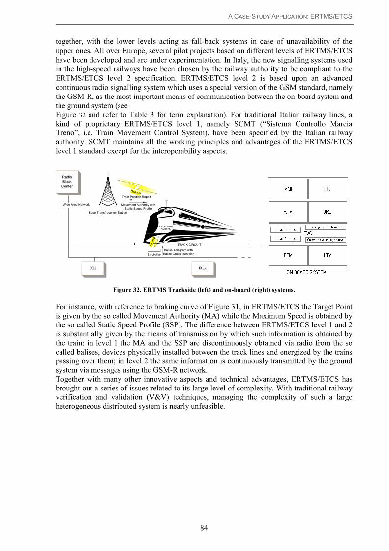
A CASE-STUDY APPLICATION: ERTMS/ETCS
84
together, with the lower levels acting as fall-back systems in case of unavailability of the
upper ones. All over Europe, several pilot projects based on different levels of ERTMS/ETCS
have been developed and are under experimentation. In Italy, the new signalling systems used
in the high-speed railways have been chosen by the railway authority to be compliant to the
ERTMS/ETCS level 2 specification. ERTMS/ETCS level 2 is based upon an advanced
continuous radio signalling system which uses a special version of the GSM standard, namely
the GSM-R, as the most important means of communication between the on-board system and
the ground system (see
Figure 32 and refer to Table 3 for term explanation). For traditional Italian railway lines, a
kind of proprietary ERTMS/ETCS level 1, namely SCMT (“Sistema Controllo Marcia
Treno”, i.e. Train Movement Control System), have been specified by the Italian railway
authority. SCMT maintains all the working principles and advantages of the ERTMS/ETCS
level 1 standard except for the interoperability aspects.
Base Trans/receiver Station
GSM-R
TRACK CIRCUIT
Movement Authority with
Static Speed Profile
Train Position Report
Radio
Block
Center
Wide Area Network
IXLj IXLk
ON-BOARD
SYSTEM
Eurobalise
Air-gap
Balise Telegram with
Balise Group identifier
Figure 32. ERTMS Trackside (left) and on-board (right) systems.
For instance, with reference to braking curve of Figure 31, in ERTMS/ETCS the Target Point
is given by the so called Movement Authority (MA) while the Maximum Speed is obtained by
the so called Static Speed Profile (SSP). The difference between ERTMS/ETCS level 1 and 2
is substantially given by the means of transmission by which such information is obtained by
the train: in level 1 the MA and the SSP are discontinuously obtained via radio from the so
called balises, devices physically installed between the track lines and energized by the trains
passing over them; in level 2 the same information is continuously transmitted by the ground
system via messages using the GSM-R network.
Together with many other innovative aspects and technical advantages, ERTMS/ETCS has
brought out a series of issues related to its large level of complexity. With traditional railway
verification and validation (V&V) techniques, managing the complexity of such a large
heterogeneous distributed system is nearly unfeasible.

A CASE-STUDY APPLICATION: ERTMS/ETCS
85
Term Meaning Brief Explanation
ASF Ansaldo Segnalamento Ferroviario The Italian branch of ANSALDO SIGNAL, a leading company in the
railway signalling industry.
ATPS Automatic Train Protection System Used to protect train movement against the allowed speed profiles.
BG Balise Group A set of identical balises grouped together to allow data redundancy and to detect train direction.
BTM Balise Transmission Module Device used by the on-board system to read data from balises.
BTS Base Transmitter-receiver Station Used for GSM-R communication and distributed along the track.
ERTMS/ETCS European Railway Traffic Management System / European Train Control System
The new European standard for railway signalling and train control systems.
Eurobalise (or
simply Balise)
- Device installed between rail lines used to transmit static (e.g. position)
and/or dynamic (e.g. MA) data to the on-board system.
EVC European Vital Computer The on-board embedded computing sub-system.
GSM-R Global System for radio communications - Railways
A reliable GSM standard specifically developed for railway signalling.
IXL Interlocking System Used to provide train routing, to detect track circuit occupancy status and
other emergency conditions, and to provide the traditional signalling (by light signals) still mandatory in ERTMS/ETCS level 1 (and in SCMT).
JRU Juridical Recording Unit Device used to record train events for diagnostic and legal purposes.
LTM Loop Transmission Module Device used by the on-board system to read data from track circuits (or
“loops”).
MA Movement Authority The distance a train is allowed to cover in safe conditions, used by the on-board system together with SSP to build up the braking curve.
MMI Man Machine Interface Used to allow train driver interact with the on-board system
PR Train Position Report Used in ERTMS/ETCS level 2 by the train to send to the RBC its position
(obtained from the last read balise) together with other data (e.g. speed, operating mode, etc.).
RBC Radio Block Center Used to provide train distancing by communicating with the on-board
system via the GSM-R network and with IXL via the WAN.
RTM Radio Transmission Module Device used by the on-board system to communicate by GSM-R.
SCMT Sistema Controllo Marcia Treno An Italian implementation of ERTMS/ETCS level 1, not fully compliant to
the standard.
SRS System Requirements Specification Documents containing the set of requirements that the system must respect.
SSP Static Speed Profile Static speed restrictions due to the physical structure of the track.
TC Track Circuit Used to detect train presence on a specific section of the railway (typically
1350 meters long) and also to transmit information to the train in
ERTMS/ETCS level 1 (and in SCMT).
TIU Train Interface Unit Device used to allow the on-board system’s interaction with train-borne apparels.
WAN Wide Area Network The long distance network infrastructure used to connect the different
ground apparels (e.g. IXL and RBC).
Table 3. Brief explanation of technical terms and acronyms used in this chapter.
1.3. ERTMS/ETCS Reference Architecture
ERTMS/ETCS provides the specification of an On-board, a Lineside and a Trackside system.
The most widespread ERTMS/ETCS Level 2 is based on a fixed-block and continuous radio-
signalling system. The Lineside system is distributed along the track and it is constituted by a
set of Balise Groups (BG), each one made up by one or more (redundant) balises. A balise is a
device installed between rail-lines, which has the aim to transmit data telegrams, containing
geographical positioning information, to the trains passing over it. The On-board system is
installed on the train and has the aim of controlling train movement against a permitted speed
profile (also known as braking or protection curve), which is elaborated on the base of the
information received from the Trackside via the GSM-R radio network. The On-board also
communicates its position, detected by reading balise telegrams, and other data (e.g. operating
mode) to the Trackside via specific GSM-R messages, namely Position Reports. Therefore, in
order to perform train protection, the On-board must be equipped with the following devices:
- RTM (Radio Transmission Module), used to provide a bidirectional communication
interface with the Trackside using a GSM-R Mobile Terminal;
- BTM (Balise Transmission Module), used to energize balises and read their telegrams;
- TIU (Train Interface Unit), used to interface with train borne apparels (traction
control, service and emergency brakes);

A CASE-STUDY APPLICATION: ERTMS/ETCS
86
- DMI (Driver Machine Interface), needed to provide on-board interaction with train
driver for manual procedures, selections, acknowledgements, etc.;
- EVC (European Vital Computer), elaborating the on-board control logic.
The EVC is an embedded, real-time and safety-critical computing system, so we will suppose
it is based on the well-known and highly adopted Triple Modular Redundant (TMR)
architecture (2 out of 3 voting on processor outputs). In order to control train movement, the
EVC has to interface with the on-board Odometer, measuring train speed and distance since
last balise (a balise provides the train with its exact position, thus recalibrating the Odometer).
The Trackside is constituted by the so called Radio Block Centres (RBCs), which have the
responsibility of providing trains with Movement Authorities, Static Speed Profiles and
possible emergency information. In order to detect track status, the RBC needs to collect data
coming from the national Interlocking (IXL) system, which is not object of standardization
and thus of analysis in this paper. Therefore, the RBC needs a safety-critical elaboration
subsystem (let us suppose a TMR system, like the one of the EVC), and two main
communication interfaces:
- GSM-R, in order to communicate with trains in its (limited) supervised area;
- WAN (Wide Area Network), used to interface with IXL, which is distributed along the
track, and with adjacent RBCs, in order to manage the so called train Hand-Over procedure,
activated when a train is going to exit/enter the RBC supervised area.
A scheme of overall system architecture and main data flows is depicted in Figure 33.
BTS GSM-RRBC
WAN
EVCRTM BTM
TIU
DMI
Mobile
Terminal
DRIVER
TRAIN
Balise
Group
Movement Authorities &
Static Speed Profiles
Balise
TelegramLegend
- RBC: Radio Block Center
- WAN: Wide Area Network
- IXL: Interlocking
- BTS: Base Transceiver Station
- DMI: Driver Machine Interface
- EVC: European Vital Computer
- RTM: Radio Transmission Module
- TIU: Train Interface Unit
- BTM: Balise Transmission Module
Position Reports
Trackside
Man Machine Interface
Balise
IXL
Adjacent
RBCs
Track Circuits
Track
conditions
Hand-Over
relations
Figure 33. Architectural scheme and data flows of ERTMS/ETCS Level 2.
The trackside subsystem is the “ground” (or “fixed”) part of the overall signalling system, that
is the entire ERTMS/ETCS system minus the on-board sub-system. The ERTMS L2 trackside
subsystem is mainly constituted by two sub-systems: the route management system (known as
Interlocking, or IXL), which is responsible of train routing and of collecting track circuit
occupation status, and the separation subsystem, made up by the Radio Block Center (RBC)
and Eurobalises, which is mainly responsible of detecting train position and delivering the
correct Movement Authorities (MA) and Static Speed Profiles (SSP) to the trains. The IXL
part has not been standardized in the ERTMS/ETCS specification, so it was possible to simply

A CASE-STUDY APPLICATION: ERTMS/ETCS
87
adapt the already existing national interlocking system. The Italian national IXL is a
distributed system, made up by a series of distributed IXL modules (hence indicated with
IXL1, IXL2, and so on) connected to each RBC in order to detect and transmit route and track
status to the separation sub-system.
The lineside sub-system is made-up by Eurobalises, which transmit a position telegram when
energized by a train passing over them. Such a telegram contains a Balise Group (BG)
identifier that will be included in the train Position Report (PR), together with other
information (e.g. train speed and position detected by the on-board odometer), and transmitted
to the RBC. RBC will use the balise identifier included in the PR and the offset position
measured by train odometer in order to calculate the Movement Authority to be sent to the
train. In fact, RBC has an internal data-base (configured off-line), in which BGs are
associated with their actual position and with Static Speed Profiles (SSP). This information,
together with the track circuit status received from the interlocking system is (nearly) all the
RBC needs to continuously provide trains with their MAs and thus to achieve its separation
functionality. In ERTMS L2 the on-board and trackside communicate by the GSM-R radio
network, especially designed for railway applications, using the Euroradio protocol [10]. Data
is encapsulated in radio messages whose type and structure is standardised in the
ERTMS/ETCS specification.
1.4. RAMS Requirements
ERTMS/ETCS RAMS requirements define the (non functional) dependability related indices
which a system implementation must satisfy in order to be fully compliant to the standard.
The study of the Safety part is not in the scope of this work, so we will consider only RAM
specification. Of course, RAM aspects do not impact on interoperability and safety, therefore
in practice each railway authority is free to relax or strengthen such requirements according to
its own needs. Another assumption for our analysis is that we will not take into consideration
performability indices (e.g. train delays, transmission errors’ contribution, etc.), related to
specific hardware performance and software implementation; we will only consider structural
(i.e. hardware) reliability aspects.
ERTMS/ETCS define three main types of system failure modes:
- Immobilizing Failures (IF), which happen when two or more trains are no more under
full system supervision;
- Sevice Failures (SF), as above but for only one train;
- Minor Failure (MF), another kind of degradation which is not IF or SF.
For each of these failure modes, RAM specification define the required reliability indices (e.g.
MTBF, Mean Time Between Failures) and the contribution coming from different system
parts or abstraction levels (e.g. software vs hardware, Trackside vs On-board, etc.). The
interesting part is that besides system level indices, also constituent level indices are given,
leaving to designers freedom of choice between a system level evaluation, harder in the
modelling phase, and a more conservative constituent based approach, using more reliable
and thus expensive components. The challenge consists in demonstrating compliance to
system level RAM requirements using less reliable constituents. Another useful analysis is
aimed at ensuring coherence and reachability of reliability indices stated in RAM
specification.
Table 4 summarizes the most important indices that will be considered in the following of this
paper (a bracketed asterisk in description indicates a constituent level requirement).

A CASE-STUDY APPLICATION: ERTMS/ETCS
88
PARAMETER DESCRIPTION REQUIREMENT
MTBF-IONB MTBF w.r.t. IFs due to the On-board subsystem > 2.7*106 h
MTBF-SONB MTBF w.r.t. SFs due to the On-board subsystem > 3*105 h
MTBF-ITRK MTBF w.r.t. IFs due to the Trackside subsystem > 3.5*108 h
MTBF-ILNS MTBF w.r.t. IFs due to the Lineside subsystem > 1.2*105 h
URBC RBC Unavailability (*) < 10-6
UBAL Balise Unavailability (*) < 10-7
AIF-HW Overall System Availability w.r.t. hardware Immobilising Failures > 0.9999854
ASF-HW Overall System Availability w.r.t. hardware Service Failures > 0.99987
Table 4. ERTMS/ETCS RAM requirements of interest.
2. Functional analyses for the safety assurance of ERTMS/ETCS
Safety assurance of ERTMS/ETCS required a number of thorough functional analyses
techniques. The methodologies presented in Chapter II have been applied to a real system
implementation, largely demonstrating their effectiveness and efficiency.
This section is based on some of the case-study results published in [64], [66], [55] and [28].
2.1. Functional testing of the on-board system of ERTMS/ETCS
This section describes the application of the functional testing methodology presented in
Chapter II to SCMT, which is the Italian implementation ERTMS/ETCS Level 1.
2.1.1 Architectural model
SCMT is the name of the Italian ATPS to be used on traditional rail lines. SCMT is made up
by two principal sub-systems: an on-board part, physically installed in train cockpit, and a
ground part, distributed near the rail-lines. Two different types of devices are used in the
ground sub-system to interact with the on-board sub-system. The first type of ground apparels
consists in the track-circuits, which are devices using rail-lines to transmit data to the on-
board sub-system, allowing a semi-continuous signalling system. Track-circuits are meant to
send to the on-board system the status of the signals which the train is going to reach. Such
information is constant during the time the train takes to travel along the loop made up by the
rail-lines (typically, 1350 meters long). The second type of device is named balise, which is a
transmitting antenna energized by trains passing over it, constituting a discontinuous
communication system. Balises can be static or dynamic and they are able to provide the on-
board system with more data respect to track-circuits. To be able to update their data,
according to track status, dynamic balises must be connected to a proper encoder system. To
get the information it needs from the ground sub-system, the on-board sub-system has to be
connected to the TCTM (Track Circuit Transmission Module)16
, which receives data
transmitted by track-circuits17
, and BTM (Balise Transmission Module), which energizes
balises and reads their messages. Finally, a Man Machine Interface (MMI) is used to allow
train driver interaction with the on-board sub-system. All these information are managed by
the on-board sub-system which has to ensure train safety by elaborating the allowed speed
profiles (i.e. dynamic protection curves) and activating service or emergency brakes in case of
dangerous situations. The described architecture is depicted in Figure 34.
16 The equivalent of the Loop Transmission Module (LTM) standardized in ERTMS/ETCS Level 1 specification.
17 Data transmitted by track-circuits is often referred to as “codes”.

A CASE-STUDY APPLICATION: ERTMS/ETCS
89
Figure 34. SCMT architecture diagram.
The whole SCMT system had to be tested in order to be validated against safety related
requirements in both nominal and degraded operating conditions. In particular, to reduce
testing complexity, it has been chosen to test separately the ground sub-system by verifying
the correctness of both installation and data transmitted by balises. Therefore, SCMT system
functional testing only regarded the on-board sub-system. However, as aforementioned, the
main issue was that we could not completely rely on system requirements specification as it
often did not extensively cover degraded conditions which constituted critical scenarios for
system safety.
In the following, we will refer to the on-board sub-system as “SCMT on-board”. In order to
accurately select target system’s input-output ports, we represent them through a context
diagram (see Figure 35) and a class diagram, describing structural relationships involved in
system architecture (see Figure 36).
Testing the on-board system for an exhaustive set of input sequences would be unfeasible for
the exponential growth of test-cases. Such a problem, known in the literature as “test-case
explosion”, depends on the number of input variables and on the set of possible values for
each variable. Next section will show how to contain test-case explosion applying proper
reduction rules.
Figure 35. Context diagram for the SCMT on-board subsystem.
DRIVER
Train data, manual commands, key
pressures
Leds, icons, alarms, text
messages
Brakes
activation
Odometry,
train status
Train speed and position
Track-circuits codes, balise
telegrams
TRAIN
SCMT
on-board
GROUND

A CASE-STUDY APPLICATION: ERTMS/ETCS
90
Figure 36. Class diagram for SCMT on-board.
2.1.2 Testing issues
In the systematic testing performed using a black-box approach, the system is stimulated and
verified at the global input/output gates. Referring to the above context-diagram, the black-
box testing scheme of the SCMT system is depicted in Figure 37.
Figure 37. SCMT black-box testing.
In “pure black-box” approach we would rapidly achieve a huge number of test-cases as the
system should be tested for each combination of values of the input variables, thus making
exhaustive testing unfeasible, in reasonable times, for any complex system. For instance, if we
had 10 input variables and each of them could assume 10 different values, the number of
possible input combinations would be 1010
.
2.1.3 Application of the testing approach
In this section we describe the application to SCMT of the functional testing approach
presented in Chapter II. In particular, a software architecture model was used to perform a
preliminary functional decomposition. Logic modules have been separated whenever they
could be proven to be independent and to interact with each other in a well defined way. Such
decomposition was validated by analyzing structural dependencies within software modules.
Function call-graphs based techniques have been adopted, together with traditional structural
tests, to validate system decomposition. After this step, each module (or macro-function) had
to be fed with extensive input sequences in order to check its output behavior. Outputs had to
be accessed by acting on system hardware by means of proper diagnostic instruments
(hardware and software tools). It was important to ensure that such instruments were the less
intrusive as possible, in order not to influence in any way system behavior. This was achieved
equipping the system under test with built-in hardware diagnostic sub-systems and standard
output communication facilities, in order to interface with software diagnostics.
SCMT
on-board OUTPUT INPUT
DRIVER
TRAIN
GROUND
DRIVER
TRAIN
GROUND

A CASE-STUDY APPLICATION: ERTMS/ETCS
91
Figure 38. SCMT system logic decomposition.
As represented in Figure 38, the decomposition of the system into macro-functions (i.e. logic
blocks) to be separately tested followed two directions:
• Horizontal decomposition, which was based on input-output relations;
• Vertical decomposition, by superposition of progressive complexity levels.
The horizontal decomposition highlighted the well defined data path from inputs to outputs,
i.e. a generic block is influenced only by external inputs and output of the previous block, but
not by the other surrounding blocks. Vertical decomposition consisted in considering the
system as the superposition of different working levels, from the simplest to the most
complex, in a bottom-up way. The upper levels introduced new functionalities relying on a
new set of external influence variables. In such a way, the system was divided in distinct logic
blocks, for instance Braking Curve Elaboration (horizontal level) for Complete SCMT
(vertical level).
Each logic block was influenced by a well defined set of inputs and reacted with outputs that
could be either accessible or not at the system’s output interfaces. In case the output was not
visible, internal probes had to be used to access the part of the system state we were interested
in.
A test-case classification according to the introduced logic blocks was possible, with each
block was associated with its own test suite. In particular, the first level horizontal
decomposition of SCMT was constituted by the following blocks (see Figure 39):
1. SCMT System Logic, which had the aim to apply the correct “work plane”;
2. Braking Model Elaboration, aimed at building the proper protection curves;
3. Braking Model Application, which had to control the braking distance.
The same decomposition is very likely to apply to all classes of brake-by-wire system, in
which the first block (on the left) collects and elaborates external data (coming from input
devices), the central block computes the output of the reference braking model, while the last
block (on the right) controls the correct respect of the braking profile (as detected by on-board
odometer). A slightly modified scheme should apply to fly-by-wire system, respecting the
general division between data collection and elaboration, reference flying-model computation,
respect of the model profile or flying route (comparing expected position with the one
collected by airborne sensors, e.g. altimeter, GPS, radar, etc.).
Internal variables had to be assigned values, for testing purposes, acting on the corresponding
external input variables. In order to perform this operation, we needed to know the functional
behavior of the previous block (obtainable by the specification) and to test it previously to
ensure its correct implementation. For instance, having already tested the first horizontal
block, it was straightforward to obtain the corresponding external inputs by means of a
TARGET SYSTEM
Vertical Decomposition
Horizontal Decomposition
Vertical Level I
Vertical Level III
Vertical Level II
H. Level III H. Level II H. Level I
SCMT
Complete SCMT
Partial SCMT
Basic SCMT
System
Logic
B. Curve
Application
B. Curve
Elaboration
S.L.
1 …
S.L.
3 2nd Stage of Horizontal Decomposition
1st Stage of Horizontal Decomposition

A CASE-STUDY APPLICATION: ERTMS/ETCS
92
backward analysis from “internal” outputs (i.e. D0, V0, etc.) to external inputs (i.e. the real
influence variables). This process could be iterated for every block.
Figure 39. First-level horizontal decomposition of SCMT in detail.
SCMT vertical working levels are related to the completeness of the information received
from the ground sub-system. At the Basic SCMT level, on-board sub-system only reads codes
from track-circuits. At the Partial SCMT level, only information from static balises are added
to the codes. Finally, in Complete SCMT level all ground transmission devices are used to
collect data. It is important to underline that while real SCMT working levels contain
incremental functionalities (e.g Partial SCMT comprises Basic SCMT), vertical levels shown
in Figure 39 feature differential functionalities (e.g. Partial SCMT contains all the functions
not already contained in the lower level). Such a distinction allowed us to reduce test
redundancies, by verifying only the new functionalities at each working level, in a bottom-up
way.
Finally, we were able to divide the target system into 15 blocks, with an influence variable
average reduction factor of 2 for each block (further augmentable with other techniques). To
estimate the achieved reduction factor, we considered Equation 1. For SCMT we achieved an
overall reduction factor, at this stage, of more than 100.
SCMT influence variables could be divided into the following two main groups:
• Scenario variables, which represented operating conditions (e.g. track circuit length
and transmitted codes or code sequences, balises messages, etc);
• Test-Case variables, which represented specific inputs for a given scenario (e.g. train
speed, key pressures, etc.).
At a first step, we identified all the possible influence-variables. Then, in order to reduce the
number of influence variables for each logic block, we developed a simple procedure of
variable-selection, with a step-by-step independence checking: if the value of a certain
variable was directly deductible from the others, then it was excluded from the set of
influence variables because it would have led to define further test-cases which, however,
would have revealed equivalent to at least one of the already developed. For instance, for the
proper working of the “SCMT System Logic” blocks, it was necessary to define a set of
variables needed to express at least the following information: the completeness of the ground
equipment (only track-circuits, track-circuits and static balises or track-circuits and dynamic
balises), the type of installed balises and the consistency of the information contained in
balises. On the basis of the requirements contained in system specification, we found out that
the variable expressing that data consistency of balises was always dependant on the first two
variables. Thus, such a variable was excluded from the set of influence variables, being
redundant. Another simple example of a redundant variable consists in the one expressing the
“Train Stopped” condition. Such a variable was always used in combination with “Train
Speed”, and its value was dependant on “Train Speed” value, because the train was
considered stopped if and only if train speed was less than 2 Km/h.
Output variables classification was performed starting from the logic block(s) they influenced.
In particular, to access “hidden outputs”, that is outputs that were not normally accessible
from the interacting entities, we need to know system physical structure. For instance, let us
refer to the first level horizontal decomposition shown in Figure 39. In such case, the
stimulating variables were Do, Vo, VT, while the output variables to be probed were Sn, Sa, Sc.
Sn,Sa,Sc Do,Vo,VT
Braking Model Elaboration SCMT
System
Logic
Braking
Model
Application

A CASE-STUDY APPLICATION: ERTMS/ETCS
93
The former variables were assigned values by properly acting on external accessible inputs,
while the latter could be read from the log-files generated by the diagnostic software
managing hardware probes.
A tree-based test-case generation technique was applied to every logic block. At each level,
only one influence variable, among the ones not already instantiated, was assigned all the
significant values of its variation range, according to the reduction criteria that will be
described later in this section. Influence variable instantiation could be divided into two
macro-levels: scenario variables and test-case variables. In fact, test-cases were introduced
only when all the significant operating scenarios had been defined. The combination of the
instances of the variables was performed automatically by a tool meant to apply a set of pre-
determined reduction rules (described later on in this section), for an “a priori” pruning of
pleonastic tree branches. With such an approach, tree leaves represented the test-cases which
had to be actually executed.
The main reduction criteria adopted have been:
• Incompatible combination of scenario or test-case variables;
• Not realistic operating conditions (for scenario variables);
• Equivalence class based reduction (considering scenario parameters or input variation
ranges);
• Context specific reductions (i.e. context-specific dependencies, code-based static
independence checking, mapping on test-cases already defined for a different logic block,
etc.).
For scenario variables, the conditions to assess “incompatibility” were usually based on
constraints coming from the physical environment, while “realistic operating conditions” refer
to the railway national or international norms prescribing a set of requirements that must be
necessarily respected [114]. Some of these norms are about track circuit length, balise
positioning, signalling rules, etc.
For test-case variables, context specific dependencies were very frequent and could be found
when the assignment of some particular values or ranges of values to a specific set of
variables implied a fixed value assignment for another distinct set of variables. Also code-
based independence checking was used in order to avoid repetition of simple tests (e.g. key
pressure failures) in different SCMT operating modes, when it could be proven that the called
managing procedure was the same. Finally, as test-cases stimulated different logic-blocks,
often only one execution was performed for multiple defined tests (what increased was the
output checking time for the same test).
The most complex and efficient technique was based, both for scenario and test-case
variables, on equivalence class based reductions. An equivalence class represents a set of
valid or invalid states for a condition on input variables. The domain of input data is
partitioned in equivalence classes such that if the output is correct for a test-case
corresponding to an input class, then it can be reasonably deducted that it is correct for any
test-case of that class. By tree-generating the combinations of influence variables and
reducing them with an equivalence class based approach, it was implemented what is called
an extended SECT coverage criterion. SECT is the acronym of “Strong Equivalence Class
Testing”, which represents the verification of system behavior against all kinds of class
interactions (it can be extended with robustness checking by also considering non valid input
classes). In our case, SECT was feasible because each logic block had a quite small number of
influential variables, each one assuming a small number of classes of values.
Generally speaking, when we had to select input values for influence variables we chose at
least one test-case for each of the following classes: internal values, high-boundary values,
low-boundary values, near high-boundary values, near low-boundary values, over high-
boundary values, below low-boundary values, special values (only for discrete variables). The
last three classes were very important to test robustness (and thus to ensure system-level
safety). Therefore, a non Boolean variable assumed at least three different values, belonging

A CASE-STUDY APPLICATION: ERTMS/ETCS
94
to the first three categories. The followed approach included “Boundary Analysis”,
“Robustness Testing” and “Worst Case Testing” (WCT) techniques18
. In some cases,
according to system specifications, we merged the three techniques by adopting nearness,
robustness and worst-case conditions. For instance, train speed ranges have been first
partitioned into sub-sets, according to the specified speed limits, that is: V<2 Km/h,
2Km/h<V<15Km/h, 15Km/h<V<30Km/h, etc. The obtained sub-sets represented all the
significant train speed ranges used in the entire system specification. However, for all tests in
which we were testing a function which only required the train to be under a maximum speed
limit (VMAX), train speed values were chosen as follows: V=1/2 VMAX; V=VMAX - δV;
V=VMAX + δV (where δV is a small positive speed value, for instance 1Km/h). The so defined
speed values were combined with all the remaining influence variable values, even in the
worst-case conditions.
The next stage consisted in determining expected outputs for each test-case. Examples of
measured output variables are: leds (on/off), icons, text messages, brake intervention, train
position, etc. System behavior was modelled in terms of significantly varying outputs and
their expected values. The correct behavior was directly obtainable from system
specifications, but, in some cases, it had to be derived by means of a parallel independent
model. Comparison of the results was then made manually. For instance, we used a parallel
independent model for the braking curve prediction based on a human comparator. When the
described approach was able to highlight incompleteness or incoherence in system
specifications, it was necessary that the responsible for system specifications assessed the
correct system behavior corresponding to the identified input conditions. Finally, as an
operational tool, we made use of a spreadsheet in order to represent Test Case Specification in
terms of: operating scenario, represented by instantiated scenario variables (e.g. TC code
sequence: CODE1→CODE2); input sequences, represented by test-case variable values and
their associated time-line (e.g. key X pressed within time T); expected outputs and optional
measurement instructions (e.g. icon Y appearing on the MMI display and recorded as variable
Vy in log-file L).
Fig. 1. Example of using a parallel model in SCMT.
A relevant amount of tests had to be executed on the SCMT system, so it was useful to
identify priority levels for test classes. The main criterion was the safety criticality of
functions/blocks, identified by the hazard-analysis processes [121], used to validate system
specification against the most critical causes of dangerous failures. For instance, correctness
of system behavior was first tested against the so called “restrictive input sequences”, that is
track-circuit code sequences that should activate one or more train protection mechanisms.
Moreover, in testing the system for any new software version, we adopted a “width-first”
coverage strategy, that consisted in executing the most significant test-cases for each block
18 Such techniques are based on empirical studies. For instance, it has been noted that most errors generate in
correspondence of extreme values of input variables.
COMPARATOR
Sn,Sa,Sc D0,V0,VT
Protection curve elaboration SCMT
System
Logic
Braking
model
application
PARALLEL
INDEPENDENT MODEL
for curve elaboration
=

A CASE-STUDY APPLICATION: ERTMS/ETCS
95
and category, in order to quickly discover and notify macroscopic non conformities or
dangerous behaviors.
Test-cases have been executed in a simulation environment made up by: the system prototype
under test; hardware devices simulating external interactions (i.e. system inputs); software
tools aimed at simulating the operating environment (i.e. the scenario) and allowing the
automation of the test process through batch-files. To speed up test process, preparation,
execution and output verification activities have been pipelined, in order to allow more test-
engineers work in parallel. Comparison of the output log-files with the expected outputs had
to proceed manually in the first phase of test execution, because Pass/Fail criteria were often
based on time/speed ranges, very difficult to validate in a complete automatic environment. In
all cases a faulty behavior has been observed, a proper notification (i.e. System Problem
Report) was sent to the development division. Such a notification could regard, as
aforementioned, implementation errors as well as specification errors. The testing
environment used for SCMT has been depicted in Figure 40.
In order to verify the correct implementation of needed modifications and to ensure the
absence of regression errors, the whole set of tests had to be repeated at any new software
version. This is the most simple and safe non-regression testing technique, known in literature
as “Retest-All” [143], which was easily applicable due to test automation. The automation of
the check for correctness of output log-files was performed using a Gold-Run technique [15].
Figure 40. Test execution pipeline.
The approach described in this section allowed test engineers to define and execute more than
2500 test-cases, covering all the functionalities of the system in normal as well as in degraded
states of operation. The revealed errors contributed to improve system specifications in terms
of both correctness and completeness. The application of the innovative testing approach
allowed to improve test coverage while reducing the number of required test-cases. An
extensive documentation activity (test plan, test design specification, test case specification,
etc.) helped improve organization with the result of speeding up test execution and facilitating
test reproducibility. The verification of coverage by code instrumentation showed a coverage
(using a Decision to Decision Path technique [13]) of nearly 90%, which did highlight the
effectiveness of the testing approach. The uncovered parts of software were verified apart,
resulting almost exclusively in defensive control branches. In past experiences, such a high
level of coverage was only obtained by means of dynamic white-box tests in simulated
environments, which however did not give test-engineers the same level of confidence of
system tests in assuring system correct operation, for the following reasons:
• task interaction was limited to the phases of interest;
• hardware-software integration was not tested, as commercial PCs were used instead of
target hardware;
• the simulation environments are not validated, as this is usually considered not worth
the significant effort required.

A CASE-STUDY APPLICATION: ERTMS/ETCS
96
2.2. Model-based reverse engineering for the functional analysis of ERTMS/ETCS control logics
In this section we show how we applied the model-based static analysis technique to the
control software of the Radio Block Center, using the Unified Modeling Language (UML), as
explained in Chapter II §3.
Figure 41. RBC software architecture.
2.2.4 RBC control software
The software architecture of the RBC is depicted in Figure 41. There are some “application”
processes (written in a safe subset of the C programming language), which manage the
interaction of the RBC with the external entities (i.e. other subsystems and the RBC operator),
and some “logic” processes, which instead implement the control logic of the RBC; the latter
are written in an application specific logic language, as already mentioned above.
The logic manager has to interpret logic language, translating it into executable code, and to
schedule the logic processes, while the shaded rectangles in Figure 2 represent the logic
processes, which are the target of our work. For instance, the “MA” process, shown in Figure
2, verifies the integrity of the Movement Authority assigned to the train against all the
significant track and route conditions. Such conditions are received from the interlocking
system by means of the “IXL interaction” application process and are managed by the “TC”
logic process, which stores Track Circuit physical conditions in its internal variables. If the
MA integrity verification fails (for instance a track circuit is not clear or involved in an
emergency condition), the MA process has to command the sending of an emergency message
to the “Train interaction” application process, which will manage the sending of the proper
radio messages to the train. In this simple example, the MA and TC processes interact with
the application processes to manage data from and to the external subsystems; moreover, they
interact with each other, as the MA process asks the TC process for the status of track circuits,
in order to verify the integrity of the movement authorities.
There are many other logic processes which behave in a similar way. They can feature:
- a set of data variables and a special “process status” variable;
- a set of “operations” which can be activated: by application processes or the RBC operator
by means of “manual commands”; by other logic processes, issuing “automatic commands”;
directly, when the process status variable is assigned a certain value.
Typical process operations are:
- verify conditions on internal variables or on the ones of different processes;
- assign values to internal or other processes’ variables (the logic manager does not restrict the
visibility and modifiability of variables);

A CASE-STUDY APPLICATION: ERTMS/ETCS
97
- issue automatic commands to other processes; issue “application commands” to application
processes (e.g. “send MA”).
2.2.5 Reverse engineering and static verification of the RBC
In this section, the modeling technique from RBC logic language to UML diagrams is
described referring to the very simple “Change of Traction Power” (CTP) logic process. The
CTP process has to manage manual commands of activation/deactivation of a change of
traction power line section, coming from the RBC operator. The activation/deactivation
command must be accepted only if the track circuit in which there is a change of power is free
and not included in a MA assigned to a train. In the following we present the modeling rules
in the building of UML views for such example process.
Figure 42. Use case (left) and class (right) diagrams for the CTP logic process.
- Use case diagrams (see Figure 42, left): they represent how a logic process can be used by
application processes or the operator using manual commands; therefore, they represent the
externally triggered high-level procedures.
- Class diagrams (Figure 42, right): they are built from a static software architecture view
(data structure with internal/public attributes, operations), also showing the relationships and
interactions between processes (variable read/write, procedure call). They represent the
backbone of the entire model, as the first modeling step consists is the definition of a class for
each of the logic processes. The relationships between classes are determined by the “access”
or “assign” statements (as aforementioned, all process variables are seen as public) and by the
issuing of commands, triggering process operations. Given the high number of associations
(some processes can share up to 20 distinct links) a comprehensive class diagram would be
very complex and almost unreadable. We preferred to build up partial class diagrams, each
one focusing on a single process and showing all the incoming and outgoing links to/from that
process. The CTP process features three local variables, a single “outlinked” process and two
operations. In case a process only accesses (or “reads”) data of another process (usually to
check some conditions on the state of the other process), the link is modeled by a dependency
relation (dashed line). In case, instead, the process also activates operations of the other
process (by automatic commands), the link is modeled as a real association (full line). If the
modeler does not need to build an executable model (as in our case), he/she does not need to
be fully compliant to the UML standard, and can therefore adapt the notation to his/her needs.
For instance, we also associated to relations a list of accessed variables and operation, as a
further documentation. From the class diagram, we see that CTP process is used by the MA
process: in fact, the MA process has to manage the presence of a CTP section as an additional
information to be added to the outgoing MA message in order to inform the on-board system
of the CTP procedure. From the CTP class diagram it is evident that a first refactoring is
necessary: class attributes must be kept private, and a Get_CTP_State() must be added in order
to get CTP state.

A CASE-STUDY APPLICATION: ERTMS/ETCS
98
Figure 43. Sequence (left) and state (right) diagrams for the CTP logic process.
- Sequence diagrams (Figure 43, left): they are specified for each operation, showing its
implementation and detailed interactions between logic processes. A full arrow has been used
for check and assignment statements, specifying the nature of the operation as a comment. A
normal arrow is used, instead, for the activation of an operation. For better clarity, each
complex diagram has been detailed using linked notes. In Figure 43 we report an example
sequence diagram for the CTP process, showing the activation operation (the deactivation is
very similar): when an activation command is received, the state of the associated TC
(belonging to a properly declared linked processes list) must be checked in order to verify if it
is in the “free” and “not requested” (for a MA) states. If the condition is satisfied, the
automatic command Set_CTP_Active() is issued to the TC process.
In general, the traceability and verification of compliance was performed as follows. Using
sequence diagrams, the execution process was statically analyzed from the external activation
of an operation (by a “manual command”) to the reaching of a stable process state, e.g. the
one following the sending of a message to an application process. A proper package named
“Scenarios” containing all scenario sequence diagrams was created for the traceability
analysis. Each “composed” or “high-level” sequence diagram represents a scenario of e.g.
Start of Mission, Hand-Over, Emergency, and so on. For instance, we discovered that in some
cases the controls on the actuability of a manual command were missing. In particular, an
emergency message to a non existing train number caused the RBC to crash. Usually, such
errors are revealed in the functional testing phase, while the approach described in this paper
allowed us to detect them earlier in system validation process. Furthermore, by tracing
sequence diagrams into functional requirements, we discovered some pieces of code related to
never referenced operations, which were inherited from an early specification: an application
of refactoring, in this case, consisted in removing such pleonastic operations and attributes.
- Statecharts (Figure 43, right): they show the transitions of the state variables of the logic
processes against the triggering events. The CTP statechart has been simplified to be self
explaining. Clearly, for the CTP process all input conditions at any state have been
considered, and there are no unreachable or deadlock states (which have been detected and
corrected for some other processes).
Finally, let us present a refactoring example which is quite general. From the analysis of
sequence diagrams, we realized that most of the RBC logic code was made up by condition
verification statements. Therefore, by properly grouping and shifting conditions we were able
to predict and minimize the number of controls performed at each elaboration cycle, thus
improving system performance and directly impacting on the number of trains the RBC was
able to manage (final gain was about the 30%). For instance, if a TC is interested by an
emergency, there is no need to check its occupation status: immediately after the emergency is
detected, an emergency message must be sent to the train. Thus, it would be natural to choose
such control as the first to be performed. However, the probability of an emergency is very
low, and such a check would be false most of the times, wasting elaboration time, so it is
better to put it in the end of the control chain.

A CASE-STUDY APPLICATION: ERTMS/ETCS
99
With respect to previous projects of similar complexity, the RBC static verification process
was speeded-up by several times and the number of revealed bugs at this stage (before any
dynamic analysis) was more than double (the final number of discovered errors remaining
approximately the same). As a further advantage, the availability of a model also allowed us
to reduce the time to find the cause of errors detected during the following functional testing
phase.
2.3. Functional testing of the trackside system of ERTMS/ETCS
In this section we deal with the functional validation of the trackside part of an ERTMS/ETCS
compliant system. An extensive set of functional tests need to be specified in order to
thoroughly verify the system, using the innovative approach based on influence variables and
state diagrams described in Chapter II. The statechart based reference model allowed for
extensive scenario based test-case specification and reduction.
Such a detailed test specification requires a great amount of time and resources to be entirely
executed in the real environment. Moreover, several tests need to generate abnormal safety-
critical conditions that are unfeasible on the field. In this section we also describe how we
overcame such problems by developing a flexible distributed simulation environment for
anomaly testing and test automation based on a scripting language with both execution and
verification capabilities.
2.3.1 Introduction
The most important aspect in testing the ERTMS/ETCS trackside subsystem was the
verification of interoperability and safety requirements. Compliance to ERTMS/ETCS, in
fact, means also interoperability of trans-European rail lines. Safety, of course, was the most
important aspect: all the functional safety requirements, obtained by the preliminary hazard
analysis process, were to be thoroughly verified. This implied a detailed functional test
specification, based on the concepts of influence variables, firstly introduced in the SCMT
system validation, and state diagrams, found to be the best way to represent the behavioral
aspects of a very complex system, as the one under test. In the total scheme of the assurance
tasks (hazard analysis, static code analysis, etc.), functional testing plays, according to our
experience, the most important role, in terms of required time, budget and visibility (it is one
of the last activities to be performed before system activation).
The main problem was that such a thorough test specification included more than 2000 tests,
many of which were not reproducible in real conditions, as they regarded extensive
combinations of abnormal conditions, negative inputs, degraded states of operations, etc.
Thus, the testing team had to deal with the following three issues:
• a lot of test conditions (about the 30%) were not feasible in the real environment;
• the time to execute the tests in the real environment was excessive (it would have taken
several years);
• the real environment does not allow to automate test execution, and this is a serious
problem when dealing with regression testing (the entire test suite must be repeated at
any new software version).
Therefore, a simulation environment had to be developed and fine tuned to match the needs of
the test engineers, consisting in simulating both nominal and negative test conditions, also in
degraded states of system operation. Finally, the simulation tools had to be able to support
batch execution by means of proper script management capabilities, in order to automate the
test process.
The “system in the loop” [8] simulation environment described in this paper together with a
specifically designed anomaly management tool allowed the testing team to define by script
files and automatically execute most of the specified functional tests in a few months,
detecting several unconformities and implementation errors (test suite execution is still in

A CASE-STUDY APPLICATION: ERTMS/ETCS
100
progress).
A context diagram of the trackside subsystem is reported in Figure 44.
Figure 44. The trackside context diagram.
2.3.2 Application of the test specification methodology
As described in Chapter II, traditional functional testing techniques allow to verify system
implementation against its requirements, but it is beyond their scope to validate system
requirements specification; natural language specification, however, even though revised, is
often incomplete, so a stronger technique is needed. This technique should merge the main
objectives of safety and feasibility. The test specification for the ERTMS/ETCS trackside
system had to guarantee:
• The complete coverage of system functional requirements, both in nominal and degraded
states of operation (“negative testing”);
• An in depth analysis of system scenarios aimed at detecting operating conditions not
covered by system specification (using the concept of “influence variables”, as described
in Chapter II);
• The minimization of the number of required test-cases, to ensure the feasibility of the
functional testing phase;
• A structured and systematic test specification, documentation and execution process,
aimed at an easier data understanding and management, to be shared by a large group of
test engineers.
The result of considering all these needs was a test specification methodology based on
influence variables and represented by state diagrams. The influence variables are all system
variables that are able to influence its behavior and have been divided in input and state
variables. The resulting state diagrams represented all the system operating scenarios that are
ideally linkable all together to represent the overall functional behavior of the system under
test.
The test specification process is made up by the following steps:
• Detection of system boundaries, to highlight input-output gates;
• Elaboration of a list of base operational scenarios, to be used as a starting point for the
functional analysis;
• For each scenario, detection and reduction of influence variables (system level variables,
obtained by the specification, influencing system behavior);
• For each scenario, representation of system behavior in the functional scenario by means
of a state diagram;
• For each state, generation of the elementary test-cases (simple “input-output-next state”
relations);
• Generation of scenario test-cases, by linking elementary test-cases.
OPERATOR
Temporary Speed Restrictions, emergencies
Diagnostic alarms, line and train
status
Radio messages (e.g. MA)
Radio messages
(e.g. PR)
TRAIN
Hand-Over variables (accepting / handing-over)
NEIGHBOUR RBC LINE
ERTMS/ETCS
Trackside
(RBC+IXL)
Track-Circuits and route status, emergencies, out
of service, etc.
Status of the light signals used for
entering/leaving the ERTMS L2
equipped line

A CASE-STUDY APPLICATION: ERTMS/ETCS
101
More specifically, the following were the significant state variables for the trackside system:
• Track status (managed by IXL): track circuit occupation (used to compute the Movement
Authority); route integrity (e.g. “switches out of control”); emergency conditions (e.g.
“line out of service”).
• Train status (as seen from the RBC): information received by means of the train Position
Report (train speed and position, as computed by the odometer, and Last Relevant Balise
Group read by the train); information previously managed by the RBC (Movement
Authority and SSP assigned to the train, list of messages waiting for an
acknowledgement, list of emergency messages transmitted to the train).
• RBC status: list of radio messages sent to the train; list of radio messages received from
the train; route status (i.e. route assigned to the trains); emergency and Temporary Speed
Restrictions input from operator.
Analogously we could define the input from trains (i.e. radio messages), from track (e.g. track
circuit occupation) and from operator (e.g. Temporary Speed Restrictions on the line), which
have to be managed from the trackside in any state.
As for the expected trackside behavior, most of the outputs directly regard RBC, which is the
most complex and important subsystem, because it collects data from the track and directly
interacts with the on-board subsystems. Generally speaking, there are some common aspects
in RBC reaction against a particular input, which we briefly list in the following:
• When it receives an emergency condition from the IXL or from the human operator, it
reacts sending a proper emergency message to one or more trains;
• When it receives a Position Report from a train, it stores the relevant information and
verify the possibility to assign it a new Movement Authority;
• According to the track freedom and route integrity received from the IXL, it chooses the
length and the operating mode (Full Supervision, On-Sight or Staff Responsible) of the
Movement Authority to be sent to the trains;
• When actuating a procedure, that is a sequence of predefined operations, it ignores a set
of “safe” unexpected messages received from a train while it orders a disconnection if the
message is considered “unsafe”;
• During a procedure, it passes from a state to another when it receives an expected
relevant message from a train or a condition from the trackside;
• It manages some sets of messages at any phase of train mission (i.e. during any
procedure), such as disconnection requests and validated train data.
The combination of a system state, a relevant input condition, an expected output and state
transition constitutes an elementary Test Case for the system, while several Test Cases linked
together in order to reproduce a complete evolution of the system under test in a given
scenario is named a Test Scenario, as defined in Chapter II.
Master
Simulator
Simulated IXLs Real IXLs
Route Formation Commands,
T rack Circuit Occupat ion,
Degradat ions
Radio Block CenterSimulated
neighbor RBCs
Simulated On-Boards
Anomaly Manager
Train Driver Commands,
Balise Telegrams,
T rain Speed and Posit ion
Output
Log-File
s
Script Manager
Radio messagesT rack and route status relations
Hand-Over
relations
Figure 45. A logic scheme of the testing environment.

A CASE-STUDY APPLICATION: ERTMS/ETCS
102
2.3.3 The simulation environment
The IXL modules (see Figure 32) are distributed all along the track, at an average inter-
distance of 12 km and are normally remote controlled by a central control room. There are
several types of IXL modules, that we distinguish here only into “line” and “station”
categories for the sake of simplicity. The Radio Block Center, instead, is physically installed
in the central place and communicates with neighbour RBCs and its IXL modules by means
of a high-speed long-distance fiber optic backbone (redundant). Given the complex
architecture of the system under test, it was not easy to create a simulation environment that
was both realistic (all the real hardware and software to be tested had to be used) and flexible
(the external environment had to be completely programmable). A classic “system in the
loop” scheme was adopted for the simulation environment; however, the hard task was to
adapt the tools used to stimulate the system in normal operating conditions, that were already
developed, in order to make them able to be used to generate non nominal (or negative) ones.
The simulation environment is made up by the following elements (see Figure 45):
• a real RBC;
• a pair of simulated RBCs (its neighbours);
• a certain number of real and simulated IXL modules (the ones in its supervised area);
• a certain number of on-board simulators, used as a sort of input injectors and output
probes with respect to the trackside;
• a so called master simulator, used to control and stimulate all the simulated entities.
The choice of real and simulated sub-systems is given by two contrasting factors:
• the realism of the environment, which would suggest the use of all real sub-systems;
• the flexibility of the environment: most negative and degraded conditions are either
impossible or very difficult to obtain with the real systems.
The master simulator is a tool used to command the on-board and IXL, in particular by
stimulating:
• the on-board simulator with train-driver, balise and trainborne (speed, diagnostic)
inputs;
• the IXL with track conditions (track circuit occupation, degradations of route status,
emergencies).
The configuration of the real RBC was based on the same hardware and software used on the
field, comprising a vital section constituted by the following parts:
• a safety kernel with three independent computing subsystem in a Triple Modular
Redundant configuration, which manages the train separation;
• a Man Machine Interface (MMI) constituted by a video terminal (showing train data),
a track display (showing train position and track status) and a functional keyboard
used by the RBC operator to digit commands to be sent to the trains (e.g. temporary
speed restrictions and emergency messages).
The non vital section is made up by the following systems:
• two communication computers, used to communicate with IXL and on-board sub-
systems;
• a redundant chronological event recorder, that is a sort of extended Juridical
Recording Unit (JRU), with the aim of recording the times and nature of the
significant events (e.g. diagnostic data, alarms).

A CASE-STUDY APPLICATION: ERTMS/ETCS
103
The extended JRU is also used to read after-test data in order to compare obtained outputs
with the expected ones (such comparison is partly automated).
All the real and simulated entities were connected in our laboratory by means of a normal
LAN (Ethernet 100Mb/s).
Figure 46. The hardware structure of the trackside simulation environment.
Each of the simulated sub-systems (i.e. each simulated on-board, RBC, or IXL module) was
installed on a different general purpose computer (see Figure 46). The software simulators
were complete, showing all the features of a real MMI on the PC screen. The master simulator
together with the train simulators allow to simulate the trains marching on a certain track
section, showing their speed and positions and simulating track circuit and route occupation.
In order to allow test automation, both in the real systems and in the simulated ones it was
installed some tools which communicate with a central master by which it is possible to
command all the systems and create all the abnormal and degraded conditions which could
happen in a real operating situation. A scripting language was implemented in order to specify
batch sequences, that is to say the commands of the master simulator used to execute the
complete test scenarios.
The last element of the simulation environment is the on-board simulator. It has been
developed to simulate the behavior of a real train and properly adapted in order to generate
anomalies that, otherwise, would be very hard or impossible to obtain with a real train. The
simulation of anomalies with the on-board simulator is the main topic of the next section.
2.3.4 Simulation of anomalies
The communication between the RBC and the on-board and between the RBC and the IXL
uses an open network. The CENELEC 50159-part 2 norms report the threats of a
communication based on an open network (i.e. deletion, re-sequencing, insertion, repetition,
delay, corruption and authentication of a message; see Table 2) and suggests some means to
ensure the safety of the system with respect to such threats. The communication protocol
employed for the data exchange from and to the RBC is CENELEC compliant and should
protect from all the aforementioned threats [121]. The functional analysis used for test
specification had to consider all the possible threats also in degraded operating conditions
(e.g. a degraded route due to a loss of control of one or more switches) in order to exercise the
robustness of the systems and of the communication protocol.
Therefore, the simulation environment has to be able to simulate both degradations and
malfunctions. The “standard” environment is able to create all the degradations of the
signalling system, which are abnormal railway conditions which the system must be able to
properly manage. The simulation of railway degradations is useful to verify that the RBC is

A CASE-STUDY APPLICATION: ERTMS/ETCS
104
able to understand and react correctly to such conditions, ensuring the safety of train
movement.
However, a standard environment is not able to reproduce the anomalies of the
communication between the RBC and the on-board, which can happen in real operating
conditions. In fact, the same threats reported in the CENELEC 50129 part 2 can affect the
communication by the GSM-R network and both the robustness and the protection
mechanisms implemented at different levels (protocol, application, etc.) must be verified in
the functional testing phase.
For the above considerations and due to the need for testing the train separation system in all
conditions with all combinations of its significant inputs, the simulation environment had to
be adapted and customized in order to simulate in laboratory all the aforementioned
communication anomalies.
The first step was the analysis of test specifications in order to identify the tests related to
communication anomalies. We found out that only the 13% of the specified tests
corresponded to nominal operating conditions; the remaining 87% were degradation or
anomaly tests (respectively the 52% and the 35%). On the basis of such analysis and
classification, we implemented a so called “anomaly manager” tool, which was completely
independent from the nominal simulator.
The abnormal conditions that have been detected and implemented are the following:
• deletion of any message from a train to the RBC;
• deletion of any message sequence (i.e. loss of N consecutive messages);
• substitution of any message with any other one;
• insertion of a certain massage in any correct message sequence;
• modification of one or more fields in any message to be sent to the RBC with
erroneous values;
• one or more repetitions of a message.
The implementation of the anomaly manager, moreover, allowed to apply one or more
abnormal conditions in any phase of the train mission, depending on train position and on the
message the train would send in nominal operating conditions.
The abnormal conditions are listed in a configuration file which the on-board simulator reads
at the beginning of each test. This allows to automatically execute more consecutive tests
comprising several abnormal conditions.
Before starting test execution it is necessary a preparation phase in which such configuration
files for the on-board simulator must be compiled. Then the master simulator scripts must be
prepared, and this allows to automatically execute, by means of a single key pressure, any
sequence of complex test scenarios.
The described implementation of the anomaly manager allows to test the behavior of the
trackside system with all the inputs coming from the on-board sub-system. This, together with
the already existing possibility of generating all the railway degradations, allows to execute
any extensive test-set.
The overall simulation environment, comprising the anomaly manager, features several
advantages with respect to the “on the field” execution (by means of real train runs), as we
already mentioned, which reflects to the possibility to thoroughly verify the system under test
in less time and at a less cost.
2.3.5 Anomaly testing examples
In this section we present some examples of application of the anomaly manager in the
simulation of abnormal operating conditions. As already mentioned above,, the Radio Block

A CASE-STUDY APPLICATION: ERTMS/ETCS
105
Center is designed in order to tolerate unexpected messages, by ignoring them or by
automatically reaching a safe state (i.e. sending a disconnection request) whenever it detects a
safety critical condition or a non Unisig compliant19
on-board system. For each state of the
functional test scenarios, the RBC is tested against all the expected and unexpected messages
received from the on-board. All the non nominal conditions can only be tested by means of
the Anomaly Manager, because there is no way to reproduce them with a real on-board
system. Moreover, the RBC features some robustness against availability critical situations:
for instance, if it does not receive a message from a certain train for a given time (a few
minutes), it has to delete such train from its internal database; this situation corresponds to a
“lost” train (not properly disconnected), which must not be managed by the RBC anymore.
Then it is necessary to allow other trains, within the maximum number allowed by the RBC,
to connect using the so freed channel.
More specifically, in the following we present three test-case examples that can be easily
reproduced in the simulation environment by means of the Anomaly Manager:
a. Unknown balise group;
b. Unexpected train data;
c. Unauthorized Track Ahead Free (TAF).
The case (a) corresponds to a RBC receiving a balise group identifier (used as a location
reference) which is not included in its database. This can be the result of several faults: a mis-
positioning of the balises, a train connected to the wrong RBC, a configuration error in the
balise telegram or in the RBC database (wrong ID or balise not configured at all). When the
RBC receives a Position Report from a train with an unknown balise group, then it must not
control the train because it does not seem to belong to its supervised area. Thus, the robust
reaction which has been designed for the RBC against such a condition is the sending of a
disconnection request to the train. With a real train, such a test would require a very difficult
preparation (e.g. balise reprogramming or reposition). Using the Anomaly Manager, instead,
it is sufficient to load the configuration files of the on-board simulator in order to substitute
the message corresponding to a correct Position Report with one in which the balise group
identifier is altered as requested by the test-case (i.e. set of a wrong number).
The case (b) happens when the RBC receives the train-data message from the on-board in non
nominal time instants or in scenarios different from the start of mission procedure, as
requested by Unisig. The train data message contains train length, braking mass, shape limits,
etc. which must be track compatible. Usually, the train changes its data only after an end of
mission procedure, i.e after having disconnected from the RBC. However, as train data can be
changed by the train driver in any moment at standstill, the RBC must be able to correctly
manage such condition. The correct behavior designed for the RBC is the immediate
verification of any train data received from the train against the maximum allowed
boundaries. The specified functional test-cases require to verify that the RBC reacts with a
disconnection request whenever it receives incompatible train data. Obviously, with a real on-
board system which can change train data only after an End of Mission (in the correct
implementation) it is not possible to execute such test. Therefore, the only solution to cope
with such issues is to use the Anomaly Manager, which allows to simulate the behavior of any
Unisig compliant on-board. This is a general need, as the Unisig specification often leaves
freedom about system implementation. This implies that with a particular implementation of a
subsystem it is not possible to stimulate other subsystems with all the possible conditions at
the interface between them.
Finally, the (c) condition corresponds to an unexpected (or out of sequence) Track Ahead Free
(TAF) message. The so called TAF procedure is mandatory in all cases in which the on-board
has to pass from a partial supervision (e.g. due to route degradation) to a full supervision
operating mode. With the TAF procedure the train driver, pressing a button on its MMI,
19 “Unisig compliant” means that system implementation respects the requirements contained in [1].
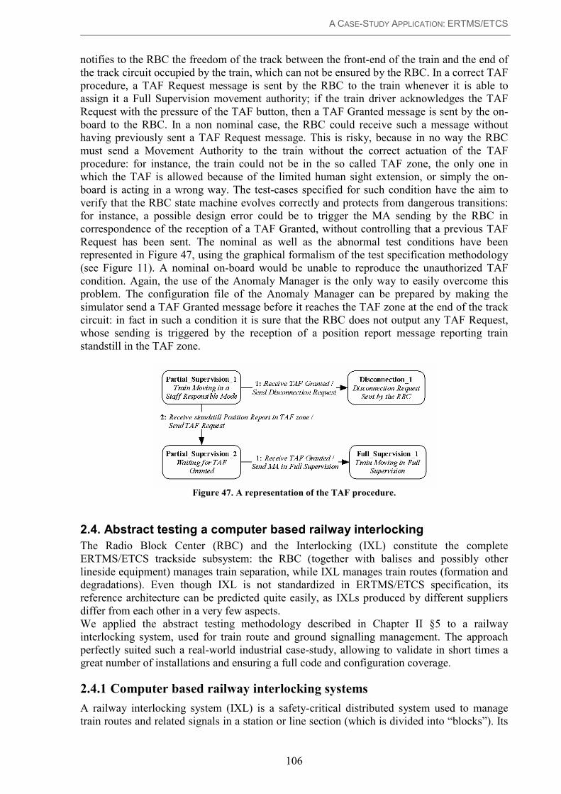
A CASE-STUDY APPLICATION: ERTMS/ETCS
106
notifies to the RBC the freedom of the track between the front-end of the train and the end of
the track circuit occupied by the train, which can not be ensured by the RBC. In a correct TAF
procedure, a TAF Request message is sent by the RBC to the train whenever it is able to
assign it a Full Supervision movement authority; if the train driver acknowledges the TAF
Request with the pressure of the TAF button, then a TAF Granted message is sent by the on-
board to the RBC. In a non nominal case, the RBC could receive such a message without
having previously sent a TAF Request message. This is risky, because in no way the RBC
must send a Movement Authority to the train without the correct actuation of the TAF
procedure: for instance, the train could not be in the so called TAF zone, the only one in
which the TAF is allowed because of the limited human sight extension, or simply the on-
board is acting in a wrong way. The test-cases specified for such condition have the aim to
verify that the RBC state machine evolves correctly and protects from dangerous transitions:
for instance, a possible design error could be to trigger the MA sending by the RBC in
correspondence of the reception of a TAF Granted, without controlling that a previous TAF
Request has been sent. The nominal as well as the abnormal test conditions have been
represented in Figure 47, using the graphical formalism of the test specification methodology
(see Figure 11). A nominal on-board would be unable to reproduce the unauthorized TAF
condition. Again, the use of the Anomaly Manager is the only way to easily overcome this
problem. The configuration file of the Anomaly Manager can be prepared by making the
simulator send a TAF Granted message before it reaches the TAF zone at the end of the track
circuit: in fact in such a condition it is sure that the RBC does not output any TAF Request,
whose sending is triggered by the reception of a position report message reporting train
standstill in the TAF zone.
Figure 47. A representation of the TAF procedure.
2.4. Abstract testing a computer based railway interlocking
The Radio Block Center (RBC) and the Interlocking (IXL) constitute the complete
ERTMS/ETCS trackside subsystem: the RBC (together with balises and possibly other
lineside equipment) manages train separation, while IXL manages train routes (formation and
degradations). Even though IXL is not standardized in ERTMS/ETCS specification, its
reference architecture can be predicted quite easily, as IXLs produced by different suppliers
differ from each other in a very few aspects.
We applied the abstract testing methodology described in Chapter II §5 to a railway
interlocking system, used for train route and ground signalling management. The approach
perfectly suited such a real-world industrial case-study, allowing to validate in short times a
great number of installations and ensuring a full code and configuration coverage.
2.4.1 Computer based railway interlocking systems
A railway interlocking system (IXL) is a safety-critical distributed system used to manage
train routes and related signals in a station or line section (which is divided into “blocks”). Its

A CASE-STUDY APPLICATION: ERTMS/ETCS
107
development and validation process must respect international safety norms [31]. Modern
IXL are computer based and feature a high number of functional requirements, thus making
them very complex. The verification and validation (V&V) process of such system consists in
a set of time consuming activities (hazard-analysis, code inspection, structural testing, etc.),
among which functional testing is undoubtedly the most important one, in terms of budget and
criticality. Moreover, IXL installations are different from each other; therefore, V&V consists
first in verifying the generic software application, and then the specific one. However, while
an abstract test-suite can be developed on the basis of the Generic Application (and then of
system functional specification), in order to verify the specific application the former test-
suite must be instantiated, according to the configuration of the installation under test.
Clearly, this need exactly fits the purpose of the presented abstract testing approach.
Traditionally, such an activity was performed by hand, with evident disadvantages in terms of
required effort and correctness of results.
A computer based IXL is composed of the following entities:
- a safety-critical centralized elaboration unit (let us indicate it with CPU), which is meant to
run the control software (processes and configuration);
- a Man Machine Interface (MMI), composed by a display and a functional keyboard which
allow the set and visual control of train routes;
- a Communication Computer (CC), used to manage the communication via a Wide Area
Network (WAN) with a (distant) central Automation System, also providing remote route
management, and possibly adjacent IXL;
- a set of Track Circuits (TC), used to detect if a train is occupying the route;
- a set of Switch Points (SP), used to form train route;
- a set of Light Signals (LS), used to notify to train drivers route status.
The IXL configuration associates each possible route to its related physical control entities:
TC, SP and LS.
A slightly simplified architecture of an IXL is reported in Figure 48(a).
Briefly, an IXL is basically used to manage route formation commands coming from a local
human operator (using the MMI) or a remote operator (using the AS). When a command is
received, the CPU controls its actability by checking the status of all involved entities, either
physical (TC, SP and LS) or logical (e.g. block orientation, line out of service, station
emergency, etc.). If route formation command is actable, then Switch Points are moved
accordingly. A route can also be formed in a degraded mode, in which route integrity can not
be assured because a check failed on a Track Circuit which is not clear or a Switch Point out
of control. These degradations reflect on route integrity status, which have to be properly
notified by multi-aspect Light Signals. Moreover, the system has also to manage the change
of route status when a train passes on it, until the liberation of the route. The state machine
associated to a route is quite complex: for the sake of simplicity, we will not describe it in
detail.
For our purposes, it is important to distinguish first of all between sensor and actuator entities
in an IXL. Clearly, Track Circuits can be considered as Sensors, as they are only used to
detect train position. Switch Points and Light Signals are instead Actuators, because they are
the actors of system control actions. The interface for route setting and monitoring, finally,
can be considered both as a Sensor, as it receives commands, and an Actuator, as it displays
outputs; analogously for the WAN interface. Another option, which is equivalent in theory but
could be advantageous in practice, is to consider the effects of MMI and WAN interfaces
directly on system state: intuitively, moving an input variable into a state variable is always
possible and does not necessarily impact on test accuracy.

A CASE-STUDY APPLICATION: ERTMS/ETCS
108
Now, let us define a possible IXL software architecture, using an object oriented design,
which we will use as a reference for our abstract testing application. Control processes will be
associated to each physical control entity (TC, SP, LS), thus obtaining:
- TC_Process, dealing with Track Circuit status (clear, occupied, broken, etc.);
- SP_Process, managing Swich Point status (straight, reverse, moving, out of control,
etc.) and operations (move_straight, move_reverse, etc.);
- LS_Process, aimed at controlling Light Signals’ status (green, red, yellow, flashing
yellow, etc.)
Furthermore, logic processes have to be defined for each logical control entity, thus obtaining:
- Route_Process, managing route status and control actions;
- Line_Process, managing out of service conditions, temporary speed restrictions, etc.;
- Block_Process, managing logical block orientation;
- LeftIXL_Process (managing data received by left adjacent IXL)
- etc.
Also Sensor type processes, if implemented according to object orientation, shall feature the
operations needed to access the status of their attributes.
An IXL will then feature a real-time kernel scheduling the above mentioned processes. In case
of the ASF Interlocking system, there exists a Logic Manager used to interpret and schedule
processes written in an application specific logic language (see §2.2 for a brief description of
its syntax), which allows for a sort of object orientation, even though not being specifically
object oriented (see Figure 48(b)). Moreover, a separate and well defined system
configuration will allow customizing the IXL to each specific installation (e.g. Manchester
railway station). In ASF implementation, the configuration database is of a relational type,
featuring tables containing “lists of entities” and “lists of linked entities”, expressing the
interrelationships between logic and physical control processes; such lists are used to perform
queries in order to determine the associations needed for the system to work and which
abstract testing is based on (they basically correspond to Sensor/Actuator_Association_Lists
referred to in Figure 9). Finally, the output state of the CPU is copied in a “state of entities”
database at each elaboration cycle, with attributes being primary keys, thus significantly
simplifying output state checking, as explained in previous section.

A CASE-STUDY APPLICATION: ERTMS/ETCS
109
(a)
(b) Figure 48. An IXL scheme (a) and related control software architecture (b).
2.4.2 Application of the abstract testing methodology
A possible approach in verifying an IXL from a system level point of view consists in the
following steps:
- Functional testing of the control software and measure of code coverage;
- Static verification of the configuration, using proper support tools;
- Acceptance testing regarding the verification of most significant railway logic
conditions.
While quite effective, such an approach does not guarantee dynamic configuration coverage.
In other words, control software is tested dynamically over a little part of a specific
configuration, until code coverage is considered satisfactory, but there is no evidence that the
integration of generic control logic and configuration is correct for the specific installation, as
the configuration is exhaustively verified only statically. Clearly, a dynamic black-box testing
of the specific installation, ensuring both code and configuration coverage, represents the
safest approach, also considering that installations can be very different one from each other,
thus possibly stimulating the control software with untested combination of inputs (refer to
[121] for a brief introduction to the hazard-analysis of railway control systems). However, an
extensive system testing based on such a criterion would be difficult and time consuming,
almost unfeasible using traditional approaches. This is where abstract testing comes in help,
by automating most of the work needed to achieve such objective.
In previous section, we showed the general architecture of an IXL and how it can be mapped
on the general scheme of Figure 9. This mapping being possible, the application of the
algorithm in its general form to our case-study reveals quite straightforward. In order to see,
in particular, how the algorithm applies to a specific abstract test-case, let us consider the
following requirement:
“When the IXL receives a route formation command it has to check the following
conditions:
All TC associated to the route must be clean
All SP associated to the route must be controlled
The LS associated to the route must be controlled

A CASE-STUDY APPLICATION: ERTMS/ETCS
110
If such conditions are fulfilled, then SPs have to be moved accordingly, route LS shall
be set to GREEN and Route Status has to be set to Integer”20
.
The requirement can be tested using the following abstract test-case (r represents a generic
route):
- Input State:
Route r TC Status = Clean
Route r SP Status = Controlled
Route r LS Status = Controlled
- Input:
MMI Input: Route r Formation Command
- Output:
Route r SP Output = Positioned according to r
Route r LS Output = GREEN
- Output State:
Route r Status = Integer
For such an abstract test-case, the algorithm:
- Step 1: Selects all input states satisfying the Si condition specified in the test-case. In
other words, all combinations of TC, SP and LS statuses associated to each configured
route have to be set to the specified values; for the specific test-case, there exists exactly
one combination of such values for each possible route, corresponding to a nominal
system state (e.g. the idle state following system start-up);
- Steps 2-4: Stimulates the IXL via the (simulated) MMI with the specific route formation
command; as only one command is possible for each route, the SEN and I conditions will
select exactly one sensor and one input for each input state;
- Steps 5-6:
Checks that all SP are positioned according to the specific route; the actuator selection
routine applies to switch points of the specific route: condition ACT will read as
follows “Actuators SP whose Routes attribute contains r” (SP are associated to more
than one route); condition O will be “Positioned according to r”;
Checks that the specific route status is set to GREEN: the check for LS output is
analogous to the one described for SP (see point 0 above);
- Steps 7-13: Checks that output status satisfy the So condition, that is “Route r Status =
Integer”. As attributes are not duplicated into different objects and a “state of entity”
dynamic database is available, such check consists in a simple database access, verifying
that “Route_Status_r” (primary key) is set to the value “Integer”.
Clearly, the algorithm will produce as many physical tests as the number of possible routes
which are configured in the IXL. The example is straightforward, as it usually happens when
dealing with nominal tests. A possible negative test, related to the previous one, corresponds
to the following statement:
“[…] If any of the conditions listed above is not fulfilled, then route command must
not be accepted”.
20 In a real IXL, the correct execution of a switch movement command must be verified before setting the signal
to GREEN (in other words, SPs feature additional sensors).

A CASE-STUDY APPLICATION: ERTMS/ETCS
111
In such a case and without adopting any reduction criterion on Si, we would have a significant
increase in the number of generated physical tests. In fact, for each route the combinations of
input states impeding the correct formation of the route are numerous, and all of them should
be tested.
In order to implement abstract testing in practice and to perform test automation, the
transformation algorithm has to be translated into an executable language (e.g. “C”), and its
output must correspond to a test script whose syntax is interpretable by the specific simulation
environment. In our experience with the verification of IXL systems, we developed a series of
tools and integrated them into a cohesed functional testing framework (an example is
described in [55]), which deeply facilitated the implementation of abstract testing, according
to the general guidelines described in this section.
3. Multiformalism analyses for the availability evaluation of ERTMS/ETCS
In this section we describe the application to ERTMS/ETCS of the multiformalism
methodologies presented in Chapter III.
This section is based on some of the case-study results published in [54] and [56].
3.1. Evaluating the availability of the Radio Block Center of ERTMS/ETCS against complex repair strategies by means of Repairable Fault Trees
In order to prove the power of the RFT approach, we evaluated the impact of different repair
policies on the availability of a critical computer which constitutes the heart of the
ERTMS/ETCS trackside (ground) subsystem: the Radio Block Centre (RBC). Being a
complex repairable system, the RBC constitutes the ideal case-study to show the practical
benefits of the RFT formalism. Furthermore, at the best of our knowledge no maintainability
study has been performed on the RBC (at the time we are writing).
Figure 49. A RBC centered view of ERTMS/ETCS level 2.
3.1.1 The importance of RBC availability in ERTMS/ETCS
Figure 49 shows RBC interactions at the level 2 ERTMS/ETCS implementation. At this level,
the Radio Block Center (RBC) is the most important ERTMS/ETCS subsystem, as it is
responsible for guaranteeing a safe outdistancing between trains by managing the information
received from the on-board subsystem (by means of the GSM-R network) and from the
Interlocking (IXL) subsystem (by means of a dedicated Wide Area Network, WAN) in order
to compute and send to the trains their movement authorities, which represent the distance the

A CASE-STUDY APPLICATION: ERTMS/ETCS
112
trains are allowed to cover in safe conditions. The positioning information received from the
trains allows the RBC to locate them on its internal route representation, while the track status
received from the IXL allows the RBC to compute the information related to track occupancy
status. Finally, on the basis of such information, the RBC computes the movement authorities
to be transmitted to the trains via GSM-R. Therefore, the unavailability of a RBC is critical, as
there is no way for the signaling system to work without its contribution. In case of a RBC
failure, all the trains under its supervision (typically more than 5) would be compelled to
brake and proceed in a staff responsible mode, and this would lead to the most critical
ERTMS/ETCS (safe) failure. Most of the functions that an ERTMS/ETCS system has to
manage are allocated on the RBC, which is the most complex subsystem.
3.1.2 RBC availability requirements and hardware architecture
As introduced in Section 1.4, the ERMTS/ETCS standard requires compliance with specified
RAMS (Reliability Availability Maintainability Safety) requirements [149]. RAM
requirements specify for the RBC a maximum unavailability of 10-6 (see [149], §2.3.3), whose
fulfillment has to be properly demonstrated. We largely mentioned that international
standards and guidelines for railway V&V processes explicitly advocate the use of formal
methods in order to demonstrate the fulfillment of RAMS requirements. As for any mission
critical computer system, the RBC must be designed to be highly fault-tolerant and easily
maintainable on-line, without service interruption. The very high level of availability required
for the RBC can be obtained by balancing the reliability of the used components, the degree
of redundancy of the system and the adopted maintenance strategies. Using high reliable
components is very expensive, as development costs increase with reliability in a more than
linear way. This justifies the use of COTS (Commercial Off The Shelf) components, which
are not very reliable but can be redundant and have the advantage to highly reduce
development times and costs. Increasing too much the redundancy of the system, however,
also increases system complexity, which brings a lot of design and validation issues in safety-
critical real-time systems. Double or triple redundancy is usually adopted depending on the
specifications: one exception consists in the computing sub-system, which is usually based on
a 2oo3 (2 out of 3) voting. Such a configuration is also known as Triple Modular Redundant
(TMR) computing subsystem and it is a cheaper and more available alternative to the
redundant 2oo2 (2 out of 2) configuration (the voting is always necessary for safety reasons).
In order to build a proper model of the RBC, in the following a reference architecture is
described in its structure, components and reliability parameters. The computing subsystem
can be made up by three commercial CPU-RAM cards and a redundant FPGA based voter in
a TMR configuration. The GSM-R and WAN communication subsystems are also chosen as
COTS. Three commercial power supplies and a redundant standard backbone (used as the
main system BUS) complete the RBC configuration, which therefore does not require any
specifically designed component. RBC architecture is represented in the class diagram of
Figure 50. The reference values of component reliability parameters, chosen from the data-
sheets of commercial devices, are listed in Table 5.
Figure 50. Class diagram of the RBC.

A CASE-STUDY APPLICATION: ERTMS/ETCS
113
Table 5. COTS reliability values.
As in many other contexts, the balancing between different design choices is a matter of
trade-offs which are often quite difficult to manage. From the above considerations it is clear
that no many degrees of freedom are available for the designer (i.e. reliability engineer) in the
industrial practice and thus maintenance policies become a fundamental aspect to concentrate
on, as they directly impact on system availability and are more easily manageable than many
other factors. This is the reason why it is important not only to evaluate the impact of design
choices and reliability parameters on the RBC availability, but also to concentrate on the
maintenance policies. ERTMS/ETCS gives only qualitative suggestions for preventive
maintenance, while the upper bounds for corrective maintenance intervention times are very
high (not more than 2 hours; see [149] §2.2.2.3.2 and §2.2.2.3.3). There are no other
restrictive requirements for the maintainability parameters and this leaves a lot of freedom in
designing and dimensioning repair policies. The assumptions made about the nominal values
of repair parameters (MTTR) are given in Table 6; these values are chosen on the basis of
empirical considerations about component accessibility, mean substitution times and restart
delays.
Table 6. Reference parameters for repair.
3.1.3 Modeling and analysis
In order to compare the effects of different repair strategies, the system has been modeled by
means of the RFT formalism. Several RB have been designed as described in Chapter III §2,
introducing slight differences with respect to the general framework defined in [37]. As first,
starting from the RBC architecture, the RFT model of the RBC has been created following
usual FTA techniques. Then, different RBs have been applied to the RBC in order to evaluate
the achievable improvements on overall system availability. The repair policies differ the in
allocation and number of repair resources. To obtain an upper bound, a model with unlimited
resources and a complete independence among repair actions is used to evaluate the ideal
(best) achievable unavailability of the RBC, given reference MTBF and MTTR values. Then,
a complex repair policy is applied with a variable number of repair resources, including the
case of non-continuous availability of the resource. A further study is performed on the
comparison of the aforementioned repair policies. Moreover, the effects of (fixed) priority
schemas on the repair policy are evaluated, assuming a single repair resource. Finally, in the
last part of this section we show how to use the RFT formalism to tune component reliability
parameters given system specifications.

A CASE-STUDY APPLICATION: ERTMS/ETCS
114
The reference repair policy and the upper bound for availability
The basic idea behind the reference repair policy is that using both on-line and off-line repair
approaches is a good trade-off between the required parameters for components and the global
MTTR. In the reference repair policy, two basic repair mechanisms are used: the on-line
repair is triggered whenever a single component of the RBC fails, before the fault generates a
system failure, while a (higher priority) off line repair restores the minimal number of
required components to remove system failure whenever a system failure happens, in order to
reduce the system down time. Such a repair strategy (in which the same repair resources are
shared between the two mechanisms) gives the single subsystems a higher availability and
achieves a fast system restore by polling one by one faulty subsystems and removing only the
minimal fault set. In each RB it is embedded a repair action, performed on a certain
subsystem (component by component) by using a repair resource (e.g. a maintainer) in a
certain time (i.e. component MTTR). The repair action is triggered by a condition verified by
the subsystem (e.g. a fault of one of the components in the subsystem).
Figure 51. The RBC RFT general model.

A CASE-STUDY APPLICATION: ERTMS/ETCS
115
Figure 52. The GSPN model of the RFT.
The RFT for the RBC is showed in Figure 51; its GSPN translation is depicted in Figure 52.
For each subsystem and for the global system there are RBs, properly connected to the events
that contribute to their triggering. Each RB also reports the priority level with which it is
activated in case of conflicts on the triggering conditions (here the global RB has priority on
the local RBs when in conflict for a repair resource).
The reference unavailability measure with which we compare the quality of the various repair
policies is obtained by setting the number of resources to infinite (that is, giving independent
and infinite resources to each RB)21
. Given the reference parameters in Table 5 and Table 6,
our analysis gives an overall unavailability of 1.304*10-6. The only way to improve this limit
is to modify component parameters (MTTR and MTBF).
Effects of available resources
In order to evaluate the effects of limited repair resources, two cases have been considered in
the model, with one and two shared resources respectively. Moreover, two further scenarios
have been considered in which resources are available only in the 50% and in the 10% of the
time respectively; this models a situation in which the repair personnel is part-time allocated
to the RBC (e.g. it is shared with other RBCs). Furthermore, the time ratio of attendance can
be composed of several rounds (e.g. the RBC has the resource for 50% of the time, sliced in
turns of 2 hours each), whose length impacts on availability. Results of these analyses are
listed in Table 7 and in Figure 53.
21 This scenario can be evaluated by means of a simple Fault Tree where availability values are used for
components instead of MTBF.

A CASE-STUDY APPLICATION: ERTMS/ETCS
116
Table 7. RBC unavailability with respect to resources.
Figure 53. RBC sensitivity to number and attendance of repair resources.
As from the results, it is evident that the number of resources gives a significant contribution
to the policy. The unavailability achieved using two resources is far better than using one
resource, and the result is comparable to the value achievable with infinite resources (the
difference is only 3%).
About the part-time attended repair policies, in which, to model a situation that prevents the
resource to be (continuously) available for RBs, the resource is inhibited for a given
percentage of the time, results show that as first the continuous availability of at least one
resource is critical for the overall availability of the system (for the 50% of presence in the
best turn there is a loss of one order of magnitude for unavailability). It is noticeable that
better results are obtained with shorter turns (that is, shorter unattendance periods), which
suggests that in case of resource sharing it is preferable a close sequence of attendance and
unattendance periods. Results in the 10% case are very poor, and should advice the need for a
higher expense on repair resources.
Finally, a more accurate analysis requires the evaluation of cost factors which are not possible
using the RFT formalism, together with considerations that are related to other ERTMS/ETCS
subsystems; in fact, a global analysis would help to understand whether the RBC
unavailability is a limiting factor or not (see next §3.2).
Effects of the policy
As mentioned above, the reference repair policy has two main contributes: an off-line and an
on-line repair action. In order to evaluate the opportunity of implementing both actions, it is
useful to evaluate the unavailability of the RBC when only the off-line repair action is
available. Since this action is implemented by a single repair resource and in this situation the
presence of a repair resource is only relevant and always necessary when the RBC fails, no
variation on resources is considered in the analysis for the alternate model. This RFT model is
simply obtained from the model in Figure 51 removing all the RBs but the top one.
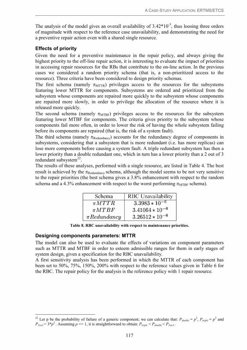
A CASE-STUDY APPLICATION: ERTMS/ETCS
117
The analysis of the model gives an overall availability of 3.42*10-3, thus loosing three orders
of magnitude with respect to the reference case unavailability, and demonstrating the need for
a preventive repair action even with a shared single resource.
Effects of priority
Given the need for a preventive maintenance in the repair policy, and always giving the
highest priority to the off-line repair action, it is interesting to evaluate the impact of priorities
in accessing repair resources for the RBs that contribute to the on-line action. In the previous
cases we considered a random priority schema (that is, a non-prioritized access to the
resource). Three criteria have been considered to design priority schemas.
The first schema (namely πMTTR) privileges access to the resources for the subsystems
featuring lower MTTR for components. Subsystems are ordered and prioritized from the
subsystem whose components are repaired more quickly to the subsystem whose components
are repaired more slowly, in order to privilege the allocation of the resource where it is
released more quickly.
The second schema (namely πMTBF) privileges access to the resources for the subsystem
featuring lower MTBF for components. The criteria gives priority to the subsystem whose
components fail more often, in order to lower the risk of having the whole subsystem failing
before its components are repaired (that is, the risk of a system fault).
The third schema (namely πRedundancy) accounts for the redundancy degree of components in
subsystems, considering that a subsystem that is more redundant (i.e. has more replicas) can
lose more components before causing a system fault. A triple redundant subsystem has then a
lower priority than a double redundant one, which in turn has a lower priority than a 2 out of 3
redundant subsystem22
.
The results of these analyses, performed with a single resource, are listed in Table 4. The best
result is achieved by the πRedundancy schema, although the model seems to be not very sensitive
to the repair priorities (the best schema gives a 3.8% enhancement with respect to the random
schema and a 4.3% enhancement with respect to the worst performing πMTBF schema).
Table 8. RBC unavailability with respect to maintenance priorities.
Designing components parameters: MTTR
The model can also be used to evaluate the effects of variations on component parameters
such as MTTR and MTBF in order to esteem admissible ranges for them in early stages of
system design, given a specification for the RBC unavailability.
A first sensitivity analysis has been performed in which the MTTR of each component has
been set to 50%, 75%, 150%, 200% with respect to the reference values given in Table 6 for
the RBC. The repair policy for the analysis is the reference policy with 1 repair resource.
22 Let p be the probability of failure of a generic component; we can calculate that: Pdouble = p
2, Ptriple = p
3 and
P2oo3 = 3*p2 . Assuming p << 1, it is straightforward to obtain: Ptriple < Pdouble < P2oo3 .

A CASE-STUDY APPLICATION: ERTMS/ETCS
118
Table 9. RBC unavailability with respect to on-line and off-line MTTR.
Figure 54. RBC sensitivity to MTTR variations.
Table 9 and Figure 54. RBC sensitivity to MTTR variations. show the effects on RBC
unavailability of variations of the parameters. Considering the operation needed to replace
components, they have been grouped in two sets sharing the same MTTR: the Bus and FPGA
components have MTTR-BF, all other components have MTTR-Card; moreover, the off-line
repair policy has MTTR-OffLine, including all the operations needed to check, fix and restart
the system. While these parameters vary, all the other parameters are kept to reference values.
MTTR-OffLine improvements are obviously very effective because as they have a direct
impact on system down-time; however, they are limited by the time to diagnose and to restart.
More relevant results have been obtained for MTTR-Card and MTTR-BF. In both cases, the
increase in unavailability is linear in the reference range, but the higher marginal contribution
is given by MTTR-Card variations. MTTR-Card (which includes the time needed to
physically access failed components, the time to reinstall them, the time for reintegration of
the repaired component in the system) can be lowered by technological means, but also acting
on component (i.e. LRU) accessibility in the RBC rack and improving operational procedures.

A CASE-STUDY APPLICATION: ERTMS/ETCS
119
Table 10. RBC sensitivity to MTBF variations.
Designing components parameters: MTBF
Another sensitivity analysis has been performed which the MTBF of each component has
been set to the 50% and 20% with respect to the reference values. The repair policy for the
analysis is again the reference policy with one repair resource. Table 10 shows the effects on
the RBC unavailability of parameter variations. In the table, three components have been
considered to investigate which of them can be the limiting factor in the architecture and
which of them can possibly be substituted by a less reliable (and less expensive) one. Only
two variations are shown in the table for the most significant components. As in the other
cases, the reference repair policy is applied with one repair resource, and in each of the cases
summarized in Table 10; the other parameters are kept to their reference values. It is visible
that the system is completely indifferent to variations of the FPGA MTBF in the reference
range, while the CPU board is critical. In fact, by halving the MTBF, the RBC unavailability
looses one order of magnitude, while a double MTBF for the CPU board gives the system an
unavailability that is close to the case in which two repair resources are used (the difference is
29%, while the difference given by the additional resource with respect to the reference case
is 60%).
Overall comparison
The variety of possible interventions whose effects can be evaluated on the model gives the
designer wide freedom in choosing the best combination of factors leading to the necessary
availability for the system. In our case, the best combination (not considering cost factors and
discussion about lower bounds for the off line MTTR) is given by using two repair resources,
a πRedundancy policy for resource allocation and a 50% factor for the off-line MTTR. In these
conditions, the RBC unavailability is 6.736*10-7, improving the infinite resources result with
reference parameters by a 48%.
Figure 55. Comparison of different design choices.

A CASE-STUDY APPLICATION: ERTMS/ETCS
120
An overall comparison of the best results obtained by the analysis is reported in Figure 55.
The graph shows the improvements for RBC unavailability for each of the most significant
(effective) techniques. Of course, the optimal choice depends on the availability of resources
and on the cost of variations: nevertheless, the graph is a valid reference to evaluate effects of
different trade offs between resources, quality of components and repair efficiency.
3.2. Evaluating system availability of ERTMS/ETCS by means of Fault Trees and Bayesian Networks
Critical control systems require proper techniques to predict their failure rate since early
design stages, in order to fulfill dependability requirements and minimize development costs.
In Chapter III, Bayesian Networks have been shown to be suitable to model structural
reliability aspects, extending the modeling power of Fault Trees and featuring a better solving
efficiency with respect to Petri Nets. In this section, we exploit the Fault Tree and Bayesian
Network formalisms, as described in Chapter III §3, in order to perform a structural
availability analysis of ERTMS/ETCS. As largely mentioned above, ERTMS/ETCS is a
complex real world case study, featuring a distributed heterogeneous architecture with strict
availability requirements. On the basis of such requirements and of the hypothesized system
reference architecture, we studied structural availability by instantiating models with realistic
reliability parameters and performing a series of sensitivity analyses in order to highlight
design trade-offs. By evaluating and integrating sub-models using a compositional approach
we both obtained several interesting results and showed the effectiveness of a combined use
of Fault Trees and Bayesian Networks in dealing with structural reliability analyses of train
control systems.
A structural reliability model of ERTMS/ETCS with respect to system level failures due to
casual hardware faults cam be represented by means of composition operators with the
semantic of connectors (see Chapter III §4) in Figure 56. This structure is general enough to
model any failure mode and its semantics only depends on the instantiation of composition
operators. The structure of Figure 56 clearly highlights the advantages of composition based
modeling, with the possibility of defining and reusing libraries of standard components.
Figure 56. ERTMS/ETCS composed hardware failure model.
It should be noted that operators can not only perform copy of results or AND / OR / “M-out-
of-N” computations, because more failure modes are addressed (namely Immobilizing,

A CASE-STUDY APPLICATION: ERTMS/ETCS
121
Service and Minor failures), as it will be clear in next sections, in which such composition
will be performed “by hand”.
3.2.1 The Lineside subsystem: modelling and evaluation
Lineside model structure
The Lineside subsystem at ERTMS/ETCS L2 is not implementation specific, so the
considerations presented in this section are very general. In fact, given track related
parameters (i.e. track length and BG interdistance, which impact on total BG number), design
freedom only regards the dimension of reliability related parameters (i.e. MTBF, MTTR and
redundancy). In particular, redundancy reflects on the number of balises for each group,
which can vary from 2 to 8, according to the specification (we explicitly neglect the case of
single balise groups, as they do not allow to detect train direction, so they are never used in
current applications of the standard). Finally, we remark that ERTMS/ETCS RAM
specification for constituents requires UBAL < 10-7 (e.g. a combination of MTBF=10
7h and
MTTR=1h). In our analysis, we provided a variation interval for Lineside reliability
parameters in order to show that less reliable balises used in redundant groups are able to
easily fulfil system level availability requirements at a less cost (we will consider the impact
of Lineside availability on overall system availability in Section 6). In particular, we assumed
the Lineside is responsible for an Immobilising Failure whenever two adjacent BGs fail, as
such an event causes the train to apply the emergency brakes as the so called “balise linking
error reaction” in most system implementations. The Fault Tree model for the Lineside is
depicted in Figure 57 (BG structure, being the same for all groups, is only explicited for the
first one).
BG1.1 fail
BG1.2 fail
AND
OR
Track 1
Lineside
failure
OR
BG1.2 fail
BG1.3 fail
AND
BG1.(N/2-1) fail
BG1.N/2 fail
AND
...
BG2.1 fail
BG2.2 fail
AND
Track 2
OR
BG2.2 fail
BG2.3 fail
AND
BG2.(N/2-1) fail
BG2.N/2 fail
AND
...
BaliseM fail
Balise1 fail
... 2ooM
Figure 57. Fault Tree model of the Lineside subsystem.
Lineside model parameters
The description and variability interval for parameters is presented in Table 11. The
variability interval of the total number of balise groups has been chosen considering: realistic
track lengths from 100Km to 400Km, an average BG inter-distance of about 1Km, and both
track directions.

A CASE-STUDY APPLICATION: ERTMS/ETCS
122
PARAMETER DESCRIPTION MIN MAX STEP
MBG Number of balises for each group 2 8 1
NBG Total number of balise groups 200 800 200
MTBFBAL Mean Time Between Failures for each balise [h] 2.5 105 1.5 106 2.5 105
MTTRBAL Mean Time To Repair for each balise [h] 0.5 2.5 1
UIF-LNS Lineside system unavailability with respect to Immobilising Failures
Table 11. Lineside model parameters.
Lineside model evaluation
Selected results of the analyses are shown in Table 12 (as aforementioned, the only significant
failure mode for the Lineside leads to an Immobilising Failure). Table 12 suggests that BGs
constituted by more than 2 balises are over-dimensioned with respect to ERTMS/ETCS
availability requirements: this result formally justifies the practical choice of adopting groups
constituted by just two balises in all current projects. The possibility to adopt BG of up to 8 (!)
balises seems therefore completely useless, as the only reason to do this would be using very
low reliable balises, which is obviously not convenient, as frequent on-the-track interventions
are difficult and costly. As for the other results, almost any combination of Lineside
parameters produce acceptable results, with most of them (not all shown in the table) leading
to UIF-LNS<10-8. The only results requiring attention are the ones corresponding to the worst
combinations of parameters: maximum track length, lowest balise reliability, highest time to
repair: even in such worst conditions, the result of UIF-LNS≈10-7 is perfectly compatible with
the order of magnitude of the other ERTMS/ETCS subsystems, as it will be shown in the
following sections. In fact, other ERTMS/ETCS subsystems (e.g. EVC, RBC, etc.) feature a
similar unavailability, but in a typical installation they are usually required in a number which
is more than one. However, the mentioned worst case corresponds to a balise unavailability:
UBAL= 1−MTBFBAL/( MTBFBAL+MTTRBAL)=1−2.5*105/(2.5*10
5+2.5)=10
-5,
which is two orders of magnitude higher than the 10-7
value stated by RAM specification for
constituents (see
Table 4), thus justifying the convenience of a system level approach. Finally, the Lineside
results presented above justify the possibility to neglect the Lineside subsystem contribution
in a global system availability analysis when a proper choice of parameters is performed.
MBG NBG MTBFBAL MTTRBAL UIF-LIN
0.5 h 3.1840*10-9
1.5 h 2.8655*10-8
2.5 h 7.9598*10-8
2.5 105 h
2.5 h 1.9900*10-8
200
106 h 2.5 h 4.9750*10-9
400 7.5 105 h 1.5 h 6.3839*10-9
0.5 h 1.2784*10-8 2.5 105 h
2.5 h 3.1959*10-7
5.0 105 h 0.5 h 3.1960*10-9
2
800
106 h 1.5 h 7.1909*10-9
≥ 3 Any Any Any ≈ 0 (<< 10-10)
Table 12. A selection of Lineside results.
3.2.2 The On-board subsystem: modelling and evaluation
On-board model structure
We will realistically assume the On-board system is not repairable on-line, for the
unavailability of an on-board technician. Moreover, each On-board system only features a
failure mode related to availability. In other words, at any time the On-board can only assume
two states: available (working in full operating mode) and unavailable. A Fault Tree model
based on components’ MBTF perfectly fit the required analysis. The FT model will comprise
all On-board components described in Section 2, in redundant configurations to avoid single
point of failures, plus the ones constituting the EVC elaboration subsystem (based on a basic
TMR architecture, as aforementioned). In particular, the EVC will feature: 3 CPU cards with

A CASE-STUDY APPLICATION: ERTMS/ETCS
123
dedicated memory; a redundant FPGA-based majority voter on CPU outputs; 3 redundant
Power Supplies (PS); a system BUS interconnecting all the peripherals. All ERTMS/ETCS
components are essential for correct on-board operation, and thus are connected to the Top
Event of the Fault Tree via an OR gate. The FT model for the On-board is depicted in Figure
58: the FT formalism is quite easy to read and thus self-explaining, so we are not going to
describe model details any further. To cause an Immobilising Failure due to the On-board
subsystems, at least two of them must fail, while for a Service Failure just one On-board
failure is sufficient.
PS1 fail
PS2 fail
PS3 fail
AND
OR
BUS1 fail
BUS2 fail
AND
PS fail
BUS fail
TMR fail
CPU1 fail
CPU2 fail
CPU3 fail
2oo3
ANDVoter1 fail
Voter2 fail
OR
RTM1 fail
RTM2 fail
ANDRTM fail
BTM1 fail
BTM2 fail
ANDBTM fail
DMI1 fail
DMI2 fail
AND DMI fail
ODO1 fail
ODO2 fail
ANDODO fail
TIU1 fail
TIU2 fail
AND TIU fail
On-board
failure
CPU fail
Voter fail
Figure 58. Fault Tree model of the On-board subsystem.
On-board model parameters
For the EVC, Commercial Off The Shelf (COTS) components have been chosen, consulting
commercial datasheets. Such values should be considered only as orders of magnitude, to
have an idea of typical COTS reliability. For instance, Power Supply is chosen to be dual
redundant because typically it is less reliable than other components. For standard
ERTMS/ETCS devices (e.g. BTM, RTM, etc.), the basic MTBF values have been chosen in
accordance with specified RAM requirements for constituents; then their value has been
varied in a sensitivity analysis whose results will be described in next section. The chosen
parameters are reported in Table 13. With safe train headways of at least 15Km (considering
the train braking distance at a maximum speed of at least 300Km/h), the average number of
trains does not exceed 24 for typical track lengths (however, lower values are far more
probable, as high-speed railway lines are not so heavily loaded in practice).

A CASE-STUDY APPLICATION: ERTMS/ETCS
124
PARAMETER DESCRIPTION VALUE
NONB Total number of On-board systems 2-24
MTTRONB MTTR of the On-board 30’, 1h, 2h
MTBFCPU MTBF of the Processor-Memory Card 1.35*105 h
MTBFBUS MTBF of system Bus 2.25*105 h
MTBFVOT MTBF of each FPGA based Voter 3.33*108 h
MTBFPS MTBF of Power Supply 5.50*104 h
MTBFRTM MTBF of the Radio Transmission Module 106 h
MTBFBTM MTBF of the Balise Transmission Module 108 h
MTBFODO MTBF of the on-board Odometer 107 h
MTBFTIU MTBF of the Train Interface Unit 107 h
MTBFDMI MTBF of the Driver Machine Interface 107 h
MTBFONB MTBF of a single On-board system
MTBFIF-ONB MTBF of the On-board system with respect to Immobilising Failures
MTBFSF-ONB MTBF of the On-board system with respect to Service Failures
Table 13. On-board model parameters.
On-board model evaluation.
The results of On-board model evaluation have been obtained fixing COTS’ MTBF values
(which are given by their specification) and varying the MTBF of ERTMS/ETCS
components, as the latter have to be developed ex novo. In particular, to better understand the
impact of ERTMS/ETCS components’ reliability on On-board system reliability, we
performed a sensitivity analysis whose results are shown in Table 14 (with reference to a
single On-board system). Row headings represent the scaling factors on variable parameters
for the sensitivity analysis (e.g. Scale 0.1 for RTM means MTBF*RTM = 0.1*10
6 h = 10
5 h).
The overall On-board system sensitivity to ERTMS/ETCS components’ reliability is quite
low when MTBF scales up or down of only one order of magnitude, as the EVC constitutes
the main reliability bottleneck; when the reliability of ERTMS/ETCS components is scaled of
two or more orders of magnitude, instead, the impact on MTBFONB is more significant. By
simply observing model structure, with the hypothesized reference architecture and in a Level
2 implementation, it does not appear to be any reason to assign a higher reliability to certain
On-board components, as their influence only depends on their reference value and not on
structural aspects (probably, the specification choice of differentiating them is related to the
possibility for the On-board to “fall-back” into the lower ERTMS/ETCS Level 1; such a
possibility has not been implemented in any real project). Therefore, despite of component
RAM specification, our system level analysis for an ERTMS/ETCS Level 2 implementation
suggests a balanced choice of MTBF for ERTMS/ETCS components; e.g. all components’
MTBF = 106
h implies MTBFONB = 6,3825*10
4 h. Finally, Table 15 shows the impact of
MTTRONB and of the number of trains on overall On-board reliability and availability (only a
selection of results is reported). Our analysis shows that the On-board MTBF requirements of
Table 4 are not respected by our reference architecture, even with a low number of trains;
however, such requirements are hardly fulfilled even by completely redundant On-boards
using very reliable components. Therefore, they seem over dimensioned considering real EVC
implementations (which constitute the limiting factor to reliability). Fortunately, from a
system level point of view, it is sufficient to reason in terms of unavailability, whose results
for the On-board are also reported in Table 15 and seem compatible with system level
requirements which will be used in the global analysis of Section 6.
SCALE MTBFONB
10 6.4776*104
1 6.4769*104
0.1 6.4195*104
0.01 4.4182*104
0.001 0.6885*104
Table 14. Results of the On-board sensitivity analysis.

A CASE-STUDY APPLICATION: ERTMS/ETCS
125
MTTRONB NONB MTBFSF-ONB MTBFIF-ONB USF-ONB UIF-ONB
2 3.1913*104 9.5738*104 1.5667*10-6 5.2223*10-6
4 1.5956*104 3.7232*104 3.1335*10-5 1.3429*10-6
6 1.0638*104 2.3403*104 4.6999*10-5 2.1364*10-5
12 5.3188*103 1.1121*104 9.3997*10-5 4.4958*10-5
30’
24 2.6594*103 5.4344*103 1.8798*10-4 9.1998*10-5
1h 6 1.0638*104 2.3403*104 9.3994*10-5 4.2728*10-5
2h 6 1.0638*104 2.3403*104 1.8797*10-4 8.5452*10-5
Table 15. On-board unavailability with respect to MTTR and number of trains.
3.2.3 The Trackside subsystem: modeling and evaluation
Trackside model structure
Most of the considerations already done about the architectural model of the EVC can be
applied to the Radio Block Center, with the following two differences: 1) instead of On-board
ERTMS/ETCS components, the RBC only features two communication interfaces (GSM-R
and WAN); 2) the RBC is a repairable system, which can be maintained on-line by a
dedicated technician. Therefore, while model structure remains substantially the same, the
computation will be performed with respect to components’ availability instead of MTBF.
The Fault Tree formalism still suits such kind of analysis, in the infinite repair resources
assumption: when a failure occurs to a component, the repair action starts immediately and
finishes after a Mean Time To Repair which is independent from concurrent failures and does
not account for possible system restart times (we assume them negligible; for more articulated
maintenance policy modelling, refer to §3.1). The RBC Fault Tree model is depicted in Figure
59. Just like the Lineside, the only failure mode for a RBC leads to an immediate system
Immobilizing Failure, as the number of trains meant to be managed by each RBC is at least 2.
Therefore, with respect to IFs, the Trackside can be modelled by a simple OR gate connecting
all RBCs installed on the track.
PS1 fail
PS2 fail
PS3 fail
AND
OR
BUS1 fail
BUS2 fail
AND
PS fail
BUS fail
TMR fail
CPU1 fail
CPU2 fail
CPU3 fail
2oo3
ANDVoter1 fail
Voter2 fail
OR
GSM1 fail
GSM2 fail
AND GSM-R fail
WAN1 fail
WAN2 fail
ANDWAN fail
RBC
failure
CPU fail
Voter fail
Figure 59. Fault Tree model of the Radio Block Center.
Trackside model parameters
Refer to Section 3.2.2 for explanation about the COTS components used in the computing
subsystem (the chosen MTBF are the same). For GSM-R and WAN interfaces, COTS
components are used, too. The MTTR is assumed to be the same for all components, each of
which is easy accessible and hot-replaceable. The MTTR variation set consists in typical
values for supervised systems: 5, 10 and 30 minutes (the latter can correspond to a system
with less easily accessible components or more hardly diagnosable faults).

A CASE-STUDY APPLICATION: ERTMS/ETCS
126
PARAMETER DESCRIPTION VALUE
NRBC Total number of Radio Block Centres 1-5
MTBFCPU MTBF of the Processor-Memory Card 1.35*105 h
MTBFBUS MTBF of system Bus 2.25*105 h
MTBFVOT MTBF of each FPGA based Voter 3.33*108 h
MTBFPS MTBF of Power Supply 5.50*104 h
MTBFGSM MTBF of GSM-R communication interface 1.75*105 h
MTBFWAN MTBF of WAN communication interface 4.00*105 h
MTTRRBC Mean Time To Repair (or replace) a RBC component 5’, 15’, 30’
Table 16. Trackside model parameters.
Trackside model evaluation
For the RBC, no MTBF requirement is given, so we can directly reason in terms of
availability. Table 17 reports the evaluated unavailability of the Radio Block Center with
respect to different repair times. Availability is related to reliability and maintainability
according to the well know formula: A=MTBF/(MTBF+MTTR). Therefore, the result of
strong dependence between URBC and MTTRRBC, shown in Table 17, is expectable and
underlines the importance of adopting efficient repair strategies and hot-spare components:
this allows satisfying the requirement on system availability (URBC<10-6) without using highly
reliable and expensive ad-hoc components. However, for the system level analysis we won’t
consider the poorly realistic result corresponding to the lowest MTTRRBC=1’, as we will show
that this is not necessary to satisfy the system level availability requirement. Finally, Table 18
shows the results about Trackside unavailability, assuming a realistic MTTRRBC=15’.
According to the results obtained, the number of RBC should be kept as low as possible;
however, other factors (e.g. performance requirements) constrain such a choice. As evaluated
for the On-board (see Section 4), it could be shown that the requirement MTBF-ITRK>3.5*108
h is largely over-dimensioned: we will simply neglect it and proceed to our system level
analysis.
MTTRRBC URBC
1’ 3.0182*10-7
5’ 1.5145*10-6
15’ 4.5454*10-6
30’ 9.0909*10-6
Table 17. RBC unavailability with respect to repair times.
NRBC UIF-TRK
2 9.0909*10-6
3 1.3636*10-5
4 1.8182*10-5
5 2.2727*10-5
Table 18. Trackside unavailability with respect to the number of RBCs.
3.2.4 The global model of hardware failures
Global model structure
For the global failure model, we decided to exploit the Bayesian Networks formalism as it
allows to:
1) model several failure modes (i.e. IF and SF) in a single model, by means of multi-state
stochastic variables;
2) introduce and evaluate the system level impact of common mode failures, e.g. power
failures;
3) automatically locate system level criticalities, by a posteriori probabilities.
While these features can be separately provided by other formalisms, BN allow treating them
in an integrated framework, and they do not suffer from the state space explosion problem.
The basic structure of the BN model (shown in Figure 60) is simply a translation of an
homologous FT model, extended with the aforementioned specific features of BN. The
ERTMS Failure event is modelled by a three state variable which represents the most

A CASE-STUDY APPLICATION: ERTMS/ETCS
127
significant ERTMS system level failures (IF, SF, MF or no failure), as described in Section 2.
For instance, the Conditional Probability Table (CPT) for the “noisy” OR gate connected to
ERTMS_Failure (a sort of Top Event for a Fault Tree) is shown in Table 19. As we can see
from the CPT table, gate implementation is obtained by conditioning system failure
probability to subsystems’ failure probability, as described in detail in [5] (note that the On-
board failure node is a three state event, as the On-board features two failure modes:
Immobilising and Service).
LINESIDE TRACKSIDE ON-BOARD IMMOBILIZING FAILURE SERVICE FAILURE MINOR OR NO FAILURE
OK OK OK NO NO YES
OK OK KO_IMMOB YES NO NO
OK OK KO_SERV NO YES NO
ANY OTHER COMBINATION YES NO NO
Table 19. Conditional Probability Table of the noisy OR gate connected to the “Top Event”.
The choice of modelling a common mode of failure is justified by the fact that in a real
operating environment, all the RBC are located in the same building, in order to ensure easy
maintenance, sharing the same power line. For the common source of failure to cause a
system level failure, also the Uninterruptible Power Supplies (UPS) must fail, and such an
event is modelled by a simple Bayesian AND gate.
Figure 60. The global Bayesian Network model featuring a common mode failure.
Global model parameters
The parameters of the final BN global model are no more varying in their full variability
range, as assumed for previously described subsystems Fault Tree analyses, whose results
have already been discussed above. Instead, they are chosen using the already available
results and according to realistic assumptions about the number of trains (i.e. EVCs), RBCs
and BGs, taken from real world system implementations and usage characteristics. In
practical implementations, in fact, no more than 3 trains follow each other for each track
direction, no more than 3 RBCs are used for each high-speed railway line, and Lineside
results are related to high reliable balises used in groups of 2 (thus the Lineside subsystem in

A CASE-STUDY APPLICATION: ERTMS/ETCS
128
not even exploded in its basic components). Parameter values, meaning and variability range
is reported in Table 20. They have been scaled up of several orders of magnitude when used
in the model of Figure 33, as a consequence of Netica parameters’ representation and limited
solver precision; of course, results have been scaled down accordingly. UPS unavailability
refers to high reliable and easily maintainable industrial models (e.g. MTBFUPS=2*105 h and
MTTRUPS=15’); power line unavailability is assumed to be quite low with respect to normal
users’ perceptions for the usual presence of diesel generators which activate quickly in case of
black-outs (e.g. MTBFPWR=3 months and MTTRPWR=2’).
PARAMETER DESCRIPTION VALUES
URBC RBC Unavailability 1.5145*10-6, 4.5454*10-6 , 9.0909*10-6
UEVC EVC Unavailability 7.8339*10-6, 1.5668*10-5, 3.1335*10-5
ULNS Lineside Unavailability 3.1959*10-7
UPWR Power Line Unavailability 1.54*10-5
UUPS UPS Unavailability 1.25*10-6
Table 20. Global model parameters.
Global model evaluation
First of all, a first study can be performed on the model under analysis by exploiting the Most
Probable Explanation of Bayesian Networks. If an Immobilising Failure occurs, the a
posteriori failure probabilities are almost the 80% for the Trackside (about 26% for each
RBC) and 16% for the On-board (nearly 6% for each system), therefore the former seems the
main responsible for IFs (the Lineside contribution, once more, proves to be negligible). On
the opposite side, when a Service Failure occurs, the responsibility is 100% allocated to the
On-board, as expectable. The “sensitivity to findings” calculation provides and automated
sensitivity analysis, in which the On-board branch gives the far higher contribution,
suggesting the opportunity to act on On-board in order to improve system availability.
The results of global model evaluation are reported in Table 21. We can observe how the
common mode failure contribution is negligible when its probability is kept low (<10-9) by
adding redundant UPS, while it is as more relevant as other components’ unavailability
decreases, partly annihilating the efforts made to design more available subsystems. The
fundamental result is that the shaded cells of Table 21 highlight design choices fulfilling the
system level requirements:
- UIF-HW<1.46*10-5 (from Table 4, AIF-HW>0.9999854 and obviously UIF-HW=1-AIF-HW), or
- USF-HW<1.30*10-4
(from Table 4, ASF-HW>0.99987 and obviously USF-HW=1-ASF-HW).
The results in bold can be selected as valid design choices, as they fulfill both requirements on
Immobilising and Service Failures. We recall that some of these results correspond to
subsystems’ MTBF which we showed in previous sections not to be compliant to
ERTMS/ETCS RAM specification for constituents, and this underlines the value of a system
level analysis (fulfilling the requirements for constituents would have been either unfeasible
or too much expensive). Finally, the results also demonstrate how the use of properly
redundant COTS components suits the engineering of high-available critical systems.
COMMON CAUSE URBC UEVC USF UIF
7.8339*10-6 4.4972*10-5 5.7519*10-6
1.5668*10-5 8.6449*10-5 8.3687*10-6
1.5145*10-6
3.1335*10-5 1.5956*10-4 1.8329*10-5
4.5454*10-6 1.5668*10-5 8.5664*10-5 1.7372*10-5
7.8339*10-6 4.3956*10-5 2.8213*10-5
NO (YES, with
redundant UPS)
9.0909*10-6
3.1335*10-5 1.5596*10-4 4.0507*10-5
7.8339*10-6 4.4915*10-5 6.9947*10-6 1.5145*10-6
3.1335*10-5 1.5936*10-4 1.9556*10-5
YES, with no UPS
9.0909*10-6 3.1335*10-5 1.5576*10-4 4.1706*10-5
Table 21. A selection of system level results.

A CASE-STUDY APPLICATION: ERTMS/ETCS
129
The analyses on ERTMS/ETCS presented in this section allowed us to obtain several useful
results. First of all, we showed the advantages of a system level analysis with respect to a one
based on constituents: the former allows using less reliable (e.g. COTS) components and
fulfill structural reliability requirements at a lower cost. Secondly, we highlighted some
incoherence in reliability requirements stated by the specification (some values are over-
dimensioned with respect to other ones). Last but not least, we were able to find out optimal
design choices in order to fulfill availability requirements since early design stages, only
basing on the specification and on the proposed reference architecture. The compositional
approach and the combination of Fault Tree and Bayesian Network formalisms revealed their
advantages in terms of power and flexibility in performing the presented study.
3.3. Performability evaluation of ERTMS/ETCS
System level failures are not only due to hardware faults to components. Performance
degradations can happen due to transmission errors in the communication network, causing
loss of frames, data packets, messages and possibly connections. Other performance
degradations can happen due to system charge: even though software is not affected by
systematic errors, the scheduling of processes can be such not to exclude performance
degradations when system is overstressed. As a fundamental aspect of real-time systems is
temporal predictability, this can only happen when timing failures are not safety-critical, that
is to say when they can be tolerated and only take to a performance degradation or availability
related problems. This is the case of the trackside system of ERTMS/ETCS: an on-board
vitality timer monitors the messages coming from the trackside, commanding brakes when
communication is loss due to unavailability or performance degradation of either the trackside
or the communication network. Therefore, it would be useful to predict system availability
with respect to several factors, e.g.:
• the number of trains to be controlled, their speed and the Position Report message
transmission rate;
• the GSM-R network bit error rate, packet loss rate or availability;
• the software architecture and the scheduling policy of the necessary processes.
To simplify things, worst case conditions are specified in ERTMS/ETCS RAMS requirements
document, which can be relaxed or customized to address specific needs (e.g. maximum
speeds less than 500Km/h, higher inter-balise distances, different Position Report and
Movement Authority sending parameters, etc.).
In Figure 61 we report a system Failure Model addressing both structural hardware failures
and timing failures. The hardware system failure model block on the left synthesizes the
model represented in Figure 56, which have been studied in the previous section.
Performability contributions, instead, are a result of trackside subsystem or GSM-R timing
failures. The model assumes that the contribution of systematic errors is negligible, as
justified in Chapter II, and specializes the general Fault Tree of Figure 22.
Figure 61. The integration of performability aspects in the overall system failure model.

A CASE-STUDY APPLICATION: ERTMS/ETCS
130
For the Radio Block Center, a performability study has been performed in [58] by applying
the GSPN modelling paradigm described in Chapter III §3.1 for representing task interaction
and transmission queues. A schematic and quite self explaining representation of network
structure is provided in Figure 62, with the “CPU Scheduling” subnet implementing the
scheme of Figure 25.
Figure 62. A scheme of the GSPN performability model of the Radio Block Center.
This study has shown that by properly selecting the number of GSM-R radio channels, the
contribution of timing failures to the global system availability can be kept as low as 10-6, in
the worst conditions defined according to the Alta Velocità system specification (i.e. the
Italian implementation of ERTMS/ETCS level 2). When an adequate number of radio
channels is used, the task scheduling policy and the CPU performance do not seem to
influence the results, as expected. The needed message buffer size could also be sized by
monitoring the average number of tokens in selected places.
For the communication channel, we exploit the results of two studies. The first has been
published in [15] and reports the results of the analysis of a GSPN model of communication
failure and recovery behaviour in ERTMS/ETCS. The study shows that “the connection is
working with a probability of 99.166%”, with the cell handover and bursts giving the most
relevant contribution to such result. A similar GSPN model has been developed in [142],
which produces a result for the GSM-R unavailability of 3.24*10-3, considering realistic
parameters. If we compare such result with the ones reported in Table 21, we can easily detect
an average difference of about 3 orders of magnitude between the GSM-R unavailability
result and the other hardware contributions.
The aforementioned models can be integrated in the corresponding blocks of Figure 61. Given
the relevant difference in orders of magnitude of the results, it is not necessary to perform any
elaboration to conclude that the GSM-R network is the limiting factor in determining system
availability. Timing failures, in fact, give by far the most relevant contribution in the overall
failure probability, and this is confirmed by experimental observations of on-the-field data.
It is very significant to observe that such studies have been performed too late, when most
tracks were already operational. An early availability of such studies would have suggested

A CASE-STUDY APPLICATION: ERTMS/ETCS
131
designers to pay more attention in the technology or quality of the communication network,
which could be predicted to be the availability bottleneck for ERTMS/ETCS Levels 2 and 3.
In fact, all the data necessary to perform modeling and analysis was already available to
designers years before. The availability of a model would have also helped to fine tune
reliability and performance parameters in order to contain costs. It would have also allowed to
limit the availability requirement for the Radio Block Center hardware: it is a non sense to
make it so restrictive when the far more relevant contribution is given by the communication
network; this is a very evident inconsistency in RAM requirements specification. Now, it
would be very difficult and costly to implement effective solutions for such problem. This
real-world experience underlines the importance of dependability prediction, which has been
stressed throughout this thesis work.

CONCLUSIONS
132
Conclusions Any engineering discipline is based on models. Models are as more useful as system
complexity and criticality grow up. In this thesis we have shown an application of mostly
graphical models to the dependability evaluation of complex critical systems, covering both
functional analysis (static and dynamic) for the detection of software defects and
multiformalism modeling for the availability evaluation with respect to system level failure
modes due to casual hardware faults. These are not the only activities involved in the V&V of
critical systems, but being necessarily performed at the system level, they are the ones most
penalized by the growth in complexity.
Despite of the successful application of the proposed techniques to a real-world industrial case
study23
, which gave us enough confidence on their validity, still much work remains to be
done.
First, model-based analysis techniques can be refined and automated. Further efforts should
be performed to bridge the gap between the general theoretical framework and the practical
application of the method in industrial contexts. Support tools are usually very effective in
achieving this aim. Therefore, a model-based testing environment could be developed in order
to systematically manage system input data (influence variables, functional input-state-output
relations, etc.) and provide model building and analysis, in order to automate as much as
possible the manual elaborations described in Chapter II. All these efforts are aimed at a
stronger integration of model-based analyses techniques in the development cycle of critical
systems.
As for the multiformalism approaches, Decision Networks [154] could be advantageously
employed for the automatic evaluation of cost/benefits trade-offs, integrated with genetic or
adaptive algorithms in order to minimize the objective cost function by acting on model input
parameters (e.g. MTBF, MTTR, level of redundancy, etc.) and evaluating corresponding
output variations. Integrating more formalisms in OsMoSys and supporting the translation
between formalisms would also bring advantages in flexibility. For instance, the modeler
would be able to sketch a Fault Tree, translate it into a Bayesian Network and then define
dependencies or add event states. In Chapter III we already forecasted the advantages of
integrating a “Bayesian Fault Tree” formalism in OsMoSys. The integration of flexible
composition operators in OsMoSys is also a short term objective. Flexibility in adding or
customizing operators should not impede the fundamental characteristics of expressiveness
and easy of use, with modelers interacting by a GUI environment and connecting reusable
modules in a quick and straightforward way. Long term objectives are: the integration of the
HIDE [8] methodology, with the support of UML views and the translation into analyzable
multiformal models; the preservation of properties after model integration/composition and/or
their verification by model-checking techniques; the support for model complexity reduction
approaches, e.g. based on equivalent submodels [95] or model folding by exploiting
symmetries [61].
We stressed the importance of tight model composition in system level dependability studies,
as it would allow for advanced analyses on comprehensive and well integrated system level
models. For the analysis performed in this thesis, model composition was performed by hand;
however, we showed that this is a complex and error prone task which lacks flexibility and the
possibility of reuse model blocks (library of models could be made available for modelers
according to any application domain). When composition operators will be available in the
OsMoSys framework with all their required features, model composition would gain power,
flexibility and ease of use.
23 The recently activated Rome-Naples and Turin-Novara High-Speed railway lines have been validated using
the approaches presented in this thesis.

CONCLUSIONS
133
As a last example of the potential modeling power of composition, we report in Figure 63 an
example cohesed model of the entire ERTMS/ETCS system. Such a system is composed by a
number of on-board systems (installed on the trains) and a number of trackside and lineside
devices, constituting the ground subsystem. A multilayered modelling paradigm can thus be
exploited, hence achieving the abstract representation of Figure 63. Compositional operators
are used to make intra-layer, inter-layer (i.e. intra-device) and inter-device communication. In
some cases, connectors can be used instead of composition operators, for instance when we
are only interested in the evaluation of performance/reliability parameters to use as input
attributes of other submodels. The contribution of external entities (e.g. users, temperature,
etc.), represented by further submodels, should be added to the overall model in order to make
it evolve as it were in its real operating environment. This applies to any complex distributed
control system, featuring a number of heterogeneous devices interacting one with each other
in a non straightforward way. Other interesting and very promising applications of
multiformalism composition operators are the ones related to biological models and critical
infrastructures [112], which are similarly suited to be represented by modular and layered
structures.
OP3
(Generalized
Stochastic)
Petri Net
OFF SB SR
Level 0 /
STM
System Failure
Full Supervision
Level 1 Level 2
Operating Modes Layer
Hardware Layer
Procedures Layer
Start of Mission Hand-Over
Level 3
Unfit t ed
OS
OP2
fail SS 1
fail SS 2
fa il 11
fail 3
fail 4
fail 2Sy stem Failure
v4
v5
v2v1
v3
OP1
Finite S tate Machine
Finite S tate Machine
(Repairable) Fault Tree
Bayesian Network
(Generalized
Stochastic)
Petri Net
OP3
(Generalized
Stochastic)
Petri Net
Interm
ediate Software Layers
Hardware LayerProcedures Layer
Start of Mission Train 1 Hand-Over Train 2
(Generalized
Stochastic)
Petri Net
ON-BOARD SUBSYSTEM 1
TRACKSIDE SUBSYSTEM
OP3
(Generalized
Stochastic)
Petri Net
Operating Modes Layer
Hardware LayerProcedures Layer
Start of Mission Hand-Over
(Generalized
Stochastic)
Petri Net
ON-BOARD SUBSYSTEM n
Software Layer
Hardware Layer
LINESIDE SUBSYSTEM
...
OPi 1
Non
Transmitting
T ransm it t ing
Correct T elegram
Transmitting Default
Telegram (safe failure)
TransmittingUncorrect Te legram (unsafe
fa ilure)
BALISE 1
BALISE K...
GROUND SUBSYSTEM
OP i 2
Figure 63. A complex multi-layered multiformalism model using composition operators.

GLOSSARY OF ACRONYMS
134
Glossary of Acronyms A list of the acronyms used more often in the text follows.
Abbreviation Meaning
ABS Automatic Braking System
ALARP As Low As Reasonably Practicable
ATC Automatic Train Control or Air Traffic Control
ATM Automatic Transaction Module
ATP Automatic Train Protection
BA Boundary Analysis
BDD Binary Decision Diagram
BE Basic Event
BIST Built In Self Test
BN Bayesian Network
BTM Balise Transmission Module
COTS Commercial Off The Shelf
CPN Coloured Petri Nets
CPT Conditional Probability Table
CPU Central Processing Unit
CTMC Continuous Time Markov Chain
CTP Change of Traction Power
DAG Direct Acyclic Graph
DBN Dynamic Bayesian Network
DDP Decision to Decision Path
DFT Dynamic Fault Trees
DMI Driver Machine Interface
EDRM Error Detection and Recovery Mechanism
ERTMS/ETCS European Railway Traffic Management System / European Train Control System
EVC European Vital Computer
FIS Functional Interface Specification
FME(C)A Failure Mode Effects (and Criticality) Analysis
FPGA Field Programmable Gate Array
FRACAS Failure Reporting Analysis and Corrective Action System
FRS Functional Requirements Specification
FSM Finite State Machine
FT Fault Tree
FTA Fault Tree Analysis
GSPN Generalized Stochastic Petri Nets
GUARDS Generic Upgradeable Architecture for Real-Time Dependable Systems
GUI Graphical User Interface
HA Hazard Analysis
HDL Hardware Description Language
HDS Hardware Design Specification
HIDE High-level Integrated Design Environment for Dependability
HMI Human Machine Interface
HPP Homogeneous Poisson Process
HW Hardware
ISO/OSI International Standards Organization / Open Systems Interconnection
JRU Juridical Recording Unit
LCSAJ Linear Code Sequence and Jump
LIVE Low-Intrusion Validation Environment
LOC Lines of Code
LRU Legal Recording Unit
LTM Loop Transmission Module
MA Movement Authority
MC Markov Chain
MCS Monte Carlo Simulation
MDT Mean Down Time

GLOSSARY OF ACRONYMS
135
MEM Minimal Endogen Mortality
MMI Man Machine Interface
MSC Message Sequence Chart
MTBF Mean Time Between Failures
MTBHE Mean Time Between Hazardous Events
MTTD Mean Time To Diagnose
MTTF Mean Time To Fail
MTTR Mean Time To Repair
OMG Object Management Group
OS Operating System
PC Personal Computer
PFT Parametric Fault Trees
PLC Programmable Logic Controller
QN Queuing Network
RAID Redundant Array of Independent Disks
RAMS Reliability Availability Maintainability Safety
RB Repair Box
RBC Radio Block Center
RBD Reliability Block Diagrams
RFT Repairable Fault Trees
RT Real Time
RTM Radio Transmission Module
SC Safety Case
SDD Software Design Description
SECT Strong Equivalence Class Testing
SIL Safety Integrity Level
SPN Stochastic Petri Net
SPR System Problem Report
SRS System Requirements Specification
SSRS Sub-System Requirements Specification
STM Specific Transmission Module
SW Software
SWN Stochastic Well-formed Nets
SWRS Software Requirements Specification
TA Timed Automata
TC Track Circuit
TE Top Event
THR Total Hazard Rate
TIU Train Interface Unit
TMR Triple Modular Redundancy
UML Unified Modeling Language
UPS Uninterruptible Power Supply
V&V Verification and Validation
WCT Worst Case Testing
WFE Workflow Engine
XML Extended Markup Language

REFERENCES
136
References
[1] A. Amendola, P. Marmo, and F. Poli. Experimental Evaluation of Computer-Based Railway Control
Systems. In Symp. on Fault-Tolerant Computing (FTCS-97), June 1997, pp. 380-384
[2] A. Avizienis, J. C. Laprie, B. Randel, Fundamental Concepts of Dependability, LAAS Report n. 01-145,
2001
[3] A. Bobbio, D. Codetta Reiteri: Parametric Fault-trees with dynamic gates and repair boxes. In Proc.
Reliability and Maintainability Symposium, Los Angeles, CA USA, Jan. 2004, pp. 459-465
[4] A. Bobbio, G. Franceschinis, R. Gaeta, G. Portinaie: Parametric fault tree for the dependability analysis
of redundant systems and its high-level Petri net semantics. In IEEE Transactions on Software
Engineering, vol. 29 issue 3, March 3rd 2003, pp. 270-287
[5] A. Bobbio, L. Portinale, M. Minichino, E. Ciancamerla, Improving the Analysis of Dependable Systems
by Mapping Fault Trees into Bayesian Networks, Reliability Engineering and System Safety Journal –
71/3, 2001: pp. 249-260
[6] A. Bobbio, S. Bologna, E. Ciancamerla, G. Franceschinis, R. Gaeta, M. Minichino, L. Portinale,
Comparison of Methodologies for the Safety and Dependability Assessment of an Industrial
Programmable Logic Controller. In Proc. 12th European Safety and Reliability Conference (ESREL
2001), 16-20 September 2001, Torino, Italy.
[7] A. Bondavalli et al. Design Validation of Embedded Dependable Systems. In IEEE MICRO, September-
October 2001: pp. 52-62
[8] A. Bondavalli, M. Cin, D. Latella and A. Pataricza: High-level Integrated Design Environment for
Dependability. In Proc. Fifth Int. Workshop on Object-Oriented Real-Time Dependable Systems
(WORDS-99), Monterey, California, USA, November 18-20, 1999
[9] A. Caiazza, R. Di Maio, F. Scalabrini, F. Poli, L. Impagliazzo, A. M. Amendola: A New Methodology
and Tool Set to Execute Software Test on Real-Time Safety-Critical Systems. In: Lecture Notes in
Computer Science (LNCS) Vol. 3463 (ed. Springer-Verlag Heidelberg): The Fifth European Dependable
Computing Conference, EDCC-5, Budapest, Hungary, April 20-22, 2005: pp. 293-304
[10] A. Chiappini, A. Cimatti, C. Porzia, G.Rotondo, R. Sebastiani, P.Traverso, A.Villafiorita. Formal
Specification and Development of a Safety-Critical Train Management System. In Proceedings of the 18th
International Conference on Computer Safety, Reliability and Security (SAFECOMP'99). Toulouse,
FRANCE. September 1999. Lecture Notes in Computer Science series (LNCS) 1698, pages 410-419.
[11] A. Cimatti, F. Giunchiglia, G. Mongardi, D. Romano, F. Torielli, P. Traverso: Formal Verification of a
Railway Interlocking System using Model Checking. Formal Aspects of Computing 10(4), 1998: pp. 361-
380
[12] A. Egyed, N. Medvidovic: Consistent Architectural Refinement and Evolution using the Unified
Modeling Language. In Proceedings of 1st Workshop on Describing Software Architecture with UML,
co-located with ICSE 2001
[13] A. M. Amendola, L. Impagliazzo, P. Marmo, G. Mongardi and G. Sartore, "Architecture and Safety
Requirements of the ACC Railway Interlocking System", in Proc. 2nd Annual Int. Computer Performance
& Dependability Symposium (IPDS'96), (UrbanaChampaign, IL, USA), pp.21-29, IEEE Computer
Society Press, September 1996.
[14] A. Mazzeo, N. Mazzocca, S. Russo and V. Vittorini: A method for predictive performance of distributed
programs. In Simulation Practice and Theory, Volume 5, Issue 1 , 15 January 1997: pp. 65-82
[15] A. Zimmermann, G. Hommel. Toward Modeling and Evaluation of ETCS Real-Time Communication
and Operation.. Journal of Systems and Software archive Vol 77(1) Special issue: Parallel and
distributed real-time systems. Pages: 47 – 54. ISSN:0164-1212. 2005. Elsevier Science Inc. New York,
NY, USA.
[16] Almeida Jr., J. R., Camargo Jr., J. B., Basseto, B. A., and Paz, S. M. 2003. Best Practices in Code
Inspection for Safety-Critical Software. In IEEE Software 20, 3 (May. 2003): pp. 56-63.
[17] Anand and A.K. Somani: Hierarchical analysis of fault trees with dependencies, using decomposition. In
Proc. Annual Reliability and Maintainability Symposium, 1998, pp. 69-75
[18] Andrea Bondavalli, Mario Dal Cin, Diego Latella, István Majzik, András Pataricza, Giancarlo Savoia:
Dependability analysis in the early phases of UML-based system design. In Computer Systems Science
and Engineering, 16(5), 2001: pp. 265-275
[19] ANSI/IEEE Std 1012-1986, IEEE Standard for Software Verification and Validation Plans, The Institute
of Electrical and Electronics Engineers, Inc., February 10, 1987.
[20] ANSI/IEEE Std 730-1984, Standard for Software Quality Assurance Plans, The Institute of Electrical
and Electronics Engineers, Inc., 1984.
[21] B. Dugan, K. J. Sullivan, D. Coppit: Developing a Low-Cost High-Quality Software Tool for Dynamic
Fault-Tree Analysis. In IEEE Transactions on Reliability, vol. 29, 2000, pp. 49-59

REFERENCES
137
[22] B. Jeng, E.J. Weyuker: Some Observations on Partition Testing. In Proceedings of the ACM SIGSOFT
’89 Third Symposium on Software Testing, Analysis and Verification, Key West (1989)
[23] Beizer, Boris, Software Testing Techniques, 2nd edition, New York: Van Nostrand Reinhold, 1990
[24] Bernardi, S., Donatelli, S., and Merseguer, J.: From UML Sequence Diagrams and Statecharts to
Analysable Petri Net models. In Proceedings of the 3rd international Workshop on Software and
Performance (WOSP’02), Rome, Italy, July 24 - 26, 2002: pp. 35-45
[25] Bernardi, S., Donatelli, S., Building Petri net scenarios for dependable automation systems, In Proc. of
the 10th Int. Workshop on Petri nets and performance models (PNPM03), Urbana-Champaign, IL, USA,
September 2--5 2003. IEEE Comp. Soc. Press: pp. 72 – 81
[26] BNJ Home Page: W. H. Hsu, R. Joehanes, Bayesian Network Tools in Java (BNJ) v2.0,
http://bndev.sourceforge.net
[27] Bred Pettichord: Success with Test Automation. In Quality Week, San Francisco (2001)
[28] C. Abbaneo, F. Flammini, A. Lazzaro, P. Marmo, A. Sanseviero: UML Based Reverse Engineering for
the Verification of Railway Control Logics. In: Proceedings of Dependability of Computer Systems
(DepCoS’96), Szklarska Poręba, Poland, May 25-27, 2006: pp. 3-10
[29] C. Bernardeschi, A. Fantechi, S. Gnesi, S. La Rosa, G. Mongardi, D. Romano. A Formal Verification
Environment for Railway Signalling System Design. Formal Methods In System Design. ISSN 0925-
9856. Vol 12:139-162. 1998
[30] C.R. Cassady, E.A. Pohl, W.P. Murdock. Selective Maintenance Modeling for Industrial Systems. In
Journal of Quality in Maintenance Engineering, Vol. 7, No. 2, 2001: pp. 104-117
[31] CENELEC EN 50126: Railway applications - The specification and demonstration of Reliability,
Availability, Maintainability and Safety (RAMS), 2001
[32] CENELEC EN 50128: Railway Applications - Communication, signalling and processing systems -
Software for railway control and protection systems, 2001
[33] CENELEC EN 50129: Railway applications - Communication, signalling and processing systems -
Safety related electronic systems for signalling, 2003
[34] CENELEC EN 50159-1: Railway applications - Communication, signalling and processing systems --
Part 1: Safety-related communication in closed transmission systems, 2001
[35] CENELEC EN 50159-2: Railway applications - Communication, signalling and processing systems --
Part 2: Safety-related communication in open transmission systems, 2001
[36] CENELEC Home Page: https://www.cenelec.org
[37] Codetta Raiteri, D., Franceschinis, G., Iacono, M., Vittorini, V., Repairable Fault Tree for the Automatic
Evaluation of Repair Policies, In IEEE Proceedings of the International Conference on Dependable
Systems and Networks (DSN'04), Florence, Italy, June 28-July 1, 2004: p. 659
[38] Cung A., Lee Y.S.: Reverse Software Engineering with UML for website maintenance. In IEEE
Proceedings of Working Conference in Reverse Engineering ’00, 2000: pp. 100-111
[39] D. Bjørne. The FME Rail Annotated Rail Bibliography. http://citeseer.ist.psu.edu/279277.html
[40] D. Harel, A. Pnueli: On the development of reactive systems. In Logics and Models of Concurrent
Systems, volume F-13 of NATO Advanced Summer Institutes, Springer-Verlag 1985: pp. 477-498
[41] D. P. Siewiorek, R. Swarz, Reliable Computer Systems: Design and Evaluation, 3rd ed., A.K. Petres,
Ltd., 1998.
[42] D. Powell et al., A Generic Fault-Tolerant Architecture for Real-Time Dependable Systems, Kluwer
Academic Publishers, 2001.
[43] D.R. Wallace and R.U. Fujii, Eds., IEEE Software: Special Issue on Software Verification and
Validation, IEEE Computer Society Press, May, 1989.
[44] Daniel Duane Deavours, Formal Specification of the Möbius Modeling Framework. Ph.D. Thesis,
University of Illinois at Urbana-Champaign, 2001.
[45] Dave Astels: Refactoring with UML. In Proc. of the 3rd International Conference on eXtreme
Programming and Flexible Processes in Software Engineering, 2002: pp. 67-70
[46] E. Dustin, J. Rashka, J. Paul: Automated Software Testing, Addison Wesley (1999)
[47] E. J. Chikofsky, J. H. Cross: Reverse Engineering and Design Recovery: A Taxonomy. In IEEE
Software, vol. 7, no. 1, January 1990.
[48] E.A. Pohl, E.F. Mykytka. Simulation Modeling for Reliability Analysis. In Tutorial Notes of the Annual
Reliability & Maintainability Symposium, 2000
[49] Edmund M. Clarke, Jeannette M. Wing: Formal Methods: State of the Art and Future Directions. ACM
Comput. Surv. 28(4): 626-643 (1996)
[50] Egyed, N. Medvidovic: Consistent Architectural Refinement and Evolution using the Unified Modeling
Language. In Proceedings of ICSE 2001, Toronto, Canada, May 2001, pp. 83-87.
[51] ENEA ISA-EUNET Presentation: http://tisgi.casaccia.enea.it/projects/isaeunet/SafetyCase/ppframe.htm
[52] Eugene Charniak, Bayesian Networks without Tears, AI Magazine, 1991
[53] F. Bause, P. Buchholz, and P. Kemper. A toolbox for functional and quantitative analysis of DEDS. In
Proc. 10th Int. Conf. on Modelling Techniques and Tools for Computer Performance Evaluation, Lecture
Notes in Computer Science 1469, Springer-Verlag, 1998: pp. 356-359

REFERENCES
138
[54] F. Flammini, M. Iacono, S. Marrone, N. Mazzocca: Using Repairable Fault Trees for the evaluation of
design choices for critical repairable systems. In: Proceedings of the 9th IEEE International Symposium
on High Assurance Systems Engineering (HASE2005), Heidelberg, Germany, October 12-14, 2005: pp.
163-172
[55] F. Flammini, P. di Tommaso, A. Lazzaro, R. Pellecchia, A. Sanseviero: The Simulation of Anomalies in
the Functional Testing of the ERTMS/ETCS Trackside System. In: Proceedings of the 9th IEEE
International Symposium on High Assurance Systems Engineering (HASE2005), Heidelberg, Germany,
October 12-14, 2005: pp.131-139
[56] F. Flammini, S. Marrone, N. Mazzocca, V. Vittorini: Modelling Structural Reliability Aspects of
ERTMS/ETCS by Fault Trees and Bayesian Networks. In Proceedings of the European Safety and
Reliability Conference, ESREL 2006, Estoril, Portugal, September 18-22, 2006
[57] F. Moscato, N. Mazzocca, V. Vittorini: Workflow Principles Applied to Multi-Solution Analysis of
Dependable Distributed Systems. In Proceedings of 12th Euromico Conference on Parallel, Distributed
and Network-Based Processing (PDP’04), 2004, p.134
[58] Francesco Flammini: Modellazione e Valutazione di Sistemi di Elaborazione Affidabili in Applicazioni di
Controllo Industriale. MD thesis, Università “Federico II” di Napoli, 2003
[59] Francesco Moscato, Marco Gribaudo, Nicola Mazzocca and Valeria Vittorini, Multisolution of complex
performability models in the OsMoSys/DrawNET framework. In IEEE Proceedings of the 2nd
International Conference on Quantitative Evaluation of Systems (QEST’05), 2005.
[60] Francesco Moscato: Multisolution of Multiformalism Models: Formal Specification of the OsMoSys
Framework. PhD thesis, Second University of Naples, October 2005
[61] G. Chiola, C. Dutheillet, G. Franceschinis, S. Haddad: Stochastic Well-Formed Colored Nets and
Symmetric Modeling Applications. In IEEE Transactions on Computers, vol. 42, 1993, pp. 1343-1360
[62] G. Chiola, G. Franceschinis, R. Gaeta, and M. Gribaudo, GreatSPN 1.7: Graphical Editor and Analyzer
for Timed and Stochastic Petri Nets. Performance Evaluation, special issue on Performance Modeling
Tools, 24(1&2): 47-68, November 1995.
[63] G. Ciardo, A. Miner: SMART: Simulation and Markovian Analyser for Reliability and Timing. In Proc.
2nd International Computer Performance and Dependability Symposium (IPDS'96), IEEE Computer
Society Press, 1996, page 60
[64] G. De Nicola, P. di Tommaso, R. Esposito, F. Flammini, A. Orazzo: A Hybrid Testing Methodology for
Railway Control Systems. In: Lecture Notes in Computer Science (LNCS) Vol. 3219 (ed. Springer-
Verlag Heidelberg): Computer Safety, Reliability, and Security: 23rd International Conference,
SAFECOMP 2004, Potsdam, Germany, September 21-24, 2004: pp.116-135
[65] G. De Nicola, P. di Tommaso, R. Esposito, F. Flammini, P. Marmo, A. Orazzo: ERTMS/ETCS: Working
Principles and Validation. In: Proceedings of the International Conference on Ship Propulsion and
Railway Traction Systems, SPRTS 2005, Bologna, Italy, October 4-6, 2005: pp.59-68
[66] G. De Nicola, P. di Tommaso, R. Esposito, F. Flammini, P. Marmo, A. Orazzo: A Grey-Box Approach to
the Functional Testing of Complex Automatic Train Protection Systems. In: Lecture Notes in Computer
Science (LNCS) Vol. 3463 (ed. Springer-Verlag Heidelberg): The Fifth European Dependable
Computing Conference, EDCC-5, Budapest, Hungary, April 20-22, 2005: pp.305-317
[67] G. Franceschinis, M. Gribaudo, M. Iacono, N. Mazzocca, V. Vittorini: Towards an Object Based
Multiformalism Multi-Solution Modeling Approach. In Proc. of the 2nd Workshop on Modelling of
Objects, Components and Agents (MOCA02), Aarhus, DK, August 2002
[68] G. Franceschinis, M. Gribaudo, M. Iacono, V. Vittorini, C. Bertoncello: DrawNet++: a flexible
framework for building dependability models. In Proc. of the Int. Conf. on Dependable Systems and
Networks, Washington DC, USA, June 2002
[69] G. Franceschinis, R. Gaeta, G. Portinaie: Dependability Assessment of an Industrial Programmable
Logic Controller via Parametric Fault-Tree and High Level Petri Net. In Proc. 9th Int. Workshop on
Petri Nets and Performance Models, Aachen, Germany, Sept. 2001, pp. 29-38
[70] G. J. Myers: The Art of Software Testing. Wiley, New York (1979)
[71] Ganesh J. Pai, Joanne Bechta Dugan: Automatic Synthesis of Dynamic Fault Trees from UML System
Models. In Proc. 13th International Symposium on Software Reliability Engineering (ISSRE'02), 2002:
p. 243
[72] Giuliana Franceschinis, Valeria Vittorini, Stefano Marrone, Nicola Mazzocca, SWN Client-Server
Composition Operators in the OsMoSys framework. In IEEE Proceedings of the 10th International
Workshop on Petri Nets and Performance Models (PNPM), 2003, p. 52.
[73] Gregor Gössler and Joseph Sifakis, Composition for Component-Based Modeling. In proceedings of
FMCO’02, November 5-8, Leiden, the Nederlands.
[74] H. Ascher and H. Feingold, Repairable Systems Reliability, Marcel Dekker, Inc., New York, 1984.
[75] H. Bohnenkamp, T. Courtney, D. Daly, S. Derisavi, H. Hermanns, J.-P. Katoen, R. Klaren, V. V. Lam,
W. H. Sanders. On Integrating the Möbius and Modest Modeling Tools. In Proc. Int. Conf. on
Dependable Systems and Networks, San Francisco, CA, June 22-25, 2003, p. 671.

REFERENCES
139
[76] H. Pham, H. Wang: Imperfect Maintenance. In European Journal of Operational Research, Vol. 94,
1996, pp. 425-438
[77] Havelund, K., Lowry, M., and Penix, J. 2001. Formal Analysis of a Space-Craft Controller Using SPIN.
IEEE Trans. Softw. Eng. 27, 8 (Aug. 2001), 749-765
[78] Hugin Expert home page: http://www.hugin.com/
[79] I. Sommerville: Software Engineering, 6th Edition. Addison Wesley (2000)
[80] IBM Rational Requisite Pro Home Page: http://www-306.ibm.com/software/awdtools/reqpro/
[81] IBM Rational Rose Real-Time Development Studio Home Page: http://www-
306.ibm.com/software/awdtools/suite/technical/
[82] International Electrotechnical Commission: IEC 61508:2000, Parts 1-7, Functional Safety of Electrical/
Electronic/ Programmable Electronic Safety-Related Systems, 2000.
[83] J. Arlat, K. Kanoun and J.C. Laprie, Dependability Modeling and Evalutation of Software Fault-Tolerant
Systems, IEEE TC, Vol. C-39, 1990: pp. 504-512
[84] J. B. Dugan, S. J. Bavoso, M. A. Boyd, Dynamic Fault-Tree Models for Fault Tolerant Computer
Systems, IEEE Transactions on Reliability, vol. 41, 1992, pp. 363-377
[85] J. B. Dugan, S. J. Bavuso, M. A. Boyd: Dynamic Fault-Tree Models for Fault-Tolerant Computer
Systems. In IEEE Transactions on Reliability, vol. 41, 1992, pp. 363-377
[86] J. M. Wing, A Specifier’s Introduction to Formal Methods. In IEEE Computer, Vol. 23, No. 9,
September 1990, pp. 8-24.
[87] J. Wegener, K. Grimm, M. Grochtmann: Systematic Testing of Real-Time Systems. Conference Papers of
EuroSTAR ’96, Amsterdam (1996)
[88] J.-C. Laprie (Ed.), Dependability: Basic Concepts and Terminology, Dependable Computing and Fault-
Tolerance, 5, 265p., Springer-Verlag, Vienna, Austria, 1992.
[89] J.-C. Laprie, Dependable Computing: Concepts, Limits, Challenges, in Special Issue, 25th IEEE Int.
Symp. on Fault-Tolerant Computing (FTCS- 25), (Pasadena, CA, USA), pp.42-54, IEEE Computer
Society Press, 1995.
[90] J.-C. Laprie, J. Arlat, J.-P. Blanquart, A. Costes, Y. Crouzet, Y. Deswarte, J.-C. Fabre, H. Guillermain,
M. Kaâniche, K. Kanoun, C. Mazet, D. Powell, C. Rabéjac and P. Thévenod, Dependability Handbook,
Report N°98346, LAAS-CNRS, 1998
[91] J.F. Meyer. Performability: a retrospective and some pointers to the future. Performance Evaluation, vol
14(3&4): 139–156. Elsevier. 1992.
[92] J.J. McCall: Maintenance Policies for Stochastically Failing Equipment: A Survey. In Management
Science, Vol. 11, No. 5, 1965, pp. 493-524
[93] Jansen L., Meyer zu Horste M., Schneider E. Technical issues in modelling the European Train Control
System (ETCS) using coloured Petri nets and the Design/CPN tools. In Proc. 1st CPN Workshop, DAIMI
PB 532, pages 103--115. Aarhus University, 1998.
[94] Jean Arlat, Nobuyasu Kanekawa, Arturo M. Amendola, Jean-Luis Dufour, Yuji Hirao, Joseph A. Profeta
III: Dependability of Railway Control Systems. FTCS 1996: 150-155
[95] Jungnitz, H. Desrochers, A.A.: Flow equivalent nets for the performance analysis of Generalized
Stochastic Petri Nets. In Proceedings of the IEEE International Conference Robotics and Automation, 9-
11 April 1991: pp. 122-127
[96] K. A. Delic, F. Mazzanti, L. Strigini, Formalizing Engineering Judgement on Software Dependability via
Belief Networks, 6th IFIP Working Conference on Dependable Computing for Critical Applications,
1997
[97] K. Grimm: Systematic Testing of Software-Based Systems. In Proceedings of the 2nd Annual ENCRESS
Conference, Paris (1996)
[98] K. Jensen, Coloured Petri Nets: Basic Concepts, Analysis Methods and Practical Use, vol. I, Springer
Verlag, 1992.
[99] Kececi Nihal, Mohammad Modarres: Software Development Life Cycle Model to Ensure Software
Quality. International Conference on Probabilistic Safety Assessment and Management, New York City,
New York, September 13-18, 1998.
[100] L. Portinale, A. Bobbio, S. Montani, From AI to Dependability: Using Bayesian Networks for Reliability
Modeling and Analysis. In Fourth International Conference on Mathematical Methods in Reliability
(MMR2004), June 2004
[101] Lara, J. d. and Vangheluwe, H. 2002. AToM3: A Tool for Multi-formalism and Meta-modelling. In
Proceedings of the 5th international Conference on Fundamental Approaches To Software Engineering
(April 08 - 12, 2002). R. Kutsche and H. Weber, Eds. Lecture Notes In Computer Science, vol. 2306.
Springer-Verlag, London: pp. 174-188.
[102] M. Ajmone Marsan, G. Balbo, G. Conte, S. Donatelli, G. Franceschinis: Modelling with Generalized
Stochastic Petri Nets. J. Wiley and Sons ed., 1995
[103] M. Gribaudo, M. Iacono, N. Mazzocca, V. Vittorini: The OsMoSys/DrawNET Xe! Languages System: A
Novel Infrastructure for Multiformalism Object-Oriented Modelling. In Proc. 15th European Simulation
Symposium and Exhibition, Delft, The Netherlands, October 2003

REFERENCES
140
[104] M. Grochtmann, K. Grimm: Classification-Trees for Partition Testing. Journal of Software Testing,
Verification and Reliability, Vol. 3, No.2, (1993): pp. 63-82
[105] M. Hsueh, T. Tsai, R. Iyer: Fault injection techniques and tools. In IEEE Computer, vol. 30, no. 4, April
1997, pp. 75-82
[106] M. Iacono: A multiformalism methodology for heterogeneous computer systems analysis. PhD thesis,
Second University of Naples, 2002
[107] M. Lyu, Software Fault Tolerance, John Wiley & Sons, 1995.
[108] Martha A. Centeno: An introduction to simulation modeling. In Proceedings of the 28th conference on
Winter Simulation Conference, Coronado, California, United States, 1996, pp. 15 - 22
[109] Martin Fowler et al.: Refactoring: Improving the Design of Existing Code, Addison-Wesley Professional,
1st edition (1999)
[110] Martin Fowler: UML Distilled: A Brief Guide to the Standard Object Modeling Language (Object
Technology S.), Addison Wesley, 2004.
[111] Martin L. Shooman: Reliability of Computer Systems and Networks: Fault Tolerance, Analysis, and
Design. John Wiley & Sons Inc., 2002
[112] Massoud Amin, Infrastructure Security: Reliability and Dependability of Critical Systems. In IEEE
Security & Privacy, vol. 3, no. 3, 2005, pp. 15-17
[113] Merz, S.: Model checking: a tutorial overview. In Modeling and Verification of Parallel Processes, F.
Cassez, C. Jard, B. Rozoy, and M. D. Ryan, Eds. Lecture Notes In Computer Science, vol. 2067.
Springer-Verlag New York, New York, NY, 2001, pp: 3-38.
[114] Ministero dei Trasporti – Ferrovie dello Stato – Direzione Generale: Norme per l’Ubicazione e l’Aspetto
dei Segnali
[115] Model-Based Testing Home Page: www.model-based-testing.org/
[116] Norman B. Fuqua, Reliability Engineering for Electronic Design, Marcel Dekker Inc, 1987
[117] Norsys Netica home page: http://www.norsys.com/netica.html
[118] Ntafos, Simeon, A Comparison of Some Structural Testing Strategies. In IEEE Trans. Software Eng.,
Vol.14, No.6, June 1988, pp.868-874
[119] OMG Model Driven Architecture Home Page: http://www.omg.org/mda/
[120] OMG Unified Modeling Language Home Page: http://www.uml.org/
[121] P. di Tommaso, R. Esposito, P. Marmo, A. Orazzo: Hazard Analysis of Complex Distributed Railway
Systems. In Proceedings of 22nd International Symposium on Reliable Distributed Systems, Florence
(2003) 283-292
[122] P. L. Clemens, Fault Tree Analysis, 4th Edition.
[123] Peter Ball: Introduction to Discrete Event Simulation. In Proceedings of the 2nd DYCOMANS
workshop on "Management and Control: Tools in Action" in the Algarve, Portugal. 15th - 17th May
1996, pp. 367-376.
[124] Peter Biechele, Stefan Leue: Explicit State Model Checking in the Development Process for Interlocking
Software Systems. Extended Abstract, DSN 2003, url = citeseer.ist.psu.edu/biechele03explicit.html
[125] R. A. Weaver, T. P. Kelly: The Goal Structuring Notation - A Safety Argument Notation. In Proc. of
Dependable Systems and Networks 2004 Workshop on Assurance Cases, July 2004.
[126] R. Dekker: Applications of Maintenance Optimization Models: A Review and Analysis. In Reliability
Engineering and System Safety, Vol. 51, No. 3, 1996, pp. 229-240
[127] R. Esposito, A. Sanseviero, A. Lazzaro, P. Marmo: Formal Verification of ERTMS Euroradio Safety
Critical Protocol. In Proceedings of FORMS 2003, May 15-16, 2003, Budapest, Hungary.
[128] R. Manian, D. W. Coppit, K. J. Sullivan, J. B. Dugan: Bridging the Gap Between Systems and Dynamic
Fault Tree Models. In Proceedings Annual Reliability and Maintainability Symposium, 1999: pp. 105-
111
[129] R.A. Sahner and K.S. Trivedi and A. Puliafito. Performance and Reliability Analysis of Computer
Systems: An Example-based Approach Using the SHARPE Software Package, Kluwer Academic
Publishers, 1996.
[130] R.E. Barlow and F. Proschan, Mathematical Theory of Reliability, John Wiley & Sons, Inc., New York,
1965.
[131] Robin E. McDermott et al., The Basics of FMEA, Resource Engineering Inc., 1996
[132] Roper, Marc, Software Testing, London, McGraw-Hill Book Company, 1994
[133] RTCA SC-167, EUROCAE WG-12: DO-178B / ED-12B - Software Considerations in Airborne Systems
and Equipment Certification (1992)
[134] S. Chiaradonna, A. Bondavalli and L. Strigini, On Performability Modeling and Evaluation of Software
Fault Tolerance Structures, In Proc. of EDCC-1, LNCS 852, Springer Verlag, 1994, pp. 97-114.
[135] S. Gnesi, G. Lendini, C. Abbaneo, D. Latella, A. Amendola and P. Marmo: An Automatic SPIN
Validation of a Safety Critical Railway Control System. In Proc. of Int. Conf. on Dependable Systems
and Networks, (2000): pp. 119-124
[136] S. Kent. Model Driven Engineering. In Integrated Formal Methods. Vol. 2335 of LNCS. Springer-
Verlag, 2002

REFERENCES
141
[137] S. Montani, L. Portinale, A. Bobbio: Dynamic Bayesian Networks for Modeling Advanced Fault Tree
Features in Dependability Analysis. In Proc. European Safety and Reliability Conference (ESREL
2005), Tri City, Poland, 2005: pp. 1415-1422
[138] S. Osaki, T. Nakagawa. Bibliography for Reliability and Availability of Stochastic Systems. In IEEE
Transactions on Reliability, vol. 25, 1976, pp. 284-287
[139] S.M. Ross, Introduction to Probability Models, Seventh Edition, Harcourt Academic Press, San Diego,
1989.
[140] Slavisa Markovic: Composition of UML Described Refactoring Rules. In OCL and Model Driven
Engineering, UML 2004 Conference Workshop, October 12, 2004, Lisbon, Portugal, pp. 45-59
[141] Stefania Gnesi, Diego Latella, Gabriele Lenzini, C. Abbaneo, Arturo M. Amendola, P. Marmo: “A
Formal Specification and Validation of a Critical System in Presence of Byzantine Errors”. TACAS
2000: pp. 535-549
[142] Stefano Marrone: Un Approccio all’Ingegneria dei Modelli per Sistemi di Elaborazione Critici e
Complessi. PhD thesis, Seconda Università degli Studi di Napoli, 2006
[143] T. L. Graves, M. J. Harrold, J. M. Kim, A. Porter, G. Rothermel: An Empirical Study of Regression Test
Selection Techniques. In Proceedings of the 20th International Conference on Software Engineering
(1998): pp. 188-197
[144] T. Ostrand, M. Balcer: The Category-Partition Method for Specifying and Generating Functional Tests.
Communications of the ACM, 31 (6), (1988): pp. 676-686
[145] Telelogic Tau Logicscope v5.1: Basic Concept. (2001)
[146] U. S. Nuclear Regulatory Commission, Fault Tree Handbook, NUREG-0492, 1981
[147] UIC, ERTMS/ETCS class1 System Requirements Specification, Ref. SUBSET-026, issue 2.2.2, 2002
[148] UIC, ERTMS/ETCS class1 System Requirements Specification, Ref. SUBSET-076, issue 2.2.3, 2005
[149] UNISIG, ERTMS/ETCS RAMS Requirements Specification, Ref. 96s1266.
[150] V. Vittorini, M. Iacono, N. Mazzocca, G. Franceschinis, The OsMoSys approach to multiformalism
modeling of systems. In Journal of Software and Systems Modeling, Volume 3, Issue 1, March 2004: pp.
68-81
[151] W. G. Bouricius, W. C. Carter, P. R. Schneider, Reliability Modeling Techniques for Self Repairing
Computer Systems, IBM Watson Research Center, New York
[152] W. S. Heath: Real-Time Software Techniques. Van Nostrand Reinhold, New York (1991)
[153] W.F. Rice, C.R. Cassady, J.A. Nachlas: Optimal Maintenance Plans under Limited Maintenance Time.
In Industrial Engineering Research '98 Conference Proceedings, 1998.
[154] Wiboonsak Watthayu et al.: A Bayesian network based framework for multi-criteria decision making. In
Proceedings of the 17th International Conference on Multiple Criteria Decision Analysis, August 2004
[155] Y.S. Barlow, M.L. Smith: Optimal Maintenance Models for Systems Subject to Failure - A Review. In
Naval Research Logistics Quarterly, Vol. 28, 1981, pp. 47-74
[156] YELLOW BOOK Home Page: http://www.yellowbook-rail.org.uk

ACKNOWLEDGEMENTS
142
Acknowledgements Many things have changed. In a not well defined day of August of year 2005, in a rock pub of
Stockholm, I have drunk my first beer, at the age of 27 years 7 months and some days. I do
not know how much this is related to my transformation from a systematic planner to a skilled
improviser, but the step was as short as intense. In these years, I visited and experimented a
lot, I presented with nimbleness research works to international audiences in non familiar
places, I collected several crushing successes and some heavy defeats, but if going back I
would like to revive them in exactly the same way. The eternal dissatisfaction and the will of
improving are at the same time my value and my disease.
In the general retrospection, flashes remain in my mind which flow without continuity: how
to forget the OsMoSys meeting at Valeria’s home with prof. Mazzocca jokingly consulting
little Marco who was observing us curious, the night at Stefano’s home with Mauro chiming
the bass and Titty bringing us coffee, the hard liquor offering ritual in afternoons at Mauro’s
home, the conference adventures (with Poland remaining in my heart), the streams of beer
with Klaus and Marcu in Lisbon, the performances of Enrico Zio, the legends of Peppe
Palacio and the “ghost of the mountains” of Sklarska Poreba, the thousand other episodes,
nice people and loud laughs which continue echoing in my memory and I will never forget.
I have chosen not to devote more than one page to acknowledgements, mandatory
appointment, perhaps most gone through section after index as well as usual triumph of
hypocrisy, which I will try to back out of, like I ever did. Two slogans remain to be cited,
perhaps obvious, which guided my research work in these years, between academic and
industrial contexts: “A method is a means, not an aim” and “A toy case-study is not a case-
study neither a toy (even though someone may find it funny)”.
Well, let the real acknowledgements start. I can not omit to cite the pleasing colleagues of
Ansaldo (Peppino, Pasquale, Tonino and Daniele amongst others) and the PhD mates (Luigi,
Alessandro and Carmine in primis), whom I esteem and thank for their kind availability. A
special thank to Stefano Marrone, Mauro Iacono and Francesco Moscato, whom I often
worked with in these years, and to the professors who supervised and guided me: Antonino
Mazzeo, Nicola Mazzocca and Valeria Vittorini. Thank you for trusting in me, I greatly
consider your appreciation. Prof. Cordella (PhD coordinator) is also worth a thought: one of
the rare cultured and mild persons, despite of his experience and qualifications, whose
exceptionality can be instantly felt.
Everything seems to change in my life, but some certainties remain such. One of these is
Antonella. We have enjoyed together and suffered separated, and it could not end differently,
in the best of the ways: together.
Always in the last, but first as importance, comes my very special family: mum, dad and
Marco. I the rare apperception moments I realize not to have a good temper, poor them.
Lastly, I am grateful to nature for not reserving me a plain existence… it would not be bad if
it had provided me with a more robust body. ;-)
I love to write, and I regret this is likely my last thesis. Maybe a day I will decide to write a
book, maybe not a scientific one, maybe my biography; then I think “Who would care of it?”,
and thanks to god some names come in my mind…