Dome - Federico Milano
231
Dome A Python Library for Power System Analysis Documentation for Dome version 2022.3.20 Federico Milano, Paul Mc Namara
-
Upload
khangminh22 -
Category
Documents
-
view
8 -
download
0
Transcript of Dome - Federico Milano

Dome
A Python Library for Power System Analysis
Documentation for Dome version 2022.3.20
Federico Milano, Paul Mc Namara

Copyright © 2010-2022, Federico Milano.
ii

CONTENTS iii
Contents
1 Introduction 11.1 What is Dome? . . . . . . . . . . . . . . . . . . . . . . . . . . . . . . 11.2 Confidentiality . . . . . . . . . . . . . . . . . . . . . . . . . . . . . . 11.3 Organisation . . . . . . . . . . . . . . . . . . . . . . . . . . . . . . . 21.4 Notation . . . . . . . . . . . . . . . . . . . . . . . . . . . . . . . . . . 31.5 Reporting Errors . . . . . . . . . . . . . . . . . . . . . . . . . . . . . 31.6 References . . . . . . . . . . . . . . . . . . . . . . . . . . . . . . . . . 4
I 5
2 Tutorial 72.1 Introduction . . . . . . . . . . . . . . . . . . . . . . . . . . . . . . . . 72.2 Interface? . . . . . . . . . . . . . . . . . . . . . . . . . . . . . . . . . 72.3 Grid and running the Dome file . . . . . . . . . . . . . . . . . . . . . 82.4 How the code works . . . . . . . . . . . . . . . . . . . . . . . . . . . 102.5 Developing modules for Dome . . . . . . . . . . . . . . . . . . . . . . 13
2.5.1 Internal Dome simulation . . . . . . . . . . . . . . . . . . . . 142.5.2 Looking inside Python modules . . . . . . . . . . . . . . . . . 152.5.3 Defining the PLL equations . . . . . . . . . . . . . . . . . . . 23
3 Command Line Options 253.1 Generalities . . . . . . . . . . . . . . . . . . . . . . . . . . . . . . . . 253.2 dome core Options . . . . . . . . . . . . . . . . . . . . . . . . . . . . 26
3.2.1 General Options . . . . . . . . . . . . . . . . . . . . . . . . . 273.2.2 IO Options . . . . . . . . . . . . . . . . . . . . . . . . . . . . 283.2.3 Solver Options . . . . . . . . . . . . . . . . . . . . . . . . . . 29
3.3 Examples . . . . . . . . . . . . . . . . . . . . . . . . . . . . . . . . . 31
4 Settings 334.1 Available Settings . . . . . . . . . . . . . . . . . . . . . . . . . . . . 334.2 Customizing DOME Behavior . . . . . . . . . . . . . . . . . . . . . . 364.3 Permanently Adding Custom Devices . . . . . . . . . . . . . . . . . 39
5 Data Format 43

iv CONTENTS
5.1 Dome Format . . . . . . . . . . . . . . . . . . . . . . . . . . . . . . . 445.1.1 Header . . . . . . . . . . . . . . . . . . . . . . . . . . . . . . . 445.1.2 Device Data . . . . . . . . . . . . . . . . . . . . . . . . . . . . 445.1.3 Comments . . . . . . . . . . . . . . . . . . . . . . . . . . . . . 47
5.2 Macros . . . . . . . . . . . . . . . . . . . . . . . . . . . . . . . . . . . 475.2.1 RETURN macro . . . . . . . . . . . . . . . . . . . . . . . . . . . 475.2.2 ALTER macro . . . . . . . . . . . . . . . . . . . . . . . . . . . 485.2.3 CONSTANT macro . . . . . . . . . . . . . . . . . . . . . . . . . 485.2.4 RANDOM macro . . . . . . . . . . . . . . . . . . . . . . . . . . . 495.2.5 ALIAS macro . . . . . . . . . . . . . . . . . . . . . . . . . . . 495.2.6 INCLUDE macro . . . . . . . . . . . . . . . . . . . . . . . . . . 495.2.7 CARD macro . . . . . . . . . . . . . . . . . . . . . . . . . . . . 49
5.3 Example . . . . . . . . . . . . . . . . . . . . . . . . . . . . . . . . . . 49
6 Per Unit System and Bases 516.1 Examples . . . . . . . . . . . . . . . . . . . . . . . . . . . . . . . . . 54
7 Plotting Results 577.1 Basic Usage . . . . . . . . . . . . . . . . . . . . . . . . . . . . . . . . 57
7.1.1 Variable List . . . . . . . . . . . . . . . . . . . . . . . . . . . 577.1.2 Data File . . . . . . . . . . . . . . . . . . . . . . . . . . . . . 58
7.2 dome plot Options . . . . . . . . . . . . . . . . . . . . . . . . . . . . 587.2.1 General Options . . . . . . . . . . . . . . . . . . . . . . . . . 597.2.2 Plotting Options . . . . . . . . . . . . . . . . . . . . . . . . . 597.2.3 Other Options . . . . . . . . . . . . . . . . . . . . . . . . . . 61
7.3 Advanced Usage . . . . . . . . . . . . . . . . . . . . . . . . . . . . . 617.4 Calculator . . . . . . . . . . . . . . . . . . . . . . . . . . . . . . . . . 647.5 Note on Matplotlib . . . . . . . . . . . . . . . . . . . . . . . . . . . . 647.6 Example . . . . . . . . . . . . . . . . . . . . . . . . . . . . . . . . . . 64
II 65
8 Groups & Categories 678.1 Groups . . . . . . . . . . . . . . . . . . . . . . . . . . . . . . . . . . . 678.2 Categories . . . . . . . . . . . . . . . . . . . . . . . . . . . . . . . . . 68
9 Meta-Devices 719.1 Prototype and Model . . . . . . . . . . . . . . . . . . . . . . . . . . 719.2 Output . . . . . . . . . . . . . . . . . . . . . . . . . . . . . . . . . . . 729.3 Tuning . . . . . . . . . . . . . . . . . . . . . . . . . . . . . . . . . . . 759.4 Basket . . . . . . . . . . . . . . . . . . . . . . . . . . . . . . . . . . . 759.5 Custom . . . . . . . . . . . . . . . . . . . . . . . . . . . . . . . . . . . 779.6 DefDev and DefLoad . . . . . . . . . . . . . . . . . . . . . . . . . . . 789.7 Flick . . . . . . . . . . . . . . . . . . . . . . . . . . . . . . . . . . . 799.8 NullTime . . . . . . . . . . . . . . . . . . . . . . . . . . . . . . . . . 79

CONTENTS v
9.9 Perturbation and Routine . . . . . . . . . . . . . . . . . . . . . . . 80
9.10 Stack and Splash . . . . . . . . . . . . . . . . . . . . . . . . . . . . 81
9.11 Alacarte . . . . . . . . . . . . . . . . . . . . . . . . . . . . . . . . . 82
10 User Defined Devices 85
10.1 Notation . . . . . . . . . . . . . . . . . . . . . . . . . . . . . . . . . . 85
10.2 Card File Format . . . . . . . . . . . . . . . . . . . . . . . . . . . . . 87
10.2.1 Version Statement . . . . . . . . . . . . . . . . . . . . . . . . 87
10.2.2 Comments . . . . . . . . . . . . . . . . . . . . . . . . . . . . . 87
10.2.3 Device Name . . . . . . . . . . . . . . . . . . . . . . . . . . . 87
10.2.4 Sections . . . . . . . . . . . . . . . . . . . . . . . . . . . . . . 88
10.2.5 Connectivity . . . . . . . . . . . . . . . . . . . . . . . . . . . 89
10.2.6 Properties . . . . . . . . . . . . . . . . . . . . . . . . . . . . . 90
10.2.7 Data . . . . . . . . . . . . . . . . . . . . . . . . . . . . . . . . 91
10.2.8 Other Parameters . . . . . . . . . . . . . . . . . . . . . . . . 92
10.2.9 Data Properties . . . . . . . . . . . . . . . . . . . . . . . . . . 92
10.2.10Retrieve Data from other Devices . . . . . . . . . . . . . . . . 93
10.2.11Variables and Switching Manifolds . . . . . . . . . . . . . . . 93
10.2.12Connections to Buses and Nodes . . . . . . . . . . . . . . . . 94
10.2.13Equations . . . . . . . . . . . . . . . . . . . . . . . . . . . . . 95
10.2.14 Initial Conditions . . . . . . . . . . . . . . . . . . . . . . . . . 99
10.3 Example . . . . . . . . . . . . . . . . . . . . . . . . . . . . . . . . . . 99
11 Statistical Analysis of Results 105
11.1 Mean and Standard Deviation . . . . . . . . . . . . . . . . . . . . . . 105
11.2 Autocorrelation and Covariance . . . . . . . . . . . . . . . . . . . . . 107
11.3 CDF and PDF . . . . . . . . . . . . . . . . . . . . . . . . . . . . . . 109
11.4 Distribution Fitting . . . . . . . . . . . . . . . . . . . . . . . . . . . 110
12 Reference Frames 111
12.1 Phasor Frame . . . . . . . . . . . . . . . . . . . . . . . . . . . . . . . 111
12.2 Rotating dq-Frame . . . . . . . . . . . . . . . . . . . . . . . . . . . . 113
12.3 EMT Frame . . . . . . . . . . . . . . . . . . . . . . . . . . . . . . . . 115
12.3.1 High-Voltage EMT Devices . . . . . . . . . . . . . . . . . . . 115
12.3.2 Low-Voltage EMT Devices . . . . . . . . . . . . . . . . . . . 116
12.4 Interfaces . . . . . . . . . . . . . . . . . . . . . . . . . . . . . . . . . 117
12.4.1 Phasor-to-Phasor Interfaces . . . . . . . . . . . . . . . . . . . 117
12.4.2 Single-to-Three-Phase Phasor Interface . . . . . . . . . . . . 118
12.4.3 Phasor-to-dq-Frame Interface . . . . . . . . . . . . . . . . . . 119
12.4.4 Hybrid Devices with a Phasor-to-dq-Frame Interface . . . . . 120
12.4.5 Phasor-to-HV-EMT Interface . . . . . . . . . . . . . . . . . . 121
12.4.6 HV-EMT-to-HV-EMT Interface . . . . . . . . . . . . . . . . 122
12.4.7 HV-EMT-to-LV-EMT Interface . . . . . . . . . . . . . . . . . 122

vi CONTENTS
III 123
13 Installation 12513.1 Running Dome from a Remote Terminal . . . . . . . . . . . . . . . 12513.2 Python Version . . . . . . . . . . . . . . . . . . . . . . . . . . . . . . 12513.3 Compiling Dome from Scratch . . . . . . . . . . . . . . . . . . . . . 125
13.3.1 Installation on Linux . . . . . . . . . . . . . . . . . . . . . . . 12613.3.2 Installation on Windows 7 64-bit . . . . . . . . . . . . . . . . 12813.3.3 Alternative Installation on Windows 7 32 bit . . . . . . . . . 131
13.4 Installing the Dome RPM . . . . . . . . . . . . . . . . . . . . . . . . 13213.5 Optional Python Packages . . . . . . . . . . . . . . . . . . . . . . . . 13313.6 External Libraries . . . . . . . . . . . . . . . . . . . . . . . . . . . . 133
14 Synchronization and Version Control 139
15 Extension Extras 143
16 Extension gsl 15916.1 Random Number Generator Seed . . . . . . . . . . . . . . . . . . . . 15916.2 Random Numbers and Distributions . . . . . . . . . . . . . . . . . . 160
17 Device Classes and Methods 17317.1 Low-Level Ancestors . . . . . . . . . . . . . . . . . . . . . . . . . . . 17317.2 Basic Sub-classes . . . . . . . . . . . . . . . . . . . . . . . . . . . . . 175
17.2.1 Variables . . . . . . . . . . . . . . . . . . . . . . . . . . . . . 17617.2.2 Connections . . . . . . . . . . . . . . . . . . . . . . . . . . . . 177
17.3 Attributes . . . . . . . . . . . . . . . . . . . . . . . . . . . . . . . . . 17817.3.1 Device Attributes . . . . . . . . . . . . . . . . . . . . . . . . . 17917.3.2 Data Attributes . . . . . . . . . . . . . . . . . . . . . . . . . . 181
17.4 Properties . . . . . . . . . . . . . . . . . . . . . . . . . . . . . . . . . 18317.5 Common Methods . . . . . . . . . . . . . . . . . . . . . . . . . . . . 185
17.5.1 Time-variant Matrices T x and Rx . . . . . . . . . . . . . . . 18717.6 Less Common Methods . . . . . . . . . . . . . . . . . . . . . . . . . 188
17.6.1 Methods for Discrete Events . . . . . . . . . . . . . . . . . . 18917.6.2 Methods for Switching Manifolds . . . . . . . . . . . . . . . . 18917.6.3 Sequence of Calls for Time Domain Simulations . . . . . . . . 19017.6.4 Methods for Continuation Power Flow Analysis . . . . . . . . 19017.6.5 Methods for Optimal Power Flow Analysis . . . . . . . . . . 192
17.7 Methods for Common Nonlinearities . . . . . . . . . . . . . . . . . . 19517.7.1 Anti-windup Limiter . . . . . . . . . . . . . . . . . . . . . . . 19517.7.2 Windup Limiter . . . . . . . . . . . . . . . . . . . . . . . . . 19817.7.3 Other Nonlinear Functions . . . . . . . . . . . . . . . . . . . 200
17.8 Methods for Delays . . . . . . . . . . . . . . . . . . . . . . . . . . . . 20117.8.1 Constant Delay . . . . . . . . . . . . . . . . . . . . . . . . . . 20117.8.2 Pade Approximant of a Constant Delay . . . . . . . . . . . . 20317.8.3 Signal Gap . . . . . . . . . . . . . . . . . . . . . . . . . . . . 204

CONTENTS vii
17.9 Methods for Stochastic Processes . . . . . . . . . . . . . . . . . . . . 20517.10Permanently Add a New Device . . . . . . . . . . . . . . . . . . . . . 211
IV Appendices 213
A Constants 215
B Data File – ChaudP201.dm 217
C VSC python code – converter.py 219


Chapter 1
Introduction
1.1 What is Dome?
Dome is a modular Python package that takes full advantage of the features ofthis modern scripting language, such as inheritance, introspection, laziness, andpolymorphism, for power system analysis.
Dome can solve power flow, continuation power flow, optimal power flow, smallsignal analysis, short-circuit analysis, network equivalencing and time domain anal-ysis.
The mission of the Dome project consists in:
• Stating a new paradigm for power system analysis. This involves, but is notlimited to, the implementation of novel models, algorithms and routines.
• Developing efficient state-of-art serial and parallel software tools (e.g., multi-core, cluster, GPUs, etc.) for power system analysis. The focus is always onlarge sets of data.
• Providing a common platform to compare existing models and algorithmsused in power system analysis.
• Providing a canonical model, i.e., a universal data format converter, for powersystem models.
1.2 Confidentiality
Currently the source code of Dome is not distributed as open and/or free. Onlya “demo” (possibly outdated) package is available on the project website. Simula-tions that can be solved with such a demo are limited in the number of buses andstate variables.
1

2 1 Introduction
Users and developers that have access to Dome code have to maintain confiden-tiality and cannot disclose any part of it to any third party without authorisation.
The reason for distributing a constrained version of Dome is mainly to encour-age researchers interested in further using Dome to contact me. In order to getDome sources, one has to agree to some active participation in the developmentand/or the debugging of Dome. Conditions as to the eligibility of prospective de-velopers to develop Dome will be stated in an ad-hoc license, which will be agreedon a case-by-case basis.
That said, any kind of collaboration is very welcome. Please feel free to contactme at:
1.3 Organisation
This manual is organized into three parts: basic, intermediate and advanced usage.Each part is organized as follows.
Part I: Basic Usage
Chapter 2 provides a not-so-short getting-started tutorial that should aid ingiving practitioners a basic understanding of the functioning of Dome,and in developing an idea as to how to develop custom devices. Thischapter is completed by Appendices B and C that provide, respectively,a fairly complete sample data file and a Python module that defines auser-defined device.
Chapter 3 describes the command line options of Dome.
Chapter 4 describes Dome settings and how to customise Dome routines.
Chapter 5 describes Dome data format and macros.
Chapter 6 discusses how Dome handles device and system bases to computeper unit quantities.
Chapter 7 describes the utility domeplot which is used to plot Dome results.
Chapter 8 describes how Dome internally organises devices in groups andcategories.
Part II: Intermediate Usage
Chapter 9 describes meta-devices that provide simple ways to customiseDomebehaviour and devices.
Chapter 10 describes Dome user defined models using cards.
Chapter 11 describes the utility domestat that computes statistical proper-ties based on Dome results.

1.4 Notation 3
Chapter 12 describes the frames used in Dome to define ac and dc devices.These are the phasor, dq and EMT frames. Interfaces linking such framesare also discussed.
Part III: Advanced Usage
Chapter 13 outlines how to install Dome from scratch as well as how to useDome remotely through a SSH connection.
Chapter 14 outlines the functionalities of domever, the Dome version controlutility.
Chapter 15 illustrates the C and FORTRAN functions implemented in theextension extras.
Chapter 16 illustrates how Dome handles random numbers and the C func-tions implemented in the extension gsl.
Chapter 17 describes the details of the structures and the functions that de-fine Dome devices.
Part IV: Appendices
Appendix A Constants defined in the module commons of Dome.
Appendix B Full data file of the example discussed in Chapter 2.
Appendix C Python module of the VSC device discussed in Chapter 2.
1.4 Notation
The notation used throughout this documentation is as follows.
Sans Serif Font is used for indicating Python libraries, packages and modules.
Courier Font is used for indicating file and folder names and commands at theterminal prompt and at the Python interactive session.
Prompts. The user terminal prompt is indicated with $, the root terminal prompt isindicated with #, and the prompt of a Python interactive session is indicatedwith >>>.
1.5 Reporting Errors
While running, Dome prints information on the terminal regarding the operationsthat are being solved. If something goes wrong, warning and error messages aredisplayed. Such messages help to fix the issues. In the vast majority of cases, theinput data file is the source of the problem and the causes of warnings and errorscan be easily corrected.

4 1 Introduction
As with any other complex software tool with few users, Dome also includesbugs, especially if running experimental features, new devices and routines. When-ever a bug shows up, Dome does not exit cleanly and a set of errors generatedby the Python interpreter are generated. Please report such messages to me alongwith the data file and the command line that allows reproduction of such errors.
A special class of errors are those generated by C extensions. In some cases,such errors lead to a segmentation fault. If the segmentation fault is generated bya device that is being developed, then it is possible that the segmentation fault iscaused by a call to a C extension with incorrect arguments. So the first thing todo is to properly check all arguments of the function that generates the fault.
1.6 References
The main reference for Dome algorithms and models is the book:
F. Milano, Power System Modelling and Scripting, Springer, London, 2010.
Journal and conference papers based on Dome can be found at:
http://faraday1.ucd.ie/publications.html

Part I
5


Chapter 2
Tutorial
2.1 Introduction
The following tutorial will give a guide to running and using a Dome simulationfile, and decribe the Python code of a device implemented in Dome.1 The samplefile that will be used to illustrate this will be a grid consisting of 3 small ac systemsinterconnected by a multi-terminal dc section. It is hoped that once you becomefamiliar with this documentation that you’ll be well on your way to becoming ahardcore Dome developer!
2.2 Interface?
The first choice that needs to be made is how to run Dome. Dome can be installedon a wide variety of operating systems. Chapter 13 goes into significantly moredetail on this for installing on a particular PC. Most users run Dome through aserver terminal. It is possible to do this in Windows, but the remainder of thistutorial will assume a Linux interface.
There are a range of Linux interfaces available. Dome is developed using aFedora interface, but most people making the move from Windows choose Ubuntu,which is the friendliest way to enter the world of Linux. Once you’ve chosen yourinterface, it is then necessary to choose a text editor where you can read and entercode. For those who want maximum control Vim and Emacs offer challengingbut rewarding interfaces. Again by far the easiest text editor to use is gedit. Forall Linux interfaces and text editors there’s a wide range of introductory tutorialsavailable online.
1This tutorial is largely based on text and examples prepared and written by Paul Mc Namara.
7

8 2 Tutorial
2.3 Grid and running the Dome file
The grid that is going to be simulated is given in Fig. 2.1. In Appendix B the.dm file that implements this code is given. The following section shows how torun this .dm file and print an output using dome plot. It is assumed that a Linuxinterface is used here. Otherwise some form of Windows interface might be usedto communicate with the Linux Dome server (e.g., putty). It is recommended tocontact Federico Milano ([email protected]) as regards receiving up to dateversions of the simulation files for use with this tutorial. As versions of Domechange, slight alterations to the files in appendices B and C may need to be made.Nonetheless, these will generally be minor and will not affect the major function ofthe code in the appendices, which is to illustrate how various aspects of Dome work.
The logon name we use in the following examples is janeOrJimmy and the lo-cal computer is workComputer. Once set up with an account on the Linux serveryou’ll need to log into it. First it is necessary to open a terminal window. A short-cut for this in ubuntu is to hit Ctrl-Alt-T. It is assumed here that the server ispsat.ucd.ie. To log on, enter the following at the command prompt:
[janeOrJimmy@workComputer]$ ssh -AX [email protected]
Hot Tip – Use Ctrl-r when using the terminal and type in ssh if you’ve usedit before. This command returns previously entered command lines that containthe text entered after Ctrl-r, and so it means you do not have to type out the fullcommand above each time you wish to log into the server. Pressing Ctrl-r againwill cycle through the various historical commands that contained the entered text.
We’ll assume that the tutorial file is stored in the home directory in a foldercalled freqchaud. Using the change directory command cd you can enter thisfolder.
[[email protected]]$ cd freqchaud
Hot Tip: This time write cd fr and then hit Tab in the terminal. The terminalprints out the rest of the folder name to give cd freqchaud. Very handy for longfile/folder names.
Hot Tip – Typing ls (or ls -A) into the terminal will give you a list of all thefiles and folders in the current directory. Using the mouse if you highlight a file orfolder that you wish to enter into the command line and press the central scrollingbutton on the mouse, it will paste whatever is highlighted into the terminal com-mand line for use.
Hot Tip – Typically you will be running Dome files from a server (usuallypsat.ucd.ie). It is handy when loading files onto a server to be able to accessserver folders from your computer using the regular folder system. Additionally it

2.3 Grid and running the Dome file 9
1
25
6
7
12
8
9
10
113
4
13
15
14
16
17
G2
G1
G4
G3
G5
G6
PL9 2500 MWQL9 -250 MVAr
DC Node 1DC Node 2
DC Node 3 DC Node 4
Prect14
900 MW
Prect16
295 MW
Pinv12
297 MW
Pinv13
897 MW
AC area 1
AC area 2
AC area 3
PL7 1500 MWQL7 -100 MVAr
PL8 200 MWQL8 -150 MVAr
Figure 2.1: The sample grid.
is better if these are saved as a favourite location so that it is not necessary to gothrough the process of opening it every time. For Nautilus (Ubuntu’s graphical fileprogram) this is done as follows. Enter the following into the address bar (pressCtrl+L to enter something into the address bar) where the user is janeOrJimmy
and the server is psat.ucd.ie:
sftp://[email protected]:22/home/janeOrJimmy
where janeOrJimmy is the home directory of user janeOrJimmy on psat.ucd.ie.After login, your remote server should be mounted like local media – check the left

10 2 Tutorial
Side Bar for it (F9 to hide/show SideBar). You can Bookmark in Nautilus yourremote location with Ctrl+D.
To run the simulation the following command is entered into the terminal:
[janeOrJimmy@psat freqchaud]$ dome chaudhuri.dm -r TDS
In order to print outputs from the simulation the following two lines can beentered into the terminal:
[janeOrJimmy@psat freqchaud]\$ dome plot chaudhuri.dat 0 295:297 -l \
-k 1 -s b --fontsize=14 -o "frequencies.eps"
[janeOrJimmy@psat freqchaud]\$ gv -scale=1 frequencies.eps
The command above plots the time against the 3 COI frequencies, as in Fig. 2.2.The chaudhuri.lst file contains the list and indices of dynamic and algebraicvariables used in the simulation. The command plot uses the index number of avariable in order to plot it. More info on dome plot can be found in Chapter 7.The gv command calls Ghostview to show the plot. Ghostview is typically installedwith Linux installations.
If you prefer not to have to individually enter each of the commands each timeyou want to run the simulation, a batch file can be created in order to run each of thecommands in succession. For example, the following batch file, bashrunSimple.sh,runs the previous commands in succession:
#!/bin/bash
dome chaudhuri.dm -r TDS
dome plot chaudhuri.dat 0 295:297 -l -k 1 -s b --fontsize=14 \
-o "frequencies.eps"
gv -scale=1 frequencies.eps &
Then type the following at the command line to run the batch script:
[janeOrJimmy@psat freqchaud]$ bash bashrunSimple.sh
At this stage you have run the Dome file and printed some output from the file. Inthe next section we’ll describe what the various parts of the code do.
2.4 How the code works
First of all it is important to note that Dome has an inbuilt help service that allowsyou to see what parameters each of the devices contain. Say, for example, you wantto find out what the Bus device is and what parameters can be specified for it inthe Dome file you’d type:

2.4 How the code works 11
0.0 5.0 10.0 15.0 20.0 25.0 30.0
Time [s]
0.998
1.0
1.002
1.004
1.006
1.008
1.01
1.012
ωCOI 1 [pu]
ωCOI 2 [pu]
ωCOI 3 [pu]
Figure 2.2: Frequency plots.
[janeOrJimmy@psat freqchaud]$ dome man Bus
Then the following is output in the terminal:
. | DOME 2020.6.23(3)
_| _ ._ _ _ | by Federico Milano
(_](_)[ | )(/, | Copyright © 2010-2020
Parse input file <config.ini>
Device <Bus>
- Type: Topology
- Category: Transmission
ac bus (polar coordinates)
------------------------------------------------------------------------
| Parameter | Description | Default | Units |
------------------------------------------------------------------------
|† Sn | Power rate | 100.0 | MVA |
|‡ Vn | Voltage rate | 220.0 | kV |

12 2 Tutorial
| angle | Initial guess for the bus | 0 | rad |
| | phase angle | | |
| area | Area id | 1 | - |
|† fn | Frequency rate | 60.0 | Hz |
| network | Network id | 1 | - |
| phase | Bus phase [a, b, c, 0, 1, 2] | 0 | - |
| region | Region id | 1 | - |
| u | Connection status | 1 | Boolean |
| vmax | Maximum voltage | 1.1 | pu(kV) |
| vmin | Minimum voltage | 0.9 | pu(kV) |
| voltage | Initial guess for the bus | 1 | pu(kV) |
| | voltage magnitude | | |
------------------------------------------------------------------------
<Bus> is an instance of class <bus> from module
<dome.devices.topology.bus>
‡ Mandatory parameter.
† Non-zero parameter.
Thus an explicit description of what every device in the network does will notbe given, but nonetheless a quick description will be given of what’s going on inchaudhuri.dm.
Each Dome .dm file must start with the format version command:2
# Dome format version 1.0
This effectively defines the version of Dome to run. Lines 3-7 in chaudhuri.dm
tune the various simulation parameters. TDS tunes the Time Domain Simulationparameters, PF Power Flow, and Settings are other system settings. The tunableparameters for each of these can be found by using again the man option.3 Forexample to see all the TDS parameters that can be tuned enter:
[janeOrJimmy@psat freqchaud]$ dome man TDS
Comments can be entered into the code using the hash-tag sign # at the begin-ning of a line. The Bus commands define the various ac system buses, as can beseen in Fig. 2.1. The angle and voltage parameters in Bus provide initial guessesfor the power flow calculations at each bus. Most importantly each bus is givenan individually defined index idx. This is referenced later by generators and linesto connect to this bus. The name parameter can be used to name devices. These
2The full description of the Dome data file format can be obtained with the command line $dome man format.
3All settings can be customised within the data file exactly as any other device. So, for example,the a fixed step integration with step length h = 0.01 s can be defined within a .dm file using thestatement:TDS, step=’fixed’, tstep=0.01
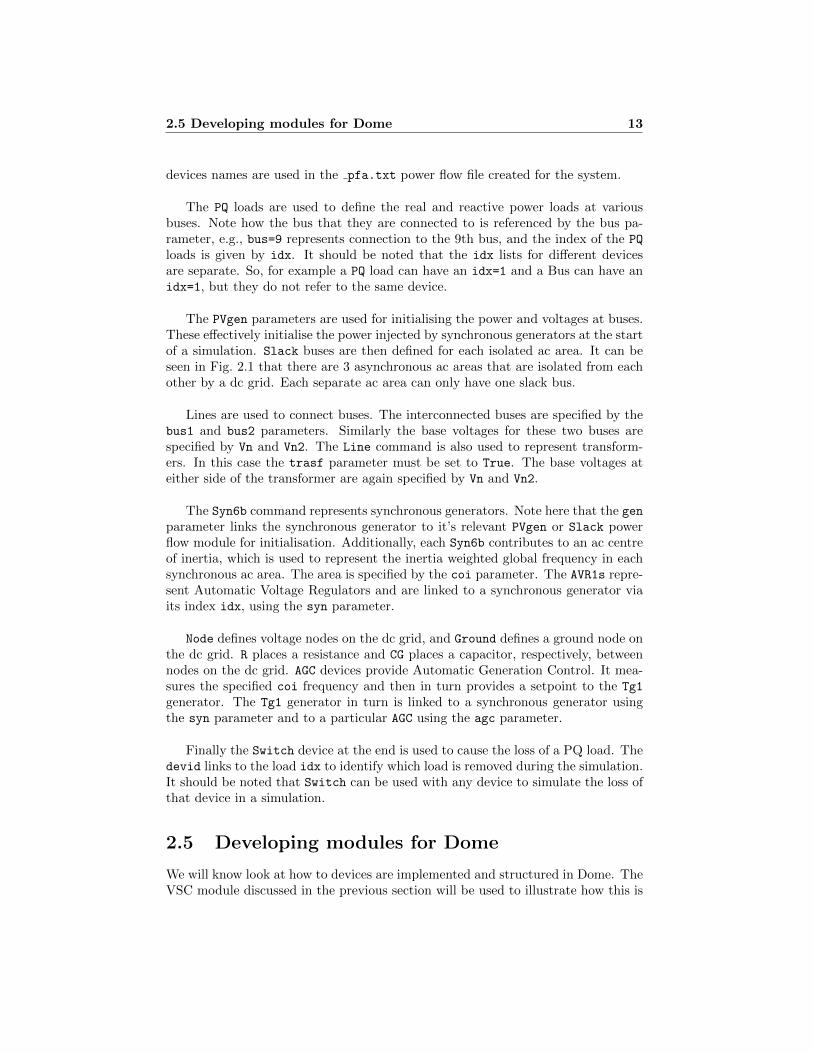
2.5 Developing modules for Dome 13
devices names are used in the pfa.txt power flow file created for the system.
The PQ loads are used to define the real and reactive power loads at variousbuses. Note how the bus that they are connected to is referenced by the bus pa-rameter, e.g., bus=9 represents connection to the 9th bus, and the index of the PQ
loads is given by idx. It should be noted that the idx lists for different devicesare separate. So, for example a PQ load can have an idx=1 and a Bus can have anidx=1, but they do not refer to the same device.
The PVgen parameters are used for initialising the power and voltages at buses.These effectively initialise the power injected by synchronous generators at the startof a simulation. Slack buses are then defined for each isolated ac area. It can beseen in Fig. 2.1 that there are 3 asynchronous ac areas that are isolated from eachother by a dc grid. Each separate ac area can only have one slack bus.
Lines are used to connect buses. The interconnected buses are specified by thebus1 and bus2 parameters. Similarly the base voltages for these two buses arespecified by Vn and Vn2. The Line command is also used to represent transform-ers. In this case the trasf parameter must be set to True. The base voltages ateither side of the transformer are again specified by Vn and Vn2.
The Syn6b command represents synchronous generators. Note here that the genparameter links the synchronous generator to it’s relevant PVgen or Slack powerflow module for initialisation. Additionally, each Syn6b contributes to an ac centreof inertia, which is used to represent the inertia weighted global frequency in eachsynchronous ac area. The area is specified by the coi parameter. The AVR1s repre-sent Automatic Voltage Regulators and are linked to a synchronous generator viaits index idx, using the syn parameter.
Node defines voltage nodes on the dc grid, and Ground defines a ground node onthe dc grid. R places a resistance and CG places a capacitor, respectively, betweennodes on the dc grid. AGC devices provide Automatic Generation Control. It mea-sures the specified coi frequency and then in turn provides a setpoint to the Tg1
generator. The Tg1 generator in turn is linked to a synchronous generator usingthe syn parameter and to a particular AGC using the agc parameter.
Finally the Switch device at the end is used to cause the loss of a PQ load. Thedevid links to the load idx to identify which load is removed during the simulation.It should be noted that Switch can be used with any device to simulate the loss ofthat device in a simulation.
2.5 Developing modules for Dome
We will know look at how to devices are implemented and structured in Dome. TheVSC module discussed in the previous section will be used to illustrate how this is

14 2 Tutorial
done. For those learning Python for the first time, there is extensive online helpfor Python. A good starting point is the following:
https://en.wikibooks.org/wiki/A_Beginner’s_Python_Tutorial
We will first discuss how Dome simulations work.
2.5.1 Internal Dome simulation
Dome simulations are based on the use of semi-implicit Differential Algebraic Equa-tions (DAEs). The typical implicit DAE is framed as follows:
x = f(x,y)
0 = g(x,y) ,(2.1)
where x are the system state variables and y are system’s algebraic variables, andf and g are functions of these variables. This form of representation, however, canlead to inefficiencies in simulation. For example, firstly equations usually have to berearranged so that the x variables are isolated on one side. Then if it is desired toset the time constant for an x variable to zero such that it becomes algebraic (thisis done if the dynamics of a particular variable in x are very fast in comparisonto the rest of the variables. By making it algebraic the whole simulation can besped up), it is necessary to construct a series of if/or statements which adds to theoverall simulation time.
Instead Dome uses a semi-implicit DAE representation as follows:[T x 0Rx 0
] [x0
]=
[f(x,y)g(x,y)
], (2.2)
which allows time constants to be zeroed in a straightforward fashion and reducesthe need to use additional intermediate states in certain DAE expressions. Notethat (2.1) is a special case of (2.2), where T x = In and Rx = 0. Note also thatthe form (2.1) can be always deduced from (2.2).
Power flow, small-signal stability and time domain analyses require the Jacobianmatrices of (2.2). Linearizations of f and g about the current operating point leadsto: [
T x 0Rx 0
] [∆x0
]=
[fx fy
gx gy
] [∆x∆y
], (2.3)
where fx, fy, gx, and gy are the sought Jacobian matrices.
For each model, the user has to provide the analytical expressions of equationsf and g; Jacobian matrices fx, fy, gx, and gy; and the time-constant matricesT x and Rx associated with the x.4
4Note that Tx and Rx do not need to be time-invariant. They are allowed to depend on both

2.5 Developing modules for Dome 15
2.5.2 Looking inside Python modules
We will now see how equations are entered into Dome’s Python classes in orderto develop dynamic state simulation modules. We will look at the Python fileconverter.py, given in Appendix C, and follow a few groups of equations to ex-amine their implementation. All the equations related to the VSC implementationare given in the paper “Generalized Model of VSC-based Energy Storage Systemsfor Transient Stability Analysis” by Alvaro Ortega and Federico Milano, publishedin the IEEE Transactions on Power Systems.
In the following we will work through the various pieces of code that define theDome modules. While there is a range of equations implemented in converter.py,we will focus on two simple equations first to illustrate how they are implemented.The first is the dynamic equation for it,d:
rtit,d + xtsit,d = xtit,q + vg,d − vt,d , (2.4)
where s represents the time derivative of a variable in the Laplace domain. Thesecond is the algebraic equation related to the terminal ac currents:
i2t,d + i2t,q = i2ac . (2.5)
Once we show how these equations are implemented we will then look at the morecomplex case of the PLL loop.
The class that implements the VSC shunt command in Dome is vsc shunt. Thisinherits the sub-class link which is also defined in converter.py and the sub-classdevice which is imported from the internal Dome functionality at the top of thefile:
class vsc_shunt(link, device):
Note that functionality must be imported using the from and import commands atthe top of the file. The command from determines where a command is importedfrom and import imports that particular piece of functionality. If altering a pieceof code that has been already developed internally in Dome the from statementmay use ... to reference the place from where the functions are taken. Files usedinternally in the Dome build folder on a Dome server, such as psat.ucd.ie, canuse ...device:
from ...device import core, device
Classes used to define devices in Dome are broken up into the following methods:
x and y, hence:
Tx = Tx(x,y)
Rx = Rx(x,y) .
However, Tx and Rx cannot implicitly depend on x, hence the notation semi-implicit for (2.2).Refer to Subsection 17.5.1 for more details on time-variant matrices Tx and Rx.

16 2 Tutorial
• init is the first function called for initialisation of the device.
• xfirst initialises variable values for power flow.
• ecall defines and calls the dynamic and algebraic equations of the device.
• The cjacs, ejacs, and getidx functions define the constant jacobians, non-constant jacobians, and the positions of off-diagonal jacobians, respectively.
Initialisation
The init function, the class constructor function, is the first function calledwhen an instance of a class is created. Thus this is the first method called invsc dq shunt:
def __init__(self, system, name):
This is used to initialise the various dynamic and algebraic variables as well asdefining the parameters that the user enters into the function.
The first command in the init method, super, is a built-in Python functionthat is used to call functions that have been inherited from subclasses. The link
class does not have an init . This implies here that the init method isinherited from the class device:
super(vsc_shunt, self).__init__(system, name)
The method super() calls methods inherited from subclasses. It can potentiallybe used in a more complex fashion. Refer tohttp://sixty-north.com/blog/series/pythons-super-explained
for a more in-depth explanation, and some caveats as regards the use of super().
The function self.link init() is called which calls the self.link init()
function in the link class. Please note that the functionality described in the re-mainder of this subsection is found in self.link init().
The internal Dome variables type and category are used to place the VSCin the VSC type device grouping, and in the categories of Circuit, Transmission,PowerElectronics and Interface.
self._group = ‘VSC’
self._category = ‘Circuit’, ‘Transmission’, ‘PowerElectronics’, \
‘Interface’
These labels are useful for when Dome needs to search for certain groups of devicesand for the command line option -G, e.g., printing
[janeOrJimmy@psat freqchaud]$ dome man VSC

2.5 Developing modules for Dome 17
at the terminal outputs the VSC group of devices.
Then the state, algebraic, and parameter variables associated with the system aredefined. The following defines the dynamic state for variable itd:
self._state.set(‘itd’, r‘i_t_d’, \
‘direct component of the ac series current’, \
‘pu(kA)’, ‘L’)
The command self. state.set() declares itd as a dynamic state variable, spec-ifies that itd should be written as i t d when used with Latex functionality(e.g. for use in the legend when plotting), gives a brief description for help filesas to what this variable is, gives the measurement units for the quantity, and fi-nally gives the time constant associated with the derivative of the variable which isL in this case. If the time constant is not specified it is assumed that it is equal to 1.
The following declares iac as an algebraic variable:
self._algeb.set(‘iac’, r‘i_ac’, \
‘magnitude of the ac series connection current’, \
‘pu(kA)’)
The 4 parameters here are equivalent to the first 4 parameters used in the functionself. state.set, except they define an algebraic variable in this case.
The self. conn.set command is used to define connections into a device classfrom various grids. Here this defines some dc node connections.
self._conn.set(’node1’, ’1st dc node’, (’v1’, ), ’Node’, (’v’, ))
self._conn.set(’node2’, ’2nd dc node’, (’v2’, ), ’Node’, (’v’, ))
The self.set datum command defines what user defined parameters will beentered to the module via the .dm file.
self.set_datum(’rt’, 0.01, ’transformer resistance’, ’pu(Ohm)’)
The above defines the resistance parameter as rt, gives it a default value of 0.01if it’s not specified in the .dm file, provides a brief description of it, and specifiesits units.
The set list function groups lists of parameters together where the first ele-ment is the name of the list. For example, the auxiliary list,
self.set_list(’_auxiliary’,
’L’, ’ste’, ’cte’,
’gt’, ’bt’, ’therr’)
is used to define lists of variables that are defined in the rest of the script.
Finally, a properties dictionary is constructed to determine which of the variousfunction calls are to be run:

18 2 Tutorial
self.set_dict(’properties’,
ecall = True,
ejacs = True,
pflow = True,
xinit = True,
cjacs = True)
Initial Guess for the Power Flow Analysis
Since the device is included in the power flow analysis (the properties pflow andxinit above are defined as True), it is necessary to provide an initial guess forthe variables defined in the device itself.5 The default variable initial guess is zero.Returning to the vsc dq shunt class definition, initialisation is conducted by thexfirst function. It in turn calls the self.link xfirst function inherited fromthe link sub-class.
While each command in self.link xfirst is not explicitly explained here,it is sufficient to understand how the variables are initialised using the followingcommands. Note that a variable or parameter, called var for example, that has beenbeen defined previously in self. init , is accessible using self.var. Functionssuch as div and mul perform element-wise matrix multiplication and division. Themassign function is used to assign values to state and algebraic variables:
massign(dae.y, 0.01, self.iac, self.u)
massign(dae.x, 0.01, self.itd, self.u)
Here self.iac and self.itd refer to the positions of iac and itd in dae.y anddae.x, respectively, where dae.y is the vector of all algebraic variables and dae.x
is the vector of all state variables.
Differential and Algebraic Equations
The function ecall is the first used for updating state and algebraic variables.
def ecall(self, dae):
The vsc dq shunt class’ ecall function first calls the inherited link class’ ecallfunction self.link ecall(dae). At the start of self.link ecall(dae), a num-ber of pointers to variables are created for convenience. The iac and itd pointersare given as follows:
iac = dae.y[self.iac]
itd = dae.x[self.itd]
5If the property pflow is False, then the device is initialised after the solution of the powerflow analysis. In this case, the initialisation is done in such a way that all the equations f and gdefined by the device are equal to zero at the power flow solution. The function where such aninitialisation is defined is called setx0.

2.5 Developing modules for Dome 19
It should be noted that self.iac and self.itd refer to the positions of iac anditd in dae.y and dae.x, respectively. In order to access the values of these vari-ables from the simulation, they are called as they appear in the code above, usingthe dae.y and dae.x vectors.
Defining algebraic equations is straightforward. The current balancing equationis represented in its 0 = g(x,y) form:
0 = i2t,d + i2t,q − i2ac . (2.6)
Equation (2.6) is implemented in self.link ecall(dae) using the following com-mand:
mupdate(dae.g, itd**2 + itq**2 - iac**2, self.iac, self.u)
The first argument says that this is an algebraic equation belonging to dae.g. Thesecond represents this equation written as 0 = g(x,y). The third argument stateswhich algebraic variable is updated using this equation. The final self.u argumentis used to determine whether the update is enabled or not.6
Differential equations are represented internally as T xx = f(x,y). In ecall,only the right-hand side has to be defined, i.e., f(x,y). The complete differentialequation that defines the dynamic of it,d is:
L it,d = rtit,d − xtit,q + vt,d − vg,d . (2.7)
In self.link ecall(dae), (2.7) is represented by:
mupdate(dae.f, mnmul(self.rt, itd, self.xt, itq) + vtd - vgd, \
self.itd, self.u)
The first argument says that this is a differential equation belonging to dae.f.The second represents this equation written as f(x,y). The third argument stateswhich dynamic variable is updated using this equation. The final argument is usedto determine whether the update is enabled or not. Note that the function mnmul
is a function of the Dome extension extras that defines the element-wise operationab− cd on arrays a, b, c and d.
Note that the L which is multiplied by it,d on the left-hand side of the equationwas defined as the last parameter used in the definition of it,d. This is repeatedhere for convenience:
self._state.set(‘itd’, r‘i_t_d’, \
‘direct component of the ac series current’, \
‘pu(kA)’, ‘L’)
When this final parameter is not explicitly defined it is given the default value of1.
6The attribute self.u is a vector of zeros and ones. If an element of self.u is equal to 1, thecorrespondent device element is active and/or connected to the grid. If an element of self.u isequal to 0, the correspondent device element is inactive and/or disconnected from the grid.

20 2 Tutorial
Jacobian Matrices
It is then necessary for simulations to define the Jacobian matrices fx, fy, gx,and gy. Three functions are needed for this task: getidx, cjacs, and ejacs, asdiscussed below.
The index of each of the positions of the derivatives is recorded in the getidx
functions. The vsc dq shunt class’ getidx method starts by calling the inheritedself.link getidx(dae) method from the link class. The existence of derivativesin fx and fy related to variables itd, itq, and xp are specified as follows:
dae.ifx += self.itd + self.itq + self.xp
dae.jfx += self.itq + self.itd + self.thetap
dae.ify += 2 * (self.itd + self.itq) + self.xp
dae.jfy += self.vgd + self.vgq + self.vtd + self.vtq + self.theta
Note that all elements above are Python lists, hence, the operator + indicatesconcatenation not addition. The positions of extra derivatives are given related toother equations in the system. The first two lines register that there are derivativesof the right-hand sides of the differential equations of itd, itq and xp with respectto itq, itd, and thetap, respectively. The dae.ifx and dae.jfx denote that theseare the positions in for fx derivatives. Similarly the dae.ify and dae.jfy linesdenote that the derivatives are from fy. Finally the 2 * (self.itd + self.itq)
is a compact way of writing self.itd + self.itq + self.itd + self.itq.
Note also that one does not need to define the positions of an index with respectto itself. For example, the following code:
dae.ifx += self.itd
dae.jfx += self.itd
is allowed but not necessary as diagonal elements of the Jacobian matrices fx andgy are always automatically included by Dome. On the other hand, since fy andgx are off-diagonal matrices, all their elements have to be defined explicitly.
The definition of Jacobian matrices are broken up into a number of sections.Constant elements of Jacobian matrices are registered in the cjacs function. Non-constant Jacobian matrix elements are placed in the ejacs function. Finally, theindex of the positions of non-zero derivatives with relation to variables in x and yare logged in the getidx function of the vsc shunt class definition. In turn, thevsc dq shunt class function calls the cjacs, ejacs, and getidx methods inheritedfrom the link class, namely link cjacs, link ejacs, and link getidx, respec-tively.
For itd, all derivatives are constant and so these are logged in the link cjacs
function. The following lines define the derivatives related to itd. For illustrationpurposes, it will demonstrated how the dae.ifx, dae.jfx, dae.ify, and dae.jfy

2.5 Developing modules for Dome 21
are constructed as these equations are defined:
Firstly the derivative of itd with respect to itself is specified:
sdupdate(dae.Fxc, self.rt, self.itd, self.u, -1)
No entry is specified yet for dae.ifx or dae.ify as this is the derivative of itd
with relation to itself.
Before outlining how the rest of the derivatives are specified, the sdupdate func-tion is explained. The first parameter represents the part of the Jacobian matrixto which the derivative belongs. The first letter after dae will be F or G to denotethat this is the derivative of a dynamic or algebraic equation, respectively. Thenext will be x or y to say that the derivatives are taken with respect to a dynamicor algebraic variable. Thus:
fx ⇒ dae.Fx fy ⇒ dae.Fy
gx ⇒ dae.Gx gy ⇒ dae.Gy
The c in this case is used to denote that the derivative is a constant. The secondparameter is the constant derivative of itd with respect the right hand side of (2.7).It is only necessary to specify itd this time as the derivative of the equation for itdis being derived with respect to itd itself. For the remaining derivatives relatedto (2.7) (spupdate), the derivative is taken with respect to another variable andso these are specified as will be seen in the coming paragraphs, e.g., the derivativeof the right-hand side of (2.7) with respect to it,q. The last argument, -1 in thiscase, is used to define the value that has to be used for the derivative for every zeroelement of self.u.7 Finally, self.u is used for enabling or disabling this derivative.
Hot Tip – One does not have to define the elements that multiplies the timederivatives of it,d (e.g., L) because this is automatically enabled in the definitionof the state variable (see the description above on the function self. state.set).
Hot Tip – The functions sdupdate and spupdate add the second argument tothe diagonal or off-diagonal elements, respectively, of the Jacobian matrices. Thefunctions sdassign and spassign substitute the diagonal or off-diagonal elements,respectively, of the Jacobian matrices with the given second argument. A similardifference is for mupdate and massign, which work on dense matrices (more oftenthan not, one-dimensional arrays). Note that, in the vast majority of cases, it ispreferable to use mupdate, sdupdate and spupdate than the correspondent assignversions. This prevents accidentally removing elements of arrays and Jacobian ma-trices defined by different devices.
Hot Tip – Any array of zeros and ones can be used to enable/disable a specificequation and Jacobian matrix element. self.u is the conventional name to acti-vate/deactivate a device. Other Boolean variables, generally starting with z (e.g.,
7This is necessary only for diagonal elements to avoid introducing singularities in the Jacobianmatrices fx and gy .

22 2 Tutorial
self.ze) are conventionally used to implement hard limits.
We now proceed in building the Jacobian matrices. The derivative of the dynamicfunction of itd with relation to itq is specified as follows:
spupdate(dae.Fxc, -self.xt, self.itd, self.itq, self.u)
Note that the format is similar to the previous sdupdate, except that the extravariable self.itq is specified after self.itd to show that this is the derivative ofitd with respect to itq.
The dynamic function belongs to f, and itq is a dynamic variable belonging to x.Thus an entry is made to dae.ifx and dae.jfx:
cat(dae.ifx, self.itd)
cat(dae.jfx, self.itq)
The derivative of the dynamic function of itd with relation to algebraic variablevtd is specified as follows:
spupdate(dae.Fyc, 1, self.itd, self.vtd, self.u)
The dynamic function belongs to f, and vtd is an algebraic variable belonging toy. Thus an entry is made to dae.ify and dae.jfy:
cat(dae.ify, self.itd)
cat(dae.jfy, self.vtd)
The derivative of the dynamic function of itd with relation to algebraic variablevgd is specified as follows:
spupdate(dae.Fyc, -1, self.itd, self.vgd, self.u)
The dynamic function belongs to f, and vgd is an algebraic variable belonging toy. Thus an entry is added to dae.ify and dae.jfy:
cat(dae.ify, self.itd, self.itd)
cat(dae.jfy, self.vtd, self.vgd)
A similar approach is used to represent non-constant derivatives, which aredefined using the ejacs function. The ejacs function of the class vsc dq shunt
calls self.link ejacs, which in turn contains the following 3 lines related to (2.6):
sdupdate(dae.Gy,-2*iac, self.iac, self.u, -1)
spupdate(dae.Gx, 2*itd, self.iac, self.itd, self.u)
spupdate(dae.Gx, 2*itq, self.iac, self.itq, self.u)
As described previously for the dynamic equations in cjacs the first parameterin sdupdate here represents that this is the derivative of an algebraic equationG with respect to y and x, for the dae.Gy and dae.Gx entries, respectively. The

2.5 Developing modules for Dome 23
first sdupdate represents the derivative of self.iac with respect to itself, whichis -2*iac. The next two represent the derivatives of the right-hand side of theequation iac with respect to itd and itq. Note that unlike in the cjacs casesthere is no c after the dae.Gy or dae.Gx parameters. This is because the deriva-tives are not constants, and vary with the current itd and itq measurements. Theself.u’s again here determine whether these variables are active in the code or not.
The getidx for the last 2 lines of code related to off-diagonal jacobian entriesare given as follows:
cat(dae.igx, self.iac, self.iac)
cat(dae.jgx, self.itd, self.itq)
Once all jacobians have been defined the indices of the off-diagonal elements areregistered in the getidx function as follows (via link getidx):
cat(dae.igx, self.iac, self.iac, self.p, self.p, self.q, self.q, \
self.vgd, self.vgq)
cat(dae.jgx, self.itd, self.itq, self.itd, self.itq, self.itd, self.itq, \
self.thetap, self.thetap)
The dae.igx and dae.jgx are used to store indices related to columns and rows inthe Jacobian that contain the relevant derivatives.
2.5.3 Defining the PLL equations
In the previous subsection the Python implementation of some straightforwardDome equation examples were provided. We will now examine the implementationof a PLL. This takes advantage of the semi-implicit representation of the system.Additionally this is a slightly more complex example, and it is hoped that this willillustrate that by rearranging the transfer functions a highly efficient implementa-tion of the equations is possible.
The following is the typical diagram that is given for a PLL:
Kpd
1+sT1p
sT2p
Kvcos
θerr θpθ+
−
By rearranging the diagram into the following, a simple implementation of the PLLis possible in Dome, which needs only one extra variable for implementation, xp:
Kpd
sT2p
Kvco(1+sT1p)
s
θpθxp+
−

24 2 Tutorial
The equations governing the PLL are now given by:
T2psxp = Kpd(θ − θp)
sθp −KvcoT1psxp = Kvcoxp .(2.8)
In link init the following define thetap and xp as state variables
self._state.set(‘thetap’, r‘\theta_p’, \
‘PLL voltage phasor angle’, ‘rad’)
self._state.set(‘xp’, r‘x_p’, \
‘state variable of the PLL filter’, \
‘-’, ‘T2p’)
It is at this stage that the time constants, 1 and T2p, are associated with thetap
and xp, respectively (the default time constant of 1 for thetap denotes a pure in-tegrator).
The function ecall considers the updates to xp and thetap when the derivativeson the left hand side of the equations are set to 0.
mupdate(dae.f, mul(self.Kpd, self.therr), \
self.xp, self.u)
mupdate(dae.f, mul(self.Kvco, dae.x[self.xp]), \
self.thetap, self.u)
Finally, the derivatives of the equations are given in cjacs
sdupdate(dae.Fxc, 0, self.xp, self.u, -1)
spassign(dae.Tx, -mul(self.Kvco, self.T1p), self.thetap, \
self.xp, self.u)
spupdate(dae.Fyc, self.Kpd, self.xp, self.theta, self.u)
spupdate(dae.Fxc,-self.Kpd, self.xp, self.thetap, self.u)
sdupdate(dae.Fxc, 0, self.thetap, self.u, -1)
spupdate(dae.Fxc, self.Kvco, self.thetap, self.xp, self.u)
For the fx derivatives the techniques outlined previously are used in the above.However, in the example of the PLL another derivative is used in the updating ofthetap. This coefficient must be placed in a off-diagonal position in the T x matrix,denoted by dae.Tx here. Note that spassign is used here to allocate this variable.The coefficient −KvcoT1p on the left hand side of the relevant equation, associatedwith sxp is entered in the relevant off-diagonal entry in the T x matrix.
Now that a number of examples have been given why not try follow the construc-tion of some of the other equations in the paper “Generalized Model of VSC-basedEnergy Storage Systems for Transient Stability Analysis” to try and see if you canfollow how each equation has been executed in converter.py.

Chapter 3
Command Line Options
Once the installation is complete, two commands are available: dome that allowssolving simulations.
As any Unix-like command both dome provides a variety of command line op-tions that allow adjusting the behaviour to user’s needs. This chapter describes indetails all command line options.
3.1 Generalities
The general dome syntax is as follows:
$ dome command [[command2] [--opt name1=opt value]
[--opt name2] ...] [data file name]
where, following the usual Unix notation, square brackets indicates optional syntax.The command line accepts any number of options. However, some options interruptthe execution of the program (e.g., --help) and hence make following options idle.
Available values for command can be obtained by typing:
$ dome --help
or
$ dome -h
which returns:
usage: dome [-h] command [options] ...
Dome is a software tool for power system modelling and simulation
optional arguments:
-h, --help show this help message and exit
25

26 3 Command Line Options
valid commands:
command [options]
core core functions and routines (default)
man query device and setting formats
plot plot simulation results
stat distributions and statistics
convert convert data files
sync synchronize with server repositories
install install external libraries
test run tests for extensions
grid create synthetic network
tree browse device tree
ver print version
warranty print warranty
wipe wipe output files
The command core can be omitted, except for printing the help message above.To get a list of the commands and/or options for each main commands, type,
for example:
$ dome convert -h
which returns:
usage: dome convert [-h] [-p PATH] [-o OUTPUT_FORMAT] [-i INPUT_FORMAT]
[-s SETTINGS] [-a ADDFILE]
[datafile [datafile ...]]
positional arguments:
datafile input data file
optional arguments:
-h, --help show this help message and exit
-p PATH, --path PATH path of the data file
-o OUTPUT_FORMAT, --output_format OUTPUT_FORMAT
name of output file format, see <dome man parsers>
-i INPUT_FORMAT, --input_format INPUT_FORMAT
name of input file format, see <dome man parsers>
-s SETTINGS, --settings SETTINGS
file name for custom settings
-a ADDFILE, --addfile ADDFILE
additional data file needed by some formats
3.2 dome core Options
This section describes exclusively the options of the command core, which runspower flow analysis and other numerical analysis. All options can be printed usingthe command:
3.2 dome core Options 27
dome core -h
Note that, since core is the most commonly used command, it can be omitted inthe calls. So, for example, the command:
dome core -r tds datafile.dm
is equivalent to:
dome -r tds datafile.dm
and both commands solve the power flow and then the time domain simulation ofthe file datafile.dm.
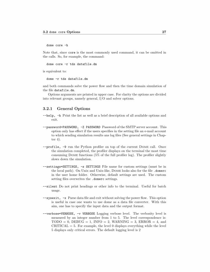
Options arguments are printed in upper case. For clarity the options are dividedinto relevant groups, namely general, I/O and solver options.
3.2.1 General Options
--help, -h Print the list as well as a brief description of all available options andexit.
--password=PASSWORD, -Z PASSWORD Password of the SMTP server account. Thisoption only has effect if the users specifies in the setting file an e-mail accountto which sending simulation results ans log files (See general settings in Chap-ter 4).
--profile, -9 run the Python profiler on top of the current Dome call. Oncethe simulation completed, the profiler displays on the terminal the most timeconsuming Dome functions (5% of the full profiler log). The profiler slightlyslows down the simulation.
--settings=SETTINGS, -s SETTINGS File name for custom settings (must be inthe local path). On Unix and Unix-like, Dome looks also for the file .domercin the user home folder. Otherwise, default settings are used. The customsetting files overwrites the .domerc settings.
--silent Do not print headings or other info to the terminal. Useful for batchusage.
--sysexit, -x Parse data file and exit without solving the power flow. This optionis useful in case one wants to use dome as a data file converter. With thisaim, one has to specify the input data and the output format.
--verbose=VERBOSE, -v VERBOSE Logging verbose level. The verbosity level ismeasured by an integer number from 1 to 5. The level correspondence is:TODO = 0, DEBUG = 1, INFO = 2, WARNING = 3, ERROR = 4, andCRITICAL = 5. For example, the level 0 displays everything while the level5 displays only critical errors. The default logging level is 2
28 3 Command Line Options
3.2.2 IO Options
--addfile=ADDFILE, -a ADDFILE Additional data file needed by some formats(see also Chapter 5).
--dae, -D Write a brief summary of DAE statistics of the input data file.
--drawing, -m plot map of power flow results. This option has an effect onlyif the input data includes topological information or if used in conjunctionwith option --gis (see above). See the settings Plot for details on customiz-able options. Available types are: congestion, graphtool, networkx, andtemperature.
--dump=DUMP, -d DUMP Specify the name of the output file to which simulationresults are dumped.
--gis=GIS, -J GIS GIS file (JML format). This file specifies through an XMLscheme, topological information (see also Chapter 5).
--input=INPUT FORMAT, -i INPUT FORMAT Format of the input data file. Ac-cepted formats are: card, cepel, cfins, chapman, cim, cyme, digsilent,dome, epri, eurostag, flowdemo, fluprog, ge, gridcal, gridlabd, hdf,ieee, inptc1, interpss, ipsapower, ipssdat, jml, m3, matpower, minpower,netlist, odm,opendss, pcflo, pickle, pndm, powerworld, psap, psat, psse,pst, pypower, reds, sepe, settings, simpow, simulink, solution, tsinghua,ucte, ukgds, vst, webflow, wood, and xml. See also Chapter 5. Observe thatspecifying the input format is not mandatory. If no format is specified, Domeattempts to recognize the input data format using heuristic rules. However,to avoid issues and save time, it is recommended to specify the input dataformat.
--input wrapper=FILENAME, -$ Custom input data wrapper (the file must belocated in the local data path).
--log=LOG, -l LOG Explicitly assign a name for the output log file. By default,dome log file.out is used.
--no output, -n Force not to write any output file. This may help save sometime in case of large simulations.
--output=OUTPUT, -O OUTPUT Custom output file name. The default is the sameinput data file name with an adequate suffix and extension. The extensiondepnds on the output format selceted by the user. By default, the outputformat is a plain ASCII text (extension .txt).
--output format=OUTPUT FORMAT, -o OUTPUT FORMAT Format of the output datafile. Accepted formats are: card, dome, gams, gamsfull, hdf, ieee, jacs,latex, layout, lookup, meshed, pickle, psat, radial, sepe, solution,sostools, and xml. See also Chapter 5.

3.2 dome core Options 29
--output wrapper=FILENAME, -% Custom output data wrapper (the file must belocated in the local data path).
--overwrite, -z Overwrite logging and report files. By default, output files areassigned conventional names and overwritten at each execution of Dome.
--path=PATH, -p PATH Path to the input data file. It can be a relative or anabsolute path.
--summary, -Y Write a brief summary of the data file. The data file is parsedand relvant information about devices included in the file is printed out.This option can be used in conjunction with option --exit if the power lfowanalysis is not required.
3.2.3 Solver Options
--checkjacs, -j Check analytical Jacobian matrices using numerical differentia-tion. This option is useful when developing new devices. Of course, this op-tions does not state whether the device equations are consistent, just checkswhether the analytical Jacobian elements coincides with the numerical dif-ferentiation of device equations. Hence, this option allows checking if theanalytical Jacobian corresponds to the device equations. Observe that thenumerical differentiation fails whenever a hard limit is binding.
--force, -F Force continuing the execution even if the power flow routine doesnot converge. By default, is the power flow has convergence issues, Domeexit with an error message. However, during the development of new devices,it may be useful to check analytical Jacobian matrix elements since these areoften the cause of the convergence failure (see option --checkjacs above).With this aim, it may be useful to reduce the maximum number of powerflow iterations to 1 or 2. In fact, when the power flow does not converge,variable values often increase more than quadratically and even get the not-a-number (NaN) value. The numerical differentiation is more informative ifvariable values are close to nominal ones.
--ncpus=N, -M N Run N parallel processes using the input file list. If only one fileis given, then N simulation are run in parallel using the same input data file.With one input file, this option is particularly useful when solving probabilis-tic and stochastic analyses. For example:
$ dome -M 100 -r TDS ieee14.dm
will solve 100 time domain simulations of the file ieee14.dm. Solutions willbe numbered from 0001 to 0100, e.g.:
ieee14_job0001_pfa.txt
ieee14_job0001.out
ieee14_job0001.dat

30 3 Command Line Options
ieee14_job0001.lst
ieee14_job0002_pfa.txt
ieee14_job0002.out
ieee14_job0002.dat
ieee14_job0002.lst
...
...
ieee14_job0100_pfa.txt
ieee14_job0100.out
ieee14_job0100.dat
ieee14_job0100.lst
It is also possible to run in parallel simulations of different files. For example:
$ dome -M 2 -r TDS ieee14.dm newengland.dm
In this case, output files will have usual names:
ieee14_pfa.txt
ieee14.out
ieee14.dat
ieee14.lst
newengland_pfa.txt
newengland.out
newengland.dat
newengland.lst
--idlecpus If the number of CPUs available on the server is m, idlecpus is setto p, and ncpus is set to n, run the n processes in clusters of minm−p, 1 ata time. This option is recommended to prevent locking the server when boththe number of parallel processes n and the CPU time required to completeeach process are high. This option is used along with option --ncpus N. Forexample:
$ dome -M 100 --idlecpus 2 -r TDS ieee14.dm
will solve 100 time domain simulations of the file ieee14.dm always leavingat least 2 idle CPUs on the server.
--onlyjacs, -0 Check analytical Jacobian matrices using numerical differentia-tion. This option is similar to checkjacs but does not attempt to solve thepower flow analysis. This option can be useful during the debugging phase ofa new device model in case the Jacobian matrix is singular.
--routine=ROUTINE, -r ROUTINE Set the routine to be solved after power flowanalysis. Available solvers are:
3.3 Examples 31
ACS admission control strategy (for electric vehicles);
CPF continuation power flow analysis;
EIG eigenvalue analysis;
EQV network equivalents;
GRA graphic and topological network analysis;
OPF optimal power flow analysis;
SCA short-circuit analysis;
SE state estimation
TDS time domain integration.
Abbreviations C, E, O and T are and lower cases are also recognized. Only onesolver per run is allowed. Although each solver performs some basic controlover the input data, the user should always do a careful check of the datafile to be sure that these are conssitent with the solver. The user should alsocarefully study the default values assumed by the solvers in case no explicitsetting is provided. Solver settings are detalied in Chapter 4.
3.3 Examples
Running the power flow with implicit format assumption:
$ dome foo.txt
Running the power flow with explicit format specification:
$ dome -i ieee foo.txt
Running the power flow using a relative path:
$ dome -p foopath1/foopath2 foo.txt
Runnig the power flow using an absolute path:
$ dome -p "/home/user name/foopath" foo.txt
Solving a time domain simulation:
$ dome -r TDS foo.txt
Solving the CPF analysis and check the consistency of analytical Jacobian matrices:
$ dome -r CPF -j foo.txt
Forcing the check of the consistency of analytical Jacobian matrices in case thepower flow analysis does not converge:
$ dome -j --force foo.txt

32 3 Command Line Options
Converting a file in IEEE CDF into Dome format without solving the power flow:1
$ dome -i ieee -o dome -x foo.txt
Getting the summary of a data file without solving the power flow:
$ dome --summary -x foo.txt
Looking for help on the device Line:
$ dome man Line
Looking for all devices whose name starts with T:
$ dome man search T
Looking for all devices whose name contains the token Line:
$ dome man search "\w*Line"
Printing all options of the settings for CPF analysis:
$ dome man CPF
1Forcing Dome to exit before solving the power flow can be inconsistent if the parser requiresthe power flow solution to create the output file.

Chapter 4
Settings
4.1 Available Settings
The behavior of Dome and of each solver can be adjusted through a set of settings.Dome assigns default values to all settings. Such default values can be customizedin several ways, as explained in the following subsection.
Settings are divided into groups. Each group can include subgroups. Groupsand subgroups as well as a short description of each option of each group can beretrieved using the command:
$ dome -A All
Currently defined setting groups are: Settings, Plot, PF, TDS, CPF, OPF, SSSA,SCA, ACS, EQUIV, SOS, SMTP, Plot, and Graph. Each group includes a set of options.All options displayed using the previous command can be customized by the user.One can also query the options of a single group:
$ dome -A PF
which should provide an output similar to the following:
Class <PF>
Settings for power flow analysis
---------------------------------------------------------------------------
Parameter | Description | Default
---------------------------------------------------------------------------
flatstart | use flat start for solving power flow | False
| analysis |
inpvpq | iteration number at which PV-PQ | 2
| switching begins (for power flow |
| analysis) |
maxit | maximum number of iteration of the | 20
| power flow analysis |
33

34 4 Settings
pv2pq | switch PV to PQ in case of reactive | False
| power limit violation during power |
| flow analysis |
report | power flow report type. Alternatives: | default
| [default, extended] |
show | show iteration status during power | True
| flow analysis |
solver | power flow solver method. | NR
| Alternatives: |
| <NR>: standard Newton-Raphson |
| <XB>: fast decoupled power flow (XB) |
| <BX>: fast decoupled power flow (BX) |
| <DC>: dc power flow |
| <RK4>: Runge-Kutta’s order 4 formula |
| <RK6>: Runge-Kutta’s order 6 formula |
| <Braz>: robust Braz-Castro’s method |
| <Robust>: robust Newton-Raphson |
| <Gauss>: Gauss-Seidel’s method |
| <Jacobi>: Jacobi’s method |
| <Dishonest>: dishonest Newton-Raphson |
| <BFS>: back-forward sweep |
| <BFSCL>: parallel back-forward sweep |
| based on Nvidia GPU |
| <LM>: Levenberg-Marquardt method |
| <HEM>: Holomorphic embedded method |
sortbuses | criterion used to sort buses in power | data
| flow report. Alternatives: [id, name, |
| data, natural] |
static | discard dynamic devices that are | False
| initialized after power flow analysis |
switch1pv | switch only one PV to PV per | True
| iteration during power flow analysis |
switch2nr | allow switching to Newton-Raphson | False
| method if the power flow convergence |
| error is sufficiently small |
units | units used in the power flow report. | pu
| Alternatives: [pu, MVA, kVA, VA] |
usedegree | use degree instead of rad in power | False
| flow report |
violations | include limit violations in the power | False
| flow report |
---------------------------------------------------------------------------
Subclass <PF.LM>
Settings for the Levenberg-Marquardt method
---------------------------------------------------------------------------
Parameter | Description | Default
---------------------------------------------------------------------------

4.1 Available Settings 35
adaptive | if True, the step size is variable | True
| and adapted to equation mismatch |
mu | reference step size | 0.01
norm | norm type used to compute the | nrm2
| variable increment. Alternatives: |
| <nrm2>: Euclidean norm |
| <nrmoo>: infinity norm |
| <nrm22>: square of the Euclidean norm |
p0 | parameter for the adaptive step size | 0.0001
| (0 <= p0 <= p1) |
p1 | parameter for the adaptive step size | 0.25
| (p0 <= p1 <= p2) |
p2 | parameter for the adaptive step size | 0.75
| (p1 <= p2 <= 1) |
theta | parameter that weight the convex | 1.0
| combination of ||F|| and ||J^T*F|| |
---------------------------------------------------------------------------
Static report saved to file <setting_help.txt>
The following command produces the same output as the above:
$ dome -q PF
The user can also retrieve information on a single option of a certain group, forexample:
$ dome -B PF.solver
which should provide an output similar to the following:
--------------------------------------------------------------------
Help on setting parameter <PF.solver>:
Power flow solver method. Alternatives:
<NR>: standard Newton-Raphson
<XB>: fast decoupled power flow (XB)
<BX>: fast decoupled power flow (BX)
<DC>: dc power flow
<RK4>: Runge-Kutta’s order 4 formula
<RK6>: Runge-Kutta’s order 6 formula
<Braz>: robust Braz-Castro’s method
<Robust>: robust Newton-Raphson
<Gauss>: Gauss-Seidel’s method
<Jacobi>: Jacobi’s method
<Dishonest>: dishonest Newton-Raphson
<BFS>: back-forward sweep
<BFSCL>: parallel back-forward sweep based on Nvidia GPU
<LM>: Levenberg-Marquardt method
<HEM>: Holomorphic embedded method
The default value is <NR>
--------------------------------------------------------------------

36 4 Settings
Subgroup queries use the syntax group.subgroup. For example:
$ dome -A PF.LM
shows the options of the Levenberg-Marquardt method for power flow analysis, i.e.,only the options of the PF.LM subgroup (see output of the command dome -A PF
above). Similarly, specific options of subgroups can be queried using the syntaxgroup.subgroup.option. For example:
$ dome -B Graph.SM.distr
shows the available distributions for the generation of random meshed grid basedon the small-world topology.
4.2 Customizing DOME Behavior
There are currently five ways to customize Dome behavior:1
1. Place a file called .domerc in the user home folder.2 Dome recognizes the file.domerc only on Unix-like systems. The use of the file .domerc is deprecatedin favor of the file config.ini (see next item).
2. Place a file called config.ini in the folder .dome or .config/dome withinthe user home folder. Dome recognizes the file config.ini only on Unix-likesystems. This method is equivalent to that based on the file .domerc.
3. Create a setting file in the current data folder and call it at execution timeusing the commnad option -s setting file.txt. If the extension of the fileis .ini, it is parsed assuming the syntax of the config.ini file,otherwise thesyntax of the file .domerc is assumed (see formats below).
4. Include as many instances of the meta-device Tuning within the data file. Re-fer to the on-line help of the meta-device for the syntax (i.e., use the commanddome -q Tuning).
5. Include in the data file device-like instances of the settings, as follows:
PF, solver=’XB’, flatstart=True
TDS, step=’fixed’, tstep=0.01
This approach is equivalent to the that based on the meta-device Tuning.
The methods above follow a hierarchical scheme, i.e., the instances of the meta-device Tuning overwrite custom settings of the local file setting file.txt, whichoverwrites common user settings defined in the file .domerc or config.ini. If
1Actually, there is a fifth way, which consists in changing default values in the Dome sourcecode. However, this approach can be used only by developers. Note that, to allow reproducibleresults, change of the default values of the source code should be avoided as much as possible.
2On Unix-like systems, a file preceeded by a dot is a hidden file.

4.2 Customizing DOME Behavior 37
both files .domerc or config.ini exist, config.ini overwrites settings defined in.domerc. It is recommended not to use .domerc or config.ini together.
The format of .domerc is inherited from typical Unix-command setting files.Each line assigns a value to one Dome variable. The syntax is as follows:
class name.attribute name = attribute value
where class name is one of the following groups:
CPF Continuation power flow settings.EQUIV Equivalencing procedure settings.PF Power flow settings.OPF Optimal power flow settings.Settings General settings.SMTP SMTP settings for sending Dome results by e-mail.SOS Polynomial (sum of squares) settings.SSSA Small-signal stability settings.TDS Time domain simulation settings.
The attribute value can be any number, a Python Boolean (i.e., True or False),None, or a string. Strings have to be included in ’ or ". Lines starting with # arecomments.
The following is an example of setting file.
Settings.freq = 60.0
Settings.distrsw = False
Settings.export = ’txt’
Settings.forcepq = False
Settings.library = ’SUPERLU’
Settings.coi = True
Settings.connectivity = True
Settings.pvdir = False
Settings.seed = False
# Power flow settings
PF.solver = ’NR’
PF.report = ’default’
PF.pv2pq = False
PF.violations = False
PF.maxit = 100
PF.sortbuses = ’data’
# Power flow Levenberg-Marquardt settings
PF.LM.adaptive = True
PF.LM.mu = 0.01
# Small-world topology settings
Graph.SM.ltc_k = 5
Graph.SM.mdeg = 4.5
Graph.SM.n0 = 100

38 4 Settings
Graph.SM.ck = 4
# Time domain integration settings
TDS.pq2z = True
TDS.tf = 30
TDS.resetangles = True
TDS.fixt = True
TDS.tstep = 0.01
# SMTP settings
SMTP.email = False
SMTP.server = ’smtp.mail.uclm.es’
SMTP.username = ’Federico.Milano’
SMTP.address = ’[email protected]’
SMTP.password = ’’
SMTP.port = 587
# Continuation power flow settings
# CPF.ending = ’all solutions’
CPF.method = ’perpendicular intersection’
CPF.single_slack = False
CPF.reactive_limits = False
CPF.nump = 100
CPF.mu_init = 1.0
CPF.step = 0.5
CPF.hopf = True
# Network equivalent settings
EQUIV.bus_selec = ’area’
EQUIV.area = 5
EQUIV.method = ’REI’
EQUIV.lossless = True
The syntax of the file config.ini is as follows: The syntax is as follows:
[class name]
attribute name = attribute value
Attributes and comments follow same rules as for the fiel .domerc. The followingis an example of config.ini file:
[Settings]
freq = 50.0
distrsw = False
export = ’txt’
forcepq = False
library = ’NICSLU2’
mva = 100
tol = 1e-5
[Graph.SM]

4.3 Permanently Adding Custom Devices 39
mdeg = 4.5
n0 = 100
ck = 4
[PF.LM]
adaptive = True
mu = 0.01
[PF]
solver = ’NR’
#report = ’default’
pv2pq = False
maxit = 20
#sortbuses = ’data’
flatstart = False
#usedegree = False
#units = ’pu’
#violations = True
inpvpq = 2
switch2nr = False
[TDS]
pq2z = False
tf = 30
resetangles = False
fixt = True
step = ’quantized’
tstep = 0.01
solver = "DH"
limits = True
#method = ’qss’
shrink = True
debug = False
The password for the SMTP can be included in the .domerc and config.ini files.Note, however, that the password will be not protected.
4.3 Permanently Adding Custom Devices
Dome allows extending the standard library of devices by loading local modules.There are currently two ways to import user-defined device, permanently and on-the-fly. The remainder of this section on discusses the former method. How toadd user-defined on-the-fly through the data file and local modules is discussed inSection 9.5 of Chapter 9.
To permanently add user-defined devices to Dome’s standard library, one hasto prepare a set of files and folders, as follows. First create the folder .dome inthe user’s home folder. Then crate within this folder a folder called devices and afile called init .py – this file can be empty. Then, place in the folder devices

40 4 Settings
the Python modules containing the user-defined devices and a file called againinit .py. The complete tree of the directories and files is shown in Fig. 4.1.
devices
__init__.py
config.ini
__init__.py
module1.py
module2.py
...
.dome
User home folder
Figure 4.1: Structure of the directory tree to permanently include user’s defineddevices to Dome standard library.
The content of the file init .py within folder .dome/devices must indicatethe modules and the devices to be added to Dome. The following script is anexample:
# local devices
__all__ = [’module1’, ’module2’, ]
__devices__ = ’module1’:
((’freqbus’, ’freqcoi’, ’freqdiv’, ),
(’WTFRbus’, ’WTFRcoi’, ’WTFRdiv’, ),
(’WindFreq’, ’WindFreq’, ’WindFreq’, )),
’module2’:
((’newavr1’, ’newavr2’, ’newavr3’, ),
(’NewAVR1’, ’NewAVR2’, ’NewAVR3’, ),
(’Avr1’, ’Avr1’, ’Avr1’, ))
The dictionary devices has as keys the names of the modules included in thefolder. The values of this dictionary are tuples with three items:
1. A tuple of the names of the classes included in the module that defines thedevices to be added to Dome.
2. A tuple of the names of the devices as to be instantiated in Dome. Thesenames are the ones that will be used in the data files to indicate these devices.
3. A tuple of the names of devices already included in Dome after which theuser-defined devices has to be added. It is a good idea to add the user-defined devices in the same locations as “similar” devices already included in

4.3 Permanently Adding Custom Devices 41
the Dome standard library to prevent initialization issues. The items of thistuple can be None. In this case, user-defined devices will be appended at theend of the Dome device list.
Note: The ability of defining local devices can foster the proliferation of severalvariants of existing devices with little but incompatible differences. To preventunexpected results, the permanent custom library should be utilised only to testnewly developed devices that, once completed, should be included in the mainDome distribution.


Chapter 5
Data Format
Dome accepts input data in several formats, including IEEE CDF, PSAT, PSS/Eand DigSILENT. The list of all accepted formats can be obtained with the com-mand1
$ dome man parsers
The output of such a command should look like the following:
Parsers of supported I/O data formats
Input Formats
-----------------------------------------------------------------
card cepel cfins chapman cim
cyme digsilent dome epri eurostag
flowdemo fluprog ge gridcal gridlabd
hdf ieee inptc1 interpss ipsapower
ipssdat jml m3 matpower minpower
netlist odm opendss pcflo pickle
pndm powerworld psap psat psse
pst pypower reds sepe settings
simpow simulink ucte solution tsinghua
ukgds vst webflow wood xml
Output Formats
-----------------------------------------------------------------
dome ieee latex psat sepe
card pickle radial layout hdf
xml meshed gams gamsfull sostools
Static report saved to file <dome parsers.txt>
1Some parsers are experimental and highly incomplete (e.g., Netlists and CIM).
43

44 5 Data Format
When launched with a data file as an argument, Dome tries some heuristics todetermine the format of the data. These heuristics are based mostly on the fileextensions and on parsing the first few lines of the files and look for keywordsspecific of the supported data formats. If such heuristics fail, the user can specifythe input data format using the option -i followed by the name of the parser, i.e.,one of the names of the first list above. For example:
$ dome -i psse datafile.raw
If the input file is split into more than one file, extra input files can be specifiedusing the -a option. For example:
$ dome -i psse datafile.raw -a datafile.dyr
5.1 Dome Format
The specifications of the internal Dome raw format as obtained by the command
$ dome -e
The output of such a commend is briefly outlines in the remainder of this chapter.
5.1.1 Header
The very first line of the data file must be:
# DOME format version 1.0
Optionally, adding another line that starts with the # sign will be assumed to be ashort description or title of the data file.
5.1.2 Device Data
Conventionally, the name of the component starts in the first column. Blank spacesbefore the names of the devices are allowed but not recommended.
Data follows in Property Name = Value pairs, separated by commas. For example:
Bus, Vn = 20.0, idx = 1, name = "Bus 01", voltage = 0.95
Note that data in form of strings must be delimited by "" or ’’. The special stringsTrue and False do not require quotes.
Data can span multiple lines:
Line, Vn = 230.0, Vn2 = 230.0, b = 0.04375, bus1 = 5, bus2 = 6,
idx = 1, imax = 1.0, name = "Line 5-6", r = 0.0025, x = 0.025

5.1 Dome Format 45
The lines following the first one should be indented. The last line of a device cannotend with a comma.
Data in form of arrays must be delimited by brackets []. Each element of the arraymust be separated by semicolons ;. For example:
Display, devName = "Line", devID = "Line 16",
xcoord = [7.725; 7.725; 8.250; 8.250],
ycoord = [4.875; 4.725; 4.650; 4.500]
Float data support simple operations (+, -, *, /). For example:
Line, Vn = 230.0, Vn2 = 230.0, b = 2*0.04375, bus1 = 5, bus2 = 6,
idx = 1, imax = 1.0, name = "Line 5-6", r = 0.0025/2,
x = 0.025+0.001
Scientific notation is supported for floating point data. This is obtained by addinga trailing letter to the number. For example:
Line, Vn = 0.230k, Vn2 = 0.23k, b = 43.75m, bus1 = 5, bus2 = 6,
idx = 1, imax = 1.0, name = "Line 5-6", r = 2.5m, x = 25m
Supported letters for the scientific notation are:
y z a f A p n u m c d da h k M G T P E Z Y
Dome provides an in-line help to show the parameters that can be defined foreach device. This is obtained with the command:
$ dome man DeviceName
For example, the command:
$ dome man Bus
should return something like the following:
Device <Bus>
- Type: Topology
- Categories: Transmission, Topology
ac bus (polar coordinates)
------------------------------------------------------------------------
Parameter | Description | Default | Units
--------------+--------------------------------+------------+-----------
# Sn | Power rate | 100.0 | MVA
* Vn | Voltage rate | 220.0 | kV
angle | Initial guess for the bus | 0.0 | rad
| phase angle | |
area | Area id | 1 | -

46 5 Data Format
# fn | Frequency rate | 60.0 | Hz
network | Network id | 1 | -
phase | Bus phase [a, b, c, 0, 1, 2] | 0 | -
region | Region id | 1 | -
u | Connection status | 1.0 | bool
vmax | Maximum voltage | 1.1 | pu(kV)
vmin | Minimum voltage | 0.9 | pu(kV)
voltage | Initial guess for the bus | 1.0 | pu(kV)
| voltage magnitude | |
------------------------------------------------------------------------
<Bus> is an instance of class <bus> from module
<dome.devices.topology.bus>
(*) Mandatory parameter.
(#) Non-zero parameter.
Static report saved to file <quick_help.txt>
It is not necessary to define all parameters of a given device. If a parameter isnot defined, the default value will be used. The data format specifies the parametersthat have to be defined. Such parameters are marked with an * in the list generatedwith the command man, as shown in the example above. Parameters can be providedin any order, but cannot be duplicated. For example the following will not work:
Device, param1 = val1, param1 = new val1
All Dome devices include three parameters that are not shown in the list gen-erated with the command man. These are:
• idx: the ID of the device. The ID must be unique for devices of the samekind (see also Chapter 8).
• name: the given name of the device. Names do not need to be unique fordevices of the same kind, but it is anyway recommended to assign uniquenames to easily identify the devices in the solution reports returned by Dome.
• u: the status of the device. 1 means that the device is enabled, on-line and/orconnected to the grid. 0 means that the device is disabled, inactive and/ordisconnected from the grid.
It is not mandatory to define idx, name or u. By default u = 1 and default valuesare assigned to idx and name. To specify the identification idx is only needed whenone wants to connect a device to another device, e.g., a load to a bus. IDs can beeither numbers or strings, as long as they are unique per each device kind.
The following is an example of correct usage of IDs:
Bus, Vn = 400.0, idx = 1, name = ’Bus1’
Bus, Vn = 400.0, idx = 2, name = ’Bus2’

5.2 Macros 47
Line, bus1 = 1, bus2 = 2, r = 0.1,
x = 0.2, b = 0.04
Slack, bus = 2, v0 = 1.0
PQ, bus = 1, p = 0.9, q = 0.6
5.1.3 Comments
Comments starts with a # in the first column:
# This is a single-line comment
Trailing comments are allowed:
Bus, idx = 1, Vn = 230 # This is a trailing comment
Comments spanning multiple lines starts with /* and ends with */. For example:
/*
Comments spanning
...
...
multiple lines
*/
5.2 Macros
The Dome format supports several useful macros. In particular, the macros ALTERand INCLUDE, if coupled with batch scripting, can become powerful tools able toperform sophisticated tasks. The following are currently supported macros.
5.2.1 RETURN macro
The file flushing can be stopped anywhere by including the macro RETURN. Thesyntax is simply:
RETURN
Any text after the RETURN macro is ignored. The RETURN macro applies only tothe current file. If the current file has been called through the INCLUDE macro (seebelow), the calling file will still be parsed.

48 5 Data Format
5.2.2 ALTER macro
Device data can be modified after being defined using the macro ALTER. The syntaxof the ALTER command is as follows:
ALTER, device, action, filter, property, value
where:
device is the name of any device previously defined.
actions is the desired operation, as follows.
MUL multiplies property by value.
DIV divides property by value.
SUM sums property by value.
SUB subtracts property by value.
POW computes the power of property to value.
REP replaces property with value.
NOR multiplies property by a random number generated using a Normaldistribution with mean 1 and and the given value as standard deviation.
UNI multiplies the property by a random number generated using a uniformdistribution in the range [value, 1], with value in [0, 1). The option UNI
supports also the alternative syntax:
ALTER, device, UNI, filter, property, a, b
In this case, property will be multiplied by a random number uniformlydistributed in the range [a, b].
filter is the reg-exp to be used for selecting the device. For example * will lookfor all devices with name device.
property is any numerical property of the device.
value the numerical value to be used by action. It must be a float.
5.2.3 CONSTANT macro
Numerical constants can be defined using the macro CONSTANT. For example:
CONSTANT, pi, 3.1416
Then the constant pi can be used thereafter instead of 3.1416. Dome includessome predefined constants, which can be overwritten by the user through an in-stance of the CONSTANT macro. Predefined constants are listed in Appendix A.

5.3 Example 49
5.2.4 RANDOM macro
Random values can be assigned using the RANDOM macro. The syntax is:
RANDOM, val, 0.9, 1.1
that will assign to val a value in the interval [0.9, 1.1] using a uniform distribution.This macro is actually is an alias of CONSTANT. Hence, the following syntax:
CONSTANT, val, 0.9, 1.1
will have the same effect.
5.2.5 ALIAS macro
Device names can be replaced by aliases using the macro ALIAS, as follows:
ALIAS, device name, alias name
where device name is the standard device name used in Dome, and alias name
the new desired device name. The alias takes effect only after the occurrence ofthe ALIAS statement. A new ALIAS statement does not overwrite previous ALIASstatements for the same device.
Dome includes several predefined aliases for device names that generally allowsbackward compatibility with previous versions. A commonly used alias is PV forPVgen.
5.2.6 INCLUDE macro
The format accepts the command INCLUDE that allows nesting files within the inputdata. The syntax is:
INCLUDE, filename
where filename is the full or relative path to the file. There is no limit to thenumber of nested files but the maximum allowed recursive calls of Python functions.In most Python distributions, the standard limit is 500.
5.2.7 CARD macro
The command CARD allows defining custom devices. The syntax is:
INCLUDE, filename
where filename is the full or relative path to the card file. Dome cards aredescribed in Chapter 10.
5.3 Example
An example of data format in raw Dome format is given in Appendix B.


Chapter 6
Per Unit System and Bases
Dome performs all analyses using per unit values for both ac and EMT quantities.As a general rule, each device allows defining its own power (current) and voltagerates, which are the bases with respect to which the user has to provide per unitparameters of the device. For example, the constant PQ load has the followingparameters:
Device <PQ>
Constant PQ load
------------------------------------------------------------------------
Parameter | Description | Default | Units
--------------+--------------------------------+------------+-----------
# Sn | Power rate | 100.0 | MVA
# Vn | Voltage rate | 220.0 | kV
* bus | Bus id | - | -
p | Active power | 0.0 | pu(MW)
q | Reactive power | 0.0 | pu(MVAr)
u | Connection status | 1.0 | bool
vmax | Maximum voltage | 1.1 | pu(kV)
vmin | Minimum voltage | 0.9 | pu(kV)
z | Allow converting to impedance | True | bool
------------------------------------------------------------------------
If the user defines in a data file:
PQ, bus = 1, Sn = 50, Vn = 110, p = 1, vmax = 1.05
then the load is consuming 50 MW and its maximum allowable voltage is 115.5 kV.If the device is connected to more than one bus, e.g., series ac devices, the user candefine sending-end and receiving-end voltage rates.
Most ac devices in Dome are single-phase equivalents of three-phase models.The bases are the three-phase apparent power in MVA and the phase-to-phase
51
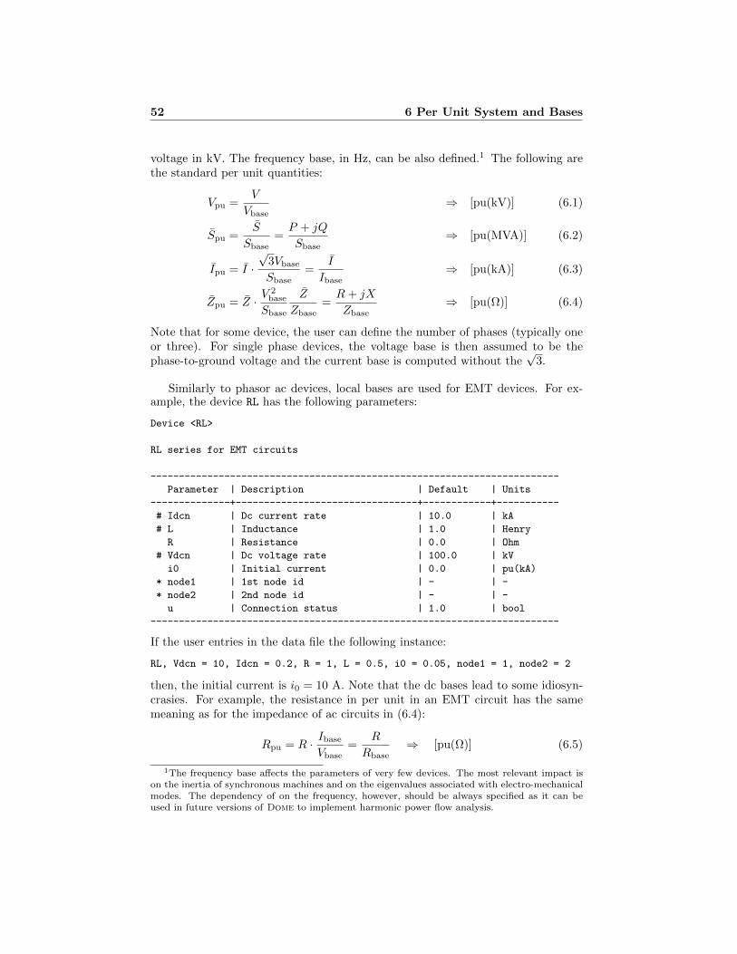
52 6 Per Unit System and Bases
voltage in kV. The frequency base, in Hz, can be also defined.1 The following arethe standard per unit quantities:
Vpu =V
Vbase⇒ [pu(kV)] (6.1)
Spu =S
Sbase=
P + jQ
Sbase⇒ [pu(MVA)] (6.2)
Ipu = I ·√3Vbase
Sbase=
I
Ibase⇒ [pu(kA)] (6.3)
Zpu = Z · V2base
Sbase
Z
Zbase=
R+ jX
Zbase⇒ [pu(Ω)] (6.4)
Note that for some device, the user can define the number of phases (typically oneor three). For single phase devices, the voltage base is then assumed to be thephase-to-ground voltage and the current base is computed without the
√3.
Similarly to phasor ac devices, local bases are used for EMT devices. For ex-ample, the device RL has the following parameters:
Device <RL>
RL series for EMT circuits
------------------------------------------------------------------------
Parameter | Description | Default | Units
--------------+--------------------------------+------------+-----------
# Idcn | Dc current rate | 10.0 | kA
# L | Inductance | 1.0 | Henry
R | Resistance | 0.0 | Ohm
# Vdcn | Dc voltage rate | 100.0 | kV
i0 | Initial current | 0.0 | pu(kA)
* node1 | 1st node id | - | -
* node2 | 2nd node id | - | -
u | Connection status | 1.0 | bool
------------------------------------------------------------------------
If the user entries in the data file the following instance:
RL, Vdcn = 10, Idcn = 0.2, R = 1, L = 0.5, i0 = 0.05, node1 = 1, node2 = 2
then, the initial current is i0 = 10 A. Note that the dc bases lead to some idiosyn-crasies. For example, the resistance in per unit in an EMT circuit has the samemeaning as for the impedance of ac circuits in (6.4):
Rpu = R · IbaseVbase
=R
Rbase⇒ [pu(Ω)] (6.5)
1The frequency base affects the parameters of very few devices. The most relevant impact ison the inertia of synchronous machines and on the eigenvalues associated with electro-mechanicalmodes. The dependency of on the frequency, however, should be always specified as it can beused in future versions of Dome to implement harmonic power flow analysis.

53
However, in per unit, the inductance becomes a time constant.2 In fact, one has:
Lpu = L · IbaseVbase
=L
Rbase⇒ [s] (6.6)
and, hence, it is quite different from the inductance in ac circuits. Similarly, thecapacitance in per unit has the dimensions of a time constant in EMT circuits:
Cpu = C · Vbase
Ibase= C ·Rbase ⇒ [s] (6.7)
In Dome, each device defines its own local power (or current in case of EMTdevices) and voltage bases, there is the need of uniforming all pu values to commonbases.
As in most power system software tools, the user can define a system-wide three-phase ac power base (by default, 100 MVA) and a system-wide dc current base (bydefault, 10 kA). There is also a system-wide frequency, which by default is 60 Hz.
Then ac and dc voltage bases are defined based on voltage rates of the topo-logical devices Bus and Node, respectively. It is up to the user to define consistentvoltage bases for all buses and nodes. For example, the sending- and receiving-endbuses of transformers should have voltage rates consistent with the transformernominal voltages. On the other hand, most EMT devices are connected to twonodes, which should normally have same voltage rates.
If the user explicitly define all bus and node bases and all device nominal pa-rameters, per-unit values are computed as expected. However, it may be lengthyto define all voltage nominal rates of transmission lines, especially if these are thesame as those of buses. With this aim, the set up of data file can be simplified byusing the implicit base definition supported by Dome. This works as follows.
Power and current bases are implicitly the default system bases, e.g., 100 MVAfor three-phase ac devices and 10 kA for EMT devices. The definition of voltagebases of Bus and Node devices is mandatory. Then, all other devices inherit thevoltage base of the bus or node to which they are connected. For example:
Bus, idx = 1, Vn = 200
PQ, bus = 1, p = 1, vmax = 1.05
means that the active power of the PQ load is 100 MW and that its maximumallowable voltage is 210 kV.
Dome provides also a quite unique feature, that is the possibility to define lo-cal power rates for assigned sections of the network. That is, some part of thesystem can use a power base of 100 MVA and another part of the system can use
2This explains why, for example, L is used a time constant of the differential equation (2.7) ofthe current it,d in Chapter 2.

54 6 Per Unit System and Bases
a power base of 1 MVA. With this aim, Bus devices allow defining local powerbases through the local parameter Sn. However, to avoid unexpected results, bydefault, Dome always uses the system ac power base, unless Settings.usepbaseis set to False. Similarly, Dome always uses the system dc current base, un-less Settings.useibase is set to False. Since forcing using local bases can leadto unexpected results, a warning is displayed in case the user provides a customsystem-wide power base and enforce using local bus power bases.
Hot Tip – To connect regions with different power bases require special deviceswhich operate similarly to what transformers do with voltages. These special de-vices are AreaCoup and TransfCoup. The latter is a kind of generalized transformerand allows defining different power and the voltage bases at sending and receivingends.
6.1 Examples
This section provides some examples on the usage of Dome system and devicebases.
Example 1
Assume that Settings.mva = 100 (MVA).
Bus, Vn = 400.0, idx = 1, name = ’Bus1’
Bus, Vn = 400.0, idx = 2, name = ’Bus2’
PQ, bus = 1, p = 0.9, q = 0.6
Then, the power base is 100 MVA and the load powers are referred to that powerbase.
Example 2
Assume that Settings.mva = 100 (MVA).
Bus, Vn = 400.0, idx = 1, name = ’Bus1’
Bus, Vn = 400.0, idx = 2, name = ’Bus2’
Slack, bus = 2, v0 = 1.0
Then, the voltage rate of the slack bus is 400 kV and the slack bus desired voltageis referred to that base.
Example 3
Assume that Settings.mva = 100 (MVA).

6.1 Examples 55
Bus, Sn = 100, idx = 1, name = ’Bus1’
Bus, Vn = 400.0, idx = 2, name = ’Bus2’
Slack, bus = 2, v0 = 1.0
This does not work because the voltage base has to be defined by the device Bus
(mandatory!).
Example 4
Assume that Settings.mva = 100 (MVA).
Bus, Vn = 400.0, Sn = 120, idx = 1, name = ’Bus1’
Bus, Vn = 400.0, idx = 2, name = ’Bus2’
Slack, bus = 2, v0 = 1.0
This does not work because it is not allowed to have different power bases (thepower base of Bus 2 is 100 MVA), unless we use special interfaces that allowsconnecting areas with different power bases.
Example 5
Assume that Settings.mva = 100 (MVA).
Bus, Vn = 400.0, Sn = 120, idx = 1, name = ’Bus1’
Bus, Vn = 400.0, Sn = 120, idx = 2, name = ’Bus2’
PQ, bus = 2, p = 1.0, q = 0.6
The code above is correct but what will be the values of p and q after the conversionon system bases?


Chapter 7
Plotting Results
Dome provides an utility to plot results of time domain simulation, continuationpower flow analysis, as well as any other Dome results that produces a .dat anda .lst file. This utility is invoked with the command dome plot and is a quiteversatile tool based on Matplotlib1 for 2D plots and Mayavi for 3D surfaces. dome
plot also provides a simple calculator2 and a mini-language to perform severaladvanced operations.
7.1 Basic Usage
The simplest command to plot results is:
>> dome plot [options] filename.dat [filename.lst] x y1 [y2 y3 ...]
where filename.dat and filename.lst are the output files of Dome, and x andy1 are the indexes of the variables that one want to be plotted. The first variableindex is used for the horizontal axis, while all remaining variable indexes are usedfor the vertical one. Any number of vertical axis indexes can be provided.
7.1.1 Variable List
Dome creates a default .lst with the same name as the .dat file. The default.lst file is used by dome plot if the user does not provide one explicitly. However,the user can provide a custom .lst file, as long as the format is the same as the.lst file generated by Dome, which is as follows:
• Each line must contain five values separated by colons.
• The first value is the variable index (starting from 0).
• The second value is the variable name.
1To obtain optimal results, Matplotlib has to be configured to enable LATEX commands.2The calculator is based on Sympy.
57

58 7 Plotting Results
• The third value is the variable name formatted in LATEX.3
• The fourth value is the variable unit.
• The fifth value is the variable base (1 if it is not in pu).
The third column is used by dome plot for axis labels and legends. Clearly, theuser can customise the text of the third column as desired. An excerpt of a typical.lst file is as follows:
0, Time, $\rm Time$, s, 1.0000
1, delta Syn 1, $\delta_Syn 1$, rad, 1.0000
2, omega Syn 1, $\omega_Syn 1$, pu(Hz), 1.0000
3, e1q Syn 1, $e\’_q_Syn 1$, pu(kV), 69.0000
4, psidl Syn 1, $\psi_dl_Syn 1$, pu(kWb), 0.1830
5, psiql Syn 1, $\psi_dl_Syn 1$, pu(kWb), 0.1830
6, delta Syn 2, $\delta_Syn 2$, rad, 1.0000
7, omega Syn 2, $\omega_Syn 2$, pu(Hz), 1.0000
8, e1q Syn 2, $e\’_q_Syn 2$, pu(kV), 69.0000
9, psidl Syn 2, $\psi_dl_Syn 2$, pu(kWb), 0.1830
10, e1d Syn 2, $e\’_d_Syn 2$, pu(kV), 69.0000
11, psiql Syn 2, $\psi_ql_Syn 2$, pu(kWb), 0.1830
...
To create a custom .lst file from scratch is seldom necessary. However, it mayhappen that one solves a set of simulations for the same system changing only fewparameters or settings. In this case, the user can customise the default .lst file,rename it and use such a file after each simulation without the need of editing the.lst file several times.
7.1.2 Data File
The .dat file is, in general a binary file that contains the values of the variables,stored as double precision floats, in the same order as indicated in .lst file, organ-ised by columns.
It is possible to convert the binary file into a plain ascii file using the option--toascii or to generate plot parsing a plain ascii data file using the option--oldstyle. Further details on these options are given in the next section.
7.2 dome plot Options
In this section, the command line dome plot options are divided into four groups:(i) general options; (ii) plotting options; (iii) special operations options; and (iv)statistical options. The abbreviated option notation is indicated after the extendedoption name. Options arguments are printed in upper case.
3The user can edit this field to obtain custom legends.

7.2 dome plot Options 59
7.2.1 General Options
-h, --help shows the complete list of dome plot options and exit.
-p PATH, --path=PATH Path of the data file. Not needed if filename.dat is inthe current path. Observe that filename.lst must be in the same path asfilename.dat.
-w, --display Disable opening a window containing the plot. This option isactually not needed unless one comments out the line:
matplotlib.use(’PS’)
in the script plot.py. To allow opening front-end windows is disabled bydefault to allow running Dome on remote servers.
-o OUTPUT, --output=OUTPUT Custom output file name. If the input data file isfilename.dat, the default output is filename.eps.
--oldstyle Parse old-style (i.e., ASCII format) data files.
--toascii Convert the binary input data file into ASCII format.
-0, --silent Do not print any message. This option is useful for batch scripting.
-f EXPORT, --export EXPORT Save plot in a specific graphic format. Availableoptions are eps, jpg, png, gif, bmp and tif.
7.2.2 Plotting Options
-l, --legend Add legend to the plot.
-g, --grid Add grid to the plot.
-s STYLE, --style=STYLE Plot style. Allowed values for STYLE are:
c: continuous coloured lines (default)
b: black lines with different styles
s: coloured lines with symbols
k: black line with symbols
a: all grey
--dim=DIM Plot dimension: ¡2D¿ or ¡3D¿. Default is 2D. 3D plot are in beta-versionand might not work on the current version of Dome.
-n NAMES, --names=NAMES Type of names used in the legend. Allowed values forNAMES are:
f: formatted string (typically LATEX-style string or any string providedin the third column of the .lst file).

60 7 Plotting Results
u: unformatted string (or any string provided in the second column ofthe .lst file).
a: anonymous string. Variables called value and numbered startingfrom 1, e.g., value1, value2, etc. This option can be useful if the userwants to process the .eps file in a LATEX document using the PSfragpackage.
-k POSITION, --position=POSITION Legend location. This option only has ef-fect if used along with option -l. Allowed values for POSITION are:
0: best position (default).
1: upper right.
2: upper left.
3: lower left.
4: lower right.
5: right.
6: centre left.
7: centre right.
8: lower centre.
9: upper centre.
10: centre.
-r REFERENCE, --reference=REFERENCE Index of reference angle.
-t TITLE, --title=TITLE text for the title of the figure.
--ylabel=YLABEL Label for the y axes.
--xlabel=XLABEL Label for the x axes.
--xscale=XSCALE Scale x-axis by a factor.
--yscale=YSCALE Scale y-axis by a factor.
--xoffset=XOFFSET Offset of the x-axis.
--yoffset=YOFFSET Offset of the y-axis.
--xmin=XMIN Minimum x-axis value.
--xmax=XMAX Maximum x-axis value.
--ymin=YMIN Minimum y-axis value.
--ymax=YMAX Maximum y-axis value.
--hline=HLINE Dotted horizontal line.

7.3 Advanced Usage 61
--hline2=HLINE2 Another dotted horizontal line.
--vline=VLINE Dotted vertical line.
--vline2=VLINE2 Another dotted vertical line.
--logx Use logarithmic scale of x-axis.
--logy Use logarithmic scale of y-axis.
--fontsize=N Size of the font used in the ticks, axis labels and legend.
--noformat Disable overwriting LATEX formatting on variable labels.
-u, --nounits Disable including units in variable labels.
-e, --nolegunits Disable including units in legend entries.
--noformat Disable overwriting Latex formatting on variable labels.
-c CUT, --cut CUT Discard initial CUT in percentage of the length of input data.
--last Print the last value of the selected quantities.
-r REFERENCE, --reference REFERENCE Index of reference angle that will be sub-tracted to plotted quantities.
7.2.3 Other Options
-i, --integral Integrate y over x.
-d, --derivate Compute dy/dx.
--fftw Discrete Fourier transform.
--stats Plot mean value and standard deviation on top of the strong trajectoriesthat were used to compute the mean and standard deviation. It must beprovided as a separate .dat file generated using domestat (See Chapter 11)for details.
7.3 Advanced Usage
dome plot provides some macros to allow and/or simplify certain operations. Thesemacros are:
• To plot some variables in a range:
>> dome plot [options] filename.dat [filename.lst] x yi:yf

62 7 Plotting Results
where yi and yf are the initial and the final indexes, respectively, of thevariables to be plotted. Note that yi < yf must hold. For example:
>> dome plot filename.dat 0 1:5
is equivalent to:
>> dome plot filename.dat 0 1 2 3 4 5
• To plot some variables in a range with a given step:
>> dome plot [options] filename.dat [filename.lst] x yi:ystep:yf
where yi and yf are the initial and the final indexes, respectively, of thevariables to be plotted, and ystep is the step used to define the series ofindexes. Note that yi < yf must hold. For example:
>> dome plot filename.dat 0 1:2:15
is equivalent to:
>> dome plot filename.dat 0 1 3 5 7 9 11 13 15
• To plot variable from different input files:
>> dome plot [options] filename1.dat [filename1.lst] x1 y11
[y12 y13] filename2.dat [filename2.lst]
x2 y21 [y22 y23] [...]
The user can define any number of input data files. The default output fileis filename1.eps.
• Wild cards can be used for the input file name. For example:
>> dome plot [options] *.dat x y
will plot the variable with index y versus the variable with index x of all .datfiles in the current directory. Wild cards follows standard Unix-like shell rules.Wild cards are particularly useful if used along with statistical options (seeChapter 11 for further details).

7.3 Advanced Usage 63
• To plot the negative of a variable:
>> dome plot [options] *.dat x y-
The minus sign indicates that dome plot has to plot −y rather than y itself.4
This fact is also indicated in the legend if the option -l is used. To avoid thisbehaviour, the option --noformat has to be enforced.
The minus sign is applied only to the variable at which it is assigned. So, thefollowing command:
>> dome plot [options] *.dat x y1- y2 y3 y4-
will plot the negative of the variables with indexes y1 and y4 but not of thosewith indexes y2 and y3.
• To plot the absolute value of a variable:
>> dome plot [options] *.dat x ya
The a letter indicates that dome plot has to plot b · y where b is the base ofthe variable with index y.5 Variable bases are the values defined in the fifthcolumn of the .lst file. So, the user can modify the .lst file and set custombases.
The absolute value is applied only to the variable at which it is assigned. So,the following command:
>> dome plot [options] *.dat x y1a y2 y3 y4a
will plot the absolute value of the variables with indexes y1 and y4 but notof those with indexes y2 and y3.
The absolute value can be used in conjunction with the minus sign, in anyorder. For example:
>> dome plot [options] *.dat x y-a ya-
will plot the absolute value of the negative of the variable with index y twice.
4Observe that the minus sign has to follow the variable index because otherwise it is interpretedas an option by the Python interpreter.
5Observe that the letter a has to follow the variable index.

64 7 Plotting Results
7.4 Calculator
dome plot can be used as a calculator through a simple mini-language. All op-erations supported by the package Sympy are supported. The rules of the mini-language are the following:
• To distinguish between indexes and numbers, indexes must be enclosed insquare brackets.
• Since spaces are used to separate variables, no space is allowed within eachexpression.
For example:
>> dome plot [options] filename.dat x [y1]+[y2] sin(2*[y3])
will plot the sum of the variables with indexes y1 and y2 and the sinus of the variablewith index y3 multiplied by 2. If enforced, the legend will show the function usedto obtain each line of the plot in LATEX format. To avoid this behaviour, the option--noformat must be enforced.
7.5 Note on Matplotlib
To create plots, Dome relies on the excellent Matplotlib package, which is able toprovide high quality graphics. By default, Matplotlib does not enforce the supportfor LATEX expressions. This fact can mess up the plots created by Dome as variablesexpressions are formatted using the LATEX notation.
This behavior can be changed by properly setting up Matplotlib. With this aim,create a the folder .matplotlib in the user home folder. This folder should exist ifMatplotlib has been launched once. Then, create a file called matplotlibrc withinthe folder .matplotlib. A sample of this file can be found on theMatplotlib websiteat:
http://matplotlib.org/users/customizing.html
Then, open the file matplolibrc and add or uncomment the following line:
text.usetex : True
The file matplotlibrc is highly customizable. For example, to change the ratioof the figures, and obtain plot that take less space in the papers, one can use:
figure.figsize : 8, 4.3
figure.subplot.bottom : 0.13
7.6 Example
Refer to Section 2.3 of Chapter 2 for an example of usage of the dome plot com-mand.

Part II
65


Chapter 8
Groups & Categories
8.1 Groups
Dome internally organises devices into groups and categories. Each device canbelongs to only one group, but can be associated to several categories. Whendefining Dome data files, it is important to remember that devices pertaining tothe same group must have different ID. Failing to do so can lead to inconsistentresults especially for devices that are connected to controllers (e.g., synchronousmachines). This rule is certainly satisfied if the input data are in any format otherthan the internal Dome format but the user has to pay particular care when writing.dm files.
The following command lists all groups and devices belonging to such groups:
$ dome man groups
The devices belonging to a specific group can be obtained substituting groups forthe name of the group. For example:
$ dome man WindTurbine
should produce a result similar to the following one:
DOME device groups
<WindTurbine> (49 items)
------------------------------------------------------------------------
Cswt1 Cswt2 Cswt3 Cswt4
Ddsg1 Ddsg2 Ddsg3 Ddsg4
Ddsg5 Ddsg6 Ddsg7 Ddsg8
Ddsg9 Dfig1 Dfig2 Dfig3
Dfig4 Dfig5 Dfig6 Dfig7
Dfig8 Dfig9 PCswt1 PCswt2
PCswt3 PCswt4 PDdsg1 PDdsg2
PDdsg3 PDdsg4 PDdsg5 PDdsg6
67

68 8 Groups & Categories
PDdsg7 PDdsg8 PDdsg9 PDfig1
PDfig2 PDfig3 PDfig4 PDfig5
PDfig6 PDfig7 PDfig8 PDfig9
WTVoid WindFreq WindFreqS WindFreqd
WindFreqpa
Internally, group information is stored in the dictionary system.device groups,which is organized as follows. The keys of the dictionary are the names of thegroups, e.g., WindTurbine. The value associated with each key is an ordered dic-tionary where the keys are the indexes of the devices belonging to the group andthe keys are the names of the devices. For example:
>>> print(system.device groups[’Synchronous’])
OrderedDict([(1.0, ’Syn5d’), (2.0, ’Syn6a’), (3.0, ’Syn6a’),
(4.0, ’Syn6b’), (5.0, ’Syn6b’)])
This structure makes possible, for example, to link a given controller, e.g., an AVR,to any synchronous machine model without knowing a priori the model (and hencethe device name) of the synchronous machine, but only its ID. This also explainswhy the IDs of devices belonging to the same group must be unique. Back to theexample above, an AVR that has to be connected to machine with ID 2, does notneed to know whether such a machine is a model Syn6a. Instead, it will look at thedictionary system.device groups[’Synchronous’] and find out that the machineis modelled by means of the device Syn6a.
8.2 Categories
Besides groups, Dome also internally organized devices into categories. From ahierarchical point of view, categories are on lower level than groups. A device canbelong to several categories but only to one group. Categories are useful to definecertain common behaviours of device sets.
The following command lists all groups and devices belonging to such groups:
$ dome man categories
The devices belonging to a specific category can be obtained substituting categoriesfor the name of the category. For example:
$ dome man Delay
should produce a result similar to the following one:
DOME device categories
<Delay> (46 items)
------------------------------------------------------------------------
Agcd Avr1d BitumenFreqd CGNN

8.2 Categories 69
DAD1 DAD2 DDEdst DDEsaw
DDEsin DDEsqw DerFreqd DerVoltFreqd
DerVoltd Derd FdlFreqd Food
GPss2d LongLine LongLineCoi LossLess
MackeyGlass MarineFreqd NDDE PTg1d
Pantograph Pantograph2 Pss2d Pss2ddst
Pss2dpd Pss2dsaw Pss2dsin Pss2dsqw
Pss2dwam Pss7d Pss7dpd SPssd
SrfPlld SvrPfd Tg1d ThlFreqd
VscFreqd VscPi5 VscPi5bc VscPi5db
WindCurtailTd WindFreqd
Internally, category information is stored in the dictionary system.device categories,which is organized as follows. The keys of the dictionary are the names of the cat-egories, e.g., Delay. The value of each key is a Python set that collects the namesof the devices that are defined in the input data. For example:
>>> print(system.device categories[’Generation’])
’Syn6a’, ’PVgen’, ’Slack’
Categories are used in some algorithms and devices to find out all devices currentlydefined in the input data that belong to a given type and/or have a specific feature,e.g., devices that contain a delay or that define a generator as shown above.


Chapter 9
Meta-Devices
Meta-devices are a particular set of devices that allows customising the behaviourof Dome or of some class of devices. This chapter describes in detail meta-devicescurrently implemented. The complete list of meta-devices can be obtained with:
$ dome man MetaDevice
9.1 Prototype and Model
It is often the case that there are several devices of the same kind sharing the valuesof some of their parameters. The meta-devices Prototype and Model provide twoconvenient ways to redefine default values for a set of devices.
Prototype changes the default values of all following instances of the givendevice. For example, to assign 0.75 to the active power of PQ instances, one canwrite:
Prototype, device=’PQ’, p=0.75
It is important to note that an instance of Prototype affects only the device thatfollows such instance. Moreover, an instance Prototype can overwrite a previousone. Consider the following example:
PQ, idx = 0
Prototype, device=’PQ’, p=0.75
PQ, idx = 1
PQ, idx = 2
Prototype, device=’PQ’, p=0.6
PQ, idx = 3
PQ, idx = 4, p = 0.5
71

72 9 Meta-Devices
PQ loads with indexes 1 and 2 are initialised with p=0.75, while PQ loads with index3 is initialised with p=0.6. The PQ load with index 0 uses standard default values,i.e., p=0. Finally, observe that the PQ loads with index 4 overwrites the defaultvalue assign by Prototype.
The meta-device Model is similar to Prototype, but it alters the default valuesonly of the devices that points to it. Model is similar to the SPICE statement.MODEL, but is more general, as one can define as many Model’s as needed for anydevice of the system. The only requisite is that the definition of the Model in thedata file must precede the devices that point to that Model. Moreover, differentinstances of Model can coexist. Consider the following example.
PQ, idx = 0, model=’PQ2’
Model, idx=’PQ1’, p=0.75
Model, idx=’PQ2’, p=0.6
PQ, idx = 1, model=’PQ1’
PQ, idx = 2, model=’PQ1’
PQ, idx = 3, model=’PQ2’
PQ, idx = 4, model=’PQ2’, p = 0.5
In this case, PQ loads with indexes 1 and 2 are initialised with p=0.75, while PQ
load with index 3 is initialised with p=0.6. The PQ loads with index 0 will usestandard defaults values, i.e., p=0, because it precedes the instance of Model withindex ’PQ2’. Finally, observe that the PQ loads with index 4 overwrites the defaultvalue assign by Model with index ’PQ2’.
Any device can declare a model parameter. If such model exists, it will be usedto redefine default values, otherwise, the parameter model will be ignored.
Model instances can be nested. For example:
Model, idx=’PQ1’, p=0.75
Model, idx=’PQ2’, model=’PQ1’, q=0.3
PQ, idx = 1, model=’PQ1’
PQ, idx = 2, model=’PQ2’
In this case, PQ loads with index 1 is initialised with p=0.75, but the default valueis assigned to the reactive power, e.g., q=0. The PQ load with index 2 is initialisedwith p=0.75 and q=0.3.
9.2 Output
Output allows selecting output variables for continuation power flow analysis andtime domain simulation. The parameters of this meta-device are:
------------------------------------------------------------------------
Parameter | Description | Default | Units

9.2 Output 73
--------------+--------------------------------+------------+-----------
devID | Index of associated device | None | -
devName | Name of associated device | None | -
macro | Macro for selecting a set of | None | -
| variables | |
var | List of variable names | [] | -
------------------------------------------------------------------------
To select a device variable, use the name of such variable.1 For example:
Output, devName=’Syn6a’, var=[’delta’; ’omega’; ’e1d’; ’e1q’]
To select ac bus voltages, set devName = Bus and for var use:
a: voltage phase angle
v: voltage magnitude
For example:
Output, devName=’Bus’, var=[’a’; ’v’]
To select dc node voltages, set devName = node and for var use v for the voltagemagnitudes, i.e.,
Output, devName=’Node’, var=[’v’]
To select flows of series devices, reserved words for var are:
pij: from-to active power flow
pji: to-from active power flow
qij: from-to reactive power flow
qji: to-from reactive power flow
iij: from-to current flow
iji: to-from current flow
sij: from-to apparent power flow
sji: to-from apparent power flow
For example:
Output, devName=’Line’, devID=’Line 2’, var=[’pij’; ’iji’; ’sji’]
If devID is not defined, all transmission lines will be selected, for example:
Output, devName=’Line’, var=[’pij’; ’iji’; ’sji’]
1The list of device variable names can be obtained using the command $ dome -W DeviceName

74 9 Meta-Devices
Output also supports several “macros” that simplifies the definition of certain,commonly used variables. Available macros are:
x : all state variables
y : all algebraic variables
v : all ac bus voltage magnitudes
theta: all ac bus voltage phase angles
delta: all synchronous machines rotor angles
omega: all synchronous machines rotor speeds
p : all active power injections at buses
q : all reactive power injections at buses
pij : all from-to active power flows
pji : all to-from active power flows
qij : all from-to reactive power flows
qji : all to-from reactive power flows
iij : all from-to current flows
iji : all to-from current flows
sij : all from-to apparent power flows
sji : all to-from apparent power flows
For example:
Output, macro=’pij’
Output, macro=’iji’
Output, macro=’sji’
Note macro will select all series devices, e.g., transmission lines and regulatingtransformers, not only transmission lines as in the example above. If the userdefines a macro, devName and devID, if provided in the same instance of Output,are ignored. For example:
Output, macro=’pij’, devName=’Line’
is the same as
Output, macro=’pij’
Wild cards for devName, devID and macro are supported. Examples:

9.3 Tuning 75
devName = "*" matches all devicesdevID = "*" matches all variables of a devicesdevName = "S*" matches all devices beginning with S
devName = "S?n" matches Syn and Sun, but not Syn4macro = "d*" matches all state or algebraic variables
whose name starts with d
If wild cards are used for devName, then devID should also contain wild cards inorder to lead to some matches. If devID = None or is not defined, is considered asynonym of *.
devName can also be the name of a device group. For example:
Output, devName=’Synchronous’, var=[’delta’; ’omega’]
will select δ and ω variables of all synchronous machines defined in the system (thisexample is effectively a synonym of the macros delta and omega).
A data file can include any number of instances of Output, in any order andposition.
9.3 Tuning
Tuning is a meta-device aimed at customising Dome settings through the inputdata file. The Tuning device itself is void and does not define anything. It is justan interface that modifies default Dome settings. Tuning accepts any attribute ofDome settings. Note that this device overwrites any settings passed through the-s command line option as well as the .domerc file. For example:
Tuning, setting="TDS", step="fixed", tstep=0.01
Note that the parameter setting is mandatory. The example above is equivalentto the following code:
TDS, step="fixed", tstep=0.01
Note also that setting subclasses, such as PF.LM and OPF.Ipopt, can be adjustedonly in the settings files passed through the option -s or in the file .domerc. Seealso Section 4.2.
9.4 Basket
The Basket meta-device randomly selects device models from a list (parameterdevlist). The list of devices names and requires to define a label to point to sucha list. Then the user can define devices called label, whose specific model will berandomly chosen at the time of adding the device to the system.
Basket accepts the following parameters:

76 9 Meta-Devices
------------------------------------------------------------------------
Parameter | Description | Default | Units
--------------+--------------------------------+------------+-----------
delta | Amount of variation of | 0.05 | [0, 1]
| relevant parameters | |
devlist | List of device names (should | [] | -
| belong to the same group or, | |
| at least, have similar | |
| parameters) | |
* label | Label to identify following | None | -
| instances of devices to be | |
| randomly selected | |
randomize | Introduce a uniform variation | True | -
| on relevant device parameters | |
------------------------------------------------------------------------
Example:
Basket, label=’MySyn’, devlist=[’Syn5d’; ’Syn6a’; ’Syn6b’; ’Syn4’;
’Syn3’; ’Syn5a’; ’Syn5b’], randomize=False
MySyn, D = 2.0, M = 10.296, Sn = 615.0, Td10 = 7.4, Td20 = 0.03,
Tq20 = 0.033, Vn = 69.0, bus = 1, fn = 60.0, gen = 1,
idx = 1, name = "Syn 1", xd = 0.8979, xd1 = 0.2995, xd2 = 0.23,
xl = 0.2396, xq = 0.646, xq1 = 0.646, xq2 = 0.4
MySyn, D = 2.0, M = 13.08, Sn = 60.0, Td10 = 6.1, Td20 = 0.04,
Tq10 = 0.3, Tq20 = 0.099, Vn = 69.0, bus = 2, fn = 60.0,
gen = 2, idx = 2, name = "Syn 2", ra = 0.0031, xd = 1.05,
xd1 = 0.185, xd2 = 0.13, xq = 0.98, xq1 = 0.36, xq2 = 0.13
MySyn, D = 2.0, M = 13.08, Sn = 60.0, Td10 = 6.1, Td20 = 0.04,
Tq10 = 0.3, Tq20 = 0.099, Vn = 69.0, bus = 3, fn = 60.0,
gen = 3, idx = 3, name = "Syn 3", ra = 0.0031, xd = 1.05,
xd1 = 0.185, xd2 = 0.13, xq = 0.98, xq1 = 0.36, xq2 = 0.13
MySyn, D = 2.0, M = 10.12, Sn = 25.0, Td10 = 4.75, Td20 = 0.06,
Tq10 = 1.5, Tq20 = 0.21, Vn = 13.8, bus = 6, fn = 60.0,
gen = 6, idx = 4, name = "Syn 4", ra = 0.0041, xd = 1.25,
xd1 = 0.232, xd2 = 0.12, xl = 0.134, xq = 1.22, xq1 = 0.715,
xq2 = 0.12
MySyn, D = 2.0, M = 10.12, Sn = 25.0, Td10 = 4.75, Td20 = 0.06,
Tq10 = 1.5, Tq20 = 0.21, Vn = 18.0, bus = 8, fn = 60.0,
gen = 8, idx = 5, name = "Syn 5", ra = 0.0041, xd = 1.25,
xd1 = 0.232, xd2 = 0.12, xl = 0.134, xq = 1.22, xq1 = 0.715,
xq2 = 0.12
Basket, label=’MyAvr’, devlist=[’Avr1’; ’Avr2’; ’Avr3’; ’Avr4’;
’Avr5’; ’Avr6’], randomize=False
MyAvr, Ka = 200.0, Kf = 0.0012, Ta = 0.02, Te = 0.19, Tf = 1.0,
bus = 1, idx = 1, name = "AVR 1", syn = 1, vmax = 2*9.99,
vmin = 0.0

9.5 Custom 77
MyAvr, Ka = 20.0, Kf = 0.001, Ta = 0.02, Te = 1.98, Tf = 1.0,
bus = 2, idx = 2, name = "AVR 2", syn = 2, vmax = 2*12.05,
vmin = -10.0
MyAvr, Ka = 20.0, Kf = 0.001, Ta = 0.02, Te = 1.98, Tf = 1.0,
bus = 3, idx = 3, name = "AVR 3", syn = 3, vmax = 2*1.7,
vmin = 0.0
MyAvr, Ka = 20.0, Kf = 0.001, Ta = 0.02, Te = 0.7, Tf = 1.0,
bus = 6, idx = 4, name = "AVR 4", syn = 4, vmax = 2*2.2,
vmin = 1.0
MyAvr, Ka = 20.0, Kf = 0.001, Ta = 0.02, Te = 0.7, Tf = 1.0,
bus = 8, idx = 5, name = "AVR 5", syn = 5, vmax = 2*2.2,
vmin = 1.0
Basket, label=’MyTg’, devlist=[’Tg1’; ’Tg2’], randomize=False
MyTg, syn = 1
MyTg, syn = 2
In the code above, the device names for the instances of MySyn, MyAvr and MyTg
are randomly chosen among the devlist’s defines in the Basket devices. Theparameter randomize, if True, introduces a uniform variation of amplitude delta
on double precision parameters of the instances of target devices with name label,thus providing a shortcut for the ALTER macro.
9.5 Custom
This meta-device imports on-the-fly user defined devices from a Python modulepassed to Dome as input data. These are the parameters that can be defined:
------------------------------------------------------------------------
Parameter | Description | Default | Units
--------------+--------------------------------+------------+-----------
* device | Name of user defined class | None | -
| where the device is defined | |
instance | Name of the instance of the | None | -
| device class | |
location | Position where to insert the | None | -
| new device in the system | |
| device list | |
* module | Name of the module where the | None | -
| device is defined | |
path | Absolute or relative path | None | -
| where the module is placed | |
------------------------------------------------------------------------
A complete example on the usage of the Custom device is illustrated in Chapter 2and Appendices B and C.

78 9 Meta-Devices
9.6 DefDev and DefLoad
DefDev defines a given device, say DevB, and links it to another given device, sayDevA. The definition of the DefDev in the data file must follow that of devices DevAto which devices DevB will be added. Instances of device DevA that follows theinstance of DefDev will be ignored. Specific parameters of DevB can be passedthrough DefDev.
------------------------------------------------------------------------
Parameter | Description | Default | Units
--------------+--------------------------------+------------+-----------
* devA | Name of the device to be | None | -
| linked | |
* devB | Name of the device to be | None | -
| defined | |
* link | Name of the attribute of | None | -
| <devB> that links to <devA> | |
------------------------------------------------------------------------
For example, let assume that a given data file includes a certain number of syn-chronous machines and that one want to connect to all these machines an AVR,with same parameters by means of DefDev. The required code is as follows.
Syn6a, idx=1, M=2.5, D=0.5
Syn6a, idx=2, M=2.0, D=0.4
Syn6a, idx=3, M=3.5, D=0.25
Syn6a, idx=4, M=3.0, D=0.8
DefDev, devA=’Syn6a’, devB=’Avr1’, link=’syn’, Ka=25, Ta=0.15
A similar meta-device is DefLoad, but it is specially designed for load modelsthat are initialised after the power flow analysis. DefLoad looks for all PQ loadsand instantiates for each of such loads a given post-power flow load model usinga given percentage of the original PQ power consumption. The definition of the¡DefLoad¿ in the data file must follow that of PQ loads. PQ loads that follows theinstance of ¡DefLoad¿ will be ignored. Specific parameters for the post-power flowload can be passed through ¡DefLoad¿.
------------------------------------------------------------------------
Parameter | Description | Default | Units
--------------+--------------------------------+------------+-----------
* device | Name of the post-power flow | None | -
| load model | |
kp | Percentage of active power | 100 | %
kq | Percentage of reactive power | 100 | %
------------------------------------------------------------------------
For example, the following code, add a stochastic Ornstein-Uhlenbeck process toall PQ loads.
PQ, Vn = 11.0, bus = 507, idx = "PQ_1", p = 0.054, q = 0.0194

9.7 Flick 79
PQ, Vn = 38.0, bus = 510, idx = "PQ_2", p = 0.0719, q = 0.0085
PQ, Vn = 10.0, bus = 511, idx = "PQ_3", p = 0.099, q = 0.0146
PQ, Vn = 38.0, bus = 529, idx = "PQ_4", p = 0.1597, q = 0.0233
PQ, Vn = 38.0, bus = 534, idx = "PQ_5", p = 0.0972, q = 0.0116
PQ, Vn = 38.0, bus = 539, idx = "PQ_6", p = 0.1077, q = 0.0029
PQ, Vn = 38.0, bus = 543, idx = "PQ_7", p = 0.0405, q = 0.0058
DefLoad, device = "PQmr", kp = 100, vp = 0.02, vq = 0.02,
h = 0.01, spp = 2.5
9.7 Flick
This meta-device perturbs a “little-bit” a given equilibrium point by modifying bya given amount a certain variable of a certain device. The perturbation is appliedafter solving the power flow analysis and before starting the time domain integra-tion. Flick only has effect on the time domain integration routine.
Flick includes the following parameters:
------------------------------------------------------------------------
Parameter | Description | Default | Units
--------------+--------------------------------+------------+-----------
delta | Amount of the perturbation to | 1e-05 | -
| be applied | |
* device | Name of the device class to be | None | -
| perturbed | |
* devid | Index of the device instance | None | -
| to be perturbed | |
* varname | Name of the variable to be | None | -
| perturbed | |
------------------------------------------------------------------------
The following example, perturbs the rotor speed with index Syn 3 by a quantity10−3 pu(Hz).
Flick, device=’Syn6a’, devid=’Syn 3’, varname=’omega’, delta=1e-3
9.8 NullTime
This meta-device that allows zeroing the dynamic of a state variable of a givendevice. For example:
NullTime, device=’Syn6a’, state=’e1q’
will set to zero the time constant associated to the variables e1q of all instances ofSyn6a, regardless the values of Td10 defined in such instances.

80 9 Meta-Devices
9.9 Perturbation and Routine
The meta-device Perturbation imports on-the-fly user defined perturbation func-tions to be used during time domain simulations. The user defined function mustaccept two input arguments:
1. an instance of the system class; and
2. the current simulation time.
------------------------------------------------------------------------
Parameter | Description | Default | Units
--------------+--------------------------------+------------+-----------
* function | Name of user defined function | None | -
| where the perturbation is | |
| defined | |
* module | Name of the module where the | None | -
| perturbation is defined | |
path | Absolute or relative path | None | -
| where the module is placed | |
------------------------------------------------------------------------
For example, the following file pert.py varies the reference voltage vref0 of thedevice SVR at t = 20 s.
def vref(system, t):
if (t < 20):
system.SVR.vref0[0] = 1.0025
elif ((t >= 20)):
system.SVR.vref0[0] = 1.005
Such file can be included in the data file with the following code:
Bus, Vn = 130, idx = "Bus2", name = "Bus2"
SVR, idx = 1, Kir = 0.20, Kpr = 0.1, Kiv = 0.02,
Kpv = 100, xe = 0.00768, bus = "Bus2"
Perturbation, function = "vref", module = "pert"
The meta-device Routine works similarly to Perturbation. It imports on-the-flyuser defined routines from a Python module passed to Dome as input data. Theuser-defined routine function must accept as unique argument an instance of thesystem class. Routine can be used to test and debug on local computers newalgorithms or new implementations of existing routines without interfering withthe stable versions installed in the main stream.

9.10 Stack and Splash 81
9.10 Stack and Splash
The meta-device Stack defines a set of N identical devices. The user can passto the Stack device all parameters of the device to be defined plus the numberof devices. It is possible to link the devices defined with an instance of Stack toanother set of devices defined with a previous instance of Stack. The parametersof Stack are as follows.
------------------------------------------------------------------------
Parameter | Description | Default | Units
--------------+--------------------------------+------------+-----------
* DevName | Name of the devices to be | None | -
| defined | |
NDev | Number of devices to be | 1 | -
| defined | |
link | Name of the parameter that | None | -
| allows linking current devices | |
| to others | |
stack | Stack ID to which the devices | None | -
| are to be linked | |
------------------------------------------------------------------------
For example, the following data defines 10 identical PQ loads connected to Bus 1:
Stack, idx = 1, DevName = ’PQ’, NDev = 10, bus = ’Bus 1’,
p = 0.1, q = 0.05
Then, to connect a stochastic perturbation to the loads above:
Stack, idx = 2, DevName = ’PQmr’, NDev = 10, stack = 1,
link = ’pqid’, bus = ’Bus 1’, vp = 0.5, vq = 0.5,
spp = 2.5, sqq = 2.5
The number of devices NDev indicated in Stack 2 must be equal or lower than thenumber NDev defined in Stack 1. Otherwise only 10 PQmr devices will be defined.
Splash is very similar to Stack. It defines a set of N identical devices andrandomly connected them to ac buses. The user can pass to the Splash deviceall parameters of the device to be defined plus the number of devices. It is alsopossible to link the devices defined with an instance of Splash to another set ofdevices defined with a previous instance of Splash. Note that this device should bedefined after the definition of all buses. The parameters of Splash are as follows.
------------------------------------------------------------------------
Parameter | Description | Default | Units
--------------+--------------------------------+------------+-----------
BusType | The bus type to which new | Bus | -
| devices are connected, | |
| available options are <Bus>, | |
| <PBus>, <Node>, and <Pin> | |
* DevName | Name of the devices to be | None | -
| defined | |

82 9 Meta-Devices
NDev | Number of devices to be | 1 | -
| defined | |
link | Name of the parameter that | None | -
| allows linking current devices | |
| to others | |
splash | Splash ID to which the devices | None | -
| are to be linked | |
------------------------------------------------------------------------
For example, the following data defines 10 PQ loads randomly connected to as busesof type Bus:
Splash, idx = 1, DevName = ’PQ’, NDev = 10, BusType = ’Bus’,
p = 0.1, q = 0.05
To connect a stochastic perturbation to the loads defined with the instance above,one has:
Splash, idx = 2, DevName = ’PQmr’, NDev = 10, splash = 1,
link = ’pqid’, bus = ’Bus 1’, vp = 0.5, vq = 0.5,
spp = 2.5, sqq = 2.5
The number of devices NDev indicated in Splash 2 must be equal or lower than thenumber NDev defined in Splash 1. Otherwise only 10 PQmr devices will be defined.
9.11 Alacarte
This meta-device allows defining custom devices by composing different existingclasses, e.g., new wind turbine models, and is intended for expert users. The fol-lowing are the parameters of Alacarte meta-devices.
------------------------------------------------------------------------
Parameter | Description | Default | Units
--------------+--------------------------------+------------+-----------
classes | List of classes to be imported | [] | -
* device | Name of the custom device | None | -
loc | Location where to locate the | None | -
| new device in the system | |
| device list | |
modules | List of modules where to find | [] | -
| the given classes | |
u | Status (use 0 to deactivate | 1.0 | bool
| the instance of the custom | |
| device) | |
------------------------------------------------------------------------
The following are relevant remarks on the parameters of the Alacarte meta-device:
• modules is a list containing the path of given classes in the Dome device tree.It can be a single string (also an empty one), in that case, the modules will

9.11 Alacarte 83
be used for all given classes. If modules is a list, it has to contain the samenumber of elements than the classes list. The absolute path dome.devices.
is prepended if missing. Note that the modules have to be defined in theDome tree. If external modules are required, create the new device througha user-defined module and import it using the meta-device Custom.
• classes is a list of class names required to setup the new device. The order ofthe classes matters as the order provided by the user is applied. Class namescannot contain the module name.
• device must be a capitalised string or will be automatically capitalised whendefining the instance of the custom device. It is important to define namesthat are not already in use. Check the availability of the device name usingthe command line option -q.
• loc is the location where to place the new device in the system device list.By default, new devices will be placed right after synchronous machines inthe device list. This is fine for most devices. If a specific location is needed,specify the name of the device before which the custom device have to belocated.
The following example illustrates how to define the DFIG model Dfig4 usingthe a-la-carte meta-device:
ALaCarte, device = "Dfig4new",
modules = ["wind.dfig"; "wind.grid"; "wind.grid";
"machine.common"; "wind.shaft"; "wind.turbine";
"wind.pitch"; "wind.mppt"; "wind.avr";
"wind.governor"; "wind.crowbar"],
classes = ["kernel"; "polar0"; "freq"; "dfigen";
"shaft1"; "turbine2"; "pitch2";
"mpptc"; "avr1"; "gov2"; "crowbar0"]
Then, new devices Dfig4new can be defined in the file as any other Dome device.


Chapter 10
User Defined Devices
Dome supports the definition of user defined devices through cards. Cards havean extension .dmc and can be loaded on the fly by means for the statement CARDin Dome data files. Cards can be also used to create a template device modulethat the user can later on modify and include in Dome as any other standardmodule. Although quite flexible and versatile, the set up of user defined devicesthrough cards has some limitations and should be used only for quickly test deviceprototypes, not as a systematic tool for implementing new models.
10.1 Notation
Defining custom devices consists in providing to a function (hereinafter, the parser)some input data that such function can parse in order to write another function thatactually implements device model. Moreover, the device model requires input data.Before associating number to such data, the user defined model has to indicate whatthese data are.
Thus, defining custom devices requires that the user thinks in a slightly higherlevel than if he/she implemented the device itself.
To avoid confusion, this is the notation used in this chapter:
Words referring to the syntax of the user defined model
keyword : reserved word that are used to indicate a specific action to the parser.
sub-keyword : reserved word the specifies a feature of a keyword. The syntax iskeyword.sub-keyword.
item: the name of an attribute of the device. The syntax is keyword.item. Itemsare internally used as attribute of a Python class. Items have to be validPython variables (e.g., cannot start with a number) and are case sensitive.Initial and trailing underscores have to be used having in mind Python con-ventions.
85

86 10 User Defined Devices
argument : the value to be associated to the left hand side of the statement, namelykeyword, keyword.sub-keyword, or keyword.item. An argument can be anitem, thus indicating an attribute of the device, or an actual value (a number,a string, a Boolean, a comma-separated list, etc.).
statement : any valid sequence of keyword, sub-keyword or item and argument.There are four statement types:
type 1 statement : keyword: argument
where keyword is a scalar or array attribute to which is assigned thevalue argument. argument can be a comma-separated ordered list. Theword None is a valid argument for indicating that the keyword is notused by the current device. Omitting a certain keyword has the sameeffect as declaring:
keyword: None
Type 1 statements are “cumulative”, i.e., arrays can be defined using asequence of type 1 statements. For example:
keyword: arg1, arg2, arg3
and
keyword: arg1
keyword: arg2
keyword: arg3
do the same.
type 2 statement : keyword.sub-keyword: argument
where keyword is a single property with sub-property sub-keyword towhich is assigned the value argument.
type 3 statement : keyword.item: argument
where the value argument is assigned to the property keyword of thedevice attribute item. item has to be an existing device property definedin a previous type 1 statement.
type 4 statement : keyword.item: arg1, arg2, arg3, ...
where the values arg1, arg2, arg3, etc., are assigned to the propertykeyword of the device data or variable item. This statement is used todefine data and variables in a compact way.

10.2 Card File Format 87
10.2 Card File Format
The card is a sequence of statements with a certain order. The remainder of thischapter describes all valid keywords and sub-keywords of card files.
10.2.1 Version Statement
The first line of a card must be the version statement:
# DOME card v1.0 - user defined device
The text after the dash is optional and can be a brief description of the card itself.Further descriptions can be given using comment lines as explained in the nextsub-section.
10.2.2 Comments
Apart from the very first line, any line that begins with a # is a comment and isneglected when parsing cards.
The keyword comment allows including a comment in the resulting device mod-ule. Comments to be included in the preamble of the module, use a type 1 statementsyntax. For example:
comment: this is a comment of the module preamble!
Comments can be also included in any of the following methods through a type2 statement: init, setx0, ecall, ejacs, windup, params, cjacs, scall, sjacs,getidx, and getidx sw. For example:
comment.ecall: this is a comment of the method <ecall>!
10.2.3 Device Name
The first statement must define the device name, through the keyword name:
name: Device Name, type
The string Device Name is the name used within Dome for the new device as wellas the name used in Dome data file to instantiate an element of the device. Thestring defined by Device Name is case sensitive. Following Dome conventions, thedevice name should start with a capitol letter. The string type is optional andindicates the device category. Currently, there are four types: device, demand,series, avr, avrifield, turbine, and dipole. device is the default value, incase type is not given.
device: this is the most general device. It is basically an empty box that can betailored to any need. No predefined parameters are included except for u
(device status), Sn (power rate) and Vn (ac voltage rate).

88 10 User Defined Devices
demand: same as device, but it includes some special functions for loads that areinitialised after power flow analysis and that requires a static PQ load tobe properly initialised. Using this option is not strictly required but helpsreadability. The following properties are set to True: ecall, shunt, andxinit.
series: this option provides a variety of methods and parameters that define astandard series device. The predefined parameters are those of device plus:bus1 (from bus index), bus2 (to bus index), imax (max current flow), pmax(max power flow), smax (max apparent power flow), Vn2 (voltage rate of thereceiving-end bus), fn (frequency rate), and circuit (circuit ID to distinguishparallel branches). The following properties are set to True: ecall, ejacs,pflow, series, flows, and xinit. The indexes of the sending-end bus voltageare afr and vfr for the phase angle and the magnitude, respectively. Theindexes of the receiving-end bus voltage are ato and vto for the phase angleand the magnitude, respectively. These indexes are used also as variablenames within the device equations but can be overwritten using the keywordsa and v.
dipole: this option provides a variety of methods and parameters that define anempty EMT dipole. The predefined parameters are: node1 (from node index),node2 (to node index), Vdcn (dc voltage rate), and Idcn (dc current rate).The following properties are set to True: dcseries, ecall, pflow, cjacs,and xinit. The indexes for the sending-end and receiving-end bus voltagesare v1 and v2, respectively. These indexes are used also as variable nameswithin the device equations but can be overwritten using the keyword v.
10.2.4 Sections
While following statements can be given in a sparse order, it is highly recommendedthat the card is organized in six sections, with the following order:
1. Connectivity
2. Properties
3. Parameters
4. Variables
5. Equations
6. Initial conditions
A detailed description of each section follows.

10.2 Card File Format 89
10.2.5 Connectivity
All connectivity statements are type 1.
buses: a single bus name or a comma separated list of bus names. These namesdefines the indexes of ac buses.
nodes: a single node name or a comma separated list of node names. These namesdefine the indexes of dc nodes.
stagen: this keyword defines the index and the bus of a static generator to whichthe custom device is connected, as follows:
stagen: gen
This connection implies that property.pflow = False and property.xinit
= True (see next section). Moreover, the static generator is removed afterinitialising the custom device. If the keyword stagen is defined, the wordspg and qg are made available for the initialisation of the custom device. Inparticular, pg and qg are the active and reactive power injections, respectively,of the static generator after solving the power flow at the bus indicated inthe statement buses. The device must be connected to a single ac bus andprotected words pg and qg should not be redefined.
staload: this keyword defines the index and the bus of a static load to which thecustom device is connected, as follows:
staload: load
This keyword implies that property.pflow = False and property.xinit =
True (see next section). Moreover, the static load is removed after initialisingthe custom device. The device must be connected to a single ac bus and 4protected words will be included in the device: p0, q0, kp and kq. The lattertwo are input data. The amount of initial load consumption is computed as:
p0 =kp100
ps,0 (10.1)
q0 =kq100
qs,0
where ps,0 and qs,0 are the active and reactive power, respectively, of the staticload (typically a static PQ load) to which the user defined load is connected.
connect: this allows connecting a certain device to devices other than those indi-cated above, use the following statement:
connect: group name, dev index

90 10 User Defined Devices
where group name is the group of the device to which the custom device hasto be connected, and dev index the name of the device index used in thecustom device. For example, if ones wants to define an AVR, this has to beconnected to synchronous machines. Hence one can define:
connect: Synchronous, syn
The group name is case sensitive. The list of all group name can be retrievedusing the command dome -G.
10.2.6 Properties
Properties indicated with a † are only for advanced usage and can be ignored forthe definition of the vast majority of devices. More details on the properties listedbelow are given in Chapter 17.
The following is the list of valid type 1 statements.
doc: brief description (i.e., it must span a single line) of the device.
type: the group to which the device belongs. The list of existing device groups canbe obtained with dome -G All. The default value is Other, but the user isstrongly recommended to explicitly set a group name. Other should be usedonly in the rare circumstance in which the device substantially differs fromany devices currently embedded in Dome.
category: a single category name or a comma-separated list of categories to whichthe device belongs. The list of existing device categories can be obtainedwith dome -C All. The default value is Other, but the user is strongly rec-ommended to explicitly set a group name. Other should be used only in therare circumstance in which the device substantially differs from any devicescurrently embedded in Dome.
hidden:† whether the device can be defined in the data file or not. It can be Trueor False. Default is False.
avatar:† whether the device requires the creation of an avatar when an equivalenc-ing technique is solved. It can be True or False. Default is False.
The following list of type 2 statements describes the property property that hasseveral sub-properties. Each sub-property can take only two values, namely True
or False. The default value is always False, which is used in case the explicitstatement is omitted. In some cases, even if the user does not set to True a sub-property, this is automatically enforced during compilation time. For example, ifthe user defines algebraic or differential equations, ecall is automatically enforced.However, the user should not rely on this “smart” auto-enforcing and has to takecare to carefully define each sub-property.

10.2 Card File Format 91
property.windup: whether the device contains algebraic equations g.
property.pflow: whether the device is used during power flow analysis.
property.shunt: whether the device is a shunt device, e.g., a load.
property.series: whether the device is a series device, e.g., a transmission line.
property.connection:† whether the device is a connection, e.g., a bus, an area,etc.
property.times:† whether the device includes some switching event that shouldbe computed at user defined times. Enforcing this option implies that thedevice contains a method get times that returns a Python set of the timesat which switching events occur.
property.stagen: whether the device is a static generator, e.g., a PV generator.
property.dyngen: whether the device is a dynamic generator, e.g., a synchronousgenerator.
property.mjacs:† whether the device defines elements of the Jacobian matricesgµ and/or fµ used for CPF analysis.
property.dcseries: whether the device is a dc series element.
property.opf: whether the device is used in OPF analysis.
property.obj: whether the device defines an objective function for OPF analysis.
property.delay: whether the device includes time delays or, which is the same,its equations are DDAE.
10.2.7 Data
Data can be defined using a compact notation, as follows:
datum.name: value, doc, unit [, param, [, time]]
where name is the name of the data as it will be used in the equations, value isthe default value, doc is a brief description of the physical meaning of the data,and unit the data units. The optional field param can be only True or False. Ifparam is omitted, it is assumed to be True. Finally time, also optional, is used todefine the time constant associated to a state variable (time constants should notbe associated to algebraic or switching-manifold variables). If time is omitted, isassumed to be equal to 1.
Example:
datum.M: 5.0, inertia constant, kWs/kVA

92 10 User Defined Devices
10.2.8 Other Parameters
The user can define auxiliary quantities and scalar constants through auxiliary
(or service or ancillary) and scalar, respectively. These are defined by type 1statements. The names given in the statements auxiliary and scalar must beunique.
auxiliary: comma-separated list of auxiliary parameters (i.e., computed once) orvariables (i.e., updated at each iteration) of the device.
scalar: this keyword defines a type 3 statement where the sub-keyword is thename of the scalar constant that the user wants to define. For example:
scalar. pi = 3.1416
Then pi can be used in any equation to indicate 3.1416.
10.2.9 Data Properties
This sub-section describes keywords that define some property of the argumentsgiven in the datum statement. Values of following keywords must be a subset ofthose defined by datum.
zeros: comma-separated list of all parameter names that cannot be zero.
powers: comma-separated list of all parameter names that refer quantities whosephysical unit is that of a power.
voltages: comma-separated list of all parameter names that refer quantities whosephysical unit is that of an ac voltage.
currents: comma-separated list of all parameter names that refer quantities whosephysical unit is that of an ac current.
dcvoltages: comma-separated list of all parameter names that refer quantitieswhose physical unit is that of a dc voltage.
dccurrents: comma-separated list of all parameter names that refer quantitieswhose physical unit is that of a dc current.
impedances: comma-separated list of all parameter names that refer quantitieswhose physical unit is that of an impedance.
admittances: comma-separated list of all parameter names that refer quantitieswhose physical unit is that of an admittance.
resistances: comma-separated list of all parameter names that refer quantitieswhose physical unit is that of an resistance.

10.2 Card File Format 93
conductances: comma-separated list of all parameter names that refer quantitieswhose physical unit is that of an conductance.
times: comma-separated list of all parameter names that refer to quantities whosephysical unit is that of a time.
mandatory: comma-separated list of all parameters that must be defined in thedata file.
For example, assuming that the data p0, q0, g0 and b0 have been define byprevious datum statements, the following are valid expressions:
powers: p0, q0
conductances: g0, b0
10.2.10 Retrieve Data from other Devices
To retrieve data from other devices is often required (see also keyword connect inSubsection 10.2.5). This can be done through the following type 3 statement:
retrieve.dev index: data orig, data dest, type
where dev index is the device index name declared in a previous statement connect;data orig is the original data name as defined in the device from which the datahas to be retrieved; data dest is the name of the data as defined in the customdevice (if not declared by the statement data, it is automatically added to the datalist); and type can be matrix or list, depending on whether the data is usedwithin some equation or not, respectively. For example, if one wants to retrieve theinertia constant of a synchronous machines:
retrieve.syn: M, M, matrix
Observe that a connect statement must declare the connectivity index syn beforethe retrieve statement.
10.2.11 Variables and Switching Manifolds
Device variables can be of three types, namely, algebraic, state and slack variables.Moreover, switching manifolds are defined using the same syntax as variables.
The type 4 statement allows a compact definition of variables as follows:
variable.name: tex, doc, unit
where variable is the variable type, name is the variable name as it will be used inthe equations, tex is the LATEX expression for the variable, doc is a brief descriptionof the physical meaning of the variable, and unit the variable units. State variablesallows including the time constant as a forth argument:
variable.name: tex, doc, unit, time constant

94 10 User Defined Devices
The field variable can take the following values: state, algeb, and switch.
Examples:
state.delta: \delta, rotor angle, rad
state.omega: \omega, rotor speed, pu(Hz), M
10.2.12 Connections to Buses and Nodes
Each connection to the external grid has to be associated to variables, as follows:
ac buses: for each ac bus defined through buses, the keywords v and a assign thename of the voltage magnitude and phase angle, respectively. The keywordsv and a are used within type 3 statements. For example, assume that:
buses: bus1, bus2
Then, one can define:
v.bus1: v1
a.bus1: a1
v.bus2: v2
a.bus2: a2
Observe that v1, a1, v2 and a2 are internally used as the indexes of thealgebraic variables in the global algebraic variable vector.
dc nodes: for each dc node defined through nodes, the keywords v assigns the nameof the instantaneous voltage. The keyword v is used within type 3 statement.For example, assume that:
nodes: node1, node2
Then, one can define:
v.node1: vdc1
v.node2: vdc2
Observe that vdc1 and vdc2 are internally used as the indexes of the algebraicvariables in the global algebraic variable vector.

10.2 Card File Format 95
10.2.13 Equations
An equation has to assigned to each state and algebraic variable. Then an activeand reactive power injection has to be assigned to each ac bus and a current injectionhas to be assigned to each dc node. This can be done through type 3 statementswith the following keywords:
g: algebraic equations associated to each algebraic variable defined through thekeyword y.
f: differential equations associated to each state variable defined through thekeyword x.
p: active power injections associated to each algebraic variable defined throughthe keyword buses.
q: reactive power injections associated to each algebraic variable defined throughthe keyword buses.
i: current injections associated to each algebraic variable defined through thekeyword nodes.
Let illustrate the usage of the keywords above through the exponential recoveryload whose equations are:
p = xp/Tp + pt (10.2)
q = xq/Tq + qt
xp = −xp/Tp + ps − pt
xq = −xq/Tq + qs − qt
Let assume that:
buses: bus1
data: ps, qs, pt, qt, Tp, Tq
params: ps, qs, pt, qt, Tp, Tq
v.bus1: v1
a.bus1: a1
x: xp, xq
Then, the device equations are defined by:
p.bus1: xp/Tp + pt
q.bus1: xq/Tq + qt
f.xp: -xp/Tp + ps - pt
f.xq: -xq/Tq + qs - qt
The following remarks are relevant:
1. The sign of the load active and reactive powers is determined as follows:powers (and currents) are positive if consumed by the device, negative ifproduced by the device.

96 10 User Defined Devices
2. Differential equations are naturally associated to the first derivative of thestate variable. Thus, f.xp is associated to xp. On the other hand, algebraicequations can be associated to any algebraic variable, as long as the numberof algebraic equations is equal to the number of algebraic variables.
3. To define equations, the names of the algebraic and state variables are usedexplicitly. For example, xp is considered the state variable xp. When pars-ing the card, Dome automatically converts xp to the correct syntax, e.g.,dae.x[self.xp] where dae.x is the global vector of state variables andself.xp is the array of indexes of the variables xp defined by the device.
4. Variables v1 and a1 have to be defined even if they are not explicitly used inthe device equations.
A special kind of functions are hard limits. There are four hard limit keywords,as follows.
hardlimit: hard limit for algebraic variables. This function limits an algebraicvariables within given upper and lower bounds, as follows:
ymini ≤ yi ≤ ymax
i (10.3)
The syntax is as follows:
hardlimit.yvar: z, varmax, varmin
where yvar must be an algebraic variable name defined by the keyword y.The symbol z indicates the name of a Boolean variable that indicates whetherthe hard limit is binding or not. Moreover yvar is the index of yi. Finally,varmax and varmin are the names of the limits ymax
i and ymini , respectively.
Note that yvar must by defined as an algebraic variable and varmax andvarmin must be matrices (not constants) and must be defined as data orauxiliary parameters.
windup: windup limit for algebraic variables. The usage of ths algebraic windup isas follows. Let assume:
gi = ϕ(y,x)− yi (10.4)
and:ymini ≤ ϕ(y,x) ≤ ymax
i (10.5)
Equations (10.5) compares ϕ with the limits ymaxi and ymin
i and assigns tothe algebraic variable yi the given value ϕ if such upper and lower boundsare not binding, otherwise assigns to the algebraic variable the binding limit.The algebraic equation gi associated with the algebraic variable yi is set to 0if a limit is binding.
The syntax is as follows:

10.2 Card File Format 97
windup.yvar: z, yval, varmax, varmin
where yvar must be an algebraic variable name defined by the keyword y andyval is an valid expression. The symbol z indicates the name of a Booleanvariable that indicates whether the hard limit is binding or not. Moreoveryvar is the index of yi and gi, the value yval is defined by ϕ(y,x) and is afunction of everything but yi. yval is an expression (the same as that definedin gi). Finally, varmax and varmin are the names of the limits ymax
i and ymini ,
respectively. varmax and varmin must be matrices (not constants) and mustbe defined as data or auxiliary parameters.
table: defines a linear piece-wise function. The syntax is:
table.yvar: yval, xlist, ylist
where yvar must be an algebraic variable name defined by the keyword y andyval is a valid expression. xlist and ylist are lists of same length thatdefine the table. xlist and ylist are defined by the table instance andshould be input data of the device (not auxliary parameters).
deadband: dead band for algebraic variables. The usage of the dead band is asfollows. Let assume:
gi = ϕ(y,x)− yi (10.6)
and:
yi = 0 if − db ≤ ϕ(y,x) ≤ db (10.7)
Equations (10.7) compares ϕ with the dead-band limit db and assigns to thealgebraic variable yi the given value ϕ if ϕ is outside the dead band, otherwiseyi = 0. The algebraic equation gi associated with the algebraic variable yi isset to 0 if ϕ is within the dead band.
The syntax is as follows for standard and step dead-bands:
deadband.yvar: z, yval, type, db, offset
where type is either std or step and yvar must be an algebraic variablename defined by the keyword y or an expression. The symbol z indicates thename of a Boolean variable that indicates whether the dead band is bindingor not. Moreover yvar is the index of yi and gi, the value yval is definedby ϕ(y,x) and is a function of everything but yi. yval is an expression (thesame as that defined in gi). Finally, db is the name of the dead band db.
For asymmetrical deadband the format is:

98 10 User Defined Devices
deadband.yvar: z, yval, type, dbmax, dbmin
where type is asym.
Parameters db, offset, dbmax and dbmin must be matrices (not constants)and must be defined as data or auxiliary parameters.
antiwindup: antiwindup limit for state variables. This function locks the statevariable and its first derivative if either the upper or the lower bound isbinding, as follows.
xi =
0 if fi > 0 and xi ≥ xmax
i
fi(x,y) if xmini < xi < xmax
i
0 if fi < 0 and xi ≤ xmaxi
(10.8)
andxmini ≤ xi ≤ xmax
i (10.9)
The syntax is as follows:
antiwindup.xvar: z, varmax, varmin
where xvar must be a state variable name defined by the keyword x. Thesymbol z indicates the name of a Boolean variable that indicates whether thehard limit is binding or not. Moreover xvar is the index of xi and fi. Finally,varmax and varmin are the names of the limits xmax
i and xmini , respectively.
Parameters varmax and varmin must be matrices (not constants) and mustbe defined as data or auxiliary parameters.
delay: constant delay of a state or an algebraic variable, e.g.:
yd(t) = y(t− τ) (10.10)
The syntax is as follows:
delay.var: tau, val
where var must be a state or an algebraic variable name defined by thekeyword x or y. tau is the name of the constant delay and val is the defaultvalue of the constant delay tau.
The variable z is internally treated as it were defined through the keyword auxiliary.Moreover, the parameters varmax and varmin are treated as they were definedthrough the keywords data and params. Hence, the names z, varmax and varmin
must be unique.
10.3 Example 99
10.2.14 Initial Conditions
If the keyword property.xinit is set to True, the user can provide initial valuesfor the algebraic and state variables of the device. If the keyword property.pflow
is set to True, the values are used as initial guesses. Valid keywords are as follows:
y0: the initial value of algebraic variables defined through the keyword y.
x0: the initial value of state variables defined through the keyword x.
a0: the initial value of the voltage phase angles associated to each bus definedthrough the keyword buses.
v0: the initial value of the voltage magnitude associated to each bus or nodedefined through the keywords buses or nodes, respectively.
u0: the initial value of the auxiliary variable defined through the keyword auxiliary.
Fro example, let be:
buses: bus1
y: y1, y2
x: x1
auxiliary: s1
Then initial values can be defined as follows:
v0.bus1: 1.0
a0.bus1: 0.0
y0.y1: 2.13
u0.s1: 3.25*y1
y0.y2: s0 + y1
x0.x1: 0.0
The following remarks are relevant:
1. Initial values can be expressions involving operations among variables andparameters.
2. The order in which initial values are defined in the card matters. If the initialvalue of y1 is required to compute the initial value of s1, then the statementfor y0.y1 must precede that for s0.s1.
10.3 Example
Let consider the classical electromechanical model of the synchronous machine.Differential equations are:
δ = Ωn(ω − 1) (10.11)
ω =1
M
(pm − ev
x′d
sin(δ − θ)−D(ω − 1)
)

100 10 User Defined Devices
where δ and ω are the state variables, v and θ are the voltage magnitude and phaseangle, respectively, at the generator terminal bus, M the inertia constant, D thedamping, x′
d the transient direct-axis reactance and Ωn the system frequency rate inrad/s. Auxiliary variables pm and e are the mechanical power and the emf behindthe reactance x′
d, respectively.The power injections of the machine into the grid are:
p = − ev
x′d
sin(δ − θ) (10.12)
q =v2
x′d
− ev
x′d
cos(δ − θ)
Observe again that the sign of the powers produced by the machine are negative(because they are injected into the grid).
The machine is initialised after solving the power flow. State as well as auxiliaryvariables have to be initialised, as follows:
pm = p0 (10.13)
e =x′d
v0
√p20 +
(q0 +
v20x′d
)2
δ0 = arcsin
(x′d
ev0
)+ θ0
ω0 = 1.0
where the sub-index 0 indicates that the variables are computed at the initial timet = 0.
The following card file sample illustrates how to define the classical electrome-chanical model of the synchronous machine.
# DOME card v1.0 - device card test
# <name> MUST be the first declaration
# make sure that <name> is not already in use as a device name
name: SynEleMec
#### connectivity ####
buses: bus
nodes: None
stagen: gen
#### device properties ####
# device properties should be defined before variables and equations
doc: classical electro-mechanical model of the synchronous machine
type: Synchronous
hidden: False
avatar: False
property.ecall: True
property.ejacs: True
property.windup: False
property.pflow: False
property.xinit: True

10.3 Example 101
property.shunt: False
property.series: False
property.flows: False
property.connection: False
property.times: False
property.stagen: False
property.dyngen: True
property.mjacs: False
property.dcseries: False
property.opf: False
property.obj: False
property.delay: False
property.cjacs: True
#### scalars ####
# add one statement for each scalar you want to define
scalar.Wn: system.Settings.rad
#### parameters ####
# <datum> should be declared before any parameter properties
datum.M: 5.0, inertia constant, kWs/kVA
datum.D: 0.0, damping coefficient, pu
datum.xd1: 2.0, transient reactance, pu(Ohm)
zeros: M
powers: M, D
voltages: None
currents: None
dcvoltages: None
dccurrents: None
impedances: xd1
admittances: None
resistances: None
conductances: None
times: None
auxiliary: e, pm
mandatory: bus, gen
#### variables ####
state.delta: \delta, rotor angle, rad
state.omega: \omega, rotor angular speed, pu(Hz), M
v.bus: v
a.bus: theta
#### equations and initial conditions ####
# equations must be defined after variables
p.bus: -e*v*sin(delta-theta)/xd1
q.bus: v*v/xd1 - e*v*cos(delta-theta)/xd1
f.delta: Wn*(omega - 1.0)
f.omega: (pm - e*v*sin(delta-theta)/xd1 - D*(omega - 1.0))
#### initialization ####
u0.pm: pg
u0.e: xd1*sqrt(pg**2 + (qg + v*v/xd1)**2)/v
x0.delta: asin(pg*xd1/(e*v)) + theta
x0.omega: 1.0

102 10 User Defined Devices
It is possible to convert the file above into a Python module that can be used as astarting point to set up the synchronous machine model and that can be importedusing the Custom meta-device (see Chapters 2 and 9 as well as Appendices B andC). To convert the .dmc file into a Python script, use the command:
$ dome synem.dmc -o card
The command above will generate the file synem card.py, as follows:
"""User-defined device <SynEleMec>"""
from dome.devices.device import device
# import several functions, just in case!
from cvxopt.base import matrix
from dome.extensions.extras import mul, div, sin, cos, exp, log, sqrt
from dome.extensions.extras import spupdate, sdupdate, mupdate
from dome.extensions.extras import asin, acos, atan2, mpow
from dome.extensions.extras import umul, neg, not0
from dome import commons as com
class synelemec(device):
"""classical electro-mechanical model of the synchronous machine"""
def __init__(self, system, name):
super(synelemec, self).__init__(self, system, name)
self._group = ’Synchronous’
self._state.set(’delta’, r’\delta’, ’rotor angle’, ’rad’)
self._state.set(’omega’, r’\omega’, ’rotor angular speed’, ’pu(Hz)’, ’M’)
self._conn.set(’bus’, ’Bus id’, (’a1’, ’v1’), ’Bus’, (’a’, ’v’))
self.set_datum(’M’, 5, ’inertia constant’, ’kWs/kVA’)
self.set_datum(’xd1’, 2, ’transient reactance’, ’pu(Ohm)’)
self.set_datum(’D’, 0, ’damping coefficient’, ’pu’)
self.set_datum(’gen’, None, ’index of the static generator’, ’-’)
self.set_list(’_zeros’, ’M’)
self.set_list(’_powers’, ’D’, ’M’)
self.set_list(’_z’, ’xd1’)
self.set_list(’_auxiliary’, ’e’, ’pm’)
self.set_list(’_mandatory’, ’bus’, ’gen’)
self.set_dict(’properties’,
dyngen = True,
ejacs = True,
xinit = True,
ecall = True,
opf = True,
cjacs = True)
self.Wn = self.system.Settings.rad

10.3 Example 103
def setx0(self, dae):
self.Wn = self.system.Settings.rad
self.set_params()
pg = umul(self.u, self.system.Bus.Pg[self.a1])
qg = umul(self.u, self.system.Bus.Qg[self.a1])
self.system.rmgen(self.gen)
v = dae.y[self.v1]
theta = dae.y[self.a1]
self.e = mul(mul(self.xd1, div(1, v)), (pg**2.0000 + (qg + \
mul(v**2.0000, div(1, self.xd1)))**2.0000)**0.5000)
self.pm = pg
delta = dae.x[self.delta] = umul(self.u, theta + asin(mul( \
mul(mul(pg, self.xd1), div(1, self.e)), div(1, v))))
omega = dae.x[self.omega] = umul(self.u, 1.0000)
def ecall(self, dae):
v = dae.y[self.v1]
theta = dae.y[self.a1]
delta = dae.x[self.delta]
omega = dae.x[self.omega]
mupdate(dae.g, mul(mul(mul(-self.e, v), div(1, self.xd1)), \
sin(delta + -theta)), self.a1, self.u)
mupdate(dae.g, mul(v**2.0000, div(1, self.xd1)) +
mul(mul(mul(-self.e, v), div(1, self.xd1)), \
cos(delta + -theta)), self.v1, self.u)
mupdate(dae.f, mul(self.Wn, -1.0000 + omega), self.delta, self.u)
mupdate(dae.f, self.pm + mul(-self.D, -1.0000 + omega) + \
mul(mul(mul(-self.e, v), div(1, self.xd1)), \
sin(delta + -theta)), self.omega, self.u)
def getidx(self, dae):
dae.ifx += self.delta + self.omega
dae.jfx += self.omega + self.delta
dae.ify += self.omega + self.omega
dae.jfy += self.v1 + self.a1
dae.igx += self.a1 + self.v1
dae.jgx += self.delta + self.delta
dae.igy += self.a1 + self.v1
dae.jgy += self.v1 + self.a1
def cjacs(self, dae):
sdupdate(dae.Fxc,-neg(self.u), self.delta, self.u, -1)
sdupdate(dae.Fxc,-neg(self.u), self.omega, self.u, -1)
spupdate(dae.Fxc, -self.D, self.omega, self.omega, self.u)
spupdate(dae.Fxc, self.Wn, self.delta, self.omega, self.u)
def ejacs(self, dae):

104 10 User Defined Devices
v = dae.y[self.v1]
theta = dae.y[self.a1]
delta = dae.x[self.delta]
omega = dae.x[self.omega]
spupdate(dae.Fx, mul(mul(mul(-self.e, v), div(1, self.xd1)), \
cos(delta + -theta)), self.omega, self.delta, self.u)
spupdate(dae.Fy, mul(mul(-self.e, div(1, self.xd1)), \
sin(delta + -theta)), self.omega, self.v1, self.u)
spupdate(dae.Fy, mul(mul(mul(self.e, v), div(1, self.xd1)), \
cos(delta + -theta)), self.omega, self.a1, self.u)
spupdate(dae.Gx, mul(mul(mul(-self.e, v), div(1, self.xd1)), \
cos(delta + -theta)), self.a1, self.delta, self.u)
spupdate(dae.Gx, mul(mul(mul(self.e, v), div(1, self.xd1)), \
sin(delta + -theta)), self.v1, self.delta, self.u)
spupdate(dae.Gy, mul(mul(-self.e, div(1, self.xd1)), \
sin(delta + -theta)), self.a1, self.v1, self.u)
spupdate(dae.Gy, mul(mul(mul(self.e, v), div(1, self.xd1)), \
cos(delta + -theta)), self.a1, self.a1, self.u)
spupdate(dae.Gy, mul(2.0000*v, div(1, self.xd1)) + mul(mul(-self.e, \
div(1, self.xd1)), cos(delta + -theta)), \
self.v1, self.v1, self.u)
spupdate(dae.Gy, mul(mul(mul(-self.e, v), div(1, self.xd1)), \
sin(delta + -theta)), self.v1, self.a1, self.u)
Note that the code above is not optimised, in particular the expression of equa-tions and derivatives. Moreover, the card mini-language is incomplete and cannotdeal with sophisticated models including events, complex hard-limits, stochasticprocesses, delays, discontinuities, etc. These advanced modelling aspects can beimplemented only directly in Python and are outlined in part in Chapter 17.

Chapter 11
Statistical Analysis ofResults
Dome includes an utility to compute statistical properties of time series, typicallygenerated using the time domain integration routine. This utility is invoked usingthe command dome stats.
dome statsmainly generates graphical output using Matplotlib and shores somecommand line options with the domeplot utility. These options are: --help,--path, --output, --display, --grid, --title, --silent, --xlabel, ylabel,xmin, xmax, ymin, ymax, --fontsize, and --export. The reader is referred toChapter 7 for a description of these options.
Specific dome stats options are described in the remainder of this chapter.
11.1 Mean and Standard Deviation
The two twin options, --mean, abbreviated with -m, and --std, abbreviated with-v, compute the mean and the standard deviation, respectively, of a set of timedomain simulations, typically obtained in parallel using the option -M of Dome,and generate a .dat and a .lst files with the outputs.
Let’s do an example. Assume that we have dynamic file, say stochastic.dm,with inclusion of Ornstein-Uhlenbeck processes in the loads (obtained using PQmr
devices) and that the we generate 500 time domain simulations with the command:
$ dome -M 500 -r tds stochastic.dm
Once the simulation is completed, there will be 500 .dat files as well as 500 .lst filesin the folder where the simulation has been launched.1 The files will be numeratedprogressively as stocastic job0xxx.dat with xxx ranging from 001 to 500 (samenotation for the .lst files).
1The .lst could be less than 500 is some of the simulations did not complete due, for example,to loss of synchronism of some synchronous machine or numerical issues.
105

106 11 Statistical Analysis of Results
0.0 5.0 10.0 15.0 20.0 25.0 30.0
Time [s]
0.997
0.998
0.999
1.0
1.001
1.002
1.003
ω4[pu]
Figure 11.1: 500 stochastic trajectories of the rotor speed of machine 4.
We can plot all trajectories of a given variables with the command:2
$ domeplot stochastic_job*.dat 0 4
which will return a plot similar to the one shown in Figure 11.1. dome stats
allows computing the mean and the standard deviation at every instant of the 500trajectories with the command:
$ dome stats -m -v stochastic_job*.dat 0 4
which will generate two files, namely:
stat_stochastic_job0001.lst
stat_stochastic_job0001.dat
that will contain the trajectories of the mean and standard deviation respectivelyof the 500 trajectories of the rotor speed of machine 4. These two files can be usedwith dome plot as any other .dat and .lst files. Moreover, the option --stat
of dome plot allows plotting the mean and standard deviation on top of the 500trajectories. The command:
2See Chapter 7 for the usage of wild-cards with domeplot.

11.2 Autocorrelation and Covariance 107
0.0 5.0 10.0 15.0 20.0 25.0 30.0
Time [s]
0.997
0.998
0.999
1.0
1.001
1.002
1.003
ω4[pu]
µ
µ± 3σ
Figure 11.2: 500 stochastic trajectories and statistical properties of the rotor speedof machine 4.
$ dome plot --stat -l stochastic_job*.dat 0 4 \
stat_stochastic_job0001.dat 0 1 2
will produce the output shown in Figure 11.2. The plot include the mean, µ, andµ± 3σ, where σ is the standard deviation of the rotor speed.
11.2 Autocorrelation and Covariance
The autocorrelation and the covariance of a time series can be computed using theoptions --aut, abbreviated with -a, and --cov, abbreviated with -c, respectively.This options works on a single trajectory. In the following, we will describe onlythe autocorrelation option as the covariance option work in the same way. Thesyntax is as follows:
$ dome stats -a stocastic.dat 0 4
This will produce an .eps file called 0 aut.eps and a .lst and a .dat file thatcontains the time lag, the process autocorrelation and the theoretical autocorrela-tion. The latter is computed based on the parameters of a distribution provided bythe user. Without additional arguments, the Normal distribution is assumed with

108 11 Statistical Analysis of Results
mean µ = 0, standard deviation σ = 1 and autocorrelation α = 0.0833. The list ofavailable distributions is obtained with the option --helpdist or -D:
$ dome stats -D
These are:
N NormalB3p 3-parameter BetaG2p 2-parameter GammaG3p 3-parameter Generalized GammaIG2p 2-parameter Inverse GaussianLN2p LognormalR1p RayleighTN2p Truncated NormalW2p 2-parameter WeibullGC3o Gram-Charlier expansion of 3rd order
Default parameters of each distribution can be obtained with the option -H. Forexample:
$ dome stats -H W2p
which returns:
DOME settings
Subclass <Stat.W2p>
Weibull distribution - two-parameter continuous probability distribution.
It is named after Waloddi Weibull, who described it in detail in 1951.
---------------------------------------------------------------------------
Parameter | Description | Default
---------------------------------------------------------------------------
alpha | autocorrelation factor | 0.25
scale | scale parameter | 5.244
shape | shape parameter | 2.343
---------------------------------------------------------------------------
The default parameters of each distribution can be modified using a setting file andpassing such a file with the option --setting, abbreviated with -s. For example:
Stat.W2p.alpha = 0.3
Stat.W2p.scale = 7.35
The option --dist, abbreviated with -d, allows using a distribution other than theNormal one. For example:
$ dome stats -d W2p -a stocastic.dat 0 4

11.3 CDF and PDF 109
0 4 8 12 16 20 24Time lag [h]
0.0
0.2
0.4
0.6
0.8
1.0
Autoco
rrelatio
n Fu
nctio
n
Figure 11.3: Theoretical and simulated autocorrelations obtained using an SDE tomodel a 2-parameter Weibull distribution.
The options above can be used to study the properties of SDE, such as the ones de-picted in Figure 11.3). Mathematical details to obtain Figure 11.3) can be found in:
R. Zarate Minano, F. Milano, Construction of SDE-based Wind Speed Models withExponentially Decaying Autocorrelation, Renewable Energy, accepted in March2016, in press.
11.3 CDF and PDF
The cumulative distribution function (CDF) and probability distribution function(PDF) can be plotted along with measurements or simulation results using theoptions --cdf, abbreviated with -C, --pdf, abbreviated with -P, respectively.
The syntax is similar to the autocorrelation and covariance. The user has tospecify the distribution through the -d option; the parameters of the distributionthrough a setting file and the option -s; and the simulation results through a .dat
file. For example:
$ dome stats -d W2p --cdf stochastic.dat 0 4
An example of the output, taken again from the paper above, is shown in Figure11.4.

110 11 Statistical Analysis of Results
0 2 4 6 8 10 12 14Wind speed [m/s]
0.0
0.2
0.4
0.6
0.8
1.0Cu
mulative Distrib
ution Fu
nctio
n
0 2 4 6 8 10 12 14Wind speed [m/s]
0.00
0.05
0.10
0.15
0.20
Prob
ability Den
sity Fun
ction
Figure 11.4: Left panel: process cumulative probability of an SDE that models a2-parameter Weibull distribution and theoretical CDF. Right panel: process prob-ability of an SDE that models a 2-parameter Weibull distribution and theoreticalPDF.
11.4 Distribution Fitting
The --pdf option works also without the -d option. In this case, dome stats willonly plot the probability histogram using the package Seaborn. For example:
$ dome stats --pdf stochastic.dat 0 4
Moreover, a specific distribution can be passed through the option --fit, abbre-viated with -F. The histogram will be plotted along with a PDF fit based on thegiven distribution. Valid distribution names are all those supported by scipy.stats.For example:
$ dome stats --fit=gamma --pdf stochastic.dat 0 4
Again, the histogram and the fitting PDF are plotted with the package Seaborn.

Chapter 12
Reference Frames
Dome supports different frames. These are the standard single-phase phasor rep-resentation equivalent of three-phase ac systems; the rotating dq-frame based onPark transformation; and the spice-like frame for electromagnetic transient (emt)in both absolute and per-unit values. The elements that define the frame to beused are topological nodes. There are as many of such topological elements asframes. Different frames can be linked through special interface devices. Frames,topological elements and interfaces are described in this chapter.
12.1 Phasor Frame
The phasor frame is based on the single-phase, fundamental frequency equivalentof three-phase ac systems. This is the standard frame of transient stability analysisand is adopted in most commercial tools, e.g., CYME, SIMPOW and PSS/E.
The topological element for the phasor frame is the Bus. Each Bus introducesfour quantities, the phasor voltage magnitude v and angle θ, and the active andreactive powers, p and q, respectively. In Dome, these quantities are used for anyanalysis involving the phasor frame. This is somewhat different from other softwaretools, in particular commercial ones, which typically use (v, θ, p, q) for the powerflow analysis but then switch to (v, θ,ℜı,ℑı) for the time domain integration.
For each Bus, the variables are v (with indexes Bus.v) and θ (with indexesBus.a). Then devices connected to buses defines the active and reactive powerinjections at buses. For example, PQ loads impose a constant p and and constantq. More complex devices will define complex functions for the power injections,but the basic functioning is the same as PQ loads. Dome takes care of summing allpower injections up at every bus so that the balance is satisfied. So, each devicethat is connected to a Bus retrieves that indexes Bus.a and Bus.v and stores suchindexes in internal lists. For example, the PQ load stores such indexes in the listsPQ.a and PQ.v. The power consumption is then computed in the function ecall,
111

112 12 Reference Frames
as follows:
def ecall(self, dae):
mupdate(dae.g, self.p, self.a, self.u)
mupdate(dae.g, self.q, self.v, self.u)
where the syntax of the function mupdate is briefly outlined in Chapter 2 and ex-plained in detail in Chapter 17; self represents here the class PQ; dae.g is the arrayof algebraic equations, where the class dae is passed to the function ecall from thecalling routine; and u is a Boolean array storing the information on the connectionstatus of the load. Note that, due to Dome internal notation, the powers to beadded to the array dae.g are positive if consumed (as in the case of the PQ load)and negative if injected into the bus.
Devices connected to multiple buses, such as series devices (e.g., Line) will in-clude as many active and reactive power balances as the number of buses to whichare connected. Most phasor-frame series devices are based on a low level class calledseries which defines the indices self.afr and self.vfr for the voltage phasorangles and magnitudes at the sending-end buses and self.ato and self.vto forthe voltage phasor angles and magnitudes at the receiving end buses.
Since every device updates the array dae.g, the results is that dae.g can benull only if all algebraic constraints as well as all bus power balances are satisfied.
For steady-state analysis, such as power flow, continuation power flow and opti-mal power flow, one bus voltage angle θi per connected network1 is used as referenceangle, hence θi = θref . Typically, such reference is θref = 0 and is defined by thedevice Slack. Note that one can define as many Slack per connected grid, butonly one can be labelled as reference through the parameter slack.
For time domain simulations, if the Slack generator is substituted by a dy-namic generator model, such as a synchronous machine, no explicit reference angleis included in the system. The reference is an ideal synchronous machine that isnot physically connected to any bus. Such machine has also constant speed (typi-cally ω0 = 1 pu). Every synchronous machine is referred to such reference speed.Hence, unless the centre of inertia is enabled by means of Settings.coi = True,synchronous machines rotor angles and bus voltage phasor angles will drift awayafter any disturbance that modifies the power balance. Moreover, one eigenvaluewill be zero, basically indicating that one machine angle equation is redundant.
Note that it is currently impossible to rune a time domain integration for asystem where there is either no on-line synchronous machine or no enabled Slack
1The connectivity of the network is check by Domebe fore solving the power flow analysis andafter every action of the Breaker devices. The connectivity is defined using an efficient algorithmby Goderya, which is based on the connectivity matrix of series connections. For large networks,however, the checking the connectivity can be time-consuming. The user can disable such a checkby imposing Settings.connectivity = False.

12.2 Rotating dq-Frame 113
device.
12.2 Rotating dq-Frame
The rotating dq-frame is an alternative, more general approach than the phasorframe described in the previous section. This frame is enabled by PBus devices,which introduce four quantities: the dq-axis components of the bus voltages, vdand vq, respectively; and the dq-axis components of the currents injected into thebuses, id and iq, respectively. The variables are vd and vq (with indices vd and vq inthe device PBus). Then the current balances are defined by each device connectedto PBus nodes.
Rotating dq-frame devices can be static or dynamic. Static devices are effec-tively equivalent to phasor-frame devices except for the fact that they use rectan-gular coordinates rather polar coordinates. For example, the device PPQ defines aconstant PQ load in the dq-frame. The ecall method looks as follows:
def ecall(self, dae):
vd = dae.y[self.vd]
vq = dae.y[self.vq]
idl = dae.y[self.idl]
iql = dae.y[self.iql]
mupdate(dae.g, idl, self.vd, self.u)
mupdate(dae.g, iql, self.vq, self.u)
mupdate(dae.g, mpmul(vd, idl, vq, iql) + self.p, self.idl, self.u)
mupdate(dae.g, mnmul(vq, idl, vd, iql) + self.q, self.iql, self.u)
where self.idl and self.iql are the indexes of the dq-frame currents of the PPQload; self.vd and self.vq are the indexes of the dq-frame voltages of the busesto which the PPQ loads are connected; and remaining quantities are parameters ofthe PPQ load.
The dq-frame allows to define also models based on Park’s vectors. For example,a dynamic RL load would look like the following:2
def ecall(self, dae):
vd = dae.y[self.vd]
vq = dae.y[self.vq]
ild = dae.x[self.ild]
ilq = dae.x[self.ilq]
# current injections
mupdate(dae.g, -ild, self.vd, self.u)
2This device is implemented in Dome as Pload1.

114 12 Reference Frames
mupdate(dae.g, -ilq, self.vq, self.u)
# current dynamics
mupdate(dae.f, vd + mnmul(ilq, self.x, ild, self.r), self.ild, self.u)
mupdate(dae.f, vq - mpmul(ilq, self.r, ild, self.x), self.ilq, self.u)
where self.r and self.x are in pu. Note that in this case the dq-frame currentsare state variables, defined as:
self._state.set(’ild’, r’i_Ld’, ’d-axis inductor current’, ’pu(kA)’, ’L’)
self._state.set(’ilq’, r’i_Lq’, ’q-axis inductor current’, ’pu(kA)’, ’L’)
where the time constant L is defined as:
self.L = div(self.x, self._Wn_)
where self. Wn is the conventional name of the system base frequency for eachdevice. Note also that the Park’s reference speed used to compute dq-frame quan-tities is assumed to be constant and equal to be the system nominal synchronousspeed in per unit, i.e., ωdq = ω0 = 1 pu.
The following are relevant concluding remarks on the rotating dq-frame.
• The quantities (vd, vq, id, iq) are used for both steady-state and dynamic anal-ysis.
• Similarly to the phasor frame, a reference quantity is needed in the rotatingdq-frame. This is typically the vq component of the bus voltage of the PSlackdevices. For time domain analysis, if the PSlack device is substituted for adynamic generator, the reference is fictitious synchronous machine rotatingat constant synchronous speed with similar consequences as those indicatedfor the phasor frame in the previous section.
• The command dome -C Park lists all rotating dq-frame devices currently im-plemented in Dome. In most cases, such devices have the same name as theequivalent phasor-domain one with an additional P at the beginning.
• It is possible, with certain limitations, to switch automatically a data fileusing phasor-frame devices to dq frame using the following setting:
Settings.park = True
If the command above is included in the data file through the Tuning meta-device or with the overloaded notation Settings, park=True, such a state-ment has to be inserted at the very beginning of the file, right after thepreamble and the title.

12.3 EMT Frame 115
12.3 EMT Frame
Dome includes a fair number of electromagnetic transient (EMT) device models,including simple circuit elements (e.g., RLC, voltage and current sources, filters),electronic devices (e.g., diodes, BJTs, Mosfets), power-electronic converters (e.g.,dc/dc buck and boost converters), and devices for renewable and distributed gen-eration (e.g., PV cells and energy storage systems).
There are two frames for EMT devices, for high- and low-voltage applications.These are described in the following subsections.
12.3.1 High-Voltage EMT Devices
High-voltage (HV) EMT devices are linked to transmission or distribution systemssystems, typically through some interface (see Section 12.4 below). These devicesare connected to Node’s and their quantities are computed in per unit.3
The Node elements define two quantities, namely the voltage and the current,v and i, respectively. The variable is the voltage v, while devices connected to theNode’s impose the balance of the injected currents. For example, the RL deviceslooks like the following:
def ecall(self, dae):
idc = dae.x[self.I]
v1 = dae.y[self.v1]
v2 = dae.y[self.v2]
mupdate(dae.g,-idc, self.v1, self.u)
mupdate(dae.g, idc, self.v2, self.u)
mupdate(dae.f, v1 - v2 - mul(self.R, idc), self.I, self.u)
Actually, the extension dome.extensions.emt defines a function injection thatimplements the current node balances of dipoles, so that the code above can berewritten as:
def ecall(self, dae):
idc = dae.x[self.I]
v1 = dae.y[self.v1]
v2 = dae.y[self.v2]
injection(dae.g, -idc, self.v1, self.v2, self.u)
mupdate(dae.f, v1 - v2 - mul(self.R, idc), self.I, self.u)
All HV-EMT devices are connected to at least two Node’s except for the deviceGround, which provides the reference voltage (by default, v0 = 0). Note that at
3See Chapter 6 for details on how EMT bases are defined and applied.

116 12 Reference Frames
least one Ground must be defined per each connected circuit of EMT devices.4
The following is a simple example of .dm file with HV-EMT devices:
# DOME format version 1.0
Node, idx = 0, Idcn = 1, Vdcn = 10
Node, idx = 1, Idcn = 1, Vdcn = 10
Node, idx = 2, Idcn = 1, Vdcn = 10
Ground, node = 0
IVGsin, node1 = 1, node2 = 0, v = 1.0, phi = -45
R, node1 = 1, node2 = 2, R = 10
R, node1 = 2, node2 = 0, R = 10
The full list of HV-EMT devices can be obtained with the command:
$ dome -C Circuit
12.3.2 Low-Voltage EMT Devices
Low-voltage (LV) EMT devices are connected to Pin’s and typically use absolutevalues for variables and parameters. Similarly to Node’s, each Pin defines twoquantities, the voltage v and the current i. The variable is the voltage, while thecurrent balance is obtained by summing up all current injections by the devicesconnected to each Pin. The reference voltage is defined by EGround, which hasto be defined explicitly for each connected LV circuit. The full list of low-voltageEMT devices can be obtained with:
$ dome -C Electronic
Note that basic circuital elements, such as RLC and voltage sources, share the samemodels of the HV-EMT devices and have also the same name with an additionalE at the beginning. For example, RLC works for high-voltage EMT circuits, whileERLC for low voltage ones. In addition, LV circuits defines electronic devices suchas Mosfets, BJTs and OpAmps.
The following is a simple example of .dm file with LV-EMT devices:
# DOME format version 1.0
Pin, idx = 0, Idcn = 1e-3, Vdcn = 1e-3
Pin, idx = 1, Idcn = 1e-3, Vdcn = 1e-3
Pin, idx = 2, Idcn = 1e-3, Vdcn = 1e-3
4In other words, Dome does not assume that the node 0 is the reference voltage as in spiceand similar software tools.

12.4 Interfaces 117
EGround, pin = 0
EIVGsin, pin1 = 1, pin2 = 0, v = 1.0, phi = -45
ER, pin1 = 1, pin2 = 2, R = 10
ER, pin1 = 2, pin2 = 0, R = 10
LV-EMT devices are aimed at replicating spice-like models of electronic circuits.However, implemented devices are currently far from being a complete mirror ofspice. There is still a lot of work to do.
12.4 Interfaces
Dome provides several interfaces between two different reference frames. Theseinterfaces are implemented by through special devices. This section describes themall.
12.4.1 Phasor-to-Phasor Interfaces
Apart form the local voltage base, which is mandatory, Bus’es can also define a localpower base and a local frequency base. If these local bases are not defined, the sys-tem bases defined in Settings.mva and Settings.freq are used. Note, however,that the local power and frequency bases do not need to be unique. Different buses,in fact, can define different bases. This can be useful if the system is composed ofareas with very different voltage levels and, hence, different power levels and, morerarely, different frequency bases. It is up to the user to define consistent data wherethe Bus’es have consistent voltage, power and frequency bases. While transformersare the usual physical component aimed at connecting areas with different voltagebases and power electronic converters can couple areas with different frequencies,there is no such a physical device to connect areas with different power bases. Insummary, Dome defines four interfaces:
1. Line and all regulating transformers (see output of the command dome -G
TReg): physical devices that connects two buses (and, hence, two areas) withdifferent voltage bases. For example:
Bus, idx=1, Vn=220, Sn=100, fn=50
Bus, idx=2, Vn=110, Sn=100, fn=50
Line, bus1=1, bus2=2, r=0.02, x=0.1
2. AreaCoup: virtual device that connects two buses (and, hence, two areas)with different power bases. For example:

118 12 Reference Frames
Bus, idx=1, Vn=220, Sn=100, fn=50
Bus, idx=2, Vn=220, Sn=50, fn=50
AreaCoup, bus1=1, bus2=2
3. TransfCoup: generalized transformer that connects two buses (and, hence,two areas) with different voltage and power bases. For example:
Bus, idx=1, Vn=220, Sn=100, fn=50
Bus, idx=2, Vn=110, Sn=50, fn=50
TransfCoup, bus1=1, bus2=2, r=0.02, x=0.1
4. CycloConv: simplified model of a cyclo-converter that connects two areaswith different frequencies. For example:
Bus, idx=1, Vn=220, Sn=100, fn=50
Bus, idx=2, Vn=110, Sn=100, fn=16.7
CycloConv, bus1=1, bus2=2, kt=2
Note that it is not necessary to define the values of the voltage, power and/orfrequency bases in the interfaces. These data, in fact, are grabbed from the busesto which such devices are connected. It possible, however, to define local voltagebases in Line, regulating transformers, TransfCoup and CycloConv, but such basescannot differ more than few percent from the values defined in the buses. Finally,areas with different bases can be also connected through AC/DC devices. Theseare described in Subsection 12.4.5 below.
12.4.2 Single-to-Three-Phase Phasor Interface
The standard phasor-frame devices assume a single-phase, fundamental frequency,balanced equivalent of a three-phase system. Dome, however, allows indicatingwhether the buses and, hence, all connected devices are actually one of the threephases of the three-phase system.5 It is also possible to connect standard single-phase three-phase equivalents to truly three-phase circuits through a device calledFortescue. The following example illustrates how the interface works.
# DOME format version 1.0
Bus, Vn = 400.0, idx = 1, name = "Bus1", region = 2
Bus, Vn = 400.0, idx = 6, name = "Bus6", region = 2
5Note that the three-phase system is not complete as transformer groups, neutral conductors,and “genuinely” three-phase devices are currently not implemented.

12.4 Interfaces 119
Bus, Vn = 230.0, idx = 7, name = "Bus7", region = 2, phase = "a"
Bus, Vn = 230.0, idx = 8, name = "Bus8", region = 2, phase = "b"
Bus, Vn = 230.0, idx = 9, name = "Bus9", region = 2, phase = "c"
Fortescue, bus1 = 6, busa = 7, busb = 8, busc = 9,
r1=0.001, x1=0.025, g1=0, b1=0.005
Line, Vn = 400.0, Vn2 = 400.0, b = 0.01, bus1 = 1, bus2 = 6,
fn = 60.0, idx = "Line_1", name = "Line 1", pmax = 0.3, r = 0.02,
smax = 999.09, x = 0.05
PQ, Vn = 230.0, bus = 7, idx = "PQ_4", name = "PQ Bus7", p = 0.32, q = 0.19
PQ, Vn = 230.0, bus = 8, idx = "PQ_5", name = "PQ Bus8", p = 0.29, q = 0.21
PQ, Vn = 230.0, bus = 9, idx = "PQ_6", name = "PQ Bus9", p = 0.30, q = 0.23
Slack, Vn = 400.0, bus = 1, busr = 1, idx = "Slack_1", name = "Slack Bus6",
pg = 1.4, pmax = 999.9, pmin = -999.9, qmax = 1.5, qmin = -1.5
The Fortescue is effectively a model of a transformer with internal short-circuitimpedance. On the primary winding, the model is a single-phase equivalent, whileon the secondary winding the model is a three-phase system. Since on the single-phase side the system is assumed to be balanced, only the positive sequence passthrough the transformer. Negative and zero sequences are computed to estimatedthe error introduced by neglecting unbalanced conditions on the primary winding.
12.4.3 Phasor-to-dq-Frame Interface
A Bus and a PBus can be linked together through the interface series connectionB2P. This works effectively as a lossless connection that converts the voltage inpolar coordinates into the voltage in rectangular ones; and the complex power intoa current. The ecall function of this interface is reported below.
def ecall(self, dae):
v = dae.y[self.v]
self.sa, self.ca = sincos(dae.y[self.a])
self.vsa = mul(v, self.sa)
self.vca = mul(v, self.ca)
vd = dae.y[self.vd]
vq = dae.y[self.vq]
ild = dae.y[self.ild]
ilq = dae.y[self.ilq]
mupdate(dae.g, self.vsa - vd - mul(self.kd, ild), self.ild, self.u)
mupdate(dae.g, self.vca - vq - mul(self.kq, ilq), self.ilq, self.u)

120 12 Reference Frames
mupdate(dae.g, -ild, self.vd, self.u)
mupdate(dae.g, -ilq, self.vq, self.u)
mupdate(dae.g, mpmul(vd, ild, vq, ilq), self.a, self.u)
mupdate(dae.g, mpmul(vq, ild,-vd, ilq), self.v, self.u)
12.4.4 Hybrid Devices with a Phasor-to-dq-Frame Interface
Although not particularly efficient, dynamic Park’s vector models can be also im-plemented in the phasor frame. These hybrid devices are connected to Bus nodesbut internally define vd and vq components. For example, the dynamic RL load inthe hybrid frame looks like the following:6
def ecall(self, dae):
v = dae.y[self.v]
sincos(dae.y[self.a], self.sa, self.ca)
vd = dae.y[self.vd]
vq = dae.y[self.vq]
ild = dae.x[self.ild]
ilq = dae.x[self.ilq]
# power consumption
mupdate(dae.g, mpmul(ild, vd, ilq, vq), self.a, self.u)
mupdate(dae.g, mpmul(ild, vq,-ilq, vd), self.v, self.u)
# interface equations
mupdate(dae.g, mul(v, self.sa) + vd, self.vd, self.u)
mupdate(dae.g, mul(v, self.ca) - vq, self.vq, self.u)
# current dynamics
mupdate(dae.f, vd + mpmul(ilq, self.x,-ild, self.r), self.ild, self.u)
mupdate(dae.f, vq - mpmul(ilq, self.r, ild, self.x), self.ilq, self.u)
where both voltage and currents in the dq frame are defined as local variables:
self._state.set(’ild’, r’i_Ld’, ’d-axis inductor current’, ’pu(kA)’, ’L’)
self._state.set(’ilq’, r’i_Lq’, ’q-axis inductor current’, ’pu(kA)’, ’L’)
self._algeb.set(’vd’, r’v_d’, ’d-axis bus voltage’, ’pu(kV)’)
self._algeb.set(’vq’, r’v_q’, ’q-axis bus voltage’, ’pu(kV)’)
and a interface has to be implemented between polar coordinates (v, θ) and rect-angular ones (vd, vq).
The command dome -C HybridPark lists all rotating dq-frame devices currentlyimplemented in Dome. In most cases, such devices have the same name as the
6This device is implemented in Dome as HyPLoad1.

12.4 Interfaces 121
equivalent dq-frame one with an additional Hy at the beginning. Note that hybridphasor-dq-frame devices are not recommended for heavy-duty simulations. Theycan be useful, however, comparison and model-checking on small test systems.
12.4.5 Phasor-to-HV-EMT Interface
Currently the only interfaces between the phasor and EMT frames are provided bypower electronics converters. There is currently no interface to transform a phasorquantity into a sinusoidal one and vice versa.
Power electronic converters are effectively ac/dc devices. Dome implementsrelatively simple average, fundamental frequency models of both the ac single-phase equivalent and dc EMT sides. Ac/dc Models currently available can beobtained with the command dome -C AC/DC. These are Inverter, Rectifier,VSC am series, VSC am shunt, VSC dq series, and VSC dq shunt.
The Inverter and Rectifier models have to be used together and implementa thyristor-based HVDC system. The following code defines a 2-terminal HVDCsystem with a dc transmission line:
Bus, Vn = 400.0, area = 2.0, idx = 1, name = "Bus1"
Bus, Vn = 400.0, area = 2.0, idx = 2, name = "Bus2"
Node, idx = 0, Vdcn = 350, Idcn = 0.3
Node, idx = 1, Vdcn = 350, Idcn = 0.3
Node, idx = 2, Vdcn = 350, Idcn = 0.3
Ground, node = 0, v0 = 0.0, Vdcn = 350
RL, node1 = 1, node2 = 2, R = 20, L = 35.0, Vdcn = 350, Idcn = 0.3
Rectifier, idx = 1, bus = 1, node1 = 1, node2 = 0, Vn = 400, Sn = 100,
Vdcn = 350, Idcn = 0.3
Inverter, idx = 1, bus = 2, node1 = 2, node2 = 0, Vn = 400, Sn = 100,
Vdcn = 350, Idcn = 0.3
HVDC_control, rectifier = 1, inverter = 1, iref = 0.15,
node = 1, Vdcn = 350, Idcn = 0.3, vref = 1.15
VSC-based converter are described in the following publications:
N. Chaudhuri, B. Chaudhuri, R. Majumder, and A. Yazdani, Multi- terminaldirect-current grids: modeling, analysis, and control. John Wiley & Sons,2014.
A. Ortega and F. Milano, Generalized model of VSC-based energy storagesystems for transient stability analysis, IEEE Transactions on Power Systems,in press.
The usage of the VSC device is illustrated in Chapter 2. See also the AppendicesB and C for an example including VSC devices.

122 12 Reference Frames
12.4.6 HV-EMT-to-HV-EMT Interface
The interfaces between the high-voltage EMT frames are provided by power elec-tronics dc/dc converters. The models currently available can be obtained with thecommand dome -C DC/DC. These are Chopper, Buck, and Boost. The latter twoinclude the dynamics of the capacitor and the inductor that compose the convertermodel. These models are effectively quadripoles that connects two Node’s withvoltage and current bases, say Vdcn1 and Idcn1, to other two Node’s with voltageand current bases, say Vdcn2 and Idcn2. The following code fragment shows theusage of dc/dc converters.
Node, idx = 1, Vdcn = 20, Idcn = 5, voltage = 1.0
Node, idx = 2, Vdcn = 20, Idcn = 5, voltage = 0.0
Node, idx = 3, Vdcn = 10, Idcn = 10, voltage = 1.0
Node, idx = 4, Vdcn = 10, Idcn = 10, voltage = 0.0
Boost, node1i = 3, node2i = 4, node1o = 1, node2o = 2,
Vdcn = 10, Vdcn_out = 5, lock = 0, d0 = 0.5
Ground, node = 2
Ground, node = 4
Note that both EMT sections linked by the dc/dc converter require an explicitdeclaration of Ground to set the reference voltage.
12.4.7 HV-EMT-to-LV-EMT Interface
The interface Ele2emt device links together a circuit section using HV-EMT devicesto another section using LV-EMT devices. The interface is, effectively, a quadripolelinking two Node’s and two Pin’s. The interface is lossless and simply converts thevoltage and current in absolute quantities on the LV-EMT side into the pu quantitieson the HV-EMT side. The following is a simple code fragment that illustrates thefunctioning of Ele2emt.
Node, idx=1, Vdcn=1m, Idcn=1m
Node, idx=2, Vdcn=1m, Idcn=1m
Pin, idx=1
Pin, idx=2
Ele2emt, node1=1, node2=2, pin1=1, pin2=2

Part III
123


Chapter 13
Installation
13.1 Running Dome from a Remote Terminal
Dome has been designed to be mainly a program for Linux servers. The easiestway to run Dome is to obtain an account on the server with a working version ofDome. Some current locations where Dome is installed are the following Linuxservers:
• faraday1.ucd.ie
• psat.ucd.ie
• tesla.uclm.es
• faraday.uclm.es
13.2 Python Version
Dome runs on Python 3.x. Older version of Python are not supported. Dome isdeveloped and designed for Unix-like 64-bit platforms (e.g., Linux and Mac OS X),but a minimal working version can be compiled on 32-bit platforms as well as onWindows.
13.3 Compiling Dome from Scratch
While installing Dome through the rpm is the recommended way to have a end-userworking version on Fedora Linux, the development of Dome requires the ability ofcompiling sources and extensions. This section describes how to create a develop-ment version of Dome on various platforms.
125

126 13 Installation
13.3.1 Installation on Linux
The installation procedure described in this subsection covers Linux, Unix andMac OS X with MacPort. The procedure to properly compile and link all externallibraries is complex and time consuming. This subsection describes only a minimalbut fully functional version of Dome. This installation requires SuiteSparse, BLAS,LAPACK and GSL libraries.
The procedure described here refers to Linux CentOS 7 64 bit, but it can beeasily applied to any Unix-like OS.
We assume that CentOS 7 64 bit is installed using default options. If installingfrom scratch, it could be useful to include some software packages using SoftwareSelection tag. Within the Software Selection page select the following options:
• On the left side: Gnome Desktop or Server with GUI
• On the right side: Development Tools, Remote Desktop Clients and InternetApplications
If the Linux distribution is already installed, one should take care of install somesoftware development packages. These vary from distro to distro, but, in most cases,will be installed automatically when installing the main dependencies of Dome.
The best practice is to install Dome in the home folder of the user that will bethe main developer of the software. It can also be a fictitious user, say dome, thatcan be accessed by all users that are authorised to modify Dome sources.
On CentOS, it is necessary to enable EPEL Repository in RHEL/CentOS. Thisis not necessary on other Linux distros such as Fedora or Ubuntu, nor on Mac OSX. To download the EPEl repository, execute the command:
# wget http://dl.fedoraproject.org/pub/epel/7/x86_64/e/epel-release-7-2.noarch.rpm
Then install the repo as root:
# yum install epel-release-7-2.noarch.rpm
At this point, it is time to install the following packages using yum (or dnf on recentversion of Fedora):1
python3-devel
python3-setuptools
python3-matplotlib
python3-cvxopt
sympy
numpy
scipy
arpack*
atlas-devel
atlas-static
lapack-devel
gsl*
1On Ubuntu, development packages do not have the -devel suffix. Refer to the synaptic
package to install required libraries and header files.

13.3 Compiling Dome from Scratch 127
Optional but strongly recommended packages are:
python3-networkx
python3-xlwt
python3-xlrd
python3-lxml
python3-progressbar
python3-paramiko
It is important to install all Python packages above for Python version 3. Thelatter package above, python3-paramiko is required only by the utility domever
(see Chapter 14).If some of the Python packages above are not available as a precompiled package,
they can be compiled and installed manually. Using a web browser, go to the PythonPackage Index (https://pypi.python.org/pypi) and download the latest tarballversion of the required Python packages. Then, uncompress the tarballs, enter inthe folders of each package and, for each one, run as root:
# python3 setup.py install
The cvxopt package is the most critical one as it depends on several mathematicallibraries. The good news is that, if the cvxopt package can be installed successfully,also Dome can be installed.
In the home folder of the user that will be the main Dome developer, say/home/developer, create the folder:
$ mkdir Apps
Copy the Dome tarball in the folder Apps and uncompress it.Download from the webpage:
http://faculty.cse.tamu.edu/davis/SuiteSparse/
the tarball SuiteSparse-4.5.3.tar.gz. Then uncompress the downloaded file inthe folder Apps. Download from the webpage:
abel.ee.ucla.edu/cvxopt
the tarball cvxopt-1.1.8.tar.gz. Then uncompress the downloaded file in thefolder Apps and change the name of the folder as cvxopt.
At this stage, there should be three folders:
/home/developer/Apps/dome
/home/developer/Apps/SuiteSparse
/home/developer/Apps/cvxopt
Using a terminal, execute:
$ cd /home/developer/Apps/dome

128 13 Installation
Depending on the Linux distro and OS, it may be required to edit the file setup.py.Open this file with your preferred text editor and make sure that the followingvariables (at the beginning of the file) are set as follows:
ATLAS_DIR = ’’
SSPARSE_DIR = ’../SuiteSparse’
CVXOPT_DIR = ’../cvxopt’
If the libraries above are in different folders, edit the file setup.py as required.At this point, Dome should be ready and can be installed with the command:
# python setup.py develop
The option develop is required to enable the developer mode, i.e., changing thesource code in the /home/developer/Apps/dome folder will be automatically en-abled without the need of repeating the installation procedure. However, if nomodifications to the Dome source code are required or if Dome has to executedby different users, it is recommended to install Dome as follows:
# python setup.py install
If the installation completes successfully, Dome can be now launched using:
$ dome
13.3.2 Installation on Windows 7 64-bit
Download and install Cygwin64. The installer is available at:
https://cygwin.com/setup-x86_64.exe
The installer selects only a basic set of programs and system utilities. Severalextra packages are required to run Dome. If disk space is not a problem, install thewhole Devel, Math, Python, Science and Utils sections and all their dependencies.Check that the following packages are selected:
python3
blas
gsl
lapack
arpack
gcc
gfortran
freetype
png
Install also development files whenever available, e.g., gsl-devel.After the installation the CygWin main folder, say C:\cygwin64, will include a
typical Unix tree, with folders like usr, lib, bin, and home.Launch the Cygwin terminal and install the following packages using easy install-
3.4:

13.3 Compiling Dome from Scratch 129
Figure 13.1: CygWin installer.
setuptools
numpy
scipy
sympy
matplotlib
cvxopt
paramiko
lxml
networkx
xlrd
xlrt
Some of the above might be have already installed during the CygWin setup.
If cvxopt installed properly, then the installation of Dome should also go smoothly.Otherwise solve all compilation and dependency issues generated by cvxopt beforemoving to the next step.
Create a folder, say apps, in the user home folder. Then copy and uncompress tothis folder the dome tarball, the latest distribution of SuiteSparse and cvxopt. Cur-rent versions are SuiteSparse 4.5.3 and cvxopt-1.1.8. These are certainly compatiblewith Dome.
The folder tree should thus contain the following:
./apps/dome
./apps/cvxopt
./apps/SuiteSparse

130 13 Installation
Figure 13.3 shows the symbolic links used for the cvxopt and SuiteSparse folders.The installed version of cvxopt and the version present in the folder apps are the
Figure 13.2: Forlder apps and symbolic links to relevant library sources.
same.Move to the ./apps/dome folder and run:
$ python3 setup.py develop
or
$ python3 setup.py install
The latter installs dome for all users but needs to be launched every time Domesource code is updated.
The setup.py should already be defined for the CygWin environment, but itwill work only if the position of all libraries is the default one. If not, edit thesetup.py file to indicate the right position of required dependencies.
If the installation completes successfully, Dome should be available on the sys-tem. Launching dome at the prompt should produce the result below. It is possiblethat during the execution, Dome crashes due to some missing dependency of DomeC extensions. Python messages are not very informative, as they simply state “Im-port Error: no such file or directory” referred to some extensions. The followingcommand helps define missing libraries:
$ cygcheck.exe ‘pwd‘/name_of_python_C_extensions.dll
where pwd and name of python C extensions are the names of the folder and theDome C extension, respectively.
Once missing libraries are identified, one has to relaunch the CygWin installerand update the installation.

13.3 Compiling Dome from Scratch 131
Figure 13.3: Dome output on the CygWin terminal.
13.3.3 Alternative Installation on Windows 7 32 bit
This subsection describes an alternative procedure to install Dome on Windows 7.This procedure has been tested specifically for the 32 bit version.
The first step is to install Python 2.7.2 and all Dome Python dependencies.Always choose the 32 bit version of the package. For most of the Dome Pythondependencies there exists either a Windows precompiled installer or a Python egg.Both methods are fine as long as all Dome dependencies are properly installed
Then install the latest versions of MinGW and GNU Octave. MinGW is theGNU compiler for the Windows system. GNU Octave is a free clone of Matlab.GNU Octave per se is not needed by Dome, but since GNU Octave comes withmost mathematical libraries precompiled using MinGW, installing GNU Octave isthe fastest and safest way to get BLAS, LAPACK, GSL, and ARPACK without theneed of compiling them from scratch.
It is highly recommended to install Python, MinGW and GNU Octave in the mainC folder. In this way, no changes will be needed in the Dome setup.py script. Inany case, avoid folders that contains space or non alphanumeric characters thatmay create issues to the MinGW compiler.
Once the installation of all the packages listed above is completed, there are stilla few step to complete before Dome can be compiled. These are:
1. Add to the Windows PATH environment variable the location of the Python27folder as well as the Python27/Scripts folder.
2. Create in the Python/Lib/distutils folder a file distutils.cfg as follows:
[build]
compiler=mingw32

132 13 Installation
3. Uncompress the Dome source files in a folder with reading and writing per-missions. It is important to note that this folder will be the working folder ofDome, so that this has to be accessible to anyone allowed to make changesto Dome sources.
4. In the same folder as Dome, download and uncompress the latest version ofSuiteSparse.
Open a Windows command prompt or a PowerShell window, move to the Domemain folder and run:
$ python setup.py develop
If everything has been properly installed and the Windows PATH has been properlycustomised, the command should compile all Dome C extensions and produce aworking developing version of Dome that can be launched from any terminal.
Any changes to the Python sources in the Dome folders will be automaticallyavailable at the next execution of Dome. Changes to Dome C extensions requiresre-running the python setup.py develop command.
13.4 Installing the Dome RPM
There exist also a demo version of Dome distributed as an RPM file. This versioncan be installed only on 64-bit architectures running Fedora. Other platforms thatsupport the RPM system can be used, but theDome RPM distribution file is testedonly on Fedora.
The installation can be easily accomplished using yum (or dnf) and running asroot:
# yum install dome-2011[month][day]-[build].fc15.x86 64.rpm
where month, day and build has to be substituted with current release valueswithout square brackets. For example:
# yum install dome-20110722-1.fc15.x86 64.rpm
The RPM file contains information on all dependencies and should install missingones.
If the RPM file is installed using rpm (which is not recommended), one willhave to manually take care of all dependencies. Required mathematical librariesand Python modules, as follows:
Mathematical Libraries: blas, lapack, SuiteSparse, and gsl.
Python Modules: python-setuptools, Numpy, python-matplotlib, and sympy.
The naming convention is the one used in the Fedora 15 database (it may changeon other platforms that supports RPM packages).

13.5 Optional Python Packages 133
Optional, but strongly recommended packages are arpack, fftw3, python-lxml,python-cvxopt, python-blist, python-networkx, Mayavi, python-xlwt, python-xlrd, andpython-progressbar.
Finally, a package that is not currently used but can be needed in future versionsis python-scipy.
Note 1: only the source code of the SuiteSparse package is needed. It is recom-mended to download and expand the latest SuiteSparse tarball in the same folderas Dome. SuiteSparse is available at:
http://www.cise.ufl.edu/research/sparse/SuiteSparse/
Note 2: packages Numpy, python-matplotlib, and sympy are required only forplotting results through domeplot.
Note 3: all packages above should be installed using the latest version availableon the Fedora repositories.
13.5 Optional Python Packages
There are a few optional Python packages that adds additional features to Dome.Some of them have been indicated above, i.e., python3-lxml, python3-blist, python3-networkx, Mayavi, python3-xlwt, python3-xlrd, and python3-progressbar.
Other recommended packages are
• fastnumbers: this package considerably speeds up parsing Dome .dm files.
• graph-tool: this package is used for topological analysis of graphs. See dome/graphic/graphtool.pyfor details and installation instructions.
• paramiko: this package is used for synchronising and updating Dome versionson the servers that store Dome repositories.
• seaborn: this package is used for fitting and plotting PDFs by domestat.
13.6 External Libraries
A minimal working version of Dome requires some basic Python packages, cvxoptand SuiteSparse. In particular, Dome is heavily based on cvxopt for all dense andsparse matrix operations and on SuiteSparse for sparse matrix factorization. FromSuiteSparse, Dome supports KLU (default), UMFPACK, CXSPARSE, SPQR, andCHOLMOD packages.
With the aim of taking advantage of any cutting-edge mathematical packages,Dome can be statically linked to a variety of external libraries, most of whichare not currently included in common Linux repositories and have, thus, to becompiled and linked manually to Dome. These external libraries are dynamicallyand/or statically included into Dome C extensions.
The libraries currently supported by Dome are:

134 13 Installation
ARPACK Library written in FORTRAN for eigenvalue analysis. ARPACK is avail-able on most Linux distributions.
EISPACK Library written in FORTRAN for eigenvalue analysis. EISPACK is avail-able at:
http://www.netlib.org/eispack/
EXPOKIT FORTRAN function to compute the exponential of a matrix. EXPOKITwhich is available at:
http://www.maths.uq.edu.au/expokit/
However, relevant files are included in the Dome distribution and compiledand linked when running the setup.
FEAST Library written in FORTRAN for eigenvalue analysis. FEAST is availableat:
http://www.ecs.umass.edu/~polizzi/feast/
FFTW3 Library for fast Fourier transform calculations. FFTW3 is available onmost Linux distributions and is generally installed with cvxopt.
FMPC Library written in C for Fast Model Predictive Control. FMPC is availableat:
http://stanford.edu/~boyd/fast_mpc/
The Dome wrapper is based on the function fmpc step.c.
GSL GNU Scientific Library. GSL is available on most Linux distributions.
HSL Harwell Subroutine Library (HSL) is a suite of efficient FORTRAN routines.HSL is available at:
http://www.hsl.rl.ac.uk/
The Dome wrapper support some routines for sparse matrix factorizationand eigenvalue analysis.
IPOPT Efficient nonlinear programming solver based on the interior point method.IPOPT is provided by COIN-OR and is available as a RPM package:
coin-or-Ipopt.x86_64
coin-or-Ipopt-devel.x86_64
LUSOL Library written in FORTRAN for LU factorization developed by the Stan-ford University. LUSOL is available at:

13.6 External Libraries 135
http://www.stanford.edu/group/SOL/software/lusol.html
MAGMA Library that provides an implementation of LAPACK routines for het-erogeneous “Multicore + GPUs” architectures. MAGMA is available at:
http://icl.cs.utk.edu/magma/
MPI Parallel interface functions. Dome supports both OpenMPI and MPICH, al-though the former is to be preferred. OpenMPI and MPICH are available onmost Linux distributions.
MUMPS Library written in FORTRAN for sparse matrix factorization. MUMPSis available on most Linux distributions.
NICSLU Library written in C for sparse matrix factorization. NICSLU is availableat:
http://nicslu.weebly.com/
NICSLU2 Library written in C for sparse matrix factorization. This version is notfreely available and must be requested to directly to the authors. NICSLU2can be requested at:
http://nicslu.weebly.com/
PARDISO Library written in FORTRAN for sparse matrix factorization of sym-metric and asymmetric matrices. PARDISO is available at:
http://www.pardiso-project.org/
PETSc Library for parallel Krylov subspace factorization of sparse matrices. PETScis available at:
www.mcs.anl.gov/petsc/petsc-as/
SLEPc Library for parallel computing the eigenvalues of sparse matrices (based onPETSc). SLEPc is available at:
www.grycap.upv.es/slepc/
SLICOT Library written in FORTRAN for advanced control algortihms. SLICOTis available at:
http://slicot.org/objects/software/slicot/slicot.tar.gz
SPOOLES Library written in ANSI C for sparse matrix factorization. SPOOLES isavailable as source code (mailto:[email protected]) or precom-piled RPM file:

136 13 Installation
spooles-2.2-1.fc18.x86_64.rpm
spooles-devel-2.2-1.fc18.x86_64.rpm
SuperLU Library for LU factorization of parse matrices. SuperLU is available at:
http://crd.lbl.gov/~xiaoye/SuperLU/
SuperLU MT Library for distributed LU factorization of parse matrices using amulti-threading approach. SuperLU MT is available at:
http://crd.lbl.gov/~xiaoye/SuperLU/
SuperLU DIST Library for distributed LU factorization of parse matrices usingMPI. SuperLU DIST is available at:
http://crd.lbl.gov/~xiaoye/SuperLU/
TAUCS Library for large (possibly out-of-core) sparse matrix factorization of sym-metric matrices. TAUCS is available at:
http://www.tau.ac.il/~stoledo/taucs/
WSMP the Watson Sparse Matrix Package (WSMP) is a FORTRAN package forsparse matrix factorization. WSMP is available at:
http:
//researcher.watson.ibm.com/researcher/view_project.php?id=1426
Y12M Library written in FORTRAN for sparse matrix factorization of symmetricmatrices. Y12M is available at:
http://www.netlib.org/y12m/
ZPARES Library written in FORTRAN for eigenvalue analysis. ZPARES is avail-able at:
http://zpares.cs.tsukuba.ac.jp/
Detailed instructions to install all extensions above are provided in the pream-bles of the extensions C files included in the folder dome/extensions.
The utility domesup, currently under development, is aimed at simplifying theinstallation procedure, in particular, the setup of licenses and scripts that are re-quired to run certain libraries. Once complete, this utility is intended to providean out-of-shelf installation of all relevant Dome extensions based on third-partylibraries. The current usage of domesup is reserved to superusers, and assumesthat a basic installation of Dome as the ones discussed above is available on the

13.6 External Libraries 137
system.
The on-line help on the functions provided by each wrapper can be obtainedon an interactive Python interpreter by importing the library and the invoking thefunction help. For example:
>>> import dome.extensions.wsmp as wsmp
>>> help(wsmp)
To get the names of available wrappers, execute the following commands on aPython interactive session:
>>> import dome.extensions as ext
>>> help(ext)


Chapter 14
Synchronization and VersionControl
Dome provides the command synch to synchronize the local sources with exter-nal repositories. This command provides functionalities similar to subversion andmercurial.
The remainder of the chapter will assume that Dome sources are installed in afolder, say dome, within another folder, say Apps. dome synch can be successfullyexecuted only if launched from a folder that includes the main Dome folder.
Without any option, dome synch cleans the Dome source tree, updates theversion, creates a new complete Dome tarball and upload it to the servers whereDome repositories are located. Note that to be able to perform the update on theservers one needs the passwords on such servers. The other operations can be doneby any user that access to the Apps folder.
The default behaviour can be customised in several different ways. The followingare the options of the dome synch command.
-h, --help show this help message and exit.
-i, --incremental saves only modified files in the Dome tarball.
-k, --clean clean source-code Dome tree.
--build build RPM.
--chmod change file permissions in the Dome tree (needed only for groups).
--macsetup setup development Dome installation on Darwin OS.
--demo apply modifications to enable demo mode.
--nodemo apply modifications to disable demo mode.
-c, --compare only compares the time stamps of current files with those in thedatabase, no file is modified.
139

140 14 Synchronization and Version Control
-r, --remove removes files that are not included in the database.
-n, --dontaddnew includes files that are found in the local repository but not inthe database.
-t, --timestamp only creates the current time stamps of the files in the Dometree.
-d, --noupload only create the tarball, do not upload it to the servers.
-v, --nonewver create the tarball without updating Dome version.
-l, --local create a local full tarball (implies -v and -d).
-u, --update retrieve the latest Dome tarball and patches and extract them uponthe current repo.
-e, --noexpand do not expand the tarball and patches retrieved.
-m, --noremove do not remove retrieved tarball and patches.
-b, --back restore an older version.
-f, --fork create a differential tarball with recent changes but not update Domeversion.
Of all options above the most commonly used are -i and -u. The former cre-ates an incremental version that includes only changes with respect to the lastsynchronisation and upload the update to the servers. Since only modified filesare stored and uploaded, this options allows significantly saving space (time whileuploading). The other option, -u, updates the version of Dome currently savedon the local machine retrieving all needed full tarballs and/or incremental versionsfrom the firstly available repository. It is a good idea to recompiled and reinstallDome after any execution of dome synch -u, especially is C extensions have beenupdated.
The -l option is also useful to create a local tarball, which will store a snapshotof the current local Dome source code but will not change the version nor updateanything to the repositories.
Particular care has to be taken when executing the options --build, --demoand --nodemo. The correct sequence is:
$ domever --demo
$ domever --build
$ domever --nodemo
This will create a demo RPM file that can be freely redistributed. If dome synch
--demo is not executed before running dome synch --build, the resulting RPMfile will contain a fully-fledged Dome version, which has to be treated confidentially

141
and cannot be redistributed to third parties without my consent. Finally, one hasto launch dome synch --nodemo, otherwise, the local version of Dome will workas a the demo version, i.e., the number of buses and state variables will be limitedat run-time.


Chapter 15
Extension Extras
This chapter describes the Dome extensions extras, which extends the cvxoptdense and sparse matrix operations with a plethora of new and, generally, very effi-cient functions. The complete list of functions provided by extras can be obtainedwith an interactive Python session with the commands:
>>> import dome.extensions.extras as extras
>>> help(extras)
We first describe six functions, namely, massign, mupdate, sdassign, sdupdate,spassign and spupdate, which are particularly important for the definition ofdevice models. A first glance at these functions can be found in Chapter 2. Aknowledge of these functions is required to properly understand next Chapter 17.
massign(...) Replaces in-place the elements of a dense matrix with given vectorand indexes.The syntax is: massign(A, B, I, U), where:
A real dense matrix to be modified.
B input real dense matrix whose elements are used to modify A.
I list or integer dense matrix of the indexes in A where the elements of Bhave to be substituted. I must have the same length as B
U real dense matrix of zeros ans ones with same length as B. If U[i] = 0
the element A[I[i]] is set to zero. Vector U is optional.
This function is utilized mainly to assign the elements of state and algebraicvariables at the initialization step.
mupdate(...) Updates in-place the elements of a dense matrix with given vectorand indexes.The syntax is: mupdate(A, B, I, U), where:
A real dense matrix to be modified.
143

144 15 Extension Extras
B input real dense matrix whose elements are used to modify A.
I list or integer dense matrix of the indexes in A to which the elements ofB have to be added. I must have the same length as B
U real dense matrix of zeros ans ones with same length as B. If U[i] is zerothe element A[I[i]] is not updated. Vector U is optional.
This function is utilized mainly to update the elements of differential andalgebraic equations during iterative procedures, such as the Newton-Raphsonmethod used for power flow analysis and time domain integration.
sdassign(...) Replaces in-place diagonal elements of a sparse matrix with givenvector and index.The syntax is: sdassign(A, B, I, U, offset), where:
A real sparse matrix to be modified.
B input real dense matrix whose elements are used to modify A.
I list or integer dense matrix of the indexes of the diagonal elements of Awhere the elements of B have to be substituted. I must have the samelength as B
U real dense matrix of zeros ans ones with same length as B. If U[i] is zerothe element A[I[i]] is set to zero. Vector U is optional.
offset the value to which A[I[i]] is assigned if U[i] is zero. By default,offset is zero.
This function is utilized mainly to set constant elements of the Jacobianmatrices of differential and algebraic equations during iterative procedures,such as the Newton-Raphson method used for power flow analysis and timedomain integration. In particular, it can be used for those elements of theJacobian matrices that are truly constant, accessed by only one device, andnever null. For example, in the function
T x = f(y, x) = Ky − x
the derivative fx = −1 can be conveniently assigned with sdassign:
sdassign(dae.Fxc, -1, self.x)
sdupdate(...) Updates in-place diagonal elements of a sparse matrix with givenvector and index.The syntax is: sdupdate(A, B, I, U, def), where:
A real sparse matrix to be modified.
B input real dense matrix whose elements are used to modify A.
I list or integer dense matrix of the indexes of the diagonal elements ofA to which the elements of B have to be added. I must have the samelength as B

145
U real dense matrix of zeros ans ones with same length as B. If U[i] is zerothe element A[I[i]] is not modified. Vector U is optional.
def real scalar which is assigned to A[I[i]] in case U[i] is zero.
This function is utilized mainly to set constant and time-varying elements ofthe Jacobian matrices of differential and algebraic equations during iterativeprocedures, such as the Newton-Raphson method used for power flow analysisand time domain integration. In particular, it can be used for those elementsof the Jacobian matrices that can change during the simulation or dependson input data. For example, in the equation
T x = f(y, x) = Ky −Hx
the derivative fx = −H can be conveniently assigned with sdupdate, as H[i]can be zero and hence, if the device is disconnected (i.e., U[i] is zero), thediagonal element cannot be zero:
sdupdate(dae.Fxc, -self.H, self.x, self.u, -1)
Another important case where it is needed to use the function sdupdate is forpure integrators. Let assume that a pure integrator is defined by the equation:
x = Ki(yref − y)
Then, one should include the follwoing statement in the method cjacs:
sdupdate(dae.Fxc, 0, self.x, self.u, -1)
This prevents that the Jacobian matrix is singular in case an instance of thedevice is inactive, i.e., for every item, for which self.u[item] is zero. Notealso that the eigenvalue analysis depends on the value of def. As a generalrule, one should set def to −1 for differential equations and to 1 for algebraicequations.
spassign(...) Replaces in-place the elements of a sparse matrix with given vectorand indexes.The syntax is: spassign(A, B, I, J, U, offset), where:
A real sparse matrix to be modified.
B input real dense matrix whose elements are used to modify A.
I list or integer dense matrix of the indexes of the rows of A where theelements of B have to be substituted. I must have the same length as B.
J list or integer dense matrix of the indexes of the columns of A where theelements of B have to be substituted. J must have the same length as B.
U real dense matrix of zeros ans ones with same length as B. If U[i] is zerothe element A[I[i]] is set to zero. Vector U is optional.

146 15 Extension Extras
offset the value to which A[I[i]] is assigned if U[i] is zero. By default,offset is zero.
This function is utilized mainly to set constant elements of the Jacobianmatrices of differential and algebraic equations, as well as time constant ma-trices (T x and Rx) during iterative procedures, such as the Newton-Raphsonmethod used for power flow analysis and time domain integration. In partic-ular, it can be used for those elements of the Jacobian matrices that are trulyconstant and never null. For example, in the function
T1x1 − T2x2 = f(x1, x2) = Kx2 − x1
the off-diagonal element of the matrix T x, i.e., −T2, can be convenientlyassigned with spassign:
spassign(dae.Tx, -self.T2, self.x1, self.x2)
Note that, when assigning time constants, it is not needed to pass the vectorU.
spupdate(...) Updates in-place the elements of a sparse matrix with given vectorand indexes.The syntax is: spupdate(A, B, I, J, U), where:
A real sparse matrix to be modified.
B input real dense matrix whose elements are used to modify A.
I list or integer dense matrix of the indexes of the rows of A to which theelements of B have to be added. I must have the same length as B.
J list or integer dense matrix of the indexes of the columns of A to whichthe elements of B have to be added. J must have the same length as B.
U real dense matrix of zeros ans ones with same length as B. If U[i] is zerothe element A[I[i]] is not updated. Vector U is optional.
This function is utilized mainly to set constant elements of the Jacobianmatrices of differential and algebraic equations during iterative procedures,such as the Newton-Raphson method used for power flow analysis and timedomain integration. In particular, it can be used for those elements of theJacobian matrices that are time-varying and/or input data dependent. Forexample, in the function
T x = f(y, x) = Ky − x
the time constant fy = K can be conveniently assigned with spupdate:
spupdate(dae.Fy, self.K, self.x, self.y, self.u)

147
Other relevant functions of the extension extras are described in the remainderof this chapter. In the following, unless explicitly stated or implicit in the descrip-tion of the function, it is assumed that the function operates element-wise on denseand sparse matrices. In the examples, lower case letters indicate scalars whereasupper cases (or bold face) letters indicate dense or sparse matrices. All functions,unless explicitly stated, works on double-precision arrays. The support for integerand complex arrays has to be tested case by case and is not indicated, in general,in the descriptions provided below.
acos(...) Returns the element-wise arcosine of a matrix. For example, B =
acos(A).
adjdiff(...) Returns a vector of the difference of adjacent elements of an inputvector (first value is zero). For example, B = adjdiff(A).
adjsum(...) Returns a vector of the sum of adjacent elements of an input vector(first value is zero). For example, B = adjsum(A).
arange(...) Returns an equally spaced vector. For example, A = arange(start,
end, step). See also linspace and logspace.
asin(...) Returns the element-wise arcsine of a matrix. For example, B = asin(A).
atan2(...) Returns the element-wise arctangent of the ratio of two matrices. Forexample, C = atan2(A, B).
bigger(...) Compares two matrices A and B and returns a matrix whose elementsare 1 if A[i] > B[i], 0 otherwise. For example, C = bigger(A, B).
blasname(...) Returns the name of the BLAS library used to compile Dome.Usage: name = blasname().
ceil(...) Returns the element-wise ceil values of a matrix. For example, B =
ceil(A).
checksign(...) Check the value of array A, and set B[i] = 1 if A[i] > 0, B[i]= 0 otherwise. For example, B = checksign(A).
cmul(...) Returns the element-wise product of a real dense matrix by a complexdense matrix. For example, C complex = cmul(A real, B complex).
colnihil(...) Set in-place to a given tolerance a given column of a sparse matrix.For example, colnihil(A, h, tol). By default, tol is 10−24.
conj(...) Returns the conjugate of a matrix. For example, B = conj(A).
cos(...) Returns the element-wise cosine of a matrix. For example, B = cos(A).This is a more efficient implementation of the function cos provided by cvxopt.
cosh(...) Computes the element-wise hyperbolic cosine of a matrix. For example,B = cosh(A).

148 15 Extension Extras
crect(...) Returns a complex vector from its real and imaginary parts. Forexample, C complex = crect(A real, B imag).
ctrue(...) Returns the index of the first nonzero element of the input vector, -1otherwise. For example, h = ctrue(A).
cuda(...) True if CUDA extensions are available. For example, bool = cuda().
cudaver(...) Returns the available CUDA driver version. For example, version= cudaver().
cumsum(...) Returns a vector of the cumulative sum of an input vector. Forexample, B = cumsum(A).
deadband(...) Returns the input value computed through a generalized dead-band. For example, Y = deadband(X, Xmax, Xmin), where X is the inputmatrix, and Xmax and Xmin are the boundaries of the dead-band. The outputis computed as follows: y = x− xmin if x < xmin; y = x− xmax is x > xmax;y = 0 otherwise.
decoldx(...) Returns the a list of row indexes of a given column of a sparsematrix A. For example, rows = decoldx(A, col), where col is an integeror a list of integers. This function is very efficient for cvxopt sparse matriceswhich are stored in CCS format.
decouple(...) Set in-place to zero the columns and the rows of a sparse matrixat given indexes, but for the diagonal elements, which are set to one. Theresulting matrix results thus “decoupled” into as many matrices as the lengthof the index list. For example decouple(A, idx), where idx is an integer ora list of integers. This function is not efficient and should be used only withsmall matrices.
deindex(...) Returns the positions in the value array of the diagonal elements ofa sparse matrix. For example p = deindex(A, idx), where idx is an integeror a list of integers. This function is not efficient and should be used onlywith small matrices.
derowdx(...) Returns the a list of column indexes of a given row of a sparsematrix A. For example, cols = decoldx(A, row), where row is an integer ora list of integers. This function is quite slow for cvxopt sparse matrices whichare stored in CCS format.
div(...) Returns the element-wise division of two dense matrices, i.e., C = A/B.For example, C = div(A, B). This is a more efficient implementation of thefunction div provided by cvxopt.
dplus(...) Returns the element-wise d+ = (z > 0?1 : 0), where z is a real densematrix. For example, B = dplus(A).

149
exp(...) Returns the element-wise exponential of a matrix. For example, B =
exp(A). This is a more efficient implementation of the function exp providedby cvxopt.
eye(...) Returns a dense identity matrix of order n. Optionally, diagonal elementscan be set to a given value. For example, I = eye(n) and A = eye(n, val).Note that n cannot be too large to avoid overflows.
findnext(...) Returns True if the value val is found in a sorted dense real orinteger matrix A and the last position checked.For example, found, pos = findnext(A, val), where found is True orFalse and pos is an integer. Optionally, a starting position can be passed:found, pos = findnext(A, val, start). By default, start is zero.
floor(...) Returns the element-wise floor values of a matrix. For example,B = floor(A).
getjumps(...) Returns the sum of jumps of a Poisson process and updates theindex of such process. The function has the following syntax:
s = getjumps(jumps, times, state\_old, state\_new, t, i)
where:
jumps: vector of jumps magnitudes (real dense matrix).
times: vector of times at which the jumps occur (real dense matrix). timesand jumps must have the same length.
state old: vector of old positions in the vectors jumps and times, i.e., beforesumming the jumps up to time t (integer dense matrix).
state new: vector of new positions in the vectors jumps and times, i.e., aftersumming the jumps up to time t (integer dense matrix).
t: current simulation time (float scalar).
i: process position in the vectors state old and state new (integer scalar)
s: summatory of jump magnitudes in the time interval from the old timeand the current time t.
getnonzero(...) Returns a matrix that contains only the non-zero elements of theinput matrix. So the size of the input and output matrices can be different.For example, B = getnonzero(A).
greater(...) Compares two matrices A and B and returns a list whose elements areTrue if A[i] > B[i], False otherwise. For example, L = greater(A, val).
imp2adm(...) Returns the admittance from the impedance value. For example,G, B = imp2adm(R, X). All arguments must be real dense matrices.

150 15 Extension Extras
inpoly(...) Determines if a given point lays inside or outside a given polygon.The point is provided as a pair of coordinates (x, y), and the polygon isdefined by two matrices, one for the coordinates of points x and one for thecoordinates of points y. The syntax is: u = inpoly(Px, Py, x, y), wherePx and Py are the matrices defining the coordinates of the polygon, and x andy are the coordinates of the point. On output, u is True if the point is insidethe polygon, False if it is outside.
inpolyv(...) Determines if a given point lays inside or outside a given polygon.This function is the vectorized version of inpoly. The points are providedas pairs of coordinates (x, y), and the polygons are defined by two matrices,one for the coordinates of points x and one for the coordinates of pointsy. The syntax is: U = inpolyv(LPx, LPy, X, Y), where LPx and LPy arelists of the matrices defining the coordinates of the polygon, and X and Y
are the matrices containing the coordinates of the points (x, y). The outputis a double-precision matrix whose elements are 1 if the point is inside thepolygon, 0 if it is outside.
interp(...) Computes the linear interpolation of a dense matrix. The syntax is:Y = interp(X, XP, YP), where XP and YP are the original arrays of (xp,yp)value-pairs, X is the new array of x values; and Y is the resulting new arrayof y values.
interpc(...) Computes a point of the linear interpolation of a dense matrix. Thesyntax is: y = interp(x, dx, XP, YP), where XP and YP are the originalarrays of (xp,yp) value-pairs, x is the new value x; dx is the step ∆x, and y
is the resulting interpolated value y.
isany(...) Returns 1 if any element of the input vector is nonzero, 0 otherwise.For example, u = isany(A).
isequal(...) Returns 1 if all elements of the input vector are equal, 0 otherwise.For example, u = isequal(A).
isstring(...) Determines heuristically whether the string contains a string withdelimiters ’ or ". For example, isstring(’5.6234’) returns False, andisstring(’"text"’) returns True. This function is used in the parsers ofdata files.
linspace(...) Returns an equally spaced vector. For example, A = linspace(start,
end, n), where n is the desired number of elements of the output vector A.See also arange and logspace.
log(...) Returns the element-wise natural logarithm of a matrix or a scalar. Forexample, B = log(A). This is a more efficient implementation of the functionlog provided by cvxopt.
log10(...) Returns the element-wise base-10 logarithm of a matrix or a scalar.For example, B = log10(A).

151
logspace(...) Returns a vector whose elements are spaced evenly on a log-10scale. For example, A = logspace(start, end, n), where n is the desirednumber of elements of the output vector A and the range is 10 ** start and10 ** end. See also linspace and arange.
maxabs(...) Returns the maximum of the absolute value of a real dense matrix.For example, r = maxabs(A).
maxmat(...) Returns the element-wise maximum of two dense real matrices. Forexample, C = maxmat(A, B).
mclone(...) Update in-place the elements of a dense matrix A based on anotherdense matrix B. For example, mclone(A, B). On output, A == B and B isunchanged.
mdiv(...) Returns (ab/c), where a, b, and c are real matrices. For example,D = mdiv(A, B, C).
mean(...) Returns the mean value of a matrix or of a sequence of doubles. Forexample, m = mean(A).
memsign(...) Sets in-place the signs of the elements of an array with memoryof old value and tolerance. The function accepts three inputs, A, B, and,optionally, tol. By default, tol is 10−24. The elements of B are updatedonly if the absolute values of the elements of A are greater than tol. Then,the elements of B are set according to the rules of the function sign below.
minabs(...) Returns the minimum of the absolute value of a real dense matrix.For example, r = minabs(A).
mincr(...) Update in-place the elements of a dense matrix a ∈ Rn based on othertwo dense matrices b ∈ Rm and c ∈ Rp, with n = m + p. Then, the first melements of a are replaced with the elements of b and the remaining p elementsof a are replaced with the elements of c. For example, mincr(A, B, C).
minmat(...) Returns the element-wise minimum of two dense real matrices. Forexample, C = minmat(A, B).
mmmul(...) Returns (abcd), where a, b, c and d are real matrices. For example,E = mmmul(A, B, C, D).
mmul(...) Returns (abc), where a, b, and c are real matrices. For example, D =
mmul(A, B, C).
mnmul(...) Returns (ab−cd), where a, b, c and d are real matrices. For example,E = mnmul(A, B, C, D).
mpmul(...) Returns (ab+cd), where a, b, c and d are real matrices. For example,E = mpmul(A, B, C, D).

152 15 Extension Extras
mpow(...) Returns element-wise base A raised to the power exponent B. For ex-ample, C = mpow(A, B).
mround(...) Returns the element-wise rounded to 10−6 values of a real matrix.For example, B = mround(A).
mul(...) Returns the element-wise product of two dense matrices. For example,B = mul(A). This is a more efficient implementation of the function mul pro-vided by cvxopt.
neg(...) Returns NOT(u), where u is a list or a matrix of Boolean’s. For example,B = neg(A).
nihil(...) Sets in-place the elements of a dense or a sparse matrix to a smallvalue. For example, nihil(A).
nihiltol(...) Sets in-place the elements of a dense or a sparse matrix to zero ifbelow a given tolerance. For example, nihiltol(A, tol).
This function can also be utilized to extract statistics from the matrix, withoutactually modifying the matrix itself, as follows: nnz, ratio = nihiltol(A, tol, 0)
returns the number nnz of elements that are above the given tolerance tol
and the ratio between such a number and the size of the matrix, i.e., nnz /
(A.size[0] * A.size[1]). In this case, A is not modified.
nihilval(...) Sets in-place the elements of a dense or a sparse matrix to val ifA[i] < val. For example, nihilval(A, val).
nonzero(...) Define elements and indexes of a dense matrix that are above agiven tolerance.
norm2(...) Returns the element-wise Euclidean norm of two real matrices (c =√a2 + b2). For example, C = norm2(A, B).
not0(...) Returns 1 if u[i] == 0, otherwise returns u[i], where u is a list or adense matrix. For example, B = not0(A).
notnone(...) Returns 0 is the argument is None, otherwise returns the argumentitself. For example, b = notnone(a).
nudiv(...) Divides the negate of a Boolean vector by a matrix. For example, B= nudiv(U, A), where U is a double precision matrix of zeros and ones. Thisis equivalent to B = udiv(neg(U, A)).
numul(...) Multiplies the negate of a Boolean vector by a matrix. For example, B= numul(U, A), where U is a double precision matrix of zeros and ones. Thisis equivalent to B = umul(neg(U, A)).
ones(...) Returns a dense double precision matrix whose elements are all equal to1. The syntax is A = ones(n, m), or A = ones(n), where m = 1 by default.Example: A = ones(3) returns a matrix with 3 rows and 1 column, whoseall 3 elements are equal to 1.

153
pair(...) Splits a string into a pair of values using a given separator character.This function is used by the parser of .dm files. By default the separator is=, e.g., str1, str2 = pair(str0), but a custom separator can be passed tothe function, e.g., str1, str2 = pair(str0, ’,’).
phase(...) Returns the phase in radians given a list of phase letters. The outputis a dense double-precision matrix. Supported inputs are ’a’, ’b’, ’c’. Forexample, A = phase([’a’, ’b’, ’c’]).
polar(...) Returns a polar complex number into rectangular form c = ajϕ. Theinputs are the magnitude a and the phase angle ϕ of the complex number asscalars or real dense matrices. The output is a complex dense matrix. Forexample, C = polar(A, Phi)
prod(...) Returns the product of the elements of an input vector. For example,p = prod(A).
pythagoras(...) Returns (aa+bb−cc), where a, b, and c are real matrices. Forexample, D = pythagoras(A, B, C).
qdiv(...) Safe matrix division (a/b). The syntax is as follows: C = qdiv(A, B,
ref, tol, base), The function returns A[i]/B[i] if B[i] < tol, and ref
otherwise. Optionally, the ratio A[i]/B[i] can be multiplied by base. Bydefault, tol is 10−12 and base is 1. A can be a scalar or a real dense matrix.This function is used to compute the quantised increments of state variablesduring the time domain integration (see option step = ’quantized’ of thesetting class TDS).
qudiv(...) Divides a vector by a matrix, where the vector is mostly composedof zero elements. For example, C = qudiv(A, B). This function should beslightly more efficient than udiv, if the majority of elements of A are zero.
qumul(...) Multiplies a vector by a matrix, where the vector is mostly composedof zero elements. For example, C = qumul(A, B). This function should beslightly more efficient than umul, if the majority of elements of A are zero.
rect(...) Returns a complex vector in polar form. For example, B, C = rect(A),where A is a dense complex matrix and B and C are the magnitude and thephase angle, respectively of A.
rownihil(...) Set in-place to a given tolerance a given row of a sparse matrix.For example, colnihil(A, h, tol). By default, tol is 10−24. This functionis not very efficient for large matrices in CCS format.
saturate(...) Returns 0 if zi < 0, 1 if zi > 1, zi otherwise, where z is a realmatrix. For example, B = saturate(A).
sdiv(...) Safe matrix division A/B. Returns 0 for every null element of B. Forexample, C = sdiv(A, B).

154 15 Extension Extras
select(...) Selects between two lists or matrices based on the value of a Booleanvector. For example, C = select(U, A, B), where U is a double precisionmatrix or list of zeros and ones. This is equivalent to C = umul(U, A) +
umul(neg(U), B).
setref(...) Substitutes the element of reference list to output list if these areNone.
sign(...) Returns the element-wise sign of a matrix, i.e., 1 if A[i] > 0, -1 ifA[i] < 0, and 0 if A[i] == 0. For example, B = sign(A).
sin(...) Returns the element-wise sine of a matrix. For example, B = sin(A).This is a more efficient implementation of the function sin provided by cvxopt.
sincos(...) Returns element-wise sine and cosine values of a matrix. For exam-ple, S, C = sincos(A), where A is the argument value, and, on output, S andC will contain the values of the sine and the cosine of A. Matrices S and C areallocated by sincos. A is not changed. The in-place usage is also supported,i.e., sincos(A, S, C), where S and C are pre-existing matrices of the samelength and type as A.
sinh(...) Returns the element-wise hyperbolic sine of a matrix. For example, B= sinh(A).
skew(...) This function substitutes in place a real dense square matrix A with itsskew, namely:
A(i,j) if i > j
A(i,i) = 0
A(i,j) = -A(j,i) if i < j
For example, skew(A).
slicing(...) Replaces the elements of an array of length m with the first melements of another array. For example, slicing(A, B). Optionally, anoffset of B can be given, slicing(A, B, offset).
spclone(...) Updates the elements of a sparse matrix based on another sparsematrix. The two matrices are assumed to have same sizes and non-zero pat-tern. For example, spclone(A, B) will substitute the elements of A with theelements of B.
spcopy(...) Returns the copy of a sparse matrix. For example, B = spcopy(A).
speye(...) Returns a sparse identity matrix of order n. Optionally, diagonalelements can be set to a given value. For example, I = speye(n) andA = speye(n, val).

155
spfastrep(...) Replaces given elements of the input sparse matrix with a givenvalue. For example, spfastrep(A, I, val) will substitute the elements of Awith val at the positions I, where I is a dense integer matrix with the indexesof the elements to be substituted as obtained by the function spindex.
spindex(...) Returns the indexes of the elements of a sparse matrix within an-other sparse matrix. For example, I = spindex(A, B, ioff, joff) willfind the indexes in the buffer of A of the elements of B, which is assumedto be a submatrix of A. ioff and joff indicate the row and column offsets,respectively, in matrix A. ioff and joff are optional and by default are 0.The output I is a dense integer matrix. This function is used to map Jacobianmatrices fx, fy, gx and gy into the full Jacobian matrix Ac of the system.
spmerge(...) Merges the elements of a sparse matrix based into another sparsematrix. The two matrices are assumed to have same sizes but not necessar-ily same non-zero pattern. For example, spclone(A, B) will substitute theelements of A with the elements of B. The elements of A that are not in B areunchanged.
spmuldiag(...) Multiplies a sparse matrix A by a vector B assuming that thevector is a diagonal matrix. For example, C = spmuldiag(A, B). The resultC is a sparse matrix.
spmuldiop(...) Multiplies in-place a sparse matrix A by a vector B assuming thatthe vector is a diagonal matrix. For example, spmuldiag(A, B). The resultis stored in A. This is the in-place version of the function spmuldiag.
spmulvec(...) Multiplies a sparse matrix by a dense column vector. For example,C = spmulvec(A, B). The result is stored in the dense vector C.
spnewmat(...) Create a new sparse matrix from index lists and include diagonalelements if not defined in the lists of indexes.The syntax is: C = spmulvec(val, I, J, n), where val is the value towhich the elements of the sparse matrix C have to be initialized, I and J
are the lists of indexes of the non-zero elements, n is the size of the matrixC. Optionally, diagonal elements can be initialized to val + ref, if a fifthargument ref is included: C = spmulvec(val, I, J, n, ref). By default,ref is zero.
spreplace(...) Replaces given elements of the input sparse matrix A with the ele-ments of another sparse matrix B. For example, spreplace(A, B, I), whereI is a dense integer matrix obtained with the function spindex. This func-tion is used to replace the system Jacobian matrix Ac with the elements ofJacobian matrices fx, fy, gx and gy.
spsumdiop(...) Sums in-place a sparse matrix A and a vector B assuming thatthe vector is a diagonal matrix. For example, spmuldiag(A, B). The resultis stored in A.

156 15 Extension Extras
spsumming(...) Adds in-place given elements of the input sparse matrix B tothe elements of another sparse matrix A. For example, spreplace(A, B, I),where I is a dense integer matrix obtained with the function spindex. Thisfunction is used to update the system Jacobian matrix Ac with the elementsof Jacobian matrices fx, fy, gx and gy.
sqrt(...) Returns the element-wise square root of a matrix. For example, B =
sqrt(A). This is a more efficient implementation of the function sqrt pro-vided by cvxopt.
square(...) Returns the element-wise sums of squares of input matrices. Forexample, C = square(A, B), where ci = a2i + b2i for i = 1, . . . , n. This is analternative and efficient implementation of C = mpmul(A, A, B, B).
std(...) Returns the standard deviation of a matrix or of a sequence of doubles.For example, s = std(A).
sumcols(...) Returns a vector whose elements are the sum of the elements of thecolumns of a given dense or sparse matrix. For example, C = sumcols(A).
sumrows(...) Returns a vector whose elements are the sum of the elements of therows of a given dense or sparse matrix. For example, C = sumrows(A).
tan(...) Returns the element-wise tangent of a matrix. For example, B = tan(A).
tanh(...) Computes the element-wise hyperbolic tangent of a matrix. For exam-ple, B = tanh(A).
trace(...) Returns the trace of a dense square matrix, e.g., the vector of diagonalelements of such a matrix. For example, T = trace(A).
transit(...) Stores an element of the input matrix into the corresponding ele-ment of the output matrix if the elements of two boolean matrices indicatethat there has been a state transition. The syntax is transit(OUT, U1, U2,
IN, SW). On output, OUT[i] is set equal to IN[i] if U1[i] is 1 and U2[i] is0 or if SW is 0; OUT[i] is unchanged otherwise. All input arguments must bereal dense matrices.
udiv(...) Divides a Boolean vector by a matrix. For example, B = udiv(U, A),where U is a double precision matrix of zeros and ones.
umul(...) Multiplies a Boolean vector by a matrix. For example, B = umul(U,
A), where U is a double precision matrix of zeros and ones.
wrap(...) Wraps an angle to [−π, π]. For example, B = wrap(A).
zeros(...) Returns a dense double precision matrix whose elements are all equalto 0. The syntax is A = zeros(n, m), or A = zeros(n), where m = 1 bydefault. Example: A = zeros(3) returns a matrix with 3 rows and 1 column,whose all 3 elements are equal to 0.

157
zminus(...) Returns z− = min(0, z), where z is a real matrix. For example, B =
zminus(A).
zplus(...) Returns z+ = max(0, z), where z is a real matrix. For example, B =
zplus(A).


Chapter 16
Extension gsl
This chapter describes the Dome extensions gsl, which mainly provides functionsto generate random numbers and stochastic distributions based on the library GSL.This extension substitutes most functions provided by the standard Python libraryrandom and by the package Scipy (in particular, scipy.random and scipy.stats).The complete list of functions provided by gsl can be obtained with an interactivePython session with the commands:
>>> import dome.extensions.gsl as gsl
>>> help(gsl)
We first describe how Dome handles random numbers and to generate bothtruly random processes and reproducible random processes. This option is particu-larly useful to compare different models or control strategies. Then we present theextensions based on the library GSL.1
16.1 Random Number Generator Seed
Dome handles random numbers through some options of the class Settings andtwo functions of the extesion gsl, as follows.
Settings.seed is a Boolean that indicates whether the random number generatorhas to start with a given seed or has to be randomly initialised. If False,every run of Dome will generate differnet random numbers. If True, randomnumbers are generated always in the “same way”, meaning that results arereproducible. This option is useful to compare results of different device mod-els and controllers. Note that, to have effect, this option has to be set at thebeginning of the data file or in the .domerc file. By default, Settings.seed
1Note that the extensions gsl also provides some functions to compute eigenvalues, namelygeev and geev. These functions works similarly to the Lapack functions with same names and arenot described in this chapter.
159

160 16 Extension gsl
is True. Note also that, to be reproducible, one has to use only functionsprovided within the extension gsl.2
Settings.seedval this is the initial value used for the seed of the random numbergenerator. It can be any integer. Default value is 0.
dome.extensions.gsl.getseed() Returns the seed value for the random numbergenerator. Usage: seed = getseed().3
dome.extensions.gsl.setseed(seed, job) Sets the seed value for the randomnumber generator. Usage: setseed(seed, job) where seed is the customseed value (any integer); and job is the job number for parallel processes. Ifseed is None, then the system clock measured in seconds is used, thus leadingto a “non-reproducible” random number generation.
16.2 Random Numbers and Distributions
This section describes the functions for random number generators and distributionsprvided by the extensions gsl. In the following, we assume that all functions arepart of the module dome.extensions.gsl.4
binomial(...)
This function returns a random variate from the binomial distribution.
binomial(nrows, ncols=1, n=1, p=1)
PURPOSE
Returns a matrix with typecode ’d’ and size nrows by ncols, with
its entries randomly generated from a Pareto distribution with
parameters n and p.
ARGUMENTS
nrows number of rows
ncols number of columns
n number of trials
p probability of sucess of each trial
choose(...)
This function chooses randomly k elements of a vector of size n (k < n).
2Most stochastic wind models are actually based on the libraries scipy.random andscipy.stats, but in that case, the seed of the random number generator is set consitently withthe option Settings.seed to allow obtaining reproducible results.
3Note that also the package Cvxopt provides the functions getseed, setseed, as well as thefunctions normal and uniform (see Section 16.2). These should be, however, be avoided, unless theseed of the random number generator is handled consistently with Dome option Settings.seed.
4Note that some options of the functions below are avaialbel only is Dome is comiled withsupport for Cuda GPU libraries. Such a support is generally available on server-based Domeinstallations.

16.2 Random Numbers and Distributions 161
B = choose(A, k)
PURPOSE
Chooses k elements from matrix of size n, n > k.
ARGUMENTS
A matrix from which the elements are to be chosen
k number of elements to be chosen
OUTPUT
B matrix of selected elements
cumsum(...)
Randomly generates a matrix with the cumulative sum of
a normally distributed entries.
cumsum(nrows, ncols=1, mean=0, std=1)
PURPOSE
Returns a matrix with typecode ’d’ and size nrows by ncols, with
its entries randomly generated from a normal distribution with mean
m and standard deviation std.
ARGUMENTS
nrows number of rows
ncols number of columns
mean approximate mean of the distribution
std standard deviation of the distribution
ddexpdecay(...)
This function generates an approximated Dolean-Dade exponential-decay
alpha-stable process.
X = ddexpdecay(T, alpha, kappa, epsilon)
PURPOSE
Generates an Dolean-Dade expoenential-decay alpha-stable process as an
approximated solution of a SDE with a jump diffusion term.
ARGUMENTS
T array of process times (matrix)
alpha index of stability (double)
kappa variance (double)
dt time step (double)
epsilon truncation level (double)

162 16 Extension gsl
OUTPUT
X approximated Levy process (matrix)
erf(...)
Error function.
erffun(x)
PURPOSE
Returns the error function of a real value x, as follows:
erf(x) = (2/sqrt(pi)) int_0^x exp(-t^2) dt
ARGUMENTS
x double-precision scalar or matrix
exprnd(...)
This function returns a random variate from the exponential
distribution.
X = exprnd(nrows, ncols=1, mu=0)
PURPOSE
Returns a matrix with typecode ’d’ and size nrows by ncols, with
its entries randomly generated from a exponential distribution with
mean mu.
ARGUMENTS
nrows number of rows
ncols number of columns
mu mean
OUTPUT
X dense real matrix
flip(...)
Generates a vector of 1 and -1 with probability <p>
yout = flip(n, [p=0.5, start=0])
PURPOSE
run Markov flips for nrows*ncols times, get a chain of ’1/-1’ states
INPUT
n total times
p transition probability
start inital state -1/1
OUTPUT

16.2 Random Numbers and Distributions 163
yout n by 1 binary vector (-1/1)
gamma(...)
Gamma function.
gammafun(x)
PURPOSE
Returns the factorial of a real value x. The maximum value
for which the function does not bump into an overflow is 171.0.
ARGUMENTS
x double scalar or matrix
gammacdf(...)
Gamma CDF.
gammacdf(x, a, b)
PURPOSE
Returns the gamma cdf with scale parameter ’a’ and shape
parameter ’b’ of a real value x
ARGUMENTS
x double scalar or matrix
a double scalar or matrix
b double scalar or matrix
gammarnd(...)
This function returns a random variate from the Gamma distribution.
gammarnd(nrows, ncols=1, a=1, b=1)
PURPOSE
Returns a matrix with typecode ’d’ and size nrows by ncols, with
its entries randomly generated from a Gamma distribution with
scale factor a and shape factor b.
ARGUMENTS
nrows number of rows
ncols number of columns
a parameter a
b parameter b
gausscdf(...)
Gaussian cdf.

164 16 Extension gsl
gausscdf(x)
PURPOSE
Returns the standard gaussian cdf of a real value x, as follows:
gausscdf(x) = 0.5*(1 + erffun(x/sqrt(2))
ARGUMENTS
x double scalar or matrix
geornd(...)
This function returns a random variate from the geometric distribution.
exprnd(nrows, ncols=1, p=1)
PURPOSE
Returns a matrix with typecode ’d’ and size nrows by ncols, with
its entries randomly generated from a geometric distribution with
probability p.
ARGUMENTS
nrows number of rows
ncols number of columns
p probability
igammacdf(...)
Inverse of the gamma CDF.
igammacdf(x, a, b)
PURPOSE
Returns the inverse of the gamma CDF with scale parameter ’a’
and shape parameter ’b’ of a real value x.
ARGUMENTS
x double scalar or matrix
a double scalar or matrix
b double scalar or matrix
igausscdf(...)
Inverse of the gaussian cdf.
igausscdf(x)
PURPOSE
Returns the inverse of the standard gaussian cdf of a real value x,
as follows:

16.2 Random Numbers and Distributions 165
igausscdf(x) = sqrt(2) inv_erffun(2x - 1)
ARGUMENTS
x double scalar or matrix
incgamma(...)
Unnormalized incomplete Gamma function.
incgamma(a, b)
PURPOSE
Returns the value of the unnormalized incomplete Gamma function
ARGUMENTS
a > 0 double scalar
b >= 0 double scalar
iweibullcdf(...)
Inverse of the Weibull cdf.
iweibullcdf(x, a, b)
PURPOSE
Returns the inverse of the weibull cdf with scale parameter ’a’ and
shape parameter ’b’ of a real value x, as follows:
iweibull(x) = a*[-log(1 - x)]^(1/b)
ARGUMENTS
a > 0 double scalar or matrix
b > 0 double scalar or matrix
x double scalar or matrix
jumptimes(...)
Randomly generates a vector of uniformly distributed jump times
following a Poisson distribution.
ret = jumptimes(jumps, dk [, t0=0 [, n]])
PURPOSE
Returns a matrix with typecode ’d’ and size nrows by ncols, with
its entries randomly generated from a uniform distribution on the
interval (a, b) sorted in ascending order.
ARGUMENTS
jumps integer vector of Poisson process
dk time interval of the Poisson distribution

166 16 Extension gsl
t0 starting time (default = 0)
n cumulative sum of the elements of the Poisson process
if n is not provided, the sum is computed internally
OUTPUT
ret sorted vector of uniformly distributed jump times
lognrnd(...)
This function returns a random variate from the Log-Normal distribution.
lognrnd(nrows, ncols=1, zeta=1, sigma=1)
PURPOSE
Returns a matrix with typecode ’d’ and size nrows by ncols, with
its entries randomly generated from a Log-Normal distribution with
parameters zeta and sigma.
ARGUMENTS
nrows number of rows
ncols number of columns
mu average
sigma standard deviation
markov(...)
Generates a vector based on Markov chain
markov(n, alpha=0.5, beta=0.5, start=-1)
PURPOSE
run Markov flips for nrows*ncols times, get a chain of ’0/1’ states
INPUT
n total times
alpha 0 --> 1 transition prob
beta 1 --> 0 transition prob
start inital state 0/1
OUTPUT
yout 1 by n binary vector (0/1)
normal(...)
Randomly generates a matrix with normally distributed entries.
normal(nrows, ncols=1, mean=0, std=1, method=’Z’, gen=’T’, cuda=0)
PURPOSE
Returns a matrix with typecode ’d’ and size nrows by ncols, with
its entries randomly generated from a normal distribution with mean
m and standard deviation std.

16.2 Random Numbers and Distributions 167
ARGUMENTS
nrows number of rows
ncols number of columns
mean approximate mean of the distribution (double or matrix)
std standard deviation of the distribution (double or matrix)
GSL methods:
method algorithm for generating the normal distribution:
’Z’ Marsaglia-Tsang ziggurat method (fastest)
’B’ Box-Muller method
’R’ Kinderman-Monahan-Leva ratio method
CUDA methods:
method ’Z’ default ordering
’B’ best ordering
’S’ seeded ordering
GSL generators:
gen ’T’ Taus (fastest), period: 10^26
’M’ MT19937 (slightly slower than Taus), period: 10^6000
’G’ multiple recursive generator, period: 10^61
’C’ combined multiple recursive generator, period: 10^46
’L’ 2nd generation of luxury number generator, period 10^171
CUDA generators:
gen ’T’ pseudo default
’X’ pseudo xorwow
’Q’ quasi default
’S’ quasi Sobol32
’C’ quasi scrambled Sobol32
’A’ quasi Sobol64
’B’ quasi scrambled Sobol64
cuda enable/disable cuda random number library (Bool)
pareto(...)
This function returns a random variate from the Pareto distribution.
pareto(nrows, ncols=1, a=1, b=1)
PURPOSE
Returns a matrix with typecode ’d’ and size nrows by ncols, with
its entries randomly generated from a Pareto distribution with
parameters a and b.

168 16 Extension gsl
ARGUMENTS
nrows number of rows
ncols number of columns
xm scale parameter (minimum possible value of the random variable)
alpha shape parameter (tail index)
poisson(...)
This function returns a random variate from the Poisson distribution.
ret = poisson(nrows, ncols=1, mu=0)
PURPOSE
Returns a matrix with typecode ’d’ and size nrows by ncols, with
its entries randomly generated from a Poisson distribution with
mean mu.
ARGUMENTS
nrows number of rows
ncols number of columns
mu mean
OUTPUT
ret vector of Poisson process
n cumulative sum of the Poisson process elements
poissonc(...)
This function returns a random variate from the Poisson distribution.
ret, n = poissonc(nrows, ncols=1, mu=0)
PURPOSE
Returns a matrix with typecode ’d’ and size nrows by ncols, with
its entries randomly generated from a Poisson distribution with
mean mu.
ARGUMENTS
nrows number of rows
ncols number of columns
mu mean
OUTPUT
ret vector of Poisson process
n cumulative sum of the Poisson process elements
randint(...)
Randomly generates a matrix with uniformly distributed
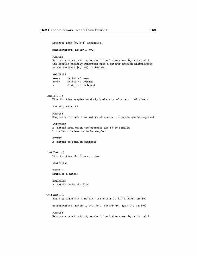
16.2 Random Numbers and Distributions 169
integers from [0, n-1] inclusive.
randint(nrows, ncols=1, n=2)
PURPOSE
Returns a matrix with typecode ’i’ and size nrows by ncols, with
its entries randomly generated from a integer uniform distribution
on the interval [0, n-1] inclusive.
ARGUMENTS
nrows number of rows
ncols number of columns
n distribution bound
sample(...)
This function samples randomly k elements of a vector of size n.
B = samples(A, k)
PURPOSE
Samples k elements from matrix of size n. Elements can be repeated.
ARGUMENTS
A matrix from which the elements are to be sampled
k number of elements to be sampled
OUTPUT
B matrix of sampled elements
shuffle(...)
This function shuffles a vector.
shuffle(A)
PURPOSE
Shuffles a matrix.
ARGUMENTS
A matrix to be shuffled
uniform(...)
Randomly generates a matrix with uniformly distributed entries.
uniform(nrows, ncols=1, a=0, b=1, method=’D’, gen=’D’, cuda=0)
PURPOSE
Returns a matrix with typecode ’d’ and size nrows by ncols, with

170 16 Extension gsl
its entries randomly generated from a uniform distribution on the
interval (a, b).
ARGUMENTS
nrows number of rows
ncols number of columns
a lower bound
b upper bound
CUDA methods:
method ordering method:
’D’ default ordering
’B’ best ordering
’S’ seeded ordering
CUDA generators:
gen random number generator:
’D’ pseudo default
’X’ pseudo xorwow
’Q’ quasi default
’S’ quasi Sobol32
’C’ quasi scrambled Sobol32
’A’ quasi Sobol64
’B’ quasi scrambled Sobol64
cuda enable or disable CUDA random number generator
unirand(...)
Randomly generates a number with uniformly distributed entries.
unirandom(a=0, b=1, method=’D’, gen=’D’, cuda=0)
PURPOSE
Returns a number generated from a uniform distribution on the
interval (a, b).
ARGUMENTS
a lower bound
b upper bound
CUDA methods:
method ordering method:
’D’ default ordering
’B’ best ordering
’S’ seeded ordering
CUDA generators:
gen random number generator:
’D’ pseudo default

16.2 Random Numbers and Distributions 171
’X’ pseudo xorwow
’Q’ quasi default
’S’ quasi Sobol32
’C’ quasi scrambled Sobol32
’A’ quasi Sobol64
’B’ quasi scrambled Sobol64
unisort(...)
Randomly generates a matrix with uniformly distributed entries
sorted in ascending order.
uniform(nrows, ncols=1, a=0, b=1, method=’D’, gen=’D’, cuda=0)
PURPOSE
Returns a matrix with typecode ’d’ and size nrows by ncols, with
its entries randomly generated from a uniform distribution on the
interval (a, b) sorted in ascending order.
ARGUMENTS
nrows number of rows
ncols number of columns
a lower bound
b upper bound
CUDA methods:
method ordering method:
’D’ default ordering
’B’ best ordering
’S’ seeded ordering
CUDA generators:
gen random number generator:
’D’ pseudo default
’X’ pseudo xorwow
’Q’ quasi default
’S’ quasi Sobol32
’C’ quasi scrambled Sobol32
’A’ quasi Sobol64
’B’ quasi scrambled Sobol64
cuda enable or disable CUDA random number generator
weibull(...)
This function returns a random variate from the Weibull distribution.
weibull(nrows, ncols=1, a=1, b=1)
PURPOSE

172 16 Extension gsl
Returns a matrix with typecode ’d’ and size nrows by ncols, with
its entries randomly generated from a Weibull distribution with
scale factor a and shape factor b.
ARGUMENTS
nrows number of rows
ncols number of columns
a scale factor
b shape factor
weibullcdf(...)
Weibull cdf.
weibullcdf(x)
PURPOSE
Returns the weibull cdf with scale parameter ’a’ and
shape parameter ’b’ of a real value x, as follows:
weibull(x) = 1 - exp((x/a)^b)
ARGUMENTS
a > 0 double scalar or matrix
b > 0 double scalar or matrix
x double scalar or matrix

Chapter 17
Device Classes and Methods
This chapter describes the main parameters, methods and sub-classes that composetypical devices. The chapter is organised as follows. Section 17.1 provides a listof the most important low-level classes on which all other devices are based. Sec-tion 17.2 describes the basic sub-classes that are often used in high-level devices.These include the classes to define variables and connections. Sections 17.3 and17.4 describe the main attributes that specifies the behaviour and the propertiesthat has to be defined in the init function of a device. Section 17.5 describesthe most common methods that have to be defined to set up a standard device.Section 17.6 describes other less common methods. Section 17.7 describes throughexamples methods and functions that simplifies the definition of some commonnonlinearities, such as anti-windup limiters and dead bands. Section 17.8 describesthe methods required to define delayed DAEs. Section 17.9 describes the methodsrequired to define stochastic DAEs. Finally, Section 17.10 describes how add per-manently a new device to Dome.
Note – Dome uses a vectorised approach to define devices. This means thatthe instance of a given device class is unique. Such an instance can have severalelements, i.e., as many as the declarations of such device in the data file. Internally,device parameters and indexes are organised as arrays and lists. All operationsimplemented in the methods of the device must be run for all elements of arraysand lists.
Note – The information provided in this chapter is intended only as a verybasic reference guide. Each device is a world apart and its implementation is one ofa kind. The best approach to implement a new model is to start with the workingcode of a device with similar characteristics and then customise such a code.
17.1 Low-Level Ancestors
The following is the list of principal ancestors of Dome devices. All classes beloware included in the folder dome.devices.
173

174 17 Device Classes and Methods
.device.core This class is common to all Dome devices including the classes inthe remainder of this list. It includes the definition of basic attributes, lowlevel methods and some void prototypes of high level methods. core per setakes care of the interaction of devices with the system but does not defineequations or any specific action. Very few devices require to inherit directlyfrom core. For example, all meta-devices (see Chapter 9).
.device.device This class is same as core and, additionally, defines the ac voltageand power bases, Vn and Sn, respectively. The class device is used for basicac devices and is the ancestor of the classes onebus, depark, and series
below.
.device.onebus This class is same as device but defines one ac bus connection ispolar coordinates using the class conn, as follows:
self. conn.set(’bus’, ’bus id’, (’a’, ’v’), ’Bus’)
where a and v are the indexes of bus voltage phase angles and magnitudes,respectively.
.device.depark This class is same as device but defines one ac bus connection isrectangular (dq-frame) coordinates using the class conn, as follows:
self. conn.set(’bus’, ’bus id’, (’vd’, ’vq’), ’PBus’)
where vd and vq are the indexes of bus voltage d and q components, respec-tively. This device also defines the attribute park as True.
.series.series.series This class defines low level methods and parameters ofac series devices based on standard phasor model. For example, it is theancestor of Line and Coupling. It assumes that devices are connected to twoac buses, as follows:
self._conn.set(’bus1’, ’sending-end bus id’, (’afr’, ’vfr’), \
’Bus’, (’a’, ’v’))
self._conn.set(’bus2’, ’receiving-end bus id’, (’ato’, ’vto’), \
’Bus’, (’a’, ’v’))
A void prototype of the method get flows is also defined here. Each seriesdevice will have to overwrite this function that returns the sending-end andreceiving-end injected complex powers. The prototype of this function definedin series is as follows:
def get_flows(self, dae, idx, Vs, Vr):

17.2 Basic Sub-classes 175
"""This method must be overwritten by children classes"""
if not len(idx): idx = list(range(self.n))
S = self.u[idx] + 0j
return S, S
where Vs and Vr are the complex voltages at the sending and receiving-end,respectively.
.series.park.pseries This class is based on series and defines low level meth-ods and parameters of ac series devices based on the dq-frame model. Forexample, it is the ancestor of PLine and PCoupling. It assumes that devicesare connected to two ac buses, as follows:
self._conn.set(’bus1’, ’sending-end bus id’, (’vd1’, ’vq1’), \
’PBus’, (’vd’, ’vq’))
self._conn.set(’bus2’, ’receiving-end bus id’, (’vd2’, ’vq2’), \
’PBus’, (’vd’, ’vq’))
All other methods and parameters are inherited from series.
.load.common.pfload This class provides a common set of methods for ac loads.It is used as ancestor for most loads included in the folder device.load.Another class, .load.common.utils provides extra useful methods for load.The class .load.common.baseload conveniently puts together pfload andutils. Refer to the source code for details.
.emt.basic.common This is the base class for high-voltage EMT dipoles. All circuitdevices such as R, RL, etc., are defined based on this class. Refer to the sourcecode for details. Dipoles are connected to two Node’s, as follows.
self._conn.set(’node1’, ’1st node id’, (’v1’, ), ’Node’, (’v’, ))
self._conn.set(’node2’, ’2nd node id’, (’v2’, ), ’Node’, (’v’, ))
.electronic.basic.common This is the base class for low-voltage EMT dipoles.All circuit devices such as ER, ERL, etc., are defined based on this class. Referto the source code for details. Dipoles are connected to two Pin’s, as follows.
self._conn.set(’pin1’, ’1st pin id’, (’v1’, ), ’Pin’, (’v’, ))
self._conn.set(’pin2’, ’2nd pin id’, (’v2’, ), ’Pin’, (’v’, ))
17.2 Basic Sub-classes
Dome exploits the ability of Python to define and embed classes and subclass toachieve and high degree of code flexibility and modularity. With this aim, thedefinition of variables and connections of devices is not handled by the device itselfbut through sub-classes which can be customised to cope with complex task. Theseclasses are described in the remainder of the section.

176 17 Device Classes and Methods
17.2.1 Variables
The class variable is defined in the module dome.devices.device. Currently, itis utilised to define state, algebraic and switching-manifold variables, as follows:
self._state = variable(self, ’_state’, ’state variables’)
self._algeb = variable(self, ’_algeb’, ’algebraic variables’)
self._switch = variable(self, ’_switch’, ’switching manifolds’)
The line above are included in the init method of the class core, and thus makeavailable state, algebraic and switching-manifold variables to all Dome devices.However, once instantiated, state, algeb, and switch are void.
To define a variable within a device, one has to include in the init methodof such a device a call to the set method of the variable that has to be added. Forexample:
self._state.set(’delta’, r’\delta’, ’rotor angle’, ’rad’)
self._state.set(’omega’, r’\omega’, ’rotor angular speed’, ’pu(Hz)’, ’M’)
where the first argument is the name of the indexes of the variable the will be usedin the device; the second argument is the LATEX name of the variable used for plot-ting; the third argument is a short description of the variable; the fourth argumentis the variable unit; and the fifth argument is the time constant of the variable.The fifth argument is optional for state variables and unnecessary for algebraicand switching manifold variables. Also the unit is optional. If not provided, theunit will be assume to be ’-’. Once the variables delta and omega are defined asabove, the other methods of the device will be able to access the indexes of suchvariables through the attributes self.delta and self.omega. These indexes referto the positions of such variables in the corresponding array of the DAE system.State variables are included in the array system.DAE.x;1 algebraic variables areincluded in the array system.DAE.y. Note, however, that switching manifolds donot introduce new variables. The indexes can be also used to access the value ofthe equations corresponding to such variables, as follows. Differential equationsare included in the array system.DAE.f; algebraic equations are included in thearray system.DAE.g; and switching manifold equations are included in the arraysystem.DAE.s.
Hot Tip – It is important to remember that the indexing of differential andalgebraic equations is somewhat arbitrary. It is up to the user to associate in ameaningful way the indexes of state and algebraic variables to the positions of thedifferential and algebraic equations. For example, it makes sense that the differen-tial equation that defines δ is indexed with self.delta.
Most of the other methods and functionalities of the class variable are usedin the low level methods of the class core and are not needed, in general, whendefining new devices. The following are a few methods that can be useful in somecases.
1Note that, in general, system.DAE is passed to the device methods as an argument of themethod itself and, conventionally, it is called dae.

17.2 Basic Sub-classes 177
update(...) Allows updating the parameters of an existing variable. This can beuseful, for example, if a new device is based on an existing one but needs toredefine some variables. The syntax of the method is:
self._state.update(var, doc=None, uni=None, tmc=None)
where var is the name of the variable to update and the other fields are thedescription (doc), the units (uni), and the time constant (tmc).
remove(...) Removes an existing variable. This can be useful, for example, if anew device is based on an existing one but does not share the same variables.The syntax of the method is:
self._state.remove(var)
where var is the name of the variable to be removed (same string as the firstargument of the method set)
vars() Returns an iterator on the defined variables. The syntax of the method is:
self._state.vars()
This method has to be used within a for- or a while-loop.
17.2.2 Connections
The class connection is defined in the module dome.devices.device. Currently,it is utilised to define any kind of physical connection to topological devices, suchas Bus, PBus, Node, and Pin. The class is instantiated as follows:
self._conn = connection(self)
The line above are included in the init method of the class core, and thus makeavailable topological connections to all Dome devices. However, once instantiated,the attribute conn is void.
To define a connection within a device, one has to include in the init methodof such a device a call to the set method of the variable that has to be added. Forexample:
self._conn.set(’bus’, ’Bus id’, (’a1’, ’v1’), ’Bus’, (’a’, ’v’))
where the first argument is the name of the indexes of the topological element thatwill have to be defined in the data file; the second argument a short descriptionof the connection; the third argument is a tuple of string that will be used in thedevice to refer to the connection variable indexes; the fourth argument is the nameof the topological device to be connected to; and the fifth argument is a tuple of thenames of variable indexes as defined in the topological device. The fifth argumentis optional if it is the same as the tuple provided as third argument. Once the con-nection is defined, the other methods of the device will be able to access the indexes

178 17 Device Classes and Methods
of such variables through the attributes self.a1 and self.v1. These indexes referto the positions of such variables in the corresponding algebraic variable array ofthe DAE system, i.e., system.DAE.y.
The same indexes also refer to the position within the vector of algebraic equa-tions that define power/current balances. In this example, self.a1 and self.v1
are the indexes of the active and reactive power balances, respectively, in the vectorsystem.DAE.g.
The following is the list of connections and balance equations:
Bus a and v are the indexes of bus voltage phase angles and magnitudes in thevector system.DAE.y, respectively, as well as, the indexes of the active andreactive power balances, respectively, in the vector system.DAE.g.
PBus vd and vq are the indexes of bus voltage d- and q-axis components in thevector system.DAE.y, respectively, as well as, the indexes of the d- and q-axiscurrent injection balances, respectively, in the vector system.DAE.g.
Node v are the indexes of node voltage magnitudes in the vector system.DAE.y, aswell as the indexes of the current injection balances in the vector system.DAE.g.
Pin v are the indexes of node voltage magnitudes in the vector system.DAE.y, aswell as the indexes of the current injection balances in the vector system.DAE.g.
Most of the other methods and functionalities of the class connection are usedin the low level methods of the class core and are not needed, in general, whendefining new devices. The following method that can be useful in some cases.
remove(...) Removes an existing variable. This can be useful, for example, if anew device is based on an existing one but does not share the same variables.The syntax of the method is:
self._conn.remove(name)
where name is the name of the connection to be removed (same string as thefirst argument of the method set).
17.3 Attributes
This section describes the meaning and purpose of the attributes that are set upwhenever instantiating a new device. These attributes are generally assigned in themethod init . Attributes are organised into two groups: (i) device attributes;and (ii) data attributes.

17.3 Attributes 179
17.3.1 Device Attributes
Attributes that are common to all devices are described below.
self.n is an integer indicating the number of elements of the device. By defaultthis number is zero. self.n is incremented by one for every definition of thedevice in the data file. self.n is the size of every array of the parametersand list of indexes of the device and can thus be used to iterate over suchattributes.
self.u indicates the connection status of the device. It is a dense real matrix ofsize self.n. An element i of the device is on-line or enabled if self.u[i] is1; an element i of the device is off-line or disabled if self.u[i] is 0.
self.name indicates the names of each element of the device. It is a list of stringsof size self.n. The names of the list does not need to be unique.
self.int indicates the IDs of each element of the device. It is a dictionary ofsize self.n where the keys are the IDs and the values are the number of theelements (in the same order they where defined in the data file), starting from0. The keys of the dictionary must be unique.
self.idx indicates the IDs of each element of the device. It is a list of size self.nwhere the elements are the IDs and the positions of such elements are thenumber of the elements (in the same order they where defined in the datafile), starting from 0. The elements of self.idx are the ordered keys ofself.int.
self.system is a pointer to the whole system. It allows each device to access atany time any other attribute and method of the system and thus of any otherdevice. This attribute is use to grab data from other devices or system settingswithout the need to pass explicitly as arguments such data and settings.2
self. group is a string indicating the group to which the device belongs. It hasto be one of the keys of the dictionary system.device groups.
self. category is a tuple of strings indicating the categories to which the devicebelongs. Each element of the tuple has to be one of the keys of the dictionarysystem.device categories.
self. name is a string that contains the name of the device, e.g., Bus, Line, Syn6a.Device names are typically upper case. This string is used to instantiatethe device class in the overall class system, e.g., system.Bus, system.Line,system.Syn6a.
self. conn is an instance of the class connection. See subsection 17.2.2.
2This attribute has to be used with caution as it might compromise the purity of functions andmethods of the device. A pure function is a function that always returns the same outputs giventhe same inputs. A pure function is said not to have side effects. A discussion on side effects canbe found at https://en.wikipedia.org/wiki/Side_effect_(computer_science).

180 17 Device Classes and Methods
self. state is an instance of the class variable and is used to handle state vari-ables. See subsection 17.2.1.
self. algeb is an instance of the class variable and is used to handle algebraicvariables. See subsection 17.2.1.
self. switch is an instance of the class variable and is used to handle switchingmanifold variables. See subsection 17.2.1.
self. nseries indicates the starting index of the device if this is a series device(see also the property series in Section 17.4) This is generally set up by theclass series (see Section 17.1). Default value is None.
self. hidden if True, the device is hidden and cannot be set by the user. Anexample of hidden device is COI, that calculates the frequency of the centreof inertia of the system. This device is enabled if Settings.coi is True butcannot be accessed directly by the user.
self. links is a list of (name, idx) pairs of the devices to which the device isconnected. This is generally handled by the self. conn class and by themethod set links.
self. avatar is a Boolean. If True, the device can be removed after the power flowanalysis. This attribute is used only by the routine that calculates reduced-size equivalent networks.
self. park is a Boolean. If True, the Park’s vector is used for interface equations.
self. broken is a Boolean. If True, the device is incomplete or equations containerrors. Only used for development.
self. deprecated is a Boolean. If True, the device is obsolete or superseded by anew one. For example, device Syn5a is deprecated and should be substitutedfor Syn6a with Td20 = 0 and xq2 = xd2 = xd1.
self. ac is a Boolean. It is True if the device includes ac quantities and its ownac nominal quantities.
self. dc is a Boolean. It is True if the device includes dc quantities and its ownac nominal quantities.
self. fc is a Boolean. It is True if the device defines its local frequency base.
self. auxiliary contains the names of quantities and constants that are auxil-iary, i.e., are defined internally by the device (typically within the methodsself.xinit and setx0). To include the names of auxiliary quantities andconstants is not strictly required, but it is highly recommended to improvethe consistency of the code.
self. VBac is a dense real array or size self.n. It contains the local ac voltagebases for each device element.

17.3 Attributes 181
self. SBac is a dense real array or size self.n. It contains the local ac apparentpower bases for each device element.
self. VBdc is a dense real array or size self.n. It contains the local dc voltagebases for each device element.
self. IBdc is a dense real array or size self.n. It contains the local dc currentbases for each device element.
17.3.2 Data Attributes
The parameters that can be defined in the data file for each device are handledthrough a dictionary, called data and a set of other attributes that define thebehaviour of each parameter. The main attributes to define data are describedbelow.
self. data is a dictionary whose keys are the names of the parameters and asso-ciated values are the default values of each parameter. Such default valuesare used if the user does not define a parameter in the data file. u is alwaysa key of self. data and by default is 1. For example:
self._data = ’M’:5.0, ’xd1’:2.0, ’D’:0, ’gen’:None, ’u’:1
Once initialised, the device will have the following attributes:
self.M
self.xd1
self.D
self.gen
self.u
In the data file the user can define:
SynEleMec, M=5.34, D=0.1, gen=’gen 1’
Since they are not defined, xd1 and u will be assigned the default values 2.0and 1.
self. params is a list whose elements are the names of the parameters (i.e., thekeys of the dictionary self. data) that have to be converted to dense realmatrices. Keys that are not included in self. params will be Python lists.For example:
self._params = [’u’, ’key1’, ’key2’]
will make the attributes u, self.key1 and self.key3 as dense real matrices.On the other hand, self.key3 of the example above will be a list of strings.self. params is initialised as [’u’, ].

182 17 Device Classes and Methods
self. data unit is a dictionary where the keys are the same keys as the dictionarydata and the values are the units of each key. Per unit values should alsoindicate the absolute units, e.g., pu(kV), pu(MW) and pu(MVAr). self. unit
is initialised as ’u’:’bool’.
self. data doc is a dictionary where the keys are the same keys as the dictionarydata and the values are a brief description of each key. The description canbe an empty string. self. doc is initialised as ’u’:’connection status’.
The utility function self.set datum(...) simplifies the definition of new pa-rameters. The syntax is as follows:
self.set_datum(prop, val, doc, unit=’-’, param=True)
where prop is a string that identifies the name of the new parameter, val is thedefault value, doc is a brief description, unit is the unit of the parameters, andparam is True if the attribute has to be converted to a dense real matrix, and False
is the attribute has to be converted to a Python list. For example:
self.set_datum(’M’, 5, ’inertia constant’, ’kWs/kVA’)
self.set_datum(’xd1’, 2, ’transient reactance’, ’pu(Ohm)’)
Note that the method self.set datum simply populates the dictionaries and listsself. data, self. doc, self. unit, and self. params, so its use is not manda-tory. However, it is highly recommended to utilise such a function to make surethat each data is properly and safely set up.3
The following are optional attributes that can be defined for each data. Allattributes below are Python lists whose elements can be exclusively the keys of thedictionary self. data. By default, the lists below are empty.
self. powers contains the names of the parameters that are powers, energies,inertias and dampings.
self. voltages contains the names of the parameters that are ac voltages.
self. currents contains the names of the parameters that are ac currents.
self. z contains the names of the parameters that are impedances.
self. y contains the names of the parameters that are admittances.
self. dccurrents contains the names of the parameters that are dc currents (forEMT circuits).
self. dcvoltages contains the names of the parameters that are dc voltages (forEMT circuits).
3The function self.set datum, in fact, is guaranteed to work also for future version of Dome,where the attributes self. data, self. data doc, self. data unit, and self. params can havedifferent names or purposes.

17.4 Properties 183
self. r contains the names of the parameters that are resistances (for EMT cir-cuits).
self. g contains the names of the parameters that are susceptances (for EMTcircuits).
self. zeros contains the names of the parameters whose value cannot be zero.
self. times contains the names of the parameters that are time constants.
self. mandatory contains the names of the parameters that are mandatory, i.e.,must be defined in the data file.
The following are some examples of usage of non-mandatory data attributes:
self.set_list(’_zeros’, ’M’)
self.set_list(’_powers’, ’D’, ’M’)
self.set_list(’_z’, ’xd1’)
self.set_list(’_auxiliary’, ’e’, ’pm’)
self.set_list(’_mandatory’, ’bus’, ’gen’)
Note the use of the utility function self.set list which safely populates the lists.
17.4 Properties
Every device includes a dictionary called properties whose keys specifies the be-haviour of the device and the methods that can be called. By default, all valuesassociated to the keys of the properties dictionary are initialised as False. Thus,one has to indicate only those properties that are True. The remainder of thissection describes the meaning and purpose of each property.
ecall call the differential and algebraic equations. It implies that the device in-cludes a method ecall.
ejacs call the time-variant Jacobians of differential and algebraic equations. Itimplies that the device includes the methods ejacs and getidx.
cjacs call the constant Jacobians of differential and algebraic equations. It impliesthat the device includes the methods cjacs and getidx.
mjacs call the Jacobians of differential and algebraic equations with respect to thecontinuation parameter µ. It implies that the device includes the methodsmjacs and getidx mu. This property has effect only for the continuationpower flow analysis.
switch call the switching manifold equations and Jacobians of switching manifoldequations. It implies that the device includes the methods scall, sjacs, andgetidx sw. This property is still beta and has effect only for the time domainanalysis and the option TDS.switching is True.

184 17 Device Classes and Methods
windup call the function for anti-windup limiters. It implies that the device in-cludes the method windup. This property has effect only for the time domainanalysis.
pflow if True, the device is called during the power flow analysis, otherwise, de-vice’s DAEs are initialised after the solution of the power flow analysis.
xinit call the initialisation of device DAEs and parameters. If pflow is True, thedevice must include the method xfirst. If pflow is False, the device mustinclude the method setx0.
shunt this property indicates that the device is a shunt, i.e., it is connected toa single ac bus and consumes power. It has effects when Dome creates thepower flow report, loss calculations, and system statistics. This property isenabled by the class baseload.
series this property indicates that the device is a series, i.e., it is connected totwo ac buses. It has effects when Dome creates the power flow report, losscalculations, and system statistics. This property is enabled by the classseries.
flows this property indicates that the device defines a method to compute injectedpowers at sending and receiving ends. It implies that device includes themethod flows. It has effects when Dome creates the power flow report,loss calculations, and system statistics. This property is enabled by the classseries.
connection this property indicates that the device is a topological node. It haseffects only for system statistics. This property is enabled by the devices Bus,PBus, Node, and Pin.
times this property indicates that the device defines events at fixed times. If True,the device must include the method get times. It has effects only for timedomain analysis.
stagen this property indicates that the device is a static generators (e.g., PVgen).It has effects for power flow report, initialisation of dynamic generators andsystem statistics.
dyngen this property indicates that the device is a static generators (e.g., syn-chronous machines). It has effects for power flow report, initialisation ofdynamic generators and system statistics.
dcseries this property indicates that the device is a series, i.e., it is connected totwo Node’s or Pin’s. It has effects when Dome creates the power flow reportand system statistics. All high-voltage EMT devices connected to at leasttwo Node’s have this property equal to True.

17.5 Common Methods 185
opf this property indicates that the device is used for optimal power flow anal-ysis. If True, it implies that the devices includes a set of methods, as fol-lows: setup opf ecall opf, getidx opf, ejacs opf, guess opf, opfrep,ehess opf, ocall, ojacs. This property is enforced by the class devopf thatis part of the module devices.device and has to be included in the preambleof a device class aside the main device ancestor discussed in Section 17.1.
delay this property indicates that the device defines delayed DAEs. It has effectonly for time domain and small-signal stability analyses. If True, the devicemust include the methods get delay and djacs.
stochastic this property indicates that the device defines stochastic DAEs. Ithas effect only for time domain. If True, the device must include the methodwcall. This property is generally enabled by including in the preamble of thedevice a class that defines a stochastic process, for example, wiener that isdefined in the module devices.math.stochastic.
reinit this property indicates that the device defines a re-initialisation functionfor state variables. It has effect only for time domain analysis. If True, thedevice must include the method reinit. See the source code of the devicedevices.math.physical.bounchingball.
post this property indicates that the device requires some calculations after thesolution of each step of the time domain analysis. If True, the device mustinclude the method post tds. Most devices that include stochastic processesrequires to enable this property.
The following are some examples of usage of the property dictionary:
self.set_dict(’properties’,
dyngen = True,
ejacs = True,
xinit = True,
ecall = True,
cjacs = True)
Note the use of the utility function self.set dict which safely populates thedictionary.
17.5 Common Methods
This section describes the most common methods that are needed to define thestructure and the mathematical model of most devices included in Dome.4
init initialises the device including data and properties as described in Sections17.3 and 17.4.
4Special devices such as, for example, meta-devices, are not covered in this and followingsections are they often require ad hoc functions or redefine low level methods defined in the basicclasses described in Section 17.1.

186 17 Device Classes and Methods
xfirst defines initial guesses for state and algebraic variables and initialises aux-iliary constants and parameters. This method is called only if the propertiespflow and xinit are True.
setx0 initialises state and algebraic variables as well as auxiliary constants andparameters. This method is called only if the properties pflow is False andxinit is True.
ecall calls differential and algebraic equations. This method is called only if theproperty ecall is True.
dynidx defines the indexes of state and algebraic variables in the DAE vectors.The method is predefined in the core device classes but can be overwritten inthose cases where state and algebraic variables are not known a priori, e.g.,for those devices whose order depends on user input data.
getidx defines the nonzero elements of the system Jacobian matrices. This methodis called if either property cjacs or ejacs is True. The attributes of the inputargument dae that includes the lists of nonzero elements are as follows:
igy, jgy row and column indexes of the matrix ∂g/∂y.
igx, jgx row and column indexes of the matrix ∂g/∂x.
ify, jfy row and column indexes of the matrix ∂f/∂y.
ifx, jfx row and column indexes of the matrix ∂f/∂x.
itx, jtx row and column indexes of the matrix T x.
irx, jrx row and column indexes of the matrix Rx.
The following are relevant remarks:
• Elements that are common in (itx, jtx) and (ifx, jfx) can be definedonly in (itx, jtx).
• Elements that are common in (irx, jrx) and (igx, jgx) can be definedonly in (irx, jrx).
• Diagonal elements in (itx, jtx), (ifx, jfx) and (igy, jgy) do not needto be defined.
• Repeated indexes are allowed but should be avoided.
cjacs calls the constant Jacobian matrices of differential and algebraic equations.This method is called only if the property cjacs is True.
ejacs calls the time-variant Jacobian matrices of differential and algebraic equa-tions. This method is called only if the property ejacs is True.
tcall defines diagonal elements of matrix T x using the information provided inthe definition of self. state.set(...) method. This function does notgenerally need to be overwritten. Note that tcall is called after the methodsetx0 and, hence, time constants can be defined on-the-fly.

17.5 Common Methods 187
custom is an optional method that, if defined, perform any required operation afterthe power flow analysis. It can be useful whenever one needs to solve someoperations that requires the knowledge of the power flow solution and has tobe performed before any other routine starts.
Examples of most methods described above can be found in Chapters 2 and 10 andAppendix C. Figure 17.1 shows the order with which the device methods are calledduring the execution of Dome. Methods outside the power flow analysis loop arecalled only once.
17.5.1 Time-variant Matrices T x and Rx
As discussed in Subsection 2.5.1 of Chapter 2, matrices T x and Rx do not haveto be constant. In this case, one needs to access the time derivatives of the statevariables. Due to the semi-implicit notation, such time derivatives are available,during the time domain integration, as a numerical approximation in the arraydae.d.
Let’s consider the following differential equation:
T · y · x = f(x)
where y is a variable. Then, the time constant if T · y and is not constant. Theelements of the Jacobian matrix can be accounted for in the method ejacs, asfollows:
def ejacs(self, dae):
sdassign(dae.Tx, mul(self.T, dae.y[self.y]), self.x)
spassign(dae.Ty, mul(self.T, dae.d[self.x]), self.x, self.y, self.u)
where self.T is the array of time constants T ; self.x and self.y are the indexesof the state variable x and the algebraic varaible y, respectively; and self.d is thenumerical approximation of x. Note that the matrix dae.Ty needs to be initializedwith the method getidx:
def getidx(self, dae):
dae.ity += self.x
dae.jty += self.y
The use of the functions sdassign and/or spassign is mandatory for the timeconstant matrices, as these are not re-initialized at every iteration. Note that, asfor any other Jacobian matrix, diagonal elements of T x do not need to be definedin getidx.
Similarly, time-variant elements of the matrix Rx can be accounted for by prop-erly assigning the elements of dae.Rx, and dae.Ry; and by initializing non-zeroelements with dae.irx and dae.jrx for dae.Rx, and dae.iry and dae.jry fordae.Ry.

188 17 Device Classes and Methods
dynidx
xfirst
getidx
Power Flow Analysis
ecall
cjacs
ejacs
dynidx
setx0
custom
Post Power Flow Operations
Pre Power Flow Operations
Exit or Run Other Routine
Loop
getidx
tcall
init
Figure 17.1: Sequence of calls to device methods during the execution of the powerflow analysis.
17.6 Less Common Methods
This section describes the less common methods that are needed to define thestructure and the mathematical model of some devices included in Dome.

17.6 Less Common Methods 189
17.6.1 Methods for Discrete Events
Discrete events are handled in Dome through mainly two methods, event andget times, which have effect only during time domain simulations. The eventshandled by these functions happens at times known a priori. State driven eventscan be handled using switching manifolds.
event applies an event. This function is triggered by a fixed time defined in themethod get times below.
get times returns a list of times at which the vents occurs. It is often useful toreturn also a list of times that are slightly before the events, so that plottingtrajectories will clearly show the time at which the event has occurred. Thismethod is called only if the property times is True.
For example, let’s consider the case of induction motor start-ups. These areevents that happens at the times indicated in the parameter tup and a triggered ifthe elements of the parameter startup are True.
def get_times(self):
if not self.n: return []
tup = self.tup[:]
for item in range(self.n - 1, -1, -1):
if not self.startup[item] and not self.u[item]: tup.pop(item)
tup = set(tup)
tup = tup.union(tup)
u = matrix(list(tup))
return list(u - 1e-6) + list(u)
def event(self, dae):
# define start-up conditions
update = startup(self.sup, dae.t, self.tup, self.u, self.name)
if update: self.system.DAE.factorize = True
17.6.2 Methods for Switching Manifolds
Switching manifolds allow determining exactly the occurrence of a state-drivenevent. For example, the time at which a certain state variable reaches its maximumor minimum value. With this aim, one needs to define three functions, getidx sw,scall and sjacs. These function are enabled if the device property switch andthe time domain integration option TDS.switching are True.
getidx sw the indexes of the nonzero elements within the Jacobian matrices of theequations of the switching manifolds.

190 17 Device Classes and Methods
isy, jsy row and column indexes of the matrix ∂s/∂y.
isx, jsx row and column indexes of the matrix ∂s/∂x.
scall calls the switching manifold equations.
sjacs calls the Jacobian matrices of the switching manifold equations.
For example, let’s assume that an AVR includes a limiter on the output regulatorvoltage. The first step is to add to the method init the variables for theswitching manifolds:
self._switch.set(’vrmax’, r’v_r \max’,
’maximum regulator voltage’, ’pu(kV)’)
self._switch.set(’vrmin’, r’v_r \min’,
’minimum regulator voltage’, ’pu(kV)’)
Assuming that the output regulator voltage is indexed through the attribute self.vr2,the three methods above becomes:
def getidx_sw(self, dae):
dae.isx += self.vrmax + self.vrmin
dae.jsx += 2 * self.vr2
def scall(self, dae):
vr2 = dae.x[self.vr2]
mupdate(dae.s, self.rmax - vr2, self.vrmax, self.u)
mupdate(dae.s, vr2 - self.rmin, self.vrmin, self.u)
def sjacs(self, dae):
spupdate(dae.Sx,-1, self.vrmax, self.vr2, self.u)
spupdate(dae.Sx, 1, self.vrmin, self.vr2, self.u)
17.6.3 Sequence of Calls for Time Domain Simulations
Figure 17.2 shows the order with which the device methods are called during theexecution of Dome. Methods outside the time domain simulation loop are calledonly once. The “root solving” section is exectured only is the option TDS.switching
is True.
17.6.4 Methods for Continuation Power Flow Analysis
The continuation variable is assumed to be a factor that multiplies the active powerconsumption (or production) of loads (or generators). Such variable is called mu
and is an attribute of system.DAE (or dae, when passed as an argument to device

17.6 Less Common Methods 191
get times
getidx sw
Time Domain Simulation
event
cjacs
ejacs
wcall
windup
post tds
Pre TDS Operations
Exit or Run Other Routine
Loop
scall
Update Time
ecall
Solve Time Step
Loop
sjacs
scall
Root Solving
Figure 17.2: Sequence of calls to device methods during the execution of the timedomain simulations.
methods). There are two function specific for the continuation variable, getidx mu
and mjacs. These functions are enabled if the property mjacs is True. Note thatthere is no mcall method because the continuation variable is accounted for inthe method ecall. The continuation variable dae.mu is equal to 1 except for thecontinuation power flow analysis.
getidx mu the indexes of the nonzero elements within the Jacobian matrices of theequations of the switching manifolds.
igm row indexes of the matrix ∂g/∂µ.
ifm row indexes of the matrix ∂f/∂µ.

192 17 Device Classes and Methods
Note that there are no fields jgm and jfm because µ is scalar.
mjacs calls the Jacobian matrices of the switching manifold equations.
For example, let’s consider the case of voltage dependent load whose powerconsumption is described by the following equation:
p = µp0vap
q = µq0vaq
Then the methods ecall, getidx mu and mjacs would look like the following:
def ecall(self, dae):
v = dae.y[self.v]
mupdate(dae.g, dae.mu*mul(self.p0, mpow(v, self.ap)), self.a)
mupdate(dae.g, dae.mu*mul(self.q0, mpow(v, self.aq)), self.v)
def getidx_mu(self, dae):
dae.igm += self.a + self.v
def mjacs(self, dae):
v = dae.y[self.v]
spupdate(dae.Gm, mul(self.p0, mpow(v, self.ap)), self.a, 0)
spupdate(dae.Gm, mul(self.q0, mpow(v, self.aq)), self.v, 0)
where self.a and self.v are the indexes of the active and reactive power injectionsof the load (see also Section 12.1).
17.6.5 Methods for Optimal Power Flow Analysis
We illustrate the functions required for the Optimal Power Flow (OPF) analysisthrough a simple but rather complete example. This implements a model of asupply bid, which defines a quadratic objective function and limits its power bids.The code of this model is as follows.
class basebid(onebus, devopf):
def __init__(self, system, name):
super(basebid, self).__init__(system, name)
self._group = ’Market’
self._category = ’Transmission’,

17.6 Less Common Methods 193
self._init_opf()
self._yopf.set(’p’, r’p’, ’active power supply’, ’pu(MW)’)
self._copf.set(’px’, r’p_\max’, ’slack variable of active’ + \
’ power supply upper bound’, ’pu(MW)’)
self._copf.set(’pn’, r’p_\min’, ’slack variable of active’ + \
’ power supply lower bound’, ’pu(MW)’)
self.set_datum(’cp0’, 0.0, ’active power c0 bid’, ’$/h’)
self.set_datum(’cp1’, 0.0, ’active power c1 bid’, ’$/MWh’)
self.set_datum(’cp2’, 0.0, ’active power c2 bid’, ’$/MW^2h’)
self.set_datum(’cq0’, 0.0, ’reactive power c0 bid’, ’$/h’)
self.set_datum(’cq1’, 0.0, ’reactive power c1 bid’, ’$/MVArh’)
self.set_datum(’cq2’, 0.0, ’reactive power c2 bid’, ’$/MVAr^2h’)
self.set_datum(’pmax’, 0.0, ’maximum active power’, ’pu(MW)’)
self.set_datum(’pmin’, 0.0, ’minimum active power’, ’pu(MVAr)’)
self.set_datum(’tie’, 0.0, ’tie-break cost’, ’$/MWh’)
self.set_list(’_powers’, ’pmax’, ’pmin’)
def getidx_opf(self, dae):
dae.ihz += self.pn + self.px
dae.jhz += 2 * self.p
def ecall_opf(self, dae):
mupdate(dae.h, self.pmin - dae.y[self.p], self.pn)
mupdate(dae.h, dae.y[self.p] - self.pmax, self.px)
def ejacs_opf(self, dae):
spupdate(dae.Hz,-1.0, self.pn, self.p)
spupdate(dae.Hz, 1.0, self.px, self.p)
def guess_opf(self, dae):
self._guess_opf(dae, ’p’, ’pmax’, ’pmin’, ’px’, ’pn’)
mupdate(dae.rho, self.cp1, self.a)
mupdate(dae.rho, self.cq1, self.v)
class supply(basebid):
"""Supply bids"""
def __init__(self, system, name):
super(supply, self).__init__(system, name)

194 17 Device Classes and Methods
self._group = ’Market’
self._yopf.set(’q’, r’q’, ’reactive power supply’, ’pu(MVAr)’)
self._copf.set(’qx’, r’q_\max’, ’slack variable of ’ + \
’reactive power upper bound’, ’pu(MVAr)’)
self._copf.set(’qn’, r’q_\min’, ’slack variable of ’ +
’reactive power lower bound’, ’pu(MVAr)’)
self._opf[’Active Power Supply’] = [’pn’, ’pmin’, ’p’, ’pmax’, ’px’]
self._opf[’Reactive Power Supply’] = [’qn’, ’qmin’, ’q’, ’qmax’, ’qx’]
self.set_datum(’qmax’, 0.0, ’maximum reactive power’, ’pu(MVAr)’)
self.set_datum(’qmin’, 0.0, ’minimum reactive power’, ’pu(MVAr)’)
self.set_list(’_powers’, ’qmax’, ’qmin’)
def ecall_opf(self, dae):
super(supply, self).ecall_opf(dae)
mupdate(dae.g, -dae.y[self.p], self.a)
mupdate(dae.g, -dae.y[self.q], self.v)
mupdate(dae.h, self.qmin - dae.y[self.q], self.qn)
mupdate(dae.h, dae.y[self.q] - self.qmax, self.qx)
def getidx_opf(self, dae):
super(supply, self).getidx_opf(dae)
dae.igz += self.a + self.v
dae.jgz += self.p + self.q
dae.ihz += self.qn + self.qx
dae.jhz += 2 * self.q
dae.ioz += self.p + self.q
dae.ihe += self.p + self.q
dae.jhe += self.p + self.q
def ejacs_opf(self, dae):
super(supply, self).ejacs_opf(dae)
spupdate(dae.Gz,-1.0, self.a, self.p)
spupdate(dae.Gz,-1.0, self.v, self.q)
spupdate(dae.Hz,-1.0, self.qn, self.q)
spupdate(dae.Hz, 1.0, self.qx, self.q)

17.7 Methods for Common Nonlinearities 195
def ehess_opf(self, dae):
spupdate(dae.Hes, 2 * self.system.OPF.scaling * \
(self.cp2 + self.tie), self.p, self.p)
spupdate(dae.Hes, 2 * self.system.OPF.scaling * \
self.cq2, self.q, self.q)
def guess_opf(self, dae):
super(supply, self).guess_opf(dae)
self._guess_opf(dae, ’q’, ’qmax’, ’qmin’, ’qx’, ’qn’)
def ocall(self, dae):
p = dae.y[self.p]
q = dae.y[self.q]
dae.obj += sum(self.cp0) + sum(self.cq0)
dae.obj += dotu(self.cp1, p) + dotu(self.cq1, q)
dae.obj += dotu(self.cp2 + self.tie, p**2) + \
dotu(self.cq2, q**2)
def ojacs(self, dae):
spupdate(dae.Oz, self.cp1 + 2 * mul(self.cp2 \
+ self.tie, dae.y[self.p]), self.p, 0)
spupdate(dae.Oz, self.cq1 + 2 * mul(self.cq2, \
dae.y[self.q]), self.q, 0)
Note the attributes self. yopf and self. copf which are instances of the classvariable (see Subsection 17.2.1) and define OPF algebraic and slack variables,respectively.
17.7 Methods for Common Nonlinearities
This section describes some common nonlinearities that occurs in controllers. Theseare the windup limiter, the anti-windup limiter, the dead band, and the hysteresis.Most nonlinearities involve if-then rules. For efficiency, these are implemented inDome as Boolean variables, conventionally stating with a z. Such variables areassumed to be dense real matrices of length self.n.
17.7.1 Anti-windup Limiter
The anti-windup limiter locks both the state variables and its time derivative. Let’sassume that the differential equation:
T x = y − x

196 17 Device Classes and Methods
1
1+sT
y x
xmin
xmax
Figure 17.3: Lag transfer function with an anti-windup limiter.
undergoes an anti-windup limiter that bounds x to its limits xmax and xmin (seeFigure 17.3). The limiter equations are:
if x ≥ xmax and x ≥ 0 ⇒ x = xmax and x = 0
if x ≤ xmin and x ≤ 0 ⇒ x = xmin and x = 0
otherwise ⇒ T x = y − x
To set up an anti-windup limiter one needs to properly modify a few methods, asfollows.
def __init__(self, system, name):
super(dummydevice, self).__init__(system, name)
self.set_state(’x’, ’x’, ’bounded state variable’, ’-’, ’T’)
self.set_algeb(’y’, ’y’, ’input variable’, ’-’)
self.set_datum(’T’, 1, ’time constant’, ’s’)
self.set_datum(’xmax’, 1, ’max value of x’)
self.set_datum(’xmin’,-1, ’min value of x’)
self.set_dict(’properties’,
setx0 = True,
ecall = True,
cjacs = True,
windup = True,
)
self.set_list(’_auxiliary’, ’z’)
def setx0(self, dae):
self.z = matrix(self.u)
massign(dae.y, 0, self.x, self.u)

17.7 Methods for Common Nonlinearities 197
def ecall(self, dae):
mupdate(dae.f, dae.y[self.y] - dae.x[self.x], self.x, self.u)
self.anti_windup(’x’, ’xmax’, ’xmin’, ’z’)
def getidx(self, dae):
dae.ify += self.x
dae.jfy += self.y
def cjacs(self, dae):
sdassign(dae.Fxc,-1, self.x)
spupdate(dae.Fyc, 1, self.x, self.y, self.z)
def windup(self, dae):
self.anti_windup_dae(’x’, ’z’)
The code above is clearly incomplete as no equation is defined for the algebraicvariable y. However, it includes all elements required to define the anti-winduplimiter. It is important to note the use of the Boolean variable self.z. This isdefined in the method init as an auxiliary parameter and initialised in themethod setx0. Its elements are 1 if the limiter is inactive, and 0 if the limiter isbinding. The elements of self.z are zero if the corresponding elements of self.uare zero. It is important to note that all off-diagonal Jacobian matrix elementswhere one of the indexes is self.x must use self.z instead of self.u.
1+sT41+sT3
y w
xmin
2
xmax
2
1+sT21+sT1
x1 x2
Figure 17.4: Lead-Lag transfer function with an anti-windup limiter.
The semi-implicit formulation can complicate the definition of x required todefine whether the anti-windup limiter is binding or not. Let’s consider the followingexample. We have two lead-lags transfer functions, with input y, state variables x1

198 17 Device Classes and Methods
and x2 and output w:
T1x1 = y − x1
T3x2 − T2x1 = x1 − x2
−T4x2 = x2 − w
Let’s assume that x2 undergoes an anti-windup limiter (see Figure 17.4), then weneed to define x2 to know whether is positive or negative. However, the semi-implicit formulation does not provide x2 directly. In this case, it is needed to usethe method anti windup corr, which takes an additional correction argument thatallows computing x2:
def ecall(self, dae):
mupdate(dae.f, dae.y[self.y] - dae.x[self.x1], self.x1, self.u)
mupdate(dae.f, dae.x[self.x1] - dae.x[self.x2], self.x2, self.u)
mupdate(dae.g, dae.x[self.x2] - dae.y[self.w], self.w, self.u)
corr = mul(self.T2iT1, dae.f[self.x1])
self.anti_windup_corr(’x2’, ’x2max’, ’x2min’, ’z2’, corr)
where the attribute self.T2iT1 is defined as:
self.T2iT1 = sdiv(self.T2, self.T1)
Note that sdiv return 0 if self.T1 is null, which is correct, as if T1 is null, thenx1 = 0,∀t, and hence the correction term of the anti-windup limiter is always null.Note also that there is no need to divide the correction term by T3, e.g., the poleof the second lead-lag as the anti-windup is interested in the sign of x2, not itsabsolute value. However, if one anticipates that T3 can be negative (which wouldbe rather unusual), then one has to divide corr by such time constant.
17.7.2 Windup Limiter
A windup limiter is simpler than the anti-windup as it does not require the eval-uation of the sign of the time derivative. For this reason, windup limiters can beapplied to both state and algebraic variables. Dome provides some utility methodsto implement windup limiters.
The following is an example of hard limits taken from a turbine governor:
def ecall(self, dae):
self.pin = mul(self.iR, dae.y[self.wref] - dae.x[self.omega]) \
+ dae.y[self.pord]
self.hard_limit(’pin’, ’pmax’, ’pmin’, ’z’)
mupdate(dae.f, self.pin - dae.x[self.xg1], self.xg1, self.u)

17.7 Methods for Common Nonlinearities 199
Note that self.pin must be a dense real matrix containing the value of the inputpower. After calling the method self.hard limit, self.pin will be bounded byself.pmax and self.pmin. If a limit is binding, then the corresponding elementof self.z is zero. Note that self.z must be used to compute Jacobian matrixelements that represent the derivatives of dae.f[self.xg1] with respect to thevariables on which self.pin depends. In this case, one has:
def cjacs(self, dae):
sdassign(dae.Fxc,-1, self.xg1)
spupdate(dae.Fyc, 1, self.xg1, self.pord, self.z)
spupdate(dae.Fyc, self.iR, self.xg1, self.wref, self.z)
spupdate(dae.Fxc,-self.iR, self.xg1, self.omega, self.z)
Note that, as usual, diagonal elements are not affected by Boolean variables self.zor self.u. Note also that windup limiters do not require a method self.windup
and do not require that the property windup is set to True in the init method.
Another utility function is algeb windup. This imposes a windup limiter on analgebraic variable defined in the device. The following is an example taken from anAVR.
def ecall(self, dae):
vref = dae.y[self.vref]
vm = dae.x[self.vm]
xef = dae.x[self.xef]
vr3 = dae.x[self.vr3]
xfc = dae.x[self.xfc]
self.algeb_windup(vref - vm, ’ver’, ’verrmax’, ’verrmin’, ’zv’)
self.algeb_windup(mul(self.Kbcu, xef + vr3 - xfc), ’efd’,
’emax’, ’emin’, ’ze’)
In this case, the variables dae.y[self.ver] and dae.y[self.efd] are assigned thevalues of the first argument of the algeb windup method if the limits are not bind-ing. Otherwise, they are set to their correspondent upper of lower limits. As usual,the elements of the arrays self.zv and self.ze are 0 if limits are binding, 1 oth-erwise. Note that the algeb windup also evaluates the elements dae.g[self.ver]and dae.g[self.efd]. In other words, the code above is equivalent to the follow-ing:
def ecall(self, dae):
vref = dae.y[self.vref]
vm = dae.x[self.vm]
xef = dae.x[self.xef]

200 17 Device Classes and Methods
vr3 = dae.x[self.vr3]
xfc = dae.x[self.xfc]
self.val1 = vref - vm
self.val2 = mul(self.Kbcu, xef + vr3 - xfc)
self.hard_limit(’val1’, ’verrmax’, ’verrmin’, ’zv’)
self.hard_limit(’val2’, ’emax’, ’emin’, ’ze’)
mupdate(dae.y, self.val1 - dae.y[self.ver], self.u)
mupdate(dae.y, self.val2 - dae.y[self.efd], self.u)
17.7.3 Other Nonlinear Functions
The extension dome.extensions.device includes several utility functions thathandle conveniently nonlinear functions such as dead bands and hysteresis. Eachfunction is documented in the on line help, that can be accessed through an inter-active Python session:
>>> from dome.extensions import device
>>> help(device)
The following are the main functions currently available:
deadband computes the dead band for an algebraic equation.
deadband step computes a step dead band for an algebraic equation.
hvg2 selects the maximum among 2 input values.
hvg3 selects the maximum among 3 input values.
hysteresis computes the hysteresis for an algebraic equation. It is similar to thedead band but with memory (similar to Modelica when statement).
lvg2 selects the minimum among 2 input values.
lvg3 selects the minimum among 3 input values.
ratelimit computes the rate-limit limiter of differential equations.
reinit reinits variables at a given condition
reset updates the array vector q of known terms for implicit integration methods.
slew applies the slew limiter of differential equations.
stop stops dynamics based on position and speed conditions
when computes a when statement similar to that defined in the Modelica language.

17.8 Methods for Delays 201
Also several kinds of windup and anti-windup limiters are available. Most of thefunctions above are wrapped within methods provided by the class core. Thefollowing is an example of the usage of the function self.dead band taken from amodel of a turbine governor:
self.dead_band(’wmes’, ’zdb’, dae.x[self.omega], self.db,
offset=self.wref0)
where ’wmes’ is the name of the indexes of the algebraic variable on which the deadband is applied, ’zdb’ is the name of the array of Boolean variables that indicatewhether the dead band is binding or not, dae.x[self.omega] is the input quantityto the dead band, self.db is the dead band amplitude assumed to be symmetricalwith respect to the origin, and self.wref0 is the offset value (in other words, thebounds of the dead band are self.wref0 + self.db and self.wref0 - self.db.
Available wrappers and their syntax can be found in the source code of themodule dome.devices.device.
17.8 Methods for Delays
Delays can be defined as pure constant delays or through Pade approximants. Withthis aim, two classes are available in the module devices.math.delay. We illus-trate the usage of such classes through two examples based on a delayed PSS model.Finally, this section also shows the usage of a class that implement signal gaps.
17.8.1 Constant Delay
In the code below, we assume that the PSS model pss2 does not include any delay.
from dome.devices.math.delay import constant_delay
class pss2d(pss2):
"""PSS type 2 with delayed omega measure"""
def __init__(self, system, name):
super(pss2d, self).__init__(system, name)
self._delay = constant_delay(self)
def setx0(self, dae):
self._delay.setup(self, dae, self.omega, z=’x’)
super(pss2d, self).setx0(dae)
def signal(self, dae):

202 17 Device Classes and Methods
return mul(self.Kw, self._delay.x(dae)) + \
mul(self.Kp, dae.y[self.p]) + \
mul(self.Kv, dae.y[self.v])
def get_delay(self):
return self.return_active(self.tau)
def djacs(self, dae):
return self._delay.jacs(dae, umul(self.u, self.Kw), \
self.vsi, self.omega, dae.n, 0)
def getidx(self, dae):
dae.igy += self.vref + 2 * self.vsi
dae.jgy += self.vso + self.v + self.p
self.reg._getidx(dae)
def cjacs(self, dae):
# output
spupdate(dae.Gyc, 1, self.vref, self.vso, self.z)
# inputs
spupdate(dae.Gyc, self.Kv, self.vsi, self.v, self.z)
spupdate(dae.Gyc, self.Kp, self.vsi, self.p, self.z)
# regulator
self.reg._cjacs(dae)
Relevant remarks on the code above:
• The delay is an instance of the class constant delay that provides severaluseful methods to handle the delay in the DDAE. In this case the instance ofsuch a class is called delay. One can define as many instances as needed ofthe class constant delay in the same device. The instance of the delay alsoset the device property delay to True.
• The function get delay and djacs are specific of constant delays. They func-tion get delay returns the delays of only active devices (e.g., devices for whichthe elements of self.u are not zero) as a list. The function djacs defines thenonzero elements of the Jacobian matrix associated with delayed variables.This is done automatically by the method jacs of the class constant delay.The syntax of this method is as follows:
self.\_delay.jacs(dae, val, i_idx, j_idx, i_offset, j_offset)
where:

17.8 Methods for Delays 203
dae is the DAE system.
val is the array of nonzero elements.
i idx is the list of row indexes of nonzero elements.
j idx is the list of column indexes of nonzero elements.
i offset is the offset of row indexes i idx. This is 0 for differential equationsand self.n for algebraic equations.
j offset is the offset of column indexes i idx. This is 0 for delayed statevariables and self.n for delayed algebraic variables.
• The delay variable itself is returned by the method self. delay.x, as inthis case, the delayed variable is a state variable. For algebraic variables oneshould use self. delay.y.
• The delayed variable must be set up in the setx0 function.
• The delayed variable does not define any element in the function cjacs.
• The attribute self.reg is an instance of a continuous transfer function in-herited from the module devices.math.continuous.
17.8.2 Pade Approximant of a Constant Delay
In the code below, we assume that the PSS model pss2 does not include any delay.
from dome.devices.math.delay import pade_delay
class pss2pa(pss2):
"""PSS type 2 with a constant delay on the omega measure. The
delay is modeled throughthe Pade’ approximant"""
def __init__(self, system, name):
super(pss2pa, self).__init__(system, name)
self._delay = pade_delay(self)
def setx0(self, dae):
dae.y[self.yd] = dae.x[self.omega]
super(pss2pa, self).setx0(dae)
self._delay.setup(self, dae, self.omega)
def signal(self, dae):
return mul(self.Kw, dae.y[self.yd]) + \
mul(self.Kp, dae.y[self.p]) + \
mul(self.Kv, dae.y[self.v])

204 17 Device Classes and Methods
def ecall(self, dae):
super(pss2pa, self).ecall(dae)
self._delay.ecall(dae, dae.x[self.omega])
def getidx(self, dae):
dae.igy += self.vref + 3 * self.vsi
dae.jgy += self.vso + self.v + self.p + self.yd
self.reg._getidx(dae)
self._delay.getidx(dae)
def cjacs(self, dae):
super(pss2pa, self).cjacs(dae)
self._delay.cjacs(dae)
spupdate(dae.Gxc,-self.Kw, self.vsi, self.omega, self.z)
spupdate(dae.Gyc, self.Kw, self.vsi, self.yd, self.z)
Relevant remarks on the code above:
• The delay is an instance of the class pade delay that provides several usefulmethods to handle the delay in the DDAE. In this case the instance of sucha class is called delay. One can define as many instances as needed of theclass pade delay in the same device.
• The order of the Pade approximant is defined in the option SSSA.pade. Thedefault order is 6.
• The functions get delay and djacs are not required in this case as the Padeapproximant transforms the delay into a linear set of differential equations.
• The output of the Pade approximant is always an algebraic variable, in thiscase, indexed using the default attribute self.yd.
• The Pade approximant must be set up in the setx0 function.
• The Pade approximant defines several elements in the function cjacs. Theseare called by the method delay.cjacs.
• The attribute self.reg is an instance of a continuous transfer function in-herited from the module devices.math.continuous.
17.8.3 Signal Gap
The following code illustrates the use of a class that implements signal gaps (e.g.,the loss of a control signal during a given time). Its usage is similar to the the classfor constant delays and, in fact, the code below is based on the device class pss2d.

17.9 Methods for Stochastic Processes 205
from dome.devices.math.gap import constant_gap
class pss2g(pss2d):
"""PSS type 2 with a signal gap in the omega measure"""
def __init__(self, system, name):
super(pss2g, self).__init__(system, name)
# Note: to allow reusing the methods of the class <pss2d> the
# object that describes the signal gap is called <_delay>.
self._delay = constant_gap(self)
def get_times(self):
if not self.n: return []
return self._delay.get_times()
def getidx(self, dae):
super(pss2g, self).getidx(dae)
dae.igx += self.vsi
dae.jgx += self.omega
def cjacs(self, dae):
super(pss2g, self).cjacs(dae)
spupdate(dae.Gxc, self.Kw, self.vsi, self.omega, \
umul(self._delay.u, self.z))
17.9 Methods for Stochastic Processes
Stochastic processes are mostly based on the classes included in the general purposemodule devices.math.stochastic. The most used class of such module is wienerthat implements a Wiener process. Other classes are whitenoise and jumps. Thelatter implements jumps based on a Poisson distribution.
To illustrate the usage of the class wiener, we use an example taken from thestochastic wind models. The model below, in particular implements a memory-less transformation from a Wiener process into a Weibull process through a one-dimensional stochastic differential equations of the Ito type in the form:
dx(t) = a(x(t), t) · dt+ b(x(t), t) · dW (t) (17.1)
where functions a(x(t), t) and b(x(t), t) are so-called drift and diffusion terms, re-

206 17 Device Classes and Methods
spectively, and W (t) is a standard Wiener process. The drift and diffusion termsof (17.1) determines the statistical properties of the variable x(t). In this case, x(t)represents the wind speed and our objective is to define a(x(t), t) and b(x(t), t) suchthat the stationary probability distribution of x(t) is Weibull.
The mathematical details of the SDE implemented in the code below are givenin the following paper:
R. Zarate-Minano, M. Anghel, F. Milano, Continuous Wind Speed Models basedon Stochastic Differential Equations, Applied Energy, Vol. 104, pp. 42-49, April2013.
from dome.devices.device import core
from dome.devices.math.stochastic import wiener
from dome import commons as com
from dome.extensions.extras import spupdate, sdassign, sdupdate, mupdate, \
massign
from dome.extensions.extras import mul, div, exp, log, sqrt, mpow, mmul, \
mdiv, sdiv
from dome.extensions.gsl import gausscdf, igausscdf, weibull, weibullcdf, \
iweibullcdf
class corewind(object):
def _init_wind_core(self):
self._group = ’Wind’
self._category = ’Wind’, ’Renewable’, ’Distributed’, ’Source’
self._state.set(’vs’, r’v_s’, ’wind speed stochastic process’, \
’m/s’)
self._state.set(’vw’, r’v_w’, ’wind speed after blade damping’, \
’m/s)’, ’T’)
self.set_datum(’alpha’, 0.5, ’mean reversion speed of the SDE’)
self.set_datum(’vw0’, 0.0, ’initial wind value (if 0, a random’ + \
’ value is used)’, ’m/s’)
self.set_datum(’Vwn’, 15.0, ’nominal wind speed’, ’m/s’)
self.set_datum(’rho’, 1.225, ’air density’, ’kg/m^3’)
self.set_datum(’T’, 0.001, ’blade damping time constant’, ’s’)
self.set_list(’_auxiliary’, ’W’, ’beta’, ’diff’)
self.set_dict(’properties’,
xinit = True,
ecall = True,
ejacs = True,
cjacs = True)
self._init_stochastic(dt=’h’, tg=’Twiener’)

17.9 Methods for Stochastic Processes 207
def setx0(self, dae):
# generate the time vector and the Wiener processes
self.time_wiener()
self.set_wiener_process(’W’)
# initialisation of variables and local parameters
self.beta = sqrt(2*self.alpha)
w = weibull(self.n, 1, self.c, self.k)
for item in range(self.n):
if abs(self.vw0[item]) < 1e-5: self.vw0[item] = w[item]
massign(dae.x, self.vw0, self.vs, self.u)
massign(dae.x, self.vw0, self.vw, self.u)
# common constants
self._zeros = matrix(0, (self.n, 1), ’d’)
def ecall(self, dae):
mupdate(dae.f, self.drift_x(dae), self.vs)
mupdate(dae.f, dae.x[self.vs] - dae.x[self.vw], self.vw)
def getidx(self, dae):
dae.ifx += self.vw
dae.jfx += self.vs
def ejacs(self, dae):
sdupdate(dae.Fx, self.ddrift_xdx(dae), self.vs, self.u, -1)
def cjacs(self, dae):
sdassign(dae.Fxc,-1, self.vw)
spupdate(dae.Fxc, 1, self.vw, self.vs, self.u)
def drift_x(self, dae):
return mul(-self.alpha, dae.x[self.vs] - self.mean)
def ddrift_xdx(self, dae):
return -self.alpha
def wcall(self, dae):

208 17 Device Classes and Methods
dW = self.dW(’W’, dae.t, self._tn)
self.diff = self.diffusion_x(dae)
term1 = mul(dW, self.diff)
if self.system.TDS.method_sdae == ’milstein’:
# Milstein scheme
term2 = 0.5*mmul(self.diff, self.ddiffusion_xdx(dae), \
dW**2 - (dae.t - self._tn))
mupdate(dae.w, term1 + term2, self.vs, self.u)
else:
# default is the Euler-Maryuama scheme
mupdate(dae.w, term1, self.vs, self.u)
class windsde1(corewind, wiener, core):
"""Autocorrelated Weibull-Distributed process
Note: Transformation from an Ornstein-Uhlenbeck process
vs - state variable - SDE of the Ornstein-Uhlenbeck process
ws - algebraic variable - Transformation to Weibull process
vw - state variable - Wind speed after filter"""
def __init__(self, system, name):
super(windsde1, self).__init__(system, name)
self.set_datum(’c’, 5.0, ’scale of the Weibull distribution’)
self.set_datum(’k’, 2.0, ’shape of the Weibull distribution’)
self._init_wind_core()
self._algeb.set(’ws’, r’w_s’, ’wind speed’, ’m/s’)
self.set_list(’_auxiliary’, ’sqpi2k’, ’kik’)
def _setx0_local(self):
super(windsde1, self)._setx0_local()
self.sqpi2k = sqrt(2*com.pi) * self.k
self.kik = sdiv(1 - self.k, self.k)
def _setx0_initx(self, dae):
icdf = igausscdf(weibullcdf(self.vw0, self.c, self.k))
massign(dae.x, icdf, self.vs, self.u)
massign(dae.y, self.vw0, self.ws, self.u)

17.9 Methods for Stochastic Processes 209
def ecall(self, dae):
wsval = iweibullcdf(gausscdf(dae.x[self.vs]), self.c, self.k)
ws = dae.y[self.ws]
mupdate(dae.g, wsval - ws, self.ws, self.u)
mupdate(dae.f, self.drift_x(dae), self.vs)
mupdate(dae.f, ws - dae.x[self.vw], self.vw)
def ejacs(self, dae):
sdupdate(dae.Fx, self.ddrift_xdx(dae), self.vs, self.u, -1)
spupdate(dae.Gx, self.dgdx(dae), self.ws, self.vs, self.u)
def getidx(self, dae):
dae.ify += self.vw
dae.jfy += self.ws
dae.igx += self.ws
dae.jgx += self.vs
def cjacs(self, dae):
super(windsde1, self).cjacs(dae)
sdassign(dae.Fxc,-1, self.vs)
sdassign(dae.Gyc,-1, self.ws)
spupdate(dae.Fyc, 1, self.vw, self.ws, self.u)
def cdfg_func(self, dae):
return gausscdf(dae.x[self.vs])
def dgdx(self, dae):
cdf = 1 - self.cdfg_func(dae)
num1 = mul(self.c, exp(-0.5*dae.x[self.vs]**2))
num2 = mpow(-log(cdf), self.kik)
den = mul(self.sqpi2k, cdf)
return mdiv(num1, num2, den)
def drift_x(self, dae):
return -mul(self.alpha, dae.x[self.vs])
def diffusion_x(self, dae):
return self.beta

210 17 Device Classes and Methods
def ddiffusion_xdx(self, dae):
return self._zeros
The following remarks are relevant.
• The class corewind initialises the Wiener process through the instance:
self._init_stochastic(dt=’h’, tg=’Twiener’)
This function also set the property stochastic to True.
• The class wiener does not define how the stochastic process is integrated. Thenumerical integration of the stochastic process is demanded to the device. Inthis case it is implemented in the class corewind. Such integration requiresa set of methods:
drift x drift term of the stochastic process.
ddrift xdx derivative of the drift term with respect to the stochastic process.
diffusion x diffusion term of the stochastic process.
ddiffusion xdx derivative of the diffusion term with respect to the stochas-tic process.
• The numerical method to integrate the SDE is defined by the time domainsimulation option TDS.method sdae.
• The increment of the Wiener process is given by the method self.dW.
• The integration of the SDE is divided into two parts. The functions ecall,cjacs and ejacs are used to integrate the drift (deterministic) part. Theintegration of the drift is based on the usual implicit numerical method andthe semi-implicit formulation. The integration of the diffusion (stochastic)part is performed by the method wcall which has to be defined for everydevice that includes a stochastic process. Note that only explicit schemes arecurrently used to integrate the diffusion terms.
The order with which specific functions related to stochastic processes are calledis as follows:
• Methods that are called only once:
→ setx0
→ setx0 local
→ setx0 intix
• Methods that are called at every iteration of the time domain integration:
→ ecall

17.10 Permanently Add a New Device 211
→ drift x
→ cjacs
→ ejacs
→ ddrift xdx
→ wcall
→ diffusion x
→ ddiffusion xdx
The order with which the functions are called is relevant, for example, if the userneeds to define a state- or time-dependent parameters. In this case, it is sufficientto compute such aprameters in the method drift x.
Note that the method ddiffusion xdx is never called if the Euler-Maryuamaintegration scheme is used for the diffusion term. Note also that the evaluationof wcall and functions therein utilizes the values of state and algebraic variablescomputed at the previous integration step.
We invite the reader to carefully study the code above to familiarise with theconcepts and methods required to implement SDEs in Dome.
17.10 Permanently Add a New Device
Chapter 2 and Section 9.5 describes how to import a custom device on-the-fly.Apart from this method, it is clearly possible to permanently add a new deviceto Dome. With this aim, one has to modify the script system.py. This scriptincludes a section where all Dome devices are added. There are basically twoutility functions.
self.devdefine(path, list1, list2) imports from path and lazily instantiatesthe list of devices with class names contained in list1 using the list of namesgiven in list2. For example:
self.devdefine(’electronic.bjt’,
[’bjt1’, ’bjt2’, ],
[’BJT1’, ’BJT2’, ])
The third argument is optional. In this case, the strings used to instantiatethe devices will be the capitalised version of the string included in list1. Forexample:
self.devdefine(’machine.synchronous’,
[’syn2’, ’syn3’, ’syn4’, ’syn5a’,
’syn5b’, ’syn5c’, ’syn5d’, ’syn6a’,
’syn6b’, ’syn6aw’, ’syn6bw’,
’syn8a’, ’syn8b’, ])

212 17 Device Classes and Methods
This function is lazy because the device is not actually instantiated unless itis defined in the input data file.
self.devimport(path, list1, list2) does the same as devdefine, but the de-vice is actually instantiated. For example:
self.devimport(’pflow.pq’,
[’pq’, ’pqgen’, ’pcosphi’],
[’PQ’, ’PQgen’, ’Pcosphi’])
The function devimport is slower than the lazy version devdefine but ispreferable for devices that are frequently used.
Only users that have access to the full source code of Dome can modify the scriptsystem.py.

Part IV
Appendices
213


Appendix A
Constants
The module commons, located at the upper level of the Dome module tree, definesa set constants and useful numbers. These are as follows.
Physical Constants
F = 96485.3415 Faraday’s constant [C/mol]
R = 8.314472 ideal gas constant [J/K/mol]
G = 1366.9 solar constant [W/m2]
g = 9.80665 earth gravity [m/s2]
kB = 1.3806503e-23 Boltzmann’s constant [J/K]
qe = 1.60217646e-19 electron charge [C]
sigma = 5.67e-12 Stefan-Boltzmann’s constant [W/(cm2K)]
T0 = 273.15 freezing water absolute temp. [K]
c = 299792458 speed of light in vacuum [m/s]
Numbers
pi = 3.14159265358979323846
pi2 = 6.28318530717958623200
pi23 = 2.09439510239319526264
halfpi = 1.57079632679489655800
quarpi = 0.78539816339744827900
deg2rad = 0.01745329251994329547
215

216 A Constants
rad2deg = 57.29577951308232286465
sqrt2 = 1.41421356237309514547
sqrt3 = 1.73205080756887719318
alpha = 2.09439510239319526264
a1 = -0.5 + 0.86602540378443870761j
a2 = -0.5 - 0.86602540378443870761j
a3 = 1.0
Constants can be imported just as any Python module. For example:
import dome.commons as com
V = 400.0
I = 2.0
S = com.sqrt3 * V * I
The same constants can be used also in Dome data files. For example:
Bus, idx = 1, voltage = 1.0, angle = halfpi
See also Subsection 5.2.3 on the macro CONSTANT of the Dome data format.

Appendix B
Data File – ChaudP201.dm
217


Appendix C
VSC python code –converter.py
"""Classes for Voltage Source Converters (VSC) devices"""
from ...calculus.constants import sqrt3
from ...extensions.extras import (spupdate, sdassign, sdupdate, mupdate, massign,
spassign, mul, div, umul, udiv, mmul, mpmul, cat,
mnmul, sincos, pythagoras, ones, meqcall, inverse)
class link:
"""Basic functions for VSCs with dq-frame model"""
def link_init(self):
self._group = ’VSC’
self._category = ’Circuit’, ’Transmission’, ’PowerElectronics’, ’Interface’
doc1 = ’%s-axis component of the converter ac current’
doc2 = ’%s-axis component of the converter ac voltage’
doc3 = ’%s-axis component of the grid ac voltage’
doc4 = ’%s-axis component of the modulation signal’
kV = self.unit.V.pu
kA = self.unit.I.pu
Ohm = self.unit.Z.pu
# note: the current enters into the VSC (load convention)
self._state.set(’itd’, r’i_td’, doc1 % ’d’, kA, ’L’)
self._state.set(’itq’, r’i_tq’, doc1 % ’q’, kA, ’L’)
self._algebraic.set(’vtd’, r’v_td’, doc2 % ’d’, kV)
219

220 C VSC python code – converter.py
self._algebraic.set(’vtq’, r’v_tq’, doc2 % ’q’, kV)
self._algebraic.set(’vgd’, r’v_g_d’, doc3 % ’d’, kV)
self._algebraic.set(’vgq’, r’v_g_q’, doc3 % ’q’, kV)
self._algebraic.set(’p’, r’p’, ’ac active power’, self.unit.P.pu)
self._algebraic.set(’q’, r’q’, ’ac reactive power’, self.unit.Q.pu)
self._algebraic.set(’md’, r’m_d’, doc4 % ’d’)
self._algebraic.set(’mq’, r’m_q’, doc4 % ’q’)
self._algebraic.set(’iac’, r’i_ac’, ’magnitude of the ac current’, kA)
self._algebraic.set(’vdc’, r’v_dc’, ’dc voltage’, ’V’)
self._algebraic.set(’idc’, r’i_dc’, ’dc current’, ’A’)
self._conn.set(’node1’, ’1st dc node’, ’Node’, ’v1’)
self._conn.set(’node2’, ’2nd dc node’, ’Node’, ’v2’)
self._ac = True
self._add_fn()
self._data.set(’g0’, 0, ’conductance that models inverter losses’, self.unit.Y.pu, Y=True)
self._data.set(’rt’, 0.01, ’transformer resistance’, Ohm, Z=True)
self._data.set(’xt’, 0.75, ’transformer reactance’, Ohm, Z=True)
self._data.set(’Ldyn’, True, ’enable series reactance dynamic’, self.unit.boolean)
self._auxiliary.set(’L’, ’ste’, ’cte’, ’gt’, ’bt’, ’vdc_pu’, ’iSn’, ’iVn’, ’Vdcn’)
self._properties.set(ecall=True, ejacs=True, pflow=True, xinit=True, cjacs=True)
def get_angles(self):
return []
def _get_var_bases(self, var, unit):
if var in (’p’, ’q’, ’p1’, ’p2’, ’q1’, ’q2’):
return self._SB_
elif var in (’iac’, ’imac’, ’itd’, ’itq’):
return div(self._SB_, sqrt3*self._VB_)
elif var in (’vac’, ’vmac’, ’vtd’, ’vtq’, ’vgd’, ’vgq’):
return self._VB_
else:
return ones(self.n)
def link_xfirst(self, dae):
self.get_data(’Node’, ’node1’, ’Vn’, ’Vdcn’, vector=’matrix’)
self.iSn = 1e-6*inverse(self._SB_)
self.iVn = inverse(self.Vdcn)
z = self.rt + self.xt*1j
y = udiv(self.u, z)
self.gt = y.real()

221
self.bt = y.imag()
self.L = -umul(self.Ldyn, div(self.xt, self._Wn_))
massign(dae.y, 1., (self.vtd, self.vgd), self.u)
massign(dae.y, self.Vdcn, self.vdc, self.u)
massign(dae.y, 1e-3, self.idc, self.u)
def link_ecall(self, dae):
vgd = dae.y[self.vgd]
vgq = dae.y[self.vgq]
vtd = dae.y[self.vtd]
vtq = dae.y[self.vtq]
iac = dae.y[self.iac]
idc = dae.y[self.idc]
vdc = dae.y[self.vdc]
itd = dae.x[self.itd]
itq = dae.x[self.itq]
p = dae.y[self.p]
q = dae.y[self.q]
self.vdc_pu = mul(vdc, self.iVn)
# ac voltage
meqcall(dae.g, mul(self.vdc_pu, dae.y[self.md]), dae.y, self.vtd, self.u)
meqcall(dae.g, mul(self.vdc_pu, dae.y[self.mq]), dae.y, self.vtq, self.u)
# ac current
mupdate(dae.g, pythagoras(itd, itq, iac), self.iac, self.u)
# ac powers
meqcall(dae.g, mpmul(vgd, itd, vgq, itq), dae.y, self.p, self.u)
meqcall(dae.g, mnmul(vgq, itd, vgd, itq), dae.y, self.q, self.u)
# dc current
ploss = mmul(self.rt, iac, iac)
vloss = vdc + mul(self.g0, idc)
mupdate(dae.g, p - mmul(self.iSn, vloss, idc) - ploss, self.idc, self.u)
# dc interface
meqcall(dae.g, dae.y[self.v1] - dae.y[self.v2], dae.y, self.vdc, self.u)
mupdate(dae.g, idc, self.v1, self.u)
mupdate(dae.g,-idc, self.v2, self.u)
# dynamic of the ac series connection of the converter
mupdate(dae.f, mnmul(self.rt, itd, self.xt, itq) + vtd - vgd, self.itd, self.u)
mupdate(dae.f, mpmul(self.rt, itq, self.xt, itd) + vtq - vgq, self.itq, self.u)
def link_getidx(self, dae):

222 C VSC python code – converter.py
cat(dae.igy, self.vtd, self.vtq, self.vtd, self.vtq,
self.p, self.p, self.q, self.q, self.idc, self.idc,
self.idc, self.vdc, self.vdc, self.v1, self.v2)
cat(dae.jgy, self.vdc, self.vdc, self.md, self.mq,
self.vgd, self.vgq, self.vgd, self.vgq, self.p, self.vdc,
self.iac, self.v1, self.v2, self.idc, self.idc)
cat(dae.igx, self.iac, self.iac, self.p, self.p, self.q, self.q)
cat(dae.jgx, self.itd, self.itq, self.itd, self.itq, self.itd, self.itq)
cat(dae.ifx, self.itd, self.itq)
cat(dae.jfx, self.itq, self.itd)
cat(dae.ify, self.itd, self.itq, self.itd, self.itq)
cat(dae.jfy, self.vgd, self.vgq, self.vtd, self.vtq)
def link_cjacs(self, dae):
sdupdate(dae.Fxc, self.rt, self.itd, self.u, -1)
spupdate(dae.Fxc,-self.xt, self.itd, self.itq, self.u)
spupdate(dae.Fyc, 1, self.itd, self.vtd, self.u)
spupdate(dae.Fyc,-1, self.itd, self.vgd, self.u)
sdupdate(dae.Fxc, self.rt, self.itq, self.u, -1)
spupdate(dae.Fxc, self.xt, self.itq, self.itd, self.u)
spupdate(dae.Fyc, 1, self.itq, self.vtq, self.u)
spupdate(dae.Fyc,-1, self.itq, self.vgq, self.u)
sdassign(dae.Gyc,-1, (self.vgd, self.vgq, self.vtd, self.vtq,
self.vdc, self.p, self.q))
spupdate(dae.Gyc, 1, self.vdc, self.v1, self.u)
spupdate(dae.Gyc,-1, self.vdc, self.v2, self.u)
sdupdate(dae.Gyc, 0, self.v1, self.u, 1)
spupdate(dae.Gyc, 1, self.v1, self.idc, self.u)
sdupdate(dae.Gyc, 0, self.v2, self.u, 1)
spupdate(dae.Gyc,-1, self.v2, self.idc, self.u)
spupdate(dae.Gyc, 1, self.idc, self.p, self.u)
def link_ejacs(self, dae):
vdc = dae.y[self.vdc]
idc = dae.y[self.idc]
iac =-2*dae.y[self.iac]
vgd = dae.y[self.vgd]
vgq = dae.y[self.vgq]
itd = dae.x[self.itd]
itq = dae.x[self.itq]

223
spupdate(dae.Gy, self.vdc_pu, self.vtd, self.md, self.u)
spupdate(dae.Gy, self.vdc_pu, self.vtq, self.mq, self.u)
spupdate(dae.Gy, mul(self.iVn, dae.y[self.md]), self.vtd, self.vdc, self.u)
spupdate(dae.Gy, mul(self.iVn, dae.y[self.mq]), self.vtq, self.vdc, self.u)
sdupdate(dae.Gy, iac, self.iac, self.u, -1)
sdupdate(dae.Gy,-mul(self.iSn, 2*mul(self.g0, idc) + vdc), self.idc, self.u, -1)
spupdate(dae.Gy,-mul(self.iSn, idc), self.idc, self.vdc, self.u)
spupdate(dae.Gy, mul(self.rt, iac), self.idc, self.iac, self.u)
spupdate(dae.Gy, itd, self.p, self.vgd, self.u)
spupdate(dae.Gy, itq, self.p, self.vgq, self.u)
spupdate(dae.Gy,-itq, self.q, self.vgd, self.u)
spupdate(dae.Gy, itd, self.q, self.vgq, self.u)
spupdate(dae.Gx, 2*itd, self.iac, self.itd, self.u)
spupdate(dae.Gx, 2*itq, self.iac, self.itq, self.u)
spupdate(dae.Gx, vgd, self.p, self.itd, self.u)
spupdate(dae.Gx, vgq, self.p, self.itq, self.u)
spupdate(dae.Gx, vgq, self.q, self.itd, self.u)
spupdate(dae.Gx,-vgd, self.q, self.itq, self.u)