Expert Systems with Applications 38 (2011) 11515–11526

Contents lists available at ScienceDirect

Expert Systems with Applications

journal homepage: www.elsevier .com/locate /eswa

Feature subset selection using differential evolution and a statisticalrepair mechanism

Rami N. Khushaba ⇑, Ahmed Al-Ani, Adel Al-JumailyFaculty of Engineering and Information Technology, University of Technology, Sydney (UTS), Australia

a r t i c l e i n f o

Keywords:Feature evaluation and selectionFeature extraction or constructionPattern recognition

0957-4174/$ - see front matter � 2011 Elsevier Ltd. Adoi:10.1016/j.eswa.2011.03.028

⇑ Corresponding author. Tel.: +61 295143140.E-mail addresses: Rami.Khushaba@uts.edu.au (R.N

edu.au (A. Al-Ani), Adel@eng.uts.edu.au (A. Al-Jumaily

a b s t r a c t

One of the fundamental motivations for feature selection is to overcome the curse of dimensionalityproblem. This paper presents a novel feature selection method utilizing a combination of differential evo-lution (DE) optimization method and a proposed repair mechanism based on feature distribution mea-sures. The new method, abbreviated as DEFS, utilizes the DE float number optimizer in thecombinatorial optimization problem of feature selection. In order to make the solutions generated bythe float-optimizer suitable for feature selection, a roulette wheel structure is constructed and suppliedwith the probabilities of features distribution. These probabilities are constructed during iterations byidentifying the features that contribute to the most promising solutions. The proposed DEFS is used tosearch for optimal subsets of features in datasets with varying dimensionality. It is then utilized to aidin the selection of Wavelet Packet Transform (WPT) best basis for classification problems, thus actingas a part of a feature extraction process. Practical results indicate the significance of the proposed methodin comparison with other feature selection methods.

� 2011 Elsevier Ltd. All rights reserved.

1. Introduction

One of the most important and indispensable tasks in any pat-tern recognition system is to overcome the curse of dimensionalityproblem, which forms a motivation for using a suitable featureselection method. Feature selection is essentially a task to removeirrelevant and/or redundant features (Liu & Motoda, 2008). Featureselection methods study how to select a subset of attributes orvariables that are used to construct models describing data. Thereasons behind using feature selection methods include: reducingdimensionality, removing irrelevant and redundant features,reducing the amount of data needed for learning, improving meth-ods’ predictive accuracy, and increasing the constructed models’comprehensibility (Liu et al., 2005). Assuming an original featureset of n features, the objective of feature selection is to identifythe most informative subset of m features (m < n).

The original feature set can be formed by concatenating the fea-tures produced by different feature extraction methods. In thiscase, a feature selection step is usually employed to find a reducedsize subset of features that best interact together to solve a specificproblem. Alternatively, a single feature construction method thatproduces many features may be used to generate the original fea-ture set. In such a case, the feature selection step is usually embed-

ll rights reserved.

. Khushaba), Ahmed@eng.uts.).

ded within the feature extraction process, i.e., the problem offeature extraction is divided into two steps: feature constructionand feature selection (Guyon, Gunn, Nikravesh, & Zadeh, 2006).An example of this is the identification of the optimal waveletsub-tree when employing the Wavelet Packet Transform (WPT)for feature extraction.

As a part of any feature subset selection method, there are sev-eral factors that need to be considered, the most important are: theevaluation measure and the search strategy (Jensen & Shen, 2008).Typical evaluation measures can be divided into: filters and wrap-pers. Filter based feature selection methods are in general fasterthan wrapper based methods. This is due to the fact that the filterbased methods depend on some type of estimation of the impor-tance of individual features or subset of features. When comparedwith filters, wrapper based methods are found to be more accurate,as the quality of the selected subset of features is measured using alearning method. On the other hand, a search strategy is needed toexplore the feature space. Various search methods that differ intheir optimality and computational cost have been developed tosearch the solution space. These methods include: Tabu Search(TS) (Glover & Laguna, 1997), Simulated Annealing (SA) (Laarhoven& Aarts, 1988), Genetic methods (GA) (Haupt & Haupt, 2004), AntColony Optimization (ACO) (Dorigo & Stutzle, 2004), and ParticleSwarm Optimization (PSO) (Kennedy, Eberhart, & Shi, 2001).

Among the different feature selection methods, population-based search procedures like ACO, GA, and PSO, were the focus ofa great deal of research in the past few years (Al-Ani, 2005; Brill,

11516 R.N. Khushaba et al. / Expert Systems with Applications 38 (2011) 11515–11526

Brown, & Martin, 1992; Firpi & Goodman, 2004; Raymer, Punch,Goodman, Kuhn, & Jain, 2000; Oh, Lee, & Moon, 2004) and till re-cently (Aghdam, Aghaee, & Basiri, 2008; Chuang, Chang, Tu, &Yang, 2008; Kanan & Faez, 2008a, 2008b; Lu, Zhao, & Zhang,2008). ACO based feature selection methods represents the fea-tures as nodes that are connected with links. The search for theoptimal feature subset is implemented by the various ants thatwould traverse through the graph (feature space) where a mini-mum number of the most informative nodes are visited and thetraversal stopping criterion is satisfied. The advantages associatedwith such a representation is that the pheromone that the ants laydown while traversing the graph represents a global informationsharing medium that can lead the ants to the vicinity of the bestsolutions. The disadvantages associated with the ACO based fea-ture selection methods are: firstly, the ants construct their solu-tions in a sequential manner that may not always lead to theoptimum solution when the number of features is very large. Sec-ondly, most ACO based feature selection methods employs somesort of prior estimation of the features’ importance. For huge data-sets with thousands of features, this is a demanding property thatcan result in large memory requirement.

On the other hand, both GA and PSO employ binary strings torepresent the feature sets, where every bit represents an attribute.The value of ‘1’ means that the attribute is selected while ‘0’ meansnot selected. The difference between the two methods is in the waythe search procedure evolves. One of the advantages of these twomethods is that the user does not have to specify the desired num-ber of features, as it is embedded in the optimization process. How-ever, there are a number of disadvantages associated with both GAand PSO when applied to feature selection. One of the obvious dis-advantages is that these two methods are not guaranteed to con-verge to subsets of the same number of features when repeatingthe run, even if the subset size is included as a penalty in the fit-ness function (Firpi & Goodman, 2004; Kanan & Faez, 2008a; Ohet al., 2004). A number of other disadvantages of GA were reportedby Oh et al. (2004), these include: Firstly, GA has too many param-eters that need to be handled properly to achieve a reasonablygood performance. Secondly, under normal conditions solutionsprovided by a simple GA are likely to be inferior or comparableto classical heuristic methods. On the other hand, the performanceof PSO in general is known from the literature to degrade when thedimensionality of the problem is too large, and that PSO cannoteven guarantee to find a local minimum (Bergh, 2001).

It is important to mention that unlike the usual feature selec-tion problem in which the optimal number of features, m, is usu-ally unknown, we target a class of feature selection methods inwhich m is pre-specified. The justification is that in problems withthousands of features, where the optimal solution contains only asmall subset of tenths of features, it is very hard for the non-con-strained versions of GA and PSO to discover such a subset as theyusually end up with selecting subsets of very large dimensionality.In the experiments section, the effectiveness of the constrained GAwill be proved against the non-constrained GA. An additional rea-son for using a constrained feature selection method is that such arepresentation will enable us to compare solutions of varying sizesof feature subsets, which can be very useful in analyzing the per-formance of the different algorithms. Since both GA and PSO can-not guarantee to produce the same subset size in every run, weconsider in this paper constrained GA and PSO methods in whichthe desired number of features is pre-specified. Likewise, m willbe specified in advance in the proposed DEFS method.

The main contribution of this paper is to develop a new featureselection method to overcome many of the problems associatedwith the existing methods, and later utilize it as a part of a featureextraction process. The proposed feature selection method com-bines the strengths of a modified differential evolution (DE) opti-

mization method (Price, Storn, & Lampinen, 2005) with a simple,yet powerful, newly proposed statistical measure to aid in theselection of most relevant features. Price et al. (2005) proved thatDE can perform well on a wide variety of test problems presentinga powerful performance in terms of solution optimality and con-vergence speed. It is important to emphasize that the original DEoptimization method is a float number optimizer that is not suit-able to be used directly in a combinatorial problem like featuresubset selection. Thus, certain modifications are introduced tothe DE method to make it suitable for the feature subset selectiontask.

This paper is structured as follows: Section 2 introduces thepopulation-based feature subset selection methods and also intro-duces the differential evolution optimization method. Section 3 de-scribes the proposed DE-based feature selection method. Section 4presents the practical results. Finally, a conclusion is given in Sec-tion 5.

2. Population-based methods for feature subset selection

The application of population based methods, such as GA, PSO,and ACO, to feature selection has attracted a lot of attention. In thispaper a constrained version of both GA and PSO is employed, forwhich the population of GA and PSO are processed using a modi-fied functional code to force a feature subset to satisfy the givendesired subset size requirement. Although other methods existfor forcing the subset size to meet the predefined subset sizerequirement, like penalizing the fitness function (Oh et al., 2004),but this might deviates the results from being a true indicationabout the accuracy achieved by a certain subset. Thus, a more reli-able procedure would be to limit the number of 1’s and 0’s withoutaffecting the fitness function. Matlab codes for implementing con-strained GA crossover and PSO are given in Appendix A, these arespecifically adapted to the m-feature selection problem to providea fair comparison with the proposed DEFS. The reason for choosingto give a Matlab code, and not a pseudocode, is that to enable thereader to directly implement these functions rather than providingspecifications for the implementation that make some difficultiesfor the reader to produce the program code. A pseudocode for a hy-brid GA based on a penalized fitness function can also be found inOh et al. (2004). Another Matlab implementation for GA and PSOcan be found in Haupt and Haupt (2004).

On the other hand, ACO based feature selection method wouldrepresent features as nodes, and operates sequentially to selectthe next node (feature) given the subset of already selected nodes.In spite of the sequential nature of ACO, the pheromone utilized bythe ants operates as a parallel communication medium that assistthe ants in overcoming local minima (Dorigo & Stutzle, 2004). Re-cent variations of ACO for feature selection proved the effective-ness of these methods in comparison to GA and PSO (Al-Ani,2005; Aghdam et al., 2008; Kanan & Faez, 2008b).

There is currently no well known binary version of DE that cancompete with the above mentioned population-based methods inthe problem of feature selection. Hence, an alternative solution willbe to explore the possibility of utilizing a modified version of theDE-based float optimizer in feature selection. In such a method, apopulation of size (number of population members � desired num-ber of features) will be utilized as explained in the next sections.

2.1. Differential evolution

Differential evolution (DE) is a simple optimization method thathas parallel, direct search, easy to use, good convergence, and fastimplementation properties (Price et al., 2005). The first step in theDE optimization method is to generate a population of NP

R.N. Khushaba et al. / Expert Systems with Applications 38 (2011) 11515–11526 11517

members each of D-dimensional real-valued parameters, where NPis the population size, and D represents the number of parametersto be optimized. The crucial idea behind DE is a new scheme forgenerating trial parameter vectors by adding the weighted differ-ence vector between two population members xr1 and xr2, to athird member, xr0. The following equation shows how to combinethree different, randomly chosen vectors to create a mutant vector,vi,g from the current generation g:

v j;i;g ¼ xj;r0;g þ F � xj;r1;g � xj;r2;g� �

; ð1Þ

where F 2 (0,1) is a scale factor that controls the rate at which thepopulation evolves. The index g indicates the generation to whicha vector belongs. In addition, each vector is assigned a populationindex, i, which runs from 0 to NP � 1. Parameters within vectorsare indexed with j, which runs from 0 to D � 1.

Extracting both distance and direction information from thepopulation to generate random deviations results in an adaptivescheme that has good convergence properties. In addition, DE em-ploys uniform crossover, also known as discrete recombination, inorder to build trial vectors out of parameter values that have beencopied from two different vectors. In particular, DE crosses eachvector with a mutant vector, as given in Eq. (2):

uj;i;g ¼v j;i;g if randð0;1Þ 6 Cr orxj;i;g Otherwise;

�ð2Þ

where uj,i,g is the j0th dimension from the i0th trial vector along thecurrent population g. The crossover probability Cr 2 [0,1] is a userdefined value that controls the fraction of parameter values thatare copied from the mutant. If the newly generated vector resultsin a lower objective function value (better fitness) than the prede-termined population member, then the resulting vector replacesthe vector with which it was compared (Palit & Popovic, 2005).The next section presents our proposed feature selection method.

3. The proposed feature selection method

In order to utilize the float number optimizer of DE in featureselection, a number of modifications have been suggested. Theblock diagram of the proposed DEFS method is shown in Fig. 1. Likenearly all population-based optimizers the proposed DEFS attacksthe starting point problem by sampling the objective function at

Fig. 1. Block diagram of the

multiple, randomly chosen initial points, referred to in Fig. 1 as ini-tial population. Thus an initial population matrix of size(NP � DNF) containing NP randomly chosen initial vectors, xi,i = {0,1,2, . . . ,NP � 1} is created, where DNF is the desired numberof features to be selected. In the proposed DEFS method, we madethe search space limited between 1 and the total number of fea-tures (NF). Thus, along each dimension for individual i, the lowerboundary of the search space, referred to by L, is L = 1, while theupper boundary for the search space, referred to by H, is H = NF.Thus even if DE is a float number optimizer, we initialize it withsample float numbers drawn from this space that would representthe initial population matrix, and then round the values acquiredin future populations to the nearest integers.

The next step in the method is to generate a set of new vectorsfrom the original population, referred to in Fig. 1 as mutant popu-lation, in which each vector is indexed with a number from 0 toNP � 1. Like other population-based methods, DEFS generatesnew points that are perturbations of existing vectors with thescaled difference of two other randomly selected population vec-tors. For each position in the original population matrix, a mutantvector is formed by adding the scaled difference between two ran-domly selected population members to a third vector, according toEq. (1). It is not unusual in iterations to have big differences thatwould produce values outside the problem space; and hence thisissue needs to be addressed. Unlike the original DE that uses a con-stant scale factor, the proposed DEFS allows the scale factor tochange dynamically as follows:

F ¼ c1 � randmaxðxj;r1;g ; xj;r2;gÞ

; ð3Þ

where c1 is a constant smaller than 1. The effect of this is to allowthe population members to oscillate within bounds without cross-ing the optimal solutions and thereby aiding them to find improvedpoints in the optimal region. Additionally, a system constant withstipulation is implemented as

xj;i;g ¼NF if xj;i;g > NF

1 if xj;i;g < 1:

� �ð4Þ

This is similar to modifying the distance that each particlemoves on each dimension per iteration in PSO. To produce the trialvector, u0, a crossover operation is implemented between the

proposed DEFS method.

11518 R.N. Khushaba et al. / Expert Systems with Applications 38 (2011) 11515–11526

resultant mutant vector, v0, and the population vector of the sameindex, x0. In the selection stage, the trial vector competes againstthe population vector of the same index, x0. The corresponding po-sition in the population matrix will contain either the trial vector,u0 (or its corrected version), or the original vector, x0, depending onwhich one of them achieved a better fitness (i.e., lower classifica-tion error rate in our case). The procedure repeats until each ofthe NP population vectors have competed against a randomly gen-erated trial vector. Once the last trial vector has been tested, thesurvivors of the NP pairwise competitions become parents for thenext generation in the evolutionary cycle.

Due to the fact that a real number optimizer is being used, noth-ing will prevent two dimensions from settling at the same featurecoordinates. As an example, if the resultant vector is [255.13 20.5485.54 43.42 254.86], then the rounded value of the resulting vectorwould be [255 21 86 43 255]. This result is completely unaccept-able within the feature selection problem, as a certain feature (fea-ture index = 255) is used twice. In order to overcome such aproblem, we propose a new features distribution factor to aid inthe replacement of the duplicated features. A roulette wheelweighting scheme is utilized (Haupt & Haupt, 2004). In this schemea cost weighting is implemented in which the probabilities of eachfeature are calculated from the distribution factors associated withit. The distribution factor of feature fj within the current generationg, referred to as FDj,g is given by Eq. (5) below:

FDj;g ¼ a1 �PDj

PDj þ NDj

� �þ NF � DNF

NF

� 1� ðPDj þ NDjÞmaxðPDj þ NDjÞ

� �; ð5Þ

where PDj is the number of times that feature fj has been used in thegood subsets, i.e., subsets whose fitness is less than the mean fitnessof the whole population. NDj is the number of times that feature fj

has been used in the less competitive subsets, i.e., subsets whose fit-ness is higher than the mean fitness of the whole population. NF isthe total number of features, a1 is a suitably chosen positive con-stant that reflects the importance of features in PD, and DNF isthe desired number of features to be selected. PDj and NDj areshown schematically in Fig. 2. The figure shows a population inwhich the first four members achieved a fitness which is less thanthat of the mean fitness of the whole population. Thus, to constructthe features distribution probabilities, consider as an example thefirst dimension (or feature) that has been used in all of the fourmembers (thus a PD = 4/10), while being used only twice in the restof the members (thus ND = 2/10). The rationale behind Eq. (5) is toreplace the replicated part of the trial vector according to two fac-tors. The PDj/(PDj + NDj) factor indicates the degree to which fj con-tributes in forming good subsets. On the other hand the secondterm in Eq. (5) aims at favoring exploration, where this term willbe close to 1 if the overall usage of a specific feature is very low.Meanwhile, ((NF � DNF)/NF) is utilized as a variable weighting fac-

Fig. 2. The feature distribution factors.

tor for the second term. In such a case the importance of unseen fea-tures will be higher when selecting small number of features andsmaller when selecting large number of features.

Instead of only feeding the feature distribution factor of the cur-rent population to the roulette wheel, it is decided to use the rela-tive feature distribution as well. The relative FD factor is basicallythe difference between the FD factors of the current and previousgenerations. This will help in reducing the possibility of certain fea-tures dominating the rest of the features. The following steps wereimplemented to compute the relative distribution factors suppliedto the roulette wheel.

� Divide the estimated distribution factors for the current and thenext iterations by the maximum value, i.e., FDg ¼ FDg

maxðFDg Þ, andFDgþ1 ¼ FDgþ1

maxðFDgþ1Þ.

� Compute the relative difference according to the followingequation:

T ¼ ðFDgþ1 � FDgÞ � FDgþ1 þ FDg : ð6Þ

The above equation gives higher weights to features that makenoticeable improvement in the current iteration in comparison tothe previous one. It also aims at keeping features that are foundto be highly relevant in both iterations, even without makingnoticeable improvement. It was found that this would in generalgive better results than using either of the FD factor or the relativeFD factor when considered individually.� Add some sort of randomness in this process to avoid selecting

the same features every time, and to emphasize the importanceof unseen features

T ¼ T � 0:5� randð1;NFÞ � ð1� TÞ; ð7Þ

For the rest of the iterations, the distribution factors are up-dated within each iteration as FDg = FDg+1, and FDg+1 holds newlycomputed values within each iteration representing the numberof times each feature was utilized according to Eq. (5).

Considering the earlier example with a duplicated feature, theaim is to correct the current trail vector [255 21 86 43 255] and re-place one of the occurrences of feature 255 with another featurethat is most relevant to the problem. Let us presume that the fea-tures ranked by the roulette wheel according to the highest distri-bution factors are [55,255,21,210,68,74]. After excluding featuresthat appear in the trial vector, the rest can be used to replace theduplicated features of the trail vector. Thus for our example, thetrial vector would be represented by [255 21 86 43 55].

4. Experimental results

In order to test the performance of the proposed DEFS it wasdecided to implement some of the well-known feature selectionmethods from the literature, these are:

1. Ant colony based feature selection: The method chosen herewas the one proposed in Al-Ani (2005), and will be referred toas ANT. The method requires the estimation of the mutualinformation between each feature and the class label ICx,between each two features Ixx, between each two features withthe class label ICxx, and the entropy of each feature Hx. Thismethod has been compared with a range of evolutionary meth-ods proving its powerful performance (Al-Ani, 2005).

2. Binary PSO based feature selection: Two methods are adoptedhere, these are the swarmed feature selection, referred to asBPSO1 by Firpi and Goodman (2004), and the improved binaryPSO, referred to as BPSO2, by Chuang et al. (2008). The BPSO1already proved to outperform the real valued GA (thus no

R.N. Khushaba et al. / Expert Systems with Applications 38 (2011) 11515–11526 11519

comparison with real valued GA is presented here). The readercan refer to (Chuang et al., 2008; Firpi & Goodman, 2004; Ken-nedy et al., 2001) for a complete discussion about the parame-ters’ selection.

3. Binary GA based feature selection: being a well known featureselection method that has been successfully applied to a num-ber of applications. This is referred to as GA in the experiments.A number of experiments were carried out to choose the cross-over and mutation parameters that work best with the differentdatasets considered here. The reader can refer to (Haupt & Hau-pt, 2004) for a complete discussion about the selection of theGA parameters.

Each of the DEFS, ANT, BPSO1, BPSO2, and GA methods wasmade to start from the same initial population. For all experimentsdescribed below, a population size of 50 was used by all of the fea-ture selection methods, while the stopping criterion was defined asreaching the maximum number of iterations, which was set to 100.The chosen fitness function was the classification error ratesachieved by a suitable classifier. In the experiments, four differenttypes of classifiers were considered: the K Nearest Neighbor (k-NN)classifier, the Liblinear classifier (linear version of Support VectorMachine (SVM)) that is capable of handling large scale classifica-tion problems, the linear discriminant analysis (LDA) classifier,and the Naive Bayes classifier (NB). A combination of different clas-sifiers will be employed within each section.

Table 1Description of the datasets employed.

Dataset # Features # Classes # Samples

Lung 325 7 73Colon 2000 2 62Lymphoma 4026 9 96NCI 9712 9 609_Tumors 5726 9 6011_Tumors 12,533 11 17414_Tumors 15,009 26 308Brain_Tumor1 5920 5 90Brain_Tumor2 10,367 4 50Prostate_Tumor 10,509 2 102Leukemia2 11,225 3 72Lung_Cancer 12,600 5 203

4.1. Experiments on large scale datasets

In this section, we prove the effectiveness of DEFS by means ofclassification accuracies and present the statistical significancewithin next sections. Different datasets with varying dimensional-ity are utilized to check the performance of the proposed DEFSmethod. The first four are available online from http://research.janelia.org/peng/proj/mRMR/, and the rest are availableonline from http://www.gems-system.org. Details of these data-sets are given in the table below:

Due to the small number of samples associated with the abovementioned datasets, a 10-fold cross validation method was usedduring the experiments on these datasets. Since the appropriatesize of the most predictive feature subset is unknown, the desirednumber of features was allowed to vary within a certain range.Two sets of experiments were implemented. In the first, a k-NNclassifier was used, while a linear SVM classifier was chosen inthe second (available online from http://www.csie.ntu.edu.tw/cjlin/liblinear/).

As a first step in the experiments, we evaluated the perfor-mance of the proposed constrained GA in comparison with thenon-constrained GA from the literature. Different datasets withvarying dimensionality were utilized for this purpose. The resultsshown in Table 2 represent the outcome of different runs of thosetwo versions, these are reported as accuracy (subset size), and areacquired using the Liblinear classifier. These results clearly showthat for the same datasets, and with the same number of iterationsand population size, the constrained GA version always achievedhigher classification accuracies with much smaller subsets. Thisis justified by the fact that when using the constrained GA, thesearch space is limited only to subsets of a predefined size. Thus,GA will have more chances to thoroughly search this small spacefor global minima. This also shows that it is very hard for thenon-constrained GA to find feature subsets with very limited sizewhen dealing with problems consisting of thousands of features.This proves the effectiveness of the constrained GA especiallywhen dealing with large datasets. In order to evaluate the effec-tiveness of the constrained PSO, the reader may compare the re-

sults reported here with those of the non-constrained BPSO2(Chuang et al., 2008).

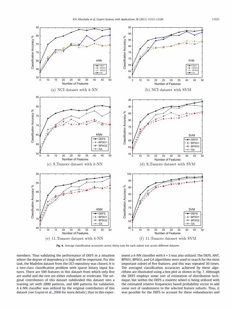
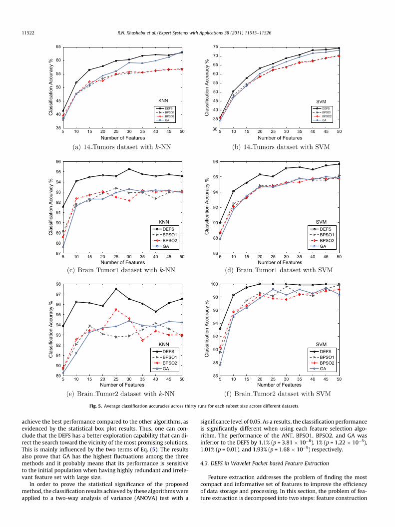
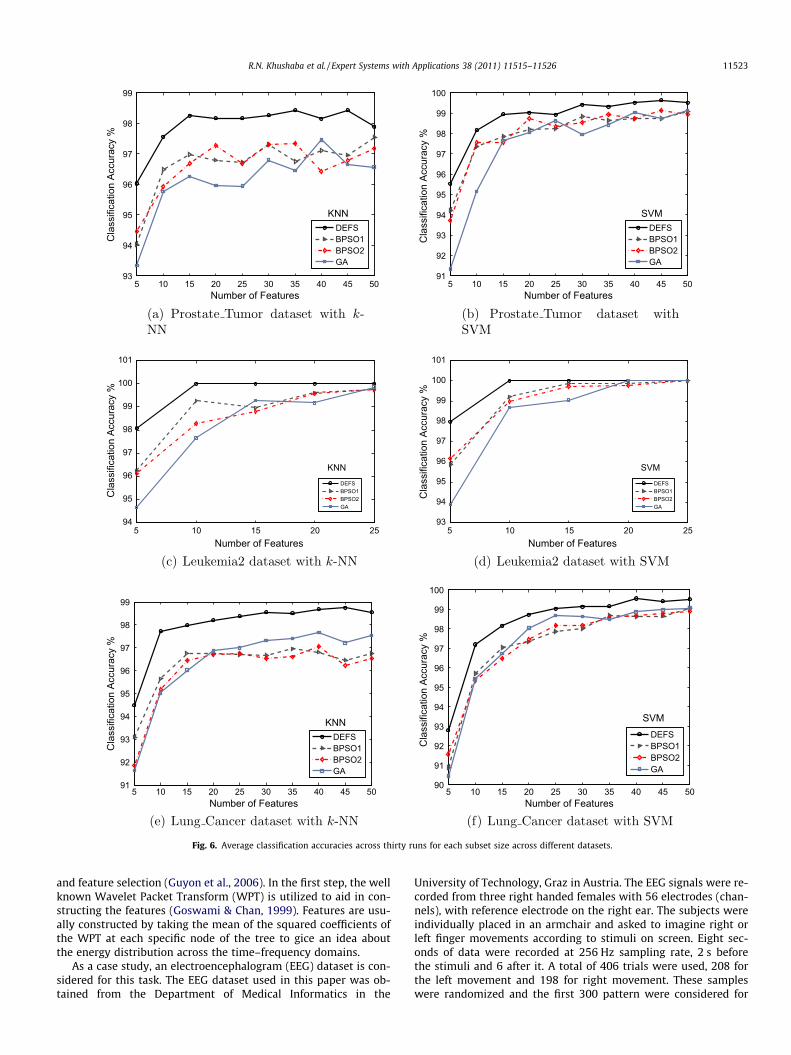
The constrained version of GA, BPSO1, and BPSO2 along withANT are used to select the most promising feature subsets for eachof the datasets shown in Table 1. The desired number of featurewas varied between 3 and 25 for the first four datasets and be-tween 5 and 50 for the remaining datasets. This was mainly donebecause it has been noticed that no improvement can be achievedwhen selecting larger number of features. For each subset size theexperiment was repeated 30 times, and the average classificationresults are shown in Figs. 3–6.

In order to analyze the results one can start by looking at theperformance of each of the BSPO1, BPSO2, and GA. It is very clearthat for almost all datasets the performance of BPSO1 and BPSO2methods is quite similar. The performance of GA on the other handis close to that of BPSO1 and BPSO2 in some datasets and a bit bet-ter in others. Since the probabilities of crossover and mutation inGA play an important role in the performance, several values weretested. These were made to change linearly and the values thatachieved the best performance were used in the experiments.The performance of DEFS proved to be better than that of BPSO1,BPSO2, and GA methods on all considered datasets. On the otherhand, the performance of DEFS is shown to be competing with thatof the ANT method across the different datasets, with DEFS show-ing slightly better results. One main difference between the ANTand DEFS in spite of the very similar performance is that the DEFShighly reduced the computational cost that is required by the ANTmethod. There are many factors that highly increase the computa-tional cost of the ANT method, these can be stated as: Firstly, theadditional computational cost for estimating the mutual informa-tion and the corresponding memory requirements to store thesematrices. As a simple example, on a Pentium 4 PC with 1 GByteof memory, it was impossible to run the Matlab code of the ANTon the NCI dataset as it ran out of memory (thus the ANT was omit-ted when dealing with huge datasets). Secondly, due to thesequential nature of the ANT-based feature selection method andthe ant colony optimization methods in general, the computationaltime was higher than that of DEFS, BPSO1, BPSO2, and GA, whereeach one of those algorithms has an embedded parallel compo-nent. As an example, consider a problem with the total numberof features being 4000 and the required subset size to be 50. Ifthe ANT method already selected five features then in order to se-lect the sixth feature it should estimate the pheromone intensitiesbetween the already selected five features and the remaining 3995.The same process is applied to select the seventh feature and so onto complete the subset of 50.

Thus all the results prove the effectiveness of the proposed DEFSin searching datasets of varying dimensionality for the best sub-sets. Although all of the methods started from the same initial pop-ulation, the continuous exploration ability of the DEFS that is aided

3 5 7 9 11 13 15 17 19 21 23 2570

75

80

85

90

95

100

Number of Feaures

Cla

ssifi

catio

n Ac

cura

cy %

DEFSANTBPSO1BPSO2GA

KNN

3 5 7 9 11 13 15 17 19 21 23 2570

75

80

85

90

95

100

Number of Feaures

Cla

ssifi

catio

n Ac

cura

cy %

DEFSANTBPSO1BPSO2GA

SVM

3 5 7 9 11 13 15 17 19 21 23 2590

91

92

93

94

95

96

97

98

99

Number of Feaures

Cla

ssifi

catio

n Ac

cura

cy %

DEFSANTBPSO1BPSO2GA

KNN

3 5 7 9 11 13 15 17 19 21 23 2590

91

92

93

94

95

96

97

98

99

100

Number of Feaures

Cla

ssifi

catio

n Ac

cura

cy %

DEFSANTBPSO1BPSO2GA

KNN

3 5 7 9 11 13 15 17 19 21 23 2575

80

85

90

95

100

Number of Feaures

Cla

ssifi

catio

n Ac

cura

cy %

DEFSANTBPSO1BPSO2GA

KNN

3 5 7 9 11 13 15 17 19 21 23 2575

80

85

90

95

100

Number of Feaures

Cla

ssifi

catio

n Ac

cura

cy %

DEFSANTBPSO1BPSO2GA

SVM

Fig. 3. Average classification accuracies across thirty runs for each subset size across different datasets.

11520 R.N. Khushaba et al. / Expert Systems with Applications 38 (2011) 11515–11526

by the statistical measure, proved to be very useful in searching thefeature space, hence outperforming all of the BPSO1, BPSO2, andGA. At the same time, the DEFS achieved close results to ANT withfar less computational cost.

4.2. Experiments on datasets with highly redundant features

Due to the fact that Estimation of Distribution Algorithms (EDA)that employ probability vectors usually allow only a very limited

representation of dependencies between features, as stated by Pel-ikan (2005), then it is tempting to validate the performance of DEFSon datasets with a large degree of dependency between features.Although the proposed DEFS is not exactly an EDA algorithm sinceit maintains a population of candidate solutions (unlike the EDAsthat replace the population with a probability distribution), butthe DEFS can be thought of as a mix of EDAs and real-valuedGAs. Within this mixture, the estimated probability vector is usedto replace the invalid (or duplicated) parts of the population

55

60

65

70

75

80

85

Cla

ssifi

catio

n Ac

cura

cy %

DEFSBPSO1BPSO2GA

KNN

55

60

65

70

75

80

85

90

95

Cla

ssifi

catio

n Ac

cura

cy %

DEFSBPSO1BPSO2GA

SVM

5 10 15 20 25 30 35 40 45 5055

60

65

70

75

80

85

Number of Features

Cla

ssifi

catio

n Ac

cura

cy %

DEFSBPSO1BPSO2GA

KNN

5 10 15 20 25 30 35 40 45 5055

60

65

70

75

80

85

90

95

Number of Features

5 10 15 20 25 30 35 40 45 50Number of Features

5 10 15 20 25 30 35 40 45 50Number of Features

Cla

ssifi

catio

n Ac

cura

cy %

DEFSBPSO1BPSO2GA

SVM

5 10 15 20 25 30 35 40 45 5065

70

75

80

85

90

95

Number of Features

Cla

ssifi

catio

n Ac

cura

cy %

DEFSBPSO1BPSO2GA

KNN

5 10 15 20 25 30 35 40 45 5060

65

70

75

80

85

90

95

100

Number of Features

Cla

ssifi

catio

n Ac

cura

cy %

DEFSBPSO1BPSO2GA

SVM

Fig. 4. Average classification accuracies across thirty runs for each subset size across different datasets.

R.N. Khushaba et al. / Expert Systems with Applications 38 (2011) 11515–11526 11521

members. Thus validating the performance of DEFS in a situationwhere the degree of dependency is high will be important. For thistask, the Madelon dataset from the UCI repository was chosen. It isa two-class classification problem with sparse binary input fea-tures. There are 500 features in this dataset from which only fiveare useful and the rest are either redundant or irrelevant. The ori-ginal contributors of this dataset subdivided this dataset into atraining set with 2000 patterns, and 600 patterns for validation.A k-NN classifier was utilized by the original contributors of thisdataset (see Guyon et al., 2006 for more details), thus in this exper-

iment a k-NN classifier with k = 3 was also utilized. The DEFS, ANT,BPSO1, BPSO2, and GA algorithms were used to search for the mostimportant subset of five features, and this was repeated 30 times.The averaged classification accuracies achieved by these algo-rithms are illustrated using a box plot as shown in Fig. 7. Althoughthe DEFS employs some sort of estimation of distribution tech-nique, but within the DEFS a roulette wheel is being utilized withthe estimated relative frequencies based probability vector to addsome sort of randomness to the selected feature subsets. Thus, itwas possible for the DEFS to account for these redundancies and

5 10 15 20 25 30 35 40 45 5035

40

45

50

55

60

65

Number of Features

Cla

ssifi

catio

n Ac

cura

cy %

DEFSBPSO1BPSO2GA

KNN

5 10 15 20 25 30 35 40 45 5030

35

40

45

50

55

60

65

70

75

Number of Features

Cla

ssifi

catio

n Ac

cura

cy %

DEFSBPSO1BPSO2GA

SVM

5 10 15 20 25 30 35 40 45 5087

88

89

90

91

92

93

94

95

96

Number of Features

Cla

ssifi

catio

n Ac

cura

cy %

DEFSBPSO1BPSO2GA

KNN

5 10 15 20 25 30 35 40 45 5086

88

90

92

94

96

98

Number of Features

Cla

ssifi

catio

n Ac

cura

cy %

DEFSBPSO1BPSO2GA

SVM

5 10 15 20 25 30 35 40 45 5089

90

91

92

93

94

95

96

97

98

Number of Features

Cla

ssifi

catio

n Ac

cura

cy %

DEFSBPSO1BPSO2GA

KNN

5 10 15 20 25 30 35 40 45 5086

88

90

92

94

96

98

100

Number of Features

Cla

ssifi

catio

n Ac

cura

cy %

DEFSBPSO1BPSO2GA

SVM

Fig. 5. Average classification accuracies across thirty runs for each subset size across different datasets.

11522 R.N. Khushaba et al. / Expert Systems with Applications 38 (2011) 11515–11526

achieve the best performance compared to the other algorithms, asevidenced by the statistical box plot results. Thus, one can con-clude that the DEFS has a better exploration capability that can di-rect the search toward the vicinity of the most promising solutions.This is mainly influenced by the two terms of Eq. (5). The resultsalso prove that GA has the highest fluctuations among the threemethods and it probably means that its performance is sensitiveto the initial population when having highly redundant and irrele-vant feature set with large size.

In order to prove the statistical significance of the proposedmethod, the classification results achieved by these algorithms wereapplied to a two-way analysis of variance (ANOVA) test with a

significance level of 0.05. As a results, the classification performanceis significantly different when using each feature selection algo-rithm. The performance of the ANT, BPSO1, BPSO2, and GA wasinferior to the DEFS by 1.1% (p = 3.81 � 10�8), 1% (p = 1.22 � 10�5),1.01% (p = 0.01), and 1.93% (p = 1.68 � 10�5) respectively.

4.3. DEFS in Wavelet Packet based Feature Extraction

Feature extraction addresses the problem of finding the mostcompact and informative set of features to improve the efficiencyof data storage and processing. In this section, the problem of fea-ture extraction is decomposed into two steps: feature construction

5 10 15 20 25 30 35 40 45 5093

94

95

96

97

98

99

Number of Features

Cla

ssifi

catio

n Ac

cura

cy %

DEFSBPSO1BPSO2GA

KNN

5 10 15 20 25 30 35 40 45 5091

92

93

94

95

96

97

98

99

100

Number of Features

Cla

ssifi

catio

n Ac

cura

cy %

DEFSBPSO1BPSO2GA

SVM

5 10 15 20 2594

95

96

97

98

99

100

101

Number of Features

Cla

ssifi

catio

n Ac

cura

cy %

DEFSBPSO1BPSO2GA

KNN

5 10 15 20 2593

94

95

96

97

98

99

100

101

Number of Features

Cla

ssifi

catio

n Ac

cura

cy %

DEFSBPSO1BPSO2GA

SVM

5 10 15 20 25 30 35 40 45 5091

92

93

94

95

96

97

98

99

Number of Features

Cla

ssifi

catio

n Ac

cura

cy %

DEFSBPSO1BPSO2GA

KNN

5 10 15 20 25 30 35 40 45 5090

91

92

93

94

95

96

97

98

99

100

Number of Features

Cla

ssifi

catio

n Ac

cura

cy %

DEFSBPSO1BPSO2GA

SVM

Fig. 6. Average classification accuracies across thirty runs for each subset size across different datasets.

R.N. Khushaba et al. / Expert Systems with Applications 38 (2011) 11515–11526 11523

and feature selection (Guyon et al., 2006). In the first step, the wellknown Wavelet Packet Transform (WPT) is utilized to aid in con-structing the features (Goswami & Chan, 1999). Features are usu-ally constructed by taking the mean of the squared coefficients ofthe WPT at each specific node of the tree to gice an idea aboutthe energy distribution across the time–frequency domains.

As a case study, an electroencephalogram (EEG) dataset is con-sidered for this task. The EEG dataset used in this paper was ob-tained from the Department of Medical Informatics in the

University of Technology, Graz in Austria. The EEG signals were re-corded from three right handed females with 56 electrodes (chan-nels), with reference electrode on the right ear. The subjects wereindividually placed in an armchair and asked to imagine right orleft finger movements according to stimuli on screen. Eight sec-onds of data were recorded at 256 Hz sampling rate, 2 s beforethe stimuli and 6 after it. A total of 406 trials were used, 208 forthe left movement and 198 for right movement. These sampleswere randomized and the first 300 pattern were considered for

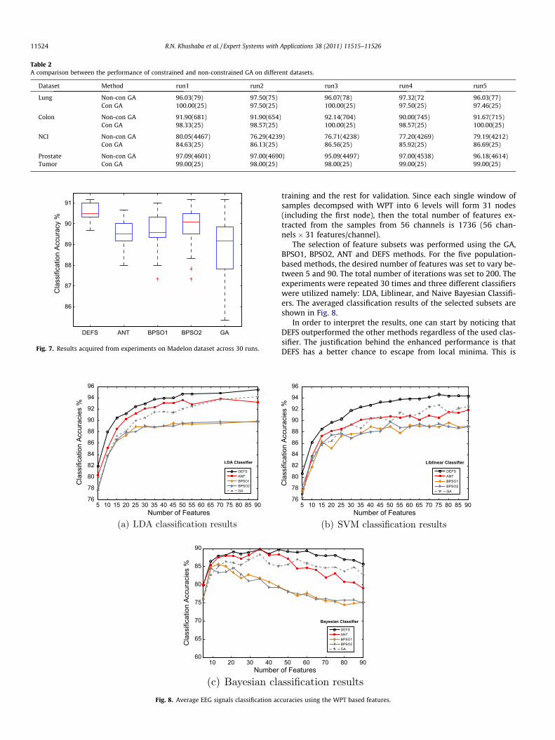
Table 2A comparison between the performance of constrained and non-constrained GA on different datasets.

Dataset Method run1 run2 run3 run4 run5

Lung Non-con GA 96.03(79) 97.50(75) 96.07(78) 97.32(72 96.03(77)Con GA 100.00(25) 97.50(25) 100.00(25) 97.50(25) 97.46(25)

Colon Non-con GA 91.90(681) 91.90(654) 92.14(704) 90.00(745) 91.67(715)Con GA 98.33(25) 98.57(25) 100.00(25) 98.57(25) 100.00(25)

NCI Non-con GA 80.05(4467) 76.29(4239) 76.71(4238) 77.20(4269) 79.19(4212)Con GA 84.63(25) 86.13(25) 86.56(25) 85.92(25) 86.69(25)

Prostate Non-con GA 97.09(4601) 97.00(4690) 95.09(4497) 97.00(4538) 96.18(4614)Tumor Con GA 99.00(25) 98.00(25) 98.00(25) 99.00(25) 99.00(25)

DEFS ANT BPSO1 BPSO2 GA

86

87

88

89

90

91

Cla

ssifi

catio

n Ac

cura

cy %

Fig. 7. Results acquired from experiments on Madelon dataset across 30 runs.

5 10 15 20 25 30 35 40 45 50 55 60 65 70 75 80 85 9076

78

80

82

84

86

88

90

92

94

96

Number of Features

Cla

ssifi

catio

n Ac

cura

cies

%

DEFSANTBPSO1BPSO2GA

LDA Classifier

10 20 30 4060

65

70

75

80

85

90

Number

Cla

ssifi

catio

n Ac

cura

cies

%

Fig. 8. Average EEG signals classification ac

11524 R.N. Khushaba et al. / Expert Systems with Applications 38 (2011) 11515–11526

training and the rest for validation. Since each single window ofsamples decompsed with WPT into 6 levels will form 31 nodes(including the first node), then the total number of features ex-tracted from the samples from 56 channels is 1736 (56 chan-nels � 31 features/channel).

The selection of feature subsets was performed using the GA,BPSO1, BPSO2, ANT and DEFS methods. For the five population-based methods, the desired number of features was set to vary be-tween 5 and 90. The total number of iterations was set to 200. Theexperiments were repeated 30 times and three different classifierswere utilized namely: LDA, Liblinear, and Naive Bayesian Classifi-ers. The averaged classification results of the selected subsets areshown in Fig. 8.

In order to interpret the results, one can start by noticing thatDEFS outperformed the other methods regardless of the used clas-sifier. The justification behind the enhanced performance is thatDEFS has a better chance to escape from local minima. This is

5 10 15 20 25 30 35 40 45 50 55 60 65 70 75 80 85 9076

78

80

82

84

86

88

90

92

94

96

Number of Features

Cla

ssifi

catio

n Ac

cura

cies

%

DEFSANTBPSO1BPSO2GA

Liblinear Classifier

50 60 70 80 90of Features

DEFSANTBPSO1BPSO2GA

Bayesian Classifier

curacies using the WPT based features.

R.N. Khushaba et al. / Expert Systems with Applications 38 (2011) 11515–11526 11525

mainly caused by the fact that the float-optimization engine of theDEFS will always cause replication of certain features, thus there isalways a need for finding suitable replacement for the replicatedportions, which is done using the probability vector and the rou-lette wheel. Accordingly, there is a sort of continuous explorationand exploitation capability associated with the DEFS search proce-dure. Also, because the probability is being updated with each iter-ation, this process will give the DEFS a better capability of findingthe features that constitute the best subsets.

On the other hand, the ANT showed good performance on smallsubsets while showing a degraded performance with large subsets.This is due to the fact that ANT builds an approximation of the sub-sets importance using mutual information, which is done using ahistogram approach that can become less reliable as the numberof features increases. Another factor could be the sequential natureof the ANT method. The performance of GA was found to be notvery competitive when selecting small number of features. Thiscould be related to the cross-over and mutation operators, as theymay fail to lead the search for the best small subset toward the glo-bal minima when dealing with huge datasets. However, as thenumber of selected features increases, the performance of GA gotbetter, and in fact it managed to achieve better results than BPSO1,BPSO2, and even ANT. The reason for the unstable performance ofboth of BPSO1 and BPSO2 based feature selection might be justifiedby the fact that both methods can get stuck into local minimawhen dealing with large datasets. Thus one can deduce that theperformance of DEFS was more acceptable than all other methodsin this experiment.

5. Conclusion

A new feature selection method was developed in this paperbased on modifying the DE float-number optimizer. The justifica-tion behind the need for the proposed DEFS was explained. A rangeof datasets with various dimensionality and number of target clas-ses were considered to test the performance of the DEFS. Themethod was compared with many other population based featureselection methods and the results proves the superiority of theproposed method in most cases. Finally, the DEFS was utilized asa part of WPT based feature extraction process presenting powerfulresults in searching for subsets of features/channels that best inter-act together.

Appendix A. Matlab code for the constrained GA crossover

The following is the Matlab code for the constrained GAcrossover.

01.

function kid = Fix_GA (ptr1,ptr2,NOF,DNF)

02.

kid = zeros (1,NOF)%initialize the kid

03.

kkk = 0;

04.

While kkk == 0

05.

%crossover parents to get the kid

06.

for j = 1 :NOF

07.

if (rand > 0.5) 08. kid (j) = prt1(j);

09.

else

10.

kid (j) = prt2(j);

11.

end

12.

%get all features from parents

13.

smu = unique ([find (prt1) find (prt2)]);

14.

%sm1 = the common features between parents

15.

sm1 = intersect (find (prt1), find (prt2));

16.

%sm0 = Kid � intersect of parents

17.

sm0 = setdiff (find (kd),sm1);

18.

%sm1 = Union of the two parents � Kid

19.

sm1 = setdiff (smu,find (kd));

20.

rsm0 = randperm (length (sm0));

21.

rsm1 = randperm (length (sm1));

22.

% Turn off additional bits

23.

for z = 1:sum (kid) � DNF,

24.

kid (sm0(rsm0(z))) = 0;

25.

end

26.

% Turn on additional bits

27.

for z = 1:DNF-sum (kid),

28.

kid (sm1(rsm1(z))) = 1;

29.

end

30.

% check for termination

31.

if sum (kid) == DNF

32.

kkk = 1;

33.

end

34.

end

Appendix B. Matlab code for the constrained PSO

The following is the Matlab code for the constrained PSO.

01.

function kid = Fix_PSO (SVelocity,NOF,DNF)

02.

% SVelocity: particlesvsquashed velocity

03.

% SVelocity = 1/(1 + exp (�Velocity)) 04. % Now sort the resultant velocity indices

05.

[vSVel ind] = sort (SVelocity,‘descend’);

06.

while kkk == 1

07.

% initialize kid as empty vector

08.

kid = [];

09.

% initialize kid length to zero

10.

len_kid = 0; 11. for j = 1:NOF

12.

if vSVel (j) > rand & len_kid < DNF 13. kid = [kid ind (j)];

14.

len_kid = length (kid);

15.

end

16.

end

17.

if len_kid == DNF 18. kkk = 0;

19.

end

20.

end

References

Aghdam, M. H., Aghaee, N. G., & Basiri, M. E. (2008). Text feature selection using antcolony optimization. Expert Systems with Applications, 36(2, Part2), 6843–6853.

Al-Ani, A. (2005). Feature subset selection using ant colony optimization.International Journal of Computational Intelligence, 2(1), 53–58.

Bergh, F. V. D. (2001). An analysis of particle swarm optimizers. PhD thesis, Universityof Pretoria, Pretoria, South Africa.

Brill, F. Z., Brown, D. E., & Martin, W. N. (1992). Fast genetic selection of featuresfor neural network classifiers. IEEE Transactions on Neural Networks, 3(2),324–328.

Chuang, L. Y., Chang, H. W., Tu, C. J., & Yang, C. H. (2008). Improved binary pso forfeature selection using gene expression data. Computational Biology andChemistry, 32(1), 29–38.

Dorigo, M., & Stutzle, T. (2004). Ant colony optimization. London: MIT Press.Firpi, H. A., & Goodman, E. (2004). Swarmed feature selection. In Proceedings of the

33rd applied imagery pattern recognition workshop (pp. 112–118).Glover, F., & Laguna, M. (1997). Tabu search. Kluwer Academic Publishers.Goswami, J. C., & Chan, A. K. (1999). Fundamentals of wavelets: Theory algorithms, and

applications. New York: Wiley.Guyon, I., Gunn, S., Nikravesh, M., & Zadeh, L. A. (2006). Feature extraction:

Foundations and applications. Netherlands: Springer-Verlag, Berlin, Heidelberg.Haupt, R. L., & Haupt, S. E. (2004). Practical genetic algorithms (2nd ed.). John Wiley

and Sons.Jensen, R., & Shen, Q. (2008). Computational intelligence and feature selection.

Hoboken, New Jersey: John Wiley and Sons, Inc.

11526 R.N. Khushaba et al. / Expert Systems with Applications 38 (2011) 11515–11526

Kanan, H. R., & Faez, K. (2008a). Ga-based optimal selection of pzmi features for facerecognition. Applied Mathematics and Computation, 205(2), 706–715.

Kanan, H. R., & Faez, K. (2008b). An improved feature selection method based on antcolony optimization (ACO) evaluated on face recognition system. AppliedMathematics and Computation, 205(2), 716–725.

Kennedy, J., Eberhart, R. C., & Shi, Y. (2001). Swarm intelligence. London: MorganKaufman Publishers.

Laarhoven, P. J. M., & Aarts, E. H. L. (1988). Simulated annealing: Theory andapplications. Kluwer Academic Publishers.

Liu, H., Dougherty, E. R., Dy, J. G., Torkkola, K. A., Tuv, E., Peng, H. A., et al. (2005).Evolving feature selection. IEEE Intelligent Systems, 20(6), 64–76.

Liu, H., & Motoda, H. (2008). In H. Liu, & H. Motoda (Eds.), Less is more inComputational methods of feature selection (pp. 3–17). New York, USA: Taylorand Francis Group, LLC.

Lu, J., Zhao, T., & Zhang, Y. (2008). Feature selection based-on genetic algorithm forimage annotation. Knowledge-Based Systems, 21(8), 887–891.

Oh, I. S., Lee, J. S., & Moon, B. R. (2004). Hybrid genetic algorithms for featureselection. IEEE Transactions on Pattern Analysis and Machine Intelligence, 26(11),1424–1437.

Palit, A. K., & Popovic, D. (2005). Computational intelligence in time series forecasting:Theory and engineering applications. Springer.

Pelikan, M. (2005). Hierarchical Bayesian optimization algorithm: Toward a newgeneration of evolutionary algorithms. Springer.

Price, K. V., Storn, R. M., & Lampinen, J. A. (2005). Differential evolution: A practicalapproach to global optimization. Springer.

Raymer, M. L., Punch, W. F., Goodman, E. D., Kuhn, L. A., & Jain, A. K. (2000).Dimensionality reduction using genetic algorithms. IEEE Transactions onEvolutionary Computation, 4(2), 164–171.