Feasibility of multi-temporal interferometric SAR data for stand-level estimation of boreal forest...

Feasibility of multi-temporal interferometric SAR data for stand-level

estimation of boreal forest stem volume

Jouni Pulliainen*, Marcus Engdahl, Martti Hallikainen

Laboratory of Space Technology, Helsinki University of Technology, Otakaari 5A, P.O. Box 3000, Espoo FIN-02015 HUT, Finland

Received 10 June 2002; received in revised form 23 December 2002; accepted 31 December 2002

Abstract

The feasibility of interferometric SAR (INSAR) coherence observations for stem volume (biomass) retrieval is investigated by applying

coherence data determined from 14 ERS-1 and ERS-2 C-band SAR image pairs. The image set covers a single forested test area in Finland,

and both summer (snow-free) and winter conditions are represented. The data set enabled (a) the study of stem volume retrieval performance

under varying conditions, (b) the analysis of the seasonal behavior of interferometric coherence, and (c) the determination of the accuracy

characteristics of empirical (nonlinear) coherence modeling. Additionally, a new technique to estimate forest stem volume from INSAR data

was developed based on constrained iterative inversion of the applied empirical model. The results indicate that the usability of winter images

with snow-covered terrain is superior to that of images obtained under summer conditions. The applied empirical model appears to be

adequate for describing the stand-wise coherence of boreal forest. Hence, a practical stem volume estimation method can be established based

on it. The highest correlation coefficient between the estimated stem volume and the ground truth stem volume showed values as high as

r = 0.9 and a relative RMSE level of 48% was obtained, respectively.

D 2003 Elsevier Science Inc. All rights reserved.

Keywords: Remote sensing of forests; Radar interferometry

1. Introduction

Forest stem volume is one of the key characteristics in

forest inventories. It is as well an essential characteristic for

forest and climatological research, as it is a figure directly

related to the level of total forest biomass. Satellite sensors

have shown to be useful for mapping forest stem volume for

large areas, but their accuracy for small areas, such as

individual forest stands with a typical size of a couple of

hectares, is poor. Possibilities to improve this handicap

include the use of high spatial resolution satellite data

(resolution in the order of few meters) and the use of

advanced measurement techniques, such as interferometric

SAR (INSAR), with a poorer spatial resolution (but con-

sequently with a larger imaging area).

Previous investigations have shown that the interfero-

metric coherence measured by a spaceborne INSAR sys-

tem is highly affected by the forest biomass (stem volume).

Especially, in the case of sparse boreal forests, INSAR

appears to be a promising data source, see, e.g. Askne,

Dammert, Ulander, and Smith (1997) and Koskinen, Pull-

iainen, Hyyppa, Engdahl, and Hallikainen (2001). How-

ever, problems arise due to the strong influence of weather

conditions. The sensitivity of interferometric radar response

to biomass can drop close to zero at its worst. Never-

theless, the results obtained in stem volume retrieval have

shown relatively good performances, comparable to those

obtained with optical satellite sensors, as multi-temporal

INSAR data are employed (Askne, Santoro, Smith, &

Fransson, 2002; Fransson, Smith, Askne, & Olsson,

2001; Koskinen et al., 2001; Santoro, Askne, Dammert,

Fransson, & Smith, 1999; Santoro, Askne, Smith, &

Fransson, 2002).

The modeling of interferometric coherence is a compli-

cated task as detailed models should describe both the

amplitude and phase of signals backscattered from the

forested terrain including the decorrelation of received

signals due to random phase shifts. These shifts are caused,

e.g. by volume scattering and by the movement of individ-

ual scatterers (the latter being the reason for temporal

decorrelation in repeat-pass interferometry), see, e.g. Treu-

haft and Siqueira (2000) and Zebker and Villasenor (1992).

0034-4257/03/$ - see front matter D 2003 Elsevier Science Inc. All rights reserved.

doi:10.1016/S0034-4257(03)00016-6

* Corresponding author. Tel.: +358-9-451-2373; fax: +358-9-451 2898.

E-mail address: [email protected] (J. Pulliainen).

www.elsevier.com/locate/rse

Remote Sensing of Environment 85 (2003) 397–409

However, recent investigations have indicated that rela-

tively simple empirical or semi-empirical models are fea-

sible to describe the average behavior of interferometric

coherence as a function of forest stem volume or tree height

(Askne et al., 1997; Koskinen et al., 2001). This makes it

possible to develop coherence model-based inversion tech-

niques to estimate the level of forest stem volume or

biomass.

The model by Askne et al. (1997) is a physically

detailed model describing the coherence as a function of

stem volume, (perpendicular) baseline length, and tree

height which can be expressed as a function of stem

volume. The model of Koskinen et al. (2001) is a simpler

formulation that only includes the effect of stem volume.

Both formulations are based on the semi-empirical model-

ing of forest canopy backscatter as a function of stem

volume, see, e.g. Pulliainen, Heiska, Hyyppa, and Hallikai-

nen (1994).

The methods used for the retrieval of stem volume

include empirical and semi-empirical (model-based)

approaches. Wagner et al. (2000) employed a nonlinear

empirical formula for relating the coherence to stem

volume in classifying Siberian forests into two stem

volume classes from a mosaic of single ERS-1/2 Tandem

INSAR images. Fransson et al. (2001), Hyyppa et al.

(2000), and Koskinen et al. (2001) applied simple and

multiple linear regression formulas for the determination of

stem volume from ERS-1/2 coherence (and intensity)

images. Askne et al. (2002), Santoro et al. (1999), and

Santoro et al. (2002) demonstrated semi-empirical stem

volume retrieval approaches based on the model by Askne

et al. (1997).

In this study, we introduce a novel stem volume retrieval

method that is based on the empirical backscattering–

coherence model presented by Koskinen et al. (2001). The

differences between the introduced technique and the non-

linear approach used by Santoro et al. (2002) include the

following aspects.

(a) The method used by Santoro et al. (2002) applies the

coherence model by Askne et al. (1997), whereas this

investigation uses the model introduced by Koskinen et

al. (2001). The underlying backscattering model has

some differences as well. The HUT boreal forest

backscattering model employed here has two empirical

parameters, whereas the model used by Santoro et al.

(2002) is a three-parameter formulation.

(b) The introduced method is based on the constrained

statistical inversion approach (Lehtinen, 1988) in which

the maximum likelihood of the stem volume value is

searched when multi-temporal observations are jointly

given. The approach by Santoro et al. (2002) separately

estimates the stem volume for each coherence image,

and linearly combines the estimates with specific

weighting factors (these factors are affected by the

residuals of model fittings).

The performance of the employed stem volume

retrieval method is analyzed by using a coherence data

set determined from 14 ERS-1 and ERS-2 C-band SAR

image pairs. For comparison, the stem volume estimates

are also determined with standard multiple linear regres-

sion approach. The applied image set covers a single test

area in Southern Finland, and both summer (snow-free)

and winter conditions are represented (1 year time span

from July 1995 to July 1996 is covered). The main

reference information includes ground-based forest inven-

tory data determined at stand level. The data set also

enables the analysis of the seasonal behavior of inter-

ferometric coherence and the investigation of the accu-

racy characteristics of empirical nonlinear coherence

modeling.

2. Methods and SAR data processing

This section describes the empirical backscattering–

coherence model and the inversion approach developed

based on the model. Additionally, the model by Askne et

al. (1997) is presented for comparison. The processing of

interferometric coherence data is also described in detail as

that issue is an essential factor regarding the quality of

interferometric coherence information. In practice, the accu-

racy of stem volume retrieval is highly affected by the

quality of data processing.

2.1. Empirical coherence modeling and model inversion

2.1.1. Modeling approach

The empirical coherence modeling is based on the HUT

boreal forest backscattering model that describes the C- and

X-band backscattering coefficient of forested areas as a

function of forest stem volume and takes into account the

effects of vegetation water content, top-soil moisture, and

the effective surface roughness (Koskinen et al., 2001;

Pulliainen et al., 1994; Pulliainen, Kurvonen, & Hallikai-

nen, 1999; Pulliainen, Mikkela, Hallikainen, & Ikonen,

1996). The model has been validated for conifer-dominated

boreal forests using C- and X-band airborne ranging scat-

terometer data and C-band spaceborne SAR observations,

especially ERS-1/2 SAR data. Observations used for model

validation were collected during the years 1992–1997 for

four geographical regions in Finland representing ecologi-

cally southern and northern boreal forests. The data repre-

sent both wintertime and snow-free summer conditions. The

detailed in situ reference data used for model validation

include field inventory data from a total of 1000 forest

stands, and from hundreds of smaller sample plots and

transects.

In case of ERS SAR observations (i.e. for C-band, VV-

polarized observations at 23j angle of incidence), the

average backscattering coefficient rj of forested terrain

can be approximately modeled ignoring trunk-ground and

J. Pulliainen et al. / Remote Sensing of Environment 85 (2003) 397–409398

other multiple scattering mechanisms (Koskinen et al.,

2001; Pulliainen et al., 1999) by

rjðV ; h;mv;can; rgroundj Þ ¼rcanj ðV ; h;mv;canÞþ t2ðV ; h;mv;canÞrgroundj

urcanjþ rfloorj ð1Þ

where rgroundj is the ground layer backscatter. The canopy

backscattering contribution rcanj is equal to

rcanj ðV ; h;mv;canÞ¼rV ðh;mv;canÞcosðhÞ

2jeðh;mv;canÞð1� t2ðV ; h;mv;canÞÞ

ð2Þ

and the two-way forest canopy transmissivity t2 is equal to

t2ðV ; h;mv;canÞ ¼ expð�2jeðh;mv;canÞV=coshÞ ð3Þ

In Eqs. (1)–(3), V is the total stem volume of forest

(forest stand), h is the angle of incidence, and mv,can is the

effective vegetation (forest canopy) volumetric water con-

tent. The forest canopy extinction and volume backscatter-

ing coefficients (je and rV, respectively) are the parameters

retrieved from scatterometer observations originally

(jefmv and rVfmv2).In this study, we can reduce the

influence of parameters je, rV, and rjground in Eqs. (1)–(3)

into two empirical coefficients that can be estimated based

on inversion algorithm reference (training) data that must be

available from the study region. Hence, the boreal forest

backscattering model (1) can be rewritten for the case of

ERS 1/2 SAR observations (absolute rj level determined

according to SLC image calibration coefficient data) as

rjðV ; hÞ ¼ 0:131acosh 1� exp �5:12� 10�3 aV

cosh

� ��

þ bexp �5:12� 10�3 aV

cosh

� �urcanj þ rfloorj

ð4Þ

where parameter a is related to the volumetric vegetation

water content (under dry summer conditions a is close to 1)

and parameter bu rjground. Based on Koskinen et al. (2001)

the level of interferometric coherence as a function of forest

stem volume V is linearly dependent on the ratio rcano (V)/ro

(V) (note that h is omitted here and onwards for simplicity).

Hence, the interferometric coherence AcA can be modeled

by

AcðV ÞA ¼ c0 þ c1rcanj ða;V Þrjða; b;V Þ

� �ð5Þ

where c0 and c1 are empirical coefficients that have to be

determined from reference (training) data. As stated in

Koskinen et al. (2001) c0 corresponds to the level of

coherence for open areas, i.e. clear-cut or sapling areas

(V= 0 m3/ha), and c1 corresponds to the difference between

coherence levels of very dense forests and open areas.The

performance of the model (5) can be compared with that of

the model by Askne et al. (1997). The model (5) can be

rewritten as

AcðV ÞA ¼ c0rfloorj ða; b;V Þ

rjða; b;V Þ

� �þ ðc0 þ c1Þ

rcanj ða;V Þrjða; b;V Þ

� �ð6Þ

Similarly, the coherence model used by Askne et al. (1997)

and Santoro et al. (2002) can be expressed as

AcðV ÞA ¼ cgrrfloorj ða; b;V Þ

rjða; b;V Þ

� �þ ccan

rcanj ða;V Þrjða; b;V Þ

� �� exp �j

4pBn

kRsinhðh� a�1Þ

� �� ð7Þ

where cgr is the coherence level of ground and ccan is that ofthe forest canopy, respectively. j is the imaginary unit, Bn is

the perpendicular length of the interferometric baseline, R is

the slant range, k is the radar wavelength, h is the height of

forest canopy and a is the two-way attenuation of the forest

canopy (Askne et al., 1997). Based on the forest stand data

on stem volume (V) and mean tree height (h) of the present

test site (the Tuusula test site), the same relation between V

and h can be used here as that in Santoro et al. (2002), i.e.

h=(2.44V)0.46.One should note that Eq. (7) reduces to Eq.

(6) if Bn = 0 m.

2.1.2. Inversion technique

The developed inversion technique is based on the

statistical inversion approach (Lehtinen, 1988). In prac-

tice, a three-step minimization procedure is established.

The algorithm requires that ground reference data on

forest stem volume are available for training regions.

The actual minimization problems can be solved with

standard (constrained) iteration algorithms. In the case of

ERS INSAR data, the first step of the algorithm is the

fitting of backscattering model (curve as a function of V)

given by Eq. (4) to observed mean rj values of all

training regions with a and b as parameters to be

optimized

mina;b

XNi¼1

wiðrmodeledj ða; b;ViÞ � robserved;ij Þ2 ð8Þ

where rmodeledo is the backscattering coefficient predicted

by Eq. (4). Vi is the known value of forest stem volume

for the training forest stand number i. robserved,io is the

mean backscattering coefficient observed for the training

region i (mean value of the two intensity images used for

J. Pulliainen et al. / Remote Sensing of Environment 85 (2003) 397–409 399

the calculation). The total number of training regions is

N. The optional weighing factor wi is related to the

proportional area of the region i

wi ¼ Ai

XNi¼1

Ai

,ð9Þ

The second phase is the fitting of coherence model (5)

into interferometric coherence data by optimizing c0 and

c1. Again, this is performed for the training data set by

applying a and b values estimated at the first phase of the

algorithm. Let the estimated values of a and b be a and

b, then the minimization problem is stated as

minc0;c1

XNi¼1

wiðAcðc0; c1ÞAmodeled;i � AcAobserved;iÞ2

as Acðc0; c1ÞAmodeled;i ¼ Acðc0; c1;Vi; a; bÞA ð10Þ

The outcome of the nonlinear optimization procedure (Eq.

(10)) is the estimates c0 and c1.

The third phase of the algorithm is the estimation of

forest stem volume for any forest region, which can be

carried out using multi-temporal INSAR data (optimizations

according to Eqs. (9) and (10) are carried out separately for

each individual image). If the stem volume estimation is

carried out using a total of m images, the minimization

problem to retrieve forest stem volume for the forest region j

is given by

minVj

Xmk¼1

WkðAcðVjÞAmodeled;k � AcAobserved;k;jÞ2

such that Vjz 0 m3/ha as

AcðVjÞAmodeled;k ¼ AcðVj; c0;k ; c1;k ; ak ; bkÞA ð11Þ

where Wk is weight factor determined by the residuals of

model fitting (Eq. (10))

Wk ¼1

2VarðRkÞð12Þ

where Rk is the residual vector obtained for the training

regions of image k

Rk ¼�AcAk

modeled;1 � AcAkobserved;1 AcAk

modeled;2

� AcAkobserved;2 . . .AcAk

modeled;N � AcAkobserved;N

�ð13Þ

It can be shown that Eq. (11) yields a maximum like-

lihood estimate on forest stem volume given the radar

observations, if the error of model (5) has a Gaussian

distribution. Moreover, if the distribution of stem volume

is Gaussian around its mean value, the maximum like-

lihood estimate of stem volume is obtained based on

Bayes theorem by

minVj

Xmk¼1

WkðAcðVjÞAmodeled;k �AcAobserved;k;jÞ2

þ 1

2Varð½V1; . . . ;VN �ÞVj �

1

N

XNi¼1

Vi

!2

ð14Þ

such that Vjz 0 m3/ha.

Even though the forest stem volume does not typically

obey Gaussian distribution, the use of regulating sum term

can be useful, as it often reduces the retrieval bias by

shifting the estimates toward the mean value of the training

data set.

An important aspect of the multi-temporal inversion

technique is its ability to compensate for the random

fluctuations of individual observations. Even though the

observed coherence value for an individual stand may be

lower than the minimum modeled coherence values for the

highest stem volumes, the estimates determined from multi-

ple observations do not (typically) show unrealistically high

values. The bias term included in Eq. (12) emphasizes this

effect.

2.2. INSAR data processing

2.2.1. SAR data

The SAR data used in this study consist of 14 ERS-1/2

Tandem image pairs (28 SLC images in total) acquired with

the C-band SARs on-board the European Space Agency’s

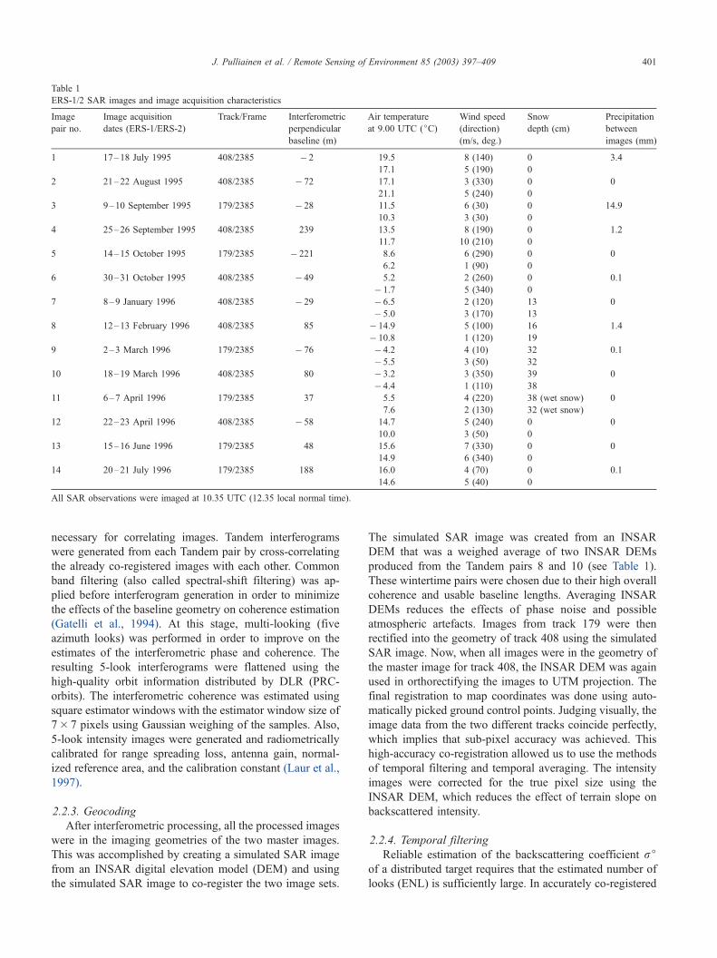
ERS-1 and ERS-2 satellites. Table 1 summarizes the key

imaging characteristics and the weather conditions during

the image acquisition (all the images were acquired from

descending orbits). The imagery was acquired during the

ERS-1/2 Tandem mission in 1995–1996, when the two

satellites were flown in the same orbital plane so that ERS-2

imaged the same area on the ground 24 h after ERS-1. Due

to the relatively short temporal baseline of 24 h and the short

interferometric baselines, the image pairs collected during

the Tandem mission are useful in interferometric studies of

natural targets, which decorrelate quite rapidly in C-band.

The image data used in this study span a whole year from

the summer of 1995 to the summer of 1996.

2.2.2. Interferometric processing

Interferometric processing and geocoding of the SAR

image data were done using a software package described in

Wegmuller, Werner, and Strozzi (1998). Since the data were

from two different imaging geometries depending on the

track/frame combination, the images were processed in two

separate sets. First, a master image was chosen for both

geometries, and all images were co-registered to their

respective master image with sub-pixel accuracy that is


necessary for correlating images. Tandem interferograms

were generated from each Tandem pair by cross-correlating

the already co-registered images with each other. Common

band filtering (also called spectral-shift filtering) was ap-

plied before interferogram generation in order to minimize

the effects of the baseline geometry on coherence estimation

(Gatelli et al., 1994). At this stage, multi-looking (five

azimuth looks) was performed in order to improve on the

estimates of the interferometric phase and coherence. The

resulting 5-look interferograms were flattened using the

high-quality orbit information distributed by DLR (PRC-

orbits). The interferometric coherence was estimated using

square estimator windows with the estimator window size of

7� 7 pixels using Gaussian weighing of the samples. Also,

5-look intensity images were generated and radiometrically

calibrated for range spreading loss, antenna gain, normal-

ized reference area, and the calibration constant (Laur et al.,

1997).

2.2.3. Geocoding

After interferometric processing, all the processed images

were in the imaging geometries of the two master images.

This was accomplished by creating a simulated SAR image

from an INSAR digital elevation model (DEM) and using

the simulated SAR image to co-register the two image sets.

The simulated SAR image was created from an INSAR

DEM that was a weighed average of two INSAR DEMs

produced from the Tandem pairs 8 and 10 (see Table 1).

These wintertime pairs were chosen due to their high overall

coherence and usable baseline lengths. Averaging INSAR

DEMs reduces the effects of phase noise and possible

atmospheric artefacts. Images from track 179 were then

rectified into the geometry of track 408 using the simulated

SAR image. Now, when all images were in the geometry of

the master image for track 408, the INSAR DEM was again

used in orthorectifying the images to UTM projection. The

final registration to map coordinates was done using auto-

matically picked ground control points. Judging visually, the

image data from the two different tracks coincide perfectly,

which implies that sub-pixel accuracy was achieved. This

high-accuracy co-registration allowed us to use the methods

of temporal filtering and temporal averaging. The intensity

images were corrected for the true pixel size using the

INSAR DEM, which reduces the effect of terrain slope on

backscattered intensity.

2.2.4. Temporal filtering

Reliable estimation of the backscattering coefficient rjof a distributed target requires that the estimated number of

looks (ENL) is sufficiently large. In accurately co-registered

Table 1

ERS-1/2 SAR images and image acquisition characteristics

Image

pair no.

Image acquisition

dates (ERS-1/ERS-2)

Track/Frame Interferometric

perpendicular

baseline (m)

Air temperature

at 9.00 UTC (jC)Wind speed

(direction)

(m/s, deg.)

Snow

depth (cm)

Precipitation

between

images (mm)

1 17–18 July 1995 408/2385 � 2 19.5 8 (140) 0 3.4

17.1 5 (190) 0

2 21–22 August 1995 408/2385 � 72 17.1 3 (330) 0 0

21.1 5 (240) 0

3 9–10 September 1995 179/2385 � 28 11.5 6 (30) 0 14.9

10.3 3 (30) 0

4 25–26 September 1995 408/2385 239 13.5 8 (190) 0 1.2

11.7 10 (210) 0

5 14–15 October 1995 179/2385 � 221 8.6 6 (290) 0 0

6.2 1 (90) 0

6 30–31 October 1995 408/2385 � 49 5.2 2 (260) 0 0.1

� 1.7 5 (340) 0

7 8–9 January 1996 408/2385 � 29 � 6.5 2 (120) 13 0

� 5.0 3 (170) 13

8 12–13 February 1996 408/2385 85 � 14.9 5 (100) 16 1.4

� 10.8 1 (120) 19

9 2–3 March 1996 179/2385 � 76 � 4.2 4 (10) 32 0.1

� 5.5 3 (50) 32

10 18–19 March 1996 408/2385 80 � 3.2 3 (350) 39 0

� 4.4 1 (110) 38

11 6–7 April 1996 179/2385 37 5.5 4 (220) 38 (wet snow) 0

7.6 2 (130) 32 (wet snow)

12 22–23 April 1996 408/2385 � 58 14.7 5 (240) 0 0

10.0 3 (50) 0

13 15–16 June 1996 179/2385 48 15.6 7 (330) 0 0

14.9 6 (340) 0

14 20–21 July 1996 179/2385 188 16.0 4 (70) 0 0.1

14.6 5 (40) 0

All SAR observations were imaged at 10.35 UTC (12.35 local normal time).


multitemporal data sets, it is possible to employ the techni-

que of temporal filtering, which can increase radiometric

resolution without degrading spatial resolution (increase

averaging by increasing effective number of looks). The

theory of temporal filtering is discussed in Lopes, Nezry,

Touzi, and Laur (1993), here we have used a simple

temporal filter which assumes that the filtered images are

uncorrelated. The simplified filter is defined as (Quegan, Le

Toan, Yu, Ribbles, & Floury, 2000; Quegan & Yu, 2001)

Jkðx; yÞ ¼hIkiN

Xmi¼1

Iiðx; yÞhIii

ð15Þ

Where (x,y) are the spatial coordinates in an image, J is the

set of temporally filtered images, I is the set of unfiltered

images, and < I> is a spatial estimate for I. Since a spatial

estimate for I is needed in Eq. (15), some loss of spatial

resolution is unavoidable.

2.2.5. Intensity images

The 14 ERS-1 and 14 ERS-2 intensity images (see Table

1) were filtered in separate sets with the temporal filter (Eq.

(15)). Filtering was done in separate sets because there are

significant correlations between the images in a ERS-1/2

Tandem image pair and the temporal filter assumes uncorre-

lated images. The spatial estimate needed in Eq. (15) was

acquired with a 5� 5 pixel k-nearest-neighbor-lee filter, see

Lee (1981). Judging visually, the temporally filtered images

have markedly diminished speckle with little or no reduc-

tion in spatial resolution. In fact, narrow linear structures are

more clearly visible in the filtered images than in the

unfiltered ones.

2.2.6. Coherence images

The 14 ERS-1/2 Tandem coherence images were filtered

with the temporal filter. A 5� 5 pixel median filter was used

for acquiring the spatial estimate. Judging visually, the

temporally filtered images display much less noise with

some degradation of spatial resolution. Narrow linear struc-

tures are well preserved, as in the intensity image case.

3. Test site and reference data

The selected test site, the Tuusula region in southern

Finland represents ecologically southern boreal forests. The

dominant tree species are Norway spruce (Picea abies) and

Scots pine (Pinus sylvestris). The employed reference infor-

mation includes ground-based forest inventory data deter-

mined at stand level. Meteorological observations from a

nearby weather station were also available. In this inves-

tigation, we particularly use the following in situ weather

data: (a) near-surface air temperature observed in a 3-h

interval for the days of each image pair acquisition, (b)

corresponding wind velocity observations averaged over 10-

min periods, (c) corresponding cumulative precipitation

measurements, and (d) corresponding snow-depth observa-

tions. Additionally, continuous wind velocity measurement

data were available for the days under investigation.

The total number of forest stands in the test region is 210

(total area of 506 ha). The data analysis was carried out for

the 134 stands that have an area larger than 1.5 ha (total area

of 432 ha). For these stands, the forest stem volume varies

from 0 to 539 m3/ha with a mean value of 174 m3/ha. Table

2 summarizes the stand characteristics, whereas Table 1

presents the weather conditions during the image acquisition

dates (together with the SAR image characteristics).

4. Results and discussion

4.1. Feasibility of empirical modeling

The feasibility of the empirical coherence modeling

approach was investigated by analyzing how well the model

given by Eqs.(4) and (5) explains the behavior of stand-wise

ERS-1/2 coherence observations under varying conditions.

In practice, the model was fitted into stand-wise ro and cobservations by estimating the empirical model parameters

(c0,k, c1,k, ak, bk) separately for each image pair k by

applying procedures (8)–(10). The obtained model param-

eter values for different occasions (image pairs) are listed in

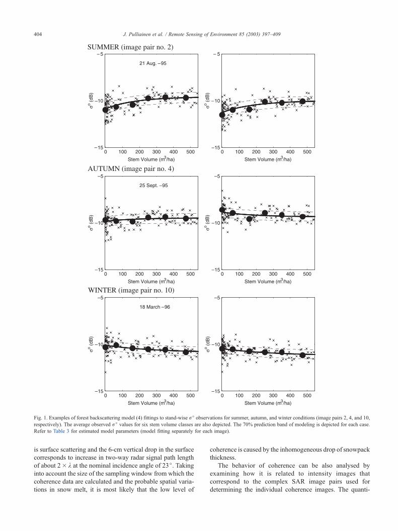
Table 3. Additionally, Fig. 1 demonstrates how well the

backscattering model fittings according to Eq. (8) agree with

the experimental observations under typical summer,

autumn, and winter conditions. Even though the fluctuations

of stand-wise observations from modeled curves are high,

the average level of backscatter for different stem volume

classes is well described by model (4). Note that the listed

and depicted rj values determined from ERS SLC images

show systematically lower values than those obtained from

ERS PRI images. This is due to the difference in the

calibration constant of these two image data.

As the coherence data and model (5) describe the

interferometric coherence as a function of forest stem

volume (biomass), the obtained results also enable the

quantitative study of the matter on how largely the image

acquisition conditions affect the level of coherence, separat-

ing the contribution of ground and that of forest canopy

Table 2

Forest stand characteristics

All 210

stands

134 stands larger than 1.5 ha

(85.4% of the total area)

Mean stem volume (m3/ha) 155.5 174.4

Std. of stem volume (m3/ha) 160.3 176.1

Minimum stem volume (m3/ha) 0 0

Maximum stem volume (m3/ha) 539.3 539.3

Mean stand area (ha) 2.4 3.2

Std. of stand area (ha) 1.9 1.9

Minimum stand area (ha) 0.2 1.52

Maximum stand area (ha) 13.8 13.8


(vegetation layer). The estimated model parameters c0,k and

c1,k directly describe the coherence of ground layer and

vegetation, respectively, for each image pair k.

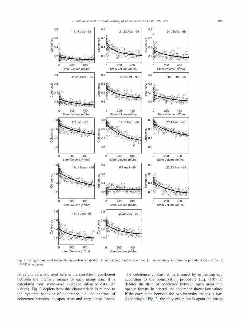
Fig. 2 shows the modeled behavior of coherence as well

as the actual stand-wise observations for all 14 INSAR

images. Also, the 70% prediction band of coherence mod-

eling is depicted for each case. The corresponding correla-

tion coefficients between the modeled coherence and

observed coherence are summarized in Table 4. The corre-

lation coefficients obtained between the data and model (7)

are also shown. The results in Table 4 confirm the con-

clusions of earlier investigations by indicating a high

temporal variability in correlation between the coherence

observations and stem volume, see, e.g. Fransson et al.

(2001), Koskinen et al. (2001), and Santoro et al. (2002).

According to Table 4, the model given by Eq. (5) describes

the behavior of interferometric coherence at the stand level

with a higher correlation than the model given by Eq. (7)

including the complex term. The lower correlation obtained

by model (7) is possibly caused by the inhomogeneity of

tree height inside individual forest stands.

Fig. 2 clearly indicates that the response of coherence to

increase in stem volume is nonlinear. This nonlinear behav-

ior is well described by the empirical models (4) and (5)

even though the scatter from the modeled (average) curve is

quite high at stand level.

4.2. Influence of weather-related factors on coherence

Fig. 2 indicates that the level of coherence is highly

dependent on seasonal conditions. The evident factors

affecting the level of coherence, and thereby parameters

c0,k and c1,k include the change in vegetation and soil/snow

moisture between the repeat pass SAR image acquisitions

and wind-induced changes in scatterer positions (absolute

positions of needles, branches, and tree tops). These aspects

can be investigated by analyzing the correlation between the

estimated model parameters (c0,k and c1,k) and weather

station observations-based indicators. The following quan-

titative indicators that are directly related either to changes

in vegetation and soil moisture conditions or changes in

(volume) scatterer positions are used here: (i) integrated

amount of precipitation between the moments of image pair

acquisition and (ii) averaged wind speed at about the

moments of image acquisition (refer to Table 1). The change

in temperature is used as a qualitative indicator as it is

essential especially when the temperature has varied above

and below the freezing point.

According to Fig. 2 and Table 4, the interferometric

coherence shows a low level, and consequently, has a low

correlation to biomass in five of the investigated images

(image pair nos. 1, 3, 4, 6, and 11). The precipitation andwind

speed data listed in Table 1 explain this behavior adequately

in four of the cases. In 17–18 July 1995 and 9–10 September

1995 (image pair nos. 1 and 3), considerable precipitation

occurred between the image acquisitions evidently causing

changes in the dielectric properties of the scene. For 25–26

September 1995 (image pair no. 4), the wind speed was high.

In the case of image pair no. 6, temperature was above the

freezing point in October 30 but below the freezing point in

October 31. This may have caused considerable changes in

the dielectric characteristics of the scene (refer to Table 3 for

backscattering model parameter values), which as well

decreases the overall level of coherence.

In one of the investigated interferometric images, the

image pair obtained for 6–7 April 1996 (image pair no.

11), the low level of coherence is not explained by the

temperature or precipitation behavior. During this image pair

acquisition, the scene was fully covered by wet snow.

Typically, the interferometric images obtained under snow-

covered conditions show very high coherence values. The

most probable reason decreasing the level of coherence for

the image pair no. 11 is the rapid melt of snow. The thickness

of the snowpack dropped about 6 cm between the image

acquisitions. As the drop in the snowpack thickness is a

spatially inhomogeneous phenomenon in a rugged forested

terrain (even at a small scale), it is possible that the low level

of coherence is directly caused by the snow melt: the

dominant backscattering mechanism from a wet snow layer

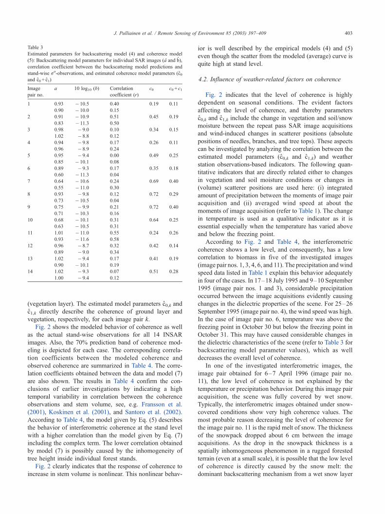
Table 3

Estimated parameters for backscattering model (4) and coherence model

(5): Backscattering model parameters for individual SAR images (a and b),

correlation coefficient between the backscattering model predictions and

stand-wise ro-observations, and estimated coherence model parameters (c0and c0 + c1)

Image

pair no.

a 10 log10 (b) Correlation

coefficient (r)

c0 c0 + c1

1 0.93 � 10.5 0.40 0.19 0.11

0.90 � 10.0 0.15

2 0.91 � 10.9 0.51 0.45 0.19

0.83 � 11.3 0.50

3 0.98 � 9.0 0.10 0.34 0.15

1.02 � 8.8 0.12

4 0.94 � 9.8 0.17 0.26 0.11

0.96 � 8.9 0.24

5 0.95 � 9.4 0.00 0.49 0.25

0.85 � 10.1 0.08

6 0.89 � 9.3 0.17 0.35 0.18

0.60 � 11.3 0.04

7 0.64 � 10.6 0.24 0.69 0.40

0.55 � 11.0 0.30

8 0.93 � 9.8 0.12 0.72 0.29

0.73 � 10.5 0.04

9 0.75 � 9.9 0.21 0.72 0.40

0.71 � 10.3 0.16

10 0.68 � 10.1 0.31 0.64 0.25

0.63 � 10.5 0.31

11 1.01 � 11.0 0.55 0.24 0.26

0.93 � 11.6 0.58

12 0.96 � 8.7 0.32 0.42 0.14

0.89 � 9.0 0.34

13 1.02 � 9.4 0.17 0.41 0.19

0.90 � 10.1 0.19

14 1.02 � 9.3 0.07 0.51 0.28

1.00 � 9.4 0.12


is surface scattering and the 6-cm vertical drop in the surface

corresponds to increase in two-way radar signal path length

of about 2� k at the nominal incidence angle of 23j. Takinginto account the size of the sampling window from which the

coherence data are calculated and the probable spatial varia-

tions in snow melt, it is most likely that the low level of

coherence is caused by the inhomogeneous drop of snowpack

thickness.

The behavior of coherence can be also analysed by

examining how it is related to intensity images that

correspond to the complex SAR image pairs used for

determining the individual coherence images. The quanti-

Fig. 1. Examples of forest backscattering model (4) fittings to stand-wise rj observations for summer, autumn, and winter conditions (image pairs 2, 4, and 10,

respectively). The average observed rj values for six stem volume classes are also depicted. The 70% prediction band of modeling is depicted for each case.

Refer to Table 3 for estimated model parameters (model fitting separately for each image).


tative characteristic used here is the correlation coefficient

between the intensity images of each image pair. It is

calculated from stand-wise averaged intensity data (rjvalues). Fig. 3 depicts how this characteristic is related to

the dynamic behavior of coherence, i.e. the contrast of

coherence between the open areas and very dense forests.

The coherence contrast is determined by estimating c1,kaccording to the optimization procedure (Eq. (10)). It

defines the drop of coherence between open areas and

opaque forests. In general, the coherence shows low values

if the correlation between the two intensity images is low.

According to Fig. 3, the only exception is again the image

Fig. 2. Fitting of empirical backscattering–coherence models (4) and (5) into stand-wise rj and AcA observations according to procedures (6)– (8) for 14

INSAR image pairs.


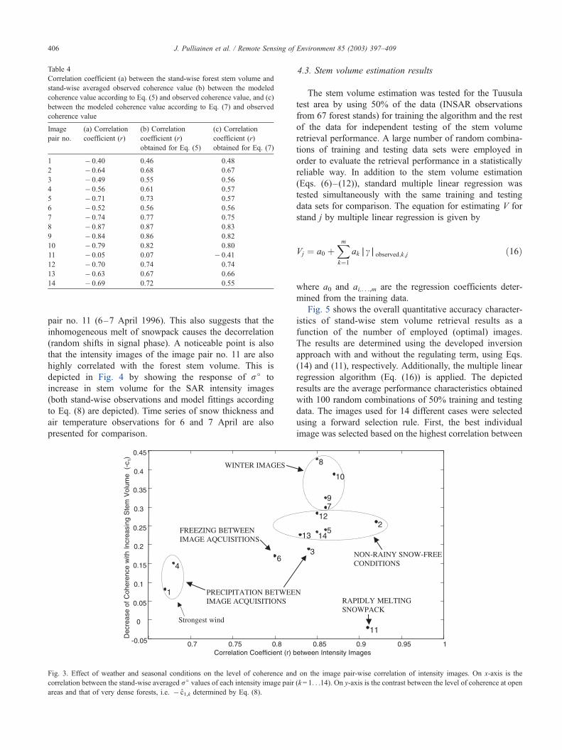
pair no. 11 (6–7 April 1996). This also suggests that the

inhomogeneous melt of snowpack causes the decorrelation

(random shifts in signal phase). A noticeable point is also

that the intensity images of the image pair no. 11 are also

highly correlated with the forest stem volume. This is

depicted in Fig. 4 by showing the response of rj to

increase in stem volume for the SAR intensity images

(both stand-wise observations and model fittings according

to Eq. (8) are depicted). Time series of snow thickness and

air temperature observations for 6 and 7 April are also

presented for comparison.

4.3. Stem volume estimation results

The stem volume estimation was tested for the Tuusula

test area by using 50% of the data (INSAR observations

from 67 forest stands) for training the algorithm and the rest

of the data for independent testing of the stem volume

retrieval performance. A large number of random combina-

tions of training and testing data sets were employed in

order to evaluate the retrieval performance in a statistically

reliable way. In addition to the stem volume estimation

(Eqs. (6)–(12)), standard multiple linear regression was

tested simultaneously with the same training and testing

data sets for comparison. The equation for estimating V for

stand j by multiple linear regression is given by

Vj ¼ a0 þXmk¼1

akAcAobserved;k;j ð16Þ

where a0 and ai,. . .,m are the regression coefficients deter-

mined from the training data.

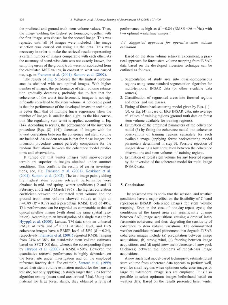
Fig. 5 shows the overall quantitative accuracy character-

istics of stand-wise stem volume retrieval results as a

function of the number of employed (optimal) images.

The results are determined using the developed inversion

approach with and without the regulating term, using Eqs.

(14) and (11), respectively. Additionally, the multiple linear

regression algorithm (Eq. (16)) is applied. The depicted

results are the average performance characteristics obtained

with 100 random combinations of 50% training and testing

data. The images used for 14 different cases were selected

using a forward selection rule. First, the best individual

image was selected based on the highest correlation between

Table 4

Correlation coefficient (a) between the stand-wise forest stem volume and

stand-wise averaged observed coherence value (b) between the modeled

coherence value according to Eq. (5) and observed coherence value, and (c)

between the modeled coherence value according to Eq. (7) and observed

coherence value

Image

pair no.

(a) Correlation

coefficient (r)

(b) Correlation

coefficient (r)

obtained for Eq. (5)

(c) Correlation

coefficient (r)

obtained for Eq. (7)

1 � 0.40 0.46 0.48

2 � 0.64 0.68 0.67

3 � 0.49 0.55 0.56

4 � 0.56 0.61 0.57

5 � 0.71 0.73 0.57

6 � 0.52 0.56 0.56

7 � 0.74 0.77 0.75

8 � 0.87 0.87 0.83

9 � 0.84 0.86 0.82

10 � 0.79 0.82 0.80

11 � 0.05 0.07 � 0.41

12 � 0.70 0.74 0.74

13 � 0.63 0.67 0.66

14 � 0.69 0.72 0.55

Fig. 3. Effect of weather and seasonal conditions on the level of coherence and on the image pair-wise correlation of intensity images. On x-axis is the

correlation between the stand-wise averaged rj values of each intensity image pair (k= 1. . .14). On y-axis is the contrast between the level of coherence at open

areas and that of very dense forests, i.e. � c1,k determined by Eq. (8).


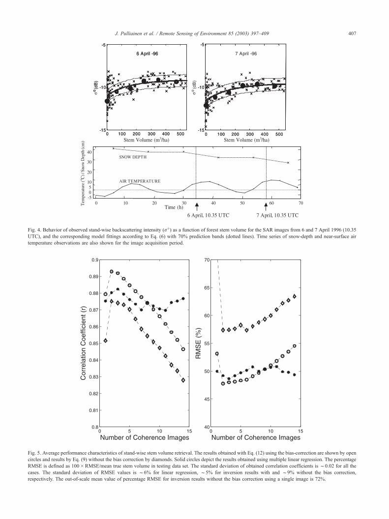
Fig. 4. Behavior of observed stand-wise backscattering intensity (rj) as a function of forest stem volume for the SAR images from 6 and 7 April 1996 (10.35

UTC), and the corresponding model fittings according to Eq. (6) with 70% prediction bands (dotted lines). Time series of snow-depth and near-surface air

temperature observations are also shown for the image acquisition period.

Fig. 5. Average performance characteristics of stand-wise stem volume retrieval. The results obtained with Eq. (12) using the bias-correction are shown by open

circles and results by Eq. (9) without the bias correction by diamonds. Solid circles depict the results obtained using multiple linear regression. The percentage

RMSE is defined as 100�RMSE/mean true stem volume in testing data set. The standard deviation of obtained correlation coefficients is f0.02 for all the

cases. The standard deviation of RMSE values is f6% for linear regression, f5% for inversion results with and f9% without the bias correction,

respectively. The out-of-scale mean value of percentage RMSE for inversion results without the bias correction using a single image is 72%.


the predicted and ground truth stem volume values. Then,

the image yielding the highest performance, together with

the first image, was chosen for the second image. This was

repeated until all 14 images were included. The image

selection was carried out using all the data. This was

necessary in order to make the retrieval results representing

a certain number of images comparable with each other. As

the accuracy of stand-wise data was not exactly known, the

sampling errors of the ground truth were not subtracted from

the calculated MSE values, in contrast to what was carried

out, e.g. in Fransson et al. (2001), Santoro et al. (2002).

The results of Fig. 5 indicate that the highest perform-

ance is obtained with two optimal images. With higher

number of images, the performance of stem volume estima-

tion gradually decreases, probably due to fact that the

coherence of the worst interferometric images is not sig-

nificantly correlated to the stem volume. A noticeable point

is that the performance of the developed inversion technique

is better than that of multiple linear regression when the

number of images is smaller than eight, as the bias correc-

tion (the regulating sum term) is applied according to Eq.

(14). According to results, the performance of the inversion

procedure (Eqs. (8)–(14)) decreases if images with the

lowest correlation between the coherence and stem volume

are included. An evident reason is that for those images, the

inversion procedure cannot perfectly compensate for the

random fluctuations between the coherence model predic-

tions and observations.

It turned out that winter images with snow-covered

terrain are superior to images obtained under summer

conditions. This confirms the results of earlier investiga-

tions, see, e.g. Fransson et al. (2001), Koskinen et al.

(2001), Santoro et al. (2002). The two image pairs yielding

the highest stem volume retrieval performance were

obtained in mid- and spring–winter conditions (12 and 13

February, and 2 and 3 March 1996). The highest correlation

coefficient between the estimated stem volume and the

ground truth stem volume showed values as high as

r = 0.89 (R2 = 0.79) and a percentage RMSE level of 48%.

This performance can be regarded as comparable to that of

optical satellite images (with about the same spatial reso-

lution). According to an investigation of a single test site by

Hyyppa et al. (2000), Landsat TM data show an unbiased

RMSE of 56% and R2 = 0.31 at stand level, and ERS

coherence images have a RMSE level of 58% (R2 = 0.24),

respectively. Fransson et al. (2001) reported RMSE ranging

from 24% to 38% for stand-wise stem volume estimates

based on SPOT XS data, whereas the corresponding figure

by Hyyppa et al. (2000) is RMSE = 50%. However, the

quantitative retrieval performance is highly dependent on

the forest site under investigation and on the employed

reference forestry data. For example, Santoro et al. (1999)

tested their stem volume estimation method for the Tuusula

test site, but only applying 18 stands larger than 2 ha for the

algorithm testing (mean stand area around 7 ha). Using that

material for large forest stands, they obtained a retrieval

performance as high as R2 = 0.84 (RMSE = 86 m3/ha) with

two optimal wintertime images.

4.4. Suggested approach for operative stem volume

estimation

Based on the stem volume retrieval experiment, a prac-

tical approach for forest stem volume mapping from INSAR

data based on the developed inversion technique can be

outlined as follows.

1. Segmentation of study area into quasi-homogeneous

regions using some standard segmentation algorithm for

multi-temporal INSAR data (or other available data

sources).

2. Classification of segmented areas into forested regions

and other land use classes.

3. Fitting of forest backscattering model given by Eqs. (1)–

(3), or Eq. (4) in case of ERS INSAR data, into average

rj values of training regions (ground truth data on forest

stem volume available for training regions).

4. Estimation of the empirical parameters of the coherence

model (5) by fitting the coherence model into coherence

observations of training regions separately for each

available image (applying forest backscattering model

parameters determined in step 3). Possible rejection of

images showing a low correlation between the coherence

observations and stem volumes of training regions.

5. Estimation of forest stem volume for any forested region

by the inversion of the coherence model for multi-image

INSAR data.

5. Conclusions

The presented results show that the seasonal and weather

conditions have a major effect on the feasibility of C-band

repeat-pass INSAR coherence images for stem volume

mapping. Even in the case of one-day-repeat cycle, the

conditions at the target area can significantly change

between SAR image acquisitions causing a drop of inter-

ferometric coherence, and thus, degrading the sensitivity of

coherence to stem volume variations. The demonstrated

weather conditions-related phenomena that degrade INSAR

coherence images include (a) precipitation between image

acquisitions, (b) strong wind, (c) freezing between image

acquisitions, and (d) rapid snow melt (decrease of snowpack

thickness) between the moments of repeat-pass image

acquisitions.

A new analytical model-based technique to estimate forest

stem volume from coherence data appears to perform well,

even for small regions when optimum coherence images or

large multi-temporal image sets are employed. It is also

possible to select optimum images beforehand based on

weather data. Based on the results presented here, winter


images with dry snow cover (temperatures well below the

freezing point) are always applicable for stem volume re-

trieval in boreal forests. In contrast to SAR intensity images,

coherence images obtained under wet snow conditions are, at

least occasionally, totally unusable for stem volume (or bio-

mass) mapping. The obtained stem volume retrieval perform-

ance was close to that of optical satellite images.

References

Askne, J., Dammert, P., Ulander, L., & Smith, G. (1997). C-band repeat-

pass interferometric SAR observations of the forest. IEEE Transactions

on Geoscience and Remote Sensing, 35, 25–35.

Askne, J., Santoro, M., Smith, G., & Fransson, J. (2002). Large area boreal

forest investigations using ERS INSAR. Proc. 3rd Int. Symp. Retrieval

of Bio- and Geophysical Parameters from SAR Data for Land Applica-

tions, ESA SP-475, Sheffield, UK 11–14 September 2001 ( pp. 39–44).

The Netherlands: ESA Publications Division, Noordwijk.

Fransson, J., Smith, G., Askne, J., & Olsson, H. (2001). Stem volume esti-

mation in boreal forests using ERS-1/2 coherence and SPOT XS optical

data. International Journal of Remote Sensing, 21(14), 2777–2791.

Gatelli, F., Monti Guarnieri, A., Parizzi, F., Pasquali, P., Prati, C., & Rocca,

F. (1994). The wavenumber shift in SAR interferometry. IEEE Trans-

actions on Geoscience and Remote, 32.

Hyyppa, J., Hyyppa, H., Inkinen, M., Engdahl, M., Linko, S., & Zhu, Y.-H.

(2000). Accuracy comparison of various remote sensing data sources in

the retrieval of forest stand attributes. Forest Ecology and Management,

128, 109–120.

Koskinen, J., Pulliainen, J., Hyyppa, J., Engdahl, M., & Hallikainen, M.

(2001). The seasonal behavior of interferometric coherence in boreal

forest. IEEE Transactions on Geoscience and Remote Sensing, 39,

820–829.

Laur, H., Bally, P., Meadows, P., Sanchez, J., Schaettler, B., & Lopinto, E.

(1997). Derivation of backscattering coefficient rj in ESA ERS SAR

PRI products. (ESA ESRIN, ES-TN-RS-PM-HL09, Issue 2, Rev. 4).

Lee, J. (1981). Speckle analysis and smoothing of synthetic aperture radar

images. Computer Graphics and Image Processing, 17, 24–32.

Lehtinen, M. (1988). On statistical inversion theory. Pitman Research

Notes in Mathematics Series, 167, 46–57.

Lopes, A., Nezry, E., Touzi, R., & Laur, H. (1993). Structure detection and

statistical adaptive filtering in SAR images. International Journal of

Remote Sensing, 14(9), 1735–1758.

Pulliainen, J., Heiska, K., Hyyppa, J., & Hallikainen, M. (1994). Back-

scattering properties of boreal forests at the C- and X-band. IEEE Trans-

actions on Geoscience and Remote Sensing, 32, 1041–1050.

Pulliainen, J., Kurvonen, L., & Hallikainen, M. (1999). Multi-temporal

behavior of L- and C-band SAR observations of boreal forests. IEEE

Transactions on Geoscience and Remote Sensing, 37, 927–937.

Pulliainen, J., Mikkela, P., Hallikainen, M., & Ikonen, J.-P. (1996). Seasonal

dynamics of C-band backscatter of boreal forests with applications to

biomass and soil moisture estimation. IEEE Transactions on Geoscience

and Remote Sensing, 34, 758–770.

Quegan, S., Le Toan, T., Yu, J., Ribbles, F., & Floury, N. (2000). Multi-

temporal ERS SAR analysis applied to forest mapping. IEEE Trans-

actions on Geoscience and Remote Sensing, 38, 741–753.

Quegan, S., & Yu, J. (2001). Filtering of multichannel SAR images. IEEE

Transactions on Geoscience and Remote Sensing, 39, 2373–2379.

Santoro, M., Askne, J., Dammert, P., Fransson, J., & Smith, G. (1999).

Retrieval of biomass in boreal forest from multi-temporal ERS-1/2 in-

terferometry. Proc. FRINGE’99, ESA SP-478, Liege, Belgium, 10–12

Nov. 1999.

Santoro, M., Askne, J., Smith, G., & Fransson, E. (2002). Stem volume

retrieval in boreal forest from ERS-1/2 interferometry. Remote Sensing

of Environment, 81, 19–35.

Treuhaft, R., & Siquira, P. (2000). Vertical structure of vegetated land

surfaces from interferometric and polarimetric radar. Radio Science,

35, 141–177.

Wagner, W., Vietmeier, J., Schmullius, C., Davidson, M., Le Toan, T.,

Quegan, S., Yu, J., Luchman, A., Tansey, K., Balzter, H., & Gaveau,

D. (2000). The use of coherence from ERS Tandem pairs for determin-

ing forest stock volume in SIBERIA. Proc. IGARSS’00, Honolulu,

USA, 24–28 July 2000 ( pp. 1396–1398). NJ: IEEE Piscataway.

Wegmuller, U., Werner, C., & Strozzi, T. (1998). SAR interferometric and

differential interferometric processing chain. Proc. IGARSS’98, 2, Seat-

tle, USA, 6–10 July 1998 ( pp. 1106–1108). NJ: IEEE Piscataway.

Zebker, H., & Villasenor, J. (1992). Decorrelation in interferometric radar

echoes. IEEE Transactions on Geoscience and Remote Sensing, 30,

950–959.


Feasibility of multi-temporal interferometric SAR data for stand-level estimation of boreal forest...

Documents

Transcript of Feasibility of multi-temporal interferometric SAR data for stand-level estimation of boreal forest...