Facet evolution on supported nanostructures: Effect of finite height

Pak-Wing Fok,1,2 Rodolfo R. Rosales,3 and Dionisios Margetis4

1Applied and Computational Mathematics, California Institute of Technology, Pasadena, California 91125, USA2Department of Biomathematics, University of California–Los Angeles, Los Angeles, California 90095, USA3Department of Mathematics, Massachusetts Institute of Technology, Cambridge, Massachusetts 02139, USA

4Department of Mathematics and Institute for Physical Science and Technology, University of Maryland, College Park,Maryland 20742, USA

�Received 15 April 2008; revised manuscript received 30 September 2008; published 1 December 2008�

The surface of a nanostructure relaxing on a substrate consists of a finite number of interacting steps andoften involves the expansion of facets. Prior theoretical studies of facet evolution have focused on models withan infinite number of steps, which neglect edge effects caused by the presence of the substrate. By consideringdiffusion of adsorbed atoms �adatoms� on terraces and attachment-detachment of atoms at steps, we show thatthese edge or finite height effects play an important role in the structure’s macroscopic evolution. We assumediffusion-limited kinetics for adatoms and a homoepitaxial substrate. Specifically, using data from step simu-lations and a continuum theory, we demonstrate a switch in the time behavior of geometric quantities associ-ated with facets: the facet edge position in a straight-step system and the facet radius of an axisymmetricstructure. Our analysis and numerical simulations focus on two corresponding model systems where steps repeleach other through entropic and elastic dipolar interactions. The first model is a vicinal surface consisting of afinite number of straight steps; for an initially uniform step train, the slope of the surface evolves symmetricallyabout the centerline, i.e., the middle step when the number of steps is odd. The second model is an axisym-metric structure consisting of a finite number of circular steps; in this case, we include curvature effects whichcause steps to collapse under the effect of line tension. In the first case, we show that the position of the facetedge, measured from the centerline, switches from O�t1/4� behavior to O�t1/5� �where t is time�. In the secondcase, the facet radius switches from O�t1/4� to O�t�. For the axisymmetric case, we also predict analyticallythrough a continuum shock wave theory how the individual collapse times are modified by the effects of finiteheight under the assumption that step interactions are weak compared to the step line tension.

DOI: 10.1103/PhysRevB.78.235401 PACS number�s�: 81.15.Aa, 81.10.�h, 68.55.J�

I. INTRODUCTION

Understanding the fundamental properties of small sup-ported crystal mounds is important for applications incatalysis1 and nanoparticle growth.2 However, characterizingthe morphology of nanoscale structures is still a challengingproblem and our ability to control their evolution is fairlylimited.3

As fabricated structures become smaller, finite-size effectsassociated with the crystal’s geometry become more impor-tant. The steps that bound each monolayer in the structureare usually closed and have a finite radius of curvature. As aresult, in the absence of material deposition, the perimeter ofa single isolated step generally shrinks—a phenomenon thatis well understood in terms of a step line tension.4,5 In addi-tion to step curvature, another quantity that is clearly finite isthe number of monolayers that make up the nanostructure.However, the effects of finite height have received much lessattention in theoretical treatments compared to infinite andperiodic surface features. �An infinite surface feature is onethat has an infinite number of monolayers.� Furthermore, themain results to date apply only to crystals at equilibrium,where there is no facet motion. The combined effect of finiteheight and facet evolution remains unexplored.

For crystal surfaces undergoing relaxation below theroughening transition temperature, facets expand due to thesequential collapse of extremal steps under the influence ofline tension.5,6 �An extremal step is one that has only one

neighboring step.� For axisymmetric structures with a �circu-lar� facet, scaling laws of the form r�t�=O�t�� are oftenobserved.2,7–9 Here, r�t� is the facet radius, t is time, and theexponent � depends on the initial structure’s shape and thedominant transport process.2,10 However, theoretical deriva-tions of these scaling laws ignore the effect of the substrateand are therefore valid only for infinite structures. On theother hand, most studies of supported finite structures as-sume an equilibrium shape under which facet motion is ab-sent altogether.11–14

In this paper, we study the facet evolution of crystal struc-tures relaxing toward planarity when the number of steps isfinite. Our models are based on the Burton-Cabrera-Frank�BCF� theory15 for vicinal surfaces. The key microscopicprocesses involve adsorbed atoms �“adatoms”� diffusing onterraces between steps and atoms attaching to and detachingfrom step edges. By balancing the flux of adatoms in and outof each step edge, one can write down equations of motion todescribe the morphological evolution of the vicinal surface.Two commonly studied step geometries are the straight-stepmodel16,17 and the axisymmetric model8,9,18 �see Fig. 1�. Ourmain results show that very different scaling properties arisewhen only a finite number of steps are present in the struc-ture. In particular, for a set of infinitely long straight stepsthat are initially uniformly spaced and separate semi-infinitefacets, the step positions evolve symmetrically with respectto the centerline �an assumed axis of symmetry� �see Fig.1�a��. The scaling with time for the position of each facetedge, measured from the centerline, switches from O�t1/4� to

PHYSICAL REVIEW B 78, 235401 �2008�

1098-0121/2008/78�23�/235401�17� ©2008 The American Physical Society235401-1

O�t1/5� when finite height effects become important. In themore physically relevant case of concentric circular stepssurrounding a facet �see Fig. 1�b��, the analogous result isthat the scaling for the facet radius switches from r�t�=O�t1/4� to O�t�. To our knowledge, these switches in thetime behavior have neither been reported nor studied before.We show these results by first numerically solving the equa-tions of motion for a finite set of discrete steps. Then, wevalidate the numerical data and the scaling laws by setting upand solving a nonlinear partial differential equation �PDE�for each geometry. Interestingly, our numerical data for cir-cular steps suggest that the ratio of the step-step interactionenergy to the step line tension can be estimated by measuringthe step collapse times.

When modeling the effect of the substrate, we assume thatthe nanostructure and its substrate are made up of the samematerial and that any lattice mismatch between the substrateand the crystal is small enough to be considered as negli-gible. Hence, the effects of mismatch-induced stress are ig-nored, and the base step acts as a perfect sink for all diffus-ing adatoms. As a result, the surface relaxation conservesvolume in the axisymmetric model. Therefore the finiteheight effects studied in this paper are associated with geo-metric constraints inherent in the relaxation. Finally, themass transport process on the structure’s surface is alwaysassumed to be terrace diffusion limited. The cases withattachment-detachment and edge-diffusion-limited kinetics,although important, complicate the analysis and lie beyondthe scope of this paper.

Of the two model systems studied in this paper �see Fig.1�, the axisymmetric configuration of steps is more physi-cally relevant because: �i� steps in experiments are usually

closed and �ii� the effect of step line tension is taken intoaccount. Although steps are never perfectly circular, there aremany experiments where relaxing nanostructures are wellapproximated as being axisymmetric.5,7,19,20 Our results forthe straight-step system should be applicable to the specialsituations where step line tension is unimportant. This sys-tem can perhaps be thought of as a model for a set of stepsthat evolves from a “step bunch” initial configuration. In thiscase, the width of the terraces separating the bunches is largecompared to the interstep distance �inside the bunches�, sothat each bunch evolves in isolation at least initially.

The layout of the remainder of this paper is as follows.Section II focuses on the discrete step equations �coupleddifferential equations� in the straight step or one-dimensional�1D� and axisymmetric cases. For each type of geometry, wederive the governing equations of motion for a finite collec-tion of steps and solve these equations numerically. In Sec.III, we use continuum models to find scaling laws for facetevolution in the 1D and axisymmetric settings. In particular,for the axisymmetric case, we use Lagrangian coordinates todevelop a shock wave theory for facet evolution. We validatethe scaling laws and the shock wave theory using numericalresults from Sec. II. In Sec. IV, we conclude our paper witha discussion of our results.

II. STEP EQUATIONS OF MOTION

Before deriving the step equations of motion, we motivatethe study of our two model systems, which are illustrated inFig. 1. Although geometrically simple, these models capturethe essential features in the time behavior of finite surfacestructures. We expect that results for these relatively simplemodels should carry over to more general geometries, atleast at a qualitative level. In Fig. 1�a�, the straight-stepmodel is also worth studying in its own right because, as wewill show, it has a simple analytic solution that is in exactagreement with step simulation data.

The ideas developed in the straight-step model can beused to understand the more physically relevant axisymmet-ric case, illustrated in Fig. 1�b�. For this system, a facet de-velops and evolves at the top of the nanostructure as theinnermost steps collapse.

We now state in more details the assumptions we make inorder to set up the discrete step equations of motion for thetwo geometries in Fig. 1. These assumptions can be broadlydivided into two categories: those that relate to the “interiorsteps,” i.e., non-extremal steps, and those that relate to theinterface between the nanostructure and the substrate orfacet.

First let us consider the assumptions we make for thenanostructure itself. We assume that the surface relaxes inthe absence of deposition and desorption. Furthermore, theadatom diffusion on terraces is the rate-limiting �slowest�process, with the attachment-detachment of atoms at stepedges being relatively fast. We assume that no other facetsdevelop throughout the entire course of the surface evolu-tion.

Next, we consider the assumptions involved when model-ing the effect that the substrate has on the structure’s relax-

FIG. 1. The two model systems studied in this paper. �a� A finitenumber of straight steps separating two semi-infinite �flat� facets,possibly representing a straight-step bunch. Facet edges, w1�t� andw2�t�, are measured from the centerline. �b� A finite number ofcircular steps, representing an axisymmetric nanostructure. A mac-roscopic facet, with radius r�t�, develops at the top of the structureas innermost steps collapse.

FOK, ROSALES, AND MARGETIS PHYSICAL REVIEW B 78, 235401 �2008�

235401-2

ation. The most important assumption is that we neglect theeffect of stress caused by the lattice mismatch between thesupported crystal and the substrate,21 considering this to besufficiently small. In the straight-step model �Fig. 1�a��, weset the adatom flux to be zero on both facets. In the axisym-metric case �see Fig. 1�b��, we set this flux to be zero on thesubstrate; this condition is equivalent to conserving the nano-structure’s volume.

For the 1D case, we let the dimensional positions of thestep edges be xi�t�, i=1,2 , . . . ,N where t is dimensionaltime. We define the terrace i to be the region xi�x�xi+1between steps i and i+1; facets are the regions xN� x��and −�� x� x1. Furthermore, the evolution of the surfacepreserves the symmetry of the profile about x�N+1�/2 if N isodd and about �xN/2+ xN/2+1� /2 if N is even: the facets arealways mirror images of each other.

For the axisymmetric case, we let ri�t� describe the �di-mensional� radius of each circular step, with the substratebeing identified with the region rN� r��. In contrast to thestraight-step case, the faceted region is not 0� r� r1. In fact,we will see in Sec. III B that, when the top step is about tocollapse, the faceted region can be described fairly well by0� r� r2. �In particular, we refer the reader to Fig. 8�a� ofSec. III B for an illustration of this point.�

Broadly speaking, the facet is a macroscopic object. Itsstrict definition rests on the assumed behavior of the stepdensity �positive surface slope� at the facet edge within thecontinuum theory, as discussed in Sec. III.

A. Straight steps

We now briefly derive the equations of motion for N in-finitely long straight steps using a BCF-type model.15 Con-sider a monotonic step train with N descending steps. Bymass conservation, the step velocity is

dxi

dt=

�

a�Ji−1�xi� − Ji�xi�� , �1�

where � is the atomic volume, a is the step height, xi�t� isthe step position as a function of time t, and Ji is the adatomflux defined by Ji=−D

�ci

�x , where D is the terrace diffusivity, xis the Cartesian coordinate, and ci�x� is the adatom concen-tration on terrace i. Under the quasi-steady approximation��tci�0�, ci�x� obeys

�2ci = 0, �2�

which has a solution ci�x�=Aix+Bi. The constants Ai and Biare found by enforcing boundary conditions for theattachment-detachment of adatoms at step edges

D� �ci

� x�

xi

= k�ci�xi− Ci

eq� , �3�

− D� �ci

� x�

xi+1

= k�ci�xi+1− Ci+1

eq � , �4�

where k is the attachment-detachment rate of adatoms at astep edge and we have assumed the absence of an Ehrlich-

Schwoebel barrier.22,23 In Eq. �3�, Cieq is the equilibrium ada-

tom concentration at the step edge given approximately by

Cieq � cs�1 +

�i

kBT . �5�

Here, �i is the step chemical potential at the ith step edge,kBT is the Boltzmann energy, and cs is the equilibrium ada-tom concentration at an isolated straight step. The stepchemical potential describes the propensity for a step edge toaccept adatoms. For entropic and/or elastic dipolar interac-tions, �i is given by24

�i

kBT= g� L

xi+1 − xi3

− � L

xi − xi+13� , �6�

where g is a dimensionless step-interaction coefficient and Lis the initial distance of separation between steps. Typically Lcan range from 10 to 104 Å.16,25 We now introduce the di-mensionless variables xi= xi /L and t= t / �D /k2�. Furthermore,we restrict ourselves to diffusion-limited kinetics so that forall i, D /kL� �xi+1−xi�, the dimensionless step separation.Note that the use of k in our time scale, D /k2, does not affectany dimensional results we derive since the dimensionalequations of motion �and initial data� do not depend on k.Then, Eq. �1� with Eqs. �2�–�6� becomes

dxi

dt= ���

1

xi+2 − xi+13

− 2� 1

xi+1 − xi3

+ � 1

xi − xi−13

�xi+1 − xi�

−� 1

xi+1 − xi3

− 2� 1

xi − xi−13

+ � 1

xi−1 − xi−23

�xi − xi−1� ,

�7�

where

� =cs�D2g

ak2L2 . �8�

Equation �7� is valid only when i=3,4 , . . . ,N−3, N−2.Steps 1, 2, N−1, and N obey different equations. For ex-ample, the motion of x1 and xN will be determined only bythe adatom fluxes on the first and �N−1�th terraces: underthe quasi-steady approximation, there can be no gradients inthe adatom concentration for x�x1 and xxN. Hence, we setJ0=JN=0, consistent with previous work.9 The step at x2 iscoupled to the steps at x1 and x3 through steady-state diffu-sion equations and their boundary conditions which involvethe step chemical potentials �1 and �3. However, �1 willonly couple together x1 and x2 in contrast to Eq. �6�. Simi-larly, step N only experiences “one-sided” interactions withstep N−1 and the equation for the velocity dxN−1 /dt must bemodified accordingly. Therefore, to supplement Eq. �7�, wehave the relations

FACET EVOLUTION ON SUPPORTED NANOSTRUCTURES:… PHYSICAL REVIEW B 78, 235401 �2008�

235401-3

dx1

dt= ���

1

x3 − x23

− 2� 1

x2 − x13

�x2 − x1� , �9�

dx2

dt= ���

1

x4 − x33

− 2� 1

x3 − x23

+ � 1

x2 − x13

�x3 − x2�

−� 1

x3 − x23

− 2� 1

x2 − x13

�x2 − x1� , �10�

dxN−1

dt= ��− 2� 1

xN − xN−13

+ � 1

xN−1 − xN−23

�xN − xN−1�

−� 1

xN − xN−13

− 2� 1

xN−1 − xN−23

+ � 1

xN−2 − xN−33

�xN−1 − xN−2� ,

�11�

dxN

dt= ��−

− 2� 1

xN − xN−13

+ � 1

xN−1 − xN−23

�xN − xN−1� . �12�

Equations �7� and �9�–�12�, with suitable initial data, com-pletely specify the motion of N straight steps moving underthe effect of entropic and/or elastic dipolar repulsions. Inte-grating these equations �with unit initial step separation�yields the curves in Fig. 2, where several snapshots areshown of the step density Fi�

1xi+1−xi

as a function of the stepposition xi. Note that at early times there is a maximum inthe step density near each of the extremal steps, while farfrom these steps the density is still approximately constant.

Finally, note that the form of Eqs. �9�–�12� is particular tothe physical situation being considered. In our case, the ex-tremal steps are free to move outward indefinitely withoutrestriction. This is not true in Ref. 17, for example: there, theequations of motion for steps 1, 2, N−1, and N are differentdue to step-antistep annihilations occurring at the peaks andvalleys of 1D periodic corrugations.

B. Circular steps

The derivation of the equations of motion for the axisym-metric case is similar to Sec. II A, but is slightly modified totake into account the effect of step line tension. We use Eq.�1� but with radial positions ri and r replacing xi and x. Theadatom fluxes Ji are induced by differences in the step edge

chemical potentials �i. In the axisymmetric case withdiffusion-limited kinetics the Ji take the form18

Ji�r, t� = −Dcs

kBT

1

r

�i+1 − �i

ln�ri+1/ri�. �13�

The two main differences between the straight and circular-step cases arise through the step interactions and step linetension. Both of these effects are encapsulated in the axisym-metric step chemical potential �i. Instead of Eq. �6�, we nowhave18

�i =�g1

ri

+�

2ari

��V�ri, ri+1� + V�ri−1, ri��� ri

. �14�

In Eq. �14�, g1 is the step line tension �a constant� andV�ri , ri+1� is the interaction potential between steps i and i+1. The first term, �g1 / ri, accounts for the curvature effectof each step. Assuming entropic and/or elastic dipolar repul-sions, V takes the form6

V�ri, ri+1� =4a3g3

3

riri+1

�ri + ri+1��ri+1 − ri+1�2 , �15�

where g3 is the step-interaction coefficient. From Eqs. �14�and �15�, we define a dimensionless parameter g�g3 /g1 toquantify the strength of the step-step interactions relative tothe step line tension. Analogous to the straight-step case, weset the adatom fluxes to be zero when r� r1 and r rN sothat J0=JN=0. Equations �1� and �13�–�15� with suitable ini-tial data for the step positions now completely specify themotion of all N steps in the nanostructure. In dimensionlessvariables, the governing equations are

−15 −10 −5 0 5 10 15

0.7

0.8

0.9

1

1.1

step position xi

step

dens

ityF

i

t=0t=5t=50t=100

FIG. 2. Simulation data for the �discrete� straight-step density Fi

as a function of the �scaled� step position xi. The profiles wereobtained by solving Eqs. �7� and �9�–�12� numerically with thenumber of steps N=31 and the dimensionless constant �defined inEq. �8�� �=1.

FOK, ROSALES, AND MARGETIS PHYSICAL REVIEW B 78, 235401 �2008�

235401-4

dr1

dt= −

�

r1�1

r1−

1

r2+ g� �0,r1,r2� − �r1,r2,r3��

ln�r2/r1� � , �16�

dr2

dt= −

�

r2�1

r2−

1

r3+ g� �r1,r2,r3� − �r2,r3,r4��

ln�r3/r2�−

1

r1−

1

r2+ g� �0,r1,r2� − �r1,r2,r3��

ln�r2/r1� � , �17�

dri

dt= −

�

ri�1

ri−

1

ri+1+ g� �ri−1,ri,ri+1� − �ri,ri+1,ri+2��

ln�ri+1/ri�−

1

ri−1−

1

ri+ g� �ri−2,ri−1,ri� − �ri−1,ri,ri+1��

ln�ri/ri−1� �,

i = 3,4, . . . ,N − 2, �18�

drN−1

dt= −

�

rN−1�1

rN−1−

1

rN+ g� �rN−2,rN−1,rN� − �rN−1,rN,���

ln�rN/rN−1�−

1

rN−2−

1

rN−1+ g� �rN−3,rN−2,rN−1� − �rN−2,rN−1,rN��

ln�rN−1/rN−2� � ,

�19�

drN

dt= +

�

rN�1

rN−1−

1

rN+ g� �rN−2,rN−1,rN� − �rN−1,rN,���

ln�rN/rN−1� � , �20�

where

�ri−1,ri,ri+1� =2ri+1

ri+1 + ri

1

�ri+1 − ri�3 −2ri−1

ri + ri−1

1

�ri − ri−1�3 +1

ri� ri+1

ri+1 + ri2 1

�ri+1 − ri�2� + � ri−1

ri + ri−12 1

�ri − ri−1�2� . �21�

Here r� r / l and t� t�D/k2� , where l is a length scale defined in

the next paragraph and g�l�= 23 �a / l�2�g3 /g1�. Again, the use

of k in the chosen time scale D /k2 does not affect any di-mensional results we derive. The prefactor ��l�= �

D2�2csg1

ak2kBT�l−3 is a dimensionless parameter that determines

the time scale of evolution. One can always choose timeunits so that �=1 as we do in our numerical calculations.

The length scale l could take one of two “natural” values.One choice is to take l=L, the initial step separation distance�initial terrace width�, analogous to the straight-step case.This is done to simulate experiments, in which case the steppositions are initialized to be rn=n, n=1,2 , . . . ,N. In oursimulations, we always take ��L�=1. Another possibility isto take l=Rc, the initial radius of the base step. This secondchoice is made in Sec. III B on Lagrangian theory. For futurereference, we note that ��L� /N3=��Rc� and g�L� /N2=g�Rc�.

Equations �16�–�21� for concentric circular steps have animportant difference from Eqs. �7� and �9�–�12� for straight

steps. Because of the step line tension, the radius of the topstep shrinks and undergoes a monotonic collapse, resulting ina successive “peeling” of the top layer.5,7 The removal of thetop layer reveals an underlying one that has a larger radius.5

Therefore, the facet evolution consists of a radial expansionalong with a downward translation. This evolution has beenstudied in the case of infinite axisymmetric structures: inparticular, for an equally spaced initial step configuration, wehave8,18,26 r�t�=O�t1/4� and h0−h�t�=O�t1/4� for t�1, wherer�t� is the facet radius, h�t� is the �dimensionless� verticallocation of the facet relative to some reference height h0, andt is �dimensionless� time.

Another interesting quantity to study is the collapse timeof the top step. These collapse times arise naturally in thesolution of Eqs. �16�–�20� and can be found fromexperiments.5,7,20 When we integrate Eqs. �16�–�20� numeri-cally and a collapse occurs, our convention is to remove thevariable corresponding to the innermost index, rj, for in-stance, and continue the integration with rj+1�t� as the inner-

FACET EVOLUTION ON SUPPORTED NANOSTRUCTURES:… PHYSICAL REVIEW B 78, 235401 �2008�

235401-5

most step. For example, after the first collapse, r1 is removedfrom the system and r2 obeys Eq. �16� but with r1→r2, r2→r3, and r3→r4. Likewise, r3 obeys Eq. �17� but with r1→r2, r2→r3, r3→r4, and r4→r5. Hence, throughout the en-tire course of the integration, a particular step index alwaysfollows the same step. The behavior of these collapse timesis crucial in determining the evolution �expansion� of thefacet. Qualitatively, if the steps collapse frequently, the facetevolution will proceed rather quickly. On the other hand, ifsteps do not collapse at all, the facet will remain frozen intime. Simple scaling results have been obtained for geometri-cally simple structures with a practically infinite number ofsteps.8 For collapse times tn, and n�1, we have tn=O�n4�when the spacing of steps is initially uniform �correspondingto cone shaped structures�. Other initial step spacings resultin different exponents.27

The scaling laws for the facet discussed above are inti-mately connected to the self-similarity inherent in the evolu-tion of infinite nanostructures.8,26,27 When the kinetics is dif-fusion limited and the number of steps approaches infinity,future height profiles of the nanostructure look like stretchedversions of past ones. This self-similarity is stable in thesense that small perturbations to an initial configuration ofequally spaced circular steps eventually decay.27

In the axisymmetric case, this self-similarity property isdestroyed with the onset of finite height effects. The reasonfor this is that the base step acts as the ultimate mass sink forthe adatom flux. As a result, the radii of the last few stepsgrow with time as mass is expelled from the top of the struc-ture and accumulates at the bottom. In this case, instead ofself-similarity in the height profile, we show below that scal-ing laws in the collapse times tn can be determined.

In general, the collapse times depend not only on the ini-tial values of the step radii, but on g as well. Thus, for astructure initially consisting of N concentric and equallyspaced circular steps, let tn�N ,g�, for n=1,2 ,3 , . . ., be thecollapse times. Furthermore, define the collapse time dis-crepancies with those of an infinite structure by

En�N,g� = tn�N,g� − tn��,g� . �22�

Figure 3�a� shows En�N ,0.01� plotted as a function of n forN=40, 50, and 60. Figure 3�b� shows that the step simulationdata collapse onto a single universal curve given by

G� n

N,g =

En�N,g�N4 . �23�

We note the following points about Eq. �23�. First, G is non-monotonic. In particular, the inset of Fig. 3�b� shows thepresence of a local maximum for n /N�0.45 before the mini-mum at n /N�0.76. Although not visible in the plots, thealternating pattern of minima and maxima continues forsmaller values of n /N, with the amplitudes decreasingquickly as n /N→0. Compared to an infinite structure, thestep collapse times for a finite structure occur earlier, thenlater, then earlier, etc. in an alternating fashion. For the datain Fig. 3�b�, we found that the positions of the first fourextrema �counting from the right� were at n /N�0.76, 0.45,0.33, and 0.25. We do not know if extrema exist for smaller

values of n /N. If they do, their amplitudes are too small forus to reliably detect these extrema. From the first four ex-trema, it appears that the spacing between them gets smalleras n /N gets smaller, with the amplitudes decreasing by aboutan order of magnitude from one extremum to the next. Sec-ond, relation �23� seems to hold for 0.25�n /N�1; forn /N�0.25, the collapse of data onto a single curve is lessclear because of numerical errors. These errors are on theorder of �or greater than� �G�, making it difficult to draw firmconclusions about the behavior of En�N ,g�. Third, from Fig.3�b�, G�·� appears to be a smooth continuous curve, at leastwhen 0.25�n /N�1. �For smaller values of n /N the evi-dence is again inconclusive for the same reason discussedabove.�

It seems reasonable to expect that a dependence such asEq. �23� should be derivable from a continuous model in thelarge N limit. In fact, we show that this is so in the zero-glimit in Sec. III B. Remarkably, even when N is as small as40, most of the collapse times seem to obey an underlyingcontinuum equation. Finally, since it is known that tn�� ,g�� t�n4 when n�1,8,26 for large n �and N� we have

0 20 40 60-1

-0.5

0

0.5

1

1.5

2x 10

5

n

En

N = 40N = 50N = 60

0 0.2 0.4 0.6 0.8 1-6

-4

-2

0

2

4

6

8

10

12

14

n/N

En/N

4

N = 40N = 50N = 60

0.35 0.4 0.45 0.5

20

10

0

(a)

(b)

FIG. 3. �a� Circular-step �radial case� simulation data for thescaled deviations En defined in Eq. �22� with the step-interactionparameter g=0.01. Step collapse times for an infinite structure,tn�� ,g�, were approximated with tn�N=700,g�. �b� The similaritycollapse data from �a� by Eq. �23�. Inset shows a local maximum ofEn /N4 for n /N�0.45.

FOK, ROSALES, AND MARGETIS PHYSICAL REVIEW B 78, 235401 �2008�

235401-6

tn�N ,g� /N4� G�n /N ,g�, where G�x ,g��G�x ,g�+ t��g�x4

and t� has been documented for a wide range of g values inRef. 26.

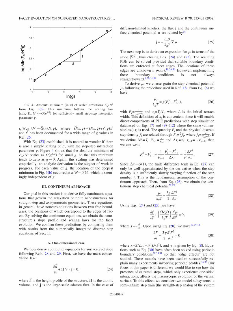
With Eq. �23� established, it is natural to wonder if thereis also a simple scaling of En with the step-step interactionparameter g. Figure 4 shows that the absolute minimum ofEn /N4 scales as O�g1/2� for small g, so that this minimumtends to zero as g→0. Again, this scaling was determinedempirically: an analytic derivation is the subject of work inprogress. For each value of g, the location of the deepestminimum in Fig. 3�b� occurred at n /N�0.76, which is seem-ingly independent of g.

III. CONTINUUM APPROACH

Our goal in this section is to derive fully continuum equa-tions that govern the relaxation of finite nanostructures forstraight-step and axisymmetric geometries. These equations,in general, have nonzero solutions between two free bound-aries, the positions of which correspond to the edges of fac-ets. By solving the continuum equations, we obtain the nano-structure’s slope profile and scaling laws for the facetevolution. We confirm these predictions by comparing themwith results from the numerically integrated discrete stepequations of Sec. II.

A. One-dimensional case

We now derive continuum equations for surface evolutionfollowing Refs. 28 and 29. First, we have the mass conser-vation law

� h

� t+ � � · j = 0, �24�

where h is the height profile of the structure, � is the atomicvolume, and j is the large-scale adatom flux. In the case of

diffusion-limited kinetics, the flux j and the continuum sur-face chemical potential � are related by18

j = −csD

kBT� � . �25�

The next step is to derive an expression for � in terms of the

slope ��h�, thus closing Eqs. �24� and �25�. The resultingPDE can be solved provided that suitable boundary condi-tions are enforced at facet edges. The locations of theseedges are unknown a priori.18,26,30 However, implementingthese boundary conditions is not alwaysstraightforward.8,26,31,32

To derive �, we coarse grain the step chemical potential�i following the procedure used in Ref. 18. From Eq. �6� wehave

�i

kBT= g�Fi

3 − Fi−13 � , �26�

with Fi=1

xi+1−xiand xi= xi /L, where L is the initial terrace

width. This definition of xi is convenient since it will enabledirect comparisons of PDE predictions with step simulationdatabased on Eqs. �7� and �9�–�12� where the same �dimen-sionless� xi is used. The quantity Fi and the physical discretestep density f i are related through Fi=

La f i, where f i=

axi+1−xi

. Ifwe define �xi= xi− xi−1= a

fi−1and �xi=xi−xi−1=1 /Fi−1, then

we can write

Fi3 − Fi−1

3 =1

Fi−1

Fi3 − Fi−1

3

�xi�

1

F

�F3

�x. �27�

Since �xi=O�1�, the finite difference term in Eq. �27� canonly be well approximated by the derivative when the stepdensity is a sufficiently slowly varying function of the stepnumber i. This is the fundamental assumption of the con-tinuum approach. Then, from Eq. �26�, we obtain the con-tinuous step chemical potential28,29

�

kBT=

3g

2

�F2

�x. �28�

Using Eqs. �24� and �25�, we have

� f

� t+ ��csD

kBT �3�

� x3 = 0, �29�

where f =− �h�x . Upon using Eq. �28�, we have17,29,33

�F

�t+

3�

2

�4F2

�x4 = 0, �30�

where x= x /L, t= t / �D /k2�, and � is given by Eq. �8�. Equa-tions such as Eq. �30� have often been solved using periodicboundary conditions31,33,34 so that “edge effects” are notstudied. These models have been used to successfully ex-plain many experiments involving periodic profiles.35,36 Ourfocus in this paper is different: we would like to see how thepresence of extremal steps, which only experience one-sidedinteractions, affects the macroscopic evolution of the vicinalsurface. To this effect, we consider two model subsystems: asemi-infinite step train �the straight-step analog of the system

-7 -6 -5 -4 -3 -27

6.5

6

5.5

5

4.5

4

2

1

FIG. 4. Absolute minimum �in n� of scaled deviations En /N4

from Fig. 3�b�. This minimum follows the scaling law�minn�En /N4��=O�g1/2� for sufficiently small step-step interactionparameter g.

FACET EVOLUTION ON SUPPORTED NANOSTRUCTURES:… PHYSICAL REVIEW B 78, 235401 �2008�

235401-7

studied in Ref. 8� and a �strictly� finite step train. Our aim isto find scaling laws that govern each subsystem’s global be-havior.

We assume that the facet edges are located at the �dimen-sionless� positions w1�t� and w2�t� �see Fig. 1�a�� and con-sider step motion under entropic and/or elastic dipolar repul-sions. The governing PDE is

�F

�t= − �

�4F2

�x4 , w1�t� � x � w2�t� , �31�

where �= 3�2 and F�− �h

�x 0 with h= h /a. The initial condi-tion for Eq. �31� is

F�x,0� = F0�x� 0, w1�0� � x � w2�0� , �32�

where w1�0� and w2�0� are the initial positions of the facetedges. Note that, in the numerical experiments, we tookF0�x��1. Here, however, we set up the problem for the caseof general initial conditions. Thus, the continuum formula-tion involves two free boundaries �the positions of which arew1�t� and w2�t�� with a fourth-order PDE. Hence, six bound-ary conditions are needed, three on each facet edge, to deter-mine the solution. We specify these conditions below.

Let us begin with the boundary conditions for the situa-tion with a semi-infinite number of steps. In this case we takew2�t�= +� for all t and assume that F0�x�→1 rapidly as x→�. With only w1�t� unknown, Eq. �31� becomes a freeboundary problem with a single free boundary18,26,30 so onlyfive boundary conditions are needed. Let h1 be the �constant�height of the facet to the left of w1; hence, h�x , t�=h1 for x�w1. Then the first boundary condition follows from enforc-ing continuity of slope17,18 across the facet edge. Note that adiscontinuous slope, shown in Fig. 1, only exists at t=0 as aresult of the initial condition. In general, for t0, we expectthe slope to be continuous, consistent with studies of equi-librium crystal shapes near facets.11,24 Hence, we have

F�w1� = 0, �33�

which is equivalent to the step density being zero at the facetedge �see Appendix A for more details on the behavior of Fnear the facet edge�. We also require F to be positive to theright of w1.

The second condition states that there is no adatom fluxon the �infinitely large� facet. This fact is consistent with theadatom density being constant on the facet, satisfying thesteady-state diffusion equation. Hence, j=0 and using Eqs.�25� and �28�, we have

� �2F2

�x2 �x=w1

= 0. �34�

The third condition comes from the continuity of the sur-face height and accounts for the fact that the facet height �forx�w1�t�� does not change over time. Hence, by Eq. �33� wehave 0= �d /dt�h�w1�t� , t�=�th �x=w1

=−�� · j �x=w1=0. Thus,

we find

� �3F2

�x3 �x=w1

= 0. �35�

Note that while F2 and its derivatives �up to third order� arecontinuous across the facet, the derivative �F /�x itself blowsup as x→w1 �see Appendix A for more details�. Finally, weimpose the two far-field conditions:18

F → 1 as x → � , �36�

�F

�x→ 0 as x → � , �37�

which result from the assumption that F0�x�→1 rapidly asx→�.

In the particular case where F0�x��1 and w1�0�=0, Eqs.�31�–�37� admit self-similar solutions of the form

F�x,t� = f�x/��t�1/4� , �38�

with w1=w0t1/4 for some constant w0�0. This self-similarityis confirmed by results from step simulations in Fig. 5. TheO�t1/4� scaling is a well established result for semi-infinitenanostructures.8,26 For the collapsed data shown in the inset,the step density becomes zero at a �small� negative value ofthe step position. Therefore, as expected, we have w1�t��w0t1/4, where the constant w0�0, consistent with a left-ward facet motion.

We now turn our attention to the case of a finite structurewith N steps and two facets, whose edges are located at x=w1�t� and x=w2�t�w1�t� �see Fig. 1�a��. The six boundaryconditions are

�3F2

�x3 =�2F2

�x2 = F = 0,

at x = w1�t� and x = w2�t� . �39�

Note that Eq. �31� is a conservation law for F, with the fluxbeing proportional to �3F2

�x3 . From Eq. �39� this flux vanishes at

0 50 100 150 2000.75

0.8

0.85

0.9

0.95

1

1.05

1.1

Fi

step position xi

0 5 10

0.6

0.8

1

xi

Fi

t =5× 104

t =1× 105

t =1.5× 105

t =2× 105

/ t1/4

FIG. 5. Simulation data for the straight-step density obtained byintegrating Eqs. �7� and �9�–�12� using a semi-infinite number ofsteps and the dimensionless constant �=1 �defined in Eq. �8��. In-set: data collapse consistent with Eq. �38�.

FOK, ROSALES, AND MARGETIS PHYSICAL REVIEW B 78, 235401 �2008�

235401-8

the facet edges; hence if h1 and h2 are the �constant� facetheights, then

�w1

w2

F�x,t�dx = h1 − h2 = N �40�

is constant as expected.We now restrict ourselves to structures with mirror sym-

metry, where the solution F=F�x , t� of Eq. �31� is an evenfunction of x and w2�t�=−w1�t�0 for all times t�0. Webegin by considering similarity solutions of the form

F�x,t� = �N4

�t1/5

p���, � =x

�N�t�1/5 , �41�

where �−�� p���d�=1 to satisfy Eq. �40�. The substitution of

ansatz �41� into Eq. �31� yields

1

5��p�� = �p2��. �42�

We solve this equation assuming that p��� is even in �. It istherefore sufficient to consider �nonzero� solutions on theinterval �−�0 ,0�, where �0=

w1�t��N�t�1/5 ; for ��−�0, p��� is iden-

tically zero. The boundary conditions for p are p�−�0�=0,�p2���−�0�=0, p�0�=�, p��0�=0, and �p���0�=0. Here, theconstant � has been artificially introduced and is chosen tosatisfy the integral constraint on p. Note that this constraintcan be used in place of the condition �3F2 /�x3=0 in Eq. �39�.The integral constraint ensures that �w1

w2Fdx is constant intime which is exactly equivalent to setting �3F2 /�x3=0 at thefacet edges. Equation �42� was solved numerically and thesolution is shown in Fig. 6. This numerical procedure �using�� gives �3F2 /�x3=0 at the facet edges to within the accu-racy of the numerical method. More details on the numericalsolution of Eq. �42� are given in Appendix B.

Consider now the simple example of the initial valueproblem in Eqs. �31� and �32�, with the boundary conditions�39�, where F0�x��1 and w2�0�=−w1�0�0. This, ofcourse, yields a structure with mirror symmetry, with even Fand w1�t�=−w2�t� for t�0. For early enough times, we ex-pect the two facets’ interaction to be negligible �see Fig. 2�.Hence, for these early times the solution can be well approxi-mated by similarity solution �38� sufficiently near each of thetwo facets �cf. Figs. 2 and 5�, yielding a O�t1/4� scaling forthe facet edge position. This approximation holds for timessmall enough to ensure that the two maxima shown in Fig. 2do not interact. On the other hand, the results of our numeri-cal computations show that the solution in Eq. �41�, corre-sponding to a O�t1/5� time behavior of the facet edge posi-tion, applies for t large �see Fig. 6�. Note that this secondsolution does not provide a good approximation for small t:Fig. 6�b� shows the computed p��� by Eq. �41�. From thisplot, it is clear that the similarity solution does not obey theinitial condition F0�1.

How the transition of the facet edge position scaling fromO�t1/4� to O�t1/5� occurs is not clear to us at present. Thistransition signifies the finite height effect. Once this effectoccurs, it is easy to detect it since there are clear qualitativedifferences in the nanostructure’s macroscopic evolution.

First, the maximum step density starts to decrease in time asO�t−1/5�. Second, the facet edge position switches from aO�t1/4� scaling to O�t1/5�. In Fig. 2, the transition occursroughly at t0�50. Redimensionalizing t0, we have a transi-tion time of

t0 = t0aL2

�csDg=

3t0

2�L

a2 aL3kBT

�2Dcsg3, �43�

where D, cs, and g3 depend on temperature and we have used

g=2�a2g3

3kBTL3 by Eq. �C6� of Appendix C.We now discuss an application of our results to a material

system. In general, it is rather difficult to obtain a full set ofmaterial parameters to evaluate our predicted transition time.However, data for the 1�1 reconstruction for Si�111� areavailable and are summarized in Appendix C. Experimentson Si�111� are often done at the temperature T�900 °C sothat the motion of steps is fast—on the order of minutes.37

However, at this temperature, the kinetics of Si�111� steps isattachment-detachment limited. For our theory to be appli-cable, we require terrace diffusion-limited kinetics, and this

(a)

-100 -50 0 50 1000

0.05

0.1

0.15

0.2

0.25

0.3

0.35

0.4

0.45

0.5

Ste

pD

ensi

tyF

i

step position

t =2e6t =4e6t =6e6t =8e6t =1e7

x

(b)

-2 -1. 5 -1 -0. 5 0 0.5 1 1.5 2 2.5 30.1

0.15

0.2

0.25

0.3

0.35

(α4 )1/

5F

i

(N α ) ix

t/N

t -1/5

FIG. 6. �a� Simulation data for straight-step densities obtainedby solving Eqs. �7� and �9�–�12� with the dimensionless constant�=1 �see Eq. �8�� and the number of steps N=61. �b� Collapse ofthe step simulation data �symbols� and numerical solution �solidcurve� of Eq. �42� with Eq. �41�. The data collapse verifies thesimilarity solution of Eq. �41�, predicting a O�t−1/5� scaling for theentire profile and a O�t1/5� scaling for the facet edge position �cf.Fig. 5�.

FACET EVOLUTION ON SUPPORTED NANOSTRUCTURES:… PHYSICAL REVIEW B 78, 235401 �2008�

235401-9

can be achieved for Si�111� by reducing the temperature T.When T=650 K and L=100 Å, D / �kL��0.14 and we havea transition time of t0�8 days. Although this length of timeis longer than the duration of most experiments, we thinkthat it can be greatly reduced for a material that obeysdiffusion-limited kinetics at higher temperatures; for ex-ample, SrTiO3�001�.20

B. Axisymmetric case

In Sec. III A, we derived a �Eulerian� PDE for the evolu-tion of the step density �or positive surface slope� F�x , t�,where x is the spatial coordinate and t is time. An equivalentapproach to modeling nanostructure evolution is to use La-grangian coordinates to describe the step position at a givenstep index and time.38 �We will describe the main advantageof using Lagrangian coordinates in the next paragraph.�

Consider Eqs. �16�–�20� with the characteristic lengthscale chosen to be l=Rc, the initial radius of the base step.When using Lagrangian coordinates, we replace rn�t�, theradius of the nth step, by ��s , t�, where ��s , t� is a reasonablysmooth function, s=n�, and ��1. For structures with Nsteps initially, a natural choice is to set �=L /Rc=1 /N, treat-ing N as moderately large �say 30–100� but finite. Quantitiessuch as rn�1�t� are replaced by ��s�� , t�=��s , t��� ·�s+O��2� and likewise with rn�2�t�. Using g�Rc�=�2g�L� and��Rc�=�3 �recall that ��L�=1 is taken in the simulations�,we obtain the Lagrangian PDE �Ref. 38�

�� = −1

��1

�+

3g

�s1

2

1

��s+ ���ss

�s4

s��

s

, �44�

where �=�4t and g�g�L�. The Eulerian equivalent of Eq.�44� is also a fourth-order nonlinear PDE for the surfaceheight and is given in Ref. 18. However, in the problem thatwe are concerned with, there is a good reason for using aLagrangian formulation. The radii of the inner and outermoststeps in the nanostructure are always changing. Hence, a for-mulation in Eulerian coordinates would involve two freeboundaries whose positions are unknown a priori. In La-grangian coordinates, the index of the base step is alwaysfixed to be N and therefore s is fixed to be 1. In contrast, theindex of the first step increases monotonically as collapsesoccur. Therefore, the Lagrangian formulation only involvesone free boundary and is simpler to work with.

Our aim here is to analytically derive the function G�·�that was constructed previously through numerical simula-tions in Fig. 3 �see Eq. �23��. The main assumption will bethat g, the step-interaction parameter, is small enough thatwe can neglect the step-interaction terms in Eq. �44�. Thisassumption, which is somewhat analogous to considering theinviscid limit in fluid dynamics, considerably simplifies thegoverning Eq. �44� and allows us to obtain explicit analyticexpressions for the facet radius and step collapse times. Set-ting g=0 in Eq. �44� yields

�� −1

�3�s = 0. �45�

Note that by removing step interactions completely, we havechanged a fully nonlinear PDE with high-order derivatives

into a much simpler hyperbolic kinematic wave equation,amenable to analysis by the method of characteristics.39

One of the basic properties of hyperbolic equations is thatthey admit shock waves as possible solutions: there can beabrupt jumps in the solution that are mathematically repre-sented by discontinuities. The discontinuous solution can beunderstood as approximating a smooth physical solution thatis rapidly varying. For example, to describe fluids with lowviscosity, the viscous terms in the �parabolic� Navier-Stokesequations are often dropped, giving rise to the �hyperbolic�Euler equations.

The advantage of studying a hyperbolic equation is thatpropagating waves and shock waves can be analyzed andunderstood using the method of characteristics. This methodis central to the theory of hyperbolic systems39 and has beensuccessfully applied to a diverse range of problems such asexclusion processes40 in statistical mechanics and trafficflow.41 In Fig. 7�a�, the facet is represented as a sharp dis-continuity in the step radius variable �=��s ,��. As the sur-face relaxation proceeds, the height of the structure decreasesand is accompanied by an expansion of the facet radius. This

(a)

(b)

τ

FIG. 7. �a� For an axisymmetric nanostructure, the evolvingfacet is represented by a propagating shock wave whose position inthe s �Lagrangian� coordinate is described by either s1���, s2���, ors3���, depending on whether finite height effects are significant.When s�s1,2,3���, the step radius is �=0. �b� Characteristics �thinlines� in �s ,�� space. The position of the facet edge in Lagrangiancoordinates is given by s1���, s2���, and s3��� �thick lines�. Note thepresence of a rarefaction fan originating at �s ,��= �1,0�, represent-ing the effect of the motion of the base step. Characteristics alsoemanate from s=1 where the boundary conditions are unknown.

FOK, ROSALES, AND MARGETIS PHYSICAL REVIEW B 78, 235401 �2008�

235401-10

evolution corresponds to a rightward propagation of theshock wave and its motion is the focus of the followingparagraphs.

The solution ��s ,�� of Eq. �45� satisfies

d�

d�= 0 along

ds

d�= −

1

�3 . �46�

The lines along which d� /d�=0 here are the characteristicsof Eq. �45�. Figure 7�b� shows the characteristic diagramcorresponding to Eq. �46�; note that in the presence of thesubstrate the variable � can take a range of values at �s=1, �=0�. This situation can be described by a set of char-acteristics emanating from �1,0� as shown in Fig. 7�b�. Thisset is called a “rarefaction fan,” which is a concept commonin the theory of PDEs �see, e.g., Refs. 39 and 41�. Informa-tion from this rarefaction fan eventually affects the facet mo-tion causing a switch in the behavior of s��� from s1��� tos2���. There is also a second switch from s2 to s3 due tocharacteristics that originate from s=1, the base step. How-ever, we currently do not know what the boundary conditionsat s=1 are, even by attempts to obtain such conditions fromEqs. �19� and �20�. Therefore, we focus our attention only onthe switch from s1 to s2, where s2��� extends over an angle �,0��� /4 �see Fig. 7�b��.

Note that for an infinite structure, the base step is infi-nitely far away and characteristics from the rarefaction fantake an infinite amount of time to reach the facet. This isconsistent with �=�4t and taking �→0: the switch from s1 tos2 never occurs because the scaled time in the characteristicsdiagram progresses infinitely slowly.

With knowledge of the functions s1 and s2, we can use�=�4t= t /N4 to show that the collapse times in the step simu-lations are given by

tn = N4�1�n/N� if � � �0 �47�

=N4�2�n/N� if �0 � � � �0, �48�

where �1,2 are the inverses of s1,2 so that �=�1,2�s�⇔s=s1,2��� and s=n�=n /N. Equations �47� and �48� confirmthe scaling behavior observed in Fig. 3�b�.

We proceed to determine the collapse times tn. It shouldbe clear that the volume should be conserved by the evolu-tion. In the g=0 continuum limit that we consider here, thistranslates into the equation ��2��+ �2 /��x=0, which the solu-tions to Eq. �45� satisfy. We can then use this equation towrite a “Rankine-Hugoniot” condition39,41 for the shockspeed, which expresses the conservation of volume acrossthe jump. This condition relates the facet vertical velocity,s j���, to the radius of the facet, ��sj ,��, where j=1,2. Theradius of the facet can be obtained by tracing the character-istics that intersect s1 and s2 in Fig. 7�b� back to the s axisand the point �1,0�, where the initial profile ��s ,0� is known.Hence, in principle we can find sj���, which in turn yields thecollapse times through Eqs. �47� and �48�. The quantities s0and �0 can be found from the intersection of the curves s1���and s+�=1. More details of the derivation can be found inAppendix D; here, we simply state our final results.

The facet radius in the presence of finite height effects is

��s1���,�� = �3�1/4, � � 1/9,

��s2���,�� = B−1/3�, 1/9 � � � �0, �49�

where B=1 /36. Unfortunately, our theory does not give avalue for �0 because we do not know what the boundaryconditions are at s=1 in Fig. 7�b�. Therefore, s0 is also un-known.

Our prediction for the step simulation collapse times is

tn�N;0� = �t�n4, n/N � 8/9

N4�B

�1 − n/N, 8/9 � n/N � s0, � �50�

where t�= ��3 /2�12. The scaled deviations En, defined by Eq.�22�, are

En�N;0�N4 = �0, n/N � 8/9

�B�1 − n/N

− t�� n

N4

, 8/9 � n/N � s0. ��51�

To compare our predictions to the step simulation data,we approximate the facet radius in our simulations by theradius of the next �innermost� step when the top step col-lapses. Figure 8 shows a comparison of our predictions withthe simulation data, assuming that � in Fig. 7�b� is suffi-ciently close to /4 so that the s2→s3 transition does notmanifest itself. �In hindsight, this seems to be a reasonableassumption as we have never observed this second switch inour step simulations.� In Fig. 8�a� there is a switch in thebehavior of the facet radius from O�t1/4� to O�t�. In this plot,the facet radius was approximated by measuring the radius ofthe innermost step rn+1�tn� at the collapse time tn. Note thatthe prediction of Eq. �49� seems to consistently underpredictthe radius of the facet. Figure 8�b� illustrates that the tn= t�n4 relation holds accurately for many of the early stepcollapses. When ln n�4.7, there is a switch in the behaviorcorresponding to characteristics from the rarefaction fanreaching the position of the facet edge s2 in Fig. 7�b�. In Fig.8�c�, we show the scaled collapse time deviations En as afunction of n /N for different values of g. As g→0, the simu-lation results converge to the zero-g solution given by Eq.�51�. Note that the rapidly decaying oscillations in En are notcaptured by the zero-g solution.

Our results seem to validate the shock wave theory forfacet evolution provided that g is sufficiently small—but is ggenerally small in physical situations? In Eqs. �16�–�20�, theparameter g= 2

3 �a /L�2�g3 /g1� depends on the initial slope ofthe structure which in turn depends on its method of fabri-cation. For example in Ref. 20, a /L�0.1 whereas in Ref. 42,a /L�10−4. Values of g1 and g3 have been tabulated �see, forexample, Ref. 24�. For Ag�110� at 300 K, we have g1a=0.15 eV /Å2 and g3=0.009 eV /Å2. Taking the step heightto be a=3 Å, we obtain a range of values for g�3.7�10−2–3.7�10−8 corresponding to a /L�10−1–10−4. Ingeneral, we expect our zero-g theory to be more accuratewhen the initial slope of the structure is smaller.

FACET EVOLUTION ON SUPPORTED NANOSTRUCTURES:… PHYSICAL REVIEW B 78, 235401 �2008�

235401-11

Finally, let us try to compute for a specific material sys-tem the transition time, at which the facet radius switchesfrom an O�t1/4� to an O�t� behavior. Redimensionalizing �0=1 /9 gives

t0 =N4

9� aL3kBT

�2Dcsg1 , �52�

cf. Eq. �43�. We will now calculate this transition time asbefore using the material parameters for Si�111� in AppendixC. With an initial step separation of L=100 Å, we have g��2 /3��a /L�2�g3 /g1��4.7�10−4. Hence our zero-g theoryshould be applicable. With N=30, T=650 K, and the mate-rial parameters in Appendix C, we calculate t0�6 days. Asin the straight-step analysis, we expect this transition time toreduce for certain materials such as SrTiO3�111�, where therate-limiting transport process is terrace diffusion even attemperatures as high as 1000 K.20 Note that in Eq. �52�, thetransition time rapidly increases as N increases.

C. Comparison of boundary conditions

We close this section with some comments about bound-ary conditions in the axisymmetric and straight-step cases.Consider the boundary condition for the adatom flux in theaxisymmetric system �Eq. 47 of Ref. 18� and the equivalentcondition for straight steps �Eq. �34��. Both conditionsspecify the adatom flux at the edge of a macroscopically flatfacet. In the straight-step case, this flux is zero whereas in theaxisymmetric case, the adatom flux has to be nonzero toensure that the structure’s height decreases with time �viz.Eq. �24� applied at the facet edge�. The physical reason forthis difference is the line tension in circular steps. Providedthis line tension is sufficiently large compared to the step-step interactions �quantified by having g�1�, the extremalsteps of the axisymmetric and straight-step systems exhibitvery different behaviors.

In our previous discussion for the axisymmetric crystal,we drew attention to the innermost �top� step which shrinksmore rapidly than the other steps.5 More specifically, the topstep collapses, emitting adatoms which are then absorbed bya growing second step and adjacent steps. This process givesrise to a terrace that, during most of its evolution, is muchlarger than the typical distance between interior steps. Asprevious authors pointed out, the top step in the axisymmet-ric system is special8,18,26 in the sense that continuum theo-ries break down near this step and hence near the facet. Thedifference in the boundary conditions is essentially due to thepresence of this special step in the axisymmetric case whichprovides a nonzero adatom flux for the facet edge. As can beseen in Fig. 6, all the terraces in the straight-step model aresmoothly varying and no such special step exists. The result-ing facet motion is simplified but highlights the subtletiesand complications involved when modeling the evolution ofactual facets that are bounded by closed steps. We emphasizeagain that continuum theories break down near the facet ofthe axisymmetric step system due to the presence of a singlerapidly shrinking step on the facet. Such a step does not existin the straight-step case and as a result, its continuum theoryis valid all the way to the facet edge as can be seen in Fig. 6.

There is another important difference between the facetsin the straight-step and circular-step systems. Not only is themacroscopic adatom flux nonzero on the circular facet, butthis flux also exhibits “quasiperiodic” behavior in time. A

(a)

13 14 15 16 17 184

4.5

5

5.5

4

1

1

1

(b)0 1 2 3 4 5

0

5

10

15

20

4.5 4.6 4.7

16.5

17

17.5

DataAnalytic

(c)0.6 0.7 0.8 0.9

0

0.01

0.02

0.03

0.04

n/N

En/N

4

g=10 -3

g=10 -4

g=10 -8

Analytic

FIG. 8. Collapse time simulation data and related quantities,together with analytic predictions, for an axisymmetric nanostruc-ture. �a� The facet radius as a function of time switches from O�t1/4�to O�t�, confirming prediction �49�, shown as a solid line. At thecollapse times tn, the facet radius was approximated by the radius ofthe innermost step rn+1�tn�. The number of initial steps is N=120and the step-interaction parameter is g=10−8. �b� Collapse timesfrom simulation data compared with theoretical prediction �50�when the initial number of steps N=120 and the step-step interac-tion parameter g=10−8. �c� Simulation data for scaled deviations,En /N4, from the collapse times of an infinite structure are comparedto analytic prediction �51� for different values of the step-interactionparameter g. In the data, the collapse times for an infinite structure,tn�� ,g�, were approximated by tn�N=500,g�.

FOK, ROSALES, AND MARGETIS PHYSICAL REVIEW B 78, 235401 �2008�

235401-12

quasiperiodic adatom flux arises because of the regular col-lapse of the top step, viz. tn=O�n4� when n�1. Although thetime between collapses is not constant, the behaviors of thefacet radius and the adatom flux on the facet between twosuccessive collapses, �tn , tn+1� �for example�, are qualitativelysimilar to the behaviors during �tn+1 , tn+2�, �tn+2 , tn+3�, and soon. As we noted above, the facet adatom flux had been takeninto account in continuum treatments of facet expansion.8,26

Furthermore the adatom flux’s quasi-periodic behavior hasbeen well documented.8,27 However, to our knowledge, thequasiperiodic time behavior has not been explicitly incorpo-rated into any continuum theory. The solution profiles inRefs. 8 and 26 effectively rely on a “homogenized” adatomflux that results from taking a time average of the quasi-periodic one. This in turn results in solution profiles andfacet boundaries that have been coarse-grained in time. Moredetails on this coarse-graining procedure can be found inRef. 27.

IV. CONCLUSIONS

In this paper, we have studied the effect that the finiteheight has on the morphological relaxation of 1D and axi-symmetric crystal structures. In the 1D case, we discoveredthat there is a switch in the time behavior of the facet edgeposition �measured from the centerline as shown in Fig. 1�a�and defined by where the step density extrapolates to zero inthe step simulations� from O�t1/4� to O�t1/5� when finiteheight effects become significant. We were able to show thisbehavior by solving the discrete step equations numericallyand from a continuum model of step motion. In the axisym-metric case, we considered the limit of weak step interactionsand used a zero-g theory to show that the time behavior ofthe facet radius switches from O�t1/4� to O�t�.

We were also able to quantify how step collapses are af-fected by the presence of the substrate �see Eq. �50��. Ininfinite axisymmetric crystals, the motion of the top step isvery regular and the collapse times obey a simple algebraiclaw, tn=O�n4� for an initial linear cone, provided that n issufficiently large. To apply this rule in experiments, the num-ber of steps between the facet and the substrate must be largeenough for finite height effects to be negligible, i.e., the num-ber of collapses must be much smaller than N, the initialnumber of steps. In particular, when step interactions arenegligible, we have shown in this paper that the tn=O�n4�law breaks down when n /N8 /9. We believe that ourzero-g theory should be applicable to many experimentswhere g3 /g1 is moderate and a /L�1, rendering the key ma-terial parameter �relative step-step interaction strength� gsmall, g�1.

Although we think our theory will be quite accurate wheng is negligible, it is important to understand how a nonzero gwill affect our predictions. We expect that the most importantdifference between experimental data and our zero-g theorywill be that collapse times are affected much more quicklyby finite height effects. Recall that the zero-g theory predictsnonzero deviations, �En� /N40, from the N=� case onlywhen n /N8 /9. For nonzero g, the simulation data suggestthat these deviations become nonzero for n /N�8 /9. How-

ever, these effects may not be experimentally detectable forsmall values of n /N. Furthermore, the zero-g theory does notpredict the nonmonotonic behavior of G: a full solution toEq. �44� should yield curves for G that are: �i� nonzero forn /N�8 /9 and �ii� nonmonotonic. We leave the task of de-riving these curves for future work.

When we studied axisymmetric structures in this section,the focus was on step configurations that were uniformlyspaced initially. However, we think that the long-time O�t�behavior of the facet radius is actually independent of theinitial shape. Note that in Fig. 7�b�, s1��� is determined bythe initial condition. In contrast, s2��� is determined by therarefaction fan. We expect that in the g→0 limit, changingthe initial condition will modify the evolution of the facetradius for ���0, but the motion of the facet for �0����0will remain unaffected, apart from a change in the B−1/3 pref-actor in Eq. �49� coming from a modified matching condi-tion.

The result minn�En /N4�=O�g1/2� demonstrated in Fig. 4raises the prospect of inferring the ratio g3 /g1 simply bymeasuring step collapse times provided that the ratio a /L �Lis the initial terrace width� and the initial number of steps Nare known. Constructing the En requires knowledge of col-lapse times for infinite structures, which can come from thetheoretical result tn=O�n4�. A full solution to Eq. �44� shouldalso confirm the O�g1/2� behavior which was obtained in thispaper solely from numerical simulations.

The main extensions of this work relate to boundary con-ditions for the base step. As pointed out in Sec. III B, wewere not able to derive boundary conditions for the base stepfrom Eqs. �19� and �20�. This resulted in our shock wavetheory being somewhat incomplete. In particular, we did notknow the boundary conditions at s=1 in Fig. 7�b� and werenot able to find s3���. On a related issue, the case of het-eroepitaxial substrates was not considered at all in this paper.Although strain effects have been studied by many research-ers in the context of epitaxial growth �see, for example, Ref.43� it is unclear how the presence of a lattice mismatchwould affect the motion of the base step and the facet in ourpresent system. Finally, we mentioned in Sec. III C the issueof a quasiperiodic adatom flux on the facet. An attempt wasmade to account for this flux in Ref. 27 but an implementa-tion of this condition is still lacking.

ACKNOWLEDGMENTS

The authors thank R. V. Kohn and E. D. Williams forvaluable discussions. R.R.R. was partially supported byNSF-DMS under Contract No. 0813648. D.M. was sup-ported in part by NSF-MRSEC under Contract No.DMR0520471 at the University of Maryland and also appre-ciates the support of the Maryland NanoCenter.

APPENDIX A: EXPANSION OF EQ. (31) NEAR FACET

We seek a solution for F near the facet w1 in the formF�x , t�=�i=1

� An�t��x−w1�t��n/2, which satisfies condition �33�,with A1�t�0; similar expansions were used in Refs. 8 and

FACET EVOLUTION ON SUPPORTED NANOSTRUCTURES:… PHYSICAL REVIEW B 78, 235401 �2008�

235401-13

26 to describe the facet evolution in axisymmetric structures.Then conditions �34� and �35� imply that

A1A2 = 0, �A1�

2A1A3 + A22 = 0, �A2�

A2A3 + A1A4 = 0, �A3�

2A2A4 + 2A1A5 + A32 = 0, �A4�

so that A2=A3=A4=A5=0. By substituting

F = A1�x − w1�1/2 + A6�x − w1�3 + ¯ + An�x − w1�n/2 + ¯

�A5�

directly into Eq. �31�, we can obtain all the An, n�6 in termsof A1 and w1. For example, by setting equal coefficients of�x−w1�−1/2 we obtain A6=4w1 /105�. Thus, two free coeffi-cients �which are functions of time�, A1�t� and w1�t�, are leftto be determined by conditions �36� and �37�.

APPENDIX B: NUMERICAL SOLUTION OF EQ. (42)

First, we map the original domain �−�0 ,0� onto �−1,0�via the change in variable y=� /�0. Second, the dependentvariable is taken to be q� p2 to regularize the solution nearthe facet edge: it can be shown that p���=O���−�0� and,thus, q���=O��−�0� as �→�0. Singularities at facet edgesare due to the nonanalyticity of the surface free-energydensity.28,29,44 Equation �42� becomes

q� −�0

4

5 � yq�

2�q+ �q = 0, �B1�

which is to be solved for q�y� on �−1,0� using the boundaryconditions

q�− 1� = 0, �B2�

q��− 1� = 0, �B3�

q�0� = �2, �B4�

q��0� = 0, �B5�

q��0� = 0. �B6�

Our method involves solving Eqs. �B1�–�B6� to obtain p=�q for some � and then using a root-finding procedure tofind the unique � that yields �−�0

0 p���d�=1 /2. As we showbelow, this method yields a solution for p consistent withcondition �35�, which is not invoked explicitly in Eqs.�B2�–�B6�.

Equation �B1� is singular at y=−1. The numerical domainof solution is therefore restricted to be �−1+d ,0� for some0�d�1. Our implementation used d=1 /100. Boundaryconditions �B2� and �B3� must be replaced by values of qand q� at y=−1+d, obtained through a series expansion. Wetake q�y�=�m=0

� cm�y+1�m/2 to be the form of q near the facet

edge.17 �The coefficients cm here should not be confused withthe terrace adatom densities, ci, used in the main text.� In ournumerical procedure, we used �=12 and this value gave suf-ficient accuracy in order to compare with step simulationdata. Noting Eq. �B3�, it is straightforward to show that c1=c3=c4=0 in the expansion for the variable q. Substitutingthe series expansion for q into Eq. �B1�, we obtain

c5 = 0, c7 = −8

525�c2�0

4,

c8 = 0, c9 =8

1575�c2�0

4,

c10 = 0, c11 = −4

3465

c6

�c2

�04, c12 = −

1

1200

c7

�c2

�04.

�B7�

Therefore, the coefficients cm, m=5,6 , . . . ,12 can be ob-tained in terms of �c2 ,c6�. These two constants are intro-duced as additional �unknown� parameters along with �0.Since Eq. �B1� is of fourth order, we require seven boundaryconditions altogether. The three conditions �B4�–�B6� applyat y=0 and the remaining four conditions are given by seriesexpansions at −1+d:

q�− 1 + d� = c2d + c6d3 + O�d7/2� , �B8�

q��− 1 + d� = c2 + 3c6d2 +7

2c7d5/2 + O�d7/2� , �B9�

q��− 1 + d� = 6c6d +35

4c7d3/2 +

63

4c9d5/2 + O�d7/2� ,

�B10�

q��− 1 + d� = 6c6 +105

8c7d1/2 +

315

8c9d3/2 +

693

8c11d

5/2

+ 120c12d3 + O�d7/2� . �B11�

The numerical solution was obtained using MATLAB’sboundary-value problem solver BVP4C. After recovering p���from q�y�, the area under p was found using a trapezoidalrule for each value of �. Numerically, we found that�c2 ,c6 ,�0 ,��= �0.175,0.000,1.936,0.341� gave a p��� thatsatisfied �−�0

0 p���d�=1 /2. This solution is plotted in Fig.6�b�. Note that c6=0 within the accuracy of our algorithm;hence, there is no cubic term in Eq. �B8�, and the behavior ofq�−1+d� is consistent with the form of expansion �A5� asexpected.

APPENDIX C: MATERIAL PARAMETERS

Here we give the values for key material parameters ofSi�111� and derive the step energetic parameters g1 and g3used in Eqs. �52� and �43�, respectively.

The terrace diffusivity and attachment-detachment coeffi-cient take the form24

FOK, ROSALES, AND MARGETIS PHYSICAL REVIEW B 78, 235401 �2008�

235401-14

D = D0e−Ed/kBT, �C1�

k =k0

ceqe−Ek/kBT, �C2�

where we take ceq=a−2e−2�/kBT and the prefactors k0 and D0are determined from D� and k�, which apply at 900 °C inTable I.

The step line tension g1 is determined by24

g1 =�

a, �C3�

where �= �a −

kBT

a ln coth� �2kBT � is the step-free energy.24

In general, the step-step interaction energy g3 accounts forboth entropic and elastic repulsions. For purely entropic in-teractions, g3 can be expressed in terms of the step stiffnessthrough g3= �kT�2

6a3�.24 If elastic dipolar repulsions with poten-

tial U�x�=A /x2 are also included �where A for Si�111� isgiven in Table I�, this expression is modified to24

g3 =�kBT�2

24a3��1 +�1 +

4A�

�kBT�22

. �C4�

Finally, the dimensionless step-step interaction parameterg in Eq. �6� can be found in terms of g3 by taking the limitri−1, ri, ri+1→� while keeping �ri+1− ri� fixed in Eqs. �14�and �15�. This procedure yields

�i � �2�a2g3

3L3 L3

�ri − ri−1�3 −L3

�ri+1 − ri�3� . �C5�

Hence, by comparison with Eq. �6�, we obtain

g =2�a2g3

3kBTL3 , �C6�

which can be calculated using the values in Table I. Theatomic volume is calculated as �=a3.

APPENDIX D: DERIVATION OF FACET RADIUSEVOLUTION AND ASSOCIATED COLLAPSE TIMES

When considering shocks in the solutions of Eq. �45�, aconservation form u�+�s=0 is needed. Here u is the densityof some conserved quantity �conserved even across shocks�and � is its flux. Then, the Rankine-Hugoniot �RH� jumpconditions39 apply and provide an equation for the shockvelocity s, namely, s= ��� / �u�. Here the square brackets in-dicate the jump in the enclosed quantity across the shockdiscontinuity. For example, �u�=u+−u−, with u� being thevalues of u immediately to the right �+� and left �−� of theshock position s=s���.

In the axisymmetric system, volume is conserved, withthe density given by the step area u=�2. Thus the appro-priate conservation form for Eq. �45� is

��2�� + �2

�

s= 0, �D1�

taking u=�2 and �=2 /�. When the facet is treated as ashock, a further subtlety arises, as Eq. �D1� does not supplya value for the volume flux to the left of the facet edge inFig. 7�a� where �=�−=0. However, to the left of the shock,no steps are present and clearly there can be no contributionto the volume flux. Therefore, a reasonable assumption is toset this flux to zero �−=0.

Thus, from the RH shock conditions corresponding to Eq.�D1�, we have the equation

dsj

d�=

�2/����2�

=2

�+3 , for j = 1 and 2, �D2�

for the shock speed, where �+ is, in fact, the facet radius.Then using the characteristic Eq. �46�, we obtain the implicitsolution valid when ss1���, �0, and s+��1:

� = s + �/�3 �D3�

⇒��s,�� = �1/4R�s/�1/4� , �D4�

where the function R satisfies

R�z� = z +1

R3�z�. �D5�

Using Eq. �D2�, s1��� must satisfy the ordinary differentialequation

TABLE I. Table of material parameters for Si�111� used to calculate key constants in step and continuummodels. T=900 °C for the values of D� and k�.

Parameter Parameter name Value Reference

D� Terrace diffusivity 3.4�1010 Å2 /s Ref. 37, Table I

k� Attachment-detachment coefficient 6.9�106 Å /s Ref. 37, Table I

� Kink energy 0.202 eV Ref. 24, Table III

Ek Energy barrier for attachment-detachment 0.61 eV Ref. 24, Table VIII

Ed Energy barrier for diffusion 0.97 eV Ref. 24, Table VIII

A Step elastic interaction potential coefficient 0.16 eV Å Ref. 45

a Step height 3.1 Å Ref. 2

FACET EVOLUTION ON SUPPORTED NANOSTRUCTURES:… PHYSICAL REVIEW B 78, 235401 �2008�

235401-15

s1��� =2

�3/4R3� s1����1/4 . �D6�

We seek a solution to this equation �subject to s1�0�=0� inthe form s1���=c�1/4 for some constant c. Substituting intoEq. �D6�, we obtain cR3�c�=8 and using Eq. �D5�, we obtainc= � 2

�3�3. Therefore the facet radius is

��s1���,�� = R�c��1/4 = �3�1/4, �D7�

when ���0, in agreement with Ref. 18. The step simulationcollapse times are

tn =1

�4

s14

c4 = t�n4, �D8�

where t�=c−4= ��3 /2�12. Values of t� when g�0 were estab-lished numerically in Ref. 26 along with its asymptotic be-havior when g→0. The value of s at which s1��� switches tos2��� satisfies

1 − s = t�s4 �D9�

⇒s0 = 8/9 �D10�

⇒�0 = 1/9. �D11�

The characteristics originating from �� ,s�= �0,1� satisfy

� = ��1 − s� �D12�

⇒ds

d�= −

1

�= −

1

�3 , �D13�

where 1��� tan� 4 +��. Therefore,

��s,�� = � �

1 − s1/3

, �D14�

when 1�� / �1−s�� tan� 4 +��. Using Eq. �D2� with Eq.

�D14�, we obtain

s2��� =2�1 − s2�

��D15�

⇒s2��� = 1 −B

�2 , �D16�

for some constant B which is found by the matching condi-tion s1��0�=s2��0�:

B = �1 − s0�t�2s08 = 1/36. �D17�

Note that from Eq. �D14�, we have a switch in the timebehavior of the facet radius

��s1���,�� = �3�1/4, � � �0,

��s2���,�� = B−1/3�, �0 � � � �0. �D18�

From Eq. �D16�, we have

� =�B

�1 − s2

, �D19�

where �B=3−3. Therefore, our predictions for the step col-lapse times tn and scaled deviations En /N4 are

tn�N;0� = �t�n4, n/N � 8/9

N4�B

�1 − n/N, 8/9 � n/N � s0, � �D20�

En�N;0�N4 = �0, n/N � 8/9

�B�1 − n/N

− t�� n

N4

, 8/9 � n/N � s0. ��D21�

1 Catalysis and Electrocatalysis at Nanoparticle Surfaces, editedby A. Wieckowski, E. R. Savinova, and C. G. Vayenas �Dekker,New York, 2003�.

2 A. Ichimiya, K. Hayashi, E. D. Williams, T. L. Einstein, M.Uwaha, and K. Watanabe, Phys. Rev. Lett. 84, 3662 �2000�.

3 C. R. Henry, Prog. Surf. Sci. 80, 92 �2005�.4 J. G. McLean, B. Krishnamachari, D. R. Peale, E. Chason, J. P.

Sethna, and B. H. Cooper, Phys. Rev. B 55, 1811 �1997�.5 K. Thürmer, J. E. Reutt-Robey, E. D. Williams, M. Uwaha, A.

Emundts, and H. P. Bonzel, Phys. Rev. Lett. 87, 186102 �2001�.6 S. Tanaka, N. C. Bartelt, C. C. Umbach, R. M. Tromp, and J. M.

Blakeley, Phys. Rev. Lett. 78, 3342 �1997�.7 D. B. Dougherty, K. Thürmer, M. Degawa, W. G. Cullen, J. E.

Reutt-Robey, and E. D. Williams, Surf. Sci. 554, 233 �2004�.8 N. Israeli and D. Kandel, Phys. Rev. B 60, 5946 �1999�.

9 M. Uwaha and K. Watanabe, J. Phys. Soc. Jpn. 69, 497 �2000�.10 M. Uwaha, J. Phys. Soc. Jpn. 57, 1681 �1988�.11 M. Degawa, F. Szalma, and E. D. Williams, Surf. Sci. 583, 126

�2005�.12 M. Degawa and E. D. Williams, Surf. Sci. 595, 87 �2005�.13 P. Müller and R. Kern, Surf. Sci. 457, 229 �2000�.14 H. P. Bonzel, Phys. Rep. 385, 1 �2003�.15 W. K. Burton, N. Cabrera, and F. C. Frank, Philos. Trans. R. Soc.

London, Ser. A 243, 299 �1951�.16 W. Hong, H. N. Lee, M. Yoon, H. M. Christen, D. H. Lowndes,

Z. Suo, and Z. Zhang, Phys. Rev. Lett. 95, 095501 �2005�.17 N. Israeli and D. Kandel, Phys. Rev. B 62, 13707 �2000�.18 D. Margetis, M. J. Aziz, and H. A. Stone, Phys. Rev. B 71,

165432 �2005�.19 Y. Homma, H. Hibino, T. Ogino, and N. Aizawa, Phys. Rev. B

FOK, ROSALES, AND MARGETIS PHYSICAL REVIEW B 78, 235401 �2008�

235401-16

58, 13146 �1998�.20 M. Yamamoto, K. Sudoh, and H. Iwasaki, Surf. Sci. 601, 1255

�2007�.21 R. V. Kukta, A. Peralta, and D. Kouris, Phys. Rev. Lett. 88,

186102 �2002�.22 G. Ehrlich and F. G. Hudda, J. Chem. Phys. 44, 1039 �1966�.23 R. L. Schwoebel and E. J. Shipsey, J. Appl. Phys. 37, 3682

�1966�.24 H.-C. Jeong and E. D. Williams, Surf. Sci. Rep. 34, 171 �1999�.25 W. W. Pai, J. S. Ozcomert, N. C. Bartelt, T. L. Einstein, and J. E.

Reutt-Robey, Surf. Sci. 307-309, 747 �1994�.26 D. Margetis, P.-W. Fok, M. J. Aziz, and H. A. Stone, Phys. Rev.

Lett. 97, 096102 �2006�.27 P.-W. Fok, Ph.D. thesis, Massachusetts Institute of Technology,

2006.28 A. Rettori and J. Villain, J. Phys. �France� 49, 257 �1988�.29 M. Ozdemir and A. Zangwill, Phys. Rev. B 42, 5013 �1990�.30 H. Spohn, J. Phys. �France� 3, 69 �1993�.31 H. P. Bonzel and E. Preuss, Surf. Sci. 336, 209 �1995�.32 M. V. Ramana Murty, Phys. Rev. B 62, 17004 �2000�.33 J. Hager and H. Spohn, Surf. Sci. 324, 365 �1995�.34 H. P. Bonzel and W. W. Mullins, Surf. Sci. 350, 285 �1996�.

35 M. E. Keeffe, C. C. Umbach, and J. M. Blakely, J. Phys. Chem.Solids 55, 965 �1994�.

36 J. Erlebacher, M. J. Aziz, E. Chason, M. B. Sinclair, and J. A.Floro, Phys. Rev. Lett. 84, 5800 �2000�.

37 E. S. Fu, D.-J. Liu, M. D. Johnson, J. D. Weeks, and E. D.Williams, Surf. Sci. 385, 259 �1997�.

38 P.-W. Fok, R. R. Rosales, and D. Margetis, Phys. Rev. B 76,033408 �2007�.

39 G. B. Whitham, Linear and Nonlinear Waves �Wiley, New York,1974�.

40 M. R. Evans, R. Juhász, and L. Santen, Phys. Rev. E 68, 026117�2003�.

41 R. Haberman, Mathematical Models: Mechanical Vibrations,Population Dynamics and Traffic Flow: An Introduction to Ap-plied Mathematics �Prentice-Hall, Englewood Cliffs, NJ, 1977�.

42 Y. Homma, H. Hibino, T. Ogino, and N. Aizawa, Phys. Rev. B55, R10237 �1997�.

43 C. Ratsch and A. Zangwill, Appl. Phys. Lett. 63, 2348 �1993�.44 H. P. Bonzel, E. Preuss, and B. Steffen, Appl. Phys. A: Solids

Surf. 35, 1 �1984�.45 E. D. Williams, Surf. Sci. 299-300, 502 �1994�.

FACET EVOLUTION ON SUPPORTED NANOSTRUCTURES:… PHYSICAL REVIEW B 78, 235401 �2008�

235401-17