Explicit Global Simulation of Gravity Waves in the Thermosphere

thermosphere (Vadas & Crowley, 2010, 2017; Vadas & Liu, 2009, 2013; Vadas & Nicolls, 2009; Vadas

et al., 2014, 2019). Indeed, the characteristics of GWs in the thermosphere that induce traveling ionospheric

disturbances (TIDs) (e.g., Hocke & Schlegel, 1996; Nicolls et al., 2014) often cannot be reconciled with these

GWs having their sources below the mesopause (e.g., Vadas & Crowley, 2010). On the other hand, the

body‐force mechanism can explain such GW activity in the thermosphere (Vadas & Becker, 2019; Vadas

& Liu, 2013; Vadas et al., 2019). It is only recently that our community is beginning to understand the impor-

tance of this multistep vertical coupling mechanism by which primary GW generation in the troposphere

leads to dynamical control of the thermosphere/ionosphere via secondary and tertiary or higher‐order

GWs. For the rest of this paper, we refer to tertiary and higher‐order GWs as tertiary GWs.

Recent satellite observations lend evidence to the importance of this mechanism. For example, according to

the analysis of Trinh et al. (2018), there is a major traveling atmospheric disturbance (TAD) hot spot at z ∼

250–450 km over the Southern Andes/Antarctic Peninsula region during June to August. Although oro-

graphic GWs create strong GW hot spots in the stratosphere and lower mesosphere (e.g., Hendricks

et al., 2014; X. Liu et al., 2019), they dissipate from dynamical instability or critical levels below the turbo-

pause (e.g., Fritts et al., 2016). Thus, orographic GWs cannot propagate into the thermosphere and create

the observed TAD hot spot. Vadas et al. (2019) analyzed TADs over the Southern Andes observed by the

GOCE satellite on 5 July 2010. They found that nearly all of the GWs had such large horizontal phase speeds

that they could not have come from below z ∼ 80 km. Therefore, it is quite likely that the TAD hot spot

observed over the Southern Andes/Antarctic Peninsula during wintertime results from the generation of sec-

ondary and tertiary GWs.

GW dynamics in the thermosphere is different from that in the middle atmosphere since here the predomi-

nant GWs are subject to strong molecular viscosity and heat conduction. As a result, only GWs having large

intrinsic horizontal phase speeds and long vertical wavelengths can exist in the F region (Vadas, 2007).

Hence, the usual assumptions of weak viscosity and the Boussinesq limit for the dispersion and polarization

relations of GWs do not apply for GWs in the thermosphere. This limitation is overlooked in general circula-

tion models (GCMs) when conventional GW parameterizations designed for the middle atmosphere are

extended into the thermosphere. Furthermore, the conventional wisdom that the majority of relevant win-

tertime GWs above the mesopause has its sources in the troposphere is likely incorrect. Rather, the afore-

mentioned multistep vertical coupling mechanism is the most plausible explanation for the wintertime

GW observations in the thermosphere. However, conventional GW parameterizations exclude secondary

and tertiary GWs by definition. Due to the implicit assumption of steady‐state GW energy equations (see dis-

cussion in Becker, 2017), these parameterizations exclude intermittency and propagation of individual GW

packets; furthermore, spatial localization is excluded due to the single‐column approximation. On the other

hand, intermittency and spatial localization are pivotal for secondary and tertiary GW generation by the

body‐force mechanism (Vadas et al., 2018). Therefore, to parameterize secondary and tertiary GWs, new fra-

meworks for GW schemes need to be developed that can accommodate the necessary mechanisms. Such

developments are currently in progress (e.g., Muraschko et al., 2015; Olbers et al., 2019).

To the best of our knowledge to date, numerical simulation of the multistep vertical coupling mechanism

requires the explicit description of GWs from the surface up to high altitudes in the thermosphere. While

idealizedmodels with regional geometry resolve small‐scale GWs and acoustic waves up to the thermosphere

(e.g., Fritts et al., 2020; Heale et al., 2018, 2020), a high‐resolution GCM (which includes radiative transfer,

moisture cycle, orography and boundary layer processes, as well as synoptic to planetary‐scale waves and rea-

listic tidal variations) is needed to address the role of secondary and tertiary GWs in a global context. The pri-

mary purpose of this study is to present such a GCM and to provide some validation and first applications.

The following conceptional aspects should to be taken into account when constructing a whole atmosphere

GCM with the explicit simulation of GWs: (1) Since the mean flow effects of GWs are closely linked to visc-

osity and heat conduction, it is important to account for dissipative effects in a hydrodynamically consistent

fashion (Becker, 2009). In GCMs that do not extend into the thermosphere, dissipative effects are due to

explicit subgrid‐scale (SGS) macroturbulent diffusion, giving rise to large eddy simulations (LES). When

the thermosphere is resolved, the same model equations must allow for a mixture of LES and direct numer-

ical simulations (DNS) at altitudes where the molecular viscosity exceeds the SGS diffusion coefficient. (2)

Since GCMs are usually based on a dynamical core that solves fluid dynamical equations for a single

10.1029/2020JA028034Journal of Geophysical Research: Space Physics

BECKER AND VADAS 2 of 47

constituent, it is important to consistently extend the thermodynamic relations into the thermosphere where

the resultant gas constant and heat capacities change significantly with altitude (e.g., H.‐L. Liu et al., 2018).

(3) Since even medium‐scale GWs in the thermosphere deviate from the hydrostatic limit, it is important to

take nonhydrostatic dynamics into account.

The GW‐resolving GCM presented in this study extends from the surface to a pressure level of 6 × 10−9 hPa,

corresponding to an altitude of∼450 km (depending on the thermospheric temperature). This model is a ver-

tical extension of the former Kühlungsborn Mechanistic general Circulation Model (KMCM) and is abbre-

viated as HIAMCM (HIgh Altitude Mechanistic general Circulation Model). The HIAMCM is a

mechanistic model in the sense that the computation of radiation transfer and the tropospheric moisture

cycle are simplified and that the model includes no thermospheric/ionospheric physical processes other

than molecular diffusion and an ion drag parameterization. Except for water vapor and a simple proxy for

tropospheric clouds, all minor constituents used in the radiation scheme are prescribed. In this study, the

HIAMCM is used to simulate the neutral dynamics of the whole atmosphere for moderate solar maximum

conditions (exospheric temperature of about 900–1000 K).

The remainder of this study is organized as follows. Section 2 and the appendices describe the model, includ-

ing a validation of its global energetics. In section 3 we present and discuss model results regarding GWs in

the middle and upper atmosphere. Section 4 gives a summary and some concluding comments.

2. Model Description

The HIAMCM is a free‐running GCM based on a standard spectral dynamical core with a terrain‐following

vertical coordinate and a staggered vertical grid according to Simmons and Burridge (1981). We employ a

triangular spectral truncation at total horizontal wavenumber 240, which corresponds to a horizontal grid

spacing of ∼ 55 km and a shortest resolved horizontal wavelength of λh ∼ 165 km. The vertical level spacing

is ∼ 600 m between the boundary layer and 3 × 10−4 hPa (z ∼ 100 km). The level spacing increases in the

thermosphere and is ∼ 5 km above ∼ 300 km. Using 260 full model layers, the highest model layer is located

at 6 × 10−9 hPa, corresponding to z ∼ 450 km for temperatures of T∼ 950 K above ∼ 250 km. We abbreviate

this resolution as T240L260.

The HIAMCM includes simplified but nevertheless explicit representations of the relevant components of an

atmospheric climate model: radiative transfer, water vapor transport, large‐scale condensation and moist

convection, the full surface energy budget including a slap ocean, macroturbulent and molecular horizontal

and vertical diffusion, and ion drag. Further details of these parameterizations are given in the appendices.

Table 1 summarizes the symbols that are introduced in this section.

Using a vertical hybrid coordinate, η, the pressure is defined as p ¼ aþ b ps, where a and b are prescribed

functions of η and ps is the surface pressure. We have p= ps for η ¼ 1 (hence, að1Þ ¼ 0 and bð1Þ ¼ 1),

and p ¼ 0 for η ¼ 0 (hence, að0Þ ¼ 0 and bð0Þ ¼ 0). We set η ¼ p=p00 above p∼ 90 hPa (∼ 15 km), where

p00 = 1,013 hPa is the mean surface pressure at sea level. In the continuous notation, the momentum,

enthalpy, and specific humidity equations solved by the HIAMCM can be written as

∂tv ¼ v × ð f þ ξ Þ ez − _η ∂ηv − ∇v2

2þ Φs þ

Z 1

η

R T

p∂η′p dη′ þ Φnh

� �

−

R T

p∇p

þ 1

∂ηp∇ ∂ηp ð Kh þ νh Þ Sh þ K f Shf

� ��

þ g

∂ηp∂η

p

R TðKz þ νzÞ

g p ∂ηv

R T ∂ηp

� �

− D v

(1)

cp ∂tT ¼ −cp ð v · ∇þ _η ∂η Þ T þ R T _p

p

þ g

∂ηp∂ηð S − Sr þ D − U ÞþQlarge þ Qconv

þ cp

∂ηp∇ · ∂ηp

Kh þ νh0:7

∇T þ K f ∇T f

� ��

þ g cp

∂ηp∂η

p

R T

Kz

Pr

þ νz0:7

� �

g p ∂ηT

R T ∂ηp−

Kz

Pr

g

cp

� ��

þðKh þ νhÞ ðSh∇Þ · v þ Khf ðShf∇Þ · v þ ðKz þ νzÞg p ∂ηv

R T ∂ηp

� �2

þ v · ðDvÞ

(2)



∂tq ¼ −ð v · ∇þ _η ∂η Þ q − Clarge − Cconv

þ 1

∂ηp∇ · ∂ηp Kh þ νhð Þ ∇q� �

þ g

∂ηp∂η

p

R TKz þ νzð Þ g p ∂ηq

R T ∂ηp

� �

(3)

Here, v is the horizontal wind vector, ∇ the horizontal gradient operator, f and ξ are the Coriolis parameter

and relative vorticity, T is the temperature, and Φs the surface geopotential. Furthermore, _η and _p are the

material velocities of η and p, respectively. Partial derivatives with respect to time and η are denoted as ∂tand ∂η, respectively. A correction for the geopotential, Φnh, is included on the right‐hand side (rhs) of

Equation 1 to take nonhydrostatic effects into account. This nonhydrostatic geopotential is specified in

Appendix B.

The macroturbulent horizontal and vertical diffusion coefficients are denoted as Kh and Kz, while νh and νzare the corresponding contributions frommolecular kinematic viscosity (see Appendix A). We use an aniso-

tropic kinematic molecular viscosity with νh > νz above z ∼ 300 km, which is further explained in

Appendix A (see also Figure A2). Kf(η) is a prescribed horizontal diffusion coefficient that is used for hyper-

diffusion. The horizontal diffusion scheme in Equation 1 employs the horizontal shear tensor in spherical

coordinates, Sh (Becker & Burkhardt, 2007), and a corresponding shear tensor, Shf, that corresponds to a fil-

tered horizontal wind, vf (Brune & Becker, 2013). We use ∂ηp as a surrogate for density to compute horizon-

tal diffusion in the hybrid vertical coordinate system. This is required in the troposphere to preserve angular

momentum and energy on the model surfaces (Becker & Burkhardt, 2007). The last term on the rhs of

Equation 1 is the ion drag (e.g., C. H. Liu & Yeh, 1969). In the current version of the HIAMCM we use

Table 1

List of Symbols Introduced in Section 2 to Define the Model Equations

λ, ϕ, t longitude, latitude, time

p, ps atmospheric pressure, surface pressure

T, Ts atmospheric temperature, surface temperature

η vertical coordinate; η ¼ 0 for p ¼ 0 and η ¼ 1 for p= ps

a, b prescribed functions of η to compute p= a+ b ps

v, ξ horizontal wind, relative vorticity

f, g Coriolis parameter, gravity acceleration

∇, ez horizontal gradient operator, unit vector in vertical direction

Φs orography (geopotential at the surface)

Φh, Φ

nhhydrostatic geopotential, nonhydrostatic correction

R, cp gas constant, heat capacity per unit mass at constant pressure

Kh, Kz macroturbulent horizontal and vertical kinematic viscosities

νh, νz molecular horizontal and vertical kinematic viscosities

Sh horizontal shear tensor of v

vf, Tf filtered horizontal wind and temperature

Khf, Shf hyperdiffusion coefficient and horizontal shear tensor of vf

D, Pr ion drag tensor, macroturbulent vertical Prandl number

S, Sr downward and upward (reflected) solar energy flux densities

D, U downward and upward infrared energy flux densities

q specific humidity (mass mixing ratio of water vapor)

Qlarge, Qconv latent heating due to large‐scale and convective condensation

Clarge, Cconv corresponding condensation rates

vL, TL, qL v, T, q at the lowest full model layer

csurf heat capacity of the surface

cD, cDq surface exchange coefficients

fsens, flatent surface fluxes of sensible and latent heat

ℓ latent heat per unit mass

hocean prescribed oceanic lateral heat flux convergence



the idealized parameterization of Hong and Lindzen (1976) for solar maximum conditions (see Appendix E).

No artificial sponge layer is included in the HIAMCM.

The dynamical terms in the sensible heat equation (first row of Equation 2) are as usual. Radiative heating

(first term in the second row of Equation 2) includes the incoming (downgoing) and reflected (upgoing) solar

energy flux densities, S and Sr, and the upgoing and downgoing longwave radiative energy flux densities, U

and D. The last two terms in the second row of Equation 2 represent the latent heating rates due to

large‐scale condensation, Qlarge, and moist convection, Qconv. The radiation and convection schemes used

in the HIAMCM are described in Appendices F and C, respectively. Horizontal and vertical diffusion of heat

(third row of Equation 2) are specified analogously to the diffusion terms in the momentum equation (Tf is a

horizontally filtered temperature). The turbulent vertical diffusion of heat is scaled with a turbulent Prandtl

number, Pr, which is specified in Appendix A1. We use a Prandtl number of 0.7 for molecular diffusion (e.g.,

Vadas, 2007), as well as for macroturbulent horizontal diffusion.

The last row of Equation 2 consists of the turbulent shear production and molecular frictional heating rates

due to horizontal and vertical momentum diffusion, as well as the frictional heating due to ion drag

(Becker, 2003, 2009, 2017). Note that KhðSh∇Þ · v ¼ KhjShj2 ≥ 0 , which is in accordance with the second

law. The shear production from hyperdiffusion (second term in the last row of Equation 2) is not positive

definite but is usually much smaller than Kh|Sh|2.

The budget for the mass mixing ratio of water vapor (or specific heat, Equation 3) includes horizonal and

vertical advection, large‐scale and convective condensation rates (Clarge and Cconv, see Appendix C), and hor-

izontal and vertical diffusion. We use the method of Schlutow et al. (2014) to compute the transport and dif-

fusion of water vapor.

The hydrostatic formula in the hybrid vertical coordinate system is

∂ηΦh ¼ −

R T

p∂ηp; (4)

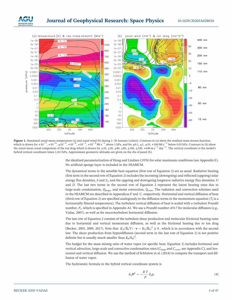
Figure 1. Simulated zonal‐mean temperature (a) and zonal wind (b) during 1–30 January (colors). Contours in (a) show the residual mass stream function,

which is drawn for +10−7

, +10−6

, ±10−5

, +10−4

, +10−3

, +10−2

Mt s−1

above 1 hPa, and for ±0.1, ±1, ±10, +100Mt s−1

below 0.03 hPa. Contours in (b) show

the zonal‐mean zonal component of the ion drag which is drawn for ±10, ±20, ±40, ±80, ±160, ±320, +640m s−1

day−1

. The vertical coordinate is the model's

hybrid vertical coordinate times 1,013 hPa. Approximate geometric altitudes are given on the rhs of panel (b).



whereΦh ¼ g ~z, g ¼ 9:81m s−2, and ~z is the geopotential height. For postprocessing of model data, the geo-

potential height is converted into the geometric height, z, using z ¼ ~z ðae þ ~zÞ=ae, where ae is the Earth

radius. The model equations are completed by the continuity equation:

∂t∂ηpþ ∇ · ð ∂ηp v Þþ∂η ð ∂ηp _η Þ ¼ 0 ; (5)

the evolution equation for the surface pressure and expressions for the vertical velocities,

∂tps ¼ −

Z

1

0

∇ · ð∂ηp vÞ dη (6)

_η ¼ −

1

∂η pb ∂t ps þ

Z

η

0

∇ · ð ∂~ηp v Þ d~η

0

@

1

A (7)

_p ¼ b ð v · ∇Þ ps −Z

η

0

∇ · ð ∂~η p v Þ d~η ; (8)

by flux boundary conditions for the vertical diffusion terms in Equations 1–3:

−

p

R TðKz þ νzÞ

g p ∂ηv

R T ∂ηp

� �

surf

¼ p

R T

h i

LCD vL (9)

−

p

R T

Kz

Pr

þ νz0:7

� �

g p ∂ηT

R T ∂ηp−

Kz

Pr

g

cp

� ��

surf

¼ p

R T

h i

LCD ð TL − Ts Þ ¼ f sens (10)

−

p

R TðKz þ νzÞ

g p ∂ηq

R T ∂ηp

� �

surf

¼ p

R T

h i

LCDq ð qL − qs Þ ¼ f latent ; (11)

and by the surface energy budget,

csurf ∂tTs ¼ S − Sr þ D − U½ �η¼1 þ cp f sens þ ℓ f latent þ hocean: (12)

In Equations 9–11, the index “L” denotes the upper edge of the Prandtl layer, which is identified with the

lowest full model layer. The latent heat per unit mass is ℓ ¼ 2:5 × 106 J/kg. The specific humidity at the

surface, qs, is defined in Equation C4 (see Appendix C). Furthermore, csurf (λ, ϕ) and hocean(λ, ϕ) are the

prescribed heat capacity of the surface and the lateral oceanic heat flux convergence, respectively (see also

Becker & Vadas, 2018, their Figure 1). Details of the exchange coefficient at the surface are given in

Appendix A. The flux boundary conditions (9)–(11) are completed by corresponding conditions at the

model top where the fluxes are set to 0. Likewise, the vertical velocity (7) is subject to kinematic boundary

conditions at the surface and at the model top (Simmons & Burridge, 1981).

Because of the change of atmospheric composition with increasing altitude, the gas constant, R, and the heat

capacity at constant pressure, cp, are no longer constant in the thermosphere. We account for the variations

of R and cp by assuming a monotonic dependence of the gas constant on the pressure. In this case, the heat

capacity at constant pressure becomes a function of the temperature alone. This constraint is derived in

Appendix D. Since the HIAMCM employs sensible heat as prognostic thermodynamic variable and pressure

as a vertical coordinate above the tropopause, the functions R(p) and cp(T) as given in Appendix D allow for a

straightforward extension of the dynamical core into the thermosphere.

Semi‐implicit time stepping is performed with regard to the actual global‐mean temperature, and it incorpo-

rates linear contributions from the nonhydrostatic correction, as well as from horizontal and vertical diffu-

sion of momentum, sensible heat, and water vapor using globally averaged diffusion coefficients (see

Appendix A and Figure A1).

In the following we show first HIAMCM results for the northern hemispheric winter. We extracted an initial

condition for 1 December from the free‐running T240L220 KMCM used in Vadas and Becker (2019). We

then added 40 model layers and used the spectral expansion coefficients of the uppermost layer from the



T240L220 KMCM to populate the additional layers. The HIAMCM T240L260 was then integrated for

another nine model weeks. The same procedure was applied to the southern winter, using an initial condi-

tion from the former KMCM for 1 July. In each case, equilibrated dynamical states were reached after a few

weeks of integration. Results presented in this paper refer to the integration periods from 1 to 30 January and

from 1 to 20 August, which are the currently available model data with equilibrated dynamics.

3. Results

3.1. Zonal‐Mean Picture

Before analyzing the simulated GWs in detail, we consider the usual zonal‐mean diagnostics. The colors in

Figure 1 show the zonal‐mean temperature and zonal wind averaged in January. The model result for the

lower and middle atmosphere is consistent with current knowledge based on either GW‐resolving GCMs

(e.g., Becker & Vadas, 2018; Watanabe &Miyahara, 2009) or comprehensive chemistry‐climate models with

parameterized GWs (e.g., Smith, 2012, Figures 1 and 2). That is, the cold summer mesopause and warm win-

ter stratopause are linked to the residual circulation (contours in panel a). The first wind reversals in the

summer MLT from westward to eastward flow (at ∼ 10−4 hPa in Figure 1a) and from eastward to westward

flow (at ∼ 5 × 10−6 hPa in Figure 1a) are too high in altitude by 1–2 scale heights each when compared to

CIRA‐86 (Fleming et al., 1990). This shortcoming is discussed below further. In contrast to models with para-

meterized GWs, a GW‐resolving model does not simulate a reversal from eastward to westward flow with

increasing height in the winter polar MLT on average, which is more consistent with observational data

(see again Smith, 2012, Figures 1 and 2).

The simulated temperature strongly increases with height between about 100 and 150–200 km to an exo-

spheric temperature of ∼ 900–1000 K. This is consistent with the global mean energy budget depicted in

Figure F1b, showing an approximate balance between extreme ultraviolet (EUV) heating from the Sun

and cooling due to downward molecular heat conduction above z ∼ 200 km. The thermospheric mean zonal

wind is westward in summer and eastward in winter. The latter is consistent with a mean temperature

decrease from the summer to the winter pole, which is expected from a radiatively determined state.

However, this temperature gradient is reduced by a summer‐pole‐to‐winter‐pole circulation at z ∼

200–450 km that is largely driven by the zonal component of the mean ion drag (contours in Figure 1b).

These thermospheric patterns are consistent with corresponding results from other global models (e.g.,

H.‐L. Liu et al., 2018; Miyoshi et al., 2014). Due to the lack of ion chemistry, geomagnetic forcing, and ener-

getic particle precipitation, the HIAMCM does not reproduce the observed westward mean winds in the

thermosphere over the northern polar cap during wintertime (Drob et al., 2015).

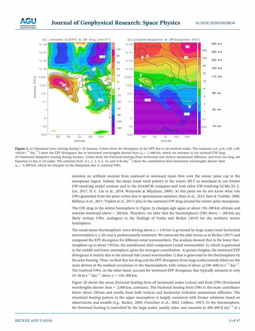
Figure 2a shows the EPF divergence from all resolved waves (colors) along with the contribution from the

resolved GWs (contours). This GW drag is identified as the EPF divergence due to horizontal wavelengths

smaller than ∼ 2,000 km (horizontal wavenumbers larger than 20). The simulated GW drag in the middle

atmosphere compares well with other model estimates (e.g., Fomichev et al., 2002; Smith, 2012).

However, the eastward GW drag around the summer polar mesopause and the summer mesopause itself

is too high in altitude by about 10 km. This is related to the wind reversal being too high in altitude as well,

as mentioned above. The likely reasons for this shortcoming are (1) that the present model tuning is not suf-

ficient, for example, regarding the turbulent diffusion scheme that induces GW dissipation, and (2) that the

model resolution is still too coarse to resolve the GWs necessary for a more realistic eastward GW drag in the

summer MLT. On the other hand, the model produces realistic dynamics of the winter middle atmosphere,

including the westward GW drag due orographic and nonorographic GWs from the upper stratosphere to

the upper mesosphere poleward of about 30°N (Figure 2a). Furthermore, there is a significant eastward

GW drag in the winter mesopause region and lower thermosphere. This feature was found previously for

the southern winter middle atmosphere and was shown to be due to secondary GWs (Becker & Vadas, 2018).

In that work, the secondary GWs were generated by imbalances from the intermittent body forces (i.e.,

horizontal accelerations) resulting from the primary GWs that dissipate in the winter stratopause region.

The mean wind then favored the upward propagation of eastward secondary GWs, which dissipate in the

mesopause region and in the lower thermosphere. The current model simulation confirms that such an east-

wardGWdrag is also found in the northernwinter hemisphere. As discussed in Becker andVadas (2018), this

eastward GW drag from secondary GWs is the main reason why GCMs with resolved GWs usually do not



simulate an artificial reversal from eastward to westward mean flow over the winter polar cap in the

mesopause region. Indeed, the mean zonal wind pattern in the winter MLT as simulated in our former

GW‐resolving model versions and in the HIAMCM compares well with other GW‐resolving GCMs (H.‐L.

Liu, 2017; H.‐L. Liu et al., 2014; Watanabe & Miyahara, 2009). At this point we do not know what role

GWs generated from the polar vortex due to spontaneous emission (Sato et al., 2012; Sato & Yoshiki, 2008;

Shibuya et al., 2017; Triplett et al., 2017) play in the eastward GW drag around the winter polar mesopause.

The GW drag in the winter hemisphere in Figure 2a changes sign again at about 150–200 km altitude and

remains westward above ∼ 200 km. Therefore, we infer that the thermospheric GWs above ∼ 200 km are

likely tertiary GWs, analogous to the findings of Vadas and Becker (2019) for the southern winter

hemisphere.

The zonal‐mean thermospheric wave driving above z ∼ 150 km is governed by large scales (total horizontal

wavenumbers n≤ 20) and is predominantly westward. We extracted the tidal waves as in Becker (2017) and

computed the EPF divergence for different zonal wavenumbers. The analysis showed that in the lower ther-

mosphere up to about 150 km, the semidiurnal tidal component (zonal wavenumber 2), which is generated

in the middle and lower atmosphere, gives the strongest contribution. At greater heights, the westward EPF

divergence is mainly due to the diurnal tide (zonal wavenumber 1) that is generated in the thermosphere by

the solar heating. Thus, we find that ion drag and the EPF divergence from large scales (mainly tides) are the

main drivers of the residual circulation in the thermosphere, with values of about ±(100–600) m s−1 day−1.

The resolved GWs, on the other hand, account for westward EPF divergence that typically amounts to only

10–20 m s−1 day−1 above z ∼ 150–200 km.

Figure 2b shows the mean frictional heating from all horizontal scales (colors) and from GWs (horizontal

wavelengths shorter than ∼ 2,000 km, contours). The frictional heating from GWs is the main contributor

below about 100 km and results from both vertical and horizontal turbulent momentum diffusion. The

simulated heating pattern in the upper mesosphere is largely consistent with former estimates based on

observations and models (e.g., Becker, 2009; Fomichev et al., 2002; Lübken, 1997). In the thermosphere,

the frictional heating is controlled by the large scales, mainly tides, and amounts to 200–400 K day−1 at z

Figure 2. (a) Simulated wave driving during 1–30 January. Colors show the divergence of the EPF due to all resolved scales. The contours (±5, ±10, ±20, ±40,

+80m s−1

day−1

) show the EPF divergence due to horizontal wavelengths shorter than λh ∼ 2, 000 km, which we interpret as the resolved GW drag.

(b) Simulated dissipative heating during January. Colors show the frictional heating (from horizontal and vertical momentum diffusion, and from ion drag, see

Equation 2) due to all scales. The contours (0.01, 0.1, 1, 2, 4, 8, 16, and 32 K day−1

) show the contribution from horizontal wavelengths shorter than

λh ∼ 2, 000 km, which we interpret as the dissipation due to resolved GWs.



∼ 200–400 km. This is consistent with the fact that also the EPF divergence in the thermosphere is mainly

due to large scales. Combining Figure 2b with the global‐mean results given in Figure A3 suggests that

the damping of the tides in the thermosphere is mainly due to ion drag and to a lesser extent due to

molecular viscosity. Since the averaged frictional heating in the thermosphere is mainly due to the tides,

the generation and dissipation of the diurnal tide is the major, Lorenz‐type energy cycle above about 150 km.

Further inspection of themodel results shows that the GWs are mainly dissipated bymomentum diffusion at

all heights and that dissipation by ion drag is unimportant for the GWs. The reason is that diffusion is highly

scale selective such that GWs, which have much smaller scales than the tides, are more efficiently damped

by diffusion rather than by ion drag. In other words, the damping rates resulting from viscosity are much

larger than those resulting from ion drag for most thermospheric GWs. This holds particularly for GWs hav-

ing intrinsic periods less than ∼ 2 hr, even during daytime solar maximum conditions (see section 3.2. in

Vadas, 2007 and pages 241 and 242 in Gossard & Hooke, 1975).

Our simulated zonal‐mean effects from the GWs in the thermosphere (e.g., westward zonal GW drag of

about 10–20 m s−1 day−1 and energy deposition of about 10–30 K day−1) are at least 1 order of magnitude

smaller compared to the previous model results of Yigit et al. (2009). In that study, a conventional GW para-

meterization with lower stratospheric launch level parameters was extended into the thermosphere and

showed very strong GW‐mean flow interactions in the thermosphere. Miyoshi et al. (2014) used a

GW‐resolving GCM and also found strong zonal‐mean GW drag of up to +200m s−1 day−1 above 200 km.

This drag is comparable in magnitude with the westward EPF divergence in Figure 2 from all waves (colors).

However, this result of (Miyoshi et al., 2014, their Figure 3) does not contradict our result because those

authors used zonal and meridional wavenumbers larger than 5 to define the GW drag, which includes hor-

izontal wavelengths up to 8,000 km, whereas our definition of GWs includes only total horizontal wavenum-

bers larger than 20 (horizontal wavelengths shorter than 2,000 km). Thus, large‐scale inertia GWs and tidal

components are included in the specific definition of the GW drag used in Miyoshi et al. (2014).

Furthermore, the expression for the complete EPF divergence (e.g., Equations (15) and (16) in

Becker, 2017) must be used to estimate the wave‐mean flow interaction, because tides and inertia GWs have

large Stokes drifts, which yield an EPF divergence that can be opposite to the vertical momentum flux con-

vergence. However, Miyoshi et al. (2014) calculated only the vertical momentum flux convergence. Other

differences between the HIAMCM and the model of Miyoshi et al. (2014) are that the HIAMCM has signifi-

cantly higher spatial resolution, as well as a physically consistent treatment of horizontal diffusion (as

opposed to utilization of hyperdiffusion).

3.2. Resolved GW Dynamics

Even though the zonal‐mean picture is very useful in the middle atmosphere, its relevance is questionable in

the thermosphere. The reason is that the instantaneous wind variations due to the tides and GWs are larger

than or at least comparable to the mean winds there. In the following we analyze the simulated instanta-

neous GW variations in the thermosphere in relation to the tides and to the GW sources at lower altitudes.

Figure 3 shows snapshots of GW‐related relative density fluctuations from the lower stratosphere to the

upper thermosphere in theNorthernHemisphere on 4 January. Here, we used the total horizontal wavenum-

bers larger than 30 (n> 30, horizontal wavelength shorter than ∼ 1,350 km) to define the GW perturbations.

In panel (a), the deformed polar vortex in the lower stratosphere at z ¼ 15 km is indicated by the white con-

tours representing the horizontal stream function. This panel features several GW packets. For example,

there are GW packets over Alaska (and Northwest Canada) and over the Rocky Mountains (and farther

downstream). These are presumably orographically generated, because the GW phases at 15 km are roughly

perpendicular to the directions of the large‐scale wind (southeastward over Alaska and eastward over the

Rocky Mountains), and these directions are roughly the same in the lower troposphere for these two cases

(not shown). This interpretation is also consistent with the fact that the GW packet over and downstream

of the RockyMountains is no longer visible atz ¼ 60km (panel b)where the large‐scalewind has turned from

eastward to southward, as can be inferred from comparing the horizontal stream functions in panels (a) and

(b). Hence, the orographic GWs must have encountered a critical level. The GW packet at z ¼ 15 km over

Alaska is also no longer visible at z ¼ 60 km. This is presumably because in this region the background wind

has become very weak (as is indicated by the larger distances between stream function contours compared to

panel a), thereby inducing wave breaking and subsequent damping by turbulent diffusion for these



orographic GWs.Note that in theHIAMCM, both the vertical and horizontal diffusion coefficients depend on

the local and instantaneous Richardson number (see Equations A6–A11) such that the smallest‐scale GWs

that become dynamically unstable are strongly damped. This parameterizes the energy cascade at

unresolved (subgrid) scales. For GWs having horizonal wavelengths larger than λh ∼ 400 km, part of this

cascade is resolved in the HIAMCM (Becker & Vadas, 2018).

In addition to the orographic GWs discussed above, Figures 3a and 3b feature inertia GWs that are likely

associated with spontaneous emission. The GWs generated by that mechanism often show localized GW

packets in the exit region of a jet with the GW phases approximately perpendicular to the streamlines

(e.g., O'Sullivan & Dunkerton, 1995; Zhang, 2004), for example, at 15 km over the East Atlantic from

North Africa to Brittany and at 15 km over the Pacific at about 170°E. Or they show spirals closely aligned

with (approximately parallel to) the streamlines of the vortical flow (e.g., Sato & Yoshiki, 2008). This occurs,

for example, in Figure 3a at ∼ 30°N from the Pacific to the Atlantic Ocean over North America and in

Figure 3b from the Eastern Mediterranean to Siberia.

From the lower thermosphere on, tidal variations have strong amplitudes while kinematic viscosity (mole-

cular viscosity divided by density) increases rapidly with altitude. As a result, only GWs having large intrin-

sic phase speeds (of at least ∼ 150m s−1) can propagate to high altitudes in the thermosphere (Vadas, 2007).

Model results show that wintertime primary and secondary GWs dissipate from dynamical instability in the

Figure 3. North polar projection (poleward of 20°N) of relative density perturbations (colors) from GWs with horizontal wavelengths shorter than λh ∼1,350 km (total wavenumbers n > 30) at 15, 60, 140, and 300 km on 4 January: (a–c) 0 UT and (d) 6 UT. Here, the model data have been interpolated from the

model surfaces to these geometric heights. The polar vortex at 15, 60, and 140 km is indicated by the horizontal stream function with white contours, whereby

the minima and maxima are marked by gray capital letters L and H, respectively. In the Northern Hemisphere, the flow is clockwise (counterclockwise)

around the maxima (minima) of the stream function.



upper MLT (Becker & Vadas, 2018; Vadas & Becker, 2019). The resulting body forces lead to the generation

of secondary and tertiary GWs that are visible as concentric rings of the GWs in horizontal snapshots above

and below the body force (Vadas et al., 2003, 2018). Such an example is visible in Figure 3c (at z ¼ 140 km)

with the center of the concentric rings at about 90°W and 50°N (over the Rocky Mountains). At this altitude,

the largest amplitudes are seen for the GWs propagating northwestward, westward, and southwestward

away from this center. As indicated by the stream function contours in Figure 3c, the northwestward propa-

gation direction is favored by the southeastward large‐scale flow over Alaska and western Canada.

This picture is strongly variable in time due to the tidal motions. Moreover, the tidal winds have strong con-

tributions from both the stream function and the velocity potential. Therefore, the stream function is no

longer a valid representation of the background flow above z ∼ 150 km. Figure 3d shows a snapshot at

z ¼ 350km and 6 hr later than Figures 3a–3c in order to allow the GWs resulting frommultistep vertical cou-

pling to reach the upper thermosphere. Large‐scale winds associated with the diurnal migrating tide (not

shown) are strongly southward (northward) over North America (Siberia) at this time since it is LTmidnight

(noon) there (Roble & Ridley, 1994). The GWs resolved in the HIAMCM propagate approximately against

this tidal wind, which is consistent with the observational findings of Crowley and Rodrigues (2012).

Figure 4 shows vertical snapshots that illustrate the GW propagation directions of some of the strong GW

events seen in Figure 3 (using the same definition for GW perturbations). The longitude‐height cross section

in Figure 4a at 46°N focuses on the aforementioned lower stratospheric orographic GW event over the Rocky

Mountains. The inclination of the GWphases in the stratosphere shows that the GWpacket at 120–90°W and

z≤ 50 km propagates westward with respect to the wind, thereby confirming that it is generated by eastward

wind flow over the Rocky Mountains. The GW phases become flat above z ∼ 50 km because the large‐scale

zonal wind turns westward in this regime (the black contour in Figure 4a marksu ¼ 0). This induces the dis-

sipation of orographic GWs beneath their critical level. According to Vadas et al. (2003) and Vadas

et al. (2018), the resulting body force creates an imbalance in the background flow and thereby results in

the generation of secondary GWs. These secondary GWs propagate upward and downward in all horizontal

directions except perpendicular to the direction of the body force (i.e., they do not propagate northward or

southward in this particular example). The amplitudes of the upward propagating secondary GWs are small

at their generation altitude (e.g., z ∼ 50 km here) but become large in the mesopause region. In the example

depicted in Figure 4a, the secondary GWs are seen at z ∼ 60–80 km and from about 120°W to 80°W. The

increasing eastward wind from z ∼ 60 to 100 km induces dissipation of the eastward propagating secondary

GWs. The westward wind shear above z ∼ 100 km in the longitude sector from 110°W to 80°W then induces

the dissipation of the westward secondary GWs. As shown in Vadas and Becker (2019), the body forces that

result from the dissipation of secondary GWs in turn lead to the generation of tertiary GWs. The tertiary GWs

induced by the mountain wave event over the Rocky Mountains can be seen at altitudes above z ∼ 120 km at

130–60°W in Figure 4a; these same GWs appear as concentric rings at z ¼ 140 km in Figure 3c. Figure 4a

furthermore indicates that some of the GWs in the broad tertiary GW spectrum dissipate by 140 km.

A closer inspection of the model data showed that the orographic event visible in Figure 4a over the Rocky

Mountains started on 3 January at ∼ 3 UT and that the secondary GWs first appeared in the upper meso-

sphere about 6 hr later (on 3 January at ∼ 9 UT). Hence, in this particular example, the secondary GWs take

about 6 hr to propagate from the upper stratosphere to the upper mesosphere, corresponding to a vertical

group velocity of ∼ 5 km/hr.

Figure 4b shows a latitude‐height cross section at 65°E to further illustrate the aforementioned GW genera-

tion in the stratopause region by spontaneous emission. From Figure 3b, vortex‐generated GWs propagate

southward at z ∼ 60 km, ∼ 65°E, and ∼ 35°N. (According to Sato and Yoshiki (2008), GWs generated from

the polar night jet propagate equatorward on the equatorward side of the jet.) Therefore, the inclination

of the GW phases in Figure 4b implies downward propagation at z ∼ 30–60 km at 30–40°N. Furthermore,

the meridional wind contours show a southward vertical shear at z ∼ 65–80 km such that the upward and

southward propagating GWs in this example dissipate by z ∼ 70–80 km. The GW activity in the lower ther-

mosphere in Figure 4b results from the lateral propagation of GWs generated by other sources but may also

include secondary GWs created by body forces from the dissipation of the vortex generated GWs.

The latitude‐height and longitude‐height snapshots in Figures 4c–4f illustrate the meridional (c and d) and

zonal (e and f) propagation of GWs from Figure 3d at approximately midnight, noon, 6 LT, and 18 LT,



respectively. The large‐scale thermospheric wind (not shown) is primarily due to the diurnal tide and is

approximately southward at midnight (c), northward at noon (d), westward at 6 LT (e), and eastward at

18 LT (f) in the Northern Hemisphere. The GWs at z ≥ 180 km have very long vertical wavelengths, in

agreement with linear viscous theory (Fritts & Vadas, 2008; Vadas, 2007). Importantly, the thermospheric

GWs propagate approximately against the background wind, that is, northward, southward, eastward, and

Figure 4. Horizontal‐vertical cross sections of the GW density perturbations focusing on the GW events seen in Figure 3 on 4 January. Contours in

panel a (panel b) show the large‐scale zonal wind (meridional wind) for −50, 0, and +50m s−1

using dashed white, solid black, and solid white contours,

respectively. The white arrows in (c) and (d) mark fishbone structures. See text for more details.



Figure 5. (a–d) North polar projection (poleward of 20°N) of 6‐hourly consecutive snapshots of relative density perturbations (colors) owing to GWs having λh< 1,350 km at z ¼ 300 km on 2–3 January. White arrows show the instantaneous large‐scale horizontal wind field. A 100m s

−1black arrow is shown between

panels (c) and (d) as a scale. (e and f) Same as Figures 3a and 3b but on 2 January 1 UT and with larger color and contour intervals. The latitudes 40°N and

60°N are indicated by black circles.



westward in Figures 4c–4f, respectively, as seen by the inclination of the GW phases. In general,

Figures 4c–4f indicate that larger GW scales dominate at z≥ 150 km compared to lower altitudes. This could

be because tertiary GWs are generated at z ∼ 120–160 km (see the fishbone structures at these altitudes, two

of which are marked by white arrows in panels c and d) or because those GWs generated at lower altitudes

having large horizontal wavelengths and phase speeds become dominant at z > 150 km.

The propagation of GWs in the thermosphere is further illustrated in Figures 5a–5d where we show 6‐hourly

snapshots of GW perturbations and the large‐scale horizontal wind at z ¼ 300 km on 2–3 January. We see a

24‐hourly clockwise rotation of the predominant GW propagation directions that is linked to the clockwise

rotation of the diurnal tide in the Northern Hemisphere. This HIAMCM result is typical for the Northern

Hemisphere winter (not shown). Figures 5a–5d also show that the GW propagation is not precisely opposite

to the tidal wind but lags somewhat (Crowley & Rodrigues, 2012).

Figures 5e and 5f illustrate the GWs and the polar vortex in the upper troposphere and around the strato-

pause at 2 January, 1 UT. At this time, the polar vortex was strong and therefore favored the vertical propa-

gation of primary GWs into the stratopause region. In particular, a strong GW event is seen over

Siberia/Mongolia at middle to high latitudes (panels e and f), which presumably gives rise to tertiary GWs

in the thermosphere. These GWs are likely seen as concentric rings in Figure 5c, the center of which is

located downstream over northeastern China. Additionally, large‐amplitude GWs are also excited in the

jet‐exit region at z ¼ 15 km over the Rocky Mountains (panel e) and are also seen in the stratopause region

(panel f). There are some weak ring‐like structures in Figure 5a at z ¼ 300 km centered over the Rocky

Mountains, which may indicate secondary or tertiary GWs induced by this event.

Given our arguments for the multistep vertical coupling mechanism to explain the medium‐ and large‐scale

GWs in the winter thermosphere at middle and high latitudes (Vadas & Becker, 2019), the occurrence rate

and strength of these tertiary GWs should correlate with the strength of the polar vortex. Frissell et al. (2016)

used a system of high‐frequency radars in the North American sector to observe daytimemedium‐scale TIDs

(MSTIDs) from 2012 to 2015. Such MSTIDs are presumably caused by GWs via neutral‐ion collisions (e.g.,

Hocke & Schlegel, 1996; Nicolls et al., 2014; Vadas & Nicolls, 2009). Indeed, Frissell et al. (2016) found that

the occurrence of the MSTIDs is strongest between the onset and the breakdown of the polar vortex and that

wintertime MSTID activity is minimum when the polar vortex is weak.

A prerequisite for the HIAMCM to yield reliable results for the GWs in the thermosphere is that the observed

tidal variations are reproduced. We tuned the solar heating in the thermosphere (see Appendix F) such that

the tidal wind variations from the climatological wind model HWM14 (Drob et al., 2015) and the climatolo-

gical temperature model MSIS (Hedin, 1991) are simulated reasonably well in the upper thermosphere.

Figure 6 shows data from HWM14 and MSIS for 12UT on 5 January 2014, corresponding to solar maximum

conditions with weak particle precipitation, and the corresponding HIAMCM data in early January at 59°N.

While the overall structure and phases of the observation‐based tidal variations are captured by

the HIAMCM, there are some discrepancies, especially in the lower tomiddle thermosphere where little data

was incorporated into HWM14 and MSIS. The differences in the middle to upper thermosphere are likely

because HWM14 and MSIS are climatological models and HIAMCM incorporates variability from below.

We now determine the typical scales of the GWs simulated in the thermosphere by the HIAMCM. As an

example we pick the equatorward propagating GWs over the North Atlantic on 2 January at 18 UT in

Figure 5c. Such GWs would represent the aforementioned daytime MSTIDs observed by Frissell et al. (2016)

over the North American sector. Figure 7 shows latitude‐height (a and c) and latitude‐time (b and d) cross

sections at 45°W on 2 January. The upper panels show the propagation of GWs having horizontal wave-

lengths λh ¼ 400–2,000 km (horizontal wavenumbers 20–100), while the lower panels refer to λh ¼ 165–

400 km (horizontal wavenumbers 100–240). The inclination of the GW phases in panels (a) and (c) indicates

very long vertical wavelengths and southward propagation in the thermosphere, as expected. The GWs hav-

ingλh ¼ 400–2,000 km give the predominant contribution to the relative density fluctuations (see color scale

at the rhs of each panel). In general, we find ground‐based periods of 1 hr ≤ τ ≤ 2 hr, for horizontal wave-

lengths of 400 km ≤ λh ≤ 2,000 km, and 20min ≤ τ ≤ 40min, for 165 km ≤ λh ≤ 400 km.

In the keograms of Figures 7b and 7d, some of the GW phases are marked by black solid lines, and the cor-

responding GW packets are enumerated from 1 to 4. Assuming southward propagation, we obtain



horizontal wavelengths of ∼ 350–1,100 km and ground‐based periods of ∼ 25–90 min. These correspond to

ground‐based phase speeds of ∼ 205 m s−1 for Packet 1, ∼ 245m s−1 for Packet 2, and ∼ 195 m s−1 for

Packets 3 and 4. These large phase speeds are comparable to the values given by Frissell et al. (2016) for

MSTIDs. Furthermore, since these GWs propagate against the tidal background wind of ∼ 50–100m s−1,

their intrinsic phases speeds are ∼250–350m s−1.

Are the GWs from Figure 7 compatible with the former concept that the predominant GWs in the thermo-

sphere at middle and high latitudes are primary GWs generated in the troposphere (e.g., Yigit &

Medvedev, 2017)? To answer this question, we consider the dispersion relation for nonviscous GWs having

medium or high frequencies:

Figure 6. Comparison of tidal winds from the (a and c) HWM14 (Drob et al., 2015) and temperatures from the (e) MSIS (Hedin, 1991) with the (b, d, and f)

HIAMCM simulation (large‐scale flow including horizontal wavenumbers n< 30 only) for early January at 59°N.



ω2I ¼

N2 k2h

k2h þm2 þ 1=ð4H2Þ

: (13)

Here, ωI is the intrinsic frequency, N is the buoyancy frequency for constant background temperature, kh is

horizontal wavenumber vector, m is the vertical wavenumber, and H is the density scale height. According

to Vadas et al. (2019), a conservative estimate for the maximum possible value of the rhs of Equation 13 is

obtained when both the horizontal and vertical wavelengths are large against 4πH, yielding ω2I < 4H2N2

k2h. The reasoning is that k

2h≪1=ð4H2Þ for large enough λh and that λz becomes very large when a vertically

propagating GW is close to reflecting. Using N2 ¼ g2=ðcpTÞ and c2s ¼ cp ðcp − RÞ−1R T for the sound speed

squared, we obtain the following constraint for the maximum intrinsic horizontal phase speed of a GW:

c2I ph < 4ðcp − RÞR

c2pc2s ¼ rc csð Þ2 ; rc ¼ 2

ffiffiffiffiffiffiffiffiffiffiffiffiffiffiffiffiffiffiffiffi

ðcp − RÞRp

cp: (14)

The black solid curve in Figure 8a shows the speed of sound from theHIAMCMduring January and averaged

from 50°N to 75°N. The dashed curve shows the maximum intrinsic phase speed according to Equation 14,

where the factor rc is given by the dashed curve in Figure 8b (including R ¼ RðpÞ and cp= cp(T) from

Appendix D). The blue curves show v þ 195 m s−1 and v þ 245 m s−1, where v is the large‐scale meridional

wind at 45°W, averaged from 50°N to 75°N and from 16:00 to 20:30 UT on 2 January (see Figure 7).

Assuming that the (southward) ground‐based horizontal phase speeds of the GWs are approximately con-

stant with altitude, these blue curves are height profiles of the inferred intrinsic phase speeds of the GWs

in Figure 7d. Because of the strong northward background winds at mesopause altitudes, the fastest GWs

Figure 7. Southward propagating GWs in the thermosphere over the North Atlantic at 45°W around 18 UT (daytime). (a) Latitude‐height cross section at 18 UT

and (b) keogram at 250 km from 14 to 20.30 UT of the relative density fluctuations due to GWs having 400 km < λh ≤ 2,000 km. (c and d) Like (a) and (b) but

for 165 km ≤ λh ≤ 400 km. The black solid lines in panels (b) and (d) mark some GW packets that are enumerated from 1 to 4. Assuming southward

propagation, we obtain the following approximate horizontal wavelengths (λh), ground‐based periods (τ), and ground‐based phase speeds (ch ¼ λh=τ): λh ∼

1,100 km, τ ∼ 90min, and ch ∼ 205m s−1

for GW packet 1; λh ∼ 365 km, τ ∼ 25min, and ch ∼ 245m s−1

for GW packet 2; and λh ∼ 350 km, τ ∼ 30min, and ch ∼

195m s−1

for GW packets 3 and 4.



would have intrinsic horizontal phase speeds that exceed the speed of sound near the mesopause. Therefore,

these GWs are most likely generated in the thermosphere. Moreover, even the slower GWs may meet the

reflection criterion near the mesopause.

Figure 5c suggests that the concentric GWs analyzed in Figure 7 all originate from the same source over

northeastern China, which creates ring‐like structures of GWs propagating away from this source. Since

we found that the faster GWs from that source are generated in the thermosphere, it is likely that all of

the concentric GWs analyzed in Figure 7 are generated in the thermosphere. The same argument was also

applied in Vadas and Becker (2019).

The situation depicted in Figures 5 and 7 is typical for the GWs simulated by the HIAMCM in the northern

winter thermosphere at z ∼ 200–400 km. Furthermore, the wintertime GWs at z < 70 km typically have hor-

izontal phase speeds <100m s−1. Since these phase speeds are too slow for the corresponding GWs to survive

viscous damping and propagate to∼ 200–400 km, this suggests that most of the wintertime GWs at these alti-

tudes are likely generated above the mesopause.

3.3. Nonhydrostatic Effects

For the wave packets inspected in Figures 7c and 7d, the shortest intrinsic periods are less than 20min. Since

the buoyancy period is about 10–12 min in the 200–400 km region, these GWs are subject to nonhydrostatic

effects. In the following we analyze the effect of the nonhydrostatic correction introduced in section 2 and

Appendix B.

If high‐frequency GWs are described using hydrostatic dynamics, the k2h term in the denominator of the dis-

persion relation (13) is neglected. This leads to an overestimation of the intrinsic frequency and, hence, of

the ground‐based frequency and phase speed. Furthermore, the sensible heat equation in the anelastic

approximation yields (see Becker, 2017, Appendix)

T2a ¼

g2

c2p ω2I

w2a (15)

for the relation between the GW amplitudes of temperature (Ta) and vertical wind (wa) in the conservative

case. Assuming that a GW temperature amplitude is determined by energy conservation, hydrostatic

dynamics will also overestimate the vertical wind amplitudes of high‐frequency GWs. Hence, the

HIAMCM with the nonhydrostatic correction should yield somewhat smaller horizontal phase speeds and

smaller vertical wind amplitudes for GWs in the thermosphere as compared to the hydrostatic model version.

Figure 8. (a) Upper limit for intrinsic horizontal phases speeds of GWs. Solid black: speed of sound derived from the control simulation during January,

averaged zonally and from 50°N to 75°N. Dashed black: maximum intrinsic phase speed according to Equation 14. Blue solid: v þ 195m s−1

and v þ 245m s−1

,

where v is the meridional wind at 45°W due to horizontal wavenmumbers n≤ 20 at 45°W, averaged from 50°N to 75°N and from 16:00 to 20:30 UT on

2 January. (b) The factor rc that converts the speed of sound into the maximum intrinsic phase speed (see Equation 14).



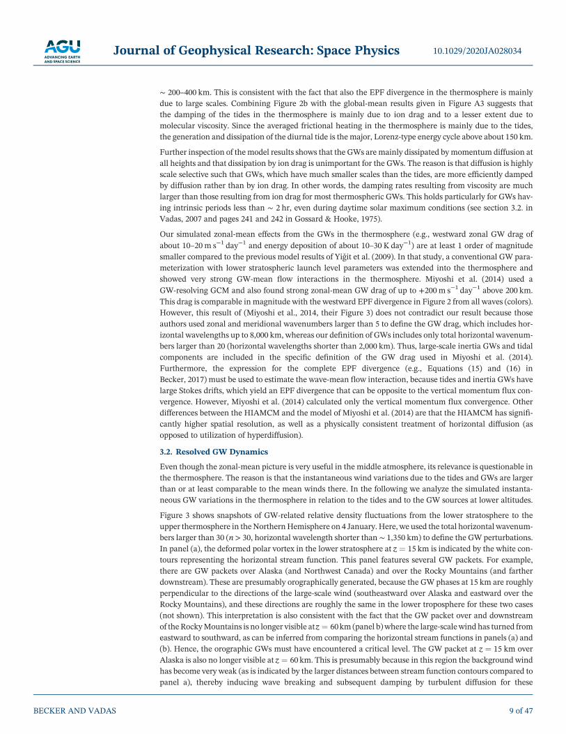
We performed a sensitivity experiment to test these expectations. For this purpose we used 6 UT on 2 January

as an initial condition to simulate the model for 3 hr without the nonhydrostatic correction. The correspond-

ing time series is then compared to that of the control simulation (i.e., with the nonhydrostatic correction

included). As an example we examine the westward propagating GWs visible in Figure 5a over the eastern

North Pacific. Figures 9a–9c illustrate this westward propagation in terms of the vertical wind at z ¼ 320

km at 6, 7:30, and 9 UT. The large‐scale GW packet visible between 40°N and 55°N east of 170°W at 6 UT

(panel a) has traveled about 15° to the west by 7:30 UT (panel b), corresponding to a phase speed of about

200m s−1. The predominant ground‐based period of this packet is about 90min. Taking into account that

the background zonal wind is about +100 m s−1 (not shown, cf. to Figure 6), the predominant intrinsic period

of this GWpacket is about 1 hr, which is still in the hydrostatic regime. Accordingly, the comparison between

the nonhydrostatic and the hydrostatic result at 9 UT in Figures 9c and 9d, respectively, does not indicate any

Figure 9. Vertical wind at z ¼ 320km over the eastern North Pacific at (a) 6, (b) 7:30, and (c) 9 UT on 2 January of the control simulation. (d) Same as (c) but for the

hydrostatic model integration. (e) Keogram of the vertical wind at z ¼ 320 km and 65°N from 6 to 9 UT. (f) Same as (e) but for the hydrostatic model integration.



notable differences for these large‐scale GWs at 40–55°N. This is, however, different for the medium‐scale

GWs over Alaska and the Bering Sea at 55–65°N and ∼ 170°W. Here, the GWs from the hydrostatic

simulation have propagated somewhat farther to the west compared to the nonhydrostatic case.

To further illustrate this difference, we show keograms of the vertical wind at z ¼ 320 km and 65°N in

Figures 9e and 9f. Assuming westward propagation, the typical ground‐based phase speed of these

medium‐scale GWs is ∼ 230m s−1 and the corresponding intrinsic phase speed is ∼ 330 m s−1. Since both

simulations start with the same initial condition, differences become visible only after about 1 hr. At 9 UT,

the GW phases have propagated farther to the west by several degrees when comparing the hydrostatic to

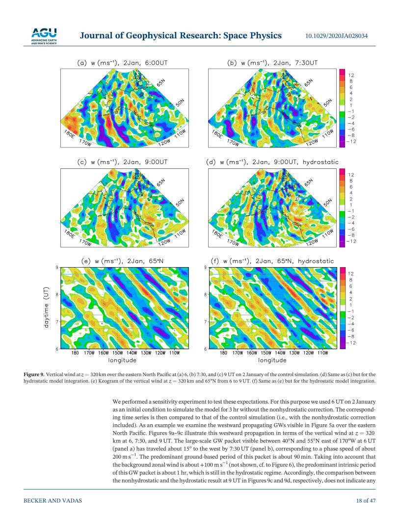
the nonhydrostatic case. These differences can be better quantified from Figure 10a, which shows the verti-

cal wind at z ¼ 320 km, 65°N, and 9 UT from both simulations. The average phase difference is about 3° in

longitude (corresponding to∼ 170 km) for the GWpacket at 140–190°W. Furthermore, the hydrostatic simu-

lation clearly shows ∼ 50% larger vertical wind variations. These differences confirm that the hydrostatic

case overestimates the GW phase speeds and vertical wind amplitudes.

The reason for these differences is further illustrated in Figure 10b, which shows different contributions to

the geopotential at 5 × 10−8 hPa, 65°N, 9 UT. The blue curve in Figure 10b shows the large‐scale geometric

height (in km) that is due to total horizontal wavenumbers n≤ 20 (corresponding to λh≥ 2,000 km). This

contribution is essentially identical in the two simulations; that is, after 3 hr of simulation from the same

initial condition, the large scales in the two model integrations do not differ notably. The gray curve in

Figure 10b is the hydrostatic part of the geopotential (Φh) in the control simulation that is due to horizonal

wavenumbers n> 20 (λh < 2,000 km). Since the nonhydrostatic geopotential, Φnh (see Equation B4) consists

mainly of small scales, we add Φnh to the gray curve, giving rise to the black curve. The differences between

the gray and black curves indicate that the nonhydrostatic correction smoothes the effective geopotential

that forces the horizontal momentum (see Equation 1). This role of the nonhydrostatic correction is particu-

larly evident from the red curve in Figure 10b, which shows the geopotential for n> 20 from the hydrostatic

simulation. Compared to both the gray and the black curves, the red curve shows much more power at small

scales, and its extrema are shifted to the west, reflecting again the unrealistically faster GW phase speed in

the hydrostatic case.

3.4. GW Hot Spots in the Winter Thermosphere

The Southern Andes/Antarctic Peninsula region is a major hot spot for wintertime orographic GWs (e.g.,

Alexander & Teitelbaum, 2011; Eckermann & Preusse, 1999; Jiang et al., 2002; Wu & Waters, 1996). These

waves are generatedwith large amplitudeswhen the predominantly eastwardwinds in the lower troposphere

are strong. In addition, there is significant wintertime GW activity in stratosphere over the circumpolar

Southern Ocean due to tropospheric GW generation by spontaneous emission (e.g., Ern et al., 2018;

Hendricks et al., 2014). The wintertime orographic GWs usually break in the upper stratosphere and lower

Figure 10. (a) Vertical wind at z ¼ 320 km, 65°N, and 9 UT on 2 January from the control simulation (black curve) and from the hydrostatic model integration

started at 6 UT (red curve). (b) Contributions to the geopotential at 5 × 10−8

hPa, 65°N, and 9 UT on 2 January: Hydrostatic geopotential due to GWs (n> 20)

from the control run (gray) and the hydrostatic integration (red). The black curve gives the result when adding the nonhydrostatic correction from the control

run to the gray curve. The large‐scale geometric height is given by the blue curve (rhs axis).



mesosphere. Due to the strong intermittency of orographic GWs (Alexander et al., 2016), the Southern

Andes/Antarctic Peninsula GW hot spot is also a region of strong generation of secondary GWs (Becker &

Vadas, 2018; de Wit et al., 2017) and presumably also of tertiary GWs that result from the body forces due

to the dissipation of secondary GWs (Vadas & Becker, 2019; Vadas et al., 2019). It is therefore likely that

the corresponding GW hot spots observed by GOCE and CHAMP at z ∼ 250–450 km (Forbes et al., 2016;

Park et al., 2014; Trinh et al., 2018) result from tertiary GWs. Because GWs can propagate large horizontal

distances in the thermosphere (e.g., Vadas & Liu, 2013), large GWactivity far from the lower‐altitude hot spot

may result. This apparent discrepancy to the observed GW hot spots can be resolved by noting that the GW

spectrum generated by a body force is broad (Vadas et al., 2003, 2018); it includes small‐medium‐scale GWs

with high frequencies that propagate close to the zenith and GWs with smaller frequencies and larger scales

that propagate closer to the horizontal. This suggests that the small‐medium‐scale GWswould form aGWhot

spot close to the Southern Andes/Antarctic Peninsula in the upper thermosphere, while GWs having larger

scales would travel larger horizontal distances and would therefore result in enhanced GW activity farther

away. Only the small‐medium‐scale GWs having large‐enough frequencies and vertical group velocities

would be visible at z ∼ 250–450 km near the geographical location of their sources. Hence, we expect an oro-

graphic GW hot spot in the stratosphere to be “mirrored” in the upper thermosphere through the multistep

vertical coupling mechanism when we only examine the small‐ to medium‐scale GWs.

Using the spectral decomposition of the temperature in terms of spherical harmonics, we compute the tem-

perature variances due to different horizontal spectral regimes of the total horizontal wavenumber: back-

ground flow (n ¼ 0…20 or λh > 2,000 km), large‐scale GWs (n ¼ 21…50 or 2,000 km > λh ≥ 800 km),

medium‐scale GWs (n ¼ 51…120 or 800 km > λh ≥ 330 km), and small‐medium‐scale GWs (n ¼ 121…

240or 330 km > λh≥ 165 km). Maps were produced by averaging the squared temperature fluctuations over

horizontal areas of about 1,000 × 1,000 km2 and averaging in time.

Figure 11 shows the resulting temperature variance maps in the Southern Hemisphere during August at 50,

70, 90, and 110 km height. In the stratopause region (first row), the major orographic hot spots (Southern

Andes/Antarctic Peninsula, New Zealand, Tasmania) show up most clearly in the medium‐scale and

small‐medium‐scale spectral regimes. Nevertheless, significant amplitudes are generated by the Southern

Andes and Antarctic Peninsula even in the large‐scale regime. With increasing altitude in the mesosphere,

however, the temperature variance in the large‐scale regime (left column) becomes roughly zonally sym-

metric. This means that these large‐scale GWs are generated presumably by the dissipation of primary

GWs resulting from flow over orography and spontaneous emission in the upper troposphere. Therefore,

the sources of these mesospheric secondary GWs reside not only over the orographic hot spot regions but

also over the circumpolar Southern Ocean (see also Becker & Vadas, 2018; Vadas & Becker, 2018).

Moreover, these waves have small‐enough vertical group velocities so that they propagate large horizontal

distances while propagating from the lower to the upper mesosphere, resulting in a roughly zonally sym-

metric distribution (Figures 11g and 11j). Also note that this distribution of large‐scale secondary GWs

around the mesopause maximizes in the polar region. The likely reason is that propagation directions

toward the south and the east are favored because the poleward mean meridional and eastward mean zonal

winds decrease with altitude in the southern winter mesosphere. It is also likely that some GW activity seen

in the large‐scale regime above z ¼ 50 km is caused by spontaneous emission from the stratospheric polar

vortex (see Figures 3b and 4b).

The medium‐scale and small‐medium‐scale temperature variances in Figure 11 (second and third columns)

show maximum values somewhat downstream (eastward and poleward) of the Antarctic Peninsula and the

Southern Andes at 70 and 90 km, which is similar to the orographic GW events analyzed in Becker and

Vadas (2018) and Vadas and Becker (2019), indicating that these GWs are mainly secondary GWs. At

z ¼ 110km, the Southern Andes/Antarctic Peninsula GW hot spot is only visible in the small‐medium‐scale

spectral regime (Figure 11l). Using temperature data from the SABER (Sounding of the Atmosphere using

Broadband Emission Radiometry) instrument onboard the TIMED (Thermosphere Ionosphere

Mesosphere Energetics Dynamics) satellite, Trinh et al. (2018) and X. Liu et al. (2019) found that this hot spot

is visible in the stratosphere and lower mesosphere, but not near the mesopause (e.g., at z ∼ 85–90 km in

Figure 2 of Trinh et al., 2018). A possible explanation is that the hot spot is partially smoothed out around

the mesopause because of horizontal propagation of (secondary) GWs.



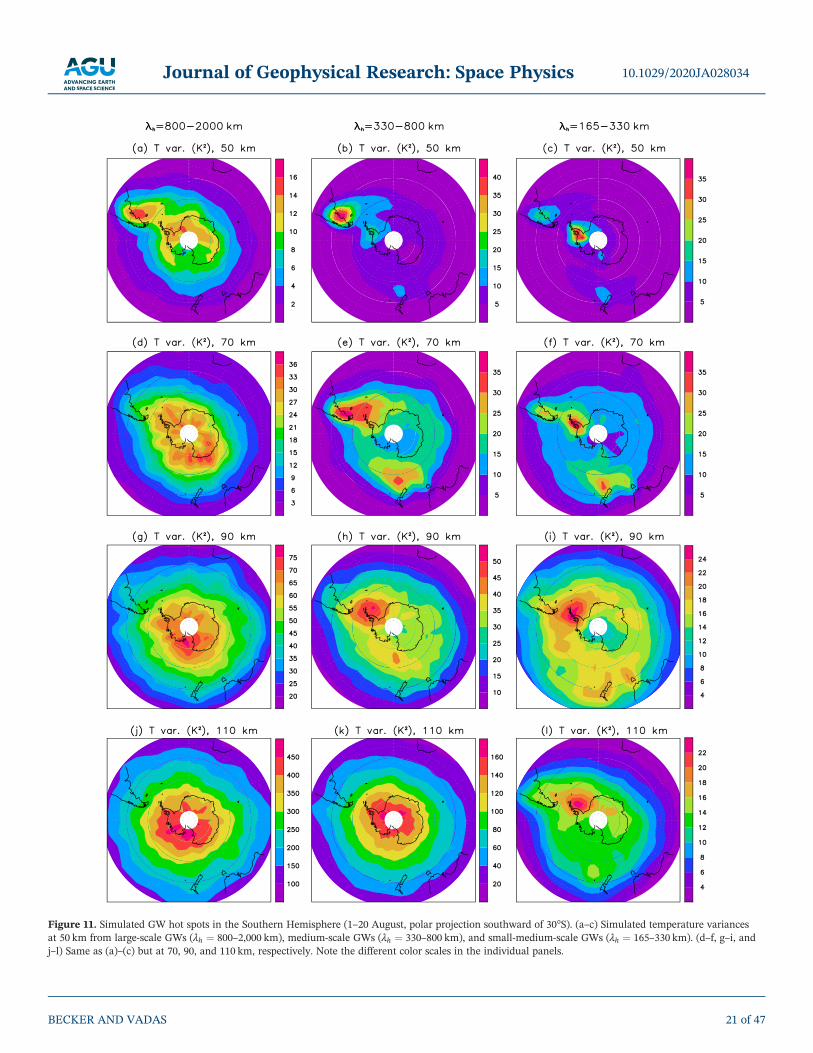
Figure 11. Simulated GW hot spots in the Southern Hemisphere (1–20 August, polar projection southward of 30°S). (a–c) Simulated temperature variances

at 50 km from large‐scale GWs (λh ¼ 800–2,000 km), medium‐scale GWs (λh ¼ 330–800 km), and small‐medium‐scale GWs (λh ¼ 165–330 km). (d–f, g–i, and

j–l) Same as (a)–(c) but at 70, 90, and 110 km, respectively. Note the different color scales in the individual panels.



Figure 12. Same as Figure 11 but at 140, 200, 300, and 380 km.



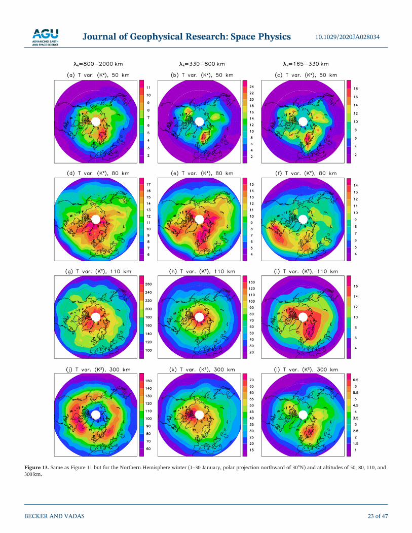
Figure 13. Same as Figure 11 but for the Northern Hemisphere winter (1–30 January, polar projection northward of 30°N) and at altitudes of 50, 80, 110, and

300 km.



The strongest and most intermittent body forces in the lower thermosphere are expected to result from the

medium‐scale and small‐medium‐scale GWs. This is because large‐scale GWs having smaller intrinsic fre-

quencies will generate weaker and less localized body forces due to their Stokes drifts and larger horizontal

scales (e.g., Fritts & Alexander, 2003; Vadas & Becker, 2018). Hence, the generation of tertiary GWs is

expected to be maximum somewhat eastward and poleward from the Southern Andes/Antarctic

Peninsula GW hot spot on average, as is seen in Figure 1 of Vadas and Becker (2019). Furthermore, tertiary

GWs having small‐medium scales and large vertical group velocities should create a GW hot spot in the

upper thermosphere.

Figure 12 shows the temperature variances analogous to Figure 11, but for the thermosphere. Indeed, theGW

hot spot near the Southern Andes/Antarctic Peninsula is visible at all altitudes for medium‐small‐scale GWs

(right column in Figure 12). This hot spot is strongest somewhat east of the Southern Andes in the thermo-

sphere, whereas the correspondingmaximum at z ¼ 90and 110 km (Figures 11i and 11l) is located east of the

Antarctic Peninsula. The large‐scale and medium‐scale temperature variances in Figure 12 (first and second

columns) are strongly indicative of GW propagation around and over the pole, creating a broad maximum at

middle to high latitudes from about 30°E to 180°E that is most pronounced at z∼ 300 km. Such an additional

broad maximum is also visible in the thermospheric results of Trinh et al. (2018, their Figures 2 and 6). The

lower two rows in Figure 12 show that the small‐medium‐scale GWs are strongly damped from 300 to 380 km

altitude, whereas the damping is much less for GWs with larger horizontal scales. This is because the com-

plete damping of GWs due to molecular viscosity, which is roughly proportional to k2h þm2

− 1=ð4H2Þ(Vadas & Liu, 2013), is included in the HIAMCM. (GCMs usually do not include molecular viscosity in the

horizontal diffusion scheme and therefore neglect k2h from molecular viscosity in the GW damping rate.)

This strong viscous damping above z∼ 300 km of small‐medium‐scale GWs having typical intrinsic horizon-

tal phase speeds of ∼ 350m s−1 (see Figure 8) is consistent with results of Vadas (2007).

Figure 13 shows the model results of the GW hot spots at different altitudes in the Northern Hemisphere

during January. Large‐scale GWs in the stratopause region (panel a) are of minor relative importance com-

pared to the Southern Hemisphere because the GW generation by spontaneous emission in the upper tropo-

sphere is weaker in the northern winter than in the southern winter due to weaker synoptic baroclinic

Rossby waves at the expense of larger planetary Rossby wave activity. The medium‐scale and small‐med-

ium‐scale GW variances at 50 km (panels b and c) reflect the orographic GW hot spots where most of the

GWs that propagate to 50 km are generated during the simulation period: Alaska, Greenland,

Scandinavia, Ural, and Mongolia/Siberia. Due to the larger number of orographic hot spots, the sources of

secondary and tertiary GWs are less localized in the northern than in the southern winter middle and upper

atmosphere. Also note that the geographical distribution of GW activity in the northern winter middle atmo-

sphere is subject to strong seasonal variability, as is most evident during sudden stratospheric warming

events (e.g., Ern et al., 2016). Nevertheless, in our 30 day average of January model data, the variances

due to small‐medium‐scale GWs at 300 km still reflect most of the orographic hot spots (Figure 13l).

Furthermore, the GWs in the southern winter thermosphere at 300 km (third row in Figure 12) show stron-

ger maximum activity in all three spectral regimes than the GWs at 300 km in the northern winter thermo-

sphere (last row in Figure 13). This is likely because the polar vortex is stronger in the southern winter than

in the northern winter, thus causing the primary GWs to propagate to higher altitudes before dissipating and

thereby creating stronger secondary and tertiary GW activity in the southern winter.

4. Summary and Conclusions

We described a new GW‐resolving GCM called HIAMCM (High Altitude Mechanistic general Circulation

Model) that extends from the surface (including orography, a slap ocean model, and the full surface energy

budget) to the upper thermosphere (model top at about 450 km altitude). The model is mechanistic due to

idealized computations of radiative transfer and moist convection, as well as due to the neglect of photo

and ion chemistry. On the other hand, the model produces fairly realistic large‐scale dynamics in the lower

and middle atmosphere. In addition, GWs are simulated explicitly down to horizontal wavelengths of about

165 km. The following measures were relevant to achieve this goal: (1) applying a spectral dynamical core

(which allows computation of all horizontal derivatives using the spectral transformmethod) with sufficient

spatial resolution, (2) using the nonlinear Smagorinsky scheme for macroturbulent horizontal and vertical



diffusion such as to exploit the given numerical resolution and to simulate GW mean flow interaction in a

self‐consistent fashion (Becker, 2009), (3) completing horizontal and vertical diffusion by the molecular dif-

fusion in the thermosphere, (4) extending the thermodynamic relationships consistently in the thermo-

sphere, (5) completing the dynamical core by a nonhydrostatic correction, and (6) including global mean

diffusion coefficients, the actual global mean temperature profile, and the nonhydrostatic correction in

the semi‐implicit time‐stepping method. In contrast to other GW‐resolving GCMs, the HIAMCM does not

require an artificial sponge layer because the resolved GWs are mainly dissipated by macroturbulent diffu-

sion up to the lower thermosphere and bymolecular diffusion at higher altitudes. The HIAMCM fills the gap

of explicitly simulating GWs in the thermosphere on a global scale, which is currently not feasible using

comprehensive whole atmosphere GCMs (H.‐L. Liu, 2017; H.‐L. Liu et al., 2018). Note, however, that due

to the limited spatial resolution of a GCM, the resolved GWs are spectrally biased toward medium scales,

at least in the lower and middle atmosphere where turbulent diffusion is the dissipation mechanism.

Results from the HIAMCM support earlier findings that the GW activity in the winter thermosphere is pre-

dominantly due to secondary and tertiary GWs (Vadas et al., 2019). The secondary GWs are generated due to

the imbalances (accelerations) that result when the primary GWs dissipate and thereby create localized body

forces. Orographic GWs are efficient in this respect due to their large intermittency and localization in space.

Tertiary GWs are generated in the upper MLT where the secondary GWs dissipate. In general, the GWs that

propagate to the upper thermosphere have very long vertical wavelengths, as predicted from linear theory

(Vadas, 2007). The intrinsic periods and horizontal phase speeds are larger than the corresponding

ground‐based quantities because the waves that survive at any given altitude mainly propagate against the

mean background wind due to the in situ generated diurnal tide. This result is in agreement with observa-

tions of TIDs during quiet time conditions (Crowley & Rodrigues, 2012; Crowley et al., 1987; Frissell

et al., 2016).

We find that in the winter thermosphere, the resolved GWs have ground‐based periods of 1 hr ≤τ≤ 2 hr for

horizontal wavelengths of 400 km ≤ λh ≤ 2,000 km and 20min ≤ τ ≤ 40 min for 165 km ≤ λh ≤ 400 km. The

ground‐based horizontal phase speeds are typically 200–250 m s−1, and the intrinsic horizontal phase speeds

in the considered cases are 250–350 m s−1. Below the turbopause, a GW can have a maximum intrinsic hor-

izontal phase speed of ∼90% of the sound speed (Vadas & Crowley, 2010; Vadas et al., 2019). Many of the

simulated GWs in the northern winter thermosphere would exceed this threshold near the mesopause.

Thus, these GWs and the other slower GWs from the same source are most likely tertiary GWs generated

above the mesopause.

The intrinsic periods of the resolved small‐medium‐scale GWs in the midthermosphere are larger than the

buoyancy period by about a factor of about 1.3–3. Therefore, the hydrostatic approximation is no longer ade-

quate to simulate these waves. Linear GW theory suggests that hydrostatic dynamics overestimates the fre-

quencies, phase speeds, and vertical wind amplitudes of high‐frequency GWs. In order to successfully

simulate these GWs, we included a nonhydrostatic correction in the HIAMCM. A sensitivity simulation

showed that this nonhydrostatic correction works successfully and leads to the expected behavior when

compared to corresponding hydrostatic results.

Our model results show that GWs in the northern winter thermosphere having medium to large‐scale hor-

izontal wavelengths of order of λh ∼ 400–2,000 km propagate thousands of kilometers horizontally while

propagating from the lower to upper thermosphere. As a result, during the high‐latitude winter, medium‐

to large‐scale tertiary GWs propagate around and over the pole as they propagate to higher altitudes. At F

region altitudes, many of these GWs propagate northward around midnight and southward around noon

due to the clockwise rotation of the diurnal tide in the Northern Hemisphere. Note that southward propagat-

ing large‐scale (LS) TIDs (LSTIDs) induced by such GWs could be misinterpreted as LSTIDs created from

geomagnetic activity.

The small‐medium‐scale tertiary GWs tend to have small intrinsic periods and large vertical group velocities

and therefore do not propagate very far horizontally from the source region. For the southern winter simu-

lation, these GWs create a large hot spot in the middle and upper thermosphere over and somewhat

downstream of the Southern Andes/Antarctic Peninsula. For our northern winter simulation, weaker

stratospheric orographic hot spots occur over Alaska, Greenland, Scandinavia, Ural, and Mongolia/

Siberia, and the small‐medium‐scale tertiary GW hot spots at z ∼ 300 km are less structured and



weaker than in the southern winter. All these findings are in qualitative agreement with GOCE and CHAMP

observations of quiet time GWs in the thermosphere. In the future, we will apply analysis methods to deter-

mine the sources of the GWs in the thermosphere such as was done in (Vadas & Becker, 2018, 2019).

Application of the zonalmean diagnostics in the Transformed EulerianMean (TEM) framework showed that

even though the resolved GWs in the winter thermosphere have quite large amplitudes (10–20 m s−1 in the

vertical wind), the EPF divergence due to these waves is not very important. Tides and ion drag give the stron-

gest forcing in the TEM zonalmomentum equation. This is because themomentumdeposition from theGWs

that propagate against the background tidal winds largely averages out in the TEM picture. We also did not

see a relevant EPF divergence due to resolved GWs in the summer thermosphere. This could, however, be

different if high‐frequency primary GWs generated by moist convection were taken into account in the

HIAMCM, which might also help achieve a more realistic simulation of the summer polar mesopause.

Model results confirmed that the thermospheric GWs dissipate mainly from parameterized macroturbulent

diffusion and, above ∼200 km, mainly from molecular viscosity and heat conduction (Vadas, 2007; Vadas &

Nicolls, 2009), whereas the tides dissipate mainly from ion drag. Since the dissipation of the tides is the major

contribution to the dissipative heating in the thermosphere, it is the generation and dissipation of the diurnal

tide that represents the major, Lorenz‐type energy cycle in the thermosphere.

In the future we will further improve the HIAMCM by applying a higher resolution and a new SGS parame-

terization based on the dynamical Smagorinsky model (Schaefer‐Rolffs & Becker, 2018), as well as a more

sophisticated ion drag and further parameterizations of ionospheric processes. We are also currently devel-

oping the ability to nudge the large‐scale dynamics in the lower atmosphere to reanalysis and/or forecast

data so as to simulate GW events generated by flow over orography, as well as by jets and fronts, and their

multistep coupling into the thermosphere for particular observational periods.

Appendix A: Macroturbulent and Molecular DiffusionThe HIAMCM with a T240L260 resolution does not include GW parameterization. Instead, GWs are simu-

lated explicitly, subject to some biasing of the resolved GW activity toward larger scales than in the real

atmosphere. The GWs are generated in the model by various processes: flow over orography (Becker &

Vadas, 2018; Watanabe et al., 2006), nonlinear dynamics of synoptic‐scale vortical flow (Plougonven &

Zhang, 2014), and condensational heating (H.‐L. Liu, 2017). GWs need to dissipate eventually in order to

generate mean flow effects (EPF divergence, energy deposition, and mixing) in steady state. While dissipa-

tion in the thermosphere can be directly due to molecular viscosity and heat conduction, GWs break and

generate turbulence with a forward energy cascade in the lower and middle atmosphere, as well as in the

lower thermosphere. This insight is reflected, for example, by the saturation theory of Lindzen (1981), which

is still the basis of many GW parameterizations used in community climate models. To formulate a

high‐resolution GCM with resolved GWs, we must parameterize the turbulent cascade and dissipation via

a macroturbulent diffusion scheme.

We employ the classical Smagorinskymodel (Becker & Burkhardt, 2007; Smagorinsky, 1993). This scheme is

complemented by a weak hyperdiffusion to avoid a buildup of the energy spectra at the truncation wave-

number (Brune & Becker, 2013). Since the HIAMCM extends to high altitudes in the thermosphere, mole-

cular viscosity and heat conduction are fully included. The framework of the diffusion scheme is given in

section 2. In the following we describe details of the diffusion coefficients.

The horizontal shear tensor and its Frobenius norm are as follows:

Sh ¼ ð ð∇þez=aeÞ∘v Þþð ð∇þez=aeÞ∘v ÞT − E ϑ

¼ ð ϑ − 2 a−1e ∂ϕv Þ ð eλ∘eλ − eϕ∘eϕ Þþ ξ þ 2 a−1

e ∂ϕu� �

ð eλ∘eϕ þ eϕ∘eλ Þ(A1)

jShj2 ¼ ð ϑ − 2 a−1e ∂ϕv Þ2 þ ð ξ þ 2 a−1

e ∂ϕu Þ2: (A2)

Here, ez is the unit vector in the vertical direction, ae the earth radius, and E the unit tensor. Furthermore, λ

and ϕ are longitude and latitude, and eλ and eϕ are the corresponding unit vectors. The horizontal wind vec-

tor is decomposed as usual, v ¼ u eλ þ v eϕ . Furthermore, ξ ¼ ez · ð∇ × vÞ and ϑ ¼ ∇ · v are the relative

vorticity and horizontal divergence in spherical geometry. The superscript T denotes the transpose.



Since the HIAMCM is a spectral model, we expand the horizontal wind vector into a series of spherical

harmonics using

v ¼ −∑N

n¼1

a2enðnþ 1Þ ∑

þn

m¼−n

ξnm ðez × ∇ YnmÞþϑnm ∇ Ynmð Þ: (A3)

Here, the spherical harmonics are abbreviated as Ynm, ξnm and ϑnm are the spectral expansion coefficients of

ξ and ϑ, n is the total horizontal wavenumber, andm and n−m are the corresponding zonal and meridional

wavenumbers. We apply triangular spectral truncation atN ¼ 240. The spectral expansion allows to define a

filtered horizontal wind and the corresponding shear tensor used for additional hyperdiffusion as

Shf ¼ ð ð∇þez=aeÞ∘vf Þþð ð∇þez=aeÞ∘vf ÞT − E ∇ · vf (A4)

vf ¼ −∑N

n¼1

f na2e

nðnþ 1Þ ∑þn

m¼−n

ξnm ðez ×∇ YnmÞþϑnm ∇ Ynmð Þ; (A5)

where fn is a filter in spectral space with f n ¼ 0 for n ≤ 200 and increasing smoothly for higher wavenum-

bers such that f 240 ¼ 1. The explicit form of Shf is analogous to Equation A1.

The nonlinear Smagorinsky scheme specifies the horizontal and vertical diffusion coefficients based on the

mixing‐length concept of Ludwig Prandtl. Using the symbols lh and lz for the horizontal and vertical mixing

lengths, we write the macroturbulent diffusion coefficients as

Kh ¼ l2h ð j Sh j2 þ S2hmin Þ1=2 1þ 9 FðRi − Ri0Þð Þ (A6)

Kz ¼ l2z ð ð∂zvÞ2 þ S2zmin Þ

1=2Fð~Ri − Ri0Þ ; ∂zv ¼ −g p

R T ∂ηp∂ηv (A7)

FðRiÞ ¼ffiffiffiffiffiffiffiffiffiffiffiffiffiffiffiffiffiffi

1 − 18 Ri

pfor Ri ≤ 0

1=ð1þ 9 RiÞ for Ri > 0:

(

(A8)

Here, S2hmin ¼ 4 × 10−11 s−2 and S2zmin ¼ 3 × 10−9 s−2 are minimum squared horizontal and vertical wind

shears ensuring that the spatial derivatives of the diffusion coefficients are always defined. The

Richardson numbers in Equations A6 and A7 are

Ri ¼ N2 ð∂zvÞ−2 ¼ T

cp−

p

R ∂ηp∂ηT

� �

p

R ∂ηp∂ηv

� �

−2

(A9)

Riv ¼Tv

cp−

p

R ∂ηp∂ηTv

� �

p

R ∂ηp∂ηv

� �

−2

(A10)

~Ri ¼Riv for Riv < Ri

Ri else:

(A11)

In Equation A10, the buoyancy frequency is computed using the virtual temperature, Tv ¼ T ð1þ 0:61qÞ (qis the water vapor mass mixing ratio) to take the effect of water vapor content on static stability in the tropo-

sphere into account (e.g., Holtslag & Boville, 1993). The dependencies of the diffusion coefficients on the

Richardson number are introduced so that the diffusion scheme responds to dynamic instability of the

resolved flow. This is particularly relevant for the horizontal diffusion scheme in GW‐resolving simulations

(Becker, 2009). The offset Richardson number in Equations A6 and A7, Ri0, is 0 in the lower troposphere but

is increased to a value of 0.25 from the upper troposphere to the midstratosphere (between η ¼ 0:2 and 0.02).

This measure follows the linear dynamic instability criterion by Miles (1961) and Howard (1961) for GWs.

The horizontal mixing length, lh, is prescribed as a function of η. The vertical mixing length includes

Prandtl's formula (Holtslag & Boville, 1993):



lz ¼1

ka ðz − zsÞþ 1

lasymðηÞ

� �

−1

: (A12)

Here, ka ¼ 0:4 is the van Kàrman constant, zs is the geometric height of the orography above sea level, and

lasym is an asymptotic mixing length that is prescribed as a function of η. The mixing length profiles are

included in Figures A1 and A2.

As noted by Gassmann (2018), the assumption of a fixed Prandtl number for turbulent vertical diffusionmay

violate the second law when the stratification is stable but the temperature decreases with altitude. In the

HIAMCMwe apply a new constraint for Pr in Equation 2 that is based on the quasi‐stationary SGS turbulent

kinetic energy equation (e.g., Becker, 2004, his Equation (5)):

0 ¼ Kh jShj2 þ K f ðShf∇Þ · v þ Kz ð ∂zv Þ2 − Kz

Pr

N2− ϵmech: (A13)

Here, ϵmech≥ 0 is the mechanical dissipation due to molecular viscosity. A conservative constraint for Pr is

obtained from Equation A13 when neglecting the shear production rates from horizontal momentum diffu-

sion, yielding Kz (∂zv)2− KzN

2/Pr≥ 0. This inequality is satisfied by

Pr ¼ maxð 1 ; Ri Þ: (A14)

This constraint ensures that the entropy production from mechanical and thermal dissipation due to turbu-

lent vertical momentum and heat diffusion is positive definite:

Kz ð∂zvÞ2 þ cp Kz ðT PrÞ−1 ðg=cp þ ∂zTÞ ∂zT ≥ 0: (A15)

An approximate formula for the dynamic molecular viscosity based on the original paper of Dalgarno and

Smith (1962) was given by (Vadas, 2007, her Equation 2). According to a more recent study by Vadas and

Crowley (2017), this formula does not agree with some data for vertical diffusion above altitudes of z ∼

220 km. They argued that this was likely because the free path of atomic oxygen (the major constituent at

these altitudes) becomes comparable to the density scale height there and therefore that vertical shears of

horizontal velocities are not easily smoothed out by molecular viscosity. Vadas and Crowley (2017) sug-

gested replacing the original formula for molecular dynamic viscosity by an effective dynamic viscosity that

decreases rapidly with altitude for z ≥ 220 km. Vadas et al. (2019) noted that this effect is observed in GW

measurements since λz stops increasing exponentially with altitude at about z ≥ 220 km (e.g., Nicolls

et al., 2014). Here we account for this new result by writing the kinematic viscosity (dynamic viscosity

divided by density) used in the vertical diffusion scheme as

νz ¼ ν−11 þ ν−1

z max

� �

−1; νz max ¼ 3:5 × 106 m2 s−1 (A16)

ν1 ¼ 3:34 × 10−7 T

K

� �1:71R

J K−1kg−1

� �

p

Pa

�

−1

m2 s−1 ; (A17)

where ν1 corresponds to Equation 2 in Vadas (2007) and νz max is an upper limit for νz. Since the density

does not change notably over horizonal distances comparable with the free path of atomic oxygen in the

upper thermosphere, thereby implying that molecular viscosity can still effectively smooth out horizontal

shears, we apply almost the full molecular viscosity in the horizontal diffusion scheme:

νh ¼ ν−11 þ ν−1

h max

� �

−1; νh max ¼ 3 × 108 m2 s−1: (A18)

The surface drag coefficients, CD for momentum and sensible heat and CDq for specific humidity, are defined

according to the local boundary layer scheme described by Holtslag and Boville (1993):



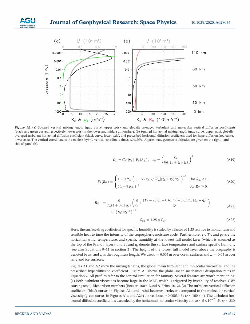
CD ¼ CN vLj j FLðRiLÞ ; cN ¼ ka

lnððzL þ zrÞ=zrÞ

� �2

(A19)

FLðRiLÞ ¼1 − 9 RiL 1þ 75 cN

ffiffiffiffiffiffiffiffiffiffiffiffiffiffiffiffiffiffiffiffiffiffiffiffiffiffiffiffiffiffiffiffiffiffi

jRiLjðzL þ zrÞ=zrp

�

−1

for RiL < 0

ð 1þ 9 RiL Þ−1 for RiL ≥ 0:

8

<

:

(A20)

RiL ¼ g

TLð1þ 0:61 qpÞg

cpþ ðTL − TsÞð1þ 0:61 qLÞþ0:61 TL ðqL − qsÞ

zL

� �

× v 2L =zL

2� �

−1

(A21)

CDq ¼ 1:25 × CD: (A22)

Here, the surface drag coefficient for specific humidity is scaled by a factor of 1.25 relative to momentum and

sensible heat to tune the intensity of the tropospheric moisture cycle. Furthermore, vL, TL, and qL are the

horizontal wind, temperature, and specific humidity at the lowest full model layer (which is assumed as

the top of the Prandtl layer), and Ts and qs denote the surface temperature and surface specific humidity

(see also Equations 9–11 in section 2). The height of the lowest full model layer above the orography is

denoted by zL, and zr is the roughness length. We use zr ¼ 0:005m over ocean surfaces and zr ¼ 0:05m over

land and ice surfaces.

Figures A1 and A2 show the mixing lengths, the global mean turbulent and molecular viscosities, and the

prescribed hyperdiffusion coefficient. Figure A3 shows the global‐mean mechanical dissipation rates in

Equation 2. All profiles refer to the control simulation for January. Several features are worth mentioning:

(1) Both turbulent viscosities become large in the MLT, which is triggered by instability of resolved GWs

causing small Richardson numbers (Becker, 2009; Lund & Fritts, 2012). (2) The turbulent vertical diffusion

coefficient (black curves in Figures A1a and A2a) becomes irrelevant compared to the molecular vertical

viscosity (green curves in Figures A1a and A2b) above about ∼ 0.0003 hPa (z ∼ 100 km). The turbulent hor-

izontal diffusion coefficient is exceeded by the horizontal molecular viscosity above ∼ 5 × 10−7 hPa (z ∼ 230

Figure A1. (a) Squared vertical mixing length (gray curve, upper axis) and globally averaged turbulent and molecular vertical diffusion coefficients

(black and green curves, respectively, lower axis) in the lower and middle atmosphere. (b) Squared horizontal mixing length (gray curve, upper axis), globally

averaged turbulent horizontal diffusion coefficient (black curve, lower axis), and prescribed horizontal diffusion coefficient used for hyperdiffusion (red curve,

lower axis). The vertical coordinate is the model's hybrid vertical coordinate times 1,013 hPa. Approximate geometric altitudes are given on the right‐hand

side of panel (b).



km, black and blue curves in Figure A2b). (3) The dissipation rate from hyperdiffusion (red curves in

Figure A3) is negligible compare to the dissipation rates from turbulent and molecular viscosities at all

altitudes (black and green solid curves in Figure A3). (4) The dissipation from macroturbulent horizontal

and vertical momentum diffusion is mainly due to small scales (horizontal wavelengths shorter than

2,000 km, cf. the solid to the dashed curves in Figure A3a). (5) Horizontal momentum diffusion from

molecular viscosity mainly dissipates the small scales, whereas molecular vertical momentum diffusion

mainly dissipates large horizontal scales (horizontal wavelengths larger than 2,000 km, cf. the solid to the

dashed curves in Figure A3b). (6) Ion drag is the predominant dissipation mechanism above ∼ 200 km

(blue curve in Figure A3b). The corresponding dissipation is mainly due to the large scales (not shown).

Figure A3. Gobal mean mechanical dissipation rates during January from different processes (see Equations 1 and 2). Black curves: turbulent plus molecular

horizontal momentum diffusion; red curves: hyperdiffusion of momentum; green curves: turbulent plus molecular vertical momentum diffusion; blue curve:

ion drag. Solid curves show the contributions from horizontal wavenumbers (n ≤ 240), while dashed curves show the corresponding contributions from

the large scales only (n ≤ 20). The vertical coordinate is the model's hybrid vertical coordinate times 1,013 hPa. Approximate geometric altitudes are

given on the right‐hand side of each panel.

Figure A2. Same as Figure A1 but for the thermosphere. Panel (b) includes the globally averaged molecular viscosities used for vertical and horizontal

diffusion (green and blue curves, respectively, lower axis).



Appendix B: Nonhydrostatic CorrectionIn the following we derive a nonhydrostatic correction of the geopotential, Φnh, which is added to the hor-

izontal momentum equation of the HIAMCM (see Equation 1). Our method follows Klingbeil and

Burchard (2013) who extended a hydrostatic estuarine circulation model by including nonhydrostatic

effects. Similar methods were also developed for atmospheric circulation models (e.g., Janjic et al., 2001).

Neglecting viscosity in the vertical momentum equation with z as vertical coordinate, the material vertical

acceleration, _w, is due to the nonhydrostatic pressure force (the gravity acceleration is canceled by the hydro-

static pressure force). In the vertical coordinate system of the HIAMCM, the nonhydrostatic vertical pressure

force can be expressed in terms of the nonhydrostatic geopotential as −∂ηΦnh/∂ηz, hence,

_w ¼ −∂ηΦnh = ∂ηz: (B1)

We assume that nonhydrostatic effects are not relevant in the troposphere. Therefore, Φnh is computed only

for altitudes where bðηÞ ¼ 0, which is equivalent to p ¼ aðηÞ (see section 2). We use b ¼ 0 for η < η1 ¼ 0:09,

corresponding to an altitude of z ∼ 15 km above which nonhydrostatic effects are included. We furthermore

use (see also Equation 8 in section 2)

w ≈ −

R T

p g_η ∂ηp ¼ −

R T

p g_p ¼ R T

p g

Z

η

0

ϑ ∂~ηp d~η for η < η1; (B2)

where ϑ ¼ ∇ · v . Combining Equations B2 and B1 leads to

Φnh ¼ −

Z

η1

η

R T

p g_w ∂~ηp d~η ≈

Z

η1

η

R T

p g

� �2

€p ∂~ηp d~η or (B3)

Φnh ¼ −

Z

η1

η

R T

p g

� �2

_p ϑþZ

~η

0

∂tϑ ∂ηp dη þ v ·

Z

~η

0

∇ϑ ∂ηp dη

0

@

1

A ∂~ηp d~η (B4)

for η< η1, which is used in the HIAMCM. Here, the time derivative (tendency) of the horizontal diver-

gence, ∂tϑ, is computed from the previous time step.

Appendix C: Moist Convection and Large‐Scale Condensational HeatingThe moisture cycle in the HIAMCM employs a simplified convection scheme that relaxes the temperature

and specific humidity to reference values that correspond to piecewise moist‐adiabatic profiles (depending

on the actual temperature and water vapor content in the column). To define these profiles, we recall that

moist convection and nonconvective condensation take place in only limited areas compared to a grid box

of a GCM. Hence, condensation or convection will take place before the saturation or moist instability level

is met. Furthermore, convective updrafts are surrounded by compensating subsidence of water vapor, as

well as by convective downdrafts with reevaporation of cloud water. To roughly represent these effects,

we specify the reference specific humidity as

qr ¼qsatðp; TÞ rðTÞ if qsatðp; TÞ rðTÞ < q

q else;

(C1)

where r (T) is defined as

r Tð Þ ¼

0:83 if T > T2 ¼ 285 K

0:71 if T < T1 ¼ 220 K

0:83 − 0:12 cos2π

2

T − T1

T2 − T1

� �

else:

8

>

>

>

<

>

>

>

:

1

C

C

C

A

(C2)

The saturation water vapor mass mixing ratio is given by the integrated Clausius‐Clapeyron equation:



qsatðT; pÞ ¼R

Rv

pref

pexp

ℓ

Rv

1

Tref

−

1

T

� ��

: (C3)

Here, R ¼ 287 m2 s−2K−1 and Rv ¼ 461 m2 s−2K−1 denote the gas constants of dry air (in the lower atmo-

sphere) and water vapor, respectively; pref ¼ 6:11 hPa and Tref ¼ 273 K are reference values, and

ℓ ¼ 2:5 × 106 m2 s−2 is the latent heat of water vapor per unit mass. The surface humidity, qs, is defined as

qs ¼ f s qsat Ts; psð Þ; (C4)

where f s ¼ f sðλ; ϕÞ is a prescribed relative surface humidity. The reference temperature, Tr, used in the

convection scheme is computed piecewise using

Tr ¼ T1 −Φ − Φ1

cp−

ℓ ð qr − qr1 Þcp

f or Tr ≥ T: (C5)

We start withT1 ¼ TL, where TL is the temperature at the lowest full model layer, then compute Tr at greater

heights from Equation C5 until the condition Tr< T is met; the temperature T at this level is then defined as

the new T1 from which the computation of Tr according to Equation C5 in continued, and so forth; the com-

putation of Tr is terminated at η ¼ 0:09 (corresponding to ∼ 90 hPa), which is the uppermost level at which

moist convection and large‐scale condensation are considered.

The relaxation rates used in the moist convection scheme follow the mass flux method of Kuo (1965): The

moisture subject to convective condensation corresponds to that transported into the air column by advec-

tion and diffusion. Moist convection is assumed to reach up to the highest level where the actual temperature

falls below the reference temperature. Denoting this level by the symbol ηc, the moisture supply into the con-

vective column is

_M ¼Z 1

ηc

−v ·∇q − _η ∂ηqþ1

∂ηp∇ · Kh ∂ηp ∇q� �

þ g

∂ηp∂η

ρ2g

∂ηpKz∂ηq

� ��

∂ηp

gdη: (C6)

The corresponding convective condensation and heating rates in Equations 3 and 2 are formulated as

relaxation:

Qconv ¼ cp αT ð Tr − T Þ (C7)

Cconv ¼ αq ð qr − q Þ ; (C8)

where the relaxation rates are determined from mass and energy conservation:

αT ¼ ℓ

cp_M

Z 1

ηc

ð Tr − T Þ ∂ηp

gdη

!

−1

(C9)

αq ¼ _M

Z 1

ηc

ð qr − q Þ ∂ηp

gdη

!

−1

: (C10)

Between ηc andη0 ¼ 0:09(corresponding to∼ 90 hPa) large‐scale condensation in terms of relaxation toward

the reference specific humidity is applied. This yields the following condensation and latent heating rates

used in Equations 2 and 3 in section 2:

Clarge ¼−αlarge ð qr − q Þ if ηc < η < η0 and q > qr

0 else

(C11)

Qlarge ¼ ℓ Clarge: (C12)

Here, the relaxation rate is αlarge= (30min)−1. In addition, the water vapor mixing is relaxed to 0 with a time

constant of 365 days everywhere, ensuring reasonable water vapor mixing ratios above the tropopause.



Appendix D: Thermodynamic Relations for Variable Gas ConstantThe assumption of a fixed gas constant for the dry phase of air is appropriate in the lower and middle atmo-

sphere, where N2 and O2 are dominant and well mixed. In the lower thermosphere, however, N2, O2, and O

are approximately equally dominant and are demixed (have different density scale heights). At about 200

km ≤z ≤ 400 km, O is dominant. At higher altitudes, He and then H become the dominant constituents.

Thus, atomic oxygen is the major constituent in the F region. The overall result is a significant increase of

the resultant gas constant, R, and of the specific heat per unit mass at constant density, cv, with increasing

height (e.g., Vadas, 2007). In order to precisely simulate the full dynamics of the variable mixture of the neu-

tral gas components in the thermosphere, one has to apply multiphase hydrodynamics (e.g., Del Genio

et al., 1979). On the other hand, a dynamical core of a GCM usually solves fluid dynamical equations for a

single phase. Hence, it is an issue to extend the dynamical core of a GCM into the thermosphere.

Different approaches are applied in different thermosphere‐ionosphere models (e.g., H.‐L. Liu et al., 2018).

The HIAMCM uses sensible heat as prognostic thermodynamic variable, as is usual in many GCMs. In the

following we show that in this case the model equations can consistently be extended into the thermosphere

by invoking functional dependencies of the form R ¼ RðpÞ and cp= cp(T).

Consider an air parcel in local thermodynamic equilibrium that consists of different components (or phases)

denoted by the index n. For each phase, the equation of state ispn ¼ RnρnT, and the internal energy and sen-

sible heat per unit mass can be written as en ¼ cvnT and hn ¼ en þ pn=ρn ¼ cpnT, respectively. Here cvn and

cpn ¼ cvn þ Rn are the specific heat capacities per unit mass at constant density and constant pressure for

each phase. Defining the mass mixing ratios for each phase as qn ¼ ρn=ρwith ρ ¼ ∑

nρn, the equation of state,

and the internal energy and sensible heat per unit mass of the air parcel can be written like the correspond-

ing relations for the individual phases:

∑

npn ¼ p ¼ ρ R T ; R ¼ ∑

nqn Rn (D1)

∑

nqn en ¼ e ¼ cv T ; cv ¼

∑

nqn cvn (D2)

∑

nqn hn ¼ h ¼ cp T; cp ¼

∑

nqn cpn ¼ cv þ R: (D3)

However, the differentials of the thermodynamic potentials for the air parcel lead to more complicated

expressions than for the individual phases. For example, the differential of internal energy reads after a

few steps:

de ¼ ∑

nðqn den þ en dqnÞ ¼

p

ρ2dρþ T dsþ ∑

ngn dqn: (D4)

Here, s ¼ ∑

nqnsn is the entropy per unit mass of the air parcel, sn is the entropy per unit mass of phase n, and

gn ¼ hn − T sn is the Gibbs free energy of phase n. Likewise, the differential of sensible heat of the air parcel

becomes

dh ¼ ∑

nðqn dhn þ hn dqnÞ ¼

dp

ρþ T dsþ ∑

ngn dqn: (D5)

Equations D4 and D5 imply that using the internal energy or the sensible heat of the air parcel as a prognos-

tic thermodynamic variable requires the knowledge of∑ngndqn. It is therefore not straightforward to extend

a GCM into the thermosphere and account for the variable gas constant and heat capacities in a thermody-

namically consistent way. In the following we propose a simple solution to this problem.

The thermodynamic differential of sensible heat for a single phase,

dh ¼ 1

ρdpþ T ds ¼ 1

ρdpþ T

∂s

∂p

� �

T

dpþ T∂s

∂T

� �

p

dT (D6)

yields for the second derivatives



∂2h

∂T ∂p¼ −

1

ρ2∂ρ

∂T

� �

p

þ ∂s

∂p

� �

T

þ T∂2s

∂T ∂p;

∂2h

∂p ∂T¼ T

∂2s

∂p ∂T: (D7)

These two expression must be equal; hence,

∂s

∂p

� �

T

¼ 1

ρ2∂ρ

∂T

� �

p

: (D8)

Using the ideal gas law with R ¼ RðpÞ, this leads to

∂s

∂p

� �

T

¼ −

R

pf or R ¼ RðpÞ: (D9)

The same expression is obtained if R is constant. However, if we allow R to be dependent on both pressure

and temperature, the situation would become more complex:

∂s

∂p

� �

T

¼ −

R

p−

T

p

∂R

∂T

� �

p

for R ¼ Rðp; TÞ: (D10)

Plugging Equation D9 or D10 back into Equation D6 and substituting 1/ρ in the first term on the rhs by the

ideal gas law, we get

dh ¼ T∂s

∂T

� �

p

dT for R ¼ RðpÞ (D11)

dh ¼ T∂s

∂T

� �

p

dT −

T

R ρ

∂R

∂T

� �

p

dp for R ¼ Rðp; TÞ: (D12)

Hence, only for R ¼ RðpÞ is the differential of the sensible heat proportional to the differential of the

temperature:

dh ¼ cp dT for R ¼ RðpÞ ; (D13)

where

cp ¼ T∂s

∂T

� �

p

(D14)

is the heat capacity per unit mass at constant pressure. Because of Equation D13, the sensible heat is a

function of the temperature alone and the heat capacity at constant pressure can only be a function of

the temperature:

cp ¼ cpðTÞ for R ¼ RðpÞ: (D15)

The implication of this analysis is that by specifyingR ¼ RðpÞand cp= cp(T), a GCMwith sensible heat as the

prognostic thermodynamic variable can consistently be extended into the thermosphere. Indeed, the equa-

tions of motion of the HIAMCM as specified in section 2 are thermodynamically and energetically consistent

for the whole model domain for R ¼ RðpÞ and cp= cp(T).

Our specification of R(p) and cp(T) in the HIAMCM is based on the approximate formulas given in

Vadas (2007) for R and γ ¼ cp=cv based on results from the TIME‐GCM. In the following we recapitulate

these formulas and show how they are used to construct the functions R(p) and cp(T). We define a reference

temperature, TR(p), corresponding to active solar conditions as (Profile II in Figure 1 of Vadas, 2007):

TR ¼

T1 ¼ 290 K if p > p1 ¼ 0:01 hPa

T2 ¼ 1000 K if p < p2 ¼ 7 × 10−9 hPa

T1 þ ðT2 − T1Þ sin2 π

2

lnp1 − ln p

lnp1 − lnp2

� �

else:

8

>

>

>

<

>

>

>

:

(D16)



The corresponding profile of R(p) is computed iteratively. We first set RðpÞ ¼ R1 ¼ 286:04 m2 s−2K−1 and

compute a reference density profile according to ρRðpÞ ¼ p=ð RðpÞ TRðpÞ Þ . We then use Equation 3 in

Vadas (2007) to compute the first iteration of R(p):

RðpÞ ¼ max R1 ; X−1MW × 8314:5 m2 s−2 K−1

� �

XMW ¼ XMW1 − XMW2

21 − tanh −

ln ρRðpÞ= g m−3ð Þð Þ þ 14:9

4:2

� ��

þ XMW2:(D17)

Here, XMW is the mean molecular or atomic weight of the gas particles, and XMW1 ¼ 28:97 and XMW2 ¼ 16

are the tropospheric and thermospheric (z ∼ 400–450 km) values of XMW, respectively. The result from

Equation D17 is then used to update ρR(p), which in turn is used to iterate R(p) using Equation D17, and

so forth. This procedure converges after only a few iterations. As the next step we use Equation 4 from

Vadas (2007) to compute

γRðpÞ ¼1

2γ1 − γ2ð Þ 1 − tanh −

ln ρRðpÞ= g m−3ð Þð Þ þ 15:1

4

� ��

þ γ2 and (D18)

cpRðpÞ ¼ maxγRðpÞ

γRðpÞ−1RðpÞ ; cp1

� �

; (D19)

where γ1 ¼ 1:4004, γ2 ¼ 1:67, and cp1 = 1,004 m2 s−2K−1. Since the profile cpR(p) corresponds to the refer-

ence temperature profile, TR(p), these two profiles can be used to construct cp(T). This is done using a sim-

ple fit with Legendre polynomials:

cpðTÞ ¼ ∑7

n¼0

cn PnðζÞ with ζ ¼−1 if T < T1

þ1 if T > T2

2ðT − T1Þ=ðT2 − T1Þ−1 else:

8

>

<

>

:

(D20)

Figure D1. (a) Pressure dependence of the gas constant using Equation D17 (green curve, lower axis) using the reference temperature profile according to

Equation D16 (gray curve, upper axis). The black curve (lower axis) shows the reference profile of the heat capacity according to Equation D19, whereas the

thick red curve shows the polynomial fit according to Equation D20. (b) Simulated global‐mean temperature (upper axis) and heat capacity (lower axis) from

Equation D20 during January.



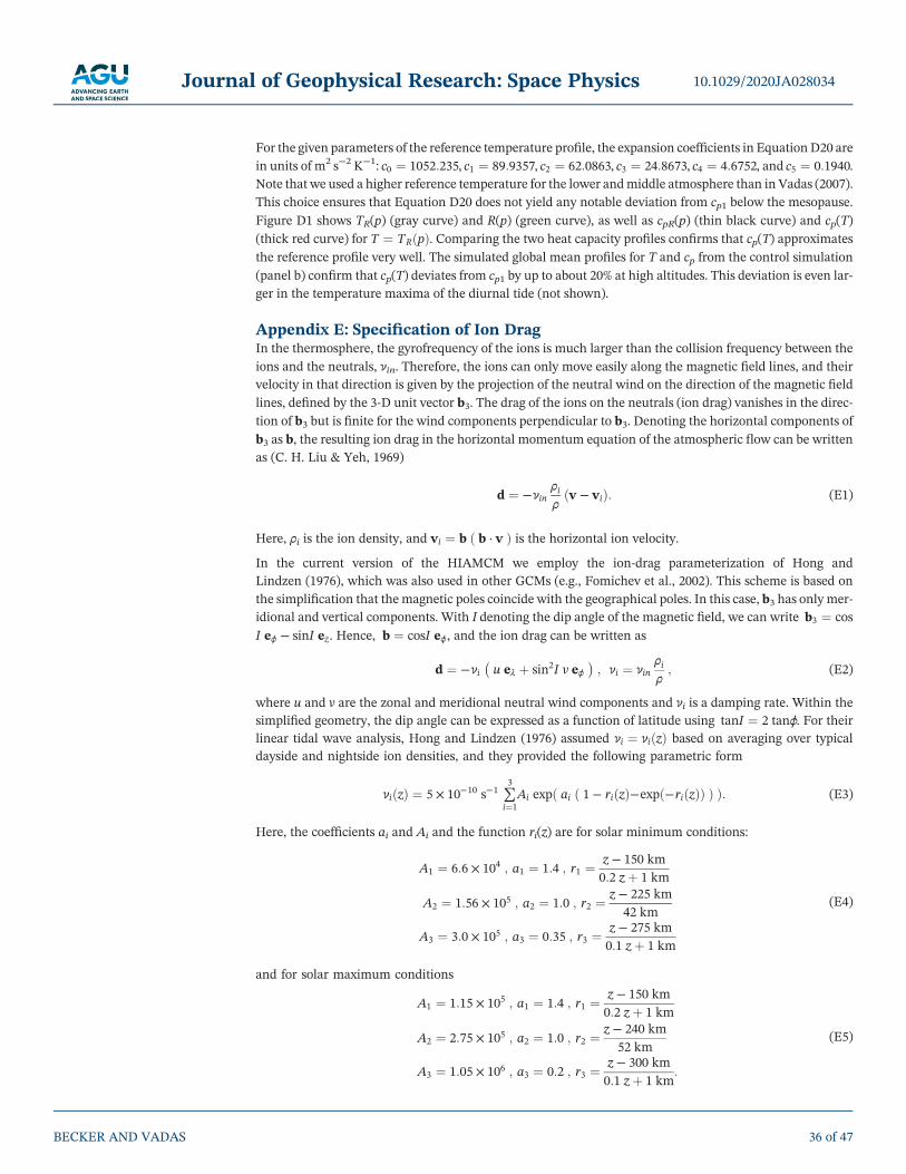
For the given parameters of the reference temperature profile, the expansion coefficients in EquationD20 are

in units of m2 s−2K−1: c0 ¼ 1052:235, c1 ¼ 89:9357, c2 ¼ 62:0863, c3 ¼ 24:8673, c4 ¼ 4:6752, and c5 ¼ 0:1940.

Note that we used a higher reference temperature for the lower andmiddle atmosphere than in Vadas (2007).

This choice ensures that Equation D20 does not yield any notable deviation from cp1 below the mesopause.

Figure D1 shows TR(p) (gray curve) and R(p) (green curve), as well as cpR(p) (thin black curve) and cp(T)

(thick red curve) for T ¼ TRðpÞ. Comparing the two heat capacity profiles confirms that cp(T) approximates

the reference profile very well. The simulated global mean profiles for T and cp from the control simulation

(panel b) confirm that cp(T) deviates from cp1 by up to about 20% at high altitudes. This deviation is even lar-

ger in the temperature maxima of the diurnal tide (not shown).

Appendix E: Specification of Ion DragIn the thermosphere, the gyrofrequency of the ions is much larger than the collision frequency between the

ions and the neutrals, νin. Therefore, the ions can only move easily along the magnetic field lines, and their

velocity in that direction is given by the projection of the neutral wind on the direction of the magnetic field

lines, defined by the 3‐D unit vector b3. The drag of the ions on the neutrals (ion drag) vanishes in the direc-

tion of b3 but is finite for the wind components perpendicular to b3. Denoting the horizontal components of

b3 as b, the resulting ion drag in the horizontal momentum equation of the atmospheric flow can be written

as (C. H. Liu & Yeh, 1969)

d ¼ −νinρiρðv − viÞ: (E1)

Here, ρi is the ion density, and vi ¼ b ð b · v Þ is the horizontal ion velocity.

In the current version of the HIAMCM we employ the ion‐drag parameterization of Hong and

Lindzen (1976), which was also used in other GCMs (e.g., Fomichev et al., 2002). This scheme is based on

the simplification that the magnetic poles coincide with the geographical poles. In this case, b3 has only mer-

idional and vertical components. With I denoting the dip angle of the magnetic field, we can write b3 ¼ cos

I eϕ − sinI ez. Hence, b ¼ cosI eϕ, and the ion drag can be written as

d ¼ −νi u eλ þ sin2I v eϕ� �

; νi ¼ νinρiρ; (E2)

where u and v are the zonal and meridional neutral wind components and νi is a damping rate. Within the

simplified geometry, the dip angle can be expressed as a function of latitude using tanI ¼ 2 tanϕ. For their

linear tidal wave analysis, Hong and Lindzen (1976) assumed νi ¼ νiðzÞ based on averaging over typical

dayside and nightside ion densities, and they provided the following parametric form

νiðzÞ ¼ 5 × 10−10 s−1 ∑3

i¼1

Ai exp ai 1 − riðzÞ−expð−riðzÞÞð Þð Þ: (E3)

Here, the coefficients ai and Ai and the function ri(z) are for solar minimum conditions:

A1 ¼ 6:6 × 104 ; a1 ¼ 1:4 ; r1 ¼z − 150 km

0:2 z þ 1 km

A2 ¼ 1:56 × 105 ; a2 ¼ 1:0 ; r2 ¼z − 225 km

42 km

A3 ¼ 3:0 × 105 ; a3 ¼ 0:35 ; r3 ¼z − 275 km

0:1 z þ 1 km

(E4)

and for solar maximum conditions

A1 ¼ 1:15 × 105 ; a1 ¼ 1:4 ; r1 ¼z − 150 km

0:2 z þ 1 km

A2 ¼ 2:75 × 105 ; a2 ¼ 1:0 ; r2 ¼z − 240 km

52 km

A3 ¼ 1:05 × 106 ; a3 ¼ 0:2 ; r3 ¼z − 300 km

0:1 z þ 1 km:

(E5)



For the simulations in this study, we applied this ion drag scheme for solar maximum conditions in the

following way. At each time step we compute the geometric height of the global‐mean temperature, T ,

according to

z ¼ ~z~z þ ae

ae; ~z ¼ g−1

Z

p00

p

RðpÞ T ðpÞp

dp ; (E6)

where ae is the Earth radius and p00 = 1,013 hPa. We then compute the damping rate as a function of

model layer (pressure in the thermosphere) from Equations E3 and E5. A dependence of the ion density

on the daily cycle is introduced using

νi → νi × 0:55þ 1:24 cosΘoð Þ (E7)

where Θo is the zenith angle of the solar insolation.

Appendix F: Radiation SchemeIn the following we describe idealized computation of radiative energy flux densities and associated heating

rates as implemented in the HIAMCM. These methods represent a further development of the previous

radiation scheme of the KMCM as described in Knöpfel and Becker (2011) and Becker et al. (2015).

F1. Shortwave Radiation

With So denoting the solar constant, we divide the solar insolation energetically into five bands according to

So ¼ ∑5

k¼1

Sko with Sko ¼ βk So: (F1)

Here, the βk describe the fractions of the solar insolation that are subject to absorption by ozone (β1 ¼ 0:0077

for UV‐C, β2 ¼ 0:225 for UV‐A and UV‐B) and by water vapor in the visible regime ( β3 ¼ 0:185 ).

Furthermore, the fraction β4 ¼ 7:6 × 10−6 is absorbed in the thermosphere, and β5 ¼ 1 − ∑ 4k¼1βk is subject

to absorption by tropospheric clouds. The eccentricity of the Earth's orbit around the Sun is accounted for by

specifying the solar constant as

So ¼ 1; 362 W m−2 þ cosð2πτÞ × 55 W m−2; (F2)

where τ denotes time in units of years. Using pressure p as vertical coordinate, the fluxes in the individual

bands are computed from Beer‐Bougert‐Lambert's law:

cos Θo

∂Sk

∂p¼ −g−1 ð ζ kΛk þ ζ 5 r Þ Sk with Skðp ¼ 0Þ ¼ cos Θo S

ko: (F3)

Here, Θo(λ, ϕ, t) is the zenith angle of solar insolation, where λ is longitude, ϕ is latitude, and t is univer-

sal time. The mass mixing ratios of the absorber gases are ζ 1 ¼ ζ 2 ¼ qO3 for ozone, ζ3= q for water vapor,

ζ 4 ¼ ðR2 − 0:7 RðpÞ−0:3 R1Þ=ðR2 − R1Þ (with R2 ¼ 570m2 s−2K−1 and R1 ¼ 286m2 s−2K−1) as an empiri-

cal representation of the mixture of air molecules and atomic oxygen in the thermosphere that give rise

to heating due to absorption of EUV radiation. Furthermore, ζ5 is a proxy for tropospheric clouds. We

use the relative humidity for this purpose but multiplied with a function fc that is unity between 800

and 300 hPa and approaches 0 from 300 to 100 hPa and a value of 0.3 below 800 hPa; hence ζ 5 ¼ f c q=

qsat . The reflection coefficient due to clouds is denoted by the symbol r in Equation F3. The shortwave

heating rates are computed according to

QkSW ¼ −g

ζ k Λk

ζ kΛk þ ζ 5 r∂pSk ; (F4)

and the reflected upward solar energy flux densities fulfill



∂Skor∂p

¼ −g−1 ζ 5 r

ζ kΛk

QkSW with Skorðp ¼ psÞ ¼ α Skoðp ¼ psÞ: (F5)

Here, α is a prescribed surface albedo having values of 0.04, 0.26, and 0.56 for ocean, land, and ice surfaces,

respectively. The band strengths, Λk, and the reflections coefficient are tunable parameters. In the present

model version we use the following values in units of m2 kg−1: Λ1 ¼ 3; 820, Λ2 ¼ 14:6, Λ3 ¼ 0:125, Λ4 ¼ 1

:1 × 104 , Λ5 ¼ 0:003, and r ¼ 8:85 × 10−4 . Global‐mean profiles of constituents and heating rates are pre-

sented in section F3.

F2. Longwave Radiation

Computation of the thermal radiation is based on the radiative transfer equation (e.g., Thomas &

Stamnes, 2002):

d Iν

d s¼ ρ κν −Iν þϖν

Z

Iν dΩ ð4πÞ−1 þ ð1 −ϖνÞ Bν

� �

: (F6)

Here, dΩ is the solid angle element, Iν is the intensity, κν is the mass extinction coefficient, and Bν is the

Planck function:

Bν ¼2 h ν3=c2

eh ν=kB T− 1

; (F7)

where h is the Planck constant, kB the Boltzman constant, and ν is the frequency in s−1. The

single‐scattering albedo, 0≤ϖν≤ 1, represents the effect of non‐LTE. Also note that

π

Z

∞

ν¼0

Bνdν ¼ σ T4 ; (F8)

where σ is the Stefan‐Boltzmann constant.

We assume a plane‐parallel and horizontally isotropic atmosphere, and we apply the Eddington approxima-

tion to parameterize the dependence of the intensity on the zenith angle,~ϑ. More specifically, Iν is assumed to

be independent of the horizontal direction, and its dependence on ~ϑ is parameterized using

Iν ¼Uν þ Dν

2πþ 3ðUν − DνÞ

4πcos~ϑ: (F9)

Here, Uν and Dν are the net upward and downward spectral energy flux densities; that is, Uν (−Dν) is the

solid‐angle integral of Iνcos~ϑ over the upper (lower) half sphere. Multiplying Equation F6 with cos~ϑ, using

dz ¼ dscos~ϑ, integrating over the upper and lower half sphere, and using pressure as vertical coordinate

by means of the hydrostatic formula yields the following transfer equations for the upward and downward

spectral energy flux densities (Knöpfel & Becker, 2011):

∂Uν

∂p¼ κν

g

7

4−ϖν

� �

Uν þ1

4−ϖν

� �

Dν − ð 2 − 2ϖν Þ π Bν

� �

(F10)

∂Dν

∂p¼ −

κνg

7

4−ϖν

� �

Dν þ1

4−ϖν

� �

Uν − ð 2 − 2ϖν Þ π Bν

� �

: (F11)

We now introduce six frequency bands: the 9.6 μm band of ozone (denoted by the index k ¼ 1), the 6.3 μm

water vapor band (k ¼ 2), the water vapor continuum (k ¼ 3), and three compartments of the 15 μm band of

carbon dioxide (k ¼ 4…6). An additional longwave extinction coefficient corresponds to an absorber in the

gray limit (index c). We associate this additional gray limit absorber with the longwave radiative effects of

tropospheric clouds and of NO in the mesopause region and lower thermosphere.

We use the decompositions



κν ¼ κk þ κ′ν ; κk ¼ 1

ν2k − ν1k

Z

ν2k

ν1k

κν dν (F12)

ðν2k − ν1kÞ Xν ¼ Xk þ X ′ν ; Xk ¼

Z

ν2k

ν1k

Xν dν ; (F13)

which are valid for each frequency band (i.e., for ν1k≤ ν≤ ν2k) and where X represents either U, D, or B.

Furthermore, ϖν is assumed to be independent of frequency for each band; hence,ϖν ¼ ϖk (defined at the

end of this section). With these definitions we integrate Equations F10 and F11 over frequency. Due to the

strong variations of κν, Uν, and Dν with frequency, the frequency‐integrated radiative transfer equations

include covariance terms of the form ‾κ′νD′ν and ‾κ′νU

′ν . These terms become important when the fre-

quency band consists of sharp instead of broad lines. In particular, the saturation in the CO2 15 μm band

is strongly dependent on the reduction of line broadening in the upper troposphere (Pierrehumbert, 2011).

Covariance terms of the form ‾κ′νB′ν are negligible because the Planck function varies only slowly with

frequency.

Since water vapor is mainly relevant in the troposphere, while the longwave radiative transfer of ozone is

important only in the stratosphere and lower mesosphere, and since saturation effects for these absorbers

are not important, we neglect the covariance terms for these bands and solve the following transfer equa-

tions for k ¼ 1–3:

∂Uk

∂p¼

7

4− ωk

gðκk þ κcÞ Uk þ

1

4− ωk

gðκk þ κcÞ Dk

−

2 − 2ωk

gðκk þ κcÞ π Bk (F14)

∂Dk

∂p¼ −

7

4− ωk

gðκk þ κcÞ Dk

−

1

4− ωk

gðκk þ κcÞ Uk þ 2 − 2ωk

gðκk þ κcÞ π Bk: (F15)

Here, κk ¼ Sk ςk , where the band strengths, Sk, are tunable parameters and ςk represents the mass mixing

ratio of ozone (k ¼ 1) and water vapor (k ¼ 2 and k ¼ 3): ς1 ¼ qO3 and ς2 ¼ ς3 ¼ q. The band strengths

and frequency ranges applied in the HIAMCM are given in the first three rows of Table 1.

The longwave effects of tropospheric clouds and NO are represented in a simplistic fashion using

κc ¼ Sc f c q=qsat þ SNO qNO: (F16)

Here, fc q/qsat is the cloud proxy defined in Appendix F1, Sc ¼ 0:0092 , SNO ¼ 0:2 , and the prescribed ver-

tical profile of the assumed mass mixing ratio qNO is given in Figure F1a (see Appendix F3).

The CO2 15 μmband is split into three wings (frequency compartments,k ¼ 4…6). These wings represent the

center of the band that has the strongest lines (k ¼ 5), as well the two wings next to the center at lower fre-

quencies (k ¼ 4 ) and at higher frequencies k ¼ 6 ). As discussed by Pierrehumbert (2011, see also his

Figure 2), the extinction coefficient varies strongly with frequency within each wing. The CO2 band includes

further wings, which are orders of magnitude weaker and therefore not very important, even though they

are relevant for the climate sensitivity to multiple CO2 doubling (Pierrehumbert, 2011). Since the infrared

radiative transfer calculations in the HIAMCM extend continuously from the surface to the model top,

and since CO2 is relevant at all altitudes up to the lower thermosphere, we must include the frequency var-

iations of the extinction coefficient within each wing k ¼ 4…6 to compute the frequency‐averaged upward

and downward spectral energy flux densities with sufficient accuracy. We found that the method proposed

in Knöpfel and Becker (2011) was not sufficient in this respect. In the following we propose a pseudo line‐by‐

line integration method.

A close inspection of the individual line strengths of the CO2 15 μm band based on the HITRAN data base

(Rothman et al., 2013) showed that each wing k ¼ 4…6 consists of two categories of lines, namely, very weak

lines and strong lines. The latter mainly account for the frequency‐averaged absorption coefficient in each



wing. For these strong lines we use the HITRAN data base to compute (1) the extinction coefficient as a func-

tion of frequency and (2) the parameters that determine the line widths as functions of pressure and tem-

perature. We then compute averaged values for these parameters. More specifically, each line is

parameterized with the Voigt profile, which includes Doppler and pressure broadening. The half‐line width

for a Voigt profile is given by (e.g., Thomas & Stamnes, 2002)

γV ¼ 0:5346 γL þffiffiffiffiffiffiffiffiffiffiffiffiffiffiffiffiffiffiffiffiffiffiffiffiffiffiffiffiffiffi

0:2166 γ2L þ γ2G

q

(F17)

γL ¼ T0

T

� �nk

γair p−100 ð p − pCO2 ÞþγCO2 p−1

00 pCO2� �

(F18)

γG ¼ ν02 ðln2Þ kBTc2mCO2

� �1=2

(F19)

where γL and γG are the line widths due to pressure broadening (with respect to a Lorentz line profile) and

Doppler broadening (with respect to a Gaussian line profile), respectively. The unit in these equations is

cm−1, as is convenient in radiative transfer computations. Furthermore, T0 ¼ 296 K, p00 = 1,013 hPa,

pCO2 is the partial pressure of CO2,mCO2 is the mass of the CO2 molecule in kg, and c is the speed of light.

The Lorentz line width, γL, comprises the pressure broadening from collisions with both air molecules and

CO2 molecules. Other parameters used in Equations F17–F19 are given in rows 4–6 of Table 1. Using these

numbers, Equations F17–F19 yield the mean half‐line widths, γkV ðp; TÞ, for each of the three central wings

(frequency compartments) of the CO2 15 μm band. Likewise, we also compute the averaged absorption

coefficients, κk, and line distances, δk (see Table 1).

We now assume that each wing can be approximated by the Elsasser band model (e.g., Thomas &

Stamnes, 2002, Chapter 10.3):

κð~ν; δk; ykÞ ¼ κk f Eð~ν; δk; ykÞ ; f E ¼ sinhð2πykÞcoshð2πykÞ−cosð2π~ν=δkÞ

: (F20)

Here, f Eð~ν; δk; ykÞ is the Elasser form function, yk ¼ γkV=δk is the grayness parameter, and ~ν is the frequency

in units of cm−1 (~ν ¼ ν=ð100 cÞ). This simple band model allows us to perform a pseudo line‐by‐line integra-

tion of Equations F10 and F11. To this end we discretize the frequency interval [ ~νk0 ; … ; ~νk0 þ δk=2 ], where

~νk0 can be chosen such that cosð2π~νk0=δkÞ ¼ 1. We define x ¼ 2π~ν=δk − 2π~νk0=δk and solve the radiative trans-

fer equations for discrete values of xi between x ¼ 0 and x ¼ π, multiplied by the corresponding Δxi. The

results from these spectral elements are then added and multiplied by 2Nk, where Nk is the number of lines

in the wing. This way we obtain the total energy flux density for each wing k ¼ 4…6. We discretize the inter-

val x ¼ 0…π by 20 frequencies on an irregular grid, with Δxi being smallest near x ¼ 0 to ensure that the limit

of sharp lines (small grayness parameter) is well resolved. Summarizing, the discrete radiative transfer equa-

tions that are solved for each spectral element i ¼ 1…20 in each wing k ¼ 4…6 are

∂Uki

∂p¼

7

4− ωk

gðκki þ κcÞ Uk

i þ1

4− ωk

gðκki þ κcÞ Dk

i −2 − 2ωk

gðκki þ κcÞ π Bk

i (F21)

∂Dki

∂p¼ −

7

4− ωk

gðκk þ κcÞ Dk

i −

1

4− ωk

gðκki þ κcÞ Uk

i þ2 − 2ωk

gðκki þ κcÞ π Bk

i : (F22)

which is analogous to Equations F14 and F15. Here,

Bki ¼

Δxki =π

2 NkBk

⇔ Bk ¼ 2 Nk ∑

i Bki ;

(F23)

and the extinction coefficients for each of the spectral elements are



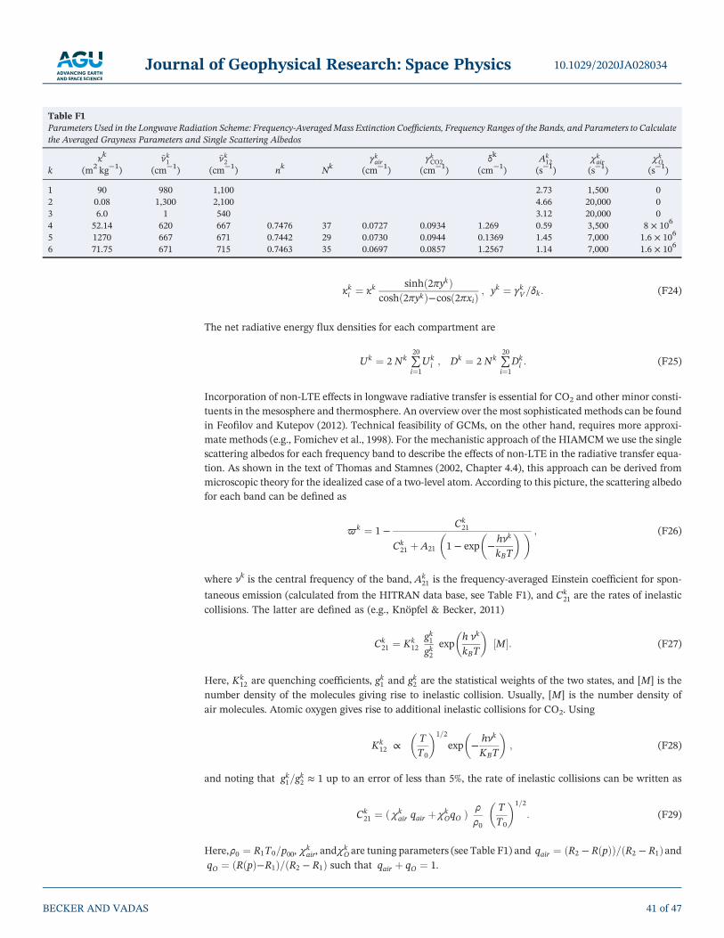
κki ¼ κksinhð2πykÞ

coshð2πykÞ−cosð2πxiÞ; yk ¼ γkV=δk: (F24)

The net radiative energy flux densities for each compartment are

Uk ¼ 2 Nk ∑20

i¼1

Uki ; Dk ¼ 2 Nk ∑

20

i¼1

Dki : (F25)

Incorporation of non‐LTE effects in longwave radiative transfer is essential for CO2 and other minor consti-

tuents in the mesosphere and thermosphere. An overview over the most sophisticated methods can be found

in Feofilov and Kutepov (2012). Technical feasibility of GCMs, on the other hand, requires more approxi-

mate methods (e.g., Fomichev et al., 1998). For the mechanistic approach of the HIAMCMwe use the single

scattering albedos for each frequency band to describe the effects of non‐LTE in the radiative transfer equa-

tion. As shown in the text of Thomas and Stamnes (2002, Chapter 4.4), this approach can be derived from

microscopic theory for the idealized case of a two‐level atom. According to this picture, the scattering albedo

for each band can be defined as

ϖk ¼ 1 −Ck21

Ck21 þ A21 1 − exp −

hνk

kBT

� �� ; (F26)

where νk is the central frequency of the band, Ak21 is the frequency‐averaged Einstein coefficient for spon-

taneous emission (calculated from the HITRAN data base, see Table F1), and Ck21 are the rates of inelastic

collisions. The latter are defined as (e.g., Knöpfel & Becker, 2011)

Ck21 ¼ Kk

12

gk1gk2

exph νk

kBT

� �

½M�: (F27)

Here, Kk12 are quenching coefficients, gk1 and gk2 are the statistical weights of the two states, and [M] is the

number density of the molecules giving rise to inelastic collision. Usually, [M] is the number density of

air molecules. Atomic oxygen gives rise to additional inelastic collisions for CO2. Using

Kk12 ∝

T

T0

� �1=2

exp −

hνk

KBT

� �

; (F28)

and noting that gk1=gk2 ≈ 1 up to an error of less than 5%, the rate of inelastic collisions can be written as

Ck21 ¼ ð χkair qair þ χkOqO Þ ρ

ρ0

T

T0

� �1=2

: (F29)

Here,ρ0 ¼ R1T0=p00, χkair, andχ

kO are tuning parameters (see Table F1) and qair ¼ ðR2 − RðpÞÞ=ðR2 − R1Þand

qO ¼ ðRðpÞ−R1Þ=ðR2 − R1Þ such that qair þ qO ¼ 1.

Table F1

Parameters Used in the Longwave Radiation Scheme: Frequency‐AveragedMass Extinction Coefficients, Frequency Ranges of the Bands, and Parameters to Calculate

the Averaged Grayness Parameters and Single Scattering Albedos

κk

~νk1 ~νk2 γkair γkCO2 δk

Ak12 χkair χkO

k (m2kg

−1) (cm

−1) (cm

−1) n

kNk

(cm−1

) (cm−1

) (cm−1

) (s−1

) (s−1

) (s−1

)

1 90 980 1,100 2.73 1,500 0

2 0.08 1,300 2,100 4.66 20,000 0

3 6.0 1 540 3.12 20,000 0

4 52.14 620 667 0.7476 37 0.0727 0.0934 1.269 0.59 3,500 8 × 106

5 1270 667 671 0.7442 29 0.0730 0.0944 0.1369 1.45 7,000 1.6 × 106

6 71.75 671 715 0.7463 35 0.0697 0.0857 1.2567 1.14 7,000 1.6 × 106



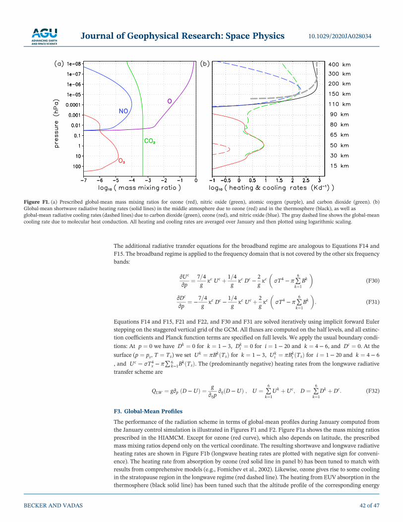
The additional radiative transfer equations for the broadband regime are analogous to Equations F14 and

F15. The broadband regime is applied to the frequency domain that is not covered by the other six frequency

bands:

∂Uc

∂p¼ 7=4

gκc Uc þ 1=4

gκc Dc

−

2

gκc σT4

− π∑6

k¼1

Bk

� �

(F30)

∂Dc

∂p¼ −

7=4

gκc Dc

−

1=4

gκc Uc þ 2

gκc σT4

− π∑6

k¼1

Bk

� �

: (F31)

Equations F14 and F15, F21 and F22, and F30 and F31 are solved iteratively using implicit forward Euler

stepping on the staggered vertical grid of the GCM. All fluxes are computed on the half levels, and all extinc-

tion coefficients and Planck function terms are specified on full levels. We apply the usual boundary condi-

tions: At p ¼ 0 we have Dk ¼ 0 for k ¼ 1 − 3, Dki ¼ 0 for i ¼ 1 − 20 and k ¼ 4 − 6, and Dc ¼ 0. At the

surface (p ¼ ps, T ¼ Ts) we set Uk ¼ πBkðTsÞ for k ¼ 1 − 3, Uki ¼ πBk

i ðTsÞ for i ¼ 1 − 20 and k ¼ 4 − 6

, and Uc ¼ σT4s − π∑ 6

k¼1BkðTsÞ. The (predominantly negative) heating rates from the longwave radiative

transfer scheme are

QLW ¼ g∂p ðD − UÞ ¼ g

∂ηp∂ηðD − UÞ ; U ¼ ∑

6

k¼1

Uk þ Uc; D ¼ ∑6

k¼1

Dk þ Dc: (F32)

F3. Global‐Mean Profiles

The performance of the radiation scheme in terms of global‐mean profiles during January computed from

the January control simulation is illustrated in Figures F1 and F2. Figure F1a shows the mass mixing ratios

prescribed in the HIAMCM. Except for ozone (red curve), which also depends on latitude, the prescribed

mass mixing ratios depend only on the vertical coordinate. The resulting shortwave and longwave radiative

heating rates are shown in Figure F1b (longwave heating rates are plotted with negative sign for conveni-

ence). The heating rate from absorption by ozone (red solid line in panel b) has been tuned to match with

results from comprehensive models (e.g., Fomichev et al., 2002). Likewise, ozone gives rise to some cooling

in the stratopause region in the longwave regime (red dashed line). The heating from EUV absorption in the

thermosphere (black solid line) has been tuned such that the altitude profile of the corresponding energy

Figure F1. (a) Prescribed global‐mean mass mixing ratios for ozone (red), nitric oxide (green), atomic oxygen (purple), and carbon dioxide (green). (b)

Global‐mean shortwave radiative heating rates (solid lines) in the middle atmosphere due to ozone (red) and in the thermosphere (black), as well as

global‐mean radiative cooling rates (dashed lines) due to carbon dioxide (green), ozone (red), and nitric oxide (blue). The gray dashed line shows the global‐mean

cooling rate due to molecular heat conduction. All heating and cooling rates are averaged over January and then plotted using logarithmic scaling.



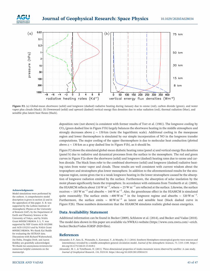
deposition rate (not shown) is consistent with former results of Torr et al. (1981). The longwave cooling by

CO2 (green dashed line in Figure F1b) largely balances the shortwave heating in the middle atmosphere and

strongly decreases above z ∼ 150 km (note the logarithmic scale). Additional cooling in the mesopause

region and lower thermosphere is simulated by our simple incorporation of NO in the longwave transfer

computations. The major cooling of the upper thermosphere is due to molecular heat conduction (plotted

above z ∼ 130 km as a gray dashed line in Figure F1b), as it should be.

Figure F2 shows the simulated global‐mean diabatic heating rates (panel a) and vertical energy flux densities

(panel b) due to radiative and dynamical processes from the surface to the mesosphere. The red and green

curves in Figure F2a show the shortwave (solid) and longwave (dashed) heating rates due to ozone and car-

bon dioxide. The black lines refer to the combined shortwave (solid) and longwave (dashed) radiative heat-

ing rates from water vapor and clouds. These results are well consistent with current wisdom about the

troposphere and stratosphere plus lower mesosphere. In addition to the aforementioned results for the stra-

topause region, ozone gives rise to a weak longwave heating in the lower stratosphere caused be the absorp-

tion of longwave radiation emitted by the surface. Furthermore, the absorption of solar insolation by the

moist phases significantly heats the troposphere. In accordance with estimates from Trenberth et al. (2009),

the HIAMCM reflects about 110Wm−2, where∼ 25Wm−2 are reflected at the surface. Likewise, the surface

receives ∼ 185Wm−2 and absorbs ∼ 160Wm−2. Also, the greenhouse effect in the HIAMCM is simulated

quite reasonably: The surface emits ∼400Wm−2 in the longwave regime and absorbs ∼ 320Wm−2.

Furthermore, the surface emits ∼ 80Wm−2 as latent and sensible heat (black dashed curve in

Figure F2b). These numbers demonstrate that the HIAMCM simulates realistic global‐mean energetics.

Data Availability Statement

Additional information can be found in Becker (2009), Schlutow et al. (2014), and Becker and Vadas (2018).

The model data shown in this paper are available via NWRA's website (https://www.cora.nwra.com/∼erich.

becker/BeckerVadas-JGRSP-2020-files).

ReferencesAlexander, S. P., Sato, K., Watanabe, S., Kawatani, Y., &Murphy, D. J. (2016). Southern Hemisphere extratropical gravity wave sources and

intermittency revealed by a middle‐atmosphere general circulation model. Journal of the Atmospheric Sciences, 73, 1335–1349. https://

doi.org/10.1175/JAS-D-15-0149.1

Alexander, M. J., & Teitelbaum, H. (2011). Three‐dimensional properties of Andes mountain waves observed by satellite: A case study.

Journal of Geophysical Research, 116, D23110. https://doi.org/10.1029/2011JD016151

Figure F2. (a) Global‐mean shortwave (solid) and longwave (dashed) radiative heating during January due to ozone (red), carbon dioxide (green), and water

vapor plus clouds (black). (b) Downward (solid) and upward (dashed) vertical energy flux densities due to solar radiation (red), thermal radiation (blue), and

sensible plus latent heat fluxes (black).



Acknowledgments

Model simulations were performed by

the authors. A comprehensive model

description is given in section 22 and in

the appendices of this paper. E. B. was

supported by the Leibniz Institute of

Atmospheric Physics at the University

of Rostock (IAP), by the Department of

Earth and Planetary Science at the

University of Tokyo, and by NASA

Grant 80NSSC19K0834. S. L. V. was

supported by NSF Grants AGS‐1832988

and AGS‐1552315 and by NASA Grant

80NSSC19K0836. We thank Kai Budde

for evaluating the HITRAN data.

Discussions with Richard Walterscheid,

Joe Huba, Douglas Drob, and Aaron

Riddley are gratefully acknowledged.

We thank two anonymous reviewers for

numerous helpful comments on the

manuscript.

Becker, E. (2003). Frictional heating in global climate models. Monthly Weather Review, 131, 508–520.

Becker, E. (2004). Direct heating rates associated with gravity wave saturation. Journal of Atmospheric and Solar‐Terrestrial Physics, 66,

683–696. https://doi.org/10.1016/j.jastp.2004.01.019

Becker, E. (2009). Sensitivity of the upper mesosphere to the Lorenz energy cycle of the troposphere. Journal of the Atmospheric Sciences, 66,

648–666. https://doi.org/10.1175/2008JAS2735.1

Becker, E. (2017). Mean‐flow effects of thermal tides in the mesosphere and lower thermosphere. Journal of the Atmospheric Sciences, 74,

2043–2063. https://doi.org/10.1175/JAS-D-16-0194.1

Becker, E., & Burkhardt, U. (2007). Nonlinear horizontal diffusion for GCMs. Monthly Weather Review, 135, 1439–1454.

Becker, E., Knöpfel, R., & Lübken, F.‐J. (2015). Dynamically induced hemispheric differences in the seasonal cycle of the summer polar

mesopause. Journal of Atmospheric and Solar‐Terrestrial Physics, 129, 128–141. https://doi.org/10.1016/j.jastp.2015.04.014

Becker, E., & Vadas, S. L. (2018). Secondary gravity waves in the winter mesosphere: Results from a high‐resolution global circulation

model. Journal of Geophysical Research: Atmospheres, 123, 2605–2627. https://doi.org/10.1002/2017JD027460

Bossert, K., Fritts, D. C., Williams, B. P., Kruse, C. G., Healea, C. J., Pautet, P.‐D., et al. (2017). Secondary gravity wave generation over New

Zealand during the DEEPWAVE campaign. Journal of Geophysical Research: Atmospheres, 122, 7834–7850. https://doi.org/10.1002/

2016JD026079

Brune, S., & Becker, E. (2013). Indications of stratified turbulence in a mechanistic GCM. Journal of the Atmospheric Sciences, 70, 231–247.

https://doi.org/10.1175/JAS-D-12-025.1

Chen, C., & Chu, X. (2017). Two‐dimensional Morlet wavelet transform and its application to wave recognition methodology of automa-

tically extracting two‐dimensional wave packets from lidar observations in Antarctica. Journal of Atmospheric and Solar‐Terrestrial

Physics, 162, 28–47. https://doi.org/10.1016/j.jastp.2016.10.016

Chen, C., Chu, X., McDonald, A. J., Vadas, S. L., Yu, Z., Fong, W., & Lu, X. (2013). Inertia‐gravity waves in antarctica: A case study using

simultaneous lidar and radar measurements at McMurdo/Scott Base (77.8°S, 166.7°E). Journal of Geophysical Research: Atmospheres,

118, 2794–2808. https://doi.org/10.1002/jgrd.50318

Chen, C., Chu, X., Zhao, J., Roberts, B. R., Yu, Z., Fong, W., et al. (2016). Lidar observations of persistent gravity waves with periods of 3–10

h in the Antarctic middle and upper atmosphere at McMurdo (77.83°S, 166.67°E). Journal of Geophysical Research: Space Physics, 121,

1483–1502. https://doi.org/10.1002/2015JA022127

Crowley, G., Jones, T. B., & Dudeney, J. R. (1987). Comparison of short period TID morphologies in Antarctica during geomagnetically

quiet and active intervals. Journal of Atmospheric and Solar‐Terrestrial Physics, 49, 1155–1162. https://doi.org/10.1016/0021-

9169(87)90098-5

Crowley, G., & Rodrigues, F. S. (2012). Characteristics of traveling ionospheric disturbances observed by the TIDDBIT sounder. Radio

Science, 47, RS0L22. https://doi.org/10.1029/2011RS004959

Dalgarno, A., & Smith, F. J. (1962). The thermal conductivity and viscosity of atomic oxygen. Planetary and Space Science, 9, 1–2. https://

doi.org/10.1016/0032-0633(62)90064-8

deWit, R. J., Janches, D., Fritts, D. C., Stockwell, R., & Coy, L. (2017). Unexpected climatological behavior of MLT gravity wave momentum

flux in the lee of the Southern Andes hotspot. Geophysical Research Letters, 44, 1182–1191. https://doi.org/10.1002/2016GL072311

Del Genio, A. D., Schubert, G., & Straus, J. M. (1979). Gravity wave propagation in a diffusively separated atmosphere with

height‐dependent collision frequencies. Journal of Geophysical Research, 84, 4371–4378. https://doi.org/10.1029/JA084iA08p04371

Drob, D. P., Emmert, J. T., Meriwether, J. W., Makela, J. J., Doornbos, E., Conde, M., et al. (2015). An update to the Horizontal Wind Model

(HWM): The quiet time thermosphere. Earth and Space Science, 2, 301–319. https://doi.org/10.1002/2014EA000089

Eckermann, S. D., & Preusse, P. (1999). Global measurements of stratospheric mountain waves from space. Science, 286, 1534–1536.

Ern, M., Trinh, Q. T., Kaufmann, M., Krisch, I., Preusse, P., Ungermann, J., et al. (2016). Satellite observations of middle atmosphere gravity

wave absolute momentum flux and of its vertical gradient during recent stratospheric warmings. Atmospheric Chemistry and Physics, 16,

9983–10,019. https://doi.org/10.5194/acp-16-9983-2016

Ern, M., Trinh, Q. T., Preusse, P., Gille, J. C., Mlynczak, M. G., Russell, J. M. III., & Riese, M. (2018). GRACILE: A comprehensive clima-

tology of atmospheric gravity wave parameters based on satellite limb soundings. Earth System Science Data, 10, 857–892. https://doi.

org/10.5194/essd-10-857-2018

Feofilov, A. G., & Kutepov, A. A. (2012). Infrared radiation in the mesosphere and lower thermosphere: Energetic effects and remote

sensing. Surveys in Geophysics, 33(6), 1231–1280.

Fleming, E. L., Chandra, S., Barnett, J. J., & Corney, M. (1990). Zonal mean temperature, pressure, zonal wind and geopotential height as

functions of latitude. Advances in Space Research, 10(12), 11–59. https://doi.org/10.1016/0273-1177(90)90386-E

Fomichev, V. I., Blanchet, J.‐P., & Turner, D. S. (1998). Matrix parameterization of the 15 μm CO2 band cooling in the middle and upper

atmosphere for variable co2 concentration. Journal of Geophysical Research, 103(11), 11,505–11,528.

Fomichev, V. I., Ward, W. E., Beagley, S. R., McLandress, C., McConnell, J. C., McFarlane, N. A., & Shepherd, T. G. (2002). Extended

Canadian Middle Atmosphere Model: Zonal‐mean climatology and physical parameterizations. Journal of Geophysical Research,

107(D10), ACL 9‐1–ACL 9‐14. https://doi.org/10.1029/2001JD000479

Forbes, J. M., Bruinsma, S. L., Doornbos, E., & Zhang, X. (2016). Gravity wave‐induced variability of the middle thermosphere. Journal of

Geophysical Research: Space Physics, 121, 6914–6932. https://doi.org/10.1002/2016JA022923

Frissell, N. A., Baker, J. B. H., Ruohoniemi, J. M., Greenwald1, R. A., Gerrard2, A. J., Miller, E. S., & West, M. L. (2016). Sources and

characteristics of medium‐scale traveling ionospheric disturbances observed by high‐frequency radars in the north american sector.

Journal of Geophysical Research: Space Physics, 121, 3722–3739. https://doi.org/10.1002/2015JA022168

Fritts, D. C., & Alexander, M. J. (2003). Gravity wave dynamics and effects in the middle atmosphere. Reviews of Geophysics, 41, 1003.

https://doi.org/10.1029/2001/RG000106

Fritts, D. C., Dong, W., Lund, T. S., Wieland, S., & Laughman, B. (2020). Self‐acceleration and instability of gravity wave packets: 3.

Three‐dimensional packet propagation, secondary gravity waves, momentum transport, and transient mean forcing in tidal winds.

Journal of Geophysical Research: Atmospheres, 125, e2019JD030692. https://doi.org/10.1029/2019JD030692

Fritts, D. C., Smith, R. B., Taylor, M. J., Doyle, J. D., Eckermann, S. D., Dörnbrack, A., et al. (2016). The Deep Propagating Gravity Wave

Experiment (DEEPWAVE): An airborne and ground‐based exploration of gravity wave propagation and effects from their sources

throughout the lower and middle atmosphere. Bulletin of the American Meteorological Society, 97(3), 425–453. https://doi.org/10.1175/

BAMS-D-14-00269.1

Fritts, D. C., & Vadas, S. L. (2008). Gravity wave penetration into the thermosphere: Sensitivity to solar cycle variations and mean winds.

Annales Geophysicae, 26, 3841–3861.



Fritts, D. C., Vadas, S. L., Wan, K., & Werne, J. A. (2006). Mean and variable forcing of the middle atmosphere by gravity waves. Journal of

Atmospheric and Solar‐Terrestrial Physics, 68, 247–265. https://doi.org/10.1016/j.jastp.2005.04.010

Gassmann, A. (2018). Entropy production due to subgrid‐scale thermal fluxes with application to breaking gravity waves.Quarterly Journal

of the Royal Meteorological Society, 144, 499–510. https://doi.org/10.1002/qj.3221

Gossard, E. E., & Hooke, W. H. (1975). Waves in the atmosphere (p. 112). New York: Elsivier.

Heale, C. J., Bossert, K., Vadas, S. L., Hoffmann, L., Dörnbrack, A., Stober, G., et al. (2020). Secondary gravity waves generated by breaking

mountain waves over europe. Journal of Geophysical Research: Atmospheres, 125, e2019JD031662. https://doi.org/10.1029/

2019JD031662

Heale, C. J., Walterscheid, R. L., & Snively, J. B. (2018). Localization effects on the dissipation of gravity wave packets in the upper

mesosphere and lower thermosphere. Journal of Geophysical Research: Atmospheres, 123, 8915–8935. https://doi.org/10.1029/2017/

JD027617

Hedin, A. E. (1991). Extension of the MSIS thermosphere model into the middle and lower atmosphere. Journal of Geophysical Research,

96(A2), 1159–1172.

Hendricks, E. A., Doyle, J. D., Eckermann, S. D., Jiang, Q., & Reinecke, P. A. (2014). What is the source of the stratopsheric gravity wave belt

in austral winter. Journal of the Atmospheric Sciences, 71, 1583–1592. https://doi.org/10.1175/JAS-D-13-0332.1

Hocke, K., & Schlegel, K. (1996). A review of atmospheric gravity waves and travelling ionospheric disturbances: 1982‐1995. Annales

Geophysicae, 14, 917–940.

Holtslag, A. A. M., & Boville, B. A. (1993). Local versus non‐local boundary‐layer diffusion in a global climate model. Journal of Climate, 6,

1825–1842.

Hong, S.‐S., & Lindzen, R. S. (1976). Solar semidiurnal tide in the thermosphere. Journal of the Atmospheric Sciences, 33, 135–153.

Howard, L. N. (1961). Note on a paper of John W. Miles. Journal of Fluid Mechanics, 10, 509–512.

Huang, K. M., Liu, A. Z., Zhang, S. D., Yi, F., Huang, C. M., Gong, Y., et al. (2017). Simultaneous upward and downward propagating

inertia‐gravity waves in the MLT observed at Andes Lidar Observatory. Journal of Geophysical Research: Atmospheres, 122, 2812–2830.

https://doi.org/10.1002/2016JD026178

Janjic, Z. I., Gerrity, J. P. Jr., & Nickovic, S. (2001). An alternative approach to nonhydrostatic modeling. Monthly Weather Review, 129,

1164–1178.

Jiang, J. H., Wu, D. L., & Eckermann, S. D. (2002). Upper Atmosphere Research Satellite (UARS) MLS observation of mountain waves over

the Andes. Journal of Geophysical Research, 107(D20), 8273. https://doi.org/10.1029/2002JD002091

Klingbeil, K., & Burchard, H. (2013). Implementation of a direct nonhydrostatic pressure gradient discretisation into a layered ocean

model. Ocean Modelling, 65, 64–77. https://doi.org/10.1016/j.ocemod.2013.02.002

Knöpfel, R., & Becker, E. (2011). An idealized radiative transfer scheme for use in a mechanistic general circulation model from the surface

up to the mesopause region. Journal of Quantitative Spectroscopy & Radiative Transfer, 112, 1460–1478. https://doi.org/10.1016/j.

jqsrt.2011.02.014

Kuo, H. L. (1965). On formation and intensification of tropical cyclones through latent heat release by cumulus convection. Journal of the

Atmospheric Sciences, 22, 40–63.

Lindzen, R. S. (1981). Turbulence and stress owing to gravity wave and tidal breakdown. Journal of Geophysical Research, 86, 9707–9714.

Liu, H.‐L. (2017). Large wind shears and their implications for diffusion in regions with enhanced static stability: The mesopause and the

tropopause. Journal of Geophysical Research: Atmospheres, 122, 9579–9590. https://doi.org/10.1002/2017JD026748

Liu, H.‐L., Bardeen, C. G., Foster, B. T., Lauritzen, P., Liu, J., Lu, G., et al. (2018). Development and validation of the Whole Atmosphere

Community Climate Model with thermosphere and ionosphere extension (WACCM‐X 2.0). Journal of Advances in Modeling Earth

Systems, 10, 381–402. https://doi.org/10.1002/2017MS001232

Liu, H.‐L., McInerney, J. M., Santos, S., Lauritzen, P. H., Taylor, M. A., & Pedatella, N. M. (2014). Gravity waves simulated by

high‐resolution Whole Atmosphere Community Climate Model. Geophysical Research Letters, 41, 9106–9112. https://doi.org/10.1002/

2014GL062468

Liu, X., Xu, J., Yue, J., Vadas, S. L., & Becker, E. (2019). Orographic primary and secondary gravity waves in the middle atmosphere from

16‐year SABER observations. Geophysical Research Letters, 46, 4512–4522. https://doi.org/10.1029/2019GL082256

Liu, C. H., & Yeh, K. C. (1969). Effect of ion drag on propagation of acoustic‐gravity waves in the atmospheric F region. Journal of

Geophysical Research, 74(2), 2248–2255.

Lübken, F.‐J. (1997). Seasonal variation of turbulent energy dissipation rates at high latitudes as determined by in situ measurements of

neutral density fluctuations. Journal of Geophysical Research, 102, 13,441–13,456.

Lund, T. S., & Fritts, D. C. (2012). Numerical simulation of gravity wave breaking in the lower thermosphere. Journal of Geophysical

Research, 117, D21105. https://doi.org/10.1029/2012JD017536

McLandress, C., Ward, W. E., Fomichev, V. I., Semeniuk, K., Beagley, S. R., McFarlane, N. A., & Shepherd, T. G. (2006). Large‐scale

dynamics of the mesosphere and lower thermosphere: An analysis using the extended Canadian Middle Atmosphere Model. Journal of

Geophysical Research, 111, D17111. https://doi.org/10.1029/2005JD006776

Miles, J. W. (1961). On the stability of heterogeneous shear flows. Journal of Fluid Mechanics, 10, 496–508.

Miyoshi, Y., Fujiwara, H., Jin, H., & Shinagawa, H. (2014). A global view of gravity waves in the thermosphere simulated by a general

circulation model. Journal of Geophysical Research: Space Physics, 119, 5807–5820. https://doi.org/10.1002/2014JA019848

Muraschko, J., Fruman, M. D., Achatz, U., Hickel, S., & Toledoc, Y. (2015). On the application of Wenzel‐Kramer‐Brillouin theory for the

simulation of the weakly nonlinear dynamics of gravity waves. Quarterly Journal of the Royal Meteorological Society, 141, 676–697.

https://doi.org/10.1002/qj.2381

Nicolls, M. J., Vadas, S. L., Aponte, N., & Sulzer, M. P. (2014). Horizontal wave parameters of daytime thermospheric gravity waves and E

region neutral winds over Puerto Rico. Journal of Geophysical Research: Space Physics, 119, 575–600. https://doi.org/10.1002/

2013JA018988

O'Sullivan, D., & Dunkerton, T. J. (1995). Generation of inertia‐gravity waves in a simulated life‐cycle of baroclinic instability. Journal of the

Atmospheric Sciences, 52, 3695–3716.

Olbers, D., Eden, C., Becker, E., Pollmann, F., & Jungclaus, J. (2019). The IDEMIX Model: Parameterization of internal gravity waves for

circulation models of ocean and atmosphere. In C. Eden & A. Iske (Eds.), Energy Transfers in Atmosphere and Ocean, Mathematics of

Planet Earth (Vol. 1, pp. 87–125). Cham: Springer. https://doi.org/10.1007/978-3-030-05704-6_3

Park, J., Lühr, H., Lee, C., Kim, Y. H., Jee, G., & Kim, J.‐H. (2014). A climatology of medium‐scale gravity wave activity in the

midlatitude/low‐latitude daytime upper thermosphere as observed by CHAMP. Journal of Geophysical Research: Space Physics, 19,

2187–2196. https://doi.org/10.1002/2013JA019705



Pierrehumbert, R. T. (2011). Infrared radiation and planetary temperature. Physics Today, 64(1), 33–38. https://doi.org/10.1063/1.3541943

Plougonven, R., & Zhang, F. (2014). Internal gravity waves from atmospheric jets and fronts. Reviews of Geophysics, 52, 33–76. https://doi.

org/10.1002/2012RG000419

Roble, R. G., & Ridley, E. C. (1994). A thermosphere‐ionosphere‐mesosphere‐electrodynamics general circulation model (time‐GCM):

Equinox solar cycle minimum simulations (30–500 km). Geophysical Research Letters, 21, 417–420.

Rothman, L. S., Gordon, I. E., Babikov, Y., Barbe, A., Benner, D. C., Bernath, P. F., et al. (2013). The HITRAN2012, molecular spectroscopic

database. Journal of Quantitative Spectroscopy & Radiative Transfer, 130, 4–50. https://doi.org/10.1016/j.jqsrt.2013.07.002

Sato, K., Tanteno, S., Watanabe, S., & Kawatani, Y. (2012). Gravity wave characteristics in the Southern Hemisphere revealed by a

high‐resolution middle‐atmosphere general circulation model. Journal of the Atmospheric Sciences, 69, 1378–1396. https://doi.org/

10.1175/JAS-D-11-0101.1

Sato, K., & Yoshiki, M. (2008). Gravity wave generation around the polar vortex in the stratosphere revealed by 3‐hourly radiosonde

observations at Syowa Station. Journal of the Atmospheric Sciences, 65, 3719–3735. https://doi.org/10.1175/2008JAS2539.1

Schaefer‐Rolffs, U., & Becker, E. (2018). Scale‐invariant formulation of momentum diffusion for high‐resolution atmospheric circulation

models. Monthly Weather Review, 146, 1045–1062. https://doi.org/10.1175/MWR-D-17-0216.1

Schlutow, M., Becker, E., & Körnich, H. (2014). Positive definite and mass conserving tracer transport in spectral GCMs. Journal of

Geophysical Research: Atmospheres, 119, 11,562–11,577. https://doi.org/10.1002/2014JD021661

Shibuya, R., Sato, K., Tsutsumi, M., Sato, T., Tomikawa, Y., Nishimura, K., & Kohma, M. (2017). Quasi‐12 h inertia‐gravity waves in the

lower mesosphere observed by the pansy radar at Syowa Station (39.6°E, 69.0°S). Atmospheric Chemistry and Physics, 17, 6455–6476.

https://doi.org/10.5194/acp-17-6455-2017

Simmons, A. J., & Burridge, D. M. (1981). An energy and angular momentum conserving vertical finite‐difference scheme and hybrid

vertical coordinates. Monthly Weather Review, 109, 758–766.

Smagorinsky, J. (1993). Some historical remarks on the use of nonlinear viscosities. In B. Galperin, & Orszag, A. St. (Eds.), Large eddy

simulation of complex engineering and geophysical flows (pp. 3–36). Cambridge: Cambridge University Press.

Smith, A. K. (2012). Global dynamics of the MLT. Surveys Geophysics, 33, 1177–1230. https://doi.org/10.1007/s10712-012-9196-9

Thomas, G. E., & Stamnes, K. (2002). Radiative Transfer in the Atmosphere and Ocean, Cambridge Atmospheric and Space Science Series

(p. 517). Cambridge: Cambridge University Press.

Torr, M. R., Richards, P. G., & Torr, D. G. (1981). Solar EUV energy budget of the thermosphere. Advances in Space Research, 1, 53–61.

https://doi.org/10.1016/0273-1177(81)90417-8

Trenberth, K. E., Fasullo, J. T., & Kiehl, J. (2009). Earth's global energy budget. Bulletin of the American Meteorological Society, 90, 311–323.

https://doi.org/10.1175/2008BAMS2634.1

Trinh, Q. T., Ern, M., Doornbos, E., Preusse1, P., & Riese, M. (2018). Satellite observations of middle atmosphere‐thermosphere vertical

coupling by gravity waves. Annales Geophysicae, 36, 425–444. https://doi.org/10.5194/angeo-36-425-2018

Triplett, C. C., Collins, R. L., Nielsen, K., Harvey, V. L., & Mizutani, K. (2017). Role of wind filtering and unbalanced flow generation in

middle atmosphere gravity wave activity at Chatanika Alaska. Atmosphere, 8(2), 27. https://doi.org/10.3390/atmos8020027

Vadas, S. L. (2007). Horizontal and vertical propagation and dissipation of gravity waves in the thermosphere from lower atmospheric and

thermospheric sources. Journal of Geophysical Research, 112, A06305. https://doi.org/10.1029/2006JA011845

Vadas, S. L., & Becker, E. (2018). Numerical modeling of the excitation, propagation, and dissipation of primary and secondary gravity

waves during wintertime at McMurdo station in the Antarctic. Journal of Geophysical Research: Atmospheres, 123, 9326–9369. https://

doi.org/10.1029/2017JD027974

Vadas, S. L., & Becker, E. (2019). Numerical modeling of the generation of tertiary gravity waves in the mesosphere and thermosphere

during strong mountain wave events over the Southern Andes. Journal of Geophysical Research: Space Phys, 124, 7687–7718. https://doi.

org/10.1029/2019JA026694

Vadas, S. L., & Crowley, G. (2010). Sources of the traveling ionospheric disturbances observed by the ionospheric TIDDBIT sounder near

Wallops Island on October 30, 2007. Journal of Geophysical Research, 115, A07324. https://doi.org/10.1029/2009JA015053

Vadas, S. L., & Crowley, G. (2017). Neutral wind and density perturbations in the thermosphere created by gravity waves observed by the

TIDDBIT sounder. Journal of Geophysical Research: Space Physics, 122, 6652–6678. https://doi.org/10.1002/2016JA023828

Vadas, S. L., Fritts, D. C., & Alexander, M. J. (2003). Mechanisms for the generation of secondary waves in wave breaking regions. Journal of

the Atmospheric Sciences, 60, 194–214. https://doi.org/10.1029/2004JD005574

Vadas, S. L., & Liu, H.‐L. (2009). Generation of large‐scale gravity waves and neutral winds in the thermosphere from the dissipation of

convectively generated gravity waves. Journal of Geophysical Research, 114, A10310. https://doi.org/10.1029/2009JA014108

Vadas, S. L., & Liu, H.‐L. (2013). Numerical modeling of the large‐scale neutral and plasma responses to the body forces created by the

dissipation of gravity waves from 6 h of deep convection in Brazil. Journal of Geophysical Research, 118, 2593–2617. https://doi.org/

10.1002/jgra.50249

Vadas, S. L., Liu, H.‐L., & Lieberman, R. S. (2014). Numerical modeling of the global changes to the thermosphere and ionosphere from the

dissipation of gravity waves from deep convection. Journal of Geophysical Research, 119, 7762–7793. https://doi.org/10.1002/

2014JA020280

Vadas, S. L., & Nicolls, M. J. (2009). Temporal evolution of neutral, thermospheric winds and plasma response using PFISR measurements

of gravity waves. Journal of Atmospheric and Solar‐Terrestrial Physics, 71, 740–770. https://doi.org/10.1016/j.jastp.2009.01.011

Vadas, S. L., Xu, S., Yue, J., Bossert, K., Becker, E., & Baumgarten, G. (2019). Characteristics of the quiet‐time hotspot gravity waves

observed by GOCE over the Southern Andes on 5 July 2010. Journal of Geophysical Research: Space Physical, 124, 7034–7061. https://doi.

org/10.1029/2019JA026693

Vadas, S. L., Zhao, J., Chu, X., & Becker, E. (2018). The excitation of secondary gravity waves from local body forces: Theory and obser-

vation. Journal of Geophysical Research: Atmospheres, 123, 9296–9325. https://doi.org/10.1029/2017JD027970

Vargas, F., Swanson, G., Liu, A., & Pautet, D. (2016). Evidence of the excitation of a ring‐like gravity wave in themesosphere over the Andes

Lidar Observatory. Journal of Geophysical Research: Atmospheres, 121, 8896–8912. https://doi.org/10.1002/2016JD024799

Watanabe, S., & Miyahara, S. (2009). Quantification of the gravity wave forcing of the migrating diurnal tide in gravity wave‐resolving

general circulation model. Journal of Geophysical Research, 114, D07110. https://doi.org/10.1029/2008JD011218

Watanabe, S., Sato, K., & Takahashi, M. (2006). A general circulation model study of the orographic gravity waves over Antarctica excited

by katabatic winds. Journal of Geophysical Research, 111, D18104. https://doi.org/10.1029/2005JD006851

Wu, D. L., & Waters, J. W. (1996). Satellite observations of atmospheric variances: A possible indication of gravity waves. Geophysical

Research Letters, 23(24), 3631–3634. https://doi.org/10.1029/96GL02907



Yigit, E., & Medvedev, A. S. (2017). Influence of parameterized small‐scale gravity waves on the migrating diurnal tide in Earth's ther-

mosphere. Journal of Geophysical Research: Space Physical, 122, 4846–4864. https://doi.org/10.1002/2017JA024089

Yigit, E., Medvedev, A. S., Aylward, A. D., Hartogh, P., & Harris, M. J. (2009). Modeling the effects of gravity wave momentum deposition

on the general circulation above the turbopause. Journal of Geophysical Research, 114, D07101. https://doi.org/10.1029/2008JD011132

Zhang, F. (2004). Generation of mesoscale gravity waves in upper‐tropospheric jet‐front systems. Journal of the Atmospheric Sciences, 61,

440–457.

Zhao, J., Chu, X., Chen, C., Lu, X., Fong, W., Yu, Z., et al. (2017). Lidar observations of stratospheric gravity waves from 2011 to 2015 at

McMurdo (77.84°S, 166.69°E), Antarctica: 1.Vertical wavelengths, periods, and frequency and vertical wavenumber spectra. Journal of

Geophysical Research: Atmospheres, 122, 5041–5062. https://doi.org/10.1002/2016JD026368



Explicit Global Simulation of Gravity Waves in the Thermosphere

Documents

Transcript of Explicit Global Simulation of Gravity Waves in the Thermosphere