Energy transport in the thermosphere during the solar storms of April 2002

Energy transport in the thermosphere during the solar storms of

April 2002

Martin G. Mlynczak,1 F. Javier Martin-Torres,2 Geoff Crowley,3 David P. Kratz,1

Bernd Funke,4 Gang Lu,5 Manuel Lopez-Puertas,4 James M. Russell III,6 Janet Kozyra,7

Chris Mertens,1 Ramesh Sharma,8 Larry Gordley,9 Richard Picard,8 Jeremy Winick,8 and

Larry Paxton10

Received 17 March 2005; revised 18 August 2005; accepted 13 September 2005; published 15 December 2005.

[1] The dramatic solar storm events of April 2002 deposited a large amount of energy intothe Earth’s upper atmosphere, substantially altering the thermal structure, the chemicalcomposition, the dynamics, and the radiative environment. We examine the flow of energywithin the thermosphere during this storm period from the perspective of infrared radiationtransport and heat conduction. Observations from the SABER instrument on the TIMEDsatellite are coupled with computations based on the ASPEN thermospheric generalcirculation model to assess the energy flow. The dominant radiative response is associatedwith dramatically enhanced infrared emission from nitric oxide at 5.3 mm from which a totalof �7.7 � 1023 ergs of energy are radiated during the storm. Energy loss rates due to NOemission exceed 2200 Kelvin per day. In contrast, energy loss from carbon dioxide emissionat 15 mm is only�2.3% that of nitric oxide. Atomic oxygen emission at 63 mm is essentiallyconstant during the storm. Energy loss from molecular heat conduction may be as large as3.8% of the NO emission. These results confirm the ‘‘natural thermostat’’ effect of nitricoxide emission as the primary mechanism by which storm energy is lost from thethermosphere below 210 km.

Citation: Mlynczak, M. G., et al. (2005), Energy transport in the thermosphere during the solar storms of April 2002,

J. Geophys. Res., 110, A12S25, doi:10.1029/2005JA011141.

1. Introduction

[2] In mid-April 2002, a dramatic series of flares andthree associated coronal mass ejections (CMEs) from theSun impacted the terrestrial environment and substantiallyaltered the thermal structure, chemical composition, dynam-ics, and radiative environment of the Earth’s upper atmo-sphere. These effects were driven by the deposition ofenergy from solar particles accelerated in the flare and atshocks traveling through interplanetary space, as well asfrom magnetic activity triggered by the interaction betweenthe Earth’s magnetosphere and the fast CMEs. The fastCMEs piled up the solar wind ahead of them creatingshocks and sheath regions. Large double-peaked magnetic

storms developed on 17–18 April and 19–20 April. Thefirst peak in each storm was due to the sheath region and thesecond to the CME itself. The third CME only struck Eartha glancing blow on 23 April producing very mild magneticactivity. The polar cap was filled with energetic solarprotons and electrons for much of 7 days, starting from17 April until well into 24 April. An intensification of thehigh-energy solar particle events at Earth occurred follow-ing an X1.5 class flare on 21 April during an interval of lowmagnetic activity.[3] The effects of these events on the neutral thermo-

sphere were observed by the Thermosphere-Ionosphere-Mesosphere Energetics and Dynamics (TIMED) satellite.In particular, increases by factors of as much as 6 to 10 inthe rate of infrared emission from nitric oxide (NO) at 5.3 mmwere observed by the Sounding of the Atmosphere usingBroadband Emission Radiometry (SABER) instrument onthe TIMED satellite. Initial analyses of these observations[Mlynczak et al., 2003] led to the development of the conceptthat NO emission acts as a ‘‘natural thermostat’’ allowing theatmosphere to rapidly shed energy through radiation andthereby recover from the effects of a solar or geomagneticstorm on a relatively short timescale.[4] In this paper we conduct a detailed analysis of the

radiative and conductive mechanisms by which stormenergy is transported out of the thermosphere. We use acombination of observations of infrared emission made bythe SABER instrument on the TIMED satellite and compu-

JOURNAL OF GEOPHYSICAL RESEARCH, VOL. 110, A12S25, doi:10.1029/2005JA011141, 2005

1Science Directorate, NASA Langley Research Center, Hampton,Virginia, USA.

2AS & M Inc., Hampton, Virginia, USA.3Southwest Research Institute, San Antonio, Texas, USA.4Instituto de Astrofisica de Andalucia, Granada, Spain.5National Center for Atmospheric Research, Boulder, Colorado, USA.6Hampton University, Hampton, Virginia, USA.7University of Michigan, Ann Arbor, Michigan, USA.8Air Force Research Laboratory, Hanscom Air Force Base, Massachu-

setts, USA.9G & A Technical Software, Newport News, Virginia, USA.10Johns Hopkins Applied Physics Laboratory, Laurel, Maryland, USA.

Copyright 2005 by the American Geophysical Union.0148-0227/05/2005JA011141$09.00

A12S25 1 of 19

tations based on simulations of the atmospheric compositionby the ASPEN general circulation model. We assess thetotal energy radiated from the thermosphere by infraredemission and investigate the energy lost from the thermo-sphere by heat conduction. Our results based on SABERobservations indicate that substantially enhanced emissionby NO is the dominant infrared response, followed bymodest carbon dioxide (CO2) emission at 15 mm. Energyloss rates due to NO emission during the storm exceed2200 Kelvin per day near 52�S latitude. Storm-enhancedemission from CO2 is found to be only 2.3% that of NO.On the basis of results from the ASPEN general circulationmodel, we predict essentially no infrared radiative responsedue to emission by atomic oxygen (O) at 63 mm.Wealso find asmall increase in the rate of molecular heat conduction out ofthe thermosphere during the storm. The results confirm thatnitric oxide truly acts as a ‘‘natural thermostat’’ in theterrestrial thermosphere, providing the primary mechanismfor storm energy to be rapidly lost from the atmosphere viainfrared emission. We note that the response and recovery ofthe thermosphere to geomagnetic storms has been studiedpreviously [Maeda et al., 1992; Killeen et al., 1997] with therelative importance of radiation and heat conduction assessedby model computations. Our results here are first-time obser-vations of the primary radiative components which canultimately be used to assess model physics.[5] In section 2 we discuss the SABER observations and

the ASPEN general circulation model. In section 3 wediscuss the derivation of the energy emitted by NO fromthe SABER limb radiance observations. The radiativeeffects of CO2 and O are discussed in sections 4 and 5,respectively. Heat conduction is discussed in section 6. Apreliminary discussion of the mechanisms responsible forthe enhancement of the NO emission is given in section 7.The paper concludes with a summary and recommendationsin section 8.

2. SABER Observations and the ASPEN Model

2.1. SABER Instrument

[6] The SABER instrument is a 10 channel limb-scanningradiometer flying on the NASA TIMED satellite. Theinstrument is described by Russell et al. [1999]. Theprimary objective of SABER is to quantify the thermalstructure and energy balance of the mesosphere and lowerthermosphere [Mlynczak, 1995, 1997]. SABER scans theEarth’s limb from 400 km tangent height to a heightequivalent to 20 km below the hard Earth surface, simulta-

neously recording profiles of radiance (W cm�2 sr�1) in its10 spectral channels. The time required for a single SABERscan is 53 s, during which time the spacecraft travels about350 km or approximately 3 degrees in latitude. The instru-ment continuously scans the Earth limb in this mode,recording approximately 1600 profiles of limb radiance ineach of its 10 channels each day. The SABER scanapproach ensures that any infrared emissions from theatmosphere below 400 km falling within the spectralbandpasses will be observed if the signal is larger than themeasurement noise. Listed in Table 1 are relevant parame-ters for each of the 10 SABER channels including targetemitting species, spectral bandpass, and primary sciencefocus. The spectral coverage of the instrument is from 1.27to 15.4 mm.[7] During the solar storm events of April 2002, SABER

observed significant radiance enhancements in the thermo-sphere at wavelengths of 5.3 mm, 1.27 mm, 4.3 mm, 15 mm,and 2.0 mm. Shown in Figure 1 are single radiance profilesin these channels taken prior to the storm on 14 April 2002and during the height of the storm on 19 April 2002. Theenhancements at 1.27 and 2.0 mm extend to altitudes atwhich the radiances during quiescent times are within themeasurement noise. The enhancements at 2.0 mm are quiteinteresting as this channel nominally observes the 9–7 and8–6 bands of the OH molecule in the mesopause region(80–100 km). While it is quite likely that the enhancementsat 15, 5.3, 4.3, and 1.27 mm are due to the target moleculesfor those channels (CO2, NO, CO2, and O2), it is unlikelythat the emission in the thermosphere at 150 km is due tohighly vibrationally excited Meinel OH bands. A candidatesuggestion would be the Noxon (b1Sg – a1Dg) band of O2.However, the spectroscopy of this band [Fink et al., 1986]indicates only a few of its weak lines fall within the spectralbandpass of this SABER channel. The origin of radiation at2.0 mm is as yet unexplained.[8] From a perspective of energy flow, clearly the most

significant observed radiative enhancement is in the emis-sion at 5.3 mm. Emission from the NO molecule is known tobe the major radiative cooling mechanism of the thermo-sphere above about 115 km [Kockarts, 1980]. The dramaticincreases in NO emission observed on a short timescale(1 day) by SABER have confirmed a fundamental role isplayed by NO emission in ameliorating the effects of thestorm, i.e., the thermostat effect. The observations alsoindicate that CO2 emission at 15 mm also responds to thestorm effects and must be investigated for its contribution tothe overall thermostat effect. The SABER observations will

Table 1. SABER Channels, Target Species, Measured Spectral Bandpass, and Science Focus

Channel Target Species Bandpass, cm�1 Primary Science Focus

1 CO2 639–698 temperature; cooling rates2 CO2 580–763 temperature; cooling rates3 CO2 579–763 temperature, cooling rates4 O3 1013–1146 ozone; solar heating5 H2O 1368–1567 water vapor6 NO 1863–1945 cooling rates7 CO2 2303–2392 carbon dioxide abundance8 OH 4509–5157 chemical heating; H, O density9 OH 5741–6416 chemical heating; H, O density10 O2 7703–7971 ozone daytime; solar heating; O

A12S25 MLYNCZAK ET AL.: ENERGY TRANSPORT IN THE THERMOSPHERE

2 of 19

A12S25

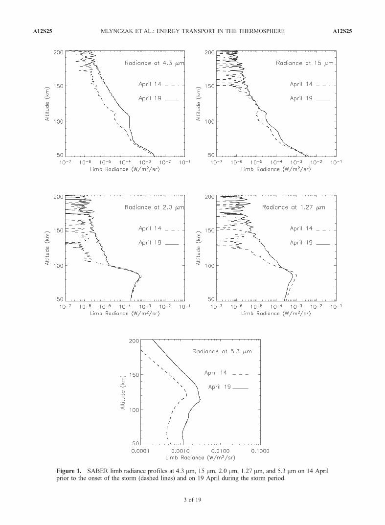
Figure 1. SABER limb radiance profiles at 4.3 mm, 15 mm, 2.0 mm, 1.27 mm, and 5.3 mm on 14 Aprilprior to the onset of the storm (dashed lines) and on 19 April during the storm period.


3 of 19

A12S25

be complemented by model analyses of emission fromatomic oxygen and of energy loss due to heat conduction.We now discuss briefly the ASPEN general circulationmodel and then continue with a detailed analysis of theSABER observations of the NO and CO2 emissions.

2.2. ASPEN Model

[9] The model used here is the National Center forAtmospheric Research (NCAR) Thermosphere IonosphereMesosphere Electrodynamics General Circulation Model(TIME-GCM), which has been ported to the SouthwestResearch Institute in San Antonio, Texas where it runs on aBeowulf computer system [Crowley et al., 1999] and isknown as the ASPEN model. The TIME-GCM was de-scribed by Roble and Ridley [1994] and is the latest in aseries of three-dimensional (3-D) models developed atNCAR. The ASPEN model is commensurate with thecurrent version of the TIME-GCM in most respects. Theinputs required by the model include the solar flux at 57 keywavelengths, auroral particle precipitation, high-latitudeelectric fields, and tides propagating up from below the10 hPa (10 mb) lower boundary. There are many ways tospecify these inputs to the model. For simplicity, with thediurnally reproducible runs presented here, the inputs to themodel include solar flux parameterized using a fixed F10.7

index of 75, which represents typical solar minimum con-ditions. The storm-time model runs are described in detailby G. Crowley et al. (Space weather effects of the April 16–23, 2002, magnetic storm, manuscript in preparation forJournal of Geophysical Research, 2005a). Briefly, the sizeof the auroral oval and the particle characteristics are drivenby the Roble and Ridley [1987] model, using HemisphericPower measured approximately every 45 min by the NOAAsatellites. The high-latitude electric field distribution isrepresented using the Heelis et al. [1982] model with IMFBY measured by the ACE satellite and cross-cap potentialestimated from the Weimer [1996] empirical model drivenby solar wind inputs. The upward propagating tides areforced at the lower boundary of the model using seasonaltidal amplitudes and phases derived from the Global ScaleWave Model (GSWM) of Hagan et al. [1999]. The model isalso forced by gravity waves propagating from below. Thisversion of the model uses the same gravity wave dragformulation and latitude dependence as the Garcia-Solomon2-D model [Garcia et al., 1992; Garcia and Solomon,1994]. The gravity waves add directly to the energy budgetand the momentum budget and also indirectly via the eddydiffusion terms. The TIME-GCM has been described indetail by Roble [1995]. The energy equation solved by themodel and the individual energy terms are discussed byG. Crowley et al. (A theoretical study of the energeticsof the mesosphere and thermosphere: 1. Solar minimumconditions, manuscript in preparation for Journal ofGeophysical Research, 2005b).

3. Analysis of SABER Observations

[10] We conduct analysis of the SABER observations thatwill lead from the measured SABER limb radiance withinthe spectral bandpass of the instrument at 5.3 mm to anestimate of the total energy emitted by nitric oxide duringthe storm period. There are several steps in this process which

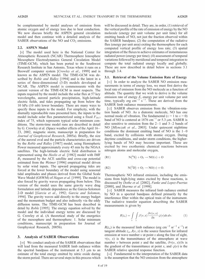
will be discussed in detail. They are, in order, (1) retrieval ofthe vertical profile of the rate of emission of energy by the NOmolecule (energy per unit volume per unit time) for allemitting bands of NO, not just the fraction observed withinthe SABER bandpass; (2) the computation of the radiativeflux (energy per unit area) exiting the thermosphere for eachcomputed vertical profile of energy loss rate; (3) spatialintegration of the fluxes to achieve estimates of instantaneousradiated power (energy per time); (4) assessment of temporalvariations followed bymeridional and temporal integration tocompute the total radiated energy locally and globally.These are now described in detail below in sections 3.1through 3.4.

3.1. Retrieval of the Volume Emission Rate of Energy

[11] In order to analyze the SABER NO emission mea-surements in terms of energy loss, we must first derive thelocal rate of emission from the NO molecule as a function ofaltitude. The quantity that we wish to derive is the volumeemission rate of energy E, energy per unit volume per unittime, typically erg cm�3 s�1. These are derived from theSABER limb radiance measurements.[12] SABER observes emission from the vibration-rota-

tion bands of NO. As a diatomic molecule, NO has onenormal mode of vibration. The fundamental (u = 1 to u = 0)band of NO is centered at 1876 cm�1 or 5.3 mm. SABER isalso sensitive to emission from the 2–1 and 3–2 bands ofNO [Mlynczak et al., 2003]. Under quiescent nighttimeconditions the dominant emitting band of NO is the 1–0band, excited by collisions with atomic oxygen. Duringdaytime conditions, and under storm conditions, the higher-lying bands of NO may become important. These areexcited by two exothermic chemical reactions betweennitrogen atoms and molecular oxygen,

N 4S� �

þ O2 ! NO uð Þ þ OðR1Þ

N 2D� �

þ O2 ! NO uð Þ þ O:ðR2Þ

Thermospheric NO infrared emission, including the emis-sions from high-lying states excited by these reactions, isdiscussed by Dothe et al. [2002], Funke and Lopez-Puertas[2000], and Sharma et al. [1998].[13] SABER measures the infrared limb radiance emitted

by NO in a spectral bandpass defined primarily by theinterference filter within the optical train of the instrument.The radiative transfer equation describing the SABERmeasurements is given by

R zoð Þ ¼Zn

Zx

J n; xð Þ @t n; xð Þ@x

j nð Þdx dn: ð1Þ

R(zo) is the measured limb radiance (erg cm�2 sr�1 s�1) attangent altitude zo, J(n, x) is the source function for infraredemission at wave number n at point x along the line of sight,t(n, x) is the transmittance of the atmosphere at wavenumber n between point x and the satellite, @t(n, x)/@x isthe gradient of the transmittance at point x, and j(n) is theSABER relative spectral response function.[14] Fundamental to the interpretation of the SABER data

is the assumption that the NO emission from the atmosphere


4 of 19

A12S25

and observed by SABER is in the weak-line limit ofradiative transfer. In the weak line limit, absorption byNO (i.e., self-absorption) is minimal along the line of sight.In this limit, all radiation emitted by the atmosphere in thedirection of the instrument escapes the atmosphere and isdetected. The radiative transfer equation in the weak linelimit is written as

R zoð Þ ¼ hc

4p

Xmj¼1

Xki¼1

Vij ni ji dxj: ð2Þ

Vij is the photon volume emission rate (photons cm�3 s�1)for ith spectral line in the jth layer of atmosphere along theline of sight, h is Planck’s constant, ni is the central wavenumber of the ith line, and c is the speed of light. Thesummations are taken over all spectral lines of NO (totalnumber equal to k) and over all atmospheric layers (totalnumber equal to m) along the line of sight at tangent altitudezo. In the weak line limit the emission is independent ofspectral line shape.[15] To evaluate the validity of the weak line limit of

radiative transfer in NO for the limb view of SABER, wecomputed the limb radiance for the NO fundamental bandduring storm conditions and elevated NO amounts. Theradiance was computed using equation (1) with the spectralresponse function set to 1.0 at all wave numbers. We alsocomputed the radiance with equation (1) but with thetransmittance computation in the weak line limit, i.e., tn =1 � kn*u, where kn is the absorption cross section and u isthe optical mass. The radiances agreed to better than 3%between 210 km and 100 km tangent height, the limits ofthis study. We conclude from this that the assumption ofweak line radiative transfer is valid for these analyses.[16] With the validity of the weak line limit of radiative

transfer established, we now move to invert the radiativetransfer equation to derive the volume emission rates.Equation (2) can readily be written as a matrix equationof the form Ae = r, where A is a triangular matrix containingthe path lengths dxj, e is a vector of volumetric emissionrates of energy (erg cm�3 s�1) to be determined, and r is avector of measured SABER limb radiances. This matrixequation is directly inverted by virtue of being a triangularmatrix. Upon inversion, the elements ej of vector e are givenby

ej ¼ hcXki¼1

Vijniji: ð3Þ

An individual element ej is the volume emission of NO ataltitude j which includes all i spectral lines of NO asweighted by the spectral response function j of theinstrument.[17] In order to estimate the total energy radiated by the

NO molecule, we must determine the total emission rate Ej

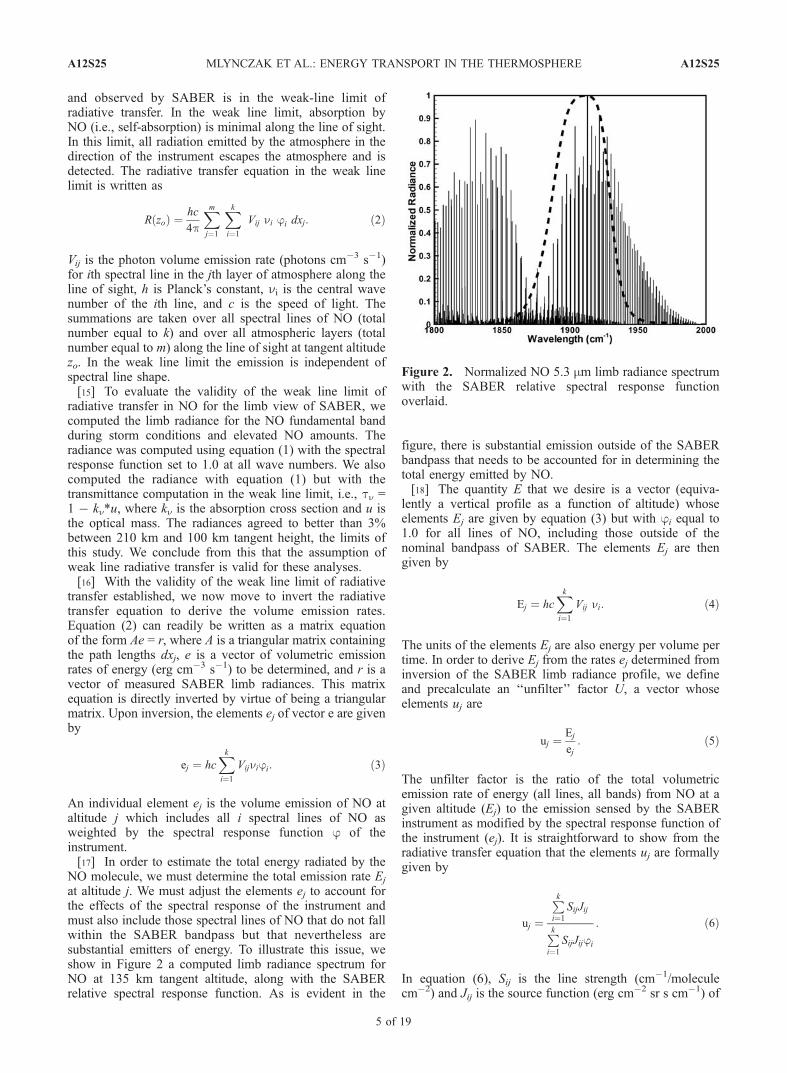
at altitude j. We must adjust the elements ej to account forthe effects of the spectral response of the instrument andmust also include those spectral lines of NO that do not fallwithin the SABER bandpass but that nevertheless aresubstantial emitters of energy. To illustrate this issue, weshow in Figure 2 a computed limb radiance spectrum forNO at 135 km tangent altitude, along with the SABERrelative spectral response function. As is evident in the

figure, there is substantial emission outside of the SABERbandpass that needs to be accounted for in determining thetotal energy emitted by NO.[18] The quantity E that we desire is a vector (equiva-

lently a vertical profile as a function of altitude) whoseelements Ej are given by equation (3) but with ji equal to1.0 for all lines of NO, including those outside of thenominal bandpass of SABER. The elements Ej are thengiven by

Ej ¼ hcXki¼1

Vij ni: ð4Þ

The units of the elements Ej are also energy per volume pertime. In order to derive Ej from the rates ej determined frominversion of the SABER limb radiance profile, we defineand precalculate an ‘‘unfilter’’ factor U, a vector whoseelements uj are

uj ¼Ej

ej: ð5Þ

The unfilter factor is the ratio of the total volumetricemission rate of energy (all lines, all bands) from NO at agiven altitude (Ej) to the emission sensed by the SABERinstrument as modified by the spectral response function ofthe instrument (ej). It is straightforward to show from theradiative transfer equation that the elements uj are formallygiven by

uj ¼

Pki¼1

SijJij

Pki¼1

SijJijji

: ð6Þ

In equation (6), Sij is the line strength (cm�1/moleculecm�2) and Jij is the source function (erg cm�2 sr s cm�1) of

Figure 2. Normalized NO 5.3 mm limb radiance spectrumwith the SABER relative spectral response functionoverlaid.


5 of 19

A12S25

the ith spectral line at conditions at altitude j. The sourcefunction is defined identically in equations (6) and (1). Thesummation is again over all lines and bands of the molecule.[19] The unfilter factor of equation (6) may be computed

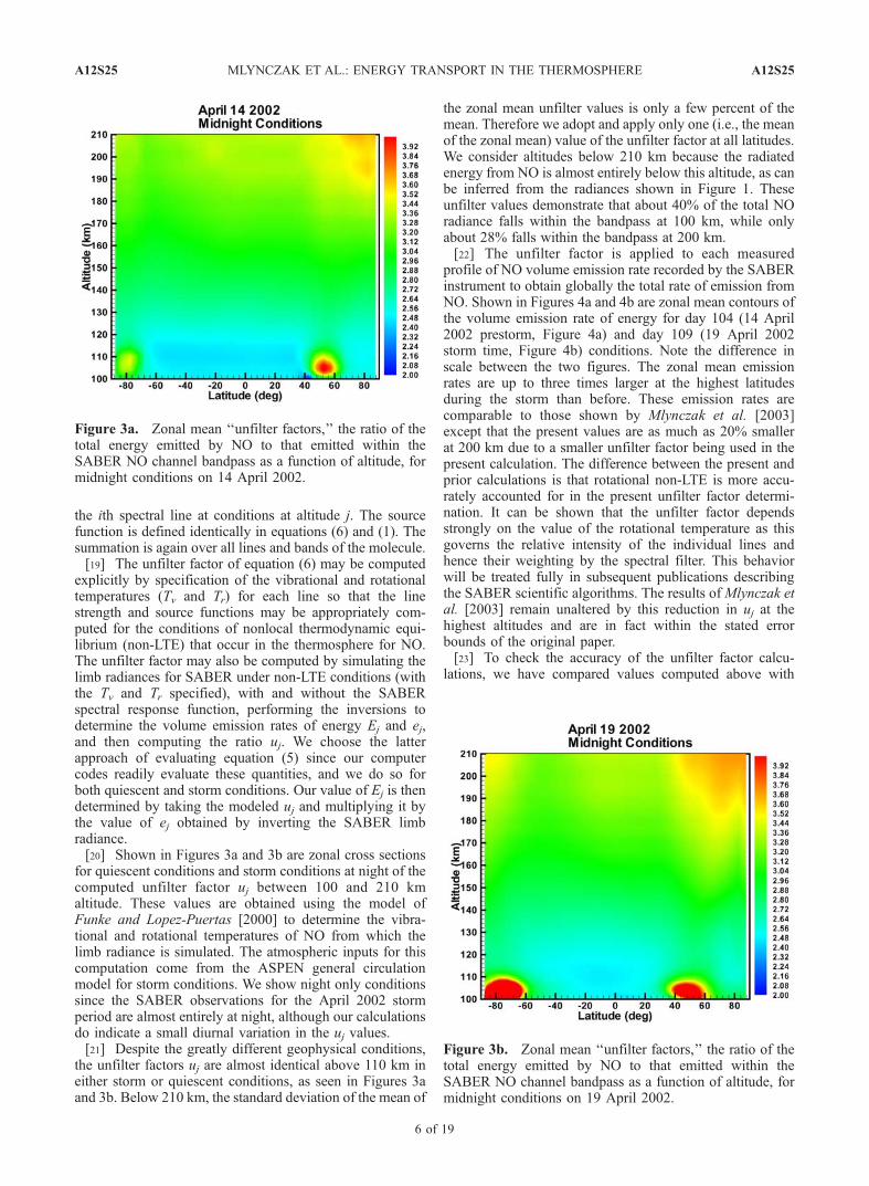
explicitly by specification of the vibrational and rotationaltemperatures (Tv and Tr) for each line so that the linestrength and source functions may be appropriately com-puted for the conditions of nonlocal thermodynamic equi-librium (non-LTE) that occur in the thermosphere for NO.The unfilter factor may also be computed by simulating thelimb radiances for SABER under non-LTE conditions (withthe Tv and Tr specified), with and without the SABERspectral response function, performing the inversions todetermine the volume emission rates of energy Ej and ej,and then computing the ratio uj. We choose the latterapproach of evaluating equation (5) since our computercodes readily evaluate these quantities, and we do so forboth quiescent and storm conditions. Our value of Ej is thendetermined by taking the modeled uj and multiplying it bythe value of ej obtained by inverting the SABER limbradiance.[20] Shown in Figures 3a and 3b are zonal cross sections

for quiescent conditions and storm conditions at night of thecomputed unfilter factor uj between 100 and 210 kmaltitude. These values are obtained using the model ofFunke and Lopez-Puertas [2000] to determine the vibra-tional and rotational temperatures of NO from which thelimb radiance is simulated. The atmospheric inputs for thiscomputation come from the ASPEN general circulationmodel for storm conditions. We show night only conditionssince the SABER observations for the April 2002 stormperiod are almost entirely at night, although our calculationsdo indicate a small diurnal variation in the uj values.[21] Despite the greatly different geophysical conditions,

the unfilter factors uj are almost identical above 110 km ineither storm or quiescent conditions, as seen in Figures 3aand 3b. Below 210 km, the standard deviation of the mean of

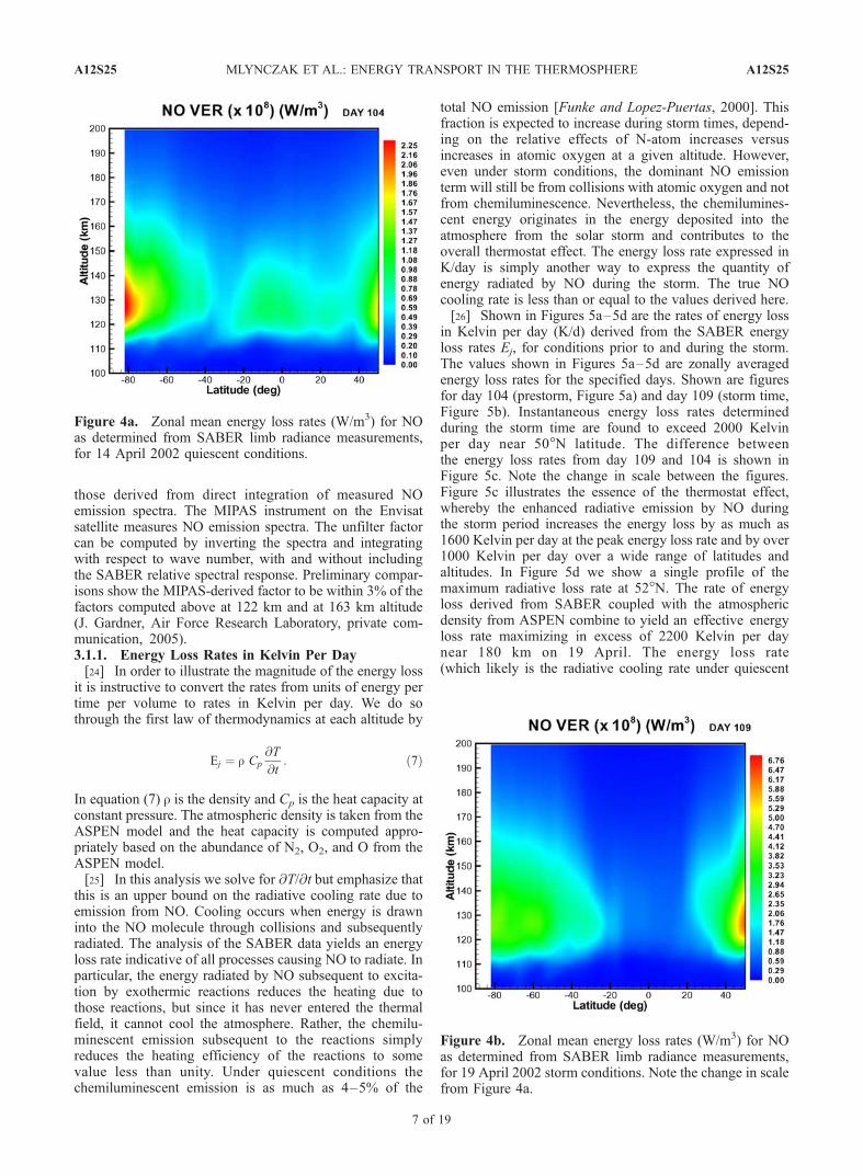
the zonal mean unfilter values is only a few percent of themean. Therefore we adopt and apply only one (i.e., the meanof the zonal mean) value of the unfilter factor at all latitudes.We consider altitudes below 210 km because the radiatedenergy from NO is almost entirely below this altitude, as canbe inferred from the radiances shown in Figure 1. Theseunfilter values demonstrate that about 40% of the total NOradiance falls within the bandpass at 100 km, while onlyabout 28% falls within the bandpass at 200 km.[22] The unfilter factor is applied to each measured

profile of NO volume emission rate recorded by the SABERinstrument to obtain globally the total rate of emission fromNO. Shown in Figures 4a and 4b are zonal mean contours ofthe volume emission rate of energy for day 104 (14 April2002 prestorm, Figure 4a) and day 109 (19 April 2002storm time, Figure 4b) conditions. Note the difference inscale between the two figures. The zonal mean emissionrates are up to three times larger at the highest latitudesduring the storm than before. These emission rates arecomparable to those shown by Mlynczak et al. [2003]except that the present values are as much as 20% smallerat 200 km due to a smaller unfilter factor being used in thepresent calculation. The difference between the present andprior calculations is that rotational non-LTE is more accu-rately accounted for in the present unfilter factor determi-nation. It can be shown that the unfilter factor dependsstrongly on the value of the rotational temperature as thisgoverns the relative intensity of the individual lines andhence their weighting by the spectral filter. This behaviorwill be treated fully in subsequent publications describingthe SABER scientific algorithms. The results of Mlynczak etal. [2003] remain unaltered by this reduction in uj at thehighest altitudes and are in fact within the stated errorbounds of the original paper.[23] To check the accuracy of the unfilter factor calcu-

lations, we have compared values computed above with

Figure 3a. Zonal mean ‘‘unfilter factors,’’ the ratio of thetotal energy emitted by NO to that emitted within theSABER NO channel bandpass as a function of altitude, formidnight conditions on 14 April 2002.

Figure 3b. Zonal mean ‘‘unfilter factors,’’ the ratio of thetotal energy emitted by NO to that emitted within theSABER NO channel bandpass as a function of altitude, formidnight conditions on 19 April 2002.


6 of 19

A12S25

those derived from direct integration of measured NOemission spectra. The MIPAS instrument on the Envisatsatellite measures NO emission spectra. The unfilter factorcan be computed by inverting the spectra and integratingwith respect to wave number, with and without includingthe SABER relative spectral response. Preliminary compar-isons show the MIPAS-derived factor to be within 3% of thefactors computed above at 122 km and at 163 km altitude(J. Gardner, Air Force Research Laboratory, private com-munication, 2005).3.1.1. Energy Loss Rates in Kelvin Per Day[24] In order to illustrate the magnitude of the energy loss

it is instructive to convert the rates from units of energy pertime per volume to rates in Kelvin per day. We do sothrough the first law of thermodynamics at each altitude by

Ej ¼ r Cp

@T

@t: ð7Þ

In equation (7) r is the density and Cp is the heat capacity atconstant pressure. The atmospheric density is taken from theASPEN model and the heat capacity is computed appro-priately based on the abundance of N2, O2, and O from theASPEN model.[25] In this analysis we solve for @T/@t but emphasize that

this is an upper bound on the radiative cooling rate due toemission from NO. Cooling occurs when energy is drawninto the NO molecule through collisions and subsequentlyradiated. The analysis of the SABER data yields an energyloss rate indicative of all processes causing NO to radiate. Inparticular, the energy radiated by NO subsequent to excita-tion by exothermic reactions reduces the heating due tothose reactions, but since it has never entered the thermalfield, it cannot cool the atmosphere. Rather, the chemilu-minescent emission subsequent to the reactions simplyreduces the heating efficiency of the reactions to somevalue less than unity. Under quiescent conditions thechemiluminescent emission is as much as 4–5% of the

total NO emission [Funke and Lopez-Puertas, 2000]. Thisfraction is expected to increase during storm times, depend-ing on the relative effects of N-atom increases versusincreases in atomic oxygen at a given altitude. However,even under storm conditions, the dominant NO emissionterm will still be from collisions with atomic oxygen and notfrom chemiluminescence. Nevertheless, the chemilumines-cent energy originates in the energy deposited into theatmosphere from the solar storm and contributes to theoverall thermostat effect. The energy loss rate expressed inK/day is simply another way to express the quantity ofenergy radiated by NO during the storm. The true NOcooling rate is less than or equal to the values derived here.[26] Shown in Figures 5a–5d are the rates of energy loss

in Kelvin per day (K/d) derived from the SABER energyloss rates Ej, for conditions prior to and during the storm.The values shown in Figures 5a–5d are zonally averagedenergy loss rates for the specified days. Shown are figuresfor day 104 (prestorm, Figure 5a) and day 109 (storm time,Figure 5b). Instantaneous energy loss rates determinedduring the storm time are found to exceed 2000 Kelvinper day near 50�N latitude. The difference betweenthe energy loss rates from day 109 and 104 is shown inFigure 5c. Note the change in scale between the figures.Figure 5c illustrates the essence of the thermostat effect,whereby the enhanced radiative emission by NO duringthe storm period increases the energy loss by as much as1600 Kelvin per day at the peak energy loss rate and by over1000 Kelvin per day over a wide range of latitudes andaltitudes. In Figure 5d we show a single profile of themaximum radiative loss rate at 52�N. The rate of energyloss derived from SABER coupled with the atmosphericdensity from ASPEN combine to yield an effective energyloss rate maximizing in excess of 2200 Kelvin per daynear 180 km on 19 April. The energy loss rate(which likely is the radiative cooling rate under quiescent

Figure 4a. Zonal mean energy loss rates (W/m3) for NOas determined from SABER limb radiance measurements,for 14 April 2002 quiescent conditions.

Figure 4b. Zonal mean energy loss rates (W/m3) for NOas determined from SABER limb radiance measurements,for 19 April 2002 storm conditions. Note the change in scalefrom Figure 4a.


7 of 19

A12S25

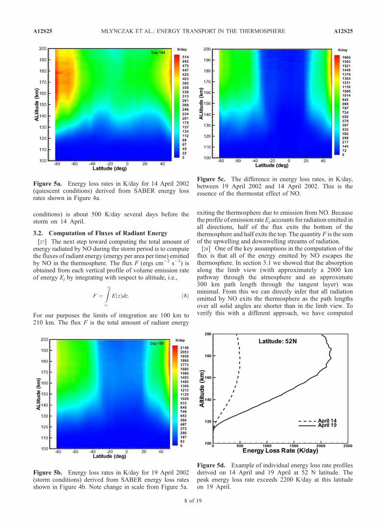
conditions) is about 500 K/day several days before thestorm on 14 April.

3.2. Computation of Fluxes of Radiant Energy

[27] The next step toward computing the total amount ofenergy radiated by NO during the storm period is to computethe fluxes of radiant energy (energy per area per time) emittedby NO in the thermosphere. The flux F (ergs cm�2 s�1) isobtained from each vertical profile of volume emission rateof energy Ej by integrating with respect to altitude, i.e.,

F ¼Zz2

z1

E zð Þdz: ð8Þ

For our purposes the limits of integration are 100 km to210 km. The flux F is the total amount of radiant energy

exiting the thermosphere due to emission from NO. Becausethe profile of emission rateEj accounts for radiation emitted inall directions, half of the flux exits the bottom of thethermosphere and half exits the top. The quantity F is the sumof the upwelling and downwelling streams of radiation.[28] One of the key assumptions in the computation of the

flux is that all of the energy emitted by NO escapes thethermosphere. In section 3.1 we showed that the absorptionalong the limb view (with approximately a 2000 kmpathway through the atmosphere and an approximate300 km path length through the tangent layer) wasminimal. From this we can directly infer that all radiationemitted by NO exits the thermosphere as the path lengthsover all solid angles are shorter than in the limb view. Toverify this with a different approach, we have computed

Figure 5a. Energy loss rates in K/day for 14 April 2002(quiescent conditions) derived from SABER energy lossrates shown in Figure 4a.

Figure 5b. Energy loss rates in K/day for 19 April 2002(storm conditions) derived from SABER energy loss ratesshown in Figure 4b. Note change in scale from Figure 5a.

Figure 5c. The difference in energy loss rates, in K/day,between 19 April 2002 and 14 April 2002. This is theessence of the thermostat effect of NO.

Figure 5d. Example of individual energy loss rate profilesderived on 14 April and 19 April at 52 N latitude. Thepeak energy loss rate exceeds 2200 K/day at this latitudeon 19 April.


8 of 19

A12S25

the escape function for radiation, G(z, z0), which describesthe probability of a photon emitted at altitude z arrivingat altitude z0 before being absorbed. The escape functionis given by the expression:

G z; z0ð Þ ¼ 1

S zð Þ

Zkn zð ÞE2 Dtn z; z0ð Þ½ �dn ð9Þ

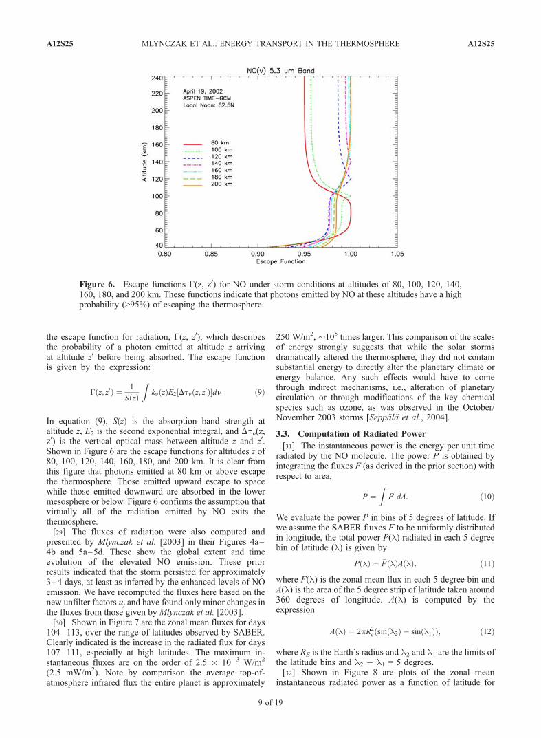
In equation (9), S(z) is the absorption band strength ataltitude z, E2 is the second exponential integral, and Dtn(z,z0) is the vertical optical mass between altitude z and z0.Shown in Figure 6 are the escape functions for altitudes z of80, 100, 120, 140, 160, 180, and 200 km. It is clear fromthis figure that photons emitted at 80 km or above escapethe thermosphere. Those emitted upward escape to spacewhile those emitted downward are absorbed in the lowermesosphere or below. Figure 6 confirms the assumption thatvirtually all of the radiation emitted by NO exits thethermosphere.[29] The fluxes of radiation were also computed and

presented by Mlynczak et al. [2003] in their Figures 4a–4b and 5a–5d. These show the global extent and timeevolution of the elevated NO emission. These priorresults indicated that the storm persisted for approximately3–4 days, at least as inferred by the enhanced levels of NOemission. We have recomputed the fluxes here based on thenew unfilter factors uj and have found only minor changes inthe fluxes from those given by Mlynczak et al. [2003].[30] Shown in Figure 7 are the zonal mean fluxes for days

104–113, over the range of latitudes observed by SABER.Clearly indicated is the increase in the radiated flux for days107–111, especially at high latitudes. The maximum in-stantaneous fluxes are on the order of 2.5 � 10�3 W/m2

(2.5 mW/m2). Note by comparison the average top-of-atmosphere infrared flux the entire planet is approximately

250 W/m2, �105 times larger. This comparison of the scalesof energy strongly suggests that while the solar stormsdramatically altered the thermosphere, they did not containsubstantial energy to directly alter the planetary climate orenergy balance. Any such effects would have to comethrough indirect mechanisms, i.e., alteration of planetarycirculation or through modifications of the key chemicalspecies such as ozone, as was observed in the October/November 2003 storms [Seppala et al., 2004].

3.3. Computation of Radiated Power

[31] The instantaneous power is the energy per unit timeradiated by the NO molecule. The power P is obtained byintegrating the fluxes F (as derived in the prior section) withrespect to area,

P ¼Z

F dA: ð10Þ

We evaluate the power P in bins of 5 degrees of latitude. Ifwe assume the SABER fluxes F to be uniformly distributedin longitude, the total power P(l) radiated in each 5 degreebin of latitude (l) is given by

P lð Þ ¼ �F lð ÞA lð Þ; ð11Þ

where F(l) is the zonal mean flux in each 5 degree bin andA(l) is the area of the 5 degree strip of latitude taken around360 degrees of longitude. A(l) is computed by theexpression

A lð Þ ¼ 2pR2e sin l2ð Þ � sin l1ð Þð Þ; ð12Þ

where RE is the Earth’s radius and l2 and l1 are the limits ofthe latitude bins and l2 � l1 = 5 degrees.[32] Shown in Figure 8 are plots of the zonal mean

instantaneous radiated power as a function of latitude for

Figure 6. Escape functions G(z, z0) for NO under storm conditions at altitudes of 80, 100, 120, 140,160, 180, and 200 km. These functions indicate that photons emitted by NO at these altitudes have a highprobability (>95%) of escaping the thermosphere.


9 of 19

A12S25

Figure 7. Zonal mean fluxes (W/m2) of energy emitted by NO in the thermosphere for days 104 (14 April2002) through day 113 (23 April 2002). Note the large increases at middle and high latitudes on days 107through 111 (17 April through 21 April) of 2002.


10 of 19

A12S25

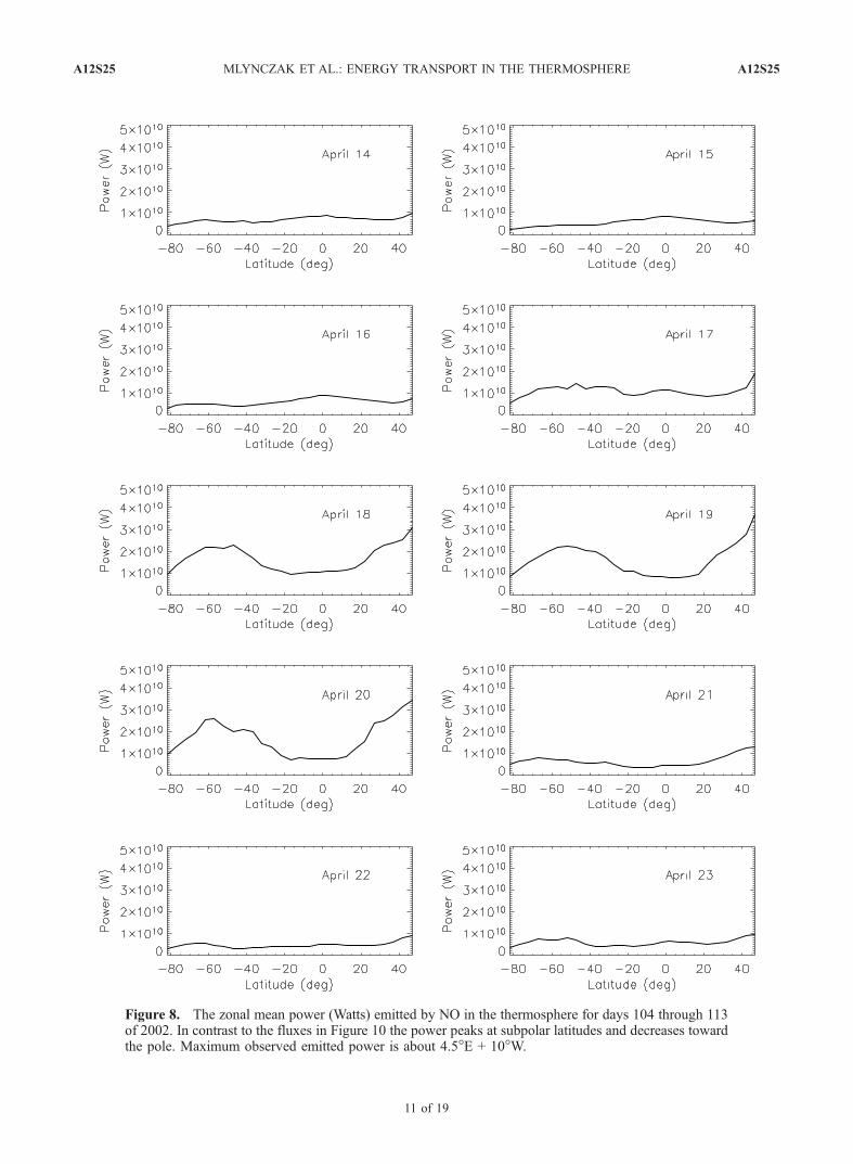
Figure 8. The zonal mean power (Watts) emitted by NO in the thermosphere for days 104 through 113of 2002. In contrast to the fluxes in Figure 10 the power peaks at subpolar latitudes and decreases towardthe pole. Maximum observed emitted power is about 4.5�E + 10�W.


11 of 19

A12S25

days 104 through 113. Note that in contrast to theradiated fluxes, the radiated power peaks at latitudesaround 50 degrees in the southern hemisphere. The lackof SABER coverage above 50 degrees north at this timeprecludes determination of the latitude at which theradiated power peaks in the northern hemisphere. How-ever, we note that by definition the radiated power mustgo to zero at the poles. The peak radiated power in thenorthern hemisphere derived here is in excess of 4 �1010 W on 19 April. The power in Figure 8 shows arather uniform distribution as a function of latitude priorto and after the storm, with peak power occurring at highlatitudes but away from the poles during the storm. Thereis a clear hemispheric asymmetry in the radiated powerduring the storm. The elevated power amounts over thebackground levels clearly indicate the effects of the stormare present on 17–20 April, with perhaps the suggestionof some high northern latitude effects on 21 April.

3.4. Computation of Radiated Energy ThroughTemporal and Meridional Integration

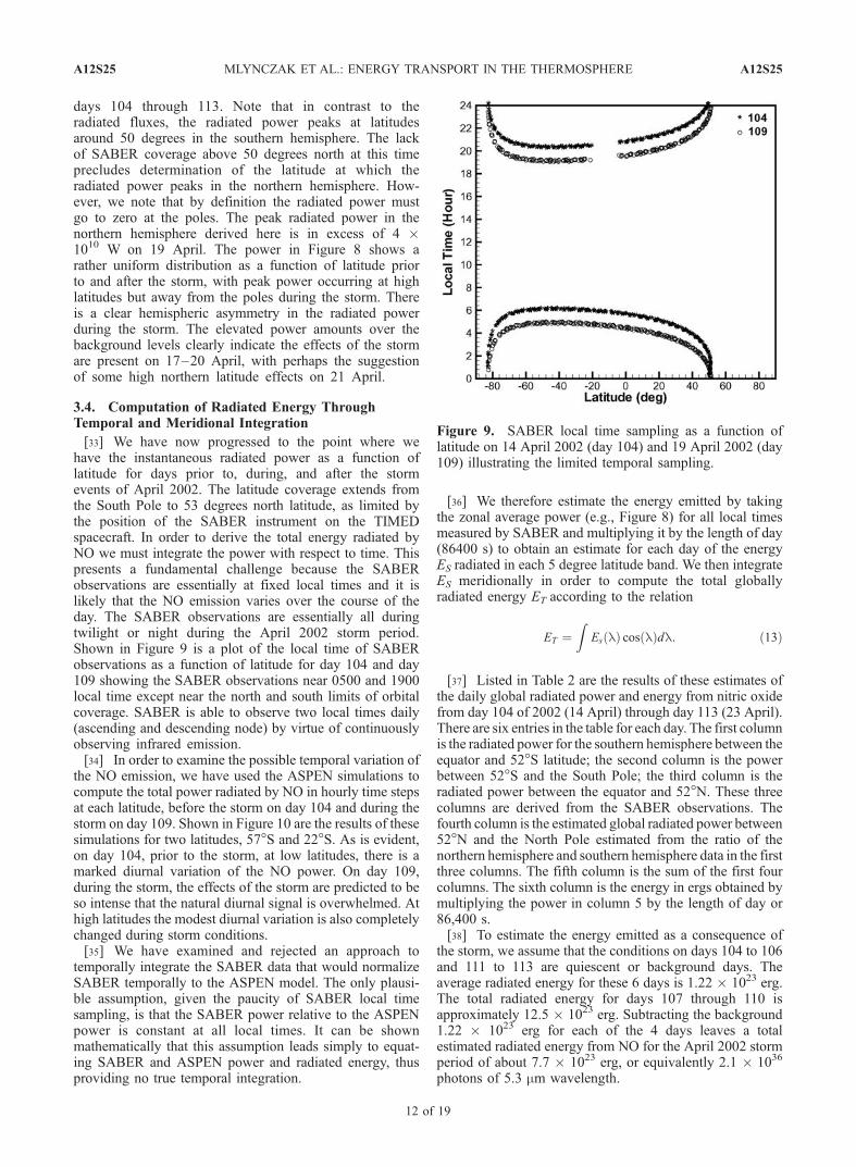
[33] We have now progressed to the point where wehave the instantaneous radiated power as a function oflatitude for days prior to, during, and after the stormevents of April 2002. The latitude coverage extends fromthe South Pole to 53 degrees north latitude, as limited bythe position of the SABER instrument on the TIMEDspacecraft. In order to derive the total energy radiated byNO we must integrate the power with respect to time. Thispresents a fundamental challenge because the SABERobservations are essentially at fixed local times and it islikely that the NO emission varies over the course of theday. The SABER observations are essentially all duringtwilight or night during the April 2002 storm period.Shown in Figure 9 is a plot of the local time of SABERobservations as a function of latitude for day 104 and day109 showing the SABER observations near 0500 and 1900local time except near the north and south limits of orbitalcoverage. SABER is able to observe two local times daily(ascending and descending node) by virtue of continuouslyobserving infrared emission.[34] In order to examine the possible temporal variation of

the NO emission, we have used the ASPEN simulations tocompute the total power radiated by NO in hourly time stepsat each latitude, before the storm on day 104 and during thestorm on day 109. Shown in Figure 10 are the results of thesesimulations for two latitudes, 57�S and 22�S. As is evident,on day 104, prior to the storm, at low latitudes, there is amarked diurnal variation of the NO power. On day 109,during the storm, the effects of the storm are predicted to beso intense that the natural diurnal signal is overwhelmed. Athigh latitudes the modest diurnal variation is also completelychanged during storm conditions.[35] We have examined and rejected an approach to

temporally integrate the SABER data that would normalizeSABER temporally to the ASPEN model. The only plausi-ble assumption, given the paucity of SABER local timesampling, is that the SABER power relative to the ASPENpower is constant at all local times. It can be shownmathematically that this assumption leads simply to equat-ing SABER and ASPEN power and radiated energy, thusproviding no true temporal integration.

[36] We therefore estimate the energy emitted by takingthe zonal average power (e.g., Figure 8) for all local timesmeasured by SABER and multiplying it by the length of day(86400 s) to obtain an estimate for each day of the energyES radiated in each 5 degree latitude band. We then integrateES meridionally in order to compute the total globallyradiated energy ET according to the relation

ET ¼Z

Es lð Þ cos lð Þdl: ð13Þ

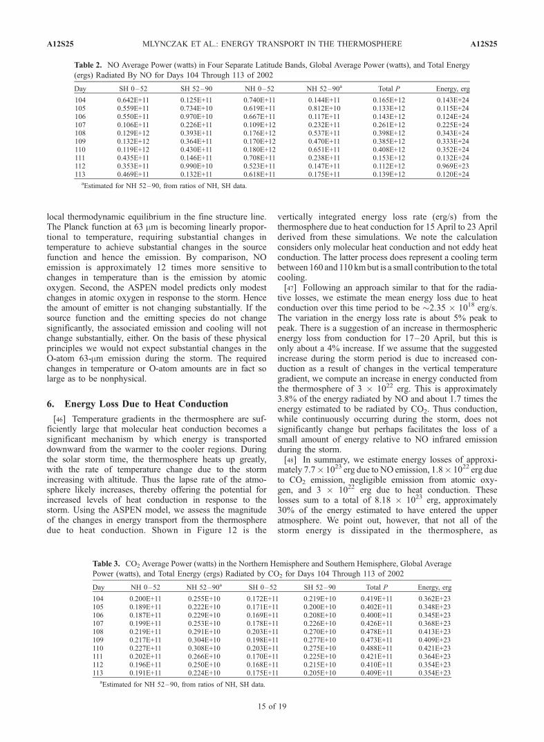
[37] Listed in Table 2 are the results of these estimates ofthe daily global radiated power and energy from nitric oxidefrom day 104 of 2002 (14 April) through day 113 (23 April).There are six entries in the table for each day. The first columnis the radiated power for the southern hemisphere between theequator and 52�S latitude; the second column is the powerbetween 52�S and the South Pole; the third column is theradiated power between the equator and 52�N. These threecolumns are derived from the SABER observations. Thefourth column is the estimated global radiated power between52�N and the North Pole estimated from the ratio of thenorthern hemisphere and southern hemisphere data in the firstthree columns. The fifth column is the sum of the first fourcolumns. The sixth column is the energy in ergs obtained bymultiplying the power in column 5 by the length of day or86,400 s.[38] To estimate the energy emitted as a consequence of

the storm, we assume that the conditions on days 104 to 106and 111 to 113 are quiescent or background days. Theaverage radiated energy for these 6 days is 1.22 � 1023 erg.The total radiated energy for days 107 through 110 isapproximately 12.5 � 1023 erg. Subtracting the background1.22 � 1023 erg for each of the 4 days leaves a totalestimated radiated energy from NO for the April 2002 stormperiod of about 7.7 � 1023 erg, or equivalently 2.1 � 1036

photons of 5.3 mm wavelength.

Figure 9. SABER local time sampling as a function oflatitude on 14 April 2002 (day 104) and 19 April 2002 (day109) illustrating the limited temporal sampling.


12 of 19

A12S25

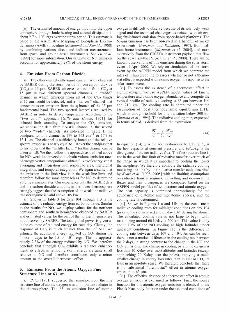
[39] The estimated amount of energy input into the upperatmosphere through Joule heating and auroral dissipation isabout 2.7 � 1024 ergs over the storm period. This estimate isbased on the Assimilative Mapping of Ionospheric Electro-dynamics (AMIE) procedure [Richmond and Kamide, 1988]by combining various direct and indirect measurementsfrom space- and ground-based instruments. See Lu et al.[1998] for more information. Our estimate of NO emissionaccounts for approximately 28% of the storm energy.

4. Emission From Carbon Dioxide

[40] The other energetically significant emission observedby SABER during the storm period is from carbon dioxide(CO2) at 15 mm. SABER observes emission from CO2 at15 mm in two different spectral channels, a ‘‘wide’’channel in which emission from all of the CO2 bandsat 15 mm would be detected, and a ‘‘narrow’’ channel thatconcentrates on emission from the q-branch of the 15 mmfundamental band. The two spectral intervals are used bySABER in order to derive temperature according to the‘‘two color’’ approach [Gille and House, 1971] forinfrared limb sounding. To analyze the CO2 emission,we choose the data from SABER channel 3, the secondof two ‘‘wide’’ channels. As indicated in Table 1, thebandpass for this channel is 579 to 763 cm�1 or 17.3 to13.1 mm. The channel is sufficiently broad and the relativespectral response is nearly equal to 1.0 over the bandpass thatto first order that the ‘‘unfilter factor’’ for this channel can betaken as 1.0. We then follow the approach as outlined abovefor NO: weak line inversion to obtain volume emission ratesof energy, vertical integration to obtain fluxes of energy, zonalaveraging and integration with respect to area, meridionalintegration, and temporal integration. We again assume thatthe emission in the limb view is in the weak line limit andtherefore follow the same approach as for NO to determinevolume emission rates. Our experience with the SABER dataand the carbon dioxide amounts in the lower thermospherestrongly suggest that the assumption of theweak line radiativetransfer regime is valid above 105 km.[41] Shown in Table 3 for days 104 through 113 is the

estimate of the radiated energy from carbon dioxide. Similarto the results for NO, we display values for the northernhemisphere and southern hemisphere observed by SABERand estimated values for the part of the northern hemispherenot observed by SABER. The total global power is given asis the estimate of radiated energy for each day. Clearly, theresponse of CO2 is much smaller than that of NO. Weestimate the additional energy radiated by CO2 during the4 storm days to be 1.8 � 1022 ergs. This is approxi-mately 2.3% of the energy radiated by NO. We thereforeconclude that although CO2 exhibits a radiance enhance-ment, its effects in removing storm energy are quite smallrelative to NO and therefore contributes only a minoramount to the overall thermostat effect.

5. Emission From the Atomic Oxygen FineStructure Line at 63 Mm

[42] Bates [1951] suggested that emission from the finestructure line of atomic oxygen was an important radiator inthe thermosphere. The 63-mm emission line of atomic

oxygen is difficult to observe because of its relatively weaksignal and the technical challenges associated with observ-ing far-infrared emission from space-based platforms. The63-mm emission has been observed in a handful of rocketexperiments [Grossman and Vollmann, 1997], from bal-loon-borne instruments [Mlynczak et al., 2004], and mostextensively from the CRISTA instrument payload that flewon the space shuttle [Grossman et al., 2000]. There are noknown observations of this emission during the solar stormevent of April 2002. We rely on simulations of the stormevent by the ASPEN model from which we compute therates of infrared cooling to assess whether or not a thermo-stat effect is expected with atomic oxygen in response to thesolar storm event.[43] To assess the existence of a thermostat effect in

atomic oxygen, we use ASPEN model values of kinetictemperature and atomic oxygen abundance and compute thevertical profile of radiative cooling at 63 mm between 100and 210 km. The cooling rate is computed under theassumption of local thermodynamic equilibrium (LTE)which is thought to hold for this transition below 300 km[Sharma et al., 1994]. The radiative cooling rate, expressedin terms of K/d, is derived from the expression

@T

@t¼ g

Cp

@Fnet

@p: ð14Þ

In equation (14), g is the acceleration due to gravity, Cp isthe heat capacity at constant pressure, and @Fnet/@p is thedivergence of the net radiative flux. The fine structure line isnot in the weak line limit of radiative transfer over much ofthe range in which it is important to cooling the lowerthermosphere. We therefore compute the radiative coolingrate using the line-by-line radiative transfer code describedby Kratz et al. [1998, 2005] with no limiting assumptionson radiative transfer regimes. Upwelling and downwellingfluxes and their divergences are computed based on theASPEN model profiles of temperature and atomic oxygen.The heat capacity is computed appropriately for theabundance of diatomic and monatomic species, and thecooling rate is determined.[44] Shown in Figures 11a and 11b are the zonal mean

radiative cooling rates for midnight conditions on day 104(prior to the storm onset) and on day 109 (during the storm).The calculated cooling rate is not large to begin with,maximizing around 60 K/day at 200 km. This value is onlyabout 10% of the NO cooling at high latitudes underquiescent conditions. In Figure 11c is the difference incooling rate between days 109 and 104. As can be seen,there is not a marked difference in the cooling rate betweenthe 2 days, in strong contrast to the change in the NO andCO2 emissions. The change in cooling by atomic oxygen isless than 10 K/day over most altitudes and latitudes (exceptapproaching 20 K/day near the poles), implying a muchsmaller change in energy loss rates than in NO or CO2, atleast in an absolute sense. We therefore conclude that thereis no substantial ‘‘thermostat’’ effect in atomic oxygenemission at 63 mm.[45] The effective absence of a thermostat effect in atomic

oxygen emission is explained as follows. First, the sourcefunction for this atomic oxygen emission is identical to thePlanck blackbody function under the assumed conditions of


13 of 19

A12S25

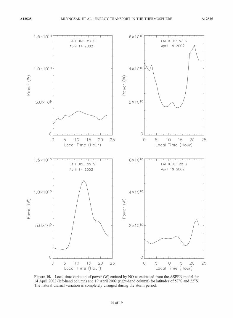
Figure 10. Local time variation of power (W) emitted by NO as estimated from the ASPEN model for14 April 2002 (left-hand column) and 19 April 2002 (right-hand column) for latitudes of 57�S and 22�S.The natural diurnal variation is completely changed during the storm period.


14 of 19

A12S25

local thermodynamic equilibrium in the fine structure line.The Planck function at 63 mm is becoming linearly propor-tional to temperature, requiring substantial changes intemperature to achieve substantial changes in the sourcefunction and hence the emission. By comparison, NOemission is approximately 12 times more sensitive tochanges in temperature than is the emission by atomicoxygen. Second, the ASPEN model predicts only modestchanges in atomic oxygen in response to the storm. Hencethe amount of emitter is not changing substantially. If thesource function and the emitting species do not changesignificantly, the associated emission and cooling will notchange substantially, either. On the basis of these physicalprinciples we would not expect substantial changes in theO-atom 63-mm emission during the storm. The requiredchanges in temperature or O-atom amounts are in fact solarge as to be nonphysical.

6. Energy Loss Due to Heat Conduction

[46] Temperature gradients in the thermosphere are suf-ficiently large that molecular heat conduction becomes asignificant mechanism by which energy is transporteddownward from the warmer to the cooler regions. Duringthe solar storm time, the thermosphere heats up greatly,with the rate of temperature change due to the stormincreasing with altitude. Thus the lapse rate of the atmo-sphere likely increases, thereby offering the potential forincreased levels of heat conduction in response to thestorm. Using the ASPEN model, we assess the magnitudeof the changes in energy transport from the thermospheredue to heat conduction. Shown in Figure 12 is the

vertically integrated energy loss rate (erg/s) from thethermosphere due to heat conduction for 15 April to 23 Aprilderived from these simulations. We note the calculationconsiders only molecular heat conduction and not eddy heatconduction. The latter process does represent a cooling termbetween 160 and 110 kmbut is a small contribution to the totalcooling.[47] Following an approach similar to that for the radia-

tive losses, we estimate the mean energy loss due to heatconduction over this time period to be �2.35 � 1018 erg/s.The variation in the energy loss rate is about 5% peak topeak. There is a suggestion of an increase in thermosphericenergy loss from conduction for 17–20 April, but this isonly about a 4% increase. If we assume that the suggestedincrease during the storm period is due to increased con-duction as a result of changes in the vertical temperaturegradient, we compute an increase in energy conducted fromthe thermosphere of 3 � 1022 erg. This is approximately3.8% of the energy radiated by NO and about 1.7 times theenergy estimated to be radiated by CO2. Thus conduction,while continuously occurring during the storm, does notsignificantly change but perhaps facilitates the loss of asmall amount of energy relative to NO infrared emissionduring the storm.[48] In summary, we estimate energy losses of approxi-

mately 7.7� 1023 erg due to NO emission, 1.8� 1022 erg dueto CO2 emission, negligible emission from atomic oxy-gen, and 3 � 1022 erg due to heat conduction. Theselosses sum to a total of 8.18 � 1023 erg, approximately30% of the energy estimated to have entered the upperatmosphere. We point out, however, that not all of thestorm energy is dissipated in the thermosphere, as

Table 2. NO Average Power (watts) in Four Separate Latitude Bands, Global Average Power (watts), and Total Energy

(ergs) Radiated By NO for Days 104 Through 113 of 2002

Day SH 0–52 SH 52–90 NH 0–52 NH 52–90a Total P Energy, erg

104 0.642E+11 0.125E+11 0.740E+11 0.144E+11 0.165E+12 0.143E+24105 0.559E+11 0.734E+10 0.619E+11 0.812E+10 0.133E+12 0.115E+24106 0.550E+11 0.970E+10 0.667E+11 0.117E+11 0.143E+12 0.124E+24107 0.106E+11 0.226E+11 0.109E+12 0.232E+11 0.261E+12 0.225E+24108 0.129E+12 0.393E+11 0.176E+12 0.537E+11 0.398E+12 0.343E+24109 0.132E+12 0.364E+11 0.170E+12 0.470E+11 0.385E+12 0.333E+24110 0.119E+12 0.430E+11 0.180E+12 0.651E+11 0.408E+12 0.352E+24111 0.435E+11 0.146E+11 0.708E+11 0.238E+11 0.153E+12 0.132E+24112 0.353E+11 0.990E+10 0.523E+11 0.147E+11 0.112E+12 0.969E+23113 0.469E+11 0.132E+11 0.618E+11 0.175E+11 0.139E+12 0.120E+24

aEstimated for NH 52–90, from ratios of NH, SH data.

Table 3. CO2 Average Power (watts) in the Northern Hemisphere and Southern Hemisphere, Global Average

Power (watts), and Total Energy (ergs) Radiated by CO2 for Days 104 Through 113 of 2002

Day NH 0–52 NH 52–90a SH 0–52 SH 52–90 Total P Energy, erg

104 0.200E+11 0.255E+10 0.172E+11 0.219E+10 0.419E+11 0.362E+23105 0.189E+11 0.222E+10 0.171E+11 0.200E+10 0.402E+11 0.348E+23106 0.187E+11 0.229E+10 0.169E+11 0.208E+10 0.400E+11 0.345E+23107 0.199E+11 0.253E+10 0.178E+11 0.226E+10 0.426E+11 0.368E+23108 0.219E+11 0.291E+10 0.203E+11 0.270E+10 0.478E+11 0.413E+23109 0.217E+11 0.304E+10 0.198E+11 0.277E+10 0.473E+11 0.409E+23110 0.227E+11 0.308E+10 0.203E+11 0.275E+10 0.488E+11 0.421E+23111 0.202E+11 0.266E+10 0.170E+11 0.225E+10 0.421E+11 0.364E+23112 0.196E+11 0.250E+10 0.168E+11 0.215E+10 0.410E+11 0.354E+23113 0.191E+11 0.224E+10 0.175E+11 0.205E+10 0.409E+11 0.354E+23

aEstimated for NH 52–90, from ratios of NH, SH data.


15 of 19

A12S25

evidenced by the observed destruction of mesosphericozone [Seppala et al., 2004].

7. Preliminary Assessment of MechanismsResponsible for NO Radiance Enhancement

[49] Now that the relative importance of the three majorinfrared radiators and heat conduction in the thermospherehas been established, a key issue is to identify themechanismsby which the NO radiation enhancement occurs. Asindicated by Mlynczak et al. [2003], there are fourmechanisms that could lead to an increase in NO emission.They are (1) increased NO abundance, (2) increased kinetic

temperature, (3) increased atomic oxygen, and (4) increasedrates of reaction leading to more chemiluminescent emission.[50] To evaluate the relative importance of these mecha-

nisms, we begin by looking in the lower thermosphere(below 140 km) at the NO concentrations recorded by theHALOE instrument on the Upper Atmosphere ResearchSatellite. Shown in Figures 13a and 13b are the ratios of thedaily zonal mean NO concentrations measured by HALOEon 20 and 21 April (during the storm) to the daily zonalmean NO concentrations measured on 9 and 10 April

Figure 11a. The radiative cooling rate (K/day) at midnightdue to emission from atomic oxygen at 63 mm on 14 April2002 prior to the storm.

Figure 11c. The difference in the radiative cooling rates ofFigures 14a and 14b, illustrating very little change incooling by atomic oxygen due to the storm.

Figure 11b. The radiative cooling rate (K/day) at midnightdue to emission from atomic oxygen at 63 mm on 19 April2002 during the storm.

Figure 12. Thermospheric cooling rate (erg/s) due to heatconduction for each day 15 April through 23 April 2002 ascomputed by the ASPEN model.


16 of 19

A12S25

(prior to the storm), in both northern (Figure 13a) andsouthern (Figure 13b) hemispheres. The HALOE datashow increases in NO by factors of 2 to 8 dependingon altitude. The HALOE data also suggest an enhance-ment in the northern hemisphere at 130 km that is afactor of 2 larger than in the southern hemisphere,consistent with the hemispheric asymmetry observed inthe SABER zonal mean fluxes and power. The HALOEdata strongly imply that changes in NO abundance are amajor factor in the observed change in NO emission inthe lower thermosphere.[51] In order to assess the importance of temperature

increases during the storm, we compute the ratio of theNO(u = 1) emission rates using ASPEN model temperaturesfrom day 104 (14 April) and 109 (19 April) assuming

everything else is constant. The ratio R we evaluate is givenby

R ¼ exp �2700=T109ð Þexp �2700=T104ð Þ ; ð15Þ

where T109 and T104 are the ASPEN temperatures on days109 and 104, respectively. The value of 2700 is the energy(in K) of the NO(1-0) fundamental transition.[52] Zonal mean values of R are shown for altitudes

between 100 and 140 km in Figure 14a and between140 km and 200 km in Figure 14b. Between 110 km and120 km, increases in temperature alone could increase theNO emission by factors of 2 to 7. Between 120 and 140 km,increases in temperature could increase the emission byfactors of 2 to 3. Above 140 km the temperature changescan increase the NO emission by as much as 50%. The effectof temperature on NO emission is the largest where thetemperature is initially the lowest. These calculations suggestthat temperature increases in the lower thermosphere cancontribute significantly to the changes in NO emission whilein the upper thermosphere the temperature changes shouldhave much less of an effect.[53] We consider now the two remaining potential mech-

anisms for NO emission enhancement, atomic oxygenincreases and chemiluminescent emission increases. Asshown above in section 5, changes in atomic oxygenpredicted by ASPEN do not appear to be large (certainlynot factors of 2 to 8 required to achieve the observed NOemission increase). Furthermore, chemiluminescent emis-sion, even during storm time, is never larger than theemission from the fundamental 1–0 band of NO. Wetherefore infer that these two mechanisms are likely notmajor factors contributing to the observed NO emissionincrease.[54] In summary, we conclude that in the lower thermo-

sphere (below 140 km) a combination of NO concentrationincreases and temperature increases likely results in the

Figure 13a. HALOE daily zonal mean NO concentrationfrom 20 April and 21 April relative to the NO measured on9 and 10 April, at the indicated latitudes in the northernhemisphere.

Figure 13b. HALOE daily zonal mean NO concentrationfrom 20 April and 21 April relative to the NO measured on9 and 10 April at the indicated latitudes in the northernhemisphere.

Figure 14a. Ratio of NO(1!0) volume emission ratecomputed with ASPEN model temperatures on 19 April(storm time) to the emission rate computed with ASPENmodel temperatures on 14 April (quiet time) to illustrate theeffect of temperature change on theNO emission rate, 100 kmto 140 km altitude.


17 of 19

A12S25

observed NO emission increase. In the middle and upperthermosphere (140 to 200 km) the observed increase in NOemission is likely due primarily to increases in NO abun-dance, with temperature increases secondary in importance.At all altitudes, changes in atomic oxygen and in chemilu-minescent emission likely play much smaller roles than theother two mechanisms.

8. Summary and Recommendations for FutureWork

[55] We have examined in detail the infrared radiativeresponse of the thermosphere during the dramatic solarstorm events of April 2002. On the basis of observationsfrom the SABER instrument on the TIMED satellite, wefind that the dominant infrared response is due to emissionfrom the nitric oxide molecule at 5.3 mm. Carbon dioxide at15 mm has a measurable but small response that is only afew percent of the nitric oxide and occurs over a muchsmaller range of altitudes. From simulations of the stormevent with the ASPEN general circulation model andconsideration of the physics of infrared radiation, we haveshown the radiative response of atomic oxygen at 63 mm tobe minimal. Computations of the rates of energy loss due tomolecular heat conduction with the ASPEN model perhapsshow a small increase in energy loss during the storm. Ratesof energy loss from nitric oxide determined from theSABER measurements exceed 2000 K/day at the peak inthe polar region near 175 km. Preliminary assessmentssuggest that enhancements in the NO emission are primarilydue to increases in the NO abundance and in temperature.The hemispheric asymmetry in observed changes in the NOabundance is consistent with the SABER observations ofenhanced radiative emission. These results confirm the‘‘natural thermostat’’ role played by nitric oxide in mitigat-ing the effects of intense solar disturbances on the atmo-

sphere. All together, the radiative and conductive lossmechanisms account for about 30% of the amount of energydeposited in the upper atmosphere.[56] This paper provides the basis for understanding the

infrared response of the thermosphere to intense solardisturbances. Nevertheless, there are still several issues thatshould be addressed. Among these are (1) a completeaccounting of the energy disposition in the mesosphere-thermosphere system relative to the estimated inputs ofthe total storm energy in the atmosphere, thereby closingthe energy budget for the storm period; (2) a refinement of therelative importance of the various mechanisms responsiblefor the NO radiance enhancements; and (3) an assessment ofpossible feedbacks in the lower atmosphere. Solving thesewill significantly enhance our understanding of the responseof the upper atmosphere and its potential coupling to the loweratmosphere to determine if these storm events alter theatmosphere for periods longer than the storm duration.

[57] Acknowledgments. MGM gratefully acknowledges the supportof the NASA Science Mission Directorate for continued support of theSABER project and the TIMED mission and also the support of the ScienceDirectorate at NASA Langley.[58] Shadia Rifai Habbal thanks Ray Roble and Timothy J. Fuller-

Rowell for their assistance in evaluating this paper.

ReferencesBates, D. R. (1951), The temperature of the upper atmosphere, Proc. Phys.Soc., Ser. B, 64, 805–821.

Crowley, G., C. Freitas, A. Ridley, D. Winningham, R. G. Roble, and A. D.Richmond (1999), Next generation space weather specification and fore-casting model, paper presented at Ionospheric Effects Symposium, Off. ofNaval Res., Alexandria, Va.

Dothe, H., J. W. Duff, R. D. Sharma, and N. B. Wheeler (2002), A model ofodd nitrogen in the aurorally dosed nighttime terrestrial thermosphere,J. Geophys. Res., 107(A7), 1071, doi:10.1029/2001JA000143.

Fink, E. H., H. Kruse, D. A. Ramsay, and M. Vervoloet (1986), An electricquadruple transition: the b1 Sg

+ - a1Dg emission system of oxygen, Can. J.Phys., 64, 242–245.

Funke, B., and M. Lopez-Puertas (2000), Nonlocal thermodynamic equili-brium vibrational, rotational, and spin state distribution of NO(u = 0, 1, 2)under quiescent atmospheric conditions, J. Geophys. Res., 105(D4),4409–4426.

Garcia, R. R., and S. Solomon (1994), A new numerical model of themiddle atmosphere: 2. Ozone and related species, J. Geophys. Res., 99,12,937–12,951.

Garcia, R. R., F. Stordal, S. Solomon, and J. Kiehl (1992), A new numericalmodel of the middle atmosphere: 1. Dynamical and transport of tropo-spheric source gases, J. Geophys. Res., 97, 12,967–12,991.

Gille, J. C., and F. House (1971), On the inversion of limb radiancemeasurements. I: temperature and thickness, J. Atmos. Sci., 28,1427–1442.

Grossman, K. U., and K. Vollmann (1997), Thermal infrared measurementsin the middle and upper atmosphere, Adv. Space Res., 19, 631–638.

Grossman, K. U., M. Kaufmann, and E. Gerstner (2000), A global mea-surement of lower thermosphere atomic oxygen densities, Geophys. Res.Lett., 27, 1387–1390.

Hagan, M. E., M. D. Burrage, J. M. Forbes, J. Hackney, W. J. Randel, andX. Zhang (1999), GSWM-98: Results for migrating solar tides, J. Geo-phys. Res., 104, 6813–6827.

Heelis, R. A., J. K. Lowell, and R. W. Spiro (1982), A model of the highlatitude ionospheric convection pattern, J. Geophys. Res., 87, 6339.

Killeen, T. L., A. G. Burns, I. Azeem, S. Cochran, and R. G. Roble (1997),A theoretical analysis of the energy budget in the lower thermosphere,J. Atmos. Sol. Terr. Phys., 59, 675–689.

Kockarts, G. (1980), Nitric oxide cooling in the terrestrial thermosphere,Geophys. Res. Lett., 7, 137–140.

Kratz, D. P., M.-D. Chou, M.-H. Yan, and C.-H. Ho (1998), Minor trace gasradiative forcing calculations using the k distribution with one-parameterscaling, J. Geophys. Res., 103, 31,647–31,656.

Kratz, D. P., M. G. Mlynczak, C. J. Mertens, H. Brindley, L. L. Gordley,F. Martin-Torres, F. M. Miskolczi, and D. D. Turner (2005), An Inter-comparison of far-infrared line-by-line radiative transfer models, J. Quant.Spectrosc. Radiat. Transfer, 90(3–4), 323–341.

Figure 14b. Ratio of NO(1!0) volume emission ratecomputed with ASPEN model temperatures on 19 April(storm time) to the emission rate computed with ASPENmodel temperatures on 14 April (quiet time) to illustrate theeffect of temperature change on theNO emission rate, 140 kmto 200 km altitude.


18 of 19

A12S25

Lu, G., et al. (1998), Global energy deposition during the January 1997magnetic cloud event, J. Geophys. Res., 103, 11,695–11,684.

Maeda, S., T. J. Fuller-Rowell, and D. S. Evans (1992), Heat budget of thethermosphere and temperature variations during the recovery phase of ageomagnetic storm, J. Geophys. Res., 97(A10), 14,947–14,957.

Mlynczak, M. G. (1995), Energetics of the middle atmosphere: Theory andobservation requirements, Adv. Space Res., 17, 117–126.

Mlynczak, M. G. (1997), Energetics of the mesosphere and lower thermo-sphere and the SABER experiment, Adv. Space Res., 20, 1177–1183.

Mlynczak, M. G., et al. (2003), The natural thermostat of nitric oxideemission at 5.3 mm in the thermosphere observed during the solar stormsof April 2002, Geophys. Res. Lett., 30(21), 2100, doi:10.1029/2003GL017693.

Mlynczak, M. G., F. J. Martin-Torres, D. G. Johnson, D. P. Kratz, W. A.Traub, and K. Jucks (2004), Observations of the O(3P) fine structure lineat 63 mm in the upper mesosphere and lower thermosphere, J. Geophys.Res., 109, A12306, doi:10.1029/2004JA010595.

Richmond, A. D., and Y. Kamide (1988), Mapping electrodynamic featuresof the high-latitude ionosphere from localized observations: Technique,J. Geophys. Res., 93, 5741–5759.

Roble, R. G. (1995), Energetics of the mesosphere and thermosphere, inTheUpperMesosphere and Lower Thermosphere: A Review of Experimentand Theory, Geophys. Monogr. Ser., vol. 87, edited by R. M. Johnson andT. L. Killeen, pp. 1–21, AGU, Washington, D. C.

Roble, R. G., and E. C. Ridley (1987), An auroral model for the NCARthermospheric general circulation model (TGCM), Ann. Geophys., 5,369.

Roble, R. G., and E. C. Ridley (1994), Thermosphere-Ionosphere-Meso-sphere-Electro Dynamics General Circulation Model (TIME-GCM):Equinox solar cycle minimum simulations (300–500 km), Geophys.Res. Lett., 22, 417.

Russell, J. M., M. G. Mlynczak, L. L. Gordley, J. Tansock, and R. Esplin(1999), An overview of the SABER experiment and preliminary calibra-tion results, in Proceedings of the 44th Annual Meeting, Denver, Color-ado, July 18–23, vol. 3756, pp. 277–288, SPIE, Bellingham, Wash.

Seppala, A., P. T. Verronen, E. Kyrola, S. Hassinen, and L. Backman(2004), Solar proton events of October–November 2003: Ozone deple-

tion in the northern hemisphere polar winter as seen by GOMOS/Envisat,Geophys. Res. Lett., 31, L19107, doi:10.1029/2004GL021042.

Sharma, R. D., B. Zygelman, F. von Esse, and A. Dalgarno (1994), On therelationship between the population of the fine structure levels of theground electronic state of atomic oxygen and the translational tempera-ture, Geophys. Res. Lett., 21, 1731–1734.

Sharma, R. D., H. Dothe, and J. W. Duff (1998), Model of the 5.3 mmradiance form NO during the sunlit thermosphere, J. Geophys. Res., 103,14,753–14,758.

Weimer, D. R. (1996), A flexible IMF dependent model of high-latitudeelectric potentials having ‘‘space weather’’ applications, Geophys. Res.Lett., 23, 2549–2553.

��G. Crowley, Southwest Research Institute, 6220 Culebra Road, San

Antonio, TX 78228-0510, USA.B. Funke and M. Lopez-Puertas, Instituto de Astrofisica de Andalucia,

Apdo. 3004, E-18080 Granada, Spain.L. Gordley, G & A Technical Software, 11864 Canon Blvd., Suite 101,

Newport News, VA 23606, USA.J. Kozyra, University of Michigan, 2455 Hayward Street, Ann Arbor, MI

48109-2143, USA.D. P. Kratz, C. Mertens, and M. G. Mlynczak, Science Directorate,

NASA Langley Research Center, 21 Langley Blvd., Mail Stop 420,Hampton, VA 23681-0001, USA. ([email protected])G. Lu, National Center for Atmospheric Research, P. O. Box 3000,

Boulder, CO 80307-3000, USA.F. J. Martin-Torres, AS & M Inc., Mail Stop 420, Hampton, VA 23681,

USA.L. Paxton, Johns Hopkins University Applied Physics Laboratory, Laurel,

MD, USA.R. Picard, R. Sharma, and J. Winick, Air Force Research Laboratory, 29

Randolph Road, Hanscom Air Force Base, MA 01731-3010, USA.J. M. Russell III, Center for Atmospheric Sciences, Hampton University,

Hampton, VA 23668, USA.


19 of 19

A12S25

Energy transport in the thermosphere during the solar storms of April 2002

Documents

Transcript of Energy transport in the thermosphere during the solar storms of April 2002