- 1 -

EVALUATION OF SLUG FLOW-INDUCED FLEXURAL LOADING IN PIPELINES

USING A SURROGATE MODEL

Ibrahim A. Sultan (1)

1

Ahmed M. Reda (2)

Gareth L. Forbes (2)

(1) School of Science, Information Technology and Engineering, University of

Ballarat, Ballarat, VIC, Australia

(2) Department of Mechanical Engineering, Curtin University, WA, Perth, Australia

ABSTRACT

Slug flow induces vibration in pipelines which may, in some cases, result in fatigue failure.

This can result from dynamic stresses, induced by the deflection and bending moment in the

pipe span, growing to levels above the endurance limits of the pipeline material. As such it is

of paramount importance to understand and quantify the size of the pipeline response to slug

flow under given speed and damping conditions. This paper utilizes the results of an

optimization procedure to device a surrogate closed-form model which can be employed to

calculate the maximum values of the pipeline loadings at given values of speed and damping

parameters. The surrogate model is intended to replace the computationally costly numerical

procedure needed for the analysis.

1 Sultan, I.A., Reda, A. and Forbes, G. L., "Evaluation of Slug flow-induced flexural loading in pipelines using a surrogate model,” ” ASME Journal of Offshore Mechanics and Arctic Engineering, Vol (135), pp. 031703-1-031703-8, 2013.

- 2 -

The maximum values of the lateral deflection and bending moment, along with their locations,

have been calculated using the optimization method of Stochastic Perturbation and Successive

Approximations (SPSA). The accuracy of the proposed surrogate model will be validated

numerically and the model will be subsequently used in a numerical example to demonstrate

its applicability in industrial situations, an accompanying spreadsheet with this worked

example is also given.

Keywords: Pipeline Spanning-Slug Induced Fatigue.– track vibration – beam vibration -

surrogate model – SPSA – optimization.

INTRODUCTION

Slugging is one of the operational conditions subsea pipelines must encounter when

transporting multiphase fluids. The number of pipelines which operate in the multi-phase flow

regime is ever increasing. Slug flow which occurs across unsupported pipeline spans produces

vertical vibration, resulting in dynamic stresses; ultimately the pipeline can fail at the girth

weld location, especially in a corrosive environment. Therefore, it is crucial that pipeline

engineers identify potential fatigue damage arising from slug flow to ensure pipeline integrity

will not be compromised.

The analysis presented in this paper models the slug as a concentrated force traversing a simply

supported beam. This analysis obviously neglects the fact that the slug flow in reality is both

distributed, i.e. not simply at a concentrated point, and in fact has mass and inertia and is not

simply a point force. Both of the simplifications: neglecting the slug distribution and mass

have been shown to still allow accurate modeling under certain conditions. For instance Reda

- 3 -

and Forbes [1] demonstrated that the moving concentrated force model overestimates the

dynamic response when compared to the dynamic response of the moving distributed load.

Nevertheless, the dynamic response of the concentrated load is almost identical to that of the

dynamic response to loads distributed over less than 10% of the span length. This suggests that

the maximum normalized dynamic load factor, calculated by the proposed design equations,

presents the maximum possible value of that factor.

It was also shown by Reda et al [2] that modeling a slug as a moving point force, and not a

mass, thus neglecting the inertia of the slug will result in less than a 10% error in the resulting

deflection or bending moment for slug/beam mass ratios less than 20%.

The intention of this paper is to develop a simplified surrogate model to determine the

maximum normalized DLF of both vertical displacement and bending moment for an

unsupported pipe span. This set of equations can then be used to determine the bending stresses

required to perform the fatigue life estimates of pipelines. The given surrogate model equations

also allow easy calculation of the location of the maximum bending moment and displacement

of a span, which has been shown to not be constant for different slug flow speeds Reda et al

[3]. The proposed model can be employed at the early stages of the design when a number of

different span options are investigated. A surrogate model can also be used to quickly perform

sensitivity analyses to investigate the effects of uncertain input parameters such as slug speed,

slug length and pipe wall thickness. The model can be used for initial validation of finite

element calculations.

Sultan [4] suggests that surrogate models are used where the exact mathematical form of a

relationship, underlying a certain process, is not readily obtainable. In this case, empirical

methods are usually employed together with suitable regression techniques to work out a

- 4 -

substitution functional expression relating the various parameters controlling the process.

Surrogate models are used for a broad range of applications from simulating the effects of some

engine parameters on its performance Bates et al [5] to describing machining errors in turning

processes Gilsinn et al [6]. The process of obtaining a fitted model is essentially an

optimization exercise, where the difference between the estimated system output and its

measured value is to be minimized. The optimization procedure adopted in this paper is based

on the approach of Simultaneous Perturbation Stochastic Approximation (SPSA). This

approach is efficient and suited for such an intricate optimization application as abundantly

explained in literature, e.g. the excellent paper by Spall [7] and the interesting application

tackled by Kothandaraman and Rotea [8].

To obtain data sets of input parameters needed for the analysis, some researchers employ the

method of Monte Carlo simulation Jeang et al [9] or the concept of response surface Carley et

al [10] and Robinson et al [11].

The surrogate model presented in this paper could also cover a wide range of applications such

as railroad design, road bridges and many other structural situations that involve a moving load

problem. This is due to the proposed model being expressed as a function of non-dimensional

parameters relevant to these various applications. The basic concept of using a surrogate model

for the analysis of pipeline vibration has recently been presented by the authors in a conference

paper, Sultan et al [12]. However, in this current paper, the method has been expanded to also

cover the low speed range of non-dimensional speed less than 0.3.

To illustrate the application of the design equations, a worked example is included. Each step

in this example can be undertaken in early stages of design to calculate the stress range at a

pipeline girth weld. In addition an excel spreadsheet with the surrogate model equation is given

at http://espace.library.curtin.edu.au:80/R?func=dbin-jump-full&local_base=gen01-

era02&object_id=188489 for direct calculation of the dynamic response of unsupported spans.

- 5 -

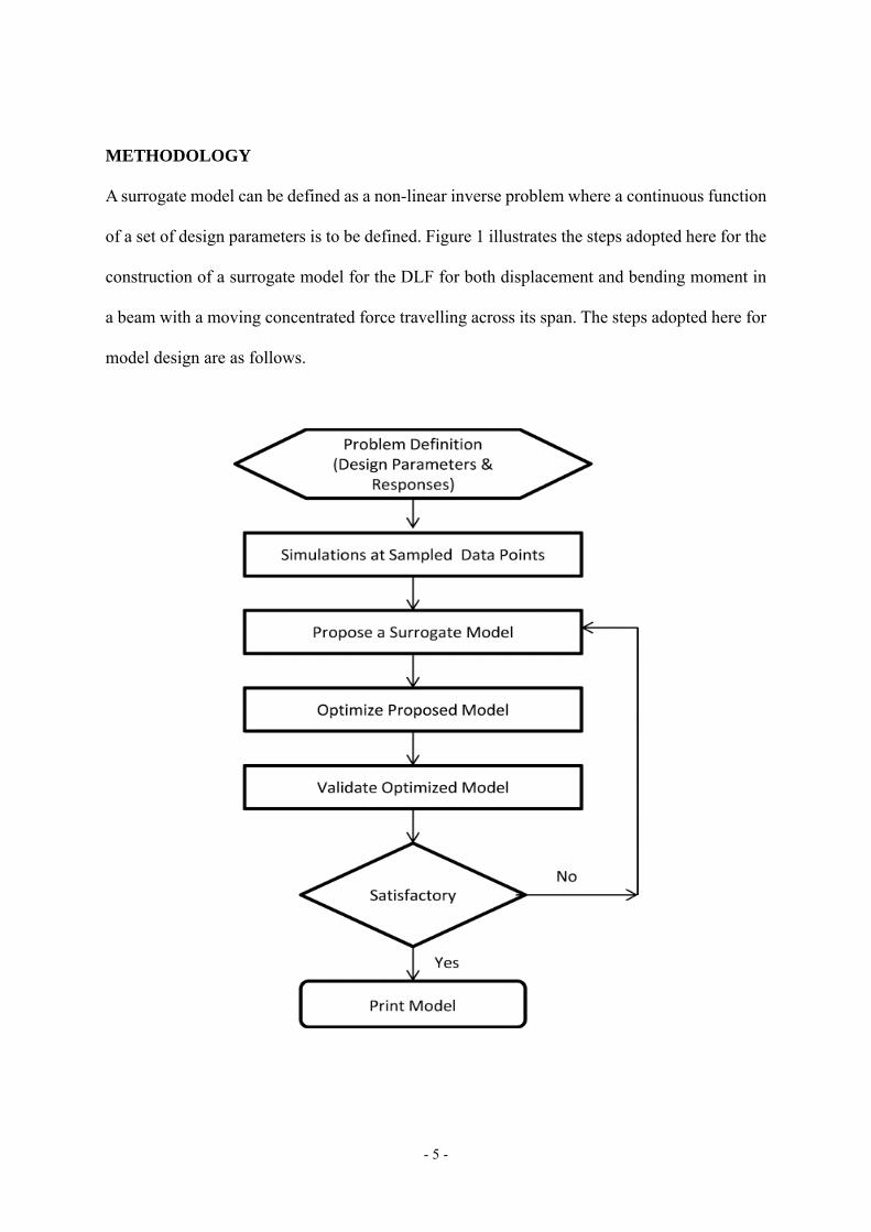
METHODOLOGY

A surrogate model can be defined as a non-linear inverse problem where a continuous function

of a set of design parameters is to be defined. Figure 1 illustrates the steps adopted here for the

construction of a surrogate model for the DLF for both displacement and bending moment in

a beam with a moving concentrated force travelling across its span. The steps adopted here for

model design are as follows.

- 6 -

Figure 1: Steps Adopted to Construct the Design Equations of DLF for

Displacement and Bending Moment

Step 1 – Data Collection: the steady state time-based Fourier expansion, presented below, for

the beam responses (both vertical deflection and bending moment) is obtained and employed

in a suitable optimization technique to find the maximum values of these response. These

maximum values will be registered for the speed parameter range of 0.03 to 1.5 and for the

damping factor range of 0.01 to 0.2. These ranges have been selected because they encompass

many practical applications encountered by design engineers.

Once the data points are generated, it is advisable to produce a set of graphs to inform the

process of proposing a mathematical formulation for the surrogate model.

Step 2 – Model Construction: guided by the graphs obtained in the first step, propose a

surrogate model.

Step 3 – Optimization: is concerned with finding the coefficients of the proposed equation

such that the surrogate model reflects the behavior of the original system as closely as possible.

This step is executed here via a suitable stochastic procedure.

Step 4 – Validation: The purpose of this step is to establish the predictive capabilities of the

surrogate model, once it is available. If the outcome from the validation process is satisfactory

then the surrogate model can be used. If not, then Steps 2 and 3 will be repeated via iterative

processes until the surrogate model is acceptable.

- 7 -

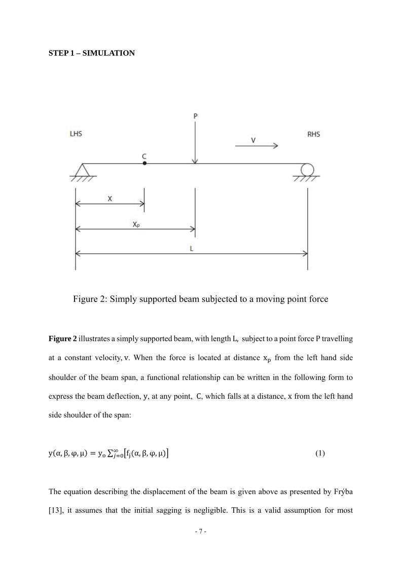
STEP 1 – SIMULATION

Figure 2: Simply supported beam subjected to a moving point force

Figure 2 illustrates a simply supported beam, with length L, subject to a point force P travelling

at a constant velocity,v. When the force is located at distance x from the left hand side

shoulder of the beam span, a functional relationship can be written in the following form to

express the beam deflection, y, at any point, C, which falls at a distance, x from the left hand

side shoulder of the span:

y α, β, φ, μ y ∑ f α, β, φ, μ (1)

The equation describing the displacement of the beam is given above as presented by Frýba

[13], it assumes that the initial sagging is negligible. This is a valid assumption for most

- 8 -

applications where the span length is less than 100 times the external diameter of the pipeline.

The parameters in the equation are defined as follows;

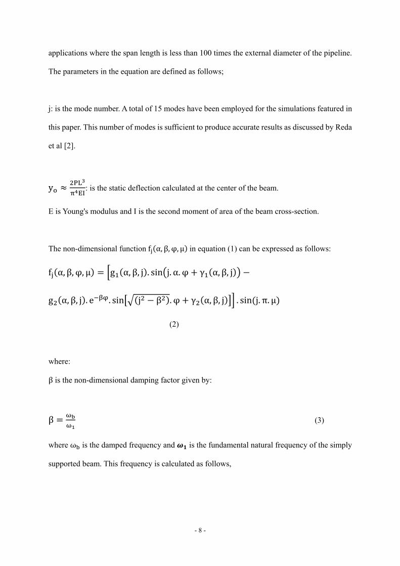
j: is the mode number. A total of 15 modes have been employed for the simulations featured in

this paper. This number of modes is sufficient to produce accurate results as discussed by Reda

et al [2].

y : is the static deflection calculated at the center of the beam.

E is Young's modulus and I is the second moment of area of the beam cross-section.

The non-dimensional function f α, β, φ, μ in equation (1) can be expressed as follows:

f α, β, φ, μ g α, β, j . sin j. α. φ γ α, β, j

g α, β, j . e . sin j β . φ γ α, β, j . sin j. π. μ

(2)

where:

β is the non-dimensional damping factor given by:

β (3)

where ω is the damped frequency and is the fundamental natural frequency of the simply

supported beam. This frequency is calculated as follows,

- 9 -

(4)

where: ρ is the mass per unit length of the beam

α is a non-dimensional speed parameter calculated by:

α (5)

ωis the circular frequency of moving load defined by:

ω (6)

φ signifies the load position, from the LHS side, and it can be calculated in accordance to the

following:

φ (7)

μdefines the x-location on the beam for the point at which the deflection calculations are being

performed. In this context μ can be defined as follows:

μ (8)

The functions included in the f expression are given as follows:

- 10 -

γ α, β, j tan (9)

γ α, β, j tan (10)

g α, β, j (11)

g α, β, j 4β (12)

The bending moment, M α, β, φ, μ , can be expressed as follows:

M α, β, φ, μ , , ,

(13)

Combining equations (1) and (13), the following expression may be written for the bending

moment:

M α, β, φ, μ ∑ j f α, β, φ, μ (14)

Equation (14) determines the bending moment at a location defined by parameter, where the

load location is defined by φ.

- 11 -

In this paper, y α, β, φ, μ and M α, β, φ, μ are replaced by their normalized dimensionless

counterparts, y α, β, φ, μ and M α, β, φ, μ , as follows;

y α, β, φ, μ y α, β, φ, μ /y (15)

and

M α, β, φ, μ M α, β, φ, μ (16)

At a given pair of α and β, an optimization technique is adopted to find the positions , and

, at which the maximum beam deflection occurs:

Maximize y α, β, φ, μ (17)

Subject to φ 0

1 μ 0

Consequently, the resulting values, and , can be used to calculate the maximum

normalized beam deflection, , which corresponds to the given values of α and β

as follows;

y α, β y α, β, φ , μ (18)

Similarly, at a given pair of α and β, an optimization technique is adopted to find the positions

of and at which the maximum beam bending moment occurs:

- 12 -

Maximize M α, β, φ, μ (19)

Subject to φ 0

1 μ 0

Consequently, the resulting values, φ and μ , can be used to calculate the maximum

normalized bending moment, M α, β which corresponds to the given values of α and β

as follows;

M α, β M α, β, φ , μ (20)

It should be pointed out here that y α, β and M α, β are referred to as the

Dynamic Load Factors (DLF) for the deflection and bending moment respectively.

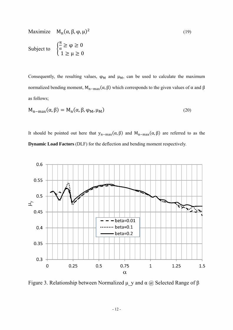
Figure 3. Relationship between Normalized μ_y and α @ Selected Range of β

- 13 -

Figure 3 describes the relationship between μ_y(point of maximum deflection along the length

of the beam) and α (non-dimensional speed of traversing force) as drawn at a selected range of

β. As can be seen from Figure 3, the maximum DLF of displacement or y_(n-max) (α,β) does

not necessarily occur at the mid-point of the beam. It can be seen that the location of the

maximum displacement alternates around the mid-point of the beam between μ_y equals to

0.55 and 0.45. The location of maximum displacement depends on both α and β.

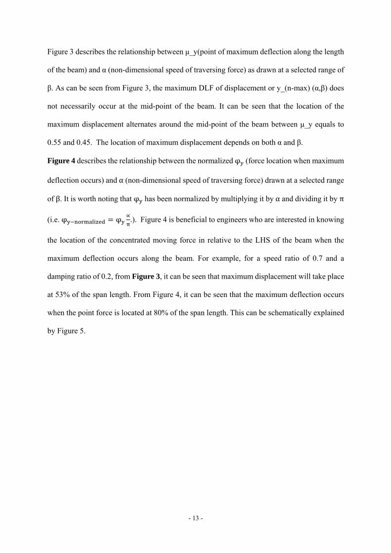
Figure 4 describes the relationship between the normalized φ (force location when maximum

deflection occurs) and α (non-dimensional speed of traversing force) drawn at a selected range

ofβ. It is worth noting that φ has been normalized by multiplying it by α and dividing it by π

(i.e. φ φ ∝.). Figure 4 is beneficial to engineers who are interested in knowing

the location of the concentrated moving force in relative to the LHS of the beam when the

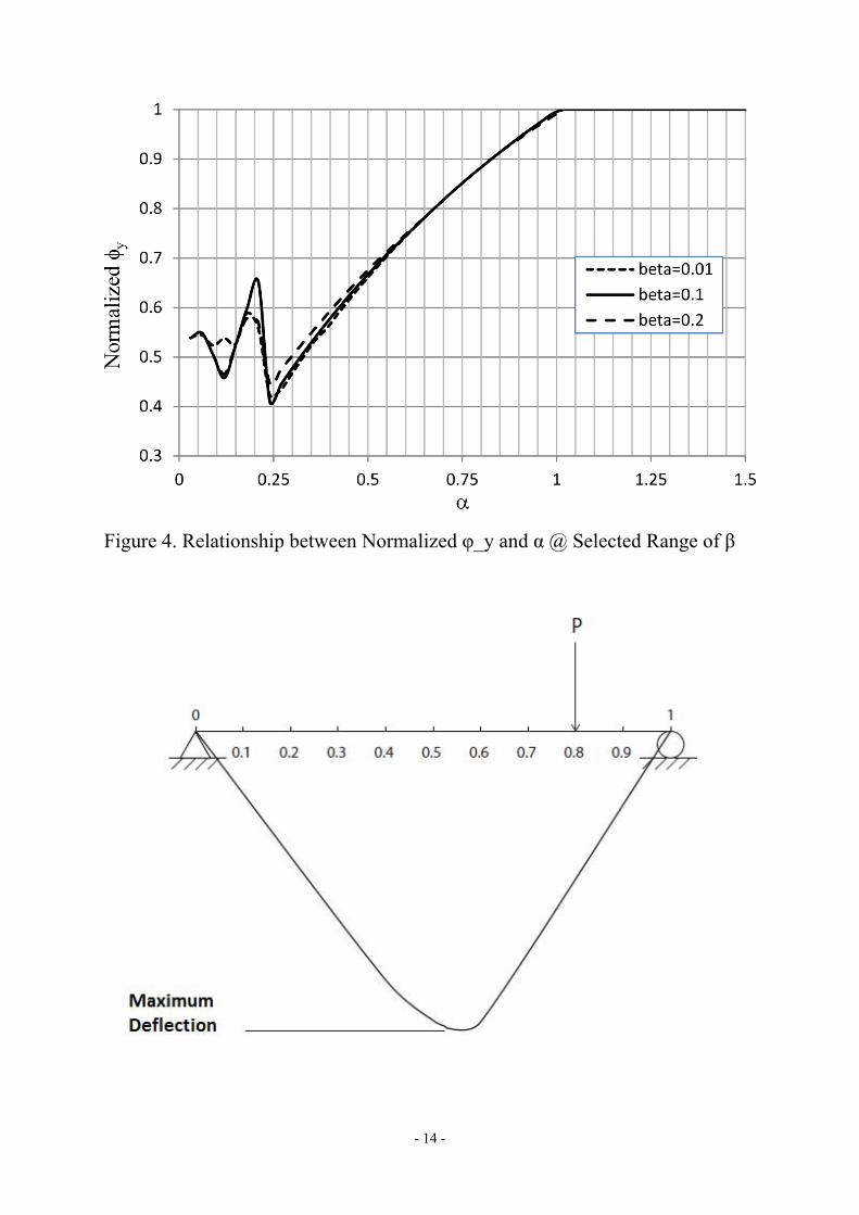
maximum deflection occurs along the beam. For example, for a speed ratio of 0.7 and a

damping ratio of 0.2, from Figure 3, it can be seen that maximum displacement will take place

at 53% of the span length. From Figure 4, it can be seen that the maximum deflection occurs

when the point force is located at 80% of the span length. This can be schematically explained

by Figure 5.

- 14 -

Figure 4. Relationship between Normalized φ_y and α @ Selected Range of β

- 15 -

Figure 5. A Schematic Diagram Showing the maximum deflection and force

location@ α = 0.7.

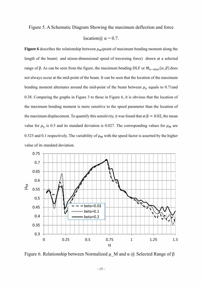
Figure 6 describes the relationship between (point of maximum bending moment along the

length of the beam) and α(non-dimensional speed of traversing force) drawn at a selected

range ofβ. As can be seen from the figure, the maximum bending DLF or , does

not always occur at the mid-point of the beam. It can be seen that the location of the maximum

bending moment alternates around the mid-point of the beam between equals to 0.71and

0.38. Comparing the graphs in Figure 3 to those in Figure 6, it is obvious that the location of

the maximum bending moment is more sensitive to the speed parameter than the location of

the maximum displacement. To quantify this sensitivity, it was found that at β 0.02, the mean

value for is 0.5 and its standard deviation is 0.027. The corresponding values for are

0.525 and 0.1 respectively. The variability of μ with the speed factor is asserted by the higher

value of its standard deviation.

Figure 6. Relationship between Normalized μ_M and α @ Selected Range of β

- 16 -

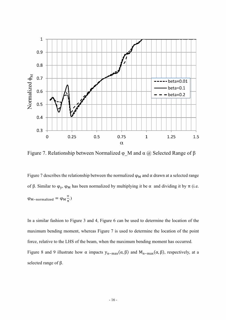
Figure 7. Relationship between Normalized φ_M and α @ Selected Range of β

Figure 7 describes the relationship between the normalized φ and α drawn at a selected range

of β. Similar to φ , φ has been normalized by multiplying it be α and dividing it by π (i.e.

φ φ ∝.)

In a similar fashion to Figure 3 and 4, Figure 6 can be used to determine the location of the

maximum bending moment, whereas Figure 7 is used to determine the location of the point

force, relative to the LHS of the beam, when the maximum bending moment has occurred.

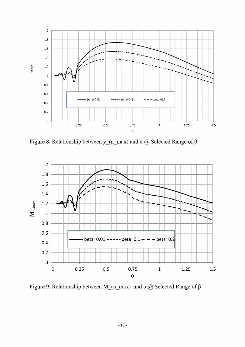
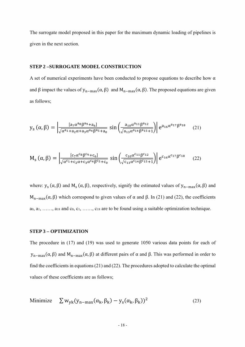
Figure 8 and 9 illustrate how α impacts y α, β and M α, β , respectively, at a

selected range of β.

- 17 -

Figure 8. Relationship between y_(n_max) and α @ Selected Range of β

Figure 9. Relationship between M_(n_max) and α @ Selected Range of β

- 18 -

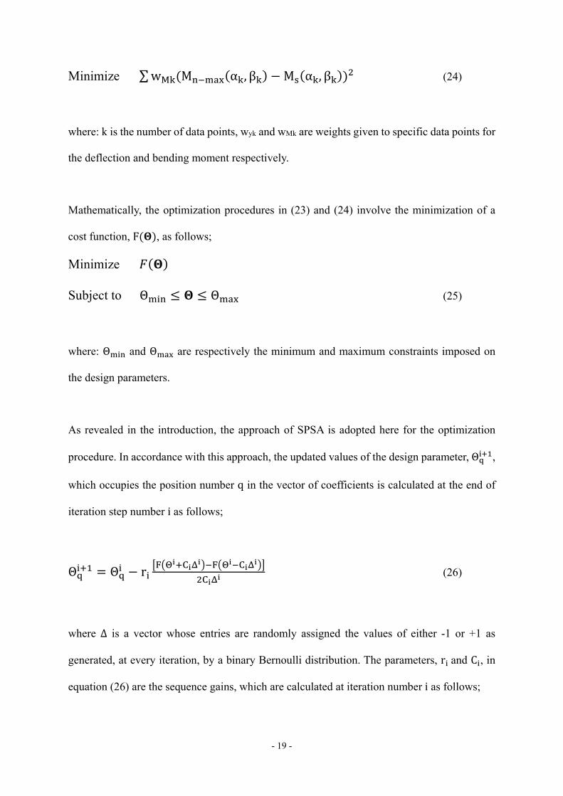
The surrogate model proposed in this paper for the maximum dynamic loading of pipelines is

given in the next section.

STEP 2 –SURROGATE MODEL CONSTRUCTION

A set of numerical experiments have been conducted to propose equations to describe how α

and β impact the values of y α, β and M α, β . The proposed equations are given

as follows;

y α, β sin e (21)

M α, β sin e (22)

where: y α, β and M α, β , respectively, signify the estimated values of y α, β and

M α, β which correspond to given values of α and β. In (21) and (22), the coefficients

a0, a1, ……, a18 and c0, c1, ……, c18 are to be found using a suitable optimization technique.

STEP 3 – OPTIMIZATION

The procedure in (17) and (19) was used to generate 1050 various data points for each of

y α, β and M α, β at different pairs of α and β. This was performed in order to

find the coefficients in equations (21) and (22). The procedures adopted to calculate the optimal

values of these coefficients are as follows;

Minimize ∑w y α , β y α , β (23)

- 19 -

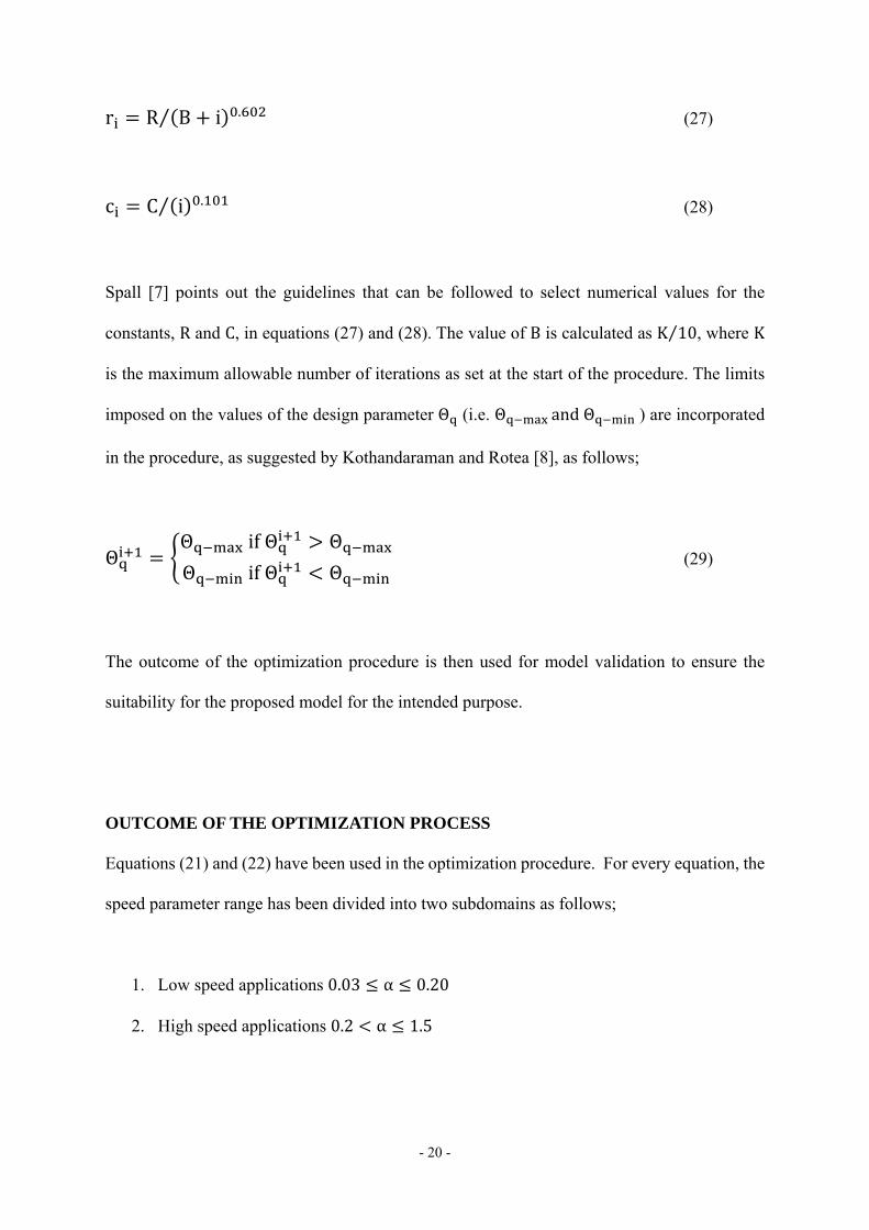
Minimize ∑w M α , β M α , β (24)

where: k is the number of data points, wyk and wMk are weights given to specific data points for

the deflection and bending moment respectively.

Mathematically, the optimization procedures in (23) and (24) involve the minimization of a

cost function, F , as follows;

Minimize

Subject to Θ Θ (25)

where: Θ and Θ are respectively the minimum and maximum constraints imposed on

the design parameters.

As revealed in the introduction, the approach of SPSA is adopted here for the optimization

procedure. In accordance with this approach, the updated values of the design parameter, Θ ,

which occupies the position number q in the vector of coefficients is calculated at the end of

iteration step number i as follows;

Θ Θ r (26)

where Δ is a vector whose entries are randomly assigned the values of either -1 or +1 as

generated, at every iteration, by a binary Bernoulli distribution. The parameters, r and C , in

equation (26) are the sequence gains, which are calculated at iteration number i as follows;

- 20 -

r R B i .⁄ (27)

c C i .⁄ (28)

Spall [7] points out the guidelines that can be followed to select numerical values for the

constants, R and C, in equations (27) and (28). The value of B is calculated as K 10⁄ , where K

is the maximum allowable number of iterations as set at the start of the procedure. The limits

imposed on the values of the design parameter Θ (i.e. Θ andΘ ) are incorporated

in the procedure, as suggested by Kothandaraman and Rotea [8], as follows;

ΘΘ ifΘ Θ

Θ ifΘ Θ (29)

The outcome of the optimization procedure is then used for model validation to ensure the

suitability for the proposed model for the intended purpose.

OUTCOME OF THE OPTIMIZATION PROCESS

Equations (21) and (22) have been used in the optimization procedure. For every equation, the

speed parameter range has been divided into two subdomains as follows;

1. Low speed applications 0.03 α 0.20

2. High speed applications 0.2 α 1.5

- 21 -

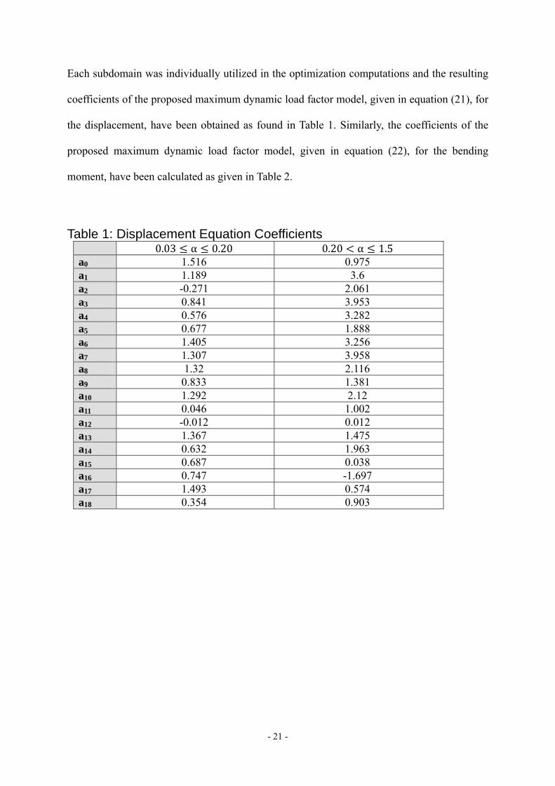
Each subdomain was individually utilized in the optimization computations and the resulting

coefficients of the proposed maximum dynamic load factor model, given in equation (21), for

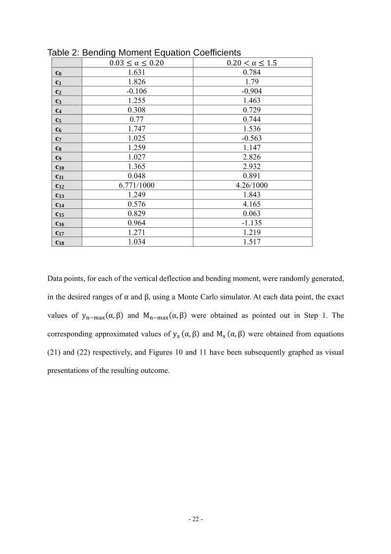
the displacement, have been obtained as found in Table 1. Similarly, the coefficients of the

proposed maximum dynamic load factor model, given in equation (22), for the bending

moment, have been calculated as given in Table 2.

Table 1: Displacement Equation Coefficients 0.03 α 0.20 0.20 α 1.5 a0 1.516 0.975 a1 1.189 3.6 a2 -0.271 2.061 a3 0.841 3.953 a4 0.576 3.282 a5 0.677 1.888 a6 1.405 3.256 a7 1.307 3.958 a8 1.32 2.116 a9 0.833 1.381 a10 1.292 2.12 a11 0.046 1.002 a12 -0.012 0.012 a13 1.367 1.475 a14 0.632 1.963 a15 0.687 0.038 a16 0.747 -1.697 a17 1.493 0.574 a18 0.354 0.903

- 22 -

Table 2: Bending Moment Equation Coefficients 0.03 α 0.20 0.20 α 1.5 c0 1.631 0.784 c1 1.826 1.79 c2 -0.106 -0.904 c3 1.255 1.463 c4 0.308 0.729 c5 0.77 0.744 c6 1.747 1.536 c7 1.025 -0.563 c8 1.259 1.147 c9 1.027 2.826 c10 1.365 2.932 c11 0.048 0.891 c12 6.771/1000 4.26/1000 c13 1.249 1.843 c14 0.576 4.165 c15 0.829 0.063 c16 0.964 -1.135 c17 1.271 1.219 c18 1.034 1.517

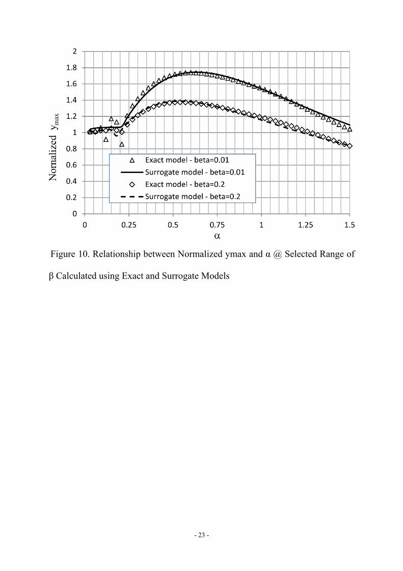
Data points, for each of the vertical deflection and bending moment, were randomly generated,

in the desired ranges of α and β, using a Monte Carlo simulator. At each data point, the exact

values of y α, β and M α, β were obtained as pointed out in Step 1. The

corresponding approximated values of y α, β and M α, β were obtained from equations

(21) and (22) respectively, and Figures 10 and 11 have been subsequently graphed as visual

presentations of the resulting outcome.

- 23 -

Figure 10. Relationship between Normalized ymax and α @ Selected Range of

β Calculated using Exact and Surrogate Models

- 24 -

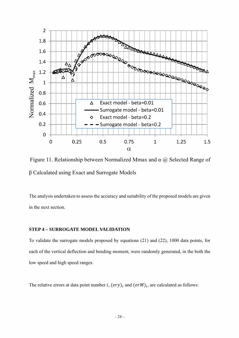
Figure 11. Relationship between Normalized Mmax and α @ Selected Range of

β Calculated using Exact and Surrogate Models

The analysis undertaken to assess the accuracy and suitability of the proposed models are given

in the next section.

STEP 4 – SURROGATE MODEL VALIDATION

To validate the surrogate models proposed by equations (21) and (22), 1000 data points, for

each of the vertical deflection and bending moment, were randomly generated, in the both the

low speed and high speed ranges.

The relative errors at data point number , and , are calculated as follows:

- 25 -

, ,

,100 (30)

, ,

,100 (31)

Low speed results

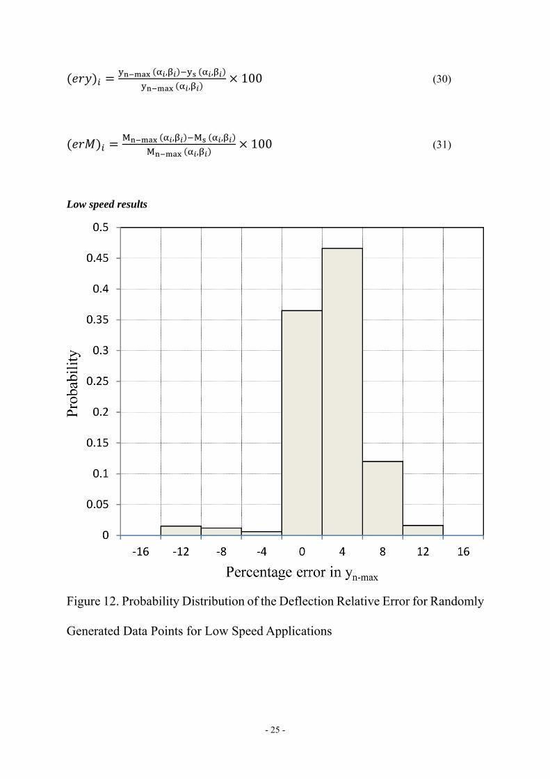
Figure 12. Probability Distribution of the Deflection Relative Error for Randomly

Generated Data Points for Low Speed Applications

- 26 -

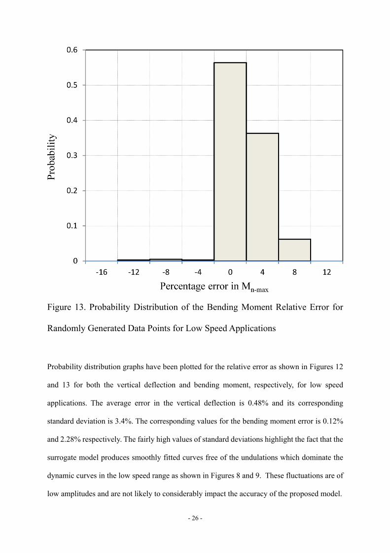
Figure 13. Probability Distribution of the Bending Moment Relative Error for

Randomly Generated Data Points for Low Speed Applications

Probability distribution graphs have been plotted for the relative error as shown in Figures 12

and 13 for both the vertical deflection and bending moment, respectively, for low speed

applications. The average error in the vertical deflection is 0.48% and its corresponding

standard deviation is 3.4%. The corresponding values for the bending moment error is 0.12%

and 2.28% respectively. The fairly high values of standard deviations highlight the fact that the

surrogate model produces smoothly fitted curves free of the undulations which dominate the

dynamic curves in the low speed range as shown in Figures 8 and 9. These fluctuations are of

low amplitudes and are not likely to considerably impact the accuracy of the proposed model.

- 27 -

For the vertical deflection, the mean value of the absolute response, y α , β , is 1.042

and the mean value of its residual error, y α , β y α , β , is 0.0063. The

corresponding values for the bending moment are 1.23 and 0.0023 respectively. The small error

values confirm the validity of the fitted low speed model and its suitability to replace the

complicated procedure, involved in solving the original model equations. This is so even

though relative error values of 12% (for either deflection or bending moment) were

registered during the calculations. Such an error level occurs with a negligible probability of

0.016 and in the low speed range which is already dominated by a number of low amplitude

fluctuations as clearly shown by Figures 8 and 9. In absolute terms a relative error value of

12% will not noticeably impact the accuracy of the surrogate model in this specific speed

range.

High speed results

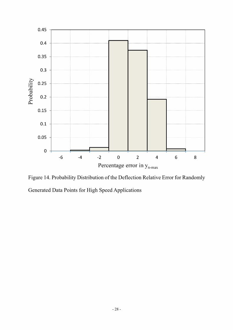
Probability distributions are plotted for the relative error as shown in Figures 14 and 15 for the

vertical deflection and bending moment, respectively, for high speed applications. The average

error in the vertical deflection is 0.54% and its corresponding standard deviation is 1.43%. The

corresponding values for the bending moment error is 0.1% and 1.15% respectively. The values

of standard deviations are relatively low to confirm the fact that the dynamic response curves

are free of fluctuations in the high speed cases as shown by Figures 8 and 9.

- 28 -

Figure 14. Probability Distribution of the Deflection Relative Error for Randomly

Generated Data Points for High Speed Applications

- 29 -

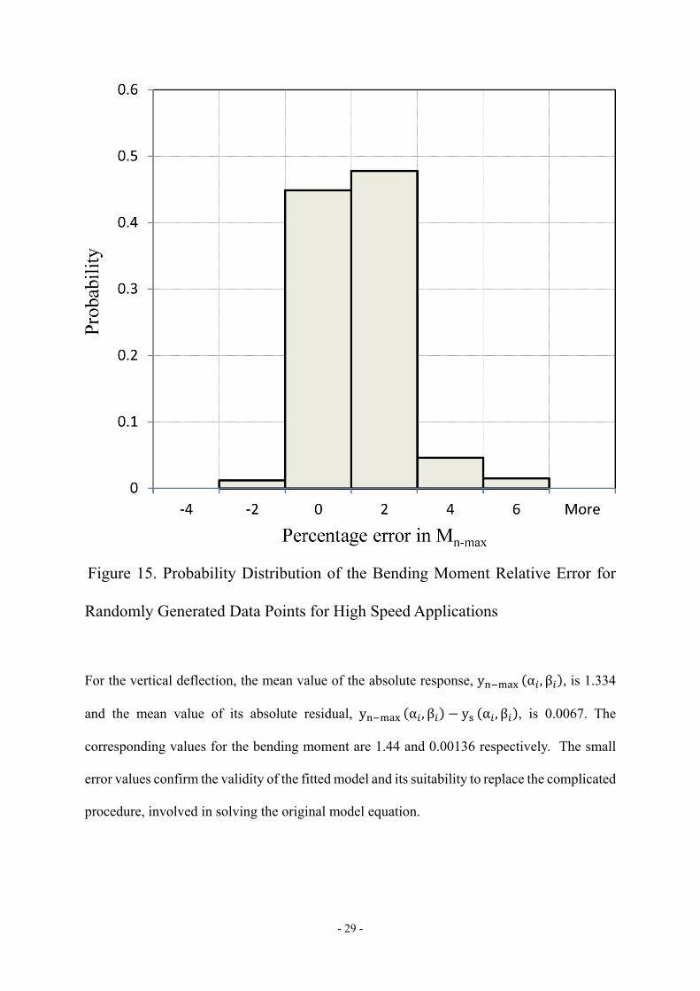
Figure 15. Probability Distribution of the Bending Moment Relative Error for

Randomly Generated Data Points for High Speed Applications

For the vertical deflection, the mean value of the absolute response, y α , β , is 1.334

and the mean value of its absolute residual, y α , β y α , β , is 0.0067. The

corresponding values for the bending moment are 1.44 and 0.00136 respectively. The small

error values confirm the validity of the fitted model and its suitability to replace the complicated

procedure, involved in solving the original model equation.

- 30 -

A numerical example is given in the next section to demonstrate the use of the proposed

surrogate model in engineering applications.

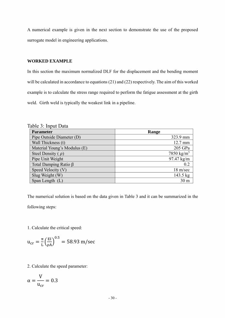
WORKED EXAMPLE

In this section the maximum normalized DLF for the displacement and the bending moment

will be calculated in accordance to equations (21) and (22) respectively. The aim of this worked

example is to calculate the stress range required to perform the fatigue assessment at the girth

weld. Girth weld is typically the weakest link in a pipeline.

Table 3: Input Data Parameter Range Pipe Outside Diameter (D) 323.9 mm Wall Thickness (t) 12.7 mm Material Young’s Modulus (E) 205 GPa Steel Density ( ) 7850 kg/m3

Pipe Unit Weight 97.47 kg/m Total Damping Ratio β 0.2 Speed Velocity (V) 18 m/sec Slug Weight (W) 143.5 kg Span Length (L) 30 m

The numerical solution is based on the data given in Table 3 and it can be summarized in the

following steps:

1. Calculate the critical speed:

u.

58.93m/sec

2. Calculate the speed parameter:

αVu

0.3

- 31 -

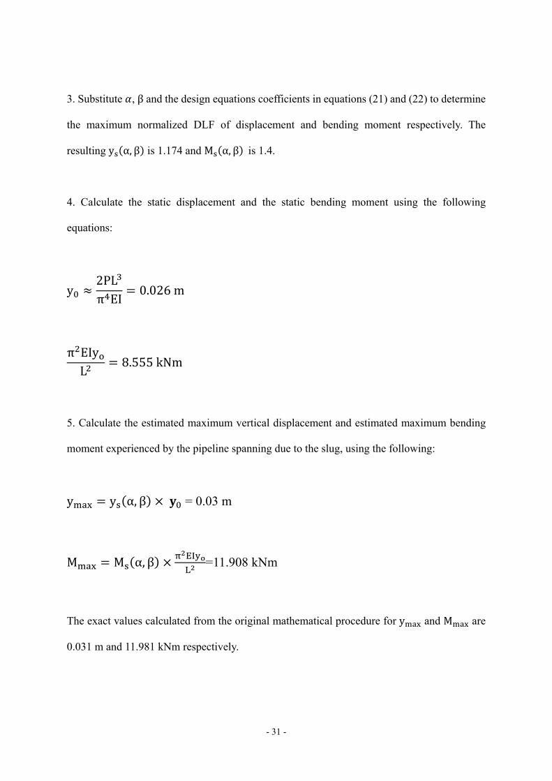
3. Substitute , β and the design equations coefficients in equations (21) and (22) to determine

the maximum normalized DLF of displacement and bending moment respectively. The

resulting y α, β is 1.174 and M α, β is 1.4.

4. Calculate the static displacement and the static bending moment using the following

equations:

y2PLπ EI

0.026m

π EIyL

8.555kNm

5. Calculate the estimated maximum vertical displacement and estimated maximum bending

moment experienced by the pipeline spanning due to the slug, using the following:

y y α, β = 0.03 m

M M α, β =11.908 kNm

The exact values calculated from the original mathematical procedure for y and M are

0.031 m and 11.981 kNm respectively.

- 32 -

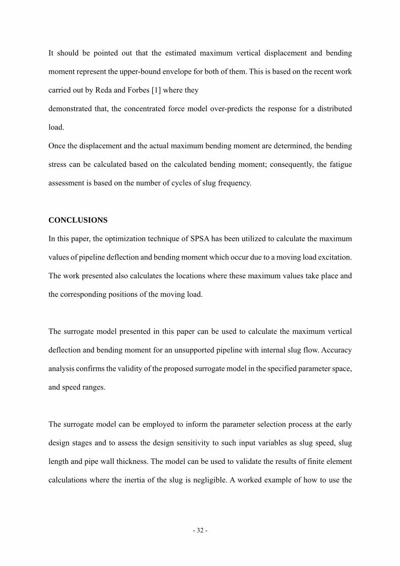
It should be pointed out that the estimated maximum vertical displacement and bending

moment represent the upper-bound envelope for both of them. This is based on the recent work

carried out by Reda and Forbes [1] where they

demonstrated that, the concentrated force model over-predicts the response for a distributed

load.

Once the displacement and the actual maximum bending moment are determined, the bending

stress can be calculated based on the calculated bending moment; consequently, the fatigue

assessment is based on the number of cycles of slug frequency.

CONCLUSIONS

In this paper, the optimization technique of SPSA has been utilized to calculate the maximum

values of pipeline deflection and bending moment which occur due to a moving load excitation.

The work presented also calculates the locations where these maximum values take place and

the corresponding positions of the moving load.

The surrogate model presented in this paper can be used to calculate the maximum vertical

deflection and bending moment for an unsupported pipeline with internal slug flow. Accuracy

analysis confirms the validity of the proposed surrogate model in the specified parameter space,

and speed ranges.

The surrogate model can be employed to inform the parameter selection process at the early

design stages and to assess the design sensitivity to such input variables as slug speed, slug

length and pipe wall thickness. The model can be used to validate the results of finite element

calculations where the inertia of the slug is negligible. A worked example of how to use the

- 33 -

surrogate model is presented in the paper and an online spreadsheet is provided for the benefit

of the reader.

Future work in this area will feature effort to replace the optimization procedure presented here,

to locate the maximum loading positions, by a simple surrogate model which will also include

the effects of axial forces and initial sagging.

REFERENCES

[1] Reda, A.M., and Forbes, G.L., 2011, “The Effect of Distribution for a Moving Force,”

in ACOUSTICS 2011, Australian Acoustical Society: Gold Coast, Queensland, Australia.

[2] Reda, A.M., Forbes, G.L. and Sultan, I.A.” Characterization of Dynamic Slug In-duced

Loads,” Proceedings of the 31st International Conference on Ocean, Offshore and Arc-tic

Engineering, Rio, Brazil, July 1-6, Paper No. OMAE 2012-83218.

[3] Reda, A.M., Forbes, G.L. and Sultan, I.A.” Characterization of Slug Flow Conditions

in Pipelines for Fatigue Analysis,” Proceedings of the 30th International Conference on Ocean,

Offshore and Arctic Engineering, Rotterdam, The Netherlands, June 19-24, Paper No. OMAE

2011-49583.

[4] Sultan, I.A., 2007, “A Surrogate Model For Interference Prevention in the Limaçon-to-

Limaçon machines”, International Journal for Computer-Aided Engineering and Software,

24(5),pp.437-449.

- 34 -

[5] Bates, R.A., Fontana, R., Randazzo, C. Vaccarino, E. and Wynn, H.P., 2000, “Empirical

Modelling of Diesel Engine Performance for Robust Engineering Design,” in Statistics for

Engine Optimization, Edited by Edwards, S.P., Grove, D.M. and Wynn, H.P., Professional

Engineering Publishing, pp. 163-173.

[6] Gilsinn, D.E., Brandy, H.T. and Ling, A., 2002, “A Spline Algorithm for Modelling

Cutting Errors on Turning Centres,” J. Intelligent Manuf. Vol. 13, pp. 391-401.

[7] Spall, J.C., 1998, “Implementation of the simultaneous perturbation algorithm for

stochastic optimization”, IEEE Trans. Aerospace and Electronic Sys, 34(3), pp. 817-823.

[8] Kothandaraman, G. and Rotea, M.A., 2005, “Simultaneous-perturbation stochastic-

approximation algorithm for parachute parameter estimation”, J. Aircraft, 42(5), pp. 1229-

1235.

[9] Jeang, A., Chen., T.-K. and Hwan, C.-L., 2002, “A Statistical Dimension and Tolerance

Design for Mechanical Assembly Under Thermal Impact,” Int. J. Adv. Manuf. Technol. Vol.

20, pp. 907-915.

[10] Carley, K.M., Kamneva, N.Y. and Reminga, J., 2004, “Response Surface

Methodology,” CASOS Technical Report, CMU-ISRI-04-136, Carnegie Mellon University.

[11] Robinson, T.J., Borror, C.M. and Myers, R., 2003, “Robust Parameter Design: A

Review,” Quality Reliability Engineering International, Vol. 20, pp. 81-101.

- 35 -

[12] Sultan, I.A, Reda, A.M., and Forbes, G.L.” A Surrogate Model for Evaluation of

Maximum Normalised Load Factor in Moving Load Model for Pipeline Spanning due to Slug

Flow,” Proceedings of the 31st International Conference on Ocean, Offshore and Arc-tic

Engineering, Rio, Brazil, July 1-6, Paper No. OMAE2012-83746.

[13] Frýba, L., 1999, “Vibration of Solids and Structures under Moving Loads,” Thomas

Telford Ltd, Prague, Czech Republic, pp. 13–19.

- 36 -

CAPTIONS OF FIGURES (15 FIGURES IN TOTAL):

Figure 1: Steps Adopted to Construct the Design Equations of DLF for Displacement and

Bending Moment

Figure 2: Simply supported beam subjected to a moving point force

Figure 3: Relationship between Normalized and @ Selected Range of

Figure 4: Relationship between Normalized and @ Selected Range of

Figure 5: A Schematic Diagram Showing the maximum deflection and force location@

= 0.7.

Figure 6: Relationship between Normalized and @ Selected Range of

Figure 7: Relationship between Normalized and @ Selected Range of

Figure 8: Relationship between _ and @ Selected Range of

Figure 9: Relationship between _ and @ Selected Range of

Figure 10: Relationship between Normalized ymax and @ Selected Range of

Calculated using Exact and Surrogate Models

- 37 -

Figure 11: Relationship between Normalized Mmax and @ Selected Range of

Calculated using Exact and Surrogate Models

Figure 12: Probability Distribution of the Deflection Relative Error for Randomly

Generated Data Points for Low Speed Applications

Figure 13: Probability Distribution of the Bending Moment Relative Error for Randomly

Generated Data Points for Low Speed Applications

Figure 14: Probability Distribution of the Deflection Relative Error for Randomly

Generated Data Points for High Speed Applications

Figure 15: Probability Distribution of the Bending Moment Relative Error for Randomly

Generated Data Points for High Speed Applications

- 38 -

CAPTIONS OF TABLES (3 TABLES IN TOTAL):

Table 3: Displacement Equation Coefficients

Table 4: Bending Moment Equation Coefficients

Table 3: Input Data