�����������������

Citation: Hanif, M.F.; Mustafa,

M.R.U.; Liaqat, M.U.; Hashim, A.M.;

Yusof, K.W. Evaluation of Long-Term

Trends of Rainfall in Perak, Malaysia.

Climate 2022, 10, 44. https://doi.org/

10.3390/cli10030044

Academic Editor:

Forrest M. Hoffman

Received: 12 January 2022

Accepted: 15 March 2022

Published: 18 March 2022

Publisher’s Note: MDPI stays neutral

with regard to jurisdictional claims in

published maps and institutional affil-

iations.

Copyright: © 2022 by the authors.

Licensee MDPI, Basel, Switzerland.

This article is an open access article

distributed under the terms and

conditions of the Creative Commons

Attribution (CC BY) license (https://

creativecommons.org/licenses/by/

4.0/).

climate

Article

Evaluation of Long-Term Trends of Rainfall in Perak, MalaysiaMuhammad Faisal Hanif 1, Muhammad Raza Ul Mustafa 1 , Muhammad Usman Liaqat 2,* ,Ahmad Mustafa Hashim 1 and Khamaruzaman Wan Yusof 1

1 Department of Civil and Environmental Engineering, Universiti Teknologi PETRONAS,Bandar Seri Iskandar 32610, Malaysia; mfaisal_g02839@utp.edu.my (M.F.H.);raza.mustafa@utp.edu.my (M.R.U.M.); mustafa_hashim@utp.edu.my (A.M.H.);khamaruzaman.yusof@utp.edu.my (K.W.Y.)

2 Department of Civil, Environmental, Architectural Engineering and Mathematics, Università degli Studi diBrescia-DICATAM, Via Branze, 43, 25123 Brescia, Italy

* Correspondence: m.liaqat@unibs.it

Abstract: This study aimed to examine the spatiotemporal seasonal and annual trends of rainfallindices in Perak, Malaysia, during the last 35 years, as any seasonal or spatial variability in rainfall mayinfluence the regional hydrological cycle and water resources. Mann–Kendall and Sequential Mann–Kendall (SMK) tests were used to assess seasonal and annual trends. Precipitation concentrationindex was used to estimate variations in rainfall concentration, and Theil–Sen’s slope estimator wasused to determine the spatial variability of rainfall. It was found that most of the rainfall indicesare showing decreasing trends, and it was most prominent for the southwest monsoon season witha decreasing rate of 2.20 mm/year. The long-term trends for seasonal rainfall showed that rainfalldeclined by 0.29 mm/year during the southwest monsoon. In contrast, the northeast and the inter-monsoon seasons showed slight increases. Rainfall decreased gradually from 1994 to 2008, and thetrend became more pronounced in 2008. On a spatial basis, rainfall trends have shifted from thewestern regions (i.e., −19 mm/year) to the southeastern regions (i.e., 10 mm/year). Overall, slightlydecreasing trends in rainfall were observed in Perak Malaysia.

Keywords: rainfall; spatial; seasonal; trends; Mann–Kendall; Theil–Sen’s slope

1. Introduction

Over the past few decades, greenhouse gas concentration has increased rapidly.The result of this increase has been global energy imbalance and global warming [1,2].In its sixth assessment report, the Intergovernmental Panel on Climate Change (IPCC)predicted that global temperatures will rise by 1.5 ◦C by 2040 [3]. Climate change hasbeen documented to play a key role in regulating the global as well as the regional hy-drological cycle [4]. Rainfall is one of the major components of the hydrological cycle,and recent research indicates that a change in the global climate disrupts the natural rain-fall cycle [5–7]. Rainfall provides the necessary understanding to quantify the intensityand severity of different hydrological phenomena, such as floods, droughts, and riverdischarge, etc. The estimation of seasonal and spatial trends of rainfall can provide valu-able information not only to climatologists but also to weather forecasters, hydrologists,and decision-makers.

Previously, climate change research has been focused on detecting trends in hydrocli-matic variables such as precipitation, evapotranspiration, and temperature [8]. An assessmentof changes in the characteristics and patterns of these variables can provide a better under-standing of how climate has changed over time. Since rainfall is highly stochastic in natureand because it varies on both a seasonal and spatial scale, there has been renewed interestin measuring rainfall trends to identify climate change [9]. In this regard, the workinggroup of IPCC investigated the variations in spatiotemporal trends of rainfall from 1900

Climate 2022, 10, 44. https://doi.org/10.3390/cli10030044 https://www.mdpi.com/journal/climate

Climate 2022, 10, 44 2 of 20

to 2005 over different regions of the world. Their results indicated a significant increasein rainfall over the central and northern regions of Asia [10]. Several studies have demon-strated a significant correlation between flooding and changes in the natural pattern ofrainfall [11,12].

Flooding is regarded as the most destructive natural calamity in Malaysia. Thereare more than 29,000 km2 exposed to flooding, which consequently affects approximately4.82 million people with an estimated economic loss of USD 299 million [13,14]. Flooding inMalaysia is primarily caused by intense and frequent monsoons and convective rains [15].Flooding in Pahang, Perak, and Kelantan between 20 December 2014, and 1 January 2015,has raised many uncertainties regarding future flooding risk. The predominant cause ofthis calamity, according to the Dartmouth Flood Observatory, was monsoon rainfall, whichaffected more than 215,000 people [16]. Therefore, owing to the stochastic and uncertainnature of rainfall, information about its spatial and temporal variability is essential for earlyflood warning and future planning.

In the recent past, several studies investigating trends and variability in hydrocli-matic parameters have been conducted around the globe using different statistical meth-ods [17–20]. Current research on rainfall analysis employs two basic statistical approaches;parametric and non-parametric tests. Both approaches have their advantages and dis-advantages. Parametric tests suffer from a serious limitation, which is that they requirenormally distributed data for testing. However, hydro-climatic datasets rarely meet thisrequirement. As opposed to parametric tests, non-parametric tests are less sensitive tonormally distributed data, and their ability to handle sudden breaks makes them moresuitable for detecting trends in hydro-climatic variables. The Mann–Kendall (MK) test is anon-parametric test that has been used in many investigations into hydro-climatic trendanalysis [7,21,22].

Peninsular Malaysia is situated in the tropical region and is located between 1◦ and6◦ N on the northern latitude and 100◦ to 103◦ E on the eastern longitude. Due to itsproximity to the equator, the country experiences humid and hot weather throughout theyear, and the distribution of the rainfall is uneven. A study analysed the rainfall trends overPeninsular Malaysia on a seasonal and temporal basis using Spearman’s rank correlationtest [23]. The entire region was divided into three distinct sections: the central, east,and west coasts. Study results showed significant increasing trends in annual precipitationover the west coast with significant spatial variability. Another study measured the intensityand concentration of daily rainfall on a spatial basis over Peninsular Malaysia in 2012 usingan ordinary kriging approach. They also found a high irregularity in the distribution ofdiurnal rainfall over the eastern regions [24].

Research to date has centred mostly on the analysis of trends in Peninsular Malaysia.Quite a few studies, such as [25], investigated the long-term rainfall trends at the LangatRiver Basin, Selangor Malaysia, from 1980 to 2010 to explain the mechanisms behind spa-tially and temporally variable rainfall on a small scale. The study concluded the significantincreasing trends in the annual rainfall and highlighted the need for the spatiotemporaltrends detection in different rainfall indices on a comparatively small scale than entirePeninsular Malaysia. Perak is the fourth largest state in entire Malaysia, with an area of21,035 km2 and a population of 2.46 million. The past few decades have seen an increas-ing trend of flooding in the state [15]. Despite huge investments in flood management,the recurring nature of floods poses a serious threat to the state’s economy and the lives ofits citizens. Some studies have concluded that increased rainfall trends on a spatiotemporalbasis may contribute to frequent flooding [26].

However, the causes of intense flooding remain speculative. Therefore, to comprehendthe underlying factors of frequent flooding, the assessment of spatial and temporal trendsof rainfall can provide better insight. However, it appears that no study has been conductedfor the assessment of spatiotemporal trends in rainfall over Perak, Malaysia. Consequently,the main objective of the study was to assess the spatiotemporal trends of rainfall inPerak, Malaysia. The specific objectives were (i) to examine the temporal variability and

Climate 2022, 10, 44 3 of 20

unexpected trend changes in rainfall indices; and (ii) to ascertain the spatial fluctuations inthe seasonal and annual rainfall trends.

2. Study Area and Data Source2.1. Description of the Study Area

Perak is located in the western region of Peninsular Malaysia covers an area of21,035 km2, which makes it the second-largest state in Peninsular Malaysia. Geographically,it is situated between the 100◦0′ E to 102◦0′ E latitude and 3◦30′ N to 6◦0′ N longitude(Figure 1). Agriculture is the major land use of the state that covers 41% area of the statefollowed by forest (28%), and urban lands encompass 22% area, respectively [27].

Figure 1. Characteristics of study area and distribution of mean annual rainfall over Perak, Malaysia.

The climate of the state can be described by four seasons; two monsoons, and twoInter-monsoon seasons. The first monsoon season, known as the Southwest monsoon(SWM), is comprised of four months from May to August. Whereas the second monsoon,i.e., the Northeast monsoon (NEM), spans from November to February. NEM brings high-intensity rainfall of 200–300 mm/season over the eastern parts of Peninsular Malaysia.However, the SWM is regarded as the drier season of Malaysia. In the case of inter-monsoonal seasons, they often receive intensive convective rainfalls [24].

2.2. Data Acquisition and Preliminary Analysis

Daily rainfall data from twelve (12) automatic rain gauges were acquired from theDepartment of Irrigation and Drainage, Malaysia, from 1980 to 2014. A plethora of factorswas taken into account in choosing rainfall stations, including the availability of data,uniformity of data, environment, and other ancillary factors. The area-weighted dailyrainfall for the Perak was prepared from the fixed network of the rain gauges and thenmonthly, seasonal, and annual rainfall values were extracted. In order to obtain uniformdata, ArcGIS 10.3 was used to extrapolate precipitation using the ordinary kriging method.It is a geostatistical approach for measuring values at unsampled locations and is alreadyused in various climatological and hydrological applications [28–30]. Moreover, due to thedata constraints in the mountainous region, this research was unable to comprehend the fullextent of rainfall coverage in the mountainous regions. Figure 1 provides the geographicallocation of all rainfall stations, whereas Table 1 presents the details of rainfall stations.

Climate 2022, 10, 44 4 of 20

Table 1. Description of automatic rainfall stations with geographic coordinates in Perak, Malaysia(1980–2014).

Station ID Location Longitude LatitudeAvg. Annual Rainfall

(mm)

5710061 Dispensari Keroh 101.00 5.71 18815411066 Kuala Kenderong 101.15 5.42 19615210069 Stesen Pem. Hutan Lawin 101.06 5.30 16065207001 Kolam Air JKR Selama 100.70 5.22 26325005003 Jln. Mtg. Buloh Bgn Serai 100.55 5.01 16824811075 Rancangan Belia Perlop 101.18 4.89 17284807016 Bukit Larut Taiping 100.79 4.86 35664511111 Politeknik Ungku Umar 101.13 4.59 21784409091 Rumah Pam Kubang Haji 100.90 4.46 17304311001 Pejabat Daerah Kampar 101.16 4.31 31314207048 JPS Setiawan 100.70 4.22 15014010001 JPS Teluk Intan 101.04 4.02 2133

Table 2 presents the summary statistics of the monthly-, seasonal-, and annual rainfallover the state from 1980 to 2014. The average annual rainfall was observed as 2156 mm(SD = 337 mm) with a maximum of 2735 mm in 1999 and a minimum of 1353 mm in 2006.However, the relatively low value of the coefficient of variance (CV), i.e., 16%, indicatedthe low inter-annual variability of rainfall. On a monthly basis, November and Octobercontribute the maximum share of annual rainfall by 13% and 12%, respectively, followedby April (10%) and September (9%). The least amount of rainfall falls in January (4%) andJune (5%). Further analysis of CV for monthly values revealed the rainfall variability inFebruary (45%), August (40%), and March (39%) were high compared with November(25%) and October (30%). It can be seen from Table 2 that inter-monsoon seasons receivethe higher rainfall as inter-monsoon 2 (IM 2) shares 30% in the annual rainfall followed byinter-monsoon 1 (IM 1) by 26%. The contribution of NEM towards the annual rainfall shareis 22%, followed by the SWM by 20%. Despite the small inter-annual variability in theannual rainfall, the NEM shows a comparably high value of CV (i.e., 48%), which impliesthe higher rainfall variations in seasonal rainfall over the years.

Table 2. Preliminary analysis of monthly, seasonal, and annual rainfall over Perak, Malaysia(1980–2014).

MonthsMin. Max. SD. Avg. Coeff. of Var. Share(mm) (mm) (mm) (mm) (%) (%)

Jan 38.10 204.43 42.30 115.94 36 5.38Feb 23.41 242.36 56.40 125.04 45 5.80Mar 21.89 353.50 69.54 180.24 39 8.36Apr 71.66 355.62 67.82 217.45 31 10.08May 52.69 302.74 59.74 189.40 32 8.78Jun 50.50 191.32 39.05 124.92 31 5.79Jul 60.63 256.34 56.04 142.51 39 6.61

Aug 6.48 265.75 64.32 161.35 40 7.48Sep 77.66 363.70 66.48 207.09 32 9.60Oct 126.92 426.38 75.87 248.96 30 11.55Nov 111.53 469.57 66.74 262.38 25 12.17Dec 56.26 354.67 63.04 181.13 35 8.40

Annual 1352.93 2735.49 337.05 2156.41 16 100.00NEM 23.41 469.57 81.86 171.12 48 22.74IM 1 21.89 355.62 70.72 198.84 36 26.42SWM 6.48 302.74 60.01 154.55 39 20.54IM 2 77.66 426.38 73.88 228.03 32 30.30

Climate 2022, 10, 44 5 of 20

3. Methodology3.1. Rainfall Indices

This study utilized the rainfall indices for the detection of possible trends in dailyrainfall. For assessing the impact of climate change on weather extremes, the Joint TechnicalCommission for Oceanography and Marine Meteorology (JCOMM) and Climate and Ocean-Variability, Predictability, and Change (CLIVAR) developed 27 indices using rainfall andtemperature data on a daily basis. In this research, only the extreme indices that can beextracted from daily rainfall were chosen for the analysis. Altogether, ten indices wereselected (Table 3). An R-environment program, RClimDexV3, developed by the ClimateResearch Branch of the Meteorological Service of Canada, was used to calculate the indices.This program was accessed from the ETCCDI’s website.

Table 3. Description of extreme rainfall indices.

Indices Description Units

RX1Day Monthly maximum 1-day rainfall mmRX5Day Monthly maximum consecutive 5-day rainfall mmR95p Annual total rainfall when RR > 95p mmR99p Annual total rainfall when RR > 99p mmPRCPTOT Annual total rainfall in wet days mmR10mm Annual count of days when Rainfall ≥ 10 mm daysR20mm Annual count of days when Rainfall ≥ 20 mm days

CDD Maximum length of dry spell, maximum number ofconsecutive days with RR < 1 mm days

CWD Maximum length of wet spell, maximum number ofconsecutive days with RR ≥ 1 mm days

SDII Simple precipitation intensity index mm/dayNEM Northeast Monsoon occurs from November to February mmIM 1 Inter-monsoon 1 occurs from March to April mmSWM Southwest Monsoon occurs from May to August mmIM 2 Inter-monsoon 2 occurs from September to October mmMonthly Monthly Rainfall mmAnnual Annual Rainfall mm

Furthermore, before selecting the test to perform the trend analysis on the rainfall timeseries, it was proposed to confirm the normality of the data series. The Shapiro–Wilk (SW)test was used for this purpose. Based on the results of the SW test, Mann–Kendall (MK)test was chosen to identify monotonic trends in rainfall time series as it was evident thatdata sets were not normally distributed on a 95% confidence interval (Table 4). SequentialMann–Kendall (SMK) test was used to identify abrupt changes in rainfall indices. The TSSestimator has been used to assess the spatial variability of rainfall at individual stations.A brief description of all methods is described in the following text.

Table 4. Results of Shapiro–Wilk test.

Indices SW Test p-Value

RX1Day 0.99 0.90RX5Day 0.97 0.54R95p 0.97 0.45R99p 0.95 0.16PRCPTOT 0.94 0.07R10mm 0.93 0.03R20mm 0.96 0.17CDD 0.92 0.07CWD 0.87 0.06SDII 0.97 0.51NEM 0.96 0.57

Climate 2022, 10, 44 6 of 20

Table 4. Cont.

Indices SW Test p-Value

IM 1 0.99 0.63SWM 0.99 0.31IM 2 0.98 0.39Monthly 0.98 0.10Annual 0.94 0.07

Bold shows the significance.

3.2. Precipitation Concentration Index (PCI)

The Precipitation Concentration Index (PCI) was developed by Oliver (1980) [31] andhas been used in various studies as the indicator for change in rainfall concentrations [32,33].PCI was calculated at each station on an annual basis to analyse the trends and variabilityin the concentration of rainfall. It can be explained using Equation (1).

PCIannual =∑12

i=1 p2i(

∑12i=1 pi

)2 ∗ 100 (1)

Where pi represents the monthly rainfall for the ith month, the minimum theoretical valueof PCI is 8.3, demonstrating the uniform distribution of rainfall among all months [31].However, the values of PCI larger than 16.7 indicate the irregular precipitation distributionand the values greater than 20 represent the strong irregular precipitation distribution.

3.3. Autocorrelation Analysis

Serial dependence is a major problem while testing the trends in time series. Ap-plication of any non-parametric tests on time series data without prior calculation ofthe serial dependence can result in significantly biased results. Therefore, before trendanalysis, the lag-1 autocorrelation coefficient (r1) was sought by using a two-tailed test.The calculation of r1 was made by Equation (2).

r1 =

1(n−1) ∑n−1

i=1

(Xi − X

)(Xi+1 − X

)∑n

i=1(Xi − X

)2 (2)

where Xi is the ith observation, X is the mean and n is the sample size. After testing thepresence of r1, the null hypothesis was tested on 0.05 significance using a two-tailed test byEquation (3).

r1 (95%) =−1± 1.96

√(n− 2)

n− 1(3)

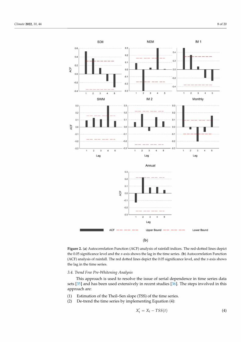
It has been mentioned that if the value of r1 is between the upper and lower bounds ofthe significance level, the time series is not serially correlated and the MK test can be applieddirectly to the time series [34]. The results obtained from the analysis of r1 displayed ahigh correlation amongst the different rainfall indices’ datasets, e.g., PRCPTOT, R20mm,and IM 1 (Figure 2a,b). Therefore, the trend-free-pre-whitening (TFPW) approach was usedto obtain the serially independent time series.

Climate 2022, 10, 44 7 of 20

Figure 2. Cont.

Climate 2022, 10, 44 8 of 20

Figure 2. (a) Autocorrelation Function (ACF) analysis of rainfall indices. The red-dotted lines depictthe 0.05 significance level and the x-axis shows the lag in the time series. (b) Autocorrelation Function(ACF) analysis of rainfall. The red dotted lines depict the 0.05 significance level, and the x-axis showsthe lag in the time series.

3.4. Trend Free Pre-Whitening Analysis

This approach is used to resolve the issue of serial dependence in time series datasets [35] and has been used extensively in recent studies [36]. The steps involved in thisapproach are:

(1) Estimation of the Theil–Sen slope (TSS) of the time series.(2) De-trend the time series by implementing Equation (4):

X′t = Xt − TSS(t) (4)

Climate 2022, 10, 44 9 of 20

Where X′t shows the de-trended series, Xt is the values of the time series at time t,and TSS(t) is the Theil–Sen slope.

(3) Test the r1 again for the detrended time series; if the value of the r1 does not reflecta serial correlation, then the MK test can be applied to the original time series dataset. Contrary to this, if the r1 shows the correlation, pre-whiten the de-trended seriesusing Equation (5):

Y′t = X′t − (r1 Xt−1) (5)

where Y′t shows the pre-whitened time series.(4) The monotonic trend is then added back to the pre-whitened time series as mentioned

in Equation (6):Y′′t = Y′t + TSS(t) (6)

where Y′′t represents the trend free pre-whitened time series.

3.5. Trend Analysis

The Mann–Kendall (MK) test has been utilized in many hydrological trend analysisstudies, for instance, the analysis of rainfall, water quality, and streamflow data [21,22].The MK test develops two hypotheses while testing the data; null (Ho) and alternativehypotheses (H1). Ho describes the no trend in time series, whereas the H1 depicts themonotonic trend in the data. The test statistics S of MK can be calculated as described byEquation 7 [37,38]:

S =n−1

∑k=1

n

∑j=k+1

sgn(xj − xk

)(7)

where n is the length of the data, xj and xk are the consecutive data values, and sgn(θ) is thesign function which can be calculated as:

Sgn (x) =

1 i f x > 00 i f x = 0−1 i f x < 0

(8)

If the variables are randomly distributed along with the independent hypotheses,the statistics S illustrates the normal distribution. In that case, the Var(S) can be calculatedusing Equation (9).

Var (S) =n(n− 1)(2n + 5)−∑n

t t(t− 1)(2t + 5)18

(9)

where n is the sample size, t is the extent of any ties, and sigma t is the sum of all tiedgroups. A tied group represents the number of sample points having the same values.The standardized test statistics Z can be determined by Equation (10):

Z =

S−1√Var (S)

f or S > 0,

0 f or S = 0,S+1√Var (s)

f or S < 0(10)

The value of Z defines the presence of trends. If the values are positive, it describesthe positive trends, whereas the negative values depict the negative trends.

3.6. Abrupt Change Analysis

The application of the MK test provides the overall positive (negative) trends; however,in order to identify the abrupt changes in rainfall indices, the sequential Mann–Kendall(SMK) test was applied.

Climate 2022, 10, 44 10 of 20

The first step in the SMK test is to calculate the sequence statistic Sk for a time series xiwhere (1 ≤ i ≤ n), using Equation (11):

Sk =k

∑i−1

ri(k = 2, 3, . . . , n) (11)

ri ={+1 i f xi > xj, 0 i f xi ≤ xj

}(j = 1, 2, . . . , i) (12)

where Sk represents the rank series; xi, xj are the data values at the time i and j, respectively;ri, on the other hand, is the rank statistics for data pairs (xi, xj) and n shows the length ofthe data series.

Like the MK test, the SMK test also draws two hypotheses, so under the null hypothe-sis, the statistics Sk is distributed as a normal distribution. Therefore, the expected value ofrank statistics and variance can be calculated as:

E(Sk) =n(n + 1)

4(13)

VAR(Sk) =n(n− 1)(2n + 5)

72(14)

In light of the assumption made above, the statistics index can be calculated as:

UFk =[Sk − E(Sk)]√

VAR(Sk)(k = 1, 2, 3, . . . , n) (15)

where UFk represents a progressive or standardized variable that has zero mean value withunit standard deviation. Therefore, its value varies around zero and the values above zeroindicate positive trends in the dataset and vice versa.

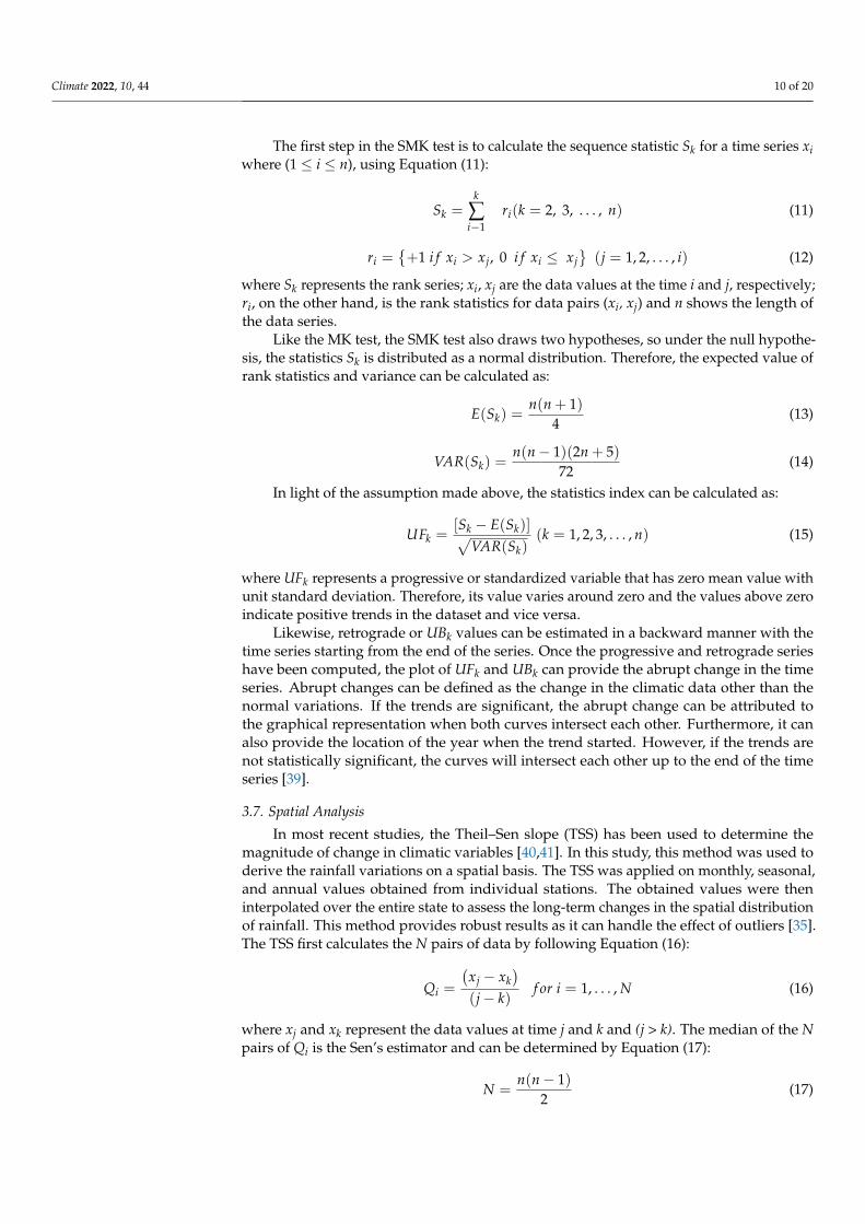
Likewise, retrograde or UBk values can be estimated in a backward manner with thetime series starting from the end of the series. Once the progressive and retrograde serieshave been computed, the plot of UFk and UBk can provide the abrupt change in the timeseries. Abrupt changes can be defined as the change in the climatic data other than thenormal variations. If the trends are significant, the abrupt change can be attributed tothe graphical representation when both curves intersect each other. Furthermore, it canalso provide the location of the year when the trend started. However, if the trends arenot statistically significant, the curves will intersect each other up to the end of the timeseries [39].

3.7. Spatial Analysis

In most recent studies, the Theil–Sen slope (TSS) has been used to determine themagnitude of change in climatic variables [40,41]. In this study, this method was used toderive the rainfall variations on a spatial basis. The TSS was applied on monthly, seasonal,and annual values obtained from individual stations. The obtained values were theninterpolated over the entire state to assess the long-term changes in the spatial distributionof rainfall. This method provides robust results as it can handle the effect of outliers [35].The TSS first calculates the N pairs of data by following Equation (16):

Qi =

(xj − xk

)(j− k)

f or i = 1, . . . , N (16)

where xj and xk represent the data values at time j and k and (j > k). The median of the Npairs of Qi is the Sen’s estimator and can be determined by Equation (17):

N =n(n− 1)

2(17)

Climate 2022, 10, 44 11 of 20

4. Results4.1. Temporal Trends in Rainfall Series

Results of MK and TSS tests are shown in Table 5, at a 5% level of significance. Positivevalues of Z suggest an increasing trend, whereas negative values indicate a decreasingtrend. From Table 5, it can be seen that most rainfall indices show weak and insignificantdownward trends. Even though during testing under the MK test, RX1Day, RX5Day, R95p,R99p, and PRCPTOT displayed insignificant trends, the rate of change was quite high whiletesting under the TSS. R95p recorded a negative growth rate of −2.30 mm/year, followedby PRCPTOT with a decline of−1.99 mm/year and R99p with a decline of−0.69 mm/year.In Perak, Malaysia, the decrease of wet spells was reflected in the negative value of Zfor the CWD. The positive MK test values for CDD, i.e., Z = 1.28 and Sen’s Slope value0.1 mm/year, indicated a rise in the number of dry spells.

Table 5. Results of MK test on rainfall indices and time series.

Indices Z p-Value Sen’s Slope (mm)

RX1Day −1.80 0.0713 −0.3067RX5Day 0.00 0.9773 0.0172

R95p −0.70 0.4955 −2.3000R99p −0.60 0.5403 −0.6947

PRCPTOT −0.40 0.6701 −1.9933R10mm 0.10 0.8982 0.0312R20mm −0.20 0.8754 0.0000

CDD 1.80 0.0759 0.1000CWD −0.60 0.5218 −0.0909SDII −0.40 0.6902 −0.0071NEM 1.10 0.2695 0.2038IM 1 0.10 0.9515 0.0246SWM −2.20 0.0299 −0.2942IM 2 −0.80 0.4410 −0.3196

Monthly −0.70 0.4661 −0.0235Annual −0.40 0.6701 −1.8293

Bold values show significance.

The bottom half of Table 5 shows the results of the MK test on the seasonal, monthly,and annual rainfall. The obtained results revealed the significant decreasing trends in theSWM at 0.05 significant level (Table 5; p = 0.0299). However, the NEM and IM 1 depictedinsignificant increasing trends. Overall, the results of annual rainfall depicted weak butdecreasing trends with the annual decrease of 1.8 mm in rainfall over Perak, Malaysia.These outcomes are contrary to that of [42], who found that there were no significant trendsin rainfall indices over Peninsular Malaysia. Further, in our case, the study was extendedto the seasonal evaluation as well, which depicted the decreasing trends in rainfall duringthe SWM season.

4.2. Sudden Changes in Rainfall Series

Figure 3a provides the results obtained from the SMK analysis of rainfall indices witha significance level of 5% (i.e., α = 0.05). The progressive or UFk curve of the RX1Dayindicated a relatively constant trend from 1980 to 1999 when it crossed the retrogradedor UBk curve indicating the trend. While a steadily decreasing trend was observed after1999 up to 2007 when it crossed the critical limit indicating the significant decreasing trend.The UFk curve of RX5Day initially portrayed the increasing trend while intersecting the UBkcurve in 1984, representing the start of a trend with some fluctuations up to 2001. It thenstarted to decrease from 2001 and crossed the critical line, which confirmed the decreasingtrends in the RX5Day index after 2006. For R95p, the UFk showed the increasing trend from1985 to 1990 but started to decrease gradually after 1990. It intersected the critical value in1995 the decreasing trends were more obvious in the year of 2008. The extreme indices of

Climate 2022, 10, 44 12 of 20

R99p and PRCPTOT illustrated somewhat the same trend during the period of 35 yearswith decreasing trend at the start of the 21st century and became significant in 2007.

Figure 3. Cont.

Climate 2022, 10, 44 13 of 20

Figure 3. (a) Results of sequential Mann–Kendall test on rainfall indices. (b) Results of sequentialMann–Kendall test on rainfall indices.

The UFk curves showed the increasing trends for the late 80′s but then started to de-crease after 1994–2014. The R10mm did not portray any significant trend as the progressiveand retrograded curves cross each other inside the upper and lower limit. It has beenmentioned by [43] that if both curves cross each other inside the critical limit, then thereis no significant change in the time series. The R20mm also depicted the same trends asR99p, i.e., increasing in the late 1980s and then decreasing trend up to 2014. The results ofSMK for CDD, as shown in Figure 3a, indicate the increasing trends of dry spells during

Climate 2022, 10, 44 14 of 20

the study period with a start from 1989, and the change was significant in 2006. In contrast,the analysis of wet spells has shown declining trends over the state.

Figure 3b presents the results of the SMK test on the seasonal, monthly, and annualrainfall. The analysis of SDII has shown decreasing trends in the precipitation intensityduring the entire study period. For NEM, the rainfall trends were increasing in the 80′s;however, they decreased slightly in 1994 and then followed a fairly constant pattern.The same phenomena were observed for IM 1, IM2. However, the UFk curve of SWMshowed the increasing trends from 1980 to 1989, but then it started to decline. The curvecrossed the critical value in 2006 and then decreased significantly. For monthly timeseries, it is evident that a significant increasing trend occurred during the 80s; however,at the end of the twentieth century, the trends started to decrease since 2005. The samephenomenon was observed for annual rainfall as well, which showed the increasing trendin 1986 and then followed the constant pattern. Later, it depicted the decreasing trend in2007–2008. As for the analysis of all these indices, the abrupt change point was detectedat the intersection of UFk and UBk curves. It can be observed that almost all the changepoints have a similar starting time. The change was started in the late 90s over the Perak,and then it started to decrease. With the start of the twenty-first century, the decrease wasmore obvious in all rainfall indices.

4.3. Variations in the Concentration of Annual Rainfall

Figure 4 compares the results obtained from the PCI analysis of annual rainfall on adecadal basis. The values of PCI vary from 7 to 20 in different regions of Perak over differenttime spans. As mentioned by the Oliver (1980), the PCI values less than 10 correspond tolow rainfall concentration, while the values ranging from 11–15 represent moderate rain-fall concentration, and the values from 16–20 indicate the irregular rainfall concentration.Conversely, the values of PCI greater than 20 exhibits a high irregularity in rainfall concen-tration. As for the explanation, the low concentration of rainfall depicts the uniformity inthe rainfall distribution, where the moderate and irregular rainfall concentration representsthe seasonality in the rainfall.

As can be seen from Figure 4, the values of PCI from 1980–1989 fluctuated from10.5–13.1. The lower values were observed over the southeastern regions (i.e., 10.6), whilehigher values were observed over the northwestern regions, i.e., 13.1 (Figure 4). The sametrends were observed for the years 1990–1999. The high concentration values were observedin the western regions, and the lower values were recorded in the southeastern regions.However, the lower values of rainfall concentration were observed over the western regionsof Perak for the years 2000–2009. Furthermore, the high irregularity over the northernareas was observed as the recorded value of PCI was 24 (Figure 4). For the last period,PCI values were detected for the half-decade (i.e., 2010–2014) due to the limitation of data.The values of annual PCI stretched from 10 to 11.5 over the western to eastern regions.It can be observed from the figure that the rainfall concentration has gradually shifted fromthe southeastern regions towards the western regions. The areas of the northeast showedmoderate irregularity in rainfall during the entire study period.

Climate 2022, 10, 44 15 of 20

Figure 4. Annual rainfall concentration index on Perak, Malaysia.

4.4. Spatial Distribution of Annual Rainfall

Figure 5 presents the results of the spatial distribution of long-term monthly, seasonal,and annual rainfall over the state from 1980 to 2014. In the case of NEM, the westernareas have observed the declination in rainfall with the rate of 0.19 mm/year, while thesoutheastern areas have experienced an increase in monsoonal rainfall at the rate of 0.56 mm(Figure 5a). The same phenomenon was noted for the IM 1 with the increase in rainfall1.03 mm (Figure 5b). However, in the case of SWM and IM 2, a decreased rainfall trend wasdiscovered over the entire state. The rate of decrease was higher for the western regions (i.e.,0.45 mm) as compared to the southern regions (i.e., 0.12 mm) for SWM (Figure 5c). Whereas,for IM 2, the rate of decrease was more (i.e., 2.12 mm) from the western regions (Figure 5d).The spatial variability of monthly rainfall has also portrayed the decreased rainfall for thewestern regions and increased for the southeastern regions (Figure 5e). On an annual basis,again, the trends were similar, and the rate of decrease in annual rainfall was 19 mm for the

Climate 2022, 10, 44 16 of 20

western regions. On the other hand, the southern regions that are happened to be situatedon flat grounds have experienced an increase in rainfall at the rate of 10 mm (Figure 5f).

Figure 5. Spatial distribution of long-term (1980–2014) seasonal, monthly, and annual rainfall ratesover Perak, Malaysia. The sub-figures (a–d) represents the NEM, IM 1, SWM, and IM2 respectively.The rate of change in seasonal rainfalls are as per the definition given in Table 3, while the sub-figures(e,f) have the units in mm/month and mm/year, respectively.

Climate 2022, 10, 44 17 of 20

5. Discussion

Rainfall provides the necessary understanding to quantify the intensity and severity ofdifferent hydrological phenomena, such as floods, droughts, river discharge, etc. Estimationof the seasonal and spatial trends of rainfall can offer valuable information not only to theclimatic scientists but also to the weather forecasters, hydrologists, and decision-makers.Therefore, the objective of this research was to assess the spatiotemporal trends of rainfall toanalyze the problem of recurrent flooding in Perak, Malaysia. The specific objectives were(i) to examine the temporal variability and unexpected trend changes in rainfall indices;and (ii) to ascertain the spatial fluctuations and periodicity in the seasonal and annualrainfall trends.

The purpose of the study was to examine the long-term trends of rainfall on a spa-tiotemporal scale, but some conclusions can be drawn based on previous research aboutseasonal and temporal variations in rainfall. Variations in rainfall trends can be related toambient air temperatures due to the fact that the warmer air holds more moisture thancooler air. Studies have shown a linear relationship between surface air temperature andrainfall. A study found that an increase in surface air temperature due to an increase inthe emission of greenhouse gasses (GHGs), ultimately intensified the rainfall pattern overthe northern hemisphere during the period from 1950 to 1999 [44]. In this context, anotherstudy stated that a change in atmospheric temperature by 7% can significantly increaseglobal rainfall [45]. Despite the fact that these studies were conducted at a global level,some of their effects can be found at the regional level, as observed by other researchers [46].

An increase in dry spells can be explained by the urban heat island (UHI) effect causedby intensive land cover changes. In a previous study, the UHI effect has been shown tocause an increase in atmospheric temperature, particularly in highly populated areas [47].A recent study analyzing the rate of land-use changes in Perak has mentioned that dur-ing the last decade, the land cover has been altered extensively in Perak, Malaysia [27].The fluctuations in local atmospheric temperatures because of the UHI effect can alter therainfall over that particular area. This can also be explained by a study done to examine theinterannual variation in temperature over entire Malaysia. Their results found that increasein temperature over entire Malaysia is constant because of the El Niño-Southern Oscillation(ENSO) cycle [47]. The ENSO cycle defines the temperature variations of the atmosphereand ocean across the East-central Equatorial Pacific. The variation ultimately directly influ-ences the world’s weather. Another recent study has also indicated that the frequency ofwet spells has been decreased significantly from 1971–2010 over entire Peninsular Malaysiabecause of El Niño events of 1982–1983 and 1997–1998 [48].

Furthermore, a gradually increasing trend in the daily minimum temperature has alsobeen observed by the Malaysian Meteorological department over the entire of Malaysia.A study has directly coincided with the increased trends in temperature with the El Niñoevents, which occurred in 1972, 1982 and 1997 [49]. On the spatial basis, the variationscan be observed over the western regions where rainfall showed decreasing trends andincreasing trends over the southeastern regions of the state on a seasonal and annual basis.Recent research has suggested that El Niño and La Niña events affect the rainfall patternson spatial as well as temporal patterns [50]. The same phenomenon was observed in theanalysis of the precipitation concentration index that revealed the convergence of rainfalltowards the southeastern regions of Perak from the western regions.

Other studies, such as Manton et al. (2001) and a study by Asian Development Bankhave also stated the increase in the sea–level from 1–3 mm/year and a decrease in rainfallsince 1960–2000 because of climate change [42]. Even though the results of these studiesindicated the decrease in rainfall, their results revealed the increase in hydrological hazards,for instance, floods, droughts, etc., over the Southeast Asian countries. Apart from climatechanges, the basic physical properties altered by human activities are also influential inincreasing the runoff generation within a watershed. Studies have indicated that factorssuch as anthropogenic changes also play an important role in flood intensification [51].Anthropogenic changes can be attributed to deforestation, expansion of croplands, industri-

Climate 2022, 10, 44 18 of 20

alization, and urbanization that consequently disrupts the river hydrology by reducing theinfiltration and water holding capacity of the river plain. World Meteorological Organiza-tion has also stated that human activities, for instance, deforestation and urbanization havestrongly influenced the biotic diversity of the globe. These changes in the ecosystem wouldsubsequently lead to increased precipitation, which will result in more severe flooding [52].The results obtained from the analysis of rainfall indices over Perak have revealed that therecent flooding was not solely due to climatic changes. Therefore, for sustainable spatialfuture planning, consideration of other factors such as deforestation, dam breakage, etc.,will also help to identify the root causes of flood intensification.

6. Conclusions

This study aimed to evaluate the spatiotemporal trends of rainfall over the state ofPerak Malaysia during the last 35 years. Trends in extreme rainfall indices along with theseasonal and annual rainfall were examined. The most obvious finding to emerge from thestudy was significant decreasing trends in the Southwest Monsoon (SWM) rainfall duringthe study period of 1980–2014. The study has also shown that most of the rainfall indicesare following insignificant decreasing trends. From the results, it was evident that thedecreasing point extreme indices were observed starting from 2005. On the spatial level,the rainfall depicted the convergence from the western regions towards the north-easternregions that are highly populated areas. The analysis of threshold rainfall indices (R99pand R95p) for flooding intensification did not portray any significant increasing trends,which imply the possibility of other factors in flood intensification. In general, it canbe concluded that rainfall over Perak, Malaysia, is following a slightly decreasing trend.The results of this study can be extended to understand the regional flooding over thePerak. A further study with more rainfall datasets focusing on the impact assessment ofEl Niño, global warming, and land-use changes on regional climate and the hydrologicalcycle is therefore suggested.

Author Contributions: M.F.H., M.R.U.M. and A.M.H. contributed to the formal analysis, methodol-ogy, investigations, and validation. M.F.H. and M.U.L. contributed to the data handling in software,examining the results, and writing—original draft preparation. M.R.U.M., A.M.H., M.U.L. and K.W.Y.contributed to the visualization, verify results, and writing and editing. All authors have read andagreed to the published version of the manuscript.

Funding: This research received no external funding for this research.

Data Availability Statement: The datasets generated or analyzed during the study are available withthe corresponding author on reasonable request.

Acknowledgments: The authors are thankful to the Department of Irrigation and Drainage (DID)Malaysia for providing the rainfall data for Perak, Malaysia. The first author is also thankful toUniversiti Teknologi PETRONAS, Malaysia, for providing financial support from the GraduateAssistantship (GA) scheme.

Conflicts of Interest: The authors declare no conflict of interest.

References1. Treloar, N.C. Deconstructing Global Temperature Anomalies: An Hypothesis. Climate 2017, 5, 83. [CrossRef]2. Mahmood, R.; Babel, M.S. Evaluation of SDSM developed by annual and monthly sub-models for downscaling temperature and

precipitation in the Jhelum basin, Pakistan and India. Theor. Appl. Climatol. 2013, 113, 27–44. [CrossRef]3. Masson-Delmotte, V.P.; Zhai, A.; Pirani, S.L.; Connors, C.; Péan, S.; Berger, N.; Caud, Y.; Chen, L.; Goldfarb, M.I.;

Gomis, M.; et al. (Eds.) IPCC, 2021: Climate Change 2021: The Physical Science Basis. Contribution of Working Group I to theSixth Assessment Report of the Intergovernmental Panel on Climate Change; Cambridge University Press: Cambridge, UK, 2021.

4. Yang, S.; Kang, T.; Bu, J.; Chen, J.; Gao, Y. Evaluating the Impacts of Climate Change and Vegetation Restoration on theHydrological Cycle over the Loess Plateau, China. Water 2019, 11, 2241. [CrossRef]

5. Tanteliniaina, M.F.R.; Chen, J.; Adyel, T.M.; Zhai, J. Elevation Dependence of the Impact of Global Warming on Rainfall Variationsin a Tropical Island. Water 2020, 12, 3582. [CrossRef]

Climate 2022, 10, 44 19 of 20

6. Huang, P.; Xie, S.-P.; Hu, K.; Huang, G.; Huang, R. Patterns of the seasonal response of tropical rainfall to global warming.Nat. Geosci. 2013, 6, 357–361. [CrossRef]

7. Liaqat, M.U.; Grossi, G.; Hasson, S.u.; Ranzi, R. Characterization of interannual and seasonal variability of hydro-climatic trendsin the Upper Indus Basin. Theor. Appl. Climatol. 2022, 147, 1163–1184. [CrossRef]

8. Nalley, D.; Adamowski, J.; Khalil, B. Using discrete wavelet transforms to analyze trends in streamflow and precipitation inQuebec and Ontario (1954–2008). J. Hydrol. 2012, 475, 204–228. [CrossRef]

9. Stocker, T. Climate Change 2013: The Physical Science Basis: Working Group I Contribution to the Fifth Assessment Report of theIntergovernmental Panel on Climate Change; Cambridge University Press: Cambridge, UK, 2014.

10. Solomon, S.; Manning, M.; Marquis, M.; Qin, D. Climate Change 2007—The Physical Science Basis: Working Group I Contribution tothe Fourth Assessment Report of the IPCC; Cambridge University Press: Cambridge, UK, 2007; Volume 4.

11. Lau, C.L.; Smythe, L.D.; Craig, S.B.; Weinstein, P. Climate change, flooding, urbanisation and leptospirosis: Fuelling the fire?Trans. R. Soc. Trop. Med. Hyg. 2010, 104, 631–638. [CrossRef]

12. Hirabayashi, Y.; Mahendran, R.; Koirala, S.; Konoshima, L.; Yamazaki, D.; Watanabe, S.; Kim, H.; Kanae, S. Global flood riskunder climate change. Nat. Clim. Chang. 2013, 3, 816–821. [CrossRef]

13. Kia, M.B.; Pirasteh, S.; Pradhan, B.; Mahmud, A.R.; Sulaiman, W.N.A.; Moradi, A. An artificial neural network model for floodsimulation using GIS: Johor River Basin, Malaysia. Environ. Earth Sci. 2012, 67, 251–264. [CrossRef]

14. Pradhan, B. Flood susceptible mapping and risk area delineation using logistic regression, GIS and remote sensing. J. Spat. Hydrol.2010, 9, 1–18.

15. Chan, N.W. Impacts of disasters and disaster risk management in Malaysia: The case of floods. In Resilience and Recovery in AsianDisasters; Springer: Berlin/Heidelberg, Germany, 2015; pp. 239–265.

16. Brakenridge, G.; Anderson, E. Satellite-Based Inundation Vectors; Dartmouth Flood Observatory, Dartmouth College: Hanover, LS,USA, 2004.

17. Pathak, P.; Kalra, A.; Ahmad, S. Temperature and precipitation changes in the Midwestern United States: Implications for watermanagement. Int. J. Water Resour. Dev. 2017, 33, 1003–1019. [CrossRef]

18. Pérez-Zanón, N.; Casas-Castillo, M.C.; Rodríguez-Solà, R.; Peña, J.C.; Rius, A.; Solé, J.G.; Redaño, Á. Analysis of extreme rainfallin the Ebre Observatory (Spain). Theor. Appl. Climatol. 2016, 124, 935–944. [CrossRef]

19. Liu, Z. Evaluation of precipitation climatology derived from TRMM Multi-Satellite Precipitation Analysis (TMPA) monthlyproduct over land with two gauge-based products. Climate 2015, 3, 964–982. [CrossRef]

20. Ahmad, I.; Zhang, F.; Tayyab, M.; Anjum, M.N.; Zaman, M.; Liu, J.; Farid, H.U.; Saddique, Q. Spatiotemporal analysis ofprecipitation variability in annual, seasonal and extreme values over upper Indus River basin. Atmos. Res. 2018, 213, 346–360.[CrossRef]

21. Krebs, G.; Camhy, D.; Muschalla, D. Hydro-Meteorological Trends in an Austrian Low-Mountain Catchment. Climate 2021, 9, 122.[CrossRef]

22. Obubu, J.P.; Mengistou, S.; Fetahi, T.; Alamirew, T.; Odong, R.; Ekwacu, S. Recent Climate Change in the Lake Kyoga Basin,Uganda: An Analysis Using Short-Term and Long-Term Data with Standardized Precipitation and Anomaly Indexes. Climate2021, 9, 179. [CrossRef]

23. Wong, C.; Venneker, R.; Uhlenbrook, S.; Jamil, A.; Zhou, Y. Variability of rainfall in Peninsular Malaysia. Hydrol. Earth Syst. Sci.Discuss. 2009, 6, 5471–5503.

24. Suhaila, J.; Jemain, A.A. Spatial analysis of daily rainfall intensity and concentration index in Peninsular Malaysia. Theor. Appl.Climatol. 2012, 108, 235–245. [CrossRef]

25. Amirabadizadeh, M.; Huang, Y.F.; Lee, T.S. Recent trends in temperature and precipitation in the Langat River Basin, Malaysia.Adv. Meteorol. 2015, 2015, 579437. [CrossRef]

26. Chabala, L.M.; Kuntashula, E.; Kaluba, P. Characterization of temporal changes in rainfall, temperature, flooding hazard and dryspells over Zambia. Univers. J. Agric. Res. 2013, 1, 134–144. [CrossRef]

27. Hanif, M.F.; ul Mustafa, M.R.; Hashim, A.M.; Yusof, K.W. Spatio-temporal change analysis of Perak river basin using remotesensing and GIS. In Proceedings of the 2015 International Conference on Space Science and Communication (IconSpace),Langkawi, Malaysia, 10–12 August 2015; pp. 225–230.

28. Bargaoui, Z.K.; Chebbi, A. Comparison of two kriging interpolation methods applied to spatiotemporal rainfall. J. Hydrol. 2009,365, 56–73. [CrossRef]

29. Verdin, A.; Funk, C.; Rajagopalan, B.; Kleiber, W. Kriging and local polynomial methods for blending satellite-derived andgauge precipitation estimates to support hydrologic early warning systems. IEEE Trans. Geosci. Remote Sens. 2016, 54, 2552–2562.[CrossRef]

30. Stefanidis, S.; Stathis, D. Spatial and temporal rainfall variability over the Mountainous Central Pindus (Greece). Climate 2018,6, 75. [CrossRef]

31. Oliver, J.E. Monthly precipitation distribution: A comparative index. Prof. Geogr. 1980, 32, 300–309. [CrossRef]32. de Luis, M.; Gonzalez-Hidalgo, J.; Brunetti, M.; Longares, L. Precipitation concentration changes in Spain 1946–2005. Nat. Hazards

Earth Syst. Sci. 2011, 11, 1259–1265. [CrossRef]33. Thomas, J.; Prasannakumar, V. Temporal analysis of rainfall (1871–2012) and drought characteristics over a tropical monsoon-

dominated State (Kerala) of India. J. Hydrol. 2016, 534, 266–280. [CrossRef]

Climate 2022, 10, 44 20 of 20

34. Sayemuzzaman, M.; Jha, M.K. Seasonal and annual precipitation time series trend analysis in North Carolina, United States.Atmos. Res. 2014, 137, 183–194. [CrossRef]

35. Yue, S.; Pilon, P.; Cavadias, G. Power of the Mann–Kendall and Spearman’s rho tests for detecting monotonic trends in hydrologicalseries. J. Hydrol. 2002, 259, 254–271. [CrossRef]

36. Önöz, B.; Bayazit, M. Block bootstrap for Mann–Kendall trend test of serially dependent data. Hydrol. Processes 2012, 26, 3552–3560.[CrossRef]

37. Kendall, M.G. Rank Correlation Methods; University of Michigan: Ann Arbor, MI, USA, 1948.38. Mann, H.B. Nonparametric tests against trend. Econom. J. Econom. Soc. 1945, 13, 245–259. [CrossRef]39. Mohsin, T.; Gough, W.A. Trend analysis of long-term temperature time series in the Greater Toronto Area (GTA). Theor. Appl.

Climatol. 2010, 101, 311–327. [CrossRef]40. Quansah, J.E.; Naliaka, A.B.; Fall, S.; Ankumah, R.; Afandi, G.E. Assessing Future Impacts of Climate Change on Streamflow

within the Alabama River Basin. Climate 2021, 9, 55. [CrossRef]41. Amarouche, K.; Akpınar, A. Increasing Trend on Storm Wave Intensity in the Western Mediterranean. Climate 2021, 9, 11.

[CrossRef]42. Manton, M.J.; Della-Marta, P.M.; Haylock, M.R.; Hennessy, K.; Nicholls, N.; Chambers, L.; Collins, D.; Daw, G.; Finet, A.;

Gunawan, D. Trends in extreme daily rainfall and temperature in Southeast Asia and the South Pacific: 1961–1998. Int. J. Climatol.2001, 21, 269–284. [CrossRef]

43. Guo, L.; Xia, Z. Temperature and precipitation long-term trends and variations in the Ili-Balkhash Basin. Theor. Appl. Climatol.2014, 115, 219–229. [CrossRef]

44. Min, S.-K.; Zhang, X.; Zwiers, F.W.; Hegerl, G.C. Human contribution to more-intense precipitation extremes. Nature 2011, 470,378–381. [CrossRef]

45. Westra, S.; Alexander, L.V.; Zwiers, F.W. Global increasing trends in annual maximum daily precipitation. J. Clim. 2013, 26,3904–3918. [CrossRef]

46. Sato, T.; Kimura, F.; Kitoh, A. Projection of global warming onto regional precipitation over Mongolia using a regional climatemodel. J. Hydrol. 2007, 333, 144–154. [CrossRef]

47. Tangang, F.; Juneng, L.; Ahmad, S. Trend and interannual variability of temperature in Malaysia: 1961–2002. Theor. Appl. Climatol.2007, 89, 127–141. [CrossRef]

48. Zin, W.Z.W.; Jamaludin, S.; Deni, S.M.; Jemain, A.A. Recent changes in extreme rainfall events in Peninsular Malaysia: 1971–2005.Theor. Appl. Climatol. 2010, 99, 303–314. [CrossRef]

49. Sammathuria, M.; Ling, L. Regional climate observation and simulation of extreme temperature and precipitation trends.In Proceedings of the 14th International Rainwater Catchment Systems Conference, Kuala Lumpur, Malaysia, 3–6 August 2009;pp. 3–6.

50. Portmann, R.W.; Solomon, S.; Hegerl, G.C. Spatial and seasonal patterns in climate change, temperatures, and precipitation acrossthe United States. Proc. Natl. Acad. Sci. USA 2009, 106, 7324–7329. [CrossRef] [PubMed]

51. Kundzewicz, Z.; Schellnhuber, H.-J. Floods in the IPCC TAR perspective. Nat. Hazards 2004, 31, 111–128. [CrossRef]52. Ramesh, A. Response of Flood Events to Land Use and Climate Change: Analyzed by Hydrological and Statistical Modeling in Barcelonnette,

France; Springer Science & Business Media: Berlin/Heidelberg, Germany, 2012.