Lithos 120 (2010) 14–29

Contents lists available at ScienceDirect

Lithos

j ourna l homepage: www.e lsev ie r.com/ locate / l i thos

Europe from the bottom up: A statistical examination of the central and northernEuropean lithosphere–asthenosphere boundary from comparing seismologicaland electromagnetic observations

Alan G. Jones a,⁎, Jaroslava Plomerova b, Toivo Korja c, Forough Sodoudi d, Wim Spakman e

a Dublin Institute for Advanced Studies, 5 Merrion Square, Dublin 2, Irelandb Geophysical Institute, Czech Academy of Sciences, 141 31 Prague 4, Czech Republicc Geophysics Group, Department of Physical Sciences, University of Oulu, P.O.B. 3000, FI-90014, Oulu, Finlandd Helmholtz Centre Potsdam, GFZ German Research Centre for Geosciences, Telegrafenberg, 14473 Potsdam, Germanye Department of Earth Sciences, Faculty of Geosciences, Utrecht University, P.O. box 80021, 3508 TA Utrecht, The Netherlands

⁎ Corresponding author.E-mail addresses: alan@cp.dias.ie (A.G. Jones), jpl@ig

toivo.korja@oulu.fi (T. Korja), foroug@gfz-potsdam.de ((W. Spakman).

0024-4937/$ – see front matter © 2010 Elsevier B.V. Adoi:10.1016/j.lithos.2010.07.013

a b s t r a c t

a r t i c l e i n f o

Article history:Received 12 October 2009Accepted 19 July 2010Available online 24 July 2010

Keywords:Lithosphere–asthenosphere boundary (LAB)EuropeSeismologyMagnetotellurics

The Lithosphere–Asthenosphere Boundary (LAB) is a fundamental boundary in the plate tectonic paradigm—

it is the most pervasive on the planet, yet comparatively it is one we know little about. Defined initiallyon the basis of the mechanical response of the Earth to loading, its usage has become ubiquitous acrossthe geosciences but the natural differences in its definition, due to differences in thermal, physical andchemical parameters, cause confusion. To advance this debate, comparisons are made both qualitatively andquantitatively, between the delineation of the LAB for Europe based on seismological and electromagneticobservations.We examine statistically, using robustmethods, the LABs derived from independent datasets andmethods.Essentially, all definitions of the LAB, as an impedance contrast from receiver functions (sLABrf), a seismicanisotropy change (sLABa) and an increase in conductivity from magnetotellurics (eLAB), are consistentwith a deeper LAB beneath Precambrian Europe, and a shallower LAB beneath Phanerozoic Europe, withsome exceptionally deep regions in Phanerozoic Europe, such as the Alps. All three LABs increase in depthsignificantly and rapidly at a location consistent with the surface expression of the Trans-European SutureZone (TESZ) which separates Precambrian Europe to the north and east from Phanerozoic Europe in thecentre. Two of the definitions, sLABrf and eLAB, are consistent for Phanerozoic Europe with mean values of90–100 km, compared to an average sLABrf of 135 km. A different two, sLABa and sLABrf, are consistent forPrecambrian Europe with mean values of 170–180 km compared to an eLAB mean of 250 km. The deepereLAB depths for Precambrian Europe are more consistent with body wave and surface wave tomographymodels than are the sLABa and sLABrf ones, suggesting that the lower lithosphere beneath PrecambrianEurope between 170 to 250 km is responding to shearing on the base of the lithosphere from plate drivingforces.Taken together the definitions provide strong constraints on the nature of the LAB. For example, theelectrical eLAB beneath the TESZ is anomalously thick, to possibly the transition zone, whereas sLABa andsLABrf seismological definitions would place it at far shallower depths. Given the sensitivity of electricalconductivity to partial melt and water content, the thick eLAB beneath the TESZ excludes interpretation ofthe seismic LAB in that location in terms of a thermal structure that would induce partial melting or ofhydration.

.cas.cz (J. Plomerova),F. Sodoudi), wims@geo.uu.nl

ll rights reserved.

© 2010 Elsevier B.V. All rights reserved.

1. Introduction

The boundary between the Lithosphere and Asthenosphere, theLAB, is a fundamental boundary in the plate tectonic paradigm

separating the rigid material of the plates from ductile convectingmaterial below on which the plates ride. It is the most extensive onthe planet, exists beneath both oceans and continents, yet perverselyit is the boundary that comparatively we know little about (Eatonet al., 2009; Romanowicz, 2009; Fischer et al., 2010), but whendiscussed is one that is too readily assumed to be understood. Thedifficulty of its identification is compounded by the differentgeophysical and geochemical proxies used (Eaton et al., 2009), all ofwhich are sensitive to variations in different physical or chemical

15A.G. Jones et al. / Lithos 120 (2010) 14–29

properties. Certainly, the recent global compilation of the depth to theLAB based on imaging P-to-S converted phases by Rychert andShearer (2009) with an “LAB” at 95±4 km beneath Precambrianregions is seriously at odds with almost all other geophysicaldefinitions and with petrological observations, highlighting theproblem of definitive attribution of a boundary to an imagedgeophysical or geochemical interface.

Artemieva (2009) recently provided an excellent summary of thedifferent types of LAB, with three broad definitions in terms of aMechanical Boundary Layer (MBL), a Thermal Boundary Layer (TBL)and a Chemical Boundary layer (CBL, or geochemically-definedContinental Lithosphere, CL, (Anderson, 1995)). Generally, the MBLis about half the thickness of the other two (Artemieva, 2009), and onoccasion the TBL and CBL concur. However, the CBL can exhibitspatially rapid depth variations which are inherently excluded in anyTBL observations as the thermal field naturally is diffusive in natureand strong lateral thermal contrasts can only be maintained ongeologically short time-scales.

To further our understanding of the nature of the LAB and of theinter-relationships between some of the various geophysical proxies,we compare and contrast depths to the LAB derived from seismolog-ical and electromagnetic observations across Europe. This paper is notintended to be an exhaustive review of the LAB beneath Europe, butrather an objective comparison of estimates of depths to the LAB andtheir inter-relationships, using robust statistical techniques, from twoseismological methods and from magnetotellurics (MT). As such, weview our work as the first step in what must become a global effort tocompare and contrast LAB estimates from a multitude of techniques ifwe are to further our understanding of the nature of the LAB.

Begging the question of the nature of the LAB is our definitions ofthe lithosphere and asthenosphere themselves, without which wecannot define the LAB. Generally, for the purpose of our comparisonwe define the lithosphere as (cold) electrically resistive, seismically

Fig. 1. Age domain map of Europe (from

fast material with an anisotropy direction often different frompresent-day absolute plate motion (APM), whereas the astheno-sphere is (hot) electrically conductive, seismically slow material withan anisotropy direction parallel to APM (e.g., Eaton et al., 2009). Thetechniques we use to image the Earth employ seismic and electro-magnetic waves, and are thus primarily sensitive to strong temper-ature variation (e.g., Jones et al., 2009), so we are generally imagingthe depth to the TBL, rather than to the MBL or CBL.

Fig. 1 shows a generalized age domain map of Europe fromArtemieva (pers. comm.). The dominant tectonic feature of Europe,besides the topographic feature of the Alps, is the Trans-EuropeanSuture Zone (TESZ) that separates predominantly Phanerozoic Europeto the southwest from predominantly Precambrian Europe to thenortheast. The TESZ is a fundamental boundary in the LAB that showsup in all of the proxies, albeit with differing estimates of thecontrasting depths to the LAB across it, and the rapid change in thedepth to the LAB has been observed in many geophysical studies,particularly as part of focussed seismological and electromagneticexperiments of the TESZ, e.g., TOR, CEMES, POLONAISE and CELEBRA-TION (e.g., Gregersen et al., 2002; Plomerova et al., 2002a; Guterchand Grad, 2006; Pushkarev et al., 2007; Semenov et al., 2008; Smirnovand Pedersen, 2009; Wilde-Piorko et al., 2010).

Within both Phanerozoic and Precambrian Europe there aresignificant lateral variations in the depth to the LAB, particularlyassociated with Alpine subduction. In general, the variations inPrecambrian Europe are smoother, except for the western andnorthern boundaries towards the oceans and the southern boundarytowards the TESZ.

As we will show, our estimators of the depths to the LAB arenowhere all three consistent with one another — in PhanerozoicEurope two of them agree with each another, to within statisticalerror, whereas in Precambrian Europe a different two of them agree.From these similarities and differences lies information about the

I. Artemieva, 2008, pers. comm.).

16 A.G. Jones et al. / Lithos 120 (2010) 14–29

nature of the LAB, with the strong inference that it is not the same atall places.

2. Estimates of the depth to the LAB in Europe

2.1. Seismic anisotropy LAB — sLABa

Plomerova, Babuska and colleagues (Babuska and Plomerova,1992; Plomerova et al., 2002b) define the LAB as the depth at whichseismic anisotropy direction changes from a lithospheric “fossil”direction to an asthenospheric plate-flow direction parallel to APM.Herein we term these the “sLABa” estimates. Changes in orientation ofanisotropy intensify the P-velocity contrast above and below the LAB,and are reflected in radial and azimuthal anisotropy of surface waves.A full description of the analysis approach and the results obtained forEurope is given in a companion paper in this volume (Plomerova andBabuska, 2010), to which the interested reader is referred. Forcompleteness, below we give a short description of the Strengths andWeaknesses of all methods.

2.1.1. StrengthsThe strength of this single station method, based on an empirical

relation between relative P-wave travel time delays (residuals) andthe LAB depths, is in its sensitivity to lateral changes of lithosphericthickness, which is independent of region parameterization. Theaccuracy of the mean representative residuals is usually better than±0.1 s, which allows us to estimate the sLABa depth variations with anaccuracy of~±10 km. Considering steep rays used to calculate staticterms of the relative residuals, the station means represent volumeswith radii of about 25, 40 and 60 km at depths 50, 100 and 150 km,respectively. No a priori velocity–depth distribution in the uppermantle is required (Babuska and Plomerova, 1992).

Fig. 2. Estimates of the depth to the seismic anisotropically defined LAB, the sLABa, fromPlomerova et al. (2008) and Plomerova and Babuska (2010).

2.1.2. WeaknessesThe sLABa estimates require good knowledge of the structure of

the crust—P-velocity and Moho depth, and especially thickness andvelocity of a sedimentary cover if present beneath a station. Only afterapplying proper time corrections for crustal effects can the variationsof the P residuals be associated with variations of the sLABa depths. Alimitation can come from considering the “LAB depth-P-residual”relation constant at provinces of different ages with potentiallydifferent inclinations of lithospheric mantle fabrics (Babuska et al.,1998).

2.1.3. Results for EuropeThis seismic anisotropy LAB, sLABa, was mapped across Europe

using the data from a variety of seismic experiments (Plomerova et al.,2002a; Babuska and Plomerova, 2006; Plomerova et al., 2006, 2008;Plomerova and Babuska, 2010). The sLABa estimates for Europe areshown in Fig. 2, and in histogram form in Fig. 8. The minimum andmaximum values are 32 km (beneath the Danish Basin) and 250 km(northwestern Alps), with the mean of the 657 estimates being

sLABa = 137� 48km:

(Note: all statistical estimates of various subsets are shown inTable 1.)

We can obtain robust estimates of the mean and range by usingoutlier rejection. Rejecting the 10 points that lie outside the 95%confidence limits of 42–232 km yields a mean and range of

sLABa = 138� 46km:

However, a statistical test for unimodality, namely ‘diptst1’ ofHartigan (1985) based onHartigan andHartigan (1985)with F.Mechlerand Y. Lu's corrections, yields a dip statistic of 0.034, inferring that there

Plomerova et al. (2002a), Babuska and Plomerova (2006), Plomerova et al. (2006),

Table 1Statistical estimates of the depth to the lithosphere–asthenosphere boundary from thedifferent techniques and subsets.

sLABa [km] sLABrf [km] eLAB [km]

All 137±48 106±34 170±112Within 95% of mean 138±46 96±18 153±95LABsb150 km 100±27 78±28LABsN150 km 183±19 250±51Phanerozoica 118±45 96±17 98±56–Median smoothedb 133±49 89±49Precambrian 169±35 172±26 237±66–Median smoothed 182±13 253±29

a Alps excluded.b Northern Germany excluded.

17A.G. Jones et al. / Lithos 120 (2010) 14–29

is more than one peak in the depth distribution, as is visually evident inFig. 8. The sLABa estimates have two peaks, one at around 80–100 kmand the other at around 180–200 km, so themean sLABa of all values ismeaningless as it actually lies within the minimum between these twopeaks. Splitting the sLABa depth estimates into two groups, b150 kmand N150 km, the means of the two groups are

sLABab150 = 100� 27km; and sLABaN150 = 183� 19km

with the shallower depths (red circles, Fig. 10) representative ofpredominantly Phanerozoic Europe and the deeper depths (bluecircles, Fig. 10) of Precambrian Europe and the Alpine region. Notethat, as would be expected, splitting the sLABa depths into shallowand deep groups significantly reduced deviations (variance) of theaverages—from 46 km for the combined average to 27 and 19 km,respectively. For Phanerozoic Europe, excluding the Alps, and forPrecambrian Europe, the averages and ranges are

sLABaPhan = 118� 45km; and sLABaPrecam = 169� 35km:

Fig. 3.Median smoothed sLABa estimates, sLABam, of Fig. 2. Smoothing by median filtering uand a tension of 0.5.

To avoid issues related to data sampling biases, the sLABaestimates were smoothed using the Generic Mapping Tools (GMT)function blockmedian with a width of 2 degrees and a tension of 0.5.The 108 estimates are shown in Fig. 3, and in histogram form in Fig. 9.Fig. 3 more strikingly displays the shallow sLABa beneath the Danishand North German Sedimentary Basins, the shallower sLABa on theNorwegian coast, and the deep sLABa beneath the central part of theBaltic Shield in Finland. The smoothing minimizes the extent of thePannonian Basin as a result of the fact that the basin is surrounded bythe deep lithosphere beneath the Carpathians and the Eastern Alps. Ifthe shallow values for the Danish and North German SedimentaryBasins are excluded, then the averages for Phanerozoic and Precam-brian Europe become

Phanerozoic Europe

sLABam = 133 � 49km;

Precambrian Europe

sLABam = 182 � 13 km:

The TESZ is visible in both single value and smoothed sLABa depthimages (Figs. 2 and 3)with a strong change in the depth to the LAB. Thisstep-like change of ~100 km is greater than the difference between thetwo mean values between Phanerozoic and Precambrian Europe.

2.2. Seismic S-wave receiver function LAB — sLABrf

The S-to-P receiver function (SRF) technique is a relatively newtechnique that is capable of identifying especially the LAB over themore conventional P-to-S RF method (PRF) (Yuan et al., 2006). ThePRF method is not as sensitive to the LAB given the velocity inversion

sing the Generic Mapping Tools (GMT) function blockmedianwith a width of 2 degrees

18 A.G. Jones et al. / Lithos 120 (2010) 14–29

that occurs with slower velocities in the upper asthenosphere andfaster velocities in the lower lithosphere. The SRF technique has beenused in many tectonic settings (Kumar et al., 2005; Sodoudi et al.,2006a, b; Heit et al., 2007; Sodoudi et al., 2009) and results haverecently been produced for Europe (Geissler et al., 2010), to which theinterested reader should refer for more detailed description. Rychertet al. (2010) provide a recent global compilation of both PRF and SRFresults and a discussion of the strengths and weaknesses of the RFmethod. The results for Europe from Geissler et al. (2010) areanalysed here, and are termed the “sLABrf” estimates.

2.2.1. StrengthsThemost significant strength of this technique is that SRFs are very

sensitive to rapid impedance contrasts, and can therefore inferimportant information about the abruptness of the LAB. SRFmodellingshows that generally the LAB is relatively sharp with an overallsharpness of less than 20 km (Li et al., 2007; Kawakatsu et al., 2009;Rychert and Shearer, 2009). Moreover, the SRFs are not biased bycrustal multiple conversions as are P-to-S receiver functions (PRFs).The S receiver function technique is successful in observing the LABwith high resolution and density and has the potential to gain thesame significance for the lower lithosphere as steep angle seismics forthe upper lithosphere.

2.2.2. WeaknessesOne general weakness of RFs is that they require an accurate

velocity model to convert from time to depth, which is providedthrough other seismological techniques. Taking into consideration themaximum depth resolution of the SRF as well as possible bias errordue to the reference model used, an error of±10 km must beconsidered in sLABrf depth estimates.

The presence of thick sedimentary layers must be considered inestimating the LAB depth. However, regarding the error (~10 km)

Fig. 4. Estimates of the depth to the S-to-P define

introduced in the sLABrf depth estimation, and due to the lack ofreliable local velocity models, this effect has been neglected in thestudy of Geissler et al. (2010).

2.2.3. Results for EuropeThe sLABrf estimates derived by Geissler et al. (2010) at 47

locations in predominantly central Europe are shown in Fig. 4. Themean of the sLABrf estimates is

sLABrf = 106� 34km:

Rejecting the 5 points that lie outside the 95% confidence limits of37–174 km yields a mean of

sLABrf = 96� 18km:

The rejected values are those that lie to the northeast, i.e., north ofthe TESZ. Thus, this robust average sLABrf estimate is valid for centralPhanerozoic Europe.

Themedian-smoothedsLABrf estimates (sLABrfm)are shown inFig. 5,and the variation across the TESZ is clearlymarked in these estimates. Theaverages and standard deviations on either side of the TSZ are:

Phanerozoic Europe

sLABrfm = 96� 17km 26valuesð Þ;

Precambrian Europe

sLABrfm = 172� 26km 5valuesð Þ:

In terms of the nature of the LAB, Geissler et al. (2010) found asharp LAB beneath the Phanerozoic platform of Central Europe, but

d LAB, the sLABrf, from Geissler et al. (2010).

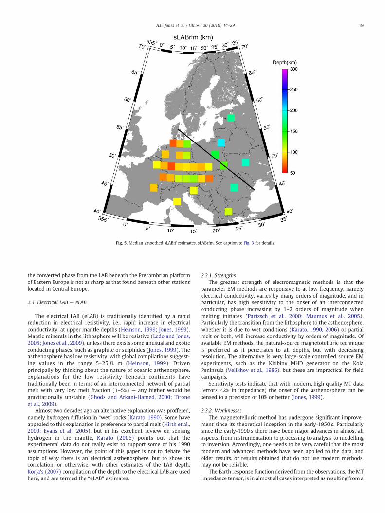
Fig. 5. Median smoothed sLABrf estimates, sLABrfm. See caption to Fig. 3 for details.

19A.G. Jones et al. / Lithos 120 (2010) 14–29

the converted phase from the LAB beneath the Precambrian platformof Eastern Europe is not as sharp as that found beneath other stationslocated in Central Europe.

2.3. Electrical LAB — eLAB

The electrical LAB (eLAB) is traditionally identified by a rapidreduction in electrical resistivity, i.e., rapid increase in electricalconductivity, at upper mantle depths (Heinson, 1999; Jones, 1999).Mantle minerals in the lithosphere will be resistive (Ledo and Jones,2005; Jones et al., 2009), unless there exists some unusual and exoticconducting phases, such as graphite or sulphides (Jones, 1999). Theasthenosphere has low resistivity, with global compilations suggest-ing values in the range 5–25 Ω m (Heinson, 1999). Drivenprincipally by thinking about the nature of oceanic asthenosphere,explanations for the low resistivity beneath continents havetraditionally been in terms of an interconnected network of partialmelt with very low melt fraction (1–5%) — any higher would begravitationally unstable (Ghods and Arkani-Hamed, 2000; Tironeet al., 2009).

Almost two decades ago an alternative explanation was proffered,namely hydrogen diffusion in “wet” rocks (Karato, 1990). Some haveappealed to this explanation in preference to partial melt (Hirth et al.,2000; Evans et al., 2005), but in his excellent review on sensinghydrogen in the mantle, Karato (2006) points out that theexperimental data do not really exist to support some of his 1990assumptions. However, the point of this paper is not to debate thetopic of why there is an electrical asthenosphere, but to show itscorrelation, or otherwise, with other estimates of the LAB depth.Korja's (2007) compilation of the depth to the electrical LAB are usedhere, and are termed the “eLAB” estimates.

2.3.1. StrengthsThe greatest strength of electromagnetic methods is that the

parameter EM methods are responsive to at low frequency, namelyelectrical conductivity, varies by many orders of magnitude, and inparticular, has high sensitivity to the onset of an interconnectedconducting phase increasing by 1–2 orders of magnitude whenmelting initiates (Partzsch et al., 2000; Maumus et al., 2005).Particularly the transition from the lithosphere to the asthenosphere,whether it is due to wet conditions (Karato, 1990, 2006) or partialmelt or both, will increase conductivity by orders of magnitude. Ofavailable EM methods, the natural-source magnetotelluric techniqueis preferred as it penetrates to all depths, but with decreasingresolution. The alternative is very large-scale controlled source EMexperiments, such as the Khibiny MHD generator on the KolaPeninsula (Velikhov et al., 1986), but these are impractical for fieldcampaigns.

Sensitivity tests indicate that with modern, high quality MT data(errors b2% in impedance) the onset of the asthenosphere can besensed to a precision of 10% or better (Jones, 1999).

2.3.2. WeaknessesThe magnetotelluric method has undergone significant improve-

ment since its theoretical inception in the early-1950 s. Particularlysince the early-1990 s there have been major advances in almost allaspects, from instrumentation to processing to analysis to modellingto inversion. Accordingly, one needs to be very careful that the mostmodern and advanced methods have been applied to the data, andolder results, or results obtained that do not use modern methods,may not be reliable.

The Earth response function derived from the observations, theMTimpedance tensor, is in almost all cases interpreted as resulting from a

20 A.G. Jones et al. / Lithos 120 (2010) 14–29

uniform source field. Major effort is expended by MT specialists whendealing with time series that may be contaminated by non-uniformsource field structure (Jones and Spratt, 2002; Varentsov et al., 2003).Generally, the effects will lead to an underestimate in the depth to theLAB (see Jones and Spratt, 2002), although that is not always the case(Jones, 1980).

In addition, some of the eLAB estimates comes from single site 1Dinversions (see Korja, 2007 for details) so may suffer from the effectsof static shifts (see, e.g., Jones, 1988). However, the compilation reliedon the results from more sophisticated 2D models where available.

2.3.3. Results for EuropeRecently, Korja (2007) assessed estimates of eLAB depths provided

by interpretations of primarily magnetotelluric data from a widerange of experiments held across Europe, and critically selected thosein which he had confidence. The 245 eLAB estimates for Europe inKorja's database are shown in Fig. 6, and block averaged in Fig. 7. Theminimum and maximum values are 20 km (Apennines) and 410 km(N of TESZ). These LAB estimates clearly have the largest range of thethree estimators, and the mean, with its significantly large standarddeviation, is

eLAB = 170� 112km:

Rejecting the 17 points that lie outside the 95% confidence limits of0–394 km, i.e., all of those with default values of 400 km or 410 km,yields a mean of

eLAB = 153� 95km:

The statistical test for unimodality yields a dip statistic of 0.041confirmingwhat is visually obvious in Figs. 6, 8 and 9 that there is morethan one peak in the eLAB depth distribution, with one strong shallow

Fig. 6. Estimates of the depth to the electrically

peak at 60–80 km and a broader deeper peak centred on 240–260 km.Thus, as with the sLABa, the mean is meaningless and lies between twopeaks in the distribution. Splitting the eLAB depth estimates into twogroups, b150 km and 150–350 km, the means of the two groups are

eLABb150 = 78� 28km; and eLAB150−350 = 250� 51km

with the shallower depths (green squares, Fig. 10) representative ofPhanerozoic Europe and the deeper depths (purple squares, Fig. 10) ofpredominantly Precambrian Europe. Splitting the database into twogroups by age of crustal rocks, as shown in Fig. 1, excluding the Alpsand the ultra-deep values north of the TESZ, yields the means andspreads for Phanerozoic and Precambrian Europe

eLABPhan = 98� 56km; and eLABPrecam = 237� 66km:

The anomalously deep values of the depth to the first mantleconductor of around 350–400 km just north of the TESZ is best seen inthe very careful work of Smirnov and Pedersen (2009), who studiedthe Sorgenfrei–Tornquist Zone branch of the TESZ in southern Swedenand Denmark. Such resistive mantle to effectively the transition zoneis very surprising, and these cannot be considered depths to the“LABs”—essentially there is no evidence of an electrical asthenospherebeneath and directly to the north of the TESZ. On their own, onemightbe tempted to discount these deep depths as due to inappropriateanalysis and modelling, and invoke effects such as source fieldcontamination, although non-uniform source fields will generally biasLAB estimates to shallower levels (e.g., Jones and Spratt, 2002).However, a recent analysis of annual means from European magneticobservatory data by Dobrica and Demetrescu (2009) for very longperiod/deeply-penetrating information showed a NW–SE strip of highresistivity/high inductance through Europe that is spatially coincidentwith the location of the TESZ. Such high resistivities imaged by

-defined LAB, the eLAB, from Korja (2007).

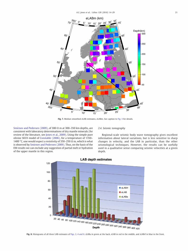
Fig. 7. Median smoothed eLAB estimates, eLABm. See caption to Fig. 3 for details.

21A.G. Jones et al. / Lithos 120 (2010) 14–29

Smirnov and Pedersen (2009), of 300 Ωm at 300–350 km depths, areconsistent with laboratory determinations of dry mantle minerals (forreview of the literature, see Jones et al., 2009). Using the simple pureolivine SEO3 model of Constable (2006), for a temperature of 1350–1400 °C, onewould expect a resistivity of 350–250 Ωm,which is whatis observed by Smirnov and Pedersen (2009). Thus, on the basis of theEM results we can exclude any suggestion of partial melt or hydrationof the upper mantle in this region.

Fig. 8. Histograms of all three LAB estimates of Figs. 2, 4 and 6. sLABa in gree

2.4. Seismic tomography

Regional-scale seismic body wave tomography gives excellentinformation about lateral variations, but is less sensitive to sharpchanges in velocity, and the LAB in particular, than the otherseismological techniques. However, the results can be usefullyused in a qualitative sense comparing seismic velocities at a givendepth.

n at the back, eLAB in red in the middle, and sLABrf in blue in the front.

Fig. 9. Histograms of all three median smoothed LAB estimates of Figs. 3, 5 and 7. sLABam in green at the back, eLABm in red in the middle, and sLABrfm in blue in the front.

22 A.G. Jones et al. / Lithos 120 (2010) 14–29

2.4.1. StrengthsThe greatest strength of body wave tomography is its ability to

sense both lateral and vertical variations in seismic velocity, albeitwith differing resolution.

2.4.2. WeaknessesOne weakness of body wave topographic methods is the

prevalence for vertical smearing of structures along arrival paths,

Fig. 10. Shallow (b150 km) and deep (N150 km) LAB estimates. Shallow sLABa estimates argreen, and deep eLAB estimates are in purple.

especially in regions of poor ray coverage. Also length-scale ofmapping of lateral variations is restricted to horizontal parameterisa-tion of the velocity model (size of blocks or node spacing).

2.4.3. Results for EuropeFig. 11 displays a slice at 260 km depth from the new body wave

tomographic model of Europe from Spakman (unpubl.) using thetravel time information for Europe of Amaru et al. (2008). The original

e dots in red, and deep sLABa estimates in blue. Shallow eLAB estimates are squares in

Fig. 11. Seismic Vp absolute velocity at 260 km depth from Spakman (unpubl.). Original velocity anomaly map in percent was converted to velocity using a value of 8.48 km/s, whichis the Vp velocity at 250 km from ak135.

Fig. 12. Cross-plot of raw sLABrf estimates against raw sLABa estimates for locationsthat are within 25 km of each other. The solid black line is the 1:1 line that the datashould scatter around if there are no bias errors. The dotted line is a linear regressionanalysis, assuming both sets of data are in error. The dashed line is a robust linearregression with outlier rejection.

23A.G. Jones et al. / Lithos 120 (2010) 14–29

model velocity data were in percentage differences from a standardmodel, namely ak135 (Kennett et al., 1995). The data have beenadjusted relative to a velocity of 8.48 km/s, the velocity at 260 km inak135, and plotted as absolute velocity in Fig. 11. This depth waschosen as to be below most estimates of the LAB. The TESZ is clearlyvisible at 260 km separating a southern region of velocity below8.5 km/s from a northern region with velocity above 8.5 km/s.

3. Quantitative statistical comparisons of LAB estimates

3.1. sLABrf cf. sLABa

Fig. 12 shows a cross-plot between 35 sLABrf and sLABa depthestimates, for observation locations that are within 25 km of eachother. If both estimators are unbiased, they would scatter around the1:1 solid black line, whereas clearly the majority of points lie abovethe 1:1 line inferring that sLABa estimates are systematically largerthan sLABrf estimates. A linear regression analysis, assuming both setsof data are in error (York, 1966; 1969; Fasano and Vio, 1988), of the 35points yields

sLABa = −84:1 �1:7ð Þ + 2:08 �0:02ð ÞTsLABrf kmð Þ;

(dotted black line) with a correlation coefficient of only 0.59. Usingrobust statistics to identify and reject outliers (Huber, 1981), the twostatistical “outlier” values at large sLABrf/sLABa are downweightedand a robust York-Fasano linear regression gives

sLABa = −108:5 �2:3ð Þ + 2:38 �0:02ð ÞTsLABrf kmð Þ;

(dashed black line) with a correlation coefficient of 0.86.

A more useful examination of the two datasets is to inspect ageographic plot of the difference between the two, i.e., sLABrf–sLABa,for systematic variation. Fig. 13 shows that there is a consistentgeographic distribution of the differences. All of the estimates where

Fig. 13. The difference between the sLABrf and the sLABa estimates (in km) for locations that are within 25 km of each other.

24 A.G. Jones et al. / Lithos 120 (2010) 14–29

sLABrfNsLABa are located in northern Germany north of latitude 50°N,predominantly on the North German sedimentary basin, whereas themajority of the estimates, for which sLABrfbsLABa, are located acrossthe rest of Europe. There is a highly anomalous point in northernGermany for which the sLABrf–sLABa difference is largest at−93.7 km (purple point in Fig. 9), and a second close to the TESZfor which the difference is largest positive at +43.2 (red point at TESZin Fig. 9).

The LAB averages for the 11 points in Germany north of latitude50°N, excluding the two anomalous ones referred to above, aresLABrf=90±15 km and sLABa=83±19 km, with an averaged(sLABrf–sLABa) difference of +7±16 km. An F-test for the twodepth sets yields an F-ratio of 0.15 indicating that the two datasets arestatistically indistinguishable. A robust York-Fasano linear regressionof these 11 points gives:

sLABa = −63:8 + 1:62TsLABrf kmð Þ

with a correlation coefficient of 0.73.The LAB averages for the remaining 23 points in south-central

Europe are sLABrf=99±27 km and sLABa=132±32 km, for anaverage difference of −33±18 km. A robust York-Fasano linearregression of these 23 points gives:

sLABa = 6:6 + 1:28TsLABrf kmð Þ

with a high correlation coefficient of 0.87, which is close to the desiredresult of 1:1 with zero intercept.

The F-ratio between these two sets of differences, i.e., (sLABrf–sLABa) for the set of 11 points in Germany north of latitude 50°N andthe set of 23 other points, is 5.12, which is significantly above theupper critical 5% F0.05(1,32) value of 4.15, so we can confidently rejectthe null hypothesis that these two sets are statistically the same. Thus,

the LAB we are sensing with receiver functions and with anisotropydirections, the two methods used herein, operate differently wherethere is thick sedimentary cover compared to where there is none.Where there is cover the twomethods yield the same result, to withinerror. Where there is no sedimentary cover, the sLABrf is shallowerthan the sLABa by 33±18 km on average.

3.2. eLAB cf. sLABa

Fig. 10 shows a qualitative comparison of the regions of shallow(red and green in Fig. 10) and deep (blue and purple in Fig. 10)seismic anisotropy (sLABa) and electrically-defined (eLAB) LAB.Generally the estimates are qualitatively consistent, such as centralScandinavia (deep), Alps (deep), Pannonian Basin (shallow),Germany (shallow), Italy (shallow), and particularly the shallow-to-deep transition crossing the TESZ from southwest to northeast.

However, there are some regions for which the two are not inagreement, such as the Danish Basin and the Bohemian Massif (CzechRepublic), though for the latter an earlier comparison study betweenMT and LABa results (Praus et al., 1990) did find good correlation.Such discrepancies for localised regions require further work.

Fig. 14 shows a cross-plot between eLAB and sLABa estimates, forobservation locations that are within a distance equal to the eLABdepth of each other. At first glance, ignoring the colour coding, thecross-plot suggests that there is indeed no strong correspondencebetween the two LAB estimates as the points appear to scatter aroundthe 1:1 line (black line). However, the differences between the two,i.e., (eLAB–sLABa), when plotted geographically (Fig. 15) display aconsistent grouping, with eLABNsLABa at almost all locations inPrecambrian Europe north of the TESZ, and eLABbsLABa at mostlocations in Phanerozoic Europe south of it (Fig. 15), with the alreadymarked notable exception of sites in the Bohemian Massif (CzechRepublic).

Fig. 14. Cross-plot of raw eLAB against raw sLABa estimates for stations within an eLABdepth of each other. Green points are those from Phanerozoic Europe, blue points arefrom Precambrian Europe, and the red points are from the locations where the eLABestimates are ultra-deep just to the north of the TESZ. The solid black line is the 1:1 linethat the data should scatter around if there are no bias errors.

25A.G. Jones et al. / Lithos 120 (2010) 14–29

Applying thesamestatistical procedures as in theprevious section forthe twodistinct groupings, i.e., PrecambrianandPhanerozoic Europe,weobtain the following (excluding the highly anomalous red points):

Fig. 15. The difference between the eLAB and the sLABa estimates at eLAB locations wi

Precambrian Europe: 101 points (blue points on Fig. 14)

eLAB = 237� 66km; sLABa = 169� 35km;

eLAB−sLABa = + 66� 65km:

Phanerozoic Europe (excluding Alps): 104 points (green points onFig. 14)

eLAB = 98� 56km; sLABa = 118� 45km;

eLAB−sLABa = −20� 72km

Fig. 16 shows histograms of the two sets of differences. Clearlyfor Precambrian Europe there are few locations where eLABbsLABaand there is a single peak to the histogram, but with a long tail.For Phanerozoic Europe most of the differences are such thateLABbsLABa, but the histogram is bi-modal with a peak at around−40 km and another at +20 km. The positive peak is associatedwith locations predominantly in the Bohemian Massif (CzechRepublic).

Repeating the above but for the median-smoothed data, to removesampling biases, we obtain the difference plot shown in Fig. 17. Theaverage means are

Precambrian Europe: 20 points (Scandinavian locations on Fig. 17)

eLABm = 253� 29km; sLABam = 182� 13km; eLABm−sLABam

= + 76� 36km:

The F-ratio between these two depth sets is 7.97, which is farhigher than the 5% critical F0.05(1,38) value of 4.10 and even exceedsthe 1% critical F0.01(1,38) value of 7.50, so we can be very confident inour assertion that the eLAB and sLABa are not sensing the sameinterface in Precambrian Europe.

thin eLAB depth distance of an sLABa location. Black dots are differences N200 km.

Fig. 16. Histogram of the differences between eLAB and sLABa estimates for Precambrian (red bars) and Phanerozoic (blue bars) Europe.

26 A.G. Jones et al. / Lithos 120 (2010) 14–29

Phanerozoic Europe (north of 50°): 5 points (northern Europelocations west of the TESZ on Fig. 17)

eLABm = 180� 79km; sLABm = 88� 36km; eLABm−sLABam

= + 92� 69km:

Phanerozoic Europe (excluding northern Germany): 16 points(central and southern Europe locations west of the TESZ on Fig. 17)

eLABm = 89� 49km; sLABam = 133� 49km; eLABm−sLABam

= −43� 41km:

Whilst the four sets of depths for Phanerozoic Europe above(eLABm and sLABam) cannot be statistically separated, an F-teststatistic on the two sets differences of (eLABm–sLABam) gives an F-ratio of 7.86, which is significantly above the F0.05(1,19) value of 4.38and even is close to the 1% critical F0.01(1,38) value of 8.19. Thus wecan be confident in our assertion that there is a significant differencebetween northern Europe and central and southern Europe in oursensing of the LAB using the two different techniques.

4. Discussion

The statistical examination of the sLABrf and sLABa datasetsdemonstrates that the two can be separated into two subsets, one of11 locations in Germany north of latitude 50°N and the other 23locations in central Europe (Fig. 13). For the former the sLABrf isdeeper than the sLABa by 7 km on average, so are the same to withinexperimental scatter and error, whereas for the latter the sLABrf isshallower than the sLABa by 33 km on average. The two sets ofdifferences, i.e., (sLABrf–sLABa), for (1) the German 11 points and (2)the other 23 points fail the F-test hypothesis that they come from thesame distribution, so statistically one can be confident in concludingthat they are different. It is interesting to note that the two are in closeagreement in an area of thick sedimentary cover (North GermanSedimentary Basin), but not in agreement where such cover is absent.The differences between how sedimentary cover is treated by the twomethods may explain some of the discrepancy, but certainly not adifference of 33 km.

The statistical examination of the eLAB and sLABa datasets showsthat there is a significant systematic differences between the two,with eLABNsLABa for Precambrian Europe, by approx. 76 km, andeLABbsLABa for Phanerozoic Europe by approx. 43 km (Fig. 15). Both

of these are a puzzle. For Scandinavia, whatever is causing the seismicanisotropy at an average depth of around 170 km is not seen in themagnetotelluric data with its average depth of 240 km. For northernKarelia/southern Lapland, there does appear to be reasonablecorrelation, with a 1D model from one site (B42) indicating a rapidincrease in electrical conductivity at a depth of around 170 km (Lahtiet al., 2005), consistent with the sLABa value. This one location isanomalous though in such a correlation, as otherwise the eLAB issystematically greater than the sLABa estimates (compare Figs. 2 and 6).

Removing sampling biases by considering the median smoothedLABs for Phanerozoic Europe and Precambrian Europe, we find thatthe means and spreads of the estimates of the LAB are:

Phanerozoic Europe

eLABm=89�49km; sLABam=133�49km; sLABrfm=96�17km;

andPrecambrian EuropeeLABm=253�29km; sLABam=182�13km; sLABrfm=172�26km:

These averages can be compared to the recent global compilationof depths to the LAB from studying P-to-S converted phases byRychert and Shearer (2009), who concluded that the LAB lies at 95±4 km beneath Precambrian regions and 81±2 km beneath “tecton-ically altered” regions. Whereas for Phanerozoic Europe our averagesare close to Rychert and Shearer's, with central Europe displaying thePs conversion at 70–80 km (Fig. 2 of Rychert and Shearer), forPrecambrian Europe we differ by a factor of 2–3. The contention byRychert and Shearer that the LAB beneath Precambrian regions lies at95±4 km is at odds with virtually all other geophysical determina-tions, at odds with petrological observations on xenolith samples fromthe mantle, and at odds with the existence of diamonds founds inkimberlites that must source from beneath the graphite-diamondstability field of around 160 km beneath cratons (Kennedy andKennedy, 1976). That a seismic impedance boundary must exist ataround 90–100 km beneath Precambrian regions is not questioned,but its attribution as the LAB is seriously in doubt. Possibly Rychertand Shearer have imaged the Hales discontinuity (Hales, 1969;Revenaugh and Jordan, 1991) rather than the LAB, highlighting thepoint that the attribution of a name to a boundary imagedgeophysically or geochemically must be done with care.

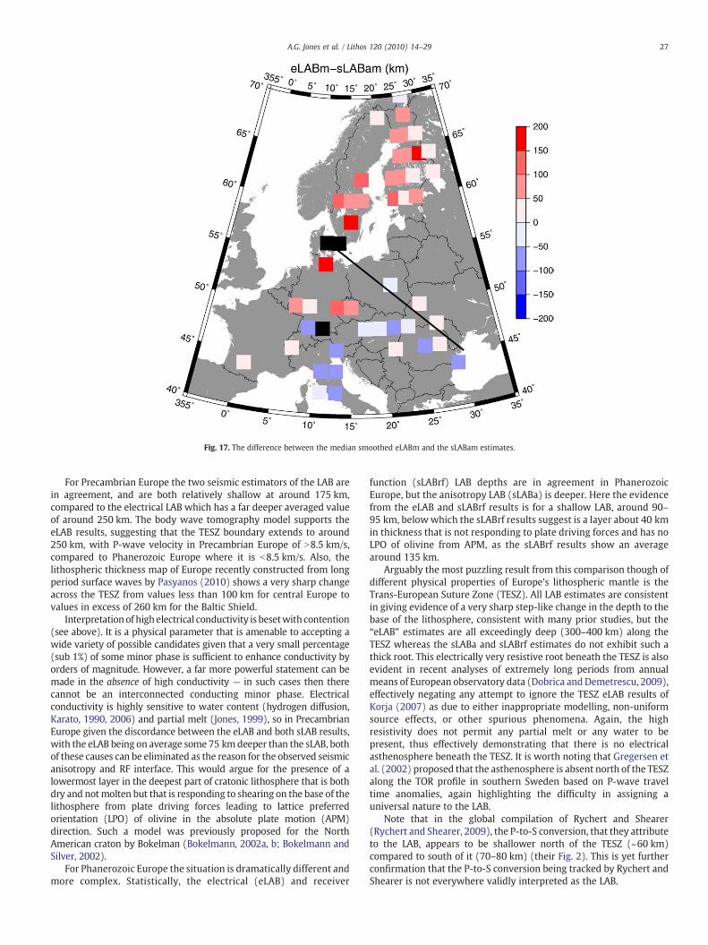
Fig. 17. The difference between the median smoothed eLABm and the sLABam estimates.

27A.G. Jones et al. / Lithos 120 (2010) 14–29

For Precambrian Europe the two seismic estimators of the LAB arein agreement, and are both relatively shallow at around 175 km,compared to the electrical LAB which has a far deeper averaged valueof around 250 km. The body wave tomography model supports theeLAB results, suggesting that the TESZ boundary extends to around250 km, with P-wave velocity in Precambrian Europe of N8.5 km/s,compared to Phanerozoic Europe where it is b8.5 km/s. Also, thelithospheric thickness map of Europe recently constructed from longperiod surface waves by Pasyanos (2010) shows a very sharp changeacross the TESZ from values less than 100 km for central Europe tovalues in excess of 260 km for the Baltic Shield.

Interpretation of high electrical conductivity is besetwith contention(see above). It is a physical parameter that is amenable to accepting awide variety of possible candidates given that a very small percentage(sub 1%) of some minor phase is sufficient to enhance conductivity byorders of magnitude. However, a far more powerful statement can bemade in the absence of high conductivity — in such cases then therecannot be an interconnected conducting minor phase. Electricalconductivity is highly sensitive to water content (hydrogen diffusion,Karato, 1990, 2006) and partial melt (Jones, 1999), so in PrecambrianEurope given the discordance between the eLAB and both sLAB results,with the eLAB being on average some 75 km deeper than the sLAB, bothof these causes can be eliminated as the reason for the observed seismicanisotropy and RF interface. This would argue for the presence of alowermost layer in the deepest part of cratonic lithosphere that is bothdry and notmolten but that is responding to shearing on the base of thelithosphere from plate driving forces leading to lattice preferredorientation (LPO) of olivine in the absolute plate motion (APM)direction. Such a model was previously proposed for the NorthAmerican craton by Bokelman (Bokelmann, 2002a, b; Bokelmann andSilver, 2002).

For Phanerozoic Europe the situation is dramatically different andmore complex. Statistically, the electrical (eLAB) and receiver

function (sLABrf) LAB depths are in agreement in PhanerozoicEurope, but the anisotropy LAB (sLABa) is deeper. Here the evidencefrom the eLAB and sLABrf results is for a shallow LAB, around 90–95 km, belowwhich the sLABrf results suggest is a layer about 40 kmin thickness that is not responding to plate driving forces and has noLPO of olivine from APM, as the sLABrf results show an averagearound 135 km.

Arguably the most puzzling result from this comparison though ofdifferent physical properties of Europe's lithospheric mantle is theTrans-European Suture Zone (TESZ). All LAB estimates are consistentin giving evidence of a very sharp step-like change in the depth to thebase of the lithosphere, consistent with many prior studies, but the“eLAB” estimates are all exceedingly deep (300–400 km) along theTESZ whereas the sLABa and sLABrf estimates do not exhibit such athick root. This electrically very resistive root beneath the TESZ is alsoevident in recent analyses of extremely long periods from annualmeans of European observatory data (Dobrica and Demetrescu, 2009),effectively negating any attempt to ignore the TESZ eLAB results ofKorja (2007) as due to either inappropriate modelling, non-uniformsource effects, or other spurious phenomena. Again, the highresistivity does not permit any partial melt or any water to bepresent, thus effectively demonstrating that there is no electricalasthenosphere beneath the TESZ. It is worth noting that Gregersen etal. (2002) proposed that the asthenosphere is absent north of the TESZalong the TOR profile in southern Sweden based on P-wave traveltime anomalies, again highlighting the difficulty in assigning auniversal nature to the LAB.

Note that in the global compilation of Rychert and Shearer(Rychert and Shearer, 2009), the P-to-S conversion, that they attributeto the LAB, appears to be shallower north of the TESZ (~60 km)compared to south of it (70–80 km) (their Fig. 2). This is yet furtherconfirmation that the P-to-S conversion being tracked by Rychert andShearer is not everywhere validly interpreted as the LAB.

28 A.G. Jones et al. / Lithos 120 (2010) 14–29

5. Conclusions

All three techniques used for identifying the lithosphere-astheno-sphere boundary, namely magnetotellurics (eLAB) and receiverfunction and anisotropy seismological methods (sLABrf and sLABa),are qualitatively consistent, with thin lithosphere in PhanerozoicEurope and thick lithosphere in Precambrian Europe, with a sharpchange at the Trans-European Suture Zone. This overarching result issupported by a new body wave tomographic model of Spakman(unpubl.) and by a recent long period surface wave model (Pasyanos,2010).

The three differ though quantitatively, with the eLAB and sLABrf inagreement for central Phanerozoic Europe, and the sLABa and sLABrfin agreement for Precambrian Europe, but both being thinner than theeLAB and the LAB thickness from the recent surface wave model(Pasyanos, 2010). Where there are thick sedimentary basins, innorthern Germany and the Pannonian Basin, the two seismologicaldefinitions, sLABa and sLABrf, are in agreement, to within error(±10 km) of each other.

For Precambrian Europe with its thick lithosphere, the sLABa andsLABrf definitions may be not the base of the lithosphere, but to aboundary within the lower lithosphere that is responding to shearingon the base of the lithosphere from plate driving forces (Bokelmannand Silver, 2002).

These quantitative differences between the three types of LABestimates, though substantial in some regions, are not random. Theyeach reflect some aspect(s) of the physical transition from thelithosphere to the asthenosphere, which need not be the same fordifferent parameters, for the different age of the provinces, and of thesame intensity relative to other discontinuities in the upper mantle.Classifying the differences does not define which of the methods isbetter or best, but contributes to improving our understanding of thenature of the lithosphere–asthenosphere boundary, which methodsare suitable for detailed modelling of this most prominent transitionin the upper mantle in different regions and to the interdisciplinaryresearch of the “bottom” of the lithospheric plates and their structure.

What we have not addressed is the sharpness of the LAB. The SRFmodelling suggests that the LAB is sharper beneath Central Europethan beneath the Precambrian platform of Eastern Europe (Geissleret al., 2010). Clearly, more detailed and focussed comparisons need tobe made of the LAB and its sharpness across the whole of Europe andother locations where good seismological and electromagnetic dataexist.

Acknowledgments

This paper is a result of the invitation to present a review of theEuropean LAB at the 33rd International Geological Congress held inOslo in August, 2008, and the authors wish to thank Sue O'Reillyfor that invitation. The authors wish to thank the two reviewers,Prof. Marek Grad and an unknown reviewer, and Guest Editor SueO'Reilly for their suggested improvements to the original version ofthis paper — their work has improved the final version.

The work of JP was supported by grant No. IAA300120709 of theGrant Agency of the Czech Academy of Sciences.

References

Amaru, M.L., Spakman, W., Villasenor, A., Sandoval, S., Kissling, E., 2008. A new absolutearrival time data set for Europe. Geophysical Journal International 173 (2),465–472.

Anderson, D.L., 1995. Lithosphere, asthenosphere, and perisphere. Reviews ofGeophysics 33 (1), 125–149.

Artemieva, I.M., 2009. The continental lithosphere: reconciling thermal, seismic, andpetrologic data. Lithos 109 (1–2), 23–46.

Babuska, V., Plomerova, J., 1992. The lithosphere in central Europe — seismological andpetrological aspects. Tectonophysics 207 (1–2), 141–163.

Babuska, V., Plomerova, J., 2006. European mantle lithosphere assembled from rigidmicroplates with inherited seismic anisotropy. Physics of the Earth and PlanetaryInteriors 158 (2–4), 264–280.

Babuska, V., Montagner, J.P., Plomerova, J., Girardin, N., 1998. Age-dependent large-scale fabric of the mantle lithosphere as derived from surface-wave velocityanisotropy. Pure and Applied Geophysics 151 (2–4), 257–280.

Bokelmann, G.H.R., 2002a. Convection-driven motion of the north American craton:evidence from P-wave anisotropy. Geophysical Journal International 148 (2),278–287.

Bokelmann, G.H.R., 2002b. Which forces drive North America? Geology 30 (11),1027–1030.

Bokelmann, G.H.R., Silver, P.G., 2002. Shear stress at the base of shield lithosphere.Geophysical Research Letters 29 (23), 4.

Constable, S., 2006. SEO3: a new model of olivine electrical conductivity. GeophysicalJournal International 166 (1), 435–437.

Dobrica, V., Demetrescu, C., 2009. Large-scale European mantle electric structure asderived from ring current and geomagnetic observatory data, 11th IAGA ScientificAssembly Sopron, Hungary.

Eaton, D.W., Darbyshire, F., Evans, R.L., Grutter, H., Jones, A.G., Yuan, X.H., 2009. Theelusive lithosphere–asthenosphere boundary (LAB) beneath cratons. Lithos 109(1–2), 1–22.

Evans, R.L., Hirth, G., Baba, K., Forsyth, D., Chave, A., Mackie, R., 2005. Geophysicalevidence from the MELT area for compositional controls on oceanic plates. Nature437 (7056), 249–252.

Fasano, G., Vio, R., 1988. Fitting a straight line with errors on both coordinates.Newsletter of Working Group for Modern Astronomical Methodology 7, 2–7.

Fischer, K.M., Ford, H.A., Abt, D.L., Rychert, C.A., 2010. The lithosphere–asthenosphereboundary, annual review of Earth and Planetary Sciences. Annual Review of Earthand Planetary Sciences vol. 38, 551–575.

Geissler, W.H., Sodoudi, F., Kind, R., 2010. Thickness of the central and eastern Europeanlithosphere as seen by S receiver functions. Geophysical Journal International 181(604–634).

Ghods, A., Arkani-Hamed, J., 2000. Melt migration beneath mid-ocean ridges.Geophysical Journal International 140, 687–697.

Gregersen, S., Voss, P., Grp, T.O.R.W., 2002. Summary of project TOR: delineation of astepwise, sharp, deep lithosphere transition across Germany–Denmark–Sweden.Tectonophysics 360 (1–4), 61–73.

Guterch, A., Grad, M., 2006. Lithospheric structure of the TESZ in Poland based onmodern seismic experiments. Geological Quarterly 50 (1), 23–32.

Hales, A.L., 1969. A seismic discontinuity in the lithosphere. Earth and Planetary ScienceLetters 7, 44–46.

Hartigan, P.M., 1985. Algorithm AS217: computation of the dip statistic to test forunimodality. Applied Statistics 34 (3), 320–325.

Hartigan, J.A., Hartigan, P.M., 1985. The dip test of unimodality. The Annals of Statistics13 (1), 70–84.

Heinson, G., 1999. Electromagnetic studies of the lithosphere and asthenosphere.Surveys in Geophysics 20 (3–4), 229–255.

Heit, B., Sodoudi, F., Yuan, X., Bianchi, M., Kind, R., 2007. An S receiver function analysisof the lithospheric structure in South America. Geophysical Research Letters 34(14).

Hirth, G., Evans, R.L., Chave, A.D., 2000. Comparison of continental and oceanic mantleelectrical conductivity: is the archean lithosphere dry. Geochemistry, Geophysics,Geosystems 1.

Huber, P.J., 1981. Robust Statistics. John Wiley, New York. 308 pp.Jones, A.G., 1980. Geomagnetic induction studies in Scandinavia—I. Determination of

the inductive response function from the magnetometer data. Journal ofGeophysics 48, 181–194 (Zeitschrift fuer Geophysik).

Jones, A.G., 1988. Static shift of magnetotelluric data and its removal in a sedimentarybasin environment. Geophysics 53 (7), 967–978.

Jones, A.G., 1999. Imaging the continental upper mantle using electromagneticmethods. Lithos 48 (1–4), 57–80.

Jones, A.G., Spratt, J., 2002. A simplemethod for deriving the uniform fieldMT responsesin auroral zones. Earth Planets and Space 54 (5), 443–450.

Jones, A.G., Evans, R.L., Eaton, D.W., 2009. Velocity–conductivity relationships formantle mineral assemblages in Archean cratonic lithosphere based on a review oflaboratory data and application of extremal bound theory. Lithos 109, 131–143.

Karato, S., 1990. The role of hydrogen in the electrical conductivity of the upper mantle.Nature 347 (6290), 272–273.

Karato, S., 2006. Remote sensing of hydrogen in Earth's mantle, Water in NominallyAnhydrous Minerals. Reviews in Mineralogy & Geochemistry. Mineralogical SocAmerica, Chantilly, pp. 343–375.

Kawakatsu, H., Kumar, P., Takei, Y., Shinohara, M., Kanazawa, T., Araki, E., Suyehiro, K.,2009. Seismic evidence for sharp lithosphere–asthenosphere boundaries of oceanicplates. Science 324 (5926), 499–502.

Kennedy, C.S., Kennedy, G.C., 1976. Equilibrium boundary between graphite anddiamond. Journal of Geophysical Research, Solid Earth 81 (14), 2467–2470.

Kennett, B.L.N., Engdahl, E.R., Buland, R., 1995. Constraints on seismic velocities in theEarth from travel times. Geophysical Journal of the Royal Astronomical Society 122,108–124.

Korja, T., 2007. How is the european lithosphere imaged by magnetotellurics? Surveysin Geophysics 28 (2–3), 239–272.

Kumar, P., Kind, R., Hanka, W., Wylegalla, K., Reigber, C., Yuan, X., Woelbern, I.,Schwintzer, P., Fleming, K., Dahl-Jensen, T., Larsen, T.B., Schweitzer, J., Priestley, K.,Gudmundsson, O., Wolf, D., 2005. The lithosphere–asthenosphere boundary in theNorth-West Atlantic region. Earth and Planetary Science Letters 236 (1–2),249–257.

29A.G. Jones et al. / Lithos 120 (2010) 14–29

Lahti, I., Korja, T., Kaikkonen, P., Vaittinen, K., Grp, B.W., 2005. Decomposition analysis ofthe BEAR magnetotelluric data: implications for the upper mantle conductivity inthe Fennoscandian Shield. Geophysical Journal International 163 (3), 900–914.

Ledo, J., Jones, A.G., 2005. Upper mantle temperature determined from combiningmineral composition, electrical conductivity laboratory studies and magnetotellu-ric field observations: application to the Intermontane belt, Northern CanadianCordillera. Earth and Planetary Science Letters 236 (1–2), 258–268.

Li, X.Q., Yuan, X.H., Kind, R., 2007. The lithosphere–asthenosphere boundary beneaththe western United States. Geophysical Journal International 170 (2), 700–710.

Maumus, J., Bagdassarov, N., Schmeling, H., 2005. Electrical conductivity and partialmelting of mafic rocks under pressure. Geochimica Et Cosmochimica Acta 69 (19),4703–4718.

Partzsch, G.M., Schilling, F.R., Arndt, J., 2000. The influence of partial melting on theelectrical behavior of crustal rocks: laboratory examinations, model calculationsand geological interpretations. Tectonophysics 317 (3–4), 189–203.

Pasyanos, M.E., 2010. Lithospheric thickness modeled from long-period surface wavedispersion. Tectonophysics 481 (1–4), 38–50.

Plomerova, J., Babuska, V., 2010. Long memory of mantle lithosphere fabric— EuropeanLAB constrained from seismic anisotropy. Lithos. doi:10.1016/j.lithos.2010.01.008.

Plomerova, J., Babuska, V., Vecsey, L., Kouba, D., Grp, T.O.R.W., 2002a. Seismic anisotropy ofthe lithosphere around the Trans-European Suture Zone (TESZ) based on teleseismicbody-wave data of the TOR experiment. Tectonophysics 360 (1–4), 89–114.

Plomerova, J., Kouba, D., Babuska, V., 2002b. Mapping the lithosphere-asthenosphereboundary through changes in surface-wave anisotropy. Tectonophysics 358 (1–4),175–185.

Plomerova, J., Babuska, V., Vecsey, L., Kozlovskaya, E., Raita, T., Sstwg, 2006.Proterozoic–Archean boundary in the mantle lithosphere of eastern Fennoscandiaas seen by seismic anisotropy. Journal of Geodynamics 41 (4), 400–410.

Plomerova, J., Babuska, V., Kozovskaya, E., Vecsey, L., Hyvonen, L.T., 2008. Seismicanisotropy — a key to resolve fabrics of mantle lithosphere of Fennoscandia.Tectonophysics 462 (1–4), 125–136.

Praus, O., Pecova, J., Petr, V., Babuska, V., Plomerova, J., 1990. Magnetotelluric andseismological determination of the lithosphere–asthenosphere transition incentral-Europe. Physics of the Earth and Planetary Interiors 60 (1–3), 212–228.

Pushkarev, P.Y., Ernst, T., Jankowski, J., Jozwiak, W., Lewandowski, M., Nowozynski, K.,Semenov, V.Y., 2007. Deep resistivity structure of the Trans-European Suture Zonein central Poland. Geophysical Journal International 169 (3), 926–940.

Revenaugh, J., Jordan, T.H., 1991. Mantle layering from ScS reverberations: 3. The uppermantle. Journal of Geophysical Research 96 (B12), 19,781–19,810.

Romanowicz, B., 2009. The thickness of tectonic plates. Science 324 (5926), 474–476.

Rychert, C.A., Shearer, P.M., 2009. A global view of the lithosphere–asthenosphereboundary. Science 324 (5926), 495–498.

Rychert, C.A., Shearer, P.M., Fischer, K.M., 2010. Scattered wave imaging of thelithosphere–asthenosphere boundary. Lithos 120, 173–185.

Semenov, V.Y., Pek, J., Adam, A., Jozwiak, W., Ladanyvskyy, B., Logvinov, I.M., Pushkarev,P., Vozar, J., 2008. Electrical structure of the upper mantle beneath Central Europe:results of the CEMES project. Acta Geophysica 56 (4), 957–981.

Smirnov, M.Y., Pedersen, L.B., 2009. Magnetotelluric measurements across theSorgenfrei–Tornquist Zone in southern Sweden and Denmark. Geophysical JournalInternational 176 (2), 443–456.

Sodoudi, F., Yuan, X., Liu, Q., Kind, R., Chen, J., 2006a. Lithospheric thickness beneath theDabie Shan, central eastern China from S receiver functions. Geophysical JournalInternational 166 (3), 1363–1367.

Sodoudi, F., Kind, R., Hatzfeld, D., Priestley, K., Hanka, W., Wylegalla, K., Stavrakakis, G.,Vafidis, A., Harjes, H.P., Bohnhoff, M., 2006b. Lithospheric structure of the Aegeanobtained from P and S receiver functions. Journal of Geophysical Research, SolidEarth 111 (B12).

Sodoudi, F., Yuan, X., Kind, R., Heit, B., Sadidkhouy, A., 2009. Evidence for a missingcrustal root and a thin lithosphere beneath the Central Alborz by receiver functionstudies. Geophysical Journal International 177, 733–742.

Tirone, M., Ganguly, J., Morgan, J.P., 2009. Modeling petrological geodynamics in theEarth's mantle. Geochemistry, Geophysics, Geosystems 10 (4), 28.

Varentsov, I.M., Sokolova, E.Y., Grp, B.W., 2003. Diagnostics and suppression of auroraldistortions in the transfer operators of the electromagnetic field in the BEARexperiment. Izvestiya Physics of the Solid Earth 39 (4), 283–307.

Velikhov, Y.P., Zhamaletdinov, A.A., Belkov, I.V., Gorbunov, G.I., Hjelt, S.E., Lisin, A.S.,Vanyan, L.L., Zhdanov, M.S., Demidova, T.A., Korja, T., Kirillov, S.K., Kuksa, Y.I.,Poltanov, A.Y., Tokarev, A.D., Yevstigneyev, V.V., 1986. Electromagnetic studies onthe Kola Peninsula and in Northern Finland by means of a powerful controlledsource. Journal of Geodynamics 5, 237–256.

Wilde-Piorko, M., Swieczak, M., Grad, M., Majdanski, M., 2010. Integrated seismicmodel of the crust and upper mantle of the Trans-European Suture zone betweenthe Precambrian craton and Phanerozoic terranes in Central Europe. Tectonophy-sics 481 (1–4), 108–115.

York, D., 1966. Least-squares fitting of a straight line. Canadian Journal of Physics 44 (5),1079–1086.

York, D., 1969. Least squares fitting of a straight line with correlated errors. Earth andPlanetary Science Letters 5, 320–324.

Yuan, X.H., Kind, R., Li, X.Q., Wang, R.J., 2006. The S receiver functions: synthetics anddata example. Geophysical Journal International 165 (2), 555–564.