Lithosphere of the Dharwar craton by joint inversion of P and S receiver functions

Geophys. J. Int. (2008) 173, 1106–1118 doi: 10.1111/j.1365-246X.2008.03777.xG

JITec

toni

csan

dge

ody

nam

ics

Lithosphere of the Dharwar craton by joint inversion of P and Sreceiver functions

S. Kiselev,1 L. Vinnik,1 S. Oreshin,1 S. Gupta,2 S. S. Rai,2 A. Singh,2 M. R. Kumar2

and G. Mohan3

1Institute of Physics of the Earth, B. Grouzinskaya 10, 123995 Moscow, Russia. E-mail: [email protected] Geophysical Research Institute, Hyderabad-500 007, India3Department of Earth Sciences, Indian Institute of Technology, Powai, Mumbai 400076, India

Accepted 2008 March 2. Received 2008 February 18; in original form 2007 March 22

S U M M A R YThe Archean Dharwar craton in south India is known for long time to be different from mostother cratons. Specifically, at station Hyderabad (HYB) the Ps converted phases from the 410-and 660-km mantle discontinuities arrive up to 2 s later than in other cratons of comparable age,which implies lower upper mantle velocities. To resolve the unique lithosphere–asthenospheresystem of the Dharwar craton, we inverted jointly P and S receiver functions and teleseismic Pand S traveltime residuals at 10 seismograph stations. This method operates in the same depthrange as long-period surface waves but differs by much higher lateral and radial resolution.We observe striking differences in crustal structures between the eastern and western Dharwarcraton (EDC and WDC, respectively): crustal thickness is of around 31 km, with predominantlyfelsic velocities, in the EDC and of around 55 km, with predominantly mafic velocities, in theWDC. In the mantle we observe significant variations in the P velocity with depth, practicallywithout accompanying variations in the S velocity. In the mantle S velocity there are azimuth-dependent indications of the Hales discontinuity at a depth of ∼100 km. The most conspicuousfeature of our models is the lack of the high velocity mantle keel with the S velocity of∼4.7 km s−1, typical of other Archean cratons. The S velocity in our models is close to4.5 km s−1 from the Moho to a depth of ∼250 km. There are indications of a similar uppermantle structure in the northeast of the Indian craton and of a partial recovery of the normalshield structure in the northwest. A division between the high S-velocity western Tibet andlow S-velocity eastern Tibet may be related to a similar division between the northeastern andnorthwestern Indian craton.

Key words: Composition of the mantle; Body waves; Wave propagation; Cratons; Crustalstructure; Asia.

1 I N T RO D U C T I O N

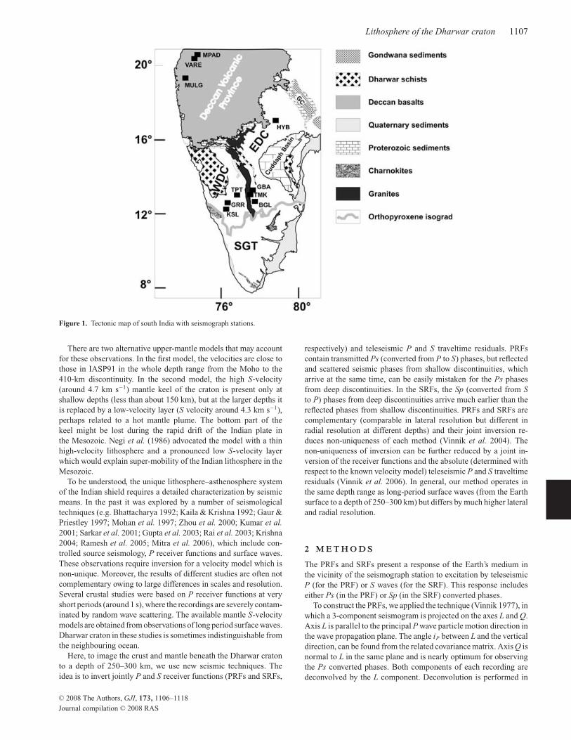
The Indian craton is amalgamation of a few smaller cratons (Drury

et al. 1984; Taylor et al. 1984). Its southern part is occupied by the

Dharwar craton (Fig. 1). The mid-Archean greenstone belt in the

western Dharwar craton (WDC) presents one of the oldest cratonic

nuclei (Raase et al. 1986). Evolution of the greenstone belt is a

consequence of volcanism around 3.6 Gyr ago and stabilization at

2.7 Gyr. In the north, the WDC is covered by 65 Myr old Deccan

traps (DVP, Deccan Volcanic Province). The late Archean granite–

gneiss terrain of the eastern Dharwar craton (EDC) was formed at

2.5 Gyr and stabilized in early Proterozoic. The southernmost Dhar-

war craton is occupied by the Southern Granulite Terrain (SGT).

The Dharwar craton differs in the properties of the upper man-

tle from most other cratons of comparable age. The difference is

suggested by the observations of the P-to-S (Ps) converted phases

from the discontinuities bounding the mantle transition zone (TZ)

at around 410–660 km depths. Topography on the discontinuities

can be significant in anomalously hot and cold regions of the TZ—

hotspots and subduction zones, respectively—but in other regions

the arrival times of the Ps converted phases are controlled mainly

by the wave velocities in the crust and mantle over the 410 km

discontinuity (Chevrot et al. 1999). We use IASP91 standard earth

model (Kennett & Engdahl 1991) as a reference. At seismograph

stations in the Archean cratons (Canadian, Siberian, East-European,

Kalahari in southern Africa and some others), the Ps converted

phases from the TZ discontinuities arrive up to 2 s earlier than

in IASP91 (Chevrot et al. 1999); early arrivals are caused by the

high S velocities in the roots of the cratons, extending to a depth

of about 250 km. However, the arrivals of P410s and P660s at seis-

mograph station Hyderabad (HYB) in south India (Fig. 1) are ob-

served practically at the standard time (Chevrot et al. 1999). A

similar time is observed at stations in the DVP (Kumar & Mohan

2005).

1106 C© 2008 The Authors

Journal compilation C© 2008 RAS

Lithosphere of the Dharwar craton 1107

Figure 1. Tectonic map of south India with seismograph stations.

There are two alternative upper-mantle models that may account

for these observations. In the first model, the velocities are close to

those in IASP91 in the whole depth range from the Moho to the

410-km discontinuity. In the second model, the high S-velocity

(around 4.7 km s−1) mantle keel of the craton is present only at

shallow depths (less than about 150 km), but at the larger depths it

is replaced by a low-velocity layer (S velocity around 4.3 km s−1),

perhaps related to a hot mantle plume. The bottom part of the

keel might be lost during the rapid drift of the Indian plate in

the Mesozoic. Negi et al. (1986) advocated the model with a thin

high-velocity lithosphere and a pronounced low S-velocity layer

which would explain super-mobility of the Indian lithosphere in the

Mesozoic.

To be understood, the unique lithosphere–asthenosphere system

of the Indian shield requires a detailed characterization by seismic

means. In the past it was explored by a number of seismological

techniques (e.g. Bhattacharya 1992; Kaila & Krishna 1992; Gaur &

Priestley 1997; Mohan et al. 1997; Zhou et al. 2000; Kumar et al.2001; Sarkar et al. 2001; Gupta et al. 2003; Rai et al. 2003; Krishna

2004; Ramesh et al. 2005; Mitra et al. 2006), which include con-

trolled source seismology, P receiver functions and surface waves.

These observations require inversion for a velocity model which is

non-unique. Moreover, the results of different studies are often not

complementary owing to large differences in scales and resolution.

Several crustal studies were based on P receiver functions at very

short periods (around 1 s), where the recordings are severely contam-

inated by random wave scattering. The available mantle S-velocity

models are obtained from observations of long period surface waves.

Dharwar craton in these studies is sometimes indistinguishable from

the neighbouring ocean.

Here, to image the crust and mantle beneath the Dharwar craton

to a depth of 250–300 km, we use new seismic techniques. The

idea is to invert jointly P and S receiver functions (PRFs and SRFs,

respectively) and teleseismic P and S traveltime residuals. PRFs

contain transmitted Ps (converted from P to S) phases, but reflected

and scattered seismic phases from shallow discontinuities, which

arrive at the same time, can be easily mistaken for the Ps phases

from deep discontinuities. In the SRFs, the Sp (converted from Sto P) phases from deep discontinuities arrive much earlier than the

reflected phases from shallow discontinuities. PRFs and SRFs are

complementary (comparable in lateral resolution but different in

radial resolution at different depths) and their joint inversion re-

duces non-uniqueness of each method (Vinnik et al. 2004). The

non-uniqueness of inversion can be further reduced by a joint in-

version of the receiver functions and the absolute (determined with

respect to the known velocity model) teleseismic P and S traveltime

residuals (Vinnik et al. 2006). In general, our method operates in

the same depth range as long-period surface waves (from the Earth

surface to a depth of 250–300 km) but differs by much higher lateral

and radial resolution.

2 M E T H O D S

The PRFs and SRFs present a response of the Earth’s medium in

the vicinity of the seismograph station to excitation by teleseismic

P (for the PRF) or S waves (for the SRF). This response includes

either Ps (in the PRF) or Sp (in the SRF) converted phases.

To construct the PRFs, we applied the technique (Vinnik 1977), in

which a 3-component seismogram is projected on the axes L and Q.

Axis L is parallel to the principal P wave particle motion direction in

the wave propagation plane. The angle iP between L and the vertical

direction, can be found from the related covariance matrix. Axis Q is

normal to L in the same plane and is nearly optimum for observing

the Ps converted phases. Both components of each recording are

deconvolved by the L component. Deconvolution is performed in

C© 2008 The Authors, GJI, 173, 1106–1118


1108 S. Kiselev et al.

time domain (Berkhout 1977) with a proper regularization (damping

parameter is equal to 3.0).

To detect the Ps phases from deep discontinuities, the individual

Q components are stacked with move-out time corrections. Like

in Vinnik (1977) and other similar studies, the adopted reference

slowness is 6.4 s/◦ (seconds per degree). The result of stacking is

presented as a set of traces for different trial conversion depths. The

depth of the discontinuity can be found accurately from the arrival

time of the Ps converted phase, or it can be evaluated tentatively as

a trial conversion depth corresponding to the largest amplitude of

this phase. A compatibility of both estimates implies that an arrival

is identified correctly as the Ps phase.

Calculation of the SRF (Farra & Vinnik 2000) involves seismo-

gram decomposition into Q, L, T and M components. The Q and Lcomponents here are different from those in the PRFs. Q corresponds

to the principal S particle motion direction in the wave propagation

plane. Angle iSV between the Q axis and the radial direction is de-

termined from the related covariance matrix. L is perpendicular to

Q in the same plane and is nearly optimum for detecting the Spconverted phases. T is perpendicular to the wave propagation plane,

and M is the principal S particle motion component in the plane

containing the Q and T components. The angle θ between the axes

Q and M is controlled by the focal mechanism of the earthquake.

All components are deconvolved by the M component.

The Sp converted phases can be generated by the SV and SH (in

the case of azimuthal anisotropy) components of the incoming Swave. To isolate the Sp phases generated by SV , the individual re-

ceiver functions of many events are stacked with weights depending

on θ and the level of noise. The result of stacking is the L component

deconvolved by the Q component of the S wave and normalized to

the amplitude of the Q component. The procedure involves eval-

uation of σ , the rms value of noise in the stack. To account for

the difference in slowness between the S and Sp phases from deep

discontinuities, the individual receiver functions are stacked with

time corrections (slant stacking). The correction is calculated as the

product of the trial differential slowness and the differential epi-

central distance (difference between the epicentral distance of the

seismic event and the reference epicentral distance of the group of

events). The stack is calculated for a number of values of the dif-

ferential slowness. The move-out corrections for different depths

of conversion can be calculated more accurately, but at the rela-

tively long periods of the SRFs (around 10 s) and in the narrow

range of the S wave slowness (between 12.3 s (◦)−1 at a distance

of 65◦ and 9.2 s (◦)−1 at a distance of 90◦) the gain in accuracy is

negligible.

The SRF technique is most efficient in the distance range between

65◦ and 90◦. In the distance range between 75◦ and 90◦, SKS seismic

phase arrives within 30 s of S, and at around 83◦, they even arrive

at the same time. How the potential interference between S and SKSaffects performance of the SRF technique? The Sp and SKSp con-

verted phases from discontinuities at depths less than 100 km arrive

with a negligible difference in time (small relative to the dominant

period of 10 s), but at larger depth the difference becomes signifi-

cant, around 10 s for a depth of 400 km. The 410-km discontinuity

is global, and the converted phases from this discontinuity are of

great diagnostic value. Numerical simulations reveal three possi-

ble kinds of interaction between S and SKS in S receiver functions:

(1) contribution of SKS to the wave train used is small relative to S;

(2) contribution of S is small relative to SKS and (3) contributions

of S and SKS are comparable. In the first case, the detected signal is

S410p, in the 2nd case this is SKS410p. In the 3rd case, no signal is

detected because the waveform used for deconvolution is strongly

different from both S and SKS. We will show that in most of our

receiver functions, the detected signal is S410p with implication that

the S wave is dominant and the effect of interference between S and

SKS is small.

Constraining the models by the teleseismic traveltime residuals

(Vinnik et al. 2006) is based on the fact that the major mantle dis-

continuities are related to the phase transitions, the depths of which

depend on the temperature. Outside the anomalously hot and cold

regions (hotspots and subduction zones, respectively), the difference

between the arrival times of the P660s and P410s phases (23.9 s) is

stable, with implications that the discontinuities are located virtually

at the same depths (Chevrot et al. 1999). Then the lateral variations

of times of these phases are controlled by the P and S velocities

at depths less than 410 km. The arrival time of the Ps converted

phase is measured relative to the P wave. Therefore, the anomaly

of the arrival time of the Ps phase dTPs can be presented as dTPs =dTS − dTP, where dTS and dTP are the absolute teleseismic travel-

time residuals of the S and P waves, respectively. Following Vinnik

et al. (1999) this relation can be written as dTP = dTPs/(k − 1);

dTS = dTPs [1 + 1/(k − 1)], where k is the ratio between the S and

P residuals. For the same length of the wave path for the P and Swaves, and assuming that the velocity variations are caused by the

temperature, k = 2.7 (Vinnik et al. 1999). In the PRFs, the wave

path of the S wave is shorter than of the P wave by ∼ 10 per cent.

With the correction for the difference in lengths of the wave paths,

k = 2.4. We assume, in agreement with numerous studies (e.g. Grand

2002), that the largest lateral P and S velocity variations are in the

upper 250–300 km of the Earth, in the layer sampled by the receiver

functions. Then the P and S residuals thus obtained, dTP and dTS can

be used to constrain the velocity profiles inferred from the receiver

functions.

Our technology of inversion of the receiver functions was previ-

ously described by Vinnik et al. (2006, 2007). Nevertheless, for the

convenience of the reader we describe it again. We assume that the

Earth in the vicinity of the station is homogeneous and isotropic.

As a rule, we use the 0 km trace of the PRFs and 0 s/◦ trace of

SRFs. Other traces could be more appropriate for depths around

200 km, but at the relatively long periods of our receiver functions

this effect is negligible. The model is defined by the P and S veloc-

ities VP and VS , density and thickness of each plane layer. Density

is derived from the P velocity by using Birch law. For the PRFs

and SRFs we calculate synthetic Q and L components, respectively,

as:

Q P,syn(t, m, cp) = 1

2π

∫ +∞

−∞

HP,Q(ω, m, cp)

HP,L (ω, m, cp)

× L P,obs(ω) exp(iωt) dω, (1)

L SV,syn(t, m, cs) = 1

2π

∫ +∞

−∞

HSV,L (ω, m, cs)

HSV,Q(ω, m, cs)

× QSV,obs(ω) exp(iωt) dω. (2)

Here t is time, ω is angular frequency, m is the vector of unknown

model parameters, cP and cS are the adopted apparent velocities for

the PRFs and SRFs, respectively, indices ‘obs’ and ‘syn’ corre-

spond to the actual receiver functions and their synthetic analogues,

respectively, and H are theoretical transfer functions for the stack

of plane layers. Angles iP and iSV are known for each individual

receiver function but not for the stacked ones. Also, sometimes the

calculated receiver functions are later additionally filtered without

changing the angles iP and iSV . Therefore, in the inversion these

angles are included in m and allowed to vary within a few degrees

C© 2008 The Authors, GJI, 173, 1106–1118



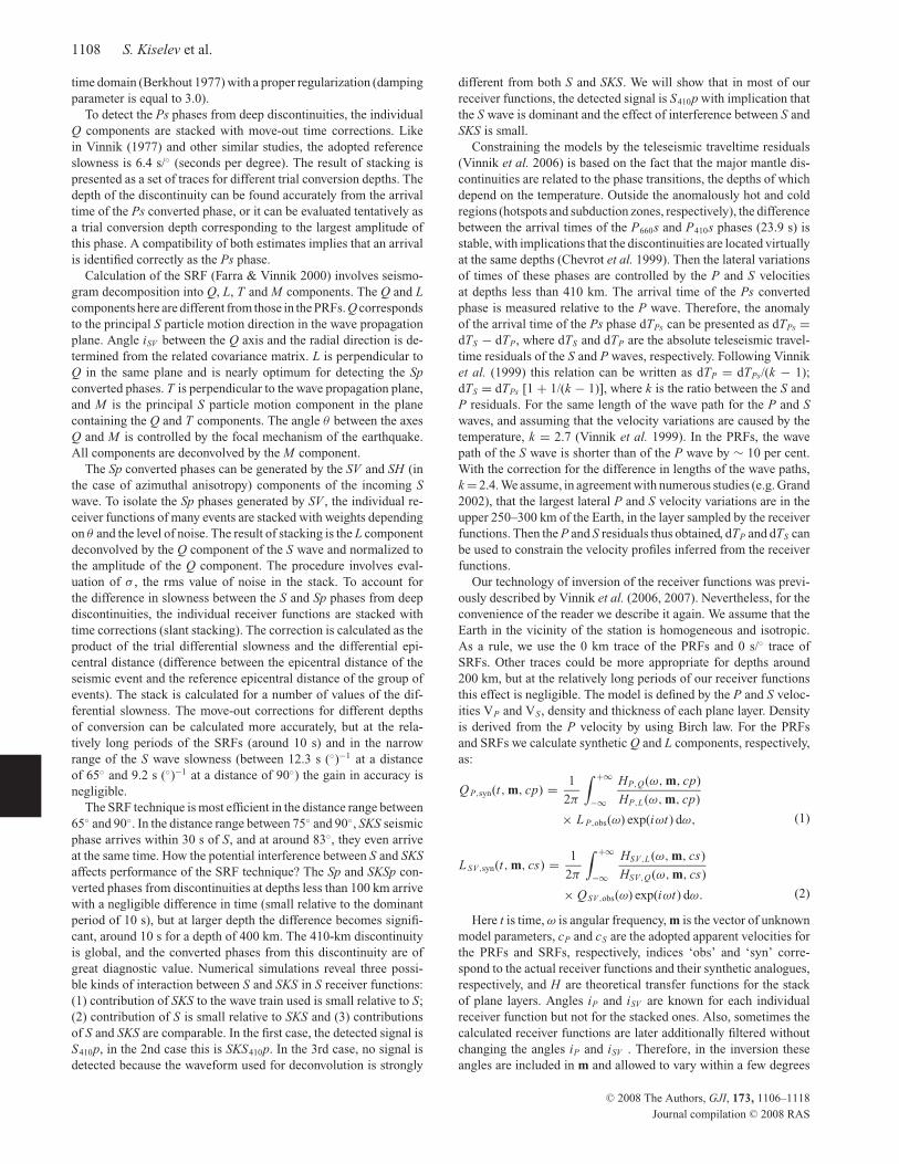
Figure 2. Histograms of the S velocity (colour code) obtained by inversion of the PRFs (a), SRFs (b), PRFs and SRFs (c), PRFs, SRFs and the P and Straveltime residuals (d) from station CHAT in the Tien Shan (modified from Vinnik et al. 2006). IASP91 velocities and medians are shown by bold and dash

lines, respectively. The related synthetic Q components of the PRFs and the L components of the SRFs are shown with the same colour code; the actual

components are shown by dash lines.

of their respective average values. The values of cP and cS are fixed

at the average values of apparent velocities for the P and S waves,

respectively. The synthetic receiver functions are calculated with

the aid of Thomson–Haskell matrix algorithm (Haskell 1962). Earth

flattening transformation is applied as in Biswas (1972).

Let EP (m) and ES (m) be misfits for the stacked Q components

of the PRFs and L components of the SRFs, respectively. The misfit

(cost) is defined as the rms difference between the observed and

synthetic functions. The inversion is then to manipulate m to min-

imize EP (m) and ES (m) simultaneously. We conduct a search for

the optimum models by using an interactive algorithm, similar to

Simulated Annealing (Mosegaard & Vestergaard 1991): the cost

functions are minimized by applying a set of moves, that is, a set

of model perturbations, and accepting or rejecting the moves ac-

cording to the Metropolis rule (Metropolis et al. 1953). For the two

cost functions we use the Metropolis rule in cascade (Mosegaard &

Tarantola 1995).

The Metropolis rule is formulated by using a parameter termed

temperature. We use step-wise temperature function. The value of

temperature at each step is chosen by the condition that the search,

when initialized at an arbitrary point m0 within chosen bounds,

converges to the same point for any m0. The inversion procedure

may require several temperature iterations. For a new iteration we

set narrowed bounds resulting from the previous iteration, and re-

peat manual adjustment of temperature. The procedure is terminated

when the cost function in the convergence point has reached suf-

ficiently small pre-defined level, usually around 0.02. To visualize

the results of the inversion we divide the parameter space into cells,

and present the models by the number of hits in each cell, and show

this number by the colour code. A similar statistics is demonstrated

for the data space.

The technique for the joint inversion of the PRF and SRF (using

the Metropolis rule in cascade for the two functions) can be easily

extended for the joint inversion of the receiver functions and the

traveltime residuals. The traveltime residuals for the trial models

are evaluated by ray tracing in the spherical Earth for the average

apparent velocities of the P receiver functions.

Advantages of the joint inversion are illustrated by the data from

station CHAT in the Tien Shan (Fig. 2, modified from Vinnik et al.2006) and from station HYB of the present study (Fig. 3). For each

station, we show the histograms of the S velocity obtained by the

inversion of only the PRF (a), only the SRF (b), both PRF and

SRF (c), and PRF, SRF and the traveltime residuals (d). We also

show the histograms of the related synthetic PRFs and SRFs. At

station CHAT, the models in (a) are not optimal for the SRF; this

is expressed in a large scatter of the synthetic SRFs. Similarly, the

models in (b) are not optimal for the PRFs. The joint inversion (c)

yields the models that are optimal for both the PRF and the SRF.

Finally, the histogram of the S velocity from the PRF, SRF and the

traveltime residuals (d) is more narrow than the others, and some

details of the models are more clear—a high velocity mantle lid and

the underlying LVZ with a boundary between them at a depth around

100 km. The LVZ is terminated at a depth of 200–230 km (the

Lehmann discontinuity).

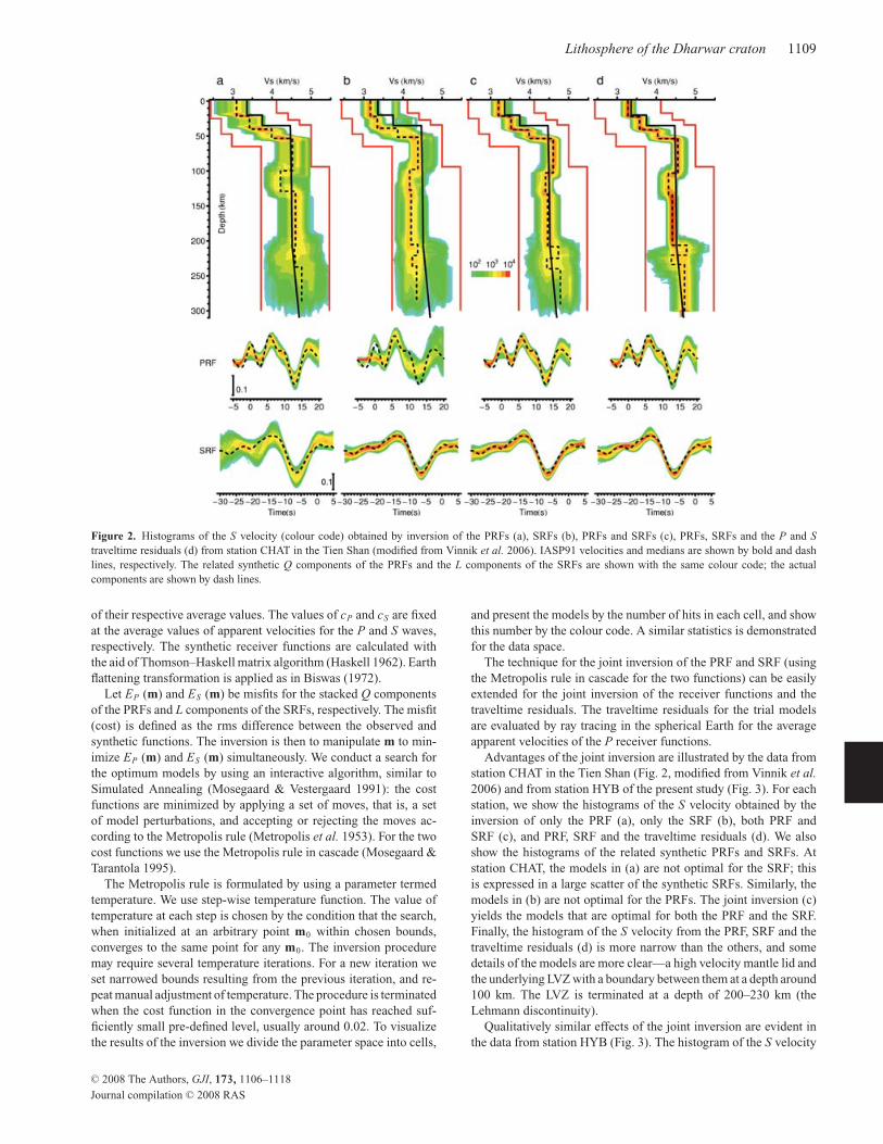
Qualitatively similar effects of the joint inversion are evident in

the data from station HYB (Fig. 3). The histogram of the S velocity

C© 2008 The Authors, GJI, 173, 1106–1118



Figure 3. The same as Fig. 2, but from station HYB of the present study.

in (d) is very narrow and reveals a weak but distinct positive discon-

tinuity (with a higher velocity at the lower side) at a depth around

80 km. The crustal histogram is narrow in (d) relative to (c) in spite

of the fact that the traveltime residuals are accumulated mainly in

the mantle. However, the model velocities in the crust and the man-

tle depend on each other via the receiver functions and constraining

the velocities in the mantle affects those in the crust.

In the last years, the SRF techniques were practiced by several

groups of researchers (e.g. Angus et al. 2006; Wilson et al. 2006).

The most important distinctions of our methodology are, first, the

rigorous inversion technique, and second, the joint inversion of the

SRFs, PRFs and the traveltime residuals. In most studies, the SRFs

are transformed into the velocity models semi-intuitively, and the

positive bump between −10 and −20 s in Figs 2 and 3 is interpreted

as the Sp phase from the ’LAB’, the boundary between the high

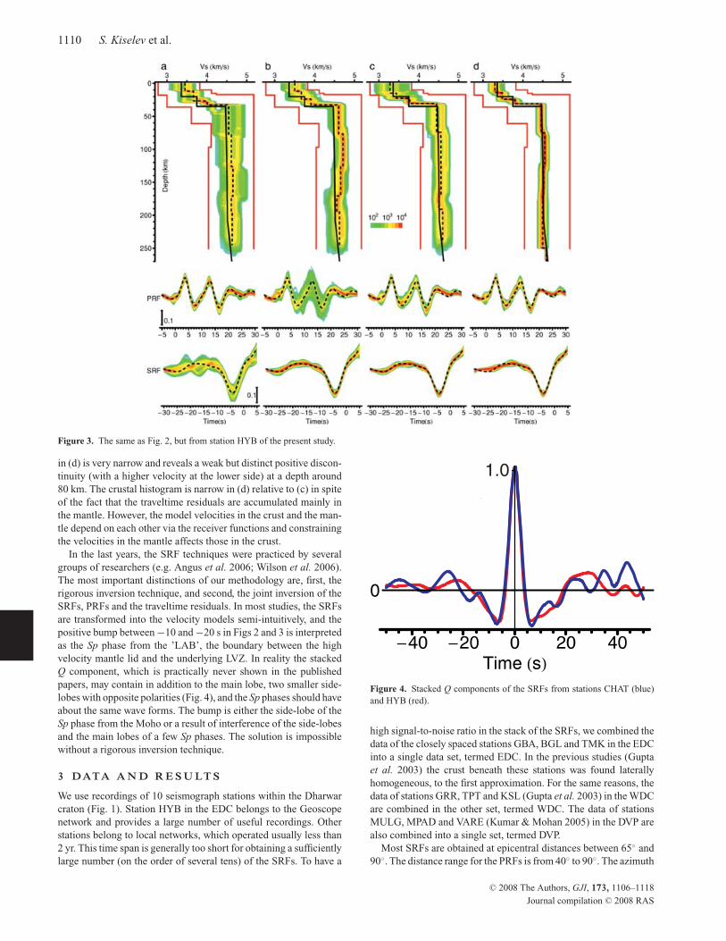
velocity mantle lid and the underlying LVZ. In reality the stacked

Q component, which is practically never shown in the published

papers, may contain in addition to the main lobe, two smaller side-

lobes with opposite polarities (Fig. 4), and the Sp phases should have

about the same wave forms. The bump is either the side-lobe of the

Sp phase from the Moho or a result of interference of the side-lobes

and the main lobes of a few Sp phases. The solution is impossible

without a rigorous inversion technique.

3 DATA A N D R E S U LT S

We use recordings of 10 seismograph stations within the Dharwar

craton (Fig. 1). Station HYB in the EDC belongs to the Geoscope

network and provides a large number of useful recordings. Other

stations belong to local networks, which operated usually less than

2 yr. This time span is generally too short for obtaining a sufficiently

large number (on the order of several tens) of the SRFs. To have a

.

1.0

Figure 4. Stacked Q components of the SRFs from stations CHAT (blue)

and HYB (red).

high signal-to-noise ratio in the stack of the SRFs, we combined the

data of the closely spaced stations GBA, BGL and TMK in the EDC

into a single data set, termed EDC. In the previous studies (Gupta

et al. 2003) the crust beneath these stations was found laterally

homogeneous, to the first approximation. For the same reasons, the

data of stations GRR, TPT and KSL (Gupta et al. 2003) in the WDC

are combined in the other set, termed WDC. The data of stations

MULG, MPAD and VARE (Kumar & Mohan 2005) in the DVP are

also combined into a single set, termed DVP.

Most SRFs are obtained at epicentral distances between 65◦ and

90◦. The distance range for the PRFs is from 40◦ to 90◦. The azimuth

C© 2008 The Authors, GJI, 173, 1106–1118



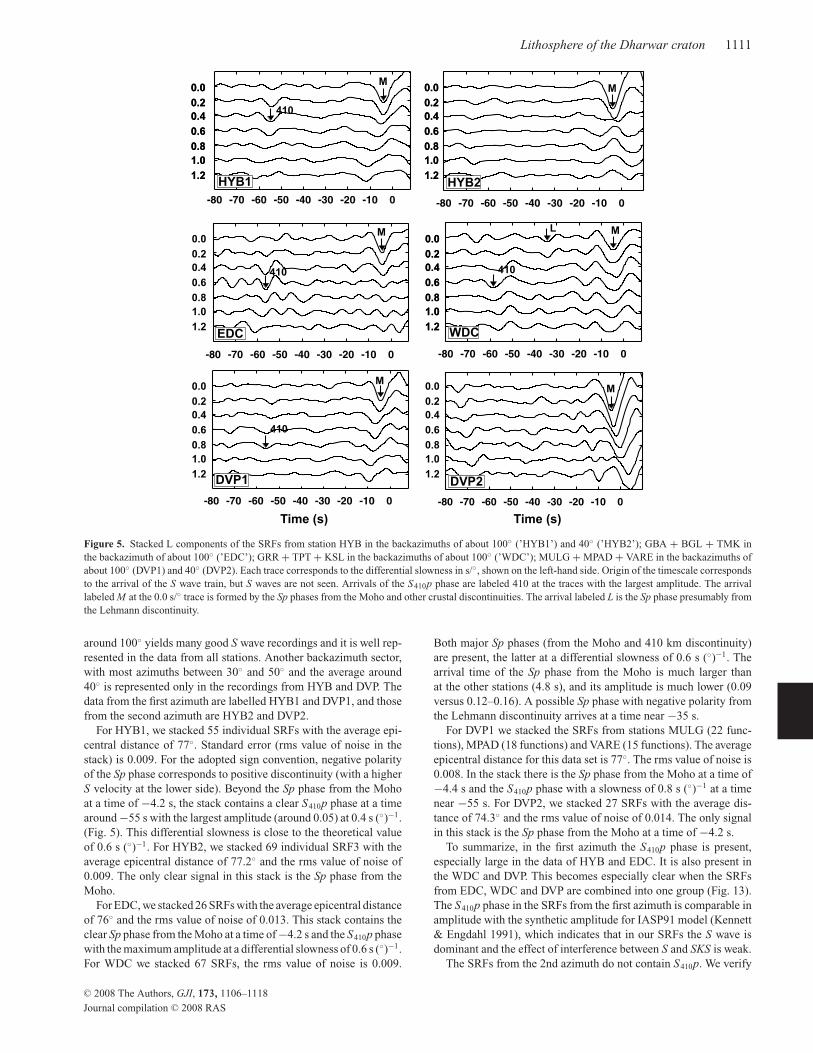
Figure 5. Stacked L components of the SRFs from station HYB in the backazimuths of about 100◦ (’HYB1’) and 40◦ (’HYB2’); GBA + BGL + TMK in

the backazimuth of about 100◦ (’EDC’); GRR + TPT + KSL in the backazimuths of about 100◦ (’WDC’); MULG + MPAD + VARE in the backazimuths of

about 100◦ (DVP1) and 40◦ (DVP2). Each trace corresponds to the differential slowness in s/◦, shown on the left-hand side. Origin of the timescale corresponds

to the arrival of the S wave train, but S waves are not seen. Arrivals of the S410p phase are labeled 410 at the traces with the largest amplitude. The arrival

labeled M at the 0.0 s/◦ trace is formed by the Sp phases from the Moho and other crustal discontinuities. The arrival labeled L is the Sp phase presumably from

the Lehmann discontinuity.

around 100◦ yields many good S wave recordings and it is well rep-

resented in the data from all stations. Another backazimuth sector,

with most azimuths between 30◦ and 50◦ and the average around

40◦ is represented only in the recordings from HYB and DVP. The

data from the first azimuth are labelled HYB1 and DVP1, and those

from the second azimuth are HYB2 and DVP2.

For HYB1, we stacked 55 individual SRFs with the average epi-

central distance of 77◦. Standard error (rms value of noise in the

stack) is 0.009. For the adopted sign convention, negative polarity

of the Sp phase corresponds to positive discontinuity (with a higher

S velocity at the lower side). Beyond the Sp phase from the Moho

at a time of −4.2 s, the stack contains a clear S410p phase at a time

around −55 s with the largest amplitude (around 0.05) at 0.4 s (◦)−1.

(Fig. 5). This differential slowness is close to the theoretical value

of 0.6 s (◦)−1. For HYB2, we stacked 69 individual SRF3 with the

average epicentral distance of 77.2◦ and the rms value of noise of

0.009. The only clear signal in this stack is the Sp phase from the

Moho.

For EDC, we stacked 26 SRFs with the average epicentral distance

of 76◦ and the rms value of noise of 0.013. This stack contains the

clear Sp phase from the Moho at a time of −4.2 s and the S410p phase

with the maximum amplitude at a differential slowness of 0.6 s (◦)−1.

For WDC we stacked 67 SRFs, the rms value of noise is 0.009.

Both major Sp phases (from the Moho and 410 km discontinuity)

are present, the latter at a differential slowness of 0.6 s (◦)−1. The

arrival time of the Sp phase from the Moho is much larger than

at the other stations (4.8 s), and its amplitude is much lower (0.09

versus 0.12–0.16). A possible Sp phase with negative polarity from

the Lehmann discontinuity arrives at a time near −35 s.

For DVP1 we stacked the SRFs from stations MULG (22 func-

tions), MPAD (18 functions) and VARE (15 functions). The average

epicentral distance for this data set is 77◦. The rms value of noise is

0.008. In the stack there is the Sp phase from the Moho at a time of

−4.4 s and the S410p phase with a slowness of 0.8 s (◦)−1 at a time

near −55 s. For DVP2, we stacked 27 SRFs with the average dis-

tance of 74.3◦ and the rms value of noise of 0.014. The only signal

in this stack is the Sp phase from the Moho at a time of −4.2 s.

To summarize, in the first azimuth the S410p phase is present,

especially large in the data of HYB and EDC. It is also present in

the WDC and DVP. This becomes especially clear when the SRFs

from EDC, WDC and DVP are combined into one group (Fig. 13).

The S410p phase in the SRFs from the first azimuth is comparable in

amplitude with the synthetic amplitude for IASP91 model (Kennett

& Engdahl 1991), which indicates that in our SRFs the S wave is

dominant and the effect of interference between S and SKS is weak.

The SRFs from the 2nd azimuth do not contain S410p. We verify

C© 2008 The Authors, GJI, 173, 1106–1118



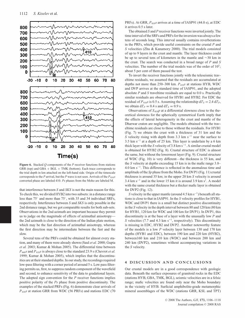
Figure 6. Stacked Q components of the P receiver functions from stations

GRR (top) and GBA + BGL + TMK (bottom). Each trace corresponds to

the trial depth in km attached on the left-hand side. Origin of the timescale

corresponds to the P arrival, but the P wave is not seen. Arrivals of the P410sconverted phase are labeled 410. Ps phases from the Moho are labeled M.

that interference between S and SKS is not the main reason for this.

To check this, we divided HYB2 into two subsets: in a distance range

less than 75◦ and more than 75◦, with 35 and 34 individual SRFs,

respectively. Interference between S and SKS is only possible in the

2nd distance range, but we got comparable results for both sub-sets.

Observations in the 2nd azimuth are important because they permit

us to judge on the magnitude of effects of azimuthal anisotropy—

the 2nd azimuth is close to the direction of the Indian plate motion,

which may be the fast direction of azimuthal anisotropy, whereas

the first direction may be intermediate between the fast and the

slow.

Several tens of the PRFs could be obtained for almost every sta-

tion, and many of them were already shown (Saul et al. 2000; Gupta

et al. 2003; Kumar & Mohan 2005). The differential time between

P660s and P410s is always close to the standard 23.9 s (Chevrot et al.1999; Kumar & Mohan 2005), which implies that the discontinu-

ities are at their standard depths. In our study, the recordings required

low-pass filtering with a corner period of around 5 s. Low pass filter-

ing permits us, first, to suppress random component of the wavefield

and second, to enhance sensitivity of the data to gradational layers.

The adopted sign convention for the P receiver functions implies

positive polarity of the Ps phase from positive discontinuity. The

examples of the stacked PRFs (Fig. 6) demonstrate clear arrivals of

P410s at station GRR from WDC (56 PRFs) and stations EDC (70

PRFs). At GRR, P410s arrives at a time of IASP91 (44.0 s), at EDC

it arrives 0.5 s later.

The obtained S and P receiver functions were inverted jointly. The

time interval of the SRFs and PRFs for the inversion was always a few

tens of seconds long. This interval usually contains reverberations

in the PRFs, which provide useful constraints on the crustal P and

S velocities (Zhu & Kanamory 2000). The trial models consisted

of up to 9 layers in the crust and mantle. The layer thickness could

be up to several tens of kilometers in the mantle and ∼30 km in

the crust. The search was conducted in a broad range of P and Svelocities. The number of the trial models was of the order of 105;

about 5 per cent of them passed the test.

To invert the receiver functions jointly with the teleseismic trav-

eltime residuals, we assumed that the residuals are accumulated at

depths not more than 250–300 km. P410s at stations HYB, WDC

and DVP arrives at the standard time of IASP91, and the adopted

absolute P and S traveltime residuals are equal to 0.0 s. Practically

similar residuals are observed for HYB1 and HYB2. For EDC the

residual of P410s is 0.5 s. Assuming the relationship dTS = 2.4 dTP,

we obtain dTP = 0.4 s and dTS = 0.9 s.

Observations of S410p at a differential slowness close to the the-

oretical slowness for the spherically symmetrical Earth imply that

the effects of lateral heterogeneity in the crust and mantle of the

Dharwar craton are negligible. The models obtained with the trav-

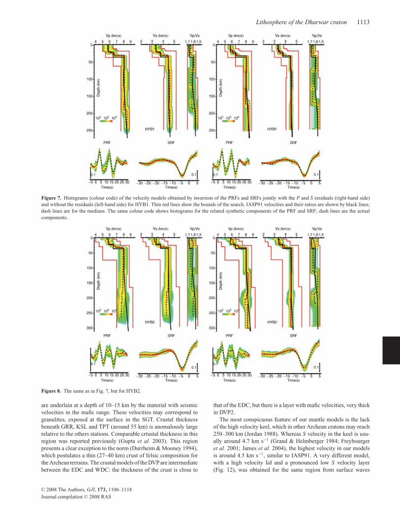
eltime residuals are close to those without the residuals. For HYB1

(Fig. 7) we obtain the crust with a thickness of 31 km and the

S velocity rising with depth from 3.3 km s−1 near the surface to

3.5 km s−1 at a depth of 25 km. This layer is underlain by a 6 km

thick layer with the S velocity of 3.8 km s−1. A similar crustal model

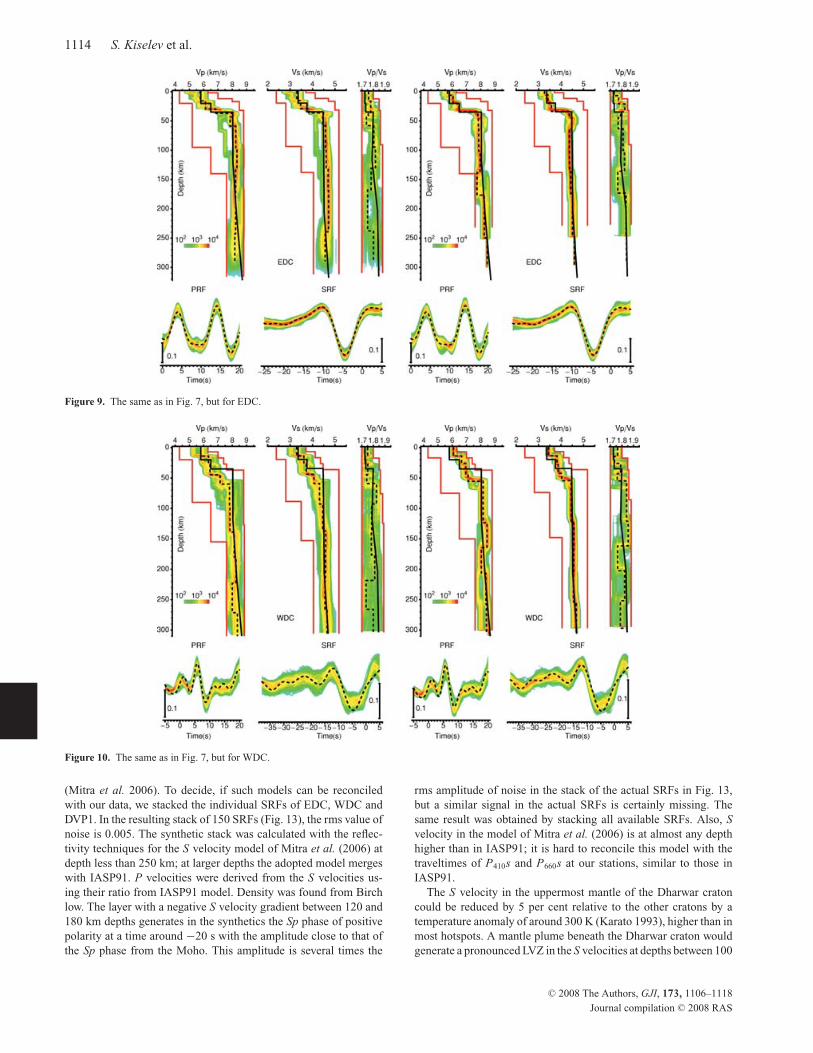
is obtained for HYB2 (Fig. 8). Crustal structure of EDC is almost

the same, but without the lowermost layer (Fig. 9). Crustal structure

of WDC (Fig. 10) is very different—the thickness is 55 km, and

the S velocity at depths exceeding 15 km is in the mafic range 3.8–

4.0 km s−1. This difference is reflected in the anomalous time and

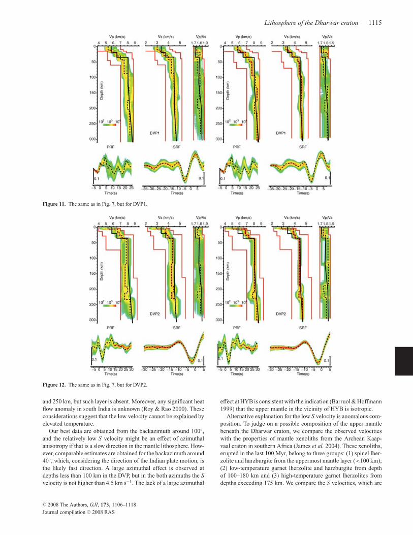
amplitude of the Sp phase from the Moho. For DVP1 (Fig. 11) crustal

thickness is around 35 km; in the upper 20 km S velocity is around

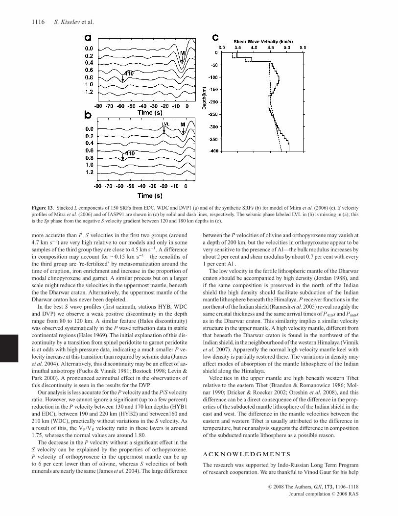
3.4 km s−1 and in the lower 15 km it is around 3.9 km s1. A model

with the same crustal thickness but a thicker mafic layer is obtained

for DVP2 (Fig. 12).

S velocity in the upper mantle (around 4.5 km s−1) beneath all sta-

tions is close to that in IASP91. In the S velocity profiles for HYB1,

WDC and DVP1 there is a small but distinct positive discontinuity

in the S velocity in the depth interval between 80 and 120 km (80 km

for HYB1, 120 km for WDC and 100 km for DVP1). In DVP1, this

discontinuity is at the base of a layer with the unusually low P and

S velocities (7.7 and 4.3 km s−1, respectively). This discontinuity

is missing in EDC, HYB2 and DVP2. Another noteworthy feature

of the models is a low P velocity layer between 130 and 170 km

depths (HYB1 and EDC), between 190 km and 220 km (HYB2),

between160 km and 210 km (WDC) and between 200 km and

240 km (DVP2), sometimes without accompanying variations in

the S velocity.

4 D I S C U S S I O N A N D C O N C L U S I O N S

Our crustal models are in a good correspondence with geologic

data. Beneath the surface exposures of granitoid rocks in the EDC

(stations HYB, GBA, TMK, BGL), seismic velocities are in a felsic

range; mafic velocities are found only near the Moho boundary

in the vicinity of HYB. Surficial amphibolite-grade metamorphic

mineral assemblages of the WDC (stations GRR, KSL and TPT)

C© 2008 The Authors, GJI, 173, 1106–1118



Figure 7. Histograms (colour code) of the velocity models obtained by inversion of the PRFs and SRFs jointly with the P and S residuals (right-hand side)

and without the residuals (left-hand side) for HYB1. Thin red lines show the bounds of the search. IASP91 velocities and their ratios are shown by black lines;

dash lines are for the medians. The same colour code shows histograms for the related synthetic components of the PRF and SRF; dash lines are the actual

components.

Figure 8. The same as in Fig. 7, but for HYB2.

are underlain at a depth of 10–15 km by the material with seismic

velocities in the mafic range. These velocities may correspond to

granulites, exposed at the surface in the SGT. Crustal thickness

beneath GRR, KSL and TPT (around 55 km) is anomalously large

relative to the others stations. Comparable crtustal thickness in this

region was reported previously (Gupta et al. 2003). This region

presents a clear exception to the norm (Durrheim & Mooney 1994),

which postulates a thin (27–40 km) crust of felsic composition for

the Archean terrains. The crustal models of the DVP are intermediate

between the EDC and WDC: the thickness of the crust is close to

that of the EDC, but there is a layer with mafic velocities, very thick

in DVP2.

The most conspicuous feature of our mantle models is the lack

of the high velocity keel, which in other Archean cratons may reach

250–300 km (Jordan 1988). Whereas S velocity in the keel is usu-

ally around 4.7 km s−1 (Grand & Helmberger 1984; Freybourger

et al. 2001; James et al. 2004), the highest velocity in our models

is around 4.5 km s−1, similar to IASP91. A very different model,

with a high velocity lid and a pronounced low S velocity layer

(Fig. 12), was obtained for the same region from surface waves

C© 2008 The Authors, GJI, 173, 1106–1118



Figure 9. The same as in Fig. 7, but for EDC.

Figure 10. The same as in Fig. 7, but for WDC.

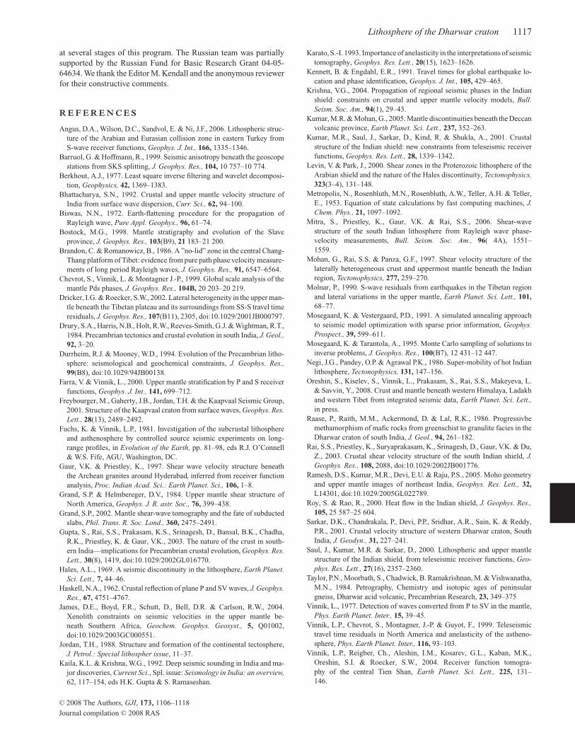
(Mitra et al. 2006). To decide, if such models can be reconciled

with our data, we stacked the individual SRFs of EDC, WDC and

DVP1. In the resulting stack of 150 SRFs (Fig. 13), the rms value of

noise is 0.005. The synthetic stack was calculated with the reflec-

tivity techniques for the S velocity model of Mitra et al. (2006) at

depth less than 250 km; at larger depths the adopted model merges

with IASP91. P velocities were derived from the S velocities us-

ing their ratio from IASP91 model. Density was found from Birch

low. The layer with a negative S velocity gradient between 120 and

180 km depths generates in the synthetics the Sp phase of positive

polarity at a time around −20 s with the amplitude close to that of

the Sp phase from the Moho. This amplitude is several times the

rms amplitude of noise in the stack of the actual SRFs in Fig. 13,

but a similar signal in the actual SRFs is certainly missing. The

same result was obtained by stacking all available SRFs. Also, Svelocity in the model of Mitra et al. (2006) is at almost any depth

higher than in IASP91; it is hard to reconcile this model with the

traveltimes of P410s and P660s at our stations, similar to those in

IASP91.

The S velocity in the uppermost mantle of the Dharwar craton

could be reduced by 5 per cent relative to the other cratons by a

temperature anomaly of around 300 K (Karato 1993), higher than in

most hotspots. A mantle plume beneath the Dharwar craton would

generate a pronounced LVZ in the S velocities at depths between 100

C© 2008 The Authors, GJI, 173, 1106–1118



Figure 11. The same as in Fig. 7, but for DVP1.

Figure 12. The same as in Fig. 7, but for DVP2.

and 250 km, but such layer is absent. Moreover, any significant heat

flow anomaly in south India is unknown (Roy & Rao 2000). These

considerations suggest that the low velocity cannot be explained by

elevated temperature.

Our best data are obtained from the backazimuth around 100◦,

and the relatively low S velocity might be an effect of azimuthal

anisotropy if that is a slow direction in the mantle lithosphere. How-

ever, comparable estimates are obtained for the backazimuth around

40◦, which, considering the direction of the Indian plate motion, is

the likely fast direction. A large azimuthal effect is observed at

depths less than 100 km in the DVP, but in the both azimuths the Svelocity is not higher than 4.5 km s−1. The lack of a large azimuthal

effect at HYB is consistent with the indication (Barruol & Hoffmann

1999) that the upper mantle in the vicinity of HYB is isotropic.

Alternative explanation for the low S velocity is anomalous com-

position. To judge on a possible composition of the upper mantle

beneath the Dharwar craton, we compare the observed velocities

with the properties of mantle xenoliths from the Archean Kaap-

vaal craton in southern Africa (James et al. 2004). These xenoliths,

erupted in the last 100 Myr, belong to three groups: (1) spinel lher-

zolite and harzburgite from the uppermost mantle layer (<100 km);

(2) low-temperature garnet lherzolite and harzburgite from depth

of 100–180 km and (3) high-temperature garnet lherzolites from

depths exceeding 175 km. We compare the S velocities, which are

C© 2008 The Authors, GJI, 173, 1106–1118



Figure 13. Stacked L components of 150 SRFs from EDC, WDC and DVP1 (a) and of the synthetic SRFs (b) for model of Mitra et al. (2006) (c). S velocity

profiles of Mitra et al. (2006) and of IASP91 are shown in (c) by solid and dash lines, respectively. The seismic phase labeled LVL in (b) is missing in (a); this

is the Sp phase from the negative S velocity gradient between 120 and 180 km depths in (c).

more accurate than P. S velocities in the first two groups (around

4.7 km s−1) are very high relative to our models and only in some

samples of the third group they are close to 4.5 km s−1. A difference

in composition may account for ∼0.15 km s−1—the xenoliths of

the third group are ’re-fertilized’ by metasomatization around the

time of eruption, iron enrichment and increase in the proportion of

modal clinopyroxene and garnet. A similar process but on a larger

scale might reduce the velocities in the uppermost mantle, beneath

the the Dharwar craton. Alternatively, the uppermost mantle of the

Dharwar craton has never been depleted.

In the best S wave profiles (first azimuth, stations HYB, WDC

and DVP) we observe a weak positive discontinuity in the depth

range from 80 to 120 km. A similar feature (Hales discontinuity)

was observed systematically in the P wave refraction data in stable

continental regions (Hales 1969). The initial explanation of this dis-

continuity by a transition from spinel peridotite to garnet peridotite

is at odds with high pressure data, indicating a much smaller P ve-

locity increase at this transition than required by seismic data (James

et al. 2004). Alternatively, this discontinuity may be an effect of az-

imuthal anisotropy (Fuchs & Vinnik 1981; Bostock 1998; Levin &

Park 2000). A pronounced azimuthal effect in the observations of

this discontinuity is seen in the results for the DVP.

Our analysis is less accurate for the P velocity and the P/S velocity

ratio. However, we cannot ignore a significant (up to a few percent)

reduction in the P velocity between 130 and 170 km depths (HYB1

and EDC), between 190 and 220 km (HYB2) and between160 and

210 km (WDC), practically without variations in the S velocity. As

a result of this, the VP/VS velocity ratio in these layers is around

1.75, whereas the normal values are around 1.80.

The decrease in the P velocity without a significant effect in the

S velocity can be explained by the properties of orthopyroxene.

P velocity of orthopyroxene in the uppermost mantle can be up

to 6 per cent lower than of olivine, whereas S velocities of both

minerals are nearly the same (James et al. 2004). The large difference

between the P velocities of olivine and orthopyroxene may vanish at

a depth of 200 km, but the velocities in orthopyroxene appear to be

very sensitive to the presence of Al—the bulk modulus increases by

about 2 per cent and shear modulus by about 0.7 per cent with every

1 per cent Al .

The low velocity in the fertile lithospheric mantle of the Dharwar

craton should be accompanied by high density (Jordan 1988), and

if the same composition is preserved in the north of the Indian

shield the high density should facilitate subduction of the Indian

mantle lithosphere beneath the Himalaya. P receiver functions in the

northeast of the Indian shield (Ramesh et al. 2005) reveal roughly the

same crustal thickness and the same arrival times of P410s and P660sas in the Dharwar craton. This similarity implies a similar velocity

structure in the upper mantle. A high velocity mantle, different from

that beneath the Dharwar craton is found in the northwest of the

Indian shield, in the neighbourhood of the western Himalaya (Vinnik

et al. 2007). Apparently the normal high velocity mantle keel with

low density is partially restored there. The variations in density may

affect modes of absorption of the mantle lithosphere of the Indian

shield along the Himalaya.

Velocities in the upper mantle are high beneath western Tibet

relative to the eastern Tibet (Brandon & Romanowicz 1986; Mol-

nar 1990; Dricker & Roecker 2002; Oreshin et al. 2008), and this

difference can be a direct consequence of the difference in the prop-

erties of the subducted mantle lithosphere of the Indian shield in the

east and west. The difference in the mantle velocities between the

eastern and western Tibet is usually attributed to the difference in

temperature, but our analysis suggests the difference in composition

of the subducted mantle lithosphere as a possible reason.

A C K N O W L E D G M E N T S

The research was supported by Indo-Russian Long Term Program

of research cooperation. We are thankful to Vinod Gaur for his help

C© 2008 The Authors, GJI, 173, 1106–1118



at several stages of this program. The Russian team was partially

supported by the Russian Fund for Basic Research Grant 04-05-

64634. We thank the Editor M. Kendall and the anonymous reviewer

for their constructive comments.

R E F E R E N C E S

Angus, D.A., Wilson, D.C., Sandvol, E. & Ni, J.F., 2006. Lithospheric struc-

ture of the Arabian and Eurasian collision zone in eastern Turkey from

S-wave receiver functions, Geophys. J. Int., 166, 1335–1346.

Barruol, G. & Hoffmann, R., 1999. Seismic anisotropy beneath the geoscope

stations from SKS splitting, J. Geophys. Res., 104, 10 757–10 774.

Berkhout, A.J., 1977. Least square inverse filtering and wavelet decomposi-

tion, Geophysics, 42, 1369–1383.

Bhattacharya, S.N., 1992. Crustal and upper mantle velocity structure of

India from surface wave dispersion, Curr. Sci., 62, 94–100.

Biswas, N.N., 1972. Earth-flattening procedure for the propagation of

Rayleigh wave, Pure Appl. Geophys., 96, 61–74.

Bostock, M.G., 1998. Mantle stratigraphy and evolution of the Slave

province, J. Geophys. Res., 103(B9), 21 183–21 200.

Brandon, C. & Romanowicz, B., 1986. A ”no-lid” zone in the central Chang-

Thang platform of Tibet: evidence from pure path phase velocity measure-

ments of long period Rayleigh waves, J. Geophys. Res., 91, 6547–6564.

Chevrot, S., Vinnik, L. & Montagner J.-P., 1999. Global scale analysis of the

mantle Pds phases, J. Geophys. Res., 104B, 20 203–20 219.

Dricker, I.G. & Roecker, S.W., 2002. Lateral heterogeneity in the upper man-

tle beneath the Tibetan plateau and its surroundings from SS-S travel time

residuals, J. Geophys. Res., 107(B11), 2305, doi:10.1029/2001JB000797.

Drury, S.A., Harris, N.B., Holt, R.W., Reeves-Smith, G.J. & Wightman, R.T.,

1984. Precambrian tectonics and crustal evolution in south India, J. Geol.,92, 3–20.

Durrheim, R.J. & Mooney, W.D., 1994. Evolution of the Precambrian litho-

sphere: seismological and geochemical constraints, J. Geophys. Res.,99(B8), doi:10.1029/94JB00138.

Farra, V. & Vinnik, L., 2000. Upper mantle stratification by P and S receiver

functions, Geophys. J. Int., 141, 699–712.

Freybourger, M., Gaherty, J.B., Jordan, T.H. & the Kaapvaal Seismic Group,

2001. Structure of the Kaapvaal craton from surface waves, Geophys. Res.Lett., 28(13), 2489–2492.

Fuchs, K. & Vinnik, L.P., 1981. Investigation of the subcrustal lithosphere

and asthenosphere by controlled source seismic experiments on long-

range profiles, in Evolution of the Earth, pp. 81–98, eds R.J. O’Connell

& W.S. Fife, AGU, Washington, DC.

Gaur, V.K. & Priestley, K., 1997. Shear wave velocity structure beneath

the Archean granites around Hyderabad, inferred from receiver function

analysis, Proc. Indian Acad. Sci.: Earth Planet. Sci., 106, 1–8.

Grand, S.P. & Helmbereger, D.V., 1984. Upper mantle shear structure of

North America, Geophys. J. R. astr. Soc., 76, 399–438.

Grand, S.P., 2002. Mantle shear-wave tomography and the fate of subducted

slabs, Phil. Trans. R. Soc. Lond., 360, 2475–2491.

Gupta, S., Rai, S.S., Prakasam, K.S., Srinagesh, D., Bansal, B.K., Chadha,

R.K., Priestley, K. & Gaur, V.K., 2003. The nature of the crust in south-

ern India—implications for Precambrian crustal evolution, Geophys. Res.Lett., 30(8), 1419, doi:10.1029/2002GL016770.

Hales, A.L., 1969. A seismic discontinuity in the lithosphere, Earth Planet.Sci. Lett., 7, 44–46.

Haskell, N.A., 1962. Crustal reflection of plane P and SV waves, J. Geophys.Res., 67, 4751–4767.

James, D.E., Boyd, F.R., Schutt, D., Bell, D.R. & Carlson, R.W., 2004.

Xenolith constraints on seismic velocities in the upper mantle be-

neath Southern Africa, Geochem. Geophys. Geosyst., 5, Q01002,

doi:10.1029/2003GC000551.

Jordan, T.H., 1988. Structure and formation of the continental tectosphere,

J. Petrol.: Special lithospher issue, 11–37.

Kaila, K.L. & Krishna, W.G., 1992. Deep seismic sounding in India and ma-

jor discoveries, Current Sci., Spl. issue: Seismology in India: an overview,62, 117–154, eds H.K. Gupta & S. Ramaseshan.

Karato, S.-I. 1993. Importance of anelasticity in the interpretations of seismic

tomography, Geophys. Res. Lett., 20(15), 1623–1626.

Kennett, B. & Engdahl, E.R., 1991. Travel times for global earthquake lo-

cation and phase identification, Geophys. J. Int., 105, 429–465.

Krishna, V.G., 2004. Propagation of regional seismic phases in the Indian

shield: constraints on crustal and upper mantle velocity models, Bull.Seism. Soc. Am., 94(1), 29–43.

Kumar, M.R. & Mohan, G., 2005. Mantle discontinuities beneath the Deccan

volcanic province, Earth Planet. Sci. Lett., 237, 352–263.

Kumar, M.R., Saul, J., Sarkar, D., Kind, R. & Shukla, A., 2001. Crustal

structure of the Indian shield: new constraints from teleseismic receiver

functions, Geophys. Res. Lett., 28, 1339–1342.

Levin, V. & Park, J., 2000. Shear zones in the Proterozoic lithosphere of the

Arabian shield and the nature of the Hales discontinuity, Tectonophysics,323(3–4), 131–148.

Metropolis, N., Rosenbluth, M.N., Rosenbluth, A.W., Teller, A.H. & Teller,

E., 1953. Equation of state calculations by fast computing machines, J.Chem. Phys., 21, 1097–1092.

Mitra, S., Priestley, K., Gaur, V.K. & Rai, S.S., 2006. Shear-wave

structure of the south Indian lithosphere from Rayleigh wave phase-

velocity measurements, Bull. Seism. Soc. Am., 96( 4A), 1551–

1559.

Mohan, G., Rai, S.S. & Panza, G.F., 1997. Shear velocity structure of the

laterally heterogeneous crust and uppermost mantle beneath the Indian

region, Tectonophysics, 277, 259–270.

Molnar, P., 1990. S-wave residuals from earthquakes in the Tibetan region

and lateral variations in the upper mantle, Earth Planet. Sci. Lett., 101,68–77.

Mosegaard, K. & Vestergaard, P.D., 1991. A simulated annealing approach

to seismic model optimization with sparse prior information, Geophys.Prospect., 39, 599–611.

Mosegaard, K. & Tarantola, A., 1995. Monte Carlo sampling of solutions to

inverse problems, J. Geophys. Res., 100(B7), 12 431–12 447.

Negi, J.G., Pandey, O.P. & Agrawal P.K., 1986. Super-mobility of hot Indian

lithosphere, Tectonophysics, 131, 147–156.

Oreshin, S., Kiselev, S., Vinnik, L., Prakasam, S., Rai, S.S., Makeyeva, L.

& Savvin, Y., 2008. Crust and mantle beneath western Himalaya, Ladakh

and western Tibet from integrated seismic data, Earth Planet. Sci. Lett.,in press.

Raase, P., Raith, M.M., Ackermond, D. & Lal, R.K., 1986. Progressivbe

methamorphism of mafic rocks from greenschist to granulite facies in the

Dharwar craton of south India, J. Geol., 94, 261–182.

Rai, S.S., Priestley, K., Suryaprakasam, K., Srinagesh, D., Gaur, V.K. & Du,

Z., 2003. Crustal shear velocity structure of the south Indian shield, J.Geophys. Res., 108, 2088, doi:10.1029/2002JB001776.

Ramesh, D.S., Kumar, M.R., Devi, E.U. & Raju, P.S., 2005. Moho geometry

and upper mantle images of northeast India, Geophys. Res. Lett., 32,L14301, doi:10.1029/2005GL022789.

Roy, S. & Rao, R., 2000. Heat flow in the Indian shield, J. Geophys. Res.,105, 25 587–25 604.

Sarkar, D.K., Chandrakala, P., Devi, P.P., Sridhar, A.R., Sain, K. & Reddy,

P.R., 2001. Crustal velocity structure of western Dharwar craton, South

India, J. Geodyn., 31, 227–241.

Saul, J., Kumar, M.R. & Sarkar, D., 2000. Lithospheric and upper mantle

structure of the Indian shield, from teleseismic receiver functions, Geo-phys. Res. Lett., 27(16), 2357–2360.

Taylor, P.N., Moorbath, S., Chadwick, B. Ramakrishnan, M. & Vishwanatha,

M.N., 1984. Petrography, Chemistry and isotopic ages of peninsular

gneiss, Dharwar acid volcanic, Precambrian Research, 23, 349–375

Vinnik, L., 1977. Detection of waves converted from P to SV in the mantle,

Phys. Earth Planet. Inter., 15, 39–45.

Vinnik, L.P., Chevrot, S., Montagner, J.-P. & Guyot, F., 1999. Teleseismic

travel time residuals in North America and anelasticity of the astheno-

sphere, Phys. Earth Planet. Inter., 116, 93–103.

Vinnik, L.P., Reigber, Ch., Aleshin, I.M., Kosarev, G.L., Kaban, M.K.,

Oreshin, S.I. & Roecker, S.W., 2004. Receiver function tomogra-

phy of the central Tien Shan, Earth Planet. Sci. Lett., 225, 131–

146.

C© 2008 The Authors, GJI, 173, 1106–1118



Vinnik, L.P., Aleshin, I.M., Kaban, M.K., Kiselev, S.G., Kosarev, G.L.,

Oreshin, S.I. & Reigber, Ch., 2006. Crust and mantle of the Tien Shan

from the data of the receiver function tomography, Izvestia, Phys. SolidEarth, 42, 639–651.

Vinnik, L., Singh, A., Kiselev, S. & Kumar, M.R., 2007. Upper mantle

beneath foothills of the western Himalaya: subducted lithospheric slab or

a keel of the Indian shield? Geophys. J. Int., 171, 1162–1171.

Wilson, D.C., Angus, D.A., Ni, J. & Grand, S., 2006. Constraints on the

interpretation of S-to-P receiver finctions, Geophys. J. Int., 165, 969–

980.

Zhu, L. & Kanamori, H., 2000. Moho depth variation in southern California

from teleseismic receiver functions, J. Geophys. Res., 105, 2969–2980.

Zhou, L., Chen, W.-P. & Ozalaybey, S., 2000. Seismic properties of the

Central Indian shield, Bull. Seism. Soc. Am., 90, 1295–1304.

C© 2008 The Authors, GJI, 173, 1106–1118


Lithosphere of the Dharwar craton by joint inversion of P and S receiver functions

Documents

Transcript of Lithosphere of the Dharwar craton by joint inversion of P and S receiver functions