Seismic Tomography of the Lithosphere with Body Waves

Seismic Tomography of the Lithosphere with Body Waves

CLIFFORD H. THURBER1

Abstract—A pair of papers in 1976 lead-authored by Kei Aki heralded the beginning of the field of

seismic tomography of the lithosphere. The 1976 paper by Aki, Christoffersson, and Husebye introduced a

simple and approximate yet elegant technique for using body-wave arrival times from teleseismic

earthquakes to infer the three-dimensional (3-D) seismic velocity heterogeneities beneath a seismic array or

network (teleseismic tomography). Similarly, a 1976 paper by Aki and Lee presented a method for

inferring 3-D structure beneath a seismic network using body-wave arrival times from local earthquakes

(local earthquake tomography). Following these landmark papers, many dozens of papers and numerous

books have been published presenting exciting applications of and/or innovative improvements to the

methods of teleseismic and local earthquake tomography, many by Aki’s students.

This paper presents a brief review of these two types of tomography methods, discussing some of the

underlying assumptions and limitations. Thereafter some of the significant methodological developments

are traced over the past two and a half decades, and some of the applications of tomography that have

reaped the benefits of these developments are highlighted. One focus is on the steady improvement in

structural resolution and inference power brought about by the increased number and quality of seismic

stations, and in particular the value of utilizing shear waves. The paper concludes by discussing exciting

new scientific projects in which seismic tomography will play a major role — the San Andreas Fault

Observatory at Depth (SAFOD) and USArray, the initial components of Earthscope.

Key words: Tomography, body waves, teleseismic, local earthquake.

Introduction

In 1974, Kei Aki visited NORSAR, and the availability of high-quality seismic

data from a dense array combined with Aki’s knowledge of inverse theory led to the

‘‘birth’’ of modern seismic tomography. Working together with A. Christoffersson

and E. Husebye, the three developed what has become known as the ACH teleseismic

tomography method. The method uses the arrival times of P waves at a seismic array

or network to infer three-dimensional (3-D) velocity heterogeneities in the volume

beneath the stations. The team published their analyses of data from 2 arrays and

one regional network in 3 papers that appeared in 1976 and 1977 (AKI et al., 1976,

1977; HUSEBYE et al., 1976). As the story goes, the third paper in the series, which is

the one most widely cited, was intended to be published first, but a sign error in the

1Department of Geology and Geophysics, University of Wisconsin-Madison, 1215 W. Dayton St.,

Madison WI 53706, U.S.A. E-mail: [email protected]

Pure appl. geophys. 160 (2003) 717–737

0033 – 4553/03/040717 – 21

� Birkhauser Verlag, Basel, 2003

Pure and Applied Geophysics

data delayed its publication (EVANS and ACHAUER, 1993). Then in 1975, Aki spent

time at the U.S. Geological Survey in Menlo Park, California. Working together with

Willie Lee, the pair extended the ACH tomography method to the case of local

earthquakes. The local earthquake method utilizes P-wave arrival times from

earthquakes beneath a seismic network to infer the 3-D velocity structure in the

volume containing the earthquakes and stations. Their local earthquake tomography

paper was published in 1976 (AKI and LEE, 1976). I will refer to their approach as the

A&L method.

The author was fortunate to arrive at MIT in the fall of 1976. A number of

graduate students, both of Aki’s and of other faculty members, was either already or

soon to be working on applications of seismic tomography (although we did not call

it tomography at the time). Among this group were Bill Ellsworth, George Zandt,

Steve Roecker, Steve Taylor and myself. Computers at MIT were slowly making the

transition from punched cards to on-line disk storage and remote terminals, and

color graphics were done with Exacto knives and colored acetate sheets. How times

have changed!

The retirement of Kei Aki brings an opportunity to reflect on the brief history of

seismic tomography using body waves, with a focus on work involving his students

and their collaborators. The initial tomography methods made simplifying assump-

tions that have become generally unnecessary due to advances in methodology and

computer power. Local- and regional-scale applications were initially limited to

places where seismic arrays or networks were in place. However, the creation of the

Incorporated Research Institutions for Seismology (IRIS) portable seismic instru-

ment program, the Program for Array Seismic Studies of the Continental

Lithosphere (PASSCAL) (SMITH, 1986; FOWLER and PAVLIS, 1994), opened up

virtually unlimited opportunities for carrying out tomography studies in regions of

scientific interest. Now there may be the beginning of a new era of opportunity for

seismic tomography studies in the U.S. with the impending establishment of the

Earthscope program (HENYEY et al., 2000). With tomography components ranging

from the fine-scale structure of the San Andreas fault in the SAFOD project to the

broad-scale structure of the North American lithosphere in the USArray project,

Earthscope promises to provide the field of seismic tomography with unprecedented

data for imaging the internal structure of the earth.

Basic Tomography Methodology

Both teleseismic and local earthquake tomography make use of the arrival times

of body waves (P and/or S) to infer the seismic velocity structure. In the case of

teleseismic tomography, the earthquakes must be at relatively great distances from a

localized cluster of seismic stations, so that the waves incident on the array can be

treated as plane waves (Fig. 1a). With this assumption, it is only the structure

718 Clifford H. Thurber Pure appl. geophys.,

immediately beneath the stations that contributes to arrival time perturbations

(relative to a radially-symmetric model), and the source locations and origin times

need not be precisely known. I note that this assumption has been questioned by

MASSON and TRAMPERT (1997), who showed that travel times to the base of an ACH

model through a representative global 3-D velocity model could not adequately be

treated as a plane wave in some cases. However, this potential problem can be

avoided using the approach of WIDIYANTORO and VAN DER HILST (1997) or

BIJWAARD et al. (1998), by modeling coarse-scale global structure and fine-scale

regional structure simultaneously. In contrast, for local earthquake tomography, the

events and stations are in the same area (Fig. 1b). In this case, structure along the

entire path from event to station contributes to arrival time perturbations, and the

source location and origin time need to be treated formally as unknowns along with

the structure model.

For teleseismic tomography, the equations are written to separate the contribu-

tions to arrival time from inside versus outside the model:

t ¼ �ss þXNLs¼1

�ttsXMk¼1

Fsk 1þ Dukus

� �þ e ð1Þ

where t is the arrival time at the station, �ss is the arrival time at the base of the model(calculated from a standard earth model), �tts is the travel time through layer s in theunperturbed medium, Fsk is 1 if the ray in layer s has most of its length in block k andis otherwise zero, us is the slowness in layer s, Duk is the slowness perturbation inblock k, and e represents model errors and measurement errors. AKI et al. (1977)expressed this in matrix notation for a set of observations as

t ¼ �ss �G�mmþ m0iþ e ð2Þ

where t is the vector of arrival times,�ss is the vector of arrival times at the base of themodel, G is the relatively sparse matrix containing the appropriate �tts values, �mm is the

vector of fractional slowness deviations from the layer average in the blocks, m0 is the

travel time through the unperturbed model, i is a vector consisting of ones, and the

vector e contains the error terms. By rewriting equation (2) in terms of arrival timeresiduals and subtracting the average of the travel time residual over all stations for

each event from the left-hand side, Aki and Lee arrived at the relation

t� ¼ G� �mmþ e� ð3Þ

where * indicates the vector or matrix value minus the corresponding average. Thus

the ACH method inverts relative arrival time residuals for relative perturbations in

fractional slowness. This approach effectively removes error contributions from

inaccuracies in the standard earth model and in the source location and origin time.

For local earthquake tomography, the derivation of the equations is simpler

because no averaging is required to remove the source and outside-the-model path

Vol. 160, 2003 Lithosphere Tomography with Body Waves 719

a)

LOCAL NETWORK

� � � � �

❉❉

❉

❉❉

MODEL VOLUME

b)


terms, although the equations themselves are more complicated. The equations

relating residuals to model parameters can be written directly as

tobsij � tcalij ¼Xk

T ðkÞij

Dukuk

þ DT oj þ oTij

oxjD xj þ

oTijoyj

Dyj þoTijozj

Dzj ð4Þ

where the dependence of arrival time on source origin time and position is now an

explicit part of the system to be solved, entering in the form of the perturbation to

origin time (DT oj ) and the partial derivatives of travel time with respect to source

coordinates (e.g., oTij=oxj) times the corresponding coordinate perturbations (e.g.,DxjÞ. For a starting model that is a homogeneous and isotropic medium, as assumedin the A&L method, the derivatives are proportional to the corresponding direction

cosines of the vector connecting the source to the receiver. For the general case, the

derivatives are proportional to the direction cosines of the ray direction at the source

(THURBER, 1986).

The original ACH teleseismic and the A&L local earthquake methods both

involved single-step linearized inversions for the model parameters. This approach

allowed the use of linear inverse theory techniques for model estimation and model

resolution and uncertainty analysis. AKI et al. (1977) compared models obtained

using both a generalized inverse and a stochastic inverse. For the teleseismic case, the

system of equations is always linearly dependent due to the trade off between average

layer velocity and event origin times, consequently a simple least-squares solution

was impossible. The generalized inverse approach uses the non-zero singular values

of the G� matrix (equation (3)) to compute a least-squares solution, while the

stochastic inverse approach computes a damped least-squares solution using a

damping value equal to the ratio of the data variance to the solution variance (AKI

et al., 1977). AKI and LEE (1976) used just the stochastic inverse approach, because

their matrix was nonsingular but contained very small eigenvalues that would

amplify the effect of data errors on the model.

Advances in Seismic Tomography

There are a number of important aspects in which the methods and applications

of body-wave seismic tomography have been improved over the last 25 years. Some

of the advances I will discuss are improvements in the data, development of 3-D ray-

tracing techniques, the use of iterative (nonlinear) inversion, the extension to active-

Figure 1

(a) Geometry of the teleseismic tomography method. It is assumed that the P waves from teleseisms are

incident on the base of the model approximately as plane waves and are recorded on the surface by a dense

network. (b) Geometry of the local earthquake tomography method. The model volume contains both the

earthquakes and the stations.

b


source applications, and multiple-method integration. Other improvements include

the incorporation of interfaces (e.g., ZHAO et al., 1992) and the use of anisotropic

velocity models (e.g., HIRAHARA and ISHIKAWA, 1984).

Better data for tomography have arguably been the most important improve-

ment, because without better data the other advances would have been of relatively

limited use. Improvements in data have come in the form of additional instruments,

the use of 3-component sensors, and more accurate arrival time picks. These factors

allow for improved spatial resolution of structure, the ability to use S waves with

reliability, and a sharpening of imaged structure with reduced uncertainty,

respectively.

The development of the IRIS PASSCAL program in the U.S. and similar

instrument pool developments in other countries has had a tremendously positive

impact on the seismic tomography community. In the past, tomography studies were

restricted to regions with existing seismic networks (with data access often limited to

just those institutions operating the networks) or to a small number of institutions

fortunate to have field instruments. Now, any U.S. scientist has the opportunity to

propose and, if funded, carry out a seismic field project anywhere in the world

involving the collection of seismic data using PASSCAL instruments.

One of the key features of the PASSCAL and other modern instrument pools is

that 3-component instruments are the standard. As a result, S waves can be put to

use to image structure with nearly the same capability as P waves, the main

drawbacks being the presence of the P-coda noise interfering with precise S-wave

arrival time picks and the possibility of shear wave splitting adding uncertainties to

the data. The main value of S waves is the improved constraint on earthquake

locations provided by the addition of S arrivals (GOMBERG et al., 1990), which in

turn improves the imaging of structure, and the increased constraints on model

interpretation when 3-D models of both Vp and Vs (or Vp/Vs, equivalently Poisson’s

ratio) are available (EBERHART-PHILLIPS, 1990).

A study by ELLSWORTH (1977) demonstrated that a single-step inversion is

adequate for teleseismic tomography when the size of velocity perturbations is

relatively modest (less than 10%). The same is generally not true for local earthquake

tomography. Beginning with THURBER (1981) and ROECKER (1982), a number of

studies using synthetic models and data have shown that an iterative solution

incorporating 3-D ray tracing is required for local earthquake tomography. The

same is true for cross-borehole travel-time tomography, in which accounting for ray

bending is widely recognized as being important. In the local earthquake case, it is

even more important due to the coupling between structure and hypocenter locations

(KISSLING, 1988; THURBER, 1992).

In the early stages of development, limited computer power made the use of exact

ray-tracing techniques impractical. As a result, a variety of approximate ray-tracing

techniques were developed (THURBER and ELLSWORTH, 1980; UM and THURBER,

1987; PROTHERO et al., 1988). These methods achieved accuracies approaching that


of reading error (a few tenths of a second or less) for moderate path lengths (up to

60 km), so they remain widely used even today. Over time, efficient exact ray-tracing

(or more generally, travel time calculation) methods were developed. Examples

include 3-D finite difference (VIDALE, 1988, 1990; PODVIN and LECOMTE, 1991),

graph theory (MOSER, 1991), and perturbation methods (VIRIEUX et al., 1988;

SNIEDER and SAMBRIDGE, 1992). See THURBER and KISSLING (2000) for a review.

It is important to recognize that even the ‘‘exact’’ methods have limited accuracy.

HASLINGER and KISSLING (2001) and KISSLING et al. (2001) carried out extensive

tests of both exact and approximate ray-tracing techniques, involving reciprocity

tests on each method and comparing calculated travel times among methods. The

basic conclusion of their analyses is that all methods have comparable accuracy

variability for modest path lengths (�60 km), but the ‘‘exact’’ methods are superiorfor longer path lengths. They also noted that particular care must be taken regarding

differences in the way the velocity model is parameterized in order to be able to make

accurate comparisons among methods.

Seismic tomography was adapted to controlled-source problems in the 1980s.

Non-linear solutions are generally required, as in the local earthquake case.

Applications of controlled-source tomography include refraction, cross-borehole,

and vertical seismic profiling (VSP). A review of these methods and their applications

is beyond the scope of this paper.

Standard seismic tomography using first-arriving waves by itself provides only

limited insight into the nature of the subsurface. By its nature, it provides a smoothed

image of velocity structure, due to imperfect resolution, wavefront healing, etc. The

use of information from secondary arrivals (reflections, conversions) provides one

seismic approach for obtaining information about impedance structure, that is,

identifying discontinuities. One example will be presented in the following section.

Greater insight into the earth’s structure can also be gained via multidisciplinary

investigations. Two examples of methods that have proven useful in combination

with seismic tomography are magnetotellurics (MT) and laboratory and down-hole

measurements of seismic properties. EBERHART-PHILLIPS et al. (1990) compared

velocity and MT models for a 2-D section crossing the San Andreas fault through the

1989 Loma Prieta main shock region (Fig. 2). High-Vp rocks between the San

Andreas and Sargent faults were interpreted as mafic rocks due to their high

resistivity. Low- Vp rocks in a wedge southwest of the San Andreas were interpreted

as over-pressured marine sedimentary rocks due to their very high conductivity.

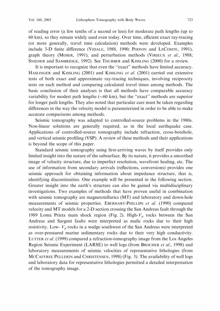
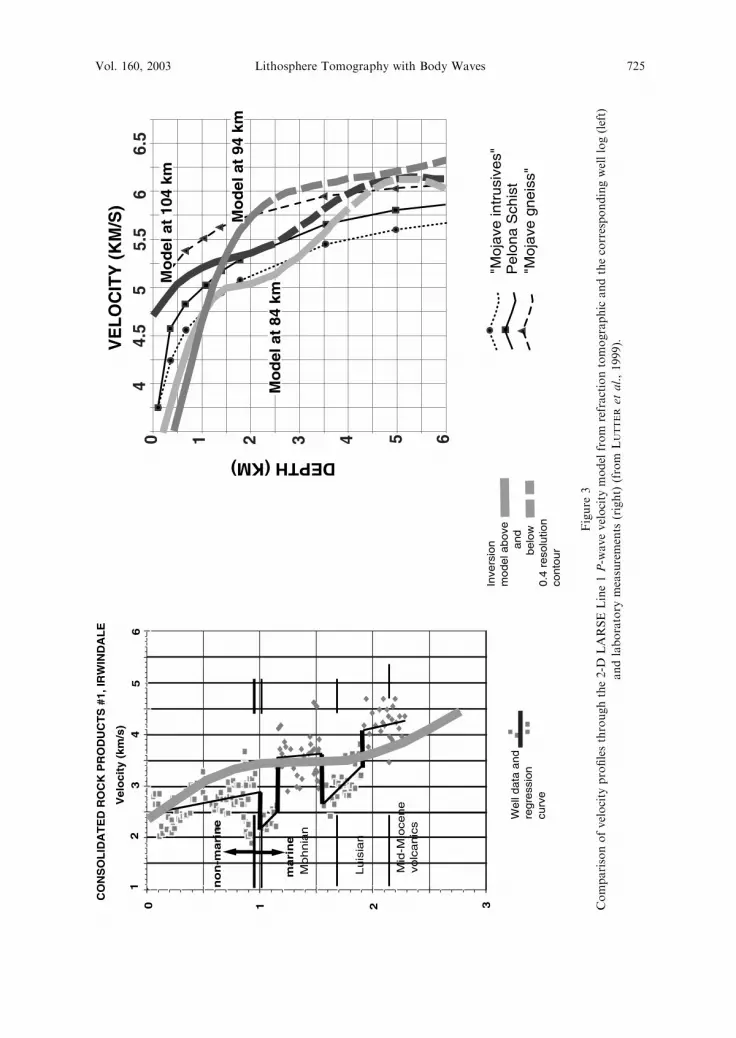
LUTTER et al. (1999) compared a refraction-tomography image from the Los Angeles

Region Seismic Experiment (LARSE) to well logs (from BROCHER et al., 1998) and

laboratory measurements of seismic velocities of representative lithologies (from

MCCAFFREE PELLERIN and CHRISTENSEN, 1998) (Fig. 3). The availability of well logs

and laboratory data for representative lithologies permitted a detailed interpretation

of the tomography image.


Applications of Seismic Tomography to Valles Caldera

Volcanic systems have been one of the key targets for seismic tomography studies

due to the desire to image the magma chambers at depth in the crust (IYER and

DAWSON, 1993). Aki’s student Peter Roberts carried out a field project in Valles

Caldera in collaboration with Mike Fehler of LANL (also an Aki student). They

used six instruments staged in two deployments along a linear profile across the

caldera (ROBERTS et al., 1991). Due to their limited teleseismic dataset, they used a

forward modeling approach, including a priori information on the shallow caldera

structure. Their final 2-D P-wave velocity model (Fig. 4) has a lens-shaped crustal

low-velocity zone (LVZ) with about a 35% velocity reduction compared to the

surrounding rock. The LVZ was interpreted to be the remnants of a cooling magma

chamber. The maximum width and minimum thickness of the LVZ are 17 km and 8

km, respectively.

Figure 2

Comparison of a 2-D magnetotelluric model with the corresponding slice through the P-wave velocity

tomography model contours for the Loma Prieta area (modified from EBERHART-PHILLIPS et al., 1990).

Note the excellent correspondence between the low-velocity basin and the low-resistivity units just SW of

the San Andreas fault (SAF) and the high-velocity ‘‘tongue’’ and the high resistivity unit between the SAF

and Sargent fault.


DEPTH (KM)

44.

55

5.5

66.

50 1 32 4 5 6

VE

LO

CIT

Y (

KM

/S)

"Mo

jave

gn

eis

s"P

elo

na

Sch

ist

"Mo

jave

intr

usi

ves"

Mo

del

at

94 k

m

Mo

del

at

84 k

m

Mo

del

at

104

km

Vel

oci

ty (

km/s

)

CO

NS

OL

IDA

TE

D R

OC

K P

RO

DU

CT

S #

1, IR

WIN

DA

LE

Mo

hn

ian

Lu

isia

n

Mid

-Mio

ce

ne

vo

lca

nic

s

12

34

50 1 2 3

no

n-m

ari

ne

ma

rin

e

Inve

rsio

nm

odel a

bove

and

belo

w0.4

reso

lutio

nco

nto

ur

Well

data

and

regre

ssio

ncu

rve

6

Figure3

Comparisonofvelocityprofilesthroughthe2-D

LARSELine1P-wavevelocitymodelfromrefractiontomographicandthecorrespondingwelllog(left)

andlaboratorymeasurements(right)(fromLUTTERetal.,1999).


The results of ROBERTS et al. (1991) helped lead to a much larger PASSCAL

teleseismic imaging project known as JTEX in the summers of 1993 and 1994. This

project involved Peter Roberts, Mike Fehler, and several coworkers an LANL, as

well as the author and his research group at UW. The 1993 JTEX pilot experiment,

with 22 stations on 2 crossing profiles (LUTTER et al., 1995), provided general

confirmation of the location, depth, size, and velocity contrast of the LVZ reported

by ROBERTS et al. (1991), using the ACH method to derive the velocity model.

With the complete JTEX teleseismic dataset, combining the 1993 and 1994 data

(Fig. 5a), STECK et al. (1998) modeled the 3-D structure of the caldera using a

nonlinear teleseismic tomography method. The principal features in the 3-D model

are a mid-crustal low velocity body, roughly (10 km)3 in size with a –35% velocity

contract, consistent with the 2-D results, and a second low velocity body near the

Moho (Fig. 5b). The authors combined the tomography model with geochemical

information to conclude that Valles Caldera recently received a new pulse of magma

from the upper mantle. Neither the 3-D geometry of the Valles magma chamber nor

Figure 4

2-D P-wave velocity model for the structure beneath Valles caldera (from ROBERTS et al., 1991). Note the

lens-shaped low-velocity zone in the mid-crust (Vp = 3.7 km/s) and the low-velocity caldera fill

(Vp = 3.2 km/s).


the presence of the second low velocity body near the Moho could have been resolved

without a dense 2-D array of instruments.

Teleseismic first-arrival times are not useful for identifying structural discon-

tinuities in the subsurface, so additional information from the seismograms is

required to identify, for example, tops or bottoms of zones of magma. Possible

approaches include the use of converted or scattered waves. APREA et al. (2002)

employed a Kirchhoff migration approach to model the P-wave coda of teleseismic

waveforms from the JTEX array. Their imaging approach used the surface

reflection of the incident P wave that subsequently scattered off subsurface

structures. This use of the surface-reflected phase for imaging allowed a separation

of the target energy from scattered energy from the direct P coda. The imaging

results (Fig. 5c) show a remarkable correspondence to the main features of the

teleseismic tomography image. High amplitudes with opposite polarities are

observed from the vicinity of the tops and bottoms of the low-velocity zones

imaged by STECK et al. (1998).

RCN

MIM

PNY

SAM

ALM

MHK

CLJ

ROK

LKT

JAC

CDA

VTO

STF

OSO

CAP

x

x

x

x

x

x

x

x

x

STATION LOCATIONS

x

1994 broadband site

1994 shortperiod site

1993 site

1987 site

CAC

RDT

RBM

10 km

Valle Grande

San Antonio Mtn. embaymentToledo

SS

RC

A

A'

Figure 5a

Layout of the JTEX seismic arrays deployed in 1993 and 1994 (modified from STECK et al., 1998). The solid

line indicates the approximate rim of Valles caldera, the dashed line indicates its ring fracture system, and

the gray areas indicate the two principle geothermal regions. Section line A-A’ is shown in Figures 5b and c.


Applications of Seismic Tomography to the San Andreas Fault

Fault zone studies are another important example for which improved data is

vital to improving our understanding. One of the first 3-D local earthquake

tomography studies was done by AKI and LEE (1976) along the Bear Valley segment

of the San Andreas fault (SAF) in central California, part of the creeping section of

the SAF. The data were from the USGS regional network plus a very short-term

deployment of portable instruments (long enough to capture 32 local earthquakes),

Figure 5b

Cut-away view of the 3-D model for Valles caldera, showing two low-velocity zones, one in the upper crust

and another near the Moho (from STECK et al., 1998).


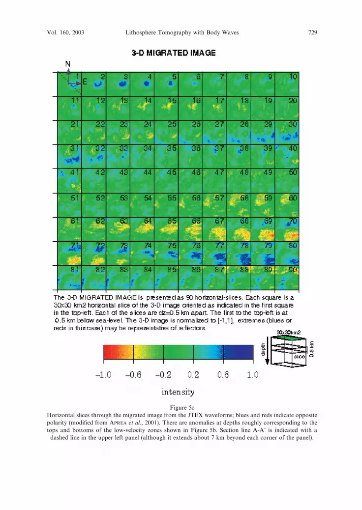
Figure 5c

Horizontal slices through the migrated image from the JTEX waveforms; blues and reds indicate opposite

polarity (modified from APREA et al., 2001). There are anomalies at depths roughly corresponding to the

tops and bottoms of the low-velocity zones shown in Figure 5b. Section line A-A’ is indicated with a

dashed line in the upper left panel (although it extends about 7 km beyond each corner of the panel).


all of which were single-component instruments. The P-wave model that could be

obtained was very coarse, with block size 3� 4� 5 km. The authors were only able

to resolve the top layer adequately, nonetheless they were able to image a zone of low

velocity paralleling the SAF, with higher velocities on either side (Fig. 6a).

The most puzzling finding of the AKI and LEE (1976) study concerned the

earthquake locations. Conventional wisdom held that the SAF is a simple, vertical

strike-slip fault in this area, therefore the epicenters should lie along the fault trace.

However, whether AKI and LEE (1976) started their inversion with hypocenters

aligned on the fault or located several km southwest of the fault, the inversion result

had the earthquakes several km southwest of the fault trace (Fig. 6b). Thus either the

inversion method is flawed or the SAF is unexpectedly complex in Bear Valley. One

possibility is that first-arriving fault zone head waves (BEN-ZION and MALIN, 1991)

may be being modeled as direct waves, resulting in location bias. BEN-ZION et al.

(1992) demonstrate how to use fault zone head waves in an inversion for laterally

heterogeneous fault zone structure.

A recent study of a nearby segment of the SAF (also in the central creeping

section) indicates how much more information can be obtained with a longer-term

Figure 6a

3-D crustal model for the Bear Valley region of central California, showing a low-velocity fault zone

sandwiched between faster basement on either side (modified from AKI and LEE 1976).


deployment of three-component instruments combined with a small active-source

experiment (Fig. 7a). The author’s research group at UW along with Steve

Roecker’s group at RPI and Bill Ellsworth (another Aki student) and co-workers

at the USGS-Menlo Park deployed 50 PASSCAL instruments for 7 months in a

20� 15 km area near Hollister, California, recording hundreds of local

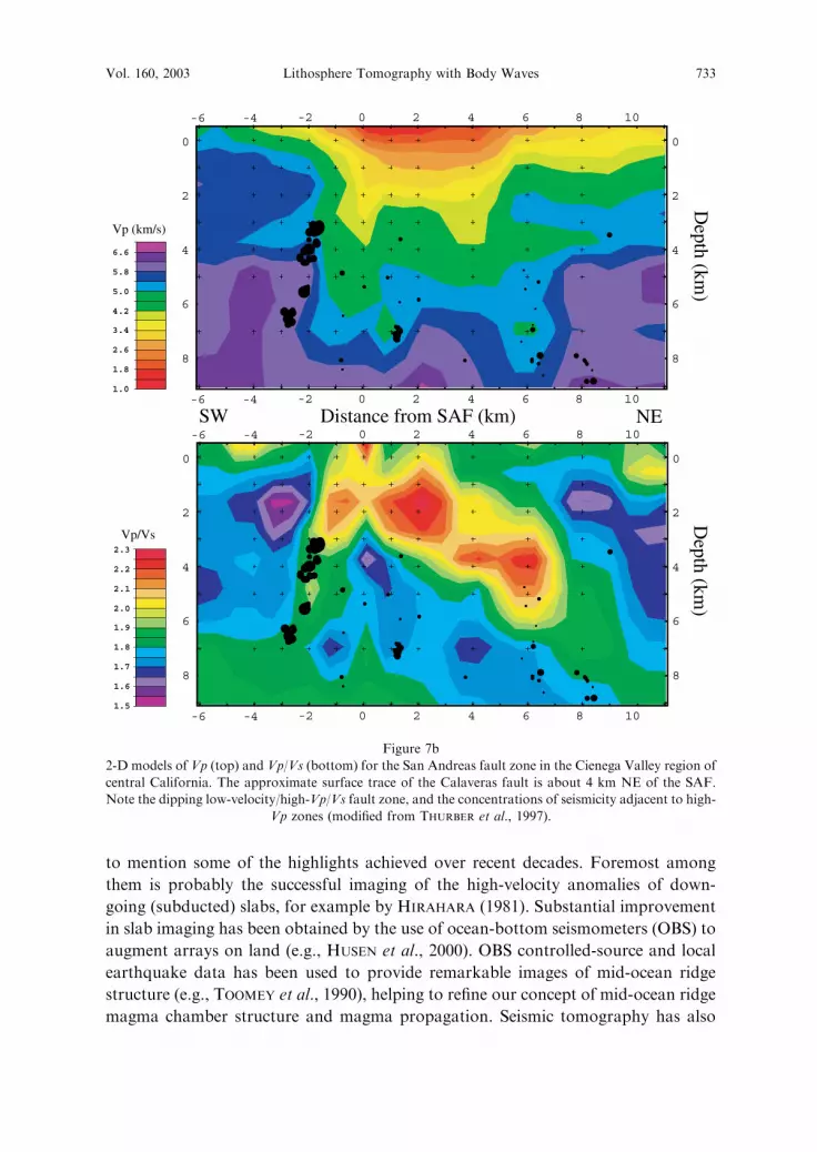
earthquakes (THURBER et al., 1997). Their best resolution was along a 2-D

section normal to the fault, using a grid size as fine as 1 km. Figure 7b shows

their models for Vp and Vp / Vs structure, with seismicity superimposed. They

were able to resolve a deep low Vp and high Vp / Vs anomaly in the fault zone,

Figure 6b

Earthquake relocation results starting from the ‘‘regional’’ (left) and ‘‘local’’ (right) locations (modified

from AKI and LEE 1976). Starting and ending locations are the solid and open circles, respectively. Note

the general agreement in the ending locations for the two different sets of starting locations.


indicative of a highly fractured and probably fluid-rich region. Interestingly, the

P-wave velocity contrasts across the fault are similar between this study and the

original AKI and LEE (1976) study, although they were done along different

sections of the SAF. Note how the seismicity is concentrated on the boundary

between the high and low Vp regions in Fig. 7a, and how regions of high Vp / Vsare virtually aseismic in Fig. 7b. For this section of the SAF, it appears that the

fault dips to the southwest at about 70�.

Other Applications

Although a thorough review of the applications of body-wave seismic tomog-

raphy would require a book (for example, IYER and HIRAHARA (1993)), it is of value

-121˚ 30' -121˚ 24' -121˚ 18' -121˚ 12'

36˚ 33'

36˚ 36'

36˚ 39'

36˚ 42'

36˚ 45'

36˚ 48'

0 5 10

km

San Andreas

Calaveras

Figure 7a

Layout of the seismic array deployed along the San Andreas fault near Hollister in 1994–1995 (modified

from THURBER et al., 1997).


to mention some of the highlights achieved over recent decades. Foremost among

them is probably the successful imaging of the high-velocity anomalies of down-

going (subducted) slabs, for example by HIRAHARA (1981). Substantial improvement

in slab imaging has been obtained by the use of ocean-bottom seismometers (OBS) to

augment arrays on land (e.g., HUSEN et al., 2000). OBS controlled-source and local

earthquake data has been used to provide remarkable images of mid-ocean ridge

structure (e.g., TOOMEY et al., 1990), helping to refine our concept of mid-ocean ridge

magma chamber structure and magma propagation. Seismic tomography has also

8

6

4

2

0

8

6

4

2

0

-6 10 8 6 4 2 0 -2 -4

-6 10 8 6 4 2 0 -2 -4

Vp (km/s)

6.6

5.8

5.0

4.2

3.4

2.6

1.8

1.0

Distance from SAF (km)

Depth (km

)D

epth (km)

Vp/Vs 2.3

2.2

2.1

2.0

1.9

1.8

1.7

1.6

1.5

8

6

4

2

0

8

6

4

2

0

-6 10 8 6 4 2 0 -2 -4

-6 10 8 6 4 2 0 -2 -4

SW NE

Figure 7b

2-D models of Vp (top) and Vp/Vs (bottom) for the San Andreas fault zone in the Cienega Valley region of

central California. The approximate surface trace of the Calaveras fault is about 4 km NE of the SAF.

Note the dipping low-velocity/high-Vp/Vs fault zone, and the concentrations of seismicity adjacent to high-

Vp zones (modified from THURBER et al., 1997).


provided a view of the mantle plume beneath Iceland (WOLFE et al., 1997; ALLEN,

2001). On a global scale, seismic tomography has imaged apparent fossil slabs and

other deep-seated anomalies that likely play a fundamental role in global

geodynamics (VAN DER HILST et al., 1997). Seismic tomography has also been

adapted successfully to surface waves (on local, regional, and global scales), free

oscillations, and attenuation (for body and surface waves). Seismic tomography has

been one of the most widely and successfully used geophysical tools of the past

decade.

Future of Tomography

As we begin the new millennium, there are exciting opportunities for the

application and improvement of seismic tomography. If the proposed Earthscope

program is initiated (HENYEY et al., 2000), seismic tomography will play important

roles in both the USArray and SAFOD components of the program. The plan for the

USArray (LEVANDER et al., 1999; MELTZER et al., 1999) is to deploy 400 broadband

instruments at about 60–70 km spacing, initially in the southwestern United States.

This array would cover about 1/8 of the area of the continental United States at a

time. About a year after the array is fully deployed, it will begin to ‘‘roll’’ around the

continental United States, eventually providing complete, spatially uniform cover-

age. The dataset resulting from this effort will provide an exciting opportunity for the

application of tomography and other imaging and analysis techniques, providing an

unprecedented view of the architecture of the lithosphere beneath the United States.

The plan for SAFOD is to drill a deviated borehole to about 3.5 km depth,

intersecting the SAF in the immediate vicinity of the rupture patches of small

earthquakes. The combination of surface and downhole seismic observations from

SAFOD will permit superb tomographic resolution of the fine structure of an active

fault zone. The author and Steve Roecker deployed a 15-station PASSCAL array in

July 2000, around the proposed drill site for improving earthquake locations, to start

the preparations for drilling at Parkfield.

Acknowledgements

The author is grateful to a number of people and government agencies for advice

and support, respectively, over the last nearly 25 years of my work on seismic

tomography. The list of people starts with Kei Aki, and includes Bill Ellsworth, Steve

Roecker, Donna Eberhart-Phillips, Edi Kissling, Gary Pavlis, Steve Taylor, Bob

Nowack, Bill Prothero, John Evans, Rob Comer, George Zandt, Wim Spakman,

Florian Haslinger, and Stefan Husen. I also thank Florian Haslinger for creating

Figure 1a and for a careful reading of the manuscript. I appreciate the constructive


reviews of Tom Parsons, Donna Eberhart-Phillips, and Associate Editor Yehuda

Ben-Zion. The list of government agencies supporting my tomography research

includes: the National Science Foundation (currently via awards EAR-9814192 and

EAR-9814359), with special thanks to Leonard Johnson; the U.S. Geological Survey

(currently via award 00HQGR0053); and the Defense Threat Reduction Agency

(currently via contract DTRA01-01-C-0085 the content does not necessarily reflect

the position or the policy of the U.S. Government, and no official endorsement

should be inferred). Finally, I thank Jim Fowler and the staff of the IRIS PASSCAL

instrument centers for their dedicated efforts in support of my PASSCAL field

projects over the past decade. The facilities of the IRIS Consortium are supported by

the National Science Foundation under Cooperative Agreement EAR-0004370.

REFERENCES

AKI, K. (1982), Three dimensional Inhomogeneities in the Lithosphere and Asthenosphere: Evidence for

Decoupling in the Lithosphere and Flow in the Asthenosphere, Rev. Geophys. Space Phys. 20, 161–170.

AKI, K., CHRISTOFFERSSON, A., and HUSEBYE, E.S. (1976), Three-dimensional Seismic Structure of the

Lithosphere under Montana LASA, Bull. Seism. Soc. Am. 66, 501–524.

AKI, K., CHRISTOFFERSSON, A., and HUSEBYE, E.S. (1977), Determination of the 3-dimensional Seismic

Structure of the Lithosphere, J. Geophys. Res. 82, 277–296.

AKI, K., and LEE, W.H.K. (1976), Determination of Three-dimensional Anomalies under a Seismic Array

Using First P Arrival Times from Local Earthquakes, 1. A Homogeneous Initial Model, J. Geophys. Res.

81, 4381–4399.

ALLEN, R.M. (2001), The Mantle Plume beneath Iceland and its Interaction with the North-Atlantic Ridge: A

Seismological Investigation, Ph.D. thesis, Princeton University, 184 pp.

APREA, C.M., HILDEBRAND, S., FEHLER, M., STECK, L. BALDRIDGE, W.S., ROBERTS, P., THURBER, C.H.,

and LUTTER, W.J. (2002), 3-D Kirchhoff Migration: Imaging of the Jemez Volcanic Field Using

Teleseismic Data, J. Geophys. Res., in press.

BEN-ZION, Y., KATZ, S., and LEARY, P. (1992), Joint Inversion of Fault Zone Head Waves and Direct P

Arrivals for Crustal Structure near Major Faults, J. Geophys. Res. 97, 1943–1951.

BEN-ZION, Y., and MALIN, P. (1991), San Andreas Fault Zone Head Waves near Parkfield, California,

Science 251, 1592–1594.

BIJWAARD, H., SPAKMAN, W., and ENGDAHL, E.R. (1998), Closing the gap between regional and global

travel time tomography, J. Geophys. Res. 103, 30,055–30,078.

BROCHER, T.M., RUBEL, A.L., WRIGHT, T.L., and OKAYA, D.A. (1998), Compilation of 20 Sonic and

Density Logs from 12 Oil Test Wells along LARSE Lines 1 and 2 in the Los Angeles Basin, California,

U.S. Geol. Surv. Open File Rep. 98-366, 53 pp.

EBERHART-PHILLIPS, D. (1990), Three-dimensional P and S Velocity Structure in the Coalinga Region,

California, J. Geophys. Res. 95, 15,343–15,363.

EBERHART-PHILLIPS, D., LABSON, V.F., STANLEY, W.D., MICHAEL, A.J., and RODRIGUEZ, B.D. (1990),

Preliminary Velocity and Resistivity Models of the Loma Prieta Earthquake Region, Geophys. Res. Lett.

17, 1235–1238.

ELLSWORTH, W.L. (1977), Three-dimensional Structure of the Crust and Mantle beneath the Island of

Hawaii, Ph.D. Thesis, M.I.T. 327 pp.

ENGDAHL, E.R. and LEE, W.H.K. (1976), Relocation of Local Earthquakes by Seismic Ray Tracing,

J. Geophys. Res. 81, 4400–4406.

EVANS, J.R. and ACHAUER, U. (1993), Teleseismic velocity tomography using the ACH method: theory and

application to continental–scale studies. In Seismic Tomography (Iyer, H.M., and Hirahara, K., eds.)

(Chapman and Hall, London, 1993), pp. 319–360.


FOWLER, J. and PAVLIS, G. (1994), PASSCAL; A Facility for Portable Seismological Instrumentation, EOS,

Trans. Am. Geophys. Un. Suppl. 75, 66.

GOMBERG, J.S., SHEDLOCK, K.M., and ROECKER, S.W. (1990), The Effect of S-wave Arrival Times on the

Accuracy of Hypocenter Estimation, Bull. Seismol. Soc. Am. 80, 1605–1628.

HASLINGER, F. and KISSLING, E. (2001), Investigating Effects of 3-D Ray-tracing Methods in Local

Earthquake Tomography, Phys. Earth Plan. Int., in press.

HENYEY, T. and the EARTHSCOPE WORKING GROUP (2000), Earthscope: A Look into our Continent,

Geotimes 45, 5 and 40.

HIRAHARA, K. (1981), Three-dimensional Seismic Structure beneath the Japan Islands and its Tectonic

Implications, J. Phys. Earth 28, 221–241.

HIRAHARA, K. and ISHIKAWA, Y. (1984), Travel-time Inversion for Three-dimensional P-wave Velocity

Anisotropy, J. Phys. Earth 32, 197–218.

HUSEBYE, E.S., CHRISTOFFERSSON, A., AKI K. and POWELL, C. (1976), Preliminary Results of the

3-dimensional Seismic Structure of the Lithosphere under the USGS Central California Seismic Array,

Geophys. J. Roy. Astron. Soc. 46, 319–340.

HUSEN, S., KISSLING, E., and FLUEH, E.R. (2000), Local Earthquake Tomography of Shallow Sudbuction in

North Chile: A Combined Onshore and Offshore Study, J. Geophys. Res. 105, 28,183–28,198.

IYER, H.M. and DAWSON, P.B. (1993), Imaging volcanoes using teleseismic tomography, In Seismic

Tomography, (Iyer, H.M., and Hirahara, K. eds.), (Chapman and Hall, London, 1993), pp. 466–492.

IYER, H.M. and HIRAHARA, K. (eds.), Seismic Tomography (Chapman and Hall, London, 1993), 842 pp.

KISSLING, E. (1988), Geotomography with Local Earthquake data, Rev. Geophys. 26, 659–698.

KISSLING, E., HASLINGER, F., and HUSEN, S. (2001), Model Parameterization in Seismic Tomography: A

Choice of Consequence for the Solution Quality, Phys. Earth Plan. Int., in press.

LEVANDER, A., HUMPHREYS, E., EKSTROM, G., MELTZER, A., and SHEARER, P. (1999), Proposed Project

Would Give Unprecedented Look under North America, EOS, Trans. Am. Geophys. Un. 80, 245, 250–

251.

LUTTER, W.J., FUIS, G.S., THURBER, C.H., and MURPHY, J.R. (1999), Tomographic Images of the Upper

Crust from the Los Angeles Basin to the Mojave Desert: Results from the Los Angeles Region Seismic

Experiment, J. Geophys. Res. 104, 25,543–25,565.

LUTTER, W.J., ROBERTS, P.M., THURBER, C.H., STECK, L.K., FEHLER, M.C., STAFFORD, D.G.,

BALDRIDGE, W.S., and ZEICHERT, T.A. (1995), Teleseismic P–wave Image of Crust and Upper Mantle

Structure beneath the Valles Caldera, New Mexico: Initial Results from the 1993 JTEX Passive Array,

Geophys. Res. Lett. 22, 505–508.

MASSON, F. and TRAMPERT, J. (1997), On ACH, or How Reliable is Regional Teleseismic Delay Time

Tomography?, Phys. Earth Planet. Int. 102, 21–32.

MCCAFFREE, C.L. and CHRISTENSEN, N.I. (1998), Interpretation of Crustal Seismic Velocities in the San

Gabriel-Mojave Region, Southern California, Tectonophysics 286, 252–273.

MELTZER, A., RUDNICK, R., ZEITLER, P., LEVANDER, A., HUMPHREYS, G., KARLSTROM, K., EKSTROM, G.,

CARLSON, C., DIXON, T., GURNIS, M., SHEARER, P., and VAN DER HILST, R. (1999), USArray initiative,

GSA Today 9, 8–10.

MOSER, T.J. (1991), Shortest Path Calculation of Seismic Rays, Geophysics 56, 59–67.

PAVLIS, G.L. and BOOKER, J.R. (1980), The Mixed Discrete Continuous Inverse Problem: Application to the

Simultaneous Determination of Earthquake Hypocenters and Velocity Structure, J. Geophys. Res. 85,

4801–10.

PODVIN, P. and LECOMTE, I. (1991), Finite Difference Computation of Travel Times in Very Contrasted

Velocity Models: A Massively Parallel Approach and its Associated Tools, Geophys. J. Int. 105, 271–284.

PROTHERO, W.A., TAYLOR, W.J., and EICKEMEYER, J.A. (1988), A Fast, Two-point, Three-dimensional

Ray-tracing Algorithm Using a Simple Step Search Method, Bull. Seismol. Soc. Am. 78, 1190–1198.

ROBERTS, P.M., AKI, K., and FEHLER, M.C. (1991), A Low-velocity Zone in the Basement Beneath the

Valles Caldera, New Mexico, J. Geophys. Res. 96, 21,583–21,596.

ROECKER, S.W. (1982), Velocity Structure of the Pamir–Hindu Kush Region: Possible Evidence of Subducted

Crust, J. Geophys. Res. 87, 945–959.

SMITH, S.W. (1986), IRIS: A Program for the Next Decade, EOS, Trans. Am. Geophys. Un. 67, 213–219.


SNIEDER, R. and SAMBRIDGE, M. (1992), Ray Perturbation Theory for Travel Times and Ray Paths in 3-D

Heterogeneous Media, Geophys. J. Int. 109, 294–322.

SPENCER, C. and GUBBINS, D. (1980), Travel-time Inversion for Simultaneous Earthquake Location and

Velocity Structure Determination in Laterally Varying Media, Geophys. J. R. Astron. Soc. 63, 95–116.

STECK, L., THURBER, C., FEHLER, M., LUTTER, W., ROBERTS, P., BALDRIDGE, S., STAFFORD, D., and

SESSIONS, R. (1998), Crust and Upper Mantle P-wave Velocity Structure Beneath the Valles Caldera, New

Mexico: Results from the JTEX Teleseismic Experiment, J. Geophys. Res. 103, 24,301–24,320.

THURBER, C.H. (1981), Earth Structure and Earthquake Locations in the Coyote Lake Area, Central

California, Ph.D. Thesis, M.I.T. 331 pp.

THURBER, C.H. (1986), Analysis Methods for Kinematic Data from Local Earthquakes, Rev. Geophys. 24,

793–805.

THURBER, C.H. (1992), Hypocenter-velocity Structure Coupling in Local Earthquake Tomography, Phys.

Earth Planet. Int. 75, 55–62.

THURBER, C.H. and ELLSWORTH, W.L. (1980), Rapid Solution of Ray-tracing Problems in Heterogeneous

Media, Bull. Seismol. Soc. Am. 70, 1137–48.

THURBER, C.H. and KISSLING, E., Advances in travel-time calculations for three-dimensional structures. In

Advances in Seismic Event Location, (Thurber, C., and Rabinowitz, N., eds.), (Kluwer Academic

Publishers, Dordrecht, Netherlands 2000) pp. 71–99.

THURBER, C., ROECKER, S., ELLSWORTH, W., CHEN, Y., LUTTER, W., and SESSIONS, R. (1997), Two-

dimensional Seismic Image of the San Andreas Fault in the Northern Gabilan Range, Central California:

Evidence for Fluids in the Fault Zone, Geophys. Res. Lett. 24, 1591–1594.

TOOMEY, D.R., PURDY, G.M., SOLOMON, S.C., and WILCOCK, W.S.D. (1990), The Three-dimensional

Seismic Velocity Structure of the East Pacific Rise near Latitude 9� 30’ N, Nature 347, 639–645.UM, J. and THURBER, C.H. (1987), A Fast Algorithm for Two-point Seismic Ray Tracing, Bull. Seismol.

Soc. Am. 77, 972–986.

VAN DER HILST, R.D., WIDIYANTORO, S., and ENGDAHL, E.R. (1997), Evidence for Deep Mantle Circulation

from Global Tomography, Nature 386, 578–584.

VIDALE, J.E. (1988), Finite-difference Travel-Time Calculation, Bull. Seis. Soc. Am. 78, 2062–2076.

VIDALE, J.E. (1990), Finite-difference Calculation of Travel Times in Three Dimensions, Geophysics 55, 521–

526.

VIRIEUX, J., FARRA, V., and MADARIAGA, R. (1988), Ray Tracing for Earthquake Location in Laterally

Heterogeneous Media, J. Geophys. Res. 93, 6585–6599.

WIDIYANTORO, S., and VAN DER HILST, R. (1997),Mantle Structure beneath Indonesia Inferred from High-

resolution Tomographic Imaging, Geophys. J. Int. 130, 167–182.

WOLFE, C.J., BJARNASON, I.T., VAN DECAR, J.C., and SOLOMON, S.C. (1997), Seismic Structure of the

Iceland Mantle Plume, Nature, 385, 245–247.

ZHAO, D., HASEGAWA, A., and HORIUCHI, S. (1992), Tomographic Imaging of P- and S- wave Velocity

Structure beneath Northeastern Japan, J. Geophys. Res. 97, 19,909–19,928.

(Received July 1, 2000, accepted January 31, 2001)

To access this journal online:

http://www.birkhauser.ch


Seismic Tomography of the Lithosphere with Body Waves

Documents

Transcript of Seismic Tomography of the Lithosphere with Body Waves