Report of the ICES-FAO Working Group on Fishing ... - Archimer
Upload
khangminh22Category
view
1download
0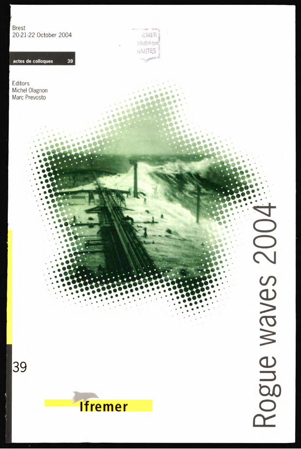
Brest 20-21-22 October 2004
actes de colloques 39
Editors Michel Olagnon Marc Prevosto
39
Ifremer Rogu
e w
aves
200
4

ZL c>3o
Rogue Waves 2004 Michel Olagnon & Marc Prevosto Editors
Proceedings of a Workshop organized by Ifremer and held in Brest, France 20-21-22 October 2004 within the Brest Sea Tech Week 2004
See also http://www.ifremer.fr/web-com/stw2004/rw/
Ifremer

I
Preface
Every four years, athletes meet at the Olympic games in a friendly competition to raise their performances to higher levels than ever, probably because such a four year duration is the right time interval for efforts to mature into significant progress. Four years after the Rogue Waves 2000 workshop, we thus decided to hold a second Rogue Waves workshop, gathering again researchers, forecasters and industry people to strengthen their work by exchanges in and around a conference room.
We have been very pleased that many of them did respond with evidence of high-quality work carried out since they had gone home after the first workshop. The aim of this second workshop was to assess the state of the art as to conditions of occurrence of waves or groups of waves of unexpected severity, responsible for ship wrecks and damage to offshore oil and gas production systems; and to establish a “road map” as to research actions and collaborations needed to improve the prediction and forecasting abilities in this domain.
We organized the sessions in three groups:
1. Definition, characterization and discussion of the rogueness of waves from their statistics and from the manners in which they affect ships and ocean structures.
2. Generating mecanisms for rogue waves, validation from numerical and physi-cal experiments, observation and comparison between observed and modelled features.
3. Prediction of rogue waves in the short term, through warnings issued with sea conditions forecasts, and in the long term as refinements in the metocean climate descriptions and in the design procedures. What problems are rogue waves facing us with ?
A discussion moderated by Michel Huther concluded the workshop. It stressed that target levels of safety are probably not in jeopardy when global design is considered, but that the problem of how to avoid being caught at the wrong time in the wrong place is still far from being solved.
So we hope to to be able to gather participants again in 2008 to discuss their progress on those issues, and may their findings be such that all sailors and workers at sea know afterwards how to keep themselves safe from rogue waves !
September 2005 Michel Olagnon & Marc Prevosto editors of the proceedings
ROGUE WAVES 2004

II
Organization
ROGUE WAVES 2004 was organized by the Hydrodynamics and Met,ocean Group of Ifremer (Institut Français de Recherche pour l’Exploitation de la Mer) and benefîtted from the support of the Communauté Urbaine de Brest (now Brest Métropole Océane) and of the Région Bretagne.
It was one of the events of the Brest SeaTechWeek 2004, a week devoted to exchanges between research and industry in marine science and technology.
Our thanks go to all those who supported this workshop by helping finding funding and volunteering their personal time and efforts.
Participants
Pierre Ailliot email [email protected] Bertrand Alessandrini email [email protected] Fabrice Ardhuin email [email protected] Gerassimos Athanassoulis email [email protected] Rolf Baarholm email [email protected] Sergei Badulin email [email protected] Nigel Barltrop email [email protected] Anne Barthélémy email [email protected] Elzbieta Bitner-Gregersen email [email protected] Félicien Bonnefoy email [email protected] Bas Buchner email [email protected] Alexander Bukhanovsky email [email protected] David J.T. Carter email [email protected] Luigi Cavaleri email [email protected] Lennart Cederberg email [email protected] Arnaud Coatanhay email [email protected] Edmond Coche email [email protected] Gilbert Damy email [email protected] Frédéric Dias email [email protected] Mark Donelan ('mail [email protected] Kristian Dysthe ((mail [email protected] Kenneth Johannessen Elk email [email protected] Pierre Ferrant email [email protected] Cyril Frelin email [email protected] Dorian Fructus email [email protected] Richard Gibson email [email protected] E.Brenny van Groesen email [email protected] John Grue email [email protected] Johannes Guddal email [email protected] Carlos Guedes Soares email [email protected]

Ill
Gil-Yong Han email [email protected] Frédéric Hauville email [email protected] Sverre Haver email [email protected] Martin Holt email [email protected] Michel Hontarrede email [email protected] Erlend Hovland email [email protected] René Huijsmans email [email protected] Keith MacHutchon email [email protected] Michel Huther email [email protected] Alastair Jenkins email [email protected] Lars Johansson email [email protected] Natanael Karjanto email [email protected] Christian Kharif email kharif «mousson.irphe.univ-mrs.fr Olivier Kimmoun email [email protected] Gert Klopman email [email protected] Harald E. Krogstad email [email protected] Marc Le Boulluec email [email protected] Georg Lindgren email [email protected] Paul C Liu email [email protected] Leonid Lopatoukhin email [email protected] Anne Karin Magnusson email [email protected] Christophe Maisondieu email [email protected] Gianluca Manes email [email protected] Bernard Molin email [email protected] Valérie Monbet email [email protected] Nobuhito Mori email [email protected] Alan Murphy email [email protected] Guillaume Oger email [email protected] Michel Olagnon email [email protected] Miguel Onorato email [email protected] Efim Pelinovsky email [email protected] D.Howell Peregrine email [email protected] Marc Prevosto email [email protected] Igor Rychlik email [email protected] Henri Savina email [email protected] Chris Shaw email [email protected] Hervé Socquet-Juglard email [email protected] Tarmo Soomere email [email protected] Christopher Swan email [email protected] Paul Taylor email [email protected] Rodolfo Tedeschi email [email protected] Alessandro Toffoli email [email protected] Hiroshi Tomita email [email protected] Karsten Trulsen email [email protected] Arnaud Vazeille email [email protected] Arjan Voogt email [email protected]

IV
Contents
Definition, characterization and discussion of the rogueness of waves from their statistics and from the manners in which they affect ships and ocean structures.
Session 1.1: Large ships and platforms (life-long extremes)
Introductory presentation:
- Sverre Haver (Statoil, Norway) - Freak Waves - A Suggested Definition and Possible Consequences for Marine Structures
Regular presentations:
- Bas Buchner and Arjan Voogt (Marin, The Netherlands) - Wave impacts due to steep fronted waves
- Rolf Baarholm and Carl Trygve Stansberg (MARINTEK, Norway) - Ex-treme Wave Impact on GBS Platform Deck
- D.Howell Peregrine (School of Mathematics, Bristol University, UK) - (Ab-stract) Violent water wave impacts on a wall
- Nigel Barltrop (Universities of Glasgow and Strathclyde, UK) - (Abstract) A simple wave front steepness enhancement prediction methodology
- Bernard Molin, F. Remy, 0. Kimmoun, E. Jamois (EGIM, France) - (Ab-stract) Enhanced wave effects on the weather side of reflective structures
- Anne Karin Magnusson (Met.no, Norway), Jaak Monbaliu, Alessandro Tof-foli (KU Leuwen, Belgium) and Elzbieta Bitner-Gregersen (DNV, Norway) - (Abstract) On the shape of large waves in the central and southern North Sea
- Paul C. Liu (NOAA, USA), Keith MacHutchon (Liebenberg & Slander Inter-national, South Africa) Exploring rogue waves from observations in South Indian Ocean
Session 1.2: Small crafts, high speed crafts (unexpected highs in operational conditions)
Introductory presentation:
- Bruce Johnson (US Naval Academy, USA) and Stefan Grochowalski (Ot-tawa, Canada) - (Abstract - paper not presented due to last minute problem) Development of Operational Guidance Criteria for Small Craft Operating in Dangerous Seas
Regular presentation:
- Soren Peter Kjeldsen (Trondheim Maritime Academy, Norway) - Examples of observed freak waves in Norway and related ship accidents (Paper not presented due to last minute problem).

V
Generating mecanisms for rogue waves, validation from numerical and physical experiments, observation and comparison between observed and modelled fea-tures.
Session 2.1: Theoretical results, numerical and physical simulations
Introductory presentation:
- Paul H. Taylor (University of Oxford, UK) - (Abstract) Rogue Waves and wave focusing - speculations on theory, numerical results and observations
Regular presentations:
- Richard Gibson and Chris Swan (Imperial College London, UK) - The role of resonant wave interactions in the evolution of extreme wave events.
- J.P. Giovanangeli, C. Kharif (IRPHE, France) and E. Pelinovsky (Institute of Applied Physics, Nizhny Novgorod, Russia) - Experimental study of the wind effect on the focusing of transient wave groups
- Dorian Fructus and John Grue (Universitetet i Oslo, Norway) - A rapid fully nonlinear method in three dimensions with simulations of steep wave event
- J. Grue, D. Clamond, M. Francius (Universitetet i Oslo, Norway) and C. Kharif (IRPHE, France) - On the role of downshifting in formation of large wave events
- Tarmo Soomere and Jiiri Engelbrecht (Tallinn Technical University, Esto-nia) - Extreme elevations and slopes of interacting Kadomtsev-Petviashvili solitons in shallow water
- Hervé Socquet-Juglard, Kristian Dysthe (Universitetet i Bergen, Norway), Karsten Trulsen (Matematisk Institutt, Universitetet i Oslo, Norway), Har-ald E. Krogstad, Jingdong Liu (NTNU, Trondheim, Norway) - (Abstract) Distribution of extreme waves by simulations
- Félicien Bonnefoy, Pierre Roux de Reilhac, David Le Touzé, Pierre Ferrant (Ecole Centrale de Nantes, France) - Numerical & Physical Experiments of Wave focusing in short-crested seas
- Karsten Trulsen (Maternatisk Institutt, Universitetet i Oslo, Norway) - (Ab-stract) Transversal crest and group modulation of extreme waves
- C. Fochesato, F. Dias (ENS Cachan, France), S. Grilli (University of Rhode Island, USA) - Wave energy focusing in a three-dimensional numerical wave tank
- Miguel Onorato, Alfred Osborne, Marina Serio (University of Torino, Italy) Quasi-resonant interactions and non-Gaussian statistics in long-crested
waves - Guillaume Oger, Mathieu Doring, Bertrand Alessandrini, Pierre Ferrant
(Ecole Centrale de Nantes, France) - SPH: Towards the simulation of wave-body interactions in extreme seas

VI
- Sergei Badulin (Russian Academy of Sciences, Moscow, Russia), A. Pushkarev (Waves and Solitons LLC, USA), D. Resio (US Army Engineer R&D Center, USA), V. Zakharov (Russian Academy of Sciences, Moscow, Russia & Uni-versity of Arizona, USA) - Self-similarity of wind-wave, spectra. Numerical and theoretical studies
Session 2.2: Comparison with observed results
- Hervé Soequet-Juglard and Kristian B. Dysthe (University of Bergen, Nor-way), Karsten Trulsen (University of Oslo, Norway), Sébastien Fouques, Jingdong Liu and Harald E. Krogstad (NTNU, Trondheim, Norway) - Spa-tial extremes, shapes of large waves and, Lagrangian models Chris Swan, Richard Gibson and Peter Tromans (Imperial College London, UK) Wave crest statistics calculated using a fully nonlinear spectral re-sponse surface method Andonowati and E. van Groesen (Marin, The Netherlands) Deterministic Aspects of Nonlinear Modulation Instability Nobuhito Mori, (Osaka City University, Japan) and Peter A.E.M. Janssen (ECMWF, UK) Dependence of freak wave occurrence on kurtosis
- Elzbieta Bitner-Gregersen (DNV, Norway) & Anne Karin Magnusson (Met.no, Norway) - Extreme Events in Field Data and in a Second Order Wave Model
- Michel Olagnon (Ifremer, France) & Anne Karin Magnusson (Met.no, Nor-way ) — Spectral parameters to characterize the risk of rogue waves occurrence in a sea state R. Huijsmans, N. Karjanto, Andonowati, Klopman & E. van Groesen (Marin, The Netherlands) - Experiments on extreme wave generation using the Soli-ton on Finite background
- Alastair D. Jenkins (Universitetet i Bergen, Norway), Anne Karin Magnus-son (Met.no, Norway), Andreas Niedermeier (DLR, Germany), Jaak Mon-baliu and Alessandro Toffoli (KU Leuwen, Belgium), Karsten Trulsen (Matem-atisk Institutt, Universitetet i Oslo, Norway) — Rogue waves and extreme events in measured time-series
- C. Guedes Soares, and E.M. Antâo (IST, Portugal) - Comparison of the characteristics of abnormal waves on the North Sea and Gulf of Mexico

VII
Prediction of rogue waves in the short term, through warnings issued with sea
conditions forecasts, and in the long term as refinements in the metocean climate descriptions and in the design procedures.
Session 3.1: Can sensible warnings be issued ?
Introductory presentation:
- Henri Savina & Jean-Michel Lefèvre (MétéoFrance) Sea state in Marine Safety Information : present state, future prospect (Oral Presentation only)
Regular presentations:
- Martin Holt, Gary Fullerton, Jian-Guo Li (Met Office, UK) - Forecasting sea state with a spectral wave model (Oral Presentation only)
- A.V.Boukhanovsky (Institute for High Performance Computing), L.J.Lopatoukhin (State University, Dep. Oceanology) (St. Petersburg, Russia) and C.G.Soares (Instituto Superior Tecnico, Lisboa, Portugal) Climatic wave spectra and freak waves probability
- Mark A. Donelan (university of Miami/RSMAS, USA), Anne Karin Mag-nusson (Met.no, Norway) and Elzbieta Bitner-Gregersen (DNV, Norway) Towards a Global Rogue Wave Warning System (Oral Presentation only)
Session 3.2: Should we modify design specifications ?
Introductory presentation:
- Gil-Yong Han (IACS - International Association of Classification Societies) - Ship design rules and regulations, an overview of major themes
Regular presentations:
- C. Guedes Soares, N. Fonseca and R. Pascoal (IST, Portugal) - Comparison of present wave induced load criteria with loads induced by an abnormal wave on marine structures

VIII
Our warmest thanks to Professor Laurence Draper and to David Charter for pro-viding reprints of the first known articles about freak waves, to an anonymous former cadet of the Jeanne d’Arc for the report of a near-miss, and to Sverre Haver for clarifying the story of the famous “New Year Wave”.
Historical reprints
- Laurence Draper (reprinted from Oceanus (X:4), July 1964) - “Freak” Ocean Waves Laurence Draper (reprinted from J. Navigation (24:3), Royal Inst. of Navi-gation , July 1971) - Severe Wave Conditions at Sea
Testimonies
- Cdt. Frédéric-Moreau (Jeanne d’Arc, France) The Glorious Three Sverre Haver (Statoil, Norway) A possible freak wave event measured at the Draupner Jacket January 1, 1995

Freak Waves: A Suggested Definition and Possible
Consequences for Marine Structures
Sverre Haver
Marine Structures and Risers, Statoil ASA, N-4035 Stavanger, Norway [email protected]
Abstract. Target annual exceedance probabilities of design loads of offshore structures on the Norwegian Continental shelf are briefly discussed. It is proposed to define freak wave events as events that are well beyond what is typically expected within wave theories utilized for structural design. With this background, the question of whether or not freak waves are of concern for practical design work is discussed. The discussion is not conclusive, and major focus is given to some questions that need to be properly answered before a final conclusion can be made.
1 Introduction
This paper is prepared as an introductory lecture to a session discussing rogue waves and practical problems related to their possible existence. The paper do not present any new evidences of freak waves. The purpose is merely to present some few questions that need to be properly answered before it can be concluded whether or not freak waves represent a threat to structural integrity. Hopefully, these questions and accompanied discussions can act stimulating on those research groups addressing freak waves from a more basic research point of view.
Offshore structures at the Norwegian Continental Shelf are with respect to overload designed against environmental loads corresponding to an annual exceedance probability of 10-2 multiplyed by a partial load factor of 1.3, Norsok(1999). Provided that the load versus exceedance probability is of a well behaved nature, the design load thus obtained is tacitly assumed to result in a reasonable platform safety against collapse. However, this may not be the case if for some reason the load – exceedance probability relation changes abruptly in a worsening direction for exceedance probabilities between 10-2 and 10-4. Such an abrupt change in load pattern could take place if the most extreme waves impact the deck structure. An illustration of the load – exceedance probability relation for a well behaving and a bad behaving response problem is shown in Fig. 1. In order to ensure that an ill behaving response problem is not slipping unnoticed through the design process, Norwegian Offshore Regulations, NPD(2001), also

requires that the structures shall withstand 10-4-probability1 environmental loads with at most some local damage. There is not a one-to-one relation between wave crest height and platform loading, but in most cases there is a rather large positive correlation. This means that if we shall be able to predict reasonable estimates for the q-probability loads, q=10-2 and 10-4, the wave models used for design should accurately reflect wave events with occurrence probabilities of the order of magnitudes. Accordingly, a quantity of crucial concern is the very upper tail of the annual distribution function of wave events and loads, i.e. annual exceedance probabilities in the range 10-2 – 10-5. Provided that the sea surface can be modeled as a stationary and homogeneous second order random field, see e.g. Marthinsen and Winterstein (1992), Forristall (2000), it is expected that it is possible to estimate the upper tail of the annual extreme value distributions with a sufficient accuracy. The challenging question, however, is whether or not there exists wave phenomena beyond our adopted design model which may affect the very upper tails significantly.
0 1 2 3 4 5
- log(annual exceedance probability)
sc,ULS
1.3*sc,ULS
Load-level
Well-behaving problem
Bad-behaving problem
sc,ALS,1
sc,ALS,2
Fig. 1. Illustration of well-behaving and bad-behaving response problem.
2 Are rogue waves a problem for structural design?
The answer to this question depends very much on what is meant by a rogue wave. There is at least two options: i) “Classical” extreme waves and ii) Freak extreme waves. Unfortunately, it is not always clear what people mean when they refer to rogues waves. As an extended introduction, some paragraphs will therefore be spend on clarifying what will be meant throughout this paper.
1 Q-probability event means an event corresponding to an annual exceedance probability of q.

”Classical” extreme waves By classical extreme waves, we will herein think of rare members of a population of wave events defined by modeling the surface process as a piecewise stationary and homogeneous slightly non-Gaussian random field. The word “classical” is introduced since this approach is what in principle is available for routine design. Over the years, the so-called “classical” population has evolved somewhat. One to two decades ago, the surface process was often modeled as Gaussian random field. As a consequence of that the “classical” extreme crest height population of those days was shifted slightly to smaller values than those being in agreement with the present definition. This type of extreme waves are in most cases properly accounted for by the offshore industry, provided some 10-4 – probability wave load scenario is implemented. Traditional shipping may have some room for improvements both when it comes to the implementation of a slightly non-Gaussian surface process and the adopted exceedance probabilities for the design loads. The latter is in particular the case when it comes to slamming and green water related problems. It is important to realize that even within “classical” extreme waves population, wave events which may represent a threat to the integrity of a structure do exist. However, their annual exceedance probability for a given site should be lower than say 10-5 if a structure is properly designed. Freak ( extreme) waves Herein we will define freak waves as typical members of population being defined by physical mechanisms well beyond those underlying “classical” extreme waves. These types of extreme wave events are not explicitly accounted for in the design process. If such a population exists, it may challenge present design recipes if it significantly affects wave properties (crest heights, wave heights, wave steepness) at a given site corresponding to annual exceedance probabilities of 10-3 – 10-5 . It should be noted that we throughout this paper always will refer to the annual extreme value distribution functions at a given site. This because a structure can not simultaneously sample wave events more than at one site. The rule requirements to target maximum exceedance probability of the design loads, therefore refer to annual exceedance probabilities at a particular site. In case of traditional shipping, this site would be a site moving along a given route. Which out of these populations is the most common adopted definition of rogue waves is hard to say. It seems as if the rogue waves population often is meant to capture both populations referred to above. From a practical point of view that is not convenient, because a major part of the rogue wave population, “classical” extreme waves, does not represent a problem, while the freak extreme waves population, if it exists, may represent a challenge.

3 Suggested definition of freak waves
The most common definition of a freak wave, is to define a wave as a freak wave if the wave height to significant wave height ratio or the crest height to significant wave height ratio exceed some thresholds. A factor definition may be useful as a first indicator of possible freak event. In this connection, the recommended thresholds should account for the duration of the observation window, i.e. is the observed maximum a 20-min. maximum, is it a 3-hour maximum or is it a storm maximum. From a practical point of view it seems more convenient to anchor the definition of a freak wave to mechanisms not captured by the wave models used for design purposes. It is therefore recommended to define freak waves as follows, Haver (2000): A freak wave event is an event (crest height, wave height, steepness or group of waves) that represent an outlier when seen in view of the population of events generated by a piecewise stationary and homogeneous second order model of the surface process. The definition is related to major deviations from a second order model because this is the most sophisticated model that is available for routine design work. As more sophisticated model for design is developed, the “classical” extreme wave population will grow on the cost of the freak wave population. If one is to look for freak waves in available measurements, one will need a freak wave indicator as the observations are scanned. For such a purpose a factor threshold is useful. If we are basing the data search on scanning of 20-min. time series, one should establish proper threshold for this experiment. If the sea surface is modeled as a second order process, the 99-percentile of the ratios shc /.min20− and shh /.min20− read about 1.25 and 2.00, respectively, Haver(2000). If an observation exceeds this threshold, one may at a significance level of 1% reject this observation as a realization from a second order process of 20-min. duration. However, further investigations should be carried out before the event is concluded as belonging to the freak extreme waves population. If the observation window is increased to 3-hours, more adequate thresholds would be 1.50 and 2.45, respectively. If a storm is defining the observation window, 1.60 and 2.55 will probably represent adequate thresholds if a 1% significance level is found proper for the freak wave indicator. The advantage of this definition is that we accept that rather lather freak wave indicator factors occur even within the “classical” extreme waves population. If a separate phenomenon can be excluded, freak wave should be of no concern. If a structure is being hit by an unexpectedly large wave event, it is then merely a matter of being at the wrong place at the wrong time. The annual occurrence probability of this event, however, should be well below the target annual exceedance probabilities of the design loads.

Finally, it should be pointed out that the thresholds recommended above, refer to observations from a given site. If the observation window is extended to also cover spatial domain, the thresholds for the indicator should be significantly increased in order to account for effects discussed by Krogstad et al. (2004).
4 Why should we be concerned about freak waves?
It is seen from Fig. 1 that an ill-behaving response problem being overlooked in the design process could represent a threat to the structural integrity. The figure reflects the airgap problem. In practice this problem is dealt with by requiring that the airgap is sufficiently large for the annual wave-deck impact probability to be less than 10-4.In this connection, the 10-4 crest height is estimated using the classical extreme wave population. If a freak wave population exists and if it is realized sufficiently frequent to effect the interesting part of the annual extreme value distribution of the crest height, freak waves may represent a source for an ill-behaving response problem, i.e. a scenario where for a low exceedance probability the load increases abruptly. This is because a fatter tail will make a wave-deck impact more probable. The possible effect of freak waves which we should be concerned about is illustrated in Fig. 2. If a freak wave population exists, what is the problem? For ships and offshore platforms, a freak wave will mainly represent a problem if its crest hits structural members which is not designed for wave loads. As far as no new members are exposed, the global loading due to a freak wave is most probably smaller than the global loading in connection with a “classical” extreme wave. However, it is recommended that further work are carried out in order to establish some documented knowledge on the freak wave kinematics.
Annual maximum crest height
Cum
ulat
ive
prob
abili
ty–
Gum
bels
cale
Gaussian sea
Second order sea
Fully non-linear sea
Possible effect ofthe freak phenomenon10-3
10-5
Fig. 2. Possible effect of freak waves of annual extreme value distribution of wave crest height

5 The freak wave challenge
With respect to waves, offshore structures are designed against the q-probability waves from the population referred to herein as the “classical” extreme waves. If the design process also involves a proper check of the structure against accidental waves (10-4 – probability waves), a certain robustness against freak wave events is achieved. This is under the assumption that it is not the group involving the worst waves from the “classical” extreme waves that is focused into a single majestic wave. However, if this assumption is not true, freak waves may, if they exist as a separate phenomenon, represent an unknown or unquantified threat to marine structures. At present it is not possible to approach freak waves in a rational way in the design process. In order to be able to account for possible freak waves in rational design recipe, the following questions need to be answered:
• Does a separate freak wave population exist? One needs to identify the underlying physical mechanisms that can make a freak wave development possible.
• Given a separate population exists, what is the conditional probability, say per 3-hour duration of a sea state, for a freak wave development given some engineering sea state characteristics? From a design point of view, a freak wave does not represent a problem unless it at a given site occurs sufficiently frequent to effect our predictions of 10-2 - and 10-4 – probability wave events.
• Given a freak wave occurs in a 3-hour sea state with given characteristics, what is the conditional distribution for the freak wave amplification factor? The freak wave amplification factor is defined as the ratio
nonfreakhfreakhr cc ,3,3 / . In some cases a freak wave will not be larger than the largest wave in another group of the sea state not being exposed to a freak wave development. On the other hand, if it is the largest group of the sea states that developes into a single majestic wave, the amplification factor may be considerable.
Wave data collection programs will possibly not be the most adequate approach for concluding on the existence of a separate freak wave population. In case of an unexpectedly large observation, one will face the following question, Haver and Andersen (2000): Is the observed wave a very rare realization from the typical slightly non-Gaussian sea surface population, or, is it a typical realization of a very rare and strongly non-Gaussian sea surface population? A more fruitful approach in the long run is to develop mathematical models accounting properly for the underlying physics including the physics that may govern a freak wave development. If such a model becomes available, one should in principle be able to answer the two last equations through time domain simulations of sea surface fields. A rather qualitative assessment of whether or not freak waves represent a problem for practical design was presented by Haver et al. (2004). The basic idea of that

assessment is that we for any sea state can establish a proper extreme value distribution for C3hr,nonfreak , i.e. the 3-hour maximum crest height given no freak wave development took place. The conditional probability of freak wave development is measured by a two outcome variable, K. If no freak wave development take place, K=0, while K=1 describes a freak wave development. At present we do not know the conditional probability of K=1 for the various sea states and in the paper it is simply modeled as a bell shape function of hs and tp. An example of P(K=1 | Hs, Tp) is shown in Fig. 3. In the study some sensitivity studies of the parameters of this function are included. The 3-hour maximum accounting for a possible freak wave development is written on the following form:
C3hr,freak = C3hr, nonfreak + K*∆C3h,freak = C3hr, nonfreak(1 + K*Λ) (1)
∆C3h,freak is the increase of the 3-hour maximum crest height due to the freak wave development. Λ describes the same quantity normalized by the 3-hour maximum if no freak wave development takes place. Λ = 0 if the freak wave crest height is not the highest crest height of the sea state. This is more or less arbitrarily assumed to be the case in 25% of the cases with a freak wave development. The distribution function for Λ is shown in Fig. 4. The qualitative study indicates that if the chance of a freak wave development is very small, which is what available observations suggest, freak waves will not affect design wave events. However, one has to keep in mind that most of our observations correspond to sea states not much more severe than what the 1- to 10-year contour lines shown in Fig. 5 suggest. However, a wave event is not expected to be critical regarding structural integrity before we approach or exceed the 10000-contour of Fig. 5. If the conditional probability of K=1 is much higher for sea states beyond what are presently observed, freak waves may represent a threat to marine structures. It is therefore recommended that research is continued until it can with reasonable confidence conclude that the freak wave probability is not positively correlated with sea state severity. Severity is in this connection not measured only in significant wave height.
6 Possible mechanisms for a freak wave development
Herein we will not review the various mechanisms that have been proposed as possible freak wave mechanisms. The reader could review other presentations at this workshop or consult proceedings from the previous rogue waves work shop, Olagnon and Athanassoulis (2001). One of the mechanisms, Benjamin-Feir instability, seems to require that surface process need to be rather narrow banded both frequency (wave number) and direction in order to be realized. The real ocean surface is typically short crested suggesting that the real sea surface is less exposed to the self focusing of major wave groups. However, the real ocean is not homogeneous and stationary to the extent that is typically utilized in ocean engineering. Fig. 6 shows an illustration of a

sea surface that is generally of a short crested nature, but where a sub-area is assumed to exist. Is this a possible scenario in the real world? Are we smoothing away these possibilities by our input assumption of piecewise homogenity and stationarity? One should probably approach these questions rather open minded although if these assumptions have to be skipped, the ergodicity assumption that is underlying much of our work in ocean engineering can be questioned. Satellite observations of larger areas may prove very useful when it comes to verify our assumption of sea surface homogeneity.
0.5
3.5
6.5
9.5
12.5
15.5
18.5
21.5
24.5
27.5
30.5
0.52.54.56.58.510.512.514.516.518.5
Spectral Peak Period (s)
Significant Wave H
eight (m)
Freak Wave Event Probability psimax=0.025, h0=12m, t0=12s
0.02-0.025
0.015-0.02
0.01-0.015
0.005-0.01
0-0.005
Fig. 3. Illustrative conditional probability of freak wave phenomenon given sea state characteristics.
0
0.2
0.4
0.6
0.8
1
1.2
0 0.5 1 1.5 2 2.5
lambda
Cum
ulat
ive
Prob
abili
ty
Fig. 4. Illustrative conditional distribution function of the freak wave development factor.

Fig. 5. q-probability contour lines for Hs and Tp for a Northern North Sea location
Offshore structure
Fig. 6. Illustration of a short crested sea surface with a long crested sub-domain.
7 Conclusions
The discussions presented previously can be summarized as follows:
• Freak waves should be defined as a separate population well beyond the population used for design purposes.
• Freak waves are not likely to represent a problem for offshore structures if their frequency of occurrence experienced for the sea states observed so far is generally valid.
• There is some concern that traditional ships may experience considerable damages in extreme wave conditions, even if the waves are well within the classical extreme wave population.
• Freak waves may be of some concern if their conditional occurrence probability is increasing as we enter into the range of non-observed sea state severities.

• A first step to gain some robustness against unknown freak wave extremes, could be to involve an accidental wave event (10-4 – probability wave event) into the design process.
8 Acknowledgement
Statoil ASA is acknowledged for the permission to publish this paper. It should be pointed out the views presented herein are those of the author and should not be construed as necessarily reflecting the views of Statoil.
9 References
Forristall, G.Z. (2000): “Wave Crest Distribution: Observations and Second-Order Theory”, Journal of Physical Oceanography, Vol. 30, August 2000. Olagnon, M. and Athanassoulis, G.A. (2001) (Editors): “Rogue Waves 2000”, Proceedings of a Workshop organized by Ifremer, November 29-30, Brest France. Haver, S. and Andersen, O.J. (2000): “Freak Waves: Rare Realizations of a Typical Population or Typical Realizations of a Rare Population?”, ISOPE-2000, May 2000, Seattle, USA. Haver, S. (2000): “Evidences on the Existence of Freak waves”, Rogue Waves 2000, November 2000, Brest France.
Haver, S., Vestbøstad, T. M., Andersen, O. J. and Jakobsen, J.B. (2004): “Freak Waves and Their Conditional Probability Problem”, ISOPE 2004, May 2004, Toulon, France. Krogstad. H., Liu, J., Socquet-Jugland, H., Dysthe, K.B. and Trulsen, K. (2004): “Spatial extreme value analysis of nonlinear simulations of random surface waves”, OMAE-2004, Vancouver, June 2004. Marthinsen, T. and Winterstein, S.R. (1992): “On the skewness of random surfaces”, ISOPE 1992, San Fransisco, 1992. Norsok(1999): “Norsok Standard – Action and Action Effects”, N-003, Oslo, 1999. NPD (2001): “Regulations Relating to Design and Outfitting of Facilities etc in the Petroleum Activities (The Facilities Regulation)”, Norwegian Petroleum Directorate, Stavanger, September 2001.

Rogue Waves 2004 Brest, 20-22 October 2004
WAVE IMPACTS DUE TO STEEP FRONTED WAVES
Bas Buchner and Arjan Voogt
Maritime Research Institute Netherlands (MARIN) [email protected], [email protected]
INTRODUCTION It is the question whether ‘Rogue waves’ can only be identified and characterized by their extreme heights. The results presented in this abstract and related papers [1,2,4,5,6] show for instance that an extreme wave front steepness can induce large impact pressures on the hull of a moored ship-type offshore structure. As part of the ‘SAFE-FLOW’ Joint Industry Project these loads were investigated with a dedicated series of model tests.
PROBLEM
Wave impact damage has been experienced by both the Foinaven and Schiehallion FPSOs. During the night of the 9th November 1998, in a sea state estimated as Hs = 14 m, Tp = 15-16 seconds, an area of forecastle plating on Schiehallion above the main deck, between 15 and 20 m above notional mean water level was pushed in by 0.25 m.
Figure 1: Damage to the Schiehallion bow There was some associated minor plating deformation inside the fore peak (see Figure 1), below the main deck but there was no damage to the flare supports (which are mounted on top of the forecastle) or any process equipment. The damage occurred at the time in the storm at which the measured wind gust speeds were strongest but at the time the wind sensors on the vessel recorded a 10-minute gust speed of 59 knots compared with a one-year-return-period design value of 69 knots. By contrast, the most severe vessel motion, due to heave and pitch, occurred between 2 and 6 hours later. Wave records from a vessel some 12 km distant from Schiehallion showed a rapid increase in wave height in the period leading up to the damage event. A mean zero crossing period of 11 s, coupled with a significant wave height of 14 m indicates a severe sea state steepness estimated as 1/13, but there are no corresponding records of individual waves.

Rogue Waves 2004 Brest, 20-22 October 2004
EXPERIMENTS As part of the SAFE-FLOW project MARIN performed 2 series of model tests at scale 1:60 in deep water. First tests were carried out on a free floating Schiehallion FPSO model (Figure 2).
Figure 2: Bow impact event on free floating model
In these tests in irregular seas the incident wave data, vessel motions and resulting relative motions, bow pressures and structural response were measured. The tests showed that more detailed load measurements were necessary and that an investigation was needed into the relation between the incoming waves and these loads. This resulted in the second model test series on a highly instrumented fixed simplified bow, see Figure 3. The simplified bow was instrumented with a large array of pressure transducers and 3 force panels. The test program, also making use of extensive video recordings, was designed such that it was possible to determine the correlation between undisturbed wave shape and the impact pressure time traces. From these tests irregular sea incident wave data and bow pressure results are available on a fixed schematic bow structure with varying rake and plan angles.
P A4
P A3
P B5
P B6
P B4
P B3
P D7P C7
P C8 P D8
P C5
P C6
P C3
P C4
P D5
P D6
P D4
P D3
P A1
P A2
P B1
P B2
P C1
P C2
P D1
P D2
P E7
P E8
P E5
P E6
P E3
P E4
P E1
P E2
WL FLAT PLATE
P B7P A7
P A8 P B8
P A5
P A6
P PAN LOW
P PAN MID
P PAN UP
WL FLAT PLATE
Figure 3: Instrumented plate-like fixed bow with force panels (left) and pressure cells (right)

Rogue Waves 2004 Brest, 20-22 October 2004
OBSERVATIONS It was found that the magnitude of the wave impacts at the front of the bow is dominated by the wave characteristics (namely the local wave steepness), rather than by the motions of the ship relative to the waves (relative wave motions). Further the maximum pressures are measured close to the crest of the incoming waves. An example of a steep wave front reaching the bow structure is shown in Figure 4.
Figure 4: Typical stages during a bow impact
The local wave steepness (d?/dx) could be determined from measurements of the wave elevations in an array of probes. An example is shown in Figure 5, which shows the spatial wave profile for successive steps in time. The time step between the different lines is 0.31 seconds and the distance between the probes 6 meter allowing for an accurate derivation of the local wave steepness.
time step
MWL
6 m
R4 R5R3R2R1 R6 Figure 5: Visualisation of the local wave steepness (d?/dx) based on the measurements of the
wave elevations in an array of probes

Rogue Waves 2004 Brest, 20-22 October 2004
It was found that wave impacts on the bow could always be related to an exceedance of a certain wave front steepness. Typically wave front steepnesses above 30 degrees (with the horizontal) resulted in wave impacts, see Figure 6.
Figure 6: Relation between the local wave steepness (d?/dx in degrees ) and occurrences of wave impacts on the fixed bow
The combined spatial and temporal information of the sea state needed to derive the local wave steepness is not generally available (in full scale data and model tests). Therefore the vertical free surface velocity (d?/dt) is preferred as input to a prediction model. The local free surface steepness is linearly related to the free surface vertical velocity (d?/dt) through the wave celerity. Though this is strictly true only for linear waves and on a wave to wave basis, given free surface continuity and according to Cauchy’s intermediate value theorem, there are values of and such that the relationship is verified for a wave that results from a sum of elementary components. The relationship between the maxima in the vertical free surface velocity (d?/dt) and the impacts is shown in Figure 7. It shows the traced impacts (circles) versus the time traces of the vertical surface velocity. The impacts occur at the same moment as the maxima in the vertical free surface velocity.
Impact

Rogue Waves 2004 Brest, 20-22 October 2004
Figure 7: The traced impacts (circles) versus the time traces of the vertical free surface velocity In steep waves that cause the bow impact, linear theory clearly under predicts the wave steepness. The most suitable method of simulating the water surface to give a reasonable probability of vertical free surface velocity was found to be second order wave theory, as described by Sharma and Dean (1981) for instance. Applying second order wave theory results in an improved prediction of d?/dt, as shown in Figures 8 and 9 for the basin waves applied.
dζ/dtlinear 6
2nd order 10measured 12
measured2nd order
linear
Figure 8: Measured, first order and second order wave time trace

Rogue Waves 2004 Brest, 20-22 October 2004
Figure 9: Probabilities of exceedance of vertical free surface velocity
Figure 9: Probability of exceedance of a vertical free surface velocity (measured, linear and second order)
It is clear that the second order theory is not capable to describe the asymmetry in the measured non-linear wave. However, within the accuracy of the present design methodology this is not considered a critical aspect and the distribution of the vertical free surface velocities do match the measured non-linear distribution reasonably well. Beside the slam probability, the slam magnitude is of vital importance. After analysis of all data, it was decided to relate the slam impulse (I), the area under the load time trace, to vertical free surface velocity (d?/dt). Figure 10 shows the measured impulses versus the corresponding vertical free surface velocities. For different velocity bins the mean and standard deviation of the occurring impulses is added to the figure, resulting in straight lines.
Figure 10: The measured impulses versus the corresponding vertical free surface velocities
Vertical free surface velocity
Max
imum
loca
l im
puls
e

Rogue Waves 2004 Brest, 20-22 October 2004
The relation is independent of the sea state and holds for a schematic flat plate bow. Within the design method the mean fit is used as a maximum that can occur. For more realistic curved bow shapes the loads are reduced. The spreading around this mean can be used as input to the derivation of the load factors in a first principles reliability approach. Other wave impact characteristics, such as rise time, decay time, spatial extent and the effect of the bow shape are later applied to this local impulse on a flat plate to determine the resulting structural response. More details can be found in [1,2,4,5,6]. ACKNOWLEDGMENTS
The SAFE-FLOW project (SAFE-FLOating offshore structures under impact loading of shipped green water and Waves) is funded by the European Community under the ‘Competitive and Sustainable Growth’ Programme (EU Project No.: GRD1-2000-25656) and a group of 26 industrial participants (oil companies, shipyards, engineering companies, regulating bodies). Th e participants are acknowledged for their interesting discussion of the results during the project and the permission to publish the present abstract. The authors are solely responsible for the present paper and it does not represent the opinion of the European Community.
REFERENCES
1. Buchner, B., Hodgson T., Voogt, A.J. (editors), Ballard, E., Barltrop, N., Falkenberg, E.,
Fyfe, S., Guedes Soares, C., Iwanowski, B., Kleefsman, T., 2004, “Summary report on design guidance and assessment methodologies for wave slam and green water impact loading”, MARIN Report No. 15874-1-OE, Wageningen, The Netherlands.
2. Guedes Soares, C., Pascoal, R., Antão, E.M, Voogt, A.J. and Buchner B. 2004, “An approach to calculate the probability of wave impact on an FPSO bow”, Proceedings of the 23st OMAE Conference, ASME, New York, paper OMAE2004-51575.
3. Sharma, J. N. and Dean, R. G., 1981, “Second-Order Directional Seas and Associated Wave Forces”, J. Soc. Petroleum Engineering, 4, pp 129-140.
4. Voogt, A.J., 2001, “Discussion Problem Identification, SAFE-FLOW project”, MARIN Report No. 15874-1-OB, Wageningen, The Netherlands.
5. Voogt, A.J. and B.Buchner, 2004, “Prediction of Wave Impact Loads on Ship-type Offshore Structures in Steep Fronted Waves”, Proceedings of the ISOPE2004, paper no. 2004-JSC-343
6. Voogt, A.J. and B.Buchner, 2004, “Wave Impacts Excitation On Ship-Type Offshore Structures In Steep Fronted Waves”, Proceedings of the OMAE Speciality Symposium on FPSO Integrity, Houston, 2004

Rogue Waves 2004 1
Extreme Vertical Wave Impact on the Deck of a Gravity-Based Structure (GBS) Platform
Rolf Baarholm1, and Carl Trygve Stansberg1
1 MARINTEK, P.O. Box 4125 Valentinlyst, 7450 Trondheim, Norway, N-7450 Trondheim, Norway
([email protected]) ([email protected])
Abstract. A simple method for solving water impact loads on decks of offshore structures is developed. In the present paper the emphasis is on vertical wave-in-deck loads. The suggested method is three-dimensional and valid for general deck geometries and arbitrary incident wave direction. First and second order wave amplification due to the large-volume structure is included in the analy-sis. The method is implemented into a numerical simulation program. This tool uses the results from an a priori second order diffraction analysis of the plat-form hull as input. In particular the wave-in-deck simulation program applies computed linear and quadratic transfer functions from the diffraction analysis as input. The method is validated against experiments. Results from scaled model tests of a gravity-based structure (GBS) are compared to numerical re-sults. The platform was subjected to extreme waves causing water impact on the deck structure. In the present work, only impact from regular waves is con-sidered. Satisfactory results are obtained from the numerical simulations. The theoretical results compare well with the experiment. The vertical loads on the deck are well reproduced both during the water entry phase and the water exit phase. Moreover, the duration of the wave-in-deck event is satisfactorily pre-dicted.
1 Introduction
It is common practice to design the lower deck of offshore platforms to be above the maximum predicted wave level. Knowledge regarding wave heights and the variabil-ity of environmental conditions has increased over the years, and existing platforms may have been built with lower deck clearance than today’s requirements would dictate. Moreover, bottom-mounted platforms initially installed with sufficient deck height may experience that this decreases with time. This reduction can be caused either by settlements of the platform due to its own weight, or by reservoir compac-tion. Owing to these uncertainties in the safety level, it is important to obtain predic-

Rogue Waves 2004 2
tions of the expected hydrodynamic loads on the structure induced by wave impact underneath the decks of existing platforms
In the present paper, a simple method for estimating wave-in-deck impact forces on column-based structures is described. A case study with a fixed GBS structure is used as an example, based on a model test experiment on the Statfjord A platform pre-sented previously in [1]. For such structures, horizontal forces are usually considered to be most critical for platform safety, but the vertical loads may also contribute to the critical responses. According to [1], examples of the critical responses for the Stat-fjord A GBS are the capacity of the steel plates of the deck to transfer the combined vertical and horizontal slamming load into the shafts, the capacity of the deck to shaft connection and the capacity of the concrete shafts and the shafts to caisson connec-tion. In the actual model tests, possible deck impact forces on the Statfjord A platform in a future late life production scenario were investigated, with focus on the horizon-tal forces. This subsequently led to the conclusion that the platform can sustain an expected future bottom subsidence and wave conditions. For a broader description of the actual Statfjord A case we refer to [1]. In the following, the focus will be limited to vertical force modelling only, using selected data from the model tests as a valida-tion test case. The present method can also be generalized to study horizontal forces.
For wave impact on floaters, also vertical forces may be critical. Baarholm et. al. [2] showed that impact forces may influence the vertical platform motion significantly. For jacket type platforms, simple wave impact prediction models exist. A review of some of them is given in [4]. No simple method is available for solving global wave impact loads on large-volume structures where wave diffraction due to the hull is important. So far one has been dependent on model test results exclusively when assessing such impact loads. Simple methods for assessing wave-in-deck loads are welcomed by the industry. The objective of the present work is to make a simple theoretical model to compute the vertical hydrodynamic loads on the deck of a large-volume platform due to impact from extreme waves. Published literature on the sub-ject has limitations. Baarholm and Faltinsen [3] presented a fully non-linear boundary element method for simulating the wave-in-deck event. Good results were obtained for both the water entry phase, i.e. when the wetted area of the platform deck in-creases, and the water exit phase when the water detaches from the deck. The method is, however, two-dimensional and can thus not be applied to large volume structures. Kaplan [5] presented a mathematical model for determining time histories of impact forces on flat deck structures of offshore platforms. He applied the usual slamming assumption where gravity is neglected: An expression for the vertical wave-in-deck force is found from the principle of conservation of fluid momentum and the impact force can be found without solving the boundary value problem associated with the impact. Kaplan’s method is limited to two-dimensional flow and undisturbed flow.
In this work, a method based on a combination of Kaplan’s approach and a second-order three-dimensional diffraction analysis of the free-surface elevation and kine-matics is proposed. Second-order effects have been observed to add significantly to

Rogue Waves 2004 3
the maximum crest elevation (see e.g. [6] and [7]) and must therefore be accounted for in the analysis. The method is limited to provide integrated global loads. Pressure distributions are not available from the proposed method.
2 Theory
Exact Boundary Value Problem
In the theoretical description of the wave-in-deck problem, an incompressible fluid in three-dimensional, irrotational flow is assumed. Accordingly, potential flow is ap-plied and viscous effects are disregarded. Moreover, effects of hydroelasticity and surface tension are neglected. A boundary value problem for the total velocity poten-tial Φ can be set up. The three-dimensional Laplace equation 02 =Φ∇ becomes the governing equation in the fluid domain. Boundary conditions are required to solve the problem. The fully non-linear boundary conditions for the two-dimensional wave-in-deck problem are described by Baarholm and Faltinsen [3]. The exact boundary con-ditions are imposed in the instantaneous position of the boundaries. They also argue that it is necessary to include a Kutta type condition when the fluid flow reaches the downwave edge of the deck. This condition ensures that the fluid flow leaves the deck tangentially at the downstream end of the deck. For a three-dimensional impact problem, the formulation of the Kutta condition will be more complicated than in the two-dimensional case. The boundary value problem must be solved as an initial value problem, e.g. with the fluid at rest as an initial condition. A wavemaker (or similar) must be included on the inflow boundary to generate the waves and a numerical beach must be included on the free surface near the downwave boundary. The boundary value problem must be solved at each time step by applying Green’s second identity, and a robust time step-ping procedure must be used to evolve the solution. When the boundary value prob-lem is solved the force acting on the deck can be found either by direct integration of the hydrodynamic pressure on the wetted part of the deck, which can be found from Bernoulli’s equation or by imposing conservation of fluid momentum. If the bound-ary value problem is properly solved, the resulting force found from these two alter-native methods will converge towards each other. This is demonstrated in [3] for a two-dimensional wave-in-deck problem. To solve the exact boundary value problem of a three-dimensional body in waves with impact included is an extremely cumbersome task that has not been solved yet. Both high temporal and spatial resolution of the numerical scheme would be needed. This will yield extremely computer demanding solutions. It is not within the scope of the present work to solve this problem. On the contrary, we aim to develop a simple method to assess wave-in-deck loads to rogue waves that can easily be used in design of new structures and in re-assessment of existing installations.

Rogue Waves 2004 4
Simplified Boundary Value Problem
In the following, some assumptions will be made, and a method to evaluate the water impact loads based on a simple von Karman approach is established. Firstly, we let the total velocity potential be written as Φ=φslam+φwave, where φslam and φwave are the perturbation velocity potential due to the water impact and the velocity potential of the wave, respectively. The latter comprises the undisturbed incident wave potential and the diffraction velocity potential due to the presence of the platform hull. φwave to second order is assumed to be known a priori. A standard second order frequency-domain diffraction program can be used to evaluate this. The computational results are given in terms of linear and quadratic transfer functions that can be used in a time domain simulation of e.g. the free surface elevation and the fluid particle kinematics. The use of the pre-computed quantities in the slamming analysis is described later. A boundary value problem (BVP) for the unknown slamming potential φslam can be set up. The Laplace equation becomes the governing equation in the fluid domain. A typical assumption for slamming problems is that impact occurs over a small period of time, meaning that the acceleration of gravity g is negligible relative to the impact induced accelerations of the fluid particles, and that the rate of change of φslam with time is generally larger than the rate of change with respect to the spatial coordinates. Moreover, instead of imposing the free surface condition on the exact free surface, it can be simplified further by applying it on the horizontal plane z=0, i.e. the dynamic free surface condition becomes
0=slamφ on 0=z (1)
This condition implies that no waves are generated by the wave-in-deck event. This dynamic free surface condition is widely used for impact problems, e.g. in the classic works by von Karman [9] and Wagner [9], although they solved two-dimensional problems. Similarly, the instantaneous wetted area of the deck is collapsed onto the plane z=0 and the body boundary condition is imposed on this. The resulting bound-ary value problem is depicted in Fig. 1. SB denotes an arbitrarily shaped wetted area, and SF denotes the free surface. Both these surfaces are collapsed onto the plane z=0. The body boundary condition is described in terms of the temporally and spatially dependent relative impact velocities, VR(x,y,t). VR is a combination of the fluid parti-cle kinematics and the platform motions. In the two-dimensional case, the boundary value problem can be solved analytically for simple body boundary conditions. In case of spatially constant impact velocity, VR(x,t)=VR(t), the solution is given in e.g. [9]. An analytical solution for a linearly varying impact velocity, VR(x,t)=V0(t)+ V1(t)x, is given by Zhao and Faltinsen [13]. They used this body boundary condition when studying slamming loads on high-speed vessels. Baarholm and Faltinsen, [15], used the same condition for solving two-dimensional wave-in-deck loads. In the three-dimensional case, an analytical solution is available for water entry of axi-symmetric bodies (see [14]), but analytical solutions are not available for arbitrarily shaped wetted deck areas. In general, the simplified three-dimensional boundary value problem depicted in Fig. 1 must be solved numerically through use of Green’s second identity.
Rogue Waves 2004 5
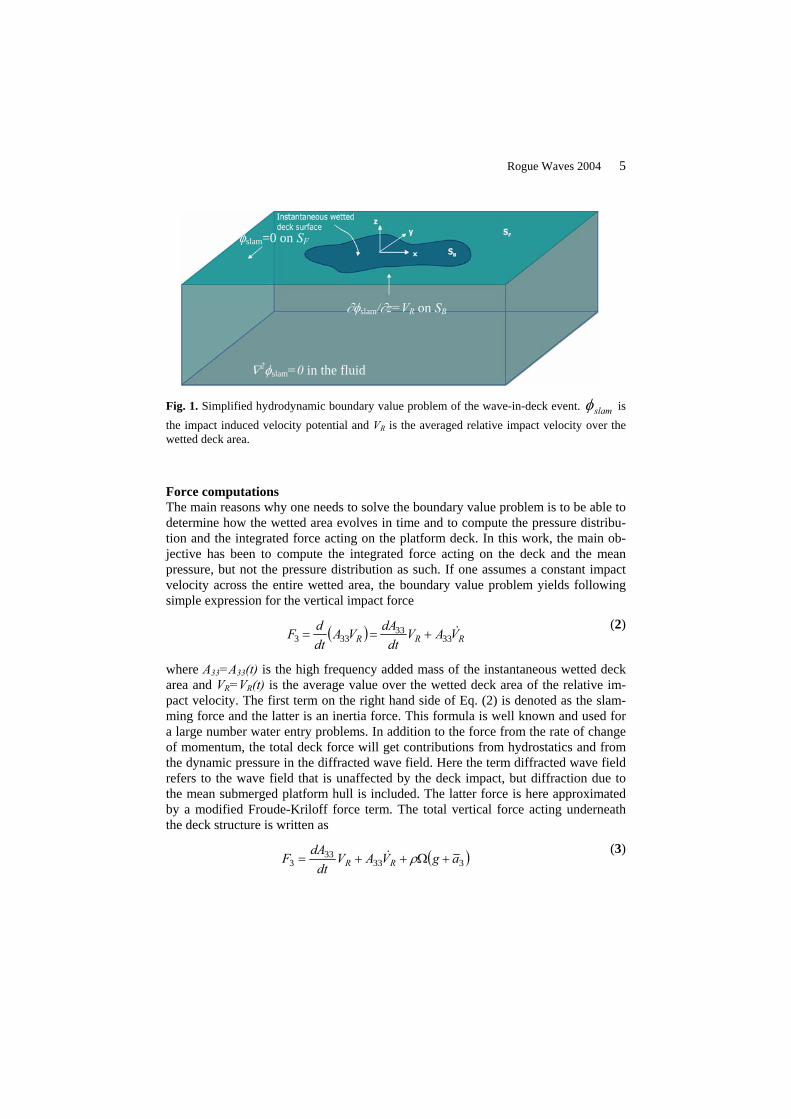
Fig. 1. Simplified hydrodynamic boundary value problem of the wave-in-deck event. slamφ is the impact induced velocity potential and VR is the averaged relative impact velocity over the wetted deck area.
Force computations The main reasons why one needs to solve the boundary value problem is to be able to determine how the wetted area evolves in time and to compute the pressure distribu-tion and the integrated force acting on the platform deck. In this work, the main ob-jective has been to compute the integrated force acting on the deck and the mean pressure, but not the pressure distribution as such. If one assumes a constant impact velocity across the entire wetted area, the boundary value problem yields following simple expression for the vertical impact force
( ) RRR VAVdt
dAVAdtdF &
3333
333 +== (2)
where A33=A33(t) is the high frequency added mass of the instantaneous wetted deck area and VR=VR(t) is the average value over the wetted deck area of the relative im-pact velocity. The first term on the right hand side of Eq. (2) is denoted as the slam-ming force and the latter is an inertia force. This formula is well known and used for a large number water entry problems. In addition to the force from the rate of change of momentum, the total deck force will get contributions from hydrostatics and from the dynamic pressure in the diffracted wave field. Here the term diffracted wave field refers to the wave field that is unaffected by the deck impact, but diffraction due to the mean submerged platform hull is included. The latter force is here approximated by a modified Froude-Kriloff force term. The total vertical force acting underneath the deck structure is written as
( )33333
3 agVAVdt
dAF RR +Ω++= ρ&
(3)
φslam=0 on SF
∂φslam/∂z=VR on SB
∇2φslam=0 in the fluid

Rogue Waves 2004 6
where ρ is the water density and Ω= Ω (t) is the instantaneous volume of fluid in the diffracted wave that is above the lower deck. For simplicity, 3a is taken as the aver-age vertical fluid acceleration in the diffracted wave at the instantaneous wetted area. Thus, RVa &=3 for a stationary platform. The same type for formulation was used to Baarholm and Faltinsen [15] for two-dimensional wave-in-deck impact. The slam-ming term is set equal to zero during water exit. This treatment is based on the con-sideration of vertical momentum transfer only upon water entry and not during condi-tions associated with water exit. Such treatment is used in ship slamming analysis (see [11]) and is carried over to the present case. The same approach is used by e.g. [5] and [8]. Equation (3) shows that the vertical force due wave impact underneath a platform deck is governed by the kinematics in the wave crest in combination with the plat-form motions and the evolution of the high frequency limit of the added mass of the wetted deck area. An exact solution for the evolution of the wetted area cannot be found without solving the boundary value problem. Here, however, assume that the instantaneous wetted deck area can be approximated by a von Karman approach. This means that the wetted area is found from the intersection between the diffracted wave field, excluding diffraction effects from the impact potential, and the deck. When the wetted area is known, one can compute the added mass of this. Kaplan used a for-mula similar to (3) to compute the vertical wave-in-deck force on jacket platforms. In addition to the terms in the above expression, Kaplan also included a drag term in the force expression. He limited his analyses to long-crested head or beam sea waves relative to the rectangular deck. This means that the wetted deck area is rectangular at all times, and that he could solve the problem by a two-dimensional analysis. More-over, he applied a von Karman type approach when evaluating the wetted deck area, i.e. the wetted area was found as the geometrical intersection between the deck and the undisturbed free surface. Since the wetted area was rectangular, the added mass could be found by analytical expressions. Consequently, the impact loads could be assessed without solving the boundary value problem as such. The idea here is to generalize Kaplan’s approach so that it can be applied for three-dimensional impact problems for which diffraction effects from the presence of a large-volume structure are accounted for. For such a case the wetted area due to im-pact may have a more general shape, and analytical expressions for the added mass cannot be found. In principle, the added mass must be evaluated numerically for each time step. This can be achieved by a three-dimensional panel method. To omit having to solve such a problem, an approximate approach is proposed. Analytical expres-sions for the added mass exist for thin rectangular plates and thin elliptical disks. The general idea is to approximate the wet area by one of these basic geometries. This enables us to estimate the added mass with explicit analytical expressions. The feasi-bility of using the added mass of elliptical disks or rectangular plates has been stud-ied. An extract of the study is presented in [16]. The general conclusion was that one can get good estimates of the added mass of arbitrarily shaped thin plates by applying the added mass of a representative elliptical or rectangular plate. When fitting the

Rogue Waves 2004 7
general shaped plate to one of the basic geometries it is important to keep the area of the model plate the same as the real wetted area and to use a representative aspect ratio.
Relative impact velocity and acceleration The vertical fluid velocity and acceleration at the deck level are found to second or-der. In the following the velocity potential φwave is split into a first and second order part so that
( ) ( ) ( )321awave O ζφφφ ++= (4)
where ζa is the amplitude of the first order incident wave. φ(1)(x,y,z,t) and φ(2)(x,y,z,t) are the first and second order wave potentials (incident wave + diffracted wave due to the mean submerged part of the hull). By use of Taylor expansion to ( )2
aO ζ , the rela-tive vertical fluid velocity at the deck can be expressed as
deckdeck zzzw ηφηφφ
&−∂∂
+∂
∂+
∂∂
= 2
)1(2)2()1(
(5)
where the quantities z∂∂ )1(φ , z∂∂ )2(φ and 2)1(2 z∂∂ φ are to be evaluated on z=0.
),,( tyxdeckdeck ηη && = is the vertical velocity of the deck. This quantity vanishes for a stationary platform. VR is taken as the average value of w over the wetted area. Simi-larly, RV& is taken as the average value of w& .
Validity of second order diffraction analysis The free-surface wave elevation and kinematics is disturbed due to the presence of the large-volume structure. The structure in case study below consists of three col-umns and a large caisson. This is an important factor in the wave-in-deck problem, leading to the input condition of the impact model described above. The prediction of elevation around vertical columns in steep waves, by use of linear as well as second-order numerical diffraction models, has been validated in [6,7]. From these works, it is found that while the use of linear theory can lead to significant under-estimation, second-order models can in many cases work fairly well even in steep waves. The largest discrepancies are observed for high column-to-wavelength ratios (kζa > 0.4), particularly due to over-predictions of the sum-frequency terms. For low kζa-values, the agreement is better, while there are still some discrepancies due to effects beyond second order. Generally speaking, this can lead to under-prediction in the vicinity of the columns, and some over-prediction further away.
3 Present Implementation
The theory described above is implemented into a computer program. Below, the main steps in the numerical simulation are described in brief. A priori diffraction

Rogue Waves 2004 8
analysis of the submerged part of the hull must be performed. In the present work second order frequency-domain diffraction analysis is performed by applying WA-MIT (see [12]). Linear and quadratic transfer functions of wave kinematics and free surface elevation at a large number of field points below the deck is evaluated. The computed hydrodynamics are used as input to the simulation program. The field points are distributed in two horizontal layers. One layer is located at the mean free surface with the second layer just below. Two layers are needed to evaluate the z-derivative of the computed hydrodynamic quantities. These are needed to extrapolate the wave kinematics above the mean free surface.
In the case of regular waves, the diffracted wave field underneath the deck structure is evaluated for each time step by use of
( ) ( )( ) )2(2)2(2)1( ~2exp~exp~Re),,( −+ ++= ηζωηζωηζζ aaa titityx (6)
where ω is the oscillation frequency of the incident wave. The η~ ’s are complex lin-ear and quadratic transfer function values from WAMIT, all dependent upon spatial position although this is not explicitly stated in the expression. Note that the term
( )−2~η is real while the other terms are complex. The superscripts (2+) and (2-) denote
second order sum- and difference frequency contributions, respectively. ( )1~η gives the
linear contribution. When knowing the diffracted wave field, approximate values of the instantaneous wetted area, A33 and wave kinematics can be evaluated. The impact event is stepped forward in time until the wave has completely detached from the deck. Consequently, the vertical force on the deck can be evaluated from Eq. (3).
4 Validation case: Wave-in-deck loads on the Statfjord A GBS
A model test program on the Statfjord A GBS was undertaken in the Ocean Basin at Marintek to assess wave-in-deck loads (see [1]). The main objective was to determine hydrodynamic loads from extreme waves on the platform deck at various water depths, to study the effect of estimated future seabed subsidence. Two depths were tested: 150.1m (as-is today) and 151.6m, measured from still water level to the sea bottom. These water depths leave 23.2m and 21.7m air-gap, respectively; from the cellar deck (see Fig. 2). The GBS has 3 columns. The deck on the Statfjord A platform is 83.60m long and 54.24m wide. In addition it has two extensions protruding from each of the decks long side. The dimensions of these are 13.20m by 16.00m. The measurements covered horizontal and vertical wave loads on the deck structure, air gap at critical locations, local slamming loads and measurements of wave amplification due to the large volume structure. Model tests were run with both regular waves and extreme wave packages. Two wave head-ings were tested (see Fig. 2). With the coordinate system used here, the wave head-ings are 240deg and 270deg.

Rogue Waves 2004 9
54.24 m
83.60 m
13.20 m
16.00 m
Wave, 270 deg.Wave, 240 deg.
x
y
(a) Cellar deck outline from above (b) GBS with today’s air-gap
Fig. 2. GBS model with simplified topside (from [1])
Further information about the model tests can be found in [1].
Numerical model
WAMIT was used to perform a priori second order diffraction analysis. The panel model applied in the computations comprised of 5060 panels on the body and 6060 panels on the free surface. A total of 9800 field points were specified for the WAMIT analysis. Note that the field points, which are used when determining the instantane-ous wetted area, cover a rectangular area equal to 83.60m by 54.24m. This means that the extensions on each of the long sides of the deck are not accounted for in the analysis.
Results
The maximum crest elevation obtained by use of the second-order WAMIT model has been validated by comparison to model test measurement. In Fig.3 this is shown for a wave condition H=30m, T=15.5s, 270deg heading. (The actual wave–in-deck load study included higher waves, up to 40m, but they are not included in the eleva-tion study due to the deck interaction effects). Note that the coordinate system is rotated relative to Fig. 2. Results from linear theory, second-order theory and meas-urements at various locations are shown. Notice that in the present case, the scattering parameter ka is as low as approximately 0.1, which means that we are in the range where the second-order theory is found to work reasonably well [7]. Further results from this and other case studies analysis are presented in [7, 17].
Not included in analysis

Rogue Waves 2004 10
Fig. 3. Comparison of maximum crest elevation in wave field under the platform
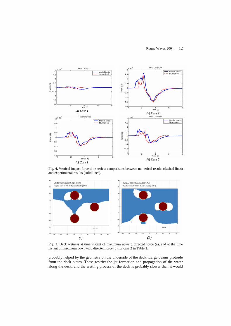
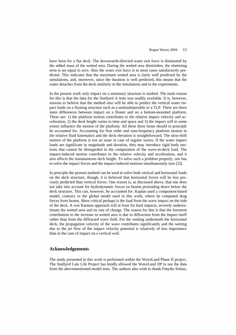
The numerical load simulation program has been used to reproduce the wave-in-deck events. The analysis is limited to the regular wave tests. In this paper, results are reported for the tests with heading 270deg and with a deck height corresponding to a seabed subsidence of 1.5m. This adds up to altogether 7 test cases. Results from oblique sea computations are presented in [16]. Table 1 presents the main results. Both the maximum water entry force and the maximum magnitude of the negative water exit force from the experiments and the numerical simulations are listed in the table. However, not only the maximum and minimum force were found, the entire time history of the impact force has been simulated for each of the 7 test cases. Ex-ample plots of the simulated time series compared to the measured forces records are given in Fig. 4. Plots showing the wetness of the deck at the time instants of maxi-mum and minimum force for case 2 are given in Fig. 5.

Rogue Waves 2004 11
Table 1. Results from numerical computation of wave-in-deck impact due to regular incident waves. H and T are wave height and period, respectively. Maximum upward directed force (Fmax) and maximum downward directed force (Fmax) are reported. Corresponding experimental results are included.
Measurements Numerical results Case No.
H (m)
T (s)
Fmax (MN)
Fmin (MN)
Fmax (MN)
Fmin
(MN) 1 2 3 4 5 6 7
34.0 40.0 37.0 34.0 37.0 34.0 33.0
17.0 17.0 15.5 15.5
16.25 16.25 14.0
7.8 166.4 51.0 15.2 70.8 7.5 45.3
-23.9 -131.9 -91.2 -23.7 -78.8 -18.7 -30.1
7.4 140.2 53.4 16.7 67.3 9.3 8.3
-12.3 -153.6 -95.3 -23.0 -84.2 -17.0 -23.1
5 Discussion and Conclusions
The diffracted elevation of the second-order model compares reasonably well to measurements in this case. Furthermore, it can be concluded that use of linear eleva-tion theory may lead to significant under-prediction of both the occurrence and sever-ity of wave-in-deck events. Linear waves would not give impact for any of the 7 cases analyzed.
In general, good agreement is also obtained between the numerical method and the experiments for the loads of hardest water impacts. Both the magnitude of the water entry force and the water exit force as well as the duration of the wave-in-deck event is satisfactory predicted. For the softer impacts, when the wave is barely reaching the deck structure, the relative difference between the measured force and the computed force is greater. This is as expected and in accordance with the experience presented in [8]. When the wave is just reaching the deck, great accuracy in both the wave ele-vation and the fluid particle kinematics are required to get good correspondence be-tween measurements and computations. Case no. 1 in Table 1 is an example of such a soft impact event. The resulting force for such mild impacts is however small, and the absolute errors in the computed force is therefore also moderate. On the other hand, slight inaccuracies in the generated waves or in the numerical solution of the free surface elevation and fluid particle kinematics will give smaller relative errors for severe impacts. The absolute errors may be significant but the computed results al-ways indicate the magnitude of the impact force.
The experience from [8] would indicate that a von Karman method should underesti-mate the magnitude of the upwards-directed slamming force. This is also the case here, but perhaps to a lesser extent than expected. The reason why a simple von Kar-man approach would under-estimate the slamming force is that diffraction due to the deck is omitted and dA33/dt is thus underestimated. Karman approach would under-estimate the slamming force is that diffraction due to the deck is omitted and dA33/dt is thus underestimated. The von Karman approach performs well here, but it is
Rogue Waves 2004 12
(a) Case 1
(b) Case 2
(c) Case 3
(d) Case 5
Fig. 4. Vertical impact force time series: comparisons between numerical results (dashed lines) and experimental results (solid lines).
(a)
(b)
Fig. 5. Deck wetness at time instant of maximum upward directed force (a), and at the time instant of maximum downward directed force (b) for case 2 in Table 1.
probably helped by the geometry on the underside of the deck. Large beams protrude from the deck plates. These restrict the jet formation and propagation of the water along the deck, and the wetting process of the deck is probably slower than it would
Rogue Waves 2004 13
have been for a flat deck. The downwards-directed water exit force is dominated by the added mass of the wetted area. During the wetted area diminishes, the slamming term is set equal to zero. Also the water exit force is in most cases satisfactorily pre-dicted. This indicates that the maximum wetted area is fairly well predicted by the simulations, and, moreover, since the duration is well predicted, this means that the water detaches from the deck similarly in the simulations and in the experiments. In the present work only impact on a stationary structure is studied. The main reason for this is that the data for the Statfjord A tests was readily available. It is, however, reasons to believe that the method also will be able to predict the vertical water im-pact loads on a floating structure such as a semisubmersible or a TLP. There are three main differences between impact on a floater and on a bottom-mounted platform. These are: 1) the platform motion contributes to the relative impact velocity and ac-celeration, 2) the deck height varies in time and space and 3) the impact will to some extent influence the motion of the platform. All these three items should in principle be accounted for. Accounting for first order and sum-frequency platform motion in the relative fluid kinematics and the deck elevation is straightforward. The slow-drift motion of the platform is not an issue in case of regular waves. If the water impact loads are significant in magnitude and duration, they may introduce rigid body mo-tions that cannot be disregarded in the computation of the wave-in-deck load. The impact-induced motion contributes to the relative velocity and acceleration, and it also affects the instantaneous deck height. To solve such a problem properly, one has to solve the impact forces and the impact-induced motions simultaneously (see [2]). In principle the present method can be used to solve both vertical and horizontal loads on the deck structure, though, it is believed that horizontal forces will be less pre-cisely predicted than vertical forces. One reason is, as discussed above, that one does not take into account for hydrodynamic forces on beams protruding down below the deck structure. This can, however, be accounted for. Kaplan used a component-based model, contrary to the global model used in this work, where he computed drag forces from beams. More critical perhaps is the load from the wave impact on the side of the deck. A von Karman approach will at least for hard impacts, severely underes-timate the wetted area and its rate of change. The reason for this is that the foremost contribution to the increase in wetted area is due to diffraction from the impact itself rather than from the diffracted wave field. For the wetting underneath the horizontal deck, the propagation velocity of the wave contributes significantly and the wetting due to the jet flow of the impact velocity potential is relatively of less importance than in the case of impact on a vertical wall.
Acknowledgements
The study presented in this work is performed within the WaveLand Phase II project. The Statfjord Late Life Project has kindly allowed the WaveLand JIP to use the data from the abovementioned model tests. The authors also wish to thank Frøydis Solaas,

Rogue Waves 2004 14
Trygve Kristiansen and Vibeke Moe for valuable contributions to the numerical mod-eling and data analysis.
References
1. Stansberg C.T., Baarholm R., Fokk T., Gudmestad O.T. and Haver S. : Wave amplification and possible wave impact on gravity based structure in 10-4 probability extreme crest heights, OMAE 2004-51506. Proc. 23rd OMAE Conf., Vancouver, Canada (2004)
2. Baarholm, R, O.M. Faltinsen and K. Herfjord : Water impact on decks of floating plat-forms. Proc. 8th Int. Symp. on Practical Design of Ships and other Floating Structures (PRADS2001). Elsevier, Oxford. (2001).
3. Baarholm, R and O. Faltinsen: Wave impact underneath horizontal decks. J. Mar Sci Tech-nol, 9, (2004) 1-13.
4. Health & Safety Executive: Review of wave in deck load assessment procedure. Offshore Technology Report – OTO 97 073, (1998).
5. Kaplan P.: Wave impact on offshore structures: re-examination and new interpretations. Proc. 24th Offshore Technology Conference, Houston, USA. (1992)
6. Kristiansen T, Baarholm R. and Stansberg C.T.: Validation of Second-Order Analysis in Predicting Diffracted Wave Elevation around a Vertical Circular Cylinder. Proc. 14th ISOPE, Toulon, France. (2004).
7. Stansberg C.T. and Kristiansen T.: Non-linear scattering of steep waves around vertical columns. Submitted for publication (2005).
8. Baarholm R.: Theoretical and experimental studies of wave impact underneath decks of offshore platforms. PhD Thesis, Norwegian University of Science and Technology (NTNU), Trondheim, Norway. (2001)
9. Von Karman T.: The impact on seaplane floats during landing. In National Advisory Com-mittee for Aeronautics, NACA, (1929) 309-313.
10. Wagner H.: Über Stoß- und Gleitvorgänge an der Oberfläche von Flüssigkeiten, ZAMM, 12, (1932) 192-126
11. Kaplan P.: Analysis and Prediction of Flat Bottom Slamming Impact of Advanced Marine Vehicles in Waves. Int. Shipbuilding Progress, March (1987).
12. Lee C.-H.: WAMIT Theory Manual, Report No. 95-2, Dept. of Ocean Engineering, Massa-chusetts Institute of Technology (MIT), Cambridge, Mass., USA. (1995)
13. Zhao R. and Faltinsen O.M.: Slamming Loads on High-Speed Vessels. In W. D. C. Na-tional Academy Press (Ed.), Proc. of the 19th ONR Conference, Seoul, South Korea (1992).
14. Faltinsen O.M. and Zhao R.: Water entry of ship sections and axisymmetric bodies. Advi-sory Group for Aerospace Research and Development, AGARD REPORT R-827 (1998).
15. Baarholm R and Faltinsen O.M.: Experimental and theoretical studies of wave impact on an idealized platform deck. Proc. of the 4th Int. Conf. on Hydrodynamics (ICHD 2000), Yokohama, Japan. (2000)
16. Baarholm R.: A Simple Numerical Method for Evaluation of Water Impact Loads on Decks of Large-Volume Offshore Platforms. In Proc. OMAE 2005, Paper no. OMAE2005-67097, Halkidiki, Greece (2005).
17. Stansberg, C.T., Baarholm, R., Kristiansen, T., Hansen, E.W.M and Rørtveit, G.: Extreme Wave Amplification and Impact Loads on Offshore Structures. In Proc. OTC 2005, Paper No. 17487, Houston, TX, USA (2005).

Violent water wave impacts on a wall
Howell Peregrine, Henrik Bredmose, Mathematics, University of Bristol, U.K. [email protected], [email protected],
Geoffrey Bullock, Charlotte Obhrai, Civil & Structural Engineering, University of Plymouth, U.K. [email protected], [email protected]
Gerald Müller∗, Guido Wolters Civil Engineering , Queen’s University, Belfast, U.K. [email protected], [email protected]
Violent impact of an extreme wave onto a structure can be the criterion that determines a number of design parameters. Within the BWIMCOST (Breaking Wave IMpacts on COastal STructures) project such impacts have been measured in the field and the laboratory for waves breaking onto a sea wall or breakwater, see Bullock et al. (2003). The time and space scales of impact are sufficiently small that the hydrodynamics of impact is unlikely to differ for waves in deep water which hit fixed or floating structures. In practical situations when pressures exceed a few atmospheres, it is appreciated that compressibility of air becomes important. This is particularly so for air that is entrained into or trapped by water, so special efforts have been made to measure the air-fraction in the water. Peregrine (2003) is a recent review: work subsequent to that review is reported here. The overturning jet of the breaker may trap a ‘pocket’ of air, and/or the water may have already entrained a multitude of air bubbles. Both types of air distribution influence the effect of wave impact, due to their greater compressibility compared with pure water. The compressibility, evident in the very low velocity of sound in the air-water mixtures that occur as and after waves break, is a primary concern when small-scale laboratory data is being used to estimate large-scale prototype impacts, since the usual Froude scaling is unlikely to be correct. The three main strands of data are from prototype:
1) the Admiralty breakwater, Alderney, which is exposed to waves from the Atlantic Ocean. 2) 1:4 scale: in the big wave channel (Grosser Wellenkanal, GWK) Hanover. 3) 1:25 scale: laboratory experiments in Plymouth with both fresh and sea water.
Figure 1. Wave impact on a wall sloping at 27º to the vertical. Spray caused by air escaping from a trapped air pocket at high pressure can be seen. The exposure time is 1/125 second, and the width of the flume (GWK) is 5 metres.
Few examples of violent impacts have been obtained from Alderney, the most severe impact occurred on an otherwise quiet day and may be described as a rogue wave. On the other hand the GWK measurements have yielded exceptionally violent impacts with pressures up to 3 MPa. These impacts vary in character, some details will be presented. The theoretical studies include
a) careful analysis of the data for waves approaching the breakwater, and for the impacts.
b) development of simple mathematical models.
c) development and study of detailed numerical models.
Here attention is focussed on the detailed modelling.
∗ at Southampton University from January 2005.

Waves approaching the wall are approximated with irrotational flow for which a boundary-integral computation is used Tanaka et al. (1987). This computation stops when the wave hits the wall or the flow becomes too violent, rough, or a jet extends too far.
Figure 2 Wave profiles from a boundary-integral computation of a wave propagating over a berm towards a wall.
The compressible model. is the simplest possible, essentially the two-dimensional unsteady Euler equations for an air-water mixture with variable air volume fraction. It assumes adiabatic compression of the air and no relative movement between the phases. There are numerical problems with such a model when shock waves pass from light medium to a denser one, but, so far, they do not seem to be of importance in the first few wave impact examples that have been run at the time of writing. The initial conditions for the compressible flow computations are taken for a region near the wall from the boundary-integral computation: for example, from a profile which is intermediate between the last two in figure 2. The computations provide a complete time history for the flow field and pressure on and near the structure. The analysis of these computations is in progress. Support from EPSRC; E.U. Access to Research Infrastructures action; the co-operation of Joachim Grüne (GWK) and the breakwater maintenance staff on Alderney are gratefully recognised. Bullock, G., Obhrai, C., Müller, G., Wolters, G., Peregrine, H. & Bredmose, H., (2003) Field and
laboratory measurements of wave impacts. Proc. Int. Conf. Coastal Structures 2003. ASCE, to appear
Peregrine, D.H. 2003 Water wave impact on walls, Ann. Rev. Fluid Mech. 35, pp.23-43. Tanaka, M., Dold, J.W., Lewy, M. & Peregrine. D.H. (1987) Instability and breaking of a solitary
wave, Jour. Fluid Mech. 185, pp.235-248.
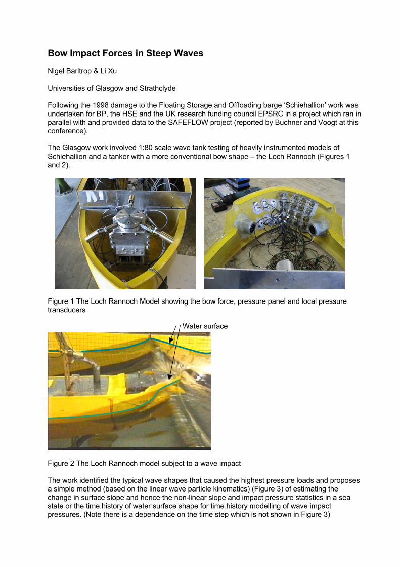
Bow Impact Forces in Steep Waves Nigel Barltrop & Li Xu Universities of Glasgow and Strathclyde Following the 1998 damage to the Floating Storage and Offloading barge ‘Schiehallion’ work was undertaken for BP, the HSE and the UK research funding council EPSRC in a project which ran in parallel with and provided data to the SAFEFLOW project (reported by Buchner and Voogt at this conference). The Glasgow work involved 1:80 scale wave tank testing of heavily instrumented models of Schiehallion and a tanker with a more conventional bow shape – the Loch Rannoch (Figures 1 and 2). Figure 1 The Loch Rannoch Model showing the bow force, pressure panel and local pressure transducers
Figure 2 The Loch Rannoch model subject to a wave impact The work identified the typical wave shapes that caused the highest pressure loads and proposes a simple method (based on the linear wave particle kinematics) (Figure 3) of estimating the change in surface slope and hence the non-linear slope and impact pressure statistics in a sea state or the time history of water surface shape for time history modelling of wave impact pressures. (Note there is a dependence on the time step which is not shown in Figure 3)
Water surface

0.25 0.28 0.32 0.35 0.38 0.42 0.450
1
2
3
4
5
Acceleration/g
Mea
sure
d Sl
ope/
Line
ar C
alcu
late
d Sl
ope
Figure 3 Increase in wave front steepness relative to a linear random model of the water surface The bow forces may be calculated using a rate of change of added mass calculation in conjunction with the wave shape data (Figure 4). Alternatively pressures may be calculated using a slam force equation with additional terms to account for the size of the panel (non dimensionalized by bow width and wave height) for which the pressure is required.
DAFVZGWFSCEg
P s2)()()(1
=
Where P is the estimated pressure in m head water C is a constant E(S) is dependent on sea state steepness (S) F(W) is dependent on panel width (W) G(Z) is dependent on panel height (Z) Vs is the slam velocity ( velocityparticlexcelerity ) DAF is the dynamic amplification factor The results were input to a reliability analysis (performed with other SAFEFLOW partners) to estimate combinations of sea state return periods and safety factors that should be used for structural design. As a result of the larger uncertainties in impact loads than in ordinary wave loading, slightly larger safety factors are recommended.
Figure 4 Visualisation of mathematical model used in conjunction with a rate of change of added mass calculation of slam force
XDN YDN, ZDN,( ) XDN YDN−, ZDN,( ), XP YP, ZPS,( ), XF1 20+ YF1, ZF1,( ), XF1 55+ YF1, ZF1,( ), XF1 90+ YF1, ZF1,( ),
Water surface For slam calculation replaced by a parabolic surface defined by the intersection of the true surface and the three planes
Hull strips For finding width and hence added mass at the water surface intersection of each strip
Planes normal to hull For relative water surface elevation calculation

ROGUE WAVES 2004, SeaTechWeek 2004, Brest, France
Enhanced wave effects on the weather sideof reflective structures
B. Molin, F. Remy, O. Kimmoun, E. Jamois
Ecole generaliste d’ingenieurs de Marseille, 13 451 Marseille cedex 20
Strong wave effects are often observed on the weather side of marine or coastal structures.An example is wave runup, experienced by ships in beam waves and some offshore structures.These runup effects are sometimes far above design values, suggesting some ”anomaly” of theincoming waves.
It is advocated that the incoming wave system can actually be modified through its non-linear interaction with the reflected wave system from the structure. This statement is basedon extensive model tests, performed at BGO-First in la Seyne sur mer, and on theoretical andnumerical analyses.
The experimental model consisted in a vertical plate, projected from one of the side-walls ofthe basin. It was submitted to regular waves of varying wavelengths and steepnesses, in deepwater conditions (kh > 3). At wavelengths comparable with the width of the plate, strongrunups are observed at the plate-wall intersection, increasing with the wave steepness. Theserunups take many wave cycles to develop, with no steady-state being reached in some cases.Free surface elevations as high as 5 times the amplitude of the incoming waves have been mea-sured in some cases, far above calculated values with numerical models based on linearizedpotential flow theory.
A simple theoretical model is proposed, based on tertiary (third-order) wave interaction, asfirst given by Longuet-Higgins & Phillips (1962). A parabolic equation is derived, that describesthe space evolution of the amplitude of the incoming waves through their tertiary interactionwith the reflected waves (locally idealized as plane waves). A steady-state solution is obtainedthrough iterations, where the incoming and reflected wave systems are successively updated.Details can be found in Molin et al. (2005). The figure shows the incoming wave system onthe weather side of the plate, obtained at the end of this process, for a steepness H/L of 4 %and a wavelength equal to the length of the plate (1.2 m): the incoming wave amplitude hasnearly doubled as it reaches the plate (in x = 0).
The numerical model is based on the enhanced Boussinesq equations as first proposed byAgnon et al. (1999) and Madsen et al., and further developed by Fuhrman & Bingham (2004).
It is noteworthy that these nonlinear (tertiary) interactions between the incoming and re-flected waves have some similarity with shoaling: the incoming waves are ”slowed down”,the wavelength decreases, the crest-lines bend and the wave energy gets focused toward theplate-wall intersection. As a matter of fact our parabolic equation resembles the parabolic

-6
-5
-4
-3
-2
-1
0
x (m)
1
2
3
4
y (m)
Figure 1: Three-dimensional view of the incoming waves by the plate.
approximation of the mild slope equation.
Numerical investigations have shown that the effective interaction area, between the incom-ing and reflected waves, can extend many wavelengths upwave. Contrary to intuition, theinteraction area increases when the wavelength decreases, meaning that the incoming waveamplitude is being affected further and further from the plate.
Similar effects are expected to occur for other reflective bodies, such as multi-legged platformsor coastal structures.
References
Agnon Y., Madsen P.A. & Schaffer H.A. 1999 A new approach to high-order Boussinesqmodels, J. Fluid Mech., 399, 319-333.Fuhrman D.R. & Bingham H.B. 2004 Numerical solutions of fully non-linear and highlydispersive Boussinesq equations in two horizontal dimensions, Int. J. Numer. Meth. Fluids,44, 231-255.Longuet-Higgins M.S. & Phillips O.M. 1962 Phase velocity effects in tertiary wave in-teractions, J. Fluid Mechanics, 12, 333-336.Madsen P.A., Bingham H.B. & Liu H. 2002 A new Boussinesq method for fully nonlinearwaves from shallow to deep water, J. Fluid Mech., 462, 1-30.Molin B., Remy F., Kimmoun O. & Jamois E. 2005 The role of tertiary wave interactionsin wave–body problems, J. Fluid Mech., 528, 323–354.

ROGUE WAVES 2004
ABSTRACT
On the shape of large waves in the central and southern North Sea
Anne Karin Magnusson [email protected]
Norwegian Meteorological Institute Allégaten 70, 5007, Bergen, Norway
Alessandro Toffoli [email protected] Hydraulics Laboratory, K. U. Leuven
Kasteelpark Arenberg 40, B-3001, Heverlee, Belgium
Jaak Monbaliu [email protected] Hydraulics Laboratory, K. U. Leuven
Kasteelpark Arenberg 40, B-3001, Heverlee, Belgium
Elzbieta Bitner-Gregersen [email protected]
Det Norske Veritas AS N-1322 Høvik, Norway
Within the past two decades, a large amount of super carriers have been lost at sea. In some cases the losses are likely to be related to severe weather conditions. "Freak" or "rogue" waves are sometimes mentioned as probable cause. These terms are used to point at individual waves of exceptional wave height or abnormal shape. And it is, in particular, their shape that is of great importance for the design and operation of ships and offshore structures, as it can lead to significant impact damages. The present paper provides results of deterministic analysis concerning wave front steepness and horizontal asymmetry that was carried out on data collected at the Ekofisk field, central North Sea (operated by ConocoPhillips) and at several locations off the Belgian coast during a period of 6 months. The Belgian data are collected from different locations and water depth off the Belgian coast, using non-directional buoys, operated by the Ministry of the Flemish Community. Wave records have been recorded continuously at the sample frequency of 2 Hz since January 2003. The Ekofisk data analysed here consist of one-dimensional time series of wave profile, also collected at a sampling frequency of 2 Hz. Data from a Waverider buoy and two down looking lasers are used. Time domain parameters are calculated using a zero down-crossing analysis over a time period of 20 minutes. Concern is taken on the quality control of the data, since shape parameters are quite dependent on how small variations on larger waves are handled. Shape parameters during extreme conditions are compared to average values, and variations from finite to infinite water depth are demonstrated. Recent work (i.e. Olagnon and Magnusson, 2004) indicate that extremes occur due to changes on smaller time scales than 20 minutes, so variations of shape parameters over smaller time scales are also analysed here. Results on i.e. horizontal asymmetry are compared to literature (Olagnon and Krogstad, 1998, Myrhaug and Kjeldsen, 1986, Stansell et al., 2003). Myrhaug D., Kjeldsen S.P, 1986: “Steepness and symmetry of extreme waves and the highest wave in deep water”. Ocean Eng 1986; 13(6), pp549-86
….

Olagnon, M., and H.E.Krogstad, 1998: “Observed short- and long-term distributions of wave steepness”. Proc. Int. Offshore and Polar Engineering Conf., Vol. 3, Montreal, pp. 63-70. Olagnon, M., and A.K.Magnusson, 2004: “Sensitivity Study of Sea State Parameters in Correlation to Extreme Wave Occurrences”. Proc. of ISOPE’2004, Toulon, May 23.-27. Stansell P., Wolfram J., Zachary S., 2003: “Horizontal asymmetry and steepness distribution for wind-driven ocean waves from severe storms”. Applied Ocean Research 2003; 25, pp137-55

1
Exploring Rogue Waves from Observations in South Indian Ocean
Paul C. Liu1, Keith R. MacHuchon2 , and Chin H. Wu3
1 NOAA Great Lakes Environmental Research Laboratory Ann Arbor, Michigan 48105, U.S.A.
(email: [email protected]) 2 Liebenberg & Stander International (Pty) Ltd
Cape Town, 8000 South Africa (email: [email protected])
3 University of Wisconsin-Masison, Madison, Wisconsin 53706, U.S.A.
(email: [email protected] )
Abstract. Amidst all the enticing advancements on rogue waves in re-cent years, the conspicuous scarcity of actual, in situ, rogue wave meas-urements still represents an inevitable hindrance shadowing over the horizon of rogue wave studies. In this paper we wish to present an exploratory observational study of rogue waves based on wave meas-urement made in South Indian Ocean. As there have been significant theoretical advancements in numerical simulation of rogue waves, the need for actual field observations of rogue waves should certainly be commensurably supplemented. We hope our efforts in this study can be ventured toward further understanding of rogue waves in reality.
1 Introduction
Amidst all the enticing advancements on rogue waves in recent years, the conspicu-ous scarcity of actual, in situ, rogue wave measurements still represents an inevitable hindrance shadowing over the horizon of rogue wave studies. From the meager ob-servational rogue wave studies based on available wave measurements, on the other hand, the results usually provide objective outcomes that tend to refute rather than confirm some of the familiar conceptualizations of rogue waves. For instance, rogue waves have always been considered to be rare occurrences, but a radar satellite study (e.g. http://195.173.17.24/news/pr2003/2.php) carried out by the German Aerospace Centre recently found 10 monster waves around the world, ranging from 26 m to 30 m in height. They concluded that “it looks as if freak waves occur in the deep ocean far more frequently than the traditional linear model would predict.” Another recent study by Liu and Pinho (2004) based on wave measurements made from Campos
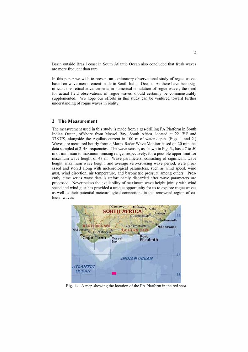
2
Basin outside Brazil coast in South Atlantic Ocean also concluded that freak waves are more frequent than rare.
In this paper we wish to present an exploratory observational study of rogue waves based on wave measurement made in South Indian Ocean. As there have been sig-nificant theoretical advancements in numerical simulation of rogue waves, the need for actual field observations of rogue waves should certainly be commensurably supplemented. We hope our efforts in this study can be ventured toward further understanding of rogue waves in reality.
2 The Measurement The measurement used in this study is made from a gas-drilling FA Platform in South Indian Ocean, offshore from Mossel Bay, South Africa, located at 22.17ºE and 37.97ºS, alongside the Agulhas current in 100 m of water depth. (Figs. 1 and 2.) Waves are measured hourly from a Marex Radar Wave Monitor based on 20 minutes data sampled at 2 Hz frequencies. The wave sensor, as shown in Fig. 3., has a 7 to 50 m of minimum to maximum sensing range, respectively, for a possible upper limit for maximum wave height of 43 m. Wave parameters, consisting of significant wave height, maximum wave height, and average zero-crossing wave period, were proc-essed and stored along with meteorological parameters, such as wind speed, wind gust, wind direction, air temperature, and barometric pressure among others. Pres-ently, time series wave data is unfortunately discarded after wave parameters are processed. Nevertheless the availability of maximum wave height jointly with wind speed and wind gust has provided a unique opportunity for us to explore rogue waves as well as their potential meteorological connections in this renowned region of co-lossal waves.
Fig. 1. A map showing the location of the FA Platform in the red spot.

3
Fig. 2. A snapshot of the FA Platform.
Fig. 3. Schematic illustration of the platform wave measurement.

4
Fig. 4. Correlation plot of Hmax vs, Hs.
3 Data and Analysis
From an examination of the most recent 6 years data that covered the turn of the mil-lennium, 1998 – 2003, we have found some interesting results, which may or may not be immediately intuitive. Based on the customary criterion of defining rogue waves as Hmax/Hsig > 2, there are 1563 potential rogue wave cases contained in a total record of 50359 hours over the 6 years. A general occurrence rate of 3.1 percent, which is less than, but reasonably close to, the 3.7 percent Liu and Pinho (2004) found from South Atlantic Ocean. These presumably rogue wave cases we examined generally conform to the expectable configurations as shown in Fig. 4 with Hmax/Hsig lying mostly between 2 and 3. However our primary interest have unwittingly engrossed by a number of isolated cases occurred during 1999, 2000, and 2002 where the data appeared to be entirely out of line with the bulk of general conglomeration of the data. These cases show that Hmax hiked up to between 23.2 and 71.4 m and with Hmax/Hsig accordingly varying between 4.5 and 21.3. Are they just simple outliers? Our initial inclination tends to respond affirmatively to the above question. It is usually non-disputive to implicate that the recording can somehow be temporarily in malfunction, so the outliers can be summarily discarded. However, after further de-liberation, and considering the fact that the wave recorder is positioned 20.0 m above mean sea level and most of the outliers are around the wave height sensing limit, we now believe that some of the anomalies may very well be real recordings of waves,

5
including taking tides and surface spray into account. In these cases the maximum wave heights could reasonably be expected to be within the sensing range of 43.0 m or more and thus it generally accounts for all the very high Hmax cases shown in Fig. 4 except the one case with Hmax = 71.4 m which is obviously not justifiable. Since we kept an open mind on outliers, we included all the data in for now. Without the bene-fit of time series data the aforementioned inference is certainly not unreasonable, especially given that the recording operated flawlessly both immediately before and after those instances and throughout the years.
Fig. 5. Hourly data plot of maximum wave heights shown as the upper blue curve and significant wave heights as the lower red curve for the Dec. 9-11, 2002 case.
Fig. 6. Same as Fig. 5 for July 24-25, 1999 case.

6
Fig. 7. Same as Fig. 5 for July 26-28, 2002 case.
Fig. 8. Same as Fig. 5 for Nov. 24-25, 2000 case.
As shown in the plots of sample cases presented in Figs. 5 – 8, these cases were in relatively fully-developed seas, and wind fields were generally quite steady in all cases, there is really no discernable physical reason for these anomalies. One plausi-ble reason for these exceptionally high maximum wave height records could be that the wave monitor was momentarily under water during the over passing of these waves and we are not certain if the wave monitor can still accurately sense the water surface under these circumstances. In any event, the actual wave amplitudes would

7
certainly have been far beyond 20 m. In the end we are inclined to postulate that these cases are actually indicative of the presence of the real rogue waves this area is famed for. If this is true, we can only be thankful that their occurrences did not cause any disastrous damage. [ Recall the lost of passenger liner SS Waratah in this area in late July, 1909. See, e.g., http://www.numa.co.za/sswaratah.htm .]
4 Discussion
One of the consequences of the presence of these large rogue waves shown in the previous section is that they led to unprecedented large ratios of Hmax/Hs. What do these large ratios signify? Are they for real or are they outliers? The central concept of the Rayleigh distribution clearly does not overtly preclude large ratios of Hmax/Hs. One of the well-known equations correlates Hmax/Hs with the number of waves needs for it to occur as
[ ] 21s 2NHH /
max /)ln(/ = . So based on Rayleigh distribution, to have ratios of Hmax/Hs to be 3, 4, 5, 6, for in-stance, it simply requires 6.5x10⁷, 7.9x10¹³, 7.9x10²¹, and 1.9x1031 number of waves to occur. As these are extremely large numbers that can translate into millions of years for it to occur. This is rather unrealistic as well impractical. Basically the Rayleigh approach would consider large ratio of Hmax/Hs case extremely rare occur-rences. Conceivably plausible indications can also come from laboratory experiments such as the one conducted by Wu and Yao (2004). While Hmax/Hs was not included in the publication, the ratio of Hmax/Hs was nevertheless available. They varied from 2.947 to 8.731 along with 6 cases of Hmax/Hs in the 3 to 4 range and 4 cases in the 4 to over 5 range. This is very encouraging. In order for us to be able to directly compare the field data with laboratory data. We have to first normalize the available data with the length parameter gT2, where T is the corresponding mean wave period for each avail-able data set. This is effectively converted the process of correlation of Hmax versus Hs to the correlation of corresponding wave steepnesses between the average condi-tions versus the extreme cases. Of course the field data do not have the wave period when the extreme cases occurred. The results are shown in Fig. 9 that presents a rather more coherent appearance than the Hmax versus Hs results. The laboratory results appropriately situated at the extreme boundary of all the data cases at the low end of the steepness scale. But it is also clearly corresponds to the lower boundary of large wave cases, that provides some indication that the large wave cases may not be simply outliers. Further rationales may also come from the local complicated and perplexing physical environment surroundings where the data were measured. As shown in Fig. 10 this

8
area is dynamically dominated by the Agulhas current from the northeast and from the
Fig. 9. Comparing wave measurement from FA platform in stars with laboratory measurements in closed green circles.

9
Fig. 10. Physical environment of South Indian Ocean area where the wave measure-ments were made.
southeast there are composite wavefronts arising from the the deep sea over long fetches. As medium and long period waves with lengths from 200 m to 1500 m re-fracted by the Agulhas plateau, short waves with wave length of 200 m or less pass-ing across the Agulhas bank and meeting the Agulhas retroflection. At the same time short and medium period waves with length in the range of 200 – 500 m further re-fracted by the oncoming strong Agulhas current. Surrounded by such an varied as-sortment of dynamical interactions, it should not be surprised that very large rogue waves can appear from time to time. That’s what makes the exploration invigorating and an envision of these unusual cases as simply outliers would be frivolous.
Fig. 11. Proposing a new classification of rogue waves
5 Concluding Remarks
While Liu and Pinho (2004) did not consider a 3.7 percent occurrence rate of Hmax/Hs > 2 cases to be of rare occurrence, the 15 recorded anomalous cases with much higher ratios for Hmax/Hs which we discovered from among the 50359 hours of measure-

10
ments in 6 years, with an occurrence rate of 0.03 percent, would certainly befit the pertinent nature of rareness by which rogue waves have been customarily known. So would it be possible that there can be different kind of rogue waves? Upon delibera-tion, we are hereby to propose that may be a new classification for rogue waves can be considered. As shown in Fig. 11, for the cases of ratio range of 2 < Hmax/Hs < 4, which embodies most of currently known and available data and analysis, we call them the “typical rogue waves.” For the cases of Hmax/Hs ratios of 4 or higher, we propose to call them the “uncommon rogue waves.” This action will not interfere with the current ongoing rogue wave studies. But this does provide a new realm for the past, present and future seemingly outlier cases to reside. Though these may merely be our speculations, we do feel strongly that the existence of these cases fur-ther emphasizes the crucial need for long-term wave time series measurements for studying rogue waves. Without tangible measurements, no amount of theoretical simulations can truly divulge the reality of the phenomenon so long as we still do not have the slightest notion as to whatever is really happening out there. Acknowledgements
The authors gratefully acknowledge Petro SA, the owners of the Platform, and the CSIR of South Africa, who generously made the information used in this paper avail-able to us.
References
1. Liu and Pinho, 2004, Freak waves - more frequent than rare! Annales Geophysicae, Vol. 22, 1839-1842.
2. Wu, C.H. and Yao, A., 2004 Laboratory measurements of limiting freak waves on cur-
rents, J. Geophysical Research-Oceans, 109, C12, C12002, 1-18.

Development of Operational Guidance Criteria for Small Craft Operating in Dangerous Seas
Bruce Johnson, US Naval Academy, Annapolis,, MD 21402, USA
Tel: +1-410-295-9393; Fax +1-410-293-2219; e-mail: [email protected] Stefan Grochowalski, Ottawa, Canada
The most dangerous seas to small craft operation are those which produce groups of extreme, steep waves (relative to the size of the vessel) and those that involve breaking waves impacting from the beam or astern quartering directions. Rogue waves of twice the significant wave height are certainly dangerous to vessel operation, but groups of steep waves which are large relative to the vessel size are far more likely to be encountered and are equally dangerous. The paper presents additional analysis of the comprehensive model tests of fishing vessel capsizing carried out by the National Research Council of Canada in the 1980s. The analysis is focused on those dangerous elements of ship behavior in large, steep waves which indicate the possibility of ship capsize. The symptoms of danger of capsize can include: water shipping on deck, large amplitude of motions with hesitant return, riding on the wave crest, tendency to surfing, difficulty to maintain course control, bulwark immergence, and others. The occurrence of these phenomena is related to ship loading conditions, wave parameters, ship speed and course direction relative to waves. Special attention is paid to the frequency of occurrence and intensity of the phenomena in the test runs in which the model eventually capsized. Certain parameters of these phenomena are considered as the pre-capsize symptoms. They should be an important part of the operational guidance in the future. The paper will also address the problem of using the results of model tests in steep regular waves to predict the probability of encountering the same type of vessel motions in irregular waves. One correlation being investigated is to use the probability of encountering large amplitude wave groups with an equivalent regular wave height and mean period found in various irregular wave spectra formulations. This approach is based on work by Dawson and Kriebel using Markov theory for wave group statistics combined with Longuet-Higgins analysis for narrow band frequency spectra. In the case of the JONSWAP spectral formulation, fetch length, wind speed and duration will be systematically varied in order to find a range of significant wave heights, periods and resulting probabilities of encountering irregular wave groups roughly equivalent to the vessel motions found from regular wave tests. The goal of this analysis is to develop a performance-based approach to capsize risk assessment for various loadings of fishing vessels in typical operational sea states based on model tests in regular waves. Limited validation of this concept is available from the irregular wave tests done as part of the NRC model test series.

MEASUREMENTS OF FREAK WAVES IN NORWAY
AND RELATED SHIP ACCIDENTS. by Søren Peter Kjeldsen. Trondheim Maritime Academy. Ladehammerveien 6. – 7004 Trondheim. NORWAY. E-mail: [email protected] Abstract. This paper describes establisment of a world data bank related to ship and platform accidents caused by freak waves and rogue waves. It was found that many of these accidents follow a certain pattern. It was not the highest waves but violent breaking waves that gave the largest responses on the structures. Force models that predict drag- lift- and impact forces on superstructures of ships and platforms are developed. Some of the coefficients used in the force models are obtained from measurements on platforms at sea. Here impact forces were measured in asymmetric wind waves. Others are obtained from laboratory experiments some of them performed in a wind-wave flume with asymmetric wind waves. Thus a large data bank was established, and valuable information might be available for future designs. Accidents related to freak waves are not randomly distributed but are concentrated in 21 specific sea areas worldwide. Further a forecast of freak waves were established in one of these exposed areas.
1. Introduction.
When the first gravity platforms were installed on the Norwegian Continental Shelf nearly no knowledge was available, regarding the frequencies, durations and peak values of slamming wave loads caused by deep water gravity waves in interaction with fixed and floating structures during gales. Some rough non-mandatory guidelines were made in order to take such extreme wave loads into account in design. However in order to obtain a better documentation that could be of value for future designs a large research programme was initiated by the offshore industry.
30 pressure transducers were installed dedicated for full scale measurements of wave loads on a concrete gravity platform during full gale conditions. Because very little was known about the shape in space of 3-dimensional extreme waves a stereo-photogrammetric data acquisition was initiated.. Thus the frequencies of breaking of extreme waves, the type of breaking that occurred and the associated water wave kinematics in the free surface zone could be analysed in addition to the measured wave loads. The research programme contained also an extensive series of model experiments some of them performed in a wind-wave flume with a model of the concrete platform. Here slamming pressures were measured in asymmetric wind waves. Thus a large data bank was established, thus valuable information is avaiabel for future designs. Motivation for the investigation on this topic was the loss of the semi-submersible “ OCEAN RANGER “ near New-Foundland in Canada. The reason for the loss of this platform was that a breaking wave cruished several windows in the control room and then the ballast control panel failed. The platform then lost watertight integrity and was gradually filled with sea water. After several hours the platform heeled nearly 30 degrees towards one of the corners and was evacuated.. The platform finally lost stability and capsized. All 84 people onboard were lost. The rescue operations that were attempted failed in very severe waves.
Hence new research on wave impact forces was carried out in full scale combined with stereo-photogrammetric data acquisition of severe breaking waves. The severe waves were found to be asymmetric in the wind direction with steep fronts and less steep rear sides. Numerical simulations were made to predict both wave crest kinematics in breaking waves and associated wave impact forces. These numerical simulations were calibrated against full scale measurements. The results show that the wave impact from non-breaking waves on structures increase with wave height, however it was not the highest waves but the breaking waves that produced the most severe wave impacts.

Experiments were also performed in a wind-wave flume in order to study the effects of asymmetric
wind waves and their influence on wave impact forces. The results have been used to establish mathematical force models which can be useful for future designs of superstructures of ships and offshore platforms. In particular FPSO-ships in the offshore industry recently has been exposed to broken windows in the superstructures and severe bow damages. Thus it has become clear that at advanced sea states , breaking waves exert by far the largest unitized forces against ships and interfacial structures, with all their implications to ship design, maneuvering and operation.
2. Ship accidents. Loss of a large Norwegian ship with the entire crew in the middle of the North Atlantic is not a common
event. However at a special occasion two large Norwegian bulk ships M/S ”NORSE VARIANT” and M/S ”ANITA” disappeared at the same time at the same location. Both ships passed Cape Henry with only one hour interval in time on voyages from the U.S.A. to Europe. Both ships came right into the center of a very extreme weather event with a strong low pressure giving 15 m significant wave heights and mean wave periods close to 10 seconds and strong northerly winds with wind velocities near 60 knots. ” NORSE VARIANT” had deck cargo that was damaged and moved by water on deck with the result that a hatch cover was broken and left open. The ship took in large amounts of water and sank before an organised evacuation was completed.. Only one member of the crew was rescued on a float. ”ANITA” disappeared completely at sea with the whole crew and no emergency call was ever given. The Court of Inquiry then concluded that the loss can be explained by an event in which a very large wave suddenly broke several hatch covers on deck, and the ship was filled with water and sank before any emergency call was given. The wave that caused the loss of ”ANITA” was probably a freak wave.
3. Establisment of a data bank. In our research we have defined a freak wave as a wave with a zero-downcross wave height that exceed 2 times the significant wave height. Crucial questions are then:
1. - Will a freak wave that hits a ship be a breaking wave ? 2. – Is it possible to analyse measured freak waves in order to determine if they are breaking waves or
non-breaking waves ? Therefore considerable work has been made to analyse the observed freak waves in the established data bank and divide them into the following 3 groups shown in Table 1.: Table 1. Classification of freak waves.
NON-BREAKING FREAK WAVES 2 dimensional FREAK WAVES breaking as “ PLUNGING BREAKERS “ – Longcrested waves. 3 dimensional FREAK WAVES breaking as “ PYRAMIDAL BREAKERS “ Shortcrested waves.
It is not possible to characterise the severeness of a particular sea state containing large random waves some of them even breaking using only traditional parameters height and period of the individual waves. Experiences show that accidents occur if there is a quite unique exceedance of critical threshold values for several parameters simultaneously. Wave steepness seems to be a parameter at least as important as wave height, under some special circumstances even more important. Traditionally wave steepness of a random wave has been introduced as a ratio between total wave height and total wave length. However, in a random sea many waves can occur with the same total steepness but different asymmetry, and thus some of them will be breaking others not. The random waves in a severe directional wind generated sea are clearly asymmetric both in the wind direction and in the vertical direction. In order to obtain a better

description of freak waves and rogue waves, and in particular to distinguish if they are breaking or not a DATUM and 4 important wave parameters were introduced. Then the mean water level is taken as reference DATUM and crest height, crest front steepness, crest rear steepness and horizontal and vertical wave asymmetries are introduced see Kjeldsen & Myrhaug (1979) and I.A.H.R./P.I.A.N.C. (1986). The parameters relevant for analyse of freak waves are shown in Fig 1. Kjeldsen & Myrhaug (1979) found that inception of wave breaking in deep water took place for the following values of wave asymmetry parameters measured in space from high speed films:
0.32 < Crest front steepness < 0.78
0.84 < Vertical asymmetry factor < 0.95
Examples of severe damages to platforms and ships are given by Kjeldsen (1984) , and ( 1997). Haver (2000) has reported a very significant freak wave event on the Norwegian Continental shelf. Here a large freak wave occurred at the “ DRAUPNER “ platform. Accidents including a large number of severe heavy weather damages on ships and offshore structures were collected in a WORLD DATA BANK from several sources:
1. – Cargo ships and passenger liners. 2. – Fishing vessels. 3. - Experiences from the offshore industry with FPSO ships, steel jackets and semisubmersibel
platforms. Ship capsizings caused by freak waves were mapped, one of them was the loss of the british trawler
“GAUL”. The performed research showed that freak waves occur typically in some specific areas of the world, see Fig. 2.. Here 21 specific areas are identified where freak waveshave been observed and related ship accidents have been reported. In cases with ship capzisings the actual waves that caused the accidents were normally not measured However in a few rare occasions freak waves with a particular capsizing potential were measured, see an example from Area No 5 in Fig. 3.
A joint probability density distribution is computed for this case. It is remarkable that this particular wave has not only an abnormal wave height but at the same time an abnormal crest front steepness. This gives this particular wave a large capsizing potential. Based on the above it is reasonable to expect that this wave developed further with a breaking mode as a plunging breaker occurring in deep water.
Only in a few unique cases photos of such freak waves have been taken. Fig 3 shows such a scenario with a large norwegian bulk ship heading into an abnormal wave in the Bay of Biscay, Area No 8. Even more rare is the opportunity to have a ship with recording instruments running into a freak wave. Such a case happened unexpected in Area No 20 the Mediterranean Sea. A 100 m long monohull high speed vessel was running with 40 knots in a sea state with significant wave height 3.5 – 4 m and was suddenly struck by a freak wave. Fig 4 shows the recorded bow acceleration 1.5 g ( 2.17 times the 10th value), and the recorded strain in the longitudinal beam that was 80 Mpa. ( 5.28 times the 10th value.)
4. Learning from ship accidents. If a freak wave occur it often happens that it comes from a direction that deviate significantly from the main wind direction. It thus suddenly strikes on the ship with another direction than the other waves and this makes the situation particular dangerous during storm conditions if the ship is in a head sea and suddenly goes into an abnormal roll, because the freak wave strikes 40 degrees off the wind direction. Many ship officers claim that several of the real difficult situations at sea rarely are tested in laboratory experiments, in particular crossing seas with a wind sea and a swell from different directions and sometimes confused pyramidal breakers striking on the ship. Good seakeeping has been a forgotten factor in many cases. For the ship officers there is a need for further education in particular in the following items:
1. – How to avoid hot spots in the sea when freak waves is expected to occur ? 2. – How to handle a damaged ship in severe waves ? 3. – What is the right time to evacuate a damaged ship ?
For naval architects and designers the following items should be considered:

1. – Ship displacement and mass moment of inertia should be taken into account in criteria for dynamic stability.
2. – High impact forces caused by extreme waves breaking on the superstructure should be considered. In particular large windows are weak points.
3. – Pressure from large amounts of water on deck should be considered. 4. – Hatch covers on bulk ships are weak points and should have the same strength as the ship hull. 5. – Extreme freak weather events caused by change of climate, might lead to an increasing number
of scenarios containing extreme waves and freak waves in the future.
5. The reversed tsunami model. Laboratory experiments have been performed in several large wave flumes, one of them is a wind wave
flume. A freak wave event is modelled with a Dirac-function, and wave dispersion is controlled by a non-linear term depending on wave amplitude. With such a technique it is possible to focus a number of waves in such a way that a single elevated wave suddenly occurs at one prescribed time and position in the middle of the flume, see Kjeldsen ( 1982). Thus a 3-dimensional breaking freak waves were generated as shown in Fig 5. With wind superimposed all the waves in the generated sea spectrum developed asymmetry. Wave kinematics have been measured in the wave crests above mean water level using a wave follower technique and platforms and ships have been installed at the dangerous position where wave focusing occur. Also an axisymmetric counterpart of this wave generation technique was investigated experimentally. When a “ tsunami-wave “ is generated from a point source all waves spread out isotropically and their propagation depend on their group velocities and the distance from the point source. The energy in the different wave components is determined by the initial distrurbance. Thus modelling and forecasting “ tsunami-waves “ using a Dirac-function at the epicenter is possible, and such a technique has also been used in the Pacific Ocean for several years. In the laboratory experiments large 3-dimensional breaking freak waves were generated with a reversed version of the “ tsunami wave model “. See Fig 5. Only wave components with wave lengths corresponding to wind generated waves were used. However the generated waves that finally focused in one point had a directional spreading of 60 degrees, corresponding to the directional spreading in the actual sea spectrum.
6. Forecasting of Freak Waves.
A forecast of freak waves is made for Area No 5 along the Norwegian coast. Here non-linear effects are present in a combination of wave depth and wave current refraction. 8 capsizings has occurred in this particular area. The ship officers have been very satisfied with this forecast and have suggested that a similar forecast is prepared for other of the sea areas shown in Fig 2.
7. CONCLUSIONS.
• There is a need to increase survivability of modern ships, in such away that a damaged ship with a heeling angel can sustain impacts from large waves and still maintain a marginal dynamic stability.
• The rules and requirements of ship dynamic stability is clearly insufficient. Not only the area below the GZ-curve should be taken into account but also the displacement of the ship and the mass moment of inertia given as the radius of gyration. This applies both to intact stability criteria and to criteria for damaged stability.
• High impact forces caused by extreme waves breaking on the superstructure of ships and should be considered. In particular large windows are weak points.
• Dynamic pressures from large amounts of water on deck should be considered. Hatch covers on bulk ships are weak points and should have the same strength as the ship hull.
• A better education of ship officers is needed. In particular we need a better education in ship handling of intact and damaged ships in severe weather conditions. Better guidelines should be given to ship officers regarding the choice of the right time to evacuate a damaged ship, and the time needed to evacuate in severe wave conditions.
• The “ tsunami wave model “ reversed in the time domain was found to be a successful mathematical technique for modeling of a 3-dimensional freak wave.

• A risk management model with the scope to avoid capsizing in freak waves in a given sea area can be established as a joint probability model for encounter of a wave with an abnormal wave height and at the same time an abnormal crest front steepness. A successful forecasting of freak waves is already established.
• An international standard is needed for hydrodynamic laboratories performing capsizing experiments with ships and platforms in breaking waves and extreme non-breaking waves. This standard should be based on laboratory measurements of wave kinematics.
6. ACKNOWLEDGMENTS. We will express our gratitude to Dr. Pierre Bonmarin, Dr. Michel Huther, Dr Michael Skafel, Dr William Drennan, Dr. Hiroshi Tomita, and Professor Bruce Johnson. They all contributed in a significant way to this study.
7. REFERENCES. Haver S. 2000:” On the Existence of Freak Waves.” Proc. The Rogue Waves Symposium , Brest France. December 2000. I.A.H.R./P.I.A.N.C. 1986: ”List of Sea State Parameters. Supplement to Bulletin No 52.”. Kjeldsen S.P., Myrhaug D. 1979:» Breaking Waves in DeepWaters and Resulting Wave Forces.» Paper No. 3646.Proc. 11th Offshore Technology Conference. Houston, Texas. Kjeldsen S.P., Vinje T., Myrhaug D., Brevig P. 1980:» Kinematics of Deep water Breaking Waves.» Paper No 3714. Proc. 12th Offshore Technology Conference. Houston, Texas, U.S.A. Kjeldsen S.P. 1982:» 2- and 3-dimensional Deterministic Freak Waves.» Proc. 18th Int. Conf. on Coastal Engineering . Cape Town, South Africa. Kjeldsen S.P. 1984: « Dangerous Wave Groups.» Norwegian Maritime Research, Vol 12, No 2 pp 4-16. Kjeldsen S.P. 1997:” Examples of Heavy Weather Damages caused by Giant Waves.” SNAJ. Bulletin of the Society of Naval Architects of Japan. Vol 828 1997/10 pp 744-748. Kjeldsen S.P., Bonmarin P., Skafel M.G., Drennan W.M. 1998: ” Lagrangian Measurements of Accelerations in the Crest of Breaking and Broken Waves.” Proc. 26th International Conference on Coastal Engineering. Copenhagen. Denmark. 22-26 June 1998. Kjeldsen S.P., Drennan W.M.,Skafel M.G. 2000:” Modelling of Velocities in Giant Waves.” The ISOPE-Journal. Volume 10. No 3. September. 2000. pp 170-172.

Fig. 1. Photo by Fukumi Kuriyama of a 3-dimensional freak wave and basic definitions for the same wave.


Fig. 3. Above: A Norwegian bulk ship heading into an abnormal wave in area No 8. Below: Exampel of a freak wave and the corresponding joint probability distribution of wave height and crest front steepness measured in area No 5.
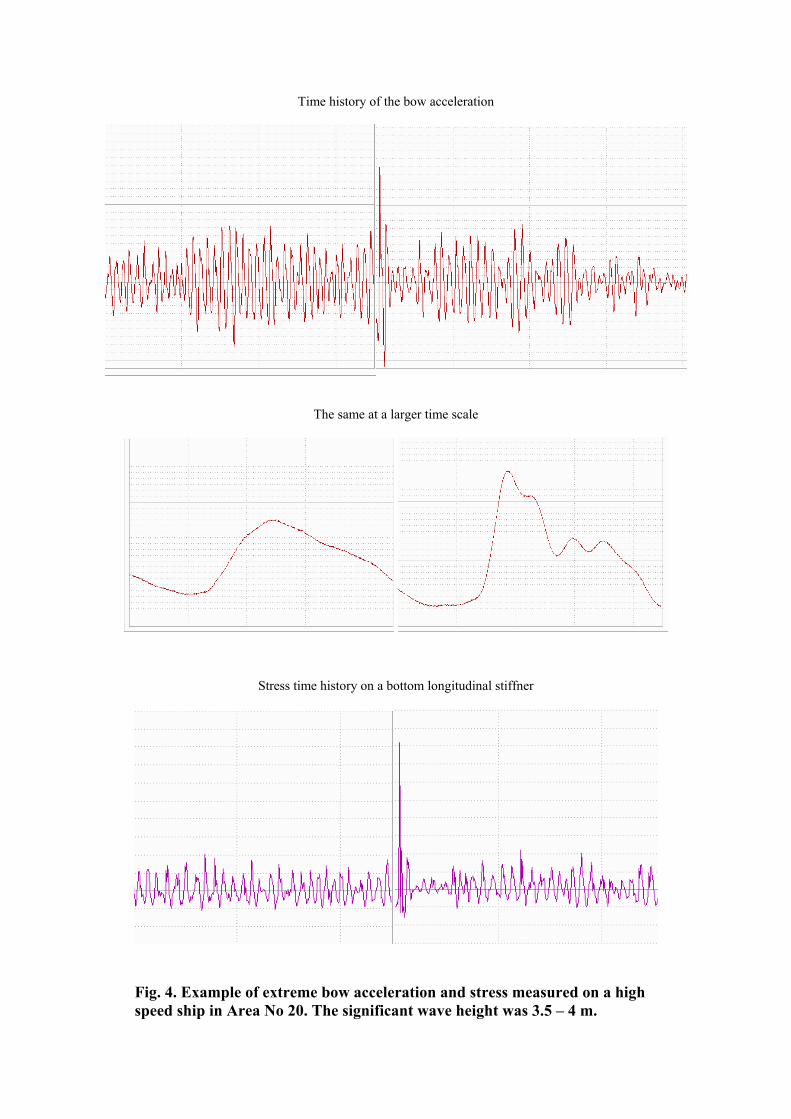
Time history of the bow acceleration
The same at a larger time scale
Stress time history on a bottom longitudinal stiffner
Fig. 4. Example of extreme bow acceleration and stress measured on a high
speed ship in Area No 20. The significant wave height was 3.5 – 4 m.

Fig. 5. Above left: A bimodal directional wave number spectrum. Right: A directional wave number spectrum showing wave-current refraction in the Gulf Stream. Freak waves have been measured in such directional seas. Below: A 3-dimensional shortcrested freak wave generated in laboratory experiments in order to simulate the wave shown in Fig. 1.

Fig. 6. Alltogether 8 capsizings has occurred in Area no 5 along the Norwegian coast and 29 people havelost their lives in these accidents. In this Area a warning for freak waves is initiated with success. Pyramidal waves of the kind shown in Fig 1 and Fig 5 can be observed here in severe weather conditions.

Fig. 7. Wave rays in severe weather conditions in the Area shown in Fig 6. A non-linear wave depth and wave current refraction takes place here. Depth contours are also shown.

Rogue waves and wave focusing – speculations on theory, numerical results and observations
Paul H Taylor
Department of Engineering Science
University of Oxford Oxford OX1 3PJ U.K.
This review will discuss recent work on the question of rogue waves on the open ocean. Observations of waves on the open sea are consistent with weakly non-linear modifications to a linear random process, at least most of the time even in violent storms1. The occurrence of large waves might then be attributable to the random alignment of many small independent components. Extracted from a random background, this process would then look like the linear focusing of an initially dispersed wave group. The focusing of uni-directional groups can produce dramatic extra surface elevation consistent with contraction of the group in the direction of motion. Simulations with the numerical scheme of Bateman2 with significant directional spreading show that much of the extra elevation is lost. However, considerable elongation of the group structure along the wave crests can occur. 2-D and 1-D evolution is also different in that, although the non-linear dynamics occur over a much shorter period in 2-D and require steeper waves for much to happen, the spectral content well after focus in 2-D is markedly different to that before even in the absence of wave breaking. For this type of focusing event, simple models based on the nonlinear Schrodinger equation reveal the importance of the Benjamin-Feir index in 1-D and suggest that directional spreading should be incorporated into the index. Recent work by Segur3 shows that the Benjamin-Feir instability is significantly affected by small amounts of dissipation. The review will end by pointing out that most work with phase resolved wave models neglects both energy input and dissipation. Does this invalidate our conclusions? References 1. Taylor, P.H. & Williams B.A. Wave statistics for intermediate depth water – NewWaves and symmetry. Journal of Offshore Mech. and Arctic Eng 126, 54. (2004) 2. Bateman, W.J.D., Swan, C. & Taylor, P.H. On the efficient numerical simulation of directionally spread surface water waves. Journal of Computational Physics, 174, 277 (2001). 3. Segur, H. Stabilizing the Benjamin-Feir Instability. Talk at Workshop on Free Surface Water Waves, held at the Fields Institute, Toronto, June 2004

The role of resonant wave interactions in theevolution of extreme wave events
Richard Gibson & Chris Swan
Department of Civil and Environmental EngineeringImperial College London
SW7 2AZUnited Kingdom
[email protected], [email protected]
Abstract. This paper is concerned with the formation of large wavesin a realistic, directionally-spread, wave-field. In particular, the role ofresonant interactions, capable of rapidly altering the underlying wave-spectrum, is ascertained. This is investigated through the use of a fully-nonlinear numerical wave-model and Zakharov’s evolution-equation. Theformer allows the full-nonlinearity of the wave-field to be considered,whilst the latter enables the physical mechanisms responsible for theformation of the largest waves to be determined. The paper shows thatin unidirectional sea-states the resonant interactions enable the forma-tion of waves that are very much larger than would be predicted bya second-order bound wave solution. However, it is also shown that inbroad-banded directionally-spread sea-states the effect of these interac-tions is linked to the phase relationship between the wave components;with significant spectral evolution only occurring when the wave compo-nents do not fully focus at one point in space and time. This suggeststhat the focussing of wave components is not a mechanism by whichso-called freak, or rogue, waves can form in a broad-banded directionalwave-field. However, large increases in crest elevation are obtained ina more narrow-banded directionally-spread sea-state, characterised bya Gaussian spectrum, and representative of swell wave conditions. Thepresent results suggest that it is in these conditions that freak waves aremost likely to occur.
1 Introduction
The water surface elevations arising in a realistic ocean environment are com-monly modelled by the sum of wave components, of different frequency, travellingin different directions. The constructive interference, or focussing, of these com-ponents at one point in space and time results in a large wave-event that isoften higher and steeper than linear, or second-order, bound wave theory wouldpredict. This is the result of the rapid evolution of the wave spectrum due toresonant interactions. As a result, the coupling of linear dispersion with nonlin-ear resonant interactions offers a possible explanation for the formation of freak

or rogue waves in deep water. This paper is concerned with the evolution of re-alistic wave spectra. In particular, it is concerned with the relationship betweenthe phasing of the wave components, the evolution of the wave spectrum and theresulting nonlinear crest elevation. This has been undertaken by applying twononlinear wave-models: Bateman et al. (2001) and Zakharov (1968). This paperbegins in §2 by describing the two wave-models. It continues in §3 by investigat-ing the evolution of both unidirectional and directional sea-states. Concludingremarks can be found in §4.
2 Wave Models
Two wave-models have been applied in order to model, and understand, the evo-lution of realistic directionally spread sea-states. The first is the fully-nonlinearnumerical wave-model of Bateman et al. (2001). The second is the evolution-equation of Zakharov (1968). Whilst the former solves the exact fully-nonlinearboundary conditions it gives very little direct indication as to the physical mech-anisms that govern the evolution of a sea-state. In contrast, Zakharov (1968) en-ables the interactions at each order to be separated and the dominant physicalprocesses to be determined.
Bateman et al. (2001) is an extension to three-dimensions of the unidirec-tional wave-model of Craig & Sulem (1993). It is applied by time-marching thesurface profile, η(x, y), and the velocity potential on that surface, ϕ(x, y), as firstsuggested by Zakharov (1968). At each time-step the horizontal derivatives ofthe surface, and of the velocity potential, can be rapidly calculated using fastFourier transform techniques. However, the calculation of the vertical derivativerequires the application of a Dirichlet-Neumann operator that transforms valuesof the potential on the surface into its vertical gradient. This is achieved by eval-uating a high-order Taylor series. This last step is the reason for the efficiencyof the Bateman et al. (2001) model; allowing realistic directional spectra, witha large range of frequencies, to be successfully modelled. In contrast, the wave-model of Johannessen & Swan (2003), itself an extension of the unidirectionalwave-model of Fenton & Rienecker (1982), solved for the unknown coefficientsusing large matrix inversion. This is computationally intensive, leading to aninefficient model incapable of describing realistic directional spectra.
In contrast, Zakharov (1968) is an integro-differential equation that has beenderived to fourth-order by Krasitskii (1994). At each order it is possible to isolatethe bound and resonant interactions that occur, and hence, it is an excellenttool for understanding the physical mechanisms that govern the evolution of awave-field. In this model the wave spectrum is time-marched according to whichinteractions are desired; making it possible to model the evolution of a wave-fieldincluding only the bound terms, only the resonant terms, or a mix of terms atdifferent orders. This allows the dominant physical processes to be isolated. Adetailed account of how it can be applied numerically is given by Annenkov &Shrira (2001), and a comparison with laboratory data is discussed in Shemeret al. (2001).

In order to investigate the evolution of large focussed wave-events the wave-models have been initiated with a specified wave spectrum at one point in time,t = t0, when the sea-state is dispersed. The phasing of the wave componentshas been determined on the basis of the linear dispersion relationship such thata perfectly focussed wave-event will occur at t = 0s. The wave-models are thentime-marched up to and beyond the largest crest elevation and the changes to thewave profile and the wave spectrum ascertained. In the Zakharov (1968) modelthe spectrum at each time-step is given in terms of the underlying linear wavecomponents. In contrast, the Bateman et al. (2001) model gives the spectrumof the surface profile, which inevitably includes bound terms. However, it ispossible to remove some of these bound terms by running the same cases so thata focussed wave trough occurs rather than a focussed wave crest. The troughfocussed wave profile is then subtracted from the crest focussed profile and theFourier transform of this result is a wave spectrum from which all the even-order(for example, second- and fourth-order) terms have been removed. However, odd-order terms are still present, and, although small, can potentially contaminatethe results.
3 Results
The fully-nonlinear model of Bateman et al. (2001) has been used to model theevolution of two unidirectional sea-states; both of which are characterised by aJONSWAP spectrum of peak period Tp = 12.8s. However, the two spectra dif-fer in their degree of broad-bandedness: the first has a peak enhancement factorγ = 1 (case J1D0) and the second a peak enhancement factor γ = 5 (case J5D0).Figure 1 shows that in both cases the fully-nonlinear wave profile of the extremewave-event has a crest elevation much larger than that predicted by the solutionof Zakharov (1968) that includes only the bound terms. Therefore, the formationof a large wave in a unidirectional sea-state cannot be modelled without takinginto account the evolution of the wave spectrum. Figure 2 shows the rapid evo-lution of the freely propagating wave components of cases J1D0 and J5D0. Inboth sea-states this analysis shows that the underlying linear spectrum broadensconsiderably during the evolution of an extreme wave-event. This broadening isassociated with an increase in the amplitude sum of the wave spectrum (Figure3), and hence, the broadening is responsible for the large increases in maximumcrest elevation. The physical mechanisms responsible for this evolution can bedetermined by applying Zakharov (1968). Indeed, figure 4 shows that an ex-cellent agreement between the two models can be found by including only thethird-order resonant terms. Furthermore, the evolution of these spectra is occur-ring much more rapidly than is predicted in random sea-states by Hasselmann(1962). The strong correlation between the phase of the wave components al-lows the third-order resonant interactions to broaden the wave spectrum overthe time-scale of tens of wave periods rather than hundreds. Whilst this is truefor unidirectional sea-states, in more realistic directionally spread wave-fieldsthese conclusions need revising.

−200 −150 −100 −50 0 50 100 150 200−4
−2
0
2
4
6
8
10
12
Location (m)
Ele
vatio
n (m
)
LinearSecond−orderThird−orderFully nonlinear
(a) J1D0
−200 −150 −100 −50 0 50 100 150 200−6
−4
−2
0
2
4
6
8
10
12
Location (m)
Ele
vatio
n (m
)
LinearSecond−orderThird−orderFully nonlinear
(b) J5D0
Fig. 1: Surface profile of extreme wave-events modelled using only the first-,second- and third-order bound terms of Zakharov (1968), and fully-nonlinearlyusing Bateman et al. (2001).
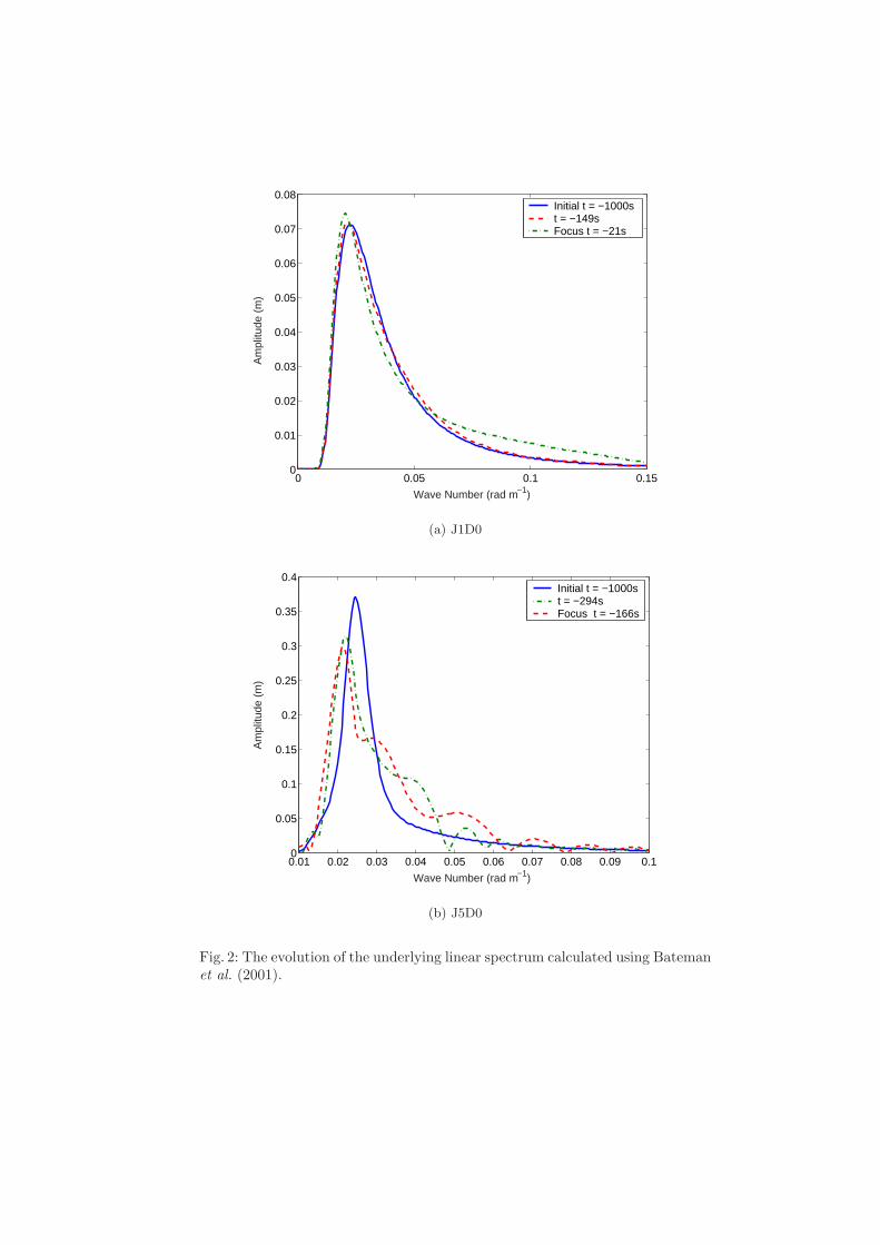
0 0.05 0.1 0.150
0.01
0.02
0.03
0.04
0.05
0.06
0.07
0.08
Wave Number (rad m−1)
Am
plitu
de (
m)
Initial t = −1000s t = −149s Focus t = −21s
(a) J1D0
0.01 0.02 0.03 0.04 0.05 0.06 0.07 0.08 0.09 0.10
0.05
0.1
0.15
0.2
0.25
0.3
0.35
0.4
Wave Number (rad m−1)
Am
plitu
de (
m)
Initial t = −1000st = −294sFocus t = −166s
(b) J5D0
Fig. 2: The evolution of the underlying linear spectrum calculated using Batemanet al. (2001).

−400 −300 −200 −100 0 1008.5
9
9.5
10
10.5
11
11.5
12
Time (s)
Am
plitu
de S
um A
(m
)
G1D0G5D0
Fig. 3: The amplitude sum of the underlying linear spectrum. The high frequencyoscillations represent third-order nonlinearites.
The fully-nonlinear model of Bateman et al. (2001) has also been used tomodel the evolution of two directional sea-states; both of which are characterisedby a JONSWAP spectrum of peak period Tp = 12.8s and peak-enhancement fac-tor γ = 5. However, the two spectra differ in their degree of directional spreading:the first corresponds to a wrapped normal distribution with a standard deviationof σθ = 5 (case J5D5), while the second has a standard deviation σθ = 30 (caseJ5D30). Figure 5 shows that in both cases the crest elevation associated withthe extreme wave profile is actually lower than that predicted by second-ordertheory. An analysis of the amplitude sum of the spectra (figure 6) indicates thatthe evolution of the amplitude spectra does not directly explain the reductionin crest elevation: in case J5D5 the amplitude sum increases from 9m to 11.6m;whilst, in case J5D30 it decreases from 9m to 8.7m. These changes to the am-plitude sum are directly related to changes in the bandwidth of the two spectra,with a broadening of case J5D5 and a narrowing of J5D30. The actual changesto the spectral shape are considered in more detail in Gibson & Swan (2005).However, it is clear that there is a further factor to consider in determining themaximum crest elevation.
The maximum crest elevation associated with an extreme wave-event at anypoint in time, te, is the product of four inter-related factors. The first is theamplitude sum of the underlying linear wave spectrum at the initial time, A0 =A|t=t0 =
∑Ni ai|t=t0 , where ai are the amplitudes of the wave components. The
second is the change to this amplitude sum due to resonant interactions ∆A. Thethird is the nonlinear correction due to bound interactions. Finally, the fourthis the phase relationship between the wave components. These factors are notindependent; for example, the bound correction depends upon the amplitude sumof the wave components and their phasing. Despite this, it can be informativeto investigate these factors in terms of a number of ratios:

0 0.05 0.1 0.150
0.2
0.4
0.6
0.8
1
Nor
mal
ised
Am
plitu
de
LinearBSTZE
(a) J1D0
0 0.02 0.04 0.06 0.08 0.10
0.2
0.4
0.6
0.8
1
Wave Number (rad m−1)
Nor
mal
ised
Am
plitu
de
InitialBSTZE
(b) J5D0
Fig. 4: Comparison between the evolution of the underlying linear spectrum cal-culated using Bateman et al. (2001) with that calculated using Zakharov (1968).All the results are from t = −100s.
ηactual = FA|t0 = F0F1F2A|t0 , where, (1)F0 = (∆A + A0)/A0 ,
F1 = ηbound/(∆A + A0) ,
F2 = ηactual/ηbound ,
and ηbound defines the crest elevation, including the effect of bound interactions, ifa perfectly focussed wave-event occurred, and ηactual is the actual crest elevation.Taking each in turn: F0 is the increase in the amplitude sum of the underlyinglinear wave components; F1 is the increase in the crest elevation due to boundinteractions, if the wave components are perfectly focussed; and F2 defines thefocal quality of the event.

−600 −400 −200 0 200 400 600−5
0
5
10
Location (m)
Ele
vatio
n (m
)
LinearSecond−orderThird−orderFully−nonlinear
−600 −400 −200 0 200 400 600−10
−5
0
5
10
15
Location (m)
Ele
vatio
n (m
)
LinearSecond−orderThird−orderFully−nonlinear
Fig. 5: Surface profile of extreme wave-events modelled using only the first-,second- and third-order bound terms of Zakharov (1968), and fully-nonlinearlyusing Bateman et al. (2001).
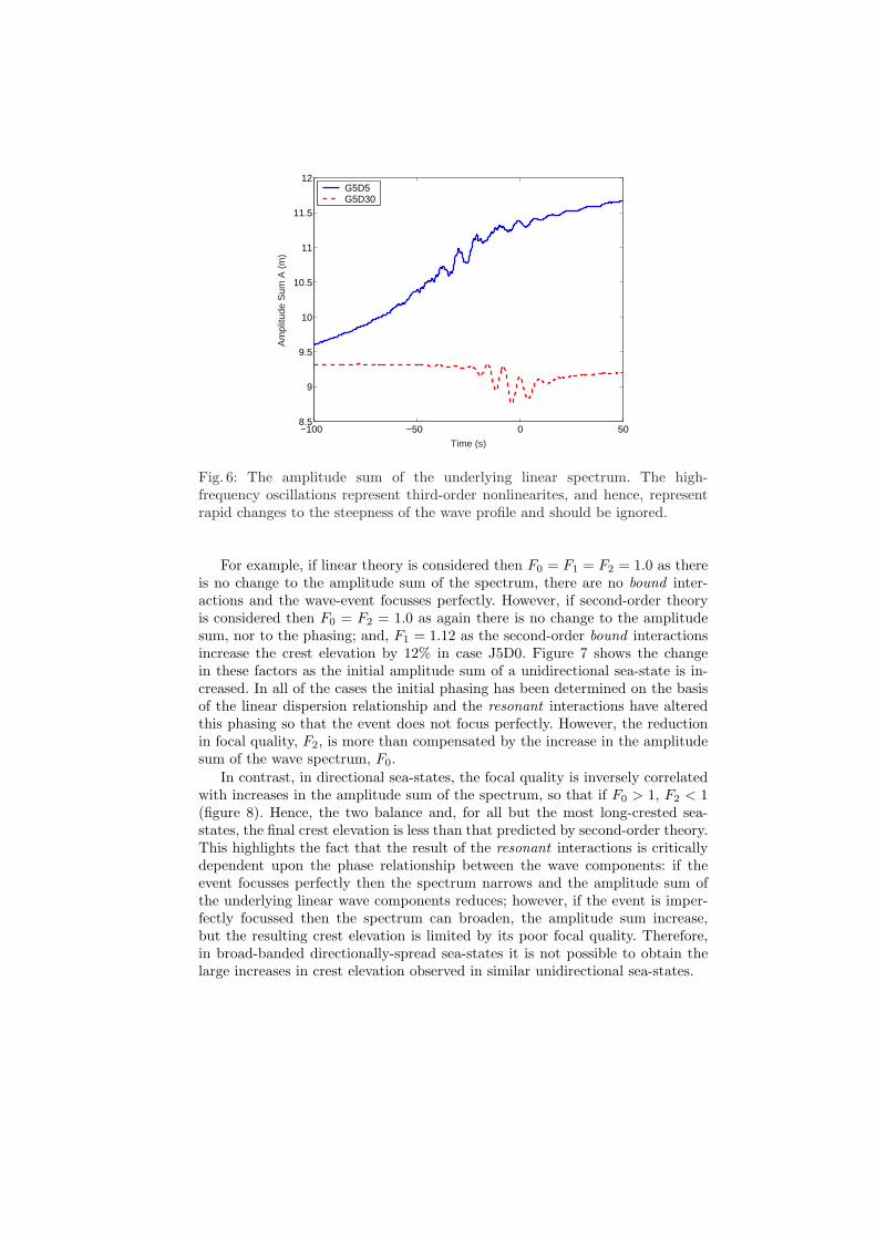
−100 −50 0 508.5
9
9.5
10
10.5
11
11.5
12
Time (s)
Am
plitu
de S
um A
(m
)
G5D5G5D30
Fig. 6: The amplitude sum of the underlying linear spectrum. The high-frequency oscillations represent third-order nonlinearites, and hence, representrapid changes to the steepness of the wave profile and should be ignored.
For example, if linear theory is considered then F0 = F1 = F2 = 1.0 as thereis no change to the amplitude sum of the spectrum, there are no bound inter-actions and the wave-event focusses perfectly. However, if second-order theoryis considered then F0 = F2 = 1.0 as again there is no change to the amplitudesum, nor to the phasing; and, F1 = 1.12 as the second-order bound interactionsincrease the crest elevation by 12% in case J5D0. Figure 7 shows the changein these factors as the initial amplitude sum of a unidirectional sea-state is in-creased. In all of the cases the initial phasing has been determined on the basisof the linear dispersion relationship and the resonant interactions have alteredthis phasing so that the event does not focus perfectly. However, the reductionin focal quality, F2, is more than compensated by the increase in the amplitudesum of the wave spectrum, F0.
In contrast, in directional sea-states, the focal quality is inversely correlatedwith increases in the amplitude sum of the spectrum, so that if F0 > 1, F2 < 1(figure 8). Hence, the two balance and, for all but the most long-crested sea-states, the final crest elevation is less than that predicted by second-order theory.This highlights the fact that the result of the resonant interactions is criticallydependent upon the phase relationship between the wave components: if theevent focusses perfectly then the spectrum narrows and the amplitude sum ofthe underlying linear wave components reduces; however, if the event is imper-fectly focussed then the spectrum can broaden, the amplitude sum increase,but the resulting crest elevation is limited by its poor focal quality. Therefore,in broad-banded directionally-spread sea-states it is not possible to obtain thelarge increases in crest elevation observed in similar unidirectional sea-states.

1 2 3 4 5 6 7 8 9 100.9
0.95
1
1.05
1.1
1.15
1.2
1.25
1.3
1.35
1.4
Initial Amplitude Sum (A0)
Rat
io
F0 (Resonant interactions)
F1 (Bound interactions)
F2 (Focal quality)
F (Nonlinear amplification)
Fig. 7: The factors that effect the crest elevation of an extreme wave-event in aunidirectional sea-state.
0 5 10 15 20 25 300.7
0.8
0.9
1
1.1
1.2
1.3
1.4
Spreading Parameter (σn)
Rat
ios
F0 (Resonant interactions)
F2 (Focal quality)
F (Nonlinear amplification)
Fig. 8: The factors that effect the crest elevation of an extreme wave-event in amulti-directional sea-state characterised by a JONSWAP spectrum with a peak-enhancement factor γ = 5.0.

However, whilst it is not possible to obtain large increases in crest elevationif the spectrum is broad-banded, it is possible in more narrow-banded sea-states.Bateman et al. (2001) has been used to model the evolution of a Gaussian sea-state with a small directional spread of σn = 5, characteristic of swell waves.In this case the sea-state disperses slowly, and the balance between changes tothe spectral bandwidth due to resonant interactions and the focal quality of theextreme-event is balanced towards the former. Figure 9 shows that the maximumcrest elevation is much larger than that predicted by a bound wave solution. Ittherefore follows that, swell-dominated sea-states are perhaps those in whichrogue waves are intrinsically more likely to occur.
−400 −300 −200 −100 0 100 200 300 400−10
−5
0
5
10
15
Location (m)
Ele
vatio
n (m
)
LinearSecond−orderThird−orderFully−nonlinear
Fig. 9: Surface profile of an extreme wave-event in a swell-dominated sea-state,characterised by a Gaussian spectrum with a spreading parameter σn = 5.
4 Concluding Remarks
The fully-nonlinear evolution of both unidirectional and directional sea-stateshas been investigated. It has been shown that in the former third-order resonantinteractions lead to the rapid evolution of the wave spectrum, and to an increasein the crest elevation of an extreme wave-event. Whereas, in the latter the ex-treme crest-elevation is less than that predicted by second-order theory. Thisreduction is due to the balance between the phasing of the wave componentsand the spectral changes that occur during the formation of a large event. Thissuggests that the focussing of wave components is not a possible mechanismby which rogue waves can form in broad-banded sea-states. However, in morenarrow-banded Gaussian spectra, characteristic of swell-dominated sea-states,

large waves are slow to disperse. Hence, the balance is now in favour of the res-onant interactions and large increases in crest elevation can be obtained.
Acknowledgement
The early stages of this work were undertaken within the project ‘ReliabilityBased Structural Design of FPSO Systems’, which involves Shell International,Instituto Superior Tcnico, DHI, Det Norske Veritas, Imperial College, NobleDenton and Oxford University. The project is partially funded by the EuropeanUnion through the Energy Programme under contract ENK6-2000-00107. Thelater stages of the work were completed with support from the UK Engineeringand Physical Sciences Research Council under grant number GR/R64971.

Bibliography
Annenkov, S. & Shrira, V. 2001 Numerical modelling of water-wave evo-lution based upon the zakharov equation. Journal of Fluid Mechanics 449,341–371.
Bateman, W. J. D., Swan, C. & Taylor, P. H. 2001 On the efficient numer-ical simulation of directionally-spread surface water waves. Journal of Com-putational Physics 174, 277–305.
Craig, W. & Sulem, C. 1993 Numerical simulation of gravity waves. Journalof Computational Physics 108, 73–83.
Fenton, J. D. & Rienecker, M. M. 1982 A fourier method for solving non-linear water-wave problems: application to solitary-wave interactions. Journalof Fluid Mechanics 118, 411–443.
Gibson, R. S. & Swan, C. 2005 The evolution of large ocean waves: the roleof local and rapid spectral changes.. Submitted to the Royal Society .
Hasselmann, K. 1962 On the nonlinear energy transfer in a gravity wave sys-tem. Part 1. Journal of Fluid Mechanics 12, 481–500.
Johannessen, T. B. & Swan, C. 2003 On the nonlinear dynamics of focusedwave groups in two and three dimensions. Proc. Roy. Soc. Lond. A 459, 1021–1052.
Krasitskii, V. P. 1994 On reduced equations in the hamiltonian theory ofweakly nonlinear surface waves. Journal of Fluid Mechanics 272, 1–20.
Shemer, L., Jiao, H., Kit, E. & Agnon, Y. 2001 Evolution of a nonlinearwave field along a tank: experiments and numerical simulations based uponthe spatial zakharov equation. Journal of Fluid Mechanics 427, 107–129.
Zakharov, V. E. 1968 Stability of periodic waves of finite amplitude on thesurface of a deep fluid. Journal of Applied Mechanics and Technical Physics9, 190–194, english Translation.

Experimental study of the wind effect
on the focusing of transient wave groups
J.P. Giovanangeli1), C. Kharif1) and E. Pelinovsky1,2)
1)Institut de Recherche sur les Phénomènes Hors Equilibre, Laboratoire IRPHE/IOA, Marseille, France. Email: [email protected] 2)Laboratory of Hydrophysics and Nonlinear Acoustics, Institute of Applied Physics, Nizhny Novgorod, Russia. Email: [email protected]
One of the popular mechanisms of the freak waves phenomenon is the dispersive focusing of
transient wave groups. In all published theoretical and experimental papers the surface gravity
waves are considered as an ensemble of free waves. This paper reports on a series of experiments
conducted in the large wind-wave tank of IRPHE (Marseille – Luminy) to study the wind effect on
the generation of freak waves. A suitable theory is presented to explain and discuss the
experimental results.
1. Introduction
Freak wave phenomenon is now explained by many physical theories: dispersive and
geometrical focusing, nonlinear modulational instability (Benjamin – Feir instability), wave-
current and wave-bottom interactions; see, for instance (Olagnon and Athanassoulis, 2001;
Rogue Waves, 2003; Kharif and Pelinovsky, 2003). In all published theoretical and
experimental papers the gravity waves on sea surface are assumed to be an ensemble of free
waves. In early stages the wind flow is considered as the source of the spatial and temporal
inhomogeneity of the wind wave field or as the factor of wave amplification. The present
paper reports on a series of experiments with transient wave groups under wind action up to
10 m/s conducted in the large wind-wave tank of IRPHE (Marseille – Luminy). Theoretical
model to explain the experimental results is developed. It includes the sub-surface current
induced by wind. The theoretical predictions are in good agreement with experimental results.
2. Set-up and experimental conditions
The experiments have been conducted in the large wind-wave tank of IRPHE at Marseille -
Luminy (Figure 1). It is constituted of a closed loop wind tunnel located over a water tank
40m long, 1 m deep and 2.6 m wide. The wind tunnel over the water flow is 40 m long, 3.2 m
wide and 1.6 m high. The blower allows to produce wind speeds up to 14 m/s and a computer-
controlled wave maker submerged under the upstream beach can generate regular or random

waves in a frequency range from 0.5 hz to 2 Hz. Particular attention has been taken to
simulate pure logarithmic mean wind profile with constant shear layer over the water surface.
A trolley installed in the test section allows to locate probes at different fetches all along the
facility. The water surface displacements were determined by using three capacitive wave
gauges of 0.3 mm outer diameter with DANTEC model 55E capacitance measuring units.
Two wave gauges was located at fixed fetches of 1m and 3 m from the uspstream beach. A
third wave gauge was installed on the trolley in order to determine the water surface
deflections η at various distances from the upstream beach. The typical sensitivity of the wave
probes was of order of 0.6 V/cm.
Figure 1: A schematic representation of the Large Air-Sea Interactions Facility.
For each value of the mean wind speed, W equals to 0, 4, 5, 6, 8 and 10 m/s, the water surface
deflections η was measured at 1 m fetch and at different fetches between 5m and 35 m. The
wave maker was driven by an analog electronic signal varying linearly with time from 1.3 Hz
to 0.8 Hz in 10 seconds with constant amplitude of displacements corresponding to nearly
constant amplitude of the initial wave group. The fetch values are taken from the entrance of
the wave-tank, where the airflow meets the water surface i.e. at the end of the upstream beach.
Typical value of σ equal to the rms of the water deflections η determined at the distance 1 m
for different wind speeds is 1.87-1.88 cm.
3. Experimental Results
Figure 2 demonstrates the focusing of the free transient wave groups when there is no wind
flow above waves. Initial wave packet has the step-wise amplitude modulation and linearly
frequency modulation. As predicted by the linear theory of the free deep-water waves, the
waves focused at a precise distance, leading to the occurence of a high amplitude freak wave.
Downstream of the point of focusing, the amplitude of the group decreases rapidly
(defocusing). The influence of the wind flow with speed 6 m/s on the wave focusing process
is shown in Figure 3. The characteristics (frequencies and amplitude) of the initial
mechanically generated waves are kept the same. As it can be seen, the scales of spatial -

temporal evolution of the group are changed with wind. For each value of the wind speed, the
amplification ratio A(X,W) can be defined as A = ηmax/σ, where ηmax is the maximum
amplitude of the wave packet on fixed distance. Figure 4 gives the amplification ratio as a
function of the distance from the upstream probe located at 1 m fetch and for different values
of the wind speed. This figure shows that in presence of wind, we observed a freak wave of a
larger amplitude, occuring at a longer distance than observed without wind. Moreover,
contrarely to the case without wind, the freak waves maintains its coherency and its amplitude
as it propagates downstream the previous focusing point. The effects of wind on the location
of the focusing point, on the amplitude and the coherency of the freak wave increases as the
wind velocity increases.
0 5 10 15 20 25 30 35 40 45 50-10
0
10
20
30
40
50
s
Fe tch 3m
Fe tch 3m
Fe tch 3m
Fe tch 3m
Fe tch 3m
Fe tch 22m
Fe tch 24m
Fe tch 26m
Fe tch 29m
Fe tch 31m
0 5 1 0 1 5 2 0 2 5 3 0 3 5 4 0 4 5 5 0-1 0
0
1 0
2 0
3 0
4 0
5 0
s
F e tc h 3 m
F e tc h 3 m
F e tc h 3 m
F e tc h 3 m
F e tc h 3 m
F e tc h 1 2 m
F e tc h 1 4 m
F e tc h 1 6 m
F e tc h 1 8 m
F e tc h 2 0 m
Time, s
dis
pla
cem
ent,
cm
Figure 2: Time series of the water surface displacement, η on various distances from the wave paddle
(no wind); initial packet is shown on the left

0 5 10 15 20 25 30 35 40 45 50-10
0
10
20
30
40
50
ta cms
Fetch 12 m Fetch 8 m
Fetch 14 m
Fetch 16 m
Fetch 18 m
Fetch 20 m
Fetch 3 m
Fetch 3 m
Fetch 3 m
Fetch 3 m
0 5 10 15 20 25 30 35 40 45 50-10
0
10
20
30
40
50
s
Fe tc h 3 m
Fe tc h 3 m
Fe tc h 3m
Fe tch 3 m
Fe tc h 3 m
Fe tc h 22 m
Fe tch 2 3 m
Fe tch 25 m
Fe tch 27 m
Fe tch 29 m
Time, s
dis
pla
cem
ent,
cm
Figure 3: Time series of the water surface displacement, η on various distances from the wave paddle, wind speed 6 m/s; initial packet is shown on the left
0 10 20 30 40Distance, m
1
2
3
4
5
Am
plif
icat
ion
04568
Figure 4: Amplification ratio versus the distance from the wave paddle for various wind speed

Results of the wavelet analysis of time series of the surface elevation at 3 m and 25 m for
wind speed 8 m/s are presented in Figure 5. These figures show the time frequency evolution
of the group as it propagates downstream along the wave tank. As it can be seen, the wind
generated ripples have other frequencies than the transient group.
Figure 5: Wavelet analysis of the time records for wind speed 6 m/s
Clearly Figure 5 shows the wind waves are damped by the freak wave. This result is of the
first importance for remote sensing.
4. Focusing of narrow-banded wave groups
The dynamics of narrow-banded linear wave packets can be described by the parabolic
equation for wave amplitude
2
2
20
0
8 xA
kxAc
tAi gr ∂
∂=
∂∂+
∂∂ ω , (1)
where k0 and ω0 are the wave number and frequency of the carrier wave, cgr = dω/dk is the
group velocity. The wave amplitude, A, is a slowly varying function of x and t.
Let us consider first the wave transformation of the wave packets with no wind. Transforming
the variables into dimensionless form

)/(0 grcxt −=ωτ , xky 0= , Aka 0= , (2) equation (1) can be re-written as spatial parabolic equation
2
2
τ∂∂=
∂∂ ayai , (3)
which should be completed by the boundary condition on the paddle
)()0,( ττ fya == . (4)
Equation (1) or (3) are widely used to demonstrate the effect of the wave focusing of the
linear transient groups (Clauss and Bergmann, 1986; Pelinovsky & Kharif, 2000; Brown &
Jansen, 2001). In particular, if the boundary condition (4) corresponds to the packet with
amplitude modulation of gaussian shape
( )22
00 exp)0,( ττ Ω−= Aa , (5) in the process of the wave evolution its complex envelope is described by
Ω−
Ω−Ω−
=yiyi
Aya 20
220
20
0
41exp
41),( ττ , (6)
and, as a result, the wave has a variable amplitude and phase (frequency) modulation. The
variation of the amplitude of the wave packet is
[ ]
Ω+
Ω−Ω+
= 240
220
4/1240
0
161exp
161|),(|
yyAya ττ . (7)
At each point the amplitude modulation presents a gaussian profile in time, and its peak value
decreases on large distance as y-1/2
[ ] 4/1240
0max
161||
yAaΩ+
= . (8)
The characteristic width of the amplitude modulation is
0
240161
)(Ω
Ω+=
yyT (9)
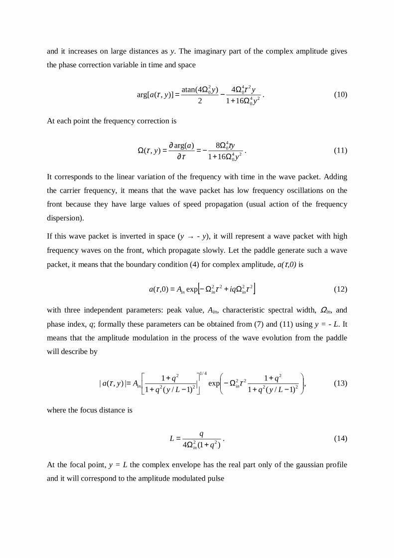
and it increases on large distances as y. The imaginary part of the complex amplitude gives
the phase correction variable in time and space
240
240
20
1614
2)4(atan)],(arg[
yyyya
Ω+Ω−Ω= ττ . (10)
At each point the frequency correction is
240
40
1618)arg(),(
yyay
Ω+Ω−=
∂∂=Ω τ
ττ . (11)
It corresponds to the linear variation of the frequency with time in the wave packet. Adding
the carrier frequency, it means that the wave packet has low frequency oscillations on the
front because they have large values of speed propagation (usual action of the frequency
dispersion).
If this wave packet is inverted in space (y → - y), it will represent a wave packet with high
frequency waves on the front, which propagate slowly. Let the paddle generate such a wave
packet, it means that the boundary condition (4) for complex amplitude, a(τ,0) is
[ ]2222exp)0,( τττ ininin iqAa Ω+Ω−= (12)
with three independent parameters: peak value, Ain, characteristic spectral width, Ωin, and
phase index, q; formally these parameters can be obtained from (7) and (11) using y = - L. It
means that the amplitude modulation in the process of the wave evolution from the paddle
will describe by
−+
+Ω−
−+
+= 22
222
4/1
22
2
)1/(11exp
)1/(11|),(|
Lyqq
LyqqAya inin ττ , (13)
where the focus distance is
)1(4 22 qqL
in +Ω= . (14)
At the focal point, y = L the complex envelope has the real part only of the gaussian profile
and it will correspond to the amplitude modulated pulse

( )22exp),( ττ ffALa Ω−= , [ ] 4/121 qAA inf += , [ ] 2/121 qinf +Ω=Ω . (15) The solution given above describes the evolution of a free transient group with the formation
of a freak wave. Results of the comparison with experimental data are presented in Figure 6.
We used the following parameters: Af = 3.8 m, f0 = 1 Hz and Ω0 = 0.062. In the case of no
wind the agreement between theoretical and numerical results is quite good.
0 10 20 30 40Distance, m
1
2
3
4
5
Am
plif
icat
ion
0
Figure 6: Comparison between experimental points and solution of the parabolic equation The next step is to include the wind effect. The wind leads to the wind increment and also the
induced flow. As it is known, the linear part of the any evolution equation is the inverse
Fourier transformation of the linear dispersion relation. The induced flow modifies the
dispersion relation which can be written as follows
2
2 1414
−+=
gu
ugk ω . (166)
Then, the wave number should be developed by using Taylor series in the vicinity of the
carrier frequency, ω0
...)(21)( 2
02
2
00
00
+−+−+= ωωω
ωωω ωω d
kdddkkk , (17)
where k0 and ω0 satisfy the dispersion relation (16), and two important coefficients in (17)
equal to

+−=
guud
dk
041
111
0ωω ω
, 2/3
02
2 412
0
−
+=
gu
gdkd ω
ω ω
(18)
When the flow is absent, these coefficients transform into known formulas
gddk 02
0
ωω ω
= , gd
kd 2
0
2
2
=ωω
, (19)
which are the inverse group velocity and inverse dispersion parameter. The evolution equation
can be easily obtained from (17) considering i(k – k0) and –i(ω - ω0) as the differential
operators ∂/∂x and ∂/∂t (in fact, coordinate and time are slow variables of the wave envelope)
2
2
2
2
021
τω ω ∂∂=
∂∂ A
dkd
xAi , (20)
where τ = t – x/cgr. Equation (20) reduces to (3) when the current vanishes. The wind
increment can be introduced by adding a linear term
isAAd
kdxAi +
∂∂=
∂∂
2
2
2
2
021
τω ω
. (21)
This lattert term responsible of the wind generation can be eliminated by
)exp(),(),( sxxBxA ττ = , (22)
and finally we obtain again a parabolic equation
2
2
2
2
021
τω ω ∂∂=
∂∂ B
dkd
xBi . (23)
Equation (23) was investigated earlier and we may use the previous gaussian solution (by
replacing the coefficients) to study the wind effect. First of all, some conclusions can be done
before any procedures. As it is evident, the wind increment modifies the wave amplitude
providing additional growth of the wave field, but really this effect is not important; see
Figure 5. The second one is that the group velocity (dω/dk) increases with the current and,
therefore, the focal point will be shifted on large distance from the paddle. The third one is

that the dispersion parameter (d2k/dω2) decreases with the current and, therefore, the wave
amplitude will change more slowly with distance. All these conclusions correspond to the
experimental data and may be illustrated by the gaussian solution again. If the wave envelope
in the focal point is the gaussian pulse
( )22
0 exp)0,( ττ Ω−= Aa (24) (now we use dimensional variables), the maximal amplitude will vary with distance as
[ ] 4/1242220
max)()/(41
||Lxdkd
Aa−Ω+
=ω
. (25)
Figure 7 shows the comparison with observed data for wind speed value 4 m/s. Here we used
experimental values for envelope in the focal point: A0 = 3.8 m, Ω = 0.98 Hz. The comparison
is quite good.
0 10 20 30 40Distance, m
1
2
3
4
5
Am
plif
icat
ion
4
Figure 7: Comparison between predictions of linear parabolic equation and experimental data for wind speed 4 m/s However, in presence of wind, the assymetry observed on the curve is not found by the
model. Reul et al , 1999 have shown that over a steep wave, air flow separation process can
occur inducing large local enhancement of the momentum flux from wind to the wave. We
therefore could suggest that this process could occur in the same manner over the rogue wave
at and downstream the focusing point. This could maintain the freak as it propagates after the
focusing point.

5. Conclusion
The focusing of the transient wave groups under a wind flow action has been investigated
experimentally and theoretically. It is shown that focal distance is increased as well as the
maximum wave amplitude in this point. This effect is explained by the kinematic (Doppler)
effect in the dispersion relation in the framework of the parabolic equation.
This research is supported by CNRS and for EP by FRBR (05-05-64265) and INTAS (03-
514286).
References
Brown M.G., Jensen A. Experiments on focusing unidirectional water waves. J. Geophys. Resarch,
2001, vol. 106, N. C8, 16917 – 16928.
Clauss G., Bergmann J. Gaussian wave packets: a new approach to seakeeping tests of ocean
structures. Applied Ocean Research, 1986, vol. 8, 190-206.
Kharif C., Pelinovsky E. Physical mechanisms of the rogue wave phenomenon. European Journal
Mechanics / B – Fluid, 2003, 22, 603-634.
Olagnon M., Athanassoulis G.A. (Eds.), Rogue Waves 2000. France: Ifremer, 2001.
Pelinovsky E., Talipova T., Kharif, C. Nonlinear dispersive mechanism of the freak wave formation
in shallow water. Physica D, 2000, vol. 147, N. 1-2, 83-94.
Rogue Waves: Forecast and Impact on Marine Structures. GKSS Research Center, Geesthacht,
Germany, 2003.
Reul N., H. Branger and Giovanangeli J.P. Air flow separation over unsteady breaking waves.
Physics of Fluids, 1999, Vol 11, N.7, 1959-1961

Rogue Waves 2004 Workshop, Brest, France
A rapid fully nonlinear method in three dimensionswith simulations of steep wave event.
D. Fructus and J. Grue
Mechanics Divison, Department of Mathematics, University of Oslo, Norway
Introduction
An efficient numerical scheme for simulations of fully nonlinear non-breaking surfacewater waves is presented. The water depth is either finite or infinite and the bottomis allowed to be varying in time and space. The method is based on a fast, rapidlyconverging, iterative algorithm to compute the Dirichlet to Neumann operator. Thisis evaluated by expanding the operator as a sum of global convolution terms and localintegrals with kernels that decay quickly in space. The global terms are computed veryquickly via FFT. The local terms are evaluated by numerical integration. Analyticalintegration of the linear part of the prognostic equations is combined with a special stepsize control technique. This yields a very stable and accurate time marching procedure.Zeros-padding in the spectral space represents the anti-aliasing strategy. The methodrequires no smoothing. The scheme is stable and accurate, even for very long timesimulations of very steep wave events. The scheme is easily parallellizable. Illustrationthrough examples are considered. In a first simulation, the bottom is varying in time.In a second one, where the water depth is infinite, the focus is put uppon long timeevolution of wave group leading to the generation of rogue wave.
Fully nonlinear numerical model
We consider three-dimensional irrotational wave motion at the surface of a homo-geneous incompressible fluid over a horizontal impermeable bottom.
x=(x, y), z, denotes horizontal and vertical coordinates. z=0, z=−h and z=η(x, t)are, respectively, the equations of the still level, of the impermeable bottom and of thefree surface. Let also ~v = (u, w) be the velocity field, where u = (u, v) and w are thehorizontal and vertical velocities, so that ~v =grad φ. u=∇φ and w =φz; φ being thevelocity potential and ∇ being the horizontal gradient. We denote with ‘tildes’ thequantities at the free surface, e.g. φ(x, t) = φ(x, z = η(x, t), t). At the free surface, u
and w are expressed by,
u =∇φ − V ∇η +
(
∇η ×∇φ)
×∇η
1 + |∇η|2, w =
V + ∇η · ∇φ
1 + |∇η|2,
V =φn
√
1+|∇η|2
The kinematic and dynamic conditions give at the surface
ηt − V = 0, φt + gη + u · ∇φ − w V = 0.
The Laplace equation (resulting from incompressibility and irrotationality), togetherwith the bottom impermeability, is solved exactly by means of a Green function and themethod of images. For simplicity, we present here the deep water case only (h=const.=
1

∞). The generalization to an arbitrary bottom (allowed to be varying in time andspace) will be as well presented.
The Fourier transform of V , F(V ) = V is then decomposed into
V = V1 + V2 + V3 + V4.
The equation is inverted to give (in deep water):
V1 = k φ,
V2 = −kF η V1 − ik · F
η∇φ
,
2πV3 = kF
∫
φ′
[
1 − (1 + D 2)−32
]
∇′ ·[ (η′ − η)∇′R−1] dx′
,
2πV4 = −πkF η2 F−1kFV − 2ηF−1kFηV + F−1kFη2V
+kF
∫
V ′ R−1
[
1 − D 2 − (1 + D 2)−12
]
dx′
.
Where R = |x′−x| and D = (η(x′, t)−η(x, t))/R = (η′−η)/R. The kernels of theinner integrals of V3 and V4 decay like R−4 and R−5, respectively. These integrals areevaluated over a very limited region of the x-plane. V4 is determined implicitly andhence computed iteratively, for practical computations one iteration is sufficient. Themethod is shown to be very fast, accurate and stable without requiring any smoothing.
Applications
We present two examples of application of the method. The first simulation illus-trates the method with an arbitrary bottom which is varying in time and space. Asudden collapse of the bottom generates waves that propagates at the surface of thefluid, this is illustrated in figure 1-a. A second simulation presents the evolution ininfinite depth of a modulated wave. Modulational instability build up to generate arogue wave. This is examplified in figure 1-b.
0 2 4 6 8 10 12 14 16−1.2
−1
−0.8
−0.6
−0.4
−0.2
0
0.2
x/h
η
a) b)
Figure 1: a): Wave elevation (- -) resulting from a sudden collapse of the bottom (–).b): Fully nonlinear simulation of a rogue wave event with the present model.
References
Clamond and J. Grue, J. Fluid Mech., 2001, 447, 337.J. Grue, Applied Ocean Res., 2002, 24, 261-274.D. Fructus, D., Clamond, J., Grue & Ø. Kristiansen, 2004, sub. to J. Comp. Phys.
2

!#"%$& ' ()$* +$-, .-, /01323457698:;=<?>#@7A38CBED8A35BGFH:ICJK>#LFNMFH;O8QP0RSA3TU2V5MW< A35MXP048CFNIYFHA35(Z4A38CF\[]J
< @7;OB^4A35FNBGI_LFN`aFHIFH2V5b>L;GcAd8YTU;G5eYQ23[f@XAdYC4;GTgAdYCFHBGIO>h_5FN`V;O8CFNIYjik23[*lICRH2>m_238n0AoiJ_p 5IYF\Y:YqM;ErQ;GB^4;O8CB^4;sIC:8QRN;GIQt*4 u;G52VT7v;O5;GI_w_238CIqx*ya:FHRHFNz8C;d>#@XA38IC;OFHRHRN;3>D#8CA35BO;|/~~W~g-a~&4;9RH2V5YCFHTU;;?`V2VRN:YFN2V5k23[/RH2V5n0AK`V;EcA3B^d;OYIQnQ4FNB^4
ICcRHFNYFH5eY2A5:TzW;G8k2d[s;O5e`V;GRN2VcW;I2VRHF\Y2V5IFHIIY:MFH;GM.4;ICcRHFNYj:cc8C2aBG;OICIFHIk4FNV4R\i52V5RHFH5;KA38O>fnQFNY4RN2BGA3RHR\i`3;G8i4FHV4IY;G;Ocn0AK`V;OIzW;GFH5[]238CTU;GMb> ;O`3;G5¡FN[QY4;FN5FNYCFSA3R*n0Ao`3;ICRN2VcW;FHI8A=Y4;O8qITAdRHR¢&4;9FH5F\YFSAdR£IY^AdYC;s23[Y4;9n0AK`V;9¤;GRNM7FNIICcW;GBOFN¤;OMXFH5kYjn 2gIY;OcIG D&FH8IYA35; ¥AdBOY¦IYC;KA3Mi§aYC2V3;OI¦n0AK`V;d>!nQF\Y4+n0Ao`3;G5:TzW;G8¨V©¦A35MA3TUcRNFNY:M;ªe©(«4A3RN[YC4;Y23YA3Rn0Ao`3;4;OFHV4eY ¬QFHIqBG2VTUc:YC;GMb§;OBG2V5MRNiV>#Y4;IC:8[A3BO;;GRN;O`dAdYFN2V57A35MXYC4;sYA35V;O5YCFSA3R-`3;GRH2aBGF\YjiAdYsY4;I:8[AdBG;A38;T:R\YFNcRHFN;GMziY4;¯®°zW;GRNR¢±-[]:5B?YFH235+IC;OB^47²?³C©b´ µ*ªe© ¨ J© «d¶g·¶#©b¬a¸nQ4;G8;Y4;cA38AdTg;?Y;G8&³C© M;OYC;G8TgFN5;GIfYC4;¹RH;O53YC4º23[#Y4;0n0AK`V;QcA3B^d;OYG*»5¦;?¥A3B?Y IC2VRNFNY235IC23RH:YCFH2V52d[Y4;q52V5RHFN5;KAd8 §B^48K¼2VMFH5V;G8 ;Gy:A=YFH235X«m½§¬fFHI*23zY^A3FN5;GMºnQF\Y4U³C©¾¿V&»_5gFN5FNYCFSA3RaBG2V5MFNYCFH2V5nQFNYC4Uª©?¨V© ¾ÁÀÂÃÀVÄ9A35MU³C©¹¾ÅÀ°µ3ÆFHI*FN5c:Y*YC2EA[]:RHRNis52V5RHFH5;KA38fTU2aM;GR«P0RSA3TU2V5M¦Ad5Mg698:;3>µ3ÀVÀ¿Ç¬?
4;UBG2VTUc:YAdYFN2V5A3R&M2VTgA3FH5ÈFN5`32VRN`3;GIU¿Çµ3Én0Ao`3;GRN;G53YC4IAd5MÊYC4;¦BKA388CFH;O8n¹AK`V;gFHIMFNIBG8;OYCFHËG;OMÁ2o`V;O8¯Ìeµ52aM;GI7c£;O8(n0AK`V;ORH;G53Y4bÍ4FHI(Tg;GA35IY4AdY7A3RNR4A38Tg2V5FHBGIk:cÁY2Y4;¿ÇÎ=YC4A38C;8C;GI2VRN`3;GMb>A35MÏYC4AdY¿ÇµdÉD2V:8CFN;G87Tg2aM;GI¯A38C;+FN5BGRN:M;OMÐFH5ÁYC4;+ICcW;GB?Y8CA3RzA35MÑ ¨e©/· <J ¨V©KÒ^¨e©bÓ <J ¨V©CÔ¢*4;[]:RHR\ig52V5RHFN5;KAd80ICFNT:RHAdYFN2V5I IC42onÅY4AdY Y48;G;RHA38CV;qn¹AK`3;E;?`V;O5YCI2aBGBG:8M:8FH5¯YC4;kÌVÀVÀ3ÀXn¹AK`V;cW;G8FH2aMI23[qIFHT:RHAdYFN2V5b5:Tz£;O8º2V5;kAdYÕÖ=ש¾Ø¿oÎVÎ(n0Ao`3;cW;G8CFN2MI«¨V©ÙdÚ¾ÏÀ°µ3ÉVÆVÆ>W¨aÙdÚ¾ÏÀ°ÌdÛ¦¹¨YC4;ERH2aBKA3Rbn0AK`V;G5:Tz£;O8_!nQ4FHB^47FHIY4;sTAÇ¥FNTAdRn0Ao`3;k;GRN;O`dAdYFN2V523zIC;O8`V;OM¡M:8CFN5XY4;BG2VTUc:YAdYFN2V5I¬?>&5:Tz£;O8Yjn02A=YÕÖ=×£©g¾ÜÛ¿KÀ(n0Ao`3;cW;G8CFN2MIE«¢¨V©ÙdÚ¾ÁÀ°µVÎdÛÎV¬ >5:TzW;G8¹YC48C;O;AdYÕÖÇש0¾ÁÆeµVÝn0AK`V;Ec£;O8CFH2aMIE«¨e©CÙdÚ¡¾ÅÀÂÞµVÝdÀ3Û¬?
4;gICFHT:RSAdYCFH2V5IIC42onßYC4AdYsA75:Tz£;O8E2d[0Y48C;G;UIC23RHFNYC2V5I9FHI[]2V8Tg;OMÈnQFNY4FH5Y4;ºn0Ao`3;;G5e`3;GRH23c£;d>VY4AdY/Y4; 2V5V23FH5_FH5eY;O8A3B?YFH235zW;OYjn ;G;G5ºYC4;0Yjn 2RH;KAdMFH5_IC2VRNFNYC2V5I-[]2V8CTRHA38CV; n0Ao`3;;O`3;G5eYIO>#A35MYC4AdY!Y4;ICTgA3RHRN;GIY!I2VRHF\Y2V5UFH5UY4;_;G5Mk23[Y4;n0AK`V;38C2V:cFHI Y4;¤8CIY Y2sM;OYA3B^4[]8C23TàY4;¦V82V:cb7«D#82VTAdz£2V:YÕÖ=שsá¿oµ3ÀVÀY4;ºn0AK`V;g¤;GRHMBO2V5ICFNIYCIs23[!Y48C;G;¦I;GcA38CAdY;OMIC23RHFNYA38iUn0Ao`3;V82V:cI¹nQF\Y4(2V8CM;G8C;OM74;GFH34YCIG>YC4;9IY;O;GcW;GIYzW;GFN5UA34;KAdMbÞ¬
4;QICcW;GB?Y8CA3RBG235YC;G5eY!23[#Y4;¹n0AK`V;QV82V:c¦TAKisz£;FNRHRN:IYC8AdYC;GMzeiYC4;QD2V:8FH;G8Y8CA35I[]238CT⯫٬«]¤V:8C;U¿Ç¬¹A35M(Y4;n0Ao`3;GRN;OYqY8Ad5I[]2V8TÍ23[Y4;EIC:8[A3BG;E;GRN;O`dAdYCFH2V5ÙW!4;sIc£;OBOY8:TÜFHIFH5FNYFHA3RHR\i98C;ORSAdYCFN`V;?iº5A388C2on9>az:Y nQFHM;O5I!M:8CFN59Y4;q;O`32VRH:YCFH2V5 p Y!FHI ;O`aFNM;G5eY!Y4AdY!V82onY42d[ICFNM;GzA35MIFHIAd5FH54;O8C;O5Y[];GAdY:8;*FH5Y4;f[]2V8CTgAdYFN2V523[YC4; RSA38V;&n0Ao`3; ;?`V;O5YCIGf4;!Ic£;OBOYC8C:TFHI¦B^4Ad8A3B?Y;G8FHËO;GMzeiIC:zIYA35eYFSAdRqcW2V8YFH235I¦23[;O5;G83iz£;OFH5Y8CA35I[];O8C8;GMYC2ÊI:z4A38Tg235FHBA35MÅIC:cW;G84A38Tg2V5FHBÈn¹AK`3;G5:TzW;G8IGã4;;O5;G83iäBG2V5eY;O5eYÈAdYY4;ÊBO;G5eY8CA3REn0AK`V;O5a:Tz£;O8FHIg8C;OM:BG;OMÁAdBGBG238CMFN5VRNi3P02VTUcA38FHIC235z£;?Yjn0;O;G5ä8C:5Ik23[9MFNå£;G8;G5eYkn0Ao`3;ÈICRN2Vc£;XFH5MFNBKAdYC;GIY4AdYY4;UICFNM;GzA35MI98C;OBG:8nQF\Y4YFHTU;IBKA3RN;Uc8C2VcW2V8YCFH2V5A3R/YC2«ªe© ¨V©?¬^æaJKºçÊ;U523Y;YC4AdY9Y4;Y4;G2V8;OYFNBKA3RNRNi_Tg23IY:5IY^A3zRH;*ICFNM;GzA35MI/A3ccW;KA38A=YIiaTgTU;OYC8CFNBfn¹AK`V;O5:TzW;G8CInQFNYC4èU¨ÖV¨V©0¾µ3ªe© ¨V©¾ÀÂ\¿oÉnQ4FHB^4FNI92VzY^AdFH5;OMÊM:8CFH5(YC4;gFN5FNYCFSA3RV82ÇnYC423[ Y4;UFH5IY^AdzFHRNFNYFN;GIOº4FHIEFHI2VzI;G8`V;GMXFH5Y4;9[]:RHRNi52V5RNFH5;GA38¹BO2VTgc:Y^AdYCFH2V5IA3In0;ORHRA3IQ:IFH5ºYC4;Em½§;Oy:AdYFN2V5b
éê +ÇW~#ëEaìí ê ëîÇ¡Åî ê Ê~=#ìeïWeïWWîÇí34;¦c8;GI;G5eYE5a:Tg;O8CFHBGA3R;?¥cW;G8FHTU;G5eYBO2V5¤8TðnQ4AdYgFHIU;O`aFHM;O5eY[]8C23TñY4;n¹AK`3;XY^A35;?¥c£;O8CFNTg;O5YCIzei§:Ы)¿oÄVÉeµ3¬?>5A3TU;GR\iY4AdYY4;[]238CTgAdYFN2V5X23[!AM2ÇnQ5IC4F\[YFH5¯RN2V5n0AK`V;ºV82V:cIFNIA3IIC2aBGFHAdY;OM¯nQFNY47[]2V8TgAdYFN2V5¡2d[;G5e`V;ORH2VcW;?òIC2VRNFNYC2V5IÈ«nQFNYC4FH5Y4;XV8C2V:c#¬?óçó4FHRN;7FN5¡YC4;X; ¥cW;G8FHTU;G5eYIzi§:óAcW;G8CTgA35;O5eYM2onQ5I4FN[Ygn¹A3I2VzIC;O8`3;GMô«FN5BGRN:MFH5ÊcW23Y;O5eYFSAdRqz8C;KAdaFN5+23[Y4;(n¹AK`V;OIknQFNY4A3IIC2aBGFSA=Y;GMÊRH2VII23[¹Tg;OB^4A35FNBKA3R ;G5;G8Cdi¬9n0;¤5M+FH5Ê2V:8E5:Tg;O8CFNBKA3R ;?¥cW;G8FHTU;G5eYIYC4AdYEY4;M2onQ5I4FN[Y_FHIQY;OTgcW2V8Ad8iV04FHIqM2onQ5IC4FN[Y_FHIq8C;GIc£235ICFNzRH;9[]2V8Y4;sFH5eY;O8A3B?YFN2V5kY^A3FH5cRHA3BG;
¿

0.5 0.6 0.7 0.8 0.9 1 1.1 1.2 1.3 1.4 1.50
2
4
6
8
10
12
D&FNV:8C;q¿V ⯫٬?nQ4;G8;¹â.M;G523YC;GI D2V:8FH;O8YC8A35I[]2V8CTA35MºÙEYC4;¹IC:8[A3BO;;GRH;?`dAdYFN2V5b>ÇÕÖ=ש¹¾¿ÇÎVÎa¹D:RHR\ik52V5RHFH5;KA38TU2M;GR!«I2VRHFNM7RNFH5;K¬?>; ¥aY;G5M;GMLiaIYC4;;Oy:AdYFN2V5«MA3I4;GMXRHFH5;o¬?>#m_½§«M23YI¬?
zW;OYjn ;G;G5Y4;Yjn02RN;KA3MFN5n0AK`V;ºV82V:cIFN5¯2V:8IFHT:RSAdYCFH2V5b_4FHI_n¹AK`V;¦V82V:c¯FN5eY;G8CA3BOYCFH2V58C;OIC:R\YIQFH5kYC4;[]2V8CTgAdYFN2V523[Y4;9YC48C;O;9RSA38V;n¹AK`3;s;?`V;G5eYCIFH5kYC4;9ICFHT:RSAdYCFH2V5
D8C2VT 2V:8U;?¥c£;O8CFNTg;O5Y¦n ;XBGA35V;O5;G8CA3RHFNËG;YC4;78;GI:RNYg2VzYA3FH5;OM¡zei¡§:nQ42Ê[]23:5MAIiaIY;GTgAdYCFHBEM2onQ5IC4F\[Y_[]238qn0AK`V;IRH2VcW;GIq;?¥BG;O;GMFN5kªa¨¾ÐÀÂ\¿V0çÊ;E¤5M¯4;O8C;9Y4AdYqY4;IAdTg;TU;GB^4A35FHICTÜ2aBGBO:8CIqnQ4;G5XYC4;FN5FNYCFSA3RWn¹AK`3;ºICRH23c£;9FHIqRH;OICIqY4A35XÀ\¿k«ªe©?¨V©q¾ÐÀÂÃÀVÄe¬?4;FH5F YFHA3Rn0Ao`3;V82V:cUFHI `V;G8iURH2V5sA35MgIC42onQI0AsIC:zIC;Oya:;G5eYQ;O`32VRH:YCFH2V5¦Y4AdY0FNI 4FHV4RNiº5235RHFN5;KA38OçÊ;s4AK`3;A3RNIC2UFH5e`V;OIYFNeAdYC;GMXRN2V5V;O8n¹AK`V;sV8C23:cIQnQFNY4(ICTgA3RNRH;G8IRH2VcW;g«ªe©?¨V©Q¾ÏÀÂÃÀ3ÛeÆe¬ >¤5MFH5gIFHTUFHRSAd8 Y;OTgcW2V8CA38ikM2ÇnQ5IC4F\[YFH5>BG2V88C;OICcW2V5MFN5U[]238CTgAdYFN2V5k23[f;O5e`V;GRN2VcW;IC23RHFNYC2V5IQA35MY4;G8C;Ozei[]238CTgAdYFN2V5È23[¹RHA38C3;¦n0AK`V;g;O`V;O5eYIGD:RNRNiX52V5RNFH5;GA38ICFNT:RSA=YFH235Ic8;GMFNBOYsT:RNYCFHcRN;FH5eYC;G8AdBOYFN2V5IQzW;OYjn ;G;G5È;O5e`V;GRN2VcW;sI2VRHF\Y2V5I[]2V8QITA3RNRn0Ao`3;ICRN2VcW;3¹½-2aBKA3RNFHËO;GM(A35M(Y;GTUcW2V8A38iM2onQ5I4FN[YCFH5¦23[Y4;9Ic£;OBOY8:TÜA3BOBG2VTUcA35FN;GI¹YC4;[]2V8CTgAdYFN2V523[/RSAd8CV;n0AK`V;GIOëòÇaVaí
! µ3ÀVÀ¿9»Ð[A3IYQTg;?Y42aMk[]2V8[]:RHR\i5235RHFN5;KA38 n¹AdYC;G8)òn0Ao`3;BG23Tgc:Y^AdYCFH2V5IO#"%$& ')(+*-,/.103234%$ 565!7£>#ÌVÌeÝ98ÌeÎVÎ
: <;=?> ¿oÄVÉVµxf`V23RH:YCFH2V5ä23[38C2V:cI723[V8AK`aFNYjin0AK`V;OIXnQFNYC4ÁTU2M;O8AdYC;ÈY24FHV4IYC;G;Oc5;GIIG@4+ACBD$E& ')(+*-,FBHGJI->K+Gb>Wµ¿oÆVÝC8µ¿ÇÝ=Û
µ

Extreme elevations and slopes of interacting Kadomtsev-Petviashvili solitons in shallow water
Tarmo Soomere & Jüri Engelbrecht
Institute of Cybernetics, Tallinn University of Technology Akadeemia tee 21, 12618 Tallinn, Estonia [email protected], [email protected]
Abstract. We analyse certain geometrical features of interaction of long-crested waves in the framework of two-soliton solution of the Kadomtsev-Petviashvili equation. Such interactions may be responsible for the existence of high-amplitude wave humps. Shown is that the area of extreme elevations is very narrow whereas the extreme slope of the front of the resulting structure may be eight times as high as the maximum slope of the interacting solitons. Analytical expressions for extreme slopes of interacting solitons of arbitrary amplitude are derived. Interactions of solitons of greatly different heights do not cause extreme elevations but may result in extensive bending of the crests of the counterparts.
Introduction
Many authors have suggested that an appropriate nonlinear mechanism could be responsible for extreme waves [1]. We concentrate on a specific source for considerable changes in the wave amplitudes, namely, nonlinear superposition of solitary waves in shallow water. A suitable mathematical model for the description of the interaction of soliton-like shallow water waves travelling under slightly different directions is the Kadomtsev-Petviashvili (KP) equation [2]. It is actually weakly dependent on the transverse coordinate and has been frequently stated to apply to one and one-half dimensions. This equation admits explicit formulae for multi-soliton solutions and offers a possibility to study interaction and resonance of several solitons. A well-known feature of such interactions is that they may lead to spatially localised extreme surface elevations [3–5].
Although known for a long time, this mechanism has been only recently proposed for a possible mechanism of long-living rogue wave formation in shallow water [1,6]. The reason is that it is suitable (i) provided long-crested shallow water waves can be associated with solitons and (ii) provided the KP equation is a valid model for such waves. These conditions may be uncommon for storm waves; however, they may be satisfied when two or more systems of swell approach a certain shelf sea area from different directions. Since a moving pressure disturbance can generate solitary waves also in open sea areas [7,8], unexpected wave humps may occur in areas hosting intense fast ferry traffic [9,10] owing to interaction of wake wash from different ships.

Geometry of interacting waves
The spatial extension of the high hump in the framework of soliton interactions is frequently associated with the area where the interacting waves have a common crest [6]. For equal amplitude incoming solitons the area where elevation exceeds the sum of amplitudes of the counterparts may considerably exceed the estimates based on the geometry of the wave crests [11]. The limits of the amplitude, the spatial occupancy of the high elevation and the slope of the front of the interaction pattern were analysed in some detail for interactions of solitons of equal amplitude [6,7] that are equivalent to the Mach reflection [12,13] of a single soliton and have specific symmetry properties. A pronounced feature of freak waves is that they are particularly steep. Nonlinear interaction in the framework of the KP equation substantially modifies the profile of the two-soliton solution [11]. The slope of the high wave hump may be 8 times as large as the slope of the incoming waves. Thus in this case the nonlinear interaction leads to an extraordinarily high and narrow structure. Such wave hump might easily break before it reaches its theoretically maximum height. The possibility of breaking of the high and nonlinear wave hump makes a hit by a near-resonant structure exceptionally dangerous. However, nonlinear interactions of solitons of unequal amplitudes are important in many applications [4,14,15]. A part of the analysis of the geometry of high elevations is extended to the case of interacting solitons with unequal amplitudes in [16]. The location and the height of the global maximum of the two-soliton solution as well as its symmetry properties are established in [16] for the case when the maximum amplitude exceeds the sum of amplitudes of the interacting solitons. The relative increase of the amplitude (compared to the sum of amplitudes of the incoming solitons) is largest when the counterparts are equal whereas elevations greatly exceeding the sum of amplitudes of the counterparts only occur when the amplitudes of the intersecting solitons are comparable. In this paper, we extend a part of the analysis of extremely large slopes of the nonlinear interaction pattern to incoming solitons with unequal amplitudes. The maximum slope of the two-soliton solution in the principal propagation direction is established for the case when its amplitude exceeds the sum of amplitudes of the incoming solitons. The maximum increase of the slope of the interaction pattern occurs in the case of equal amplitude solitons and decreases if the amplitudes of the counterparts become different.
Counterparts of the two-soliton solution
The standard KP equation in normalised variables tyx ,,, reads
036 yyxxxxxt , (1)
where tyx ,, describes a certain disturbance, e.g., the elevation of the water
surface. A two-soliton solution of Eq. (1) is 212
2 /1ln2 2121 xeAee ,

where tylxk iiii are phase variables, iii lk , , 2,1i are the wave vectors, the frequencies i satisfy the dispersion relation
03,, 24 iiiiiii lkklkP of the linearised KP equation,
211
2112 ,2,2,2,2
lkPlkPA is the phase shift parameter,
2121 kkk and 212
1 lll [15,17,18]. In the following we take 0t without loss of generality. Doing so is equivalent to introducing of a proper coordinate frame moving in a certain direction. This solution can be decomposed into a sum
1221 sss of two incoming solitons 1s , 2s and an interaction soliton 12s [18]:
21121,2
222,1
21122,1 lncosh AkAs , 2
21
12 Bs , 22
12 44 kkAB ,
2lncosh2cosh 122121
1221 AA , (2)
The solution yx, is symmetric with respect to rotations by 180º around the point
121
12210 ln Alklklx , 0
10 xlky
corresponding to 211221 ln A and
called the interaction centre. The maximum heights (amplitudes) 22,12
12,1 ka of the
counterparts 2,1s occur infinitely far from the interaction centre. The phase shift
1212 ln A of the counterparts may be either positive or negative. In what follows
we consider the negative phase shift case 012 , 112 A when 21max aa . In the case of equal amplitude solitons 21 kk with lll 21 the interaction soliton
12s has two axes of symmetry: the x-axis and the line 2112ln Axk . The incoming
solitons 1s , 2s are the mirror images of each other with respect to these axes. The
solution yx, is symmetric with respect to these axes. This symmetry is lost in interactions of solitons of unequal amplitudes; however, the interaction soliton is symmetric with respect to both the coordinate axes in the , -plane, where
221
, 2112
21 ln2
A
(3)
and expressions for 1s , 2s and have the particularly simple form [16]:
cosh22
121
121 kAs , cosh22
221
122 kAs ,
coshcosh 2112A
(4)
Equations (3) define a regular linear affine transformation (unless the wave vectors 1 , 2 are collinear) that maps lines of the yx, -plane to lines of the , -plane. In particular, the lines 0ln 12 Aylxk and 0 ylxk correspond to the - and the -axes, respectively. These lines are rectangular on the yx, -plane and serve as the pair of axes of symmetry of the interaction soliton
only provided 21 [16].

Crests and lines of steepest descent of the two-soliton solution
The two-soliton solution is stationary in the coordinate system moving in the direction bisecting the angle between 1 and 2 , that is, in the -direction on the , -plane. Usually, wave crests are defined as sets of points corresponding to the maximum of the wave profile in the direction of its propagation. Since the counterparts of the two-soliton solution of the KP equation propagate at only slightly different directions, it is natural to consider the crest(s) of the whole structure in the principal propagation direction [11,16]. For two-dimensional structures this definition is sometimes ambiguous, because its counterparts may propagate in different directions. If this direction is not known (e.g. there exist only a snapshot of the water surface), crests of a smooth surface yx, could be defined as lines of curvature corresponding to the minimum normal curvature of the surface and going through a maximum (minimum) of the surface [19]. A complementary problem to determining of wave crests is to estimate of the slope of the (water) surface. The lines of minimum normal curvature of a single soliton are always parallel with its crest. This feature suggests that the steepest descent of an interaction pattern may be (at least, roughly) perpendicular to the direction of wave crests. Therefore, the problem of the maximum slope has something in common with the problem of finding the lines of curvature corresponding to the maximum normal curvature. In the process of soliton interaction, the formal crests of the incoming solitons form quite a complex pattern [11,12]; however, to a large extent, the crests of the whole pattern are nearly perpendicular to the principal direction of propagation. Therefore, the steepest descent apparently exists roughly along the -direction. This property has been used heuristically by [11]. The largest slope found based on this assumption for the interaction pattern of equal amplitude solitons is eight times as large as the slope of single solitons. We use the same heuristic argument, and look for the maximum slope of the solution containing unequal amplitude solitons (interpreted as, e.g., the water surface) along the -axis. The slopes of the counterparts in the -direction are
sinh321
1212 BA
s,
sinhcosh2sinh 21
1232
2,121
122,1 AkA
s ,
(5)
where the upper sign corresponds to 1s and the lower sign to 2s . The slope of the surface is
sinhcosh2sinh
sinhcosh2sinhsinh21
1222
2112
21
3
2112
Ak
AkBAS .
(6)
Since the global maximum of the interaction pattern for the negative phase shift case is at the interaction centre [12] and since the whole structure is most shrinked in the vicinity of this centre, the largest slope apparently exists near this point. For that

reason, we only consider the slope along the -axis ( 0 ). Expression (6) can be simplified as follows:
sinhcosh1~ 21
1222
213
0
2112 AkkB
AS , cosh1 21
120 A . (7)
The slope obviously is zero at 0 . For any other where 0~S we have
22
21
2112 1cosh
kkB
A
. (8)
For the negative phase shift case 112 A this condition cannot be satisfied. However, for the positive phase shift Eq. (9) may have real solutions. If this happens, there exists exactly one additional point of zero slope at each side of the axis of the interaction pattern. For example, for equal amplitude solitons 21 kk , condition (8)
can be reduced to 1221
12 21cosh AA and may have real solutions if
1221
12 21 AA , or 4112 A [11,12]. The location of the maximum slope in the -direction can be found from the condition 0 S . From expressions (5) we have that
coshsinh3 221
124
2112
212
2
ABAs
,
coshsinhcosh6
coshcosh2sinhsinh42221
1221
12
2112
2112
4
22,1
2112
22,1
2
AA
AAkAs.
(9)
At the -axis, cosh1 21120 A and the condition 0 S at this axis
can be written as
034cosh21
cosh22cosh22
21
2112
22
2112
222
21
2112
322
2112
BkkABkkA
kkBAkkA
.
(10)
This is a cubic equation with respect to cosh and serves as a generalisation of Eq. (29) in [11]. Certain differences between these equations are caused by different coordinate systems. The sum of all the coefficients of Eq. (10) is BBAkkAA 21
1222
2112
211231 . It is negative for the negative phase shift case
112 A , and may become positive only for very small 12A . Therefore, there exists
always at least one solution 1cosh corresponding to the maximum slope provided 112 A . Physically, the existence of such a solution is obvious, because the slope of the surface is zero at the interaction centre, becomes negative in the positive direction of the x-axis, and approaches zero at infinity.

In the particular case 112 A , 22
212 kkB Eq. (10) has the form
02cosh3cosh3 and has an obvious solution 2cosh1 , 3sinh1 (cf. [11]). This case is similar to the linear superposition of waves, because neither phase shift nor changes in the resulting wave amplitude occur; however, this is possible only if one of the incoming waves is infinitesimally small [15]. The maximum slope in this case is
22
211
33
1~kkS . (11)
For near-resonant case 12A Eq. (10) has an asymptotic solution
23cosh , 21sinh . In [11] the corresponding point at the x-axis is
located at the distance 2112ln~ A from the origin. This location tends to infinity when
12A and the maximum slope calculated in [11] is, strictly speaking, correct only asymptotically. In the coordinate system used in the current paper the point of the maximum slope is located at a finite distance from the origin. The slope at this point at the resonance case 12A and the corresponding slope amplification factor are
33
2~ 221 kk
S
, 2
22
1
221
0
2~~
kkkk
S
Sms
, (12)
respectively. The latter expression is the generalisation of an analogous result for equal amplitude solitons 11. This factor is exactly twice the analogous amplitude amplification factor [12]. In the case of equal amplitude solitons 4sm , and it decreases to 1 for solitons of greatly different amplitudes.
Extent of the area of nonlinear effects of the two-soliton solution
The spatial extent of the extreme slopes apparently follows the extent of the extreme elevations and the area where extensive deformation of the crests of the incoming solitons occur and where the whole structure has a single crest. This extent for the special case of equal amplitude solitons is studied in [11]. To the first approximation, the area where the two-soliton solution exceeds the amplitude occurring in the process of linear superposition of 1s and 2s can be well described with the use of the (geometric) length of the idealised common part 12L (Fig. 1) of the crests of the incoming soliton [6,11]. Since the interaction pattern of the two-soliton solution of the KP equation only depends on the amplitudes of the incoming solitons and the angle between their crests (that define the parameter ! ), the coordinate system for description of the instantaneous interaction pattern can be always chosen so that lll 21 . The whole pattern is not necessarily steady in such coordinates.

Fig. 1. Idealised patterns of crests of incoming solitons (blue and magenta lines), their position in the absence of interaction (dashed lines) and the interaction soliton (bold-dashed red line) corresponding to the negative phase shift case.
However, in this particular case the geometric length 121
12 ln AlL [6] only depends on the l-component of the wave vectors and the phase shift parameter 12ln A , and shows no explicit dependence on the amplitudes of the incoming solitons. Therefore, the spatial extent of appearance of nonlinear effects for interactions of solitons with drastically different amplitudes in terms of the geometric length is as large as if the amplitudes were equal (Fig. 2). This feature of interaction of solitary waves of unequal height may be particularly important in applications where the function yx, has the meaning of surface elevation [1,6,12,20] and the extent and orientation of the near-resonant structure are equally important [15,18]. For example, in shallow sea areas near-resonant interaction of solitonic surface wave systems with radically different amplitudes apparently become evident in the form of bending of crests of the waves [15,16,20,21] rather than in the form of extreme elevations. This feature can be frequently observed in very shallow water (Fig. 3). In open sea conditions it apparently cannot be recognize in isolated form but its effect may drastically increase the probability of encountering a hit by a high wave possibly with a particularly large slope [7 ] and arriving from an unexpected direction. Apart from wind-generated rogue waves, the presented mechanism may have an intriguing application in the analysis of abnormally high waves in shallow coastal areas hosting intense high speed ship traffic. The sequences of long-crested soliton-like waves are frequently excited by contemporary ships if they sail at speeds roughly equal with the maximum phase speed of gravity waves [8,10,22,23]. Groups of solitonic waves intersecting at a small angle may appear if wakes from two ships meet each other. Their interaction may be responsible for dangerous waves along shorelines.

Fig. 2. Surface elevation in the vicinity of the interaction area, corresponding to incoming soli-tons with unequal amplitudes: 3.02 k 2.01 ll , 32resk and reskk 9.01 (upper left
panel), reskk 99.01 (upper right), reskk 999.01 (lower left), reskk 9999.01 (lower right) in
normalised coordinates yx, . Area 60"x , 90"y is shown at each panel.
The fraction of sea surface occupied by extreme elevations or waves propagating in an unexpected direction apparently is small as compared with the area of a wave storm, because extensive areas of appearance of nonlinear effects may occur only if the heights of the incoming waves and their intersection angle are specifically balanced. An important difference should be underlined between specific waves possibly excited by the described mechanism and those arising owing to focusing of transient and directionally spread waves. In the latter case a number waves with different frequencies and propagation directions are focused at one point at a specific time instant to produce a time-varying transient wave group that normally does not propagate far from the focussing area. A wave hump from nonlinear interaction, theoretically, has unlimited life-time and may cross large sea areas in favourable conditions. Thus, one should account for the expected life-time of nonlinear wave humps (additionally to the sea area covered by extreme elevation at a certain time instant) when estimating the probability of occurrence of abnormally high waves.

Fig. 3. Interaction patterns of soliton-like surface waves in very shallow water near Kauksi resort on Lake Peipsi, Estonia (Photo by Lauri Ilison, July 2003).
Acknowledgements
This work has been partially supported by the Estonian Science Foundation, grant No 5762.
References
1. Kharif, G. & Pelinovsky, E. “Physical mechanisms of the rogue wave phenomenon”, Eur. J. Mech. B Fluids, Vol.22, (2003), pp. 603–634.
2. Kadomtsev, B.B & Petviashvili, V.I. “The stability of solitary waves in weakly dispersive media”, Dokl. Akad. Nauk SSSR (Soviet Phys. Dokl.), Vol.192, (1970), pp. 532–541.
3. Miles, J.W. “Obliquely interacting solitary waves”, J. Fluid Mech., Vol.79, (1977), pp. 157–169.
4. Miles, J.W. “Resonantly interacting solitary waves”, J. Fluid Mech., Vol.79, (1977), pp. 171–179.
5. Maxworthy, T. “Formation of non-linear internal waves from the gravitational collapse of mixed regions in 2 and 3 dimensions”, J. Fluid Mech., Vol.96, (1980), pp. 47–64.

6. Peterson, P., Soomere, T, Engelbrecht, J. & van Groesen, E. “Interaction soliton as a possible model for extreme waves in shallow water”, Nonlinear Process. Geophys., Vol.10, (2003), pp. 503.
7. Haragus-Courcelle, M & Pego, R.L. “Spatial wave dynamics of steady oblique wave interactions”, Physica D, Vol.145, (2000), pp. 207–232.
8. Li, Y & Sclavounos, P.D. “Three-dimensional nonlinear solitary waves in shallow water generated by an advancing disturbance”, J. Fluid Mech., Vol.470, (2002), pp. 383–410.
9. Soomere, T., Rannat, K., Elken, J. & Myrberg, K. “Natural and anthropogenic wave forcing in Tallinn Bay”, Baltic Sea, in Coastal Engineering VI, (Brebbia, C.A., Almorza, D. & López-Aguayo, F., Eds.),WIT Press, Southampton, Boston 2003, pp. 273–282.
10. Soomere, T., Elken, J., Kask, J., Keevallik, S., Kõuts, T., Metsaveer, J. & Peterson, P. ”Fast ferries as a new key forcing factor in Tallinn Bay”, Proc. Estonian Acad. Sci. Eng., Vol.9, (2003), pp. 220–242.
11. Soomere, T. & Engelbrecht, J. “Extreme elevations and slopes of interacting solitons in shallow water”, Wave Motion, Vol.41, (2005), pp. 179–192.
12. Melville, W.K. “On the Mach reflection of solitary waves”, J. Fluid Mech., Vol.98, (1980), pp. 285–297.
13. Mase, H., Memita, T., Yuhi, M. & Kitano, T. “Stem waves along vertical wall due to random wave incidence”, Coast. Eng., Vol.44, (2002), pp. 339–350.
14. Gabl, E.F. & Lonngren, K.E. “On the oblique collision of unequal amplitude ion-acoustic solitons in a field-free plasma”, Phys. Lett. A, Vol.100, (1984), pp. 153–155.
15. Peterson, P. & van Groesen, E. “A direct and inverse problem for wave crests modelled by interactions of two solitons”, Physica D, Vol.141, (2000), pp. 316–332.
16. Soomere, T. “Interaction of Kadomtsev-Petviashvili solitons with unequal amplitudes”, Phys. Lett A, Vol.332, (2004), pp. 74–81.
17. Segur, H. & Finkel, A. ”An analytical model of periodic waves in shallow water”, Stud. Appl. Math., Vol.73, (1985), pp. 183–220.
18. Peterson, P. & van Groesen, E. “Sensitivity of the inverse wave crest problem”, Wave Motion, Vol.34, (2001), 391–399.
19. Gray, A. “Modern Differential Geometry of Curves and Surfaces with Mathematica”, CRC Press, Boca Raton, FL, 1997, pp. 14, 140, 222.
20. Hammack, J. Scheffner, N. & Segur, H. “Two-dimensional periodic waves in shallow water”, J. Fluid Mech., Vol.209, (1989), 567–589.
21. Duan, W.-S., Shi, Y.-R. & Hong, X.-R. “Theoretical study of resonance of the Kadomtsev-Petviashili equation”, Phys. Lett. A, Vol.323, (2004), pp. 89–94.
22. Parnell, K.E. & Kofoed-Hansen, H. ”Wakes from large high-speed ferries in confined coastal waters: Management approaches with examples from New Zealand and Denmark”, Coastal Manage., Vol.29, (2001), pp. 217–237.
23. Soomere, T., Põder, R., Rannat, K. & Kask, A. ”Profiles of waves from high-speed ferries in the coastal area”, Proc. Estonian Acad. Sci. Eng., Vol.11, (2005), submitted.

Distribution of extreme waves by simulations.
Herve Socquet-Juglard and Kristian Dysthe, University of Bergen
Karsten Trulsen, University of OsloHarald E.Krogstad and Jingdong Liu, NTNU, Trondheim
Abstract
Several ideas for physical mechanisms that can produce large waves havebeen suggested as reasons for rogue- or freak waves (see e.g. Dysthe 2000,Kharif & Pelinovsky 2004). It seems, however, that these mechanisms needspecial preparations or coherence to work. It is therefore difficult to see howthey can occur spontaneously during a storm on the open ocean.
To investigate the possibility that nonlinear wave interactions may influ-ence the spontaneous occurrence of extreme waves, we have done fairly largescale 3D simulations using higher order NLS type equations (Dysthe 1979).Our ”numerical” ocean contains approximately 104 waves at any time, andhas a time horizon of 150 typical wave periods 2π/ωp. As has been reportedelsewhere (Dysthe et.al. 2003) a characteristic evolution is seen where theinitial wave spectrum ”relaxes” towards a more steady form. This process ismost prominent for very narrow spectra, and takes place on the BenjaminFeir timescale (ωps
2)−1 where s is a typical steepness. Such spectral changedue to the Benjamin-Feir type instability has been linked to increased occur-rence of extreme waves (Onorato et.al. 2000, Mori & Yasuda 2000, Janssen2003). This connection is investigated using our simulations.
We are concerned with the distributions of surface elevation and crestheight. For relatively short crested waves the mentioned spectral evolutiondoes not seem to influence these distributions significantly. We find thatup to 5 standard deviations the theoretical distributions found by Tayfun(1980) seems to fit the simulated data very well. For a very narrow initialangular distribution, however, we see a significant increase in the occurrenceof extreme waves during the spectral relaxation, in qualitative agreementwith laboratory experiments done by Onorato et.al. (2004).
1

Acknowledgements
This research has been supported by the BeMatA programme of theResearch Council of Norway, and also by Statoil and Hydro.
References
DYSTHE, K.B. 2000 Modelling a ”rogue wave”-speculations or a realisticpossibility? Proceedings of the workshop Rogue Waves 2000 IFREMER, pp.255-264 .
KHARIF, C. & PELINOVSKY, E. 2004 Physical mechanisms of the roguewave phenomenon. European Journal of mechanics B/Fluids. 22, pp. 603-634.
DYSTHE, K.B. 1979 Note on a modification to the nonlinear Schrodingerequation for application to deep water waves Proc. R. Soc. Lond. A 369, pp.105–114.
DYSTHE K.B., TRULSEN, K., KROGSTAD, H.E. & SOCQUET-JUGLARD,H. 2003 Evolution of a narrow-band spectrum of random surface gravitywaves. J. Fluid Mech. 478, pp. 1-10.
MORI, N and YASUDA, T. 2000 Effects of high-order nonlinear wave-wave interactions on gravity waves. Proceedings of the workshop Rogue Waves2000 IFREMER pp. 229-244.
ONORATO, M., OSBORNE, A.R., SERIO, M. and DAMIANI, T. 2000Occurrence of freak waves from envelope equations in random ocean wavesimulations. Proceedings of the workshop Rogue Waves 2000 IFREMER. pp.181-191.
JANSSEN, P.A.E.M. 2003 Nonlinear four wave interaction and freakwaves. J.Phys.Oceanogr. 33, pp. 863-884.
TAYFUN, M.A. 1980 Narrow-band nonlinear sea waves. J. Geophys. Res.85, pp. 1548-1552.
ONORATO, M., OSBORNE, A.R., SERIO, M., CAVALERI, L., BRAN-DINI, C. and STANSBERG, C.T. 2004 Extreme waves and modulational in-stability: wave flume experiments on irregular waves. Submitted to J. FluidMech.
2
Numerical and Physical Experiments of Wave
Focusing in Short-Crested Seas
Felicien Bonnefoy, Pierre Roux de Reilhac, David Le Touze & Pierre Ferrant
Equipe Hydrodynamique et Genie OceaniqueEcole Centrale de Nantes
B.P. 92101, F-44321 Nantes, [email protected]
Abstract. This paper aims at determining the wave generator motionrequired to deterministically reproduce a prescribed wave packet in awave basin. In two dimensions, a partial model at third order is proposed,which accounts for the nonlinear phase velocities during the propagationfrom the wavemaker to the focusing point. Advantage is being taken ofknowing these nonlinear velocities to build a command law of the wavegenerator that notably enhances the quality of the target reproduction,both in numerics and in experiments. In three dimensions where direc-tionality adds significant complexity to the reproduction process, a lineardecomposition of the target wave packet is developed, one frequency perdirection, starting from a set of five wave probe measurements.
Introduction
The evolution of extreme waves due to the focusing of several wave componentsis studied both in laboratory experiments and simulation. Our main concern hereis to deterministically reproduce in a wave basin a large wave event that couldhave been measured in the open ocean or in our case generated preliminary inthe wave basin. The unknown is the wavemaker motion.
Whereas the classical use of linear backward propagation and transfer func-tion of the wavemaker leads to good results in small amplitude waves, this ap-proach obviously fails at larger amplitudes and hence needs further improvement.The estimation of the nonlinear phase velocity is the key point for accurate re-production of deterministic wave trains, see e.g. the iterative technique of Clausset al. [4]. In two dimensions, the direct iterative corrections of the wavemakermotion frequency components [3] have furnished a first attempt to improve thereproduction both for experiments and numerical simulations using a fast andaccurate fully nonlinear spectral model [8, 2]. This original model reproduces thecomplete 3D wave basin with perfectly reflecting sidewalls, damping at one endto simulate the physical beach and generation process by imposing an inlet fluxcondition on the opposite boundary of the domain. A novel approach is consid-ered here where the nonlinear phase speed is evaluated from the generation ofthe wave packets with the determined input (crest focusing η) and the π radiansout of phase input (trough focusing ηπ). The correction of the wavemaker motion

2
with this adjusted phase velocity shows considerable improvement of the repro-duced wave field. In three dimensions, arrays of probes are generally too coarseto produce reliable results from a spatial Fourier Transform so an alternativeapproach is investigated to deduce the wavemaker motion.
1 Wave basins
The methods of deterministic reproduction studied here have been tested in bothnumerical and physical basins that we briefly describe in the following sections.
1.1 Fully nonlinear numerical model
We consider a three-dimensional wave tank of length Lx, width Ly and constantwater depth h, filled with water assumed to be an inviscid fluid (see Fig. 1). Under
Wavemaker
xy
z
−h
LxLy
End wall
Bottom
Side wall
Side wall
Fig. 1. Sketch of the wave basin
the potential-flow theory assumption, the unknown velocity potential φ(x, z, t)satisfies Laplace’s equation in the whole fluid domain D. Side and end walls arereflecting waves perfectly, and are modeled by no-flux conditions ∂φ/∂n = 0. Thewave generation is taken into account on the wavemaker boundary through alinear flux condition ∂φ/∂x = ∂X/∂t on x = 0 where X(y, z, t) is the wavemakermotion [2]. An additional potential φa (Agnon and Bingham [1]) is introducedby separating the potential in two φ = φw +φa. The additional potential satisfiesLaplace equation in the domain, homogeneous Neumann conditions on the walls,no condition on the free surface and the flux condition on x = 0. It is solvedin an extended basin, in the time domain to deal with elaborated wavemakermotion X = G(z)F (y, t) with G the vertical geometry (flap or piston) and Fthe control law to generate oblique waves. The second potential φw needs tosatisfy the Laplace equation, the free surface boundary conditions (FSBCs) andhomogeneous Neumann conditions on the walls, including the wavemaker x = 0.

3
The free surface potential φs(x, t) = φw(x, z = η, t) is introduced and thefully nonlinear FSBCs are rewritten as follows
∂η
∂t=
(1 + |∇η|2
)W +
∂φadd
∂z− ∇ (φs + φa) .∇η for z = η, (1a)
∂φs
∂t= −g η −
1
2|∇φs|2 +
1
2
(1 + |∇η|2
)W 2 − ν
∂η
∂t
−∇φs.∇φa −∂φa
∂t−
1
2|∇φa|
2 for z = η, (1b)
with W = ∂φw
∂z(x, z = η, t). Here the additional potential acts in the form of
forcing terms on the RHS of the FSBCs. The damping pressure −ν ∂η∂t
added onthe dynamic FSBC (1b) provides an efficient model for the absorbing beach atthe opposite of the basin, the coefficient ν(x) being non-zero only in a region closeto the end wall (no term is added in the kinematic FSBC (1a) to ensure massconservation). The High-Order Spectral approach (HOS) of Dommermuth andYue [5] is used to approximate the vertical velocity W through a double seriesexpansion (Taylor series around z = 0 and powers of η). To obtain a consistentdevelopment in powers of η in the two terms
(1 + |∇η|2
)W and
(1 + |∇η|2
)W 2
of Eqn. (1), we adopt the formulation of West et al. [11] for these terms.Both the additional and the wave potential are solved with a spectral method
combined with adequate dealiasing procedures, thus providing fast and accuratecomputations.
1.2 Physical model
In parallel to the numerical simulations presented above, wave experiments areconducted in the 50 x 30 x 5 m wave basin in ECN. The segmented wavemakerconsists of 48 paddles (0.6 m width, hinged at mid depth), allowing directionalwave generation. Wave elevations are measured at several locations with 1 mresistive wave probes.
The wavemaker is controlled in the frequency domain by a set of wave com-ponents (frequency, amplitude, phase plus angle in 3D wave fields). The motionis deduced by applying the linear transfer function of the wavemaker. The samefrequency components are used to derive the numerical flux at the wavemakerwall with the same transfer function so that the two generation processes corre-spond. Dalrymple’s method is used for directional wave fields to take advantageof the reflective side walls and correctly generate the large wave angles.
1.3 Comparisons
Comparisons were carried out between the numerical and physical wave basins tovalidate our numerical approach. Simulations of regular waves show the abilityof the numerical model to reproduce the effects of high order nonlinearities suchas the increase of the wave velocity due to finite amplitude and the presenceof return current in the basin (not shown here for brevity, see [8, 2]). The case

4
of long time irregular wave fields has been investigated. Figure 2 presents anexample of 900 s long 2D experiment of a modified two parameters Pierson-Moskowitz spectrum (Hs = 16 cm and TZ = 1.4 s, that is a characteristicsteepness εc = Hs/λp = 3 % with λp the wavelength at the peak frequency).The time window in Fig. 2 isolates a large wave event at t = 488 s among the640 generated waves and shows a very good agreement between the experimentaldata and the fully nonlinear model (HOS). For comparison, results obtained froma second order model [9] previously developed are also plotted in Fig. 2 and showinadequacy of second order theory to accurately model the large event.
484 485 486 487 488 489 490 491 492 493 494−1
−0.8
−0.6
−0.4
−0.2
0
0.2
0.4
0.6
0.8
1
Time in s.
Wav
eel
evati
on
η/H
s
Fig. 2. Wave elevation: experimental (----), second order simulation (--) and HOS sim-ulation (- · -)
The more specific case of a focused wave packet is shown in Fig. 3 (40 cmamplitude and peak wavelength λp=9 m). The fully nonlinear model comparessatisfactorily to the experiments. Especially phases are correctly solved so themain peak is well described. In the following, we use alternatively the numericalor the physical experiments.
2 Deterministic reproduction in two dimensions
2.1 Principle
Basic linear and second order decompositions (see appendices A and B) yieldsatisfactory results only when the packet steepness is small. Their applicationto higher steepness reveals differences between the wave packet generated from

5
36 38 40 42 44
−0.2
−0.1
0
0.1
0.2
0.3
0.4
0.5LinearExperimentHOS
Time in s.
Wav
eel
evati
on
inm
.
Fig. 3. Comparisons between experimental and numerical elevations
the linear or second order decomposition input and the target event. Those dif-ferences are believed here to be due mainly to the nonlinear increase of phasevelocity by four wave resonant interactions as predicted in [10]. Iterative correc-tions of the wavemaker motion [3] show improvement for frequencies around thepeak of the spectrum whereas uncorrect control of the high frequency range isobserved. We thus developed a two-steps method to directly estimate the mod-ification of the phase velocity due to nonlinear interactions. The first step isthe double generation of the wave packet, one with amplitudes determined bya simple decomposition technique either linear or second order (crest focusing)and one with 180 out of phase amplitudes (trough focusing). The second stepis the even/odd decomposition of the nonlinear effects (e.g. [7]):
ηeven = (η + ηπ)/2, (2a)
ηodd = (η − ηπ)/2 . (2b)
2.2 Validation
This decomposition is first validated with a low amplitude wave packet in whichthe nonlinear effects are reduced to second order. Figure 4 (left) shows a verygood agreement between the odd elevation given by Eqn. (2b) and the lineartheoretical elevation calculated from the wavemaker frequency components. Onthe same figure (right), the even elevation given by Eqn. (2a) is correctly modeledby a second order elevation build with an expression similar to (6).
For larger wave steepness, the odd surface elevation is interpreted as thesuperposition of components with the linear input amplitudes and phases butmodified phase velocity (or wavenumbers k′
n):
ηodd '∑
n
an ei(ωnt−k′
nx) . (3)

6
36 38 40 42 44
−0.05
0
0.05
0.1
Time in s.
Ele
vati
on
inm
.
36 38 40 42 44−6
−4
−2
0
2
4x 10
−3
Time in s.
Ele
vati
on
inm
.
Fig. 4. Odd/even decompositions and analytical solutions (amplitude A=10 cm: leftηodd (----), linear (- · -·), right ηeven (----) and second order (- · -·))
After a Fourier Transform of the odd elevation, the modified wavenumber k′n is
determined from Eqn. (3) and from the complex amplitude an known from alinear or second order theory. This provides a simple evaluation of the nonlinearphase velocity. Figure 5 (left) shows a comparison between the measured oddelevation and two linear elevations calculated from the wavemaker componentseither with the linear phase velocity or the estimated nonlinear phase velocity(named corrected in the legend). The correction of the linear elevation leads tosatisfactory results as expected. A stronger validation is given at second order inFig. 5 (right). The corrected second order elevation calculated with Eqn. (6) butwith estimated nonlinear phase velocity is in good agreement with the measuredeven elevation, whereas the classical second order elevation (Eqn. (6)) fails todescribe the even elevation.
36 38 40 42 44−0.4
−0.2
0
0.2
0.4 Odd ηodd
LinearCorrected
Time in s.
Ele
vati
on
inm
.
36 38 40 42 44−0.15
−0.1
−0.05
0
0.05
Even ηeven
Second orderCorrected
Time in s.
Ele
vati
on
inm
.
Fig. 5. Odd/even decomposition and analytical elevations with linear or nonlinearphase velocity (amplitude A=40 cm)

7
2.3 Application
After having evaluated the nonlinear phase velocity occurring during the focus-ing of the generated wave packet, we correct the wavemaker motion with thecorresponding phase shift exp−i(k′
n−kn)x. Figure 6 presents the measured sur-face elevation at the focusing location for the reproduced wave packets, fromboth the initial input and the nonlinear phase velocity corrected input. Com-parison with the target elevation shows the better agreement obtained with thenonlinear correction. The main features of the focused target wave packet arewell reproduced with one correction of the wavemaker motion (non iteration re-quired). The main crest and the lateral trough are close to the target in bothamplitudes and phases. The main crest amplitude is correctly estimated show-ing a better control of the high-frequency range than in the previous iterativescheme [3].
44 45 46 47 48 49 50 51−0.2
−0.1
0
0.1
0.2
0.3
0.4
Time in s.
Wav
eel
evati
on
inm
.
44 45 46 47 48 49 50 51−0.2
−0.1
0
0.1
0.2
0.3
0.4
Time in s.
Wav
eel
evati
on
inm
.
Fig. 6. Wave elevation: target (----), initial input(--) and corrected input (- · -) (left:linear input, right: second order input)
3 Deterministic reproduction in three dimensions
A first step towards directional deterministic reproduction is achieved. The tar-get wave field is a directional wave packet, measured in a wave basin with fiveprobes, set in a truncated pentagon shape commonly used for laboratory irreg-ular directional wave analysis. This target is seen as the linear superimpositionof directional waves, with a single direction per frequency. The Fourier Trans-forms of the five recorded surface elevations form the RHS of a set of nonlinearequations
a e−ik(xp cos θ+yp sin θ)+φ = TF (ηp) for p = 1 to 5, (4)
where the unknowns are the amplitude a, the direction θ and phase φ. Thissystem is solved with a nonlinear least squares method where initial guess for the

8
Fig. 7. View of the target wave field (left) and the reproduced one (right) at t = 33 s
three unknowns is provided respectively by the mean of the probe Fourier modu-lus, a gaussian random angle with estimated mean direction and spreading anda random phase. Local minima are expected so several solutions are computedwith different initial guess and the solution is selected for the reproduction as theone that minimises the time integral squared errors between target surface heightand linearly reconstructed elevation on the five probes. We finally obtain a set ofdirectional components that is linearly propagated backwards to the wavemakerto calculate its motion. In case the requested direction of the wave is too highregarding the dimensions of the basin, the wavelength and the capabilities ofthe serpent-type wavemaker Dalrymple’s method is used to control the motionand avoid spurious reflection on the sidewalls. Figures 7 and 8 show views ofthe target and reproduced wave fields at t = 33 s and t = 45 s, respectivelybefore and at the focusing event. The main features of the focusing packet arecorrectly estimated by the described method although the high frequency rangeis underestimated. At the focusing time (Fig. 8), the reproduced wave packet islarger than the target one and its amplitude lower.
4 Conclusion
Two approaches of deterministic reproduction in 2D and 3D wave basin havebeen tested. The wavemaker motions are tested indifferently in the HOS fullynonlinear numerical basin or the physical basin at ECN. In 2D, the separation ofodd and even nonlinear effects up to the third order leads to an estimation of thenonlinear phase velocity. Used to deduce the wavemaker motion required for thegeneration of a target wave packets, this nonlinear velocity yields satisfactoryresults for highly nonlinear targets.

9
Fig. 8. View of the target wave field (left) and the reproduced one (right) at t = 45 s
In 3D, a basic approach is build for the reproduction of focused directionalwave packets. Assuming that each frequency components has a single direction,this approach gives encouraging first results, although a better control of thehigh-frequency range and a study of the nonlinear effects are required.
A Appendix: Linear decomposition
In two dimensions, the wavemaker motion can be easily derived by linear theory,provided the wave packet steepness is sufficiently small. In such a case the targetelevation ηc required at a distance xc from the wavemaker is seen as the super-imposition of frequency components whose complex amplitudes cn are given byFourier Transform of ηc.
ηc(t) =∑
n
cn eiωnt = η(1)(xc, t) =∑
n
an ei(ωnt−knxc) . (5)
Knowing from the dispersion relation the phase speed vn = ωn/kn of each com-ponent, the wave amplitudes an at the wavemaker are simply an = cn exp(iknxc).The transfer function of the wavemaker is then applied to get the required mo-tion.
B Appendix: Second order decomposition
The iterative technique of Duncan et Drake [6] describes the target elevation asthe superimposition of a linear elevation plus its bound second order elevation,

10
that is ηc = η(1) + η(2). The linear part may be written as in (5) and the secondorder component as
η(2) =∑
m≥n
am a±n G±
mn ei((ωm±ωn)t−(km±kn)x), (6)
with a+n = an and a−
n its conjugate. The linear amplitudes at the wavemakerlocation x = 0 are then used to build the required wavemaker motion.
References
1. Y. Agnon and H. B. Bingham. A non-periodic spectral method with applicationsto nonlinear water waves. Eur. J. Mech. /B Fluids, 18:527–534, 1999.
2. F. Bonnefoy. Modelisation experimentale et numerique des etats de mer complexes.Ph-D Thesis, Ecole Centrale de Nantes, 2005.
3. F. Bonnefoy, D. Le Touze, and P. Ferrant. Generation of fully-nonlinear prescribedwave fields using a high-order spectral method. In Proc. ISOPE, 2004.
4. G. F. Clauss et al. Non-linear calculation of tailored wave trains for experimentalinvestigations of extreme structure behaviour. In Proc. OMAE, 2004.
5. D. G. Dommermuth and D. K. Yue. A high-order spectral method for the study ofnonlinear gravity waves. J. Fluid Mech., 184:267–288, 1987.
6. P. E. Duncan and K. R. Drake. A note on the simualtion and analysis of irregularnon-linear waves. App. Ocean Res., 17:1–8, 1995.
7. T. Johannessen and C. Swan. A laboratory study of the focusing of transient anddirectionally spread surface water waves. Proc. R. Soc. of Lond., 457:971–1006,2001.
8. D. Le Touze. Methodes spectrales pour la modelisation non-lineaire d’ecoulementsa surface libre instationnaire. Ph-D Thesis, Ecole Centrale de Nantes, France, 2003.
9. D. Le Touze, F. Bonnefoy and P. Ferrant. Second-Order Spectral Simulation ofDirectional Wave Generation and Propagation in a 3D Tank. In Proc. ISOPE,2002.
10. M. S. Longuet-Higgins and O. M. Phillips. Phase velocity effects in tertiary waveinteractions. J. Fluid Mech., 12:333–336, 1962.
11. B. J. West et al. . A new numerical method for surface hydrodynamics. J. Geoph.Res., 92(C11):11,803–11,824, 1987.

! #"$%&'(*)+%,-'*)/.01*2
3547698;:=<?>A@747BDC7>FEG47BH:?I<?>#JKCL67MBON!MBO6?8PEQR8PIS:OJLITLNUV<9B@74LIST$WX6?8;YZY;8[]\_^!`5aAb!cAdfehg9ikjldnmSogpAg`rqOi=pAgGsOtAu7a
vhwyxRz qHtSikj5pSg|s~#dfog?i=smkdfqHcLa vHvhHw* sOfgGcV9gGgpAg?uLaVAi=scVGgOhSh'hyy'OOHVOHA'SOhy'yF7 h
¡ z \_¢^aV£¥¤¦ z s?§VsOcLa¨Sx aFsehgGctVg©pAt_ªiSogGjld|pAg9cm «¬d|fjlqOc#aF y®vhw*z sO=§Ksc_GgpSg9u7aKAi=scVGg
hyHhHSh¢°¯AHyOy9K±h²O³AHyOy'SO³ h´¶µ gG·Vsilmk¸DgGcym q¹º!Ggsc]£cA»HdfcVg9g9ikdfcV»Aa
b5cVdfehg9ikjldnm½¼*q¹¥¾5§AqpAg©¿jl|sOcKp7aV¤!sili=s»hsOcAjlg9mlmaK¾À¿ H®OÁOÁh® aKb¦A^ SH±H±yOyyyS#½HH
Ã*ÄÅGÆGÇ'ÈKÉOÆHÊ £umlikgG¸Dg¶ËsehgGjsikgÌqHSm=sOdfcVgp͹;ikqO¸Îmk§Vg̸DqOmkdfqHcÏqO¹~sÐjlcKsÑhgËs'eHgG¸*sOÑhg?idfc~s5ctA¸Dg9ikdfsOhËs'eHgm=sOcAÑ7ÒH¦·Ksmkd|s¹;qyGtVjldfcA»©dfjqHcVgqO¹Kmk§Ag¸DgG=§AÓscVdfjl¸Dj¢Ë-§Vdf=§R¸*sG¼5m=sOÑhgr·Ksilm¢dfcmk§Agr»OgGcVg9i=s'mkdfqHcXq¹Ks-ikqH»OtVgrËsehgHÒ'¿½c·VsilmkdfGtAÓ|siaOpSdfikg99mkdfqHcKsS¹;qyGtVjldfcA»!dfjqHcAf¼s-mk§AikgGg?Ó½pSdf¸DgGcVjldfqHcVsOh·A§VgGcAqH¸DgGcAqHcLaGmk§Ks'm²ËgËsOcymmkqd|jlqO|smkg©dfcDmk§VdfjjÔmktVpS¼yÒ §Ag!ctV¸Dg?ikd|GsOK¸DqpSgGKjlqHfehg9jdfcVGqO¸D·AikgGjljldfVfg¹ZikgGg9ÓjltAil¹PsOGg5£tAfg9igGÕtVsmkdfqHcAj¹PqOir·FqOmkg9cmkd|sAÖKqËaOË-dfmk§~s`qHtAcKpVs'il¼R£fgG¸DgGcym\g9mk§Aqp+sOcVps_¸DdnuAgGp×£¥tVfg9ikd|sOcSÓ½#sO»i=sOcV»Od|sOc$mkd|¸DgDtA·7pVs'mkd|cA»AÒ#¿mkj¸DqOikg~ikg9ÓGg9cmRdf¸D·Aikq'ehgG¸Dg9cm§VsOjRGqHcAjld|jÔmkgGp$dfcmk§AgdfcAjlg9ilmkdfqHcØqO¹-mk§VgKsjÔmD\tAfmkdf·FqO|g^À|»OqOikdnmk§V¸Ùdfc¶qi=pAg9i!mkq*ikgGpAtV9gmk§AgRGqO¸D·VtSm=smkdfqHcVsO²GqO¸D·Vfg9uSdnm½¼qO¹mk§Vgjl·KsÓmkd|sO jlqOfehg9iÒ^Úm½¼S·Ad|GsOsjlgq¹!s]cAgsiXAikgsÑSdfcA»ikqO»HtAg(Ë sehg*dfj~·SikgGjlgGcymkgpLÒ^ÛpSgGjl9ikdf·AmkdfqOc]qO¹¥mk§Vg·VsilmkdfGtV|s'i!»OgGqH¸Dg9mlil¼(qO¹¥jltA?§_sXË sehgdfj!pSd|jl9tVjljlgp7aFsOjËgGf²sOj mk§AgÑSdfcAgG¸*smkdfGj-s'mÀmk§Ag©jltAil¹PsOGgOÒ
ÜAÝ5ÞFß7àáâã¢Þ7ä=àÀÝ
å 47BæABT7BO69ISY7ç°6GIè_Bé!>S69ê8P:5<?47BX:k<9ëLNFì]>ç<947B6GI69Bí7ë7<!8;è_@#>A6=<GITV<5@74LBT7>AèBOT7>ST<?4LI<I69B<?47Bç°6?BHIêé!IhîABO:OïyðlTLNFBOBONJV8ZTÌ:=@78Z<?BR>ç<947B8;6ÀY;>yéÛ@76?>AíLIíL8ZY;8|<kì>ç¥>FEOE'ë7696?BOTLE'BAJy<?4LBO:?Bé!IhîABO:EIST+EIë#:=B*:?BîAB69B~NLIè]IæABO:IT#N×<?47B*>Sñ#òl:?47>S69BDITLNTLIhîyISY¥E'>Sè_è(ë7T78Z<?8;BO:è(ëL:=<<9IêABD8ZTV<9>¶ISEOE'>SëLTA<:?ëLEG4BîABTV<9:ç°>S6<947B8;6NFBH:=8;æST+69ë7Y;BO:OïLó!BO:?8;N7BO:©<947B8;6Y;>yéô@L6?>AíLIí78;YZò8|<kìAJLç°69BOISê¶é©IhîSBO:I69BEG4LI6GISE'<?BO6?8;õBHN¶íKìÌ<?47BçISE<R<?4LI<<947BìI69B*Y;>KEOIY;8ZõOBON8;T+<?8;è_B(IA:é5BOYZY¢IS: 8;T:=@#ISE'BAï å 47BOìE>Sè_Bç°69>SèöBOT7B69æSìç°>FE'ëL:?8ZTLæLJSé4L8;EG4]è]Ihìí¢BNFëLB<?>Dè(ë7YZ<?8;@7YZBçISE<9>S6G:ïUK@#Iy<?8PIYVç°>FE'ë#:=8;T7æ~8;:>AT7B©>çL<947BE'>Aèè_>AT7YZìD@L6?>A@#>V:=BHN*è_BOEG4LIST78P:=è]:r<?>XB'÷F@7YPI8;T<?47BDI@L@#BHI6GITLEB>çI69>SæAë7Bé©IhîSBAïVø+>A6?BRæSBOT7B6GIY;YZìAJAY;8;T7BOIS65<947B>A6?ì]:?ë7æSæABO:=<9:À<?4LI<NF8|çùòç°B69BTV<Dé!IhîAB(E'>Aè_@#>AT7BTV<9:~EOITú4LIhîSBNF8|ñ²B69BTV<D@74LIA:=BH:DITLNÐNF8;6?BHE<?8;>ST#:J:?>Ì<94LIy<~<947Bì:=ë7@¢B698;è@¢>A:?BX8ZTI_:=è]IY;Y²6?BOæS8;>ST>Sç:?@LISEBXISTLN¶<?8;èBAï7ûE'<?ëLISYZY;ìSJFBOT7B69æSìç°>FE'ëL:?8;T7æ_è_IhìE'>Sè_BXç°69>SèüIST7><947B6©çIAE<?>A6OïFðÔ<EOIT×6?BH:=ëLY|<©ç°69>Sèý<947BDí#>S<=<9>Sèþ<9>S@¢>SæA69IS@74Kì8;T+:=4#IY;YZ>yéé!I<?B6HJH>S6¥ç°69>Sèÿé©IhîSBòÔEë76?69BTV<¥8;TV<?B6GISE'<?8;>STL:OïHðlTNFBBO@é©Iy<9B6rISTLN*é8Z<?4L>SëF<<?47B!@769BO:?BTLEB>ç I]E'ë7696?BOTV<OJ7I_è_>S69B~6?BHE'BTV<@769>S@¢>A:?BON×è_BOEG4LIST78P:=èþ8P:©<947B*è_>FNFë7YPIy<?8;>ST#IY8;TL:k<GIí78;Y;8|<kì ó!BT=ISè_8ZTFòlC7BO8Z68;TL:k<GIí78;Y;8|<kìï<?4LB6é©IhîSBò½é©IhîSB8;TA<9B6GISE'<?8;>STL:D>A68;TV<?B6GISE'<?8;>STL:*é8|<94

Iy<?è_>V:=@74LB698;E_E'>ATLNF8Z<?8;>STL:~è]IhìúIYP:=>@7YPIhìØI×6?>AYZB_8;T¬<?47B]@L47BT7>Aè_BT7>AT¥ï å 47BH:=B_è_BOEG4FòIT78P:=è]:I69B5:?ë7è_è_BONë7@(8;T*<947B©6?BHE'BOTA<6?BOîK8ZBOéÏI6?<?8PE'Y;BÀíKì~4LIS6?8Zç#IT#NBY;8;T7>yîF:=êKìÔï
ðÔçLè_>A:=<ré!>S69êX>AT*69>SæSëLB-é!IhîABO:rNFBOISY;:ré8|<94N7BB@é!I<?B6HJH8|<4LIS:í¢BBOT69Bè]I69êSBHNX<?4LI<8|<EIST¶>FEEë76!ç°>S6©ITKì]é©Iy<?BO6!N7B@F<94¥ïFðlT¶<947B~@769BO:?BTV<!:=<?ëLN7ìSJFé!BXE>STL:?8;N7B6 LT78Z<?BDNFB@7<?4¥Jí7ëF<*:=@¢BOE8|ç°ìúI¢Iy<Dí#>S<=<9>Sè 8;TÐ>A69N7B6X<?>E'>ATLE'BOTA<969I<?B>ST7Y;ì+>STú>STLBç°>FE'ë#:=8;T7æè_BOEG4LIòT78;:?èïrUK@LI<?8PIYç°>FE'ë#:=8;T7æ+8P:X<?47BT#Iy<?ëL69ISYè_BHEG4LIT78P:?è <?>æABT7BO69I<?B_B'÷K<?69Bè_B_é©IhîSBO:X8;TY;ISí#>A69I<?>S69ìSïVðÔ<8P:I(E>STV<?69>SY;YZBHN@74LBT7>AèBOT7>ST×é478PEG4Ì69B@L6?BH:=BOTA<G:5<?47BD:?ë7@#BO6?@¢>A:?8Z<?8;>ST×>ç:=BOîSB6GIYr:=8;TKëL:=>A8;NLIY¥é©IhîSBDE'>Aè_@#>AT7BTV<9:Oï å 4LBL6G:k<@¢>A:9:?8Zí78;Y;8|<kì×8;:ç°69BVë7BTV<98;ISYç°>FE'ëL:?8ZTLæé478;EG4]>FEOE'ë76G: é47BOT_çIS:=<?B6Àé!IhîABO: EI<9EG4]:?YZ>yé!B6->AT7BO:OJæABT7BO69I<?BONBHI69YZ8;B6Hï å 478P:-8P:-47>yé<ké5>SòÔNF8;è_BTL:?8;>STLISY!:=<?ëLN78ZBH:(4#IhîSB×í#BOBTÛEI69698ZBHN/>SëF<Hï-Q8;69BOE<98Z>ATLIY5ç°>FE'ëL:?8;T7æ¬8;:_IÐ@7ë769B<?4769BBòÔNF8;è_BTL:?8;>STLISY¢@L47BT7>Aè_BT7>AT¥ï7ðlT×>S6GNFB6©<9>æABT7BO69I<?BX8|<HJLI_:=T#IêSB~é©IhîSBOè_ISêSBO65EISTí#B_ëL:?BONØ<?>æS8;îSB_:?BîSBO69ISY:?é!BY;Y;:Xé478PEG4úE6?>V:?:~I<~>AT7B@#>A8ZTV<D>ç5<?47B]íLIA:=8;T¥ï¥UK47Bè_IANFB(:?ëLEG4ÐY;ISí#>A69I<?>S69ì¶B÷F@#BO6?8;è_BTV<9:~IT#N$:k<9ëLNF8;BON$<?47BêK8ZT7BOè]Iy<?8PE:X>Sç-í76?BHIêK8;T7æé!IhîABO:-ë#:=8;T7æ*<947B-ð! <9BOEG47TL8"Vë7BAïKó!6GITLN78ZT78²IT#N¶WX6?8;Y;YZ8# $7J&%²IAN7I@F<9BON_<947B~ó5>Aë7TLN7IS6?ì' Y;Bè_BTV<E>FNFB>ç (©íKì¬8ZTL:?B6?<?8;T7æØIØ:=TLISêSBé©IhîSBOè]IêSBO6OJ¥ISTLNÍ:=<9IS6=<9BON/I$TKë7è_BO6?8PEISY:k<9ëLNFì]>STÌ:=@LI<?8PIY#ç°>FE'ëL:?8ZTLæLïKø+>S69B69BOEBTV<?Y;ìSJKó!>ST7T7Bç°>yì) *¥NFBîABY;>S@¢BONITKë7è_B6?ò8;EOIY¥<9>K>SYí#IS:?BON×>ST$I:?@¢BOE<969ISYr:?>SY;îSBO6>ç ' ë7Y;B6+ :BVëLI<?8;>STL:é8|<94$I_ç°6?BOB:?ë76=çIAE'B*ISTLNE'>Sè_@LIS6?BHNé8Z<?4_B÷K@¢B698;èBOTV<9:Oï å 47B8;6 è_B'<?4L>KN_ISYZY;>yé:<?>DE'>ATL:?8;NFBO6 è_>S69B!é©IhîSB©E'>Aè_@#>SòT7BTV<9:8ZT$I_YPI69æSBO6!í#IS:?8ZT¥J#:=ëLEG4+IA:I_69ISTLNF>Aèþé!IhîABLBYPN×é8|<94<?47B*é©IhîSBDE>Sè_@#>AT7BTV<G:@76?>A@LIæVIy<98ZT7æIA:é©IhîSBD@LIAEGêSB<9:Oï å 47BOT¥JL<947Bì+EOIT+69B@769>FNFëLE'B(I]ç°>FE'ëL:?8;T7æé©IhîSBDBîABTV<OJE'Y;>A:?BR<9>]>ST7B*E>Sè_8;T7æ_ç°6?>Aè I_:?BOI]:=<9Iy<9BSï-,BîAB6?<?47BOYZBH:?:OJKç°6?>Aèþ<947BDTKë7è_B698;EOIY¥@¢>S8;TV<>çîV8;BéDJ7<?47BO8Z6EOIYPE'ë7YPIy<98Z>ATL:I69B~YZ8;è_8|<9BON×íKì<?4LBDTLIy<9ë76?B~>Sçr<947BDè_B'<?4L>KN×ëL:?BON¥JLITLNÌ<947BìEITLT7><¶@Lë769:?ë7B$ëLTA<98ZYXé©IhîSB>yîSBO6=<9ë76?TL8ZT7æ#ï å 47B$@L6?BH:=BOTA<×:k<9ëLNFìÛI698;:?BO:]8;T IÍ:?Y;8ZæA4A<9YZìNF8|ñ²B69BTV<E'>ATA<9B'÷K<OïVðlTLNFBOBONJV<947BXIS8ZèýE>STL:?8;:=<9:58;T¶8P:=>AY;I<?8;T7æ*<947BR@L47BT7>Aè_BT7>AT>çrN78Z69BOE'ò<?8;>STLISYFç°>FE'ëL:?8ZTLæDé478;EG4]Y;BOIAN7:<?>í76?BHIêK8;T7æ~é!IhîABO:8ZT]>A69N7B6<?>*:=<?ë#NFì<947B8;6-êK8;T7Bè]Iy<98;EO:ïðÔ<!ç°>AYZY;>yé:5<?47BDé!>S69ê_>ç WX6?8;YZY;8¥IT#NÌó!6GITLNF8;T78# $¥>STÌ<?4LBXë#:=B~>çI_ó5>Aë7TLN7IS6?ì ' YZBOèBOTV<ø+B'<947>FN]<?>_:?>SY;îSB ' ë7YZBO65BVëLIy<98Z>ATL:Àé8Z<?4×IDç°69BBX:=ë76?çISEBSï å 47BXè_IS8ZT×NF6GIhéíLISEGê(>ç¥<9478;:êV8;TLN(>ç²NF8;:9E'69B'<98ZõHIy<98Z>AT(8P:8|<G: E'>Aè@LëF<9I<?8;>STLISYKE>A:=<OJyé478PEG48;:#VëLIANF69I<?8PEÀé8Z<?4<947B©TVëLè(òí#BO65>Sç¥T7>FNFBO:ÀëL:=BHN_<?>NF8P:?E6?B<?8;õB<947Bé47>AYZBRí#>Aë7TLN7IS6?ì>ç²<947BXN7>Sè]I8;T¥ï å 4L8;:5>SíL:=<9IAE'Y;B4LIS:í#BOBTÍ69Bè_>yîSBHNúíVì¬8;TL:?B6?<?8;T7æ+<?4LBÌCLIA:k<ø+ë7YZ<?8;@#>AYZB×ûY;æS>S698Z<?47è Cø$û D8;TÍ>S6GNFBO6<?>Ð:?@¢BBONÍë7@ ISYZY5<?47BÌè]Iy<?698Z÷VòÔîSBHE<9>S6*@769>FNFëLE'<9:(8ZT/<947B:=@LI<?8PIY!:=>AYZîAB6. /Ôï å 47B¶T7B÷K<:=BHE<?8;>ST¶@76?BH:=BOTV<9:À<?47BXTKë7è_B698;EOIY¢èB<?47>FN×ITLN8|<G:5è_>A6?BR6?BHE'BTV<!8Zè_@769>yîSBOèBOTV<9:Oï å 47BOT<?47BE>ST0LæAë76GIy<?8;>STÐ>ç5<?47B_<GIT7ê$8P:*NFBH:?E6?8;í¢BONï¥C8;TLIY;YZìAJ²<?47B]69BO:?ë7YZ<9:DIS6?B]NF8P:?EëL:9:=BHNØ8;T:=BHE<?8;>STÌç°>SëL6Oï
1ôâ3254ßLä=ã76#82 àá94:8
; B~E'>ATL:=8PNFBO6À<947BRBVëLIy<98Z>ATL:-ç°>A6!I(@¢><?BOTV<?8PIY<L>yé >çrI@#BO6=ç°BHE<HJF8ZTLE>Sè_@769BO:9:=8;í7Y;B=Lë78PNJé8|<94I(ç°69BB*:?ë76?çISE'BAïKðlTL:=8PNFB~<947B*NF>Sè]IS8ZT¥JK<947BìÌ6?BHNFëLEBR<9>>IS@7Y;IAE'B+ :!BVëLI<?8;>ST
ç°>S6<947BîSBY;>FE'8Z<kìÌ@¢><9BTV<?8PIY @ J¢N7BLT7BHN+ç°69>Sè <?47BîSBOYZ>FE8|<kìCB A5DE@ ï²WX69BBOTF+ :X:?BOE'>ATLN8;NFBOTV<?8Z<kì+<?6GITL:=ç°>S69è]:R<?478P:~BVëLI<?8;>STú8ZTV<?>+Ió!>Së7T#N7I69ìðlTA<9BæA69ISY ' VëLIy<98Z>AT ó!ð ' >AT

r1
b
f
r2
r2
r2
yx
R(t)m
ns
0h(x,y)
z (t)
Γ
Γ
Γ
Γ
Γ
Γ
ÊKÊ µ qO¸*sOdfc(q¹GqO¸D·VtAm=s'mkdfqHc#Ò §Ag!¹;ikg9gjltAil¹ùsGg rdfjÀpAgKcVgGps'm-gsO=§(mkdf¸Dg5jÔmkgG·y¼mk§Ag©·FqHjldnmkdfqHcehgG9mkqi ?ÒV#smkg9i=s¢FqOtVcKpAsikdfgGj-s'ikgpAgGcAqOmkgp¼ [ sOcVp ¡ Ò §VgFqOmlmkqO¸!dfjpSgKcAgp_y¼ "!#%$#&('?ÒFb!jlgdfj©¸*sHpSgq¹rmk§Ag z s'ilmkgGjld|sOcÌGqyqOi=pSd|cVsmkgRjÔ¼AjÔmkg9¸)%$#&('*&scKp¶qO¹mk§Ag~fqysOrGtAikedffd|cAgsi9qyqOi=pAdfcVsmkg*jÔ¼SjÔmkgG¸+-,.&/0&(1?a²pSgKcAgpÌs'mmk§Vg~·FqOdfcm23 !q¹mk§Ag©FqHtAcKpAsil¼yÒ
<?47BDí¢>Së7T#N7I69ì
4 6587 @ -587 A:9<;>=@?BA>CED @DF 65 *G -5IH587 KJ @ 65 D GDF -5IH5>7 MLNN H
é47B69B0G 65IH5 7 A MOPRQS 5 J 5 7 S8P:<?47BWX6?BOBTF+ :*ç°ëLTLE<98Z>ATÍç°>S6(<?4LB.$SQ ç°69BB×:=@LIAE'BAJT 8P:D<947B¶TL>S69è_ISYÀîABOE<9>S6*B÷K<?B698;>S6D<9>+<?47BÌí#>Aë7TLN7IS6?ì¬IT#N 4 65 7 D8P:*@769>S@¢>S6?<?8;>ST#IY <9><?47B]:?>SY;8;N+B÷K<?B698;>S6~IT7æAYZBè]ISNFBíKì<?47Bí#>Aë7TLN7IS6?ì$I<R<947B_E'>SY;Y;>KEOIy<98Z>AT$@#>A8ZTV< 5 7 ï RT<?47Bç°69BB_:=ë76?çISEBSJ¢<?4LB@¢><9BTV<?8PIY @ :?I<?8P: LBH:R<?47B_T7>AT7YZ8;T7BHI6XêV8;T7BOè_I<?8PE_ITLNÐNFìKTLIè_8PEí#>Aë7TLN7IS6?ì¶E>STLN78|<98Z>ATL: UWVU"X
A D @ H % U@U"X A JIY*Z2[
% D @\ D @ H $
é47B69BV8;:¶<?4LBÐ@¢>A:?8|<98Z>AT îSBHE<9>S6¶>SçI LëL8;N @LI6?<?8PE'Y;B$>ST <?47BÐç°6?BOBÐ:?ë76?çISE'BAJY <?4LB
ISEEBY;B6GIy<98Z>AT~N7ë7BÀ<9>æA69IhîK8Z<kìRIT#NU O U3X <?47B5è_I<?BO6?8PIYKNFB698;îhI<?8;îSBAï>I<?BO69ISYSí¢>Së7TLNLI698ZBH:
I69BB8Z<?47BO6 L÷KBHN]>S6!è_>yîK8ZT7æí#>Aë7TLN7IS6?8;BO:OïSðlT]<947B3L69:=<!EOIS:?BSJS<?47BX@#>S<?BOTA<98;ISY#8P:!:=@¢BOE8LBHN>STÌ<?47BDç°69BBD:?ë76?çISE'B~8;T>S6GNFB6!<?>N7B'<?BO6?è_8;T7BX<?47B8ZT78Z<?8PIY@¢B6?<?ëL6?íLI<?8;>ST¥ïLðlTÌ<947B*:?BOE'>ATLNEIS:?BSJé©IhîSBH:I69B¶æABT7BO69I<?BHN/íKìÍIØé©IhîSBOè_ISêSBO6(Iy<<?4LB×>A@#BOTÏí¢>Së7T#N7I69ìSJ]N_^a` X J<?4LBè>S<?8;>ST 5>b IT#NÌîABY;>FE'8Z<kì B b í¢B8;T7æ:?@#BHE'8LBON×IS:
5 A 5cb IT#N D @D#F A B b \ T
é47B69B>yîAB69YZ8;T7BO:NFBT7>S<?B_:=@¢BOE8#BON+îyIY;ë7BH:ïûY;>STLæ<?4LB7÷FBONØ@LI6?<9:>ç-<947Bí#>Aë7TLN7IS6?ìAJ<?47BDT7>Sò #>yé E'>ATLNF8Z<?8;>ST8;:©@L6?BH:?E6?8;í#BHN
D @D#F A å 47B¶NF>Aè_IS8ZT/69B@L6?BH:=BOTA<G:*I$EYZ>V:=BHN¬íLIS:?8ZTÍ:?ëLEG4ÏIA:*I$é©IhîSB<GIT7ê²Jé47>A:?Bí¢><=<9>Sè
EIT¬í¢B¶NFBLT7BON¬é8Z<?4ÍIS6?íL8|<969IS6?ì$:?4LI@¢BSï å 47B]TKë7è_B698;EOIY-è_>FNFBOY-8;:@769BO:?BTV<?BHNÐ8;T/NFB'ò<9I8;Y8;TWX698ZY;Y;8 : (½ï å 47BX<98Zè_BD:?EG4LBè_BXE>STL:?8P:k<G:58;T×ë7@¢NLIy<?8;T7æ_<947B~@#>V:=8Z<?8;>STÌîSBOE'<?>A6ITLN×<947BîABY;>KE8|<kìÌ@#>S<?BOTA<98;ISY>AT<?47Bç°6?BOB:=ëL6=çIAE'B*íLIA:=BHN×>ST$:?BOE'>ATLN>S6GNFBO6 å IhìKY;>S6B÷Kò@LITL:?8;>STL:Oï#û!<XBOISEG4<98Zè_B:k<9B@¥J å 47B(ó!ð ' 8P::?>SY;îSBHN×<?4769>SëLæS4<?4LBëL:?B*>çÀI¶ó5>Aë7TLN7IS6?ì' Y;Bè_BTV<!ø$B'<?4L>KN¥ï å 47BRí#>Aë7TLN7IS6?ì_8P:ÀNF8;îK8;N7BON8;TV<?>*BOYZBOè_BTV<9:Àç°>S6!é478PEG4¶IDY;>KEOIY¢8ZTV<9B6?ò@#>AY;I<?8;>ST¶8P:©NFB#T7BONJFí¢><94¶ç°>A6!<?47B~æSBO>Sè_B'<96?ì]ISTLN LBOY;NÌîyI698;ISí7Y;BO:Oï >AYZìKT7>Aè8PIY¢:=4#I@¢Bç°ë7TLE<98Z>ATL:¶IS6?B8;TV<?69>KN7ëLE'BHNJ <?4#Iy<ÌISY;:?>/NFBLTLBØI/EG4LITLæSB>ç~îyI698;ISí7YZBH:]é478PEG4Ûí76?8;T7æV:<?47BÌ8ZTV<?BOæS6GIy<98Z>ATL:D>STÍIØEI6?<?BH:=8PIT¬69B'ç°BO6?BOTLE'BBOYZBOè_BTV<Oï å 47B¶TKë7è_B698PEIY5E'>Sè_@7ë7<9Iy<98Z>AT>çÀ<947BO:?B_8ZTV<9BæS6GIYP:RíVì$I+W~ISëL:?:=ò!>¥BæABTLN76?BVëLIANF6GIy<?ëL6?B_ITLNÐI@7@L6?>A@76?8PIy<9B*<9BOEG47T78 Vë7BO:ç°>S6*:?8ZT7æAë7YPI698|<98ZBH:~>ç!<?47B¶WX69BBOTF+ :Dç°ë7TLE<98Z>ATL:*E>Sè_@#>V:=B<947B¶IS:9:?BèíLYZ8;T7æ×@74LIS:?B]>ç!<?4LBNF8;:9E'69B'<98ZõHIy<98Z>ATè]Iy<96?8Z÷ï å 478;:>AT7B!8;:è_>FNF8LBON(íKìD<9ISêV8;T7æX8ZTV<9>~IAEE>Së7TV<<?47B698ZæA8;Nè_>KN7B<?BOEG4LT78"Vë7Bé478;EG4$ISYZY;>yé:©<9>¶NF8;6?BHE<?Y;ìE'>Sè_@7ë7<?BD<947B:?>SY;8;N+IST7æSY;BO:ISTLN×<?4KëL:RIhîS>A8;NÌ<?4LB:=8;T7æSëLY;IS6D8ZTV<?BOæS6GIy<98Z>ATL:X>ç!<?47B]T7>A6?è]ISY-NFB698ZîyI<?8;îSB_>ç!<?47B¶WX69BBOTF+ :~ç°ë7TLE'<?8;>ST¥ï å 4LB]8ZTFò:=BO6=<98Z>AT>çr<?47BXèë7YZ<?8;@7Y;B~T7>FNFB<9BOEG47TL8"Vë7BX8ZT×>S6GNFBO6À<9>NFBHIY²é8Z<?4<947B~BONFæABO:!IYP:=>Y;BOISNL:<?>Iè_>KN78#EOIy<98Z>ATÌ>Sçr<947BDè]Iy<?698Z÷²ï å 4LBXîABY;>FE'8Z<kì@#>S<?BOTA<98;ISYJL>S6©8|<G:T7>A6?è]IY¥N7B698ZîyIy<98ZîABNFB@¢BTLN78ZT7æ×>ST<947Bí#>Aë7TLN7IS6?ìAJ#8P:>AíF<9IS8ZTLBON+íKì:=>AYZîK8;T7æ<947B69BO:?ë7YZ<?8;T7æ¶Y;8ZTLBOI6X:=ìF:=<?BOè×ïUK8ZT#E'B~<?4LBXè]I<?698|÷¶8P:©ç°ë7Y;Y½JF<?47BDè_B<?47>FNÌ4LIS:IDE>Sè_@7ëF<GIy<?8;>ST#IY¥E'>Aè_@7YZB÷F8|<kìAJFé47B69B8P:~<?4LB]TVëLèí¢B6D>ç!T7>FNFBO:OJíKìØëL:?8;T7æ×<?47B]8Z<?BO69I<?8;îSB_IY;æS>S698Z<?47è W~ø ' U²ï²<94KëL:~<?4LB:=>AYZîK8;T7æØ@74#IS:?B¶8P:(>Sç<?4LB×:9Iè_BE'>Sè_@7Y;B'÷F8Z<kì/IS:<?47BIS:9:=BOèí7Y;8;T7æØ@74#IS:?BSïðlT >A69NFBO6*<9>6?BHNFëLE'BX<9478;:E>Sè_@7Y;B'÷F8Z<kìSJV<?47B*C#IS:=<ø+ë7YZ<?8;@#>AYZBDûY;æS>A6?8Z<?4Lèþ8;:©8;TL:?B6?<?BHNï å 47B~8;N7BOI(8;:!<9>6?BO@7Y;IAE'B(BîSBO6?ì×è]Iy<96?8Z÷Kò½îABOE<9>S6@L6?>FNFëLE'<~E>Sè_8;T7æç°69>Sè <?4LBNF8P:9E'69B'<?8;õOI<?8;>ST+>Sç-<?47B_ó!ð 'íVìÌI]EIY;Y²<?><9478;:IY;æS>S698Z<?47èï
å 47B$Cø$û Y;8ZBH:>AT <947B+çIAE<<94LIy<Ì<?47BÐWX69BBOTF+ :_ç°ë7TLE'<?8;>ST EIST í#BØB'÷F@LIT#NFBONÛ8;T:=BO@LI6GIy<9B5îyI698PIí7Y;BO:é47BOT<947B:=>Aë769EB5@¢>S8;TV<ÀITLN<?4LB!BOîyIY;ëLIy<98Z>AT(@¢>S8;TV< IS6?B5çI6 BOT7>SëLæS4ç°6?>Aè BHISEG4><947B6HïLðÔ<REOIT<947BT+í¢Bé698|<?<?BOTç°>S6I]@¢>S8;TV< >A6?8;æS8;T>ç<?4LBB'÷F@LISTL:?8Z>AT E'Y;>A:?BR<9> 5 ISTLNçIS6©ç°6?>Aè 5 7
G -5IH5 7 PRQ b
4 H H ! " ` H P
é47B69B# 5 A
H 4 H$ -ISTLN% 5]7 A ! H H -8ZTÌ:=@74LB698;EOIYLE>V>A69N78ZTLI<?BH:ï å 4LBç°ë7TLE'<?8;>STL:'& I69BÌ<947B$:?@747B698PEIY4#I69è>AT78PE:]NFBLT7BON ç°69>Sè1<?47B >BæABTLNF69B@#>AYZìKT7>Aè_8;ISY;:Oï ðlT
>S6GNFB65<?>]NFB<?B69è_8ZTLBX8;T×é4LIy<EIA:=BH:-<9478P:©T7BéÚI@7@769>h÷F8Zè]I<?8;>ST¶EOIT¶í¢B~ëL:?BONJ7I478;B6GI6?òEG478;EOIY:=ëLí¢NF8;îK8;:?8;>ST$>Sç5:=@#ISE'B8;:~NFBLT7BON¥J¢é4L>A:?B69BæSëLY;IS6@LI6?<?8Z<?8;>STL8ZT7æ×IëF<9>Sè]Iy<98;EOIY;YZìæS8;îSBO:DN78;:=<9ISTLE'BE6?8Z<?BO6?8PI7ï å 4LBT¥JEYZ>V:=B]8;TV<?BO69IAE<?8;>ST#:DI69B]>SíF<GI8;T7BONúíKìÐNF8;69BOE<E>Sè_@7ëFò<9Iy<98Z>ATÌé8Z<?4$WX69BBOTF+ :5ç°ë7T#E<?8;>ST#:J7é4LB69BOIS:5çIS6!8;TV<?BO69IAE<?8;>ST#:!EOIT×í#B*IS@7@769>h÷F8Zè]Iy<9BON]íKì:=ëLEOE'BH:?:?8ZîABY;>KEOIY5>S@¢B6GIy<?8;>ST#:DíLIS:?BONÍ>ST¬<?4LB×:?ë7í²NF8ZîK8P:=8;>ST/8;TV<?>úE'BY;YP:(ISTLN¬B'÷F@LISTL:=8;>ST#:>ç<?47BWX69BBOTF+Fç°ë7TLE'<?8;>STL:8ZTV<?>]:?@747BO6?8PEISY4LI69è_>ST78PE:Oï å 47BDë7TLN7B69YZìK8;T7æ<?47BO>S69ì]<?>_<9478;:

I@7@769>h÷F8Zè]I<?8;>STú8;:(é5BOYZY5BO:=<9ISí7YZ8P:?47BON¬8;T¬<?47B×EIA:=B]>Sç >I@LY;IAE'B + :DBAë#Iy<?8;>STï¥ðlTÍ@LIS6=<98;E'òë7Y;IS6OJhBO6?69>S6ITLNE'>Aè@LYZB÷K8Z<kì*IT#IY;ìK:?8P:rIS6?B5æS8;îSBT(8ZT(<?4LB!è_>AT7>SæA69IS@74DíKìWX6?BOBT7æVI6GN ½ï
ðlTX>Aë76EOIS:?BSJ>rI@7YPISEB + :²BVëLIy<98Z>AT~4LIS:í¢BBOT~<?6GITL:=ç°>S69è_BONX8;TA<9>IT~8;TA<9BæA69ISYBVëLI<?8;>STITLNÍIØ:=@¢BOE8#EÌNF8P:?E6?B<?8;õOIy<98Z>AT/4LIS:(í¢BBTÏëL:=BHNï å 4Vë#:Jr<?47B¶çIS:=<ISYZæA>S698|<947è è(ëL:=<(í¢BISN7IS@F<?BHN 8;Tô>A69NFBO6¶<9> í¢B¬@LI6?<>ç*<947B/:=ë76?çISEBØé©IhîSBÐè>FNFBOYJíLëF<<?47BúB'÷F@LISTL:=8;>ST#:6?BOè_IS8ZTÌ<?4LB*:?ISèBAï å 47BD8;TA<9BæA69ISY¢BVëLIy<98Z>AT×EOIT×í#BDé698|<?<?BOTIA:
4 -5 7 @ 65 7 PQ b
H$ ! " ` H
é47B69B ©8;:!<947BDè_>Sè_BTV<I<!<947BD>S698;æS8;T
A 9<; C D @D#F -5 4 H J @ -5 DD#F 4 H$ L NN /
ðlTL:k<9BOIANÌ>SçE>STL:?8PNFB698ZTLæè(ëF<?ë#IY¥8;TV<?B6GISE'<?8;>STL:©í¢B'<ké!BBOT×<ké5>_@¢>S8;TA<G:J#é5B~T7BOBON×<9>]YZ>K>SêIy<<?47BE>STV<?698ZíLëF<?8;>ST>ç²ITBOYZBOè_BTV< >çL<947BNF8P:?E6?B<?8;õOI<?8;>ST*<9>XI~E>SY;YZ>FEI<?8;>ST(@#>A8ZTV<Oï å 4LBYZ>FEISY7E'>Aè@LëF<9I<?8;>ST>Sç¢:?BîAB6GIYKBY;Bè_BTV<G:æS69>Së7@¢BON*<?>SæAB'<947B68;TA<9>DIè(ë7Y|<98Z@¢>SY;B69BY;8ZBH:r>ATIRí¢>SëLTLN7I69ì*BOYZBOèBOTV<ÀITLISYZìF:?8;:é8Z<?4<?4LB:=@74LB698;EOIYF4LIS6?è_>STL8;EO:r8;TL:=<?BHISN>ç#<?47BRWX69BBOTF+ :ç°ë7TLE<98Z>AT¥ï å 4LBD8ZTV<?BOæS6GIy<98Z>AT¶>ç<?4LBDT7>S69è]IY¥NFBO6?8;îyIy<?8;îSB~>Sçr<947B:?@747B698PEIY²4LIS6?è_>AT78;EO:©8;:NF>ST7B¶íVìÐ<9ISêK8ZT7æÐEI69B]>çIhîA>S8PNF8ZTLæ$ITÍI@L@LI69BTV<:?8ZT7æAë7YPI698|<kìÐé478;EG4ÍE>Së7YPN¬æSBOT7B6GIy<9BTVëLèBO6?8PEISY B696?>A69:Oï å 47BNF8P:?E6?B<?8;õOI<?8;>STúíVìÐí#>Aë7TLN7IS6?ìØBY;Bè_BTV<9:*>ST7Y;ì+<9ISêSBH:~@7Y;IAE'B]8;T<?47B]E'>Aè_@7ëF<9I<?8;>STú>ç5<?47B_è_>Sè_BTV<G:ïUK>Ì<?4LB]6?BH:k<~>ç5<?47B]CLIA:k<*ø+ëLY|<98Z@¢>SY;B]ûY;æS>S698Z<?47è8;:Ìë7TLEG4LIST7æSBHNJ!BO:?@#BHE'8PIY;YZì ç°>S6Ì<?6GITL:?YPIy<?8;>ST ISTLN E>STKîSBO69:?8Z>AT ç°>S69èë7YPIS:¶é478;EG4ôIY;YZ>yé<?>*@LIA:?:-<?47B8ZTFç°>A6?è]I<?8;>ST_<?4L6?>Aë7æS4<?4LB478;B6GI6GEG478PEIY7:?ë7í²NF8;îV8P:?8Z>AT¥Jç°69>SèÙ<?47BRèë7YZ<?8;@¢>SY;BE'>STV<96?8;í7ëF<98Z>ATL:r<?>X<?47B©BOîhISYZë#Iy<?8;>ST_Iy< BOîSB69ìDE'>AYZY;>FEIy<98Z>AT@¢>S8;TV<OïSCL6?>Aèÿ<?47B:?ë76?çISE'B!é©IhîSBè>FNFBOY#@¢>S8;TV<5>Sç²îK8;BéDJVé5B4LISN_<9>ISNLI@F<5ISYZY#<?4LBRIS:?@¢BOE<G:ÀNFBO@#BOTLNF8;T7æ>AT_<?47BRB'÷F8P:k<9BTLEB>ç<?47B*è]I<?698|÷¶8;T×<?47B*ç°>S69èBO6è_>KN7BY½ï å 47B*:=<?>S6GIæABR>Sç<?47B*E>VBE'8;BTV<9:©<94LIy<é!BDé©ITV<<?>ëL:=BX:=BOîSBO69ISYL<98Zè_BO:5ç°>A65BHISEG4]<98Zè_B~:k<9B@¶8P:!T7>yé NF>AT7BR8;TL:?8;N7B<947BXEBY;Y;:!>Sç<?47B~478;B6GI6?òEG478;EOIY:=ë7í²NF8;îK8;:?8Z>AT¥ï å 47B698ZæA8;Nè_>FNFBITLN+è(ë7YZ<?8;@7YZB(T7>FNFBO:<?BHEG47T78 Vë7BO:è>FNF8LBHN+<?4LBè_I<?698|÷ -í¢B'ç°>S69B<947BXE>Sè_@7ëF<GIy<98Z>AT]>ç<?4LBRè]Iy<96?8Z÷Kò½îABOE'<?>S6 @L6?>FNFëLE'<9:Oï å 4LBì]I69BT7>yéÙE>STL:?8;N7B69BONØIA:~E'>S6969BOE<98Z>AT$<9B69è_:R<9>Ì<947B]69BO:?ë7Y|<D>Sç!:?ëLEG4Ð@L6?>FNFëLE'<9:OJ¥:=>Ì<?4#Iy<D<?4LBYZ8;T7BOIS6:=ìF:=<?BOèý<?>]í¢B*:=>AYZîABON¶êSBBO@L:!<?4LB*:?ISèB~@769>S@¢B6?<?8;BO:Oï
å 47B*ISEOE'BY;B6GIy<9BONÌè_>KN7BY¥>AT7YZìÌí#BOT7BL<9:ç°69>Sè IçIS:=<?B6R:=>AYZîAB6!ç°>S6 >rI@7YPISEB + :©BVëLIò<?8;>ST$Iy<RBOISEG4×<98Zè_B:=<?BO@¥ïLðÔ<4#IS:í¢BBOT<?BH:k<9BONíKì×E>Sè_@LIS6?8;T7æ_é8|<94+<?4LBDç°>S69è_B6è_>FNFBY<?47B69BO:?ë7YZ<9:À>çI~<?4769BBòÔN78Zè_BT#:=8;>STLISYLI@L@7YZ8PEI<?8;>ST_é478PEG4]6?BVë78Z69BO: I*æS69BOIy<-IAEE'ëL69IAE'ìSïSðÔ<8;:<947B@769>S@LISæAI<?8;>ST*>Sç²I~:?>SY;8|<GI69ìDé!IhîAB!>ATI~:?YZ>A@78;T7æ~í#>S<=<?>Aèöé8Z<?4]IX<?6GIT#:=îAB6G:=B5è>FNKòë7Y;I<?8;>ST]é478PEG4]Y;BOISNL:<?>I~@LYZë7TLæS8;T7æ kB'<Hï å 4LBE'>ATL:=8P:=<?BT#E'ì>Sç²<?47BTLBé I@7@L6?>h÷F8;è_I<?8;>ST4LIS:©í¢BBOT×EG47BHEGêSBHNïFó5ë7<OJFé4LI<©8P:©8;è@¢>S6?<9ISTV<©8P:!<?4#Iy<<?4LB~IAEEë769IAE'ì]IT#NÌ:=<9ISí78ZY;8Z<kì¶I69BT7><RN78;:=<?>A6=<9BONï¢ó5ì+IAN këL:=<?8;T7æ]<?4LB@LIS69ISèB<?BO69:©>Sç <?47BC#IS:=<Xø+ëLY|<98Z@¢>SY;B(ûYZæA>S698|<947èJL8Z<8;:D@¢>A:9:?8Zí7Y;B_<?>+æAB'<~<?4LB¶:?ISè_B69BO:?ë7YZ<9:*IA:~é8|<94¬<?47B_ç°>A6?è_BO6Dè>FNFBOYïrðlTú<?478P:*EIA:=BAJ<?4LBE'>Sè_@7ë7<?8;T7æD<?8;è_BO: BOîS>AYZîAB!TLBOI69Y;ìY;8ZT7BHI69YZì(é8|<94_<?47BTVëLèí¢B6->Sç²TL>KN7BO:OJSIí¢>yîSB©69>Së7æA47YZìP TL>KN7BO:Oï

4Kã²ßLäÞ7äkàÀÝ à]Þ94ÚÞ06 Ýû 6?BHE<9IST7æSëLY;IS6í#IS:?8ZT é8|<94 I ¢Iy<í¢><=<9>Sè 8;:]NFBLT7BHNï-ðÔ<8P:]YZ8;è_8|<9BON íKì 7÷FBHN ISTLNè>yîK8;T7æ~í#>Aë7TLN7IS6?8;BO:Oïû!<->STLBB'÷K<?69Bè_8Z<kìSJID:?TLIêAB!é©IhîSBOè]IêSBO6r4#IS:í¢BBT_8;è_@7YZBOè_BTV<?BHN $½ïHðÔ<r8P:rI6?>S<9Iy<98ZTLæé!IhîABè]IêAB6é47>V:=B5Iy÷F8;:8;:rY;>KEOIy<9BON*I<<?4LBÀí¢><=<9>SèJhIy<N7B@F<94 ïHðÔ<8;:E'>Aè_@#>V:=BHND>ç#:?BîAB6GIYîAB6?<?8PEISYA@LIS6=<G:é4L8;EG4EITè>yîABÀ8;TLNFBO@#BOTLNFBTV<9YZìAï å 4LB5@¢>A:?8|<98Z>AT5 b A b H b H Z b !>çBOIAEG4ÌîAB6?<?8PEIY@#I6?<©8P:NFBLT7BON×íKì5>b A 5 J
JFé8|<94 5 A Mb J
<?47B×E'>K>S6GNF8;TLIy<9BO:D>Sç!<947B¶@#ISN7NFY;BÌI÷F8;:D69><GIy<98Z>AT¥Jé47BO6?B<?47B×IT7æAë7Y;IS6*îSBOYZ>FE8|<kì \ 8;:I@7@7Y;8;BONï ; BNFBOT7><9B
<?47BNF8P:k<GITLEBç°69>ST/<947BÌI÷K8P:(>ç69><9I<?8;>ST¥Jrè_BOIS:?ë769BON/>AT/<?4LB
é!IhîABè]IêAB6!8ZT×îSBO6=<98;EOIY@7YPIT7BH:ïBTLEBSJA b [ [ Z b JLISTLN A I6GE<GIT (
é47B69B HXE>S696?BH:=@¢>STLNL:¥<9><947B©47>S698ZõO>STV<9ISYA:=<?69>SêAB5:?@#BHE'8LBONIy<]Z A LïyC769>Sèÿ<?4LBO:?B
NFBLTL8|<98Z>ATL:JLé5BLTLNÌ<947BDîSBOYZ>FE'8Z<kì¶ISTLNÌIAEEBY;B6GIy<?8;>STÌîSBHE<?>A69:
B b A J \ J
\ T
N0B bNXA
\ J
J % \
\ [
T !
C7>SY;Y;>yé8ZT7æ+QXIY;6?ìKè_@7Y;B ½Jré5B:?@¢BOE'8Zç°ìÐ<?47Bé©IhîSBOè]IêSBO6X:=<?69>SêAB IS:D<?47BY;8;T7BOIS6:=ë7@¢B69@¢>A:?8|<98Z>AT¶>ç #"R:=8;TKëL:=>A8;NLIY²E'>Sè_@¢>ST7BOTV<9:!>çrISè_@7YZ8Z<?ë#NFB%$'&ÌITLNÌNF8Z69BOE'<?8;>ST &²J7IA: #H
X A)(+* & ` $'&×E'>A:-,/.0& :?8ZT &J 21 E>A: &8J435& X76
é47B69B8. & ISTLN93 & NFBTL><?B*E>Sè_@¢>ST7BOTA<G:+Lé!IhîABTKë7èí¢B6ISTLNé!IhîABç°69BVë7BOTLE'ìAJL69BYPIy<9BONíVì<?47BDY;8ZTLBOI6N78;:?@#BO69:?8;>ST×6?BOY;I<?8;>STL:?478;@
3 & A Y:.0&<GIT74 .;&
ITLN 1 8P:<?47BÀç°>KEëL:?8ZT7æXNF8P:k<GITLEB ç°>S6r<?47B5é!IhîABO:8;TDç°69>STV<>SçF<?47B5é!IhîABè]IêAB6Hï'ûT7æAYZBH: &I69Bë7T78Zç°>S69è_YZì$N78;:=<?698ZíLëF<?BHNØ8;T$<947B_69IST7æSBC@J /<>=@? H$A<>=@? ½ï RT7Y;ì$NF8;6?BHE<98Z>ATLIYrç°>FE'ëL:?8ZTLæ8;:!:k<9ëLNF8;BON¶47B69BSJA47BTLEBB3 &A 3ïVCL6?BVë7BTV<?8PIY#ç°>FE'ëL:?8;T7æ(E>Së7YPN]í¢BRISNLNFBON]íKì]ISNkëL:k<98ZTLæ<?47Bç°69BVë7BT#E'ìØIA:XI¶ç°ë7TLE'<?8;>ST¬>çÀ<?47B]ITLæSY;B &ï¥ø+>A6?BO>yîSBO6OJ#é5B6?BH:k<96?8PE<~>SëL69:?BY;îSBH:<9><?47BEIA:=B5é47B69B5<?47BIè_@7Y;8Z<?ëLNFBH: I69B-<947B:?ISèBAJhí7ëF<-NF8Zñ¢BO6?BOTA< îyIY;ë7BH:E>Së7YPN*í¢BEG47>A:?BTï
å 47BL6G:k<>Aí kBOE'<?8;îSBD>Sç<9478P:é!>S69ê4LIS:RE'>ATL:=8P:=<?BON×8;T+YZ>K>AêV8;T7æ_ç°>A6I]@LIS69ISèB<?BO6:=B<:=ëLEG4<94LIy<~I]í769BOISêV8;T7æ]é©IhîSBD8P:æABT7BO69I<?BHNï ; B(E'>ATL:?8;NFBO6<947B(:?ë7@¢B69@#>V:=8Z<?8;>ST+>SçBO8ZæA4V<E'>Sè_@¢>ST7BOTV<9:4LIhîK8ZTLæÐ8PNFBTV<98;EOIY@769>S@¢B6?<?8;BO:(í7ëF<é8Z<?4ÛNF8;6?BHE<?8;>ST#:(í¢B'<ké!BBOT J P ISTLNP NFBOæS69BBH:ï å 47BRîyIS6?8PIí7Y;BO:Àí#BO8ZTLæT7>ATFòÔN78Zè_BT#:=8;>STLISYZ8;õBHN Y;BT7æS<?4ÌíVì<947Bé©Iy<9B65N7B@F<94 J7ITLN¶<?8;è_BDíVìDC O.YJFBOîSBO6?ìE>Sè_@#>AT7BTV<©8;:N7B'<?BO6?è_8;T7BONÌíKì¶I(ç°6?BVë7BTLEì %(-/é478;EG4+æA8ZîABO:I_é©IhîSBOYZBOT7æ<94C$ % ç°6?>Aè ©ISTLN+I_Y;8ZT7BHI6îABY;>FE'8Z<kì9E A ;!;! ï å 4LB:=4LIS6?BHNÏISè@LYZ8Z<?ëLN7B+>ç~BOISEG4 8ZT#NF8ZîK8PNFëLISYE'>Aè@¢>STLBTV<]8;: 7÷FBHNÏ<9> PLJY;BOIANF8ZTLæÐ<9>/I

:k<9BB@LT7BO:9:©>ç# / ï å 47B~ç°>FEëL:=8;T7æ_@¢>S8;TA<8P::?@#BHE'8LBONI<!<947BNF8P:=<9IT#E'B ç°6?>Aèþ<?4LBé!IhîABè]IêAB6Hï RTLEB<?47B]ç°BHIy<9ë76?BH:~>ç!<?47B]é©IhîSB LBOY;N¬IS6?B]NFBLT7BON¥J<?47BN78Zè_BT#:=8;>STL:*>ç<?47B]<GIT7êúI69B]ISN7IS@F<?BHNï ; BEG47>K>A:?BCÌç°>S6D<947B]YZBOT7æ<94ÍITLN % ¶ç°>A6D<?4LB]é8;NK<94¥ï å 4LBNF8;:9E'69B'<98ZõHIy<98Z>ATØëL:?BO: ÌBY;Bè_BOTA<G:X8ZTÐ<?47B]Y;>STLæS8Z<?ëLNF8;TLISYN78Z69BOE'<?8;>ST¥J²é4LI<DE>S696?BH:=@¢>ST#N7:<?>$69>Së7æA47Y;ì %T7>FNFBH:*@¢B6(é!IhîABY;BT7æS<?4¥ï å 47B¶é8;NK<94/>ç©<?4LB¶NF>Sè]IS8ZT¬8P:NF8;îK8;NFBHN¬8ZTV<9>+BOYZBOèBOTV<9:OJISTLN¬<?4LBÌNFBO@F<?4 8ZTV<?> P$BY;Bè_BOTA<G:ï ,>S<?B¶<?4LI<_ISYZYÀ<?47B×í#>Aë7TLN7IS6?8;BO:(I69BNF8;:9E'69B'<98ZõOBONï å 47BR@76?BH:=BOTV<5:=8;èëLY;I<?8;>ST]4LIA:Àí¢BBOT>SíF<GI8;T7BON8ZT3PAè_8ZT $S:À@#BO6-<?8;è_BX:=<?BO@é8|<94ISTÌðlTV<9BY BOTA<98ZëLè P]@769>KEBO:9:=>A6OJAç°>S6è_>A6?BX<?4#IT $ *<98Zè_B*:=<?B@#:ï
Cr8;æSëL6?B%@769BO:?BTV<9:5<?4LBDêV8;TLN×>çè_>yîSBè_BOTA<B÷KBHE'ëF<9BONÌíKì]<?47BDé©IhîSBOè]IêSBO6OïKû!<<?4LB><?4LB6~B'÷K<?69Bè_8Z<kì+>ç5<?47B]NF>Aè_IS8ZTJ²ISTÐISíL:=>A6?íL8ZT7æÌ@78P:k<9>STØ8P:~ëL:?BON P#J ! Ôï å 47>SëLæS4Ø8Z<D8;:T7>< @¢B6?ç°BOE<9YZì*:?ë78Z<?BHN*ç°>A6r<947BO:?B!<?4769BBòÔN78Zè_BT#:=8;>STLISYAé©IhîSBH:JH8Z< N7BYPIhìK:<?4LB!8;TL:=<9ISTA< é47BOT6?BLBOE'<?8;>STEIST7T7>S<Àí#BXT7BOæSY;BOE<9BON]ISTVìè_>S69BSï å 47B8;è_@7YZBOè_BTV<9I<?8;>ST]>çI*@78;:=<?>AT4LIhîK8;T7æ<?47B*:9Iè_B~êK8ZTLN×>Sçrè_>yîSBOèBOTV<IA:!<?47B*:?TLISêSBXé!IhîABè_êSBO65é!>Së7YPN×8Zè_@769>yîSBR<?4L8;:©ç°BHIy<9ë76?BAï
ÊLÊ ¿½fftVjÔmli=s'mkd|qOc_qO¹¢mk§Vg©jlcVsOÑhg©¸Dq'ehg9¸DgGcymq¹²mk§Vg!ËsehgG¸*sOÑHg9i-fqysmkgpsm mk§Vg!|g?¹;mÀqO¹²mk§Agm=scVÑFÒ
4 Vâ38lÞCr8;æSëL6?BH: P_IT#N @769BO:?BTV<5<947BX<?8;è_BXBOîS>AYZëF<98Z>AT>çr<?47B~é©IhîSB LBYPNï ,>S<?BX<?4#Iy<©>ST7Y;ì]<?4LBç°6?BOB(:?ë76=çIAE'B(8;:~:?47>yéT¥ï å 4LB(é©IhîSBOè_ISêSBO6@769>SæS69BO:9:?8ZîABY;ì¶:=B<9:R>SëF<~8;TØ>S6GNFBO6<?>Ì6?BHNFëLEB<?47B:?8ZTLæSë7YPI698|<98ZBH: Iy<<?4LB8ZTV<?BO6=çIAE'B©í¢B'<ké!BBT<947B©ç°6?BOB:=ëL6=çIAE'BITLN<?4LBè>yîK8;T7æ~í#>Aë7TLNKòI69ì $½ï ; B]>AíL:=BO6?îAB<947B #I<Dç°6?BOB]:=ë76?çISEB]Iy<*69BO:=<*é478;EG4/:=<9IS6=<G:X<?>+è_>yîSB_T7BHI6~<?4LBé!IhîABè]IêAB6*IT#N¬æSBTLB6GIy<?BH:I)#69:=<*ç°>FE'ëL:?BONÍé!IhîAB]>çè_>FNFB6GIy<9B¶Iè_@7Y;8|<9ëLNFB C8ZæAë769BP ï å 47BOT¥JK<?4LBRé©IhîSBXIè_@7Y;8|<9ëLNFBDNF8;è8;T78P:=4LBO:!í#Bç°>S69BXN78;:9I@7@¢BOIS6?8;T7æIy<!<?47B~æS6GI@L4¶:?EOIY;B C8ZæAë769B ï å 47B:=<?ëLNF8;BON(è_BOEG4LIST78P:=è Bñ¢BHE<98ZîABY;ìD@76?>FNFë#E'BO: :?>Sè_B!YZ>FEOIYVç°>FE'ëL:?8ZTLæXí¢><948ZT¶<?8;èB~IT#N¶:?@LISEBSïKó5BO478;TLN]<9478;: L6G:=<5é©IhîSBSJVé!BREIST¶:?BB~I:?BOE'>ATLN]>AT7Bé478PEG4ÌEYZBHI69YZì6?BH:=ë7YZ<9:!ç°69>Sèþ<?47B*:?ë7@¢B69@#>V:=8Z<?8;>ST×>ç<?47BDé©IhîSB~E'>Aè_@#>AT7BTV<9:©é8Z<?4+NF8Zñ²B69BTV<NF8;6?BHE<?8;>ST#: C8ZæAë769B í J E ï å 47B×Iè_@7Y;8|<9ëLNFBÌ>ç<?4LB¶é©IhîSBè]ISêSB6D>V:?E8ZY;YPIy<?8;>ST#:D8ZT#E'696?BHIS:?BO:*ISTLN

<?47B¶:?ë7èÎ>ç©<?4LB¶é©IhîSB]E'>Aè@¢>STLBTV<9:æS8;îSBO:~698P:=B]<9>$IT/B÷V<96?BOè_Bé!IhîAB_8ZT¬<947Bè_8;NLNFYZB>ç¥<947B<GIT7ê C8ZæAë76?B N J B ï å 4L8;:!>STLBX:=<?BOB@¢BTL:!í¢B'ç°>S69B69BOIAEG478;T7æ*<947Bç°>FEëL:!@#>A8ZTV<OJç°>S69BO:?BBT I< A ïÀû!<¶<947BØBOTLN <?8;è_BØ>ç~<947BØ:?8Zè(ë7Y;I<?8;>ST¥JÀ<?47BúE'69BO:=<8;:¶YZ>FEOIy<?BHNIy< A P P C8;æSë769B ç 'ï¢ó!BO478ZT#NJ7é!BD6?BOè_IS6?ê<?4LI<<?47B@747BTL>Sè_BT7>ATé!IA::k<GI6?<?8;T7æ<?>~í#B69B@¢BOI<?BHNé8Z<?4]IXT7Bé E'ë769îSBHN(E6?BH:k<Y;8ZT7BE>STKîSBO6?æA8ZTLæ<?>X<947BE'BOTA<9B6>ç¢<?4LB!í#IS:?8ZT¥ï
å 47B>Sí#:=BO6?îyIy<98Z>AT¬>ç<?4LBç°69BB¶:?ë76?çISE'BÌ:=4LIS@#Bç°>S6*<9478P:*<9476?BOB'òlNF8;èBOTL:?8Z>ATLIYÀIS@7@7Y;8|òEIy<98Z>ATÏY;BOIAN7:(<?>Ð<?47B×ç°>SY;Y;>yé8ZT7æúE'>Aèè_BOTA<G:ï-C8;69:=<_>çRISYZY½J é5B:?BBIÐE8Z6GE'ë7YPI6(<?69>SëLæS4YZ>FEI<?BHN këL:=<X8;T+ç°69>STV<R>Sç <?47Bé!IhîABSï¢ó5BO478;TLN+8Z<OJI¶NFBOB@¢B6R<?69>Së7æA4+4LIS:ç°>S69è_BONJ²:?B@LIò69I<?8;T7æ×<?47Bè]IS8ZT/é©IhîSB(ç°6?>Aè <947B¶E'ëL6?îABON¬E'69BO:=<DYZ8;T7Bé478PEG4úç°>SY;YZ>yé:*8|<Hï å 478P:~<?69>SëLæS44LIS:-IDE6?BH:?EBTV<À:?4LI@¢BSïSû :k<96?>AT7æDIS:?ìVè_è_B'<96?ì(í#B<ké5BOBT<?4LBíLISEGêITLN(<947Bç°69>STV<->ç²<?4LBé!IhîAB!8P:->AíL:?B69îSBON¥ïyðÔ<9:ÀISè_@7YZ8Z<?ë#NFB8P:À:?8ZæAT78¢EITV<9YZì(æS69BOIy<9B6<94LIT_<94LIy<À>Sç²<?47Bç°>AYZY;>yé8;T7æé!IhîABO:Ré478;EG4Ð4LIhîSBT7>S<XìAB'<*E'>ATVîAB69æSBHNï å 478P:DIS:?ìKè_èB<?69ì+8ZT#E'69BOIS:?BO:Ré8Z<?4Ð<?8;èB]ISTLN8ZTLN78;EOIy<?BH:!<?4LI<©<?47BDé©IhîSBR8;:ISí#>AëF<©<?>_í769BOIê²ï å 47B~é©IhîSB8Z<9:?BYZç I@7@¢BOIS69:!Y;8ZêABXI_E'ëL6?îABONç°6?>ATA<HïOðlT<?47B!@769BO:?BTV<EOIS:?BÀé47BO6?BÀ<?47B©NF8;6?BHE<98Z>ATLIY;8|<kì~8P:8Zè_@¢>S6?<9ITV<HJ<947BÀç°69>STV<8;:T7>S<:?>é8;NFB~IT#N_<?4769BBòÔN78Zè_BT#:=8;>STLISYLBñ¢BHE<9:©IS6?BBOè_@74LIS:?8;õBON <?4L>Së7æA4¶T7>S<?8;T7æ*<94LIy<Iy÷FBO:5I69BT7><I<6?BHIY:?EOIY;B 'ï å 47BD>Sí#:=BO6?îyIy<98Z>AT¶>Sçr<9478;:B'÷K<?69Bè_BDé©IhîSBXæS8;îSBO:©:?>Sè_BDæSBO>Sè_B'<96?8PEISY@76?>A@#BO6=<98ZBH:-ç°>Aë7TLN¶ç°>S6!ç°69BOIê]é©IhîSBH:ïAðlTÌ@#I6?<?8PE'ë7YPI6HJVI(îSBO6=<98;EOIY²:=Y;8PE'BX>ç¥<947BD:=>AYZëF<98Z>ATÌI< A IY;YZ>yé:<?>í7698;T7æ>Së7<<?47B:=4#I@¢B*>SíL:?B69îSBHN×8ZT+è_BOIA:=ëL6?BHN+:=@¢BOE'<?6GI]IS:é!BY;YrIA:8;T%QÚTKë7è_B698;EOIY:k<9ëLNF8;BO:OJVç°>S6©8ZT#:k<GITLEB<947>A:?BXISí#>AëF<!<?47B~è_>FNFë7YPIy<?8;>ST#IY²8ZT#:k<GIí78;YZ8Z<kì]>çIé!IhîAB5@LIAEGêSB<=½ï å 4LBE'69BO:=<ÀIè_@7Y;8|<9ëLNFB8P: æS69BOI<?B6<94LIT<?4LB©<?69>Së7æA4ISè@LYZ8Z<?ëLN7BO:OJ<?4LBíLISEGê~<96?>Aë7æS4(í#BO8ZT7æDNFBOB@¢B6 Cr8;æSëL6?B $ 'ï å 47BE'69BO:=<8P:è_BOIS:?ë769BON(Iy<# $ JyISTLN*<947B©íLISEGêITLN$ç°6?>ATA<X<?69>SëLæS4L:~I69B69BO:?@¢BOE<98ZîABY;ì+è_BOIS:?ë769BON$I< ]ISTLN Kï¢ðÔ<D8;:X69Bè]I69êyIí7Y;B<?4LI<é5BDæAB'<:?ëLEG4+I%SQ EG4LIS69IAE<?BO6?8P:=<?8PER:?4LI@¢BDé47BO6?BHIS:!<?4LBDèBHEG4LITL8;:?èü47BO6?B~8P:>STLYZìNFë7BR<?>*<947BR<?478;69NÌNF8;èBOTL:?8Z>AT¥ï å 4L8;:©:?ë7æSæABO:=<9:À:?>Sè_BR8ZTLN7B@¢BTLNFBOTLE'BX>ç<947BXé!IhîAB:=4#I@¢Bç°6?>Aèý<?47B*EOIëL:?BO:©é4L8;EG4×æSBOT7B6GIy<9BX8Z<Oï
0 1 2 3 4 5 6 7 8 9 10
−0.2
−0.1
0
0.1
0.2
0.3
0.4
0.5
x
z
ÊLÊ g?ilmkd|GsOLjl|dfGgq¹mk§Vg!¹ZikgGgjltAil¹PsOGgsm' sOcVp c xÁ vHHÁ Òå 47B+>SíL:?B69îyIy<98Z>ATÏ>çX<?4LB$îSBOYZ>FE'8Z<kìÏISTLNÛISEEBY;B6GIy<98Z>AT LBOY;N7:¶Iy<]<?4LBç°6?BOB$:=ë76?çISEB
:=47>yé:À<ké!>(è]I8;TÌ:=<?BO@L:©8;T<?4LBXBOîS>AYZëF<98Z>AT¶>Sç¥<?478P:!ç°>FE'ëL:?BON¶é!IhîABBOîSBTV<Hï å 4LB3#69:=<©:=<?BO@

8;:(I@74LIS:?B>Sç©IS@7@769>AISEG4úé47BO6?B]<947B¶NF8Zñ²B69BTV<é©IhîSB]E'>Aè@¢>STLBTV<9:*ç°>S69è I+E'69BO:=<Y;8ZTLBE'>STKîAB69æS8;T7æX<?>I~@¢>S8;TV<Oï å 47BêK8ZTLBè]Iy<98;EO:À:?8Zè_@7Y;ì(@L6?BH:=BOTA<G: <947Bç°BOI<?ë769BO:À>ç²<?4LB@769>S@LIòæAIy<98Z>AT(>Sç#<9478P:ÀE'ëL6?îABONE'69BO:=<-YZ8;T7BSï å 47B:=BHE'>ATLN@74LIS:?BE'>A6?69BO:?@¢>STLN7:r<9>~<?47BIS@7@¢BOI6GIT#E'B>çI+ë7T78 Vë7B]é!IhîABSJ69BO:?ë7YZ<?8;T7æç°6?>Aè <947B¶:?ë7@#BO6?@¢>A:?8Z<?8;>ST¥ï å 4LBè]Iy÷F8Zè]ISY-îyIY;ë7B]>ç©<?4LBYZ>AT7æS8Z<?ëLN78ZTLISYAE>Sè_@#>AT7BTV<>SçK<?47B-îABY;>FE'8Z<kì LBOY;N~8;TLE6?BHIS:?BO:¥ISTLNX<?47BÀæS69BOIy<9BO:=<¥îyIY;ë7BO:rE'>ST7òE'BTV<969I<?B!è>A6?B!ITLN(è_>S69B5I<r<947BE'69BO:=<OïUK>R<?478P: E'69BO:=<r<9BTLNL:<?>XæS>ç°>A6?é©I6GN~çIA:k<9B6<?4LIST<?47BXíLIS:?8PEé©IhîSBAJ<?4KëL:!Y;BOIANF8ZTLæ*<?>é©IhîSBí769BOISêK8ZT7æ#ïVû!<!<?4LBX:9Iè_B<98Zè_BAJK<?47BR<?6GITL:?îSBO69:?BE'>Sè_@¢>ST7BOTV<R>ç <947BîABY;>FE'8Z<kìISTLN+ISEOE'BOYZBO69I<?8;>ST)LBOY;N7:X:?47>yé:<94LIy<R<?4769BBòÔNF8;è_BTL:?8;>STLISYB'ñ²BOE<G:I69BX6?BHNFëLE'BHN¶>AT¶<947BXç°6?>ATV<!çIAE'B~>çr<?47BDé©IhîSBAï å 478;:©é©IhìSJV<947B*NFìKTLIè_8PE:!>ç<?4LB8Zè_è_8ZTLBTV<Àé©IhîSB©í769BOIêK8;T7æDI@7@L6?>VISEG47BH:IST]IY;è>V:k< %SQ E'>AT0LæAë769I<?8;>ST¥ï å 4L8;:À8;: 8;T]æS>K>FNIæS69BBOè_BTV< é8|<94¶:=>Aè_BNFBO:9E'698Z@7<?8;>ST_>ç¥I=é©IY;YF>çé©Iy<9B67Jh<?4#Iy<Àé!BEIST LTLN_8;T:k<9>S698ZBH:Ií¢>SëF<B÷V<96?BOè_BXé©IhîSBXBîABTV<9:©8;TÌ<?47BD>FE'BHIT¥ï
àÀÝã*8?âBKäkà5Ýå 478;:@LI@¢B6X:=ëLè_:Rë7@<947BTKë7è_B698PEIYrè_B'<?4L>KN$ëL:=BHN×<?>¶:=<?ë#NFì×<?47B(èBHEG4LITL8;:?è >Sç-NF8|ò6?BHE<?8;>ST#IYKç°>FE'ëL:?8;T7æD8ZT]I~TKë7è_B698PEIYFé©IhîSB!<GIT7ê²ïðÔ<-8P: íLIA:=BHN(>AT<947B:?>SY;ëF<?8;>ST>ç²8;TLE'>Aè(ò@76?BH:?:?8;í7YZB ' ë7Y;B6+ :BAë#Iy<?8;>ST#:é8Z<?4Iç°69BB!:=ë76?çISEB-ç°>A6I@#>S<?BOTA<98;ISY L>yéDJOíKì*IRó5>Aë7TLN7IS6?ì' Y;Bè_BTV<5ø+B<?47>FN (ÔïðÔ<9:Àè_>S69B6?BHE'BTV<À8;è_@769>yîSBè_BOTA< 8P:-@769BO:?BTV<9BONïðÔ<!E'>ST#:=8P:k<G: 8;T]ëL:kò8ZT7æ~<947BCLIA:k<Àø$ë7Y|<98Z@¢>SY;BûYZæA>S698|<947è 8;T]>S6GNFB6<?>*E>Sè_@7ëF<9B©çIS:=<?BO6-BîAB69ìDè_I<?698|÷KòÔîSBHE<?>A6@76?>FNFë#E<(E>Sè_8ZTLæç°6?>Aè <947BÌNF8P:9E'69B'<?8;õOI<?8;>ST /Ôï å 478P:IY;Y;>yé:~<?>$>yîAB6GE'>AèB<947Bè]I8;TNF69Ihéí#ISEGê*>Sç²:?ëLEG4_TKë7è_B698;EOIY7è_B'<947>FNJ<94LIy<58;:<9>:9Ihì*8|<G:ÀE>Sè_@7ëF<GIy<?8;>ST#IYLE>Sè_@7Y;B'÷F8|<kìé478;EG4/8P: 'ï å 47BÌI@7@7Y;8PEIy<98Z>AT/E'>ST#:=8P:k<G:D8;T/>SíL:?B69îK8ZT7æ+ISTúB÷K<?69Bè_B]é!IhîAB]BîABTV<æSBTLB6GIy<?BHN$íKì+<947B]è_>yîSBè_BOTA<~>ç©I:=TLISêSBé!IhîABè]IêAB6Hï¢QR8;6?BHE<?8;>ST#IYç°>FE'ëL:?8ZTLæ×8P:~>STLB>ç<?47BDè_BOEG4#IT78P:=è]:©é478PEG4×è_Ihì<9IêAB~@LI6?<8ZT×<947BDæSBOT7B6GIy<98Z>AT¶>ç I(ç°6?BHIêé©IhîSBAï å 478;:èBHEG4LITL8;:?èü8P:>STLYZì]<94769BB'òlNF8;è_BTL:?8Z>ATLIY½ï7C7>AYZY;>yé8;T7æ]ó56GIT#NF8ZTL8ITLN+WX698ZY;Y;8 + ::=<?ëLNFì $½Jé5BN7BLT7B<?47BXE'>ATLNF8Z<?8;>STL:À>ç²<?47BRTKë7è_B698;EOIYF<GIT7ê_é478PEG4]YZBHISN<9>IDí769BOISêV8;T7æDB÷V<96?BOè_Bé!IhîABSï å 47BXNFBO:9E'698;@F<?8;>ST]>Sç:?ëLEG4¶IDç°>KEëL:?BON]é©IhîSB8P:ÀNF>AT7BSJVí7ëF<5<?47BR>yîSBO6=<9ë76?TL8ZT7æD@L4LIS:?BE'>SëLY;NÛT7>S<¶í¢B$>SíF<GI8;T7BONÛëLTA<98ZYXT7>yéDï ; BØ>AíL:?B69îSB×<?4LI<ÌI %SQ îSBO6=<98;EOIY:?Y;8;EB$>ç~<?4LB:=>AYZëF<98Z>ATØY;>K>SêF:XYZ8;êSB(<?47B]EG4LIS69IAE<9B698;:=<?8PE:?4LI@¢B_>SíL:?B69îSBHNç°>S6Xç°69BOISê+é!IhîABO:Oï#ðÔ<G:X<?4769BBòNF8Zè_BOTL:=8;>ST#IYIS:?@¢BOE<¶IS@7@¢BOI6G:_IS:]I¬E'ëL6?îABONÏç°6?>ATA<]é8Z<?4 I¬E'8;69Eë7YPI6_<?69>SëLæS4 8ZT ç°6?>ATV<>çÀ<947B_é!IhîABSJ¢ç°>SY;Y;>yé5BHN$íKìØI×NFBBO@#BO6~<?69>Së7æA4Øé8Z<?4/IÌE6?BH:?EBTV<D:=4LIS@#BAï å 47B_êK8ZT7BOè]Iy<=ò8;EO::?47>yé:©<ké!>è]I8;T+@74LIS:?BO:OïLC8;69:=<OJ#é5B*>AíL:?B69îSB~<?4LB*@769>S@LISæAIy<98Z>ATÌ>Sç-IE'ë769îSBHN+E'69BO:=<YZ8;T7BE'>ATKîSB69æS8;T7æÌ<?>>STLB]@#>A8ZTV<Oï ; 47BTú<?4LB]ç°>FE'ëL:?BONúé©IhîSB8;:DæABT7BO69I<?BHNJ8|<:=<?BOB@¢BTL:ITLNØ<?47B]îABY;>FE'8Z<kìØITLNúISEOE'BOYZBO69I<?8;>ST$îABOE<9>S6G:X>STÐ<?47B_ç°69>STV<~çISEB>Sç5<947B_é!IhîAB(4#IhîSB_Ié5BHIêÌ<?6GITL:?îSBO69:?B*E'>Aè@¢>STLBTV<Oï å 47B69B'ç°>A6?BAJLIyçù<9B6R<?47Bç°>FE'ëL:?8ZTLæ¶@74LIA:=BAJL<947B>FEOE'ë769BTLEB>ç©é!IhîABíL6?BHIêK8ZTLæIS@7@769>AIAEG47BO:~:?>Sè_B]BO:9:=BOTV<?8PIY;YZì+<ké!>òlNF8;è_BTL:?8Z>ATLIY-N7ìVT#Iè_8;EO:ï å 478;:E'>S6969BO:?@#>ATLN7:5<?>_<947BIS:?@¢BOE<>SçI?é!ISYZY>Sçé©Iy<9B6(é4L8;EG4+I@L@#BHI6G:58;T$:?>Sè_BD:k<9>S698ZBH:©>ç6?>AæSë7Bé!IhîABO:R8ZTÐ<?4LB>FEBOITï å 47B_è_I÷F8Zè]IYîyIY;ë7B_>ç5<?47B]îABY;>FE'8Z<kì+>STÐ<?47B]E'69BO:=< këL:k<í#Bç°>S69BíL6?BHIêK8ZTLæÌ8P: $ Y J¥é47BO6?BY$8P:~8;:~<947BISEOE'BOYZBO69I<?8;>STÐN7ë7B<?>+æS6GIhîK8|<kì+ISTLN <947B*NFB@7<?4>ç<?47B~<GIT7êÌIy<6?BH:k<Hï

4 4ß 4Ýã74 x Ò`rqHcVcAg9¹Pq¼úÒfaLg qHtGg µ ÒfarVg9ili=sOcym(ª²Òfa!gGcAg9i=smkdfqOc¬qO¹¹;tVfn¼SÓcAqHcVfdfcVgGsi·AikgGjl?ikd|FgGpËsehg KgG|pSj(tAjld|cA»$s§Vdf»H§SÓqOi=pAg?i(jl·Fg99mli=sO©¸Dg?mk§VqpLarªikqyHÒ x9 mk§Ïº7jl§VqikgsOcVp/ª²qH|si£¥cV»OcV»SÒ z qOcA¹½Ò#ù¿l¦Aº©ªr£ ®OOO ?a qHtAfqHc#aKAi=sOcAGgHaAehqHùÒA¿l¿l¿?a ®Hw®O¨Hv ®OOO ?Ò
® Ò`i=sOcKpSdfcVd z Òfa ¤5qHcA|dfcAgsid|cymkg9i=s9mkdfqHc/·SikqyGgGjljlgGj_dfc/g9umlikgG¸Dg(Ë sehg¶pS¼ScKs¸DdfGjGa ª¥§#Ò µ Òµ d|jljlg?ilm=smkdfqHcLaKb!cAdfehg9ikjldnm½¼qO¹²dfikg9cGgE ®HSx ?Ò
v Ò`i=sOcKpSdfcVd z Òfa5ikdfffd¦7Òfa\qpAgGfdfcV»×qO¹©¹ZikgsOÑ$Ë sehg_»OgGcVg?i=smkdfqHc¬dfcús v µ Ó¤À« arª¥ikqyHÒxOx mk§º7jl§AqOikgscKpª²qO|si!£cA»HcV»SÒ z qOcA¹½Ò#ù¿l¦Aº©ªr£ ®OOSx ?a7¦m=seHscV»Og9iaV¤5qOilËs¼ya qHL¿l¿l¿?ax®Kxvx ®OHx ?Ò
Ò z kogG¸Dg9cm!^Òfa z qOtV·A|dfcA»(q¹rmËq(sOVjlqikVdfcV»FqHtAcKpAsil¼_9qHcKpSdnmkd|qOcVj!¹;qOi ® µ mkdf¸Dg9ÓpSqH¸*sOdfcjldf¸RtV|smkdfqHcAj-qO¹²¹ZikgGgjltAil¹ùsGg»Oi=sednm½¼Ë sehgGjGa "! a xGv Kx'wyx x H ¨ ?Ò
w Ò µ sOnil¼S¸D·Vfg]¾Ò ^Ò|a µ dnikgG9mkdfqHcVsO!ËsehgG¸*sOÑHg9i*mk§VgGqil¼úË-dnmk§/jld|pAg9ËsOf©ikg9ÖKg99mkdfqHc#a#$%&')(*+ ,.-#/10 32 x ?a ®vyvO x Á M?Ò
¨ ÒAqy?§AgGjksmkq z Òfa µ dZsjXÒfa¢¤!tV¸Dg?ikd|GsO¥¸DqpAgGtVjldfcA»_mk§Vg*KsjÔm~\tAnmkd|·FqOfg(^Àf»HqOikdnmk§A¸þ¹;qOicAqHcA|dfcAgsi-mk§Aikg9g9ÓpAdf¸DgGcVjldfqOcKsOF¹ZikgGg9ÓjltAil¹PsOGgË sehg9jGaK·Aiog9·VtVAfd|GsmkdfqHc z \_#^a ®OOO Ò
Ò45ikg9gGcV»Hsi=p¥Òfa5 0/( ,6&87:9(;+ *(<6, =>@?A1 <B0 = <6,.(;+C,D0 +E& , =F ('G<6,.-H+I0#J <B0 8LKL\¿ ªikgGjljGa z sO¸XSikd|pA»HgOaF\_^a x ÁOÁ Ò
Á Ò45ikdfffd#¦7Òfa!tA¼yg9cVcVg5ª²Òfa µ d|sOj-ÒfaS^¬¹PtVfn¼cVqOcVfdfcVgs'i ¸DqpAgGA¹PqOi mk§SikgGg9ÓpAdf¸DgGcAjldfqHcKsKq'ehg9ilÓmktSikcVdfcV»$Ë sehg9j¶q'ehg?i¶sikVdnmli=s'il¼ FqmlmkqH¸_a#MG= < 4ON * P#Q 0R< C+ *,.& "S a Áh® ÁO¨T ®Hx ?Ò
SÒ45ikdfffd-¦7Ò ÒfaVU5qOilikdfffqXWSa²¤!tA¸Dg9ikdfsO!gGcAg9i=smkdfqHcØscKp^ÀVjlqOik·SmkdfqHcq¹ÀVtVfn¼×¤5qHcA|dfcAgsiª²g?ikd|qpSdf«sehgGjGa 7 =ZY=YZ Q 0)- xG ?a xGH¨OKxGH¨ x H ?Ò
xG Ò\[§Vsikdn¹ z Ò|arª²gGfdfcVq'ejlÑy¼Ø£-Òfarª¥§¼Sjldfs ¸DgG?§VsOcAd|jl¸DjRqO¹5mk§Vg(ikqO»HtAg(Ë sehg(·V§AgGcVqO¸DgGcVqOc#a7:*' VQ 0)- ]1% C+ *,6& ¨ ?a ¨OHv¨Hv ®HOv ?Ò
xOx Ò¦§Vg:[~Òfa;5ikgs'mkgp z Ò ^Òfay£sOjljlqOcX«ÛÒ WAÒfay£uS·Fg9ikdf¸DgGcym=sOjÔmktKp¼qO¹Fmk§SikgGg9ÓpAdf¸DgGcAjld|qOcKsËsehgSikgsOÑdfcV»Sa^_@?`1a J - 7 b a ®vO¨ x H ?Ò

Ê¢Ê £ehqOftAmkdfqHcDq¹Fmk§Vg¹;ikg9g5jltSil¹ùsO9g*°sMs'm> c ® |x9hv a ù*smc c ®Hv a*ùas'm> c ¨ ®vSx a°p sm c Á H®Hw a ùg sm c/ H¨hw a P¹ sm c x Ò

ÊSLÊ gGcVp~qO¹#mk§VgÀgGehqHftSmkd|qOc*qO¹Lmk§Vg-¹;ikgGg5jltAil¹ùsGg°sMsm8 _ x® ¨Hv Saù*smK _ x9 T aù s'm c x'w HvSx a °p<sm c xG¨ ¨OH a ùg s'm _ x ¨hw a P¹-s'm c xÁ vOHÁ Ò

Quasi-Resonant Interactions and Non-Gaussian
Statistics in long crested waves
Miguel Onorato1, Alfred Osborne1, Marina Serio1, andLuigi Cavaleri2
1 Dip. di Fisica Generale, Universita di Torino10100, Torino, Italy
[email protected], [email protected], [email protected] ISMAR
S. Polo 1364, Venice, [email protected]
Abstract. We compare the statistical properties of long crested sur-face gravity waves recorded in a long wave tank with numerical resultsobtained from a modified kinetic equation derived from the Dysthe equa-tion. We find experimentally and theoretically that the statistical prop-erties of the surface elevation depend on the ratio between the steepnessand the spectral band-width of the spectrum at the wave maker. We com-pare succesfully the kurtosis computed from the experimental data withthe one obtained by the statistical description of the Dysthe equation.
1 Introduction
In the standard weak turbulence theory for surface gravity waves an irreversibletransfer of energy between free modes is known to be allowed only if the followingresonant conditions are satisfied:
k1 + k2 − k3 − k4 = 0 (1)
ω1 + ω2 − ω3 − ω4 = 0, (2)
where ki are wave vectors and ωi are angular frequencies related to wave numberthrough the dispersion relation. For surface gravity waves in deep water thisis a very fundamental result, obtained more than 35 years ago independentlyby Hasselmann [1] and Zakharov [2]. Starting from the fully nonlinear inviscidequations for surface gravity waves, under a number of assumptions, they wereable to derived the so called kinetic equation that describes the evolution intime of the wave spectrum. The kinetic equation is of fundamental importancefor applicative purposes because it is the base for operational wave models: inorder to forecast waves, an approximate version of this kinetic equation is dailynumerically solved in many research centers (it should be here mentioned thatbesides the nonlinear interactions, source terms such as wave breaking and waveforcing by the wind must be included in the energy balance equation).

2 Miguel Onorato et al.
More recently, it has been found that the modulational instability can beconsidered as an important mechanism for the formation of large amplitudewaves [3],[4],[5]; for random waves the instability is particularly relevant for longcrested wave packets, see [6], [7]. In spectral space, the modulational instabilitycan be thought as a four wave interaction process which has the peculiarity ofbeing quasi-resonant, i.e. equation (2) is not exactly satisfied, but |ω1+ω2−ω3−ω4| ≤ O(ε2). Because of this, the standard kinetic equation cannot in principledescribe the dynamics of the modulational instability. Nevertheless, P. Jannsenin [8] derived a kinetic equation which includes quasi-resonant interaction andtherefore it is capable of describing the statistical properties of groups of randomwaves that can become unstable. In [8] a formula for the kurtosis which dependson the wave spectrum of the free waves is also derived.
Here we test these ideas and compare the prediction of the just mentionedquasi-resonant kinetic equation with recent experiments performed in a 270 me-ters wave flume in Norway (Marintek facility) where different JONSWAP spec-tra, characterized by different steepness and spectral band-width, have beenconsidered as boundary conditions at the wave-maker. Our analysis is concen-trated on the evolution of the kurtosis along the tank. In order to compare ourexperimental results with the theory an evolution equation in space is needed.More in particular, we will build a kinetic equation including four wave quasi-resonant interactions starting from the Dysthe equation written as an evolutionin space. The paper is organized as follows: in Section 2, following the approachin [8], we derive from the Dysthe equation the kinetic equation including thequasi-resonant interactions. In Section 3 experimental details are given. Finallyexperimental and numerical results will be compared in Section 4.
2 Evolution in space of the quasi resonant Kinetic
equation
Our aim is here to estimate the kurtosis from the spectral properties of theDysthe envelope equation (an extension of the nonlinear Schreodinger equation).The approach is the same as the one used by Janssen [8] to derive a kineticequation from the Zakharov equation [9]; here the only complication is that weare dealing with a boundary-value problem, therefore the kinetic equation shouldbe written as an evolution equation in space rather than in time. Moreover thehypothesis of homogeneity does not hold anymore (as we will see, the statisticalproperties of the surface elevation changes along the tank) and will be substitutedby the hypothesis of stationarity. Here we will just give a short description ofthe procedure (the interested reader should read [8]).
In order to compare our experimental data with the theory we consider theDysthe equation written as an evolution equation in space (see for example [10]):
∂B
∂x+ i
k0
ω20
∂2B
∂t2+ ik3
0 |B|2B −8k3
0
ω0|B|2
∂B
∂t+

Quasi-Resonant Interactions and Non-Gaussian Statistics 3
−2k3
0
ω0B2 ∂B∗
∂t− i
4k30
ω20
B∂φ
∂t
∣
∣
∣
∣
z=0
= 0, at z = 0 (3)
∂φ
∂z= −k0
∂|B|2
∂t, at z = 0 (4)
∇2φ = 0, for −∞ < z < 0, (5)
∂φ
∂z= 0, at z = −∞ (6)
x is space, t is time, ω0 and k0 are respectively the dominant angular frequencyand wave-number. B is the complex wave envelope related to the surface eleva-tion η as follows:
η(x, t) = η +1
2
(
B(x, t)ei(k0x−ω0t) + B(2)(x, t)ei2(k0x−ω0t) + ... + c.c.
)
, (7)
where c.c. denotes complex conjugate; η and B(2) are functions of B. This im-plies that the higher harmonics (and the zero harmonic) are phase locked to thecomplex envelope B that describes the evolution of free waves. Their explicitforms are given for example in [10]. In order to relate the kurtosis to the spec-tral properties of the surface elevation, it is useful to write all the equations infrequency Fourier space. Applying the Fourier transform to the set of equations(3-6), we obtain, as expected, the following Dysthe equation:
∂B1
∂x− ikB1 = i
∫
D1,2,3,4B∗
2B3B4δ3412dω2,3,4, (8)
where D1,2,3,4 = D(ω1, ω2, ω3, ω4) is the coupling coefficient (its analytical formis given in [11]), Bi = B(ωi) and δ34
12 is just a short notation for δ(ω1 + ω2 −ω3 −ω4). We now consider the contribution to the kurtosis only from free waves(we do not consider the effect of B2 and η). Using (7), it is straightforward toobtain:
kurt =< η4 >
< η2 >2=
3
8 < η2 >2
∫
< B1B2B∗
3B∗
4 > δ3412dω1,2,3,4, (9)
where brackets < ... > stand for ensemble averages. Now we assume that wavesare weakly nonlinear (this is also an hypothesis needed for deriving the Dystheequation) and we split the fourth order correlator as
< B1B2B∗
3B∗
4 >=< B1B∗
3 >< B2B∗
4 > + < B1B∗
4 >< B2B∗
4 > +C1,2,3,4(10)
where C1,2,3,4 is the fourth order cumulant which is exactly zero for a Gaussianrandom process. Using equation (8), we can calculate the evolution of the cu-mulat C1,2,3,4 by making the hypothesis of stationarity, < BiB
∗
j >= Niδ(i − j).Assuming that the process is Gaussian at x = 0 (this is the condition imposedby us at the wave maker), we obtain the following final form for the kurtosis:
kurt = 3 +6
< η2 >2
∫
D1,2,3,4N1N2N31 − Cos(∆kx)
∆kδ3412dω1,2,3,4 (11)

4 Miguel Onorato et al.
where ∆k = k3 + k4 − k1 − k2. An analogous equation for the evolution ofthe kurtosis in time has been obtained in [8]. In order to compute numericallythe evolution of the kurtosis, the evolution of N is needed, therefore, usingthe standard procedure, we obtain from the deterministic Dysthe equation thefollowing quasi-resonant kinetic equation:
∂N1
∂x= 4
∫
|D1,2,3,4|2 Sin(∆kx)
∆k(N3N4(N1 + N2) − N1N2(N3 + N4))δ
3412dω2,3,4
Our goal is to verify experimentally the prediction from equation (11). Note thathere we have only discussed the contribution to the kurtosis from the interactionof free modes. It should be mentioned that bound modes can also give a contri-bution that can be included in (11) by using the complete relation between thesurface elevation η and the complex envelope B, see [11].
3 Experimental Set-up
The experiment was carried out in the long wave flume at Marintek (see [12] fordetails). The length of the tank is 270 m and its width is 10.5 m. The depth ofthe tank is 10 meters for the first 85 meters and then is reduced to 5 meters forthe rest of the flume. The effect of the jump from 10 to 5 meters is insignificantfor the 1.5 seconds waves considered here. A sloping beach is located at the farend of the tank opposite the wave maker. After half an hour of an irregular waverun with peak period of 1.5 seconds, the wave reflection was estimated to be lessthan 5%. The wave surface elevation was measured simultaneously by 19 probesplaced at different locations along the flume (Figure 1). The sampling frequencyfor each probe was 40 Hz. JONSWAP random wave signals where synthesized as
Fig. 1. Schematic of the wave tank facility at Marintek and location of wave probes.
sums of independent harmonic components, by means of the inverse Fast FourierTransform of complex random Fourier amplitudes. Three different JONSWAPspectra with different values of α and γ have been investigated. All of them

Quasi-Resonant Interactions and Non-Gaussian Statistics 5
were characterized by a peak period of 1.5 seconds. In Table below we reportthe parameters that characterized each JONSWAP spectrum. In order to have
Experiment γ Hs(m) ε = kpHs/2 ∆f/fp εfp/∆f
I 6 0.16 0.15 0.08 1.87II 3.3 0.14 0.13 0.09 1.44III 1 0.11 0.1 0.28 0.36
Table 1. Parameters of the three different experiments performed at Marintek
sufficiently good statistics, a large number of waves was recorded. Note that thelarge amount of data is of fundamental importance for the convergence of higherorder moments such as the kurtosis: for each type of spectrum, 5 different real-izations with different sets of random phases have been performed. The durationof each realization was 32 minutes.
4 Results and conclusions
As mentioned before, we are mainly interested in the evolution of the kurtosis.We recall that for a Gaussian distribution the value of the kurtosis is 3, while
Fig. 2. Evolution of the kurtosis from filtered data for experiment I (see Table 1) andfrom equation (11).
larger values of kurtosis in a measured time series can give an indication of thepresence of extreme events. Deviation from gaussian behaviour of the surface

6 Miguel Onorato et al.
Fig. 3. Evolution of the kurtosis from filtered data for experiment II (see Table 1) andfrom equation (11).
Fig. 4. Evolution of the kurtosis from filtered data for experiment III (see Table 1)and from equation (11).
Quasi-Resonant Interactions and Non-Gaussian Statistics 7
elevation can possibly be associated to the Stokes contribution, i.e. waves thatare phase locked to the peak of the wave spectrum: if ωp is the dominant angularfrequency in the spectrum, then we expect bound modes at ω = nωp for n =2, 3, ... On the other hand the modulational instability is a typical process thattakes place between free modes mainly near the peak of the spectrum, thereforeclose to ω = ωp. In order to compare the theory developed (equation 11 isobtained considering only free modes) with experimental data, the free wavesshould be extracted from the time series. This is not an easy task, therefore herewe simply filter our data by excluding all the frequencies larger than 1.1 Hz. Bydoing this we are confident that our filtered data do not have any contributionfrom the phase locked second, third and so on harmonics. In other words we buildnew time series in which the Stokes contribution has been removed. The secondstep consists in calculating the kurtosis on the filtered data and in comparingit with the kurtosis of the original data. In Figures 2- 4 we show the evolutionalong the tank of the kurtosis for the three experiments compared with equation(11). For the first two experiments, kurtosis grows quite rapidly and reachesits maximum between 25 and 30 wave lengths from the wave maker. For thethird experiment, the kurtosis remains very close to the gaussian value. Thequalitative behaviour of all three experiment is well captured by the theorypreviously described. Our figure 4 is also consistent with preliminary resultsobtained for the unfiltered kurtosis for experiment I in [13]. The results suggestsa significant dependence of the statistical properties of surface gravity waves onthe spectral shape of the initial spectrum. In particular, as it has been discussedin other papers ([4], [8]), the so called Benjamin Feir Index, given by the ratiobetween the steepness and the spectral band-width, plays an important rolefor determining the statistical properties of long crested waves. Although thecomparison between theory and experiment can be considered as quite successful,we are unable to reproduce “exactly” the experimental data (see figure 4 whereat the last probe the theory overestimates substantially the value of the kurtosis).Nevertheless, it should be mentioned that the model contains only the weaklynonlinear interactions in one dimensions, therefore three dimensional instabilitiesor wave breaking are not considered. Here we recall that any second order theorywould give a very small contribution to the kurtosis with respect to the observedexperimental data, [11]. As a final conclusion, we may state with some confidencethat the BFI plays an important role for determining the statistical propertiesof surface elevation for the present experiment. We should recall here that theBenjamin-Feir-Index has been derived for long crested, narrow banded waves indeep water [4],[8], therefore it should be used with care for any other physicalcondition.
Acknowledgments This research has been supported by the ImprovingHuman Potential - Transnational Access to Research Infrastructures Programmeof the European Commission under the contract HPRI-CT-2001-00176. M.O.,A.R.O and M.S. acknowledge MIUR (PRIN project) for support. We thankC.T. Stansberg and C. Brandini for their help during experiments at Maritek.

8 Miguel Onorato et al.
P. Jannsen is also acknowledged for discussions during the early stages of thiswork.
References
1. Hasselmann, K. “On the non-linear energy transfer in a gravity wave spectrum,part 1: general theory” J. Fluid Mech. 12, 481 (1962)
2. Zakharov, V and Filonenko, N.N. 1966 “Energy spectrum for stochastic oscil-lations of the surface of a liquid” Soviet Phys. Dokl. 11,881 (1967)
3. Trulsen, K. and Dysthe, K.B. “Freak Waves - A three-dimensional wave sim-ulation” Proceedings of the 21st Symposium on Naval Hydrodynamics (NationalAcademy Press, Washington, DC, 1997), 550-560 (1997)
4. Onorato, M., Osborne, A.R., Serio, Bertone, S. “Freak waves in randomoceanic sea states” Phys. Rev. Letters 86, 5831 (2001) see also Onorato, M., Os-
borne, A.R., Serio, M., Damiani, T. “Occurrence of Freak Waves from EnvelopeEquations in Random Ocean Wave Simulations” Rogue Wave 2000, (Ifremer, Brest29,30 November 2000), eds. M. Olagnon and G.A. Athanassoulis 181 (2000)
5. Yasuda, T. and Mori, N. “High order nonlinear e ects on deep-water randomwave trains” International Symposium: Waves-Physical and Numerical Modelling2, 823 Vancouver (1994).
6. Onorato, M., Osborne, A.R., Serio “Extreme wave events in directional, ran-dom oceanic sea states” Phys. of Fluids 14, L25–L28, (2002).
7. Socquet-Juglard, H., Dysthe K., Trulsen, K. Krogstad, H., Liu, J. 2004“Distribution of extreme waves by simulations” Proceedings of Rogue Waves 2004,Brest, 20-22 October (2004)
8. Janssen, P. A. E. M. “Nonlinear Four-Wave Interactions and Freak Waves” J.Physical Ocean. 33, 863 (2003)
9. Zakharov, V. “Stability of of periodic waves of finite amplitude on the surface ofa deep fluid” J. Appl. Mech. Techn. Phys. 9 190 (1968)
10. Trulsen, K. and Stansberg, C.T. “Spatial Evolution of Water Surface Waves:Numerical Simulation and Experiment of Bichromatic Waves” Proceedings of theEleventh (2001) International Offshore and Polar Engineering Conference, 72 (2001)
11. Onorato, M. et al. 2005 In preparation12. Stansberg, C. T. “ Propagation-dependent spatial variations observed in wave
trains generated in a long wave tank”. Data Report 490030.01 Marintek, Sintefgroup, Trondheim (1993)
13. Janssen, P. A. E. M. and Bidlot, J. “New wave parameters to character-ize Freak Wave Conditions” Memorandum Research Department, R60.9/PJ/0387,ECMWF October (2003)
SPH: Towards the simulation of wave-body
interactions in extreme seas
Guillaume Oger, Mathieu Doring, Bertrand Alessandrini, and Pierre Ferrant
Fluid Mechanics Laboratory (CNRS UMR6598)Ecole Centrale de Nantes, FRANCE
Abstract Water entry of a solid through a free surface is of interestin ship hydrodynamics applications, namely to study ships behavior inslamming cases for instance. The present study deals with the intro-duction of an enhancement of SPH method, and aiming at an accuratenumerical prediction of the free motion of a body in a free surface flow.The validation case exposed here is the water entry of a massive wedge,and comparisons with experimental data are provided.
INTRODUCTION
Recent advances in the field of free surface flows allowed the computation ofbreaking and reconnection of interface through the development of interface cap-turing methods such as Level Set or Volume Of Fluid. Nevertheless the inclusionof a free solid in this kind of approach remains rather complicated, due to theneed of a specific treatment of the solid. ”Smooth Particles Hydrodynamics” isa recent compressible Lagrangian method whose flexibility and robustness allowto solve complex free surface flows [1] [2] [3]. Concerning the computation offree solid motion, SPH avoids problems related to mesh managing but a numer-ical method to evaluate loads on solid boundaries had to be developed. Thishas been achieved through a new method consisting in calculating forces on thesolid from fluid flow characteristic (Pressure, Velocity). To evaluate the accuracyof this new scheme, some results concerning a wedge water entry are provided,including comparison of dynamic condition (accelerations) with experimentaldata. A very good agreement is obtained, confirming the effectiveness and theaccuracy of the proposed scheme. The next step consists in the simulation ofsteep waves interactions with a floating body. Preliminary simulations in sucha situation shows a qualitatively satisfying behavior of the model, although acomplete validation is still needed. As an illustration, the time evolution of apierced box in interaction with waves is given at the end of this paper, prov-ing the ability for this improved SPH scheme to handle some complex coupledinterior-exterior fluid-solid computations such as a sinking vessel in waves.
SPH SOLVER
SPH methods are based on a set of interpolating points which are chosen inthe medium. Using an interaction function (Kernel function), these points can

be used to discretise partial differential equations without any underlying mesh.For free surface flows, the equations we solved are Euler equations (1, 2) and anequation of state for the pressure which is called Tait’s equation (3).
dv
dt= g −
∇P
ρ(1)
dρ
dt= −ρ.∇.v (2)
P = κ((ρ
ρ0
)7 − 1) (3)
The use of this equation of state allows to avoid an expensive resolution of Pois-son equation. Incompressible flows are obtained as weakly compressible flows: ifthe Mach number remains below 0.1 during the whole simulation, the flow canbe regarded as incompressible.
The kernel function which approximates a Dirac distribution, is used to dis-cretise previous equations through a convolution with the variables (velocity,pressure, density...).
W (q =|r|
h) = C
2
3− q2 + 1
2q3 if 0 ≤ q < 1
1
6(2 − q)3 if 1 ≤ q < 2
0 else
(4)
Particles carry all informations concerning the flow (velocity, pressure, den-sity ...). To enhance the numerical performance, such as conservation of linearmomentum, the formulae are symetrized [4] leading to the following scheme,
where i-subscripted variables correspond to the ith particle:
dxi
dt= vi (5)
dvi
dt= g − Σj mj (
Pi
ρ2
i
+Pj
ρ2
j
+ Πij)∇W (ri − rj) (6)
dρi
dt= −Σj mj (vi − vj) ∇W (ri − rj) (7)
In order to avoid a centered scheme which would lead to numerical insta-bility, an artificial viscosity term Πij is added following Monaghan ([4]). Thisordinary differential equation system can be integrated in time by schemes suchas Runge-Kutta, Leap-Frog or Predictor-Corrector to ensure at least second or-der convergence in time. In this paper, a third order Runge-Kutta scheme wasused.
To this point, a standard SPH scheme has been presented. This scheme hasbeen enhanced to be able to deal with solids in free motion. It can be found inSPH related literature some applications of SPH scheme to the specific case ofa wedge water entry [5].

However in this reference, the coupling between fluid and solid body motionis not solved: either the wedge is supposed to be deformable and is modeled bySPH particles with a specific equation of state which describes metal behavior,or the motion of the wedge is imposed. In the case of a deformable wedge, thecomputation of deformations of the body through the motion of solid particlesleads to very small and restrictive time steps.
To evaluate efforts on an undeformable body, a numerical method had to bedeveloped. This means :
1. evaluation of forces on the solid boundaries: the pressure is interpolated fromthe water particles which are located in the neighborhood of the solid. In-deed pressure at the boundary particles was found to be too oscillating togive satisfying results.
2. integration of the pressure effort along the solid boundaries: this is donethrough a low order trapezoidal rule. An increase in the order of accuracy ofthis quadrature formula would give better estimation of effort on the solid,this will be investigated in the near future.
3. updating of solid position and velocity: given accelerations on the solid, po-sition and velocity are updated together with flow features using an ODEintegrator (third order Runge-Kutta in this paper).
Since viscous terms are neglected in this paper, Euler equations are to be solved,and pressure loads only are evaluated.
WEDGE WATER ENTRY
These methods will be applied to the standard validation test case of a free-fallimpact of a wedge. In this paper we chose the case of an asymmetric drop testof a light wedge given in [6].
At t=0 s, this free-falling wedge is dropped from 0.61 meters above the freesurface with a five degrees clockwise initial heel angle and no initial velocity. Itstwo knuckle angles are both fitted with accelerometers dedicated to the mea-surement of angular and vertical accelerations. After a free fall in the air, thewedge enters the free surface. This impact generates a large deformation of thefree surface and imposes a strong vertical deceleration as well as a transverseself-righting of the solid. Experiments are supposed to be realized so that no re-flexion of pressure waves interacts with the wedge and the flow can be regardedas two-dimensional.
In the SPH simulation, the numerical set-up has been adapted : the tanksize has been chosen to ensure no interaction between the wedge and the soundwave generated by the impact. Concerning numerical parameters, about 350,000irregularly spaced water particles were used to achieve this computation. Thesmoothing length was about 14 millimeters. An adaptive time step based on

Courant condition (with a Courant number lower than 0.25), is implemented inorder to reduce the computational time. The typical time step in the impactphase was of order 10−5 second. Since air is neglected in this SPH simulation,it was useless to simulate the whole free fall of the wedge. Thus, the initialconditions imposed in this computation are the dynamic features of the wedgeat the experimental impact instant.
As can be seen in figure 1, the temporal evolution of the vertical accelera-tion of the wedge is well predicted in comparison with experimental data. Moreprecisely, the maximum load at t = 0.365 s seems to be accurately evaluatedin time as well as in amplitude in the SPH simulation. Nevertheless it shouldbe noticed that in this SPH simulation, some features of the flow in the earlystage of the impact are not well captured. Indeed, in this simulation we can seesome differences at the very beginning of the impact: the slope of the temporalevolution of the vertical acceleration estimated using SPH is stiffer than in theexperiment. Preliminary results of two-phase SPH simulations seem to confirmthe origin of these differences to be due to air influence.
0.36 0.38 0.4 0.42 0.44-1
0
1
2
3
4
5
6
7
8
9
10
11
12
13
14
y g
t (seconds)
SPHExperiments
0.36 0.38 0.4 0.42 0.44-3
-2
-1
0
1
2
3
4
5
θ(1
03deg/s2)
t (seconds)
SPHExperiments
Figure 1: Temporal evolution of the wedge vertical and angular accelerations
The global behavior of the solid in terms of angular acceleration is also wellevaluated, despite the difficulty of comparison due to the noise on the experi-mental signal. Note that this noise is due to structural vibrations [6], that cannotbe captured by our SPH simulation since we consider the numerical wedge asnon deformable.

CONCLUSION
In this paper, a new method in the field of SPH has been briefly presented.The standard SPH scheme has been enhanced with a particles sampling methodwhich makes it able to simulate the free motion of solids in interaction withcomplex free surface flows including jets for instance. In the standard test case ofthe wedge water entry, results obtained using this approach have been comparedto experimental data showing promising agreement. The main effects that occurin this specific problem are captured with a good accuracy. Future works willfocus on the development of a two-phase SPH solver, in order to take into accountthe air-cushion effects at the very beginning of the wedge impact for instance.Furthermore, validation of this load evaluation method on other test cases wouldbe of interest, namely once applied to industrial cases.
References
1. J. J. Monaghan. Simulating free surface flows with SPH. Journal of ComputationalPhysics, 110:399–406, 1994.
2. Y. Andrillon, M. Doring, P. Ferrant, and B. Alessandrini. Simulation d’ecoulementa surface libre complexe au moyen de methodes SPH et VOF. In Proceedings des9emes Journees de l’Hydrodynamique, Mars 2003.
3. M. Doring, Y. Andrillon, P. Ferrant, and B. Alessandrini. SPH free surface flowsimulation. In Proceedings of the 18th International Workshop on Water Wavesand Floating Bodies, April 2003.
4. J. J. Monaghan. Smoothed particle hydrodynamics. Annu. Rev. Astron. Astrophys.,30:543–574, 1992.
5. J. P. Vila and A. Rompteaux. Calcul du tossage avec Smart Fluids un code de calculparticulaire compressible. In Proceedings des 7emes Journees de l’Hydrodynamique,1999.
6. R. Petterson L. Xu, A. W. Troesch. Asymmetric hydrodynamic impact and dynamicresponse of vessels. Proceedings of 17th International Conference on OFFSHOREMECHANICS and ARCTIC ENGINEERING, pages 98–320, 1998.

(a) T = 0.45 s, T = 0.95 s, and T = 1.45 s
(b) T = 1.95 s, T = 2.45 s, and T = 3.45 s
(c) T = 3.95 s, T = 4.45 s, and T = 4.95 s
(d) T = 5.45 s, T = 5.70 s, and T = 5.95 s
Figure 2: Time evolution of a crude sinking vessel

Self-Similarity of Wind-Wave Spectra.
Numerical and Theoretical Studies
Sergei I. Badulin1, Andrei N. Pushkarev2,3, Donald Resio4, and
Vladimir E. Zakharov2,5
1 P.P.Shirshov Institute of Oceanology, Moscow, [email protected]
2 Waves and Solitons LLC, Phoenix, Arizona, [email protected]
3 Landau Institute for Theoretical Physics, Moscow, Russia4 Coastal and Hydraulics Laboratory, Massachusets, USA
[email protected] University of Arizona, Tucson, USA
Abstract. Results of theoretical and numerical studies of the Hassel-mann kinetic equation for wind waves are presented. Approximate self-similar solutions for duration-limited and fetch-limited wind-wave growthare analyzed and related with the classic Kolmogorov spectra of the weakturbulence theory. It is shown that these solutions can be consideredas non-stationary and non-homogeneous generalization of these spectra.The experimental parameterizations like JONSWAP spectrum, that havefeatures of self-similarity, give a solid basis for comparison with the the-oretical predictions. The comparison is detailed in extensive numericalstudies of duration-limited growth of wind waves basing on the algorithmby Webb [20] first realized by Resio & Perrie [16]. Strong tendency of nu-merical solutions to self-similar behaviour is shown for rather wide rangeof conditions of wave generation and dissipation. A composite model ofwind-wave balance is proposed for description of the self-similar fractionof wind-wave field: the shapes of the solutions are described by the “con-servative” Hasselmann equation while the wave growth is determined bythe balance equation for generation and dissipation in an integral form.The shapes of the self-similar spectra display perfect coincidence withthe spectra measured in the JONSWAP and other major fetch-limitedstudies, while parameters of wave growth governed by the balance equa-tion are consistent with experimental dependencies of total wave energyand mean frequency on time.
1 Introduction
The rogue waves in the ocean do not exist on their own. Their appearance and
transformation is closely linked with environmental conditions and, first of all,
with the wind-wave state.
Spectral description is widely used to describe the wind-wave field and its
evolution in time and space. Experimental parameterizations of the spectra imply

2 Sergei Badulin et al.
self-similar and quasi-universal dependencies of the spectra on a set of non-
dimensional parameters. E.g. the widely used modified JONSWAP spectrum [5,
4] has exactly the form of the so-called incomplete or the second type self-similar
dependence
E(ω) = αT g2ω−4ω−1
p exp
[
¡
(
ω
ωp
)
−4]
γexp[−
(ω−ωp)2
2σ2pω2p
](1)
where the spectrum shape depends on an “internal” parameter — non-dimensio-
nal frequency ω/ωp, while the dependence of αT on an “external” parameter —
inverse wave age U10/Cp = ωpU10/g is generally fitted by power-like approxima-
tion [21]
αT = α0(U10ωp/g)κα (2)
Hereafter Cp and ωp are phase speed and frequency of the peak component of
wave spectra and wind speed Uh is taken at some reference height h. For α0 we
accept the estimate [1]:
α0 = 0.08/(2π) (3)
The standard set of shape parameters was proposed as a good fit for the JON-
SWAP data
γ = 3.3; (4)
σ =
σa = 0.07 for ω ≤ ωp;σb = 0.09 for ω > ωp
(5)
Wave spectra at different stages of wave development can differ considerably
from the “universal” parameterization (1) with fixed shape parameters (4, 5).
Later basing on analysis of various wave data these parameters have been treated
as functions of wind-wave conditions, first of all, of wave age.
Probability of rogue waves can show significant correlation with the spec-
tral shapes variability, in particular, with the peakedness parameter γ [7, 12,
13]. Thus, more accurate description and forecasting of wind-wave spectra (not
integral or mean characteristics of waves only) may be useful for prediction of
rogue wave events.
In this paper we present recent results of theoretical and numerical studies of
the Hasselmann kinetic equation that is a basis of many wave prediction models
such as WAM and SWAN. This equation describes evolution of spectral densities
of wave action N(k) (or energy E(k)) as a result of nonlinear transfer due to
four-wave resonant interactions and numerous mechanisms of wave generation
and dissipation (wind impact, turbulence etc.)
∂Nk
∂t+ ∇kωk∇rNk = Snl + Sin + Sdiss (6)
While the nonlinear transfer term Snl is known “from the first principles” the
knowledge of wave input Sin and generation Sdiss terms is based mainly on
experimental parameterizations. The dispersion of wave input terms Sin given

Self-similarity of wind-wave spectra 3
by different authors is comparable in magnitude with the terms themselves.
This raises the evident question: whether the models can provide a reliable wave
forecasting when there is the uncertainty in source functions in (6)?
The message of the study:
The nonlinear transfer is a dominating mechanism of developing wind-wave spec-
tra and, thus, basic features of the spectra evolution can be predicted quite well
without knowledge of details of non-conservative terms Sin and Sdiss.In §2 the theoretical analysis of the asymptotic self-similar solutions of the
Hasselmann equation is presented. We show that the self-similar behaviour of
wind-wave spectra is a result of the dominating non-linear transfer as compared
with wave input and dissipation.
In §3 we consider numerical solutions of the Hasselmann equation for dif-
ferent functions of wave input and find that the self-similar behaviour of these
solutions shows universality features, i.e. spectral shapes depend very slightly on
parameters of wave input.
In §4 we analyse variations of the numerical solutions from a universal shape
and show that these solutions can be presented effectively as a self-similar “core”
superimposed on a non-self-similar background. The evolution of the self-similar
core depends rather slightly on the particular wave input function Sin and,
thus, the parameters of the core — the peak frequency and the spectral peak
magnitude can be predicted better than mean frequency and total wave energy
contaminated by non-self-similar wave background.
In Discussion we propose a composite model of evolution of wind-wave spec-
tra basing on the concept of self-similarity and universality of spectra of wind-
driven waves.
2 Self-Similar Solutions for the Hasselmann Equation
The Hasselmann equation [8] is a subject of the theory of weak turbulence. The
key point of the theory is investigation of the stationary kinetic equation
Snl = 0 (7)
The Rayleigh-Jeans solutions describe local balance of each resonant quadruplet
of water wave harmonics, while the so-called Kolmogorov-Zakharov (KZ) solu-
tions correspond to a dynamical equilibrium when input and output for each
element of the nonlinear system are balanced, i.e. spectral fluxes of integrals of
motion are constant. Two solutions of this type play a fundamental role: the
direct cascade solution with a constant flux of energy from large to small wave
scales [22] and the inverse cascade solution that describes a constant flux of wave
action to long waves [23]. These solutions are usually considered as irrelevant to
wind-wave problems because they are isotropic and non-localized in wave scales.
A generalization of the KZ solutions can be found for “conservative” non-
stationary or non-homogeneous kinetic equations that model duration-limited
∂Nk
∂t= Snl (8)

4 Sergei Badulin et al.
or fetch-limited growth [24] of wind-driven waves in x¡direction
∂ω
∂kx
∂Nk
∂x= Snl (9)
Further we shall discuss the duration-limited case only, the fetch-limited case
can be analysed similarly. Details can be found in [2, 3]. The models (8, 9) do
not contain terms or wave input or dissipation. In fact, sources and sinks are
implied at infinitely small and at infinitely large wave scales quite similarly to the
constant flux KZ solutions. The homogeneity property of the collision integral
Snl ∼ N3|k|19/2 (10)
allows for constructing non-stationary anisotropic self-similar solutions in the
form (duration-limited case)
N(ξ) = atαUβ(ξ) (11)
where the self-similar variable ξ = bktβ and the solution parameters obey
a = b19/4; α = (19β ¡ 2)/4 (12)
The exponents α and β can be determined from the condition of power-like
growth of total wave action
Ntot ∼
∫
N(ξ, t)dk ∼ b11/4tr (13)
As already noted, the self-similar solutions (11) with parameters defined by
(12, 13) imply sources (sinks). The integral condition (13) replaces wave input
and dissipation term in the generic Hasselmann equation (6). One has for the
exponent of wave action growth
r = α¡ 2β = (11β ¡ 2)/4 = (11α¡ 4)/19 (14)
For the total wave energy Etot ∼ tp one gets
p = α¡ 5β/2 = (11β ¡ 4)/4 = (9α¡ 5)/19 (15)
The “shape” function Uβ(ξ) satisfies the equation in self-similar variables that
resembles a stationary kinetic equation with a special source term
αUβ + βξ∇ξUβ = Snl[U(ξ)] (16)
In fact, we split the Hasselmann equation into two parts. The first one (16) gives
a shape of the solutions, while the condition (13) describes an integral balance
of wave action. This composite model of the wind-wave balance implies that the
nonlinear transfer dominates as compared with wave input and, thus, the latter

Self-similarity of wind-wave spectra 5
can be taken into account in the integral form (13). A simple estimate of validity
of such substitution gives for the duration-limited case
α > 1; r > 7/19 (17)
— the solution should grow fast enough for the nonlinearity to be dominating
over the wave input and dissipation terms. The result is physically transparent
— the strong non-linear transfer requires strong non-stationarity. In fact, the
effect of dominating collision integral Snl in the kinetic equation can be justified
correctly in numerical experiments only.
3 Quasi-Universality of Wind-Wave Spectra
Extensive numerical studies of the Hasselmann equation (6) for different wave
input parameterizations [6, 11, 17, 14, 18] has been carried out recently basing
on the Resio & Perrie approach [16] improved by Pushkarev [15]. The analysis
of the numerical solutions was focused on features of self-similarity of wind-
wave spectra. The form of the approximate self-similar solutions (11) allows for
a time-independent presentation of the solution and, thus, for an analysis of
dependencies in terms of non-dimensional wave frequencies. Using the freedom
in scaling parameters a and b in (12) one can let
ξ = b|k|tβ = (ω/ωp)2; Uβ(1) = 1 (18)
Quite similarly to the parameterizations of wind-wave spectra (e.g. eq.1) one has
a form of the second-type self-similar dependence in terms of non-dimensional
frequency (“internal” variable) and an “external” combination of the scaling
parameters a, b and the solution peak frequency — a straightforward analogue
of wind-wave age. These dependencies can be analysed separately in order to
check the idea of self-similarity of the numerical solutions.
Two large series of experiments were carried out. First, the “academic” ex-
periments with special input functions in (6) have been targeted at obtaining the
self-similarity properties “in pure” state in the wide range of the key parameter
of self-similarity r — the exponent of total wave action growth. All the experi-
ments showed very strong tendency of the numerical solutions to the asymptotic
self-similar behaviour. Moreover, the “shape” functions Uβ(ξ) (18) for different
β (or r) were found to be rather close to each other. In other words, the shapes
of the asymptotic solutions turn out to be quasi-universal, independent of input
function Sin.
The results of the “academic” series have been used as a reference for the
second series of numerical experiments with realistic input functions given by
experimental parameterizations [6, 11, 17, 14, 18]. The similar strong tendency to
self-similar behaviour has been observed in this case and, quite like to the “aca-
demic” experiments, the shape functions Uβ(ξ) have been found to be quasi-
universal. Fig.1 illustrates this result for parameterizations of input functions by
Snyder et al. [17], Hsiao & Shemdin [11] and swell. The normalized dependence

6 Sergei Badulin et al.
0 0.5−3
−2
−1
0
ξ=2 log10
(ω/ωp)
log 10
(U(ξ
)/U
(ξp))
Hsiao & Shemdin 10m/secHsiao & Shemdin 20m/secHsiao & Shemdin 30 m/secSnyder et al. 10m/secSnyder et al. 20m/secSwell
ξ−4 ξ−23/6
Fig. 1. Normalized spatial spectra of wave action Uβ(ξ)/Uβ(ξp) for down-wind di-rection as functions of non-dimensional frequency ω/ωp for different wave input pa-rameterizations and wind speeds (shown in legend). The JONSWAP spectrum for thestandard peakedness γ = 3.3 is shown by dashed curve. Power laws for stationaryKolmogorov’s solutions are shown by dashed (ω−4 — direct cascade) and dotted lines(ω−23/6 — inverse cascade).
0 0.25 0.5−2
−1
0
log10
(ω/ωp)
log 10
(E(ω
)/E
(ωp))
Hsiao & Shemdin 10m/secHsiao & Shemdin 20m/secHsiao & Shemdin 30m/secSnyder et al. 10m/secSnyder et al. 20m/secSwell
ω−4
Fig. 2. Normalized frequency spectra E(ω)/E(ωp) as functions of non-dimensionalfrequency ω/ωp for different wave input parameterizations and wind speeds (shown inlegend). The JONSWAP spectrum for the standard peakedness γ = 3.3 is shown bydashed curve. Power laws for stationary Kolmogorov’s solutions are shown by dashed(ω−4 — direct cascade) and dotted lines (ω−11/3 — inverse cascade).

Self-similarity of wind-wave spectra 7
Uβ(ξ)/Uβ(ξp) is shown for down-wind direction where the wave input is maxi-
mal. In view of this fact and the results of the “academic” series the universality
of the shapes of solutions in self-similar variables does not look surprising as far
as the corresponding self-similarity parameter r varied very slightly: in all the
experiments with realistic pumping 0.85 < r < 1.0. The special case of swell
(r ≈ 0, solid curves in figs.1, 2) shows a visible difference as compared to other
cases. The difference of numerical solutions for different wave inputs becomes
prominent in terms of spectra averaged in direction. Fig.2 shows the normalized
frequency spectra for the same set of numerical runs as fig.1. The spectral shapes
are close to each other and to the standard JONSWAP dependence (dashed line)
near the peak (approximately up to 1.3ωp) and at high-frequency tails (ω > 2ωp).In the range 1.3 < ωp < 2ωp noticeable variations of spectra are observed
depending on the wave input parameterization and on time. The relaxation of
the solutions to an asymptotic form is very fast irrespectively to the wave input
parameterization: generally, it takes less than 2 hours for a solution to fit its
asymptotic with accuracy less than 5%. For the range 1.3 < ωp < 2ωp this
time is substantially longer. Figs.3, 4 illustrates this result for approximately
2 and 8 hours of development of wave spectrum with the parameterization [6]
and wind speed 10 m/s. A plateau is seen in the spectrum at 8 hours (fig.4). In
some experiments a prominent peak was observed in the same frequency range.
In all the cases the shape of the spectral peak is reproduced remarkably well
irrespectively to the way of wave pumping while outside the narrow peak there
is a variety of spectral forms that depends on wave pumping and the stage of
wind-wave development.
Our analysis of self-similarity features allows to present (at the moment qual-
itatively) the wind-wave spectra as a combination of a self-similar “core” and a
wave background. Evidently, the evolution of the core that does not depend on
details of functions Sin and Sdiss can be predicted quite well while the spectrum
background depends on these details essentially and, thus, cannot be forecasted
reliably.
4 Exponents of Wind-Wave Growth
The next part of our analysis of self-similarity features of the numerical wind-
wave spectra concerns the evolution of global properties of wind-wave field
such as characteristic frequencies (periods) and total energy (or significant wave
height). In view of previous results the question can be formulated as follows:
What characteristics of wind-wave field are more adequate to the problem of
wind-wave prediction? What predictions are more reliable?
The wind-wave growth can be characterized in different ways: first, in terms
of mean (integral) quantities like dispersion of wave heights or mean frequency,
second, in terms of characteristic quantities of spectral distribution, i.e. peak fre-
quency and spectral peak magnitude. Certainly, the first way is easier to realize,
while the latter method requires more keen data processing. In our numerical
experiments one can calculate easily both sets of characteristics and the corre-

8 Sergei Badulin et al.
0.5 1 1.5 2 2.50
0.2
0.4
0.6
ω/ωp
E(ω
)
Time = 2.01 hours U/C
p= 1.268
U
10= 10m/s
α
N/α
J= 0.897
κ
α =1.47
Fig. 3. Frequency spectra for numerical solution of the Hasselmann equation withDonelan et al. wave generation rate [5] (solid line) and modified JONSWAP spectrum(eq.1, dashed) for “young” waves. Wind speed U10 = 10m/s, time 2 hours
0.5 1 1.5 2 2.50
1
2
ω/ωp
E(ω
)
Time = 8.43 hours U/C
p= 0.874
U
10= 10m/s
α
N/α
J= 0.859
κ
α =1.47
Fig. 4. The same as in previous figure for time approximately 8 hours
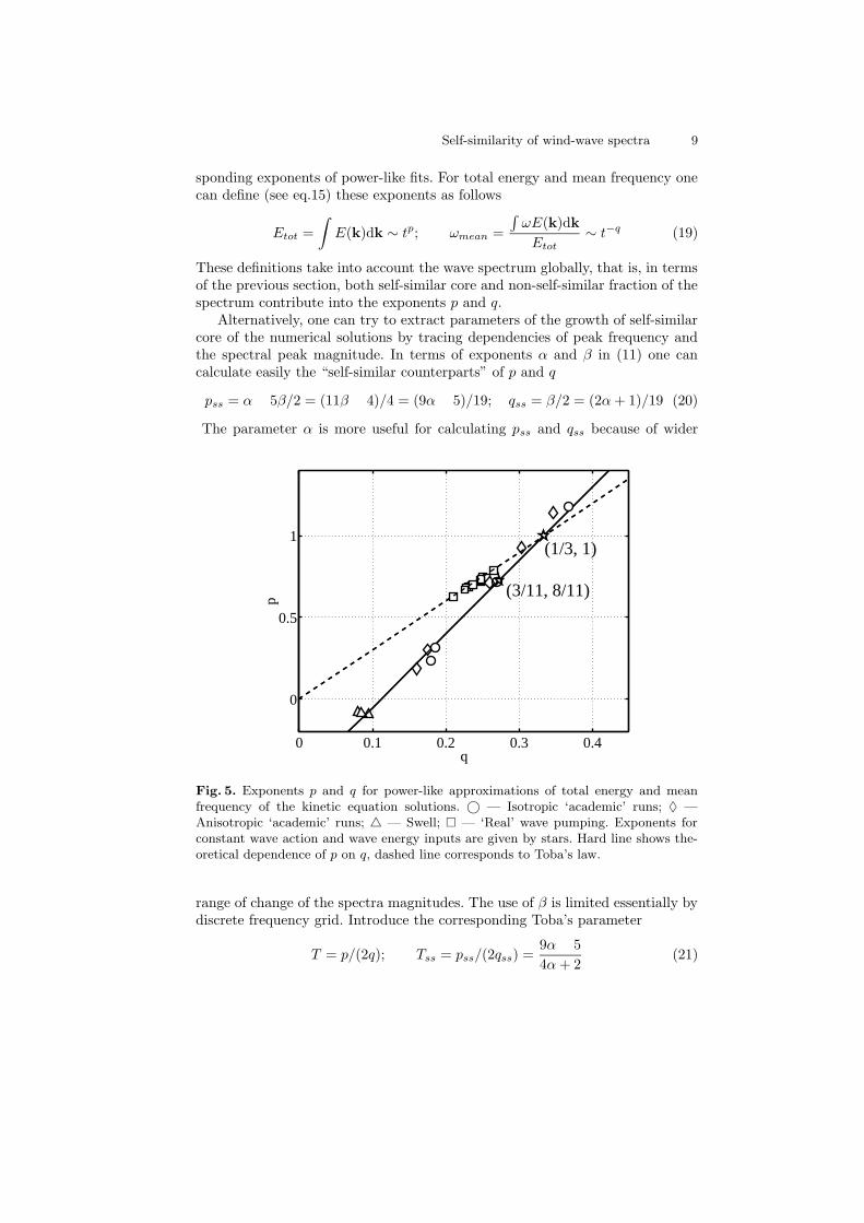
Self-similarity of wind-wave spectra 9
sponding exponents of power-like fits. For total energy and mean frequency one
can define (see eq.15) these exponents as follows
Etot =
∫
E(k)dk ∼ tp; ωmean =
∫
ωE(k)dk
Etot∼ t−q (19)
These definitions take into account the wave spectrum globally, that is, in terms
of the previous section, both self-similar core and non-self-similar fraction of the
spectrum contribute into the exponents p and q.Alternatively, one can try to extract parameters of the growth of self-similar
core of the numerical solutions by tracing dependencies of peak frequency and
the spectral peak magnitude. In terms of exponents α and β in (11) one can
calculate easily the “self-similar counterparts” of p and q
pss = α¡ 5β/2 = (11β ¡ 4)/4 = (9α¡ 5)/19; qss = β/2 = (2α + 1)/19 (20)
The parameter α is more useful for calculating pss and qss because of wider
0 0.1 0.2 0.3 0.4
0
0.5
1
p
q
(1/3, 1)
(3/11, 8/11)
Fig. 5. Exponents p and q for power-like approximations of total energy and meanfrequency of the kinetic equation solutions. © — Isotropic ‘academic’ runs; ♦ —Anisotropic ‘academic’ runs; 4 — Swell; ¤ — ‘Real’ wave pumping. Exponents forconstant wave action and wave energy inputs are given by stars. Hard line shows the-oretical dependence of p on q, dashed line corresponds to Toba’s law.
range of change of the spectra magnitudes. The use of β is limited essentially by
discrete frequency grid. Introduce the corresponding Toba’s parameter
T = p/(2q); Tss = pss/(2qss) =9α¡ 5
4α + 2(21)

10 Sergei Badulin et al.
0 0.1 0.2 0.3 0.4
0
0.5
1
p ss
qss
(1/3, 1)
(3/11, 8/11)
Fig. 6. The same as in previous figure for exponents pexp and qexp calculated for theparameters of solutions’ peaks (exponents α and β of the self-similar solutions).
that describes the power-like dependence of significant wave height on wave
period (frequency)
A ∼ (1/ω)T
The empirical value of the exponent T = 3/2 has been obtained by Toba [19].
Fig.5 presents values of exponents of wave growth for different numerical exper-
iments with both “academic” and “realistic” functions of wave input. One can
see that “academic” series follow the self-similar relation (20) rather than Toba’s
law 3/2. At the same time the “realistic” series give the exponents that are closer
to Toba’s exponent 3/2 (dashed line). This divergence in “academic” and “real-
istic” dependencies becomes vanishing if we consider the wave growth exponents
pss, qss for the self-similar core of wave spectra (fig.6). The peak frequency is
growing faster than the mean frequency while the energy of the self-similar core
is growing slower than the full wave energy, i.e. the non-self-similar fraction of
wind-wave field can affect essentially wave growth features.
5 Discussion. A Composite Model of Wind-Wave Balance
and Predictability of Wind-Wave Spectra
In this paper we showed that the self-similar solutions of the Hasselmann equa-
tion give a good approximation to the observed wind-wave spectra and parame-
ters of wind-wave growth. These approximate solutions do not take into account
details of wave input but depend on integral properties of this input. The asymp-
totic procedure that leads to these solutions implies a splitting of the wind-wave

Self-similarity of wind-wave spectra 11
balance into two parts. First, the “conservative” Hasselmann equation with no
generation or dissipation terms describes a family of spectral shapes
dNk
dt= Snl (22)
The parameters of the particular solution of the family is specified by the equa-
tion of integral balance of wave action (energy)
〈dNk
dt〉 = 〈Sin + Sdiss〉 (23)
In the consideration presented above these parameters are nothing but exponents
of temporal growth of total wave action (energy). It should be stressed that the
composite model is valid not for all waves but for those only which evolution is
governed predominantly by non-linear transfer. Strictly speaking, the model is
valid for a self-similar “core” of the solutions of the Hasselmann equation.
A key result of the present study is: the self-similar forms of wave spectra
given by (22) depend very slightly on the integral balance (23). Thus, the quasi-
universal spectra can be characterized effectively by their peak positions and
magnitudes. This note becomes very important for non-self-similar background
of wind-wave spectra. This background is beyond the composite model (22, 23).
It depends on details of wind-wave balance and can affect essentially the integral
energy and mean frequency. Thus, the prediction of the background behaviour
is less reliable than one of the self-similar core. At the same time, the mean
frequency and the total energy that characterize this background are easier to
be measured in the ocean than the spectral peak properties.
As it was pointed out in Introduction, occurrence of rogue waves is likely
associated with certain stages of wind-wave development. In our opinion, the
analysis of wind-wave state in terms of the concept of self-similarity presented
above can help in more adequate description of the wind-wave state in the con-
text of rogue wave dynamics.
The research was conducted under US Army Corps of Engineers grants
W912HZ-04-P-0172 and DACW42-03-C-0019, INTAS grant 01-234, ONR grant
N00014-03-1-0648, Russian Foundation for Basic Research 02-05-6514, 04-05-
64784 and the Russian Academy Program “Nonlinear Dynamics”. S.I. Badulin
acknowledges support of NATO under the linkage grant EST.CLG.978941.
References
1. Babanin, A.N. & Soloviev, Yu.P: Field investigation of transformation of the windwave frequency spectrum with fetch and the stage of development, Journ.Phys.Oceanogr. 28 (1998) 563–576
2. Badulin, S., Pushkarev, A., Resio, D., Zakharov, V.: Direct and inverse cascade ofenergy, momentum and wave action in wind-driven sea. 7th International workshopon wave hindcasting and forecasting. Banff, October 2002, (2002) 92–103

12 Sergei Badulin et al.
3. Badulin, S., Pushkarev, A., Resio, D., Zakharov, V.: Self-similarity of wind-drivensea. Submitted to J. Fluid Mech. (2005)
4. Battjes, J.A., Zitman, T.J. & Holthuijsen, L.H.: A reanalysis of the spectra observedin JONSWAP. J.Phys.Oceanogr. 17 (1987) 1288–1295
5. Donelan, M.A., Hamilton J., Hui W.H.: Directional spectra of wind-generatedwaves. Phil.Trans.Roy.Soc.Lond. A315 (1985) 509–562
6. Donelan, M.A. & Pierson-jr., W.J.: Radar scattering and equilibrium ranges inwind-generated waves with application to scatterometry, Journ.Geoph.Res. 92, C5(1987) 4971–5029.
7. Gunson, J., Holt, M.: Diagnostics for rogue wave development from spectral wavemodel hindcasts. Geophysical Research Abstracts 4 (2002) EGS02-A-05665
8. Hasselmann, K.: On the nonlinear energy transfer in a gravity wave spectrum. Part1, J.Fluid Mech. 12 (1962) 481-500
9. Hasselmann, K.: On the nonlinear energy transfer in a gravity wave spectrum. Parts2 and 3. J.Fluid Mech. 15 (1963) 273–281; 385-398
10. Hasselmann, K., Barnett, T.P., Bouws, E., Carlson, H., Cartwright, D.E., Enke, K.,Ewing, J.A., Gienapp, H., Hasselmann, D.E., Kruseman, P., Meerburg, A., Muller,P., Olbers, D.J., Richter, K.,Sell, W. & Walden, H.: Measurements of wind-wavegrowth and swell decay during the Joint North Sea Wave Project (JONSWAP),Dtsch.Hydrogh.Z.Suppl. 12 A8 (1973)
11. Hsiao, S.V. & Shemdin, O.H.: Measurements of wind velocity and pressure with awave follower during MARSEN. J.Geoph.Res. 88, C14 (1983) 9841–9849
12. Holt, M., Fullerton, G., Li, J.-G.: Forecasting sea state with a spectral wave model.Rogue Waves 2004 Brest, 20-22 October 2004
13. Osborne, A. R., Onorato, M. & Serio, M.: The nonlinear dynamics of rogue wavesand holes in deep water gravity wave trains. Phys. Lett. A 275 (2000) 386–393
14. Plant, W.J.: A relationship between wind stress and wave slope. Journ.Geoph. Res.87, C3, (1982) 1961–1967.
15. Pushkarev, A.N., Resio, D., Zakharov, V.E.: Weak turbulent theory of the wind-generated gravity sea waves. Physica D: Nonlinear Phenomena, 184 (2003) 29-63.
16. Resio, D. & Perrie, W.: A numerical study of nonlinear energy fluxes due to wave-wind interactions, J.Fluid.Mech. 223 (1991) 603–629
17. Snyder, R.L., Dobson, F.W., Elliot, J.A. & Long, R.B.: Array measurements ofatmospheric pressure fluctuations above surface gravity waves, J.Fluid.Mech. 102
(1981) 1–59.18. Stewart, R.W.: The air-sea momentum exchange, Boundary-Layer Meteorology 6
(1974) 151–167.19. Toba, Y.: Local balance in the air-sea boundary processes. III. On the spectrum
of wind waves, J.Oceanogr.Soc.Japan 29 (1973) 209–220.20. Webb, D.J.: Non-linear transfers between sea waves. Deep-Sea Research 25 (1978)
279–29821. Young, I.R.: Wind Generated Ocean Waves. Elsevier (1999)22. Zakharov, V.E. & Filonenko N.N.: Energy spectrum for stochastic oscillations of
the surface of a fluid, Dokl.Acad.Nauk SSSR 160 (1966) 1292–129523. Zakharov, V.E., Zaslavsky M.M.: The kinetic equation and Kolmogorov spectra in
the weak-turbulence theory of wind waves, Izv.Atm.Ocean.Phys., 18 (1982) 747–753.
24. Zakharov, V.E.: Theoretical interpretation of fetch limited wind-driven sea obser-vations. 7th International workshop on wave hindcasting and forecasting, Banff,October 2002, (2002) 86–92

Spatial Extremes, Shapes of Large Waves, and
Lagrangian Models
Herve Socquet–Juglard and Kristian B. Dysthe, University of Bergen,
Karsten Trulsen, University of Oslo,
Sebastien Fouques, Jingdong Liu, and Harald E. Krogstad1), NTNU,
Trondheim
1) NTNU, Trondheim, [email protected]
Abstract. The paper rst states a simplied formulation of V. I. Piter-barg’s theorem about extremes of Gaussian elds, which together withthe Slepian Model Representation is a general tool for analyzing thespatial characteristics of ocean waves. We then consider numerical simu-lations of random surface gravity waves carried out in space and time bymeans of modied nonlinear Schrodinger equations. It is demonstratedthat high waves in the simulations are steeper and more asymmetricthan predicted by the Gaussian theory. The last part of the paper dis-cusses Lagrangian stochastic models as alternatives to the conventionalEulerian rst and second order models.
Introduction
Today we are starting to obtain spatial measurements of ocean waves by remote
sensing techniques (Schulz-Stellen eth and Lehner, 2004), and questions about
spatial and even spatio/temporal extremes arise. For rogue waves the question
naturally comes up whether such waves are truly exceptional, or whether they
may actually happen somewhere or sometimes in a storm sea with considerable
temporal and spatial extent.
Spatial data need tools from spatial statistics. The Slepian Model Repre-
sentation (SMR) for Gaussian elds is well known [8]. In ocean engineering it
forms the basis for New Wave Theory [17], the analysis of the shapes of extreme
Gaussian waves [11], and the Boccotti theory of Quasi Determinism [1]. Another
result of more recent origin is an explicit expression for the asymptotic extreme
value distribution of a Gaussian eld of arbitrary dimension derived by V. I.
Piterbarg [14]. A simplied formulation of the theorem is given below.
The tools have been applied for analysis of spatial numerical simulations of
random surface gravity waves of moderately narrow spectral bandwidth. The
simulations utilize the Modied Nonlinear Schrodinger equations and produce
the time development of sections of the ocean surface of the order 100 × 100
typical wavelengths and over 150 wave periods [18], [19]. Below we show a few
results about the shape of the individual high waves. An extended discussion
about extreme value distributions has been given elsewhere [16].

The nal part reports from ongoing work investigating three dimensional
second order Lagrangian stochastic models of the surface. Already at the rst
order, stochastic Lagrangian waves deviate signicantly from linear Eulerian
waves, and second order theory shows new and interesting features.
1 Gaussian Fields
Consider a zero mean homogeneous Gaussian eld, X (x) , x ∈ Rn, with covari-
ance function ρ (x), ρ (0) = 2, and spectrum Ψ (k),
ρ (x) =
∫
k
eikxΨ (k) dk. (1)
We shall assume that the covariance matrix, Λ, of ∇X = ∂X/∂xini=1 is non-
singular. The covariance matrix may be expressed as
Λ =
∫
k
kk′Ψ (k) dk. (2)
By turning to the principal axis, Λ becomes diagonal and denes intrinsic spa-
tial scales of the eld, ξk = 2/ν1/2k , k = 1, · · · , N , where νk is the k-th eigen-
value of Λ/2. The scales dene a unit cell with volume |V | = ξ1 × · · · × ξn =
(2)n ∣
∣Λ/2∣
∣
1/2. When n = 1 and x is time, the length of the unit cell is equal
to the mean zero-upcrossing period, Tz. For n = 2 and x = (x1, x2), the scales
are the mean wavelength, λ0, and the mean crest length, λc, and |V | = λ0λc.
For the space-time case, (x, t), an additional correction term due to the space-
time correlation is needed, |V | = λ0λcTz
(
1 − C20t − C2
ct
)
1/2. Here C0t is the
correlation between ∂X/∂x0 (0, 0) and ∂X/∂t (0, 0), and similarly for Cct.
The Slepian Model Representation (SMR) follows from the general theory of
multivariate Gaussian variables, where conditional expectations and prediction
errors are expressed in terms of the covariance functions. We shall only use the
result for the behavior around a high maximum at x = 0, where ∇X = 0:
Xs (x) = X (x) |X (0) = a,∇X (0) = 0 = aρ (x)
ρ (0)+ ∆ (x) . (3)
The residual process ∆ (x) is Gaussian with E (∆ (x)) = 0, and
Var (∆ (x)) = ρ (0) −ρ (x)
2
ρ (0)−∇ρ (x) Λ1 (∇ρ (x))
′ . (4)
The approximation Xs (x) v a ρ(x)ρ(0) is only reasonable when ∆ (x) is small. In the
present case this is at most for the extension of the unit cell centered at x = 0,
beyond which Var∆(x) → 2.
Piterbarg’s Theorem ([14], Theorem 14.1) considers homogeneous Gaussian
elds in Rn and the asymptotic extreme value distributions for the maximum
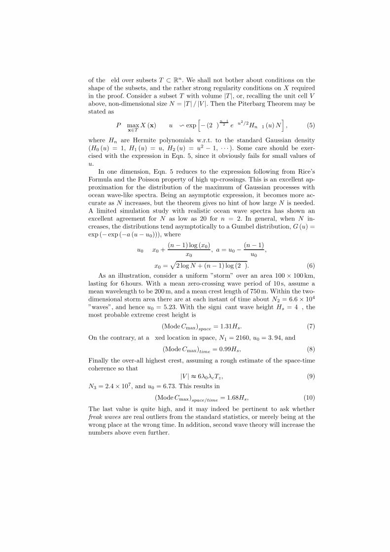
of the eld over subsets T ⊂ Rn. We shall not bother about conditions on the
shape of the subsets, and the rather strong regularity conditions on X required
in the proof. Consider a subset T with volume |T |, or, recalling the unit cell Vabove, non-dimensional size N = |T | / |V |. Then the Piterbarg Theorem may be
stated as
P
maxx∈T
X (x) u
v exp[
− (2)n1
2 eu2/2Hn1 (u) N]
, (5)
where Hn are Hermite polynomials w.r.t. to the standard Gaussian density
(H0 (u) = 1, H1 (u) = u, H2 (u) = u2 − 1, · · · ). Some care should be exer-
cised with the expression in Eqn. 5, since it obviously fails for small values of
u.
In one dimension, Eqn. 5 reduces to the expression following from Rice’s
Formula and the Poisson property of high up-crossings. This is an excellent ap-
proximation for the distribution of the maximum of Gaussian processes with
ocean wave-like spectra. Being an asymptotic expression, it becomes more ac-
curate as N increases, but the theorem gives no hint of how large N is needed.
A limited simulation study with realistic ocean wave spectra has shown an
excellent agreement for N as low as 20 for n = 2. In general, when N in-
creases, the distributions tend asymptotically to a Gumbel distribution, G (u) =
exp (− exp (−a (u − u0))), where
u0 x0 +(n − 1) log (x0)
x0, a = u0 −
(n − 1)
u0,
x0 =√
2 log N + (n − 1) log (2). (6)
As an illustration, consider a uniform ”storm” over an area 100 × 100 km,
lasting for 6 hours. With a mean zero-crossing wave period of 10 s, assume a
mean wavelength to be 200m, and a mean crest length of 750m. Within the two-
dimensional storm area there are at each instant of time about N2 = 6.6 × 10⁴
”waves”, and hence u0 = 5.23. With the signicant wave height Hs = 4, the
most probable extreme crest height is
(Mode Cmax)space = 1.31Hs. (7)
On the contrary, at a xed location in space, N1 = 2160, u0 = 3. 94, and
(Mode Cmax)time = 0.99Hs, (8)
Finally the over-all highest crest, assuming a rough estimate of the space-time
coherence so that
|V | ≈ 6λ0λcTz, (9)
N3 = 2.4× 10⁷, and u0 = 6.73. This results in
(Mode Cmax)space/time = 1.68Hs, (10)
The last value is quite high, and it may indeed be pertinent to ask whether
freak waves are real outliers from the standard statistics, or merely being at the
wrong place at the wrong time. In addition, second wave theory will increase the
numbers above even further.

Numerical Simulations
We refer to [3] for a discussion about the numerical simulation model based on the
Modied Non-Linear Schrodinger(MNLS) equation. The numerical simulations
shown below are all based on the evolution of a stochastic wave eld with initial
wave spectra based on the JONSWAP form and a cos- directional distribution,
E (ω, θ) = S (ω) D (θ) ,
S (ω) =
ω5 exp
[
−5
4
ω
ωp
4]
exp((ω/ωp1)2/2σ2J), (11)
D(θ) =
1 cos2(
πθ2
)
, |θ| < ,
0, |θ| .(12)
The corresponding wavenumber spectrum, truncated for |k − k0| > k0, is used
for the initialization of the Fourier amplitudes. In all simulations, kp = 1, and
J and have the standard average JONSWAP-values. The spectrum is scaled
with to an overall steepness s = Hs/λp = 0.045, typical for real ocean waves
of some size. Only two dierent cases are shown below. For Case A, = 0.7,
corresponding to a directional spread 1 = 14, and for Case B, = 0.35,
corresponding to 1 = 7.2.The simulated domain is square with sides 128×λp, and the simulations cover
a time span of 150 × (2/ωp). During this time period the spectrum changes
slowly, and this has some impact on the mean wave and crest lengths of the
elds.
The SMR gives a stochastic description of the spatial shape of high maxima
for Gaussian processes. The upper pair of plots in Fig. 1 shows a color-coded
graph of the surface, reconstructed to 3rd order, around the maximum along with
the SMR prediction for a Gaussian eld with the same covariance function. We
observe that the simulation shows a denitely narrower crest in the wave propa-
gation direction, whereas the crest length is comparable to the SMR prediction.
The SMR prediction drops to 0 quite fast away from the maximum and the
prediction error, ∆ (x) , takes over. This is illustrated in the lower plots, where
we show cuts through the maximum crest along the wave propagation direction
and in the orthogonal direction to that, the wave crest direction. Plus/minus 2
standard deviations of ∆ (x) are shown along with the actual outcome of the
simulation on top, and we observe that the SMR prediction quickly becomes of
limited value away from the peak.
In order to draw more rm conclusions about the shape of the surface around
the crest, it is therefore necessary to average the simulations over several maxima
and compare the mean to the SMR prediction. This is, however, somewhat tricky
since the spectrum and hence the covariance function and the SMR vary over the
time span of the simulations. An example using Case A, which undergoes only a
minor spectral changes, is shown in Fig. 2. It is obvious that the average crest
from the simulations is narrower than the SMR prediction, and the extension
of the surrounding troughs is larger. When inspecting individual realizations, as

Fig. 1. Excerpt around the maximum peak of a simulation for Case A after 150Tp.Top left: Color-coded surface elevation. Top right: SMR prediction. Bottom left: Cutthrough the maximum in the wave propagation direction. Black: Actual prole. Red:SMR prediction ±2 std ∆ (x). Bottom right: Cut in the orthogonal (crest) direction.
shown in Fig. 1, it is often seen that the crests are longer than predicted by
SMR, but bent in various directions. On the average, the crest length in the
direction orthogonal to the main propagation direction is similar to the SMR.
Figure 3 demonstrates this for cuts in the wave and orthogonal crest directions
for both Case A and B. Along the wave propagation direction, the waves are
steeper than predicted by the SMR. Moreover, as a consequence of the second
order contribution, the troughs on each side are signicantly shallower than
linear wave theory predicts. The wave as a whole is therefore more vertically
asymmetric. The average dierence in crest lengths is minor, but this is an
average in the orthogonal direction to the wave propagation, and not the length
of the actual crests, which, as noted above, tend to be bent.
2 Lagrangian Models
The traditional ocean surface wave theory is based on a perturbation expansion
of the Eulerian equations of motion for an incompressible and inviscid uid. This
approach has been applied successfully to model gross features of the waves as
long as their overall steepness remains small. However, issues such as the esti-
mation of radar backscatter from the sea surface depend strongly on the slope
and curvature of the ocean surface on many scales. This requires a description
of the waves which is rather difficult to achieve through the Eulerian approach.

Fig. 2. Average surface shape around the maxima for Case A (left) compared to theSMR prediction, also averaged over the time span of the simulations (right).
A A
B B
h h
h h
Fig. 3. Average cuts in the wave and crest directions for Case A (upper) and Case B(lower) . Solid: simulations, dashed: SMR prediction.

Recently, the interest for a Lagrangian description of ocean gravity waves has
increased ([10], [2], [9], [5]). In this approach [6], one considers the motion of in-
dividual uid particles, and the free surface is derived from the surface particles’
positions [7]. As a result, the surface elevation is described through a paramet-
ric representation, which allows a larger exibility as far as the wave shape is
concerned.
In the Lagrangian model, the uid is described through a set of uid particles
located at X = (x, y, z)T at a given time t. The coordinate system has origin
at the mean water level with z pointing upwards. Each particle is labelled by
its reference position X0 = (, , δ)T . The uid is assumed to be incompressible
and inviscid, and the ow irrotational. The conservation of momentum can then
be integrated to
∇L × (JXt) = 0, (13)
and the mass conservation reads [7]
det(J) = 1, (14)
where J ≡ ∇TL X
T , ∇L ≡ (∂/∂∂/∂ ∂/∂δ). The boundary conditions are
δ = 0 at the surface
p = 0 for δ = 0
zt → 0 for δ → −∞.(15)
A perturbation expansion of equations (13)–(15) has been carried out in [12]
and [13]. According to dimensional analysis, the small parameter ε is proportional
to ||J − 1||, where ‖‖ is any matrix norm of R3×3. Thus, ε is related to the
Lagrangian gradient of the distance between the particles and their reference
positions X0. This diers from the Eulerian approach, where the small parameter
of the perturbation expansion is the wave slope. The displacement of the particles
is now written as X = X0 + X1 + X2 + · · · , where Xn = O (εn).
The rst order solution is similar to the irregular extension of the Gerstner
wave [4] given by Pierson (1961).
x1 = −∑
p
kp
kpape
kpδ sinΨp (16)
z1 =∑
p
apekpd cosΨp (17)
with Ψp = kpx0 −pt+φp, and where kp = |kp| and 2p = gkp. The wave proles
show sharper crests and broader troughs. It is also capable of capturing some
non-resonant wave-wave interactions such as the modulation of the crest-to-crest
distance of short waves riding on the top of longer ones, as depicted in Fig. 4.
Besides, it can be shown that the interaction of two rst order wave compo-
nents with similar frequencies brings about a second order non-uniform current,
whose main eect is to bend short crested waves. These so-called horseshoe
patterns have also been observed to form in simulations based on the MNLS

0 10 20 30 40 50 60 70 80−2
−1.5
−1
−0.5
0
0.5
1
1.5
2
x [m]
z [m]
Fig. 4. First order bi-chromatic Lagrangian waves.
y [m
]
t=0s
-250 -200 -150 -100 -50 0
-50
0
50
y [m
]
t=7.1581s
-250 -200 -150 -100 -50 0
-50
0
50
x [m]
y [m
]
t=14.3163s
-250 -200 -150 -100 -50 0
-50
0
50
Fig. 5. Second order irregular Lagrangian waves in three dimensions developing ”horse-shoe patterns”.

−10 −5 0 5 10 15 20 25 30 35−5
0
5
t=1
.5s
−10 −5 0 5 10 15 20 25 30 35−5
0
5
t=2
s
−10 −5 0 5 10 15 20 25 30 35−5
0
5
t=2
.5s
−10 −5 0 5 10 15 20 25 30 35−5
0
5
t=3
s
−10 −5 0 5 10 15 20 25 30 35−5
0
5
x [m]
t=3
.5s
Fig. 6. Second order irregular Lagrangian waves (solid lines). Corresponding rst orderLagrangian surface (dash-dotted line). The grid is regular in the reference coordinates.
equation [20], but are already seen at second order in the Lagrangian approach
(see Fig. 5). The well-known Stokes drift is obtained from the second order
interaction of a rst order wave component with itself. Besides, for irregular
waves, large horizontal displacement waves at the second order are responsible
for asymmetric wave proles with steep fronts, as shown in Fig. 6.
However, the second order mass transport induces an increase in the horizon-
tal displacement of the uid particles. Consequently, the small parameter of the
perturbation expansion also grows towards innity, and the duration of validity
of the model is limited.
Conclusions
The Slepian Model Representation and Piterbarg’s asymptotic extreme value
distribution represent valuable tools for analyzing spatial elds. Piterbarg’s The-
orem gives a simple expression for the extreme values in Gaussian elds in any
dimension, and may, in particular, answer questions about the maximum crest
height in an area at a xed time, or the overall highest crest in a spatially
extended eld lasting for some time.

The numerical simulations using the modied nonlinear Schrodinger equa-
tions give snapshots of the surfaces over a typical area 128×128 wavelengths and
at time instances ranging from 0 to 150Tp. During this time span, the simulated
wave elds undergo some spectral change, as discussed in [3]. The simulated
surfaces have been reconstructed to rst, second and third order, and for the
shape of the highest waves, the simulations show systematically steeper waves
in the wave propagation direction and somewhat longer crests than the Gaus-
sian prediction obtained from the SMR. Individual realizations often show that
the crests bend. Simulated high waves are therefore signicantly more vertically
asymmetric than the corresponding Gaussian waves.
The Lagrangian stochastic models represent interesting alternatives to the
conventional Eulerian models. Already at the rst order, stochastic Lagrangian
waves deviate signicantly from linear Eulerian waves, and second order theory
develops new and interesting features.
Acknowledgments
This research has been supported by the BeMatA programme of the Research
Council of Norway (139177/431) and NTNU University Grant No. 70080000.
References
1. Boccotti, P. (2000), Wave Mechanics for Ocean Engineering, Elsevier, Amsterdam.2. Chang, M.-S. (1969), Long-crested random graviy waves, J. Geophys. Res., 74(6),
1515–1536.3. Dysthe, K. B., K. Trulsen, H. E. Krogstad, and H. Socquet-Juglard (2003), Evolu-
tion of a narrow band spectrum of random surface gravity waves, J. Fluid Mech.,
478, 1–10.4. Gerstner, F. J. (1809), Theorie der Wellen. Gilbert’s Annalen der Physik., xxxii.5. Gjøsund, S. H. (2003), A Lagrangian model for irregular waves and wave kinemat-
ics. Trans. of the ASME, Journal of Offshore Mechanics and Arctic Engineering,
125, 94–102.6. Lagrange, J. L. (1788), Mecanique Analytique, Jacques Gabay, Paris. Reprint 1989.7. Lamb, H. (1932), Hydrodynamics, Cambridge University Press, 6th edition.8. Lindgren, G. (1972), Local maxima of Gaussian Fields, Arkiv for Matematik, 10,
195–218.9. Moe, G., Ø. A. Arntsen, and S. H. Gjøsund (1998), Wave kinematics based on a
Lagrangian formulation. Proc. of the 1998 International OTRC Symposium ”Ocean
Wave Kinematics, Dynamics and Loads on Structures”, ASCE Press, 56–63.10. Phole, F. V. (1950), The Lagrangian equations of hydrodynamics: solutions which
are analytic functions of the time,0 Ph.D. Thesis, Graduate School of Arts andScience, New York University.
11. Phillips, O. M., D. Gu, and E. J. Walch (1993), On the Expected Structure ofExtreme Waves in a Gaussian Sea. Part II: SWADE Scanning Radar AltimeterMeasurements, J. Phys. Ocean., 23, 2297–2309.
12. Pierson, W. J. (1961), Models of random seas based on the Lagrangian equationsof motion, Tech. Rept. Contr. Nonr-285(03). College of Engineering, ResearchDivision, New York University.

13. Pierson, W. J. (1962), Perturbation analysis of the Navier-Stokes equations in theLagrangian form with selected linear solutions, J. Geophys. Res., 67(8), 3151–3160.
14. Piterbarg, V. I. (1996), Asymptotic Methods in the Theory of Gaussian Processes
and Fields, AMS Transl. of Math. Monographs, 148, Providence, R.I.15. Schulz-Stellen eth, J. and S. Lehner (2004), Measurement of two dimensional sea
surface elevation elds from complex synthetic aperture radar data, IEEE Trans.
Geos. Rem. Sensing, 42(6), 1149 – 1160.16. Socquet-Juglard, H., K. B. Dysthe, K. Trulsen, H. E. Krogstad, and J. Liu (2004),
Probability distributions of surface gravity waves during spectral changes, submit-ted to J. Fluid Mech.
17. Tromans, P. S., A. R. Anaturk, and P.M. Hagemeijer (1991), A new model for thekinematics of large ocean waves – applications as a design wave, in Proc. 1st Int.Oshore and Polar Engng. Conf., Edinburgh, UK, 3, 54–71.
18. Trulsen, K. and K. B. Dysthe (1996), A modied nonlinear Schrodinger equationfor broader bandwidth gravity waves on deep water, Wave Motion, 24, 281–289.
19. Trulsen, K., I. Kliakhandler, K. B. Dysthe, and M. G. Velarde (2000), On weaklynonlinear modulation of waves on deep water, Phys. Fluids, 2, pp. 2432–2437.
20. Trulsen, K. (2004), Large horseshoe patterns of water surface waves, submitted J.
Fluid Mech.

Wave crest statistics calculated using a fullynonlinear spectral response surface method
Richard Gibson‡, Chris Swan‡, Peter Tromans†‡ & Luc Vanderschuren†
‡ Department of Civil and Environmental EngineeringImperial College London
SW7 2AZUnited Kingdom
† Ocean Wave Engineering LtdLiss
HampshireGU33 7AT
United [email protected], [email protected] [email protected],
Abstract. This paper is concerned with the calculation of the proba-bility of exceedence of wave crest elevation. This has important implica-tions for the design of both fixed and floating structures. In particular,the paper is interested in identifying sea-states in which so-called freak,or rogue, waves are intrinsically more likely to occur. This is investigatedby ascertaining the effect that both the bandwidth and the directionalspread of a spectrum has on the statistics of crest elevation. By com-bining a fully-nonlinear numerical wave-model with a spectral responsesurface method, statistics that include the full-nonlinearity of the wave-field can be determined very efficiently. It has been shown that whilst inunidirectional sea-states linear and second-order theory underestimatesthe probability of exceedence of crest elevation, this is not the case inmost directionally spread wave-fields. Furthermore, by combining theshort-term statistics relevant to sea-states with the long-term statisticsof storms, the return period of the Draupner New Year’s wave has beenestimated.
1 Introduction
A knowledge of the statistics of wave crest elevation is fundamental for the designof most marine structures. For example, the occurrence of the largest wavesdetermines the required air-gap and the maximum drag force on a fixed structure.Furthermore, it is important in the estimation of green-water inundation and theincidence of wave slam on floating structures. However, it has been suggested thatsome of the largest waves occur more often than would be predicted by linear, orsecond-order, theory. These waves are often referred to as freak, or rogue, waves.In this paper the short-term statistics of wave crest elevation are calculated byincorporating the fully nonlinear numerical wave-model of Bateman et al. (2001)

into a spectral response surface (SRS) method. The results of the short-termstatistics have then been incorporated into the long-term statistical method ofTromans & Vanderschuren (1995) and the return period of a particular crestelevation at a particular location can be calculated. This method has been usedto analyze hindcast data at the Draupner location and the return period ofthe January 1 1995 Draupner wave has been calculated. The paper begins in§2 by describing the theoretical basis and application of the SRS method. Itcontinues in §3 by applying the method to calculate the short-term statistics ofcrest elevation in both unidirectional and directional sea-states. In §4 the SRSmethod is incorporated into that of Tromans & Vanderschuren (1995) and thereturn period of the Draupner wave is calculated. Concluding remarks can befound in §5.
2 SRS Method
The SRS method has been used in structural engineering to calculate the prob-ability that a structure will fail when subjected to a number of statisticallyindependent loads.
In this paper the SRS method is applied in order to calculate the probabilityof exceedence of crest elevation. A brief description of how this is undertakenfollows; a more detailed description can be found in Gibson et al. (2005). The SRSmethod is applied by discretising the spectrum into a number of independentcomponents, the statistical distribution of which is given by their variance, σ2
n.The components are directly related to the surface elevation, and therefore, inorder to consider their phasing, must be divided into ηn:
ηn = an cos(ωnt− ϕn) , (1)
and its Hilbert transform, ηn:
ηn = an sin(ωnt− ϕn) , (2)
where an is the amplitude of the nth component, ωn its frequency and ϕn its ran-dom phase angle. These components are then standardised, by subtracting theirmean and dividing by their standard deviation, σn. Figure 1 shows a surface, inthis case a circle, of constant probability density in the space of the standardisedvariables xn and xn. The point A represents one particular event, its responseis R(xn, xn), and its probability density is directly related to its distance fromthe origin, β =
√x2
n + x2n. A first order reliability method (FORM) can then be
applied in order to estimate its probability of exceedence, this is given as:
Q = P (Crest elevation > R(x, x)) = exp(−β(x, x)2
2
). (3)
Therefore, each circle, or in more than two-dimensions each ‘hyper-sphere’, rep-resents one probability of exceedence. A standard optimisation routine, such asthat of Fletcher-Reeves (Press et al., 1994), is then applied in order to find the

maximum value of the response that corresponds to a particular probability ofexceedence. In this case the response is crest elevation, which according to lineartheory is given by
R(xn) =N∑
n=1
(σnxn) . (4)
However, the technique can be used for other responses, such as that of a struc-ture subject to wave loading.
−2 −1 0 1 2−2
−1.5
−1
−0.5
0
0.5
1
1.5
2
Standardised wave component x1
Sta
ndar
dise
d w
ave
com
pone
nt x
2
Response Surface
b
c β
A
Fig. 1: A surface of constant probability density. The event A corresponds tox1 = b and x2 = c and has a probability density that is directly related to β.
3 Short-term statistics
The SRS method has been applied in order to calculate the probability of excee-dence of crest elevation in both unidirectional and directional sea-states. Thishas been achieved using a first-order response function described in equation4, a second-order response function based upon Sharma & Dean (1981) anddescribed in Tromans & Vanderschuren (2002), and a fully-nonlinear responsefunction obtained by incorporating the fully-nonlinear wave-model of Batemanet al. (2001) into the SRS method. The fully-nonlinear response function hasbeen generated two ways. The first is by using the spectrum optimised linearlyas the input to the wave-model and obtaining a fully-nonlinear correction tothe crest elevation. This is an underestimate of the actual crest elevation as the

spectrum has not been optimised fully-nonlinearly. The second method addressesthis short-coming and optimises the spectrum fully-nonlinearly. Unfortunately,this is an extremely time-consuming process as the wave model, whilst efficient,must be run many times for each wave component for each probability of excee-dence. Accordingly, only a few probabilities of exceedence have been optimisedfully-nonlinearly in the unidirectional sea-states, and only one in the directionalsea-states.
3.1 Unidirectional Seas
The SRS method has been applied to two unidirectional spectra, J1D0 andJ5D0. Both are JONSWAP spectra with peak period Tp = 12.8s; the formerhas a peak enhancement factor γ = 1.0, the latter a peak enhancement factorγ = 5.0. Figure 2 shows that the fully-nonlinear results give a substantial increasein crest elevation over the linear or second-order results. This is the result of therapid evolution of the wave spectrum discussed in more detail in Gibson & Swan(2004) and Gibson & Swan (2005). Furthermore, the figure also shows that themore narrow-banded spectrum, J5D0, is more nonlinear than J1D0, and thatit is only for this spectrum that a fully-nonlinear optimisation is required. Theincrease in nonlinearity with reduced bandwidth is confirmed in figure 3; thisindicates that the fully-nonlinear optimisation of both J1D0 and J5D0 selects aspectrum that is more narrow-banded. Further discussion and an investigationof the physical mechanisms that are responsible for these results can be foundin Gibson et al. (2005).
10−2
10−1
100
0
5
10
15
Probability of Exceedence (Q)
Max
imum
cre
st e
leva
tion
(m)
LinearSecond−order case J5D0Fully nonlinear case J1D0 approximate Fully nonlinear case J5D0 approximateFully nonlinear case J1D0 exactFully nonlinear case J5D0 exact
Fig. 2: The probability of exceedence of crest elevation in unidirectional seas.

0.01 0.02 0.03 0.04 0.05 0.06 0.07 0.080
0.5
1
1.5
Wave Number (rad m−1)
Am
plitu
de (
m)
Case J1D0 originalCase J1D0 optimisedCase J5D0 originalCase J5D0 optimised
Fig. 3: The original and optimised spectra for cases G1D0 and G5D0. The spectraare coarsely discretised due to the time consuming nature of the optimisationprocess.
3.2 Multi-directional Seas
The SRS method has also been applied to two directional spectra, J5D10 andJ5D30. Once again both are JONSWAP spectra with peak period Tp = 12.8sand peak enhancement factor γ = 5.0; in the former the standard deviation ofthe wrapped normal directional spreading function is σθ = 10, in the latter it isσθ = 30. Figure 4 indicates that for both spectra the fully-nonlinear crest ele-vation is less than the second-order prediction. Furthermore, the fully-nonlinearoptimisation of the wave spectra only marginally increases the crest elevation.This suggests that the focussing of wave components is not a mechanism bywhich rogue waves can form in sea-states characterised by a directionally spreadJONSWAP spectrum. This is the result of the balance between the spectral evo-lution, involving changes in both the frequency and the directional spectrum,and the focussing of the wave components discussed in more detail in Gibson &Swan (2004) and Gibson & Swan (2005).
Figure 5 shows the probability of exceedence of crest elevation for a direc-tionally spread Gaussian spectrum of Tp = 16s and σ = 5, characteristic ofswell-dominated sea-states. In this case the crest elevations are very much largerthan those of the JONSWAP spectrum. However, figure 5 also shows that inmixed sea-states, those in which there is both a wind (JONSWAP) and a swell(Gaussian) component, the result is similar to that for a purely wind-dominated(JONSWAP) sea.

10−3
10−2
10−1
100
2
4
6
8
10
12
Probability of Exceedence
Max
imum
Cre
st E
leva
tion
(m)
LinearSecond−orderFully nonlinear case J5D10 approximateFully nonlinear case J5D30 approximateFully nonlinear case J5D10 exactFully nonlinear case J5D30 exact
Fig. 4: The probability of exceedence of crest elevation in directional seas.
10−6
10−5
10−4
10−3
10−2
10−1
100
0
2
4
6
8
10
12
14
16
18
Probability of Exceedence (Q)
Cre
st E
leva
tion
(m)
LinearJONSWAP onlyGaussian onlyMixed Sea−state
Fig. 5: The probability of exceedence of crest elevation in wind dominated, swelldominated and mixed directional-spread sea-states. In the case of the mixed seathe amplitude has been split evenly between the wind and swell components.

4 Long-term statistics
The results of the previous section relate to the short-term statistics of sea-states.However, the design of a marine structure typically requires knowledge of thelong-term statistics at a particular location. This can be undertaken by applyingTromans & Vanderschuren (1995). The method considers storms as independentevents and requires two types of distribution to be defined. The first is the long-term statistics of storms, which is calculated from measured or hindcast data.The second is the short-term statistics of waves within a sea-state, which can becalculated using the SRS method. Tromans & Vanderschuren (1995) has beenapplied, in conjunction with the SRS method and using hindcast data for theDraupner location, in order to calculate the return period of an 18.5m crestelevation; corresponding to the New Year Wave recorded on January 1 1995.The manner in which this has been undertaken is described below.
If the spectrum is assumed to be JONSWAP then it is possible to constructa transfer function from linear to nonlinear crest elevation:
Cnl = Clin.F (ClinKp) , (5)
where Clin is the linear crest elevation, with a probability of exceedence definedby the Rayleigh distribution, Cnl is the nonlinear crest elevation and Kp is thewave-number of the peak of the spectrum. This ignores the parameters of thespectrum as previous results (Gibson & Swan, 2005) have indicated that, indirectional seas, they have little effect on the distribution of crest elevation. Theform of the transfer function, for a JONSWAP spectrum, is as follows:
F (ClinKp) = 1 + β(ClinKp)p + γ(ClinKp)q , (6)
where p and q are approximately one and two respectively. Using these values,the β term corresponds to the second-order bound correction, whilst the γ termcorresponds to the third-order resonant change to the amplitude of the under-lying linear spectrum. The various coefficients are given in table 1 and the fit tothe data described in figure 6.
Parameter Second-Order Fully-Nonlinearβ 0.50 0.87γ 0.0 -1.63p 1 1.17q 2 1.92
Table 1: Parameters of the transfer functions from linear to nonlinear crest ele-vation using Equations 6
Tromans & Vanderschuren (1995) can now be applied using linear theory witha nonlinear transfer function utilised at each step. Figure 7 depicts the return

period of crest elevation at the Draupner location calculated using linear, second-order and fully-nonlinear theory. This shows that the best estimate for the returnperiod of the New Year wave recorded at the Draupner platform wave is 800years; which is greater than the 300 years calculated using a second-order model.
5 Concluding Remarks
In this paper both short- and long-term statistics of crest elevation have beenconsidered. This has been undertaken by incorporating the fully-nonlinear wave-model of Bateman et al. (2001) into both the SRS method and that of Tromans &Vanderschuren (1995). The results have shown that whilst in unidirectional sea-states the fully-nonlinear crest elevations are significantly larger than those calcu-lated to second-order, this is not necessarily the case in directional seas. Indeed,in broad-banded directionally spread seas, characterised by a JONSWAP spec-trum, the fully-nonlinear crest elevations are in fact lower than those predicted tosecond-order. However, in narrow-banded swell-dominated seas, characterised bya Gaussian spectrum with a small spreading parameter, the results are similar tothose of the unidirectional simulations; with crest elevations significantly higherthan second-order theory. This suggests that it is in swell-dominated sea-statesthat rogue waves are intrinsically more likely to occur.
The SRS method has been used in conjunction with that of Tromans & Van-derschuren (1995) in order to calculate the return period of the Draupner wave.This has been undertaken by employing a transfer function from the linear tothe fully-nonlinear results. The result gives a return period of a 18.5m crest el-evation of 800 years.
Acknowledgement
The early stages of this work were undertaken within the project ‘ReliabilityBased Structural Design of FPSO Systems’, which involves Shell International,Instituto Superior Tcnico, DHI, Det Norske Veritas, Imperial College, NobleDenton and Oxford University. The project is partially funded by the EuropeanUnion through the Energy Programme under contract ENK6-2000-00107. Thelater stages of the work were completed with support from the UK Engineeringand Physical Sciences Research Council under grant number GR/R64971.

0 2 4 6 8 10 121
1.05
1.1
Linear Crest Elevation Clin
Rat
io o
f Cnl
/ C
lin
Second−order resultsSecond−order fitFully−nonlinear resultsFully−nonlienar fit
Fig. 6: The fit to the nonlinear crest elevations. In terms of Clin, the fittingfunction is parabolic for second-order results and cubic for the fully nonlinearresults; the latter indicating the dominance of third-order terms.
102
103
104
14
15
16
17
18
19
20
21
22
23
Return Period (years)
Cre
st E
leva
tion
(m)
LinearSecond−orderFully−nonlinear
Fig. 7: The return period of crest elevation at the Draupner location.

Bibliography
Bateman, W. J. D., Swan, C. & Taylor, P. H. 2001 On the efficient numer-ical simulation of directionally-spread surface water waves. Journal of Com-putational Physics 174, 277–305.
Gibson, R. S. & Swan, C. 2004 The role of resonant wave interactions in theevolution of extreme wave events. Rogue Waves 2004 .
Gibson, R. S. & Swan, C. 2005 The evolution of large ocean waves: the roleof local and rapid spectral changes. Submitted to the Royal Society .
Gibson, R. S., Swan, C. & Tromans, P. 2005 Fully-nonlinear statistics ofwave crest elevation calculated using a spectral response surface method: Ap-plications to unidirectional sea-states. Submitted to the Journal of PhyscialOceanography .
Press, W. H., Flannery, B. P., Teukolsky, S. A. & Vetterling, W. T.1994 Numerical Recipes in C—The Art of Scientific Computing.. CambridgeUniversity Press.
Sharma, J. N. & Dean, R. G. 1981 Second-order directional seas and associ-ated wave forces. Society of Petroleum Engineering Journal 4, 129–140.
Tromans, P. S. & Vanderschuren, L. 1995 Response based design condi-tions in the North Sea: application of a new method. In OTC 7683, OffshoreTechnology Conference, Houston.
Tromans, P. S. & Vanderschuren, L. 2002 The statistics of wave crestelevation calculated to second order. In Proceedings of OMAE02 Conference.

Deterministic aspects of Nonlinear Modulation
Instability
E van Groesen, Andonowati & N. Karjanto
Applied Analysis & Mathematical Physics, University of Twente,POBox 217, 7500 AE, Netherlands
& Jurusan Matematika, Institut Teknologi Bandung,Jl. Ganesha 10, Bandung Indonesia
[email protected], [email protected],
Abstract. Different from statistical considerations on stochastic wavefields, this paper aims to contribute to the understanding of (some of)the underlying physical phenomena that may give rise to the occurenceof extreme, rogue, waves. To that end a specific deterministic wavefieldis investigated that develops extreme waves from a uniform background.For this explicitly described nonlinear extension of the Benjamin-Feir in-stability, the soliton on finite background of the NLS equation, the globaldown-stream evolving distortions, the time signal of the extreme waves,and the local evolution near the extreme position are investigated. Aspart of the search for conditions to obtain extreme waves, we show thatthe extreme wave has a specific optimization property for the physicalenergy, and comment on the possible validity for more realistic situa-tions.Keywords: rogue waves, modulational instability, deterministic extremewaves, constrained minimal energy principle.
1 Introduction
In this contribution we describe various aspects related to modulational, Benjamin-Feir, instability that have been found in a detailed study of a family of wavefields.These aspects give rise to some understanding of phenomena that are observablein the downstream evolution of unidirectional waves, showing the spatial evo-lution from a slightly modulated uniform wave train to a position where largeamplitude amplification occurs and extreme waves arise. Although these findingsare for a special class of solutions in a simplified model, it is expected that atleast some of the phenomena and underlying physics could be quite characteristicfor more general situations in which extreme (‘rogue’) waves are observed. Thisis to be expected, since the family of wavefields studied are the deterministicdescription of the fully nonlinear evolution of the initially linear Benjamin-Feirinstability with one pair of unstable sidebands. This family is known in the NLSmodel as the Soliton on Finite Background (SFB), given in [1]. Some of theresults reported in detail in Andonowati e.a., [2], will be put in a broader per-spective and, where possible, a link with research on stochastic elements will be

made. In fact, different from the statistical approach that envisages the occur-rence of extreme waves as a very rare occasion for which it is not yet known ifthere are special circumstances that give rise to their occurrence, we start fromthe opposite direction: what are the basic underlying physical properties of ex-treme waves (as they appear in this family), and extract information from thisthat may be characteristic for more realistic cases too.
Slowly varying evolutions of a monochromatic wave with wavenumber andfrequency (k0, ω0) satisfying the dispersion relation, are described in first orderof the (small) wave elevations with a complex valued amplitude A like
η (x, t) ≈ A exp [i (k0x − ω0t)] + cc
To study the spatial evolution, it is practical to describe the amplitude in vari-ables with delayed time, with the delay determined by the corresponding groupvelocity V0, so ξ = x, τ = t− x/V0, where (x, t) are the (scaled) physical labora-tory variables (we suppress the first order and second order scaling coefficientsin τ and ξ respectively, just as we do in the amplitude). To incorporate disper-sive and nonlinear effects in comparable order, A should satisfy in the lowestnontrivial approximation the NLS equation, given by
∂ξA = −i[β∂2
τA + γ|A|2A]
where β, γ are constants, depending on the monochromatic wave. For sufficientlylarge wavenumbers, both parameters have the same sign (positive say, withoutrestriction since the sign of ξ can be changed). Then dispersive effects (broaden-ing of linear wavegroups) can be balanced by focussing effects from nonlinearity;in this paper we consider only this case, the ‘deep water limit’.
In section 2 we present the basic observations of the family of SFB1. We firstpresent a description of the complete spatial evolution, using the envelope ofthe waves to illustrate the development of wavegroups, and the maximal tem-poral amplitude to depict the largest possible surface elevations at each point.We investigate the time signal, and its spectral properties, at the extreme po-sition where the largest waves appear and describe how, as a consequence ofthe appearance of phase singularities, waves in one wavegroup are distinguishedbetween extreme and intermittent waves that have opposite phase. Near the ex-treme position, the motion of the extreme waves is studied, showing the familiarnonlinear modification of the dispersion relation in the physical solution, andchanges in the quadratic energy spectrum in second and higher order only. Insection 3 we investigate what can be said about the maximal possible amplitudefor signals obeying certain constraints. In particular we consider as constraintsthe simplest motion invariants of energy and momentum (constants during the
1 Actually, in this paper we consider only the family with one pair of initial side bands:SFB(1); higher order families with n pairs of sidebands also exist, SFB(n). The casen = 2 shows phenomena like the interaction of two SFB(1) solutions, somewhatsimilar to interaction in NLS of two confined soliton wave groups .

down stream evolution), and show that the extreme signal has as remarkableproperty that it is a solution of a specific optimization principle. Remarks andconclusions about the relevance of the results obtained in this paper for morerealistic situations will finish the paper.
2 Nonlinear modulation instability in the SFB family
This section is based to a considerable extent on the results presented in [2];see this paper also for additional references. After some preliminaries, a globaldescription of downstream running nonlinearly distorted waves according to SFBis presented, the extremal signal is studied, and the detailed dynamics near theextreme position is investigated.
2.1 Preliminaries
The explicit expression for the solution of the NLS equation called Soliton onFinite Background is given in [1]; we use the notation of [2]. The solution is givenfor the complex amplitude A(ξ, τ):
A (ξ, τ) = r0e−iγr2
0ξ
(ν2 cosh (σξ) − iν
√2 − ν2 sinh(σξ)
cosh (σξ) −√
1 − ν2/2 cos (ντ)− 1
).
This describes actually a family of SFB solutions which depend on two essen-tial parameters, r0 and ν; two other parameters are related to a shift in timeand position: we will choose these such that the extreme wave will appear fornormalized variables at x = 0, with maximal height at t = 0.
The parameter r0 denotes (half of) the amplitude of the uniform wavetrainat infinity, while ν is a normalization of the modulation frequency ν of the givencarrier frequency. In fact, with the notation from [2], we have ν =
√β/γν/r0.
Compared to the definition of Benjamin-Feir Index BFI in [6], adapted for thecase considered here, we have the relation ν =
√2/BFI so that Benjamin-Feir
instability takes place for ν <√
2, corresponding to BFI > 1. The parame-ter σ = γr2
0
√2 − ν2 happens to be the Benjamin-Feir growth factor of linear
instability theory.In the following we will use the notation SFB to denote the solution in phys-
ical variables, describing the surface elevation η(x, t) of the physical waves with-out the second order Stokes effect. These second order effects can be added; theywill contribute to the actual wave heights, and show modulations (with doublemodulation frequency) on the MTA described below, but will not essentiallycontribute to the basic phenomenon. The role of the second order effects in gen-erating four wave interaction and resonance phenomenon is already accountedfor (in the considered order of accuracy) by the NLS equation. Another impor-tant consequence of this is that in the following we deal mainly with the waveamplitudes which directly determine the waveheight as twice the amplitude.

In the following we will consider the spatial NLS-equation, in which case theSFB will be periodic in time, and soliton-like in the spatial direction, describingthe spatial evolution of downstream running time-modulated waves.
For the deterministic SFB wavefield the significant waveheight Hs, a quantitythat is fundamental in the statistical description of wave fields cannot well bedefined. Yet, since the space asymptotics of the wave field is a uniform wavetrain,when considering the averaged amplitude of the one-third highest waves, the onlyconsistent similar quantity would be the value 2r0. Adopting then the (seeminglyarbitrary, but often used) definition of ‘rogue’ wave as waves of wave height largerthen 2.2 ∗ Hs, this will give a rough idea in which cases in the following we aredealing with extreme waves.
2.2 Characteristic spatial evolution
−200 −150 −100 −50 0 50
−0.4
−0.3
−0.2
−0.1
0
0.1
0.2
0.3
0.4
0.5
Fig. 1. Snapshot of the spatial wavefield SFB for ν =√
1/2. Shown are the individualwaves, their envelope at that instant, and the time-independent MTA, maximal tempo-ral amplitude. Physical dimensions are given along the axis: horizontally the distanceand vertically the surface elevation in meters, for waves on a layer with depth of 5meter.
Fig. 1 shows a plot of a snapshot of the spatial wavefield of waves runningfrom left to right. At the left the slightly modulated uniform wave train (ampli-tude 2r0) is seen. This modulation clearly determines a characteristic modulationlength that is maintained during the complete downstream evolution. While mov-ing to the right, the modulations are amplified, creating distinct wave groups.At a certain position, called the extreme position (in scaled variables taken to beat x = 0), the largest wave appears, after which the reverse process sets in thedecay towards the asymptotic harmonic wave train (with some phase change).Note that near the extreme position, the extreme wave is locally surroundedby waves of much smaller amplitude, as if the total energy in one wavegroupis conserved but with the energy redistributed between waves. In time, both

the waves and the envelope shifts to the right at different speed (the phase andgroup velocity respectively). Also shown in the plot is the so-called MTA, themaximal temporal amplitude: this is the (time-independent) curve determined bythe maximal wave height at each point, the steady envelope of the wavegroups.Among other things, the MTA shows the global amplification factor, the ratio ofthe maximal and the asymptotic amplitude; this ratio is maximal 3, dependingon ν, but the local amplification factor near the extreme position can actuallybe much larger.
As is visible in Fig.1, the waves as they are running downstream, undergoincreasingly large oscillations in amplitude. At a fixed position the maximalamplitude is given by the value of MTA, which is reached once every time periodT = 2π/ν. In between these successive maxima, the amplitude may be monotone,or (for sufficiently small values of ν), non-monotone as is shown near the extremeposition.
2.3 The extreme signal
The extreme signal, the time signal at the extreme position, has various specialproperties; we will denote the envelope by S (τ). First, this extreme signal is real,and its envelope is strictly positive for ν > νcrit, while for ν < νcrit the envelopechanges sign; here νcrit =
√3/2. At times when the envelope vanishes, the phase
experiences a π-jump, causing phase singularities. In any case we observe that atthe extreme position all modes that make up the time signal are strongly phasecorrelated: either all having the same phase or some having opposite phase. Moreparticularly, it was shown in [2] that the envelope S satisfies a Newton-type ofequation and allows a simple phase-plane representation. Explicitly, the equationreads
β∂2τS + γS3 = κS + λ (1)
where κ, λ are positive constants (depending on ν and r0). We will show in thenext section that this is related to an optimization property.
For a characteristic value of ν < νcrit, the time signal is plotted in Fig.2. Wesee that in one modulation period the wavegroup has been split in extreme wavesand a number of intermittent waves of much smaller amplitude. The separationat times of a phase singularity, causes the intermittent and extreme waves tohave opposite phase. In the spatial plot this shows itself in wave annihilationand wave creation at the successive singularities (see [2] for more details).
At the critical value νcrit =√
3/2 for which the envelope vanishes at onepoint and is positive at the other times in the modulation period, the globalamplification factor is precisely 2. To satisfy the ‘rogue wave’ definition of am-plification larger than 2.2. the value of ν has to be smaller, i.e. will alwayscorrespond to the case when phase singularities are present; for instance, forν = 1, the amplification is 1 +
√2 ≈ 2.4.

−25 −20 −15 −10 −5 0 5 10 15 20 25−0.5
−0.4
−0.3
−0.2
−0.1
0
0.1
0.2
0.3
0.4
0.5
Fig. 2. The extreme signal, i.e. the time signal at the extreme position where the largestwaves appear. For the same SFB parameters and scaling as in Fig.1 the horizontal axisis the time in seconds.
2.4 Spectral properties of the extreme signal
The spectral description of the time signal at a fixed position is for the asymp-totic modulated wavetrain according to Benjamin-Feir instability: the majorpart of the energy in the central frequency and small contributions in one pairof sidebands. As is to be expected form the change of the spatial envelope, anincrease of the number of relevant sidebands and large energy exchange betweenthe modes takes place while approaching the extremal position; depending onthe value of ν the energy of the central frequency may have been transferred toneighbouring sidebands, for ν =
√1/2 even completely.
Actually, the appearance in the extreme signal of the phase singularities, andthe corresponding partitioning of the waves within one modulation period in ex-treme and intermittent waves, causes that large differences in the spectrum areobserved while practically the same envelope for the extreme waves is obtained.The intermittent waves ‘modulate’ the spectral properties of the extreme waves.This can be seen by writing the envelope S(t) in one period [0, Tmod] as the sum ofan envelope f(t) of the extreme waves, and an envelope g(t−Tmod/2) of the inter-mittent waves centered at Tmod/2 = π/ν. Then the spectral Fourier componentsof the complete envelope S(t) = f(t)− g(t−Tmod/2), the minus-sign to indicate
the π-phase difference between the waves, are given by Sm = fm − (−1)m
gm,
with fm, gm the spectral components of f and g in the m-th sideband respec-tively. The factor (−1)
m= exp(imνTmod/2) is a consequence of the timeshift
and has the modulational effect of decreasing and increasing the contributionsin successive sidebands, starting with a decrease of the energy at the center fre-
quency. In case the intermittent waves are such that Σ |Sm|2 < Σ∣∣∣fm
∣∣∣2
this
indicates that the presence of the intermittent waves makes it possible that thesame maximal amplitude can be obtained for less energy. In Fig. 3 the spectraof the extreme signal are shown for three values of ν.

0 1 2 3 4 5 6 7 80
0.02
0.04
0.06
0.08
0.1
0.12
0.14
0 1 2 3 4 5 6 7 80
0.02
0.04
0.06
0.08
0.1
0.12
0 1 2 3 4 5 6 7 80
0.01
0.02
0.03
0.04
0.05
0.06
0.07
0.08
0.09
Fig. 3. The absolute value of the amplitude spectrum of the extreme signal for threevalues of ν = 1,
√1/2, 1/2 from left to right. Observe the vanishing contribution at the
central frequency ω0 = 4 for ν =√
1/2.
The observation described here may be a warning when interpreting spectrafor extreme waves, and just as well when looking for conditions on spectra todescribe extreme waves. When background waves are present (the intermittentwaves in the extreme signal may be considered like that), they will greatly disturbthe spectrum related to the extreme waves and can increase the maximal possibleamplitude at given energy.
2.5 Local evolution near the extreme position
We investigate the evolution of the signal and its spectral components in spacenear the extreme position. We show that the first order change in phase is de-scribed by a nonlinear modification of the dispersion relation with an additionalquadratic term and a term of Fornberg-Whitham type. The change of the enve-lope, and of the quadratic spectrum, is shown to be of higher order.
The change of the amplitude near the extreme position is found from a di-
rect Taylor expansion A (ξ) = A (0) + ξ [∂ξA]ξ=0 + ξ2
2
[∂2
ξA]
ξ=0+ .... Using the
evolution equation and the equation for S one gets
A (ξ) = S + iξ (−κS − λ) − ξ2
2
[2γκS3 + 3λγS2 + κ2S + λκ
]+ O
(ξ3
).
In the plane of the complex amplitude A, the evolution in time at ξ = 0 is onthe real axis, crossing the origin if there is a phase singularity. For small ξ thesolution above can be described as A (ξ) = e−iκξS − iξλ + O
(ξ2
)which has the
geometric interpretation of two successive actions: the solution at ξ = 0 that lieson the real axis is rotated around the origin over an angle −κξ and then followedby a shift along the imaginary axis over a distance −λξ.
For the absolute value of the NLS solution we find up to third order
|A (ξ)|2 = S2 − ξ2[2γκS4 + 3λγS3 − κλS − λ2
]+ O
(ξ3
),
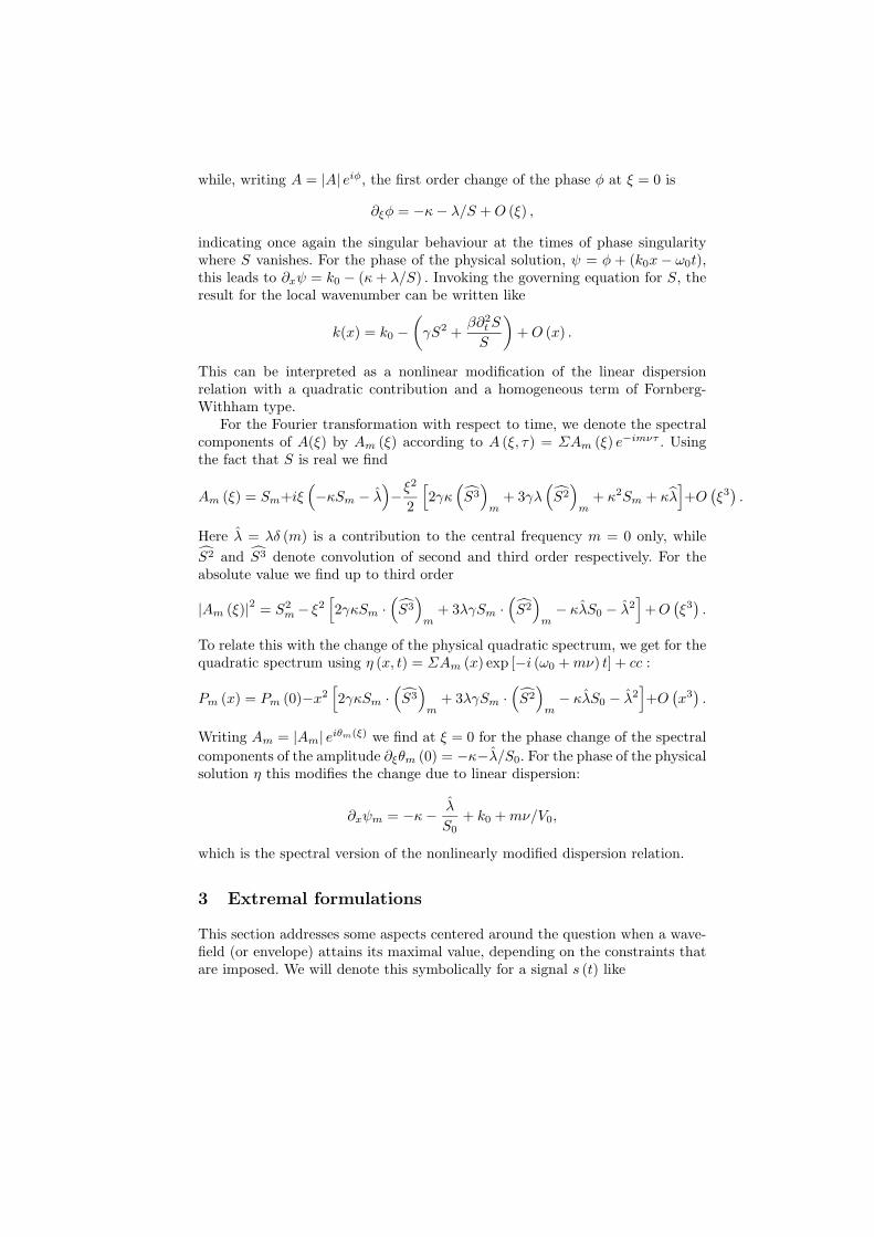
while, writing A = |A| eiφ, the first order change of the phase φ at ξ = 0 is
∂ξφ = −κ − λ/S + O (ξ) ,
indicating once again the singular behaviour at the times of phase singularitywhere S vanishes. For the phase of the physical solution, ψ = φ + (k0x − ω0t),this leads to ∂xψ = k0 − (κ + λ/S) . Invoking the governing equation for S, theresult for the local wavenumber can be written like
k(x) = k0 −(
γS2 +β∂2
t S
S
)+ O (x) .
This can be interpreted as a nonlinear modification of the linear dispersionrelation with a quadratic contribution and a homogeneous term of Fornberg-Withham type.
For the Fourier transformation with respect to time, we denote the spectralcomponents of A(ξ) by Am (ξ) according to A (ξ, τ) = ΣAm (ξ) e−imντ . Usingthe fact that S is real we find
Am (ξ) = Sm+iξ(−κSm − λ
)−ξ2
2
[2γκ
(S3
)
m+ 3γλ
(S2
)
m+ κ2Sm + κλ
]+O
(ξ3
).
Here λ = λδ (m) is a contribution to the central frequency m = 0 only, while
S2 and S3 denote convolution of second and third order respectively. For theabsolute value we find up to third order
|Am (ξ)|2 = S2m − ξ2
[2γκSm ·
(S3
)
m+ 3λγSm ·
(S2
)
m− κλS0 − λ2
]+O
(ξ3
).
To relate this with the change of the physical quadratic spectrum, we get for thequadratic spectrum using η (x, t) = ΣAm (x) exp [−i (ω0 + mν) t] + cc :
Pm (x) = Pm (0)−x2[2γκSm ·
(S3
)
m+ 3λγSm ·
(S2
)
m− κλS0 − λ2
]+O
(x3
).
Writing Am = |Am| eiθm(ξ) we find at ξ = 0 for the phase change of the spectral
components of the amplitude ∂ξθm (0) = −κ−λ/S0. For the phase of the physicalsolution η this modifies the change due to linear dispersion:
∂xψm = −κ − λ
S0+ k0 + mν/V0,
which is the spectral version of the nonlinearly modified dispersion relation.
3 Extremal formulations
This section addresses some aspects centered around the question when a wave-field (or envelope) attains its maximal value, depending on the constraints thatare imposed. We will denote this symbolically for a signal s (t) like

maxs
A (s) | constraints with A (s) = maxt
s (t)
In particular, the effect of prescribing the quadratic spectrum is considered first.Then we consider the case of relevance for the evolution of waves, when wetake as constraints motion invariants (integral quantities), and describe that theextreme signal of the SFB solutions of the previous section arises as special signalwhen the constraints are optimally chosen.
3.1 Constrained maximal signal amplitudes
Here we consider real functions of given period T and ν = 2π/T , or look atsignals with continuous spectrum (using the notation of the latter). Any signalwith given quadratic spectrum P (ω) is of the form
s (t) =
∫ √P (ω)eiθ(ω)e−iωtdω
for some phase function θ (ω). A completely focussed signal would have all phasesthe same, say zero, sfoc (t) =
∫ √P (ω)e−iωtdω, and produces the signal that
for the given quadratic spectrum has the largest amplitude (at t = 0), and
maxs
A (s) | s has given quadratic spectrum P (ω) = sfoc (0) =
∫ √P (ω)dω.
If we relax the constraints, the results critically depend on the constraints. Forinstance, if not the spectrum, but only the value of the integrated quadraticspectrum is prescribed, the related maximization problem has no finite solution.In Fourier language this is related to the fact that the energy is equally parti-tioned over all sidebands: equipartition of energy. We indicated in the previoussection that intermittent waves can partly contribute to a better equipartition.If stronger norms that the integrated quadratic spectrum are prescribed, finitesolutions will exist.
Most relevant seems to consider the maximization problem with constraintsthat are motivated by physics. To that end we introduce the following functionalsthat are related respectively to the approximation of the physical energy H, thephysical momentum I and the ‘mass’ functional M defined by
H (s) =
∫ T
0
[β
2(∂ts)
2 − γ
4s4
]dt, I (s) =
∫ T
0
1
2s2dt, M (s) =
∫ T
0
s dt,
and we investigate the optimization problem2
maxs
A (s) | H(s) = h; I(s) = g; M(s) = m . (2)
2 A very interesting statistically motivated variant of this maximization problem(without the linear mass-constraint) has been considered by Fedele [3]. He considersthe initial value problem (evolution in time) and uses the Hamiltonian and quadraticinvariant functionals that are related to the Zakharov equation, and takes as valuesof the constraints the values of a linearized wavefield at an initial time.

The resulting equation for (2) follows with Lagrange multiplier rule:
σδA = λ1δH + λ2δI + λ3δM (3)
where we write the variational derivative of a functional K like δK (when equatedto zero, δK = 0, this is precisely the Euler-Lagrange equation of the functionalK). The multipliers are related to the values of the constraints; when the rhsdoesn’t vanish, the multiplier σ can be taken equal to one without restriction.Explicitly, the equation reads
σδDirac (t − tmax(s)) = λ1
[−β∂2
t s + γs3]+ λ2s + λ3
where tmax(s) is the time at which s attains its maximum, and δDirac denotesDirac’s delta function. When the rhs vanishes, which is consistent with σ = 0,we recover the equation for the extremal signal of SFB described above. This isonly the case if the constraint values g, h,m are chosen correctly; we show inthe next subsection that this holds for the extremal signal.
For non-optimal constraint values, the multipliers will be different and σ 6= 0.Then formally the extremal signal can still be found explicitly but will not be arealistic physical signal since it contains a discontinuity in the derivative at thetime of maximal amplitude as a consequence of the delta-function; the optimalsolution is then obtained by pasting continuously together parts of a suitableextreme time signal. Although the signal itself may be non-physical, its value ofthe maximal amplitude provides an upperbound for any other signal satisfyingthe constraints.
3.2 Extremal property of the extreme signal
As stated above, among signals that satisfy constrained values of the functionalsH, I,M the ones with maximal amplitude will be obtained when the constraintsare such that these three functionals are linearly related (when σ = 0). We willnow show that the extremal signals have this property.
Indeed, for suitable parameters ν, r0 related to the constraint values g,m, theextreme signal will be a solution of the constrained optimization problem for thephysical energy
minS
H(S) | I(S) = g, M(S) = m (4)
Indeed, an extremizer of this optimization problem satisfies the Lagrangemultiplier formulation
δH(S) = −κδI(S) − λ (5)
for some multipliers −κ,−λ. Written in full for the specific functionals, this isprecisely the Newton equation (1) for the extreme signal. Actually, using thefact that H and I are restrictions to real-valued amplitudes of motion invariantsfor the complex amplitude of NLS, these values in (4) are immediately foundfrom the asymptotic values at the uniform wavetrain; we will describe this inmore detail in a forth coming paper [4].

4 Conclusions and remarks
We have studied a special class of wavefields and extracted several propertiesthat may be useful for the understanding of the appearance of extreme waves inmore realistic situations.
Although the wavefields are derived from the simple NLS-model and no rig-orous mathematical proof of their validity can be given, at least it can be saidthat these wavefields seem to be realizable in practice, as was shown by actualexperiments performed in large wavetanks at MARIN, see the contribution ofHuijsmans e.a. [5] in these proceedings. The experimental verification is vital, inparticular because most simplified models (and certainly NLS as has been usedhere) do not predict breaking phenomena. When breaking occurs, the determin-istic predictions become useless, while if no breaking occurs it can be expectedthat the predictions have qualitative, and as has been shown in the experiments,also quite good quantitative, validity.
It is also appropriate to discuss the validity, the ‘robustness’, of the basicphenomena described here for extension to more realistic situations. In particularthis concerns the optimization property of the extreme signal: can we expect sucha property to hold in more realistic situations, without relying on any convictionthat also in those cases ” ...... la nature agit selon quelque principe d’un maximumou minimum.” (Euler, 1746).
The optimization principle involves three functionals. Two of them have aclear physical meaning, although for NLS the complexified versions have to beconsidered. These are H, which is when complexified the Hamiltonian of NLSand is an approximation of the energy, and the quadratic functional I whichin complex form is also an NLS invariant that can be interpreted for the realwavefields as the momentum. These functionals will also be present as invari-ants for reliable models that are more accurate than the NLS model, since theenergy and momentum expressions are (approximations of) motion invariantsfor the full surface wave equations under the assumptions of non viscous fluidand translation symmetry. It can therefore be anticipated, or at least it can behoped, that these two functionals will be relevant in any optimization principlefor realistic large waves at the extreme position.
The major questionable point in the idea to generalize (4) is the role of theso-called ‘mass’ functional M that does not seem to correspond to a physicallywell understood invariant functional in more general situations. From its defini-tion, M (S) is seen to be precisely the square root of the energy in the centralfrequency, M (S) = S0. It will be shown in [4] that this ‘mass’ turns up as aspecial case, valid only at the extreme position, in a variational principle thatdescribes the complete SFB evolution as a relative equilibrium according to gen-eral Hamiltonian theory. That variational formulation depends on (the existenceof) a higher order invariant functional, and this seems to be related to the spe-cial properties of the completely integrable NLS equation considered here. Sothe results presented here do not unambiguously support the idea that the op-timization principle for the extreme signal can be expected to hold also in more

realistic cases. Yet it is tempting to look for such extremal formulations also inmore realistic cases.
It may even be possible to investigate in a direct way the optimization prin-ciple for the extreme signal from experiments in a well-controlled laboratoryenvironment. One possibility is to calculate the values of the relevant function-als from the measured signal at the extreme position, and investigate how closethese values are near the optimal values from the minimizing property. Another,less robust (and therefore maybe more informative) method may be to use thefact that the extremizing property reflects itself in a simple phase-plane rep-resentation of the signal, see [2], so that the phase plane representation of theexperimental extreme signals could give an indirect indication. Further researchin this direction will be executed.
Acknowledgement
Regular discussions with Gert Klopman (UTwente) and Renee Huijsmans(MARIN) have been helpful. Special thanks to Francesco Fedele for referringto [3] and some useful discussions. Financial support from RUTI (Ministry ofResearch and Technology, Indonesia) in the project ‘Wave motion and Simu-lation’, and support for visits to ITB of EvG and NK by EU-Jakarta projectSPF2004/079-057, and for visit of NK to ’Rogue Waves 04’ by JMBurgers Cen-tre, is acknowledged. This work is also part of project STW 5374 ‘ExtremeWaves’ from the technology division STW of NWO Netherlands.
References
1. N.N. Akhmediev and A. Ankiewicz, Solitons, Nonlinear pulses and beams, Chapman& Hall, 1997
2. Andonowati, N. Karjanto and E. van Groesen, Extreme wave phenomena in down-stream running modulated waves, submitted July 2004.
3. F. Fedele, The occurence of extreme wave crests and the nonlinear wave-wave in-teraction in random sea; Proceedings XIV ISOPE Conference, Toulon, France, May2004..
4. E. van Groesen and Andonowati, Variational formulations for extreme waves, to bepublished.
5. R.H.M. Huijsmans, G. Klopman, N. Karjanto and Andonowati: Experiments onextreme wave generation based on Soliton on Finite Background; in Proceedings
‘Rogue Waves 2004’, Brest France, October 2004.6. P. Janssen, Nonlinear four-wave interaction and freak waves, JPO 33 (2003) 863-884

Dependence of Freak Wave Occurrence
on Kurtosis
Nobuhito Mori1 and Peter A.E.M. Janssen2
1 Osaka City University,Department of Environmental Urban Engineering,
3-3-138 Sugimoto, Sumiyoshi-ku, Osaka 558-8585, [email protected]
2 European Centre for Medium-Range Weather Forecasts,Shineld Park, Reading RG2 9AX, UK
Abstract. The occurrence probability of freak waves is formulated asa function of number of waves and surface elevation kurtosis based onthe weakly non-Gaussian theory. Finite kurtosis gives rise to a signi-cant enhancement of freak wave generation. For xed number of waves,the estimated amplication ratio of freak wave occurrence due to thedeviation from the Gaussian theory is 50%-300%.
1 Introduction
The last decade freak waves have become an important topic in engineering
and science. Freak wave studies started in the late 80’s [1] and the high-order
nonlinear eects on freak waves were discussed in the early 90’s [2, 3]. Due
to many research eorts, the occurrence of freak waves, their mechanism and
detailed dynamical properties are now becoming clear [4, 5, 6, 7, 8]). It was
concluded that the third order nonlinear interactions enhance the freak wave
occurrence and are the primary cause of freak wave generation in a general wave
eld except for the case of strong wave-current interaction or wave diraction
behind an island [9].
Numerical and experimental studies have demonstrated that freak-like waves
can be generated frequently in a two-dimensional wave ume without current,
refraction or diraction [2, 4, 6, 10]. Moreover, the numerical studies clearly in-
dicate that a freak wave having a single, steep crest can be generated by the
third order nonlinear interactions in deep-water [2]. Also, the theoretical back-
ground of freak wave generation has become more clear [5], but the quantitative
occurrence probabilities on the ocean surface remain uncertain. In addition, it
is still questionable how to characterize the dominant statistical properties of
freak wave occurrence in terms of nonlinear parameters, spectral shape, water
depth and so on.
Recently, Janssen [11] investigated the freak wave occurrence as a conse-
quence of four-wave interactions including the eects of non-resonant four-wave

2 Mori and Janssen
interactions. He formulated the analytical relationship between the spectral
shape and the kurtosis of the surface elevation. These results have the potential
to unify the previous freak wave studies covering nonlinear interactions, spectral
proles, nonlinear statistics, etc.
The purpose of this study is to investigate the relationship between kurtosis
and the occurrence probability of freak wave in a unidirectional wave train. First,
the wave height distribution is formulated as a simple function of kurtosis by the
non-Gaussian theory. Second, the maximum wave height distribution is obtained
from the wave height distribution as a function of kurtosis and number of waves.
Finally, the dependence of the occurrence probabilities of freak waves on kurtosis
and the number of waves will be analyzed and discussed.
2 Theoretical Formulation of Freak Wave Occurrence
Following a central limit theorem, linear, dispersive random waves have a Gaus-
sian probability distribution function (PDF) for the surface elevation. Finite
amplitude eects result, however, in deviations from the Normal distribution, as
measured by a nite skewness and kurtosis. For narrow band wave trains it will
be shown that the wave height distribution only depends on the kurtosis. There-
fore, we shall formulate the relationship between wave height distribution and
kurtosis to examine analytically the eects of kurtosis on freak wave occurrence.
We assume that waves to be analyzed here are unidirectional with narrow
banded spectra and satisfy the stationary and ergodic hypothesis. Let η(t) be
the sea surface elevation as a function of time t and ζ(t) an auxiliary variable
such that η(t) and ζ(t) are not correlated. Assuming both η(t) and ζ(t) are real
zero-mean functions, we have
Z(t) = η(t) + iζ(t) = A(t)eiφ(t), (1)
A(t) =√
η2(t) + ζ2(t), (2)
φ(t) = tan−1
ζ(t)
η(t)
, (3)
where A is the envelope of the wave train and φ the phase. For weakly nonlinear
waves deviations from the Normal distribution are small. In those circumstances
the PDF of the surface elevation can be described by the Edgeworth distribu-
tion, and the joint probability density function of η and ζ is known. The PDF of
the envelope A now follows immediately from an integration of the joint prob-
ability distribution over the phase φ. It is then found that the rst term gives
the Rayleigh distribution, while the terms involving the skewness and etc, all
integrate to zero because they are odd functions of the phase. The third term
does give contributions to the probability distribution for the envelope and as a
result we nd
p(A) = Ae−12 A2
[
1 +1
4(κ40 + κ22)
1 − A2 +1
8A4
]
, (4)

Dependence of Freak Wave Occurrence on Kurtosis 3
where κij is joint cumulant between η and ζ and we have used κ40 = κ04,
a relation that can easily be veried. Following Mori and Janssen [12], κ22 =
κ40/3 and the nal result for the narrow-band approximation of the PDF of the
envelope becomes
p(A) = Ae−12 A2
[
1 +1
3κ40
1 − A2 +1
8A4
]
. (5)
From this result interesting consequences on the distribution of maximum wave
heights may be obtained. In the narrow band approximation wave height Hequals 2A and hence the wave height PDF becomes
p(H) =1
4He−
18 H2
[1 + κ40AH(H)] , (6)
where AH(H) = 1384
(
H4 − 32H2 + 128)
. The exceedance probability PH (H) for
wave height then follows from an integration of the wave height PDF from H to
∞:
PH(H) = e−18 H2
[1 + κ40BH(H)] , (7)
where BH(H) = 1384H2
(
H2 − 16)
.
We adopt a simple freak wave denition. A freak wave is thought to occur
when the maximum wave height Hmax exceeds twice the signicant wave height
H1/3 of the wave train. The PDF of maximum wave height pm in wave trains
can be obtained once the PDF of wave height p(H) and exceedance probability
of wave height P (H) is known [13], thus,
pm(Hmax)dHmax = N0[1 − P (Hmax)]N0−1p(Hmax)dHmax. (8)
Substitution of Eqs.(6) and (7) into Eq.(8), gives the PDF of the maximum wave
height, pm,
pm(Hmax)dHmax =N
4Hmax e−
H2max
8 [1 + κ40AH(Hmax)]
× exp
−Ne−H
2max
8 [1 + κ40BH(Hmax)]
dHmax, (9)
and exceedance probability of the maximum wave height Pm,
Pm(Hmax) = 1 − exp
−Ne−H
2max
8 [1 + κ40BH(Hmax)]
. (10)
Eq.(9) is now evaluated as a function of N and κ40 (or µ4). For κ40 = 0 results
are identical to the ones following from the Rayleigh distribution. For simplicity
it will be assumed that H1/3 = 4ηrms (with ηrms the square root of the mean
of the surface elevation variance). The freak wave condition therefore becomes
Hmax/ηrms ≥ 8, and we obtain from Eq.(10) the following simple formula to
predict the occurrence probability of the freak wave as a function of N and κ40,
Pfreak = 1− exp [−N(1 + 8κ40)] (11)

4 Mori and Janssen
102
103
104
10−2
10−1
100
N
Pfr
eak
Rayleighµ
4 = 3.1
µ4 = 3.2
µ4 = 3.3
µ4 = 3.4
µ4 = 3.5
Fig. 1. Occurrence probability of freak wave as a function of number of waves N andkurtosis µ4.
where = e−8.
Figure 1 shows for increasing µ4 from 3.0 to 3.5 the comparison between
the linear (Rayleigh) theory and present theory of the occurrence probability of
the freak wave, Pfreak , as a function of the number of waves N . For the case
of N=100, the occurrence probability of the freak wave predicted by the linear
theory is 3.3%, while it is 15.4% according to Eq.(9) with µ4=3.5, and for the
case of N=1000, the occurrence probability of the freak wave is 28.5% by the
linear theory, while it is 81.3% according to Eq.(9) with µ4=3.5. Thus, freak
waves in a strong nonlinear eld can occur several times more frequently than
in a linear wave eld, which obeys the Rayleigh distribution.
Figure 2 shows the ratio of freak wave occurrence probability Rfreak pre-
dicted by the present theory and the Rayleigh theory, as a function of kurtosis
µ4. For the case of a small number of waves N 250, the ratio Rfreak linearly
depends on µ4. If µ4 is 3.1 and N 500, the occurrence probability of freak
waves is 50% (two times) more than according to linear theory. On the other
hand, the increment of Rfreak decreases as the number of waves increases. This
is because for very large number of waves even in linear theory the maximum
wave height almost always exceeds 2 × H1/3.
3 Conclusion
In this study, the kurtosis and related high-order cumulants were evaluated on
the basis of Janssen’s work [11]. Second, the wave height and the maximum wave

Dependence of Freak Wave Occurrence on Kurtosis 5
3 3.1 3.2 3.3 3.4 3.50
50
100
150
200
250
300
350
µ4
Rfr
eak [
%]
N=100 N=250 N=500 N=1000 N=5000
Fig. 2. Ratio of freak wave occurrence predicted by Eq.(11) to the Rayleigh theory.
height distribution were formulated as a function of kurtosis. Finally, the freak
wave occurrence probability was formulated as a function of kurtosis and number
of waves. From the theoretical frame work, we have the following remarks.
– The second order cross-cumulant between surface elevation and its envelope,
κ22, is 1/3 of the fourth cumulant, κ40, of the surface elevation.
– The weakly non-Gaussian theory shows the dependence of the maximum
wave height distribution on kurtosis.
– The occurrence probability of freak waves is signicantly enhanced by the
kurtosis increase as a consequent of the wave-wave interactions.
In order to check the validity of the theories developed here, systematic and
continuous eld measurement of freak waves will be critically required.
References
[1] R.G. Dean. Freak waves: a possible explanation. In A. Tørum and O.T. Gudmes-tad, editors, Water wave kinematics, pages 609–612. Kluwer Academic Pub., 1990.
[2] T. Yasuda, N. Mori, and K. Ito. Freak waves in a unidirectional wave train andtheir kinematics. In Proc. of the 23th Int. Conf. on Coastal Eng., volume 1, pages751–764, Venice, 1992. ASCE.
[3] T. Yasuda and N. Mori. High order nonlinear eects on deep-water random wavetrains. In International Symposium: Waves-Physical and Numerical Modelling,volume 2, pages 823–332, Vancouver, 1994.
[4] K. Trulsen and K. Dysthe. Freak waves-a three-dimensional wave simulation.In Proceedings of the 21st Symposium on Naval Hydrodynamics, pages 550–558.(National Academy Press, 1997.

6 Mori and Janssen
[5] A.R. Osborne, M. Onorato, M. Serio, and S. Bertone. The nonlinear dynamicsof rogue waves and holes in deep water gravity wave trains. Physical Letter A,(275):386–393, 2000.
[6] Onorato M., A.R. Osborne, M. Serio, and S. Bertone. Freak waves in randomoceanic sea states. Physical Review Letter, (86):5831–5834, 2001.
[7] Sverre Haver. Evidences of the existence of freak waves. In M. Olagnon andG. Atanassoulis, editors, Rogue Waves, pages 129–140. 2001.
[8] N. Mori, P. Liu, and T. Yasuda. Analysis of freak wave measurements in the Seaof Japan. Ocean Engineering, 29(11):1399–1414, 2002.
[9] M. Olagnon and G. Athanassoulis, editors. Rogue Waves. IFRMER, 2000.[10] C.T. Stansberg. Extreme waves in laboratory generated irregular wave trains. In
A. Tørum and O.T. Gudmestad, editors, Water wave kinematics, pages 573–590.Kluwer Academic Pub., 1990.
[11] P.A.E.M. Janssen. Nonlinear four-wave interactions and freak waves. J. Phys.
Oceanogr., (33):2001–2018, 2003.[12] N. Mori and P.A.E.M Janssen. On kurtosis and occurrence probability of freak
waves. in preparation, 2005.[13] Y. Goda. Random Seas and Design of Maritime Structures. World Scientic, 2nd
edition, 2000.

Extreme Events 1
Extreme Events in Field Data and in a Second Order Wave Model
Elzbieta Maria Bitner-Gregersen1, and Anne Karin Magnusson2
1 Det Norske Veritas, Veritasveien 1, N-1322 Høvik, Norway
[email protected] 2 Norwegian Meteorological Institute, Allégaten 70,
N-5007 Bergen, Norway [email protected]
Abstract. The analysis is based on North Sea field data and on second order time domain simulations. Statistical properties of extreme waves are presented. Particu-lar focus is given to the wave crest. Wave parameters obtained from the field data are compared with the values derived from the second order time domain simula-tions. Limitations of the 2nd order wave model to predict extreme events are shown. Uncertainties related to the field and numerically generated data are dis-cussed.
1 Introduction
Abnormal waves, often called rogue waves or freak waves have been subject to much attention recently. These waves represent operational risks to ship and offshore struc-tures, and are likely to be responsible for a number of accidents in the past. The com-pleted (in 2003) EU research project MaxWave has made significant contribution to the understanding of freak waves; however, several important questions are still not an-swered. Too few data sets including freak events have been recorded making difficult to develop satisfactory physical and statistical models for prediction of these waves. Fur-ther, no consensus has been reached neither about a definition of a freak event nor about the probability of occurrence of freak waves. Finally, still more research is called for in order to investigate effects of these waves on marine structures.
The random nature of sea surface and non-linear effects are important when analyz-
ing extreme events. Higher order solutions increase wave steepness, maximum crest and wave height compared to linear theory, and consequently also increase the probability of occurrence of extreme waves. As shown by several authors (i.e. [17], [9], [2]), freak waves in the “second order world” are pretty rare events. At the 100-year crest level the 2nd order models are expected to be of reasonable accuracy to predict extreme events, see [4].

Extreme Events 2
The present analysis is based on North Sea field data and on second order time do-main simulations using measured sea state parameters. The study focuses on statistical properties of extreme waves and on limitations of the 2nd order wave model to predict them. Main attention is given to the wave crest. Time series of wave elevations are gen-erated using the Pierson-Moskowitz [16], JONSWAP [9] and two-peak Torsethaugen [19] frequency spectral shapes for long-crested seas and deep/intermediate water depth. Measured wave parameters are compared with values given by the second order time domain simulations. Sampling variability related to the data is discussed.
2 Field Data
Fig. 1 The North Sea with locations of Ekofisk, Varg, Draupner, Sleipner, Frigg and
Gullfaks. Field data from two sites (Ekofisk and Draupner) in the North Sea are used. The follow-ing storms have been chosen as background for the study:
(1) 25-26 October 1998: The ‘Stenfjell case’, using data at Ekofisk. The case is named after the bulk carrier Stenfjell, which arrived at Esbjerg (a harbour on West coast of Denmark) on the morning of 26 October 1998 with heavy weather damage to the wheelhouse, accommodation and electrical installations, reportedly due to freak waves. The ship was sailing from Hamburg to Tananger (near Stavanger, Western Norway). The ship experienced wind and waves from a low that had passed over the central North Sea, giving strong winds in a constricted area on the South of the low. The area moved from the East of Scotland towards the Danish coast passing over Ekofisk where a sharp increase in wave height (Hs=10m) was observed on the 25th. Some high crests are measured by lasers at two locations of the site and are analysed further herein.

Extreme Events 3
(2) 27 December 1998: A situation with close to 12m significant wave height with westerly winds at Ekofisk. High crests are observed in measured time series. The fetch is short from this direction and the increase is sharp. (3) 5-6 February 1999: The production ship (FPSO) at Varg (58N, 2E), operated by Saga Petroleum, experienced some damage due to ‘green water’ [5]. The wave damage caused the loss of a life buoy, a fire equipment storage locker torn from the connections and minor damages to cable gates occurred. All these items were located at the mid-ship. Time of incidence is not known. At Ekofisk, about 160 km further South, waves increased rapidly from 5 to 9m in a 6 hours period, with winds from between W and WNW. Wind speed stayed thereafter stable around 22-25 m/s during the night (a 12 hour period), slackening a little (to 20-23 m/s). At around 4 a.m. the 5th, wind direction veered to NNW and a high crest is recorded at Ekofisk at 04:40 UTC. (4) 30 November 1999: FPSO Varg B experienced some damage due to ‘green water’ [5]. Norsk Hydro reported damage to gas sensors, fire hose cabinets, doors on deluge stations for chemical injection module. Time of incident is not known, but records at Ekofisk also give some high crests. One record with Crx/Hs = 1.4 is used in this study, which occurred in the growing phase of the storm. The record is discussed further below. (5) 29-30 January 2000: the Petrojarl Varg ship, operated by Norsk Hydro, experienced damage on fore ship, midship and aft ship [5]. The incident is regarded as the most critical event so far on the Norwegian sector. The strong winds in the South area of the low pressure also influenced Ekofisk. Wave heights increased to about 11m. Some high crests are observed when wind speed is at its maximum (25 m/s from 17 to 21 UTC, from 280 deg). At that time it is most likely that waves are unidirectional. (6) 1 January 1995: The ‘Draupner wave’ with a crest height of 18.5 m above mean sea level is recorded by Statoil at the Draupner platform [11]. During this storm several wave heights (trough- to crest heights) more than twice Hs were observed at the Frigg platform operated by Elf Aquitaine. Analysis of weather maps indicates that there is swell added onto the wind sea from a slightly different direction.
The storms listed above have been selected from the MaxWave storm database [14].
Note that apart of the Draupner January 1 event all storms were recorded at the Ekofisk platform (see Fig.1). Sampling frequency used at Ekofisk is 2Hz, at Draupner 2.133 Hz. There are three sensors at Ekofisk: a waverider, and 2 downlooking lasers; the laser data are used herein. Wave data at Draupner are measured with a laser. The water depth for both platforms is 70m. One to two wave records (see Table 1) with the most extreme events present have been chosen from each storm and analyzed herein. In Table 1 H4std denotes significant wave height calculated from the time series and is equal to 4 times standard deviation of the sea surface while Hm0 represents significant wave height ob-tained from the zero-spectral moment of the whole time series. Although recognized

Extreme Events 4
software is used to calculate H4std and Hm0, a significant difference between the two estimators can be observed.
Table 1. Wave records selected for the study.
Case Date and time H4std (m) Hm0 (m) Tp (s) Tm02 (s) 1 25 Oct. 1998, 16:00 UTC 9.2 8.8 12.6 9.2 2 27 Dec. 1998, 06:40 UTC 11.6 10.4 14.6 10.6 3 5 Feb. 1999, 04:40 UTC 8.1 7.6 13.0 9.1 4 1 Dec. 1999, 02:20 UTC 6.5 7.2 11.3 8.7 5 29 Jan. 2000, 18:40 UTC 10.5 12.1 12.2 8.8 6 1 Jan. 1995, 15:20 UTC 11.9 11.2 16.7 10.8 7 1 Jan. 1995, 23:00 UTC 6.1 5.7 9.8 6.9
3 Second Order Simulations
A simulation program documented by Birknes and Bitner-Gregersen [1] is applied. Time series of wave elevations are generated using three empirical spectra: Pierson-Moskowitz [16], JONSWAP [9] and Torsethaugen [19]. The wave amplitudes are given by
θωθθω ∆∆= )(),(2 DSa (1)
in the case of a directional sea state. Assuming single peaked frequency spectrum, e.g. JONSWAP, the spectrum can be given as S(ω,θ)= S(ω) D(θ) . For a two-peaked spec-trum, we use S(ω,θ)= S1(ω) D1(θ)+S2(ω) D2(θ). S1 and S2 may represent swell and wind sea frequency spectra and D1 and D2 are corresponding spreading functions.
Random wave amplitudes and random phases are generated for each wave compo-nent. The phases are assumed uniform distributed on the interval [0,2π], and the ampli-tudes are Rayleigh distributed with mean-square value given by
[ ] ωω ∆= )(22 SaE (2)
The wave amplitude and phase define the complex wave amplitude through the fol-lowing relation
)exp( εiaA = (3)
A convenient model for combined seas is simply to add two frequency spectra
)()()( fSfSfS wsw += (4)
where Ssw(f) is the swell spectrum and Sw(f) is the wind sea spectrum .

Extreme Events 5
The Torsethaugen two-peak spectrum applied herein was established primarily for one location (Statfjord, the Northern North Sea) but in qualitative terms is expected to be of much broader validity, and is currently used by the Norwegian industry for loca-tions exposed to North Atlantic swell. The spectrum is an average wave spectrum de-rived by introducing various empirical factors, and therefore it should not be used un-critically for other locations. An attractive feature of the Torsethaugen spectrum is that only limited information about the sea-state is required as the spectrum is completely defined given the significant wave height and spectral peak period. The model splits the energy into a swell component and wind-sea component, using a modified JONSWAP spectrum for both peaks. It is noticed that even though including contribution from wind sea and swell the Torsethaugen spectrum does not necessarily need to have two pronounced peaks. In the Torsethaugen model, each sea state is classified as swell dominated sea or wind dominated sea according to the criterion:
fp
fp
TTifwindseaTTifswell
≤>
where 3/1moff HaT =
(5)
where pT is the peak period, and 6.6=fa is adopted from the JONSWAP experiment [9]. If fp TT ≤ , the local wind-sea dominates the spectral peak, if fp TT > the swell dominates the spectral peak.
The statistical results presented herein are based on 350 simulations of a 1024 sec timeseries at 4Hz for the long-crested sea. A 1024 sec timeseries includes approxi-mately 90-120 wave cycles. The chosen number of simulations gives reasonably stable results [3]. Typically the analyzed parameters evaluated from the simulations have ap-proximately constant values for number of simulations N>250. The calculations are carried out for the Torsethaugen spectrum and JONSWAP assuming peak enhancement factor γ equal to 3.3 and 1.0 (Pierson-Moskowitz). Results for deep/intermediate water depth are reported herein (water depth 70m).
4 Comparison of Wave Characteristics
Different definitions of freak waves are proposed in the literature. Often used as a characteristic is that the factor Hmax/Hs>2 (maximum crest to trough wave height factor). A ratio larger than 2 is seldom to be found in measured data, especially when measured by buoys due to the typical lack of skewness in these data [12, 13]. But this factor may not always be sufficient for an operational definition of an extreme or freak wave. Another commonly advocated definition of freak waves is a criterion based on the factor Cmax/Hs, e.g. as suggested by Haver and Andersen [11] that Cmax/Hs>1.2 within a 20-minute sea elevation time series. Tomita and Kawamura [18] suggest that both a wave height and a crest height criterion be simultaneously fullfilled, with the height factor

Extreme Events 6
higher than 2 and the crest factor higher than 1.3. Guedes Soares et al.[7, 8] argue that use of the height factor and the crest factor is not sufficient.
All wave records chosen for the present study include an event c/Hs >1.2 and are shown in Figures 2-8. In each figure the top panel represents the 20 minutes time series sampled at 2Hz including the crest event analysed. Lower left panel shows the time history of significant wave height, maximum crest and trough in each 20minutes records during the storm. Lower right panel shows the frequency spectrum from the time series shown in top panel, using Blackman-Harris windowing and Fourier analysis on all data (nfft=2395, nb of samples), thereafter averaging the spectrum over 5 frequency bins (Nfa=5).
Fig. 2 Case 1: Measurements from laser at Flare South at Ekofisk during 25. Octo-ber 1998. Lower left panel: Blue line: significant wave height using H4std, red line: max crest height (Crx) in each 20 minute record, black line: inverse of deepest trough (Trx) measured in each 20min record. Cmax/H4std = 1.29 at 16:00 UTC
As seen in these figures the extreme events appear at different times of the storm his-
tories, before, at, and after the significant wave height culmination (referred to here as part of storm with the highest sH ). Further, as shown in Table 2, by applying the Tor-sethaugen criterion (Eq.(5)) only the Draupner wave record (sea sate 6, Tp=16.7s) repre-sents clearly swell dominated sea. The sea state measured in case 2 (27 December 1998, 06:40 UTC) with Tp=14.6s, is very slightly swell dominated (Tp > Tf ) when Hm0 is used in calculation of Tf and wind dominated when H4std is used. The relation between Tp and

Extreme Events 7
Tf calculated from the spectra in the other cases (1, 3, 4, 5 and 7) indicates that the sea state is wind dominated following the Thorsethaugen criterion.
Fig.3 Case 2: 27 December 1998 storm . Cmax/H4std = 1.24 at 06:40 UTC.
Fig.4 Case 3: 5-6 February 1999 storm. Cmax/H4std = 1.31 at 04:40 UTC the 6th.
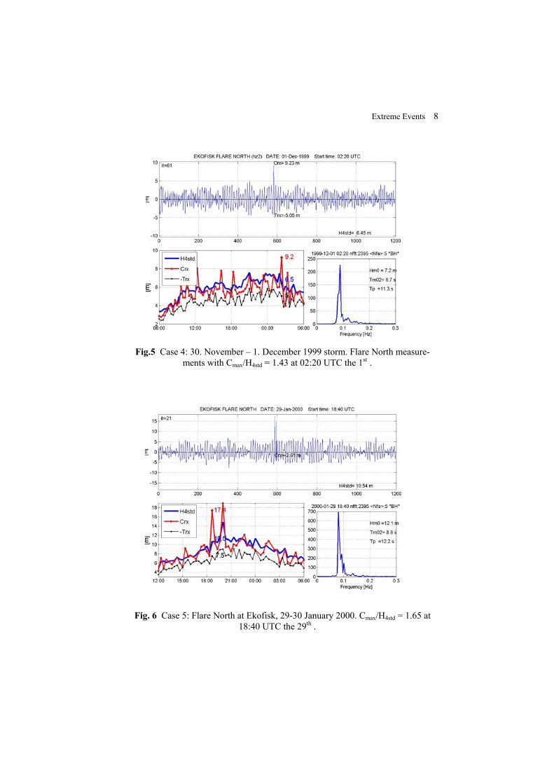
Extreme Events 8
Fig.5 Case 4: 30. November – 1. December 1999 storm. Flare North measure-
ments with Cmax/H4std = 1.43 at 02:20 UTC the 1st .
Fig. 6 Case 5: Flare North at Ekofisk, 29-30 January 2000. Cmax/H4std = 1.65 at 18:40 UTC the 29th .

Extreme Events 9
Fig. 7 Case 6: The Draupner “New year wave” recorded during the 1 Jan. 1995 storm, at 15:20UTC. Lower left panel shows the crest in detail. Cmax/H4std = 1.55
Fig. 8 Case 7: Second case from the Draupner platform on 1 Jan. 1995 storm, 23:00UTC. (Cmax/H4std = 1.75).

Extreme Events 10
As expected (see Table 1) different crest to height ratios (Cmax/Hs) are obtained using
either H4std or Hm0, and the difference between the ratios is significant for some wave records (see Table 2). Use of H4std or Hm0 may decide whether an event is classified as a freak event or not. Herein H4std has been adopted because further discussions on which standard spectral analysis method to use is outside the scope of this paper.
Table 2. Sea surface characteristics.
Field data Simulations – PM* Sea state
Tp (s)
Tf* (s)
Tf**(s) Cmax
(m) Cmax
/H4std
Cmax
/ Hm0 E[Cmax ] σcmax
(m) E[Cmax ] /H4std
1 12.6 13.8 13.6 11.8 1.29 1.34 8.47 2.91 0.92 2-w/sw d. 14.6 14.9 14.4 14.4 1.24 1.38 10.62 3.26 0.91 3 13.0 13.3 13.0 10.6 1.31 1.39 7.31 2.71 0.90 4 11.3 12.3 12.7 9.20 1.43 1.28 5.88 2.43 0.91 5 12.2 14.5 15.1 17.4 1.65 1.44 10.04 3.17 0.95 6-swell d. 16.7 15.1 14.8 18.50 1.55 1.65 10.53 3.25 0.88 7 9.8 12.0 11.8 10.63 1.75 1.86 5.76 2.20 0.95 * H4std , ** Hm0 The second order simulations have been carried out using water depth of 70m, as-
sumption of long-crested sea and H4std and Tp as an input. Tp will depend on the averag-ing method used in the spectral calculations. In Table 2 results from simulations assum-ing a Pierson-Moskowitz (PM) spectrum are presented. Figs. 9 and 10 show results from simulations using all 3 types of spectral shapes (PM, JONSWAP and Thorsethaugen). In Fig.9 the mean and mean + 2*std of simulated extreme crests are compared with obser-vations, while in Fig. 10 the mean and the maximum values of simulated maximum crests are compared with the maximum observed crests.
The JONSWAP spectrum with the factor γ equal to 3.3 gives lower mean extreme
crest in comparison to the Pierson-Moskowitz and Torsethaugen spectrum in all cases. This can be attributed, in average, to larger spectral width for the two latter spectra, than the JONSWAP spectrum for the sea states considered, see also [4]. Further, we can see that the Torsethaugen spectrum increases slightly the extreme crests in average for the Draupner sea state 6, but, however, reduces the standard deviation. For the PM spec-trum the mean extreme crest obtained from the 2nd order time domain simulations is up to 43% lower compared to the maximum observed crest. For the last 3 cases ( 5 (Janu-ary 2000), 6 (Draupner 1995, 15:20UTC) and 7 (Draupner 1995, 23:00UTC)), the ob-served maximum crest is outside the interval range of the simulated mean of extreme crests plus two standard deviations of the extreme crest distribution, particularly for the higher sea states 5 and 6 (10.5m and 11.9m, compared to 6.1m in case 7). This confirms

Extreme Events 11
the earlier findings presented in the literature; the freak wave observed at Draupner cannot adequately
Extreme Wave Crest
Simulated and Field data
0
5
10
15
20
0 1 2 3 4 5 6 7 8 9 10Sea state
Extr
eme
cres
t (m
)
PM extreme mean
PM ext. mean +2std.
JONS extreme mean
JONS ext. mean +2std
Torst. extreme mean
Tors. ext. mean+2std.
Max. observed
Fig. 9 Extreme wave crests in the 6 storm cases. Blue filled circles are observations.
For simulations assuming Pierson-Moskowitz, JONSWAP and Thorsethaugen spectral shapes: given here are mean of maximum crests (points are all below observations) and its value + twice the standard deviation (see legend for symbol and color).
Extreme crest
0
5
10
15
20
0 1 2 3 4 5 6 7 8 9 10Sea state
Cre
st (m
)
PM extreme meanPM max. simulatedJONS extreme meanJONS max simulatedTors. extreme meanTors. max. simulatedMax. observed
Fig. 10 As for Fig. 9, but simulation results are shown with mean and maximum val-ues of maximum crest.

Extreme Events 12
be accounted for by the 2nd order model. Note that the wave crest in the case 5 can be put in doubt due to the form (Fig. 11) of the wave behind the crest. However, for the less extreme events in cases 1 to 4 where Cmax/Hs <1.45, the 2nd order model ‘captures’ the observed maximum wave crest, thus the maximum observed crest is close to the crest extreme mean plus two standard deviations, see also [3].
Fig. 11 Measured wave profiles in the extreme observed crests of case 1 to 7 ( increasing from left to right, top to bottom). In case 5 the second peak is obviously a spike value. The shape of the first peak (case 5) may also be a spike but is analyzed herein.
The simulation results reported in Figs. 9 and 10 are based on the nominal (ob-
served) significant wave height, Hs,nom. However, as pointed out by Bitner-Gregersen and Hagen [3] for a sample of 17 minutes time series there is a scatter in the spectral variance caused by sampling variability, which is accounted for in the simulations through random spectral amplitudes. For time series of 17 minutes duration, the coeffi-cient of variation for significant wave height for a sample of realizations is in the range

Extreme Events 13
5-7% (Olagnon & Magnusson [15] also showed Hm0 calculated from simulations varied with up to 9%, in the mean 6%).
A high value of Cmax/Hs,nom may occur in a sea state in which also the simulated sig-nificant wave height is high (Hs,sim = 4*standard deviation of 2048 simulated wave eleva-tion values). In this case, Cmax/Hs,sim would be lower than Cmax/Hs,nom. On the other side, a high crest observed in a 3 hour sea state may very well occur in a part of the sea state where the 20 minutes averaged significant wave height is substantially higher than the 3 hour averaged Hs, making the factor Cmax/Hs,nom low. In Fig. 10, the maximum simulated and observed wave crests are shown while Fig. 12 illustrates the difference between Cmax /Hs,nom and Cmax/Hs,sim for the PM spectrum. As can be observed, there is a clear differ-ence, and this aspect should be kept in mind when evaluating freak criteria based on Cmax /Hs or Hmax/Hs ratios.
Crest criterion Cmax/H4std
0
0,4
0,8
1,2
1,6
2
0 1 2 3 4 5 6 7 8Sea state
Cm
ax/H
4std
Field dataSimul. Hs nonimalSimul. Hs simulated
Fig. 12 Wave crest factor for nominal and simulated significant wave height using PM spectral shape.
5 Summary of Discussion
Cases analyzed herein show that the ratio Cmax/Hs may vary significantly depending upon whether the significant wave height is calculated from the time series H4std (4 times standard deviation) or from the zero-spectral moment Hm0. Which formulae is used may influence on deciding whether an event is classified as a freak wave or not. It is recommended to use both significant wave estimates with care, and investigate them further if significant difference between them is observed.

Extreme Events 14
Cases 1 to 4 with the less extreme waves (Cmax/Hs <1.45) are well ‘captured’ by the 2nd order wave model. By capture it is meant here that the observed maximum crest is close to the simulated mean of extreme crests plus two standard deviations of the ex-treme crest distribution. This could be utilized in design by calibrating the extreme mean crest calculated by the 2nd order wave model. There is though no assurance that the ob-servations have captured the most extreme waves in the area around Ekofisk due to changing profiles as waves evolve [13].
When Cmax/Hs >1.45, particularly for higher sea states with Hs>10.0m, the observed
maximum crest is outside the interval range of the simulated mean of extreme crests plus two standard deviations for the records characterized. Using the Torsethaugen crite-rion [19] to define the sea state to be wind sea or swell, we find that two of these cases have been recorded in wind dominated sea (January 2000 storm, Draupner sea state at 23:00UTC) and the third one, the Draupner wave 1. January 1995 at 15:20UTC, in a swell dominated sea. Simulations of the Draupner wave assuming the Thorsethaugen spectral shape gives slightly higher mean values of the extreme crests as compared to PM or JONSWAP shapes.
In the first four cases, JONSWAP shapes give lower mean values, and PM shapes
give highest extremes. Differences are though within decimetres.
The above leeds to the conclusion that spectral shapes do influence results but a ques-tion is how significant these differences are. Further investigations are required to reach a firm conclusion.
It must be noted that of the 7 cases considered, the first 4 high crests occurred at end of the culmination period, when wind has relaxed to slightly lower speed, and wind direction is in a veering situation. This indicates that the sea state might be bi-directional at the event. Case 5, which is probably a spike, occurs in a strong growth phase of the storm (in which sea spray is highly probable). Cases 6 and 7 are a bit more difficult to define weatherwise (wavewise). Wind was around 20m/s all afternoon in the Northern North Sea, but analysis of weather maps also indicate the high crest events at both 15 and 23 occur in a slackening situation in the wind field as the wind direction is veering slowly towards North. Again one might find a spectrum with large spread or bi-directionality in these cases.
The present analysis is limited to long-crested sea. Further investigations including
directional effects are called for.
Acknowledgement
The work presented was performed partially within the EU - Project “Safety and Reli-ability of Industrial Products, Systems and Structures” (SAFERELNET), which is de-scribed in http://mar.ist.utl.pt/saferelnet/ and is funded partially by the European Com-

Extreme Events 15
mission under the contract number G1RT-CT2001-05051 of the programme “Competi-tive Sustainable Growth”.
References
1. Birknes. J. and Bitner-Gregersen. E.M.: Non-linearity of the Second-order Wave Model for Directional Two- Peak Spectra. Proc. ISOPE’2003 Conf. Hawai. (2003).
2. Bitner-Gregersen, E. M.: Sea state duration and probability of occurrence of a freak crest. Proc. OMAE’2003 Conf., Cancun, Mexico (2003).
3. Bitner-Gregersen. E.M. and Hagen. Ø.: Effects of Two-Peak Spectra on Wave Crest Statistics. Proc. OMAE’2003 Conf., Cancun, Mexico (2003).
4. Bitner-Gregersen, E. M., and Hage, Ø.: Freak Waves in the Second Order Wave Model. OMAE’2004 Proc., Vancouver, Canada (2004).
5. Ersdal, G. and A. Kvitrud,: Green water incidents on Norwegian production ships. Proceedings of ISOPE’2000 (2000).
6. Forristall. G. Z.: Wave Crests Distributions: Observations and Second-Order Theory. J. Physical Oceanography, vol.30. No.8. pp.1931-1943. (2000)
7. Guedes Soares, C., Cherneva, Z., and Antao, E.M., “Characterisrics of Abnormal Waves in North Sea Storm Sea States. Accepted for publication in J. Applied Ocean Research (2004a).
8. Guedes Soares, C., Cherneva, Z., and Antao, E.M.: Abnormal Waves during Hurricane Camille. Accepted for publication in J. Geophysical Research (2004b).
9. Hasselmann. K. and Co-authors: Measurements of Wind-wave Growth and Swell Decay during the Joint North Sea Wave Project (JONSWAP). Dtsch. Hydrogr. Z.. Suppl. A. Vol.8. (1973).
10. Hagen, Ø.: Statistics for the Draupner January 1995 Freak Wave Event. Proc. OMAE-2002 Conference, Oslo, Norway (2000).
11. Haver, S. and Andersen O. J.: Freak Waves. “Rare Realizations of a Typical Popula-tion or Typical Realizations of a Rare Population.”. ISOPE’ 2000, Seattle (2000).
12. Longuet-Higgins, M.S.: Eulerian and Lagrangian aspects of surface waves. J. Fluid Mech. 173, 683-707, (1986).
13. Magnusson, A. K, M. A. Donelan and W. M. Drennan: “On estimating extremes in an evolving wave field.” Coastal eng. 36, pp 147-163 (1999).
14. Magnusson, A. K., Bitner-Gregersen, E.M. and Nieto Borge, J.C.: Analysis of Ex-treme Waves in the Maxwave Database. WMO Proc. Geneva (2003).
15. Olagnon, M, and A. K. Magnusson, 2004: “Sensitivity study of sea state parameters in correlation to extreme wave occurrences”. In proceedings of 14th international Offshore and Polar Engineering conf., ISOPE 3, (2004).
16. Pierson, W.J. and Moskowitz, L.: A proposed Stectral Form for Fully developed Wind Seas based on the Similarity Theory of tA.A. Kitaigorodskii. J. Geoph. Res. Vol 69, pp 5181-5190 (1964).
17. Prevosto, M. and Bouffandeau, B.: Probability of Occurrence of a “Giant” Wave Crest. Proc. OMAE-2002 Conference, Oslo, Norway (2002).

Extreme Events 16
18. Tomina, H. and Kawamura, T.: Statistical Analysis and Inference from the In-Situ Data of the Sea of Japan with Reference to Abnormal and/or Freak Waves. Proc. ISOPE’2000 Conf., Seattle, USA (2000).
19. Torsethaugen, K.: Model for Double Peaked Wave Spectrum. SINTEF Civil and Environmental Engineering, Rep. No. STF22 A96204, Trondheim, Norway (1996).

Spectral parameters to characterize the risk of
rogue waves occurrence in a sea state
Michel Olagnon and Anne Karin Magnusson
IFREMER Centre de Brest BP F Plouzane France Norwegian Meteorological Institute Allegaten Bergen Norway
Abstract In a previous paper we discussed the natural variability of some spectral parameters that may characterize a sea state andconcluded that deviations that might be observed close to occurrencesof extreme waves were well within the natural range of variability As aconsequence prediction of increased risk of rogue waves occurrence cannot be made from a simple local examination of the spectrum but wouldrequire investigation of either simultaneous values of several parametersor of the time history of a parameter over durations of the same order ofmagnitude as a stormIn the present study we investigate that second possibility ie since theexcursions on the timescale of a seastate are not decisive we considerthe next timescale that of a whole storm To this aim the Frigg database is searched for storms and an attempt is made to select within theset of storms a subset of freaky storms where there are observationsof high crests with respect to the prevailing signicant wave height Thehistories of spectral parameters during the storms are then computedand dierences from histories in the subset and some other storms sincethe other storms cannot all be freaky are sought forSimilarly to the previous study those parameters are preferred thatmight be related to rogue wave occurrence They were determined eitherfrom theoretical wave considerations BenjaminFeir instability indicators or from meteorological ones spectral front bandwidth that mightreveal running fetch situations
Introduction
Signicant wave heightHS peak period Tp and main wave direction are sucientto describe sea states for most practical purposes However that information isclearly not sucient to detect increases in the risk of occurrence of unexpectedrogue waves in a sea state We thus study observations of additional parametersin hope that on one hand they exhibit special properties when rogue waves occurand that on the other hand they can be related to some theoretical mechanism ofrogue wave generation and thus validate the assumption that the correspondingmechanism is active in nature on those occasions when rogue waves are observed
It should be noted that in order to be useful a parameter must have acharacteristic change for some duration at a signicantly larger timescale than

that of the individual wave Otherwise the change in the parameter would merelybe a detection of the rogue wave and could not be used for forecast nor wouldit mean anything more than the wrong place at the wrong time and it thuscould not fully validate a particular generation mechanism
The next higher timescale that of a stationary sea state was investigatedin a previous paper We concluded that sea state spectral parameters thatexhibit sensitivity to rogue wave occurrences
do not depart from the normal range of aleatory variations but show onlyslight biases and
exhibit a high rate of false alarm
We recommended that one try to nd out criteria based on combined occurrenceof several characteristics including directional ones or based on the next highertimescale ie the process or the timehistory of characteristics over a wholestorm duration
The present study investigates the latter suggestion that of characteristicsderived from a whole storm
Ersdal and Kvitrud report on a total of storms in the North Seaand for two of them damage was observed at two dierent locations Similarlydamage was also reported at a BP platform during the storm of the famousNew Year Wave It is thus not unlikely that storms as a whole might havesome characteristics related to an increase in the risk of occurrence of roguewaves
BenjaminFeir Instability indices
Many authors put forward nonlinear focusing as a generating mechanism forrogue waves and suggest to characterize it through an index of the BenjaminFeirinstability BFI computed by dividing steepness by adimensional bandwidth
Results reported in and recalled in gure show that though sea stateBFI indices are biased towards higher values when rogue waves occur that biasis of little practical value since a small BFI index is no garantee that roguewaves will not occur and alerts for of the rogue waves would require tosend warnings more than half of the time
Yet the high natural variability of BFI index might be a consequence ofthe diculty to obtain stable estimators when considering short in situ recordsespecially with respect to that part of spectral bandwidth that is relevant to theBenjaminFeir instability and that is focused on the spectral peak
Goda recognizes that the narrowness parameter Qp and the otherones that are based on spectral moments are sensitive at least to some extent tothe tail of the spectrum andor the cuto frequency used in the measurementsand analysis He suggests the use of normalized peak height p Sfpfpm
as a measure of the sharpness of the spectral peakThat measure of bandwidth has several advantages

BFr
0.00 0.02 0.04 0.06 0.08 0.10 0.12 0.14 0.16 0.18 0.20
number
0.00
200.00
400.00
600.00
800.00
1000.00
1200.00
1400.00
1600.00
1800.00
2000.00
Cmax/Hm0 > 1.1 Cmax/Hm0 > 1.25
BFr
0.00 0.02 0.04 0.06 0.08 0.10 0.12 0.14 0.16 0.18 0.20
number
0.00
10.00
20.00
30.00
40.00
50.00
60.00
70.00
80.00
Fig Histogram of the robust BenjaminFeir index values for sea states atFrigg
it is not signicantly aected by the cuto frequency or a poor estimationof the spectral tail and of its shape
it enables to dene in the same manner a spectral front bandwidth fpusing the restriction of m to fp
it enables to dene a spectral asymetry coecient that is also free from theinuence of the spectral tail AS p fpp
That denition is often discarded because of the diculties in estimatingpresisely Smax especially for measured spectra However a resonable amount ofrobustness may be achieved by using in such cases the weighted average of the

Flare North StenfjellBFj
0.00 5.00 10.00 15.00 20.00 25.000.00
0.20
0.40
0.60
0.80
1.00
1.20
1.40
0.00
1.25
2.50
3.75
5.00
6.25
7.50
8.75
10.00
11.25
12.50
0.95
1.10
1.25
1.40
Flare North StenfjellBFr
0.00 5.00 10.00 15.00 20.00 25.000.00
0.05
0.10
0.15
0.20
0.25
0.00
1.25
2.50
3.75
5.00
6.25
7.50
8.75
10.00
11.25
12.50
0.95
1.10
1.25
1.40
Flare North StenfjellBFm
0.00 5.00 10.00 15.00 20.00 25.000.00
0.05
0.10
0.15
0.20
0.25
0.30
0.35
0.00
1.25
2.50
3.75
5.00
6.25
7.50
8.75
10.00
11.25
12.50
0.95
1.10
1.25
1.40
Fig Timehistory of crests dashed red normalized crests red circles BF Indexblack dots and its and aleatory variability fractiles solid blue
peak value and of its two neighbours The following relationships then hold
Save Simax Simax Simax
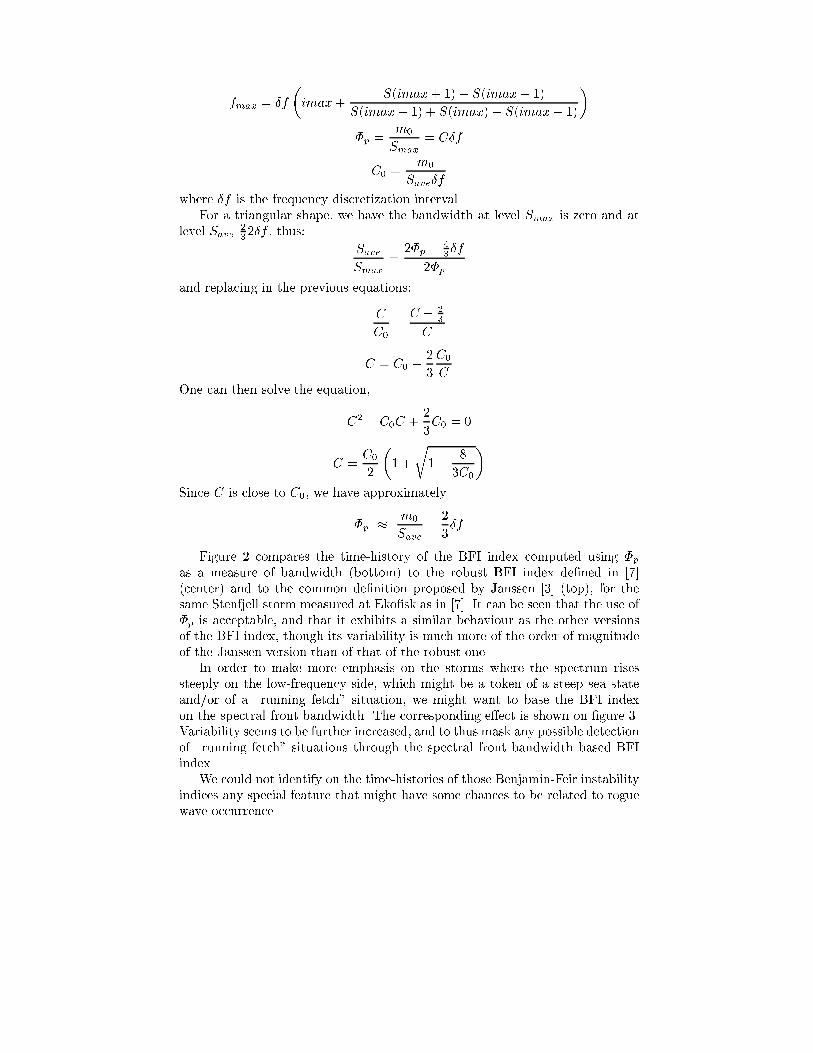
fmax f
imax
Simax Simax
Simax Simax Simax
p m
Smax
Cf
C m
Savef
where f is the frequency discretization intervalFor a triangular shape we have the bandwidth at level Smax is zero and at
level Save
f thus
SaveSmax
p
f
p
and replacing in the previous equations
C
C
C
C
C C
C
C
One can then solve the equation
C CC
C
C C
r
C
Since C is close to C we have approximately
p m
Save
f
Figure compares the timehistory of the BFI index computed using pas a measure of bandwidth bottom to the robust BFI index dened in center and to the common denition proposed by Janssen top for thesame Stenfjell storm measured at Ekosk as in It can be seen that the use ofp is acceptable and that it exhibits a similar behaviour as the other versionsof the BFI index though its variability is much more of the order of magnitudeof the Janssen version than of that of the robust one
In order to make more emphasis on the storms where the spectrum risessteeply on the lowfrequency side which might be a token of a steep sea stateandor of a running fetch situation we might want to base the BFI indexon the spectral front bandwidth The corresponding eect is shown on gure Variability seems to be further increased and to thus mask any possible detectionof running fetch situations through the spectral front bandwidth based BFIindex
We could not identify on the timehistories of those BenjaminFeir instabilityindices any special feature that might have some chances to be related to roguewave occurrence
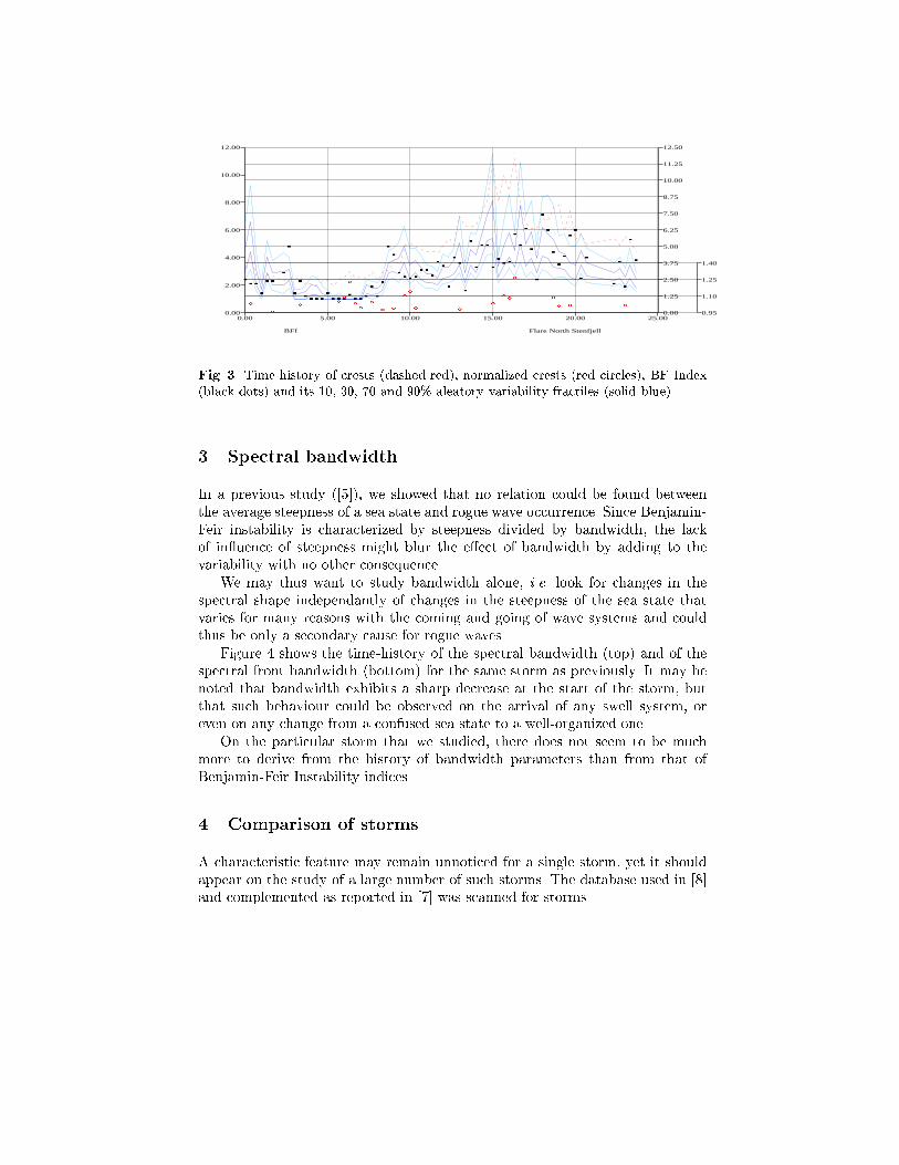
Flare North StenfjellBFf
0.00 5.00 10.00 15.00 20.00 25.000.00
2.00
4.00
6.00
8.00
10.00
12.00
0.00
1.25
2.50
3.75
5.00
6.25
7.50
8.75
10.00
11.25
12.50
0.95
1.10
1.25
1.40
Fig Timehistory of crests dashed red normalized crests red circles BF Indexblack dots and its and aleatory variability fractiles solid blue
Spectral bandwidth
In a previous study we showed that no relation could be found betweenthe average steepness of a sea state and rogue wave occurrence Since BenjaminFeir instability is characterized by steepness divided by bandwidth the lackof inuence of steepness might blur the eect of bandwidth by adding to thevariability with no other consequence
We may thus want to study bandwidth alone ie look for changes in thespectral shape independantly of changes in the steepness of the sea state thatvaries for many reasons with the coming and going of wave systems and couldthus be only a secondary cause for rogue waves
Figure shows the timehistory of the spectral bandwidth top and of thespectral front bandwidth bottom for the same storm as previously It may benoted that bandwidth exhibits a sharp decrease at the start of the storm butthat such behaviour could be observed on the arrival of any swell system oreven on any change from a confused sea state to a wellorganized one
On the particular storm that we studied there does not seem to be muchmore to derive from the history of bandwidth parameters than from that ofBenjaminFeir Instability indices
Comparison of storms
A characteristic feature may remain unnoticed for a single storm yet it shouldappear on the study of a large number of such storms The database used in and complemented as reported in was scanned for storms

Flare North StenfjellBwd
0.00 5.00 10.00 15.00 20.00 25.000.00
0.10
0.20
0.30
0.40
0.50
0.60
0.70
0.80
0.90
0.00
1.25
2.50
3.75
5.00
6.25
7.50
8.75
10.00
11.25
12.50
0.95
1.10
1.25
1.40
Flare North StenfjellBwdf
0.00 5.00 10.00 15.00 20.00 25.000.00
0.05
0.10
0.15
0.20
0.25
0.30
0.35
0.00
1.25
2.50
3.75
5.00
6.25
7.50
8.75
10.00
11.25
12.50
0.95
1.10
1.25
1.40
Fig Timehistory of crests dashed red normalized crests red circles Bandwidthblack dots and its and aleatory variability fractiles solid blue
Storms are dened as durations of at least consecutive hours where significant wave height remains above meters Those storms were identied on thetwo dierent datasets of the database the synthetic parameters computed byOceanor on the measurements carried out on the eld and the values computedat Ifremer from the available timeseries at QP The Oceanor data cover the period from January to March That period contains storms ofwhich are also present in the data at Ifremer for which timerecords of the watersurface elevation are available with a Hz sampling frequency as measured witha radar distancemeter from the QP platform on the Frigg eld
A typical example of timehistories of the bandwidth parameters during aFrigg storm is given in gure Comparison over several storms can be made
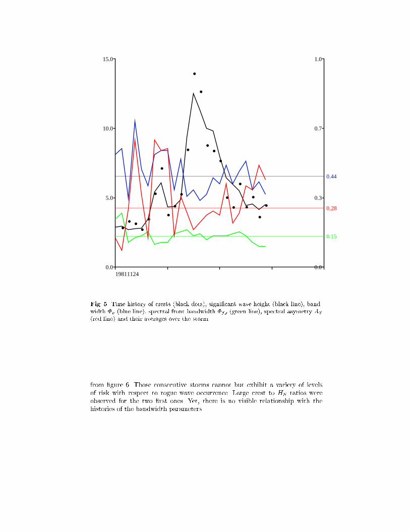
198111240.0
5.0
10.0
15.0
0.0
0.3
0.7
1.0
0.44
0.15
0.28
Fig Timehistory of crests black dots signicant wave height black line bandwidth p blue line spectral front bandwidth fp green line spectral asymetry AS
red line and their averages over the storm
from gure Those consecutive storms cannot but exhibit a variety of levelsof risk with respect to rogue wave occurrence Large crest to HS ratios wereobserved for the two rst ones Yet there is no visible relationship with thehistories of the bandwidth parameters

19811124
0.0
5.0
10.0
15.0
0.0
0.3
0.7
1.0
0.44
0.15
0.28
19811204
0.0
5.0
10.0
15.0
0.0
0.3
0.7
1.0
0.48
0.14
0.37
19811220
0.0
5.0
10.0
15.0
0.0
0.3
0.7
1.0
0.37
0.12
0.32
19820226
0.0
5.0
10.0
15.0
0.0
0.3
0.7
1.0
0.37
0.12
0.36
19820310
0.0
5.0
10.0
15.0
0.0
0.3
0.7
1.0
0.35
0.12
0.32
19820408
0.0
5.0
10.0
15.0
0.0
0.3
0.7
1.0
0.40
0.150.23
Fig Timehistories of crests black dots signicant wave height black line bandwidth p blue line spectral front bandwidth fp green line spectral asymetry AS
red line and their averages over the storms
Conclusions
The present study shows that dimensionless parameters related to spectral shapeare rather constant over all storms in the database as could be hinted from theresults of another previous study
As for the height and period or steepness it was shown at the previousRogue Waves workshop that steepness does not have any inuence on theprobability of rogue wave occurrence and that signicant wave height has onlya limited one
The timehistory of spectral parameters evolution during a storm seems thusnot to be a good candidate for the denition of warning systems Furthermoreone may wonder about the validity of the assumption that some storms aremore prone to extreme waves than others or at least about the fact that such acharacteristic would be reected in the nondirectional wave spectra
Should the asumption be invalidated ie extreme waves have no higher probability to happen in some storms than in any other then either rogue waveswould be normal extremes of the distribution conrming some previous results

obtained by Robin Olagnon on a subset of the database investigated hereeither it would mean that the dataset is still too small for the dierences toappear or that the storm characteristics that are related to abnormal extremesshould be sought elsewhere than in the spectrum
References
Ersdal G Kvitrud A Green sea on Norwegian production shipsProc Airgap Workshop HSEEP Forum London
Goda Y Analysis of Wave Grouping and Spectra of Longtravelled SwellReport of the Port and Harbour Research Institute Vol No pp
Janssen PAEM Nonlinear four wave interactions and freak wavesTechnical Memorandum ECMWF
Olagnon M Krogstad HE Observed short and longterm distributions of wave steepness Proc Int Oshore and Polar Engineering Conf Vol Montreal pp
Olagnon M van Iseghem S Some Cases of Observed Rogue Wavesand an Attempt to Characterize their Occurrence Conditions Proc Rogue Waves
Ifremer Actes de Colloques pp Olagnon M Representativity of some standard spectral models for
waves Proc th International Oshore and Polar Engineering Conf ISOPE pp
Olagnon M Magnusson AK Sensitivity Study of Sea State Parameters in Correlation to Extreme Wave Occurrences Proc th International
Oshore and Polar Engineering Conf ISOPE Robin A Olagnon M Occurrence of Extreme Waves with respect to
Signicant Wave Height Proc Oshore Mechanics and Artic Engineering OMAEVola pp

Experiments on extreme wave generationusing the Soliton on Finite Background
Rene H.M. Huijsmans1, Gert Klopman2,3, Natanael Karjanto3, andAndonawati4
1 Maritime Research Institute Netherlands, Wageningen, The Netherlands,e-mail: [email protected]
2 Albatros Flow Research, Marknesse, The Netherlands3 Applied Analysis and Math. Physics, Univ. of Twente, Enschede, The Netherlands
4 Jurusan Matematika, Institut Teknologi Bandung, Bandung, Indonesia
Introduction
Freak waves are very large water waves whose heights exceed the significant waveheight of a measured wave train by a factor of more than 2.2. However, this initself is not a well established definition of a freak wave. The mechanism of freakwave generation in reality as well as modeling it in a wave basin has become anissue of great importance.Recently one is aware of the generation of freak wave through the Benjamin–Feirtype of instability or self–focussing. Consequently the Non–Linear–Schrodinger(NLS) equation forms a good basis for understanding the formation of freakwaves. However, the complex generation of a freak wave in nature within a seacondition is still not well understood, when the non-linearity of the carrier waveis not small. In our study we will focus on the Soliton on Finite Background,an exact solution of the NLS equation, as a generating mechanism for extremewaves.Apart from a numerical investigation into the evolution of a soliton on a fi-nite background also extensive detailed model tests have been performed forvalidation purposes in the hydrodynamic laboratories of the Maritime ResearchInstitute Netherlands (marin). Furthermore, a numerical wave tank [12] is usedto model the complete non-linear non-breaking wave evolution in the basin.
Properties of the Soliton on Finite Background
The NLS equation is chosen as a mathematical model for the non-linear evolutionof the envelope of surface wave packets. For spatial evolution problems, it is givenin non-dimensional form and in a frame of reference moving with the groupvelocity by
∂ξψ + iβ∂2τψ + iγ|ψ|2ψ = 0, (1)
where ξ and τ are the corresponding spatial and temporal variables, respectively;β and γ are the dispersion and non-linearity coefficients. This equation has many

2
families of exact solutions. One family of exact solutions is known as the Solitonon Finite Background (SFB) and this is a good candidate for describing extremewaves. This exact solution has been found by Akhmediev, Eleonskii & Kulagin[3], see also [2] and [1].
This SFB solution describes the dynamic evolution of an unstable modu-lation process, with dimensionless modulation frequency ν. In the context ofwater waves, for infinitesimal modulational perturbations to a finite-amplitudeplane wave, this process is known as Benjamin-Feir (BF) instability [5]. How-ever, non-linearity will limit this exponential growth and the SFB is one (ofmany other) non-linear extension of the BF instability for larger amplitudes ofthe modulation. Extensive research on the NLS equation and the SFB solution,to obtain a better understanding of deterministic extreme-wave phenomena hasbeen conducted in the past few years (see e.g. [10], [11], [4] and [9]).
An explicit expression for the SFB is given as the following complex-valuedfunction
ψ(ξ, τ ; ν, r0) = A(ξ) ·
ν2 cosh(σξ)− i[σ/(γr20)
]sinh(σξ)
cosh(σξ)−√
1− 12 ν
2 cos(ντ)− 1
, (2)
where A(ξ) = r0e−iγr2
0ξ is the plane-wave or the continuous wave solution of theNLS equation, σ = γr20 ν
√2− ν2 is the growth rate corresponds to the Benjamin-
Feir instability, ν = ν r0√
γβ is the modulation frequency, and ν, 0 < ν <
√2 is
the normalized modulation frequency. This SFB reaches its maxima at (ξ, τ) =(0, 2nπ
ν
), n ∈ Z. It has a soliton-like form with a finite background in the spatial
ξ-direction. The SFB is periodic along in the temporal τ -direction, with period2πν . For |ξ| → ∞, the SFB turns into the continuous wave solution A(ξ). It
possesses two essential parameters: r0 and ν.
Fig. 1. Density plots of a physical wave packet profile according to an SFB envelopefor ν1 = 1, showing the wave dislocation phenomenon.

3
The first-order part of the corresponding physical wave packet profile η(x, t)for a given complex-valued function ψ(ξ, τ) is expressed as follows
η(x, t) = ψ(ξ, τ)ei(k0x−ω0t) + c.c., (3)
where c.c. means the complex conjugate of the preceding term, the wave numberk0 and frequency ω0 satisfy the linear dispersion relation ω = Ω(k) ≡
√k tanh k.
The variables (x, t) in the non-moving frame of reference are related to (ξ, τ) inthe moving frame of reference by the transformation ξ = x and τ = t−x/Ω′(k0).The modulus of ψ represents the wave group envelope, enclosing the wave packetprofile η(x, t). The dimensional laboratory quantities are related to the non-dimensional quantities by the following Froude scaling, using the gravitionalacceleration g and the depth of the basin h: xlab = x·h, tlab = t·
√gh , klab = k/h,
ωlab = ω ·√
gh , and ηlab = η · h.
In principle, the wave profile including the higher-order terms represents agood approximation to the situation in real life. To accommodate this fact, wewill include higher-order terms up to second order. We apply an perturbation-series expansion (Stokes’ expansion) to the physical wave-packet profile η(x, t)and the multiple-scale approach using the variables ξ and τ , where ξ = ε2x, τ =ε(t−x/Ω′(k0)), and ε is a small positive non-linearity and modulation parameter.The corresponding wave elevation η(x, t), consisting of the superposition of thefirst-order harmonic term of O(ε) and a second-order non-harmonic long waveas well as a second-order double-frequency harmonic term of O(ε2), is given by
η(x, t) = ε[ψ(10)(ξ, τ)ei(k0x−ω0t) + c.c.
]+ ε2
ψ(20)(ξ, τ) +
[ψ(22)(ξ, τ)e2i(k0x−ω0t) + c.c.
]. (4)
We find from the multiple-scales perturbation-series approach that ψ(10)(ξ, τ) =ψ(ξ, τ) satisfies the spatial NLS equation and
ψ(20)(ξ, τ) = − 1Ω(k0)
4k0Ω′(k0)−Ω(k0)
[Ω′(0)]2 − [Ω′(k0)]2|ψ(10)(ξ, τ)|2 (5)
ψ(22)(ξ, τ) = k03− tanh2 k0
2 tanh3 k0
[ψ(10)(ξ, τ)]2. (6)
A similar derivation for the temporal NLS equation resulting from the KdVequation can be found in [8]. By including this second-order term, the wave signalη(x, t) experiences the well-known Stokes’ effect: the crests become steeper andthe troughs becomes shallower [6].
The coefficients β and γ of the spatial NLS equation are given, in non-dimensional form, as:
β = −12Ω′′(k0)
[Ω′(k0)]3, (7)
γ =γ1 + k0αU + λαζ
Ω′(k0), (8)

4
where
γ1 = k20Ω(k0)
9 tanh4 k0 − 10 tanh2 k0 + 94 tanh4 k0
, (9)
λ =12k20
1− tanh2 k0
Ω(k0), (10)
αζ = − 1Ω(k0)
4k0Ω′(k0)−Ω(k0)
[Ω′(0)]2 − [Ω′(k0)]2and (11)
αU = αζΩ′(k0)−
2k0
Ω(k0). (12)
These can be used to compute the SFB solution ψ(ξ, τ) from Equation (2).
Phase singularity and wave dislocation
By writing the complex-valued function ψ in a polar (or phase-amplitude) repre-
sentation, it is found that for modulation frequencie ν in the range 0 < ν <√
32
a phase singularity phenomenon occurs. It happens when the real-valued am-plitude |ψ| vanishes and therefore there is no way of ascribing a value to thereal-valued phase when it occurs. The local wave number k ≡ k0 +∂xθ and localfrequency ω ≡ ω0 − ∂tθ, with θ(ξ, τ) ≡ arg (ψ(ξ, τ), become unbounded whenthis happens. The corresponding physical wave packet profile η(x, t) confirmsthis by showing a wave dislocation phenomenon. When the real-valued ampli-tude |ψ| vanishes at that specific position and time, waves merge or split. For√
32 < ν <
√2, the real-valued amplitude is always definite positive, and thus
there is no wave dislocation. Furthermore, in one modulation period, there is apair of wave dislocations. Before or after this dislocation, the real-valued ampli-tude reaches its maximum value. Figure 1 shows the density plot of a physicalwave packet profile η(x, t). The wave dislocation is also visible in this figure.Figure 2 shows the evolution of the SFB from a modulated wave signal until itreaches the extreme position. We can see also in this figure that the amplitude|ψ| vanishes at some moments for the extremal position x = 0, causing phasesingularity.
The phase singularity is a well known phenomenon in physical optics. Inthe context of water waves, similar observations can be made, and also wavedislocations occur. Trulsen [13] calls it as crest pairing and crest splitting andhe explains this phenomenon as a consequence of linear dispersion.
Maximum temporal amplitude
The maximum temporal amplitude (MTA) is a useful concept to understandlong-time behavior of wave elevation. For wave propagation in the laboratory,it also gives a direct view of the consequences of an initial wave signal on thecorresponding extreme-wave signal. It is defined as
µ(x) = maxt η(x, t), (13)

5
where η(x, t) is the surface elevation as a function of space x and time t. Itdescribes the largest wave elevation that can appear at a certain position. Forlaboratory wave generation, it describes the boundary between the wet and dryparts of the wall of the basin after a long time of wave evolution.
Figure 3 shows the MTA plot of the SFB in the laboratory coordinates. In thisexample, the mean water depth is 3.55 m and the wavelength is approximately6.2 m. The wave signal is generated at the left side, for example at xlab = −350m, and it propagates to the right and reaches its extremal condition at xlab = 0.A slightly modulated wave train increases in amplitude as the SFB waves travelsin the positive x-direction. Furthermore, in this example a SFB wave signal withinitial amplitude around 0.19 m can reach an extreme amplitude of 0.45 m, anamplification factor of around 2.4. After reaching its maximum amplitude, theMTA decreases monotonically and returns to its initial value.
Experimental Result
For the validation of the proposed method we performed experiments in one ofthe wave basins of marin. The basin dimensions amounted to L × B × D as200 m × 4.0 m × 3.55 m. In the basin an array of wave probes were mounted asindicated in the set–up in figure (4). The predefined wave board control signalwas put onto the hydraulic wave generator. The stroke of the wave flap wasmeasured. Main characteristics of the model test experiments:Carrier wave period is 1.685 sec. maximum wave height to be achieved (MTA)varies from 0.213m to 0.2485mAs a explanation the results for the tests with an MTA of 0.2485 will be shown,see figure( 5) to figure(7).
Figure 8 shows the SFB signal based on the experiment at distance 150 mfrom the wave maker, where it is expected that the signal to be extreme. Thatfigure also shows the phase singularity phenomenon when the local frequencybecomes unbounded when the real-valued amplitude vanishes or almost vanishes.The experiment result shows asymmetric form of the extreme signal while thetheoretical result of the SFB preserve the symmetry of the signal. It is suspectedthat if the modified NLS equation of Dysthe [7] is used as the governing equationfor the wave signal evolution, then there are good comparisons with experimentalmeasurements. The good comparisons are observed for the case of bi-chromaticwaves, where the modified NLS equation predicts both the evolution of individualwave crests and the modulation of the envelope over longer fetch [14].
References
1. Akhmediev, N.N. & Ankiewicz, A. “Solitons, Nonlinear Pulses and Beams”,
Optical and Quantum Electronic Ser., Vol. 5, Chapman & Hall, 1st edition, (1997).2. Akhmediev, N.N. & Korneev, V.I. “Modulation instability and periodic so-
lutions of the nonlinear Schrodinger equation”, Theor. and Math. Phys. Vol. 69,(1986), pp. 1089–1092.

6
3. Akhmediev, N.N., Eleonskii, V.M. & Kulagin, N.E., “First-order exactsolutions of the nonlinear Schrodinger equation”, Teoret. Mat. Fiz., Vol. 72, No. 2,(1987), pp. 183–196. English translation: Theoret. and Math. Phys., Vol. 72, No. 2,(1987), pp. 809–818.
4. Andonowati, Karjanto, N. & van Groesen, E., “Extreme wave phenomenain down-stream running modulated waves”, submitted to Math. Models and Meth.in Appl. Sc., July, (2004).
5. Benjamin, T.B. & Feir, J.E., “The disintegration of wave trains on deep water.Part 1. Theory”, J. Fluid Mech., Vol. 27, No. 3, (1967), pp. 417–430.
6. Debnath, L., “Nonlinear Water Waves”, Academic Press, (1994).7. Dysthe, K.B., “Note on a modification to the nonlinear Schrodinger equation for
application to deep water waves”, Proc. R. Soc. London Ser. A, Vol. 369, No. 1736,(1979), pp. 105–114.
8. van Groesen, E., “Wave groups in uni-directional surface-wave model”, J. Eng.Math., Vol. 34, No. 1-2, (1998), pp. 215–226.
9. van Groesen, E., Andonowati & Karjanto, N., “Deterministic aspects of non-linear modulational instability”, In: Proc. ‘Rogue Waves’, Brest, France, October,(2004).
10. Osborne, A.R., Onorato, M. & Serio, M. “The nonlinear dynamics of roguewaves and holes in deep-water gravity wave trains”, Phys. Lett. A, Vol. 275, (2000),pp. 386–393.
11. Osborne, A.R., “The random and deterministic dynamics of ‘rogue waves’ inunidirectional, deep-water wave trains”, Mar. Struct., Vol. 14, (2001), pp. 275–293.
12. Westhuis, J.H., “The numerical simulation of non–linear waves in a hydrody-namic model test basin”, Ph.D. Thesis, University of Twente, (2001).
13. Trulsen, K., “Crest pairing predicted by modulation theory”, In J. Geophys. Res.,Vol. 103, No. C2, pp. 3143–3147.
14. Trulsen, K. & Stansberg, C.T., “Spatial evolution of water surface waves:Numerical simulation and experiment of bichromatic waves”, In Proc. EleventhInt. Offshore and Polar Eng. Conf., The Int. Soc. of Offshore and Polar Eng.,(2001), pp. 71–77.

7
−30 −10 10 30
Fig. 2. The evolution of the SFB for ν1 = 1 from a modulated continuous wave signalinto the extreme position. From top to bottom, the signals are taken at x = −200,x = −100, x = −50, x = −30, and x = 0.

8
−350 −300 −250 −200 −150 −100 −50 0 50 100
−0.45
−0.15
0.15
0.45
x
Fig. 3. The MTA plot of the SFB, the corresponding wave profiles at t = 0, and itsenvelope.
10m
40m
100m
150m
200m
4.0m
Fig. 4. The set-up of the wave probe array in the wave basin

9
Fig. 5. Comparison Non-Linear Wave model HUBRIS with results from experimentsand sNLS
Fig. 6. Comparison Non-Linear Wave model HUBRIS with results from experimentsand sNLS

10
Fig. 7. Comparison Non-Linear Wave model HUBRIS with results from experimentsand sNLS
150 200 250 300 350 400−0.3
−0.1
0.1
0.3
t [s]
η(x,t)
Extreme signal, x = 150 m, M = 28.73 cm, with predicted M = 21.30 cm, ν~ = 1
150 200 250 300 350 400
0
100
200
300
400
t [s]
ω(x,t)
Local frequency, x = 150 m, M = 21.30 cm, ν~ = 1
Fig. 8. The SFB signal plot based on the experiment at 150 m (top) and the corre-sponding local frequency plot (bottom).

Rogue waves and extreme events in measuredtime-series
Alastair D. Jenkins1, Anne Karin Magnusson2, Andreas Niedermeier3, JaakMonbaliu4, Alessandro Toffoli4, and Karsten Trulsen5
1 Bjerknes Centre for Climate Research, Geophysical Institute, Allegaten 70, N-5007Bergen, Norway [email protected] Norwegian Meteorological Institute, Bergen, Norway
3 DLR, Oberpfaffenhofen, Wessling, Germany4 K.U. Leuven, Belgium
5 Mathematical Institute, University of Oslo, Norway
Abstract. We report on the wave time-series data used in the MAX-WAVE project, with sample time series and statistics of wave height,crest height, and trough depth. Data are included from the Ekofisk andDraupner oil fields, and from Belgian coastal waters. As well as extremevalue analysis, wavelet analysis has been were performed. Studies werealso made of buoy time series transformed by quasi-Lagrangian correctionof the buoy motion, and of laser time series propagated to other locationswith up to 220 m separation from the original measurement locationusing linear and nonlinear techniques.The main conclusions of the study are as follows:1. The extreme waves observed do not have an unusual shape: they
tend to have sharp crests and round troughs, with a pronouncedcrest:trough asymmetry.
2. The statistics of individual wave height, crest height, and troughdepth, are generally in agreement with Rayleigh or Weibull distri-butions, although particularly extreme events such as the Draupner1995 New Year wave are highly unusual according to the normally-accepted Gaussian and non-Gaussian statistical models.
3. The wavelet analysis method can be useful for detecting ‘groupiness’and individual large waves.
4. Analysis of the use of the quasi-Lagrangian correction method onWaverider time series for the Stenfjell case indicates that this methodis insufficient to transform observational data into time series whoseextreme values of crest height and trough depth are equivalent toobservations using Eulerian measurement techniques.
5. ‘Propagation’ of wave observations to hypothetical locations differ-ent from where the wave measurements are made, in order to eval-uate the risk of extreme waves larger than those actually observed,may be possible, but further study is required to determine the sta-tistical reliability of the linear and nonlinear methods proposed.

Comparison of the Characteristics of Abnormal Waves on the North Sea and Gulf of Mexico
C. Guedes Soares, E. M. Antão
Unit of Marine Engineering and Technology, Technical University of Lisbon, Instituto Superior Técnico
Av. Rovisco Pais, 1049-001 Lisboa, Portugal guedess, [email protected]
Abstract Abnormal waves that have occurred in various storms in more than one location in the North Sea and during a hurricane in the Gulf of Mexico, are considered here. This work compares the parameters that describe the characteristics of these abnormal waves and the sea states in which they occurred. It was found that in general there were not major differences between the characteristics of the abnormal waves but some sea states that occurred during the hurricane Camille seem to show a higher degree of non-linearity than the ones in the North Sea.
1. Introduction There has been much interest during last decade about abnormal or freak waves and various possible mechanisms for their generation have been identified, as reviewed by Kharif, and Pelinovsky (2003) and Guedes Soares et. al. (2004a), for example. However, the nature of abnormal or freak waves is not known yet, the wave generation mechanisms are not fully understood, and there is no generalized agreement about the criteria to classify one extreme wave as an abnormal one. Dean (1990) has considered that freak waves are those that occur within a sequence of waves that have been identified as being higher than can be expected from the Rayleigh distribution of wave heights. He noted that the most probable maximum wave in a record of about 2000 waves is about 2 times the significant wave height according to
the Rayleigh distribution. Thus a freak wave in such a long record would need to have a height larger than that limit. Other definitions are based on the ratio between the crest of the maximum wave and significant wave, and different authors have chosen different level of this ratio (see e.g. Guedes Soares et al 2004a). Tomita and Kawamura (2000) have chosen a combination of the two ratios. For this study the abnormal waves were selected according to definition given by Dean (1990) that is: the abnormality index (AI = Hmax/Hs) was higher than 2. As it is possible to calculate the abnormality index defining the wave heights from down-crossings and up-crossings of the mean sea surface, two possible definitions for AI were used. If any of the two possible abnormality indexes indicated a presence of a freak wave, the time series was included in this investigation. This study builds upon results presented by Guedes Soares et al (2003) for North Sea waves and Guedes Soares et al (2004a) for waves that occurred during the Camille hurricane in the Gulf of Mexico. It considers the main properties identified in those abnormal waves and in the sea states in which they occurred, in order to determine if any significant differences exist in any of the parameters describing those data sets. 2. Description of the data The raw data used in this study were collected at three different locations. One data set was recorded in Gulf of Mexico during hurricane Camille on 17th of August 1969. There are 6 time series chosen from all the data for further analysis. These contain records of freak waves satisfying condition: AID>2 or AIU>2, where AID is the down crossing abnormality index calculated as AID = HmaxD / Hs and AIU is the corresponding parameter for waves defined with zero up-crossings. As this is wave-by-wave analysis the Hs was calculated as the average height of the highest third of the waves. One of the 6 identified waves satisfies the Tomita and Kawamura condition for a freak wave. Another time series considered in this study contains the well-known “New Year Wave” and was collected on Central North Sea on Draupner platform on 1st of January 1995 at 15:20 PM. The “New Year Wave” is a freak wave according to definition of Tomita and Kawamura. Finally use is made of northern North Sea data recorded in the North Alwyn platform during the storm from 16 to 22 of November 1997. Among these data 25 time series were identified as having abnormal waves defined as in case of hurricane Camille.

Between these 25 waves 20 of them satisfy the Tomita and Kawamura condition. From the three data sets all together 32 records will be the basis for further analysis. 3. Results and discussion To relate the occurrence of the abnormal waves with the stage of development of a storm the evolution of the significant wave height was plotted together with the occurrence of the abnormal waves. Figure 1 shows that the record of the hurricane Camille corresponds to a developing storm with very rapidly increasing Hs, until the recording equipment failed. During this period 6 abnormal waves were identified. The record with the New Year Wave which was included in this investigation comes from a period in which there is a stable value of HS, which might have coincided with the peak of the storm see (figure 2). In the case of North Alwyn (figure 3), abnormal waves have occurred both in the phase or storm development and of storm decay, although the majority of freak waves were registered after the storm peak.
Figure 1. Time development of wave height characteristics during Hurricane
Camille.
Figure 2. Storm recorded at the Draupner platform.

Figure 3. Time development of wave height characteristics during storm on North
Alwyn. Properties of the individual abnormal waves were studied and the correlation between various parameters has been analysed. Scatter plots of magnitudes which have shown the highest correlations are plotted in figures 4 a-d, which shown the individual wave steepness coefficient sU, vertical asymmetry av, and maximum crest height as a function of the skewness of the sea state, as well as the relation between the vertical and horizontal asymmetry ah. The definitions of different singular wave characteristics can be found in Guedes Soares at al. (2004b). The differences between characteristics of the individual freak waves are not apparent and even hurricane Camille waves seem to follow behaviour of the rest of the North Sea freak waves.

a)
b)
c)
d)
Figure 4. Characteristics of individual freak waves correlation between: a) down-crossing steepness and skewness of the sea state, b) vertical asymmetry and skewness, c) crest of the wave and skewness, d) vertical asymmetry plotted against horizontal one. Since these large waves tend to occur in non-linear sea states, the degree of non-linearity was also studied. The non-Gaussian behaviour of wave record is reflected through its statistical moment-based parameters: skewness and kurtosis. In this study the excess kurtosis is used - that is sample kurtosis minus 3 – and from now on excess kurtosis will be called simply kurtosis. Table 1 shows mean values of different sea state parameters.

Skewness values indicate some differences between North Alwyn and hurricane Camille sea states: mean values differ significantly, being close to zero for Camille and clearly positive for the North Sea data. The Camille data also tends to have a lower value of the ratio of maximum crest height to Hs. The rest of characteristics shown in the table do not reveal major differences between the different locations.
γ3 γ4 AIup AIdown CrmaxD / HsD HmaxD
CrmaxD / HmaxD HsD/Lp
North Alwyn mean (N=25) 0,32 0,73 2,03 2,06 1,34 14,83 0,65 0,0356 standard deviation 0,13 0,45 0,18 0,15 0,20 2,83 0,08 0,0032 Draupner (N=1) 0.42 1.07 2.23 2.19 1.62 25.01 0.74 0.0379 Camille mean (N=6) 0,07 0,50 1,95 1,97 1,08 10,47 0,59 0,0257 standard deviation 0,08 0,31 0,21 0,17 0,24 4,42 0,10 0,0091
Total (N=32) mean 0,28 0,70 2,02 2,05 1,30 14,33 0,64 0,0338 standard deviation 0,16 0,43 0,19 0,15 0,24 4,01 0,09 0,0061 Table 1. Mean values and standard deviations for magnitudes calculated from time
series with freak waves. Figure 5 shows the scatter plot of kurtosis against skewness of all investigated time series. There are 3 time series recorded in hurricane Camille which do not follow the regression curve derived by Guedes Soares at al. (2003). Their skewness is close to zero and their kurtosis is high. There are also time series from hurricane Camille that have the same properties as time series from North Alwyn and Draupner. It is reasonable to group the sea states in two sets: sea states with high kurtosis and skewness close to zero and these with existing correlation between kurtosis and

skewness. The sea states with high kurtosis and very small skewness cannot be described by a second order theory but could eventually fit a third order theory. On the other hand the rest of the sea states, which show both skewness and kurtosis different from zero exhibit the presence both of second order and third order interactions in the wave field as identified in Guedes Soares et al (2003). Stansberg (1998) presented results from comparison of numerically simulated second-order waves with theory. Figures 7 and 8 show his results together with the sea data considered here. Only sea states with low values of kurtosis and middle values of skewness seem to obey the theory (see figure 8). Records with high kurtosis and almost zero skewness do not follow theoretical line for second order nonlinearities, what was to expect, and the sea state steepness is not in the region of highest values. Figure 7 shows comparison of vertical asymmetry and steepness of maximum waves and higher asymmetry of sea waves is visible very well.
Figure 5. Relation between skewness and kurtosis for sea states with freak waves.
Figure 6. Time development of the coefficients of skewness and kurtosis, showing individual estimates and moving average trend – hurricane Camille.
The value of skewness shows increasing trend in case of all storms before the peak of the storm. However in the case of Camille the skewness very often drops below zero, what is not typical for the other storms. Hurricane Camille data was recorded before peak of the storm with quite a big distance from the storm (23 km) and as skewness is

proportional to the wave steepness (Huang and Long, 1980) one would expect rather slow growth of the skewness value as it is in case of Draupner and North Alwyn wave records.
Figure 7. Comparison between vertical asymmetry of in-situ data and second-order theory and simulations.
Figure 8. Skewness from second order simulations of sea states, theory and measurements in the North Sea.
Mori and Yasuda (2002) showed that the value of kurtosis is directly proportional to the probability of the occurrence of large waves in a wave record. Storm waves have high steepness and the majority of the water elevation records analysed have high kurtosis, as is visible in figure 5 and table 1. Surprisingly, the correlation coefficient of kurtosis with wave height (maximum, mean, or significant - calculated for up- and down-crossing waves) is very low. Nevertheless storm waves are higher than calm water waves and kurtosis higher than zero can be an indicator of that. Conclusions The analysis of data from the North Sea and Gulf of Mexico indicates that the difference between the characteristics of the individual freak waves do not seem to be significant, although the Camille waves tend to have a lower ratio of maximum crest to significant wave height. However these conclusions must be considered with care as the length of records and the number of abnormal waves considered is not very large.

There appears to exist a clear difference between the characteristics of the sea states in which freak waves occur in North Sea storms and in the Gulf of Mexico hurricane, namely in North Sea records did not appear clear cases of clean third order nonlinearity, while they appeared in records from Camille. This may be associated with the nature of hurricanes that induce a very high transfer of energy locally and this may lead to a higher degree of non-linearity of the generated sea states. Analysis and comparison of storm waves with second order simulations and theory indicates discrepancies that could be associated with the presence of third order nonlinearities, especially visible in case of hurricane Camille sea states with skewness close to zero.
Acknowledgements
This work has been performed in the scope of the research project "Freak Wave Generation in the Ocean" which is partially financed by European Commission, under the Contract INTAS 01-2156. The data used in this work has been collected during the research project “Rogue Waves – Forecast and Impact on Marine Structures (MAXWAVE)”, partially funded by the European Commission, under the programme Energy, Environment and Sustainable Development (Contract no. EVK3:2000-00544). The authors are grateful to BP for having provided the data relative to hurricane Camille, to STATOIL for providing the Draupner data and to Herriot-Watt University for having shared the North Alwyn data. References
Dean, R., (1990), “Freak waves: a possible explanation”, Water Wave Kinematics, Tørum, A. and Gudmestad, O. T. ( Eds), Kluwer Academic Publishers; Norwell, Mass, pp. 609-612.
Guedes Soares, C., Cherneva, Z. and Antão, E., (2003), “Characteristics of abnormal waves in North Sea storm sea states”, Applied Ocean Research, Nº 25, pp. 337-344

Guedes Soares, C., Cherneva, Z. and Antão, E., (2004a), “Abnormal waves during Hurricane Camille”, Journal of Geophysical Research, Vol. 109, C08008, doi:10.1029/2003JC002244 Guedes Soares, C., Cherneva, Z. and Antão, E., (2004b), “Steepness and asymmetry of the largest waves in storm sea states”, Ocean Engineering, Vol. 31, pp.1147-1167 Huang, N., E., Long, S., R., (1980), “An experimental study of the surface elevation probability distribution and statistics of wind-generated waves”, J. Fluid Mech., Vol. 101, pp. 179-200
Kharif, C., and Pelinovsky E., (2003), Physical mechanisms of the rogue wave phenomenon, European Journal Mechanics / B - Fluids, Vol. 22, pp 603-634. Mori, N., Yasuda, T., (2002), “A weakly non-gaussian model of wave height distribution for random wave train”, Ocean Engineering, Vol. 29, pp. 1219-1231 Stansberg C., (1998), “Non-Gaussian extremes in numerically generated second-order random waves on deep water”, Proceedings of 8th ISOPE Conference, Montreal, Canada, Vol. III. p. 103–10. Tomita, H., and T. Kawamura, (2000), “ Statistical analysis and inference from the in-situ data of the Sea of Japan with reference to abnormal and/or freak waves ” , Proceedings of the 10th ISOPE Conference, Seattle, USA, pp. 116– 122,

Climatic wave spectra and freak waves probability
Alexander V. Boukhanovsky1,2, Leonid J. Lopatoukhin1, Carlos Guedes Soares2
1 – St. Petersburg State University, St. Petersburg, Russia 2 – Unit of Marine Technology and Engineering, Technical University of Lisbon,
Instituto Superior Técnico, Av. Rovisco Pais, 1049-001 Lisbon, Portugal [email protected], [email protected], [email protected]
Abstract. Long-term ensembles of hindcasted sea wave spectra are analyzed in order to provide a statistical description of spectral wave climate. The possibil-ity to identify situations of high probability of freak wave occurrence is consid-ered by analyzing the situations in which there has been rapid transitions be-tween types of wave spectra as classified in the climatic spectra evaluation.
1 Introduction
Nowadays the main source of wave climate information is based on the results of hydrodynamic simulation of wave generation by past wind fields (in other words hindcasting). Spectral models, mainly WAM, Wavewatch and SWAN are being widely used. The result of hindcasting is a set of wave fields described by directional spectra at selected grid points. Normally the statistics that are determined, based on the moments of directional wave spectra, are the significant wave height , mean
periodsh
τ , and the mean wave direction θ . These parameters contain the general in-formation about the intensity of the waves, but they do not describe the spectral struc-ture of complex sea states so completely as the spectra do. The first attempt to analyze the long-term variability of sea wave spectra was made by Scott [14]. The average wave spectra were computed using 204 wave records at OWS “I” in the North Atlantic. Buckley [1] analyzed more than 2 million spectra that were measured during 12 years at 13 buoys located in coastal waters of the USA. All the wave situations were subdivided down into twelve types, based on the values of significant wave height. The main methodological approach to provide average spectra that can be considered a spectral wave climate description is connected with principles of “averaging” of both the frequency and directional spectra, for which there are many different tech-niques. For instance, Vincent & Resio [16] represent the spectral ensemble using the expansion with respect to empirical orthogonal functions, but the interpretation of the principal components sometimes is not clear. Ochi [12] analyzed 800 spectra and showed that the most general representation would be the composition of one-peaked spectra with the simple set of parameters. Statistical models of long-term variability of multi-peaked spectra were considered by Guedes Soares et al. [4,7] and Lopa-toukhin et al. [8,9] for omni-directional case.

The principal goal of this paper is the development of a parametrical statistical model for climatic multi-peaked directional wave spectra, and to suggest the possibility to use these results for estimation of freak wave probability arising [11]. Freak (or rogue) waves are one of the main hazards at sea. Most existing freak wave measure-ments are recorded in some point of the sea, but most short-term statistics do not show such phenomena. The directional spectrum of wave record does not reveal the existence of freak wave and consequently the results of hindcasting for any specific time also do not display any suspicion of such type of waves. However synthesis of hindcasted spectra, i.e. their long-term (climate) features opens the perspective to identify situations of higher probability of occurrence of the freak wave phenomena as will be shown in the last section here.
2 Initial dataset and problem to solve
Statistical models of directional wave spectra may be developed for any sea or part of the Ocean. The North Sea was selected for this study as being one of the most inves-tigated areas, where many wave measurements and data are available. The informa-tion about long-term distributions of spectral parameters are known and published. The data used here is the continuous ensemble of the hindcasted sea wave fields from 1983 till 1998 (each 3 hours), obtained with the help of Wavewatch III (version 2.22) model for a grid of 15×15 miles. The NCEP/NCAR reanalysis wind speed (at 10-m level) was used as input. In each point the directional sea wave spectrum has 24 values in direction (step 15
),( jiS θω
jθ 0) and 25 in frequency ω . The total number of the sea grid points is more 1500. Thus, the integral size of the output data (arrays of the directional wave spectra) is enormous. Total number of spectra is more than 65 millions, and the bulk of data is 4⋅10
i
10 numbers. The main problem to solve is the statistical generalization of such data, taking to account the physical features of sea waves and specifics of the data representation. High dimension of these values and the complexity in interpretation induces one to adopt some simplifications in calculations of wave climate statistics and in particular in the form of spectra. This simplification is based on the parameterization of the each directional spectrum
( ),(|,),( trSS rΞ= θωθω ) , (1)
which is defined as a deterministic function of random arguments Ξ . Thus, the formulation (1) allows reducing all the results of statistical modeling to a space of spectral parameters.
),( trr
There are some challenges in the achievement of a clear result in statistical modeling of directional wave spectra. A methodological challenge is caused by the fact, that the traditional techniques for statistical formalization of sea wave spectra (e.g. principal component analysis, clustering without learning etc.) are not adequate to problem solving, because they not take into account both the physical features of sea waves
and data specifics. Therefore, the alternative statistical approaches highlighting the physics of Ξ are needed. ),( tr
r
A performance challenge reflects the strong requirement to computational procedure due to high amount of data. In spite of these challenges, the formulation (1) allows one to achieve the main objectives of spectral wave climate investigations: • to select classes of wave spectra and to estimate their probability; • to propose a parameterization which allows one to justify a choice of difference
between the various classes (i.e., the selection of discriminant variables); • to approximate the ensemble S(ω,θ) in terms of its probabilistic characteristics; • to elaborate a stochastic model of the spectral wave climate; • to analyze the association between climatic wave spectra and rare events (the
possibility of freak waves). The problems of the classification and the discriminant analysis of climatic wave spectra were considered in [10]. Here only the problems of statistical modeling of spatio-temporal variability and approximation of the statistical characteristics are considered. Using of climatic wave spectra as the base of freak wave probability forecasting is discussed.
3 Statistical parameterization of directional spectra
In the present study, parameters of the spectrum related to wave height, spectral shape, the frequency of the spectral peak, ωmax, and the main wave direction, θmax, are selected as parameters in Ξ. The single peaked model spectrum may be written as
, where signifies the set of the spectral parameters. ),,/( maxmax Ξθ−θωωS ΞThe more general multi-peaked spectrum S(ω,θ) are obtained as
∑=
θωθωκ=θωfieldsn
p
ppppSmS
1
)(max
)(max00 ),|,(),( , (2)
where m00, the 0th moment of the spectrum, is equal to the total variance of wave field, is the number of wave fields (peaks in the spectrum), and κfieldsn p are weight
factors for each system so that . 11
=κ∑ =fieldsn
p p
Guedes Soares [3] has proposed that two-peaked spectra could be represented by a combination of two JONSWAP components, which was also adopted by Tor-sethaugen [15] and more recently confirmed by Ewans et al [2]. However, in view of the heavy computational demand, a simpler frequency model spectrum - the Gamma-spectrum – was adopted both for wind sea and swell:,
( )
ωω
−
−
ωω
ω=ωω−−
Γ
nnnnS
1
maxmaxmaxmax 1n
nexp,, . (3)
Note, that , and that the spectral peak occurs for ω=ω( ) 1,,0 max =ωωω∫∞
Γ dnS max. For the
directional distribution, a well known one was adopted with the form:

( ) ( ) 2/||,cos,, maxmaxmax0 π<θ−θθ−θ=θθ mmCmQ , (4)
where Cm is a normalizing parameter such that ∫ , and the m parame-
ter determines the width of the angular distribution.
( ) 1,,2
0 max0 =θθθπ
dmQ
The model of one-peaked directional spectrum used below is therefore ( ) ( ) ( mQnSmnS p ,,,,,,,|, max0maxmaxmax θθωω=θωθω Γ ) (5)
This means that the building blocks of Sp are defined in terms of four parameters ωmax, θmax, n, and m. The full spectrum shown in (2) is completely defined by specify-ing the overall energy in the waves, m00, the weights , and the parameters for each
system, ωpκ
maxi, θmaxi, ni, mi. From these expressions one can derive the marginal spectra, S(ω) and Q(θ), defined from the integration of the expression in Eqn. (2) over direction and frequency, respectively. The parameters m00, ωmax1, and θmax1 are determined directly from the spectra for the main peak. These values define the total energy of the spectrum, and the location and number of the prevailing wave fields. The secondary wave systems are characterized by parameters ωmaxi and θmaxi,
; but their definition are not obvious everywhere. Lopatoukhin et al [10] have considered the simplified case, where all wave systems (ω
...4,3,2=i
maxi,θmaxi) correspond to the clear separate peaks in the directional spectrum. But in fact, there are some situations, where the summary spectrum of wind sea and swell have only one single clear peak with the broad peak corresponding to the input of a secondary wave sys-tem. To reveal such cases the parameterization procedure of [11] was modified on the base of sequential conditional optimization technique. The brief algorithm considers the minimization of the functional, called “the deviation index”:
∑∑ −θω
=θωκ
iN
j ij
ijji
kkkmS
SSDI min
),(,,,
00*
*
maxmax
→ , (6)
with the conditions Njijiji
np p
fields ,1,,;1 maxmaxmaxmax1=∆≥ω−ω∨∆≥θ−θ=κ ωθ=∑ . (7)
where are the values of the model output (for frequency ω and direction ). Sensitivity values and are driving the algorithm calibration; in this work the
values adopted were ∆ and =0.1 (rad/s). Solving of the problem in equa-tions (6,7) was done by means of adaptive Monte-Carlo approach for
in sequence. The computations were finished when the , where is the
sensitivity parameter (in this case, =0.05, i.e., the secondary wave system was considered negligible, if its energy input in m
*ijS i
∆<
jθ
,...3,
θ∆ ω∆030=θ ω∆
κ∆
2=fieldsn
κ∆κκfieldsn
00 less than 5%). Thus, any directional spectrum in the ensemble may be parameterized in terms of model (2-5), using the optimization procedure (6,7). But the different number of wave systems in (2) lead to spectra with the principally different shapes that may be described by means of statistical classification.
fieldsn

4 Spatio-temporal statistics of climatic wave spectra
4.1. Occurrence of the spectral classes
The model (2) allows one to distinguish one-, two- and multi-peaked (by variables ω and θ) spectra. Hence, a generic classification may be presented as shown in Fig. 1 for the SW part of the North Sea. The details of the classification procedure are pub-lished in [10].
Fig. 1. Classification and transient “star” diagram for directional spectra variability. SW part of North Sea.
The following five classes of wave spectra are selected: One-peaked spectra ( 1) fieldsn =
• Wind waves (k=1); • Swell (k=2);
The separation between wind waves and swell is based on the non-dimensional steep-ness defined as
2max00
22max
ω
π=
τ=δ
mg
hg
s
, (8)
If δ>300, then spectrum belongs to a swell, otherwise to wind waves.

Double-peaked spectra ( 2) fieldsn =• Wind waves and “young” swell with close frequencies (k=3); It means, that
in (7) may be ω∆<ω−ω ji maxmax .
• Wind wave and “old” swell separated both by frequency and direction (k=4);
Multi-peaked spectra ( ≥3). fieldsn• Wind waves and swell without separation (complicate sea) (k=5).
The spatial distribution of occurrences of each class of the spectra in the North Sea is shown in the Fig. 2. It is seen, that the wind waves are prevailing all over the sea. The occurrence of complex sea with “fresh” swell is decreased from North to South.
4.2. Markov transitions probabilities between classes
Associating each class with the stable state of the sea with number , the synoptic variability of sea waves may be presented as the Markov chain with the tran-sient probability matrix
k)(tkk =
mjijkikPp ttttij ,1,,| )()1()1,( ==== ++ and limit probability
vector m,1jjkP tj ,)( ===π . In Fig. 1 the transitions between classes are also shown
as a “star” diagram, where the arrows correspond to different transient probabilities. E.g., the probability of transition during 3 hours from Wind waves (Class 1) to Wind waves and “young” swell (Class 3) is 5%, and 29% - return. The probability of the cases with the same class after 3 hours, is pointed on the arcs; e.g. for the Wind waves this value is 89%.
4.3. Approximation of spectral statistics
The model (1) allows one to estimate the probability characteristics of directional spectra S(ω,θ) − mean value, r.m.s, probability, tolerant and probability intervals by means of the statistical linearization. The mean spectrum is:
),,(),( Ξθω=θω SS , (8) the quantile spectrum is: %p
),,(),( pp SS Ξθω=θω , (9)
spectral variance is:
).,cov(),(),(2
),(),(1
2
jijji i
n
i iS
SS
DSDi
ξξ
ξ∂βω∂
ξ∂
βω∂+
+
ξ∂
βω∂≅βω
ξ=ξ> ξ=ξ
=ξ
ξ=ξ
∑
∑ (10)
Here pΞΞ, – are the sets of mean or quantile parameters of spectra, ),cov(, jiiD ξξξ
the variance and the covariance of these parameters. For example, in Fig. 3 the results of the estimation of mean spectra with 70% probability intervals for each class, for

SW part of the North Sea, are presented. All the directions are showed in Wavewatch III notation (zero is the East, and rotation counter clockwise).
Fig. 2. Spatial distribution of the occurrence of 5 classes of directional spectra in the North Sea. 1÷5 are the classes of spectra. The probability (%) shown near the pies.

Fig. 3. Mean values and 70% probability interval for frequency spectra and angular distribu-tions of directional spectra in Eq. (2). Classes 1-4, SW part of the North Sea.

5 Rapid sea state transitions and the occurrence freak wave
At the present state of knowledge the prediction of individual freak wave occurrence seems to be impossible. Nevertheless, the situations with increased freak wave prob-ability may be described [11]. Comprehensive list of external and internal scenarios of freak wave generation are published elsewhere (e.g. [13]). One of the metocean scenarios leading to freak waves generation are rapid changing of wave conditions. Using the data from climatic wave spectra this is a situation with jump from one class of spectra to another and returning back to initial situation. The most suspicious jumps related to this situation are the ones from class 1 to class 5 and back (with probability ), and the jumps from class 1 to class 3 (with probability ).
51151151 ppP π=
3113 p1131 pP π=Markov transient probabilities were calculated both for time and space domain. In the time domain the highest probability is on the diagonal of the matrix. This means, that at least during 3 hours, the class of spectra remains the same. The next one in terms of probability is the transition from class 1 (wind waves) to class 3 (wind waves and fresh swell) is 22-27% for all the regions. The lowest probability is for transition from any class to class 5 (wind waves and swell without separation). Such situations are quite rare, but their probability is not infinitely small. The plots with those probabilities are shown on the Fig. 4. It is seen that the probabil-ity has a maximum in the West side of the North Sea, and the probability increase from the North part of sea to South.
131P 151P
(a)
(b)
Fig. 4. Probability of the “spectral jumps” (from wind waves to complicated sea and back): (a) - , (b) - . 131P 151P
As has been pointed out, the probability of freak wave occurrence increases in the cases of jumping from one class spectra to another. This is confirmed by comparing the present climate results with wave measurement in some points in Northern North Sea.

Cases where freak waves were recorded in the North Sea were analyzed by Guedes Soares et al [5,6] respectively for North Cormoran and for North Alywn and Draup-ner. These situations have been studied by investigating in the database of hindcast wave spectra the transitions that have occurred between types of spectra at the time of occurrence of the freak waves. The results are presented in Table 1. In the same table (row 3) jumps between different classes of spectra (1÷5) are shown.
Additionally, in this table the instrumental measurements in the Black sea [8,11], where the freak waves were recorded, are considered. The result confirms that in all cases of freak wave recording, there happened sudden change of classes of spectra.
From Fig. 4 it is seen that for case of jump 1-3-1 the most dangerous is the Eastern part of the sea (probability 1.5%). In the case of jump 1-5-1 – the most dangerous is Southern part of the sea (probability 0.4%).
Forecasting of wave conditions for the North Sea is a routine experience. This means, that changing of wave conditions are also known. Therefore prediction of spectral jumps may be one of warning to the possibility of freak wave arising.
Table 1. Dates and types of spectral jumps from the one class to another (in comparison with the wave measurements in the North Sea and the Black Sea).
Position Date Sequence of classes (each 3 hours)
North Alwyn, N. Sea 16.11.1993 1 1 3 3 3 1 1 1 “ 18.11.1993 1 1 1 1 3 3 3 1
N. Cormorant, N. Sea 04.01.1993 1 5 5 3 1 1 1 1 “ 12.01.1993 3 3 3 3 1 1 1 1 “ 18.01.1993 1 3 3 3 3 3 1 1 “ 12.03.1996 1 1 1 1 1 1 1 1
Draupner, N. Sea 01.01.1995 1 1 1 3 3 1 1 1 Gelendzik, Black Sea 16.12.2000 4 3 3 1 1 3 1 3
“ 22.11.2001 4 3 3 3 3 1 3 1
6 Conclusions
An approach for the statistical modeling of climatic directional wave spectra is pro-posed. Probabilities of occurrence of each class of spectra, and of the transitions be-tween classes for the North Sea are estimated (see Fig. 1, 2). Jumps from one class of spectrum to another have been studied for the time in which cases of freak wave measurements in the North and Black sea were reported. It is suggested that those types of rapid jumps may be regarded as an indication of increased freak wave prob-ability.

Acknowledgements
This research is partially funded by INTAS grant 2001-2156 “Freak waves generation in the ocean”.
References
1. Buckley W.N. Extreme and climatic wave spectra for use in structural design of ships. Naval Engineering Journal Soc. (1988), pp. 36-57.
2. Ewans, K. C.; Bitner-Gregersen, E., and Guedes Soares, C. Estimation of Wind-Sea and Swell Components in a Bimodal Sea State. Proceedings of the OMAE Specialty Confer-ence on Integrity of Floating Production, Storage & Offloading (FPSO) Systems; 30 Aug 2-2004 Sep 2; Houston, TX. (2004), Paper OMAE PFSO'04-0045
3. Guedes Soares, C. Representation of Double-Peaked Sea Wave Spectra. Ocean Engineer-ing. (1984); Vol. 11, pp 185-207.
4. Guedes Soares C. On the occurrence of double peaked wave spectra, Ocean Engng., Vol. 18, No 1/2, (1991), pp. 167-171.
5. Guedes Soares, C.; Cherneva, Z., and Antão, E. M. Characteristics of Abnormal Waves in North Sea Storm Sea States. Applied Ocean Research. (2003), Vol. 25(6), pp 337-344.
6. Guedes Soares, C.; Cherneva, Z., and Antão, E. M. Steepness and Asymmetry of the Larg-est Waves in Storm Sea States. Ocean Engineering. (2004), Vol. 31, pp 1147-1167.
7. Guedes Soares, C. and Nolasco, M. C. Spectral Modelling of Sea States with Multiple Wave Systems. Journal of Offshore Mechanics and Arctic Engineering. (1992), Vol. 114, pp 278-284.
8. Lopatoukhin L.J., Boukhanovsky A.V., Rozhkov V.A., Divinsky B.V. Climatic wave spectra of the Black Sea, Proc. Int. MEDCOAST Conf. «Wind and wave climate of the Mediterranean and the Black sea», Antalya, Turkey, (1999) pp. 97-109.
9. Lopatoukhin L.J., V.A.Rozhkov, V.E.Ryabinin, V.R.Swail, A.V. Boukhanovsky, A.B. Degtyarev. Estimation of extreme wind wave heights. World Meteorological Organization. WMO/TD–No 1041, (2000), 76 p
10. Lopatoukhin L., Rozhkov V., Boukhanovsky A., Degtyarev, A., K. Sas’kov, G. Athanas-soulis, Ch. Stefanakos, H. Krogstad. The spectral wave climate in the Barents sea. Pro-ceedings of Int. Conf OMAE’02, Oslo, Norway, June 23-28, (2002), (CD-version).
11. Lopatoukhin L.J., Boukhanovsky A.V. Freak waves generation and their probability. Int. Shipbuild. Progress, 51, 2-3, (2004), pp. 157-171.
12. Ochi M.K. Wave statistics for the design of ships and ocean structures. Trans. Soc. Naval. Architects and Mar. Eng. Vol.86, (1978), pp. 47-76.
13. Olagnon, M, Athanassoulis, M., Proceedings of the Rogue waves Workshop, Ifremer. Brest, France. (2000).
14. Scott J.R. Some average sea spectra. Quarterly Transactions Royal Institution if the Naval Architects, v.110, N 2, (1968) pp. 233-245.
15. Torsethaugen, K. (1993), "A Two Peak Wave Spectrum Model", Proc. of the 12th Int. Conf. on Offshore Mechanics and Arctic Engineering, Vol. 2, pp. 175-180.
16. Vincent C.L, Resio D.T.. An eigenfunction parameterization of a time sequence of wave spectra. Coast. Eng. Vol. 1, (1977) pp. 185-205.
Key-note address Rogue Waves Workshop 2004
(Brest, 20-22 October 2004)
Ship Design Rules and Regulations - An overview of major themes
Gil-Yong Han International Association of Classification Societies (IACS)
Abstract: This paper provides an insight into the ship safety legislation issues relating to ship design that has evolved in recent years, with a brief background on the risk-based approach that the shipping industry has adopted. It outlines the roles of classification societies in ensuring that the ships are designed, built and maintained in good condition. It also provides an overview of the development of the Goal-Based Standards and the common Structural Rules. Some critics even suggest that the discussion on the development of the Goal-Based Standards should have taken place some decades ago. Nevertheless, a good degree of progress is being made with participation from the flag states and industry organizations. The goal-based regulatory framework is expected to begin with goal-setting at the top-level, followed by breaking down the goals on the sub-levels. It means that once the Goal-Based Standards are developed, classification societies will develop detailed standards on ship structure and machinery by which the so-determined safety goals are achieved. Major issues surrounding the development of the Common Structural Rules will be introduced. Finally, the results of the Maxwave Project are discussed from the ship designer’s point of view with the following summary: - IACS Recommendation No. 34 - Analysis of shipping casualties - Design parameters such as probability of encounter and return period - Difference between shipping and offshore industry - Voluntary reduction of ship speed
1. Introductory remarks Ladies and Gentlemen, I would like to thank you for inviting me to take part in this workshop. At the beginning of this year, the final reports of the Maxwave Project were published. The Senior Advisory Panel (SAP) finalized its report with recommendations for ways forward. As the cover note of the SAP report suggests, the Project has found its way to raise awareness of users in various sectors of the Society. Therefore, perhaps this might be a timely occasion on which to look at how the ship safety is addressed both at IMO and IACS and see what they have achieved – and then to look to the challenges ahead. Finally, I will suggest how the findings of the Maxwave Project should be carried forward. As I understand, the main objective of this section of the workshop is to openly exchange our views and search for the answers to a few fundamental questions: • First of all, to what extent will the findings of the Maxwave Project influence the shaping
of the future ship design practices ?

2
• The answer to the first question is directly connected to the second issue: are the current ship design practices and ship construction rules, including the classification societies’ requirements, adequate to the new times – and if they are, then to what extent? Do they respond to the new needs and are they an effective instrument for preventing and countering any perceived risks which modern ships are subject to.
I hope that this workshop provides an opportunity to understand what other stakeholders do play in their roles and to have an insight over these issues. 2. Roles of classification societies1
1 IACS and IMO, the established relationship (JRG Smith J D Rose, IACS, 2001)
At the outset, it might be helpful if I were to update you as to what roles classification societies do play, and what is IACS in relation to IMO. Classification societies have been subjected to much criticism, some constructive and some not. Constructive criticism is always welcome; however, to be truly constructive, it should be based on a full understanding of the roles of the Classification Societies and their considerable contribution to ship safety in the setting and maintaining standards for hull structures and shipboard engineering systems. IACS Member Societies produce rules for hull structural design and essential shipboard engineering systems and apply them by means of appraisal of the design and survey of the ship and its systems. Additionally, the Societies apply the requirements of the IMO Conventions on behalf of more than 100 Administrations, also by means of design appraisal and survey.

3
Therefore, it is important to have a clear understanding of the separate but related functions of the Societies and the International Maritime Organization (IMO) in producing safety and pollution prevention rules and regulations for ships, and the functions of the Societies in applying them. It highlights the fact that compliance with Classification rules for hull structures and essential shipboard engineering systems is a requirement of the 1974 Safety of Life at Sea Convention (SOLAS 1974)2.
2 SOLAS 1974 Reg.II-1/3-1 states that in addition to the requirements contained elsewhere in SOLAS 1974 As amended, ships shall be designed, constructed and maintained in compliance with the structural, mechanical and electrical requirements of a classification society which is recognized by the Administration in accordance with the provisions of regulation XI/1 or with applicable national standards of the Administrations which provides an equivalent level of safety. 3 classification societies – what they do and do not do (IACS, 2004)
Each Member of IACS can be defined as a Classification Society having comprehensive classification rules compiled on the basis of sound research and development, a worldwide network of well qualified surveyors’ efficient and effective feedback of significant technical data via surveyors’ reports and an internationally recognized quality management system. Their classification rules have been in a constant state of evolution and development, in some cases for over 200 years, and have traditionally addressed hull structures and shipboard engineering systems. Complying with these rules will ensure the provision of adequate overall or global strength, together with adequate local strength of individual components. For overall strength, a ship’s hull must be capable of withstanding design values of still water and wave induced loads within specified stress criteria. Local strength, to resist modes of buckling, fatigue, yielding or brittle fracture, is obtained by compliance with the rules’ material requirements and scantling formulations. In addition, the rules provide for the determination of scantlings of primary members (such as girders, floors, stringers) direct calculation procedures and permissible stress criteria. A strength of the classification concept is that the societies act as independent bodies, giving an independent assessment of the status of the structure and machinery of a ship. However, classification societies are not guarantors of safety of life or property at sea or the seaworthiness of a vessel in the sense that they have not full control over how the vessel is operated and maintained in between the periodic surveys. Further, proper and effective construction of the ship lies in the hands of the designer and shipbuilder. Human errors and poor workmanship may occur. Safe operation of a ship for its intended service depends principally upon the shipowner, the shipowner’s representatives and the crew who operates and maintain the ship on a day to day business 3. IMO Conventions, on the other hand, concentrate on other safety issues, such as the computation of load lines and conditions of assignment, stability, security, fire safety, life saving appliances, navigation lights and equipment and radio communication. IMO, as a specialized agency of UN, enables Member States to meet collectively for the purpose of producing international Conventions, instead of producing their own safety and pollution prevention requirements individually and in isolation.

4
Despite records of achievement by IACS and IMO, regrettably, accidents do occur, no matter how much we seek to make ships built and operate safely. The circumstances that follow any major shipping accidents will inevitably have an impact on the image of the shipping industry as a whole. Therefore, there is a demand for more robust ships that will be safer and more productive for longer. IACS initiated the Common Structural Rules program in June 2003 to improve transparency in rule making, and clearly define the rule objectives, thereby removing competition among classification societies based on specific rules, nor seeking to optimize steelwork to the detriment of the longevity of the ship. This is a huge step forward in the ship design rule making history where all the technical expertise of the classification societies is combined with the feed back input from the ship owners. IACS plans to extend common rules approach to other vessel types, with container ships in the list. The common rules have been developed with goal-based standards (GBS) in mind which are currently being laid down by the IMO. The objective of GBS is that a ship is built in accordance with rules that ensure a safe operating life for a particular type of ship over a specific period in certain prevailing sea conditions. Once such standards are set, classification societies with feedback from ship owners and operators, are to establish common rules to achieve the goals. Therefore, it can be safely said that classification societies would not compete on the necessary minimum scantlings. Instead, focus will be given to service delivery to their customers after the ship is built. 3. Improvements in ship safety legislation It is often said that more than 80 % of accidents at sea are the results of human errors. It does not mean that for only 20 % of those marine accidents, interest parties other than ships’ crew such as the ship designers, owners and regulators are accountable. From the design stage, ships shall be built to withstand the most probable worst damage scenarios in a hostile environment. However, in many instances, improvements in safety have been driven by accidents. This is not a proper way to deal with improving ship safety because decisions are not taken solely on a basis of sound technical analysis. The urgent need to introduce new requirements tailored to address the specific problems overrides. Following a series of high profile accidents at sea such as Piper Alpha(offshore), Herald of Free Enterprise, Exxon Valdez, Scandinavian Star, and Estonia in 1980-1990s, the shipping industry was called on to adopt a risk-based approach in ship design and operation as other industries had practiced for years3. 3.1 Risk-based approach Having recognized a more holistic approach is needed in place of a piece-meal approach, and in response to the call for risk-based approach from various sectors, the IMO, supported by IACS, has introduced a more structural risk analysis process through a now so famous
3 In an attempt to answer the question “Is safety given sufficient weight in ship design and technology ?”, UK House of Lords Science & Technology Committee (Report 2992-92, 2nd report, 1992) recommended that UK should advocate the adoption of performance standards rather than prescriptive standards wherever possible.

5
“Formal Safety Assessment” procedure, and regulators are encouraged to examine potential areas and introduce appropriate risk reduction measures before a tragedy occurs. A number of FSA studies have been undertaken, with bulk carriers FSA studies heading the list. Many of classification societies also are moving towards the application of risk methodologies to the establishment of classification rules for both the design and operational maintenance of ships’ hulls, machinery and marine structures. This risk-based approach will supplement the traditional prescriptive approach, allowing variation from prescriptive rules provided that the system (ship) risks are maintained at acceptable levels 4 The advantages are: a systematic method is put in place to seek to establish ship safety regulations on the basis of assessment of risks, costs and benefits. Further, this method is characterized by being both rational and systematic, thus generating confidence that regulatory decisions based upon its use should be robust and defensible. In addition, classification societies introduce a reliability-based method for ship hull structures that can be expressed in a special format such as the Load and Resistance Factor Design (LRFD) format. All these efforts stem from the shared understanding that changing rules in immediate reaction to casualties prior to discovering main causes is an inadequate way of addressing the ship safety issues, and from the demand of the shipping industry as a whole that ships are to be built more robust and operate more safely. 3.2 Common Structural Rules (CSR) IACS Joint Tanker & Bulker Project teams are currently developing the new rules under the IMO’s “goal-based standards” principles. What this means in practice is that classification societies will agree common structural rules enabling robust tankers and bulkers to be built, fit for purpose and effective and safe operation, to last for a period of 25 years, corresponding to 108 wave induced load cycles. Differences in scantlings or longitudinal strength requirements will be removed so that new ships conform to common standards, whichever Classification Societies oversee their construction. Matters of significant importance are as follows:
The ship’s hull girder strength should be sufficient enough to withstand North Atlantic ocean conditions for 25 years (25 year return period). The North Atlantic is regarded as the most severe. The 25-year significant wave height is equal ca. 16.0m which corresponds to ca.31.0 m individual wave height.; Net Thickness Approach (as opposed to gross scantling approach)
The net scantling approach (.i.e. excluding nominal design corrosion margins) is intended to ensure that, with protective coating and good maintenance, the minimum global and local strength requirements to resist all the failure modes will be met over the ship’s intended service life. Under the older rules, the corrosion margin is given as a percentage figure of steel plate thickness but the new rules will give an absolute minimum figure corrosion margin. Fatigue assessment and fatigue details catalogue
4 MSC 72/16, Decision parameters including risk acceptance criteria, Norway, 2000

6
Survey procedures – renewal criteria for explicit wastage allowances. Similarly to the net thickness approach, the fatigue life of structural details is based on a 25 years unrestricted service at the North Atlantic sea conditions.
This initiative utilizes in the best way the combined experience and know-how of all IACS members. To fill the gap between design appraisal and survey during construction, IACS is, in parallel, developing a standard procedure for survey and inspection during new building construction. 3.3 Goal-Based Standards(GBS) Based on a proposal by The Bahamas and Greece, the IMO Council agreed to include the development of Goal-Based Standards for shipbuilding into its Strategic Plan5. The basic principles of the proposed goal-based regulatory framework, as shown in Fig.1, are:
The goal-based standards should represent the top tiers of the framework, against which the ship safety should be verified both at design and construction stages, and during ship operation. The goals are not intended to set prescriptive requirements or to give specific
solutions. However, they should be clear, demonstrable, verifiable and long-standing and capable of adapting to changes in technology. The goals should be achieved either by compliance with published technical
standards or by means of alternative solutions providing an equivalent level of safety; The requirements developed and applied by national Administrations or
Classification Societies acting as Recognized Organizations should be capable of demonstrating compliance with the goal-based standards.
5 IMO Strategic Plan (MSC 78/6/2, February 2004)

7
Figure 1. Goal-Based Regulatory Framework6 The mechanism by which the goal-based standards will be put in place are as follows:
IMO sets the goals; IACS develops classification rules and regulations that meet the so-determined goals; Industry, including IACS, develops detailed guidelines and recommendations for
wide application in practice. It should be, however, noted that even at the time of this writing, IMO members governments and non-governmental organizations are voicing their views on how the discussion on GBS shall be carried forward. Though IMO is currently focusing its attention on the GBS for the design and construction of new ships, the scope of application of the GBS will soon be extended to cover quality and uniformity on how ships are to be surveyed during construction, another important aspect of ship safety prior to the delivery of the ship. Figure 2 is an example showing how the classification rules would stand under the IMO’s goal-based standards.
6 MSC 78/6/2, Goal-Based Standards, The Bahamas, Greece and IACS, 2004

8
Optional sub systems and components
Optional sub systems and components
Detailed rule requirementsDetailed rule requirements
Major systems and equipment
Major systems and equipment
Main shipfunctionsMain shipfunctions
Overall objectives
Func
tiona
l Req
uire
men
tsG
oals
Rule
sIM
OClass
Figure 2. GBS and class rules 4. Freak Waves 4.1 General Waves which influence the behavior of ships at sea exhibit a notably random behavior in nature. For engineering purpose, waves need to be described by probabilistic models. One of the important tasks in ship design is the estimation of an extreme design wave from the recorded wave data. In other words, a good degree of understanding of the random seas enables designers to predict ship motions, wave-induced forces, bending moments of ships and dynamic pressures at sea, or, more generally speaking, prognosticate wave loads. These engineering disciplines are well established in naval architect, ocean engineering, offshore engineering and coastal engineering. IACS standard wave data 7is applied as a standard probability of sea states for long-term prediction, while wave data for representative worldwide trading routes can be applied, using the Global Wave Statistics, North Pacific wave data and Walden’s North Atlantic wave data. It recommends the Bretschiender or two parameter Pierson-Moskowitz spectrum for the North Atlantic which includes the most important factors in ship design: significant wave height and wave directional spectrum. For the purpose of ship design, information is needed not only on the severity of sea states that the ship is expected to encounter during her life time (e.g. 25 years), but also on the frequency of occurrence of sea conditions, the former being most commonly represented by significant wave eight and the latter being important for fatigue analysis. IACS Recommendation, by its definition, is of recommendatory nature. IACS Members are not bound by it, however, it provides at least guidance as to the use of wave data, determination of return period (RP) and probability of exceedance. 7 IACS Recommendation No. 34 – Standard Wave Data, 2001
9
4.2 Freak Waves Notably, Draper. L suggested two aspects of freak waves8, which were followed by other researchers (M.Ochi, R. Dean, etc) to continue using the term “freak waves” and develop a theory for application to a real ocean wave spectrum. At this stage, no authoritative definition of “freak waves” which represents the observed abnormal waves such as the New Year Draupner wave yet exists. Even the terms for such waves vary ! The commonly used criteria to define freak waves, Hmax/Hs > 2.0, a ratio between maximum wave height and significant wave height, is still challenged due to its shortcomings in representing the full spectrum of the surrounding sea states. Even if it is the correct definition of a freak event, the question of highly non-linear lifetime maximum responses of a ship to freak waves has to be addressed with caution. It is noted that recent advances in wave generation and measurement techniques have led researchers and oceanographers to investigate the existence of the so-called “freak waves” and their physical/statistical characteristics. “Maxwave” project was a most recent collaborative research program. Careful follow-up of the researches in the Maxwave project makes of impressive findings9:
Traditionally, this type of waves have been observed only occasionally under unexpected condition. However, by virtue of an advance mode of measurement and data analysis techniques, the occurrence of freak waves has been analyzed and measured. Better understanding of the mechanism generating such waves was gained. Most importantly, the analysis of shipping casualties is expected to lead to the
development of a mechanism by which shipmasters will be alerted of an occurrence of freak waves, so as to enable them to take precautionary actions.
With respect to the areas of future study as a result of the Maxwave project, I wish to add the following comments:
The design practice is moving towards a more consistent probabilistic approach, for example, extremes are determined for a given return period (e.g expected lifetime of the structure). In order to consider the effect of freak waves in ship design, the probability of occurrence and also the probability of a ship encountering such waves need to be quantified. This involves a rigorous analysis of shipping casualty database. It is not unusual that the lack of casualty data, or more precisely speaking, lack of information on the core causes of the reported casualties, can lead to a misleading or unfounded conclusion. Therefore, a degree of accuracy in data analysis in dealing with uncertainty needs to be assured and the process needs be made transparent.
The findings of the Maxwave Project indicate that freak waves, due to their extreme steepness, normally last for very short periods before breaking. Hence, the probability of a ship or platform meeting such waves is even significantly lower than the probability that these waves occur in the ocean.
8 Draper.L, freak ocean waves, 1964 9 Maxwave Senior Advisory Panel (SAP) report, 2004

10
Further, shape of freak wave profiles both in space and time including their kinematics and ship responses to freak waves should be analyzed and be well documented.
A distinction is to be made between ship structures and offshore structures.
Offshore structures normally operate at fixed locations and often require a unique design. Unlike offshore platforms, ships have forward speed. The methods applied for wave load calculations are different between ships and offshore structures. Master’ practice to adapt ship, course and heading to extreme environmental conditions need to be taken into account. Offshore structures cannot actively avoid heavy weather in the same manner as shipmasters do10. In that sense, it is very encouraging to see that the Maxwave Work Package.8 reported that Manual of Marine Met services could provide additional information on abnormal waves in the list of potential parameters for warning. A software tool in support of the master’s decision-making under abnormal wave conditions has also been shown in various occasions11. The validity of a non-linear wave theory and mathematical model for freak waves
developed in the Maxwave Project should be verified, i.e. how well the prediction of the theory agrees with the actual measurements. I believe that this is an area for further research as one of recommendations of the Maxwave project.
5. Concluding remarks With 95% of world trade dependent upon maritime transportation in one form or another, a massive increase in shipping transportation may occur over the next 25 years12. Whether this prediction is accurate or not remains outside of the scope of this workshop. However, these figures compel us to an ever increasing need to ensure that ships are built to the highest standards and operate safely for their intended life-time. Now, challenges lie ahead. It is important to note that whatever level of quantifiable risk we deem acceptable today will without doubt be declared unsatisfactory by the media and public once that level is exceeded in an accident involving a catastrophic consequences. Though our responsibility is to learn from the incident and find a means of preventing it from happening again, it is equally important to bring the risk-based safety standards to practice as a means of addressing the ship safety from a much broader perspective. In addition, new knowledge gained from the advanced technology shall be fed into the design rules whenever found necessary. I hope that the updates on the current major themes in the shipping industry that I have provided will assist you in the application to your own fields of interest. Finally, it is
10 The classification rules presuppose that the ship will be operated and maintained by a competent and adequately trained crew. Together with the making timely and precise decisions to change the ship’s heading, the magnitude of voluntary speed reductions in extreme sea-states has been part of the art of seamanship. 11 Shipboard Routing Assistance (H. Rathje(GL), Design & Operation for Freak Waves, 2003, London) 12 US Department of State, Blue Water Project, 2003

11
encouraging to see that the scientific researches on the freak waves continue and have entered into a Post-Maxwave phase with more tailored research objectives.
* * *

Rogue Waves 2004 1
Comparison of Present Wave Induced Load Criteria with Loads Induced by an Abnormal Wave
C. Guedes Soares, N. Fonseca, R. Pascoal
Unit of Marine Engineering and Technology, Technical University of Lisbon, Instituto Superior Técnico
Av. Rovisco Pais, 1049-001 Lisboa, Portugal guedess, nfonseca, [email protected]
Abstract.
In this work, values determined from existing design load criteria are compared with loads determined by a first principles based method that has the novelty of using a wave trace including an abnormal wave from a real field measurement. A time domain seakeeping code is used in the linear and non-linear variants to solve the equations of motion and assess the structural loads for oceangoing vessels. Linear and nonlinear calculations are compared in time domain for the S-175 containership with speed of advance. Nonlinear time domain computations are compared with experimental results from physical model tests with a moored FPSO. For both, the S-175 and the FPSO, probability domain comparisons are made between long-term probability distributions, experimental results and minimum rule requirements. The uncertainty associated even with methodologies strongly based on first principles is also discussed.
1 Introduction
In order to build safer and more cost efficient ocean structures, there should be a continuous strive to increase the confidence level at all stages of design. One of the major sources of uncertainty are the loads themselves and therefore a complementary method is sought and compared with existing criteria.
The more traditional design criteria originate in some kind of statistical analysis of existing data or a probability based methodology that attempts to replicate this type of analysis. Statistical analysis is possible and useful when there are existing data that can characterize the wave loads within a desired confidence level. This means that, when compared to the vessels from which the data sets have originated, the new design should not have significant specificity of any type, be it for instance on the hydrodynamic behavior, climatology it must encounter or cargo distributions. In order to be useful, appropriate low order multivariate regression models are derived. The result of this methodology is easiest to use because it omits the analysis steps and can provide intuitive and pragmatic relations between wave loads and vessel main particulars for instance. Rules minimum values are a good example of this more pragmatic approach that can easily provide starting values in the design spiral.
More direct analysis depends on determining long-term distributions based on calculations with an underlying principle of linearity of responses. The main

Rogue Waves 2004 2
hydrodynamic calculations are then performed in the frequency domain and after the needed estimators are calculated, appropriate probability distributions are used to determine the design value at the desired probability level, sometimes referred to a return value. Probably the most common form of this calculation is the long-term distribution determined as the sum of linear short term distributions ([ 1], [ 2]). The short term distributions are determined for each seastate of interest and the weighted sum gives the result for any return period. All seastates may be used or just those over a certain threshold.
Some variants of the probability based calculation aim to further simplify the procedure by reducing the number of calculation steps. As examples of such there is the use of a design seastate and also the environmental contour line method ([ 3]). Attention should be given however, to the fact that these seastates must be carefully chosen or else it can give bad estimates. For instance in case of a system with a very narrow band response, the worst loads may not be at the more energetic seastate but at one with a different period. Other variants attempt to explicitly include the nonlinearity due to vessel hydrodynamic response, as for instance in [ 2] and [ 4] by the use of form functions to correct for the nonlinearity, or more recently by direct use of nonlinear pseudo transfer functions as in [ 5].
Here, following previous work on the subject ([ 6], [ 7], [ 8] and [ 5]), it is proposed that measured sea surface elevations containing abnormal wave events become data for advanced time domain codes and the result from these be used in parallel with current design procedures, making it possible to assess if design load values are reasonable and to alert for problems. This methodology arises because there is an understanding that current design procedures do not account for abnormal wave events and available data can be used directly to eliminate the need for heavy data fitting, with all the problems that can arise. Easily, data fits will include failure to acknowledge the existence of special events such as is the case of abnormal waves, which have come to be considered as an important design survival case (see [ 9]). Furthermore, this method makes way to assess a whole new design with more confidence and detail.
The variability of results deriving from the uncertainty in climate, from different approaches to perform first principles hydrodynamic calculations, etc, may be alleviated if deterministic weather traces, which may include waves and other meteorological data, also have to be used to assess a design, at least as better assurance that the vessel survives such a combination.
2 Time Domain Seakeeping Code
2.1 General Description
The seakeeping code used in this investigation is based on a time domain formulation and the hydrodynamic forces are represented by a strip theory approach. The method assumes that the nonlinear contribution to the vertical bending moment is dominated by hydrostatic and Froude-Krilov forces and therefore these components are calculated over the instantaneous hull wetted surface. Radiation and diffraction forces are linear. Green water loads on the deck, which contribute to the calculation of motions and global loads, are represented by the momentum method.

Rogue Waves 2004 3
The exciting forces due to the incident waves are decomposed into a diffraction part and the Froude-Krilov part. The diffraction part, which is related to the scattering of the incident wave field due to the presence of the moving ship, is kept linear. Since this is a linear equation and the exciting waves are known a priori, it can be solved in the frequency domain and the resulting transfer functions be used to generate a time history of the diffraction heave force and pitch moment. The Froude-Krilov part is related to the incident wave potential and results from the integration at each time step of the associated pressure over the wetted surface of the hull under the undisturbed wave profile.
The hydrostatic force and moment are calculated at each time step by integration of the hydrostatic pressure over the wetted hull under the undisturbed wave profile. The radiation forces, which are calculated using a strip method, are represented in the time domain by infinite frequency added masses, radiation restoring coefficients (which are zero for the zero speed case), and convolution integrals of memory functions. The convolution integrals represent the effects of the whole past history of the motion accounting for the memory effects due to the radiated waves.
The vertical forces associated with the green water on deck, which occurs when the relative motion is larger than the free board, are calculated using the momentum method. The mass of water on the deck is proportional to the height of water on the deck, which is given by the difference between the relative motion and the free board of the ship.
A detailed presentation of this solution to the hydrodynamics problem is given in [ 10] and [ 11].
2.2 Code validation for ships with forward speed
S-175 Containership Length betw. perp. 175.0 Lpp(m) Beam 25.40 B(m) Draught 9.50 T(m) Displacement 24742 ∆(ton) Long. posit. of CG -2.43 LCG (m) Pitch rad. of gyr. 0.24 Kyy/ Lpp
Table 1 S175 main particulars
In order to perform code validation for vessels with speed of advance, a segmented and instrumented model of the S-175 containership has been subject to extensive experimental tests at El Pardo seakeeping basin. The model was sectioned at ¼ and ½ Lpp from the forward perpendicular in order to measure the cross sectional loads at these positions and subject to regular and irregular wave trains. Table 1 presents the ship main particulars and figure 1 shows the model whilst undergoing tests at the basin. In [ 12] and [ 13] are presented details of this experimental program and the analysis of results, while some of the comparisons with numerical results are reproduced here.
Figure 1 to Figure 3 present some results of the experimental program plotted together with the results of the numerical simulation using the aforementioned time domain code. These are results for the vessel advancing at a Froude number of 0.25 in an irregular seastate with significant wave height of 6.13m and a peak period of 11.5s.
Figure 1 presents the empirical cumulative distribution function for positive and negative maxima of the heave motion. Very good general agreement is found, with the numerical model, as compared with the experiments, having slightly

Rogue Waves 2004 4
overestimated the number of larger positive and negative peaks. Opposite behavior is found for the smaller peaks.
Heave peaks - cumulative distribution
0.0
0.2
0.4
0.6
0.8
1.0
0 1 2 3
p(x<
x')
4
Exp. (positive)Exp. (negative)Num. (positive)Num. (negative)Rayleigh
( )mp3ξ
⎢⎣
⎡==
mHsT
waveS 13.6
5.11: 0
Figure 1 Empirical cumulative
distribution function for heave motion maxima at Fn = 0.25.
Pitch peaks - cumulative distribution
0.0
0.2
0.4
0.6
0.8
1.0
0 2 4
p(x<
x')
6
Exp. (positive)Exp. (negative)Num. (positive)Num. (negative)Rayleigh
( )grausp5ξ
⎢⎣
⎡==
mHsT
waveS 13.6
5.11: 0
Figure 2 Empirical cumulative distribution for pitch motion
maxima at Fn = 0.25.
The results for pitch, represented in Figure 2, show that the numerical model slightly underestimated the number of pitch peaks over most of the range. The underestimation in pitch may have a direct explanation by considering that 3D flow effects are not taken into account in the numerical code and thus any higher order moment of the pressure loads amplify the effects of this simplification. In this case the simplification probably resulted in a lower pitching moment due to 3D effects at the vessel fore and aft ends.
0.01 0.05 0.2 0.4 0.6 0.8 0.95 0.99p(x<x')
0E+000
2E+005
4E+005
6E+005
8E+005
1E+006
M5p (
KN
)
0E+000
2E+005
4E+005
6E+005
8E+005
1E+006Vertical Bending Moment at midship
Exp. (hogging))Exp. (sagging)Num. (hogging)Num. (sagging)Rayleigh
T0 = 11.5sHS = 6.13m
Figure 3 Vertical Bending Moment at Fn = 0.25.
Figure 3 shows the vertical bending moment cumulative distribution function for the midship section. Hogging peaks from the experiments and numerical results are in

Rogue Waves 2004 5
excellent agreement, the sagging peaks are in very good agreement with the code slightly underestimating the number of values below a given level.
3 Simulation of Abnormal Wave Records and Time Domain calculations
In order to conduct experiments with abnormal waves, they must be generated within the test area. The Technical University of Berlin (TUB) has developed the necessary software for numerical processing of real wave records and the adequate control laws to use the processed data to generate them within a test basin ([ 14], [ 15] and [ 15 16]). TUB’s test basin has been used to perform experiments with zero speed of advance.
100 200 300 400 500t(s)-8
0
8
16
ζ(m
)
Figure 4 Time trace with 4 minutes duration using the 100 largest harmonics
superimposed with the original trace (symbols).
Real data can also be numerically processed in such a way that it provides high level inputs for time domain codes such as the one described herein. Draupner “New Year Wave” time trace, which has been reported the first time in [ 17], has been processed using an FFT algorithm and the most important harmonic components have been used within the time domain code in such a way that, to a desired degree of approximation, the numerical model of the vessel is subject to the same wave time trace as in the tank. In order to have a spatial description of the wave field, a deep water wave dispersion relation has been used in the numerical simulation. It is important to stress that only the wave elevation at a fixed point in space has been verified at this time, because no other wave kinematics has been recorded. In Figure 4 is an example of how the numerical code uses a prescribed number of harmonics to adequately reproduce the wave trace. All calculations have assumed long crested head waves.
4 S175 Containership in the “New Year Wave”
A time domain calculation has been performed specifically for the S-175 advancing over the “New Year Wave” time trace at a reduced ship speed of 13 knots. There exist no experimental results for this specific trace, but the numerical code has shown good estimation with the previous tests so it is expected that results are at least qualitative. The numerical simulation was carried out using the non-linear and linear versions of the numerical code and it is possible to see in Figure5 that linear code fails to account for on-off events related to greenwater and for the memory effects resulting thereof. The bending moment determined from the non-linear code shows

Rogue Waves 2004 6
the effect of a strong greenwater event as the vessel passes the large crested wave and plunges into the trough and the next incoming crest.
Table 2 presents the results of rule minimum requirements, linear and non-linear long-term distributions calculated with the same procedure as in [ 5], calculated for European Area 8 (see [ 18]) and for the 1E-8 probability level, along with the absolute maximum hogging and sagging bending moments in the “New Year Wave” time trace. Very large disparity is found even though the same hydrodynamic code has been used, but it is evident that the first principles based methodologies estimate that the sagging bending moment will be larger than minimum requirements, anywhere from 1.5 to 2.7 times.
50 100 150 200 250t(s)-8.0
0.0
8.0
16.0
ζ(m
)
at the moving reference systemat the fixed reference system
Wave elevation
50 100 150 200 250t(s)-6.0
0.0
6.0
12.0
ξ 3(m
)
nonlinearlinear
Heave
50 100 150 200 250t(s)-0.25
0.00
0.25
ξ 5(r
ad)
Pitch
50 100 150 200 250t(s)-20-10
01020
ξ r(m
)
deck
bottom
Rel. motion at fwdpp
50 100 150 200 250t(s)
-2000
-1000
0
f gw (K
N/m
) Water on deck force
50 100 150 200 250t(s)-20000
-10000
0
10000
20000
V 3 (K
N)
VSF at midship
50 100 150 200 250t(s)-2E+006
-1E+006
0E+000
1E+006
M5 (
KNm
)
VBM at midship
Figure 5 Time domain simulations for the “New Year Wave” at Fn = 0.16.

Rogue Waves 2004 7
Sagging [GNm]
Hogging [GNm]
Sagging normalized by Rule Value [-]
Hogging normalized by rule value [-]
Linear ( )years 20 ,10 8−=p
1.504 1.504 1.48 1.91
Nonlinear ( )years 20 ,10 8−=p
2.73 - 2.69 -
Rules minimum 1.0163 0.7879 1.0 1.0 New Year Wave 2.1796 0.6758 2.14 0.86
Table 2 Values of bending moment determined from several procedures.
The fact that long term distribution calculations give significantly larger vertical bending moments than rule values have been identified before (see [ 19] for instance). What is interesting to note here is that is that the maximum bending moments in this extreme wave are lower than those from the non-linear long term distribution. Since both results are based on calculations from the same nonlinear time domain code, the conclusion seems to be that during its operational life time the ship will encounter wave conditions (non abnormal) that result in larger bending moments than those induced by the “New Year Wave”
4 FPSO in the “New Year Wave”
This section presents some results for a FPSO ship, which include experimental data and time domain simulations in the “New Year Wave” trace, linear and nonlinear long term distributions and rule values.
A model of the FPSO has been subject to experimental tests at TUB’s test tank. The model was sectioned at ¼ and ½ Lpp from the forward perpendicular in order to measure cross sectional loads at these positions. The vessel main particulars are given in Table 1. Details of the experimental program, the complete set of experimental data and comparisons with numerical results have been presented in [ 5]. This section presents a couple of graphs from those publications.
Some results of the experimental campaign and the corresponding numerical simulations for the moored vessel excited by a replica of the “New Year Wave” time trace are plotted in Figure6. It can be observed that the general agreement is very good, with the numerical code slightly underestimating the motions and presenting a phase advance. Because the model had the possibility of rolling and the measurement methodology is ideal for heave-pitch only, the experimental heave motion measurement may have been lightly corrupted and thus the large difference at some points with no special particularity, such as between 500 and 550s. As for the bending moment, very good agreement is achieved with the only relevant mismatch being found around the very large wave.
There was also simulation of the “New Year Wave” such that it occurred at different longitudinal positions relative to the vessel’s midship section. These results are presented in Figure 7 and it is observed that with these different positions of occurrence, interestingly enough, there is no significant change of the maximum values of the bending moment.

Rogue Waves 2004 8
280m FPSO Length between perp. Lpp(m) 259.8 Beam B(m) 46 Draught T(m) 16.67 Displacement ∆(ton) 174000 Block coefficient Cb 0.87
Table 1.- Main particulars of the FPSO vessel.
Table 4 presents results from the linear and non-linear long-term distributions for the 1E-8 probability level, together with the maximum values of bending moment from the “New Year Wave” simulation, and the rules minimum requirement. The long-term distributions have been calculated for European area 8 ([ 18]) which encompasses the measurement point of the “New Year Wave”.
For the FPSO the maximum bending moments in the “New Year Wave” are smaller than those required by the rules. Comparing the results in the New Year Wave with the long term distributions values, one concludes, again, that this abnormal wave will not induce the largest bending moment during the ship operational life time.
t( )-8.0
0.0
8.0
16.0
wav
e(m
)
numericalexperimental
-5.0
-2.5
0.0
2.5
5.0
heav
e(m
)
400 450 500 550 600 650 70t(s)-6.0
-3.0
0.0
3.0
6.0
pitc
h(de
g)
450 500 550 600 650 70t(s)
0
-5.0E+006
-2.5E+006
0.0E+000
2.5E+006
5.0E+006
vbm
(kN
m)
0
Figure 6 Time domain and experimental time traces for the “New Year Wave” record with FPSO at zero advance speed.

-8.0E+06
-6.0E+06
-4.0E+06
-2.0E+06
0.0E+00
2.0E+06
4.0E+06
6.0E+06
-500 -300 -100 100 300 500
Position of NYW crest with respect to midship (m)
VB
M (k
Nm
) Exp. - Sag Max
Exp. - Hog Max
Num. IST - Sag Max
Num. IST - Hog Max
Figure 7 Maxima for different positions of occurrence of the “New Year
Wave” relative to midship.
Sagging [GNm]
Hogging [GNm]
Sagging normalized by rule value [-]
Hogging normalized by rule value [-]
Linear ( )years 20 ,10 8−=p 7.3 7.3 1.30 1.38
Nonlinear ( )years 20 ,10 8−=p 8.1 - 1.45 -
Rules minimum 5.6 5.3 1.00 1.00
New Year Wave 5.1 4.5 0.91 0.85
Table 2 Values of bending moment determined from several procedures.
5 Discussion and Conclusions
There is published material that has dealt with the various degrees of uncertainty arising from both the initial climate data and from the procedures themselves. In [ 20] it is reported that a 14% uncertainty in the final values of design bending moment due to use of different climates, while according to [ 19] a 15% variability in the final results arises simply from comparison of strip and panel methods and 9% if only strip theories are considered.
Here it has been shown that the uncertainty of first principles based design values is large, especially visible when comparing probability based calculations performed with linear and nonlinear pseudo transfer functions. It remains to establish the degree of detail to be included in the short term calculation such that the values can readily compare with the design values that the shipbuilding industry uses.
The direct time domain calculation for the S-175 containership estimates wave induced bending moments that are much larger than the rules minimum requirements, while the FPSO would survive this abnormal “New Year Wave” simply by having met the rules minimum requirements. It was noted earlier that long term distribution

Rogue Waves 2004 10
calculations give significantly larger vertical bending moments than rule for conventional ships. What has been concluded by this investigation is that such an extreme wave like the “New Year Wave” will not induce the largest bending moment for these two ship hulls during their operational lifetimes, although its relative effect is significantly different for the containership and FPSO.
Finally, it is considered that when data exists for a specific region and there are exceptional wave events, like the “New Year Wave”, there should be an effort to evaluate the behavior and survival capability of structures that are being designed to cross or that will be fixed at the location, as if such an encounter were to happen. This method should then be taken to accompany the evolution of software in such a way that climate records become an integral part of the design stage.
6 Acknowledgements
This work has been performed in the scope of the research project “Rogue Waves – Forecast and Impact on Marine Structures (MAXWAVE)”, partially funded by the European Commission, under the programme Energy, Environment and Sustainable Development (Contract no. EVK3:2000-00544).
Work of the third author has been financed by grant SFRH/BD/10527/2002 of Fundação para a Ciência e a Tecnologia.
References
1. Fukuda, J., 1967, “Theoretical Determination of Design Wave Bending Moments”, Japan Shipbuilding and Marine Engineering, Vol. 2, No. 3, pp. 12-22.
2. Guedes Soares, C., 1993, “Long-Term Distribution of Non-Linear Wave Induced Vertical Bending Moments”, Marine Structures, Vol. 6, pp. 475-483.
3. Sagli, G. and Moan, T., 2001, “Application of Contour Line Method to Estimate Extreme Ship Hull Loads Considering Operational Restrictions”, Journal of Ship Research, Vol. 45, No. 3, 228-240.
4. Guedes Soares, C. and Schellin, T. E., 1998, “Nonlinear Effects on Long-Term Distributions of Wave-Induced Loads for Tankers”, Journal of Offshore Mechanics and Arctic Engineering, Vol. 120, nº 2, pp. 65-70.
5. Guedes Soares, C., Fonseca, N., Pascoal, R., Clauss, G.F., Schmittner, C.E. and Hennig, J., 2004, “Analysis of Wave Induced on a FPSO due to Abnormal Waves”, Proc. of OMAE Specialty Conference on Integrity of Floating Production, Storage& Offloading (FPSO) Systems, Houston, TX.
6. Fonseca, N., Guedes Soares, C. and Pascoal, R., 2001, “Prediction of Ship Dynamic Loads in Ship in Heavy Weather”, Proceedings of the Conference on Design and Operation for Abnormal Conditions II (RINA), London, United Kingdom, pp. 169-182.
7. Guedes Soares, C., Fonseca, N and Pascoal, R., 2003, “An Approach for the Structural Design of Ships and Offshore Platforms in Abnormal Waves”, Proceedings of the Maxwave Workshop on Rogue Waves – Forecast and Impact on Marine Structures, Geneva.
8. Clauss, G., Schmittner, C., Hennig, J., Guedes Soares, C., Fonseca, N. and Pascoal, R., 2004b, “Bending Moments of an FPSO in Rogue Waves”, Proceedings 23rd International Conference on Offshore Mechanics and Arctic Engineering (OMAE2004), paper OMAE2004-51504.

Rogue Waves 2004 11
9. Faulkner, D. and Buckley, W. H., 1997, “Critical Survival Conditions for Ship Design”, Proceedings International Conference on Design and Operation for Abnormal Conditions, RINA, paper no. 6, pp. 1-25.
10. Fonseca, N. and Guedes Soares, C., 1998a, “Time-Domain Analysis of Large-Amplitude Vertical Motions and Wave Loads”, Journal of Ship Research, Vol. 42, nº 2, pp. 100-113.
11. Fonseca, N. and Guedes Soares, C., 1998b, “Nonlinear Wave Induced Responses of Ships in Irregular Seas”, Proceedings 17th International Conference on Offshore Mechanics and Arctic Engineering (OMAE’98), ASME, New York, paper OMAE 98-0446.
12. Fonseca, N. and Guedes Soares, C., 2004a, “Experimental Investigation of the Nonlinear Effects on the Vertical Ship Motions and Loads of a Containership in Irregular Waves”, Journal of Ship Research, Vol. 48, No 2, June 2004, pp. 118-147.
13. Fonseca, N. and Guedes Soares, C., 2004b, “Experimental Investigation of the Nonlinear Effects on the Vertical Ship Motions and Loads of a Containership in Regular Waves”, Journal of Ship Research, Vol. 48, No 2, June 2004, pp. 148-167.
14. Clauss, G., and Kühnlein, W., 1995. “Transient wave packets – an efficient technique for seakeeping tests of selfpropelled models in oblique waves”. Proceedings Third International Conference on Fast Sea Transportation, pp. 1193–1204, Vol. 2.
15. Kühnlein, W., Clauss, G., and Hennig, J., 2002. “Tailor Made Freak Waves Within Irregular Seas”, Proceedings 21st International Conference on Offshore Mechanics and Arctic Engineering (OMAE2002), paper OMAE2002-28524.
16. Clauss, G., Hennig, J., Schmittner, C., and Kühnlein, W., 2004a. “Non-linear Calculation of Tailored Wave Trains for the Experimental Investigation of Extreme Structure Behaviour”, Proceedings 23th International Conference on Offshore Mechanics and Arctic Engineering (OMAE2004), paper OMAE2004-51195.
17. Haver, S. and Karunakaran, D.,1998, “Probabilistic description of crest heights of ocean waves”, Proceedings 5th International Workshop of Wave Hindcasting and Forecasting, Melbourne, Florida.
18. Hogben, N., da Cunha, L.F. and Olliver, H.N., 1986, Global Wave Statistics, Brown Union London.
19. Guedes Soares, C., 1999, “On the uncertainty in long-term predictions of wave induced loads on ships”, Marine Structures, Vol. 12, pp. 171-182.
20. Guedes Soares, C., 1996, “On the Definition of Rule Requirements for Wave Induced Vertical Bending Moments”, Marine Structures, Vol. 9, pp. 409-425.
21. Guedes Soares, C., and Moan, T., 1991, “Uncertainty in the Long Term Distribution of Wave Induced Bending Moments for Fatigue Design of Ship Structures”, Marine Structures, Vol. 4, pp. 294-315.


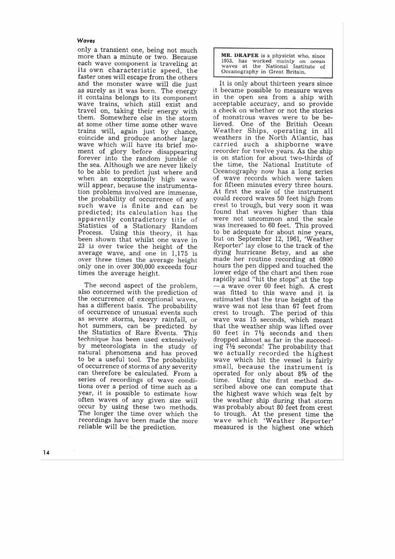


The Glorious Three
Commandant FredericMoreautranslated by Michel Olagnon and G Anderson Chase
IFREMER Centre de BrestBP F Plouzane France
MichelOlagnonifremerfr
WWW home page httpwwwifremerfrmetocean Department of Maritime Transportation
Maine Maritime AcademyCastine ME USA
achasemmaedu
WWW home page httpwwwmainemaritimeedu
Abstract We were given the present note by a former cadet who wenton his roundtheworld cruise in and given its relevance we decided to translate it and publish it together with the Rogue Waves proceedingsA few explanations may be useful as to the context The Glorious Three is the name that was given in French Historyto th th and th of July On th of July King Charles theXth had taken four ordinances The rst two ones suspended freedomof press and the ballot law The other two dissolved the newly electedParliament and organized new elections On th of July workers andpeople of the Paris suburbs started to erect barricades On th theArsenal the Hotel de ville City Hall NotreDame were taken bycrowds following the tricolour ag On th Charles X oered towithdraw the ordinances too late and on th the Duke of Orleanswas appointed by the Parliament King of the French People underthe name of LouisPhilippe
The Jeanne dArc has been for many years the ship on board whichFrench cadets of the Naval Academy sail on their roundtheworldtraining cruise In she was the second of that name and wasonly one year from her last voyage and her replacement by thehelicoptercarrier la Resolue who is currently the third Jeanne dArcand close to her replacement once again When the event occurredthe port propeller shaft had recently broken from fatigue and thepropeller been lost That was no wonder since the ship was built in and had been sailing since
The Jeanne dArc had a displacement of tons and could sail at knots She was armed with double mm turrets mm mm and mm guns She could accomodate cadets inaddition to regular ocers and a crew of

Aboard at sea th of February
Cruiser JEANNE DARC
COMMUNICATION
The morning of th of February was marked by a sea event of short duration less than seconds overall but that nevertheless deserves a few comments tothe intent especially of all those who were submitted to its eects without beingin an appropriate position to observe the cause
To this aim I distribute the attached sheet that briey presents the proceeding of the event as could be observed from the Bridge
Some of you may have wondered could it have made a nasty end It maybe answered to that question
The Jeanne dArc should be able to withstand a heel or so and it didnot quite reach
to roll we would need to face signicantly higher waves and the heightof the Glorious Three to meters was absolutely abnormal sinceeven during a typhoon it is very unusual for a wave to overpass meters
and of course the best way to avoid any risk of sea event is to remain onthe shore
Attention all personnel on board
Commander FREDERICMOREAUExecutive Ocer
NOTE
Be reminded that to heave to means to take such heading and speed asto allow the ship to ride out bad weather conditions the best she can that iswithin acceptable roll and pitch limits
Hoveto course depends on the kind of ship in general the ship shouldhead at an angle between and with the waves direction for the Jeanne
dArc hoveto heading is between and Hoveto speed depends of the waves celerity and of the distance between
two consecutive crests it should always be rather low but still sucient tomaintain rudder eciency Under such conditions the ship who is in additionsubmitted to wind and wave action progresses very slowly and drifts signicantly
Being limited to our starboard propeller makes the ship pay o to port Wewere thus led to heaveto on the port tack ie receiving wind and waves on ourport side so that the action of the propeller would add to that of the rudderand refrain the ship from paying o to starboard under the joint action of windand waves
Had we hoveto on the starboard tack the action of the propeller wouldhave added to that of wind and waves and the rudder would probably not havesuced to avoid the ship falling beam to the sea

Board at sea th of February
Cruiser JEANNE DARC
Object Clearing by the Jeanne dArc of a train of three high waves onth of February
Situation
Ship position at K about nautical miles SouthEast of TokyoWeather very strong westerly galeWind westerly Beaufort to speed to knotsSea westerly swell wave height to metersCourse ship hoveto on the port tack receiving swell from two points on portside ordered course to the helmsman had great diculties to correctyawSpeed Starboard engine rpm the ship had only her starboard propellerline remaining operative Estimated bottom speed knots
Description of the event and of action taken
At about a group of large breaking waves was sighted straight ahead justbeyond an area of relative calm water to meters waveheight
The Captain ordered immediately to the left to make the ship meetthem with a better heading and to protect the propeller
The Jeanne paid o by about degrees allowing her to meet the rst wavetwo points to port The height of that wave has been estimated around meters
It heaved the ship and added to her sway to the left in such a manner thatshe fell into the trough with a signicant trim about and leaning greatlyto starboard heel has been estimated to then she continued paying o forabout twenty degrees
To counter that trend the Captain ordered Helm amidships and then to the right
During the interval of about meters inbetween the rst and the secondwave the Jeanne had time to return approximately to its waterline but she wassoon heeled over to starboard by the second wave until the angle reached about the inclinometer of the safety HQ reached its block at while the shipwas still continuing her rolling motion
During clearance of those two waves the freeboard deck and the quarterdeckwere submerged in turn the sea covered the catwalks of the rst deck water
Approximate position obtained from LORAN Q N G E

reaching the top of the bulkheads at the time of maximum heel The man onwatch at the SILAS buoys that were xed at the height of second deck couldsee the buoys oating one of the oats of the port buoy was torn away
The third wave was cleared in similar conditions but with not as large amplitude motions its height being slightly less than that of the two rst ones
The total duration to clear the three waves was seconds at most
The manoeuver action that was taken has avoided that the ship take thewaves head on which would have raised the risk of serious damage to the Bridgeand upper decks and also of submitting the hull to very high stresses especiallyif the ship had come to ride over the crest of one of the waves
On the other hand the ship rode her way over each of the obstacles glidinginto the troughs and never pounding nor ramming
As a consequence only minor damage was experienced to equipment as wellas to the crew It is noteworthy that all access to the decks had been prohibitedfor more than hours thanks to that no casualty was suered
Remarks
The phenomenon was characterized by abnormal features
The exceptional height of the waves cresttrough height between and meters and their remarkably vertical front
The shortness of the gap between two consecutive waves about one hundredmeters
The travelling direction of the group that came at an angle of twenty tothirty degrees from the main swell
The high velocity of the wave group about knots The shapes of the waves that showed a short crest front to m with
a steep decrease at both ends
Thanks to that extraordinary shape and to their exceptional height thewaves contrasted with the still rough sea and could be detected in just sucienttime to change the ships heading to an appropriate course
It should be noted that the Victor Schlcher which was hoveto abaft the beamat about two nautical miles and saw the Jeanne dArc disappear on three occasions into the troughs did not have to face the wave train

In the absence of other explanation it may be assumed that the wave train arosefrom a resonance between the swell and the wind or more probably betweentwo wave systems one resulting from the wind prevailing before the passage ofthe cold front the other about from the rst created by the wind blowingafter the passage of the front
Fig The Jeanne dArc

Fig The Glorious Three Liberty leading the People painting by EugeneDelacroix


A Possible Freak Wave Event Measured at the Draupner Jacket January 1 1995
Sverre Haver
Marine Structures and Risers, Statoil ASA, N-4035 Stavanger, Norway [email protected]
Abstract. A brief informal description of the weather conditions at the Draupner platform January 1. 1995 is given. During this day a wave with a majestic crest height, often referred to as the New Year Wave or the Draupner Wave, was measured by a down-looking laser. The crest height is clearly an outlier in view of what is expected for that sea state and is considered as a possible freak wave event.
1 Introductory remarks
As a response to a request for some info on this subject during the summer 2003, a brief description of the wave event and the conditions January 1 1995 at the Draupner field is given below. The description has been updated and modified several times during the last year.
The platform in the front (the platform with living quarter) is Draupner S, which
was installed in the mid-eighties, while the aft platform, Draupner E, was installed during the summer 1994. Draupner E is the first platform build with a bucket foundation and in order to verify the bucket loading and bucket behaviour, the platform was instrumented for that purpose during the first winter. The instrumentation involved a down looking laser based wave sensor. The wave sensor is said to be located at a platform corner, Haver and Karunakaran (1998). Presently I do not remember which corner, but it is most likely the northern platform corner. The well-known Draupner wave was measured at the wave sensor on the Draupner E platform, i.e. the unmanned platform. It is seen that the platform is rather transparent, i.e. wave measurements are not likely to be much disturbed by the platform legs.
2 The Weather Situation January 1
The weather situation in the North Sea January 1 at 12UTC is indicated in Fig 1. The weather pattern is dominated by a major low with center in Southern Sweden causing a strong northerly wind field over the whole North Sea and Norwegian Sea. In addition to the major low, a smaller low has been moving southwards in the North Sea during the morning hours and in Fig. 1 it is indicated to be located close to

Skagerak. The effect of this smaller low is to strengthen the wind field in the western North Sea. As the smaller low moved southwards, the area with the strongest wind field moved southwards as indicated in Fig. 2. The wind conditions seemed to peak at hurricane level wind between 12UTC and 18UTC. The Draupner platform is located more or less straight west of the southern tip of Norway midway between Norway and Scotland. This means that the platform was outside the area where the wind conditions seem to have been most extreme.
Fig. 0. The Draupner S and Draupner E platforms in the North Sea,
Photo: Øyvind Hagen, Statoil.
The England – Norway ferry “Color Viking” was hit by this storm event on its way over the North Sea. In an interview, the ship master told he had never experienced such weather during his years as a ship master of Color Line ferries. The bridge of this ferry is about 30m above sea level when floating on even keel. In the same interview the ship master said that in connection with the highest waves, those on the bridge looked upwards on the wave crests approaching the vessel. Although it may be somewhat difficult relate observations to a horizontal base line in this sort of weather conditions due to ship pitching and rolling, the statement clearly suggests that a number of rather extreme wave crests seem to have occurred in a certain area of the storm event.
One interesting aspect of the overall situation is the local enhancement of an
underlying strong wind field by the secondary low moving southwards. It may well be that this will result a significant increase of sea state steepness over certain areas. In

turn this may represent conditions being favourable regarding non-linear wave phenomena.
A more detailed discussion of the weather pattern that particular day can be obtained by contacting e.g. The Norwegian Meteorological Institute in Bergen.
3 Wave Conditions at Draupner
At Draupner the wave conditions started increasing late in morning. The significant wave height reached 11 –12 m just after noon and stayed at that level until early evening, Haver and Andersen (2000). For a significant wave height we will expect the maximum wave height (height from trough to crest) to be about 20, but occasionally it may well be 10-15% higher. The maximum crest height (height from still water level until wave crest) would be expected to be about 15m. We have a number of 20-minute observations of the wave condition during peak level of the storm. Most of these show nothing particular, see e.g. Fig. 3, which is rather representative for most of the 20-min. time histories. (It should be noted that we merely have one 20-min record every hour, i.e. no measurements are made for 2/3 of the time.)
The 20-min. wave history collected at about 15:20, however, did include a very
extreme wave event bearing in mind the sea state conditions. The time history is shown in Fig 4, and a closer look at the extreme wave is given in Fig. 5. The maximum wave height is close to 26m. For the actual area, the wave with an annual probability of 10-2 (i.e. the so-called 100-year wave height) was estimated to be around 27m. This means that the wave height in itself is not that extreme, but we did not expect the wave height to be realized in a sea with a 12m significant wave height. It is more likely to be experienced in a sea state with 13-14m significant wave height.
The wave spectrum for the time history shown in Fig. 4 is shown in Fig.6.
Although the estimated spectral ordinates are associated with a considerable statistical uncertainty, the estimated spectrum clearly suggests the existence of two sea systems. This is in agreement with the previous description of the weather scenario January 1 1995.
The extreme pattern of this wave event is its asymmetry about the still water level.
The crest height reaches about 18.5m above still water level. For the actual area, the crest height occurring with an annual probability of 10-4 (i.e. 10000-year crest height) was at that time estimated to be 19.5m. This means that the crest event was not beyond design parameters, but we did not expect such a wave to occur for a significant wave height of 12m. None of our basic engineering approaches suggest the possibility of such a crest height for a 12m sea state. We think the measured event is of good quality. Of course some uncertainties may be associated with the crest height, but the uncertainties or possible biases cannot bring the wave event into the class of typical (slightly non-Gaussian) wave events. The measured structural loads do also

suggest that a big wave hit the structure, but the loads are relatively speaking not as bad as the observed crest height. Although the crest height is well beyond the 10-2 probability crest height, the maximum platform loads do not exceed that level. This suggests that the shape of the wave do differ from our typical design waves. As the wave passed the structure, it was rather close to a temporary deck and as I remember being told some minor damage was reported to equipment located on that deck. To my knowledge, people onboard the next neighbour platform, see Fig. 0, did not particularly note the wave event as it happened. But of course during those weather conditions nobody will be out on the open deck area. It is said in the platform daily journal that all work on deck was stopped at 15:00 due to very strong wind.
4 Freak waves
A number of people and institutions have been given access to the Draupner time history. I think there is a general agreement that the wave event can be referred to as a freak event, i.e. an event that would not be expected under our typical engineering models for extreme wave predictions. I think there is competing ideas regarding explaining the event and not least regarding modeling it mathematically, but my favourite theory involves self-focusing of energy of a wave group into one majestic wave event, i.e. the big event steal energy from its neighbours. The major challenge from my point of view is to understand when and why this strongly non-linear self-focusing process is turned on.
5 References
Sunde, Alv (1995): “Kjempebølger i Nordsjøen” (Extreme Waves in the North Sea), Paper is written in Norwegian, Vær &Klima, Nr.1, 1995.
Haver, S. and Andersen, O. J. (2000): “ Freak waves – Rare Realizations of a
Typical Population or Typical Realizations of a Rare Population?”, ISOPE’2000, Seattle.
Haver, S. and Karunakaran, D. (1998): “Probabilistic description of crest heights of ocean waves”, Proceedings 5th International Workshop of Wave Hindcasting and Forecasting, Melbourne, Florida, January 1998.
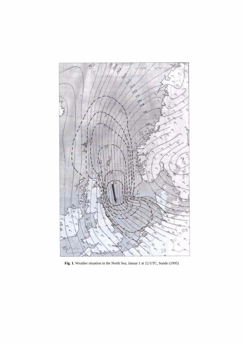
Fig. 1. Weather situation in the North Sea, Januar 1 at 12 UTC, Sunde (1995)

Fig. 2. Area with most severe wind during January 1, Sunde (1995).

Wave Record at 16:20
-10,00
-6,00
-2,00
2,00
6,00
10,00
14,00
0 200 400 600 800 1000 1200
Time (s)
Wav
e el
evat
ion
(m)
Fig. 3. A typical 20-min. time history of surface elevation during the storm.
Draupner wave recordJanuary 1 1995 at 15:20, hs = 11.9m
-8
-4
0
4
8
12
16
20
0 200 400 600 800 1000 1200
Time (s)
Surfa
ce e
leva
tion
(m)
Fig. 4. Time history including an possible freak wave event

Draupner wave recordJanuary 1 1995 at 15:20, hs = 11.9m
-8
-4
0
4
8
12
16
20
180 200 220 240 260 280 300 320 340 360 380
Time (s)
Surfa
ce e
leva
tion
(m)
Fig. 5. A closer look at the possible freak wave event.
Fig. 6. Estimated wave spectrum for the 15:20 wave time history, Haver and
Karunakaran (1998)

Achevé d’imprimer sur les presses de Cloitre Imprimeurs
ISSN 0761-3962 ISBN 2-84433-150-5 ! Dépôt légal 3e trimestre 2005
All rights reserved - © 2005, Ifremer. No part of the material protected by this copyright notice may be reproduced or utilized in any form or by any means,
electronic or mechanical including photocopying, recording, or by any information storage and retrieval system, without written permission from the copyright owner.

Rogue waves 2004 Brest, 20-21-22 October 2004 Since the Rogue Waves 2000 workshop, significant advances have been made in the proposition of models and descriptions that may improve our understanding of rogue waves. Questions arise now on how those results should influence standard practices in the shipbuilding and offshore industries, and whether they allow to impro-ve forecast and warning systems. The Brest Rogue Waves 2004 workshop gathered again many scientists and engineers to an opportunity to confront and discuss their views on the subject. Keywords: ocean waves, extremes, rogue waves, freak waves.
Rogue waves 2004 Brest, 20-21-22 octobre 2004 Depuis le colloque Rogue Waves 2000, des avancées significatives ont été réalisées dans la description et la proposition de modèles susceptibles d’améliorer notre compréhension des vagues scélérates. Les questions qui se posent maintenant concernent l’influence que ces résultats doivent avoir sur les normes et pratiques de la construction navale et offshore, et s'ils apportent des possibilités d'amélioration pour les systèmes de prévision et d’alerte. Le colloque Rogue Waves 2004 de Brest a de nouveau rassemblé de nombreux scientifiques et ingé-nieurs qui ont pu y confronter et discuter leurs positions sur le sujet. Mots-clés : vagues, extrêmes, vagues anormales, vagues scélérates.
Tïwïiwa
39 Éditions Ifremer BP 70, F-29280 Plouzané tel. 33(0)298224013 fax 33 (0)298224586 mél : [email protected]
DIFFUSION : INRA Éditions RD 10, F-78026 Versailles Cedex
VENTE PAR CORRESPONDANCE : tél. 33 (0)1 30 83 34 06 fax 33 (0)1 30 83 34 49 mél : [email protected]
VENTE AUX LIBRAIRES ET ASSIMILÉS : tél. 33 (0)1 30 83 34 01 fax 33 (0)1 30 83 31 58 mél : [email protected]
ISSN 0761-3962 ISBN 2-84433-150-5
35 €
Copyright © 2022 FDOKUMEN