Stock Assessment Form Demersal species - Archimer

Stock Assessment Form

Demersal species HAKE – GSA 7

Reference year: 1998-2015

Reporting year: 2016

[A brief abstract may be added here]

1

Stock Assessment Form version 1.0 (January 2014)

Uploader: Angélique Jadaud*, Beatriz Guijarro**, Enric Massutí*

* IFREMER-UMR MARBEC, 1 rue Jean Monnet, BP 171, 34203 Sète (France); **IEO- Centre Oceanogràfic de

les Balears; Moll de Ponent s/n; 07015 Palma de Mallorca (Spain)

Stock assessment form

1. Basic Identification Data .............................................................................................................. 2

2. Stock identification and biological information ........................................................................... 3

2.1. Stock unit ..................................................................................................................................... 3

2.2. Growth and maturity ................................................................................................................... 3

3. Fisheries information ................................................................................................................... 7

3.1. Description of the fleet ................................................................................................................ 7

3.2. Historical trends ......................................................................................................................... 10

3.3. Management regulations ........................................................................................................... 10

3.4. Reference points ........................................................................................................................ 11

4. Fisheries independent information ........................................................................................... 12

4.1. MEDITS ....................................................................................................................................... 12

4.1.1. Brief description of the direct method used ....................................................................... 12

4.1.2. Spatial distribution of the resources ................................................................................... 13

4.1.3. Historical trends .................................................................................................................. 13

5. Ecological information ............................................................................................................... 15

5.1. Protected species potentially affected by the fisheries ............................................................. 15

5.2. Environmental indexes ............................................................................................................... 15

6. Stock Assessment ....................................................................................................................... 16

6.1. XSA ............................................................................................................................................. 16

6.1.1. Model assumptions ............................................................................................................. 16

6.1.2. Scripts .................................................................................................................................. 16

6.1.3. Input data and Parameters .................................................................................................. 16

6.1.4. Tuning data .......................................................................................................................... 19

6.1.5. Results ................................................................................................................................. 20

6.1.6. Robustness analysis ............................................................................................................. 23

6.1.7. Retrospective analysis. comparison between model runs. sensitivity analysis. etc. .......... 23

6.1.8. Assessment quality .............................................................................................................. 25

6.1.9. Comparison between XSA and a4a ..................................................................................... 25

7. Stock predictions ........................................................................................................................ 26

7.1. Short term predictions 2016-2018 ............................................................................................. 26

7.2. Short term predictions 2015-2017 by fleet ............................................................................... 27

7.2.1. Method ................................................................................................................................ 27

7.2.2. Input parameters ................................................................................................................. 27

7.2.3. Results ................................................................................................................................. 27

7.3. Medium term predictions .......................................................................................................... 28

7.4. Long term predictions ................................................................................................................ 28

8. Draft scientific advice ................................................................................................................. 28

9. Explanation of codes .................................................................................................................. 30

2

1. Basic Identification Data

Scientific name: Common name: ISCAAP Group:

Merluccius merluccius - HKE European hake 32 HKE

1st Geographical sub-area: 2nd Geographical sub-area: 3rd Geographical sub-area:

07 – Gulf of Lions

1st Country 2nd Country 3rd Country

France Spain

Stock assessment method: (direct, indirect, combined, none)

XSA (tuning with MEDITS indices) and Y/R

Authors:

Angélique Jadaud*, Beatriz Guijarro**, Enric Massutí*

Affiliation:

* IFREMER, 1 rue Jean Monnet, BP 171, 34203 Sète (France);

**IEO-Centre Oceanogràfic de les Balears; Moll de Ponent s/n; 07015 Palma de Mallorca (Spain)

The ISSCAAP code is assigned according to the FAO 'International Standard Statistical Classification for

Aquatic Animals and Plants' (ISSCAAP) which divides commercial species into 50 groups on the basis of their

taxonomic, ecological and economic characteristics. This can be provided by the GFCM secretariat if

needed. A list of groups can be found here:

http://www.fao.org/fishery/collection/asfis/en

Direct methods (you can choose more than one):

- Acoustics survey

- Egg production survey

- Trawl survey

- SURBA

- Other (please specify)

Indirect method (you can choose more than one):

- XSA

- A4a

http://www.fao.org/fishery/collection/asfis/en

3

2. Stock identification and biological information

2.1. Stock unit

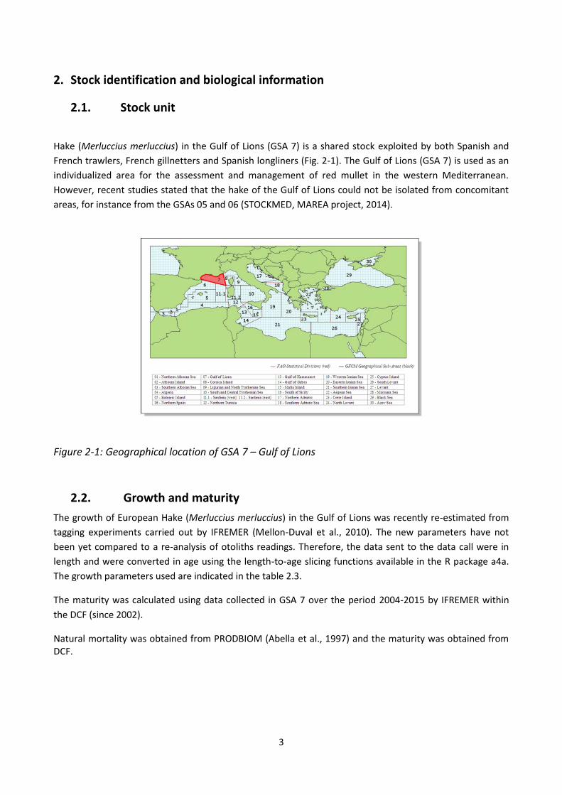
Hake (Merluccius merluccius) in the Gulf of Lions (GSA 7) is a shared stock exploited by both Spanish and

French trawlers, French gillnetters and Spanish longliners (Fig. 2-1). The Gulf of Lions (GSA 7) is used as an

individualized area for the assessment and management of red mullet in the western Mediterranean.

However, recent studies stated that the hake of the Gulf of Lions could not be isolated from concomitant

areas, for instance from the GSAs 05 and 06 (STOCKMED, MAREA project, 2014).

Figure 2-1: Geographical location of GSA 7 – Gulf of Lions

2.2. Growth and maturity

The growth of European Hake (Merluccius merluccius) in the Gulf of Lions was recently re-estimated from

tagging experiments carried out by IFREMER (Mellon-Duval et al., 2010). The new parameters have not

been yet compared to a re-analysis of otoliths readings. Therefore, the data sent to the data call were in

length and were converted in age using the length-to-age slicing functions available in the R package a4a.

The growth parameters used are indicated in the table 2.3.

The maturity was calculated using data collected in GSA 7 over the period 2004-2015 by IFREMER within

the DCF (since 2002).

Natural mortality was obtained from PRODBIOM (Abella et al., 1997) and the maturity was obtained from DCF.

4

Table 2.2.2-1: Maximum size, size at first maturity and size at recruitment.

Somatic magnitude measured

(LT, LC, etc) Units centimeters

Sex

Fem Mal Combined

Reproduction

season

All year with higher picks of

spawning at the beginning of

spring and end of automn (Oliver,

1991), with a lot of fluctuations

from one year to another

(Recasens, 1992)

Maximum

size

observed

96 57 96

Recruitment

season

All year (higher picks in winter and

spring)

Size at first

maturity 29

Spawning area Shelf & upper slope

Recruitment

size to the

fishery

5

Nursery area Shelf

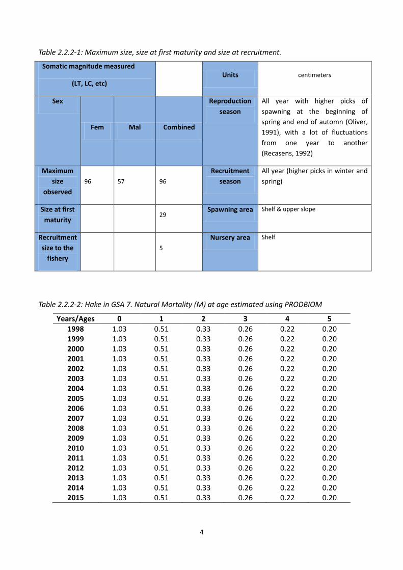
Table 2.2.2-2: Hake in GSA 7. Natural Mortality (M) at age estimated using PRODBIOM

Years/Ages 0 1 2 3 4 5

1998 1.03 0.51 0.33 0.26 0.22 0.20 1999 1.03 0.51 0.33 0.26 0.22 0.20 2000 1.03 0.51 0.33 0.26 0.22 0.20 2001 1.03 0.51 0.33 0.26 0.22 0.20 2002 1.03 0.51 0.33 0.26 0.22 0.20 2003 1.03 0.51 0.33 0.26 0.22 0.20 2004 1.03 0.51 0.33 0.26 0.22 0.20 2005 1.03 0.51 0.33 0.26 0.22 0.20 2006 1.03 0.51 0.33 0.26 0.22 0.20 2007 1.03 0.51 0.33 0.26 0.22 0.20 2008 1.03 0.51 0.33 0.26 0.22 0.20 2009 1.03 0.51 0.33 0.26 0.22 0.20 2010 1.03 0.51 0.33 0.26 0.22 0.20 2011 1.03 0.51 0.33 0.26 0.22 0.20 2012 1.03 0.51 0.33 0.26 0.22 0.20 2013 1.03 0.51 0.33 0.26 0.22 0.20 2014 1.03 0.51 0.33 0.26 0.22 0.20 2015 1.03 0.51 0.33 0.26 0.22 0.20

5

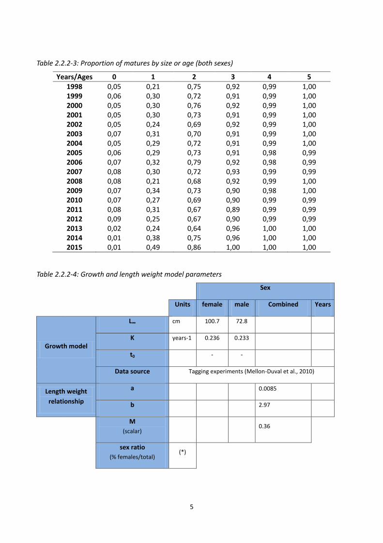
Table 2.2.2-3: Proportion of matures by size or age (both sexes)


1998 0,05 0,21 0,75 0,92 0,99 1,00 1999 0,06 0,30 0,72 0,91 0,99 1,00 2000 0,05 0,30 0,76 0,92 0,99 1,00 2001 0,05 0,30 0,73 0,91 0,99 1,00 2002 0,05 0,24 0,69 0,92 0,99 1,00 2003 0,07 0,31 0,70 0,91 0,99 1,00 2004 0,05 0,29 0,72 0,91 0,99 1,00 2005 0,06 0,29 0,73 0,91 0,98 0,99 2006 0,07 0,32 0,79 0,92 0,98 0,99 2007 0,08 0,30 0,72 0,93 0,99 0,99 2008 0,08 0,21 0,68 0,92 0,99 1,00 2009 0,07 0,34 0,73 0,90 0,98 1,00 2010 0,07 0,27 0,69 0,90 0,99 0,99 2011 0,08 0,31 0,67 0,89 0,99 0,99 2012 0,09 0,25 0,67 0,90 0,99 0,99 2013 0,02 0,24 0,64 0,96 1,00 1,00 2014 0,01 0,38 0,75 0,96 1,00 1,00 2015 0,01 0,49 0,86 1,00 1,00 1,00

Table 2.2.2-4: Growth and length weight model parameters

Sex

Units female male Combined Years

Growth model

L∞ cm 100.7 72.8

K years-1 0.236 0.233

t0 - -

Data source Tagging experiments (Mellon-Duval et al., 2010)

Length weight

relationship

a 0.0085

b 2.97

M

(scalar) 0.36

sex ratio

(% females/total) (*)

6

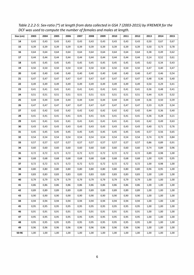
Table 2.2.2-5: Sex-ratio (*) at length from data collected in GSA 7 (2003-2015) by IFREMER for the DCF was used to compute the number of females and males at length.

Size (cm) 2003 2004 2005 2006 2007 2008 2009 2010 2011 2012 2013 2014 2015

14 0,43 0,43 0,43 0,43 0,43 0,43 0,43 0,43 0,43 0,43 0,50 0,67 0,67

15 0,39 0,39 0,39 0,39 0,39 0,39 0,39 0,39 0,39 0,39 0,50 0,73 0,78

16 0,64 0,64 0,64 0,64 0,64 0,64 0,64 0,64 0,64 0,64 0,38 0,49 0,62

17 0,44 0,44 0,44 0,44 0,44 0,44 0,44 0,44 0,44 0,44 0,14 0,52 0,61

18 0,45 0,45 0,45 0,45 0,45 0,45 0,45 0,45 0,45 0,45 0,62 0,34 0,43

19 0,50 0,50 0,50 0,50 0,50 0,50 0,50 0,50 0,50 0,50 0,47 0,40 0,47

20 0,40 0,40 0,40 0,40 0,40 0,40 0,40 0,40 0,40 0,40 0,47 0,46 0,54

21 0,47 0,47 0,47 0,47 0,47 0,47 0,47 0,47 0,47 0,47 0,48 0,36 0,40

22 0,49 0,49 0,49 0,49 0,49 0,49 0,49 0,49 0,49 0,49 0,54 0,29 0,41

23 0,41 0,41 0,41 0,41 0,41 0,41 0,41 0,41 0,41 0,41 0,36 0,48 0,41

24 0,51 0,51 0,51 0,51 0,51 0,51 0,51 0,51 0,51 0,51 0,44 0,35 0,32

25 0,44 0,44 0,44 0,44 0,44 0,44 0,44 0,44 0,44 0,44 0,36 0,50 0,39

26 0,47 0,47 0,47 0,47 0,47 0,47 0,47 0,47 0,47 0,47 0,33 0,29 0,34

27 0,42 0,42 0,42 0,42 0,42 0,42 0,42 0,42 0,42 0,42 0,44 0,36 0,40

28 0,41 0,41 0,41 0,41 0,41 0,41 0,41 0,41 0,41 0,41 0,36 0,28 0,21

29 0,41 0,41 0,41 0,41 0,41 0,41 0,41 0,41 0,41 0,41 0,42 0,49 0,63

30 0,43 0,43 0,43 0,43 0,43 0,43 0,43 0,43 0,43 0,43 0,40 0,71 0,76

31 0,45 0,45 0,45 0,45 0,45 0,45 0,45 0,45 0,45 0,45 0,57 0,56 0,65

32 0,54 0,54 0,54 0,54 0,54 0,54 0,54 0,54 0,54 0,54 0,74 0,70 0,84

33 0,57 0,57 0,57 0,57 0,57 0,57 0,57 0,57 0,57 0,57 0,86 0,89 0,91

34 0,60 0,60 0,60 0,60 0,60 0,60 0,60 0,60 0,60 0,60 0,74 0,89 0,96

35 0,72 0,72 0,72 0,72 0,72 0,72 0,72 0,72 0,72 0,72 0,89 0,98 1,00

36 0,68 0,68 0,68 0,68 0,68 0,68 0,68 0,68 0,68 0,68 1,00 0,95 0,95

37 0,72 0,72 0,72 0,72 0,72 0,72 0,72 0,72 0,72 0,72 1,00 0,98 1,00

38 0,80 0,80 0,80 0,80 0,80 0,80 0,80 0,80 0,80 0,80 0,96 0,95 1,00

39 0,83 0,83 0,83 0,83 0,83 0,83 0,83 0,83 0,83 0,83 1,00 1,00 1,00

40 0,79 0,79 0,79 0,79 0,79 0,79 0,79 0,79 0,79 0,79 1,00 1,00 1,00

41 0,86 0,86 0,86 0,86 0,86 0,86 0,86 0,86 0,86 0,86 1,00 1,00 1,00

42 0,89 0,89 0,89 0,89 0,89 0,89 0,89 0,89 0,89 0,89 1,00 1,00 1,00

43 0,90 0,90 0,90 0,90 0,90 0,90 0,90 0,90 0,90 0,90 1,00 1,00 1,00

44 0,94 0,94 0,94 0,94 0,94 0,94 0,94 0,94 0,94 0,94 1,00 1,00 1,00

45 0,95 0,95 0,95 0,95 0,95 0,95 0,95 0,95 0,95 0,95 1,00 1,00 1,00

46 0,91 0,91 0,91 0,91 0,91 0,91 0,91 0,91 0,91 0,91 1,00 1,00 1,00

47 0,95 0,95 0,95 0,95 0,95 0,95 0,95 0,95 0,95 0,95 1,00 1,00 1,00

48 0,95 0,95 0,95 0,95 0,95 0,95 0,95 0,95 0,95 0,95 1,00 1,00 1,00

49 0,96 0,96 0,96 0,96 0,96 0,96 0,96 0,96 0,96 0,96 1,00 1,00 1,00

50-96 1,00 1,00 1,00 1,00 1,00 1,00 1,00 1,00 1,00 1,00 1,00 1,00 1,00

7

3. Fisheries information

3.1. Description of the fleet

Hake is one of the most important demersal target species for the commercial fisheries in the Gulf of Lions

(GSA 7). In this area, hake is exploited by French trawlers, French gillnetters, Spanish trawlers and Spanish

longliners. Since 1998, an average of 243 boats are involved in this fishery and, according to official

statistics, the total annual catches for the period 1998-2015 have oscillated around an average value of

1961 tons (1139 tons in 2015). In 2009, because of the large decline of small pelagic fish species in the area,

the trawlers fishing small pelagic have diverted their effort on demersal species. Between 1998 and 2015,

the number of French trawlers operating in the GSA 07 has decreased by 50%. The French trawler fleet is

the largest considering catches realized, the proportion of boats and catches are respectively (27% and

73%). The length of hake in the trawler catches ranges between 3 and 92 cm total length (TL), with an

average size of 21 cm TL. The second largest fleet is the French gillnetters (41 and 16% respectively, range

13-86 cm TL and average size 39 cm TL), followed by the Spanish trawlers (9 and 10%, respectively, range 5-

88 cm TL, and average size 24 cm TL), and the Spanish longliners (4 and 1%, respectively, range 22-96 cm TL

and average size 52 cm TL). The hake trawlers exploit a highly diversified species assemblage: Striped red

mullet (Mullus surmuletus), red mullet (M. barbatus), angler fish (L. piscatorius), blackbellied angler fish (L.

budegassa), european conger (Conger conger), poor-cod (Trisopterus minutus capelanus), fourspotted

megrim (Lepidorhombus boscii), soles (Solea spp.), horned octopus (Eledone cirrhosa), squids (Illex

coindetii), gilthead seabream (Sparus aurata), European seabass (Dicentrarchus labrax), seabreams

(Pagellus spp.), blue whiting (Micromesistius poutassou), tub gurnard (Chelidonichtys lucerna).

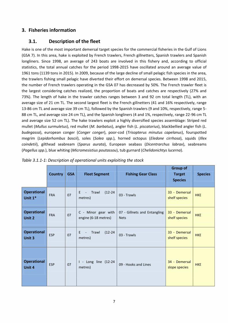
Table 3.1.1-1: Description of operational units exploiting the stock

Country GSA Fleet Segment Fishing Gear Class

Group of

Target

Species

Species

Operational

Unit 1* FRA 07

E - Trawl (12-24

metres) 03 - Trawls

33 - Demersal

shelf species HKE

Operational

Unit 2 FRA 07

C - Minor gear with

engine (6-18 metres)

07 - Gillnets and Entangling

Nets

33 - Demersal

shelf species HKE

Operational

Unit 3 ESP 07

E - Trawl (12-24

metres) 03 - Trawls

33 - Demersal

shelf species HKE

Operational

Unit 4 ESP 07

I - Long line (12-24

metres) 09 - Hooks and Lines

34 - Demersal

slope species HKE

8

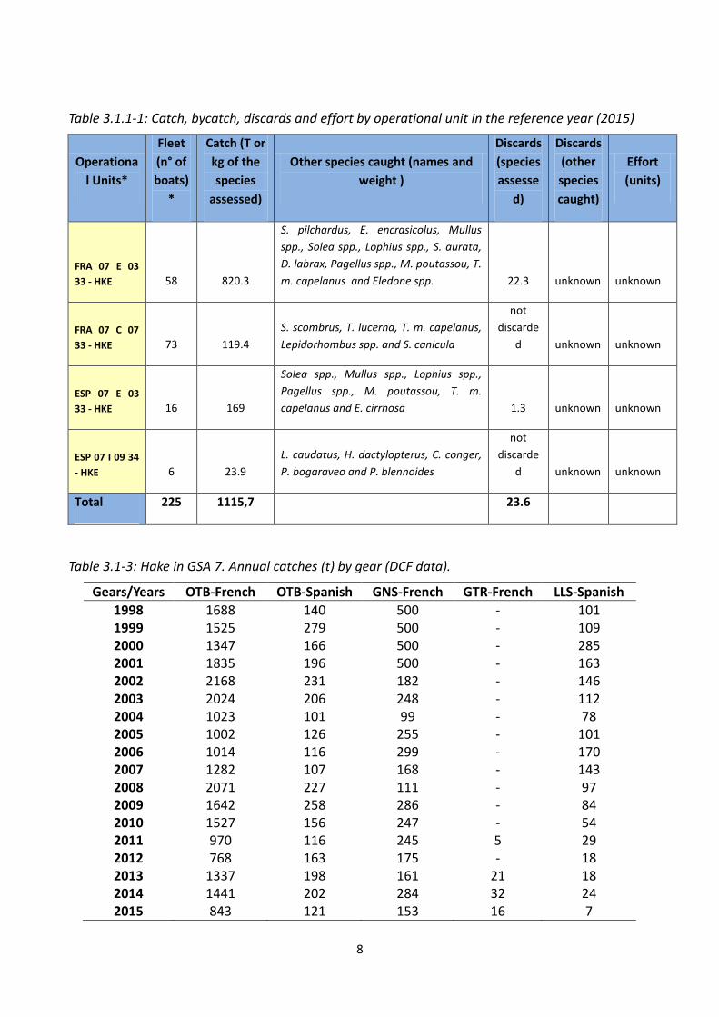
Table 3.1.1-1: Catch, bycatch, discards and effort by operational unit in the reference year (2015)

Operationa

l Units*

Fleet

(n° of

boats)

*

Catch (T or

kg of the

species

assessed)

Other species caught (names and

weight )

Discards

(species

assesse

d)

Discards

(other

species

caught)

Effort

(units)

FRA 07 E 03

33 - HKE 58 820.3

S. pilchardus, E. encrasicolus, Mullus

spp., Solea spp., Lophius spp., S. aurata,

D. labrax, Pagellus spp., M. poutassou, T.

m. capelanus and Eledone spp. 22.3 unknown unknown

FRA 07 C 07

33 - HKE 73 119.4

S. scombrus, T. lucerna, T. m. capelanus,

Lepidorhombus spp. and S. canicula

not

discarde

d unknown unknown

ESP 07 E 03

33 - HKE 16 169

Solea spp., Mullus spp., Lophius spp.,

Pagellus spp., M. poutassou, T. m.

capelanus and E. cirrhosa 1.3 unknown unknown

ESP 07 I 09 34

- HKE 6 23.9

L. caudatus, H. dactylopterus, C. conger,

P. bogaraveo and P. blennoides

not

discarde

d unknown unknown

Total 225 1115,7 23.6

Table 3.1-3: Hake in GSA 7. Annual catches (t) by gear (DCF data).

Gears/Years OTB-French OTB-Spanish GNS-French GTR-French LLS-Spanish

1998 1688 140 500 - 101 1999 1525 279 500 - 109 2000 1347 166 500 - 285 2001 1835 196 500 - 163 2002 2168 231 182 - 146 2003 2024 206 248 - 112 2004 1023 101 99 - 78 2005 1002 126 255 - 101 2006 1014 116 299 - 170 2007 1282 107 168 - 143 2008 2071 227 111 - 97 2009 1642 258 286 - 84 2010 1527 156 247 - 54 2011 970 116 245 5 29 2012 768 163 175 - 18 2013 1337 198 161 21 18 2014 1441 202 284 32 24 2015 843 121 153 16 7

9

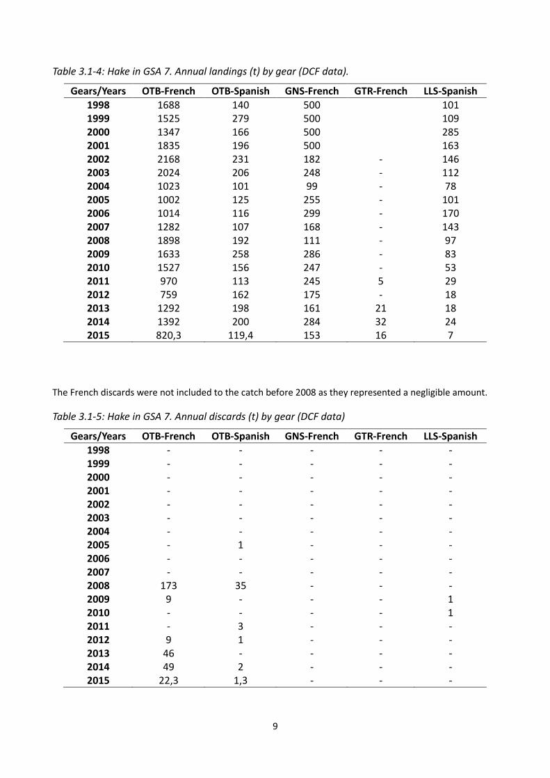
Table 3.1-4: Hake in GSA 7. Annual landings (t) by gear (DCF data).


1998 1688 140 500

101 1999 1525 279 500

109

2000 1347 166 500

285 2001 1835 196 500

163

2002 2168 231 182 - 146 2003 2024 206 248 - 112 2004 1023 101 99 - 78 2005 1002 125 255 - 101 2006 1014 116 299 - 170 2007 1282 107 168 - 143 2008 1898 192 111 - 97 2009 1633 258 286 - 83 2010 1527 156 247 - 53 2011 970 113 245 5 29 2012 759 162 175 - 18 2013 1292 198 161 21 18 2014 1392 200 284 32 24 2015 820,3 119,4 153 16 7

The French discards were not included to the catch before 2008 as they represented a negligible amount.

Table 3.1-5: Hake in GSA 7. Annual discards (t) by gear (DCF data)


1998 - - - - - 1999 - - - - - 2000 - - - - - 2001 - - - - - 2002 - - - - - 2003 - - - - - 2004 - - - - - 2005 - 1 - - - 2006 - - - - - 2007 - - - - - 2008 173 35 - - - 2009 9 - - - 1 2010 - - - - 1 2011 - 3 - - - 2012 9 1 - - - 2013 46 - - - - 2014 49 2 - - - 2015 22,3 1,3 - - -

10

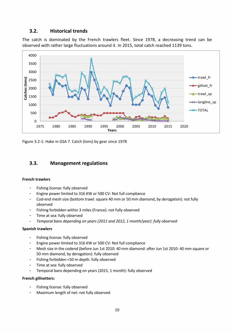
3.2. Historical trends

The catch is dominated by the French trawlers fleet. Since 1978, a decreasing trend can be observed with rather large fluctuations around it. In 2015, total catch reached 1139 tons.

Figure 3.2-1: Hake in GSA 7. Catch (tons) by gear since 1978

3.3. Management regulations

French trawlers

- Fishing license: fully observed

- Engine power limited to 316 KW or 500 CV: Not full compliance

- Cod-end mesh size (bottom trawl: square 40 mm or 50 mm diamond, by derogation): not fully observed

- Fishing forbidden within 3 miles (France): not fully observed

- Time at sea: fully observed

- Temporal bans depending on years (2011 and 2012, 1 month/year): fully observed

Spanish trawlers


- Engine power limited to 316 KW or 500 CV: Not full compliance

- Mesh size in the codend (before Jun 1st 2010: 40 mm diamond: after Jun 1st 2010: 40 mm square or 50 mm diamond, by derogation): fully observed

- Fishing forbidden <50 m depth: fully observed

- Time at sea: fully observed

- Temporal bans depending on years (2015, 1 month): fully observed

French gillnetters:


- Maximum length of net: not fully observed

0

500

1000

1500

2000

2500

3000

3500

4000

1975 1980 1985 1990 1995 2000 2005 2010 2015 2020

Cat

che

s (t

on

s)

Years

trawl_fr

gillnet_fr

trawl_sp

longline_sp

TOTAL

11

Spanish longliners:


- Number of hook per boat: not fully observed

In 2009, GFCM proposed the creation of a High Sea Fishery Restricted Area (FRA, GFCM/33/2009/1) in

which the fishing effort for demersal stocks of vessels using towed nets, bottom and mid-water longlines,

bottom-set nets shall not exceed the level of fishing effort applied in 2008 in the fisheries restricted area of

the eastern Gulf of Lions as bounded by lines joining the following geographic coordinates: 42°40'N, 4°20' E;

42°40'N, 5°00' E; 43°00'N, 4°20' E; 43°00'N, 5°00' E. In the article 4 from the EU Regulation No. 1343/2011

of the European Parliament and of the Council of 13 December 2011, this fisheries restricted area was

established and in 2012 both French (Arrêté du 28 décembre 2012, NOR: TRAM1240493A) and Spanish

(Orden AAA/1857/2012 de 22 de Agosto) governments published their own laws regulating this FRA.

Moreover an important decrease in capacity of French trawler fleet since 2011, reducing the number of

boats by 39% since the beginning of the series (1998).

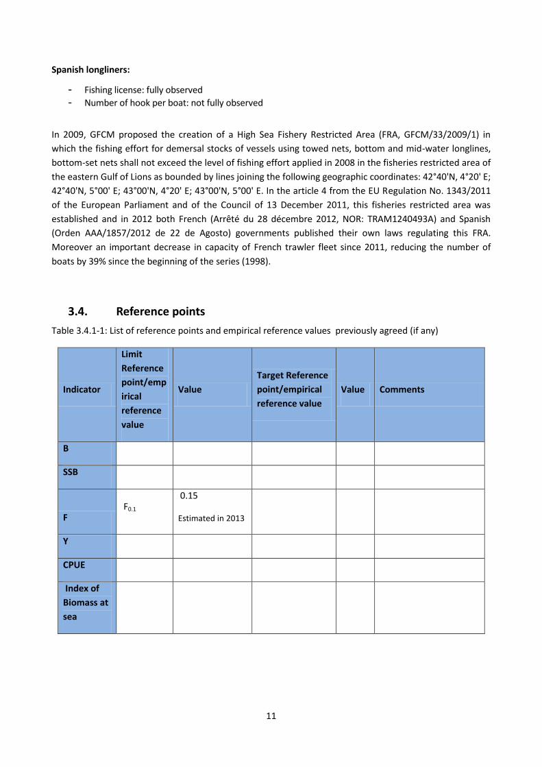
3.4. Reference points

Table 3.4.1-1: List of reference points and empirical reference values previously agreed (if any)

Indicator

Limit

Reference

point/emp

irical

reference

value

Value

Target Reference

point/empirical

reference value

Value Comments

B

SSB

F F0.1

0.15

Estimated in 2013

Y

CPUE

Index of

Biomass at

sea

12

4. Fisheries independent information

4.1. MEDITS

4.1.1. Brief description of the direct method used

Fishery independent information regarding the state of the hake in GSA 7 was derived from the

international survey MEDITS. MEDITS surveys have been carried out from late spring to middle summer,

between 1994 and 2013, following random depth-stratified sampling design. Five depth strata were

considered: 10-49 m, 50-99 m, 100-199 m, 200-499 m and 500-800 m. The gear used was a GOC 73, an

experimental bottom trawl gear, with a cod-end mesh size of 20 mm. Sampling duration depended on the

depth of the sampling station: 30 minutes for the samples on the shelf (10-199 m) and 60 minutes for those

in the slope (200-800 m). See Bertrand et al. (2002) for further details.

The data was assigned to strata based upon the shooting position and average depth (between shooting

and hauling depth). Catches by haul were standardized to 60 minutes hauling duration. The abundance and

biomass indices by GSA were calculated through stratified means (Cochran, 1953; Saville, 1977). This

involves weighting the average values of the individual standardized catches and the variation of each

stratum by the respective stratum areas in each GSA:

Yst = Σ (Yi*Ai) / A

V(Yst) = Σ (Ai² * si ² / ni) / A²

Where: A=total survey area

Ai=area of the i-th stratum

si=standard deviation of the i-th stratum

ni=number of valid hauls of the i-th stratum

n=number of hauls in the GSA

Yi=mean of the i-th stratum

Yst=stratified mean abundance

V(Yst)=variance of the stratified mean

The variation of the stratified mean is then expressed as the 95 % confidence interval:

Confidence interval = Yst ± t(student distribution) * V(Yst) / n

Length distributions were obtained by the sum of all standardized length frequencies (subsamples raised to standardized haul abundance per hour) over the stations of each stratum. Aggregated length frequencies were then raised to stratum abundance * 100 (because of low numbers in most strata) and finally aggregated (sum) over the GSA strata.

13

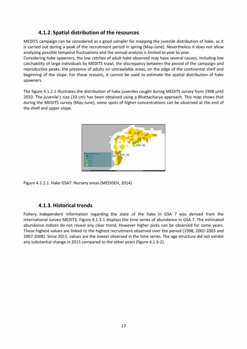
4.1.2. Spatial distribution of the resources

MEDITS campaign can be considered as a good sampler for mapping the juvenile distribution of hake, as it is carried out during a peak of the recruitment period in spring (May-June). Nevertheless it does not allow analyzing possible temporal fluctuations and the annual analysis is limited to year to year. Considering hake spawners, the low catches of adult hake observed may have several causes, including low catchability of large individuals by MEDITS trawl, the discrepancy between the period of the campaign and reproductive peaks, the presence of adults on untrawlable areas, on the edge of the continental shelf and beginning of the slope. For those reasons, it cannot be used to estimate the spatial distribution of hake spawners. The figure 4.1.2.1 illustrates the distribution of hake juveniles caught during MEDITS survey from 1998 until 2010. The juvenile’s size (10 cm) has been obtained using a Bhattacharya approach. This map shows that during the MEDITS survey (May-June), some spots of higher concentrations can be observed at the end of the shelf and upper slope.

Figure 4.1.2.1. Hake GSA7: Nursery areas (MEDISEH, 2014)

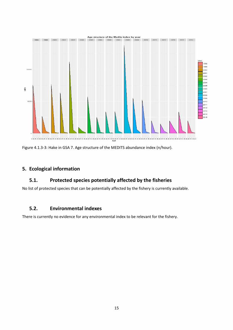
4.1.3. Historical trends

Fishery independent information regarding the state of the hake in GSA 7 was derived from the international survey MEDITS. Figure 4.1.3-1 displays the time series of abundance in GSA 7. The estimated abundance indices do not reveal any clear trend. However higher picks can be observed for some years. These highest values are linked to the highest recruitment observed over the period (1998, 2002-2003 and 2007-2008). Since 2011, values are the lowest observed in the time series. The age structure did not exhibit any substantial change in 2015 compared to the other years (figure 4.1.3-2).

14

Figure 4.1.3-1: Hake in GSA 7. MEDITS abundance index (n/hour).

Figure 4.1.3-2: Hake in GSA 7. Size structure of the MEDITS abundance index (n/hour).

0

500

1000

1500

2000

2500

3000

3500

0 10 20 30 40 50 60

Nu

mb

ers

/ho

ur

Size (cm)

1998

1999

2000

2001

2002

2003

2004

2005

2006

2007

2008

2009

2010

2011

2012

2013

2014

2015

15

Figure 4.1.3-3: Hake in GSA 7. Age structure of the MEDITS abundance index (n/hour).

5. Ecological information

5.1. Protected species potentially affected by the fisheries

No list of protected species that can be potentially affected by the fishery is currently available.

5.2. Environmental indexes

There is currently no evidence for any environmental index to be relevant for the fishery.

16

6. Stock Assessment

6.1. XSA

6.1.1. Model assumptions

The stock assessment was performed over the period 1998-2015 using an XSA model over age classes

ranging from 0 to 5+ and with MEDITS index, as tuning fleet (ages 0-2). The a4a model, developed by the

Joint Research Center, was also used to model the stock (a4a is a statistical catch at age model, whose

flexibility allows to fit a wide range of models to the data). However, the final diagnosis is based upon XSA

analysis, as the population parameters obtained from XSA were considered as more precautionary than

those from a4a. A comparison between the results obtained with both methods can be found in the section

6.1.9.

6.1.2. Scripts

The R script and the data used to perform the final XSA run have been provided to the GFCM.

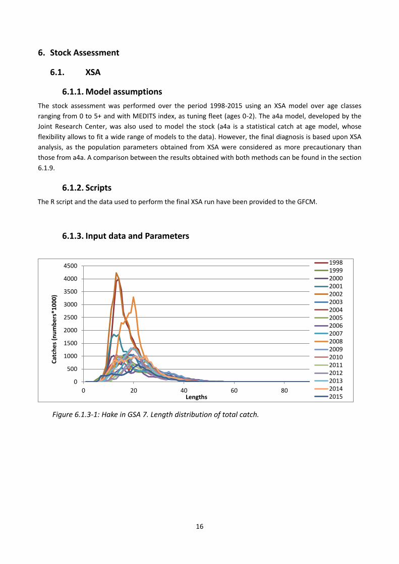
6.1.3. Input data and Parameters

Figure 6.1.3-1: Hake in GSA 7. Length distribution of total catch.

0

500

1000

1500

2000

2500

3000

3500

4000

4500

0 20 40 60 80

Cat

che

s (n

um

be

rs*1

00

0)

Lengths

199819992000200120022003200420052006200720082009201020112012201320142015

17

Figure 6.1.3-1: Hake in GSA 7. Age distribution of total catch.

Table 6.1.3-1: Hake in GSA 7. Catch at age in numbers in thousands (discards included).


1998 20379 13573 1792 233 43 25 1999 6260 8929 2989 303 37 15

2000 7263 6929 2411 349 67 42

2001 12090 9813 2994 374 39 32

2002 23572 14631 2304 271 30 19

2003 5770 10244 3016 376 33 20

2004 5999 5275 1488 173 15 4

2005 5637 5631 1794 193 20 4

2006 2615 4363 1860 277 35 8

2007 2996 6036 2050 268 30 9

2008 10792 18011 1768 166 20 7

2009 3545 7524 2927 388 21 5

2010 6723 9860 2240 216 16 2

2011 2398 6208 1655 169 7 1

2012 2442 6875 1061 104 8 1

2013 5689 10705 1700 19 4 1

2014 6606 10276 2131 28 2 1

2015 3394 5616 1073 18 2 0

0

5000

10000

15000

20000

25000

0 1 2 3 4 5

Cat

che

s (N

um

be

rs*1

00

0)

Ages

199819992000200120022003200420052006200720082009201020112012201320142015

18

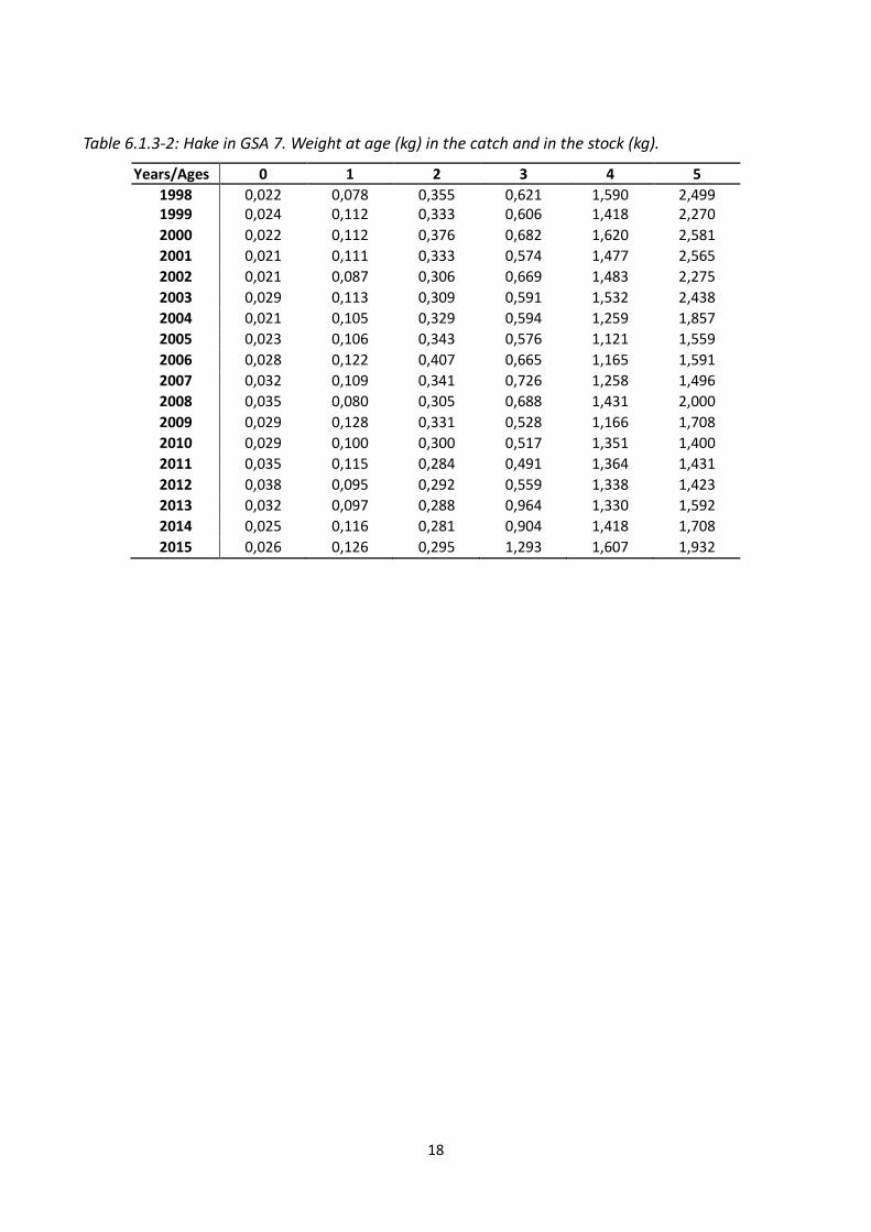
Table 6.1.3-2: Hake in GSA 7. Weight at age (kg) in the catch and in the stock (kg).


1998 0,022 0,078 0,355 0,621 1,590 2,499 1999 0,024 0,112 0,333 0,606 1,418 2,270 2000 0,022 0,112 0,376 0,682 1,620 2,581 2001 0,021 0,111 0,333 0,574 1,477 2,565 2002 0,021 0,087 0,306 0,669 1,483 2,275 2003 0,029 0,113 0,309 0,591 1,532 2,438 2004 0,021 0,105 0,329 0,594 1,259 1,857 2005 0,023 0,106 0,343 0,576 1,121 1,559 2006 0,028 0,122 0,407 0,665 1,165 1,591 2007 0,032 0,109 0,341 0,726 1,258 1,496 2008 0,035 0,080 0,305 0,688 1,431 2,000 2009 0,029 0,128 0,331 0,528 1,166 1,708 2010 0,029 0,100 0,300 0,517 1,351 1,400 2011 0,035 0,115 0,284 0,491 1,364 1,431 2012 0,038 0,095 0,292 0,559 1,338 1,423 2013 0,032 0,097 0,288 0,964 1,330 1,592 2014 0,025 0,116 0,281 0,904 1,418 1,708 2015 0,026 0,126 0,295 1,293 1,607 1,932

19

6.1.4. Tuning data

Table 6.1.4-1: Hake in GSA 7. Catch in numbers (thousands) obtained from MEDITS survey.

Table 6.1.4-1: Hake in GSA 7. MEDITS index at age (1998-2015).

Years/Ages 0 1 2

1998 7534 854 23 1999 2639 341 63

2000 7626 124 48

2001 6276 188 50

2002 11168 557 46

2003 945 357 93

2004 5697 136 28

2005 2468 153 25

2006 3355 92 36

2007 3390 333 63

2008 13728 2177 51

2009 5470 582 118

2010 5218 251 44

2011 1945 163 37

2012 1427 351 16

2013 1915 905 62

2014 3329 426 91

2015 1939 203 26

0

2000

4000

6000

8000

10000

12000

14000

16000

0 1 2 3

Nu

mb

ers

(*1

00

0)

Ages

1998

1999

2000

2001

2002

2003

2004

2005

2006

2007

2008

2009

2010

2011

2012

2013

2014

2015

20

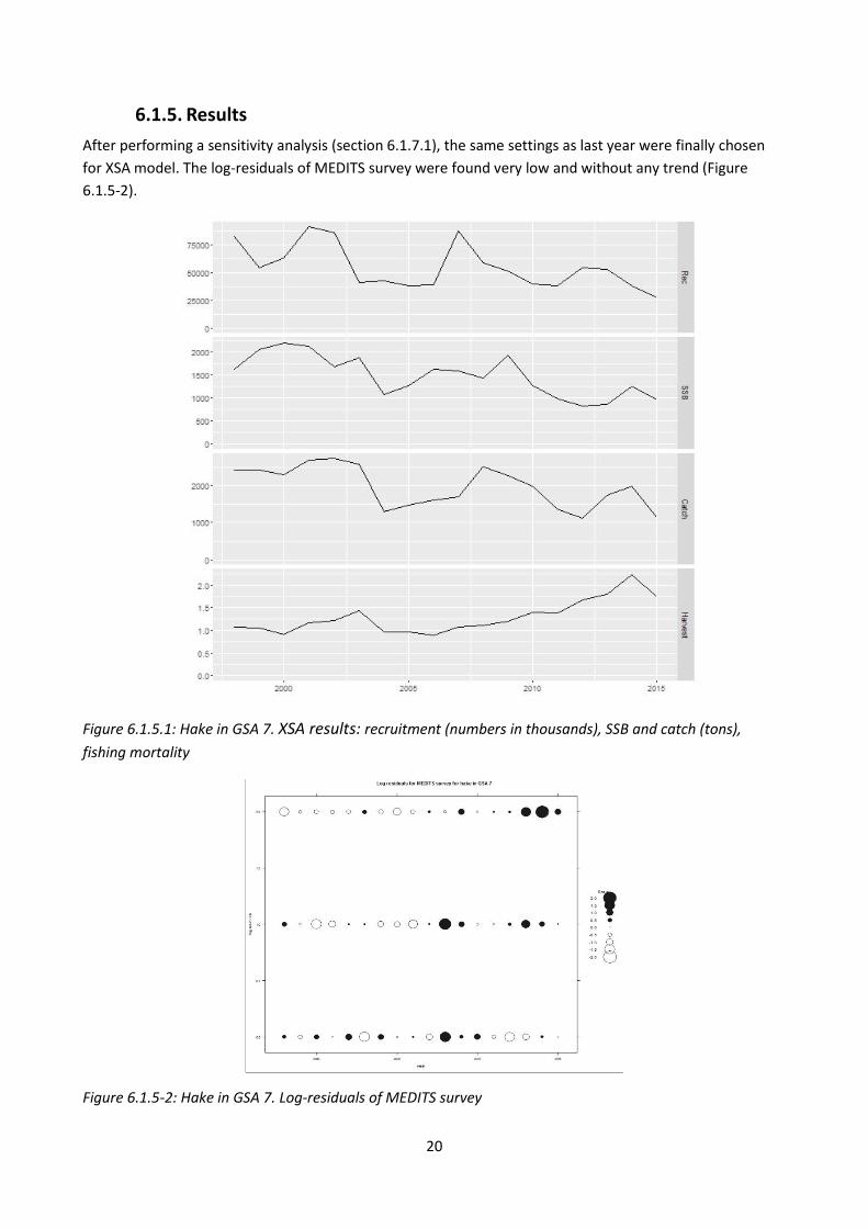
6.1.5. Results

After performing a sensitivity analysis (section 6.1.7.1), the same settings as last year were finally chosen

for XSA model. The log-residuals of MEDITS survey were found very low and without any trend (Figure

6.1.5-2).

Figure 6.1.5.1: Hake in GSA 7. XSA results: recruitment (numbers in thousands), SSB and catch (tons),

fishing mortality

Figure 6.1.5-2: Hake in GSA 7. Log-residuals of MEDITS survey

21

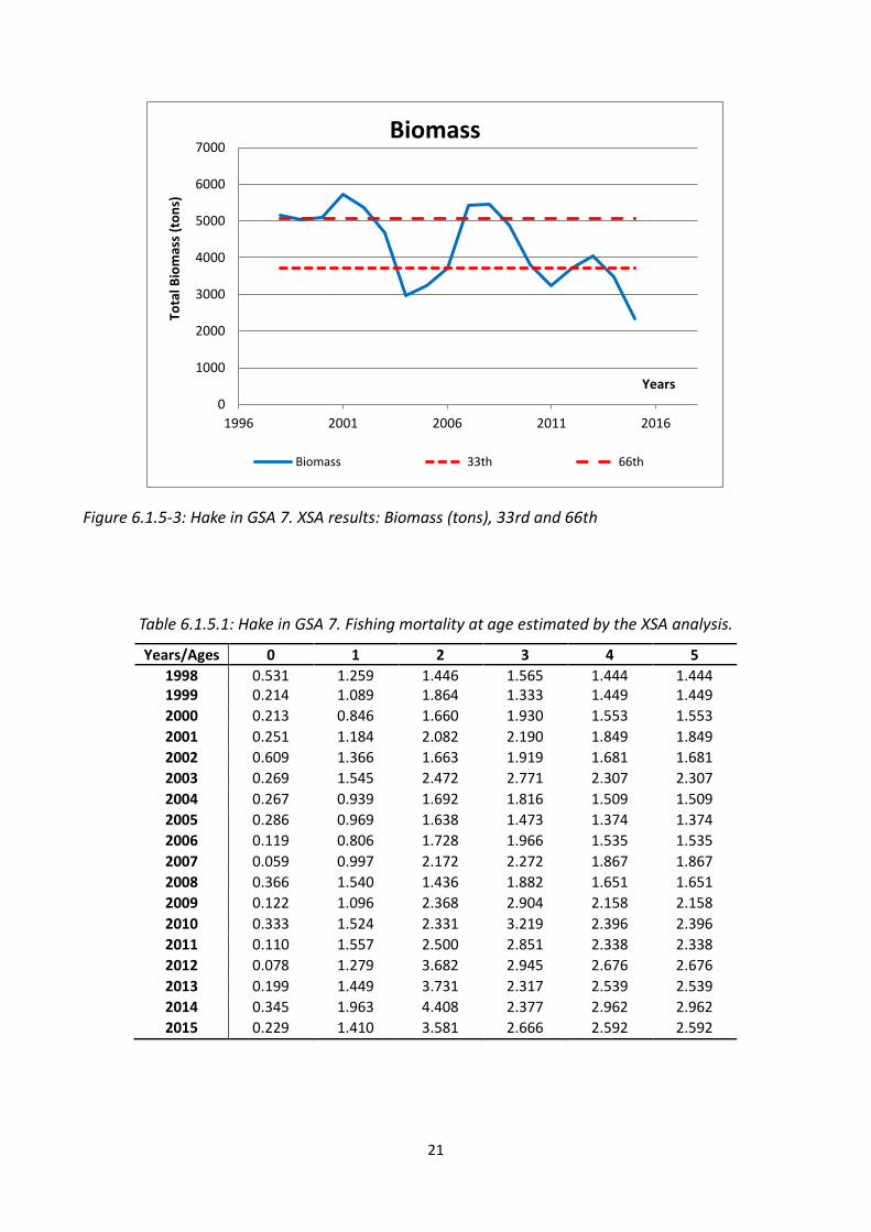
Figure 6.1.5-3: Hake in GSA 7. XSA results: Biomass (tons), 33rd and 66th

Table 6.1.5.1: Hake in GSA 7. Fishing mortality at age estimated by the XSA analysis.


1998 0.531 1.259 1.446 1.565 1.444 1.444 1999 0.214 1.089 1.864 1.333 1.449 1.449

2000 0.213 0.846 1.660 1.930 1.553 1.553

2001 0.251 1.184 2.082 2.190 1.849 1.849

2002 0.609 1.366 1.663 1.919 1.681 1.681

2003 0.269 1.545 2.472 2.771 2.307 2.307

2004 0.267 0.939 1.692 1.816 1.509 1.509

2005 0.286 0.969 1.638 1.473 1.374 1.374

2006 0.119 0.806 1.728 1.966 1.535 1.535

2007 0.059 0.997 2.172 2.272 1.867 1.867

2008 0.366 1.540 1.436 1.882 1.651 1.651

2009 0.122 1.096 2.368 2.904 2.158 2.158

2010 0.333 1.524 2.331 3.219 2.396 2.396

2011 0.110 1.557 2.500 2.851 2.338 2.338

2012 0.078 1.279 3.682 2.945 2.676 2.676

2013 0.199 1.449 3.731 2.317 2.539 2.539

2014 0.345 1.963 4.408 2.377 2.962 2.962

2015 0.229 1.410 3.581 2.666 2.592 2.592

0

1000

2000

3000

4000

5000

6000

7000

1996 2001 2006 2011 2016

Tota

l Bio

mas

s (t

on

s)

Years

Biomass

Biomass 33th 66th

22

Table 6.1.5-2: Hake in GSA 7. Stock number at age estimated by the XSA analysis.


1998 82762 24464 2765 335 63 35 1999 54340 17370 4172 468 54 22

2000 63270 15659 3512 465 95 57

2001 91243 18248 4034 480 52 41

2002 86516 25351 3354 362 41 25

2003 40970 16802 3886 457 41 24

2004 42834 11179 2151 236 22 5

2005 37932 11707 2626 285 30 5

2006 38956 10174 2667 367 50 11

2007 87882 12345 2728 340 40 12

2008 58911 29585 2736 224 27 10

2009 51493 14583 3809 468 26 6

2010 39683 16265 2926 256 20 2

2011 38446 10150 2127 205 8 1

2012 54651 12292 1284 126 9 1

2013 52737 18052 2054 23 5 1

2014 37918 15429 2545 35 2 1

2015 27771 9590 1302 22 3 0

Table 6.1.5-3: Hake in GSA 7. Summary of the a4a analysis.

Years/Ages SSB (tons) Fbar(0-2) Rec. (thousands)

1998 1617 1.08 82762 1999 2045 1.06 54340

2000 2196 0.91 63270

2001 2119 1.17 91243

2002 1669 1.21 86516

2003 1872 1.43 40970

2004 1063 0.97 42834

2005 1259 0.96 37932

2006 1630 0.88 38956

2007 1583 1.08 87882

2008 1426 1.11 58911

2009 1915 1.20 51493

2010 1265 1.40 39683

2011 983 1.39 38446

2012 818 1.68 54651

2013 863 1.79 52737

2014 1250 2.24 37918

2015 970 1.74 27771

23

6.1.6. Robustness analysis

6.1.7. Retrospective analysis. comparison between model runs. sensitivity analysis. etc.

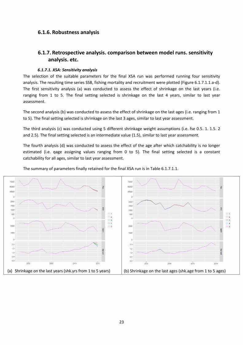
6.1.7.1. XSA: Sensitivity analysis

The selection of the suitable parameters for the final XSA run was performed running four sensitivity

analysis. The resulting time series SSB, fishing mortality and recruitment were plotted (Figure 6.1.7.1.1.a-d).

The first sensitivity analysis (a) was conducted to assess the effect of shrinkage on the last years (i.e.

ranging from 1 to 5. The final setting selected is shrinkage on the last 4 years, similar to last year

assessment.

The second analysis (b) was conducted to assess the effect of shrinkage on the last ages (i.e. ranging from 1

to 5). The final setting selected is shrinkage on the last 3 ages, similar to last year assessment.

The third analysis (c) was conducted using 5 different shrinkage weight assumptions (i.e. fse 0.5. 1. 1.5. 2

and 2.5). The final setting selected is an intermediate value (1.5), similar to last year assessment.

The fourth analysis (d) was conducted to assess the effect of the age after which catchability is no longer

estimated (i.e. qage assigning values ranging from 0 to 5). The final setting selected is a constant

catchability for all ages, similar to last year assessment.

The summary of parameters finally retained for the final XSA run is in Table 6.1.7.1.1.

(a) Shrinkage on the last years (shk.yrs from 1 to 5 years)

(b) Shrinkage on the last ages (shk.age from 1 to 5 ages)

24

(c) Shrinkage weight (fse. 0.5. 1. 1.5. 2 and 2.5)

(d) Catchability (qage values ranging from 0 to 5)

Figure 6.1.7.1.1. Hake in GSA 7. Sensitivity analysis on shrinkage on the last years (a), last ages (b), weight

of the shrinkage (c), catchability at age (d).

Table 6.1.7.1.1: Hake in GSA 7. XSA settings.

Fse shk.yrs shk.ages rage qage

1.5 4 3 -1 5

6.1.7.2. XSA: Retrospective analysis

A retrospective analysis was conducted on recruitment, mean F and SSB (Figure 6.1.7.2.1) to ensure the

robustness of the final estimates. The results considering SSB don’t show any particularity, but the

recruitment and the mean F seems to be underestimated.

Figure 6.1.7.2.1. Hake in GSA 7. Retrospective analysis performed with XSA (Recruitment. mean F and SSB).

25

6.1.8. Assessment quality

Stability of the assessment, evaluation of quality of the data and reliability of model assumptions

are described in the 6.1.5-7 section.

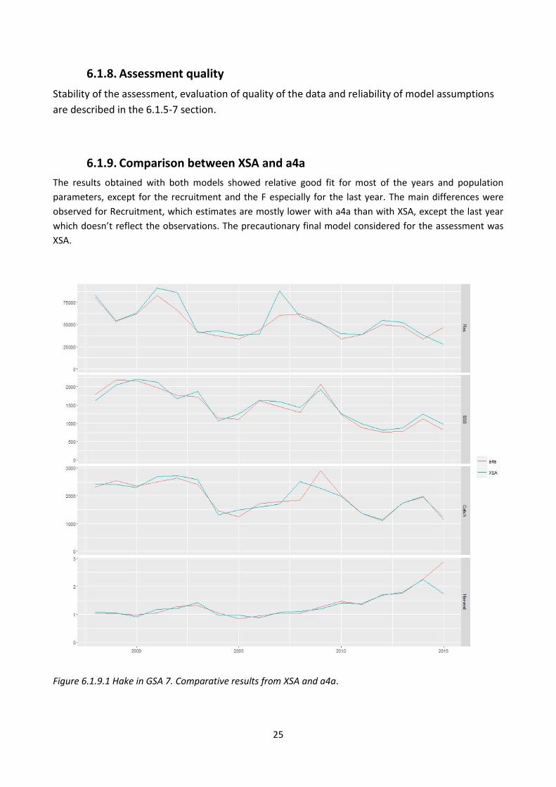
6.1.9. Comparison between XSA and a4a

The results obtained with both models showed relative good fit for most of the years and population

parameters, except for the recruitment and the F especially for the last year. The main differences were

observed for Recruitment, which estimates are mostly lower with a4a than with XSA, except the last year

which doesn’t reflect the observations. The precautionary final model considered for the assessment was

XSA.

Figure 6.1.9.1 Hake in GSA 7. Comparative results from XSA and a4a.

26

7. Stock predictions

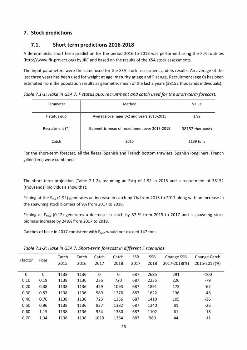
7.1. Short term predictions 2016-2018

A deterministic short term prediction for the period 2016 to 2018 was performed using the FLR routines

(http://www.flr-project.org) by JRC and based on the results of the XSA stock assessments.

The input parameters were the same used for the XSA stock assessment and its results. An average of the

last three years has been used for weight at age, maturity at age and F at age, Recruitment (age 0) has been

estimated from the population results as geometric mean of the last 3 years (38152 thousands individuals).

Table 7.1-1: Hake in GSA 7. F status quo. recruitment and catch used for the short-term forecast.

Parameter Method Value

F status quo Average over ages 0-2 and years 2013-2015 1.92

Recruitment (*) Geometric mean of recruitment over 2013-2015 38152 thousands

Catch 2015 1139 tons

For the short-term forecast, all the fleets (Spanish and French bottom trawlers, Spanish longliners, French

gillnetters) were combined.

The short term projection (Table 7.1-2), assuming an Fstq of 1.92 in 2015 and a recruitment of 38152

(thousands) individuals show that:

Fishing at the Fstq (1.92) generates an increase in catch by 7% from 2015 to 2017 along with an increase in

the spawning stock biomass of 9% from 2017 to 2018.

Fishing at FMSY (0.12) generates a decrease in catch by 87 % from 2015 to 2017 and a spawning stock

biomass increase by 249% from 2017 to 2018.

Catches of hake in 2017 consistent with FMSY would not exceed 147 tons.

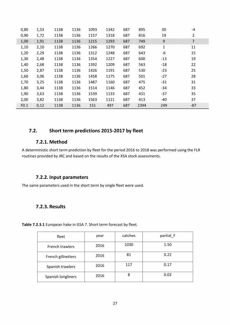
Table 7.1-2: Hake in GSA 7. Short-term forecast in different F scenarios.

Ffactor Fbar Catch

2015

Catch

2016

Catch

2017

Catch

2018

SSB

2017

SSB

2018

Change SSB

2017-2018(%)

Change Catch

2015-2017(%)

0 0 1138 1136 0 0 687 2685 291 -100

0,10 0,19 1138 1136 236 720 687 2235 226 -79

0,20 0,38 1138 1136 429 1093 687 1891 175 -62

0,30 0,57 1138 1136 589 1276 687 1622 136 -48

0,40 0,76 1138 1136 723 1356 687 1410 105 -36

0,50 0,96 1138 1136 837 1382 687 1240 81 -26

0,60 1,15 1138 1136 934 1380 687 1102 61 -18

0,70 1,34 1138 1136 1019 1364 687 989 44 -11

27

0,80 1,53 1138 1136 1093 1342 687 895 30 -4

0,90 1,72 1138 1136 1157 1318 687 816 19 2

1,00 1,91 1138 1136 1215 1293 687 749 9 7

1,10 2,10 1138 1136 1266 1270 687 692 1 11

1,20 2,29 1138 1136 1312 1248 687 643 -6 15

1,30 2,48 1138 1136 1354 1227 687 600 -13 19

1,40 2,68 1138 1136 1392 1209 687 563 -18 22

1,50 2,87 1138 1136 1426 1191 687 530 -23 25

1,60 3,06 1138 1136 1458 1175 687 501 -27 28

1,70 3,25 1138 1136 1487 1160 687 475 -31 31

1,80 3,44 1138 1136 1514 1146 687 452 -34 33

1,90 3,63 1138 1136 1539 1133 687 431 -37 35

2,00 3,82 1138 1136 1563 1121 687 413 -40 37

F0.1 0,12 1138 1136 151 497 687 2394 249 -87

7.2. Short term predictions 2015-2017 by fleet

7.2.1. Method

A deterministic short term prediction by fleet for the period 2016 to 2018 was performed using the FLR

routines provided by JRC and based on the results of the XSA stock assessments.

7.2.2. Input parameters

The same parameters used in the short term by single fleet were used.

7.2.3. Results

Table 7.2.3.1 European hake in GSA 7. Short term forecast by fleet.

fleet year catches partial_F

French trawlers 2016 1030 1.50

French gillnetters 2016 81 0.22

Spanish trawlers 2016 117 0.17

Spanish longliners 2016 8 0.02

28

7.3. Medium term predictions

No medium term forecast has been performed. because of lacking of a reliable stock-recruitment relationship.

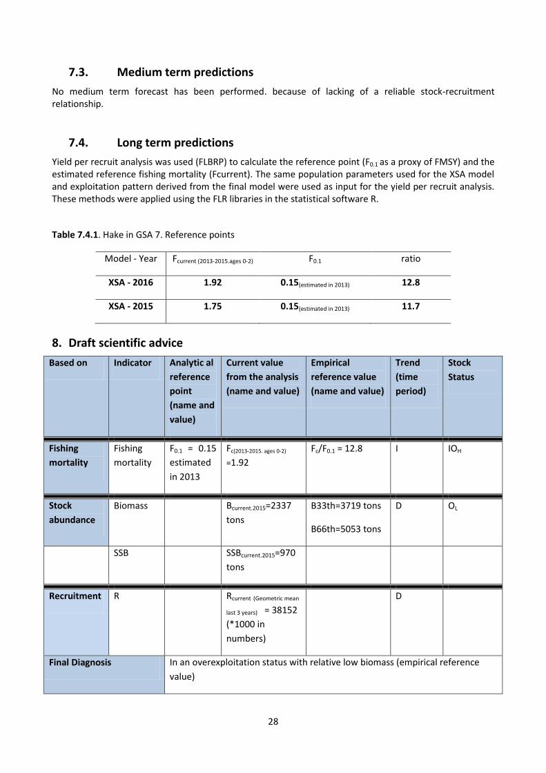
7.4. Long term predictions

Yield per recruit analysis was used (FLBRP) to calculate the reference point (F0.1 as a proxy of FMSY) and the estimated reference fishing mortality (Fcurrent). The same population parameters used for the XSA model and exploitation pattern derived from the final model were used as input for the yield per recruit analysis. These methods were applied using the FLR libraries in the statistical software R.

Table 7.4.1. Hake in GSA 7. Reference points

Model - Year Fcurrent (2013-2015.ages 0-2) F0.1 ratio

XSA - 2016 1.92 0.15(estimated in 2013) 12.8

XSA - 2015 1.75 0.15(estimated in 2013) 11.7

8. Draft scientific advice

Based on Indicator Analytic al

reference

point

(name and

value)

Current value

from the analysis

(name and value)

Empirical

reference value

(name and value)

Trend

(time

period)

Stock

Status

Fishing

mortality

Fishing

mortality

F0.1 = 0.15

estimated

in 2013

Fc(2013-2015. ages 0-2)

=1.92

Fc/F0.1 = 12.8 I IOH

Stock

abundance

Biomass Bcurrent.2015=2337

tons

B33th=3719 tons

B66th=5053 tons

D OL

SSB SSBcurrent.2015=970

tons

Recruitment R Rcurrent (Geometric mean

last 3 years) = 38152

(*1000 in

numbers)

D

Final Diagnosis In an overexploitation status with relative low biomass (empirical reference

value)

29

This stock is in an overexploitation status with a relative low biomass. Since 2010, the fishing

mortality has reached the highest levels of the time series. Moreover, spawning stock biomass and

recruitment are at the lowest levels of the series, without any sign of improvement. The current

exploitation level is well above the level estimated to be sustainable, despite the important

decrease in number of French trawlers since 2011, reducing the number of boats by almost 50%.

This stock is still in a high overexploitation status.

Management advice and recommendations: Reduce fishing mortality

-Respect the minimum legal landing size and legal mesh size

-Spatio-temporal closures for the protection of nurseries and spawning zones

-Reduce number of days at sea and/or numbers of boats

-Respect the freezing of the effort in the Fishery Restricted Area

30

9. Explanation of codes

Trend categories

1) N - No trend 2) I - Increasing 3) D – Decreasing 4) C - Cyclic

Stock Status

Based on Fishing mortality related indicators

1) N - Not known or uncertain – Not much information is available to make a judgment; 2) U - undeveloped or new fishery - Believed to have a significant potential for expansion in

total production; 3) S - Sustainable exploitation- fishing mortality or effort below an agreed fishing mortality or

effort based Reference Point; 4) IO –In Overfishing status– fishing mortality or effort above the value of the agreed fishing

mortality or effort based Reference Point. An agreed range of overfishing levels is provided;

Range of Overfishing levels based on fishery reference points

In order to assess the level of overfishing status when F0.1 from a Y/R model is used

as LRP. the following operational approach is proposed:

If Fc*/F0.1 is below or equal to 1.33 the stock is in (OL): Low overfishing

If the Fc/F0.1 is between 1.33 and 1.66 the stock is in (OI): Intermediate overfishing

If the Fc/F0.1 is equal or above to 1.66 the stock is in (OH): High overfishing

*Fc is current level of F

5) C- Collapsed- no or very few catches;

Based on Stock related indicators

1) N - Not known or uncertain: Not much information is available to make a judgment 2) S - Sustainably exploited: Standing stock above an agreed biomass based Reference Point; 3) O - Overexploited: Standing stock below the value of the agreed biomass based Reference

Point. An agreed range of overexploited status is provided;

Empirical Reference framework for the relative level of stock biomass index

Relative low biomass: Values lower than or equal to 33rd percentile of biomass index in the time series (OL)

Relative intermediate biomass: Values falling within this limit and 66th percentile (OI)

Relative high biomass: Values higher than the 66th percentile (OH)

31

4) D – Depleted: Standing stock is at lowest historical levels. irrespective of the amount of fishing effort exerted;

5) R –Recovering: Biomass are increasing after having been depleted from a previous period;

Agreed definitions as per SAC Glossary

Overfished (or overexploited) - A stock is considered to be overfished when its abundance is below

an agreed biomass based reference target point. like B0.1 or BMSY. To apply this denomination. it

should be assumed that the current state of the stock (in biomass) arises from the application of

excessive fishing pressure in previous years. This classification is independent of the current level of

fishing mortality.

Stock subjected to overfishing (or overexploitation) - A stock is subjected to overfishing if the

fishing mortality applied to it exceeds the one it can sustainably stand. for a longer period. In other

words. the current fishing mortality exceeds the fishing mortality that. if applied during a long

period. under stable conditions. would lead the stock abundance to the reference point of the

target abundance (either in terms of biomass or numbers)

Stock Assessment Form Demersal species - Archimer

Documents

Transcript of Stock Assessment Form Demersal species - Archimer