Determination of stress fields in the elastic lithosphere by methods based on stress orientations
23
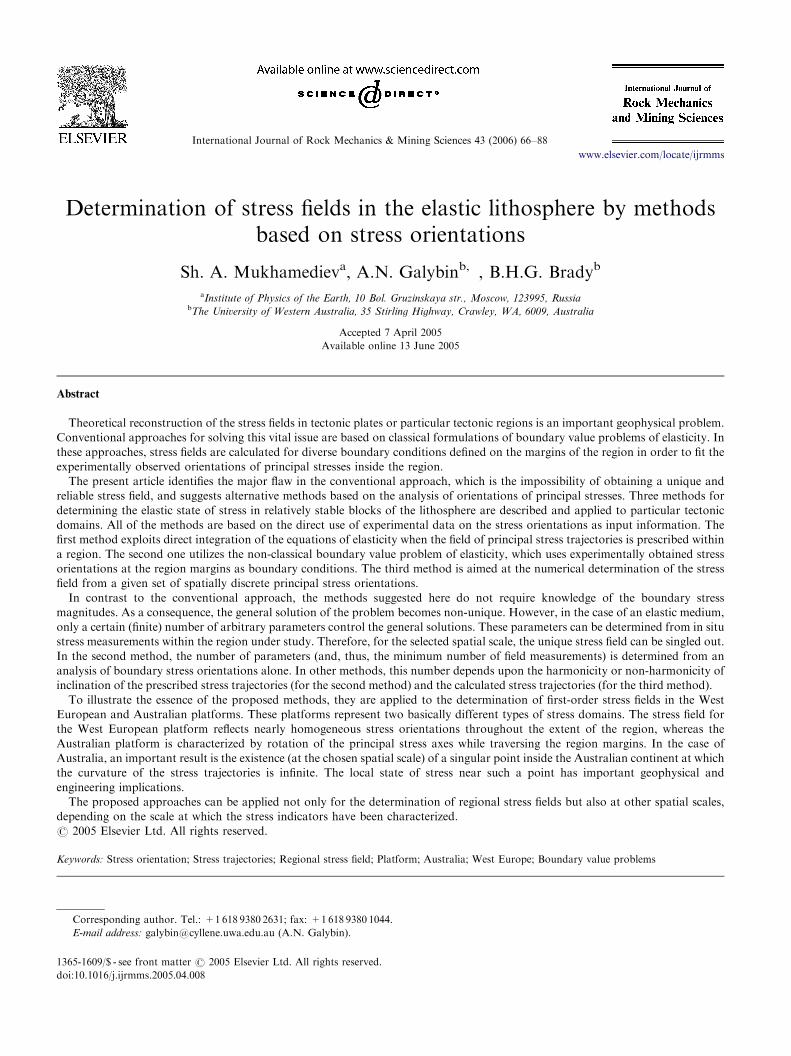
ARTICLE IN PRESS International Journal of Rock Mechanics & Mining Sciences 43 (2006) 66–88 Determination of stress fields in the elastic lithosphere by methods based on stress orientations Sh. A. Mukhamediev a , A.N. Galybin b, , B.H.G. Brady b a Institute of Physics of the Earth, 10 Bol. Gruzinskaya str., Moscow, 123995, Russia b The University of Western Australia, 35 Stirling Highway, Crawley, WA, 6009, Australia Accepted 7 April 2005 Available online 13 June 2005 Abstract Theoretical reconstruction of the stress fields in tectonic plates or particular tectonic regions is an important geophysical problem. Conventional approaches for solving this vital issue are based on classical formulations of boundary value problems of elasticity. In these approaches, stress fields are calculated for diverse boundary conditions defined on the margins of the region in order to fit the experimentally observed orientations of principal stresses inside the region. The present article identifies the major flaw in the conventional approach, which is the impossibility of obtaining a unique and reliable stress field, and suggests alternative methods based on the analysis of orientations of principal stresses. Three methods for determining the elastic state of stress in relatively stable blocks of the lithosphere are described and applied to particular tectonic domains. All of the methods are based on the direct use of experimental data on the stress orientations as input information. The first method exploits direct integration of the equations of elasticity when the field of principal stress trajectories is prescribed within a region. The second one utilizes the non-classical boundary value problem of elasticity, which uses experimentally obtained stress orientations at the region margins as boundary conditions. The third method is aimed at the numerical determination of the stress field from a given set of spatially discrete principal stress orientations. In contrast to the conventional approach, the methods suggested here do not require knowledge of the boundary stress magnitudes. As a consequence, the general solution of the problem becomes non-unique. However, in the case of an elastic medium, only a certain (finite) number of arbitrary parameters control the general solutions. These parameters can be determined from in situ stress measurements within the region under study. Therefore, for the selected spatial scale, the unique stress field can be singled out. In the second method, the number of parameters (and, thus, the minimum number of field measurements) is determined from an analysis of boundary stress orientations alone. In other methods, this number depends upon the harmonicity or non-harmonicity of inclination of the prescribed stress trajectories (for the second method) and the calculated stress trajectories (for the third method). To illustrate the essence of the proposed methods, they are applied to the determination of first-order stress fields in the West European and Australian platforms. These platforms represent two basically different types of stress domains. The stress field for the West European platform reflects nearly homogeneous stress orientations throughout the extent of the region, whereas the Australian platform is characterized by rotation of the principal stress axes while traversing the region margins. In the case of Australia, an important result is the existence (at the chosen spatial scale) of a singular point inside the Australian continent at which the curvature of the stress trajectories is infinite. The local state of stress near such a point has important geophysical and engineering implications. The proposed approaches can be applied not only for the determination of regional stress fields but also at other spatial scales, depending on the scale at which the stress indicators have been characterized. r 2005 Elsevier Ltd. All rights reserved. Keywords: Stress orientation; Stress trajectories; Regional stress field; Platform; Australia; West Europe; Boundary value problems www.elsevier.com/locate/ijrmms 1365-1609/$ - see front matter r 2005 Elsevier Ltd. All rights reserved. doi:10.1016/j.ijrmms.2005.04.008 Corresponding author. Tel.: +1 618 9380 2631; fax: +1 618 9380 1044. E-mail address: [email protected] (A.N. Galybin).
Transcript of Determination of stress fields in the elastic lithosphere by methods based on stress orientations
ARTICLE IN PRESS
1365-1609/$ - se
doi:10.1016/j.ijr
�CorrespondE-mail addr
International Journal of Rock Mechanics & Mining Sciences 43 (2006) 66–88
www.elsevier.com/locate/ijrmms
Determination of stress fields in the elastic lithosphere by methodsbased on stress orientations
Sh. A. Mukhamedieva, A.N. Galybinb,�, B.H.G. Bradyb
aInstitute of Physics of the Earth, 10 Bol. Gruzinskaya str., Moscow, 123995, RussiabThe University of Western Australia, 35 Stirling Highway, Crawley, WA, 6009, Australia
Accepted 7 April 2005
Available online 13 June 2005
Abstract
Theoretical reconstruction of the stress fields in tectonic plates or particular tectonic regions is an important geophysical problem.
Conventional approaches for solving this vital issue are based on classical formulations of boundary value problems of elasticity. In
these approaches, stress fields are calculated for diverse boundary conditions defined on the margins of the region in order to fit the
experimentally observed orientations of principal stresses inside the region.
The present article identifies the major flaw in the conventional approach, which is the impossibility of obtaining a unique and
reliable stress field, and suggests alternative methods based on the analysis of orientations of principal stresses. Three methods for
determining the elastic state of stress in relatively stable blocks of the lithosphere are described and applied to particular tectonic
domains. All of the methods are based on the direct use of experimental data on the stress orientations as input information. The
first method exploits direct integration of the equations of elasticity when the field of principal stress trajectories is prescribed within
a region. The second one utilizes the non-classical boundary value problem of elasticity, which uses experimentally obtained stress
orientations at the region margins as boundary conditions. The third method is aimed at the numerical determination of the stress
field from a given set of spatially discrete principal stress orientations.
In contrast to the conventional approach, the methods suggested here do not require knowledge of the boundary stress
magnitudes. As a consequence, the general solution of the problem becomes non-unique. However, in the case of an elastic medium,
only a certain (finite) number of arbitrary parameters control the general solutions. These parameters can be determined from in situ
stress measurements within the region under study. Therefore, for the selected spatial scale, the unique stress field can be singled out.
In the second method, the number of parameters (and, thus, the minimum number of field measurements) is determined from an
analysis of boundary stress orientations alone. In other methods, this number depends upon the harmonicity or non-harmonicity of
inclination of the prescribed stress trajectories (for the second method) and the calculated stress trajectories (for the third method).
To illustrate the essence of the proposed methods, they are applied to the determination of first-order stress fields in the West
European and Australian platforms. These platforms represent two basically different types of stress domains. The stress field for
the West European platform reflects nearly homogeneous stress orientations throughout the extent of the region, whereas the
Australian platform is characterized by rotation of the principal stress axes while traversing the region margins. In the case of
Australia, an important result is the existence (at the chosen spatial scale) of a singular point inside the Australian continent at which
the curvature of the stress trajectories is infinite. The local state of stress near such a point has important geophysical and
engineering implications.
The proposed approaches can be applied not only for the determination of regional stress fields but also at other spatial scales,
depending on the scale at which the stress indicators have been characterized.
r 2005 Elsevier Ltd. All rights reserved.
Keywords: Stress orientation; Stress trajectories; Regional stress field; Platform; Australia; West Europe; Boundary value problems
e front matter r 2005 Elsevier Ltd. All rights reserved.
mms.2005.04.008
ing author. Tel.: +1618 9380 2631; fax: +1618 9380 1044.
ess: [email protected] (A.N. Galybin).
ARTICLE IN PRESSS.A. Mukhamediev et al. / International Journal of Rock Mechanics & Mining Sciences 43 (2006) 66–88 67
1. Introduction
The determination of in situ stresses in the Earth’scrust is based upon the inversion of data on varioustypes of natural stress indicators such as earth-quake focal mechanisms, alignments of geologicalstructures, stress induced borehole ‘‘breakouts’’, etc.[1]. This information is mostly used to provide theorientation of the principal stresses and sometimes thetype of stress regime, which can be extensional (normalfaulting), strike-slip or compressive (thrust faulting).The observations of stress orientations have beenanalysed and summarized in the World Stress Map(WSM) database [2–4] for a large number of locationsover the globe. In rock mechanics and rock engineering,the importance of knowledge of the state of stress inrock and methods for its estimation have been reviewedin the Special Issue of the IJRMMS (2003, Vol. 40,Issues 7–8): Rock Stress Estimation, ISRM SuggestedMethods and Associated Supporting Papers ([5–7] andthe others).Despite its importance, the stress state of the Earth’s
crust is still far from being fully characterized, becausethe stress magnitudes remain unknown in most cases.Therefore, considerable effort has recently beenapplied to determine regional stress fields by mathema-tical modelling. Among others, the West Europeanplatform and the Indo-Australian plate (IAP) havebeen the focus of numerous studies devoted toreconstruction of the regional stress state (e.g., [8–14]).In these studies, the stress fields are calculated by solvinga number of boundary value problems of elasticityusually posed in terms of stresses. This presumes thatthe boundary stresses are chosen either hypothetically orfrom model considerations such that the calculatedorientations of the principal stresses fit the observedstress orientations. However, diverse boundaryconditions may produce the same stress orientations(e.g., [11]), which manifests the non-uniqueness of theresults obtained by this approach. Considering theresults of stress field modelling in the IAP, Coblentz etal. [11] pessimistically conclude that ‘‘this non-unique-ness continues to make modelling the IAP stress fieldproblematic’’ and that ‘‘a more complete understanding(of the intraplate stress field) awaits a better under-standing of the relative magnitudes of the boundaryforces’’.The present paper suggests an alternative appro-
ach for the determination of the regional stressfields in the elastic lithosphere. In contrast to theconventional method considered briefly above, theapproach discussed below employs the experi-mental data on stress orientations as input informa-tion rather than as constraints on the solutionswhich are sought. It can be considered as a directformulation of the solution for the stress field. Three
separate methods are considered within the frameworkof this approach:
1.
the direct integration of the equilibrium equations,given the stress trajectory field;2.
solution of a non-classical boundary value problemwhich uses the stress orientations as the boundaryconditions;3.
determination of the stress field by proper interpola-tion of the spatially discrete stress orientations.For purposes of illustrating the solution procedure,in-plane stresses within the West European and Aus-tralian platforms are analysed here. In the study, wemainly concentrate on a novel methodology for thedetermination of the stress fields for stable regions of thelithosphere, so that only first-order simple analyticalsolutions describing these stress fields are derived byusing the first two methods listed above. However, thesolutions presented might be considered as plausiblealternatives to the results of previous studies and caneasily be revised to take into account second-orderfeatures of the stress orientation pattern.
2. Methods for the determination of stress fields
2.1. Theoretical background for the 2-D stress state
determination
Many stress measurements indicate that two of threeprincipal stress in the Earth’s upper crust are sub-horizontal (e.g., [1,2]). Thus, 2-D stress fields are usuallyconsidered in modelling the regional stress state. In thiscase, the in-plane symmetric stress tensor T given by itscomponents T11, T12, T22 in a Cartesian coordinatesystem Ox1x2 can be described by means of thefollowing stress functions [15]
P ¼1
2ðT11 þ T22Þ; D ¼
1
2ðT22 � T11Þ þ iT12. (1)
Here the functions P and D represent the spherical anddeviatoric parts of the stress tensor respectively. Thestress function P is real-valued while the function D is acomplex-valued function of the independent variablesz ¼ x1 þ ix2; z ¼ x1 � ix2. (See Appendix A for defini-tion of notation and manipulations with functionsdepending on z and z.) The functions P and D satisfytwo equilibrium equations which can be expressed in thefollowing complex form
qP
qz¼
qD
qz. (2)
In this formulation, in-plane body forces are neglected.The functions P and D can also be expressed through
the maximum compressive in-plane stress, SH;max, and

ARTICLE IN PRESSS.A. Mukhamediev et al. / International Journal of Rock Mechanics & Mining Sciences 43 (2006) 66–8868
minimum compressive in-plane stress, SH;min, as follows:
P ¼ �1
2ðSH;max þ SH;minÞ; D ¼ tmaxeia,
tmax ¼1
2ðSH;max � SH;minÞ, ð3Þ
where the modulus tmax ¼ jDj represents the in-planemaximum shear stress and a ¼ argðDÞ is the argument ofthe function D. It can be expressed by the angle j of theinclination of SH;max to the x1-axis as
a ¼ �2j. (4)
The angle j is measured anti-clockwise from thepositive direction of the x1-axis.Any 2-D stress field (also called the T -field) can be
fully characterized by three scalar fields. These can bethe three scalar fields Pðz; zÞ, tmaxðz; zÞ, and aðz; zÞ oralternatively SH;maxðz; zÞ, SH;minðz; zÞ, and jðz; zÞ. Thelatter determines the field of the trajectories of principalstress (the j-field).1 The principal stress trajectoriesform the curvilinear orthogonal net inside the region,which consists of two families: the family of SH;maxtrajectories and the family of SH;min trajectories.Given the j-field, the T-field can be obtained,
regardless of the constitutive equations of the medium,by integrating the equilibrium equations (2). Thesebecome a closed system of partial differential equationsfor the determination of the real-valued functions P andtmax [17,18]. When considering a statically determinedgeomaterial, an extra relationship is imposed onfunctions P, tmax , and a in addition to equilibriumequations (2).For the special case of an homogeneous isotropic
elastic medium, besides the equilibrium conditions (2)one has the following supplementary equation imposedon the mean stress P:
DP ¼ 0, (5)
where D is the Laplace operator defined by formula(A.3). The stress functions P and D according to theKolosov-Muskhelishvili formulae [15] have the form
Pðz; zÞ ¼ FðzÞ þ FðzÞ; Dðz; zÞ ¼ zF0ðzÞ þCðzÞ (6)
where the complex potentials FðzÞ, CðzÞ are holo-morphic functions whereas D is a bi- holomorphicfunction.2 Eqs. (6) represent the general solution of aplane elastic problem for a homogeneous isotropic bodysubject to small deformations and negligible bodyforces.Further, it will be demonstrated how the stresses
inside the elastic region can be determined in different
1Curves which are tangential at each point to the principal axes of
stress are known as trajectories of the principal stress [16].2The definition of holomorphic and bi-holomorphic functions and
some of their properties are discussed in Appendix A.
ways without appealing to boundary stress magnitudes:
1.
If the j-field is given, the equations of equilibrium areintegrated by the technique proposed by Mukhame-diev and Galybin [19] (see also Appendix B).2.
Given the SH;max orientations and the curvatures ofthe SH;max trajectory along the margin of the region,the boundary value problem of elasticity consideredby Galybin and Mukhamediev [20] is solved (see alsoAppendix C ).3.
If principal stress orientations are known at spatiallydiscrete points (which is the usual practice ingeophysics), then the T-field is calculated numericallyby means of an algorithm proposed by Galybin andMukhamediev [21,22].Other constitutive models can also be examined in theframework of the proposed approach. Examples arefound in various models of plasticity. The condition ofideal plasticity tmax ¼ const, which seems to be suitablefor modelling large scale stress state in seismically activeregions, leads to the following equation Im ðq2eia=qz2Þ ¼
0 [18] which is of hyperbolic type and imposed on the j-field alone. Another example is the relationship tmax ¼Cð�ð2=3ÞP þ ð1=3ÞSv � Pf Þ where Sv is the verticalprincipal stress corresponding to the load of the over-burden, Pf is the hydrostatic pore pressure, and para-meter C depends on frictional coefficient. Townend andZoback [23] proposed this relationship to describe thestate of failure equilibrium of intraplate continental crust.This is in agreement with the well-known Mises-Schleicher plasticity criterion (e.g., [24]), although cor-rected to take water content into account. For laterallyhomogeneous Sv and Pf it results in a system of two realequations imposed on two stress functions, which can berepresented in either the following complex form:
qP
qz¼ �
2
3CqPeia
qzor
qtmaxqz
¼ �2
3Cqtmaxeia
qz.
However the approach remains the same: to make thefull use of the experimental data on stress orientations.The problems 2 and 3 listed above for elasticity can beposed for other statically determined bodies in a similarway, except that in the case of hyperbolic governingequations, the boundary conditions on SH;max orienta-tions and curvatures of SH;max trajectory are prescribedon a part of the boundary rather than on the entiremargin of the region.When considering stress fields in stable blocks of the
lithosphere, we focus on the elastic model for tworeasons:
(i)
in this methodological paper we intend to comparethe results with those obtained by conventionalmathematical modelling which in most cases uses themodel of the elastic lithosphere;
ARTICLE IN PRESSS.A. Mukhamediev et al. / International Journal of Rock Mechanics & Mining Sciences 43 (2006) 66–88 69
(ii)
often the experimental data on stress orientationshave been obtained with the use (explicit or implicit)of elasticity (e.g., survey [5]).It should be noted that the data on stress orientationsare available through the World Stress Map database(www.world-stress-map.org). The official 2003 release ofthe database [4] has been used in this study. It contained13600 points around the globe, which are of differentquality ranked according to a quality ranking schemedeveloped in [2,3]. The best quality A (about 5% of alldata) records data with the accuracy of 710�151; dataof B-(14%, 715�201) and C-(59%, 7251) quality arealso recommended for including into stress maps. In allexamples considered in this study, we use data of A–Cquality, which means that the data are quite scattered.This fact justifies the model of planar plates applied forstudying stress fields in Western Europe and Australia.It is believed that the account for sphericity of theearth’s crust will be within the errors due to datascattering.Disregard of possible lateral body forces caused by
lateral variations of density and width of the litho-sphere deserves discussion as follows. Firstly, we notethat the possible influence of lateral inhomogeneities isalready reflected in real stress orientations, which areused as input. However, this circumstance alonedoes not justify the neglecting horizontal body force.One has to prove that application of this force doesnot affect the calculated fields tmaxðz; zÞ and aðz; zÞ.Fortunately, in 2D elasticity it is valid for a wideclass of horizontal body forces, namely for theforces which possess harmonic potential. Let the vectorof lateral body force, bðz; zÞ ¼ b1 þ ib2 , be expressed asb ¼ qP=qz where Pðz; zÞ is the potential of lateral bodyforce. Then all the equations of elasticity remainvalid in the form presented in (2), (5) if P is understoodas P þP and Pðz; zÞ is a harmonic function, DP ¼ 0.Thus, the introduction of the vector b disturbsneither principal stress orientations nor maximum shearstresses. It only influences the magnitudes of SH;maxðz; zÞand SH;min z; zð Þ by adding to them the sameamount which can be different from point to point. Asfar as the stress deviator D is concerned, it can becalculated without account for b provided that themethod does not require to calculate (or prescribe)stress magnitudes separately as in the proposedapproach. Conventional methods, however, requireseparate consideration of the stress magnitudes, forinstance, when posing boundary conditions. It alsoshould be noted that the real inhomogeneitiesproducing horizontal body forces can be approximatedby introducing a harmonic potential P. Therefore we donot explicitly introduce horizontal body forces informulation of the considered boundary valueproblems. Moreover, an example for the Australian
stress field presented in Section 3.2 demonstrates that incontrast to conventional methods we do not need tointroduce lateral body forces in order to explain somefeatures of the examined stress field. There exist howeversome inelastic regions (as the Alps in Western Europe)in which horizontal body forces can affect stressorientations.
2.2. Determination of the stress field from given stress
trajectories in the lithosphere of arbitrary rheology
Suppose stress orientations are known at manylocations within the region, allowing compilation ofthe trajectories of principal stress (e.g., based on themethod proposed by Hansen and Mount [25] ). Then thej-field is known and the two unknowns SH;max andSH;min can be found by solving the set of twoequations of equilibrium. This set is a system ofpartial differential equations of hyperbolic type withcharacteristics that coincide with the trajectories ofprincipal stresses [17]. In order to obtain the T -field, thefollowing types of boundary value problems can beconsidered: the Cauchy (initial value) problem,the Goursat (characteristic) problem, and the mixedproblem.It is important that the magnitudes of SH;max and
SH;min have to be specified on a part of the boundary toobtain the complete solution within a certain part of theregion. Thus, the self-equilibrated T -field determined byits j-field contains two arbitrary functions, each of thembeing dependent on a single real variable. For thesimplest case when body forces are absent and theSH;max trajectories are inclined at a constant angle j0 ¼�a0=2 to the x1-axis, the following expressions [17]define the SH;max and SH;min fields:
SH;maxðz; zÞ ¼ F ðs1Þ; SH;minðz; zÞ ¼ Gðs2Þ, (7)
where
s1 ¼1
2ðizeij0 � ize�ij0 Þ; s2 ¼
1
2ðzeij0 þ ze�ij0Þ (8)
The arbitrary functions F and G are to be defined fromthe boundary conditions.It should be emphasized that in the case considered,
there is no need to assume any constitutive model for theregion under study. However, a particular constitutivemodel would have been used for the determination ofthe local SH;max orientations. For instance, the modelcould be described by the constitutive equations ofplasticity if the stress orientations were reconstructedfrom data on irreversible fault slips (earthquake focalmechanisms, striations, etc., details of which areprovided in [26]).
ARTICLE IN PRESSS.A. Mukhamediev et al. / International Journal of Rock Mechanics & Mining Sciences 43 (2006) 66–8870
2.3. Determination of the elastic stress field by stress
trajectories given inside a region
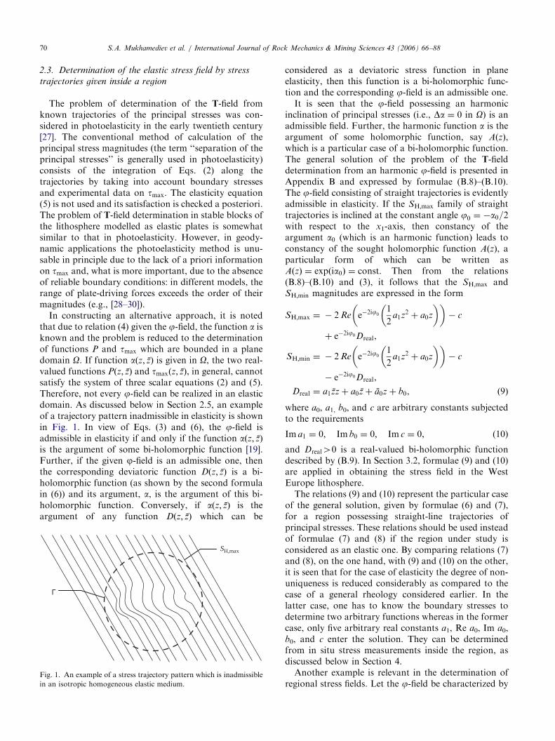
The problem of determination of the T-field fromknown trajectories of the principal stresses was con-sidered in photoelasticity in the early twentieth century[27]. The conventional method of calculation of theprincipal stress magnitudes (the term ‘‘separation of theprincipal stresses’’ is generally used in photoelasticity)consists of the integration of Eqs. (2) along thetrajectories by taking into account boundary stressesand experimental data on tmax. The elasticity equation(5) is not used and its satisfaction is checked a posteriori.The problem of T-field determination in stable blocks ofthe lithosphere modelled as elastic plates is somewhatsimilar to that in photoelasticity. However, in geody-namic applications the photoelasticity method is unu-sable in principle due to the lack of a priori informationon tmax and, what is more important, due to the absenceof reliable boundary conditions: in different models, therange of plate-driving forces exceeds the order of theirmagnitudes (e.g., [28–30]).In constructing an alternative approach, it is noted
that due to relation (4) given the j-field, the function a isknown and the problem is reduced to the determinationof functions P and tmax which are bounded in a planedomain O. If function aðz; zÞ is given in O, the two real-valued functions Pðz; zÞ and tmaxðz; zÞ, in general, cannotsatisfy the system of three scalar equations (2) and (5).Therefore, not every j-field can be realized in an elasticdomain. As discussed below in Section 2.5, an exampleof a trajectory pattern inadmissible in elasticity is shownin Fig. 1. In view of Eqs. (3) and (6), the j-field isadmissible in elasticity if and only if the function aðz; zÞis the argument of some bi-holomorphic function [19].Further, if the given j-field is an admissible one, thenthe corresponding deviatoric function Dðz; zÞ is a bi-holomorphic function (as shown by the second formulain (6)) and its argument, a, is the argument of this bi-holomorphic function. Conversely, if aðz; zÞ is theargument of any function Dðz; zÞ which can be
Γ
SH,max
Fig. 1. An example of a stress trajectory pattern which is inadmissible
in an isotropic homogeneous elastic medium.
considered as a deviatoric stress function in planeelasticity, then this function is a bi-holomorphic func-tion and the corresponding j-field is an admissible one.It is seen that the j-field possessing an harmonic
inclination of principal stresses (i.e., Da ¼ 0 in O) is anadmissible field. Further, the harmonic function a is theargument of some holomorphic function, say AðzÞ,which is a particular case of a bi-holomorphic function.The general solution of the problem of the T-fielddetermination from an harmonic j-field is presented inAppendix B and expressed by formulae (B.8)–(B.10).The j-field consisting of straight trajectories is evidentlyadmissible in elasticity. If the SH;max family of straighttrajectories is inclined at the constant angle j0 ¼ �a0=2with respect to the x1-axis, then constancy of theargument a0 (which is an harmonic function) leads toconstancy of the sought holomorphic function AðzÞ, aparticular form of which can be written asAðzÞ ¼ expðia0Þ ¼ const. Then from the relations(B.8)–(B.10) and (3), it follows that the SH;max andSH;min magnitudes are expressed in the form
SH;max ¼ � 2Re e�2ij01
2a1z
2 þ a0z
� �� �� c
þ e�2ij0Dreal,
SH;min ¼ � 2Re e�2ij01
2a1z
2 þ a0z
� �� �� c
� e�2ij0Dreal,
Dreal ¼ a1zz þ a0z þ a0z þ b0, ð9Þ
where a0, a1, b0, and c are arbitrary constants subjectedto the requirements
Im a1 ¼ 0; Im b0 ¼ 0; Im c ¼ 0, (10)
and Dreal40 is a real-valued bi-holomorphic functiondescribed by (B.9). In Section 3.2, formulae (9) and (10)are applied in obtaining the stress field in the WestEurope lithosphere.The relations (9) and (10) represent the particular case
of the general solution, given by formulae (6) and (7),for a region possessing straight-line trajectories ofprincipal stresses. These relations should be used insteadof formulae (7) and (8) if the region under study isconsidered as an elastic one. By comparing relations (7)and (8), on the one hand, with (9) and (10) on the other,it is seen that for the case of elasticity the degree of non-uniqueness is reduced considerably as compared to thecase of a general rheology considered earlier. In thelatter case, one has to know the boundary stresses todetermine two arbitrary functions whereas in the formercase, only five arbitrary real constants a1, Re a0, Im a0,b0, and c enter the solution. They can be determinedfrom in situ stress measurements inside the region, asdiscussed below in Section 4.Another example is relevant in the determination of
regional stress fields. Let the j-field be characterized by
ARTICLE IN PRESS
0 1
0
1
x1
0
A
B
-1
-1
Fig. 2. The pattern of SH;max orientations in the vicinity of a singular
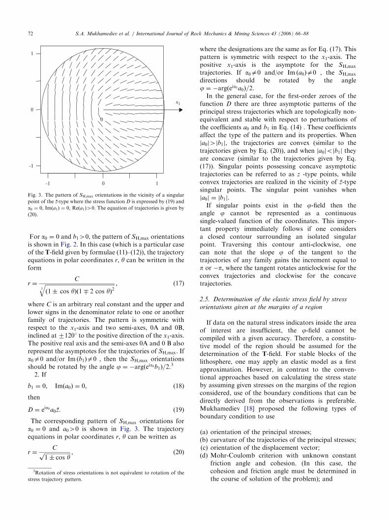
point of the z-type where the stress function D is expressed by (16) and
a0 ¼ 0, Imðb1Þ ¼ 0, Reðb1Þ40. The equation of the trajectories is givenby (17).
S.A. Mukhamediev et al. / International Journal of Rock Mechanics & Mining Sciences 43 (2006) 66–88 71
a trajectory inclination j ¼ j02y=2, where y is thepolar angle. Then from Eq. (4), expðiaÞ ¼expð�2ij0Þ expðiyÞ and the function AðzÞ can be takenin the form AðzÞ ¼ expðia0Þz, where a0 ¼ �2j0. From(B.8)–(B.10), the general solution for the T-field in termsof the functions D and P can be written as follows:
Dðz; zÞ ¼ eia0zDrealðz; zÞ,
Drealðz; zÞ ¼ a2zz þ a1z þ a1z þ b1,
Pðz; zÞ ¼ 2Re eia01
3a2z
3 þ1
2a1z
2
� �� �þ c, ð11Þ
where
Im a2 ¼ 0; Im b1 ¼ 0; Im c ¼ 0. (12)
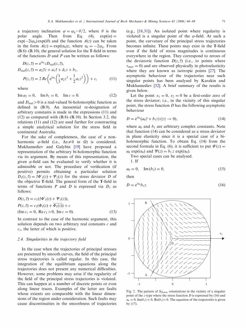
and Dreal40 is a real-valued bi-holomorphic function asdefined in (B.9). An inessential re-designation ofarbitrary constants is made in the expressions (11) and(12) as compared with (B.8)–(B.10). In Section 3.2, therelations (11) and (12) are used further for constructinga simple analytical solution for the stress field incontinental Australia.For the sake of completeness, the case of a non-
harmonic j-field (i.e., Daa0 in O) is considered.Mukhamediev and Galybin [19] have proposed arepresentation of the arbitrary bi-holomorphic functionvia its argument. By means of this representation, thegiven j-field can be evaluated to verify whether it isadmissible or not. The procedure of verification (ifpositive) permits obtaining a particular solutionD1ðz; zÞ ¼ zF0
1ðzÞ þC1ðzÞ for the stress deviator D ofthe objective T-field. The general form of the T-field interms of functions P and D is expressed via D1 asfollows:
Dðz; zÞ ¼ c1ðzF01ðzÞ þC1ðzÞÞ,
Pðz; zÞ ¼ c1ðF1ðzÞ þ F1ðzÞÞ þ c
ðIm c1 ¼ 0; Re c140; Im c ¼ 0Þ. ð13Þ
In contrast to the case of the harmonic argument, thissolution depends on two arbitrary real constants c andc1, the latter of which is positive.
2.4. Singularities in the trajectory field
In the case when the trajectories of principal stressesare presented by smooth curves, the field of the principalstress trajectories is called regular. In this case, theintegration of the equilibrium equations along thetrajectories does not present any numerical difficulties.However, some problems may arise if the regularity ofthe field of the principal stress trajectories is violated.This can happen at a number of discrete points or evenalong linear traces. Examples of the latter are faultswhose extents are comparable with the linear dimen-sions of the region under consideration. Such faults maycause discontinuities in the smoothness of trajectories
(e.g., [18,31]). An isolated point where regularity isviolated is a singular point of the j-field. At such apoint, the curvature of the principal stress trajectoriesbecomes infinite. These points may exist in the T-fieldeven if the field of stress magnitudes is continuouseverywhere in the region. They correspond to zeroes ofthe deviatoric function Dðz; zÞ (i.e., to points wheretmax ¼ 0) and are observed physically in photoelasticitywhere they are known as isotropic points [27]. Theasymptotic behaviour of the trajectories near suchsingular points has been analysed by Karakin andMukhamediev [32]. A brief summary of the results isgiven below.Let the point x1 ¼ 0, x2 ¼ 0 be a first-order zero of
the stress deviator; i.e., in the vicinity of this singularpoint, the stress function D has the following asymptoticbehaviour
D ¼ eia0 ða0z þ b1zÞ ðjzj ! 0Þ, (14)
where a0 and b1 are arbitrary complex constants. Notethat function (14) can be considered as a stress deviatorin plane elasticity since it is a special case of a bi-holomorphic function. To obtain Eq. (14) from thesecond formula in Eq. (6), it is sufficient to put F0ðzÞ ¼
a0 expðia0Þ and CðzÞ ¼ b1 z expðia0Þ.Two special cases can be analysed.1. If
a0 ¼ 0; Im ðb1Þ ¼ 0, (15)
then
D ¼ eia0b1z. (16)
ARTICLE IN PRESS
-1 0 1
-1
0
1
x1
0
Fig. 3. The pattern of SH;max orientations in the vicinity of a singular
point of the z-type where the stress function D is expressed by (19) and
a0 ¼ 0, Imða1Þ ¼ 0, Reða1Þ40. The equation of trajectories is given by(20).
S.A. Mukhamediev et al. / International Journal of Rock Mechanics & Mining Sciences 43 (2006) 66–8872
For a0 ¼ 0 and b140, the pattern of SH;max orientationsis shown in Fig. 2. In this case (which is a particular caseof the T-field given by formulae (11)–(12)), the trajectoryequations in polar coordinates r, y can be written in theform
r ¼Cffiffiffiffiffiffiffiffiffiffiffiffiffiffiffiffiffiffiffiffiffiffiffiffiffiffiffiffiffiffiffiffiffiffiffiffiffiffiffiffiffiffiffiffiffiffiffiffiffiffiffi
ð1 cos yÞð1 2 cos yÞ23
q , (17)
where C is an arbitrary real constant and the upper andlower signs in the denominator relate to one or anotherfamily of trajectories. The pattern is symmetric withrespect to the x1-axis and two semi-axes, 0A and 0B,inclined at71201 to the positive direction of the x1-axis.The positive real axis and the semi-axes 0A and 0 B alsorepresent the asymptotes for the trajectories of SH;max. Ifa0a0 and/or Im ðb1Þa0 , then the SH;max orientationsshould be rotated by the angle j ¼ �argðeia0b1Þ=2.
3
2. If
b1 ¼ 0; Imða0Þ ¼ 0, (18)
then
D ¼ eia0a0z. (19)
The corresponding pattern of SH;max orientations fora0 ¼ 0 and a040 is shown in Fig. 3. The trajectoryequations in polar coordinates r, y can be written as
r ¼Cffiffiffiffiffiffiffiffiffiffiffiffiffiffiffiffiffiffiffi
1 cos yp , (20)
3Rotation of stress orientations is not equivalent to rotation of the
stress trajectory pattern.
where the designations are the same as for Eq. (17). Thispattern is symmetric with respect to the x1-axis. Thepositive x1-axis is the asymptote for the SH;maxtrajectories. If a0a0 and/or Im ða0Þa0 , the SH;maxdirections should be rotated by the anglej ¼ �argðeia0a0Þ=2.In the general case, for the first-order zeroes of the
function D there are three asymptotic patterns of theprincipal stress trajectories which are topologically non-equivalent and stable with respect to perturbations ofthe coefficients a0 and b1 in Eq. (14) . These coefficientsaffect the type of the pattern and its properties. Whenja0j4jb1j, the trajectories are convex (similar to thetrajectories given by Eq. (20)), and when ja0jojb1j theyare concave (similar to the trajectories given by Eq.(17)). Singular points possessing concave asymptotictrajectories can be referred to as z -type points, whileconvex trajectories are realized in the vicinity of z-typesingular points. The singular point vanishes whenja0j ¼ jb1j.If singular points exist in the j-field then the
angle j cannot be represented as a continuoussingle-valued function of the coordinates. This impor-tant property immediately follows if one considersa closed contour surrounding an isolated singularpoint. Traversing this contour anti-clockwise, onecan note that the slope j of the tangent to thetrajectories of any family gains the increment equal top or �p, where the tangent rotates anticlockwise for theconvex trajectories and clockwise for the concavetrajectories.
2.5. Determination of the elastic stress field by stress
orientations given at the margins of a region
If data on the natural stress indicators inside the areaof interest are insufficient, the j-field cannot becompiled with a given accuracy. Therefore, a constitu-tive model of the region should be assumed for thedetermination of the T-field. For stable blocks of thelithosphere, one may apply an elastic model as a firstapproximation. However, in contrast to the conven-tional approaches based on calculating the stress stateby assuming given stresses on the margins of the regionconsidered, use of the boundary conditions that can bedirectly derived from the observations is preferable.Mukhamediev [18] proposed the following types ofboundary condition to use
(a)
orientation of the principal stresses; (b) curvature of the trajectories of the principal stresses; (c) orientation of the displacement vector; (d) Mohr-Coulomb criterion with unknown constantfriction angle and cohesion. (In this case, thecohesion and friction angle must be determined inthe course of solution of the problem); and
ARTICLE IN PRESSS.A. Mukhamediev et al. / International Journal of Rock Mechanics & Mining Sciences 43 (2006) 66–88 73
(e)
surface force orientation (as proposed by Galybin[33]).4The proposed definition (22) agrees with the definition of the index
for holomorphic functions (e.g., [34]). In the latter case 2K (if positive)
is equal to the number of zeroes of the holomorphic function inside the
domain bounded by G provided that zeroes of n-order are counted n
times. This theorem is no longer valid for bi-holomorphic functions
due to the presence of zeroes of various types (i.e., the z � type singular
points can appear in addition to the z-type points which only are
inherent in the class of holomorphic functions).
The use of these boundary conditions does notrequire any additional hypotheses regarding the dis-tribution of stress, displacement and/or force magni-tudes over the entire boundary of the region. Theconditions (a) and (b) can be derived, for instance, fromthe stress indicators distributed in a relatively broadzone along the margins of the platform regions; theorientation of the displacement and force vectors in (c)and (e) can be determined on divergent and convergentlithospheric plate boundaries; the condition (d) issuitable for the part of the boundary coinciding with adeep fault.In the case of plane elasticity, two scalar-type
boundary conditions must be imposed on the wholeboundary of the region. These may consist of variouspairs of the above-mentioned boundary conditionsimposed on particular parts of the boundary. Thedifferent combinations of these conditions form the suiteof possible boundary value problems.The case when conditions (a) and (b) are given on the
entire boundary G of an elastic domain O has beeninvestigated in detail by Galybin and Mukhamediev[20]. It is shown that these conditions can equi-valently be replaced by the following conditions on thecontour G:
G : a ¼ aGðsÞ;qaqn
¼ a0nðsÞ. (21)
Here q=qn represents the derivative in the direction ofthe outward unit normal n to the contour G, and aGðsÞand a0nðsÞ are given functions of the arc length s alongthe contour.The solution of the elastic boundary value problem
defined by Eqs. (3) and (6) and boundary conditions (21)is not unique. To illustrate this, suppose a solution (i.e.,the functions Pðz; zÞ and Dðz; zÞ satisfying conditions(21)) be found. Then multiplication of P and D by anypositive real constant does not violate either theequilibrium or the boundary conditions. Similarly, ifthe function P is changed by adding an arbitrary realconstant, this would also be a valid solution. Such lineartransformations of the T-field do not disturb theprincipal stress orientations at any point inside theregion. Hence, the solution obtained is non-unique andshould be considered as one of many possible solutionsof the problem.These simplest transformations of the T-field do
not exhaust the variety of all possible solutions ofthe problem defined by Eqs. (3), (6), (21). As hasbeen shown by Galybin and Mukhamediev [20], thenumber of linearly independent solutions depends upon
the index 2K of the stress function D over G, determinedas follows.4
2K¼ IndGD ¼1
2p
ZGda ¼ �
1
p
ZGdj. (22)
Here relation (4) has been taken into account. It can beseen that the absolute value of the index is equal to thedoubled number of rotations of the principal stress axis(for instance, the SH;max-axis) after the complete circuitaround the contour. One can note that the number K ofrotations may be a half-integer quantity because theprincipal stress axis is not a vector and no direction isprescribed on it. The sign of the index is determined bythe sign of the difference between the number ofclockwise and anticlockwise rotations of the axis. Forinstance, the index would be negative if the axis has onlyrotated anticlockwise.For 2KX0, the problem (3), (6), (21) is always
solvable and its solution depends on a certain numberof arbitrary constants. For an arbitrary simply con-nected domain bounded by a smooth closed contourand for any non-negative index, 2K, the solutioncontains 8K+5 arbitrary real constants. For anynegative index 2Ko� 1 no bounded solutions exist.However it can be shown that unbounded solutions existif the functions F0ðzÞ and CðzÞ are allowed to have poles.Mechanically, this type of solution could be interpretedby the presence of concentrated forces and moments,dislocations, etc, inside the region.To illustrate the role of the index, 2K, Galybin and
Mukhamediev [20] considered a unit circle with thefollowing boundary conditions:
G : aG ¼ a0 þ 2Ky a0n ¼ 0; 2K ¼ 0;1;2 . . . (23)
where a0 ¼ const and y is the polar angle. Theseboundary conditions and corresponding solutions areillustrated in Fig. 4 for different indexes. Completeresults are presented in Appendix C. For 2K ¼ 22, nobounded solution exists (Fig. 4a). For 2K ¼ 21, thesolution for the stress function D depends only on asingle real constant a0, defined in formula (19) (Fig. 4b),for which the trajectories are described by formula (20).For 2K ¼ 0, the T-field, which depends on five realconstants, is expressed by formulae (9) and (10) andpossesses the uniform j-field depicted for a0 ¼ 0 in Fig.4c. It should be noted that in the cases 2K¼21 and2K ¼ 0, the T-field represents the unique field oftrajectories of the principal stresses in spite of possible
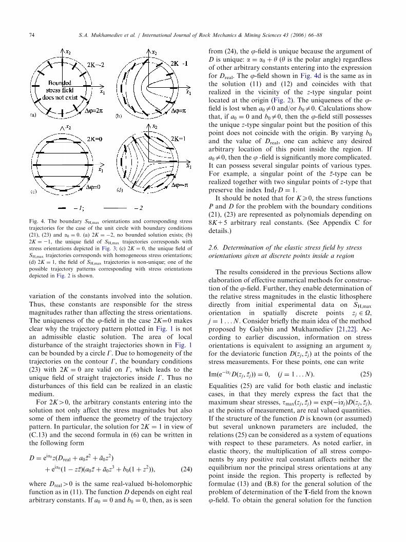
ARTICLE IN PRESS
Fig. 4. The boundary SH;max orientations and corresponding stress
trajectories for the case of the unit circle with boundary conditions
(21), (23) and a0 ¼ 0. (a) 2K ¼ �2, no bounded solution exists; (b)
2K ¼ 21, the unique field of SH;max trajectories corresponds with
stress orientations depicted in Fig. 3; (c) 2K ¼ 0, the unique field of
SH;max trajectories corresponds with homogeneous stress orientations;
(d) 2K ¼ 1, the field of SH;max trajectories is non-unique; one of the
possible trajectory patterns corresponding with stress orientations
depicted in Fig. 2 is shown.
S.A. Mukhamediev et al. / International Journal of Rock Mechanics & Mining Sciences 43 (2006) 66–8874
variation of the constants involved into the solution.Thus, these constants are responsible for the stressmagnitudes rather than affecting the stress orientations.The uniqueness of the j-field in the case 2K¼0 makesclear why the trajectory pattern plotted in Fig. 1 is notan admissible elastic solution. The area of localdisturbance of the straight trajectories shown in Fig. 1can be bounded by a circle G. Due to homogeneity of thetrajectories on the contour G, the boundary conditions(23) with 2K ¼ 0 are valid on G, which leads to theunique field of straight trajectories inside G. Thus nodisturbances of this field can be realized in an elasticmedium.For 2K40, the arbitrary constants entering into the
solution not only affect the stress magnitudes but alsosome of them influence the geometry of the trajectorypattern. In particular, the solution for 2K ¼ 1 in view of(C.13) and the second formula in (6) can be written inthe following form
D ¼ eia0zðDreal þ a0z2 þ a0z
2Þ
þ eia0ð1� zzÞða0z þ a0z3 þ b0ð1þ z2ÞÞ, ð24Þ
where Dreal40 is the same real-valued bi-holomorphicfunction as in (11). The function D depends on eight realarbitrary constants. If a0 ¼ 0 and b0 ¼ 0, then, as is seen
from (24), the j-field is unique because the argument ofD is unique: a ¼ a0 þ y (y is the polar angle) regardlessof other arbitrary constants entering into the expressionfor Dreal. The j-field shown in Fig. 4d is the same as inthe solution (11) and (12) and coincides with thatrealized in the vicinity of the z-type singular pointlocated at the origin (Fig. 2). The uniqueness of the j-field is lost when a0a0 and/or b0a0. Calculations showthat, if a0 ¼ 0 and b0a0, then the j-field still possessesthe unique z-type singular point but the position of thispoint does not coincide with the origin. By varying b0and the value of Dreal, one can achieve any desiredarbitrary location of this point inside the region. Ifa0a0, then the j -field is significantly more complicated.It can possess several singular points of various types.For example, a singular point of the z-type can berealized together with two singular points of z-type thatpreserve the index IndGD ¼ 1.It should be noted that for KX0, the stress functions
P and D for the problem with the boundary conditions(21), (23) are represented as polynomials depending on8K+5 arbitrary real constants. (See Appendix C fordetails.)
2.6. Determination of the elastic stress field by stress
orientations given at discrete points inside a region
The results considered in the previous Sections allowelaboration of effective numerical methods for construc-tion of the j-field. Further, they enable determination ofthe relative stress magnitudes in the elastic lithospheredirectly from initial experimental data on SH;maxorientation in spatially discrete points zj 2 O,j ¼ 1 . . .N. Consider briefly the main idea of the methodproposed by Galybin and Mukhamediev [21,22]. Ac-cording to earlier discussion, information on stressorientations is equivalent to assigning an argument aj
for the deviatoric function Dðzj ; zjÞ at the points of thestress measurements. For these points, one can write
Imðe�iaj Dðzj ; zjÞÞ ¼ 0; ðj ¼ 1 . . .NÞ. (25)
Equalities (25) are valid for both elastic and inelasticcases, in that they merely express the fact that themaximum shear stresses, tmaxðzj ; zjÞ ¼ expð�iajÞDðzj ; zjÞ,at the points of measurement, are real valued quantities.If the structure of the function D is known (or assumed)but several unknown parameters are included, therelations (25) can be considered as a system of equationswith respect to these parameters. As noted earlier, inelastic theory, the multiplication of all stress compo-nents by any positive real constant affects neither theequilibrium nor the principal stress orientations at anypoint inside the region. This property is reflected byformulae (13) and (B.8) for the general solution of theproblem of determination of the T-field from the knownj-field. To obtain the general solution for the function
ARTICLE IN PRESSS.A. Mukhamediev et al. / International Journal of Rock Mechanics & Mining Sciences 43 (2006) 66–88 75
D, any particular solution D1 is multiplied by anarbitrary positive constant or even by positive function.To avoid this ambiguity (at least for a non-harmonicargument), the tmax-field should be normalized by a realconstant. A possible way to do this is to postulate thatthe average modulus of D over the domain is unity, i.e.,
XN
j¼1
e�iaj Dðzj ; zjÞ ¼ N. (26)
In addition, the condition (26) helps to avoid the trivialsolution D 0.For the elastic lithosphere, the potentials F0 and C
entering the general solution (6) are presented in theform
CðzÞ ¼Xn
k¼0
ckRkðzÞ; F0ðzÞ ¼Xn�1k¼0
ckþnþ1RkðzÞ
ðNX4n þ 2Þ, ð27Þ
where RkðzÞ are given linearly independent holomorphicfunctions, and ck are complex constants sought in thesolution. By expressing Dðzj ; zjÞ in (25), (26) throughF0ðzjÞ, CðzjÞ via (27), using the second formula in (6) andintroducing the array X consisting of 4n+2 real valuedunknowns Xk defined by the relation ck ¼ Xk+iX2n+k+1,one can reduce the starting system (25), (26) to theredundant system of linear algebraic equations
AX ¼ B. (28)
In this expression, A is the (N+1)� (4n+2)-matrix ofthe system with real-valued components which areexpressed through the values of known functions atthe points zj, and B ¼ f0; . . . 0;NgT is the (N+1)-vectorin which all but one component is zero. The single non-zero component, N, is due to the condition of normal-ization expressed in Eq. (27). It is noted that the righthand side of the system (28) is known exactly, while thecomponents of the matrix A depend on data quality.This situation is different from what usually appears infitting problems, which are often ill-posed.The system (28) can be solved by the least squares
method provided that NX4n þ 2. The solution proce-dure becomes complicated when the matrix A is ill-conditioned, i.e. its rank is less then 4n+2. The mainsource that can cause the matrix A to be ill-conditionedis the harmonicity of argument a of the recovereddeviatoric function D. According to the results pre-sented in Section 2.3 and Appendix B, in this case fourarbitrary real valued constants entering the generalsolution for D do not influence the stress orientationand, therefore, cannot be determined from theseorientations. The condition (26) diminishes the numberof undeterminable constants to three, which ultimatelyleads to decrease of the rank of matrix A by three units.The matrix A can also be ill-conditioned due toexperimental errors in the stress orientation measure-
ments which, in principle, can introduce error inan initially well-posed problem. For example, theinitially non-harmonic j-field can tend to an harmonicone.To overcome the difficulties concerned with a poorly
posed problem, it is proposed to control the conditionnumber of matrix A during solving the system, whichgives an indication of whether the matrix is ill-conditioned or not. If the condition number is greaterthan a specified critical value, then the matrix A in (28) isreplaced by a close matrix A0 whose rank is less thanrank(A). The matrix A0 is close to A in the sense thattheir first singular values coincide. This idea is widelyused in image processing in order to reduce the amountof data stored or transmitted (e.g., [35,36]).
3. Solutions for particular tectonic regions
To illustrate the application of the proposed methodsof analysis and stress field reconstruction, the solutionsfor the elastic stress fields of the West European andAustralian platforms are presented in this Section.Simple analytical solutions for the first-order stressfields are obtained by means of the first and secondmethods discussed in Section 2.1. The West Europeanstress field, which possesses nearly straight trajectories,is determined by direct integration of the elasticityequations (the first method) while the Australian stressfield, exhibiting spatial variability of the SH;max orienta-tions, is obtained by solving the boundary valueproblem constructed on stress orientations (the secondmethod). Further, the stress fields for West Europe andAustralia are numerically investigated by the thirdmethod. Figs. 5 and 6 illustrate these solutions. Theexperimentally obtained orientations of SH;max are takenfrom [4], where they are quality ranked from A to E (Abeing the best quality) according to Zoback’s scheme [3].The number N of experimental points in Figs. 5 and 6varies according to the range of data quality that ischosen.
3.1. The West European stress field
A large amount of experimental data on in situstresses has been gathered over nearly a half-century ofstudying the stress state of the lithosphere of WesternEurope, from both instrumental measurements and theanalysis of natural stress indicators. Even the earlymeasurements made in the 1960s and early 1970s (e.g.,[37]) revealed a uniform NW orientation of the SH;maxaxis. They provided some constraints on the interpreta-tion of the tectonics and seismicity of large geologicalstructures such as the Rhine system of grabens [37,38].Later, new constraints on stresses were determined andthe existing data were generalized as a result of
ARTICLE IN PRESS
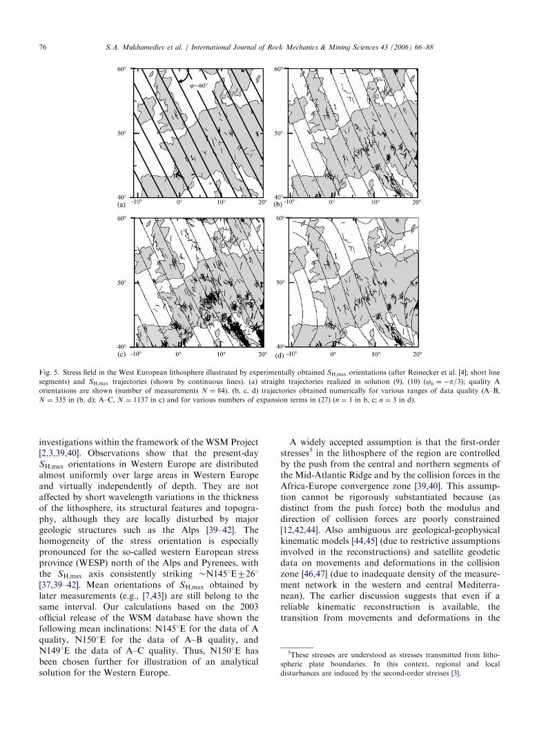
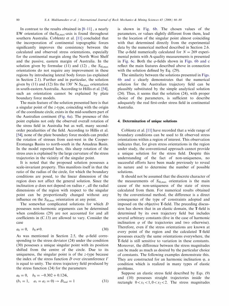
Fig. 5. Stress field in the West European lithosphere illustrated by experimentally obtained SH;max orientations (after Reinecker et al. [4]; short line
segments) and SH;max trajectories (shown by continuous lines). (a) straight trajectories realized in solution (9), (10) ðj0 ¼ �p=3Þ; quality Aorientations are shown (number of measurements N ¼ 84). (b, c, d) trajectories obtained numerically for various ranges of data quality (A–B,
N ¼ 335 in (b, d); A–C, N ¼ 1137 in c) and for various numbers of expansion terms in (27) (n ¼ 1 in b, c; n ¼ 3 in d).
5These stresses are understood as stresses transmitted from litho-
spheric plate boundaries. In this context, regional and local
disturbances are induced by the second-order stresses [3].
S.A. Mukhamediev et al. / International Journal of Rock Mechanics & Mining Sciences 43 (2006) 66–8876
investigations within the framework of the WSM Project[2,3,39,40]. Observations show that the present-daySH;max orientations in Western Europe are distributedalmost uniformly over large areas in Western Europeand virtually independently of depth. They are notaffected by short wavelength variations in the thicknessof the lithosphere, its structural features and topogra-phy, although they are locally disturbed by majorgeologic structures such as the Alps [39–42]. Thehomogeneity of the stress orientation is especiallypronounced for the so-called western European stressprovince (WESP) north of the Alps and Pyrenees, withthe SH;max axis consistently striking �N1451E7261[37,39–42]. Mean orientations of SH;max obtained bylater measurements (e.g., [7,43]) are still belong to thesame interval. Our calculations based on the 2003official release of the WSM database have shown thefollowing mean inclinations: N1451E for the data of Aquality, N1501E for the data of A–B quality, andN1491E the data of A–C quality. Thus, N1501E hasbeen chosen further for illustration of an analyticalsolution for the Western Europe.
A widely accepted assumption is that the first-orderstresses5 in the lithosphere of the region are controlledby the push from the central and northern segments ofthe Mid-Atlantic Ridge and by the collision forces in theAfrica-Europe convergence zone [39,40]. This assump-tion cannot be rigorously substantiated because (asdistinct from the push force) both the modulus anddirection of collision forces are poorly constrained[12,42,44]. Also ambiguous are geological-geophysicalkinematic models [44,45] (due to restrictive assumptionsinvolved in the reconstructions) and satellite geodeticdata on movements and deformations in the collisionzone [46,47] (due to inadequate density of the measure-ment network in the western and central Mediterra-nean). The earlier discussion suggests that even if areliable kinematic reconstruction is available, thetransition from movements and deformations in the
ARTICLE IN PRESS
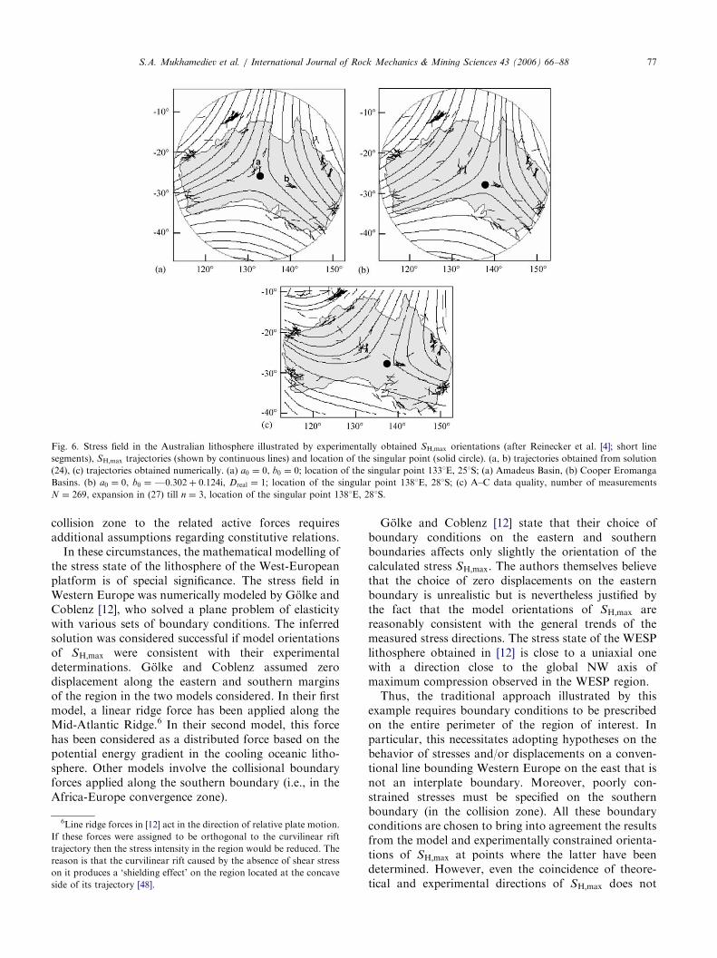
Fig. 6. Stress field in the Australian lithosphere illustrated by experimentally obtained SH;max orientations (after Reinecker et al. [4]; short line
segments), SH;max trajectories (shown by continuous lines) and location of the singular point (solid circle). (a, b) trajectories obtained from solution
(24), (c) trajectories obtained numerically. (a) a0 ¼ 0, b0 ¼ 0; location of the singular point 1331E, 251S; (a) Amadeus Basin, (b) Cooper Eromanga
Basins. (b) a0 ¼ 0, b0 ¼ F0:302þ 0:124i, Dreal ¼ 1; location of the singular point 1381E, 281S; (c) A–C data quality, number of measurements
N ¼ 269, expansion in (27) till n ¼ 3, location of the singular point 1381E, 281S.
S.A. Mukhamediev et al. / International Journal of Rock Mechanics & Mining Sciences 43 (2006) 66–88 77
collision zone to the related active forces requiresadditional assumptions regarding constitutive relations.In these circumstances, the mathematical modelling of
the stress state of the lithosphere of the West-Europeanplatform is of special significance. The stress field inWestern Europe was numerically modeled by Golke andCoblenz [12], who solved a plane problem of elasticitywith various sets of boundary conditions. The inferredsolution was considered successful if model orientationsof SH;max were consistent with their experimentaldeterminations. Golke and Coblenz assumed zerodisplacement along the eastern and southern marginsof the region in the two models considered. In their firstmodel, a linear ridge force has been applied along theMid-Atlantic Ridge.6 In their second model, this forcehas been considered as a distributed force based on thepotential energy gradient in the cooling oceanic litho-sphere. Other models involve the collisional boundaryforces applied along the southern boundary (i.e., in theAfrica-Europe convergence zone).
6Line ridge forces in [12] act in the direction of relative plate motion.
If these forces were assigned to be orthogonal to the curvilinear rift
trajectory then the stress intensity in the region would be reduced. The
reason is that the curvilinear rift caused by the absence of shear stress
on it produces a ‘shielding effect’ on the region located at the concave
side of its trajectory [48].
Golke and Coblenz [12] state that their choice ofboundary conditions on the eastern and southernboundaries affects only slightly the orientation of thecalculated stress SH;max. The authors themselves believethat the choice of zero displacements on the easternboundary is unrealistic but is nevertheless justified bythe fact that the model orientations of SH;max arereasonably consistent with the general trends of themeasured stress directions. The stress state of the WESPlithosphere obtained in [12] is close to a uniaxial onewith a direction close to the global NW axis ofmaximum compression observed in the WESP region.Thus, the traditional approach illustrated by this
example requires boundary conditions to be prescribedon the entire perimeter of the region of interest. Inparticular, this necessitates adopting hypotheses on thebehavior of stresses and/or displacements on a conven-tional line bounding Western Europe on the east that isnot an interplate boundary. Moreover, poorly con-strained stresses must be specified on the southernboundary (in the collision zone). All these boundaryconditions are chosen to bring into agreement the resultsfrom the model and experimentally constrained orienta-tions of SH;max at points where the latter have beendetermined. However, even the coincidence of theore-tical and experimental directions of SH;max does not
ARTICLE IN PRESSS.A. Mukhamediev et al. / International Journal of Rock Mechanics & Mining Sciences 43 (2006) 66–8878
guarantee the uniqueness and validity of the inferredstress field, because it is still fairly sensitive to the choiceof boundary stress magnitudes, as discussed in Section4.The application of the direct approach considered in
the present paper is free of the shortcomings ofconventional methods concerned with the necessity toimpose poorly constrained boundary conditions on thewhole perimeter of the region. Moreover, boundarystresses can be constrained from the solution itself. Themain idea is that, for the first-order stress field inWestern Europe, the trajectories can be approximatedby straight lines with the SH;max family inclined at anangle j0 ��601 (Fig. 5a) [49,50]. Then one can makeuse of the simple general solutions (7), (8) (if noassumptions on constitutive relations are made), and/or (9), (10) (for the elastic lithosphere), in which case j0should be taken as equal to �p=3.For the lithosphere of arbitrary rheology, the stress
field has been investigated by Mukhamediev [49]. Inorder to find the arbitrary functions F and G in (7), itwas assumed that the homogeneous trajectory patterncan be extended into the western and northwesternoceanic areas adjacent to continental West Europe. Thesolution was derived from two Cauchy problems, onewith boundary stresses prescribed along the segment ofthe Mid-Atlantic Ridge and the other with stresses givenon the southern boundary of the region (i.e., along theconvergence zone). In both cases, no stresses wereprescribed along the eastern boundary. The continuitycondition on the line separating the solution domains ofthe Cauchy problems imposes constraints on the vectortC of collision stresses. If its magnitude is known, thenits orientation is determined, and vice versa. The choiceof the actual direction of tC should be based on thecomparison between theoretically and experimentallydetermined stress regimes of the Western Europe litho-sphere, including instrumental measurements of stresses.Such a comparison showed that the vector tC is close (indirection) to the SH;max axis and experiences a counter-clockwise rotation on the southern boundary in theeastward direction. It is exactly the pattern of thecollision stresses that accounts for the presence of theobserved tensile stresses SH;min and strike-slip faultingregime in most of the WESP territory.If the lithosphere is assumed to be elastic, then the
necessity to impose boundary stresses is removed. Byapplying the method of direct integration of theelasticity equations (the first method) one has only tocompile a reliable pattern of trajectories of the principalstresses which are admissible for the elastic lithosphere.As a first approximation for the WESP domain, thestraight SH;max trajectories fitting the experimentallyobtained SH;max orientations immediately lead to thesolution given in (9) and (10). In Fig. 5a, theexperimental data of A-quality are shown for purposes
of judging how good the chosen approximation is. Theassumption about homogeneity of the stress trajectoriescan be verified through numerical solution of theproblem (i.e. the third method). Some results ofcalculation for various numbers of the SH;max orienta-tions taken into account and for various numbers ofterms in the expansion (27) are shown in Figs. 5b–d.It should be noted that with increasing n, the
calculations suggest some singular points appear nearthe boundaries of WESP (Fig. 5d). However, in contrastto the z-type singular point in continental Australia (asconsidered in Section 3.2), they are not stable. Thissuggests that they are probably artefacts caused byinconsistency of data and the degree of polynomials,rather than corresponding to real singularities. Thedomain located approximately within the range ofcoordinates 5–151E and 42–551N demonstrates a nearlyhomogeneous pattern of straight trajectories for n
varying up to 5. In the conceptual framework of ourapproach, this domain can be identified as WESP.
3.2. The Australian stress field
Experimentally determined elements of the state ofstress are known for various regions of Australia (e.g.,[51–54]). Although the number of reliable measurementsof stress orientations throughout continental Australiais much less than in Europe, it is believed that the first-order pattern of the field of stress orientations inAustralia (and even more broadly, within the IAP) isrelatively well established (e.g., [8–11]). In contrast toWestern Europe and eastern and central parts of NorthAmerica, where SH;max orientations are nearly uniform[2–4], the stress orientations in Australia show consider-able variation, as is evident in Fig. 6 . The main featuresof the stress pattern are the NE–SW orientation ofSH;max in the North West Shelf, the NNE–SSWorientation in central Australia (the Amadeus Basin)and roughly the E–W SH;max orientation throughout thesouthern part of the continent (more clearly defined insouth-western and south-eastern Australia). The sharprotation of the SH;max axis from E–W in the Cooper-Eromanga Basins to approximately N–S in the Ama-deus Basin should be noted especially (Fig. 6a).In a number of numerical studies, the observed
orientations have been used as constraints in numericalmodelling (e.g., [10]). In all these investigations, diversedistributions of forces acting on the boundary of theIAP have been assumed to model the regional stressstate in Australia. These assumptions have been justifiedby the hypothesis that the types of boundary forces areessentially different because the boundary includes anextensive mid-ocean ridge system to the south ofAustralia, and subduction zones and significant seg-ments of both continent-continent and continent-oceancollision to the north, north-west and east of Australia.
ARTICLE IN PRESSS.A. Mukhamediev et al. / International Journal of Rock Mechanics & Mining Sciences 43 (2006) 66–88 79
The ridge push force is usually assumed to be distributedover the area adjacent to the mid-ocean ridge. Thebuoyancy forces resulting from lithospheric densityvariation associated with continental margins andelevated continental crust can also be included (e.g.,[11]). As a rule, the drag at the base of the lithosphere isassumed to be constant over the area of the base of theplate and its magnitude is chosen to ensure mechanicalequilibrium, i.e. to provide zero resultant (net) torqueover the plate.Coblentz et al. [10] assumed that the torque associated
with the ridge push force is well constrained and theprincipal source of uncertainty can be ascribed to theboundary conditions used to represent the collisionalresistance and subduction zone forces acting along thenorthern boundary of the IAP. These poorly con-strained forces have been represented in their fourmodels in different ways. Based on their calculations,Coblentz et al. [10] have proposed that a number ofimportant features of the observed stress field within theAustralian continent can be explained in terms ofbalancing the ridge push torque with the resistancealong the Himalaya, Papua New Guinea, and NewZealand collisional boundary segments. They concludedthat many of the broad scale features of the observedstress orientations could be reproduced without appeal-ing either to the subduction or to the basal drag forces.Later Coblentz et al. [11] have extended the results to theIAP intraplate stress field.Cloetingh and Wortel [8,9] proposed that the rotation
of the stress orientations observed in the numericalstudies of the Australian continent is associated with itsgeographic location relatively close to the surroundingtrench segments (along the northern boundary of theIAP) and with the lateral variation of the pull forcesacting on the subsiding slabs.In these studies, if the main features of the boundary
forces have been accounted for, then the SH;maxorientation patterns obtained theoretically for theAustralian continent correspond roughly (at leastvisually) with the observed one. But for some over-simplified models [10,11], they are quite different. Thepredicted stress orientations along the Australianmargin do not exhibit rotation while traversing aroundthe contour. This important feature of the Australianstress field, that distinguishes it from other regions, istaken into account in the model proposed below.Regarding the stress magnitudes, one can note that inthe above-mentioned papers they are significantlydifferent from each other, even for visually closecorrespondence of model and field stress orientationpatterns. For example, the maximum magnitude of thecompressive stresses obtained by Coblentz et al. [10] isabout 25MPa, while the results of Cloetingh and Wortel[8,9] indicate that the level of the stress magnitudes forthe same region is around 100–200MPa.
From these results, it is concluded that the numericalmodelling of the stress field in the Australian continentis derived from a wide range of magnitudes ofpostulated plate-driving forces on the margins of theIAP. While the stress orientations may be modelledmore or less satisfactorily, the magnitudes of theseforces and the magnitudes of the calculated stressesinside the region remain highly controversial.The following unique characteristic of the Australian
stress field can be identified from analysis of naturalstress indicators (e.g., [2,3,55]) and from mathematicalmodelling (e.g., [8,9] ). This is the rotation of the SH;maxorientations. The observed discrete stress orientationsare consistent with the supposition that the SH;max-axisrotates clockwise at an angle of 1801 while going aroundthe continental margin anticlockwise. Thus the index 2Kin Eq. (22) is equal to unity. The simplest case ofrotation is considered further in the following analysis.For a polar coordinate system r, y , with origin locatedsomewhere within Australia, it is assumed that theinclination of the SH;max-axis changes proportionally tothe coordinate angle y. For the elastic model of thecontinental block, one can then reduce the problem ofthe regional stress determination to the problem (3), (6),(21), (23) with 2K ¼ 1. For simplicity, the functionsaGðyÞ and a0nðyÞ are assigned on a circle circumscribedaround Australia.The complex potentials F0ðzÞ, CðzÞ for this problem
are given by formulae (C.13) (see Appendix C) and thefunction D is presented by (24). A further simplificationcan be achieved if conditions
a0 ¼ 0; b0 ¼ 0, (29)
are imposed on the constants [50,56]. Then, aftersubstituting the potentials into formulae (6) andintegrating F0, one obtains expressions for the stressfunctions D and P given by Eqs. (11) and (12). It isevident that the argument of the function D is harmonic.The SH;max and SH;min magnitudes can be obtained fromEqs. (3), (11) and (12). The field of the SH;maxorientations corresponding to solution of Eqs. (11) and(12), for the case of Dreal40 and a0 ¼ 0, is presented inFig. 2.Because the stress orientations are non-sensitive to the
choice of a1, a2, and b1 in the solution given by (11) and(12), the argument a0 and the origin of the circle are theonly parameters to be varied in order to fit the observedpattern of the stress orientations. For Dreal40, the best(visual) congruence between the theoretical and fieldSH;max orientations is achieved if a0 � 2p=3 (x1-axes isassumed to be eastward-directed) and the origin of thecircle is located about 300 km to the SSE of theAmadeus Basin. Thus, the stress orientations depictedin Fig. 2 should be rotated clockwise by the anglej ¼ p=3. The result obtained for the stress trajectories isshown in Fig. 6a.
ARTICLE IN PRESSS.A. Mukhamediev et al. / International Journal of Rock Mechanics & Mining Sciences 43 (2006) 66–8880
In contrast to the results obtained in [8–11] , a nearlyEW orientation of theSH;max-axis is found throughoutsouthern Australia. Coblentz et al. [11] concluded thatthe incorporation of continental topographic forcessignificantly improves the consistency between thecalculated and observed stress orientations, especiallyfor the continental margin along the North West Shelfand the passive, eastern margin of Australia. In thesolution given by formulae (11) and (12) , the SH;maxorientations do not require any improvement in theseregions by introducing lateral body forces (as explainedin Section 2.1). Further and in particular, the solutiongiven by (11) and (12) fits the 1301 N SH;max orientationin south-eastern Australia. According to Hillis et al. [54],such an orientation cannot be explained by plateboundary force models.The main feature of the solution presented here is that
a singular point of the z-type, coinciding with the originof the coordinate circle, exists in the mid-southern part ofthe Australian continent (Fig. 6a). The presence of thispoint explains not only the observed overall rotation ofthe stress field in Australia but as well, many second-order peculiarities of the field. According to Hillis et al.[54], none of the plate boundary force models can predictthe rotation of stresses from east-west in the Cooper-Eromanga Basins to north-south in the Amadeus Basin.In the model reported here, this sharp rotation of thestress axes is explained by the large curvature of the stresstrajectories in the vicinity of the singular point.It is noted that the proposed solution possesses a
scale-invariant property. This manifests itself in that theratio of the radius of the circle, for which the boundaryconditions are posed, to the linear dimension of theregion does not affect the general solution. Since theinclination j does not depend on radius r , all the radialdimensions of the region with respect to the singularpoint can be proportionally changed without anyinfluence on the SH;max orientation at any point.The somewhat complicated solutions for which D
possesses non-harmonic arguments can be determinedwhen conditions (29) are not accounted for and allcoefficients in (C.13) are allowed to vary. Consider thecase
a0 ¼ 0; b0a0. (30)
As was mentioned in Section 2.5, the j-field corre-sponding to the stress deviator (24) under the condition(30) possesses a unique singular point with its positionshifted from the centre of the circle. Due to itsuniqueness, the singular point is of the z-type becausethe index of the stress function D over circumference Gis equal to unity. The stress trajectory field produced bythe stress function (24) for the parameters
a0 ¼ 0; b0 ¼ �0:302þ 0:124i,
ðb1 ¼ 1; a1 ¼ a2 ¼ 0Þ ! Dreal ¼ 1 ð31Þ
is shown in Fig. 6b. The chosen values of theparameters, or values slightly different from them, leadto the location of the singular point almost coincidingwith that determined directly from the experimentaldata by the numerical method described in Section 2.6.The j-field numerically calculated for N ¼ 269 experi-mental points with A-quality measurements is presentedin Fig. 6c. Both the j-fields shown in Figs. 6b and creflect the main features described above in connectionwith the solution defined by Eq. (29).The similarity between the solutions presented in Figs.
6b and c clearly demonstrates that the numericalsolution for the Australian trajectory field can beplausibly substituted by the simple analytical solution(24). Thus, it seems that the solution (24), with properchoice of the parameters, is sufficient to describeadequately the real first-order stress field in continentalAustralia.
4. Determination of unique solutions
Coblentz et al. [11] have recorded that a wide range ofboundary conditions can be used to fit observed stressorientations within a region of interest. This observationindicates that, for given stress orientations in the regionunder study, the conventional approach cannot providea unique solution for the stress field. Despite thisunderstanding of the fact of non-uniqueness, nosuccessful efforts have been made previously to revealits nature and to determine the number of possiblesolutions.It should not be assumed that the discrete character of
the measurements of SH;max orientation is the maincause of the non-uniqueness of the state of stresscalculated from them. For numerical results obtainedby the conventional method, the difference is a directconsequence of the type of‘ constraints adopted andimposed on the objective T-field. The preceding discus-sion has shown that in an elastic domain, the T-field isdetermined by its own trajectory field but includesseveral arbitrary constants (five in the case of harmonicinclination j of the trajectories and two otherwise).Therefore, even if the stress orientations are known atevery point of the region and the calculated T-fieldpossesses exactly the same orientations everywhere, theT-field is still sensitive to variation in these constants.Moreover, the difference between the stress magnitudescan be made as much as desired by the particular choiceof constants. The following examples demonstrate this.They are constructed for an harmonic inclination j, acondition which is realized in many types of elasticproblems.Suppose an elastic stress field described by Eqs. (9)
and (10) possesses straight trajectories inside therectangle 0ox1o1; 0ox2o2. The stress magnitudes
ARTICLE IN PRESS
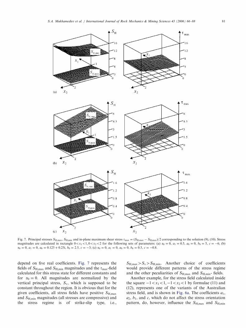
Fig. 7. Principal stresses SH;max, SH;min and in-plane maximum shear stress tmax ¼ ðSH;max � SH;maxÞ=2 corresponding to the solution (9), (10). Stressmagnitudes are calculated in rectangle 0ox1o1; 0ox2o2 for the following sets of parameters: (a) a0 ¼ 0, a1 ¼ 0:5, a0 ¼ 0, b0 ¼ 5, c ¼ �6; (b)
a0 ¼ 0, a1 ¼ 0, a0 ¼ 0:125þ 0:25i, b0 ¼ 2:5, c ¼ �3; (c) a0 ¼ 0, a1 ¼ 0, a0 ¼ 0, b0 ¼ 0:5, c ¼ �0:8.
S.A. Mukhamediev et al. / International Journal of Rock Mechanics & Mining Sciences 43 (2006) 66–88 81
depend on five real coefficients. Fig. 7 represents thefields of SH;max and SH;min magnitudes and the tmax-fieldcalculated for this stress state for different constants andfor a0 ¼ 0. All magnitudes are normalized by thevertical principal stress, Sv, which is supposed to beconstant throughout the region. It is obvious that for thegiven coefficients, all stress fields have positive SH;maxand SH;min magnitudes (all stresses are compressive) andthe stress regime is of strike-slip type, i.e.,
SH;max4Sv4SH;min. Another choice of coefficientswould provide different patterns of the stress regimeand the other peculiarities of SH;max and SH;min- fields.Another example, for the stress field calculated inside
the square �1ox1o1;�1ox2o1 by formulae (11) and(12), represents one of the variants of the Australianstress field, and is shown in Fig. 6a. The coefficients a1,a2, b1, and c, which do not affect the stress orientationpattern, do, however, influence the SH;max and SH;min
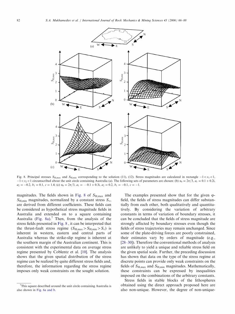
ARTICLE IN PRESS
W E S
N
S H,m
ax
4
3
2
1
0
S H,m
ax
4
3
2
1
0
S H,m
in
4
3
2
1
0
S H,m
in
4
3
2
1
0
WE S
NW
E S
NW
E S
NW
E S
(a)
(b)N
(c)
Fig. 8. Principal stresses SH;max and SH;min corresponding to the solution (11), (12). Stress magnitudes are calculated in rectangle �1ox1o1,�1ox2o1 circumscribed about the unit circle containing Australia (a). The following sets of parameters are chosen: (b) a0 ¼ 2p=3, a1 ¼ 0:1þ 0:2i,a2 ¼ �0:2, b1 ¼ 0:1, c ¼ 1:4; (c) a0 ¼ 2p=3, a1 ¼ F0:1þ 0:3i, a2 ¼ 0:2, b1 ¼ �0:1, c ¼ �1.
S.A. Mukhamediev et al. / International Journal of Rock Mechanics & Mining Sciences 43 (2006) 66–8882
magnitudes. The fields shown in Fig. 8 of SH;max andSH;min magnitudes, normalized by a constant stress Sv,are derived from different coefficients. These fields canbe considered as hypothetical stress magnitude fields inAustralia and extended on to a square containingAustralia (Fig. 8a).7 Then, from the analysis of thestress fields presented in Fig. 8 , it can be interpreted thatthe thrust-fault stress regime (SH;max4SH;min4Sv) isinherent in western, eastern and central parts ofAustralia whereas the strike-slip regime is inherent atthe southern margin of the Australian continent. This isconsistent with the experimental data on average stressregime presented by Coblentz et al. [10]. The analysisshows that the given spatial distribution of the stressregime can be realized by quite different stress fields and,therefore, the information regarding the stress regimeimposes only weak constraints on the sought solution.
7This square described around the unit circle containing Australia is
also shown in Fig. 6a and b.
The examples presented show that for the given j-field, the fields of stress magnitudes can differ substan-tially from each other, both qualitatively and quantita-tively. By considering the variation of arbitraryconstants in terms of variation of boundary stresses, itcan be concluded that the fields of stress magnitude arestrongly affected by boundary stresses even though thefields of stress trajectories may remain unchanged. Sincesome of the plate-driving forces are poorly constrained,their estimates vary by orders of magnitude (e.g.,[28–30]). Therefore the conventional methods of analysisare unlikely to yield a unique and reliable stress field onthe given spatial scale. Further, the preceding discussionhas shown that data on the type of the stress regime atdiscrete points can provide only weak constraints on thefields of SH;max and SH;min magnitudes. Mathematically,these constraints can be expressed by inequalitiesimposed on the combinations of the arbitrary constants.Stress fields in stable blocks of the lithospheres
obtained using the direct approach proposed here arealso non-unique. However, the degree of non-unique-
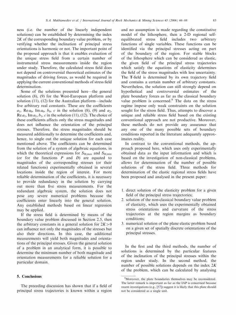
ARTICLE IN PRESSS.A. Mukhamediev et al. / International Journal of Rock Mechanics & Mining Sciences 43 (2006) 66–88 83
ness (i.e. the number of the linearly independentsolutions) can be established by determining the index2K of the corresponding boundary value problem, or byverifying whether the inclination of principal stressorientations is harmonic or not. The important point ofthe proposed approach is that it enables evaluation ofthe unique stress field from a certain number ofinstrumental stress measurements inside the regionunder study. Therefore, the calculated stress field doesnot depend on controversial theoretical estimates of themagnitudes of driving forces, as would be required inapplying the current conventional methods of stress fielddetermination.Some of the solutions presented here—the general
solution (8), (9) for the West-European platform andsolution (11), (12) for the Australian platform—includefive arbitrary real constants. These are the coefficientsa1, Re a0, Im a0, b0, c in the solution (8), (9) and a2,Re a1, Im a1, b1, c in the solution (11), (12). The choice ofthese coefficients affects only the stress magnitudes anddoes not influence the orientation of the principalstresses. Therefore, the stress magnitudes should bemeasured additionally to determine the coefficients and,hence, to single out the unique solution for each casementioned above. The coefficients can be determinedfrom the solution of a system of algebraic equations, inwhich the theoretical expressions for SH;max and SH;min(or for the functions P and D) are equated tomagnitudes of the corresponding stresses (or theirrelated functions) experimentally obtained in severallocations inside the region of interest. For morereliable determination of the coefficients, it is necessaryto provide redundancy in the solution by carryingout more than five stress measurements. For theredundant algebraic system, the solution does notpose any severe numerical problems because thecoefficients enter linearly into the general solution.Any established methods based on linear regressionmay be applied.If the stress field is determined by means of the
boundary value problem discussed in Section 2.5, thenthe arbitrary constants in a general solution for 2K40can influence not only the magnitudes of the stresses butalso their directions. In this case, the additionalmeasurements will yield both magnitudes and orienta-tions of the principal stresses. Given the general solutionof a problem in an analytical form, it is possible todetermine the minimum number of both magnitude andorientation measurements for a reliable solution for aparticular domain.
8Moreover, the plate boundaries themselves may be reconsidered.
The latter remark is important as far as the IAP is concerned because
recent investigations (e.g., [57]) suggest it is likely that this plate should
not be considered as a single unit.
5. Conclusions
The preceding discussion has shown that if a field ofprincipal stress trajectories is known within a region
and no assumption is made regarding the constitutivemodel of the lithosphere, then a 2-D regional self-equilibrated stress field includes two arbitraryfunctions of single variables. These functions can beidentified via the principal stresses acting on partof the boundary of the region. For stable blocksof the lithosphere which can be considered as elastic,the given field of the principal stress trajectorieswhich satisfy the equations of elasticity determinesthe field of the stress magnitudes with less uncertainty.The T-field is determined by its own trajectory fieldand contains a certain number of arbitrary constants.Nevertheless, the solution can still strongly depend onhypothetical and controversial estimates of theplate boundary forces as far as the classical boundaryvalue problem is concerned.8 The data on the stressregime impose only weak constraints on the solutionsought for the stress field. Thus, attempts to discover aunique and reliable stress field based on the existingconventional approach are not productive. Moreover,these methods do not provide any assurance thatany one of the many possible sets of boundaryconditions reported in the literature adequately approx-imates reality.In contrast to the conventional methods, the ap-
proach proposed here, which uses only experimentallyobtained data as the input information and which isbased on the investigation of non-classical problems,allows for determination of the number of possiblesolutions of the stress field. Three methods fordetermination of the elastic regional stress fields havebeen proposed and analysed in the present paper:
1.
direct solution of the elasticity problem for a givenfield of the principal stress trajectories;2.
solution of the non-classical boundary value problemof elasticity, which uses the experimentally obtainedstress orientations and curvature of the stresstrajectories at the region margins as boundaryconditions;3.
numerical solution of the plane elastic problem basedon a given set of spatially discrete orientations of theprincipal stresses.In the first and the third methods, the number ofsolutions is determined by the particular featuresof the inclination of the principal stresses within theregion under study. In the second method, thenumber of possible solutions depends on the index 2Kof the problem, which can be calculated by analysing
ARTICLE IN PRESSS.A. Mukhamediev et al. / International Journal of Rock Mechanics & Mining Sciences 43 (2006) 66–8884
the number of rotations of the principal stress axesmeasured while traversing the contour of theregion.The proposed methods have been applied to the
determination of two regional stress fields. For theessential part of the West European platform, whichexhibits an homogeneous field of nearly straighttrajectories, the analytical expression for the first-orderstress field depending on five arbitrary real constantswas obtained by means of the first method. The secondmethod was applied to the Australian platform, which ischaracterized by rotation of the principal stress axesalong the margin of the region. The third method wasused in both cases. By comparing analytical andnumerical results, it was concluded that the simpleanalytical expressions found for both regions arereasonable practical approximations for the real first-order stress fields.The arbitrary constants which are included in the
elastic solution for the principal stress magnitudes canbe found from the finite number of local in situstress measurements. This procedure enables singlingout the unique stress field. Moreover, if the directapproach is applied to the determination of the stressfield in a whole plate, then the plate-driving forces canbe obtained.For the boundary value problem posed for continen-
tal Australia, its solution index 2K is probably equal to1. One of the important results reported in the paper isthat this index suggests the existence of a singular pointinside the Australian continent. Singular points arecharacterized by equality of the principal stress magni-tudes (SH;max ¼ SH;min) and by locally infinite curvatureof the principal stress trajectories. The type and numberof singular points inside a domain determine both thelocal and block-scale characteristics of the geometry ofthe stress trajectory field. In particular, the existence ofthis point explains the sharp rotation of the SH;max axesin the central part of Australia. Such rotation cannot bepredicted by conventional models using plate boundaryforces. As for block-scale geometric characteristics ofthe stress field, singular points determine the number K
of full rotations of the SH;max axis in an anticlockwisetraverse of the contour of the region. Further, since thein-plane maximum shear stress tmax vanishes at thesingular point, in its vicinity there should be no seismicevents, or at least those exhibiting strike-slip faults. Theexistence of the singular point in Australia was firstreported by Mukhamediev et al. [56] in 1999 based onthe simplest solution (24), (29) for the continental stressfield. To the best of the authors’ knowledge, it is the firstsingular point detected in the lithosphere at the tectonicregional scale. The local state of stress associatedwith the existence of such a point has importantengineering implications for energy resource recoveryin the area.
Acknowledgments
The first author acknowledges the assistance providedby a Visiting Fellowship at The University of WesternAustralia supported by the ARC Large GrantsA89701652 (‘Induced seismicity and seismic sourcemechanisms in large-scale, deep level mining’) andA89600726 (‘Excavation and reinforcement design forunderground excavations subject to repeated dynamicloading). The last stage of the work was partlysupported by the Russian Foundation for BasicResearch and by the Section of the Earth’s Sciences ofRAS (fundamental program No. 5). Some helpfulcomments by Professor E T Brown on a draft of thepaper are recorded with gratitude.
Appendix A. Notation and definitions
This short appendix, which is similar to the Appendixin Galybin and Mukhamediev [20], introduces thenotation and derives necessary formulae used in themain text and Appendixes B and C.Any complex function f ðx1;x2Þ in a plane with
Cartesian coordinates x1,x2
f ¼ f 1ðx1; x2Þ þ if 2ðx1;x2Þ
ðf 1 ¼ Re f ; f 2 ¼ Im f Þ ðA:1Þ
can be considered as a function of conjugated complexvariables z ¼ x1 þ ix2, z ¼ x1 � ix2 and f ¼ f ðz; zÞ [58].The corresponding differential operators are
qqz
¼1
2
qqx1
� iqqx2
� �,
qqz
¼1
2
qqx1
þ iqqx2
� �. ðA:2Þ
The Laplace operator D is expressed in the form
D q2
qx2þ
q2
qy2¼ 4
q2
qzqz. (A.3)
The derivative of f in a direction determined by anyunit complex vector m ¼ m1 þ im2 ðjmj2 ¼ m21 þ m22 ¼
1Þ is defined as
qf
qm¼ m
qf
qzþ m
qf
qz. (A.4)
For real-valued function f (Im f ¼ 0) this derivative isalso real-valued.Let us consider a 2-D finite domain Xþ bounded by
the closed contour G (Fig. 9).
G : zðsÞ ¼ x1ðsÞ þ ix2ðsÞ, (A.5)
where z is a point on G, s is the arc length of G. Thepositive direction of traversing the contour G and thepositive directions of the unit tangent l ¼ l1 þ il2 andunit normal n ¼ n1 þ in2 vectors are shown in Fig. 9.
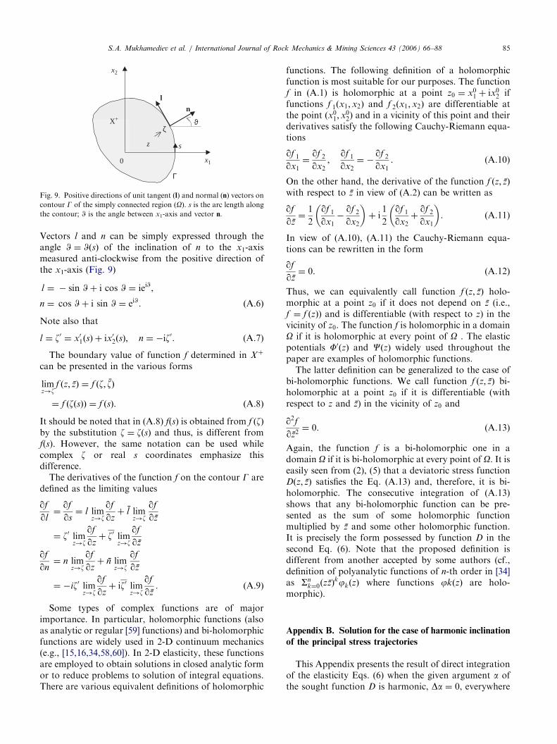
ARTICLE IN PRESS
x10
n
l
Γ
ζ
s
X+
z
x2
ϑ
Fig. 9. Positive directions of unit tangent (l) and normal (n) vectors on
contour G of the simply connected region (O). s is the arc length along
the contour; W is the angle between x1-axis and vector n.
S.A. Mukhamediev et al. / International Journal of Rock Mechanics & Mining Sciences 43 (2006) 66–88 85
Vectors l and n can be simply expressed through theangle W ¼ WðsÞ of the inclination of n to the x1-axismeasured anti-clockwise from the positive direction ofthe x1-axis (Fig. 9)
l ¼ � sin Wþ i cos W ¼ ieiW,
n ¼ cos Wþ i sin W ¼ eiW. ðA:6Þ
Note also that
l ¼ z0 ¼ x01ðsÞ þ ix
02ðsÞ; n ¼ �iz0. (A.7)
The boundary value of function f determined in Xþ
can be presented in the various forms
limz!z
f ðz; zÞ ¼ f ðz; zÞ
¼ f ðzðsÞÞ ¼ f ðsÞ. ðA:8Þ
It should be noted that in (A.8) f(s) is obtained from f ðzÞby the substitution z ¼ zðsÞ and thus, is different fromf(s). However, the same notation can be used whilecomplex z or real s coordinates emphasize thisdifference.The derivatives of the function f on the contour G are
defined as the limiting values
qf
ql¼
qf
qs¼ l lim
z!z
qf
qzþ l lim
z!z
qf
qz
¼ z0 limz!z
qf
qzþ z0 lim
z!z
qf
qz
qf
qn¼ n lim
z!z
qf
qzþ n lim
z!z
qf
qz
¼ �iz0 limz!z
qf
qzþ iz0 lim
z!z
qf
qz. ðA:9Þ
Some types of complex functions are of majorimportance. In particular, holomorphic functions (alsoas analytic or regular [59] functions) and bi-holomorphicfunctions are widely used in 2-D continuum mechanics(e.g., [15,16,34,58,60]). In 2-D elasticity, these functionsare employed to obtain solutions in closed analytic formor to reduce problems to solution of integral equations.There are various equivalent definitions of holomorphic
functions. The following definition of a holomorphicfunction is most suitable for our purposes. The functionf in (A.1) is holomorphic at a point z0 ¼ x01 þ ix
02 if
functions f 1ðx1;x2Þ and f 2ðx1; x2Þ are differentiable atthe point ðx01;x
02Þ and in a vicinity of this point and their
derivatives satisfy the following Cauchy-Riemann equa-tions
qf 1qx1
¼qf 2qx2
;qf 1qx2
¼ �qf 2qx1. (A.10)
On the other hand, the derivative of the function f ðz; zÞwith respect to z in view of (A.2) can be written as
qf
qz¼1
2
qf 1qx1
�qf 2qx2
� �þ i1
2
qf 1qx2
þqf 2qx1
� �. (A.11)
In view of (A.10), (A.11) the Cauchy-Riemann equa-tions can be rewritten in the form
qf
qz¼ 0. (A.12)
Thus, we can equivalently call function f ðz; zÞ holo-morphic at a point z0 if it does not depend on z (i.e.,f ¼ f ðzÞ) and is differentiable (with respect to z) in thevicinity of z0. The function f is holomorphic in a domainO if it is holomorphic at every point of O . The elasticpotentials F0ðzÞ and CðzÞ widely used throughout thepaper are examples of holomorphic functions.The latter definition can be generalized to the case of
bi-holomorphic functions. We call function f ðz; zÞ bi-holomorphic at a point z0 if it is differentiable (withrespect to z and z) in the vicinity of z0 and
q2fqz2
¼ 0. (A.13)
Again, the function f is a bi-holomorphic one in adomain O if it is bi-holomorphic at every point of O. It iseasily seen from (2), (5) that a deviatoric stress functionDðz; zÞ satisfies the Eq. (A.13) and, therefore, it is bi-holomorphic. The consecutive integration of (A.13)shows that any bi-holomorphic function can be pre-sented as the sum of some holomorphic functionmultiplied by z and some other holomorphic function.It is precisely the form possessed by function D in thesecond Eq. (6). Note that the proposed definition isdifferent from another accepted by some authors (cf.,definition of polyanalytic functions of n-th order in [34]as Sn
k¼0ðzzÞkjkðzÞ where functions jkðzÞ are holo-morphic).
Appendix B. Solution for the case of harmonic inclination
of the principal stress trajectories
This Appendix presents the result of direct integrationof the elasticity Eqs. (6) when the given argument a ofthe sought function D is harmonic, Da ¼ 0, everywhere
ARTICLE IN PRESSS.A. Mukhamediev et al. / International Journal of Rock Mechanics & Mining Sciences 43 (2006) 66–8886
in the investigated domain O with the possible exceptionof singular points where a is not defined. Since themodulus of D is a real function, the following conditionis satisfied everywhere in O:
Imðe�iaðz;zÞðzFðzÞ þCðzÞÞÞ ¼ 0. (B.1)
Due to the harmonicity of a, it is the argument of someholomorphic function AðzÞ, i.e. AðzÞ ¼ jAjeia ¼ wherejAj is the modulus of AðzÞ. The function AðzÞ can beconsidered as a particular solution of the problem. Bydividing (B.1) by jAj one has
Im ðzF01ðzÞ þC1ðzÞÞ ¼ 0, (B.2)
where functions F01ðzÞ and C1ðzÞ are expressed as
F01ðzÞ ¼
F0ðzÞ
AðzÞ; C1ðzÞ;
CðzÞ
AðzÞ. (B.3)
Eq. (B.2) yields
iðzF01ðzÞ � zF0
1ðzÞÞ ¼ 2 ImðC1ðzÞÞ. (B.4)
The right-hand side of (B.4) is the imaginary part of aholomorphic function, i.e. an harmonic function. Thus,the left-hand side of (B.4) vanishes after applying theLaplace operator. By using formula (A1.3) fromAppendix A one obtains
iðF001ðzÞ � F00
1ðzÞÞ ¼ 0! ImF001ðzÞ ¼ 0. (B.5)
Since holomorphic function F1ðzÞ has no imaginary parteverywhere, it is therefore a real constant, a1. Afterintegration of F1ðzÞ followed by satisfying (B.2) one has
F01ðzÞ ¼ a0 þ a1z,
ðIm a1 ¼ 0; a0 ¼ constÞ, ðB:6Þ
C1ðzÞ ¼ ða0z þ b0Þ; ðb0 ¼ const; Im b0 ¼ 0Þ. (B.7)
By combining formulae (B.3), (B.6), (B.7), and (6), thestress function D has the form
Dðz; zÞ ¼ Drealðz; zÞAðzÞ (B.8)
where Dreal is a real-valued bi-holomorphic function
Dreal ¼ a1zz þ a0z þ a0z þ b0 (B.9)
depending on four arbitrary real constants a1, Re a0,Im a0, b0 which provide Dreal40.The integration of F0 in (B.6) followed by substitution
of the expression obtained for F into the first Eq. (6)results in the following expression for the stress functionP:
P ¼ 2Re
ZqDrealðz; zÞ
@zAðzÞdz þ c
¼ 2Re
Zða1z þ a0ÞAðzÞdz þ c, ðB:10Þ
where c is an arbitrary real constant induced byintegration.
Formulae (B.8)–(B.10) give the general expression forstress state in the case of harmonic inclination j of theprincipal stress orientations.
Appendix C. Particular solutions of the boundary value
problem posed on stress orientations
The role of the index 2K can be easily illustrated in thecase of a unit circle, which allows the results to beobtained in closed form. This Appendix presents someparticular solutions for boundary conditions (21), (23)and various values of the index.Galybin and Mukhamediev [20] showed that bound-
ary conditions (21) can be written in the followingcomplex form:
e�iaðsÞðzFðzÞ þC0ðzÞÞ � eiaðsÞF0ðzÞ
¼ 2ie�iaðsÞðzF0ðzÞ þCðzÞÞa0zðsÞ. ðC:1Þ
The derivative
a0z ¼ limz!z
q argD
qz(C.2)
on the right-hand side of (C.1) is known because it canbe expressed through the known tangential a0sðsÞ andnormal a0nðsÞ derivatives of arg(D) on the contour. Bytaking into account the Eqs. (A.9) in Appendix A onehas
2z0a0z ¼qaqs
þ iqaqn. (C.3)
Let G be a boundary of the unit circle and z be pointson it characterized by the polar angle y. Then
s ¼ y; z¼ eiy; z ¼ z�1, (C.4)
2ia0z ¼ 2Ke�iy ¼ z2K ¼ z�12K . (C.5)
Formula (C.5) has been derived from (21), (23) by usingEq. (C.3) and (C.4). Thus, the boundary conditionswritten in the form (C.1) can be transformed to thefollowing form:
z�1FðzÞ þC0ðzÞ � 2Kz�1ðz�1F0ðzÞ þCðzÞÞ
� z4Ke2ia0F0ðzÞ ¼ 0. ðC:6Þ
Let complex potentials be expanded into the powerseries
F0ðzÞ ¼ eia0X1l¼0
alzl ; CðzÞ ¼ eia0
X1l¼0
blzl , (C.7)
By substituting (C.7) into (C.6) and equating coeffi-cients at equal powers to zero, one obtains the followingsystem of linear algebraic equations (details of whichcan be found in Galybin and Mukhamediev [20]):
2Ka0 þ a4Kþ2 ¼ 0,
ARTICLE IN PRESSS.A. Mukhamediev et al. / International Journal of Rock Mechanics & Mining Sciences 43 (2006) 66–88 87
ajþ1ð2K � 1� jÞ þ a4Kþ1�j þ bjð2K � jÞ ¼ 0,
j ¼ 0; . . . ; 2K � 1; 2K þ 1; . . . ; 4K þ 1, ðC:8Þ
Im ða2Kþ1Þ ¼ 0.
For 2KX0, the system (C.8) consists of (4K þ 2)complex equations with respect to (8K þ 3) unknowns(a0,y,a2K,a2K+2,y,a4K+2 and b0,y,b2K�1,b2K�1,y,b4K+1)plus one real equation imposed on a2K+1. One moreindependent equation for b2K follows from formula(B.1):
Im ðb2K Þ ¼ 0. (C.9)
If each complex unknown is counted as two realunknowns, then ð8K þ 4Þ real parameters remainunknown. The solution for system (C.8), (C.9) can bepresented in the form
a4Kþ1�j ¼ �a2Kþ1ð2K � 1� jÞ � bjð2K � jÞ,
j ¼ 0; . . . ; 2K � 1,
b4K�j ¼ ajþ1ð2K � jÞ þ bjð2K þ 1� jÞ,
j ¼ 0; . . . ; 2K � 1, ðC:10Þ
a2Kþ1 ¼ a2Kþ1; a4Kþ2 ¼ a02K ; b2K ¼ b2K ,
b4Kþ1 ¼ ð2K þ 1Þa0.
An extra real constant introduced by integration of F0ðzÞ
should be added for the determination of the full stressstate. The case 2K ¼ 21 gives two independent realconstants.The boundary stress orientations and corresponding
stress trajectories for 2K ¼ 22, –1, 0, 1 and a0 ¼ 0 aredepicted in Fig. 4.For 2K ¼ 21 the following relations are valid:
F0 ¼ eia0a0;C ¼ 0. The stress function D is defined byformula (19) and P ¼ 2Re ðeia0a0zÞ þ c, where c is a realconstant. This solution corresponds to the stress statenear singular points of the z-type (see formulae (18), (19)in the main text).For 2K ¼ 0 the complex potentials F0, C are
represented in the form
F0ðzÞ ¼ eia0 ða0 þ a1zÞ;CðzÞ ¼ eia0ða0z þ b0Þ,
ðIm a1 ¼ 0; Im b0 ¼ 0Þ. ðC:11Þ
The stress functions D and P are given by theformulae
D ¼ eia0Dreal; P ¼ 2Re eia01
2a1z
2 þ a0z
� �� �þ c,
(C.12)
where the real-valued bi-holomorphic function Dreal isdefined in (B.9). In view of (C.12) and (3), the SH;max andSH;min magnitudes are expressed by Eq. (9), (10) whichwere obtained earlier in a different way (see AppendixB). The solution for 2K ¼ 0 is used in this paper for the
analytical construction of the stress field in the WestEuropean platform.For 2K ¼ 1 , the complex potentials F0ðzÞ, CðzÞ are
represented from (C.10) as follows:
F0ðzÞ ¼ eia0 ½a0 þ a1z þ a2z2 � b0z
3 � a0z4�
CðzÞ ¼ eia0 ½b0 þ b1z þ ða1 þ 2b0Þz2 þ 2a0z
3�
ðIm a2 ¼ 0; Im b1 ¼ 0Þ. ðC:13Þ
The deviatoric function D for these potentials is givenby (24). With the additional conditions a0 ¼ 0, b0 ¼ 0the stress functions D and P are expressed by formulae(11)–(12). The solution (C.13) is used for the analyticaldetermination of the stress field in continental Australia.
References
[1] Amadei B, Stephansson O. Rock stress and its measurement.
London: Chapman & Hall; 1997.
[2] Zoback ML, Zoback MD, Adams J, Assumpc- ao M, Bell S,
Bergman EA, Blumling P, Brereton NR, Denham D, Ding J,
Fuchs K, Gay N, Gregersen S, Gupta HK, Gvishiani A, Jacob K,
Klein R, Knoll P, Magee M, Mercier JL, Muller BC, Paquin C,
Rajendran K, Stephansson O, Suarez G, Suter M, Udias A, Xu
ZH, Zhizhin M. Global patterns of tectonic stress. Nature
1989;341:291–8.
[3] Zoback ML. First- and second-order patterns of stress in the
lithosphere: the world stress map project. J Geophys Res
1992;B97:11,703–28.
[4] Reinecker J, Heidbach O, and Mueller B. The 2003 release of the
World Stress Map (available online at www.world-stress-map.org).
[5] Fairhurst C. Stress estimation in rock: a brief history and review.
Int J Rock Mech Min Sci 2003;40:957–73.
[6] Hudson JA, Cornet FH, Christiansson R. ISRM Suggested
Methods for rock stress estimation—Part 1: Strategy for rock
stress estimation. Int J Rock Mech Min Sci 2003;40:991–8.
[7] Berard T, Cornet FH. Evidence of thermally induced borehole
elongation: a case study at Soultz, France. Int J Rock Mech Min
Sci 2003;40:1121–40.
[8] Cloetingh S, Wortel R. Regional stress field of the Indian plate.
Geophys Res Lett 1985;12:77–80.
[9] Cloetingh S, Wortel R. Stress in the Indo-Australian plate.
Tectonophysics 1986;132:46–67.
[10] Coblentz DD, Sandiford M, Richardson RM, Zhou S, Hillis R.
The origins of the intraplate stress field in continental Australia.
Earth Planet Sci Lett 1995;133:299–309.
[11] Coblentz DD, Zhou S, Hillis RR, Richardson RM, Sandiford M.
Topography, boundary forces, and the Indo-Australian intraplate
stress field. J Geophys Res 1998;103:919–31.
[12] Golke M, Coblenz D. Origins of the European regional stress
field. Tectonophysics 1996;266:11–24.
[13] Zhang Y, Scheiber E, Ord A, Hobbs BE. Numerical modelling of
crustal stresses in the eastern Australian passive margin. Aust J
Earth Sci 1996;43:161–75.
[14] Goes S, Loohuis JJP, Wortel MJR, Govers R. The effect of plate
stresses and shallow mantle temperatures on tectonics of north-
western Europe. Global Planet Change 2000;27:23–38.
[15] Muskhelishvili NI. Some basic problems of the mathematical
theory of elasticity. Groningen-Holland: P. Noordhoff Ltd.; 1953.
[16] Timoshenko SP, Goodier JN. Theory of elasticity. 3rd ed. New
York: McGraw-Hill; 1970.
[17] Mukhamediev ShA. Retrieving field of stress tensor in crustal
blocks. Izvestiya Earth Phys 1991;27:370–7.
ARTICLE IN PRESSS.A. Mukhamediev et al. / International Journal of Rock Mechanics & Mining Sciences 43 (2006) 66–8888
[18] Mukhamediev ShA. Fracture processes and stress state of the
Earth’s lithosphere. Moscow: DSc Dissertation, UIPE RAS publ.;
1997 (in Russian).
[19] Mukhamediev ShA, Galybin AN. Solution of a plane elastic
problem with given trajectories of the principal stresses. Doklady
Phys 2004;49:311–4.
[20] Galybin AN, Mukhamediev ShA. Plane elastic boundary value
problem posed on orientation of principal stresses. J Mech Phys
Solids 1999;47:2381–409.
[21] Galybin AN, Mukhamediev ShA. On the problem of stress field
reconstruction from discrete orientations of principal stresses.
Bolletino di Geofizica. Teorica ed applicata. Int J Earth Sci
2004;45(1):338–42.
[22] Galybin AN, Mukhamediev ShA. Determination of elastic
stresses from discrete data on stress orientations. Int J Solids
Struct 2004;41:5125–42.
[23] Townend J, Zoback MD. How faulting keeps the crust strong.
Geology 2000;5:399–402.
[24] Kachanov LM. Introduction to continuum damage mechanics.
Dordrecht: Kluwer Academic Publishers; 1986.
[25] Hansen KM, Mount VS. Smoothing and extrapolation of crustal
stress orientation measurements. J Geophys Res
1990;95(B):1155–65.
[26] Mukhamediev ShA, Brady BHG. On methods of the macro-stress
determination by fault-slip inversions. In: Dyskin AV, Hu X,
Sahouryen E, editors. Structural integrity and fracture. Lisse, The
Netherlands: Balkema Publishers; 2002. p. 277–81.
[27] Frocht MM. Photoelasticity, Vol. 1. New York: Wiley; 1941.
[28] Solomon SC, Sleep NH, Richardson RM. On the forces driving
plate tectonics: inferences from absolute plate velocities and
intraplate stress. Geophys J R Astron Soc 1975;42:769–801.
[29] Forsyth DW, Uyeda S. On the relative importance of the driving
forces of plate motion. Geophys J R Astron Soc 1975;43:163–200.
[30] Jurdy DM, Stefanik M. The forces driving the plates: constraints
from kinematics and stress observations. Trans R Soc Lond A
1991;337:127–39.
[31] Galybin AN. Plane boundary value problem posed on orientation
of principal stresses on the crack surface. 13th European
Conference on Fracture, Fracture Mechanics: Applications and
Challenges, 6–9 September 2000. Publ.on CD-ROM, Amsterdam:
Elsevier Science Ltd.; 2000.
[32] Karakin AV, Mukhamediev ShA. Singularities in nonuniform
field of trajectories of the principal tectonic stresses. Izvestiya
Phys Solid Earth 1994;29:956–65.
[33] Galybin AN. Plane boundary value problem posed by displace-
ment and force orientations on a closed contour. J Elast
2002;65:169–84.
[34] Gakhov FD. Boundary value problems. New York: Dover
Publications, Inc.; 1990.
[35] Forsythe G E, Malcolm MA, Moler CB. Computer methods for
mathematical computations. Englewood Cliffs, New Jersey:
Prentice Hall; 1977.
[36] Kahar D, Moler C, Nash S. Numerical methods and software.
Englewood Cliffs, New Jersey: Prentice Hall; 1989.
[37] Ahorner L. Present-day stress field and seismotectonics block
movements along major fault zones in western Europe. Tectono-
physics 1975;29:223–49.
[38] Illies H, Greiner G. Holocene movements and state of stress in the
Rhinegraben rift system. Tectonophysics 1979;52:349–59.
[39] Muller B, Zoback ML, Fuchs K, Mastin L, Gregersen S, Pavoni
N, Stefansson O, Ljunggren C. Regional patterns of tectonic
stress in Europe. J Geophys Res 1992;B97:11,783–803.
[40] Grunthal G, Stromeyer D. The recent crustal stress field in central
Europe: trajectories and finite element modeling. J Geophys Res
1992;B97:11,805–20.
[41] Muller B, Wehrle V, Zeyen H, Fuchs K. Short-scale variations of
tectonic regimes in the western European stress province north of
the Alps and Pyrenees. Tectonophysics 1997;275:199–219.
[42] Richardson RM. Ridge forces, absolute plate motions, and the
intraplate stress field. J Geophys Res 1992;97(B):11,739–49.
[43] Brudy M, Zoback MD. Drilling-induced tensile wall-fractures:
implications for determination of in-situ stress orientation and
magnitude. Int J Rock Mech Min Sci 1999;36:191–215.
[44] Albarello D, Mantovani E, Babucci D, Tamburelli C. Africa-
Eurasia kinematics: main constraints and uncertainties. Tectono-
physics 1995;243:25–36.
[45] Argus DF, Gordon RG, DeMets C, Stein S. Closure of the
Africa-Eurasia-North America plate motion circuit and tectonics
of the Gloria fault. J Geophys Res 1989;94(B):5585–602.
[46] Kahle H-G, Straub C, Reilinger R, McClusky S, King R, Hurst
K, Veis G, Kastens K, Cross P. The strain rate field in the eastern
Mediterranean region, estimated by repeated GPS measurements.
Tectonophysics 1998;294:237–52.
[47] Campbell J, Nothnagel A. European VLBI for crustal dynamics. J
Geodynamics 2000;30:321–6.
[48] Mukhamediev ShA, Grachev AF. The stress state and seismic
activity of platform lithosphere: an effect of the curvilinear Mid-
Atlantic ridge trajectory. Physics of the Solid Earth
1998;34:656–62.
[49] Mukhamediev ShA. Global stresses in the Western Europe
lithosphere and the collision forces in the Africa-Eurasia
convergence zone. Russian Journal of Earth Sciences 2002;4:6
available online at: http://rjes.wdcb.ru/.
[50] Mukhamediev ShA. Non-classical boundary value problems of
the continuum mechanics for geodynamics. Doklady Earth
Sciences 2000;373:918–22.
[51] Brown ET, Winsdor CR. Near surface in situ stresses in Australia
and their influence on underground construction. In: Seventh
Australian tunneling conference. Publ. by The Institution of
Engineers, Australia, Sydney, 1990.
[52] Enever JR, Clark I. The current stress state in the Sydney Basin.
In: Boyd RL, Allan KD, editors. Proceedings of the 31st
Newcastle Symposium, Advances in the study of the Sydney
Basin. The University of Newcastle; 1997. p. 91–8.
[53] Hillis RR, Mildren SD, Pigram CJ, Willoughby DR. Rotation of
horizontal stresses in the Australian North West continental shelf
due to the collision of the Indo-Australian and Eurasian Plates.
Tectonics 1997;16:323–35.
[54] Hillis RR, Meyer JJ, Reynolds SD. The Australian stress map.
Explor Geophys 1998;29:420–7.
[55] Denham D, Alexander LG, Worotnicki G. Stress in the
Australian crust: evidence from earthquakes and in situ stress
measurements. Bur Miner Resour J Austr Geol Geophys
1979;4:289–95.
[56] Mukhamediev ShA, Galybin AN and Brady BHG. A direct
approach to regional stress field determination based on the stress
orientations. Research Report N G:1439. The University of
Western Australia. Geomechanics Group. May 1999. 24 p.
(Unpublished manuscript).
[57] Van Orman J, Cochran JR, Weissel JK, Jestin- F. Distribution of
shortening between the Indian and Australian plates in the central
Indian Ocean. Earth Planet Sci Lett 1995;133:35–46.
[58] Vekua IN. Generalized analytic functions, Pergamon Press.
Reading, MA: Pergamon Press, Addison Wesley Publ. Comp
Inc.; 1962.
[59] Korn GA, Korn TM. Mathematical handbook for scientists and
engineers: definitions, theorems, and formulas. New York:
McGraw-Hill; 1968.
[60] England AH. Complex variable methods in elasticity. London:
Wiley; 1971.