Tectonophysics 480 (2010) 241–258

Contents lists available at ScienceDirect

Tectonophysics

j ourna l homepage: www.e lsev ie r.com/ locate / tecto

Seismic anisotropy of the mantle lithosphere beneath the Swedish NationalSeismological Network (SNSN)

Tuna Eken a,⁎, Jaroslava Plomerová b, Roland Roberts a, Ludek Vecsey b, Vladislav Babuška b,Hossein Shomali a, Reynir Bodvarsson a

a Uppsala University, Department of Earth Sciences, Geophysics, Villavägen 16, 75236, Uppsala, Swedenb Geophysical Institute, Czech Acad. Sci., 141 31 Praha 4, Czech Republic

⁎ Corresponding author. Currently at Geophysical InstiE-mail address: Tuna.Eken@gmail.com (T. Eken).

0040-1951/$ – see front matter © 2009 Elsevier B.V. Aldoi:10.1016/j.tecto.2009.10.012

a b s t r a c t

a r t i c l e i n f o

Article history:Received 18 December 2008Received in revised form 26 July 2009Accepted 15 October 2009Available online 24 October 2009

Keywords:Baltic ShieldMantle lithosphereSeismic anisotropyDomains and their boundaries in the mantle

Body-wave analysis — shear-wave splitting and P travel time residuals — detect anisotropic structure of theupper mantle beneath the Swedish part of Fennoscandia. Geographic variations of both the splittingmeasurements and the P-residual spheres map regions of different fabrics of the mantle lithosphere. Thefabric of individual mantle domains is internally consistent, usually with sudden changes at their boundaries.Distinct backazimuth dependence of SKS splitting excludes single-layer anisotropy models with horizontalsymmetry axes for the whole region. Based upon joint inversion of body-wave anisotropic parameters, weinstead propose 3D self-consistent anisotropic models of well-defined mantle lithosphere domains withdifferently oriented fabrics approximated by hexagonal aggregates with plunging symmetry axes. Thedomain-like structure of the Precambrian mantle lithosphere, most probably retaining fossil fabric since thedomains' origin, supports the idea of the existence of an early form of plate tectonics during the formation ofcontinental cratons already in the Archean. Similarly to different geochemical and geological constraints, the3D anisotropy modelling and mapping of fabrics of the lithosphere domains contribute to tracking platetectonics regimes back in time.

tute of Czech Acad. Sci., Prague.

l rights reserved.

© 2009 Elsevier B.V. All rights reserved.

1. Introduction

Detecting and modelling seismic anisotropy are crucial tools inunderstanding past geodynamic events and the tectonic evolution ofthe Earth's interior. The concept of anisotropy is one of the keycomponents in interpreting the deep structure of the Earth becausevelocity anisotropy reflects the texture of rocks (Babuška and Cara,1991). There are different sources of seismic anisotropy in the crustincluding layering of sediments, cracks of variable length and width,and foliation of rock complexes. On the other hand, deeper in theEarth seismic anisotropy is generally associated with the latticepreferred orientation (LPO) of anisotropic minerals forming themantle. The symmetry and strength of the large-scale upper mantleanisotropy reflects a portion of the mantle minerals whose crystal-lographic axes were oriented under high pressure (Mainprice andNicolas, 1989; Babuška and Cara, 1991; Mainprice et al., 2005), actingin the past (fossil anisotropy) or at present. Olivine represents themajor constituent of the upper mantle and as a highly anisotropicmineral plays an important role in defining its mechanical propertiesand seismic anisotropy. Shear-wave birefringence, detected by analy-

sis of core–mantle refracted phases (SKS, SKKS, PKS etc.), is an im-portant tool in detecting and quantifying the seismic anisotropy.Though the shear-wave splitting can be generated along any part ofthe ray path between the core/mantle boundary and the receiver, anadvantage of the splitting analysis is good lateral resolution of thelarge-scale anisotropy, particularly from dense array data. However,different techniques for evaluating the shear-wave splitting possessseveral limitations. These are mainly caused by differences in resultsbased on different calculation techniques, a lack of depth resolutionand non-unique error estimates (Vecsey et al., 2008). To obtain 3Dself-consistent anisotropic models of the upper mantle, we need toapply independent techniques and exploit different data sets to getadditional constraints e.g., P-wave anisotropic parameters, azimuthaland radial (polarization) anisotropy from surface waves, convertedphases or magnetotelluric observations (see e.g., Eaton and Jones,2006; Plomerová et al., 2006; Fouch and Rondenay, 2006; Marone andRomanowicz, 2007; Babuška et al., 2008).

Only limited information on structure and anisotropy below theBaltic Shield, the oldest and tectonically stable part of Europeancontinent, has been available up to now. Studies from up to threedecades ago provide rough images of velocity perturbations in theupper mantle (Hovland et al., 1981), lithosphere thickness estimates(Sacks et al., 1979; Calcagnile, 1982; Babuška et al., 1988), velocities inthe crust and the uppermost mantle (Gugisberg and Berthelsen, 1987)and interpretations of regional tectonic evolution (e.g., Kinck et al.,

242 T. Eken et al. / Tectonophysics 480 (2010) 241–258

1993; Thybo et al., 1993). Constraints from a small-scale passiveexperiment in south-central Sweden (Värmland '91, Plomerová et al.,1996, 2001) and two large passive seismic arrays, TOR andSVEKALAPKO (operated during 1996–1999; Hjelt et al., 1996;Gregersen et al., 2002) improved substantially our knowledge of thestructure of the Fennoscandian Shield. Data from these experimentshas been analysed using a suite of methods including teleseismic andlocal tomography, shear-wave splitting analysis, P-wave anisotropy,surface wave studies and receiver functions (e.g., Plomerová et al.,2002; Cotte et al., 2002; Alinaghi et al., 2003; Sandoval et al., 2004;Hyvönen et al., 2007).

Recent high-resolution body-wave tomography studies coveredalso regions adjacent to the Baltic Shield and revealed its sharptermination to the south-west (the TOR experiment; Arlitt, 1999;Shomali et al., 2002). The P-velocity tomography based on theSVEKALAPKO data (Sandoval et al., 2004) located the cratonic root ofthe oldest part of the Shield (Karelia), but did not detect theProterozoic–Archean boundary in the mantle beneath southernFinland (between ∼58.5° and 64° N). This boundary has beenmodelled through changes in apparent seismic anisotropy reflectingvariations in mantle lithosphere fabrics (Plomerová et al., 2006;Vecsey et al., 2007). The most recent tomographic images of the P-(Eken et al., 2007) and S-velocity perturbations calculated with theuse of data from the Swedish National Seismological Network (SNSN)indicate high velocities beneath the central part of the array down to adepth of ∼250–200 km or more. This is consistent with the knownthick lithosphere of the Baltic Shield (Plomerová et al., 2008b). Due toa limited amount of data available together with the ray coverage, inthe northern part of the SNSN array both the P and S tomographiescould only indicate the possibility of a continuation of the signature ofthe Proterozoic–Archean crustal boundary into the mantle below thenorth-east of Sweden. Discrepancies between shear-wave velocitymodels based on separate SH and SV data indicate anisotropicstructure in the upper 200 km of the upper mantle (Eken et al.,2008). Splitting evaluated from P410s converted phases locatesseismic anisotropy within the upper 410 km below Sweden (Olsson,2007). In the Värmland area (south-central Sweden), differentorientations of dipping anisotropic structures have been found withinsubcrustal lithosphere blocks on either side of the PrecambrianProtogine zone, although isotropic tomography did not show anydifferences in isotropic P-velocity perturbations between these twodomains (Plomerová et al., 2001). Beneath southern Finland velocity–depth distributions from Rayleigh waves exhibit a regional grouping(Bruneton et al., 2004) similar to findings from body waves beneathsouthern Finland (Plomerová et al., 2006). Azimuthal and polarizationanisotropy analysis of surface waves distinguished high velocitiesoriented to the NE in the uppermantle (Pedersen et al., 2006) which iscompatible with findings from body waves in the Archean part of theShield (Vecsey et al., 2007).

In this study, we present a pioneering detailed analysis of shear-wave splitting evaluated at the SNSN. We perform joint inversionand interpretation of the splitting with independent anisotropicparameters extracted from P-wave arrival times. We retrieve 3Dself-consistent anisotropic models of individual domains in themantle lithosphere beneath the Baltic Shield with generallyoriented (plunging) symmetry axes. Previous results observed invarious parts of the region are in accord with a domain-likestructure of the mantle lithosphere, retaining large-scale fossilfabric related to the origin of the Precambrian continentalfragments (Plomerová et al., 2001, 2002). The main purpose ofthis study is to test the capability of such a 3-D approach inmodelling seismic anisotropy beneath the Swedish part of the shieldand to complement the mosaic of the upper mantle structurebeneath Fennoscandia, including the mantle fabric around thenorthern continuation of the Proterozoic–Archean contact zonefrom south-central Finland (Vecsey et al., 2007).

2. Tectonic background

The lithosphere underlying the SNSN forms a part of the EastEuropean Craton (EEC), which is composed of the Fennoscandian,Sarmatian and Volgo-Uralian segments (Gorbatschev and Bogdanova,1993, see inset in Fig. 1). The Fennoscandian is exposed in thenorthern and central parts of the ECC (Fennoscandian Shield) and itcomprises an Archean nucleus in the NE to which Proterozoic terraneshave successively been accreted along the southern and westernflanks. We concentrate on the Swedish part of the FennoscandianShield, which according to Gaál and Gorbatschev (1987) can bedivided from the north to south into the Karelian Province,Svecofennian Domains, Trans-Scandinavian Igneous Belt, SouthwestScandinavian Domain and Caledonides (Fig. 1).

The Karelian Province, consisting of Archean granitoid–gneisscomplexes and supracrustal rocks (e.g., greenstones), is the only partthat has ages in excess of 3 Ga. Available data indicate that the cruststarted to form more than 3.5 Ga ago (Gorbatschev and Bogdanova,1993). From the Late Archean onwards, the Karelian Provinceformed a relatively stable nucleus against which the PaleoproterozoicSvecofennian orogen was moulded.

Post-Archean development started with rifting of the cratoninterior and the margin at 2.45 Ga (e.g. Park et al., 1984; Gaál andGorbatschev, 1987). The rifting created several ‘microcontinents’ andit was followed at 2.1–1.93 Ga by formation of several arc systems onthe margins of the craton in the SW, including the Bergslagen arc(Andersson et al., 2006 and Fig. 1). The main Early Svecofennian rock-forming episode (1.91–1.86 Ga) resulted in reworking of the early arcsystems, partly including rift-related volcanism, and in the formationof juvenile crust in areas between themicrocontinents. Final accretionof the Svecofennian composite collage to the craton occurred at about1.86 Ga (Andersson et al., 2006 and references therein). Subsequentlong-term north(east)ward subduction resulted in reworking of thenewly formed crust during the Late Svecofennian (∼1.85–1.75 Ga).The reworking caused the Svecofennian Complex to be intruded andcovered along the SW margin by plutons and extrusive rocks of theNNW–SSE trending Trans-Scandinavian Igneous Belt (TIB in Fig. 1).The TIB is more than 1500 km long and runs from southeast Swedento north-central Norway.

Based on lithological associations, Gaál and Gorbatschev (1987)divided the Svecofennian Domain into Northern, Central andSouthern subprovinces (Fig. 1). After the formation and cratonizationof the Svecofennian Domain, growth of the Fennoscandian crustcontinued toward the present west, creating the Southwest Scandi-navian Domain. This domain is separated from the rest of theFennoscandian Shield by the TIB and the Protogine Zone (Fig. 1), amajor belt of shearing and faulting (Gaál and Gorbatschev, 1987). Theshield thus becomes younger towards the west where Gothianevolution took place between 1.75 and 1.55 Ga and rocks in thewesternmost part were reworked during the Sveconorwegian–Grenvillian orogeny at 1.15–0.9 Ga (Gorbatschev and Bogdanova,1993). The Sveconorwegian orogenic belt, which forms the south-ernmost part of the region of interest, has been interpreted as apolyphase imbrication of terranes at the margin of Fennoscandia, as aresult of a continent–continent collision, followed by relaxationbetween 0.96 and 0.90 Ga and by syn- and post-collision magmatismthat increases towards the west (Bingen et al., 2008). Neoproterozoicdevelopment is related to lithosphere extension and formation ofsedimentary basins along the margins of Fennoscandia. The Caledo-nide orogen is exposed in Norway and western Sweden, outside theregion covered by the SNSN network.

Apart from theun-reworked relics of theMiddle Archean crust in theKarelian Province, which so far do not permit geodynamic reconstruc-tion, the character and spatial arrangement of most crustal units inFennoscandia allow identification with well-known plate-tectonicpatterns. The paper of Korja et al. (2006) based on an integrated study

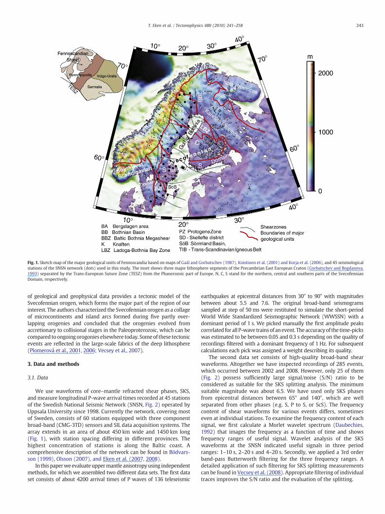
Fig. 1. Sketch map of the major geological units of Fennoscandia based on maps of Gaál and Gorbatschev (1987), Koistinen et al. (2001) and Korja et al. (2006), and 45 seismologicalstations of the SNSN network (dots) used in this study. The inset shows three major lithosphere segments of the Precambrian East European Craton (Gorbatschev and Bogdanova,1993) separated by the Trans-European Suture Zone (TESZ) from the Phanerozoic part of Europe. N, C, S stand for the northern, central and southern parts of the SvecofennianDomain, respectively.

243T. Eken et al. / Tectonophysics 480 (2010) 241–258

of geological and geophysical data provides a tectonic model of theSvecofennian orogen, which forms the major part of the region of ourinterest. The authors characterized the Svecofennian orogen as a collageof microcontinents and island arcs formed during five partly over-lapping orogenies and concluded that the orogenies evolved fromaccretionary to collisional stages in the Paleoproterozoic, which can becompared to ongoingorogonies elsewhere today. Someof these tectonicevents are reflected in the large-scale fabrics of the deep lithosphere(Plomerová et al., 2001, 2006; Vecsey et al., 2007).

3. Data and methods

3.1. Data

We use waveforms of core–mantle refracted shear phases, SKS,andmeasure longitudinal P-wave arrival times recorded at 45 stationsof the Swedish National Seismic Network (SNSN, Fig. 2) operated byUppsala University since 1998. Currently the network, covering mostof Sweden, consists of 60 stations equipped with three componentbroad-band (CMG-3TD) sensors and SIL data acquisition systems. Thearray extends in an area of about 450 km wide and 1450 km long(Fig. 1), with station spacing differing in different provinces. Thehighest concentration of stations is along the Baltic coast. Acomprehensive description of the network can be found in Bödvars-son (1999), Olsson (2007), and Eken et al. (2007, 2008).

In this paperweevaluate uppermantle anisotropyusing independentmethods, for which we assembled two different data sets. The first dataset consists of about 4200 arrival times of P waves of 136 teleseismic

earthquakes at epicentral distances from 30° to 90° with magnitudesbetween about 5.5 and 7.6. The original broad-band seismogramssampled at step of 50 ms were restituted to simulate the short-periodWorld Wide Standardized Seismographic Network (WWSSN) with adominant period of 1 s. We picked manually the first amplitude peakscorrelated for all P-wave trainsof anevent. The accuracyof the time-pickswas estimated to be between 0.05 and 0.3 s depending on the quality ofrecordings filtered with a dominant frequency of 1 Hz. For subsequentcalculations each pick was assigned a weight describing its quality.

The second data set consists of high-quality broad-band shearwaveforms. Altogether we have inspected recordings of 285 events,which occurred between 2002 and 2008. However, only 25 of them(Fig. 2) possess sufficiently large signal/noise (S/N) ratio to beconsidered as suitable for the SKS splitting analysis. The minimumsuitable magnitude was about 6.5. We have used only SKS phasesfrom epicentral distances between 65° and 140°, which are wellseparated from other phases (e.g. S, P to S, or ScS). The frequencycontent of shear waveforms for various events differs, sometimeseven at individual stations. To examine the frequency content of eachsignal, we first calculate a Morlet wavelet spectrum (Daubechies,1992) that images the frequency as a function of time and showsfrequency ranges of useful signal. Wavelet analysis of the SKSwaveforms at the SNSN indicated useful signals in three periodranges: 1–10 s, 2–20 s and 4–20 s. Secondly, we applied a 3rd orderband-pass Butterworth filtering for the three frequency ranges. Adetailed application of such filtering for SKS splitting measurementscan be found in Vecsey et al. (2008). Appropriate filtering of individualtraces improves the S/N ratio and the evaluation of the splitting.

Fig. 2. Distribution of 136 teleseismic earthquakes recorded by the SNSN (left) during 2002–2008 which were used either in P-wave anisotropy analysis (red circles) and/or in the shear-wave splitting measurement (25 earthquakes, stars).Plate boundaries are after Bird (2003). (For interpretation of the references to colour in this figure legend, the reader is referred to the web version of this article.)

244T.Eken

etal./

Tectonophysics480

(2010)241

–258

245T. Eken et al. / Tectonophysics 480 (2010) 241–258

3.2. Evaluation of shear-wave splitting

Thanks to the increasing amount of data collected during passiveseismic experiments and the development of fast computers anddifferent analysis techniques, seismic anisotropy has become a well-studied characteristic of the mantle in many regions and in differenttectonic settings (e.g., Kind et al., 1985, Vinnik et al., 1989, 1992;Babuška et al., 1993; Özalaybey and Savage, 1995; Silver, 1996;Savage, 1999; Plomerová et al., 2002, 2006, 2008a; Babuška et al.,2008).

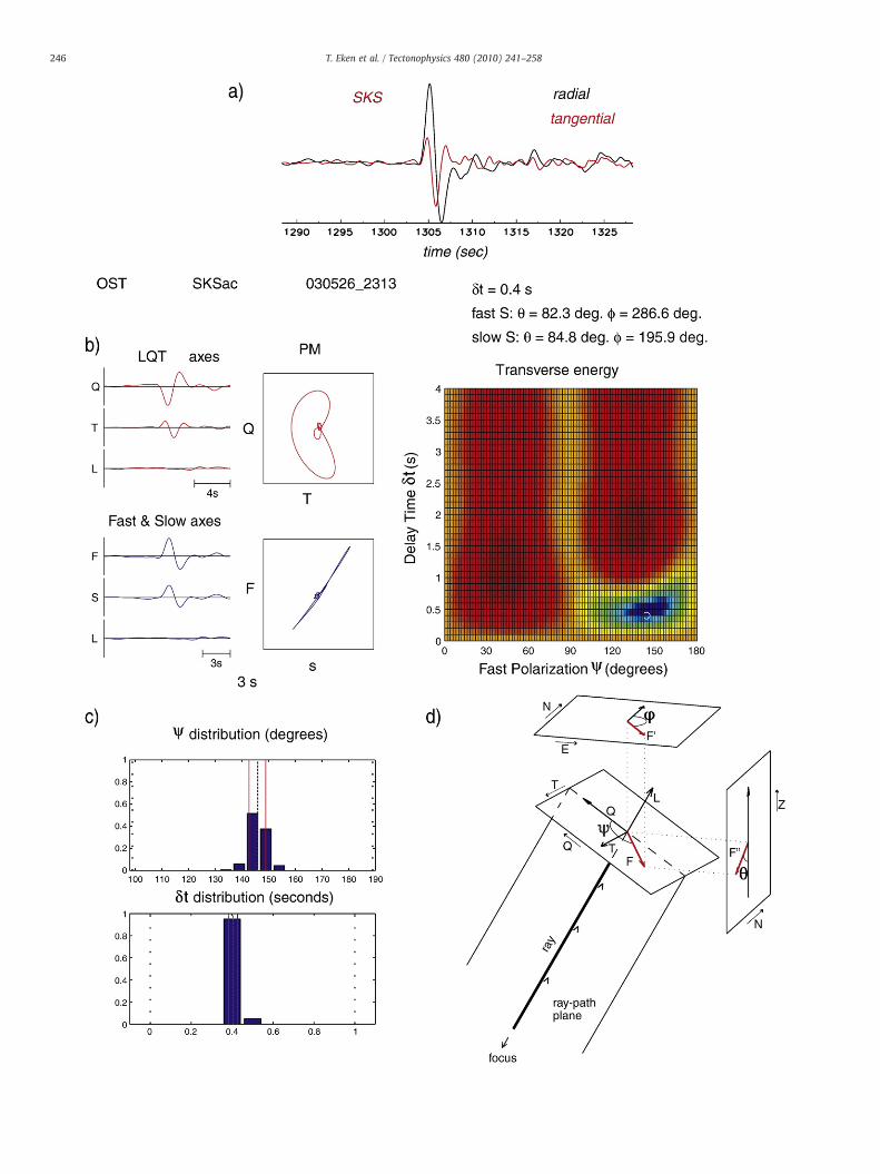
The shear-wave splitting method, first introduced by Ando et al.(1980), is based on measuring travel time delays between two splitand polarized shear waves which are generated when travellingthrough anisotropic media. This phenomenon, analogous to lightbirefringence, is one of the most common and well-establishedtechniques for studying the Earth's structure. Shear waves propagat-ing through anisotropic media split into two quasi shear waves — fastand slow. Generally, an initial short time interval of linear particlemotion will be observed corresponding to the linearly polarized fastphase. Thereafter interference between the fast and slow phasesresults in elliptical particle motion. If the original (unsplit) S-wave islinearly polarized and the waves are affected only by a zone ofconsistent anisotropy, then the recorded S-wave can be rotated suchthat two very similar phases, apart from scaling and a simple timedelay, are seen on the orthogonal components. These orthogonalphases cannot be expected to be exactly identical, because of noise,interfering phases, the effect of near-receiver structure and the effectof the free surface, but are often very similar. The orientation of theanisotropy controls the rotation angle, and the time delay betweenthe phases shows the integrated effect of the velocity anisotropy.These parameters carry information about the mineral orientation ofthe mantle material.

Various techniques are used to evaluate splitting parameters,including eigenvalue methods, transverse energy minimizationmethods and correlation approaches (Vinnik et al., 1989; Silver andChan, 1991; Savage and Silver, 1993; Levin et al., 1999). All of thesemethods are based on the idea of recovering the particle motion of theinitial shear waves, which in the case of the core–mantle refractedshear waves (e.g. SKS) is a linear radial (SV) polarization in the ray-path plane. A “correction for anisotropy” is achieved by rotatingcoordinate systems (LQT or ZRT, see below) and applying anappropriate time shift of the orthogonal polarization components(Fig. 3). Cross correlation techniques aim at detecting the maximumsimilarity between the linearly polarized fast and slow components(Iidaka and Niu, 1998; Levin et al., 1999). Another approach is a gridsearch inversion for finding the incoming polarization direction andremoving the split delay time by maximizing the aspect ratio of thecovariance matrix eigenvectors (Silver and Chan, 1988). In this studywe use the transverse energyminimizationmethod and apply it to theSKS phase, which yields more stable solutions in comparison with theother two techniques (Vecsey et al., 2008).

It is common to assume azimuthal anisotropy only and approxi-mate the anisotropic medium by symmetries with horizontal ‘fast’axes a. The splitting parameters (the fast S polarization definedby azimuth φ and delay time δt of the slow split shear wave) areevaluated in the ZRT (Z — vertical, R — radial, T — transversal)coordinate system only from the horizontal components (NS and EW)of the shear waves. The simplest forms of analysis implicitly assume avertical angle of incidence. However in reality even for steeply incidentSKS the angle of incidence is not zero and can be up to several degrees(e.g. up to 10–12° in this study). This implies the possibility ofsignificant signal on the vertical component. Taking into considerationalso a general orientation of anisotropic structures in 3D, we therefore,evaluate the splitting in the ray-parameter LQT coordinate system (L—longitudinal, Q — radial, normal to the (L–T) plane, T — transversal).This allows us to model velocity anisotropy by anisotropic media with

generally oriented symmetry axes in 3D.We evaluate the SKS splittingusing code SPLITSHEAR (Vecsey et al., 2008) based on the method ofŠílený and Plomerová (1996) which was derived from the method ofSilver and Chan (1991) and generalized into 3D.

In the 3D approach, the fast polarization direction ψ is searched forin the Q–T plane, perpendicular to the ray-path plane L–Q by takinginto consideration the incidence angle (see Fig. 3; Vecsey et al., 2008).By rotating the ray-path coordinate system by an angle ψ in the Q–Tplane and by shifting the Q and T components by the split delay timeδt, we search for the orientation of the new coordinate system inwhich the energy content of the T component is minimized. The pairof the splitting parameters (ψ, δt) is obtained as a minimum of a misfitsurface. The polarization ψ of the fast component is usually defined bytwo (Euler) angles — azimuth φ, measured from the north, andinclination θ measured from vertical upward (see Šílený andPlomerová, 1996; Vecsey et al., 2008). To evaluate the reliability ofthe splitting parameters we apply a bootstrapping technique andcalculate standard deviations σi

ang, σiδt for ψ and δt, respectively

(Sandvol and Hearn, 1994). An example of the shear-wave splittingevaluation procedure is shown in Fig 3.

3.3. Evaluation of P-residual spheres

The shear-wave splitting parameters (ψ and δt) are generallyaccepted as a measure of seismic anisotropy. However, the structureof the upper mantle is often more complicated than can be describedby a single anisotropic layer with a horizontal ‘fast’ symmetry axis.Using only shear-wave data to analyse other orientations ofanisotropy can be difficult. Especially for SKS data there is a limitedrange of incidence angles and often also limited ranges of availablebackazimuths because of the distribution of suitable sources. Limitedray-path coverage means that the splittings themselves are generallyinsufficient to allow retrieval of the 3-D orientation of the structures,even if the Earth were laterally homogeneous and had a singleorientation of anisotropy. To some extent, this can be improved byincluding more data with a better geographical distribution of foci.However, as the method requires signals with good signal-to-noiseratio which can be obtained only from large events (M>∼6.5) thenumber of such events available remains limited.

Aswell as affecting shear-wave propagation, seismic anisotropy alsoaffects propagation of P waves, for which a much better geographicaldistribution of foci is available compared to SKS. Moreover, measuringfirst arrival times of the P waves is often feasible for lower-magnitudeevents than those suitable for SKS splitting analysis. Though P wavescarry primarily information about velocity heterogeneities, effects dueto a directional dependence of velocities (anisotropy) can be extractedas well. Babuška et al. (1984) introduced an analysis of the pattern ofrelative P travel time residuals plotted in a lower hemisphere projection(P spheres) as a function of back azimuth and angle of upward propa-gation (‘incidence’) within the upper mantle.

The trade-off between the heterogeneity and anisotropy effectsexisting in the P residuals can create difficulties and must be takeninto account. Travel time perturbations due to variations of thicknessof the crust and sediments and their average velocities beneathindividual stations are minimized by calculating station correctionsfor each ray. Effects from the deep mantle and focal areas are reducedby normalization, i.e. by calculating P residuals relative to a referencelevel which for each event is the mean residual computed either fromresiduals of a set of high-quality well distributed reference stations orfrom residuals of all stations of the array.

The P spheres are constructed for each station and show directionalterms of relative residuals. The directional terms are calculated fromrelative residuals at a station by subtracting a directional mean of thestation, obtained by two-parameter filtering the relative residuals ateach station. The method thus decomposes the observed arrival timeresiduals into an isotropic part anddirectionally dependent components

246 T. Eken et al. / Tectonophysics 480 (2010) 241–258

247T. Eken et al. / Tectonophysics 480 (2010) 241–258

(Babuška and Plomerová, 1992). This allows us to compare easily thedirectional components at different stations, while constant time delaysrelated to e.g. different average velocity beneath the stations do notaffect the images. Spatially varying smoothed directional terms areshown in a lower hemisphere stereographic projection as a function ofazimuth and angle of propagation (measured from the vertical) withinthe mantle lithosphere. In general, positive residuals in P spheres(relatively delayed arrivals) indicate low-velocity directions of propa-gation, while negative values (relatively earlier arrivals) reflect high-velocity directions. The anisotropic pattern extracted from the P spherescan reveal consistent fabrics of individual lithosphere domains overlarge continental provinces (Plomerová et al., 2001, 2002, 2006;Babuška and Plomerová, 2006; Babuška et al., 2008). Directionalvariations of P-wave velocities, evaluated from the P spheres, providecomplementary information to shear-wave splitting studies.

3.4. Modelling anisotropic structure — joint inversion

Most anisotropic modelling is based on an assumption of homoge-neous anisotropy within individual domains in the upper mantleoverlying the sub-lithospheric mantle. However, there are differentapproaches for retrieving information about upper mantle anisotropicstructure. Themost common approach deals with azimuthal anisotropyonly, while more sophisticated methods solve the problem in 3D, i.e.allowing for an arbitrary orientation of the axes of anisotropy (Babuškaet al., 1993; Šílený and Plomerová, 1996). Considering a generalorientation of the symmetry axes in 3D and modelling of twoindependent observables of anisotropy (shear-wave splitting and Pspheres) influence also our choice of model peridotite aggregates. Weleave the simple search for azimuth of the fast axis a, of either hexagonalor orthorhombic symmetry in the horizontal plane, and instead wesearch for the general orientation of such aggregates. The form ofanisotropywithin the Earth could, of course, bemore complex than oneof these two ideal cases. However, when dealing with real data, we arelimited in the number of observed rays sampling the structure,dependent upon the location of observed teleseismic events. This,together with other complications such as external noise and localscattering effects, means that it is not possible to invert for e.g. the fullanisotropic tensor, and choose to limit our attention to the two idealisedcases of aggregates with hexagonal or orthorhombic symmetries. Thisdoes not imply thatwebelieve thatmantle anisotropymust always haveone of these two structures, but that in many geographical areas one ofthese forms of anisotropy will be dominant. If so, the combinedinformation content of shear-wave splitting and P-wave arrival timeperturbations can distinguish between the two cases, given sufficientdata and that our basic assumptions, such as that there are not multiplezones of anisotropy with different orientations below the station, arevalid. Modelling anisotropy independently for P- and S-wave aniso-tropic parametersmaynot provideunique solutions as to the symmetry.However, because the P- and S-wavedata are sensitive to the anisotropyin differentways, joint inversion/analysis is better suited to inferring thetype and orientation of the symmetry of each upper mantle domain.Seeming discrepancies between the high-velocity directions derivedfrom the P-wave anisotropic parameters and average azimuths of thefast SKS phases if interpreted in 2Dmay be removed in the 3D approachallowing symmetries with inclined axes, representing either dippinglineation a (orthorhombic or a-axis hexagonal models) or dipping the(a,c) foliations (b-axis hexagonal models).

Šílený and Plomerová (1996) proposed an inversion algorithm forshear-wave splitting parameters to retrieve information aboutanisotropic structure within the continental mantle lithosphere with

Fig. 3. Example of shear-wave splitting evaluation. a) Radial and transverse components of SKS6.9 Mw and epicentral distance 92.3°; b) particle motions (PMs), misfit function and splitting pestimates of the evaluated splitting parameters by the bootstrap method (Sandvol and Hearn,splitting measurements (Šílený and Plomerová, 1996). (For interpretation of the references to

generally oriented symmetry axes in 3D by taking into account theangle of incidence and the direction of propagation of arriving waves.This approach was extended by including observables on anisotropyextracted from P-wave travel time deviations and has been usedsuccessfully to study fabrics of the mantle lithosphere in severalcontinental regions (Plomerová et al., 1996, 2001, 2002, 2006; Babuškaand Plomerová, 2006; Babuška et al., 2008). Joint analysis of P and Sdata has the potential to reduce some of the ambiguities and seeminginconsistencies (Babuška et al., 1993; Fouch and Rondenay, 2006;Babuška et al., 2008) in modelling anisotropy within the mantle.

The natural way to invert jointly both the shear-wave splittingparameters and the directional terms of relative P residuals is tominimize the misfit function,

F = ∑M

i=1

jδtobsi −δtij2ðσδt

i Þ2

264

375 + ∑

M

i=1

jψobsi −ψij2ðσang

i Þ2

264

375 + ∑

N

j=1

jΔtobsj −Δtjj2ðσΔt

j Þ2

264

375;

ð1Þ

where Δt(θ,φ,H,α), ψ(θ,φ,H,α) and δt(θ,φ,H,α) represent syntheticcalculations of anisotropy-related terms in the relative P residuals(Δt), and the fast S polarization (ψ) and the split delay time (δt). Theupper index ‘obs’ stands for observed values. Angles θ (inclinationfrom the vertical) and ϕ (azimuth) are the angles which define theorientation of the symmetry axis of a model aggregate of thickness H.M is the number of observed ψ and δt while N is the same for Δt.Strength of anisotropy and symmetry are defined by parameter α. Weassume two hexagonal symmetries with either the ‘slow’ b axis andhigh-velocity foliation plane (a,c) or with the ‘fast’ a lineation andlow-velocity plane (b,c), as an approximation of a peridotite aggregatewith orthorhombic symmetry (Babuška et al., 1993).

The aggregates with ‘slow’ symmetry axes can represent originallyoceanic lithosphere that lies over unstable sub-lithospheric mantleflow. Aggregates with a ‘fast’ symmetry axis can be considered as anapproximation of orthorhombic aggregate with the high-a, low-b andintermediate-velocity c axes of symmetry. Values σi

ang, σiδt and σj

Δt arestandard deviations of ψi, δti and Δtj. We approximate the large-scaleanisotropy of the upper mantle by peridotite aggregates with elastictensors derived from data from mantle xenoliths (Christensen, 1984;Nicolas and Christensen, 1987; Babuška and Cara, 1991; Babuška et al.,1993; Ben Ismail and Mainprice, 1998). Strength of anisotropy of themodel aggregates used are kP=5.4% and kS=4.8% in case of the b-axis mode, and kP=8.2% and kS=3.4% in case of the a-axis model.

The three data sets entering Eq. (1) are different in character, andthe simple weighted summation of misfits may not be the optimalmethod for solving the inverse problem. Following Kozlovskaya et al.(2007) we apply a multi-objective optimization (MOP) procedure.The misfit function is decomposed into its components

f1 = ∑M

i=1

jδtobsi −δtij2ðσδt

i Þ2

264

375; f2 = ∑

M

i=1

jψobsi −ψij2ðσang

i Þ2

264

375; f3 = ∑

N

j=1

jΔtobsj −Δtjj2ðσΔt

j Þ2

264

375

ð2Þ

The global minimization for the inverse problem is based on asearch for a set of Pareto optimal solutions or trade-off solutions in thespace of misfit functions (see Kozlovskaya et al., 2007). This approachalso allows us to combine solutions of individual pairs of misfitfunctions or use a minimum of a single one.

phase recorded at the station OST from an earthquake of 20030526-2313withmagnitudearameters from the transverse energyminimizationmethod (Vecsey et al., 2008); c) error1994); d) schematic illustration of the LQT coordinate system and angles used in the SKScolour in this figure legend, the reader is referred to the web version of this article.)

248 T. Eken et al. / Tectonophysics 480 (2010) 241–258

4. Body-wave anisotropy in the mantle beneath the SNSN

4.1. Shear-wave splitting measurements

In accordance with themost commonly used presentation of resultsof shear-wave splitting analyseswe show (Fig. 4) average azimuthsφ ofthe fast S polarization (considering the full 0–360° interval) and the splitdelay times δt for all stations of the SNSN array along with standarddeviations (SD)of themeans.Due tovariations of single pairs of splittingparameters at each station and the distribution of foci (Fig. 2), whichform two main geographical groups, we calculated at each station theaverage values for waves approaching the SNSN stations from thewestern and eastern back azimuths separately. At some stations (SAL,

Fig. 4. Average fast S polarization azimuths φ and split delay times δt calculated at each staFig. 2) along with standard deviations (STDs).

LAN, UDD, BUR, ROT), we present the splitting parameters only for onegroup of events owing to the lack of recorded signals from the oppositeside, or for a single measurement (e.g., UDD, FAL DUN) for the samereason.

The fast S polarizations of waves from the west and east differ atmost of stations and the differences exceed the SD range (Fig. 6a–c).Different polarisations at different stations also demonstrate lateralvariations in anisotropy. Usually, neighbouring stations exhibit similarpolarizations, but lateral variations along the SNSN are obvious. Formapping the lateral variations we divided the SNSN stations into 4groups according to the character of their polarizations. From thepoint of view of azimuthal anisotropy (azimuth±180°), a NE–SWtrend of the polarization azimuth prevails in the northern part of the

tion separately for waves arriving from (a) western and (b) eastern backazimuths (see

249T. Eken et al. / Tectonophysics 480 (2010) 241–258

shield (Region 1, north of 65° N). To the south (Region 2, 62–65°N) thepolarizations rotate to about E–W, whereas NW–SE polarizationsdominate south of 58° N (Region 4). Scattered orientations ofpolarizations with many null splits are typical for Region 3 (between∼58 and 62° N). Splitting at three stations located on the sea shore(HEM, NYN, BYX, Fig. 4) deviate from the general trend of polarizationmeasured at nearby stations. Possible errors of seismometer mis-orientation or a wrong polarity were checked and excluded as asource of the deviations. Because all the events could not be evaluatedat each station of the SNSN, which might affect to some degree theaverage values, we show the geographic variation of evaluatedsplitting using an example of a single shear wave approaching theSNSN from the ∼E (i.e., the epicentral distance does not change muchalong the array). Ellipses of the initial particle motions (Fig. 5a) arenarrow for this event, allowing mapping the four regions. Evaluated

Fig. 5. (a) Lateral variations of particle motion (PM) of the SKS phase shown in the Q–T plane20070808-1705 with backazimuth 94° and epicentral distance 94.3° relative to the centre oshow the fast polarization azimuths φ and split times δt of the SKS phase. Four regions with(see also Fig. 4 with average splitting parameters). (For interpretation of the references to

polarizations (Fig. 5b) for this direction of propagation point to theSW (Region 1) and to aboutW (Region 2), nulls dominate in Region 3,while polarizations to the NW characterize Region 4 in the south. Theindividual regions exhibit not only different mean values of thesplitting parameters, but also different characteristic distributions ofindividual values within the regions (Fig. 6).We illustrate variations ofthe fast shear-wave polarizations within each of the four groups inrose diagrams (Fig. 6a). To increase visibility of the differences and tobe compatible with commonly used presentations, we added into thediagrams also opposite azimuths (φ+180°, light colours). Differencesin scatter of the polarization directions are immediately clear (Fig. 6a),both among the groups and between propagations from the west andfrom the east. Region 1E (easterly back azimuths), Region 3 W(westerly back azimuths) and Region 4E show distinct prevailingazimuths of polarizations, but clearly different one from polarizations

(the Q axis pointing to backazimuth) at stations of the SNSN array from a single event off the SNSN. (b) Lateral variations of evaluated splitting parameters across the array. Wesimilar anisotropic signal expressed in shear-wave splitting characteristics are colouredcolour in this figure legend, the reader is referred to the web version of this article.)

250 T. Eken et al. / Tectonophysics 480 (2010) 241–258

from opposite directions (1 W, 3E, 4 W). Polarizations of wavesarriving from the west for Region 1 W and Region 4 W show twodominant azimuth values which roughly differ by ∼40° but neither isidentical with the two significant azimuths for propagation from theeast (Region 1E and Region 4E). Similarly, Region 3E which has thegreatest number of measurements differs from that of signals arrivingfrom the west, but the largest scatter is characteristic for sites in thisgroup. Though the dominant direction of polarization in Region 2 isidentical for signals from the east and from the west, the scatter of thepolarization azimuths is much larger for propagation from the west;similar to what is observed in Regions 1 W and 4 W. Only in Region 3,with many nulls, is the scatter of polarization azimuths larger forwaves arriving from the E than from the W. Split delay times whichare up to 2 s and polarization azimuths evaluated at individualstations as a function of back azimuth are presented in Fig. 6b and c

Fig. 6. Splitting parameters at stations of SNSN grouped into four sub-regions: (a) rose diagramshown with their weighted mean and standard deviations for four different regions and (c)phases, and (d) histogram of all measured split delay times. (For interpretation of the referenc

along with their SD. Split delay times less than 0.2 s are considered asnulls and they are not plotted. The mean delay time of 223 slow splitshear-wave measurements is 0.91±0.19 s (Fig. 6d).

4.2. P-wave anisotropy observations

We have sufficient data to construct reliable P-residual spheres forall stations of the SNSN, which allowed us to infer velocity variationsbeneath each of them as a function of the direction of wavepropagation. The stations in the northernmost part of the arrayrecorded fewer events, because the SNSN arraywas installed graduallyfrom the south. However, even the northern stations recorded enoughP arrivals for first estimates of velocity variations. The directionalterms of the relative residuals are small (−0.5<Ri,k<0.5 s), but theydo show systematic dependence on back azimuth. Most of the stations

s of the fast shear-wave polarization azimuths, (b) individual split delay timeswhich arethe fast shear-wave polarization azimuths as a function of backazimuth of arriving SKSes to colour in this figure legend, the reader is referred to theweb version of this article.)

Fig. 6 (continued).

251T. Eken et al. / Tectonophysics 480 (2010) 241–258

Fig. 6 (continued).

Fig. 7. Stations of the SNSN grouped according to their P-sphere type and examples oftypical P spheres for each group. Colours of the station symbols and the outer circles ofthe spheres are identical. The spheres show azimuth-incidence angle dependent termsof relative residuals related to anisotropy. Negative terms (blue) mark relatively high-velocity directions of propagation, whereas positive terms (red) correspond to low-velocity directions relative to an isotropic mean velocity beneath each station. Dashedcurves indicate boundaries between the mantle lithosphere domains with similar fabricseen by the P waves.

252 T. Eken et al. / Tectonophysics 480 (2010) 241–258

exhibit ‘bipolar patterns,’ with negative and positive residualsconsistently in separate halves of the lower hemisphere projectionThis means that waves approach a station from one side faster(negative residuals) thanwaves from the other side (positive residualsin the spheres), relatively to an isotropic velocitymean (the directionalmean) beneath each station. We inspected visually the P-residualspheres and according to their patterns we divided the stations intofive groups. Stations were ordered alphabetically for this ‘typeanalysis,’ which prevented a subjective view in the pattern-typeclassification. A map view of the P-sphere types (Fig. 7) shows thatnearby stationswere usually assigned to the same class. Stationswith asimilar residual pattern in the P spheres form geographical groupsindicating a regional dependence of P-velocity anisotropy. Negativeresiduals for waves from the N–E are typical at four stations in thesouth and most of stations in the central part of the array (yellowstations in Fig. 7). Between these two regions, the pattern suddenlyflips over (see turquoise stations in Fig. 7). Further to the north, earlyarrivals dominate for WSW–N azimuths (green stations). Station GOTononeof the islands in the south, shows a similar pattern. Four stations(two pairs, purple in Fig. 7) are anomalous. Station OSK is typical forthese stations and shows a rotation by about 90° of the pattern relativeto stations in the neighbouring areas.

Apart from the distinct bipolar patterns described above, severalstations do not show any systematic variation of the residuals withback azimuth (black triangles, Fig. 7). Such behaviour is observed atsome stations around 59–60°N along the coast in themiddle part of thearray. The residual pattern at the northernmost group of stations (greystations in Fig. 7) does not have the ‘bipolar character,’ but the residualdistribution is not random. The negative and positive residuals con-centrate into quadrants (Fig. 7).

Another manifestation of directional variations of P velocity isshown in Fig. 8, where the average directional terms are calculated in60° azimuth bins. In the first step, we determined at each station theazimuth which divides the positive and negative half of the P sphere,i.e., the azimuth of the strike of the ‘bipolar pattern.’ This azimuthrepresents the starting point for setting the 60° intervals, in which wecalculate the averages. Having three azimuth bins per negative half ofthe sphere and other three bins per positive half with their individualstarting angles, assures a smoothing of the observables withoutmasking directionswith extremes. In case of stationswithout a distinctbipolar pattern we calculated the averages in quadrants (90° bins).Grouping the stations according to visual inspection of patterns of theP spheres (Fig. 7) was managed based on the consistent orientation of

directions of relatively higher or lower velocities for each station. Thecharacteristics of groups changeswhen crossing from one boundary toanother (Fig. 8).

5. Joint inversion of body-wave anisotropic parameters

To model the anisotropic fabric of several mantle domainssegregated beneath the SNSN we initially inverted the P spheres atgroups of stations as defined in Fig. 7 (see also Table 1). Stations withno patternwere not included in the inversion. Station EKS sitting closeto a domain boundary exhibits the clear P-sphere pattern observed atthe southernmost stations (yellow triangles in Fig. 7), but amplitudesin the spheres are much lower than those at stations within thesouthern block. Therefore, the station was not included into data ofthe group in the south. Models with plunging symmetry axes (misfitf3 solutions in Table 2), both with the ‘fast’ and ‘slow’ b axes — mimic

Fig. 8. Directional terms of the relative P residuals averaged in the 60° azimuth bins, incases with a ‘bipolar pattern’ of the P spheres (for more details see the text), otherwisein 90° azimuth bins. Grouping of the stations is the same as in Fig. 7. Size of the fullarrows corresponds to the bin averaged relative delays (positive directional terms —

red) or early arrivals (negative directional terms — blue), see the scale in the lowerright. Large dashed arrows mark schematically azimuths of ‘slow’ b symmetry axes ofhexagonal models with dipping (a,c) foliation which fit the observations, as one ofpossible models. (For interpretation of the references to colour in this figure legend, thereader is referred to the web version of this article.)

Table 1Grouping of stations.

Group1: N. Svecofennian-KarelianP (grey triangles, Fig. 7): NIK, KUR, LAN, MAS, PAJ, SAL, DUN, ERTSKS: NIK, KUR, LAN, MAS, PAJ, SAL, DUN (from W only)

Group 2: N. SvecofennianP (green triangles): SJU, LIL, BURSKS: SJU, LIL, BRE (from E), UMA (from E)

Group 3: C. SvecofennianP: (yellow triangles): NOR, SOL, BRE, UMA, HEM, ROTSKS: NOR, SOL, HAS, ROT, UMA (from W), BRE (from W),

ARN (from E), IGG (from E), OST (from E)

Group 4: S. SvecofennianP (blue triangles): NRA, ASK, LNK, VST, IGG, GRA, FLY, UP1, AALGroup 4a — northSKS: ASK, ESK, NRA, BAC, UP1, FLY, AAL, NRT (from W), GRA

(from W)Group 4b — southSKS: VST, BYX (from E), EKS (from E), LNK (from E), VIK

(from E)

Group 5: TIBP (yellow triangles): DEL, BLE, VXJSKS: DEL, BLE, VXJ, OSK (from W)

253T. Eken et al. / Tectonophysics 480 (2010) 241–258

well the observed anisotropic signals. While the high-velocityfoliation (a,c) in the b-axis models or lineation a in the a-axis modelsdip to the NE in the southern and central parts of the region, they areoriented with approximately opposite azimuths in the south-centraland south-north parts— they dip to the SW and NW, respectively. It isdifficult to decide only from inversion of P spheres which of thesymmetries approximate the fabric better, because minima of themisfit functions are very close to each other. However, mutualorientation of the average fast S polarization azimuths and dippingaxes of the a- or b-models allows us to judge which of the modelsretrieved from the P-sphere inversions better approximates the fabricof the mantle lithosphere (Šílený and Plomerová, 1996). The averageφ parallels the a axis in the a-model, whereas they parallel the strikesof dipping (a,c) foliation in the b-model. In our observations theaverage fast polarization azimuths mostly parallel the strikes of the b-models, which implies that models with dipping (a,c) foliations seemto be more suitable for the lithosphere beneath the SNSN.

In the second step we inverted the shear-wave splitting para-meters and performed joint inversion of body-wave anisotropicparameters with all possible combinations of misfit functions f1, f2and f3 and isotropic velocities of the models in range of 8.0–8.5 km/s.In Table 2 we present only stable solutions which satisfy theindependent P- and S-wave information in the data. Criteria ofstability were small differences between results from a summation ofmisfit functions and optimum Pareto optimum solutions, as well asthe lowest values of misfit functions in the inversion outputs. Resultsof the joint inversion (Pareto optimal solutions) confirm the b-axismodels as the most suitable approximation of the anisotropicstructure of individual mantle lithosphere domains (see Fig. 11)with only one exception (small Group 4 — North Svecofennian, seealso Table 1). Model thicknesses of most of the stable solutions,assuming the model strength of anisotropy, are close to thethicknesses of the mantle lithosphere domains (Table 2) calculatedas mean values from a model of the lithosphere thickness (Plomerováet al., 2008a,b) after subtracting appropriate crust thicknesses (Olssonet al., 2008).

6. Discussion

The ubiquitous trade-off between the intensity of velocity aniso-tropy and the corresponding volume of the anisotropic medium isparticularly significant when analysing SKS data. In principle, thesource of the SKS splitting can be located anywhere along the ray pathbetween the core–mantle boundary and the receiver. To locate theanisotropic volume, we have to rely on indirect indications derivedfrom, e.g., calculating the Fresnel zones in case of array data, or,combining different methods and observables (e.g., Babuška et al.,1993, 2008; Fouch and Rondenay, 2006 for a review). However,shear–wave splitting evaluated for P to S phases converted at the 410discontinuity (Olsson, 2007) allows us to associate the anisotropywith the upper mantle structure above the discontinuity. Meandifferences between the fast S polarization azimuths from splitting ofSKS and P410s phases, and between the corresponding split delaytimes are 30° and 0.3 s, respectively, excluding sites with null splitsfrom either method (Fig. 9). We found a correlation coefficient of∼0.82 for the distribution of fast polarization azimuths evaluated fromSKS and P410S phases after a regression analysis. The 95% confidenceinterval of the average difference in azimuth is rather broad

Table 2Joint inversion of body-wave anisotropic parameters — Pareto optimum solutions.

Region ‘Slow’ b axis ‘Fast’ (a,c) foliation H viso ‘Fast’ a lineation H Viso HML

φ θ φd α(km) (km/s)

φ θ(km) (km/s) (km)

Group 5: South TIBf3 215 55 35 55 110 8.29 50 30 70 8.49 130F= f2+ f3 215 45 35 45 100 8.23 – – – – 130F= f1+ f2+ f3 215 65 35 65 130 8.34 – – – – 130

Group 4: South Svecofennianf3 40 25 220 25 50 8.07 205 15 50 8.50 125F= f2+ f3 (4a) 340 20 160 20 50 8.10 – – – – 130F= f2+ f3 (4b) 45 45 225 45 50 8.14 – – – – 115F= f1+ f2+ f3 (4a) 340 20 160 20 60 8.10 – – – – 130F= f1+ f2+ f3 (4b) 40 80 220 25 70 8.35 – – – – 115

Group 3: Central Svecofennianf3 210 35 30 35 60 8.19 30 70 50 8.17 115F= f2+ f3 210 30 30 30 60 8.16 – – – – 115F= f1+ f2+ f3 205 70 25 70 110 8.37 – – – – 115

Group 2: North Svecofennianf3 85 40 265 40 60 8.17 300 70 70 8.17 105F= f2+ f3 – – – – – – 250 20 50 8.51 105F= f1+ f2+ f3 – – – – – – 255 70 90 8.14 105

Group 1: North Svecofennian-Karelianf3 55 85 235 85 90 8.37 310 85 130 8.10 100F= f2+ f3 325 30 145 30 50 8.17 – – – – 100F= f1+ f2+ f3 325 55 145 55 50 8.32 – – – – 100

Azimuth φ and inclination θ (measured from vertical upward) are Euler angles defining the symmetry axis; φd and α are dip-azimuth and inclination of the (a,c) foliation plane ofolivine aggregate (inclination measured from horizontal downward); H is thickness of the anisotropic medium; HML is thickness of mantle lithosphere according to Plomerová et al.(2008a,b). Numbers in bold are preferred orientations in case of less stable solutions.

254 T. Eken et al. / Tectonophysics 480 (2010) 241–258

(30°±44°), but the average values of both measurements areinfluenced by the distributions of events, from which waves arrivewith different ranges of back azimuths and incidence angles.Therefore, the averages do not differ only due to measurement errors,but as a result of sampling themantle structures by different rays withdifferent (φ, i) of both sets. Even for the same backazimuths theincidence angles (i) of the P410s converted phases are less steep thenthose of the SKS. Vecsey et al. (2007) document even differences infast S polarizations between the SKS and SKKS phases from one event,arriving thus from the same backazimuth but with different incidenceangles, if waves propagate through structures with non horizontal aaxis. All these aspects affect results regarding azimuthal anisotropy,both the average fast S polarization azimuths and the apparent splitdelay times, particularly in regions where axes of anisotropy plunge. Acertain role can be attributed to the frequency dependence of thephenomenon as well. Nevertheless, at most sites we have foundsimilar polarizations of the shear waves, particularly in the southernand northern part of the SNSN array, while larger deviationsconcentrate in the central part (mostly in the southern Svecofennian,Figs. 5b, 6b), with complicated structure and large scatter of the SKSsplitting measurements (Fig. 6a), which reduces the correlation ofboth sets of independent measurements.

One possible explanation of upper mantle anisotropy is a flow inthe sub-lithospheric mantle (e.g., Vinnik et al., 1989; Long and Silver,2008). In case of lithospheric roots (cratonic keels) anisotropy may beassociated with asthenospheric flow around the lithospheric thick-ening (Bormann et al., 1996; Wylegalla et al., 1999; Pedersen et al.,2006). In the central part of Fennoscandia the lithosphere–astheno-sphere boundary sinks to depths of about 200 km (Plomerová et al.,2008b). If sub-lithospheric in origin, the upper mantle anisotropy willthen be located between 200 km and 410 km, considering thevsplitting from the P to S converted waves (Olsson, 2007). However,Plomerová et al. (2006) and Vecsey et al. (2007) modelled theanisotropy and its changes observed in south-central Fennoscandia(SVEKALAPKO array, Finland) by a domain-like structure of theanisotropic mantle lithosphere. Similarly, orientations of the fast S

polarizations, pointing on average towards the lithosphere thickening(Plomerová et al., 2008b) as well as distinct directional and geographicvariations (e.g. Fig. 6), do not support the ‘flow-around’model beneaththe SNSN.

Tomographic images of velocity perturbations calculated sepa-rately from SH and SV arrivals evaluated at the SNSN differ down toabout 200 km (Eken et al., 2008). Below this depth, the perturbationsare comparable on the large scale. The discrepancy between the SH-and SV-tomography results locate, independently of the othermethods, the source of the observed anisotropy into the upper200 km of the upper mantle occupied mostly by the mantlelithosphere. Therefore, instead of the ‘flow-around’ model, we searchfor 3D self-consistent anisotropic models of the upper 200 km of themantle, which are compatible for independent observations (shear-wave splitting, P-wave anisotropy).

There are several indications why we associate the observedanisotropy with mantle structure: size of the structures in relation towavelength of teleseismicwaves, themagnitude of the split delay times,and correlation of the domains identified with results from mantletomography. Both the tomographic images and P410s converted waveslocate the anisotropy within the upper 200 or 400 km, respectively.Average split delay time is∼1.2 s (Fig. 6b),which substantially exceeds agenerally accepted value of 0.3 s for the split delay time caused byanisotropy of the crust (see Barruol and Mainprice, 1993).

Distinct lateral variations of anisotropic parameters, characterizedby a steady anisotropic signal within each region and its suddenchange at boundaries of tectonic units (see Fig. 1), support the ideathat the important source of the observed variable anisotropy has tobe associated with the structure of the mantle lithosphere. If theanisotropy were confined only to within the sub-lithospheric part ofthe upper mantle and related to ongoing mantle flow, smooth large-scale changes of anisotropic parameters should dominate, but this isnot observed. Instead, there are abrupt changes between clearlydelimited areas of consistent anisotropic patterns expressed both inthe shear-wave splitting and in the P spheres, which we interpret by adomain-like structure of the mantle lithosphere.

Fig. 9. Average fast shear-wave polarizations (azimuths and delay times) evaluatedfrom SKS phases (this paper) and from P410s phases (P- S-waves converted at 410 kmdiscontinuity; Olsson, 2007). In this comparison, the SKS splitting parameters wererecalculated into the 0–180° azimuth range to be compatible with results from P410sphases. Correlation between splitting parameters for the two different types of shearphases locates the source of the anisotropy above 410 km. (For interpretation of thereferences to colour in this figure legend, the reader is referred to the web version ofthis article.)

255T. Eken et al. / Tectonophysics 480 (2010) 241–258

To understand better the structural zoning of the region beneaththe SNSNwe superimpose the zones determined from the shear-wavesplitting and from the P-wave anisotropy onto velocity perturbationimages from the P, SH, SV and SH–SV differential tomography (Ekenet al., 2007, 2008) in slices at 150 km depth (Fig. 10). After comparingimages obtained from all layers in the upper mantle down to 260 km,we chose these slices at 150 km as representative of perturbations inthe mantle lithosphere in all tomography images for the four differentcases. The boundaries of the anisotropic domains correlate withboundaries between the large high- and low-velocity heterogeneitiesin the mantle. However, the anisotropic pattern cannot be explainedas an artefact produced by the heterogeneities. The P-residual patternof some of the southern stations (Region 4, with high velocities to the

NE) could be partly associated with the high-velocity heterogeneitybeneath Region 3, but the P pattern in the blue group (Region 3) isexactly opposite to that expected if it were due to high-velocityheterogeneity related to the lithospheric thickening. Moreover, wefound similar zoning in the geographical variations of the shear-wavesplitting parameters, which can hardly be associated with isotropicvelocity heterogeneities only. Similarly, boundaries between groupsof stations with consistent anisotropic patterns in the P spheres incentral Sweden at about∼61° N and further to the north at about∼65°N are close to the boundaries between the high- and low-velocityperturbations of the tomography images. However, there is only alittle, if any, relation between the anisotropic velocity manifestationand potential effects of the heterogeneities on the P spheres.

Similarly to several other continental regions (e.g., Babuška andPlomerová, 2006) anisotropy of individual mantle lithospheredomains beneath Sweden is approximated, with only one exception,by hexagonal aggregates with ‘slow’ symmetry axis b and dippinghigh-velocity (a,c) foliations. This symmetry fits both the P-waveanisotropic parameters (P spheres) and variations of SKS splitting independence on direction of propagation within a domain. Thedirectional variations of evaluated fast S polarizations at a group ofstations (Fig. 6a) clearly justify symmetry with dipping axes derivedfrom the P spheres and demonstrate the necessity of applying the 3Dapproach of modelling anisotropic structures of the mantle domainswith generally oriented symmetry axes.

Boundaries of the domains correlate with themain crustal terranesalong the Swedish coast of Fennoscandia: the Karelian province in theNorth, the northern, central and southern Svecofennian provinces andthe Trans-Scandinavian belt in the South, covered by the seismicstations of the SNSN. The crustal terranes reflect accretionary andcontinent–continent collisional processes acting during formation ofFennoscandia. The southernmost domain of the mantle lithosphere(ML) is geographically situated mostly beneath the southern part ofthe TIB. The ML fabric characterized by high velocities dipping to theNE is the same as retrieved in another anisotropy study along the TORarray for stations north of the ST part of the TESZ located in theSveconorwegian (Southwest Scandinavian) domain (Plomerová et al.,2002). We found weak or no anisotropy at stations north of 58° Nalong the coast of the South Svecofennian domain (Figs. 5 and 7)much like in the shear-wave splitting study byWylegalla et al. (1999)and by Plomerová et al. (2002), a study including a joint interpreta-tion of body-wave anisotropy. Variable fabrics along about 60° N fromthe east to west are similar to that found and modelled in Plomerováet al. (2001). On the other hand, the region beneath the TIB and SouthSvecofennian province represents the most complex structure of theregion. The integrated character of P-wave propagation and theshorter wave length compared with shear waves allows us to retrieveaverage lithospheric structure (Fig. 11, model with dashed ring), withthe high-velocity foliations dipping to the SW. Wavelengths of shearwaves are about four times larger than those of P waves. Therefore,the split shear waves can ‘see’ only larger structures. Joint inversion ofanisotropic observables at a group of inland stations (Group 4b) resultin a model similar to that derived from P waves (Fig. 11, Table 2). Thesolution of the joint inversion for stations forming Group 4a (Table 1,Fig. 11) is slightly rotated. Measurements at stations of the groupcontain many small split delay times, nulls and variable orientationsof the fast polarizations (see also Fig. 5a), and reflect real/apparentlower anisotropy or a collage of several smaller blocks. The anisotropyobserved in the Bergslagen area reflects its very complicated tectonicdevelopment, multistage lithosphere growth and crustal reworkingof this classical ore district of the southern Svecofennian domain(Andersson et al., 2006). There is no stable solution of the jointinversion for the whole of Group 4.

Further to the north, in the Central Svecofennian domain (north of∼61° N), the ML fabric changes and the fast velocities plunge to theNE. According to observations at three stations on the coast the fabric

Fig. 10. Velocity perturbation images from the P, SH, SV and SH–SV differential tomography (Eken et al., 2007, 2008) in slices at 150 km depth superimposed with the anisotropic zones determined from the shear-wave splitting and from theP-wave anisotropy (this study). The boundaries of the anisotropic domains (green) correlate with boundaries between the large high- and low-velocity heterogeneities in the mantle and document the domain-like structure of the mantlelithosphere beneath Fennoscandia.

256T.Eken

etal./

Tectonophysics480

(2010)241

–258

Fig. 11. 3D self-consistent anisotropic models of individual mantle lithosphere domainsderived by joint inversion of body-wave anisotropic parameters (see Table 2). Unstablesolution for the South Svecofennian is with dashed contour and solutions for the twosub-regions are shown as well. Boundaries of the domains (dashed green) correlatewith those of major crustal terranes (orange curves). The mantle lithosphere domainsof the Proterozoic part of Fennoscandia beneath the SNSN seem to be sharply boundedand separated by a narrow and steep contact (suture) zones cutting the wholelithosphere (Plomerová et al., 2001; Babuška and Plomerová, 2006).

257T. Eken et al. / Tectonophysics 480 (2010) 241–258

of the North Svecofennian domain is rotated by about 90° relative tothe fabrics of the central domain. Wave propagation to thenorthernmost group of stations seems to be affected by both theSvecofennian and the Archean structures, similar to stations in centralFinland sitting above the mantle part of the Proterozoic/Archeancontact (Plomerová et al., 2006). The contact of these two mantledomains has been modelled as a single Archean wedge penetratinginto the Proterozoic lithosphere (Vecsey et al., 2007).

Within thewhole region, the SNSN stations situated close to domainboundaries exhibit no or very weak anisotropy both in P arrival timesand in shear-wave splitting. Due to differences inwave lengths and datavolume, the location of boundaries and their geometries are betterresolved in the P sphere patterns than in variations of shear-wavesplitting and also in dependence on a shape of a boundary (Babuška andPlomerová, 2006). For example, the polarizations at stations BRE andUMA, close to domain boundaries beneath the central and northernSvecofennia (Figs. 1, 4 and 7); seem to reflect structures on both sides.Polarizations of waves arriving at BRE and UMA from the E showpolarization azimuths similar to LIL and BUR in the domain north of theformer two stations while for propagation from theW the polarizationsat BRE and UMA parallel the polarizations of the group south of theboundary. From this point of view, most of the ML domains of theProterozoic part of the Fennoscandia beneath the SNSN, delimited bybody-wave anisotropy, seem to be sharply bounded and separated by anarrow and steep contact (suture) zones, but most probably alsocontacts of wedge-like structure may be present beneath the northernpart.

The fossil anisotropy modelled in the mantle lithosphere domainssupports the idea of the existence of an early form of plate tectonics

during formation of continental cratons already in the Archean andthe Proterozoic. The results suggest that a simple cooling was not theonly process of forming the Archean lithosphere, but during someform of plate tectonics, similar to the modern style acting now.

7. Conclusions

The presented pioneering detailed study of anisotropic structure ofthe mantle lithosphere beneath the Swedish National SeismologicalNetwork (SNSN), based on analysis of anisotropic parameters of bodywaves (shear-wave splitting and P spheres) and their joint inversion/interpretation clearly demonstrates that

• The structure of the upper mantle beneath the Sweden is anisotropic;• The dominant part of seismic anisotropy can be associated withfabric of the mantle lithosphere;

• The mantle lithosphere consist of several domains with their ownfabric which can be approximated by 3D self-consistent anisotropicmodels with plunging symmetry axes;

• The domains in the Proterozoic part of Fennoscandia seem to besharply bounded by sutures cutting the whole lithosphere;

• Surface projections of the boundaries of the mantle lithospheredomains correlate well with boundaries of main crustal terranes;

• The domain boundaries correlate also with large-scale structuresrevealed in seismic tomography, i.e. the boundaries often corre-spond to both a change in bulk velocity and a change in anisotropicfabric.

The revealed domain-like structure of the mantle lithospherebeneath Sweden, which retains fossil anisotropy which probablyoriginated prior to assembly of its fragments, supports the idea of theexistence of an early form of plate tectonics during formation ofcontinental cratons already in the Archean and the Proterozoic.

Acknowledgements

The authors are grateful to Dr. Sverker Olsson not only forproviding a crustal thickness data but also for the valuable discus-sions. Drs. Ari Tryggvason, Bjorn Lund, Mr. Conny Holmquist, Mr. HansPalm, Mr. Palmi Erlendsson, Mrs Kristin Jondsdottir and all otherworkers of the SNSN are thanked for the maintenance of real-timedata acquisition of the SNSN network. Reviews of M.K. Savage and J.Park helped to improve the manuscript and were greatly appreciated.The work was supported by grant nos. IAA300120709 andKJB300120605 of the Grant Agency of the Czech Academy of Sciences.This work is also supported by Uppsala University. We used GMTsoftware (Wessel and Smith, 1995) to prepare most of figures.

Appendix A. Supplementary data

Supplementary data associated with this article can be found, inthe online version, at doi:10.1016/j.tecto.2009.10.012.

References

Alinaghi, A., Bock, G., Kind, R., Hanka, W., Wylegalla, K., TOR and SVEKALAPKOWorkingGroup, 2003. Receiver function analysis of the crust and upper mantle from theNorth German Basin to the Archaean Baltic Shield. Geophys. J. Int. 155, 641–652.

Andersson, U.B., Högdahl, K., Sjöström, H., Bergman, S., 2006. Multistage growth andreworking of the Palaeoproterozoic crust in the Bergslagen area, southern Sweden:evidence from U–Pb geochronology. Geol. Mag. 143 (5), 679–697.

Ando, M., Ishikawa, Y., Wada, H., 1980. S-wave anisotropy in the upper mantle under avolcanic area in Japan. Nature 286, 43–46.

Arlitt, R., 1999. Teleseismic Body Wave Tomography Across the Trans-European SutureZone Between Sweden and Denmark. PhD. Thesis of ETH Zurich No. 13501, 110 pp.

Babuška, V., Cara, M., 1991. Seismic Anisotropy in the Earth. Kluwer Acad Publishers,Dordrecht. 217 pp.

Babuška, V., Plomerová, J., 1992. The lithosphere in central Europe — seismological andpetrological aspects. Tectonophysics 207, 141–163.

258 T. Eken et al. / Tectonophysics 480 (2010) 241–258

Babuška, V., Plomerová, J., 2006. European mantle lithosphere assembled from rigidmicroplateswith inherited seismic anisotropy. Phys. Earth Planet. Inter. 158, 264–280.doi:10.1016/j.pepi.2006.01.010.

Babuška, V., Plomerová, J., Šílený, J., 1984. Spatial variations of P residuals and deep-structure of the European lithosphere. Geophys. J. R. Astron. Soc. 79, 363–383.

Babuška, V., Plomerová, J., Pajdušák, P., 1988. Seismologically determined deeplithosphere structure in Fenoscandia. GFFmeeting proceedings. Geol. Foren. Stockh.Forh. 110, 380–382.

Babuška, V., Plomerová, J., Šílený, J., 1993. Models of seismic anisotropy in deepcontinental lithosphere. Phys. Earth Planet. Inter. 78, 167–191.

Babuška, V., Plomerová, J., Vecsey, L., 2008. Mantle fabric of western Bohemian Massif(central Europe) constrained by 3D seismic P and S anisotropy. Tectonophysics 462,149–163.

Barruol, G., Mainprice, D., 1993. A quantitative evaluation of the contribution of crustalrocks to shear-wave splitting of teleseismic SKS waves. Phys. Earth Planet. Inter. 78,281–300.

Ben Ismail, W., Mainprice, D., 1998. An olivine fabric database: an overview of uppermantle fabrics and seismic anisotropy. Tectonophysics 296, 145–157.

Bingen, B., Andersson, J., Söderlund, U., Miller, Ch., 2008. The Mesoproterozoic in theNordic countries. Episodes 31 (1), 29–34.

Bird, P., 2003. An updated digital model of plate boundaries. Geochem. Geophys.Geosyst. 4 (3), 1027. doi:10.1029/2001GC000252.

Bödvarsson, R., 1999. The new Swedish Seismic Network. ORFEUS Newsl. 1 (3).Bormann, P., Grunthal, G., Kind, R., Montag, H., 1996. Upper mantle anisotropy beneath

Central Europe from SKS wave splitting: Effects of absolute plate motion andlithosphere–asthenosphere boundary topography. J. Geodyn. 22, 11–32.

Bruneton, M., Pedersen, H.A., Farra, V., Arndt, N.T., Vacher, P., SVEKALAPKO SeismicTomography Working Group, 2004. Complex lithospheric structure under thecentral Baltic Shield from surface wave tomography. J. Geophys. Res. 109, B10303.

Calcagnile, G., 1982. The lithosphere–asthenosphere system in Fennoscandia. Tecto-nophysics 90, 19–35.

Christensen, N.I., 1984. The magnitude, symmetry and origin of upper mantleanisotropy based on fabric analyses of ultramafic tectonites. Geophys. J. R. Astron.Soc. 76, 89–111.

Cotte, N., Pedersen, H.A., TOR Working Group, 2002. Sharp contrast in lithosphericstructure across the Sorgenfrei-Tornquist Zone as inferred by Rayleigh waveanalysis of TOR1 project data. Tectonophysics 360, 75–88.

Daubechies, I., 1992. Ten Lectures on Wavelets. SIAM, Philadelphia, PA, USA. p. 357.Eaton, D.W., Jones, A.G., 2006. Tectonic fabric of the subcontinental lithosphere:

evidence from seismic, magnetotelluric and mechanical anisotropy. Phys. EarthPlanet Inter. 158, 85–91.

Eken, T., Shomali, H., Roberts, R., Bödvarsson, R., 2007. Upper mantle structure of theBaltic Shield below the Swedish National Seismological Network (SNSN) resolvedby teleseismic tomography. Geophys. J. Int. 169, 617–630.

Eken, T., Shomali, Z.H., Roberts, R., Hieronymus, Ch.F., Bodvarsson, R., 2008. S and Pvelocity heterogeneities within the upper mantle below the Baltic Shield.Tectonophysics 462, 109–124.

Fouch, M.J., Rondenay, S., 2006. Seismic anisotropy beneath stable continental interiors.Phys. Earth Planet Inter. 158, 292–320.

Gaál, G., Gorbatschev, R., 1987. An outline of the Precambrian evolution of the BalticShield. Precambrian Res. 35, 15–52.

Gorbatschev, R., Bogdanova, S., 1993. Frontiers in the Baltic shield. Precambrian Res. 64,3–21.

Gregersen, S., Voss, P., TORWorking Group, 2002. Summary of project TOR: delineationof stepwise, sharp, deep lithosphere transition across Germany–Denmark–Sweden.Tectonophysics 360, 61–73.

Gugisberg, B., Berthelsen, A., 1987. A two-dimensional velocity model for thelithosphere beneath the Baltic Shield and its possible tectonic significance. TerraCogn. 7, 631–638.

Hjelt, S.-E., Daly, S., SVEKAKALAPKO colleagues, 1996. SVEKALAPKO — evolution ofPalaeoproterozoicandArchean lithosphere. In:Gee,D.G., Zeyen,H.J. (Eds.), LithosphereDynamics, Origin and Evolution of Continents. Uppsala University, pp. 57–67.

Hovland, J., Gubbins, D., Husebye, E.S., 1981. Upper mantle heterogeneities beneathCentral Europe. Geophys. J. R. Astron. Soc. 66, 261–284.

Hyvönen, T., Tiira, T., Korja, A., Heikkinen, P., Rautioaho, E., SVEKALAPKO SeismicTomography Working Group, 2007. A tomographic crustal velocity model of thecentral Fennoscandia Shield. Geophys. J. Int. doi:10.1111/j.1365-246X.2006.03242.x.

Iidaka, T., Niu, F., 1998. Evidence for an anisotropic lower mantle beneath eastern Asia:comparison of shear-wave splitting data of SKS and P660s. Geophys. Res. Lett. 25,675–678.

Kinck, J.J., Husebye, E.S., Larsson, F.R., 1993. The Moho depth distribution in Fennoscandiaand the regional tectonic evolution fromArchaean toPermian times. PrecambrianRes.64, 23–51.

Kind, R., Kosarev, G., Makeyeva, L., Vinnik, L., 1985. Observations of laterallyinhomogeneous anisotropy in the continental lithosphere. Nature 318, 358–361.

Koistinen, et al., 2001. Geological Map of the Fennoscandian Shield, Scale 1:2000000.Espoo: Trondheim: Uppsala: Moscow Geological Survey of Finland: GeologicalSurvey of Norway: Geological Survey of Sweden: Ministry of Natural Resourcesof Russia.

Korja, A., Lahtinen, R., Nironen, M., 2006. The Svekofennian orogen: a collage ofmicrocontinents and island arcs. In: Gee, D.G., Stephenson, R.A. (Eds.), EuropeanLithosphere Dynamics: Geol. Soc. London, Memoirs, vol. 32, pp. 561–578.

Kozlovskaya, E., Vecsey, L., Plomerová, J., Raita, T., 2007. Joint inversion of multimethodgeophysical data with use of multi-objective optimization: problem formulation andapplication to the seismic anisotropy investigation. Geophys. J. Inter. 171, 761–779.doi:10.1111/j.1365-246X.2007.03540.x.

Levin, V., Menke, W., Park, J., 1999. Shear wave splitting in Appalachians and Urals: acase for multilayer anisotropy. J. Geophys. Res. 104, 17,975–17,994.

Long, M.D., Silver, P.G., 2008. The subduction zone flow field from seismic anisotropy: aglobal view. Science 319, 315–319.

Mainprice, D., Nicolas, A., 1989. Development of shape and lattice preferred orientations:application to the seismic anisotropy of the lower crust. J. Struct. Geol. 11 (1/2),175–189.

Mainprice, D., Tommasi, A., Couvy, H., Cordier, P., Frost, D.J., 2005. Pressure sensitivity ofolivine slip systemsandseismicanisotropyofEarth'suppermantle.Nature433,731–733.

Marone, F., Romanowicz, B., 2007. The depth distribution of azimuthal anisotropy in thecontinental upper mantle. Nature 447, 198–201.

Nicolas, A., Christensen, N.I., 1987. Formation of anisotropy in upper mantle peridotites: areview. In: Fuchs, K., Froidevaux, C. (Eds.), Composition, Structure, andDynamicsof theLithosphere–Asthenosphere System. Geodyn. Ser. AGU,Washington, DC, pp. 111–123.

Olsson, S., 2007. Analyses of Seismic Wave Conversion in the Crust and Upper MantleBeneath the Baltic Shield, Digital Comprehensive Summaries of Uppsala Disserta-tions from of Science and Technology 319. Acta-Universitatis-Upsaliensis-Uppsala.ISBN: 978-91-554-6919-1.

Olsson, S., Roberts, R., Bödvarsson, R., 2008. Moho depth variation in the Baltic Shieldfrom analysis of converted waves, GFF, 130, pp. 113–122.

Özalaybey, S., Savage, M.K., 1995. Shear wave splitting beneath western United States inrelation to plate tectonics. J. Geophys. Res. 100, 18,135–18,149.

Park, A.F., Bowes, D.R., Halden, N.M., Koistinen, T.J., 1984. Tectonic evolution at an earlyProterozoic continental margin: the Svecokarelides of eastern Finland. J. Geodyn. 1,359–386.

Pedersen, H.A., Bruneton, M., Maupin, V., SVEKALAPKO STWG, 2006. Lithospheric andsublithospheric anisotropy beneath the Baltic Shield from surface wave arrayanalysis. Earth Planet. Sci. Lett. 244, 590–605.

Plomerová, J., Šílený, J., Babuška, V., 1996. Joint interpretation of upper mantleanisotropy based on teleseismic P-travel time delays and inversion of shear-wavesplitting parameters. Phys. Earth Planet. Inter. 95, 293–309.

Plomerová, J., Arvidsson, R., Babuška, V., Granet, M., Kulhánek, O., Poupinet, G., Šílený, J.,2001. An array study of lithospheric structure across the Protogine Zone, Varmland,south-central Sweden— signs of apaleocontinental collision. Tectonophysics 332, 1–21.

Plomerová, J., Babuška, V., Vecsey, L., Kouba, D., TOR Working Group, 2002. Seismicanisotropy of the lithosphere around the Trans-European Suture Zone (TESZ) basedon teleseismic body-wave data of the Tor experiment. Tectonophysics 360, 89–114.

Plomerová, J., Babuška, V., Vecsey, L., Kozlovskaya, E., Raita, T., SSTWG, 2006.Proterozoic–Archean boundary in the upper mantle of eastern Fennoscandia asseen by seismic anisotropy. J. Geodyn. 41, 400–410. doi:10.1016/j.jog.2005.10.008.

Plomerová, J., Frederiksen, A.W., Park, J., 2008a. Seismic anisotropy and geodynamics ofthe lithosphere–asthenosphere system. Tectonophysics 462, 1–6.

Plomerová, J., Babuška, V., Kozlovskaya, E., Vecsey, L., Hyvönen, L.T., 2008b. Seismicanisotropy — a key to resolve fabrics of mantle lithosphere of Fennoscandia.Tectonophysics 462, 125–136.

Sacks, I.S., Snoke, J.A., Husebye, E.S., 1979. Lithosphere thickness beneath the BalticShield. Tectonophysics 56, 101–110.

Sandoval, S., Kissling, E., Ansorge, J., SVEKALAPKO Seismic TomographyWorking Group,2004. High-resolution body wave tomography beneath the SVEKALAPKO array: II.Anomalous upper mantle structure beneath central Baltic Shield. Geophys. J. Int.157, 200–214.

Sandvol, E., Hearn, T., 1994. Bootstrapping shear-wave splitting errors. Bull. Seismol.Soc. Am. 84, 1971–1977.

Savage, M.K., 1999. Seismic anisotropy and mantle deformation: what have we learnedfrom shear wave splitting? Rev. Geophys. 37, 65–106.

Savage,M.K., Silver, P.G., 1993.Mantledeformation and tectonics: constraints fromseismicanisotropy in the western United-States. Phys. Earth Planet. Inter. 78, 207–227.

Shomali, Z.H., Roberts, R.G., Working Group, T.O.R., 2002. Non-linear body waveteleseismic tomography along the TOR array. Geophys. J. Int. 148, 562–575.

Šílený, J., Plomerová, J., 1996. Inversion of shear-wave splitting parameters to retrievethree-dimensional orientation of anisotropy in continental lithosphere. Phys. EarthPlanet. Inter. 95, 277–292.

Silver, P.G., 1996. Seismic anisotropy beneath the continents: probing the depths ofgeology. Annu. Rev. Earth Planet. Sci. 22, 385–432.

Silver, P.G., Chan,W.W., 1988. Implications for continental structure and evolution fromseismic anisotropy. Nature 335, 34–39.

Silver, P.G., Chan, W.W., 1991. Shearwave splitting and subcontinental mantledeformation. J. Geophys. Res. 96 (B10), 16,429–16,454.

Thybo, H., Berthelsen, A., Balling, N., 1993. Deep seismic-reflection refractioninterpretation of crustal structure along BABEL Profile-A and Profile-B in theSouthern Baltic Sea. Geophys. J. Int. 112, 325–343.

Vecsey, L., Plomerová, J., Kozlovskaya, E., Babuška, V., 2007. Shear-wave splitting as adiagnostic of varying upper mantle structure beneath south-eastern Fennoscandia.Tectonophysics 438, 57–77. doi:10.1016/j.tecto.2007.02.017.

Vecsey, L., Plomerová, J., Babuška, V., 2008. Shear-wave splitting measurements —

problems and solutions. Tectonophysics 462, 178–196.Vinnik, L.P., Farra, V., Romanowicz, B., 1989. Azimuthal anisotropy in the Earth from

observations of SKS at Geoscope and NARS broadband stations. Bull. Seismol. Soc.Am. 79, 1542–1558.

Vinnik, L.P., Makeyeva, L., Milev, A., Usenko, A.Y., 1992. Global patterns of azimuthalanisotropy and deformations in the continental mantle. Geophys. J. Int. 111, 433–447.

Wessel, P., Smith, W.H.F., 1995. New version of the Generic Mapping Tools released.EOS Trans. AGU 76, 329.

Wylegalla, K., Bock, G., Gossler, J., Hanka, W., TOR Working Group, 1999. Anisotropyacross the Sorgenfrei-Tornquist Zone from shear wave splitting. Tectonophysics314, 335–350.