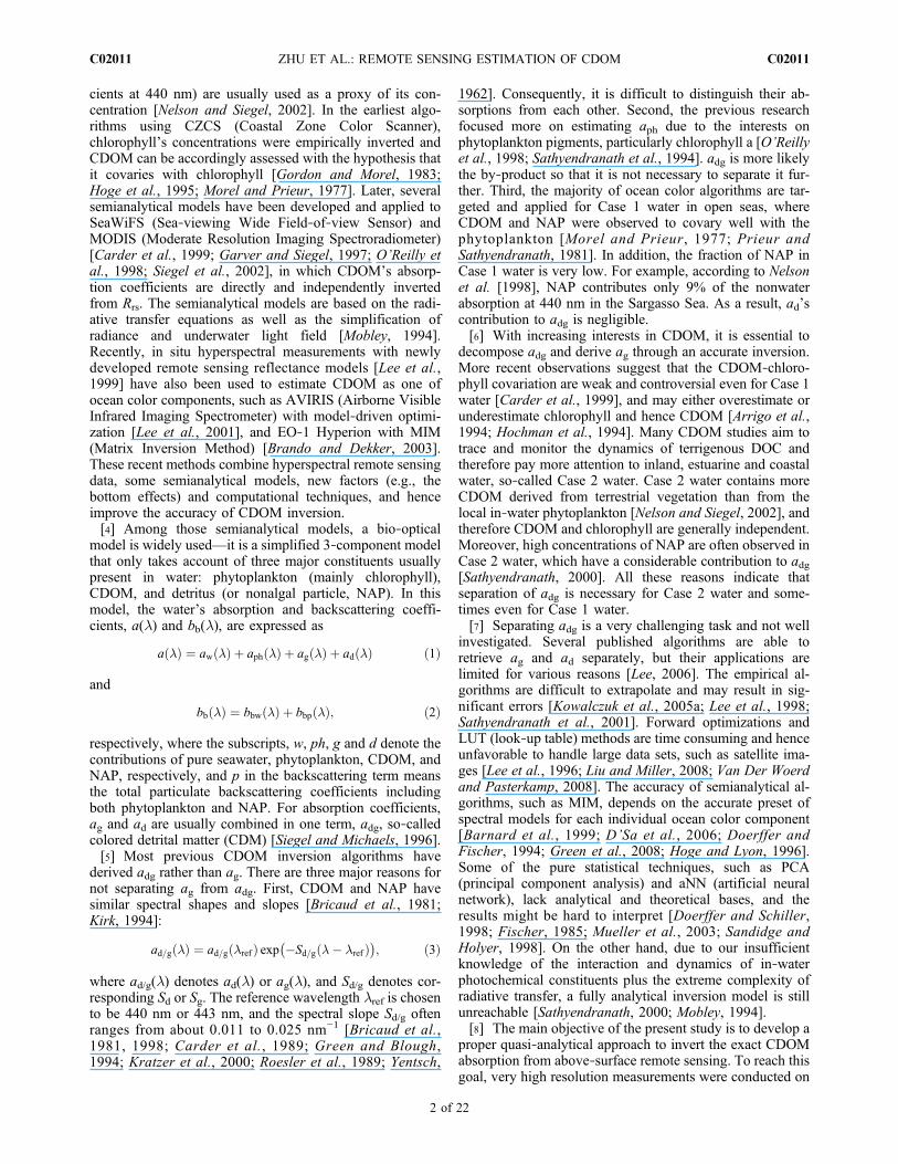
Estimation of chromophoric dissolved organic matterin the Mississippi and Atchafalaya river plume regionsusing above‐surface hyperspectral remote sensing

Weining Zhu,1 Qian Yu,1 Yong Q. Tian,2 Robert F. Chen,2 and G. Bernard Gardner2

Received 14 July 2010; revised 14 October 2010; accepted 29 November 2010; published 9 February 2011.

[1] A method for the inversion of hyperspectral remote sensing was developed todetermine the absorption coefficient for chromophoric dissolved organic matter (CDOM)in the Mississippi and Atchafalaya river plume regions and the northern Gulf of Mexico,where water types vary from Case 1 to turbid Case 2. Above‐surface hyperspectral remotesensing data were measured by a ship‐mounted spectroradiometer and then used toestimate CDOM. Simultaneously, water absorption and attenuation coefficients, CDOMand chlorophyll fluorescence, turbidities, and other related water properties were alsomeasured at very high resolution (0.5–2 m) using in situ, underwater, and flow‐through(shipboard, pumped) optical sensors. We separate ag, the absorption coefficient a ofCDOM, from adg (a of CDOM and nonalgal particles) based on two absorption‐backscattering relationships. The first is between ad (a of nonalgal particles) and bbp (totalparticulate backscattering coefficient), and the second is between ap (a of total particles)and bbp. These two relationships are referred as ad‐based and ap‐based methods,respectively. Consequently, based on Lee’s quasi‐analytical algorithm (QAA), wedeveloped the so‐called Extended Quasi‐Analytical Algorithm (QAA‐E) to decomposeadg, using both ad‐based and ap‐based methods. The absorption‐backscatteringrelationships and the QAA‐E were tested using synthetic and in situ data from theInternational Ocean‐Colour Coordinating Group (IOCCG) as well as our own field data.The results indicate the ad‐based method is relatively better than the ap‐based method.The accuracy of CDOM estimation is significantly improved by separating ag fromadg (R

2 = 0.81 and 0.65 for synthetic and in situ data, respectively). The sensitivities ofthe newly introduced coefficients were also analyzed to ensure QAA‐E is robust.

Citation: Zhu, W., Q. Yu, Y. Q. Tian, R. F. Chen, and G. B. Gardner (2011), Estimation of chromophoric dissolved organicmatter in the Mississippi and Atchafalaya river plume regions using above‐surface hyperspectral remote sensing, J. Geophys.Res., 116, C02011, doi:10.1029/2010JC006523.

1. Introduction

[2] Dissolved organic carbon (DOC), the carbon contentof dissolved organic matter (DOM), is one of the largestcarbon pools in aquatic systems [Amon and Benner, 1994;Carlson et al., 1994]. As the photoactive fraction of DOM,chromophoric dissolved organic matter (CDOM) in seawa-ter can be used as a tracer of terrestrial DOC in the marineenvironment [Blough et al., 1993; Del Castillo et al., 1999;Jerlov, 1976]. Many observations provide evidence of agood correlation between CDOM and DOC loading acrossthe different subcatchments [Ferrari et al., 1996; Kowalczuket al., 2005b; Mannino et al., 2008; Stedmon et al., 2006;Vodacek et al., 1997], despite the absence of this covariation

in a few cases [Chen et al., 2004]. Together with the othertwo ocean color components, chlorophyll and nonalgalparticles (NAP), CDOM plays an important role in deter-mining photochemical characteristics of water in nature; itshigh optical absorption at short wavelengths (350–440 nm)may affect the photosynthesis of aquatic phytoplankton[Bukata et al., 1995; Kirk, 1994]. In addition, due to itsbiotic sources, CDOM is also a good proxy for monitoringthe dynamics of organic ecosystems [Doney et al., 1995;Shooter and Brimblecombe, 1989; Valentine and Zepp,1993].[3] Since CDOM has an effect on the underwater light

field and water’s inherent optical properties (IOP), andconsequently determines the Lw (water‐leaving radiance) orRrs (remote sensing reflectance) received by above‐surfaceremote sensors, inversion of remote sensing data provides arapid and efficient approach to estimate CDOM within alarge spatial‐temporal scale [Sathyendranath, 2000; Lee,2006; Mobley, 1994]. Hence in ocean color sciences,CDOM’s absorption properties (e.g., its absorption coeffi-

1Department of Geosciences, University of Massachusetts Amherst,Amherst, Massachusetts, USA.

2Department of Environmental, Earth and Ocean Sciences, Universityof Massachusetts Boston, Boston, Massachusetts, USA.

Copyright 2011 by the American Geophysical Union.0148‐0227/11/2010JC006523

JOURNAL OF GEOPHYSICAL RESEARCH, VOL. 116, C02011, doi:10.1029/2010JC006523, 2011

C02011 1 of 22

cients at 440 nm) are usually used as a proxy of its con-centration [Nelson and Siegel, 2002]. In the earliest algo-rithms using CZCS (Coastal Zone Color Scanner),chlorophyll’s concentrations were empirically inverted andCDOM can be accordingly assessed with the hypothesis thatit covaries with chlorophyll [Gordon and Morel, 1983;Hoge et al., 1995; Morel and Prieur, 1977]. Later, severalsemianalytical models have been developed and applied toSeaWiFS (Sea‐viewing Wide Field‐of‐view Sensor) andMODIS (Moderate Resolution Imaging Spectroradiometer)[Carder et al., 1999; Garver and Siegel, 1997; O’Reilly etal., 1998; Siegel et al., 2002], in which CDOM’s absorp-tion coefficients are directly and independently invertedfrom Rrs. The semianalytical models are based on the radi-ative transfer equations as well as the simplification ofradiance and underwater light field [Mobley, 1994].Recently, in situ hyperspectral measurements with newlydeveloped remote sensing reflectance models [Lee et al.,1999] have also been used to estimate CDOM as one ofocean color components, such as AVIRIS (Airborne VisibleInfrared Imaging Spectrometer) with model‐driven optimi-zation [Lee et al., 2001], and EO‐1 Hyperion with MIM(Matrix Inversion Method) [Brando and Dekker, 2003].These recent methods combine hyperspectral remote sensingdata, some semianalytical models, new factors (e.g., thebottom effects) and computational techniques, and henceimprove the accuracy of CDOM inversion.[4] Among those semianalytical models, a bio‐optical

model is widely used—it is a simplified 3‐component modelthat only takes account of three major constituents usuallypresent in water: phytoplankton (mainly chlorophyll),CDOM, and detritus (or nonalgal particle, NAP). In thismodel, the water’s absorption and backscattering coeffi-cients, a(l) and bb(l), are expressed as

a �ð Þ ¼ aw �ð Þ þ aph �ð Þ þ ag �ð Þ þ ad �ð Þ ð1Þ

and

bb �ð Þ ¼ bbw �ð Þ þ bbp �ð Þ; ð2Þ

respectively, where the subscripts, w, ph, g and d denote thecontributions of pure seawater, phytoplankton, CDOM, andNAP, respectively, and p in the backscattering term meansthe total particulate backscattering coefficients includingboth phytoplankton and NAP. For absorption coefficients,ag and ad are usually combined in one term, adg, so‐calledcolored detrital matter (CDM) [Siegel and Michaels, 1996].[5] Most previous CDOM inversion algorithms have

derived adg rather than ag. There are three major reasons fornot separating ag from adg. First, CDOM and NAP havesimilar spectral shapes and slopes [Bricaud et al., 1981;Kirk, 1994]:

ad=g �ð Þ ¼ ad=g �refð Þ exp �Sd=g �� �refð Þ� �; ð3Þ

where ad/g(l) denotes ad(l) or ag(l), and Sd/g denotes cor-responding Sd or Sg. The reference wavelength lref is chosento be 440 nm or 443 nm, and the spectral slope Sd/g oftenranges from about 0.011 to 0.025 nm−1 [Bricaud et al.,1981, 1998; Carder et al., 1989; Green and Blough,1994; Kratzer et al., 2000; Roesler et al., 1989; Yentsch,

1962]. Consequently, it is difficult to distinguish their ab-sorptions from each other. Second, the previous researchfocused more on estimating aph due to the interests onphytoplankton pigments, particularly chlorophyll a [O’Reillyet al., 1998; Sathyendranath et al., 1994]. adg is more likelythe by‐product so that it is not necessary to separate it fur-ther. Third, the majority of ocean color algorithms are tar-geted and applied for Case 1 water in open seas, whereCDOM and NAP were observed to covary well with thephytoplankton [Morel and Prieur, 1977; Prieur andSathyendranath, 1981]. In addition, the fraction of NAP inCase 1 water is very low. For example, according to Nelsonet al. [1998], NAP contributes only 9% of the nonwaterabsorption at 440 nm in the Sargasso Sea. As a result, ad’scontribution to adg is negligible.[6] With increasing interests in CDOM, it is essential to

decompose adg and derive ag through an accurate inversion.More recent observations suggest that the CDOM‐chloro-phyll covariation are weak and controversial even for Case 1water [Carder et al., 1999], and may either overestimate orunderestimate chlorophyll and hence CDOM [Arrigo et al.,1994; Hochman et al., 1994]. Many CDOM studies aim totrace and monitor the dynamics of terrigenous DOC andtherefore pay more attention to inland, estuarine and coastalwater, so‐called Case 2 water. Case 2 water contains moreCDOM derived from terrestrial vegetation than from thelocal in‐water phytoplankton [Nelson and Siegel, 2002], andtherefore CDOM and chlorophyll are generally independent.Moreover, high concentrations of NAP are often observed inCase 2 water, which have a considerable contribution to adg[Sathyendranath, 2000]. All these reasons indicate thatseparation of adg is necessary for Case 2 water and some-times even for Case 1 water.[7] Separating adg is a very challenging task and not well

investigated. Several published algorithms are able toretrieve ag and ad separately, but their applications arelimited for various reasons [Lee, 2006]. The empirical al-gorithms are difficult to extrapolate and may result in sig-nificant errors [Kowalczuk et al., 2005a; Lee et al., 1998;Sathyendranath et al., 2001]. Forward optimizations andLUT (look‐up table) methods are time consuming and henceunfavorable to handle large data sets, such as satellite ima-ges [Lee et al., 1996; Liu and Miller, 2008; Van Der Woerdand Pasterkamp, 2008]. The accuracy of semianalytical al-gorithms, such as MIM, depends on the accurate preset ofspectral models for each individual ocean color component[Barnard et al., 1999; D’Sa et al., 2006; Doerffer andFischer, 1994; Green et al., 2008; Hoge and Lyon, 1996].Some of the pure statistical techniques, such as PCA(principal component analysis) and aNN (artificial neuralnetwork), lack analytical and theoretical bases, and theresults might be hard to interpret [Doerffer and Schiller,1998; Fischer, 1985; Mueller et al., 2003; Sandidge andHolyer, 1998]. On the other hand, due to our insufficientknowledge of the interaction and dynamics of in‐waterphotochemical constituents plus the extreme complexity ofradiative transfer, a fully analytical inversion model is stillunreachable [Sathyendranath, 2000; Mobley, 1994].[8] The main objective of the present study is to develop a

proper quasi‐analytical approach to invert the exact CDOMabsorption from above‐surface remote sensing. To reach thisgoal, very high resolution measurements were conducted on

ZHU ET AL.: REMOTE SENSING ESTIMATION OF CDOM C02011C02011

2 of 22

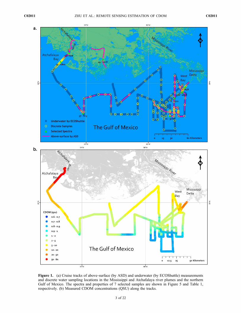
Figure 1. (a) Cruise tracks of above‐surface (by ASD) and underwater (by ECOShuttle) measurementsand discrete water sampling locations in the Mississippi and Atchafalaya river plumes and the northernGulf of Mexico. The spectra and properties of 7 selected samples are shown in Figure 5 and Table 1,respectively. (b) Measured CDOM concentrations (QSU) along the tracks.

ZHU ET AL.: REMOTE SENSING ESTIMATION OF CDOM C02011C02011

3 of 22

the Mississippi and Atchafalaya river plumes as well as thenorthern Gulf of Mexico, where CDOM, chlorophyll andNAP’s variations are large and water types are diverse fromsimple Case 1 to complex Case 2. About 300,000 in situmeasurements of CDOM, chlorophyll, NAP, water’s IOPsand other properties, as well as 20,000 water hyperspectrawere collected almost simultaneously, providing a huge dataset for ocean color study. Based on the former quasi‐ana-lytical algorithm (QAA), we developed an extension toseparate ag from adg. The results show that the proposedseparation method performs excellently and is promising forfuture satellite image inversion.

2. Data Acquisition

2.1. Study Site

[9] The Mississippi River is the longest river in the UnitedStates, and its watershed occupies about 41% of total con-tinental area of the Unite States. At Old River Junction, aman‐made system controls the flow of the Mississippi Riverto the Gulf of Mexico. The U.S. Army Corps of Engineersreports that seventy percent of the flow drains out of theBirdfoot region through the lower Mississippi River whilethirty percent is diverted to the Atchafalaya basin, formingthe Atchafalaya River [U.S. Army Corps of Engineers,2008]. Both outlets in the Gulf of Mexico form largeplumes containing high sediment and organic matter con-centrations. The lower Atchafalaya River passes throughwetlands, salt marshes and bayous, and empties into theshallow Atchafalaya Bay with a large capacity to trap sed-iment. Also, the near coastal wetlands are highly productiveecosystems which interact with riverine and estuarine watersand represent a source of coastal CDOM [Lane et al., 2002;Pakulski et al., 2000]. On the other hand, the lower Mis-sissippi holds a catchment with low vegetation coverage thathas been highly channelized. Therefore, the interaction ofthe river with historical floodplains is greatly reduced and istherefore expected to have lower CDOM inputs to the Gulfof Mexico than the Atchafalaya.[10] The in situ CDOM concentration and spectral data

were measured on the RV Pelican during a 7 day cruise, 23–29 August 2007, in the Mississippi and Atchafalaya riverplume regions as well as the northern Gulf of Mexico. Thecruise tracks were designed to cross the CDOM gradients inthe plumes, aiming to capture the largest variations inCDOM. The data acquisition activities include (1) contin-uous above‐surface hyperspectral measurements of waterapparent optical properties (AOP), (2) continuous under-water measurements of temperature, salinity, density, dis-solved oxygen and UV radiance, CDOM fluorescence,chlorophyll fluorescence, optical backscatter, and depth, (3)continuous measurements of the IOPs (absorption andbackscattering coefficients) of water pumped from thesampling platform, and (4) discrete water sampling from thepumped water for analysis of absorption spectra, CDOMfluorescence, and dissolved organic carbon in the labora-tory. The GPS‐derived ship position was recorded concur-rently with the in situ data. The site map, cruise track, andsampling locations of above measurements are illustrated inFigure 1a.

2.2. Above‐Surface Hyperspectral Measurements

[11] The above‐surface remote sensing reflectance ofseawater was measured by a portable spectroradiometer(Applied Spectral Devices FieldSpec®3), with a full spectralrange (350–2500 nm). The spectral sampling interval ofoutput is 1 nm. The fiber optic collection sensor wasmounted on the bow of the vessel pointed straight down atthe sea surface at a height of approximately 4 m. The sensorwas mounted in a way that the sensor could be turned byhand to measure water total radiance/reflectance (down), skyradiance (up), or at a white barium oxide white board(down) for calibration. The above‐surface measurement wasreferred to NASA’s ocean optics protocols for satelliteocean color sensor validation [Mueller et al., 2003].[12] The measurements were continuous during the day-

time, from around 08:30 to 18:30 local time. Data were notcollected during very high seas that created white caps.During the entire cruise, we collected 75 data sets withapproximately 20,000 hyperspectral samples. Each data setcontains 100 to 3000 samples that were obtained undersimilar illumination conditions with individual sky radiancemeasurements and white board calibrations. The calibrationfrequency between each data set depended on the change ofsolar zenith and illumination conditions throughout the day,particularly considering cloud and wind conditions, typi-cally every 20–30 min or less. The frequency of samplingwas approximately 5–20 s per sample depending on CDOMgradient and navigation speed (lower frequency for open seaand higher frequency for river plume regions). Each sampleis an average of 10 spectral measures to reduce the noise[Analytical Spectral Devices, Inc., 2009]. The weatherduring the cruise was in general sunny, occasionally withlight clouds and gentle wind, except for a few hours ofstrong winds on 23 August. Sampling locations were re-corded by a GPS unit synchronized with the AnalyticalSpectral Devices (ASD) spectroradiometer.[13] Compared with the satellite images, the in situ above‐

surface hyperspectral measurements bear two advantages:(1) much less atmospheric effect and (2) better synchroni-zation to the in situ CDOM measurements. One goal of ourproject is to investigate whether above‐surface hyperspectralremote sensing is capable of estimating CDOM concentra-tion in ocean and coastal waters with satisfactory accuracy.This knowledge will contribute to our ability to estimatecoastal CDOM concentrations from hyperspectral satelliteimages such as those from EO‐1 Hyperion.

2.3. Underwater Measurements

[14] In situ underwater measurements were carried outusing the ECOShuttle, a towed, undulating vehicle based onthe Nu‐Shuttle manufactured by Chelsea Instruments.Instrumentation mounted inside the ECOShuttle include aSeaBird Electronics SBE 9/11 CTD system providing tem-perature, salinity and depth measurements; a CDOM fluo-rometer, a chlorophyll fluorometer and an opticalbackscatter sensor (OBS) manufactured by Seapoint Sen-sors, Inc; and a YSI dissolved oxygen sensor provided bySeaBird Electronics. The CTD is calibrated at the factoryannually. CDOM voltages were compared with discretesamples and converted to quinine sulfate units (QSU)equivalent to 1mg/l of quinine sulfate at pH = 2, lex = 337 nm,

ZHU ET AL.: REMOTE SENSING ESTIMATION OF CDOM C02011C02011

4 of 22

and lem = 450 nm. Chlorophyll fluorescence was calibratedusing the factory suggested conversion factor. The ECOSh-uttle was generally programmed for a sawtooth pattern from2–3 m depth (just below the influence of the ship’s wake) to adepth 5 m above the bottom (to avoid the bottom). Ship speedwas 6–8 knots. The sampling resolution was in the range of0.5–2m (around 3 samples per second) along the cruise track.About 1,000,000 underwater measurements were acquired.To minimize the random error, we averaged the successivemeasurements within every 0.2 m depth, which resulted in300,000 measurements used in the study.[15] In addition, a stainless steel well pump mounted on

the underside of the ECOShuttle pumped uncontaminated(only touches stainless steel and Teflon) seawater into theshipboard lab via a 0.5‐inch ID Teflon tube in the tow cable.This seawater flow was distributed into a Wetlabs AC‐9multispectral absorption meter that measures the water’stotal attenuation and absorption coefficients at 9 wave-lengths (412, 440, 488, 510, 532, 555, 650, 676, 715 nm).Milli‐Q water was used as a reference. In addition, theflowing seawater supplies a source for discrete sampleanalysis of DOC and optical properties. Complete details ofthe ECOShuttle system are given by Chen [1999], Chen etal. [2004], and Chen and Gardner [2004].

2.4. Discrete Samples

[16] Discrete water samples supplied by the ECOShuttle’spumping system were collected to calibrate the real timeunderway measurements (Figure 1a). The interval of sam-pling was generally determined by the ECOShuttle depth,the sampling lag time and the location. When a sample wasto be taken, an instantaneous record of the in situ data wasproduced and a stopwatch started to determine the exacttime for collection. Samples were drawn precisely after thedetermined delay time had passed (the ECOShuttle gener-ally spent 10–20 s at the surface). The delay time wasdetermined by matching salinity minima and maxima as theECOShuttle undulated through a river plume, usuallyaround 4 min. Careful alignment of in‐line data withECOShuttle data was made after the cruise. Fluorescence offiltered seawater samples was measured with a PhotonTechnologies International Quantum Master‐1 spectrofluo-rometer equipped with a double excitation monochromator,a single emission monochromator and a cooled photo-multiplier assembly. CDOM absorption spectra (200–800nm) were measured by a Cary 50 spectrophotometer with a1 cm path length cell. The details of lab processing andcomputation were described by Huang and Chen [2009].

3. Methods

3.1. Data Preprocessing

3.1.1. Above‐Surface Hyperspectra[17] The radiance received by the above‐surface spectro-

radiometer includes both water‐leaving radiance and theradiance from the water surface reflection. Water surfacereflection contains no information about the in‐water con-stituents, but contaminates the subsurface volumetric radi-ance. Before inversion, the surface radiance need to beremoved to obtain the remote sensing reflectance or water‐leaving radiance, which are the eligible inputs of inversealgorithms [Yu et al., 2010].

[18] Remote sensing reflectanceRrs at given direction (�,’)and wavelength l is calculated by Mobley [1999]

Rrs ¼ Rg Lt � Lrð Þ�Lg

; ð4Þ

where Lt is the total water radiance received by sensors, and Lris the radiance reflected by the sea surface. Hence Lt − Lr isthe water‐leaving radiance; Lg is the radiance reflected by theSpectralon reference panel (white reference); and the Rg is thereflectance of the white reference. Since the white reference isa Lambertian surface, Rg is equivalent to irradiance reflec-tance, defined as the ratio of upward planar irradiance anddownward planar irradiance. pLg/Rg gives the downwellingspectral plane irradiance incident onto the sea surface.[19] In equation (4), technically we could not measure Lr

directly but it can be approximately computed by Lr ≈ rLs,where Ls is sky radiance from the corresponding incidentangle and the r is the ratio representing the proportion of Lrto Ls. In our cruise, we mainly recorded the total waterreflectance Rt, instead of the Lt (only a small number of Ltwere recorded for calibration purpose). In ASD, Rt isdetermined by Rt = Lt/Lg. Therefore equation (4) could berewritten by all directly measured variables, except r, that is,

Rrs ¼ Rg

�Rt � �Ls

Lg

� �: ð5Þ

Rg is in the range of 0.990 to 0.992 at wavelengths from 400to 700 nm. r was simulated individually for each data setusing Hydro‐Ecolight® [Mobley and Sundman, 2008], withspecific in situ solar zenith, wind speed, cloud cover, andother atmospheric properties. We used a nadir view, ratherthan the recommended viewing angles of zenith 45° andazimuth 135°. The reason is for a consecutive measurementalong the cruise, this nadir viewing angle keeps fixed sen-sor‐Sun geometry, and the sensor azimuth angle ’ is inde-pendent of ship moving direction. Therefore the sensor viewangle is consistent while the vessel frequently alters itsnavigating direction at varying time of day (different solarangle). In addition, according to the previous results[Mobley, 1999, Figure 7], the nadir view, that is, � = 0° and’ = 0°, is beneficial in removing water surface reflectance.In our calculation, we found that r slightly varied with solarzenith and wind speed, but was highly impacted by cloudcover. For solar zenith � > 30°, wind speed < 5 m/s and clearsky, r for the nadir viewing is approximately 0.021. Thespectral data measured with solar zenith � < 20° (around11:30 A.M.–12:30 P.M.), wind speed > 10 m/s, or undercloud shadow were not included in the analysis due to theinduced high uncertainty.3.1.2. CDOM Concentration and Water’s IOP[20] Due to complex and variable CDOM chemistry,

CDOM concentration is usually represented by its opticalproperties, for example, the fluorescence intensity, ratherthan its physical mass, as the mg/l or g/l used for chlorophylland NAP. In ocean color science, CDOM’s absorptioncoefficient at 440 nm, ag(440), is often taken as the proxy ofits concentration and remote sensing inversion also oftenreturns ag(440) [Lee, 2006]. In our underwater continuousmeasurement, CDOM concentrations were measured by afluorometer that returns voltages (V) as CDOM’s proxy. In

ZHU ET AL.: REMOTE SENSING ESTIMATION OF CDOM C02011C02011

5 of 22

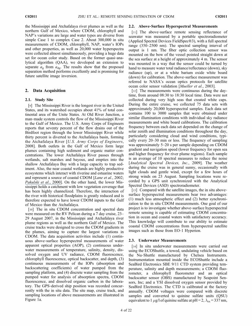
our discrete samples, we measured CDOM fluorescence inQSU and CDOM absorption (ag). Those three CDOMproxies, QSU, ag(440) and instantaneous voltage, have beenfound strongly correlated (Figure 2). Based on these linearrelationships, the voltages continuously measured can beconverted to QSU or ag.[21] We used an empirical approach to compute in situ

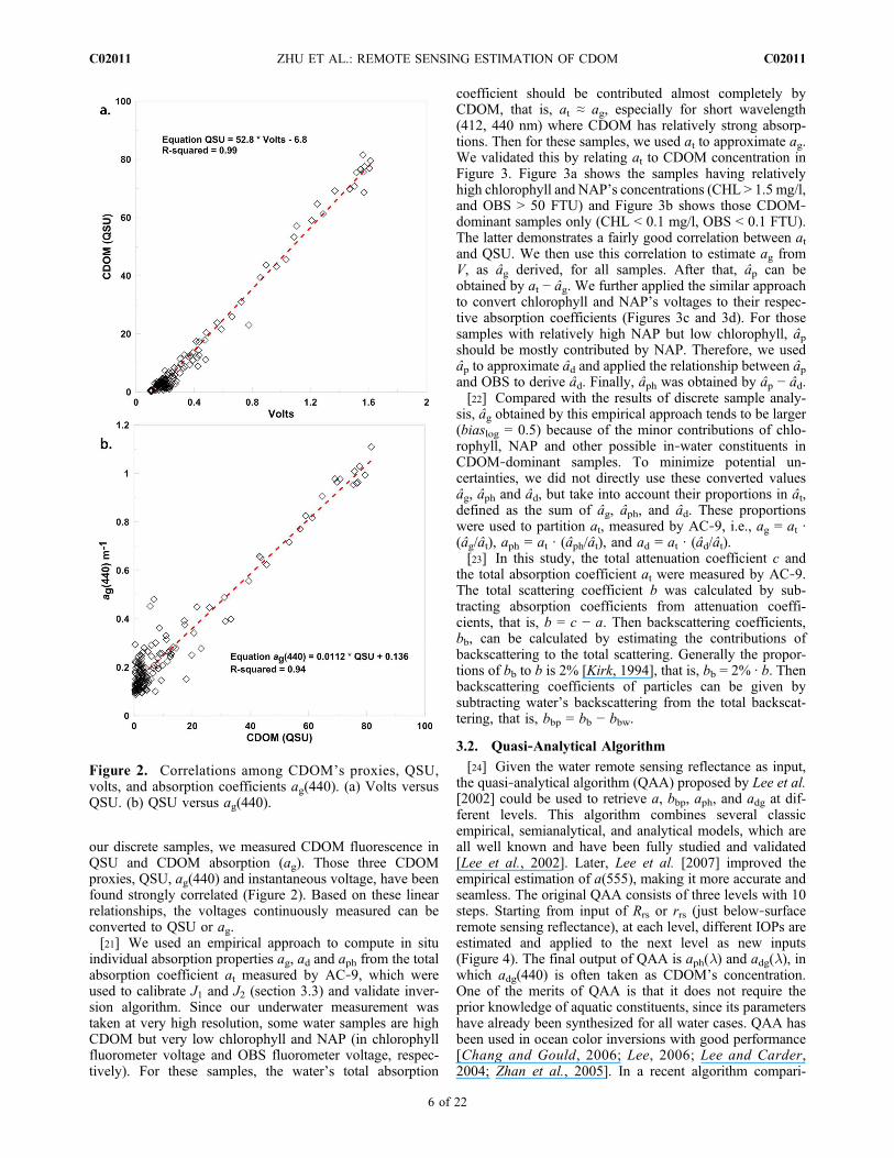
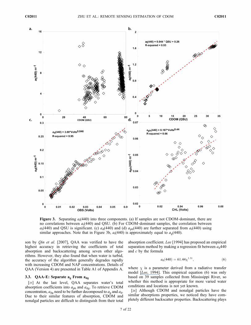
individual absorption properties ag, ad and aph from the totalabsorption coefficient at measured by AC‐9, which wereused to calibrate J1 and J2 (section 3.3) and validate inver-sion algorithm. Since our underwater measurement wastaken at very high resolution, some water samples are highCDOM but very low chlorophyll and NAP (in chlorophyllfluorometer voltage and OBS fluorometer voltage, respec-tively). For these samples, the water’s total absorption

coefficient should be contributed almost completely byCDOM, that is, at ≈ ag, especially for short wavelength(412, 440 nm) where CDOM has relatively strong absorp-tions. Then for these samples, we used at to approximate ag.We validated this by relating at to CDOM concentration inFigure 3. Figure 3a shows the samples having relativelyhigh chlorophyll and NAP’s concentrations (CHL > 1.5 mg/l,and OBS > 50 FTU) and Figure 3b shows those CDOM‐dominant samples only (CHL < 0.1 mg/l, OBS < 0.1 FTU).The latter demonstrates a fairly good correlation between atand QSU. We then use this correlation to estimate ag fromV, as âg derived, for all samples. After that, âp can beobtained by at − âg. We further applied the similar approachto convert chlorophyll and NAP’s voltages to their respec-tive absorption coefficients (Figures 3c and 3d). For thosesamples with relatively high NAP but low chlorophyll, âpshould be mostly contributed by NAP. Therefore, we usedâp to approximate âd and applied the relationship between âpand OBS to derive âd. Finally, âph was obtained by âp − âd.[22] Compared with the results of discrete sample analy-

sis, âg obtained by this empirical approach tends to be larger(biaslog = 0.5) because of the minor contributions of chlo-rophyll, NAP and other possible in‐water constituents inCDOM‐dominant samples. To minimize potential un-certainties, we did not directly use these converted valuesâg, âph and âd, but take into account their proportions in ât,defined as the sum of âg, âph, and âd. These proportionswere used to partition at, measured by AC‐9, i.e., ag = at ·(âg/ât), aph = at · (âph/ât), and ad = at · (âd/ât).[23] In this study, the total attenuation coefficient c and

the total absorption coefficient at were measured by AC‐9.The total scattering coefficient b was calculated by sub-tracting absorption coefficients from attenuation coeffi-cients, that is, b = c − a. Then backscattering coefficients,bb, can be calculated by estimating the contributions ofbackscattering to the total scattering. Generally the propor-tions of bb to b is 2% [Kirk, 1994], that is, bb = 2% · b. Thenbackscattering coefficients of particles can be given bysubtracting water’s backscattering from the total backscat-tering, that is, bbp = bb − bbw.

3.2. Quasi‐Analytical Algorithm

[24] Given the water remote sensing reflectance as input,the quasi‐analytical algorithm (QAA) proposed by Lee et al.[2002] could be used to retrieve a, bbp, aph, and adg at dif-ferent levels. This algorithm combines several classicempirical, semianalytical, and analytical models, which areall well known and have been fully studied and validated[Lee et al., 2002]. Later, Lee et al. [2007] improved theempirical estimation of a(555), making it more accurate andseamless. The original QAA consists of three levels with 10steps. Starting from input of Rrs or rrs (just below‐surfaceremote sensing reflectance), at each level, different IOPs areestimated and applied to the next level as new inputs(Figure 4). The final output of QAA is aph(l) and adg(l), inwhich adg(440) is often taken as CDOM’s concentration.One of the merits of QAA is that it does not require theprior knowledge of aquatic constituents, since its parametershave already been synthesized for all water cases. QAA hasbeen used in ocean color inversions with good performance[Chang and Gould, 2006; Lee, 2006; Lee and Carder,2004; Zhan et al., 2005]. In a recent algorithm compari-

Figure 2. Correlations among CDOM’s proxies, QSU,volts, and absorption coefficients ag(440). (a) Volts versusQSU. (b) QSU versus ag(440).

ZHU ET AL.: REMOTE SENSING ESTIMATION OF CDOM C02011C02011

6 of 22

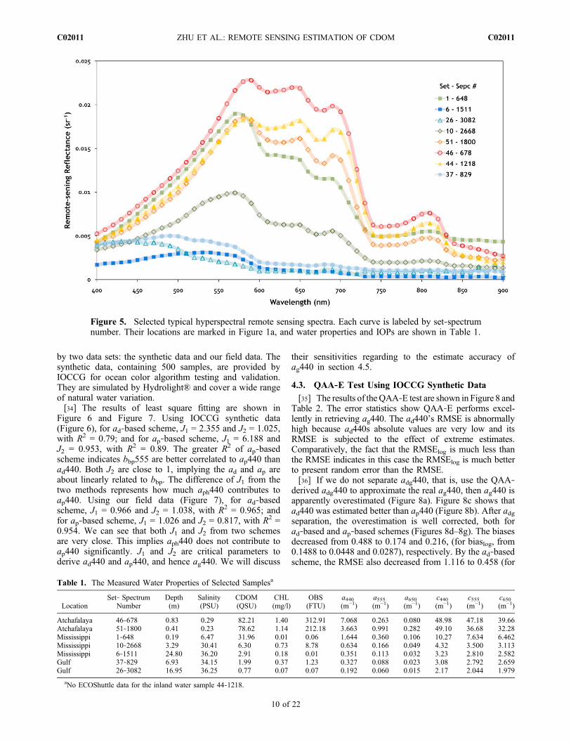
son by Qin et al. [2007], QAA was verified to have thehighest accuracy in retrieving the coefficients of totalabsorption and backscattering among seven other algo-rithms. However, they also found that when water is turbid,the accuracy of the algorithm generally degrades rapidlywith increasing CDOM and NAP concentrations. Details ofQAA (Version 4) are presented in Table A1 of Appendix A.

3.3. QAA‐E: Separate ag From adg[25] At the last level, QAA separates water’s total

absorption coefficients into aph and adg. To retrieve CDOMconcentration, adg need to be further decomposed to ag and ad.Due to their similar features of absorption, CDOM andnonalgal particles are difficult to distinguish from their total

absorption coefficient. Lee [1994] has proposed an empiricalseparation method by making a regression fit between ad440and c by the formula

ad 440ð Þ ¼ 61:44�1:31; ð6Þ

where c is a parameter derived from a radiative transfermodel [Lee, 1994]. This empirical equation (6) was onlybased on 39 samples collected from Mississippi River, sowhether this method is appropriate for more varied waterconditions and locations is not yet known.[26] Although CDOM and nonalgal particles have the

similar absorptions properties, we noticed they have com-pletely different backscatter properties. Backscattering plays

Figure 3. Separating at(440) into three components. (a) If samples are not CDOM‐dominant, there areno correlations between at(440) and QSU. (b) For CDOM‐dominant samples, the correlation betweenat(440) and QSU is significant. (c) ad(440) and (d) aph(440) are further separated from at(440) usingsimilar approaches. Note that in Figure 3b, at(440) is approximately equal to ag(440).

ZHU ET AL.: REMOTE SENSING ESTIMATION OF CDOM C02011C02011

7 of 22

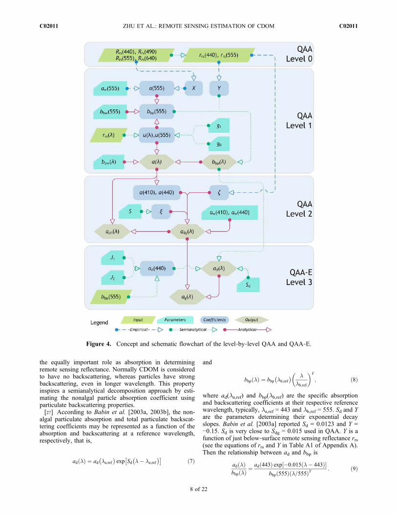
the equally important role as absorption in determiningremote sensing reflectance. Normally CDOM is consideredto have no backscattering, whereas particles have strongbackscattering, even in longer wavelength. This propertyinspires a semianalytical decomposition approach by esti-mating the nonalgal particle absorption coefficient usingparticulate backscattering properties.[27] According to Babin et al. [2003a, 2003b], the non-

algal particulate absorption and total particulate backscat-tering coefficients may be represented as a function of theabsorption and backscattering at a reference wavelength,respectively, that is,

ad �ð Þ ¼ ad �a;ref

� �exp Sd �� �a;ref

� �� � ð7Þ

and

bbp �ð Þ ¼ bbp �b;ref

� � �

�b;ref

� �Y

; ð8Þ

where ad(la,ref) and bbp(lb,ref) are the specific absorptionand backscattering coefficients at their respective referencewavelength, typically, la,ref = 443 and lb,ref = 555. Sd and Yare the parameters determining their exponential decayslopes. Babin et al. [2003a] reported Sd = 0.0123 and Y =−0.15. Sd is very close to Sdg = 0.015 used in QAA. Y is afunction of just below‐surface remote sensing reflectance rrs(see the equations of rrs and Y in Table A1 of Appendix A).Then the relationship between ad and bbp is

ad �ð Þbbpð�Þ ¼

ad 443ð Þ exp½�0:015 �� 443ð Þ�bbp 555ð Þ �=555ð ÞY : ð9Þ

Figure 4. Concept and schematic flowchart of the level‐by‐level QAA and QAA‐E.

ZHU ET AL.: REMOTE SENSING ESTIMATION OF CDOM C02011C02011

8 of 22

ad(l) could be derived through equation (9) as long as thebbp(l) and the ratio q = ad443/bbp555 are known. In QAA,bbp(l) is already retrieved, so we only need to determine q.ad443 and bbp555 are both connected to suspended par-ticulate matter (SPM); their ratio could be derived fromtwo equations suggested by Babin et al. [2003a, 2003b]:

ad 443ð Þ : SPM ¼ 0:041

bbp 555ð Þ : SPM ¼ 0:51

Therefore, we get q = 0.0804, namely, ad443 = 0.0804bbp555.However, for ocean color components, the relationshipbetween their optical properties and physical concentrations isoften expressed by a power function. For instance, the specificabsorption coefficients of chlorophyll aph*(440) = 0.06[C]0.65

[Maritorena et al., 2000]. In addition, equation (6) impliesad440 is a power function of a radiative transfer parameter.Based on the above consideration, if ad443 and bbp555 areboth power functions of SPM, then q is also a power functionof SPM. This equally means ad443 could be expressed as apower function of bbp555, that is,

ad 440ð Þ ¼ J1bbp 555ð ÞJ2 : ð10Þ

Then coefficients J1 and J2 can be estimated from a least squarefit. Once ad443 is known (here assuming it is equal to ad440),we then obtain ag440 by subtracting ad443 from the knownadg440. The full flowchart and equations of QAA‐E are alsosummarized in Figure 4 and Table A2 of Appendix A,respectively.[28] However, according to Babin et al. [2003b], the

relationship between ad440 and SPM may not be accuratebecause the phytoplankton is a fraction of the SPM, whichdoes not contribute to ad440 but does to aph440. Therefore,the exact relationship should be created between the ap440(the sum of ad440 and aph440) and SPM. In the same way,we can further obtain the following expression:

ap 440ð Þ ¼ J1bbp 555ð ÞJ2 : ð11Þ

Then an alternative method to retrieve ag440 is using

ag 440ð Þ ¼ at 440ð Þ � ap 440ð Þ; ð12Þ

where at440 is the total absorption coefficient for the threeocean color components. It is derived by QAA at the level 1.[29] In this study, the above two schemes, called ad‐based

and ap‐based, respectively, were both applied to retrieveag440. If adg is directly used to represent ag440 withoutdecomposition, we call it an adg‐based scheme. The resultsof J1 and J2 and comparison of the three schemes are shownin section 3.4.

3.4. Accuracy Assessment

[30] Algorithm performance was evaluated using thefollowing three statistics: the relative error, normalizedbias, and root mean square error (RMSE). The former two

assess systematic error, and the latter assesses randomerror:

Errori ¼ xmodeli �xobsi

xobsi

bias ¼ Mean Errorð Þ

RMSE ¼ Stdev Errorð Þ;

where xmodel is the variable of interest derived from proposedmodels or algorithms, xobs is the same variable known as thetruth, either observed from in situ measurement or the syn-thetic simulation, and “Mean” and “Stdev” are the mean andstandard deviation of errors, respectively.[31] The statistical distributions of ocean color compo-

nents often follow lognormal distribution [O’Reilly et al.,1998]. Therefore, the error, bias and RMSE can be alsonormalized as

Errorlog i ¼ log xmodeli

� �� log xobsi

� �

biaslog ¼ Mean Errorlog� �

RMSElog ¼ 1n�2

Pni¼1

log xmodeli

� �� log xobsi

� �� �2� �12

;

where n is the number of observations [Lee, 2006].

4. Results and Discussion

4.1. The Field‐Measured CDOM and Water’s IOPsand AOPs

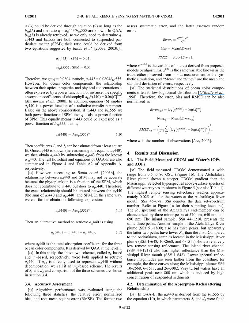
[32] The field‐measured CDOM demonstrated a widerange from 0.6 to 80 QSU (Figure 1b). The AtchafalayaRiver plume shows a steeper CDOM gradient than theMississippi. Selected hyperspectral above‐surface spectra ofdifferent water types are shown in Figure 5 (see also Table 1).The highest remote sensing reflectance reaches approxi-mately 0.025 sr−1 for the waters at the Atchafalaya Rivermouth (SS# 46‐678; SS# denotes the data set‐spectrumnumber. Refer to Figure 1a for their sampling locations).The Rrs spectrum of the Atchafalaya end‐member can becharacterized by three minor peaks at 570 nm, 640 nm, and690 nm. The inland sample, SS# 44‐1218, presents thesame three peaks. Another sample in the Atchafalaya Riverplume (SS# 51‐1800) also has three peaks, but apparentlythe latter two peaks have lower Rrs than the first. Comparedto the Atchafalaya, samples located in the Mississippi Riverplume (SS# 1‐648, 10‐2668, and 6‐1511) show a relativelylow remote sensing reflectance. The inland river channel(SS# 44‐1218) also has higher reflectance than the Mis-sissippi River mouth (SS# 1‐648). Lower spectral reflec-tance magnitudes are seen farther from the coastline, forexample, the three curves along the Mississippi plume: SS#10‐2668, 6‐1511, and 26‐3082. Very turbid waters have anadditional peak near 800 nm which is induced by highconcentration of suspended sediments.

4.2. Determination of the Absorption‐BackscatteringRelationship

[33] In QAA‐E, the ad440 is derived from the bbp555 bythe equation (10), in which parameters J1 and J2 were fitted

ZHU ET AL.: REMOTE SENSING ESTIMATION OF CDOM C02011C02011

9 of 22

by two data sets: the synthetic data and our field data. Thesynthetic data, containing 500 samples, are provided byIOCCG for ocean color algorithm testing and validation.They are simulated by Hydrolight® and cover a wide rangeof natural water variation.[34] The results of least square fitting are shown in

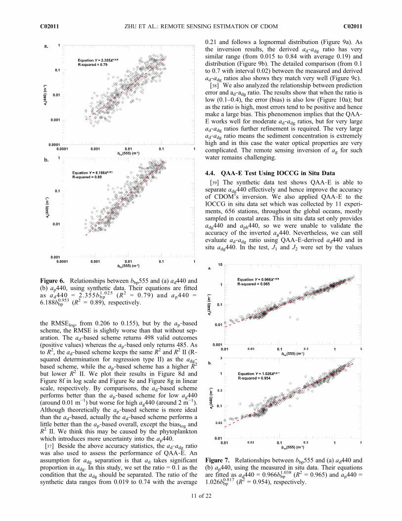
Figure 6 and Figure 7. Using IOCCG synthetic data(Figure 6), for ad‐based scheme, J1 = 2.355 and J2 = 1.025,with R2 = 0.79; and for ap‐based scheme, J1 = 6.188 andJ2 = 0.953, with R2 = 0.89. The greater R2 of ap‐basedscheme indicates bbp555 are better correlated to ap440 thanad440. Both J2 are close to 1, implying the ad and ap areabout linearly related to bbp. The difference of J1 from thetwo methods represents how much aph440 contributes toap440. Using our field data (Figure 7), for ad‐basedscheme, J1 = 0.966 and J2 = 1.038, with R2 = 0.965; andfor ap‐based scheme, J1 = 1.026 and J2 = 0.817, with R2 =0.954. We can see that both J1 and J2 from two schemesare very close. This implies aph440 does not contribute toap440 significantly. J1 and J2 are critical parameters toderive ad440 and ap440, and hence ag440. We will discuss

their sensitivities regarding to the estimate accuracy ofag440 in section 4.5.

4.3. QAA‐E Test Using IOCCG Synthetic Data

[35] The results of the QAA‐E test are shown in Figure 8 andTable 2. The error statistics show QAA‐E performs excel-lently in retrieving ag440. The ad440’s RMSE is abnormallyhigh because ad440s absolute values are very low and itsRMSE is subjected to the effect of extreme estimates.Comparatively, the fact that the RMSElog is much less thanthe RMSE indicates in this case the RMSElog is much betterto present random error than the RMSE.[36] If we do not separate adg440, that is, use the QAA‐

derived adg440 to approximate the real ag440, then ag440 isapparently overestimated (Figure 8a). Figure 8c shows thatad440 was estimated better than ap440 (Figure 8b). After adgseparation, the overestimation is well corrected, both forad‐based and ap‐based schemes (Figures 8d–8g). The biasesdecreased from 0.488 to 0.174 and 0.216, (for biaslog, from0.1488 to 0.0448 and 0.0287), respectively. By the ad‐basedscheme, the RMSE also decreased from 1.116 to 0.458 (for

Figure 5. Selected typical hyperspectral remote sensing spectra. Each curve is labeled by set‐spectrumnumber. Their locations are marked in Figure 1a, and water properties and IOPs are shown in Table 1.

Table 1. The Measured Water Properties of Selected Samplesa

LocationSet‐ Spectrum

NumberDepth(m)

Salinity(PSU)

CDOM(QSU)

CHL(mg/l)

OBS(FTU)

a440(m−1)

a555(m−1)

a650(m−1)

c440(m−1)

c555(m−1)

c650(m−1)

Atchafalaya 46‐678 0.83 0.29 82.21 1.40 312.91 7.068 0.263 0.080 48.98 47.18 39.66Atchafalaya 51‐1800 0.41 0.23 78.62 1.14 212.18 3.663 0.991 0.282 49.10 36.68 32.28Mississippi 1‐648 0.19 6.47 31.96 0.01 0.06 1.644 0.360 0.106 10.27 7.634 6.462Mississippi 10‐2668 3.29 30.41 6.30 0.73 8.78 0.634 0.166 0.049 4.32 3.500 3.113Mississippi 6‐1511 24.80 36.20 2.91 0.18 0.01 0.351 0.113 0.032 3.23 2.810 2.582Gulf 37‐829 6.93 34.15 1.99 0.37 1.23 0.327 0.088 0.023 3.08 2.792 2.659Gulf 26‐3082 16.95 36.25 0.77 0.07 0.07 0.192 0.060 0.015 2.17 2.044 1.979

aNo ECOShuttle data for the inland water sample 44‐1218.

ZHU ET AL.: REMOTE SENSING ESTIMATION OF CDOM C02011C02011

10 of 22

the RMSElog, from 0.206 to 0.155), but by the ap‐basedscheme, the RMSE is slightly worse than that without sep-aration. The ad‐based scheme returns 498 valid outcomes(positive values) whereas the ap‐based only returns 485. Asto R2, the ad‐based scheme keeps the same R2 and R2 II (R‐squared determination for regression type II) as the adg‐based scheme, while the ap‐based scheme has a higher R2

but lower R2 II. We plot their results in Figure 8d andFigure 8f in log scale and Figure 8e and Figure 8g in linearscale, respectively. By comparisons, the ad‐based schemeperforms better than the ap‐based scheme for low ag440(around 0.01 m−1) but worse for high ag440 (around 2 m−1).Although theoretically the ap‐based scheme is more idealthan the ad‐based, actually the ad‐based scheme performs alittle better than the ap‐based overall, except the biaslog andR2 II. We think this may be caused by the phytoplanktonwhich introduces more uncertainty into the ap440.[37] Beside the above accuracy statistics, the ad‐adg ratio

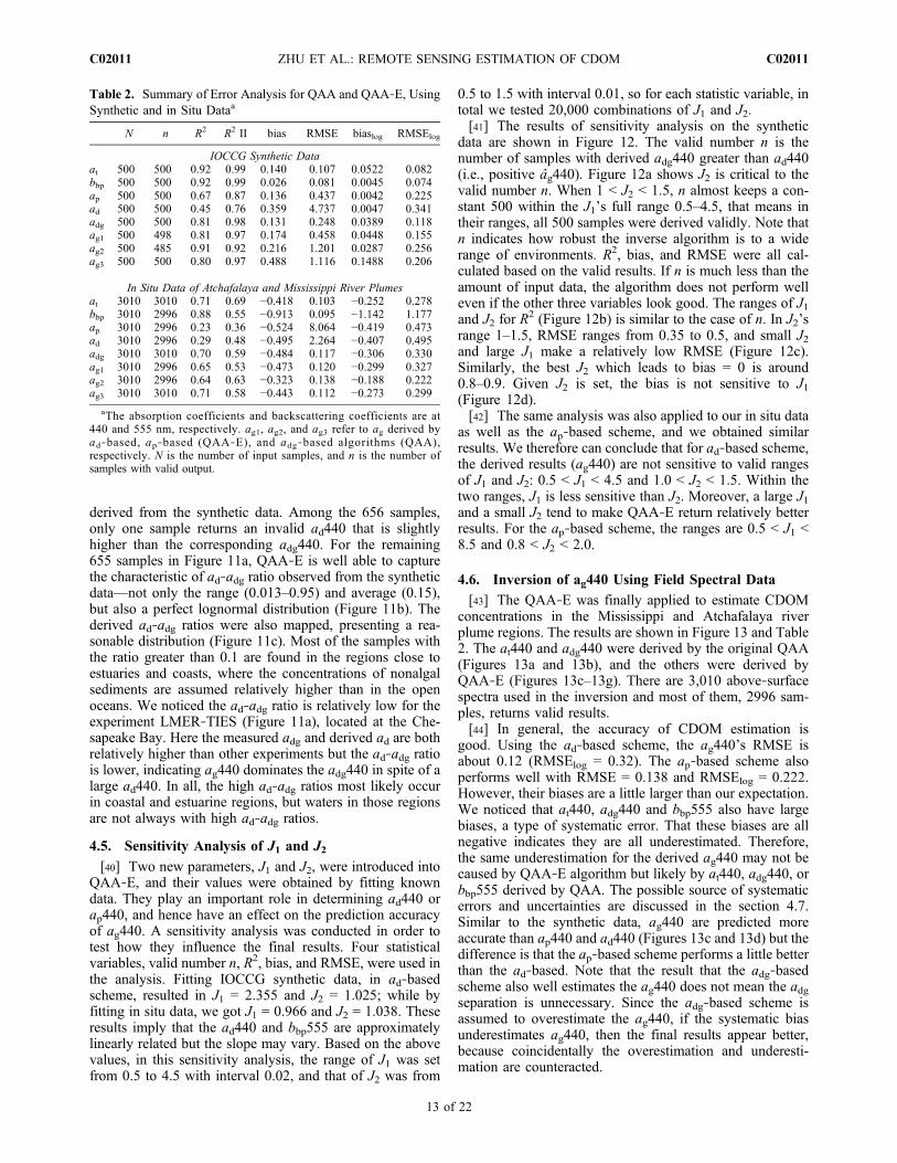
was also used to assess the performance of QAA‐E. Anassumption for adg separation is that ad takes significantproportion in adg. In this study, we set the ratio = 0.1 as thecondition that the adg should be separated. The ratio of thesynthetic data ranges from 0.019 to 0.74 with the average

0.21 and follows a lognormal distribution (Figure 9a). Asthe inversion results, the derived ad‐adg ratio has verysimilar range (from 0.015 to 0.84 with average 0.19) anddistribution (Figure 9b). The detailed comparison (from 0.1to 0.7 with interval 0.02) between the measured and derivedad‐adg ratios also shows they match very well (Figure 9c).[38] We also analyzed the relationship between prediction

error and ad‐adg ratio. The results show that when the ratio islow (0.1–0.4), the error (bias) is also low (Figure 10a); butas the ratio is high, most errors tend to be positive and hencemake a large bias. This phenomenon implies that the QAA‐E works well for moderate ad‐adg ratios, but for very largead‐adg ratios further refinement is required. The very largead‐adg ratio means the sediment concentration is extremelyhigh and in this case the water optical properties are verycomplicated. The remote sensing inversion of ag for suchwater remains challenging.

4.4. QAA‐E Test Using IOCCG in Situ Data

[39] The synthetic data test shows QAA‐E is able toseparate adg440 effectively and hence improve the accuracyof CDOM’s inversion. We also applied QAA‐E to theIOCCG in situ data set which was collected by 11 experi-ments, 656 stations, throughout the global oceans, mostlysampled in coastal areas. This in situ data set only providesadg440 and aph440, so we were unable to validate theaccuracy of the inverted ag440. Nevertheless, we can stillevaluate ad‐adg ratio using QAA‐E‐derived ad440 and insitu adg440. In the test, J1 and J2 were set by the values

Figure 6. Relationships between bbp555 and (a) ad440 and(b) ap440, using synthetic data. Their equations are fittedas ad440 = 2.355bbp

1.025 (R2 = 0.79) and ap440 =6.188bbp

0.953 (R2 = 0.89), respectively.

Figure 7. Relationships between bbp555 and (a) ad440 and(b) ap440, using the measured in situ data. Their equationsare fitted as ad440 = 0.966bbp

1.038 (R2 = 0.965) and ap440 =1.026bbp

0.817 (R2 = 0.954), respectively.

ZHU ET AL.: REMOTE SENSING ESTIMATION OF CDOM C02011C02011

11 of 22

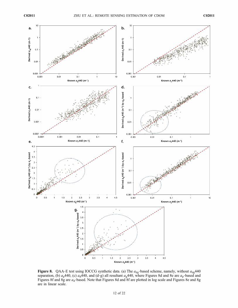
Figure 8. QAA‐E test using IOCCG synthetic data. (a) The adg‐based scheme, namely, without adg440separation, (b) ap440, (c) ad440, and (d‐g) all resultant ag440, where Figures 8d and 8e are ap‐based andFigures 8f and 8g are ad‐based. Note that Figures 8d and 8f are plotted in log scale and Figures 8e and 8gare in linear scale.

ZHU ET AL.: REMOTE SENSING ESTIMATION OF CDOM C02011C02011

12 of 22

derived from the synthetic data. Among the 656 samples,only one sample returns an invalid ad440 that is slightlyhigher than the corresponding adg440. For the remaining655 samples in Figure 11a, QAA‐E is well able to capturethe characteristic of ad‐adg ratio observed from the syntheticdata—not only the range (0.013–0.95) and average (0.15),but also a perfect lognormal distribution (Figure 11b). Thederived ad‐adg ratios were also mapped, presenting a rea-sonable distribution (Figure 11c). Most of the samples withthe ratio greater than 0.1 are found in the regions close toestuaries and coasts, where the concentrations of nonalgalsediments are assumed relatively higher than in the openoceans. We noticed the ad‐adg ratio is relatively low for theexperiment LMER‐TIES (Figure 11a), located at the Che-sapeake Bay. Here the measured adg and derived ad are bothrelatively higher than other experiments but the ad‐adg ratiois lower, indicating ag440 dominates the adg440 in spite of alarge ad440. In all, the high ad‐adg ratios most likely occurin coastal and estuarine regions, but waters in those regionsare not always with high ad‐adg ratios.

4.5. Sensitivity Analysis of J1 and J2[40] Two new parameters, J1 and J2, were introduced into

QAA‐E, and their values were obtained by fitting knowndata. They play an important role in determining ad440 orap440, and hence have an effect on the prediction accuracyof ag440. A sensitivity analysis was conducted in order totest how they influence the final results. Four statisticalvariables, valid number n, R2, bias, and RMSE, were used inthe analysis. Fitting IOCCG synthetic data, in ad‐basedscheme, resulted in J1 = 2.355 and J2 = 1.025; while byfitting in situ data, we got J1 = 0.966 and J2 = 1.038. Theseresults imply that the ad440 and bbp555 are approximatelylinearly related but the slope may vary. Based on the abovevalues, in this sensitivity analysis, the range of J1 was setfrom 0.5 to 4.5 with interval 0.02, and that of J2 was from

0.5 to 1.5 with interval 0.01, so for each statistic variable, intotal we tested 20,000 combinations of J1 and J2.[41] The results of sensitivity analysis on the synthetic

data are shown in Figure 12. The valid number n is thenumber of samples with derived adg440 greater than ad440(i.e., positive âg440). Figure 12a shows J2 is critical to thevalid number n. When 1 < J2 < 1.5, n almost keeps a con-stant 500 within the J1’s full range 0.5–4.5, that means intheir ranges, all 500 samples were derived validly. Note thatn indicates how robust the inverse algorithm is to a widerange of environments. R2, bias, and RMSE were all cal-culated based on the valid results. If n is much less than theamount of input data, the algorithm does not perform welleven if the other three variables look good. The ranges of J1and J2 for R

2 (Figure 12b) is similar to the case of n. In J2’srange 1–1.5, RMSE ranges from 0.35 to 0.5, and small J2and large J1 make a relatively low RMSE (Figure 12c).Similarly, the best J2 which leads to bias = 0 is around0.8–0.9. Given J2 is set, the bias is not sensitive to J1(Figure 12d).[42] The same analysis was also applied to our in situ data

as well as the ap‐based scheme, and we obtained similarresults. We therefore can conclude that for ad‐based scheme,the derived results (ag440) are not sensitive to valid rangesof J1 and J2: 0.5 < J1 < 4.5 and 1.0 < J2 < 1.5. Within thetwo ranges, J1 is less sensitive than J2. Moreover, a large J1and a small J2 tend to make QAA‐E return relatively betterresults. For the ap‐based scheme, the ranges are 0.5 < J1 <8.5 and 0.8 < J2 < 2.0.

4.6. Inversion of ag440 Using Field Spectral Data

[43] The QAA‐E was finally applied to estimate CDOMconcentrations in the Mississippi and Atchafalaya riverplume regions. The results are shown in Figure 13 and Table2. The at440 and adg440 were derived by the original QAA(Figures 13a and 13b), and the others were derived byQAA‐E (Figures 13c–13g). There are 3,010 above‐surfacespectra used in the inversion and most of them, 2996 sam-ples, returns valid results.[44] In general, the accuracy of CDOM estimation is

good. Using the ad‐based scheme, the ag440’s RMSE isabout 0.12 (RMSElog = 0.32). The ap‐based scheme alsoperforms well with RMSE = 0.138 and RMSElog = 0.222.However, their biases are a little larger than our expectation.We noticed that at440, adg440 and bbp555 also have largebiases, a type of systematic error. That these biases are allnegative indicates they are all underestimated. Therefore,the same underestimation for the derived ag440 may not becaused by QAA‐E algorithm but likely by at440, adg440, orbbp555 derived by QAA. The possible source of systematicerrors and uncertainties are discussed in the section 4.7.Similar to the synthetic data, ag440 are predicted moreaccurate than ap440 and ad440 (Figures 13c and 13d) but thedifference is that the ap‐based scheme performs a little betterthan the ad‐based. Note that the result that the adg‐basedscheme also well estimates the ag440 does not mean the adgseparation is unnecessary. Since the adg‐based scheme isassumed to overestimate the ag440, if the systematic biasunderestimates ag440, then the final results appear better,because coincidentally the overestimation and underesti-mation are counteracted.

Table 2. Summary of Error Analysis for QAA and QAA‐E, UsingSynthetic and in Situ Dataa

N n R2 R2 II bias RMSE biaslog RMSElog

IOCCG Synthetic Dataat 500 500 0.92 0.99 0.140 0.107 0.0522 0.082bbp 500 500 0.92 0.99 0.026 0.081 0.0045 0.074ap 500 500 0.67 0.87 0.136 0.437 0.0042 0.225ad 500 500 0.45 0.76 0.359 4.737 0.0047 0.341adg 500 500 0.81 0.98 0.131 0.248 0.0389 0.118ag1 500 498 0.81 0.97 0.174 0.458 0.0448 0.155ag2 500 485 0.91 0.92 0.216 1.201 0.0287 0.256ag3 500 500 0.80 0.97 0.488 1.116 0.1488 0.206

In Situ Data of Atchafalaya and Mississippi River Plumesat 3010 3010 0.71 0.69 −0.418 0.103 −0.252 0.278bbp 3010 2996 0.88 0.55 −0.913 0.095 −1.142 1.177ap 3010 2996 0.23 0.36 −0.524 8.064 −0.419 0.473ad 3010 2996 0.29 0.48 −0.495 2.264 −0.407 0.495adg 3010 3010 0.70 0.59 −0.484 0.117 −0.306 0.330ag1 3010 2996 0.65 0.53 −0.473 0.120 −0.299 0.327ag2 3010 2996 0.64 0.63 −0.323 0.138 −0.188 0.222ag3 3010 3010 0.71 0.58 −0.443 0.112 −0.273 0.299

aThe absorption coefficients and backscattering coefficients are at440 and 555 nm, respectively. ag1, ag2, and ag3 refer to ag derived byad‐based, ap‐based (QAA‐E), and adg‐based algorithms (QAA),respectively. N is the number of input samples, and n is the number ofsamples with valid output.

ZHU ET AL.: REMOTE SENSING ESTIMATION OF CDOM C02011C02011

13 of 22

Figure 9. Compositions of adg(440) (ad‐adg ratio) for (a) measured ratios of IOCCG synthetic data and(b) derived ratios using QAA‐E. (c) The detailed comparison (from 0.1 to 0.7 with interval 0.02) betweenthem.

ZHU ET AL.: REMOTE SENSING ESTIMATION OF CDOM C02011C02011

14 of 22

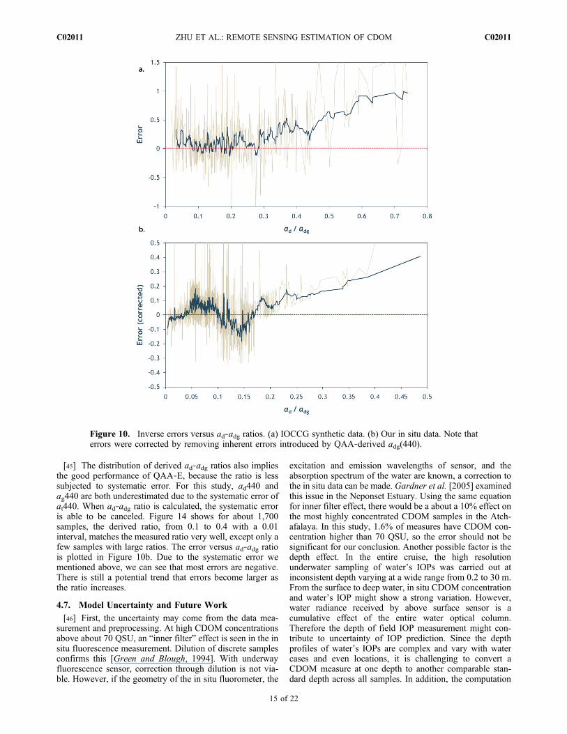
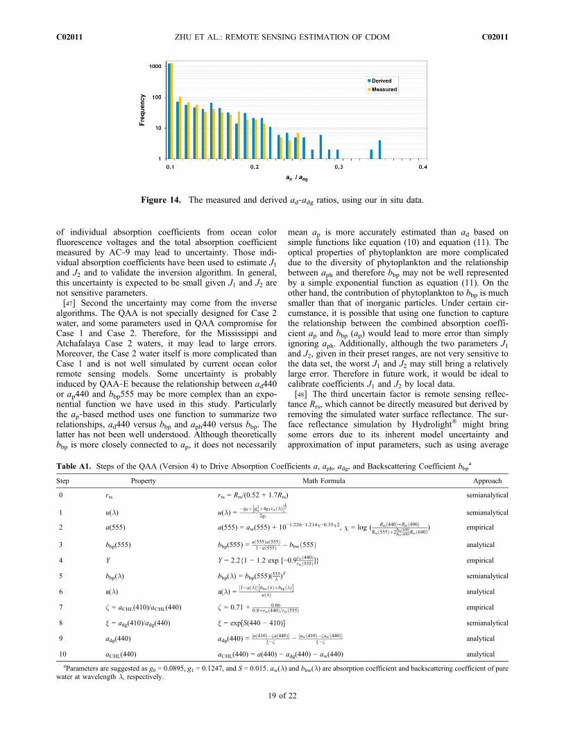
[45] The distribution of derived ad‐adg ratios also impliesthe good performance of QAA‐E, because the ratio is lesssubjected to systematic error. For this study, ad440 andag440 are both underestimated due to the systematic error ofat440. When ad‐adg ratio is calculated, the systematic erroris able to be canceled. Figure 14 shows for about 1,700samples, the derived ratio, from 0.1 to 0.4 with a 0.01interval, matches the measured ratio very well, except only afew samples with large ratios. The error versus ad‐adg ratiois plotted in Figure 10b. Due to the systematic error wementioned above, we can see that most errors are negative.There is still a potential trend that errors become larger asthe ratio increases.

4.7. Model Uncertainty and Future Work

[46] First, the uncertainty may come from the data mea-surement and preprocessing. At high CDOM concentrationsabove about 70 QSU, an “inner filter” effect is seen in the insitu fluorescence measurement. Dilution of discrete samplesconfirms this [Green and Blough, 1994]. With underwayfluorescence sensor, correction through dilution is not via-ble. However, if the geometry of the in situ fluorometer, the

excitation and emission wavelengths of sensor, and theabsorption spectrum of the water are known, a correction tothe in situ data can be made. Gardner et al. [2005] examinedthis issue in the Neponset Estuary. Using the same equationfor inner filter effect, there would be a about a 10% effect onthe most highly concentrated CDOM samples in the Atch-afalaya. In this study, 1.6% of measures have CDOM con-centration higher than 70 QSU, so the error should not besignificant for our conclusion. Another possible factor is thedepth effect. In the entire cruise, the high resolutionunderwater sampling of water’s IOPs was carried out atinconsistent depth varying at a wide range from 0.2 to 30 m.From the surface to deep water, in situ CDOM concentrationand water’s IOP might show a strong variation. However,water radiance received by above surface sensor is acumulative effect of the entire water optical column.Therefore the depth of field IOP measurement might con-tribute to uncertainty of IOP prediction. Since the depthprofiles of water’s IOPs are complex and vary with watercases and even locations, it is challenging to convert aCDOM measure at one depth to another comparable stan-dard depth across all samples. In addition, the computation

Figure 10. Inverse errors versus ad‐adg ratios. (a) IOCCG synthetic data. (b) Our in situ data. Note thaterrors were corrected by removing inherent errors introduced by QAA‐derived adg(440).

ZHU ET AL.: REMOTE SENSING ESTIMATION OF CDOM C02011C02011

15 of 22

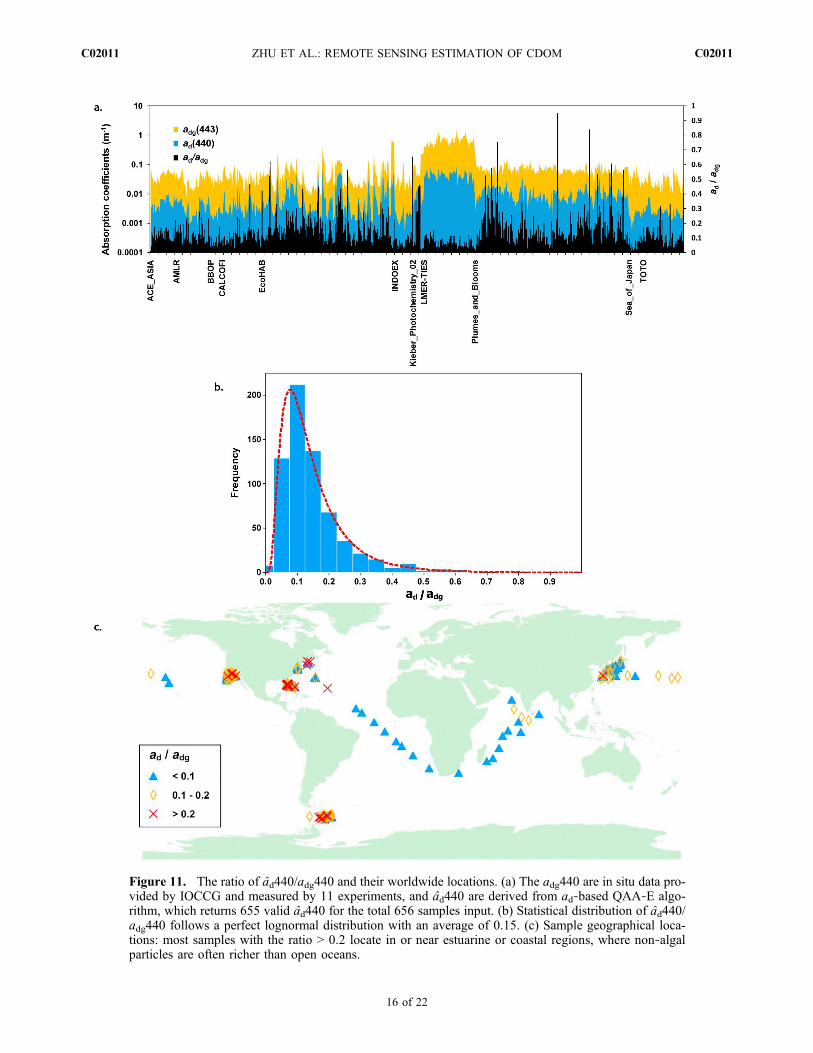
Figure 11. The ratio of âd440/adg440 and their worldwide locations. (a) The adg440 are in situ data pro-vided by IOCCG and measured by 11 experiments, and âd440 are derived from ad‐based QAA‐E algo-rithm, which returns 655 valid âd440 for the total 656 samples input. (b) Statistical distribution of âd440/adg440 follows a perfect lognormal distribution with an average of 0.15. (c) Sample geographical loca-tions: most samples with the ratio > 0.2 locate in or near estuarine or coastal regions, where non‐algalparticles are often richer than open oceans.

ZHU ET AL.: REMOTE SENSING ESTIMATION OF CDOM C02011C02011

16 of 22

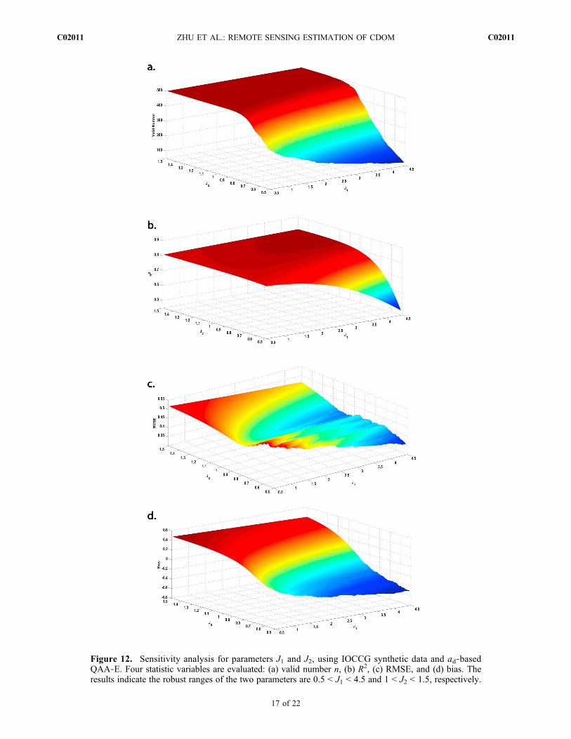
Figure 12. Sensitivity analysis for parameters J1 and J2, using IOCCG synthetic data and ad‐basedQAA‐E. Four statistic variables are evaluated: (a) valid number n, (b) R2, (c) RMSE, and (d) bias. Theresults indicate the robust ranges of the two parameters are 0.5 < J1 < 4.5 and 1 < J2 < 1.5, respectively.

ZHU ET AL.: REMOTE SENSING ESTIMATION OF CDOM C02011C02011

17 of 22

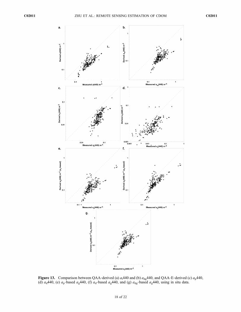
Figure 13. Comparison between QAA‐derived (a) at440 and (b) adg440, and QAA‐E‐derived (c) ap440,(d) ad440, (e) ap‐based ag440, (f) ad‐based ag440, and (g) adg‐based ag440, using in situ data.

ZHU ET AL.: REMOTE SENSING ESTIMATION OF CDOM C02011C02011

18 of 22

of individual absorption coefficients from ocean colorfluorescence voltages and the total absorption coefficientmeasured by AC‐9 may lead to uncertainty. Those indi-vidual absorption coefficients have been used to estimate J1and J2 and to validate the inversion algorithm. In general,this uncertainty is expected to be small given J1 and J2 arenot sensitive parameters.[47] Second the uncertainty may come from the inverse

algorithms. The QAA is not specially designed for Case 2water, and some parameters used in QAA compromise forCase 1 and Case 2. Therefore, for the Mississippi andAtchafalaya Case 2 waters, it may lead to large errors.Moreover, the Case 2 water itself is more complicated thanCase 1 and is not well simulated by current ocean colorremote sensing models. Some uncertainty is probablyinduced by QAA‐E because the relationship between ad440or ap440 and bbp555 may be more complex than an expo-nential function we have used in this study. Particularlythe ap‐based method uses one function to summarize tworelationships, ad440 versus bbp and aph440 versus bbp. Thelatter has not been well understood. Although theoreticallybbp is more closely connected to ap, it does not necessarily

mean ap is more accurately estimated than ad based onsimple functions like equation (10) and equation (11). Theoptical properties of phytoplankton are more complicateddue to the diversity of phytoplankton and the relationshipbetween aph and therefore bbp may not be well representedby a simple exponential function as equation (11). On theother hand, the contribution of phytoplankton to bbp is muchsmaller than that of inorganic particles. Under certain cir-cumstance, it is possible that using one function to capturethe relationship between the combined absorption coeffi-cient ap and bbp (ap) would lead to more error than simplyignoring aph. Additionally, although the two parameters J1and J2, given in their preset ranges, are not very sensitive tothe data set, the worst J1 and J2 may still bring a relativelylarge error. Therefore in future work, it would be ideal tocalibrate coefficients J1 and J2 by local data.[48] The third uncertain factor is remote sensing reflec-

tance Rrs, which cannot be directly measured but derived byremoving the simulated water surface reflectance. The sur-face reflectance simulation by Hydrolight® might bringsome errors due to its inherent model uncertainty andapproximation of input parameters, such as using average

Figure 14. The measured and derived ad‐adg ratios, using our in situ data.

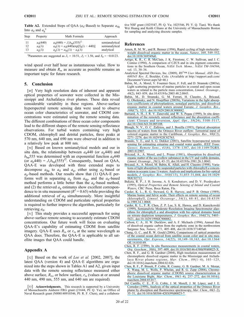
Table A1. Steps of the QAA (Version 4) to Drive Absorption Coefficients a, aph, adg, and Backscattering Coefficient bbpa

Step Property Math Formula Approach

0 rrs rrs = Rrs/(0.52 + 1.7Rrs) semianalytical

1 u(l) u(l) =�g0þ g20þ4g1rrs �ð Þ½ �12

2g1semianalytical

2 a(555) a(555) = aw(555) + 10−1.226−1.214c−0.35c2, c = log ( Rrs 440ð ÞþRrs 490ð ÞRrs 555ð Þþ2Rrs 640ð Þ

Rrs 490ð ÞRrs 640ð Þ) empirical

3 bbp(555) bbp(555) =u 555ð Þa 555ð Þ1�u 555ð Þ � bbw 555ð Þ analytical

4 Y Y = 2.2{1 − 1.2 exp [−0.9rrs 440ð Þrrs 555ð Þ]} empirical

5 bbp(l) bbp(l) = bbp(555)(555� )Y semianalytical

6 a(l) a(l) =1�u �ð Þ½ � bbw �ð Þþbbp �ð Þ½ �

u �ð Þ analytical

7 z = aCHL(410)/aCHL(440) z = 0.71 + 0:060:8þrrs 440ð Þ=rrs 555ð Þ empirical

8 x = adg(410)/adg(440) x = exp[S(440 − 410)] semianalytical

9 adg(440) adg(440) =a 410ð Þ��a 440ð Þ½ �

��� − aw 410ð Þ��aw 440ð Þ½ ���� analytical

10 aCHL(440) aCHL(440) = a(440) − adg(440) − aw(440) analytical

aParameters are suggested as g0 = 0.0895, g1 = 0.1247, and S = 0.015. aw(l) and bbw(l) are absorption coefficient and backscattering coefficient of purewater at wavelength l, respectively.

ZHU ET AL.: REMOTE SENSING ESTIMATION OF CDOM C02011C02011

19 of 22

wind speed over half hour as instantaneous value. How tomeasure and obtain Rrs as accurate as possible remains animportant topic for future research.

5. Conclusion

[49] Very high resolution data of inherent and apparentoptical properties of seawater were collected in the Mis-sissippi and Atchafalaya river plumes. These data revealconsiderable variability in these regions. Above‐surfacehyperspectral remote sensing data were used to observeocean color characteristics of seawater, and CDOM con-centrations were estimated using the remote sensing data.The different combinations of three ocean color componentslead to the different shapes of the remote sensing reflectanceobservations. For turbid waters containing very highCDOM, chlorophyll and detrital particles, three peaks at570 nm, 640 nm, and 690 nm were observed in addition toa relatively low peak at 800 nm.[50] Based on known semianalytical models and our in

situ data, the relationship between ad440 (or ap440) andbbp555 was determined with an exponential function ad440(or ap440) = J1bbp(555)

J2. Consequently, based on QAA,QAA‐E was developed with three extended steps todecompose adg to ad and ag, either using ad‐based orap‐based methods. Our results show that (1) QAA‐E per-forms well in separating ag from adg, and the ad‐basedmethod performs a little better than the ap‐based method,and (2) the retrieved ag estimates show excellent correspon-dence to in situ measurement (R2 = 0.65) while providing theadditional retrieval of ad simultaneously. More insightfulunderstanding on CDOM and particulate optical propertiesis required to further improve the algorithm, particularly forretrieving ad.[51] This study provides a successful approach for using

above‐surface remote sensing to accurately estimate CDOMconcentrations. Our future work will focus on evaluatingQAA‐E’s capability of estimating CDOM from satelliteimagery. QAA‐E uses Rrs or rrs at the same wavelength asQAA does. Therefore, the QAA‐E is applicable to all sat-ellite images that QAA could handle.

Appendix A

[52] Based on the work of Lee et al. [2002, 2007], thelatest QAA (version 4) and QAA‐E algorithms are orga-nized into the steps shown in Tables A1 and A2, given inputdata with the remote sensing reflectance measured eitherabove surface, Rrs, or below surface, rrs (values at or around440 nm, 490 nm, 555 nm, and 640 nm are required).

[53] Acknowledgments. This research is supported by a Universityof Massachusetts Amherst FRG grant (21644, PI: Q. Yu), an Office ofNaval Research grant (N000140910346, PI: R. F. Chen), and a collabora-

tive NSF grant (1025547, PI: Q. Yu; 1025546, PI: Y. Q. Tian). We thankWei Huang and Keith Ciliano at the University of Massachusetts Bostonfor sampling and analyzing discrete samples.

ReferencesAmon, R. M. W., and R. Benner (1994), Rapid cycling of high‐molecular‐weight dissolved organic matter in the ocean, Nature, 369, 549–552,doi:10.1038/369549a0.

Arrigo, K. R., C. R. McClain, J. K. Firestone, C. W. Sullivan, and J. C.Comiso (1994), A comparison of CZCS and in situ pigment concentra-tions in the Southern Ocean, NASA Tech. Memo., NASA TM‐104566,vol. 13, 30–34.

Analytical Spectral Devices, Inc. (2009), RS3™ User Manual, ASD Doc.600545 Rev. E, Boulder, Colo. (Available at http://support.asdi.com/Document/Viewer.aspx?id=46.)

Babin, M., A. Morel, V. Fournier‐Sicre, F. Fell, and D. Stramski (2003a),Light scattering properties of marine particles in coastal and open oceanwaters as related to the particle mass concentration, Limnol. Oceanogr.,48(2), 843–859, doi:10.4319/lo.2003.48.2.0843.

Babin, M., D. Stramski, G. M. Ferrari, H. Claustre, A. Bricaud,G. Obolensky, and N. Hoepffner (2003b), Variations in the light absorp-tion coefficients of phytoplankton, nonalgal particles, and dissolvedorganic matter in coastal waters around Europe, J. Geophys. Res.,108(C7), 3211, doi:10.1029/2001JC000882.

Barnard, A. H., J. R. V. Zaneveld, and W. S. Pegau (1999), In situ deter-mination of the remotely sensed reflectance and the absorption coeffi-cient: Closure and inversion, Appl. Opt., 38(24), 5108–5117,doi:10.1364/AO.38.005108.

Blough, N. V., O. C. Zafiriou, and J. Bonilla (1993), Optical absorptionspectra of waters from the Orinoco River outflow: Terrestrial input ofcolored organic matter to the Caribbean, J. Geophys. Res., 98(C2),2271–2278, doi:10.1029/92JC02763.

Brando, V. E., and A. G. Dekker (2003), Satellite hyperspectral remotesensing for estimating estuarine and coastal water quality, IEEE Trans.Geosci. Remote Sens., 41(6), 1378–1387, doi:10.1109/TGRS.2003.812907.

Bricaud, A., A. Morel, and L. Prieur (1981), Absorption by dissolvedorganic matter of the sea (yellow substance) in the UV and visible domains,Limnol. Oceanogr., 26(1), 43–53, doi:10.4319/lo.1981.26.1.0043.

Bricaud, A., A. Morel, M. Babin, K. Allali, and H. Claustre (1998), Varia-tions of light absorption by suspended particles with chlorophyll a concen-tration in oceanic (case 1) waters: Analysis and implications for bio‐opticalmodels, J. Geophys. Res., 103(C13), 31,033–31,044, doi:10.1029/98JC02712.

Bukata, R. P., J. H. Jerome, A. S. Kondratyev, and D. V. Pozdnyakov(1995), Optical Properties and Remote Sensing of Inland and CoastalWaters, CRC Press, Boca Raton, Fla.

Carder, K. L., R. G. Steward, G. R. Harvey, and P. B. Ortner (1989),Marine humic and fulvic acids: Their effects on remote sensing of oceanchlorophyll , Limnol. Oceanogr. , 34(1), 68–81, doi:10.4319/lo.1989.34.1.0068.

Carder, K. L., F. R. Chen, Z. P. Lee, S. K. Hawes, and D. Kamykowski(1999), Semianalytic Moderate‐Resolution Imaging Spectrometer algo-rithms for chlorophyll a and absorption with bio‐optical domains basedon nitrate‐depletion temperatures, J. Geophys. Res., 104(C3), 5403–5421, doi:10.1029/1998JC900082.

Carlson, C. A., H. W. Ducklow, and A. F. Michaels (1994), Annual fluxof dissolved organic carbon from the euphotic zone in the northwesternSargasso Sea, Nature, 371, 405–408, doi:10.1038/371405a0.

Chang, G. C., and R. W. Gould (2006), Comparisons of optical propertiesof the coastal ocean derived from satellite ocean color and in situ mea-surements, Opt. Express, 14(22), 10,149–10,163, doi:10.1364/OE.14.010149.

Chen, R. F. (1999), In situ fluorescence measurements in coastal waters,Org. Geochem., 30(6), 397–409, doi:10.1016/S0146-6380(99)00025-X.

Chen, R. F., and G. B. Gardner (2004), High‐resolution measurements ofchromophoric dissolved organic matter in the Mississippi and Atchafa-laya River plume regions, Mar. Chem. , 89 (1–4), 103–125,doi:10.1016/j.marchem.2004.02.026.

Chen, R. F., P. Bissett, P. Coble, R. Conmy, G. B. Gardner, M. A. Moran,X. Wang, M. L. Wells, P. Whelan, and R. G. Zepp (2004), Chromo-phoric dissolved organic matter (CDOM) source characterization inthe Louisiana Bight, Mar. Chem., 89(1–4), 257–272, doi:10.1016/j.marchem.2004.03.017.

Del Castillo, C. E., P. G. Coble, J. M. Morell, J. M. López, and J. E.Corredor (1999), Analysis of the optical properties of the Orinoco Riverplume by absorption and fluorescence spectroscopy, Mar. Chem., 66(1–2),35–51, doi:10.1016/S0304-4203(99)00023-7.

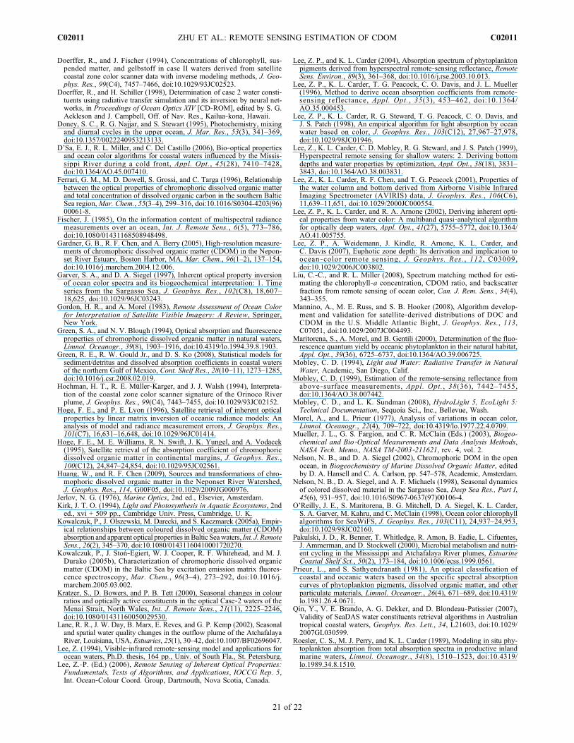
Table A2. Extended Steps of QAA (ad‐Based) to Separate adgInto ad and ag

a

Step Property Math Formula Approach

11 ad(440) ad(440) = J1bbp(555)J2 semianalytical

12 ad(l) ad(l) = ad(440)exp[Sd(l − 440)] semianalytical13 ag(l) ag(l) = adg(l) − ad(l) analytical

aParameters are suggested as J1 = 10.51, J2 = 1.56, and Sd = −0.0123.

ZHU ET AL.: REMOTE SENSING ESTIMATION OF CDOM C02011C02011

20 of 22

Doerffer, R., and J. Fischer (1994), Concentrations of chlorophyll, sus-pended matter, and gelbstoff in case II waters derived from satellitecoastal zone color scanner data with inverse modeling methods, J. Geo-phys. Res., 99(C4), 7457–7466, doi:10.1029/93JC02523.

Doerffer, R., and H. Schiller (1998), Determination of case 2 water consti-tuents using radiative transfer simulation and its inversion by neural net-works, in Proceedings of Ocean Optics XIV [CD‐ROM], edited by S. G.Ackleson and J. Campbell, Off. of Nav. Res., Kailua‐kona, Hawaii.

Doney, S. C., R. G. Najjar, and S. Stewart (1995), Photochemistry, mixingand diurnal cycles in the upper ocean, J. Mar. Res., 53(3), 341–369,doi:10.1357/0022240953213133.

D’Sa, E. J., R. L. Miller, and C. Del Castillo (2006), Bio‐optical propertiesand ocean color algorithms for coastal waters influenced by the Missis-sippi River during a cold front, Appl. Opt., 45(28), 7410–7428,doi:10.1364/AO.45.007410.

Ferrari, G. M., M. D. Dowell, S. Grossi, and C. Targa (1996), Relationshipbetween the optical properties of chromophoric dissolved organic matterand total concentration of dissolved organic carbon in the southern BalticSea region,Mar. Chem., 55(3–4), 299–316, doi:10.1016/S0304-4203(96)00061-8.

Fischer, J. (1985), On the information content of multispectral radiancemeasurements over an ocean, Int. J. Remote Sens., 6(5), 773–786,doi:10.1080/01431168508948498.

Gardner, G. B., R. F. Chen, and A. Berry (2005), High‐resolution measure-ments of chromophoric dissolved organic matter (CDOM) in the Nepon-set River Estuary, Boston Harbor, MA, Mar. Chem., 96(1–2), 137–154,doi:10.1016/j.marchem.2004.12.006.

Garver, S. A., and D. A. Siegel (1997), Inherent optical property inversionof ocean color spectra and its biogeochemical interpretation: 1. Timeseries from the Sargasso Sea, J. Geophys. Res., 102(C8), 18,607–18,625, doi:10.1029/96JC03243.

Gordon, H. R., and A. Morel (1983), Remote Assessment of Ocean Colorfor Interpretation of Satellite Visible Imagery: A Review, Springer,New York.

Green, S. A., and N. V. Blough (1994), Optical absorption and fluorescenceproperties of chromophoric dissolved organic matter in natural waters,Limnol. Oceanogr., 39(8), 1903–1916, doi:10.4319/lo.1994.39.8.1903.

Green, R. E., R. W. Gould Jr., and D. S. Ko (2008), Statistical models forsediment/detritus and dissolved absorption coefficients in coastal watersof the northern Gulf of Mexico, Cont. Shelf Res., 28(10–11), 1273–1285,doi:10.1016/j.csr.2008.02.019.

Hochman, H. T., R. E. Müller‐Karger, and J. J. Walsh (1994), Interpreta-tion of the coastal zone color scanner signature of the Orinoco Riverplume, J. Geophys. Res., 99(C4), 7443–7455, doi:10.1029/93JC02152.

Hoge, F. E., and P. E. Lyon (1996), Satellite retrieval of inherent opticalproperties by linear matrix inversion of oceanic radiance models: Ananalysis of model and radiance measurement errors, J. Geophys. Res.,101(C7), 16,631–16,648, doi:10.1029/96JC01414.

Hoge, F. E., M. E. Williams, R. N. Swift, J. K. Yungel, and A. Vodacek(1995), Satellite retrieval of the absorption coefficient of chromophoricdissolved organic matter in continental margins, J. Geophys. Res.,100(C12), 24,847–24,854, doi:10.1029/95JC02561.

Huang, W., and R. F. Chen (2009), Sources and transformations of chro-mophoric dissolved organic matter in the Neponset River Watershed,J. Geophys. Res., 114, G00F05, doi:10.1029/2009JG000976.

Jerlov, N. G. (1976), Marine Optics, 2nd ed., Elsevier, Amsterdam.Kirk, J. T. O. (1994), Light and Photosynthesis in Aquatic Ecosystems, 2nded., xvi + 509 pp., Cambridge Univ. Press, Cambridge, U. K.

Kowalczuk, P., J. Olszewski, M. Darecki, and S. Kaczmarek (2005a), Empir-ical relationships between coloured dissolved organic matter (CDOM)absorption and apparent optical properties inBaltic Seawaters, Int. J. RemoteSens., 26(2), 345–370, doi:10.1080/01431160410001720270.

Kowalczuk, P., J. Stoń‐Egiert, W. J. Cooper, R. F. Whitehead, and M. J.Durako (2005b), Characterization of chromophoric dissolved organicmatter (CDOM) in the Baltic Sea by excitation emission matrix fluores-cence spectroscopy, Mar. Chem., 96(3–4), 273–292, doi:10.1016/j.marchem.2005.03.002.

Kratzer, S., D. Bowers, and P. B. Tett (2000), Seasonal changes in colourratios and optically active constituents in the optical Case‐2 waters of theMenai Strait, North Wales, Int. J. Remote Sens., 21(11), 2225–2246,doi:10.1080/01431160050029530.

Lane, R. R., J. W. Day, B. Marx, E. Reves, and G. P. Kemp (2002), Seasonaland spatial water quality changes in the outflow plume of the AtchafalayaRiver, Louisiana, USA, Estuaries, 25(1), 30–42, doi:10.1007/BF02696047.

Lee, Z. (1994), Visible‐infrared remote‐sensing model and applications forocean waters, Ph.D. thesis, 164 pp., Univ. of South Fla., St. Petersburg.

Lee, Z.‐P. (Ed.) (2006), Remote Sensing of Inherent Optical Properties:Fundamentals, Tests of Algorithms, and Applications, IOCCG Rep. 5,Int. Ocean‐Colour Coord. Group, Dartmouth, Nova Scotia, Canada.

Lee, Z. P., and K. L. Carder (2004), Absorption spectrum of phytoplanktonpigments derived from hyperspectral remote‐sensing reflectance, RemoteSens. Environ., 89(3), 361–368, doi:10.1016/j.rse.2003.10.013.

Lee, Z. P., K. L. Carder, T. G. Peacock, C. O. Davis, and J. L. Mueller(1996), Method to derive ocean absorption coefficients from remote‐sensing reflectance, Appl. Opt., 35(3), 453–462, doi:10.1364/AO.35.000453.

Lee, Z. P., K. L. Carder, R. G. Steward, T. G. Peacock, C. O. Davis, andJ. S. Patch (1998), An empirical algorithm for light absorption by oceanwater based on color, J. Geophys. Res., 103(C12), 27,967–27,978,doi:10.1029/98JC01946.

Lee, Z., K. L. Carder, C. D. Mobley, R. G. Steward, and J. S. Patch (1999),Hyperspectral remote sensing for shallow waters: 2. Deriving bottomdepths and water properties by optimization, Appl. Opt., 38(18), 3831–3843, doi:10.1364/AO.38.003831.

Lee, Z., K. L. Carder, R. F. Chen, and T. G. Peacock (2001), Properties ofthe water column and bottom derived from Airborne Visible InfraredImaging Spectrometer (AVIRIS) data, J. Geophys. Res., 106(C6),11,639–11,651, doi:10.1029/2000JC000554.

Lee, Z. P., K. L. Carder, and R. A. Arnone (2002), Deriving inherent opti-cal properties from water color: A multiband quasi‐analytical algorithmfor optically deep waters, Appl. Opt., 41(27), 5755–5772, doi:10.1364/AO.41.005755.

Lee, Z. P., A. Weidemann, J. Kindle, R. Arnone, K. L. Carder, andC. Davis (2007), Euphotic zone depth: Its derivation and implication toocean‐color remote sensing, J. Geophys. Res. , 112 , C03009,doi:10.1029/2006JC003802.

Liu, C.‐C., and R. L. Miller (2008), Spectrum matching method for esti-mating the chlorophyll‐a concentration, CDOM ratio, and backscatterfraction from remote sensing of ocean color, Can. J. Rem. Sens., 34(4),343–355.

Mannino, A., M. E. Russ, and S. B. Hooker (2008), Algorithm develop-ment and validation for satellite‐derived distributions of DOC andCDOM in the U.S. Middle Atlantic Bight, J. Geophys. Res., 113,C07051, doi:10.1029/2007JC004493.

Maritorena, S., A. Morel, and B. Gentili (2000), Determination of the fluo-rescence quantum yield by oceanic phytoplankton in their natural habitat,Appl. Opt., 39(36), 6725–6737, doi:10.1364/AO.39.006725.

Mobley, C. D. (1994), Light and Water: Radiative Transfer in NaturalWater, Academic, San Diego, Calif.

Mobley, C. D. (1999), Estimation of the remote‐sensing reflectance fromabove‐surface measurements, Appl. Opt., 38(36), 7442–7455,doi:10.1364/AO.38.007442.

Mobley, C. D., and L. K. Sundman (2008), HydroLight 5, EcoLight 5:Technical Documentation, Sequoia Sci., Inc., Bellevue, Wash.

Morel, A., and L. Prieur (1977), Analysis of variations in ocean color,Limnol. Oceanogr., 22(4), 709–722, doi:10.4319/lo.1977.22.4.0709.

Mueller, J. L., G. S. Fargion, and C. R. McClain (Eds.) (2003), Biogeo-chemical and Bio‐Optical Measurements and Data Analysis Methods,NASA Tech. Memo., NASA TM‐2003‐211621, rev. 4, vol. 2.

Nelson, N. B., and D. A. Siegel (2002), Chromophoric DOM in the openocean, in Biogeochemistry of Marine Dissolved Organic Matter, editedby D. A. Hansell and C. A. Carlson, pp. 547–578, Academic, Amsterdam.

Nelson, N. B., D. A. Siegel, and A. F. Michaels (1998), Seasonal dynamicsof colored dissolved material in the Sargasso Sea, Deep Sea Res., Part I,45(6), 931–957, doi:10.1016/S0967-0637(97)00106-4.

O’Reilly, J. E., S. Maritorena, B. G. Mitchell, D. A. Siegel, K. L. Carder,S. A. Garver, M. Kahru, and C. McClain (1998), Ocean color chlorophyllalgorithms for SeaWiFS, J. Geophys. Res., 103(C11), 24,937–24,953,doi:10.1029/98JC02160.

Pakulski, J. D., R. Benner, T. Whitledge, R. Amon, B. Eadie, L. Cifuentes,J. Ammerman, and D. Stockwell (2000), Microbial metabolism and nutri-ent cycling in the Mississippi and Atchafalaya River plumes, EstuarineCoastal Shelf Sci., 50(2), 173–184, doi:10.1006/ecss.1999.0561.

Prieur, L., and S. Sathyendranath (1981), An optical classification ofcoastal and oceanic waters based on the specific spectral absorptioncurves of phytoplankton pigments, dissolved organic matter, and otherparticulate materials, Limnol. Oceanogr., 26(4), 671–689, doi:10.4319/lo.1981.26.4.0671.

Qin, Y., V. E. Brando, A. G. Dekker, and D. Blondeau‐Patissier (2007),Validity of SeaDAS water constituents retrieval algorithms in Australiantropical coastal waters, Geophys. Res. Lett., 34, L21603, doi:10.1029/2007GL030599.

Roesler, C. S., M. J. Perry, and K. L. Carder (1989), Modeling in situ phy-toplankton absorption from total absorption spectra in productive inlandmarine waters, Limnol. Oceanogr., 34(8), 1510–1523, doi:10.4319/lo.1989.34.8.1510.

ZHU ET AL.: REMOTE SENSING ESTIMATION OF CDOM C02011C02011

21 of 22

Sandidge, J. C., and R. J. Holyer (1998), Coastal bathymetry from hyper-spectral observations of water radiance, Remote Sens. Environ., 65(3),341–352, doi:10.1016/S0034-4257(98)00043-1.

Sathyendranath, S. (Ed.) (2000), Remote Sensing of Ocean Colour inCoastal, and Other Optically‐Complex, Waters, IOCCG Rep. 3, Int.Ocean‐Colour Coord. Group, Dartmouth, Nova Scotia, Canada.

Sathyendranath, S., F. E. Hoge, T. Platt, and R. N. Swift (1994), Detectionof phytoplankton pigments from ocean color: Improved algorithms, Appl.Opt., 33(6), 1081–1089, doi:10.1364/AO.33.001081.

Sathyendranath, S., G. Cota, V. Stuart, H. Maass, and T. Platt (2001),Remote sensing of phytoplankton pigments: A comparison of empiricaland theoretical approaches, Int. J. Remote Sens., 22(2–3), 249–273,doi:10.1080/014311601449925.

Shooter, D., and P. Brimblecombe (1989), Dimethylsulfide oxidation in theocean, Deep Sea Res., Part A, 36(4), 577–585, doi:10.1016/0198-0149(89)90007-1.

Siegel, D. A., and A. F. Michaels (1996), Quantification of non‐algal lightattenuation in the Sargasso Sea: Implications for biogeochemistry andremote sensing, Deep Sea Res. , Part II , 43(2–3), 321–345,doi:10.1016/0967-0645(96)00088-4.

Siegel, D. A., S. Maritorena, N. B. Nelson, D. A. Hansell, and M. Lorenzi‐Kayser (2002), Global distribution and dynamics of colored dissolvedand detrital organic materials, J. Geophys. Res., 107(C12), 3228,doi:10.1029/2001JC000965.

Stedmon, C. A., S. Markager, M. Søndergaard, T. Vang, A. Laubel, N. H.Borch, and A. Windelin (2006), Dissolved organic matter (DOM) exportto a temperate estuary: Seasonal variations and implications of land use,Estuaries Coasts, 29(3), 388–400, doi:10.1007/BF02784988.

U.S. Army Corps of Engineers (2008), The Atchafalaya Basin Project,report, New Orleans, La. (Available at http://www.mvn.usace.army.mil/pao/bro/AtchafalayaBasinProject.pdf.)

Valentine, R. L., and R. G. Zepp (1993), Formation of carbon monoxidefrom the photodegradation of terrestrial dissolved organic carbon in natu-ral waters, Environ. Sci. Technol., 27(2), 409–412, doi:10.1021/es00039a023.

Van Der Woerd, H. J., and R. Pasterkamp (2008), HYDROPT: A fast andflexible method to retrieve chlorophyll‐a from multispectral satellite ob-servations of optically complex coastal waters, Remote Sens. Environ.,112(4), 1795–1807, doi:10.1016/j.rse.2007.09.001.

Vodacek, A., N. V. Blough, M. D. DeGrandpre, E. T. Peltzer, and R. K.Nelson (1997), Seasonal variation of CDOM and DOC in the MiddleAtlantic Bight: Terrestrial inputs and photooxidation, Limnol. Oceanogr.,42(4), 674–686, doi:10.4319/lo.1997.42.4.0674.

Yentsch, C. S. (1962), Measurement of visible light absorption by particu-late matter in the ocean, Limnol. Oceanogr., 7(2), 207–217, doi:10.4319/lo.1962.7.2.0207.

Yu, Q., Y. Q. Tian, R. F. Chen, A. Liu, G. B. Gardner, and W. N. Zhu(2010), Functional linear analysis for estimating riverine CDOM incoastal environment using in situ hyperspectral data, Photogramm.Eng. Remote Sens., 76(10), 1147–1158.

Zhan, H., S. Ping, and C. Chen (2005), A Bayesian based quasi‐analyticalalgorithm for retrieval of inherent optical properties from ocean color,Chin. Sci. Bull., 50(23), 2770–2777, doi:10.1360/982004-828.

R. F. Chen, G. B. Gardner, and Y. Q. Tian, Department ofEnvironmental, Earth and Ocean Sciences, University of MassachusettsBoston, 100 Morrissey Blvd., Boston, MA 02125, USA.Q. Yu and W. Zhu, Department of Geosciences, University of

Massachusetts Amherst, 611 N. Pleasant St., Amherst, MA 01003, USA.(qyu@geo.umass.edu)

ZHU ET AL.: REMOTE SENSING ESTIMATION OF CDOM C02011C02011

22 of 22