Journal of Contaminant Hydrology 138–139 (2012) 22–39

Contents lists available at SciVerse ScienceDirect

Journal of Contaminant Hydrology

j ourna l homepage: www.e lsev ie r .com/ locate / jconhyd

Stochastic evaluation of mixing-controlled steady-state plume lengths intwo-dimensional heterogeneous domains

Olaf A. Cirpka a,⁎, Massimo Rolle a,b, Gabriele Chiogna c, Felipe P.J. de Barros d, Wolfgang Nowak e

a University of Tübingen, Center for Applied Geoscience, Hölderlinstr, 12, 72074 Tübingen, Germanyb Stanford University, Department of Civil and Environmental Engineering, Jerry Yang & Akiko Yamazaki Environment & Energy Building, 473 Via Ortega, Stanford,CA 94305, USAc University of Trento, Department of Civil and Environmental Engineering, Via Mesiano 77, 38123 Trento, Italyd Dept. of Geotechnical Engineering and Geosciences, Jordi Girona 1-3, 08034 Barcelona, Spaine University of Stuttgart, Institute of Modeling Hydraulic and Environmental Systems, LH2/SimTech, Pfaffenwaldring 5a, 70569 Stuttgart, Germany

a r t i c l e i n f o

⁎ Corresponding author. Tel.: +49 7071 2978928; fE-mail address: olaf.cirpka@uni-tuebingen.de (O.A

0169-7722/$ – see front matter © 2012 Elsevier B.V. Adoi:10.1016/j.jconhyd.2012.05.007

a b s t r a c t

Article history:Received 14 January 2012Received in revised form 2 April 2012Accepted 23 May 2012Available online 23 June 2012

We study plumes originating from continuous sources that require a dissolved reactionpartner for their degradation. The length of such plumes is typically controlled by transversemixing. While analytical expressions have been derived for homogeneous flow fields,incomplete characterization of the hydraulic conductivity field causes uncertainty inpredicting plume lengths in heterogeneous domains. In this context, we analyze the effectsof three sources of uncertainty: (i) The uncertainty of the effective mixing rate along the plumefringes due to spatially varying flow focusing, (ii) the uncertainty of the volumetric dischargethrough (and thus total mass flux leaving) the source area, and (iii) different parameteriza-tions of the Darcy-scale transverse dispersion coefficient. The first two are directly related toheterogeneity of hydraulic conductivity. In this paper, we derive semi-analytical expressionsfor the probability distribution of plume lengths at different levels of complexity. The resultsare compared to numerical Monte Carlo simulations. Uncertainties in mixing and in the sourcestrength result in a statistical distribution of possible plume lengths. For unconditional randomhydraulic conductivity fields, plume lengths may vary by more than one order of magnitudeeven for moderate degrees of heterogeneity. Our results show that the uncertainty ofvolumetric flux through the source is the most relevant contribution to the variance of theplume length. The choice of different parameterizations for the local dispersion coefficientleads to differences in the mean estimated plume length.

© 2012 Elsevier B.V. All rights reserved.

Keywords:Transverse dispersionGroundwater transportMixing-controlled reactionsStochastic subsurface hydrology

1. Introduction

The study of dilution and mixing processes occurring inthe direction perpendicular to main groundwater flow is ofprimary importance when assessing natural attenuation ofpollutants in the subsurface. Typical groundwater plumes oforganic contaminants, originating from continuous sources

ax: +49 7071 295059.. Cirpka).

ll rights reserved.

(e.g., NAPL spills), can approach a steady state with finitesolute mass within the domain (e.g., Mace et al., 1997;Widemeier et al., 1999). This is achieved by a dynamicequilibrium between the contaminant mass released from thesource and its destruction by (bio)degradationprocesses (Fraseret al., 2008). Under these conditions, transverse dispersionrepresents the principal mixing mechanism that facilitatesreactions of the contaminant with reactants transported in theambient groundwater.

If the kinetics of the degrading reaction are sufficiently fast,the mixing at the plume fringes is the limiting step for the

23O.A. Cirpka et al. / Journal of Contaminant Hydrology 138–139 (2012) 22–39

degradation of the contaminant. These conditions have beenobserved at a number of high-resolution monitored field sites(e.g., Davis et al., 1999; Prommer et al., 2006, 2009; Thornton etal., 2001) as well as in detailed laboratory experiments at boththe Darcy scale (e.g., Bauer et al., 2009a, 2009b; Huang et al.,2003) and at the pore scale (e.g.,Willinghamet al., 2008; Zhanget al., 2010). Mixing-controlled biodegradation was alsoinvestigated in a number of modeling studies (e.g., Cirpka etal., 1999a; Ham et al., 2004; Liedl et al., 2005).

In practical applications such as risk analysis, naturalattenuation assessment or remediation, it is important toassess the maximum length of the plume to be expected.Analytical solutions (Cirpka et al., 2006; Liedl et al., 2005, 2011)as well as empirical relationships based on numerical simula-tions (Maier and Grathwohl, 2006) have been proposed toestimate the length of steady-state contaminant plumes inhomogeneous or upscaled porous media. In two-dimensionalhomogeneous settings, the basic result is that the length of theplume scales linearlywith the squaredwidth of the plume at itsorigin, and inversely with the transverse dispersion coefficient.Predicting plume lengths becomes more challenging inheterogeneous porous media, where the spatial variability ofthe hydraulic conductivity plays a pivotal role in solutetransport and mixing (see Rubin, 2003, Chapter 7).

If the exact spatial distribution of hydraulic conductivity wasknown, the length of a mixing-controlled plume could beevaluated by numerical simulation. Such studies have beenperformed by Werth et al. (2006) and Chiogna et al. (2011a,b),among others, to demonstrate the net effect of heterogeneity onsolute mixing and mixing-controlled reactions. In reality,however, the exact distribution is not known and a geostatisticalcharacterization, quantifying variability and uncertainty oflog-hydraulic conductivity, may be the best information avail-able. Under such conditions, probabilistic tools become neces-sary to evaluate expected values and uncertainties of predictions(e.g., Rubin, 2003). While extensive Monte Carlo simulations arealways a possible way to obtain empirical distributions ofprediction outcomes, (semi)analytical expressions give moreinsight into the principles of uncertainty propagation or into therole of individual processes and can be evaluated at lowercomputational costs.

In this study, we investigate steady-state, mixing-controlledreactive transport in 2-D heterogeneous porous media. Wequantify how the uncertainty in predicting the length ofcontaminant plumes is related to three main sources ofuncertainty:

1. The uncertainty of effective transverse mixing along theplume fringes in heterogeneous media;

2. The uncertainty of the water flux through (and thus thetotal contaminant mass flux leaving) the source, caused bythe heterogeneity within and around the source area;

3. The parameterization of the local transverse dispersioncoefficient.

Spatial variability of hydraulic conductivity has two majoreffects on steady-state mixing-controlled plumes. The first oneis related to the effective transverse dispersion along theplume fringe. In high-conductivity zones, streamlines arefocused, decreasing the transverse diffusion length, whichleads to enhancedmass transfer across streamlines (e.g.,Werthet al., 2006). Likewise, if a plume fringe passes through a

low-conductivity zone, where the transverse diffusion length isincreased, themass transfer across streamlines is slowed down.The importance of high-conductivity inclusions as hot spotsof transverse mixing and mixing-controlled reactions havebeen demonstrated in several experimental studies (e.g., Baueret al., 2009a; Cirpka et al., 1999d; Rolle et al., 2009). Innumerical experiments, Werth et al. (2006) showed thatthe average net effect of heterogeneity on transverse solutemixing is an enhancement, implying that the decrease oftransverse mixing in low-conductivity zones is overbalancedby the increase in high-conductivity zones. For an individualplume in a heterogeneous porous medium, however, it is quitepossible that its fringe mainly comes to lie in low-conductivityzones such that the plume is longer than in the homogeneouscase.

For conservative transport in two-dimensional heteroge-neousmedia, Cirpka et al. (2011b) reformulated the advection–dispersion equation in streamline coordinates and expressedeffective transverse mixing in terms of transverse spatialmoments in these coordinates, thus removing the effects ofstreamline meandering. They performed a rigorous first-orderanalysis of effective transverse mixing for two-dimensionalheterogeneous media with second-order stationary, statistical-ly isotropic, multi-Gaussian log-hydraulic conductivity fields,assuming uniform-in-the-mean flow. They derived analyticalexpressions for mean effective transverse dispersion, whichwas confirmed to be enhanced in heterogeneous media.They could predict the uncertainty in the degree of effectivetransverse mixing stemming from the uncertainty ofvelocity and flow focusing along the plume fringe. For thelength of mixing-controlled plumes, it should be expectedthat the mean effective transverse mixing coefficient relatesto the mean plume length, and the uncertainty of effectivemixing can explain the uncertainty of plume length to somedegree.

The second effect of heterogeneity on the length ofmixing-controlled plumes is via the volumetric flux throughthe source zone. If the source zone is located in a high-conductivity zone, the local velocities are higher, and a largervolumetric flux is loadedwith the contaminant than in the casewhen the source zone is located in a low-conductivity zone. Alarger volumetric flux through the source zone leads to a widerplume once the streamlines defocus again, and this in turnleads to a longer plume. Thus, the uncertainty of hydraulicconductivity in the source zone contributes to the uncertaintyof plume lengths. This has already been investigated in astochastic framework by de Barros and Nowak (2010), whoused Scheidegger's (1961) parameterization for local dispersionand neglected the uncertainty of effective transverse mixingalong the plume fringe. Within the context of optimizing siteinvestigation campaigns, Nowak et al. (2010) and Leube et al.(2012) found that, even for far-field prediction of contaminantconcentrations, intensive investigations of the hydraulicconditions at and around the source are highly important.This suggests, to some extent, that the total volumetric fluxthrough the source (and hence the total mass flux leavingfixed-concentration sources) might be the dominant originof uncertainty to address the overall fate of contaminantplumes under the investigated conditions.

Finally, the choice of the local-scale dispersion modelcan affect the plume length prediction. Recent laboratory

24 O.A. Cirpka et al. / Journal of Contaminant Hydrology 138–139 (2012) 22–39

bench-scale experiments (Chiogna et al., 2010) have shownthat a compound-specific, nonlinear parameterization of localtransverse dispersion agrees better with experimental resultsperformed in homogeneous porous media than the traditionalmodel of Scheidegger (1961). Scheidegger's (1961) modelassumes a linear dependence of the transverse dispersioncoefficient on the flow velocity. The model proposed byChiogna et al. (2010) accounts for incomplete mixing in thepore channels of the solidmatrix, resulting in a less-than-lineardependence on flow velocity and a non-negligible influence ofmolecular diffusion on transverse dispersion also at highvelocities. Chiogna et al. (2011a) have demonstrated bynumerical experiments that the compound dependence ofmechanical transverse dispersion is indeed relevant for reactivetransport at field scales. The cited studies imply that the modelchoice for the local transverse dispersion is also relevant forconservative and mixing-controlled reactive transport, even athigher groundwater velocities.

In this paper, we analyze the combined effects of these threedifferent uncertainty sources when estimating the length ofcontaminant plumes in heterogeneous porous media, and toquantify which is the most relevant one. Our results are limitedto steady-state flow and transport conditions in two dimensions.To achieve our goals, we follow the approach by Cirpka et al.(2011b) to transform from Cartesian coordinates to streamlinecoordinates. This removes the effects of streamline meandering.Extensions to three dimensions will not be straightforward,because transforming to streamline coordinates is not trivial inthree dimensions. Still, the key findings on the mechanisms atwork in two dimensions can provide valuable insights even forthree-dimensional systems.

We derive semi-analytical expressions for the statistics ofplume length. They are formally limited to 1st-order theory(e.g., Dagan, 1984; Gelhar and Axness, 1983), and are basedon the Scheidegger (1961) parameterization for local trans-verse dispersion. The analytical expressions are compared tothe results from numerical Monte Carlo simulations. In thenumerical simulations, we also test the influence of differentmodels of local transverse dispersion that cannot be consid-ered in the semi-analytical expressions.

Table 1Parameterizations of transverse dispersion Dt used in this study.

I Non-linear (Chiogna et al.,2010):

Dt;i ¼ qθ

dffiffiffiffiffiffiffiffiffiffiffiffiffiffiPeiþ123

p þ Dp;i with Pei ¼ qdθDm;i

;

II Linear with K-dependentdispersivity:

Dt;i ¼ qθ at

ffiffiffiffiK

pþ Dp;i

III Linear with constantdispersivity (Scheidegger,1961):

Dt;i ¼ qθ αt þ Dp;i

2. Problem formulation

2.1. Flow and transport

We consider two-dimensional, confined, divergence-freegroundwater flow at steady state in an infinite domain withmean hydraulic gradient J [−] oriented in the longitudinalx1-direction. The hydraulic conductivity K [LT−1] is assumedto be locally isotropic. Then, the hydraulic head φ [L] and thestream-function ψ [L2T−1] meet the following set of ellipticpartial differential equations:

∇⋅ K∇φð Þ ¼ 0; ð1Þ

∇⋅ 1K∇ψ

� �¼ 0; ð2Þ

subject to:

∇φ ¼ −J0

� �;∇ψ ¼ −q2

q1

� �; ð3Þ

in which the overbar denotes a spatial average, and q=[q1,q2]T

[LT−1] is the specific-discharge vector following Darcy's law:

q ¼ −K∇φ: ð4Þ

Steady-state transport of a reactive compound i isdescribed by the advection–dispersion–reaction equation:

q⋅∇ci−∇⋅ θDi∇cið Þ ¼ ri; ð5Þ

in which ci [ML−3] is the concentration of compound i, θ [−]is the porosity, Di [L2T−1] is the dispersion tensor, which maydiffer from compound to compound, and ri [ML−3T−1] is thereaction rate of compound i. The principal directions of thedispersion tensor coincide at each point with the localdirection of flow and perpendicular to it, such that (e.g.,Bear, 1972, Chapter 10):

Di ¼q⊗qq⋅q Dℓ;i−Dt;i

� �þ IDt;i; ð6Þ

in which q⊗q and q⋅q are the matrix and scalar products ofq with itself, respectively, and I is the identity matrix,whereas Dℓ;i [L2T−1] and Dt,i [L2T−1] are the longitudinaland transverse dispersion coefficients of compound i,respectively.

In steady-state transport, the effects of the longitudinaldispersion coefficient Dℓ;i become negligible for Peℓ ¼ x�v=Dℓ > 30 (Domenico, 1987; Domenico and Robbins, 1985;Ham et al., 2004; Srinivasan et al., 2007), whereas Dt,i

becomes important when boundary conditions enforcelateral concentration gradients. For Dt,i, we consider theparameterizations listed in Table 1, in which αt [L] is aconstant, compound-independent hydromechanical trans-verse dispersivity, at [L1/2T1/2] is a proportionality constantrelating the transverse dispersivity to the square-root of K(Hazen, 1892), Dp,i [L2T−1] is the pore diffusion coefficient ofcompound i, differing from the corresponding moleculardiffusion coefficient Dm,i [L2T−1] by the tortuosity of theporous medium, d is a characteristic grain diameter, and Pei[−] is the grain Péclet number of compound i.

While the flow domain is infinite, the domain for transportis semi-infinite with the line x1=0 being the inflow boundary.We assume a line source at the inflow boundary over theinjection width ws [L] centered about x2=0. In the source, theconcentration is fixed to the inflow concentration ci

in [ML−3],

25O.A. Cirpka et al. / Journal of Contaminant Hydrology 138–139 (2012) 22–39

whereas it is fixed to the ambient concentration ciamb [ML−3] at

the remaining part of the inflow boundary:

ci 0; x2ð Þ ¼ cini if−ws

2≤x2≤

ws

2cambi otherwise

;

8<: ð7Þ

All other boundaries are infinitely far away and do notinfluence the concentration distribution.

2.2. Mixing-controlled reaction

We consider an instantaneous (or sufficiently fast) andirreversible reaction of a plume-borne compound A (i.e., adissolved organic contaminant) and a reactant B (i.e., adissolved electron acceptor) introduced in parallel, formingthe reaction product C:

f AAþ f BB→f CC; ð8Þ

in which fi [−] is the stoichiometric coefficient of compoundi. At the inflow boundary, compounds A and B are perfectlyseparated between the source area and the ambient flow,because B is being fully depleted in the part of the flow thattravels through the source area:

cinA > 0; cambB > 0; camb

A ¼ cinB ¼ cambC ¼ cinC ¼ 0: ð9Þ

The reaction rates of the individual compounds are in thestoichiometric ratio of the reaction:

rA ¼ −f Ar; rB ¼ −f Br; rC ¼ f Cr; ð10Þ

in which r [ML−3T−1] is an effective Darcy-scale reaction rate,which depends among other influences on velocity-dependentpore-scale mixing of compounds A and B, and thus varies inspace. In the limit of an instantaneous, irreversible, completereaction of compounds A and B, r is implicitly defined byenforcing that the reactants A and B do not coexist:

cAcB ¼ 0; ð11Þ

and spatial variation of r becomes irrelevant.

3. Predicting the length of contaminant plumes forcompound-independent dispersion coefficients

Here, we consider the case that all dispersion coefficientsare identical, DA=DB=DC=D. Then, the reactive-speciesconcentrations cA, cB, and cC are uniquely defined by themixing ratio X [−] between compounds A and B, whichformally undergoes conservative transport:

q⋅∇X−∇⋅ θD∇Xð Þ ¼ 0; ð12Þ

X 0; x2ð Þ ¼ 1 if−ws

2≤x2≤

ws

20 otherwise

:

(ð13Þ

The mixing ratio X describes the volumetric fraction ofplume−borne water in the mixture with ambient water.

The concentration of both reactants A and B is zero, cA=cB=0, where the mixing ratio X [−] of the plume waterequals the critical mixing ratio Xcrit [−]. The critical mixing

ratio is determined solely by the stoichiometry of thereaction (Cirpka and Valocchi, 2007):

Xcrit ¼f Ac

ambB

f BcinA þ f Ac

ambB

: ð14Þ

In the present study, we are interested in the length L [L]of a steady-state mixing-controlled plume in heterogeneousmedia. The plume length L is defined as the maximumdistance from the source in the x1-direction, at which theplume-borne compound A can still be found. This is thelargest x1-coordinate that can be found along the contour lineX(x1,x2)=Xcrit.

3.1. Plume length in homogeneous domains

The following analytical result for the plume length L inuniform two-dimensional flow with a line injection perpen-dicular to the flow is taken from Cirpka et al. (2006). It hasbeen derived from the analytical solution of steady-statetwo-dimensional advective–dispersive transport by Domenicoand Palciauskas (1982), whose validity is limited by theconditions given by Srinivasan et al. (2007):

L ¼ qw2s

16Dtθ erf−1 Xcritð Þ 2 ð15Þ

in which erf−1(Xcrit) is the inverse error function with argumentXcrit.

It may be worth noting that other geometric settings formixing-controlled reactive transport result in slightly differ-ent expressions with identical scaling of L with Dtθ/q and ws

in 2-D (e.g., Ham et al., 2004; Liedl et al., 2005), and similarscaling in 3-D (Liedl et al., 2011).

3.2. Plume length in heterogeneous settings

In heterogeneous porous media, K (and thus the velocity)varies in space. A convenient way to deal with spatiallyvariable advection is to change from Cartesian to streamlinecoordinates. By definition, streamline coordinates are alignedat each point in space with the local direction of flow andperpendicular to it. The advection–dispersion equation forthe mixing ratio X in streamline coordinates reads as (Cirpkaet al., 2011b; Rahman et al., 2005):

− q2

K∂X∂φ− q

K∂∂φ θDℓ

qK∂X∂φ

� �−q

∂∂ψ θDtq

∂X∂ψ

� �¼ 0; ð16Þ

X x1 ¼ 0;ψð Þ ¼ 1 if−Qs

2≤ψ≤Qs

20 otherwise

;

(ð17Þ

inwhich the stream-function valueψ is chosen to be zero in thecenter of the plume source, and Qs [L2T−1] is the cumulativedischarge passing through the line source. To be consistentwith the Cartesian problem, the boundary condition of Eq. (17)is expressed as function of the longitudinal Cartesian coordi-nate x1 and the stream-function value ψ rather than in φ and ψ.Also, we will keep several important terms expressed in theoriginal coordinate x1 rather than in φ. This corresponds to the

26 O.A. Cirpka et al. / Journal of Contaminant Hydrology 138–139 (2012) 22–39

approximation Δx1≈−JΔφ already used in Cirpka et al.(2011b).

The most important effect of switching to streamline co-ordinates is that advective transport becomes a one-dimensionalprocess always perpendicular to ψ, simplifying the followinganalysis. An increase in the transverse second central moment ofX in streamline coordinates indicates that the solute flux isdistributed over a larger volumetric flux, which is an adequatemeasure of transverse mixing (Chiogna et al., 2011b; Cirpka etal., 2011b; Rolle et al., 2009). In contrast, the transverse secondcentralmoment in Cartesian coordinates is affected by squeezingand stretching of the plume due to streamlinemeandering. Fig. 1shows the simulated distribution of themixing ratio in Cartesianand streamline coordinates, plotted for a random realization ofheterogeneity. Quite obviously, all effects of plume meandering,squeezing, and stretching are removed by switching intostreamline coordinates. In streamline coordinates, the plumeeven appears to be fairly symmetric, although the transversedispersion term θDtq appearing in Eq. (17) may vary differentlyat the two fringes of the plume.

In steady-state transport, the effect of Dℓ on the concentra-tion distribution is negligible at a sufficiently long distancefrom the source, such that the corresponding transport termcan be neglected in the following (see discussion in Cirpka etal., 2011b). A key assumption in the following analysis is thatthe analytical concentration distribution for the homogenousvelocity field (Domenico and Palciauskas, 1982) is a good

Fig. 1. Mixing ratio X for constant injection at steady state in a heterogeneousdomain, comparison between Cartesian (A) and streamline (B) coordinates.

approximation to the heterogeneous case if we replace thetransverse coordinate y by the stream-function value ψ:

X x1;ψð ÞðÞ ¼ 12

erfψ−ψc þ Qs=2ffiffiffiffiffiffiffiffiffiffiffiffiffiffiffiffiffiffi

2w2δ x1ð Þ

q0B@

1CA−erf

ψ−ψc−Qs=2ffiffiffiffiffiffiffiffiffiffiffiffiffiffiffiffiffiffi2w2

δ x1ð Þq

0B@

1CA

264

375;ð18Þ

in which x1 [L] is the longitudinal distance, ψc is the centerposition of the plume in stream-function values, and wδ

2(x1)[L4T−2] is the squared width of the plume fringe instream-function values.

For a line-source injection over the volumetric flux Qs, thesquared fringe width wδ

2(x1) in stream-function values is thedifference of the normalized transverse second-centralmomentm2c

(ψ) of X(ψ,x1) in stream-function values at distancex1 to the one at the source:

ψc x1ð Þ ¼ ∫þ∞−∞ψ� X x1;ψð Þdψ

Qsð19Þ

w2δ x1ð Þ ¼ m ψð Þ

2c x1ð Þm ψð Þ

0

−m ψð Þ2c 0ð Þm ψð Þ

0 Þ

¼ ∫þ∞−∞ψ

2 � X x1;ψð ÞdψQs

−ψ2c x1ð Þ−Q2

s

12: ð20Þ

We test the validity of Eq. (18) in the case of steady-statetransport in heterogeneous domains by numerical experi-ments discussed in Appendix D. If Eq. (18) is correct, themaximum value of the mixing-ratio within a transverseprofile is uniquely defined by the volumetric flux through thesource Qs and the fringe width wδ in stream-function values:

max X ψð jQs;w2δ x1ð Þ

� �Þ ¼ erf

Qs

2ffiffiffiffiffiffiffiffiffiffiffiffiffiffiffiffiffiffi2w2

δ x1ð Þq

0B@

1CA: ð21Þ

The validity of this equation for steady-state plumes inheterogeneous aquifers is tested empirically, also in Appendix D.

Now we reconsider the instantaneous reaction of com-pounds A and B to C. All compounds are assumed to undergothe same transverse dispersion. As outlined above, theconcentrations of both A and B are zero when the mixingratio equals its critical value X=Xcrit (Eq. (14)). In the spatialsetting, the contour line X=Xcrit marks the boundary of thereactive plume. We now look at the transverse profile of X atsome distance x1. If the maximum value of X within thatprofile according to Eq. (21) is larger than Xcrit, thencompound A still exists at that distance x1. This implies thatthe end of the plume has not yet been reached, i.e., that theplume length L must be larger than x1. Conversely, ifmax(X(ψ|Qs,wδ

2(x1)))bXcrit, compound A does not exist anymore at that distance, and hence Lbx1. Ifmax(X(ψ|Qs,wδ

2(x1)))=Xcrit, the distance x1 is exactly equal to the plume length (see alsoChiogna et al., 2011b).

Thus, for the instantaneous reaction considered here, thelength L [L] of the plume is implicitly given as:

max X ψð jQs;w2δ Lð Þ

� �Þ ¼ Xcrit; ð22Þ

27O.A. Cirpka et al. / Journal of Contaminant Hydrology 138–139 (2012) 22–39

⇒w2δ Lð Þ ¼ Q2

s

8 erf−1 Xcritð Þ� �2 ; ð23Þ

which may be simplified in notation to:

w2δ Lð Þ ¼ A2Q2

s ; ð24Þ

with

A ¼ 1ffiffiffi8

perf−1 Xcritð Þ : ð25Þ

Our next step to derive the reactive plume-lengthstatistics is to approximate the statistics of wδ

2. Cirpka et al.(2011b) analyzed wδ

2 in heterogeneous domains for the caseof a point injection rather than the line injection consideredhere. They obtained the following approximation:

w2δ Lð Þ ¼ 2θJ∫L

0KDtdx1; ð26Þ

which requires low to mild levels of heterogeneity and anarrow fringe width. In Appendix E, we empirically testwhether this approximation of wδ

2 (derived for a pointinjection) also holds for the line source setup considered inour current study. If this is the case, and if the relationshipbetween wδ

2 and the maximum of the mixing ratio within atransverse profile can reasonably be approximated by Eq. (21),we can derive the statistical distribution of the plume length Lfor given source strength Qs from the statistics of wδ

2 at allpotential distances x1. This is discussed in Section 4.2.2.

The second uncertain quantity, determining the length ofthe reactive plume, is the total volumetric discharge Qs

passing through the source zone:

Qs ¼ ∫þws=2−ws=2

q1dx2 ¼ ψ ws=2ð Þ−ψ −ws=2ð Þ: ð27Þ

For a given geometric source width ws, the volume flux Qs

passing through the source depends on the exact distributionof hydraulic conductivity in and around the source area. deBarros and Nowak (2010) analyzed the statistical propertiesof stream-function differences in isotropic heterogeneousdomains. If only (geo)statistical information about thehydraulic conductivity field exists, Qs is subject to significantuncertainty. The latter authors showed that this substantiallyaffects the plume length, plume dispersion and overallconcentration distribution.

4. Stochastic setting

4.1. Definitions

In order to make use of existing analytical expressions, weassume that the logarithmic hydraulic conductivity Y=lnK isa second-order stationary, multi-Gaussian random spacefunction. Under these conditions, the following relationshold:

K xð Þ ¼ Kgexp Y ′ xð Þh i

; ð28Þ

Y ′ xð Þ ¼ 0∀x; ð29Þ

Y ′ x þ hð ÞY ′ xð Þ ¼ CYY hð Þ∀x; ð30Þ

σ2Y ¼ CYY 0ð Þ ¼ Y ′2

; ð31Þ

in which Kg [L/T] is the spatially uniform geometric mean ofhydraulic conductivity, Y′ [−] is the zero mean fluctuation ofY, ⟨⟩ denotes the ensemble average of the argument, h [L] is aspatial separation vector, CYY(h) [−] is the auto-covariancefunction of Y, and σY

2 [−] is the field variance of Y. In ourwork, we report results for an isotropic exponential covari-ance function CYY(h):

CYY hð Þ ¼ σ2Yexp − hj j

λ

� �ð32Þ

with the integral scale, or correlation length, λ [L].For this covariance function, first-order expressions for

the statistical mean and variance of the source strength Qs

and for the squared width wδ2(x1) of the plume fringe in

stream-function values have been derived by de Barros andNowak (2010) and Cirpka et al. (2011b), respectively. Themean values, denoted by μ with a corresponding subscript,are given by:

μQs¼ wsJKg ; ð33Þ

μw2δx1ð Þ ¼ 2θJKgD

eqt x1; ð34Þ

with

Deqt ¼ ⟨KDt⟩

Kg: ð35Þ

Here, Dteq [L2T−1] is the equivalent transverse dispersion

coefficient that quantifies actual transverse mixing, i.e., theprobability of a solute particle to cross a given number ofstreamlines within a given period of time.

The expressions provided in Eq. (36) below give anoverview of equivalent transverse dispersion coefficients forisotropic heterogeneous media with exponential covariancefunction when applying the three different parameteriza-tions of local transverse dispersion given in Table 1 (Cirpka etal., 2011b):

I : Deqt ≈ 1þ 1

2σ2

Y

� �Dp þ 1þ 1:56σ2

Y þ 1:92σ4Y

� �KgJθ

dffiffiffiffiffiffiffiffiffiffiffiffiffiffiffiffiffiffiffiffiPeþ 123

p ;

with d≈ffiffiffiffiffiffiKg

q� 0:01 m1=2s1=2

h i; Pe ¼ KgJd

θDm

II : Deqt ≈ 1þ 1

2σ2

Y

� �Dp þ 1þ 1

4σ2

Y þ 3:88σ4Y

� �atK

3=2g Jθ

;

III : Deqt ≈ 1þ 1

2σ2

Y

� �Dp þ 1þ σ2

Y þ 0:7σ4Y

� �αtKgJθ

;

ð36Þ

Existing results for the variance of Qs and wδ2(x1) are

reproduced in Appendices A and B. In Appendix C, we deriveat first order the covariance between Qs and wδ

2(x1). Based onevidence of previous studies, both Qs and wδ

2 are assumed toapproximately follow a log-normal distribution (Cirpka et al.,2011a,b; de Barros and Nowak, 2010). The log-normal

28 O.A. Cirpka et al. / Journal of Contaminant Hydrology 138–139 (2012) 22–39

probability density function (pdf) for a generic variable u isdefined as:

pu ¼ 1uσ lnu

ffiffiffiffiffiffi2π

p exp − lnu−μ lnuð Þ22σ2

lnu

!: ð37Þ

Here, pu is the pdf of u, whereas μlnu and σlnu2 are the mean

and variance of ln(u). The statistical moments of a Gaussianlog-quantity ln(u) can be computed from the mean μu andvariance σu

2 of the non-logarithmic quantity u via thefollowing well-known relations:

μ lnu ¼ lnμ2uffiffiffiffiffiffiffiffiffiffiffiffiffiffiffiffiffi

σ2u þ μ2

u

q0B@

1CA; ð38Þ

σ2lnu ¼ ln 1þ σ2

u

μ2u

!: ð39Þ

In the following, we will use the approximate pdfs pQsand

pwδ2(x1) together with the relationship of Eq. (24), which is

exact only for homogeneous conditions, to approximate pdfsof the plume length L for different levels of complexity.

4.2. Statistical distribution of the plume length L

As we mentioned in the introduction, we wish to investi-gate the relative importance of three sources of uncertainty inthe estimation of the length of a reactive plume. One is due tothe alternative possible parameterizations of the local trans-verse dispersion coefficient (see Table 1). The other twopotential sources of uncertainty are due to the heterogeneousnature of the porous matrix: Fluctuations in the velocity fieldlead to uncertainty of (i) the source strength and (ii) theeffective transverse dispersion coefficient. Therefore, in astochastic framework, it is natural to identify four mainscenarios to be investigated: The case where we consider thetransverse dispersion coefficient to be known, but the sourcestrength is uncertain (Section 4.2.1); the casewhere the sourcestrength is known but the transverse dispersion coefficient isuncertain (Section 4.2.2); and the two cases where bothquantities are uncertain but their uncertainties are considereduncorrelated (Section 4.2.3) or correlated (Section 4.2.4),respectively.

4.2.1. Statistical distribution of the plume length L for uncertainsource strength Qs and deterministic transverse mixingcoefficient Dt

eq

Our simplest statistical distribution of the plume length Lassumes that the only cause of uncertainty is the volume fluxpassing through the source. This is the same setting asanalyzed by de Barros and Nowak (2010). In this model, weassume that effective transverse mixing can be describeddeterministically by Dt

eq according to the expressions provid-ed in Eq. (36), neglecting the associated uncertainty. Then,we obtain the deterministic relationship L(Qs):

L ¼ Q2s

16Deqt JKgθ erf−1 Xcritð Þ 2 ; ð40Þ

expressing that the plume length L scales with the squaredsource strength Qs

2. Because pQsis assumed to be log-normal,

the resulting pdf pL for the plume length L is also log-normal(see also de Barros and Nowak, 2010, Section 4.1), withcoefficients:

μ lnL ¼ 2μ lnQs−ln 16Deq

t JKgθ erf−1 Xcritð Þ� �2� �

; ð41Þ

σ lnL ¼ 2σ lnQs: ð42Þ

The assumption of a constant local (e.g., hydromechani-cal) dispersion coefficient is often found in the literature inorder to simplify the mathematical approach to the problem,(e.g., Le Borgne et al., 2010). However, in our case weconsider a constant effective transverse dispersion coefficient.This coefficient is not merely a local coefficient, but alreadyincludes the average effect of mixing enhancement producedby flow focusing in high permeability inclusions.

4.2.2. Statistical distribution of plume length L for deterministicsource strength Qs and uncertain transverse mixing

The second model assumes that the volumetric flux Qs

through the source is perfectly known, as was assumed in thestudies of Chiogna et al. (2011a,b), but the effective transversemixing coefficient Dt

eq (or equivalently: the squared fringewidth wδ

2(x1) in stream-function values) is considered uncer-tain.

This scenario corresponds to the case where the source zonehas been well characterized, or to field transport experimentsperformed at research sites by emplacing a contaminant sourcein the subsurface at a well-investigated location (e.g., Fraser etal., 2008; King and Barker, 1999). Under these conditions, theprobability that the plume reaches only a length L or shorter isidentical to the probability that wδ

2 at distance L is A2Qs2 or

larger (see Eq. (24)). This can be expressed as a mapping of thecumulative distribution functions (cdfs) Pwδ

2(L)→PL:

PL x1ð Þ ¼ 1−Pw2δ x1ð Þ A2Q2

s

� �: ð43Þ

Note that, even though pwδ2(x1) is assumed log-normal for

all values of x1, the resulting distribution pL is not log-normalbecause the statistical parameters of pwδ

2(x1) change withdistance x1.

4.2.3. Statistical distribution of the plume length L for uncertainsource strength Qs and uncorrelated uncertain transverse mixing

In the third model, we account for uncertainty in bothsource strength Qs and in the cumulative transverse mixingwδ

2. However, we do not yet consider a potential correlationbetween these two properties. In this context, Eq. (43) maybe seen as conditional cdf PL(x1|Qs) of the plume length forgiven Qs, and the unconditional cdf PL(x1) is obtained bysimple marginalization:

PL x1ð Þ ¼ ∫∞0 1−Pw2

δ x1ð Þ A2Q2s

� �h ipQs

Qsð ÞdQs; ð44Þ

in which pQs(Qs) is the pdf of Qs, here considered to be

independent of wδ2(x1).

29O.A. Cirpka et al. / Journal of Contaminant Hydrology 138–139 (2012) 22–39

This case is presented for the sake of completeness only.In fact, it is unlikely that uncertainty related to the sourcestrength and to the cumulative transverse mixing can beconsidered uncorrelated, since they both stem from theheterogeneity of the same flow field.

4.2.4. Statistical distribution of the plume length L for uncertainsource strength Qs and correlated uncertain transverse mixing

The fourth and potentially most complete model in thispaper accounts for correlated uncertainty of the source strengthQs and of the squared fringe width wδ

2(x1) in stream-functioncoordinates. These quantities should be correlated for smallvalues of x1, because both Qs and wδ

2(x1) depend on thehydraulic-conductivity distribution in the direct vicinity of thesource. In Appendix C, we derive to first order in σY thecovariance Cwδ

2(x1),Qs, assuming Scheidegger's (1961) model oflocal transverse dispersion with constant dispersivity αt.

To obtain the plume-length statistics, we replace themarginal probability Pwδ

2(x1) of the squared fringe width inEq. (44) by the conditional one, Pwδ

2(x1)|Qs:

PL x1ð Þ ¼ ∫∞0 1−Pw2

δ x1ð ÞjQs A2Q2s

� �h ipQs

Qsð ÞdQs ð45Þ

The statistical moments of the conditional distributionPwδ

2(x1)|Qs may be approximated to first order by linearizeduncertainty propagation:

μw2δ x1ð ÞjQs ¼ μw2

δ x1ð Þ þCw2

δ x1ð Þ;Qs

σ2Qs

Qs−μQs

� �ð46Þ

σw2δ x1ð ÞjQs

2 ¼ σ2w2

δ x1ð Þ−C2w2

δ x1ð Þ;Qs

σ2Qs

ð47Þ

in which μQsand μwδ

2(x1) are the unconditional expected valuesof Qs and wδ

2(x1), respectively, σQs

2 and σwδ2(x1)

2 are thecorresponding unconditional variances, Cwδ

2(x1),Qs is the covari-ance between Qs and wδ

2(x1), whereas μwδ2(x1)|Qs and σwδ

2(x1)|Qs2

are the conditional expected value and variance of wδ2(x1). We

further assume that the conditional distribution Pwδ2(x1)|Qs

remains log-normal like the unconditional distribution Pwδ2(x1).

5. Numerical test cases

5.1. Numerical implementation

In order to test the analytical expressions derived aboveand to assess the simultaneous influence of different sourcesof uncertainty on the statistics of reactive plume lengths, weperform numerical Monte Carlo simulations. We consider a2-D, rectangular domain that is discretized into squareelements for flow simulations. We use an isotropic exponen-tial covariance model of the log-conductivity to generate1000 realizations of log-conductivity by the method ofDietrich and Newsam (1993).

Groundwater flow is solved by the Galerkin Finite ElementMethod with bilinear elements, with the same code as used inNowak and Cirpka (2006) andNowak et al. (2008). The left andright boundaries are considered Dirichlet boundaries for

hydraulic head, whereas the top and bottom boundaries areconsidered no-flow boundaries. For steady-state transport, weconstruct streamline-oriented grids according to themethod ofCirpka et al. (1999b), and apply the Finite Volume Method onstreamline-oriented grids (Cirpka et al., 1999c). The contam-inant line source is located at some distance from the leftboundary of the domain, oriented into the x2-direction, and hasthe width ws. Placing the source away from the inlet boundaryis done in order to minimize the effect of the fixed-headboundary condition on the velocity field experienced by thesolute plume. All parameters are listed in Table 2, and theymaybe considered typical values reported in literature (e.g., Freeze,1975).

We use different models for local transverse dispersion,discussed in detail in Section 5.2. Because hydraulic hetero-geneity is explicitly resolved, the values of the dispersioncoefficients Dℓ;i and Dt,i represent pore-scale dispersion, andtheir magnitudes correspond to values found in laboratoryexperiments (Delgado, 2006; Olsson and Grathwohl, 2007).That is, they are significantly smaller then typical effectivefield scale values (Prommer et al., 2009; Thierrin andKitanidis, 1994), since the latter represent upscaled valuesthat account for the effects of heterogeneity above the Darcyscale on solute mixing.

The inlet concentration for the contaminant and theambient concentration for the electron acceptor are set tounity, while the concentration for the product C is zeroeverywhere along the inflow boundary. The stoichiometriccoefficients for the contaminant fA and the product fC are 1,while for the species B, we select fB=0.1. These values arechosen to meet an Xcrit of 0.9, which is required to limit thenumber of realizations where the plumes extend beyond theboundary of our numerical domain.

5.2. Different setups for local transverse dispersion in numericaltest cases

The goals of our numerical simulations are twofold. First,we test the assumptions made our analytical solutions byconsidering comparable scenarios. Second, we investigatecases for which no analytical solution is available.

In total, we perform three different sets of Monte Carlosimulations including six relevant cases representative ofreactive transport scenarios with an increasing degree ofsimplification. In the first set, we focus on the differentcompound-specific aqueous diffusion and local transversedispersion coefficients of the reaction partners (denoted asCase 1, no analytical solution is available for this scenario). Inthe second set of simulations, we focus our attention on theparameterizations of the local transverse dispersion coeffi-cient (Cases 2, 3 and 4) while assuming identical coefficientsfor all species. These simulations are performed considering afixed geometry for the source, therefore displaying avariability both in the source strength and in transversemixing along the plume fringes. The outcomes of the MonteCarlo analysis of Cases 2, 3 and 4 can be compared to theanalytical solution provided by Eq. (40) in Section 4.2.1 whenapplying the different parameterizations therein. The resultsobtained for Case 4, where the linear Scheidegger (1961)parameterization is used in the numerical model, can becomparedwith the analytical solutions provided in Sections 4.2.3

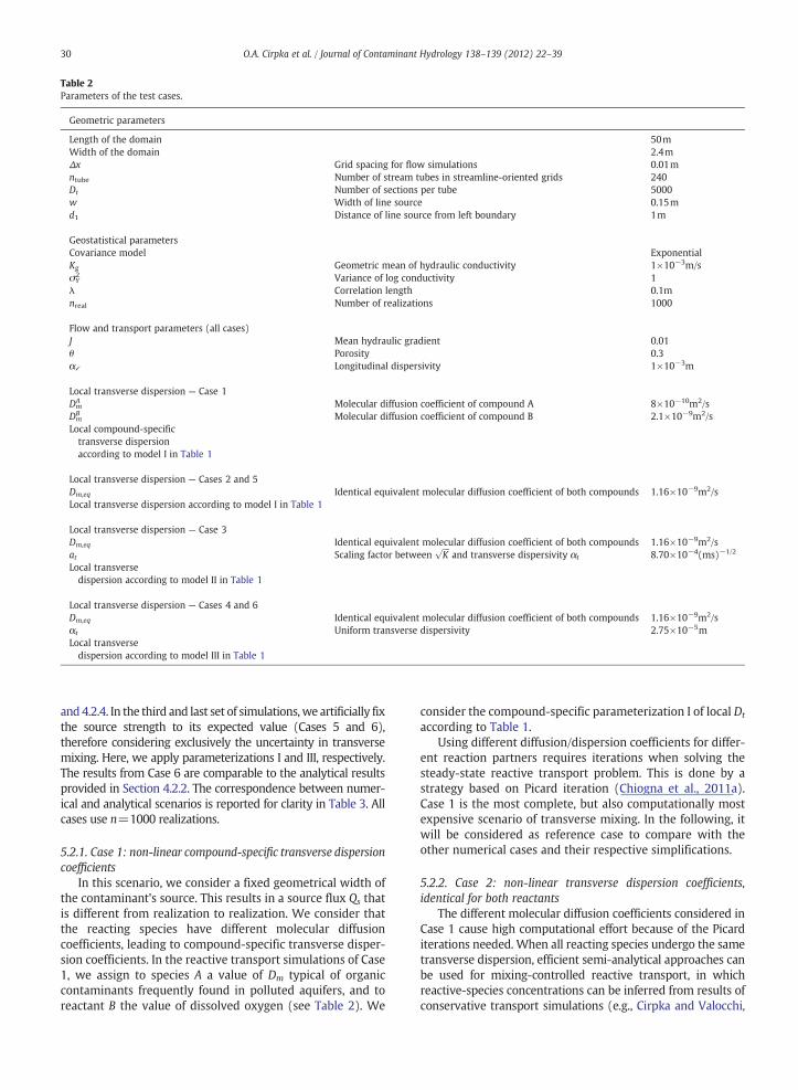
Table 2Parameters of the test cases.

Geometric parameters

Length of the domain 50mWidth of the domain 2.4mΔx Grid spacing for flow simulations 0.01mntube Number of stream tubes in streamline-oriented grids 240Dt Number of sections per tube 5000w Width of line source 0.15md1 Distance of line source from left boundary 1m

Geostatistical parametersCovariance model ExponentialKg Geometric mean of hydraulic conductivity 1×10−3m/sσY2 Variance of log conductivity 1

λ Correlation length 0.1mnreal Number of realizations 1000

Flow and transport parameters (all cases)J Mean hydraulic gradient 0.01θ Porosity 0.3αℓ Longitudinal dispersivity 1×10−3m

Local transverse dispersion — Case 1DmA Molecular diffusion coefficient of compound A 8×10−10m2/s

DmB Molecular diffusion coefficient of compound B 2.1×10−9m2/s

Local compound-specifictransverse dispersionaccording to model I in Table 1

Local transverse dispersion — Cases 2 and 5Dm,eq Identical equivalent molecular diffusion coefficient of both compounds 1.16×10−9m2/sLocal transverse dispersion according to model I in Table 1

Local transverse dispersion — Case 3Dm,eq Identical equivalent molecular diffusion coefficient of both compounds 1.16×10−9m2/sat Scaling factor between

ffiffiffiffiK

pand transverse dispersivity αt 8.70×10−4(ms)−1/2

Local transversedispersion according to model II in Table 1

Local transverse dispersion — Cases 4 and 6Dm,eq Identical equivalent molecular diffusion coefficient of both compounds 1.16×10−9m2/sαt Uniform transverse dispersivity 2.75×10−5mLocal transversedispersion according to model III in Table 1

30 O.A. Cirpka et al. / Journal of Contaminant Hydrology 138–139 (2012) 22–39

and 4.2.4. In the third and last set of simulations,we artificially fixthe source strength to its expected value (Cases 5 and 6),therefore considering exclusively the uncertainty in transversemixing. Here, we apply parameterizations I and III, respectively.The results from Case 6 are comparable to the analytical resultsprovided in Section 4.2.2. The correspondence between numer-ical and analytical scenarios is reported for clarity in Table 3. Allcases use n=1000 realizations.

5.2.1. Case 1: non-linear compound-specific transverse dispersioncoefficients

In this scenario, we consider a fixed geometrical width ofthe contaminant's source. This results in a source flux Qs thatis different from realization to realization. We consider thatthe reacting species have different molecular diffusioncoefficients, leading to compound-specific transverse disper-sion coefficients. In the reactive transport simulations of Case1, we assign to species A a value of Dm typical of organiccontaminants frequently found in polluted aquifers, and toreactant B the value of dissolved oxygen (see Table 2). We

consider the compound-specific parameterization I of local Dt

according to Table 1.Using different diffusion/dispersion coefficients for differ-

ent reaction partners requires iterations when solving thesteady-state reactive transport problem. This is done by astrategy based on Picard iteration (Chiogna et al., 2011a).Case 1 is the most complete, but also computationally mostexpensive scenario of transverse mixing. In the following, itwill be considered as reference case to compare with theother numerical cases and their respective simplifications.

5.2.2. Case 2: non-linear transverse dispersion coefficients,identical for both reactants

The different molecular diffusion coefficients considered inCase 1 cause high computational effort because of the Picarditerations needed. When all reacting species undergo the sametransverse dispersion, efficient semi-analytical approaches canbe used for mixing-controlled reactive transport, in whichreactive-species concentrations can be inferred from results ofconservative transport simulations (e.g., Cirpka and Valocchi,

Table 3Comparison between numerical scenarios and available analytical solutions.

Set of simulations Numerical scenario Corresponding analytical solutions

1. Compoundspecific

Case 1: Non-linear compound specific transverse dispersion coefficient No analytical solution

2. Comparison of localparameterizations

Case 2: Non-linear transverse dispersion coefficients, identical for both reactants No analytical solution, comparison with Eq. (40)Case 3: Linear transverse dispersion coefficients with K-dependent dispersivity No analytical solution, comparison with Eq. (40)Case 4: Linear transverse dispersion coefficients with uniformdispersivity

Sections 4.2.3, 4.2.4 and comparison withEq. (40)

3. Fixed sourcestrength

Case 5: Non-linear transverse dispersion coefficients, identical for both reactants No analytical solutionCase 6: Linear transverse dispersion coefficients with uniform dispersivity Section 4.2.2

31O.A. Cirpka et al. / Journal of Contaminant Hydrology 138–139 (2012) 22–39

2007; De Simoni et al., 2005; De Simoni et al., 2007; Liedl et al.,2005; Liedl et al., 2011). Thus, in Case 2 we introduce anequivalent, fictitious aqueous diffusion coefficient (Dm,eq) thatis identical for all reacting species. We substitute thiscoefficient into parameterization I, which was also used inCase 1. The resulting parameterization of the local transversedispersion coefficient used in Case 2 reads as:

Dt ¼ Dp;eq þqθ

dffiffiffiffiffiffiffiffiffiffiffiffiffiffiffiffiffiffiffiffiffiffiffiffiffiffiffiffiffi123þ Peeq� �r ð48Þ

in which Dp,eq is the equivalent pore diffusion coefficient andPeeq=v×d/Dm,eq is the equivalent Péclet number. The value forthe equivalent aqueous diffusion coefficient is chosen such thatthe statistical distributions of plume lengths fromCase 2 fit bestto those observed in Case 1.

5.2.3. Case 3: linear transverse dispersion coefficients withK-dependent dispersivity

In this scenario, we introduce an additional simplificationby making the mechanical transverse dispersion termindependent of the diffusive properties of the transportedcompounds. We use the linear parameterization II of local Dt

(Table 1), where the mechanical dispersion term spatiallyvaries with the flow velocity and – via the grain size – withhydraulic conductivity. In order to obtain comparable valuesfor the local transverse dispersion coefficient (i.e., samemeanvalue as in Case 2) we consider an equivalent diffusioncoefficient Dm,eq for Case 3 with at defined as:

at ¼1

100ffiffiffiffiffiffiffiffiffiffiffiffiffiffiffiffiffiffiffiffiffiffiffiffiffiffiffiffiffiffi123þ Peeq� �r m1=2s1=2

h ið49Þ

in which

Peeq ¼ d qθDm;eq

ð50Þ

and

d ¼ffiffiffiffiffiffiKg

q100

m1=2s1=2h i

ð51Þ

Therefore, the local transverse dispersion coefficient forCase 3 reads as:

Dt ¼ Dp;eq þqθat

ffiffiffiffiK

pð52Þ

5.2.4. Case 4: linear transverse dispersion coefficients withuniform dispersivity

For the most simplified case, we consider the classicallinear parameterization of Scheidegger (1961) for transversedispersion with uniform dispersivity αt (parameterization IIIin Table 1). Here, the transverse mechanical dispersion termvaries exclusively with flow velocity. Similarly to Case 3, weneed to define a dispersivity αt that yields comparable valuesof local Dt:

αt ¼dffiffiffiffiffiffiffiffiffiffiffiffiffiffiffiffiffiffiffiffiffiffiffiffiffiffiffiffiffiffi

123þ Peeq� �r ð53Þ

whered and Peeq are defined as in Case 3 and αt is constant inspace. Therefore, the local transverse dispersion coefficientused in this scenario is:

Dt ¼ Dp;eq þqθαt ð54Þ

This simplifyingmodel is also the basis for the semi-analyticalexpression of the plume-length pdf derived in Section 4.2.1.

5.2.5. Cases 5 and 6: fixed source strength Qs

In these final scenarios, we fix the volumetric flux throughthe source for two parameterizations of the local transversedispersion coefficient Dt. With respect to Dt, Case 5 iscomparable with Case 2, in which we consider non-linearparameterization I in Table 1 with the same Dp

eq as in Case 2,whereas in Case 6 we apply the local Dt parameterization III,that is, the parameterization of Scheidegger (1961) withuniform dispersivity αt. This is equivalent to Case 4, but witha fixed value of Qs. Based on these two extra cases andcomparison to Cases 2 and 4, we can distinguish the effects ofthe uncertain source strength Qs and of the uncertaintransverse mixing along the plume fringe on the statisticaldistribution of the plume length. To this end, we adapt thegeometrical width of the source in each realization in such away that the volumetric flux through the source linecorresponds to the expected value of the previous four

Fig. 2. Spatial distribution of the reaction partners A, B and the product C in a single realization.

32 O.A. Cirpka et al. / Journal of Contaminant Hydrology 138–139 (2012) 22–39

cases. Note that we have derived a semi-analytical expressionfor Case 6 in Section 4.2.2, whereas we do not have ananalytical expression for Case 5.

6. Results and discussion

6.1. Common features

Fig. 2 shows the simulated distribution of reactive-speciesconcentrations for the example of a particular log-conductivityrealization taken fromCase 1. Qualitatively, plumes of individualrealizations look similar for all cases considered: The plume ofcompound A meanders and it is squeezed and stretched, andtypically ends in a high-permeability inclusion. In the particular

0 1 2 3 4

x 10−6

0

2

4

6

8x 105

Qs [m2/s]

empiricaltheoretical

p Qs [s

/m2 ]

Fig. 3. Probability density function pQsof the volumetric flux through the

source for cases with fixed source width. Solid line: Empirical pdf for n=1000 realizations; dashed line: Theoretical pdf applying the first-order meanand variance of de Barros and Nowak (2010) and assuming a log-normaldistribution.

case shown in Fig. 2, the plume of compound A reaches a lengthof ≈12.5m.

Fig. 3 shows the probability density function of thevolume flux through the source. This result is representativefor the Cases 1 through 4, because the geometric setting andhydraulic boundary conditions are identical in all cases. Thefigure contains a comparison between the empirical pdf andthe result expected by the first-order theory of de Barros andNowak (2010), assuming a log-normal distribution. Theempirical mean and standard deviation of Qs for n=1000realizations are 1.47×10−6m2/s and 6.27×10−7m2/s, re-spectively, which agrees fairly well with the expected valuesof 1.50×10−6m2/s and 6.63×10−7m2/s, respectively. AKolmogorov–Smirnov test results in a probability PKS of 0.37for the null hypothesis that the empirical and theoretical

0 10 20 30 40 500

0.02

0.04

0.06

0.08

0.1

L [m]

p L [1

/m]

compound specificequivalent − param. I

Fig. 4. Probability density function pL of the plume lengths for Cases 1 and 2.Solid line: Case 1, compound-specific local transverse dispersion coefficientsfor all reactants according to model I in Table 1; dotted line: Case 2, samelocal transverse dispersion coefficients for all reactant according to model Iin Table 1 using an equivalent molecular diffusion coefficient.

33O.A. Cirpka et al. / Journal of Contaminant Hydrology 138–139 (2012) 22–39

distributions are identical. This implies that the closed-formexpressions for the source-strength statistics applied in theanalytical derivations are applicable. Similar results havealready been reported by de Barros and Nowak (2010).

6.2. Determining an equivalent compound-independent moleculardiffusion coefficient Dm,eq for both reactants

The solid line in Fig. 4 shows the probability densityfunction (pdf) of the reactive plume length for the basescenario (Case 1). Here, each reactant has its own diffusive/dispersive properties and the compound-specific non-linearparameterization I of Dt according to Table 1 is applied. Almost60% of the simulated plumes already end at a distance of 10mfrom the source (i.e., after 100 correlation lengths), but thedistribution exhibits a very heavy tail. In some cases, plumeswith a length of almost 50m are obtained. The dotted line inFig. 4 displays the resulting pdf of the plume length in Case 2, inwhich the non-linear parameterization I of Dt according to

0

0.02

0.04

0.06

0.08

empiricallognormal fittheoretical

empiricallognormal fittheoretical

0 10 20 30 40 500

0.05

0.1

0

0.05

0.1

L [m]

0 10 20 30 40 50

L [m]

0 10 20 30 40 50

L [m]

Statistics of Plume Length

Par

amet

eriz

atio

n I

p L [1

/m]

Par

amet

eriz

atio

n II

p L [1

/m]

Par

amet

eriz

atio

n III

p L [1

/m]

empiricallognormal fittheoretical

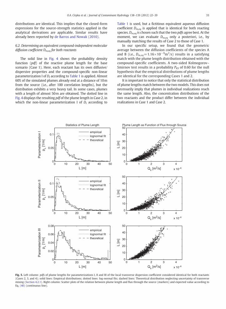
Fig. 5. Left column: pdfs of plume lengths for parameterizations I, II and III of the l(Cases 2, 3, and 4); solid lines: Empirical distributions; dotted lines: log-normal fitmixing (Section 4.2.1). Right column: Scatter plots of the relation between plume leEq. (40) (continuous line).

Table 1 is used, but a fictitious equivalent aqueous diffusioncoefficient Dm,eq is applied that is identical for both reactingspecies.Dm,eq is chosen such that the two pdfs agree best. At themoment, we can evaluate Dm,eq only a posteriori, i.e., bymanually matching the results of Case 2 to those of Case 1.

In our specific setup, we found that the geometricaverage between the diffusion coefficients of the species Aand B (i.e., Dm,eq=1.16×10−9m2/s) results in a satisfyingmatch with the plume length distribution obtained with thecompound-specific coefficients. A two-sided Kolmogorov–Smirnov test results in a probability PKS of 0.60 for the nullhypothesis that the empirical distributions of plume lengthsare identical for the corresponding Cases 1 and 2.

It is important to notice that only the statistical distributionof plume lengthsmatch between the twomodels. This does notnecessarily imply that plumes in individual realizations reachthe same length. Also, the concentration distributions of thetwo reactants and the product differ between the individualrealizations in Case 1 and Case 2.

0 1 2 3 4

x 10−6

0

10

20

30

40

50

Qs [m2/s]

0 1 2 3 4

x 10−6Qs [m2/s]

0 1 2 3 4

x 10−6Qs [m2/s]

L [m

]

0

10

20

30

40

50

L [m

]

0

10

20

30

40

50

L [m

]

Plume Length as Function of Flux through Source

ocal transverse dispersion coefficient considered identical for both reactantss; dashed lines: Theoretical distribution neglecting uncertainty of transversength and flux through the source (markers) and expected value according to

34 O.A. Cirpka et al. / Journal of Contaminant Hydrology 138–139 (2012) 22–39

6.3. Statistical distributions of plume length for identical localtransverse dispersion coefficients and uncertain source strength

Fig. 5 shows the results from all scenarios that useequivalent aqueous diffusion coefficients (Cases 2, 3 and 4),but with different descriptions of local mechanical dispersionDt (parameterizations I, II, and III in Table 1). The left columnof subplots shows the different pdfs of the computed plumelengths. The empirical distributions, shown as histograms, arecompared to log-normal fits (dotted lines) and to the theoreticaldistributions (dashed lines) according to Section 4.2.1. Theseanalytical solutions neglect the uncertainty of transversemixing.The plume length in a homogeneous medium with a constantconductivity value set to the effective value of the heterogeneouscases (K=Kg)would be 27.4m,which is considerably larger thanthemean plume length in the tested heterogeneous cases due tothe mixing enhancement by flow focusing.

The right column of subplots illustrates the relationshipbetween the volumetric flux through the contamination sourceQs and the computed plume length L. The average behavior iswell captured by a quadratic relationship between L and Qs

(compare Eq. (40)), when inserting the equivalent transversedispersion coefficients Dt

eq according to Eq. (36) (Cirpka et al.,2011b). Despite a good match in the average behavior, thenumerical results show a considerable scattering around thetrend line, due to the uncertainty in mixing. The degree ofscattering about the mean behavior is the highest for param-eterization II of local transverse dispersion (linear dependenceon velocity, local transverse dispersivity scales with

ffiffiffiffiK

p). For

parameterization I, the scatter is somewhat smaller, reflectingthe less-than-linear dependence of Dt on v, whereas usingScheidegger's (1961) parameterization with constant αt resultsin the smallest scatter.

Table 4 lists the computed equivalent transverse dispersioncoefficients Dt

eq according to Eq. (36) for all test cases. AssumingScheidegger's (1961) parameterization of local transversedispersion with constant dispersivity αt (parameterization III,Case 4) results in the smallest value ofDt

eq and thus in the largestmean plume length. This is so, even though the local transversedispersion coefficients fluctuate about the same mean. Thedifference to parameterizations I (Case 2) and II (Case 3) issignificant, emphasizing the importance of choosing an adequate

Table 4Metrics of the numerical test cases. Dt-model refers to the local transverse dispersiondispersion coefficient of Eq. (36). Case 1 is compared to Case 2 as “theoretical model”the semi-analytical approaches of Section 4.2.

Statistical metrics of plume lengths

Empirical Log-normal fi

Case Dt-model Dteq [m2/s] Mean [m] Std.dev. [m] Mean [m]

1 I n.a. 9.39 7.75 9.632 I 4.63×10−9 9.36 7.72 9.693 II 5.23×10−9 8.66 7.30 9.03

4 III 3.00×10−9 12.4 9.25 13.9

Empirical Normal fit

5 I 4.63×10−9 7.84 2.32 7.846 III 3.00×10−9 11.5 2.56 11.5

parameterization for the local transverse dispersion coefficient inreactive transport simulations.

Table 4 also includes statistical metrics of the plume-lengthdistributions. The empirical distributions consistently showless variation than the fitted and predicted ones, whichmay beattributed to missing values beyond L=50m in the numericalsetup. The resulting coefficients of variation are about unity,implying high uncertainty in the prediction of plume lengths.

6.4. Comparison of simplifying assumptions in the analyticalderivations

Fig. 5 also includes the analytical expressions (“theoret-ical”) based on the simplest analytical approach (Eq. 40 fromSection 4.2.1) as dashed lines, for direct comparison with thecorresponding numerical Cases 2, 3 and 4. In that simpleapproach, the mean enhancement of transverse mixing isaccounted for, but its uncertainty is neglected, resulting in alog-normal distribution of L mapped from the distribution ofthe source strength Qs. A visual inspection implies a decentapproximation of the statistical plume-length distributionusing this simple analytical approach. Table 4 includes thecorresponding probabilities of Kolmogorov–Smirnov tests onthe null hypothesis that the empirical and predicteddistributions are identical. Based on a sample size of n=1000 and a confidence level of 5%, this hypothesis must berejected for Cases 2 and 3 (in spite of the decent visual fit),whereas it is accepted for Case 4.

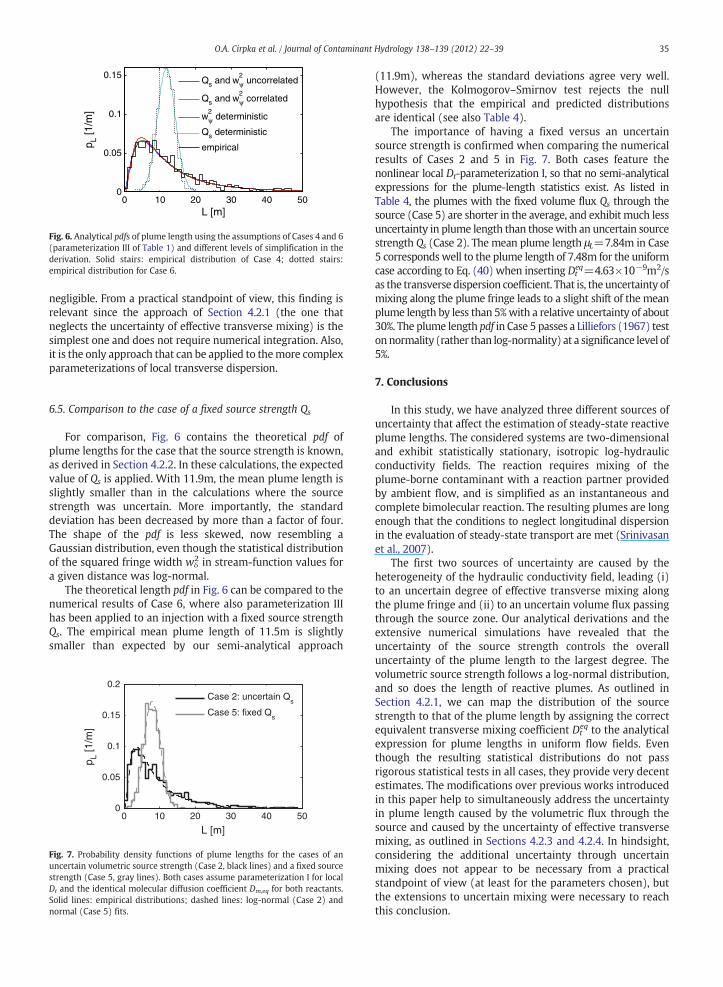
Fig. 6 compares all semi-analytical expressions for theplume-length statistics derived in Section 4.2. The deriva-tions are based on the local Dt-parameterization III, and weapply the same parameters as in Case 4. As reference, Fig. 6also contains the empirical distributions from Cases 4 and 6,and Table 4 lists the corresponding statistical metrics.Visually, the semi-analytical approaches of Sections 4.2.1,4.2.3, and 4.2.4 appear almost identical. As revealed in Table 4,the simplest model, in which the uncertainty of mixing isneglected, leads to a slightly larger mean plume length.However, all three approaches pass the Kolmogorov–Smirnovtest. This implies that the uncertainty of the volumetric sourcestrength Qs is so overwhelming, that considering the concur-rent uncertainty of effective transverse mixing becomes

parameterizations listed in Table 1, Dteq to the upscaled equivalent transverse

; Case 5 is compared to a normal distribution; all other cases are compared to

t Theoretical Goodness of theory

Std.dev. [m] Mean [m] Std.dev. [m] Theoretical model PKS

9.39 n.a. n.a. Case 2 0.609.74 8.94 9.13 Section 4.2.1 0.009.11 7.92 8.09 Section 4.2.1 0.00

13.7 13.5 Section 4.2.1 0.2513.8 13.3 11.4 Section 4.2.3 0.25

13.3 11.3 Section 4.2.4 0.39

Plillie

2.32 n.a. n.a. Normal distr. 0.342.56 11.9 2.53 Section 4.2.2 0.00

L [m]

p L [1

/m]

0 10 20 30 40 500

0.05

0.1

0.15 Qs and w2ψ uncorrelated

Qs and w2ψ correlated

w2ψ deterministic

Qs deterministic

empirical

Fig. 6. Analytical pdfs of plume length using the assumptions of Cases 4 and 6(parameterization III of Table 1) and different levels of simplification in thederivation. Solid stairs: empirical distribution of Case 4; dotted stairs:empirical distribution for Case 6.

35O.A. Cirpka et al. / Journal of Contaminant Hydrology 138–139 (2012) 22–39

negligible. From a practical standpoint of view, this finding isrelevant since the approach of Section 4.2.1 (the one thatneglects the uncertainty of effective transverse mixing) is thesimplest one and does not require numerical integration. Also,it is the only approach that can be applied to themore complexparameterizations of local transverse dispersion.

6.5. Comparison to the case of a fixed source strength Qs

For comparison, Fig. 6 contains the theoretical pdf ofplume lengths for the case that the source strength is known,as derived in Section 4.2.2. In these calculations, the expectedvalue of Qs is applied. With 11.9m, the mean plume length isslightly smaller than in the calculations where the sourcestrength was uncertain. More importantly, the standarddeviation has been decreased by more than a factor of four.The shape of the pdf is less skewed, now resembling aGaussian distribution, even though the statistical distributionof the squared fringe width wδ

2 in stream-function values fora given distance was log-normal.

The theoretical length pdf in Fig. 6 can be compared to thenumerical results of Case 6, where also parameterization IIIhas been applied to an injection with a fixed source strengthQs. The empirical mean plume length of 11.5m is slightlysmaller than expected by our semi-analytical approach

L [m]

p L [1

/m]

0 10 20 30 40 500

0.05

0.1

0.15

0.2Case 2: uncertain Q

s

Case 5: fixed Qs

Fig. 7. Probability density functions of plume lengths for the cases of anuncertain volumetric source strength (Case 2, black lines) and a fixed sourcestrength (Case 5, gray lines). Both cases assume parameterization I for localDt and the identical molecular diffusion coefficient Dm,eq for both reactants.Solid lines: empirical distributions; dashed lines: log-normal (Case 2) andnormal (Case 5) fits.

(11.9m), whereas the standard deviations agree very well.However, the Kolmogorov–Smirnov test rejects the nullhypothesis that the empirical and predicted distributionsare identical (see also Table 4).

The importance of having a fixed versus an uncertainsource strength is confirmed when comparing the numericalresults of Cases 2 and 5 in Fig. 7. Both cases feature thenonlinear local Dt-parameterization I, so that no semi-analyticalexpressions for the plume-length statistics exist. As listed inTable 4, the plumes with the fixed volume flux Qs through thesource (Case 5) are shorter in the average, and exhibit much lessuncertainty in plume length than thosewith an uncertain sourcestrength Qs (Case 2). The mean plume length μL=7.84m in Case5 correspondswell to the plume length of 7.48m for the uniformcase according to Eq. (40) when inserting Dt

eq=4.63×10−9m2/sas the transverse dispersion coefficient. That is, the uncertainty ofmixing along the plume fringe leads to a slight shift of the meanplume length by less than 5%with a relative uncertainty of about30%. The plume length pdf in Case 5 passes a Lilliefors (1967) testonnormality (rather than log-normality) at a significance level of5%.

7. Conclusions

In this study, we have analyzed three different sources ofuncertainty that affect the estimation of steady-state reactiveplume lengths. The considered systems are two-dimensionaland exhibit statistically stationary, isotropic log-hydraulicconductivity fields. The reaction requires mixing of theplume-borne contaminant with a reaction partner providedby ambient flow, and is simplified as an instantaneous andcomplete bimolecular reaction. The resulting plumes are longenough that the conditions to neglect longitudinal dispersionin the evaluation of steady-state transport are met (Srinivasanet al., 2007).

The first two sources of uncertainty are caused by theheterogeneity of the hydraulic conductivity field, leading (i)to an uncertain degree of effective transverse mixing alongthe plume fringe and (ii) to an uncertain volume flux passingthrough the source zone. Our analytical derivations and theextensive numerical simulations have revealed that theuncertainty of the source strength controls the overalluncertainty of the plume length to the largest degree. Thevolumetric source strength follows a log-normal distribution,and so does the length of reactive plumes. As outlined inSection 4.2.1, we can map the distribution of the sourcestrength to that of the plume length by assigning the correctequivalent transverse mixing coefficient Dt

eq to the analyticalexpression for plume lengths in uniform flow fields. Eventhough the resulting statistical distributions do not passrigorous statistical tests in all cases, they provide very decentestimates. The modifications over previous works introducedin this paper help to simultaneously address the uncertaintyin plume length caused by the volumetric flux through thesource and caused by the uncertainty of effective transversemixing, as outlined in Sections 4.2.3 and 4.2.4. In hindsight,considering the additional uncertainty through uncertainmixing does not appear to be necessary from a practicalstandpoint of view (at least for the parameters chosen), butthe extensions to uncertain mixing were necessary to reachthis conclusion.

36 O.A. Cirpka et al. / Journal of Contaminant Hydrology 138–139 (2012) 22–39

In the chosen test case, the geometric width of the plumewas 1.5 times the integral scale of the heterogeneouslog-conductivity field. For wider sources, the relative uncer-tainty of the volumetric source strength Qs would decrease(leading order: σQs

2∝1/ws2), as shown by de Barros and Nowak

(2010). However, wider sources also imply considerably longerplumes (leading order: L∝w2) which leads to a reduction ofrelative uncertainty in cumulative transverse mixing (leadingorder: σwδ(x)

22∝1/x).We thus expect that the higher importance

of the source-strength uncertainty in comparison to that ofeffective transverse mixing will also prevail for wider plumes.

Increasing the degree of heterogeneity, σY2, will increase the

uncertainty of both cumulative mixing and source strength, sothat the relative importance of these sources of uncertainty isexpected to be similar. However, at high values of σY

2 allfirst-order expressions become invalid. Changing the stoichiom-etry of the reaction, or the concentrations of the end-membersolutions, will only affect the mean plume length and thus theuncertainty of cumulativemixing,whereas theuncertainty of thesource strength would remain untouched. That is, a small inflowconcentration of the plume-borne compoundA in comparison tothe ambient concentration of compound B could make theuncertainty of cumulative mixing somewhat more important incomparison to the uncertainty of the source strength.

The third source of uncertainty considered in this study isconceptual in nature and deals with the parameterization usedfor local transverse dispersion.Whilemany traditional studies ondispersion in heterogeneous porous media (e.g., Dentz et al.,2000; Fiori and Dagan, 2000) assume a uniform local dispersiontensor, we have tested models in which Dt depends on the localvelocity or, in some cases, explicitly on the value of the hydraulicconductivity. As already analyzed by Cirpka et al. (2011b), themean enhancement of transverse mixing by hydraulic hetero-geneity depends on the chosen parameterization ofDt. The effectis the largest in the case where Dt is assumed to depend linearlyon velocity and the transverse dispersivity αt is assumed to scalewith

ffiffiffiffiK

p(parameterization II). The effect is the smallest when a

uniform and K-independent value of αt is assumed (parameter-ization III, (Scheidegger, 1961)), whereas the nonlinear param-eterization of Chiogna et al. (2010) leads to an intermediateenhancement of transverse mixing. The different meanmixing-enhancement factors directly lead to different meanplume lengths, whereas the coefficients of variation are hardlyaffected and have been found to be about unity in all our testcases.

Applying the nonlinear parameterization of Chiogna et al.(2010) for local transverse dispersion implies a significantcompound-dependence of transverse dispersion at all veloci-ties. This puts all approaches of mixing-controlled reactivetransport, which are based on the concept of a conservativespecies mixing ratio, into question. In fact, such approachesassume identical dispersion of all reactants. For that reason, wehave also simulated the case inwhich the two reactants exhibitdifferent transverse mixing behavior. In our application, wereplaced the two molecular diffusion coefficients of thereacting species with their geometric mean. Then, wesubstituted the geometric mean into expressions based onthe compound-independent mixing ratio and obtained almostidentical plume-length statistics. At our current state ofknowledge, however, we cannot state whether the geometricmean is applicable in all situations.

Our study has been restricted to two-dimensional domains.Additional effects of heterogeneity on effective transversemixing in three spatial dimensions need to be analyzedindependently. Also, all considerations presented are validunder the assumption that the reactions are controlled bymixing of the reactants. For reactive transport problems inwhich the reaction kinetics can be identified as the rate limitingstep to the overall degradation, also the uncertainty related tothe (bio)chemical reactions should be included in the analysis.

Acknowledgments

This study was supported by Deutsche Forschungsge-meinschaft (DFG) via the Cluster of Excellence in SimulationTechnology (EXC 310/1) at the University of Stuttgart, by theSpanish Ministry of Science via the “Juan de la Cierva”program, by the Marie Curie International Outgoing Fellow-ship (DILREACT project) within the 7th European Communi-ty Framework Programme, and by the EU 7th FrameworkProgramme Collaborative Research Project CLIMB (ClimateInduced Changes on the Hydrology of Mediterranean Basins)grant 244151. The authors would like to acknowledge thecomments and suggestions made by Marco Dentz and AlbertValocchi.

Appendix A. Variance of Qs according to de Barros andNowak (2010)

de Barros and Nowak (2010) approximated the varianceof the cumulative specific discharge Qs passing through a lineperpendicular to the direction of flow with length ws for thecase of uniform-in-the-mean flow and an exponential isotropiccovariance function of log hydraulic conductivity to the firstorder as:

σ2Qs≈K2

g J2σ2

Yðγ−12þ exp −ws

λ

� �−3λ2

w2sþ exp −ws

λ

� �3þ 3 wsλ þ w2

s

λ2

ws=λð Þ2þE1

ws

λ

� �þ ln

ws

λ

� �ÞðA:1Þ

in which γ≈0.577216 is the Euler–Mascheroni constant andE1(x)=∫x

∞exp(−t)/tdt is the exponential integral function.

Appendix B. Variance of wδ2(x1) according to Cirpka et al.

(2011b)

For the case of the linear Scheidegger model for trans-verse dispersion with constant dispersivity αt,uniform-in-the-mean flow in direction x1, and an exponentialisotropic covariance function of log hydraulic conductivity,Cirpka et al. (2011b) give estimate the coefficient of variationof wδ

2(x1) to the first order as:

CVw2δ x1ð Þ≈

σYλ

x1 Dp þαt

θJKg

� ��…

…�ffiffiffiffiffiffiffiffiffiffiffiffiffiffiffiffiffiffiffiffiffiffiffiffiffiffiffiffiffiffiffiffiffiffiffiffiffiffiffiffiffiffiffiffiffiffiffiffiffiffiffiffiffiffiffiffiffiffiffiffiffiffiffiffiffiffiffiffiffiffiffiffiffiffiffiffiffiffiffiffiffiffiffiffiffiffiffiffiffiffiffiffiffiffiffiffiffiffiffiffiffiffiffiffiffiffiffiffiffiffiffiffiffiffiffiffiffiffiffiffiffiffiffiffiffiffiffiffiffiffiffiffiffiffiffiffiffiffiffiffiffiffiffiffiffiffiffiffiffiffiffiffiffiffiffi3K2

g J2 α

2t

θ2A1 x1ð Þ þ 4 Dp þ

αt

θJKg

� �αt

θJKgA2 x1ð Þ þ 2 Dp þ

αt

θJKg

� �2A3 x1ð Þs

ðB:1Þ

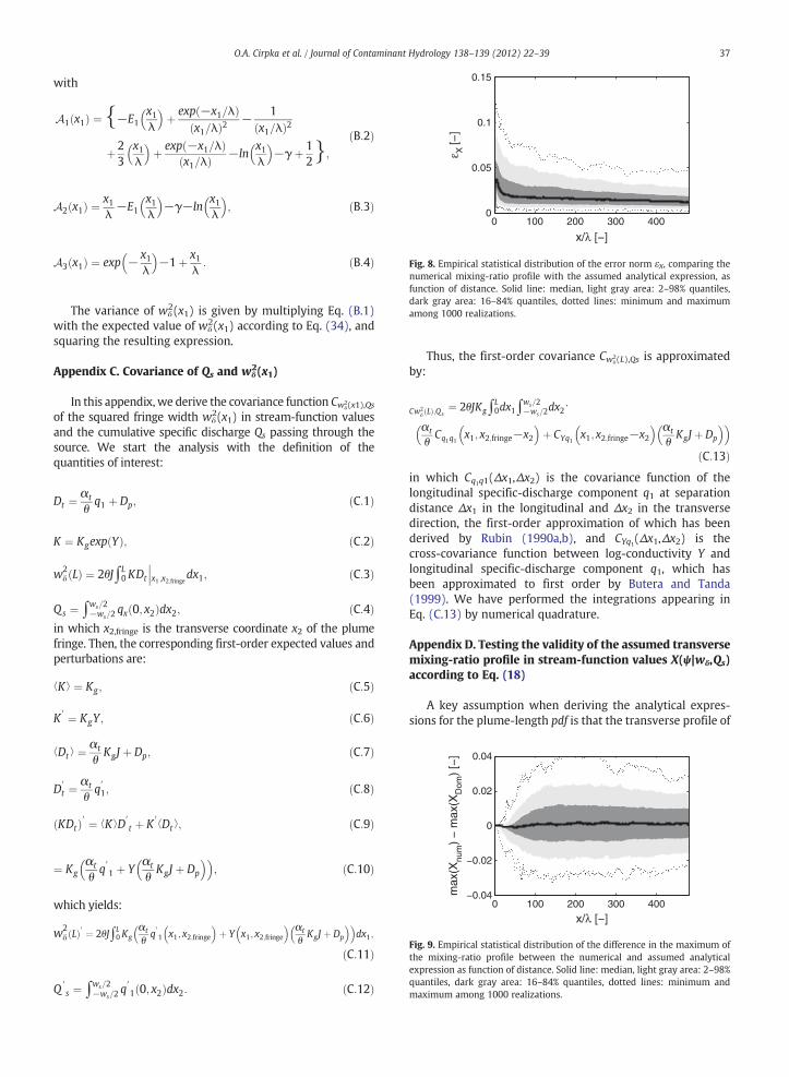
x/λ [−]

ε X [−

]

0 100 200 300 4000

0.05

0.1

0.15

Fig. 8. Empirical statistical distribution of the error norm εX, comparing thenumerical mixing-ratio profile with the assumed analytical expression, asfunction of distance. Solid line: median, light gray area: 2–98% quantiles,dark gray area: 16–84% quantiles, dotted lines: minimum and maximumamong 1000 realizations.

x/λ [−]

max

(Xnu

m)

− m

ax(X

Dom

) [−

]

0 100 200 300 400−0.04

−0.02

0

0.02

0.04

Fig. 9. Empirical statistical distribution of the difference in the maximum ofthe mixing-ratio profile between the numerical and assumed analyticalexpression as function of distance. Solid line: median, light gray area: 2–98%quantiles, dark gray area: 16–84% quantiles, dotted lines: minimum andmaximum among 1000 realizations.

37O.A. Cirpka et al. / Journal of Contaminant Hydrology 138–139 (2012) 22–39

with

A1 x1ð Þ ¼ f−E1x1λ

� �þ exp −x1=λð Þ

x1=λð Þ2 − 1x1=λð Þ2

þ23

x1λ

� �þ exp −x1=λð Þ

x1=λð Þ −lnx1λ

� �−γ þ 1

2g;

ðB:2Þ

A2 x1ð Þ ¼ x1λ−E1

x1λ

� �−γ−ln

x1λ

� �; ðB:3Þ

A3 x1ð Þ ¼ exp − x1λ

� �−1þ x1

λ: ðB:4Þ

The variance of wδ2(x1) is given by multiplying Eq. (B.1)

with the expected value of wδ2(x1) according to Eq. (34), and

squaring the resulting expression.

Appendix C. Covariance of Qs and wδ2(x1)

In this appendix,we derive the covariance function Cwδ2(x1),Qs

of the squared fringe width wδ2(x1) in stream-function values

and the cumulative specific discharge Qs passing through thesource. We start the analysis with the definition of thequantities of interest:

Dt ¼αt

θq1 þ Dp; ðC:1Þ

K ¼ Kgexp Yð Þ; ðC:2Þ

w2δ Lð Þ ¼ 2θJ∫L

0KDt x1 ;x2;fringedx1;

ðC:3Þ

Qs ¼ ∫ws=2−ws=2

qx 0; x2ð Þdx2; ðC:4Þin which x2,fringe is the transverse coordinate x2 of the plumefringe. Then, the corresponding first-order expected values andperturbations are:

⟨K⟩ ¼ Kg ; ðC:5Þ

K ′ ¼ KgY ; ðC:6Þ

⟨Dt⟩ ¼αt

θKgJ þ Dp; ðC:7Þ

D′t ¼

αt

θq′1; ðC:8Þ

ðKDtÞ′ ¼ ⟨K⟩D′t þ K ′

⟨Dt⟩; ðC:9Þ

¼ Kgαt

θq′1 þ Y

αt

θKgJ þ Dp

� �� �; ðC:10Þ

which yields:

w2δ ðLÞ′ ¼ 2θJ∫L

0 Kgαt

θq′1 x1; x2;fringe� �

þ Y x1; x2;fringe� � αt

θKgJ þ Dp

� �� �dx1;

ðC:11Þ

Q ′s ¼ ∫ws=2

−ws=2q′1 0; x2ð Þdx2: ðC:12Þ

Thus, the first-order covariance Cwδ2(L),Qs is approximated

by:

Cw2δ Lð Þ;Qs

¼ 2θJKg∫L0dx1∫

ws=2−ws=2

dx2⋅αt

θCq1q1

x1; x2;fringe−x2� �

þ CYq1x1; x2;fringe−x2� � αt

θKgJ þ Dp

� �� �ðC:13Þ

in which Cq1q1(Δx1,Δx2) is the covariance function of thelongitudinal specific-discharge component q1 at separationdistance Δx1 in the longitudinal and Δx2 in the transversedirection, the first-order approximation of which has beenderived by Rubin (1990a,b), and CYq1(Δx1,Δx2) is thecross-covariance function between log-conductivity Y andlongitudinal specific-discharge component q1, which hasbeen approximated to first order by Butera and Tanda(1999). We have performed the integrations appearing inEq. (C.13) by numerical quadrature.

Appendix D. Testing the validity of the assumed transversemixing-ratio profile in stream-function values X(ψ|wδ,Qs)according to Eq. (18)

A key assumption when deriving the analytical expres-sions for the plume-length pdf is that the transverse profile of

0.9

0.95

1

1.05

1.1

w2 δ

,num

w2 δ

,theo

r

[−]

x/λ [−]

0 100 200 300 400 5000

0.25

0.5

0.75

1

CV

w [

−]

2 δ

Fig. 10. Comparison of statisticalmetrics of the fringewidth in stream-functioncoordinates between the analytical expressions of Cirpka et al. (2011b) and thevalues evaluated from the numerical extended-source calculations. Solid lineand left axis: ratio of mean squared numerical fringe width in stream‐functioncoordinates to the analytical expression of Cirpka et al. (2011a,b); dashed lineand right axis: coefficient of variation of the squared fringe width in stream‐

function coordinates; black lines: numerical results from 1000 realizations;gray lines: expressions of Cirpka et al. (2011a,b).

38 O.A. Cirpka et al. / Journal of Contaminant Hydrology 138–139 (2012) 22–39

the mixing ratio in stream-function coordinates X(ψ) followsthe functional shape of (Domenico and Palciauskas, 1982),Eq. (18), even though the underlying hydraulic-conductivityis heterogeneous. We test this by analyzing the numericalmixing-ratio profiles computed for Case 6 (fixed sourcestrength, linear transverse dispersion coefficients with uni-form dispersivity). First, we evaluate the center position ψc

and the squared fringe width wδ2 in stream-function values of

the transverse profiles for all distances in all realizationsaccording to Eqs. (19 and 20). Then, we substitute them intoEq. (18) to obtain a theoretical profile Xtheor(ψ|wδ

2(x)), whichwe compare to the numerical profile using the followingerror norm:

εX x1ð Þ ¼ffiffiffiffiffiffiffiffiffiffiffiffiffiffiffiffiffiffiffiffiffiffiffiffiffiffiffiffiffiffiffiffiffiffiffiffiffiffiffiffiffiffiffiffiffiffiffiffiffiffiffiffiffiffiffiffiffiffiffiffiffiffiffiffiffiffiffiffiffiffiffiffiffiffiffiffiffi∫þ∞−∞ Xnum x1;ψð Þ−Xtheor ψð jw2

δ xð Þ� �Þ2qdψ

QsD:1

Fig. 8 shows the empirical statistical distribution of εX(x1)as function of distance x1. The 2nd and 98th percentileswould denote the range of ±two standard deviations aboutthe mean, whereas the 16th and 84th percentiles areequivalent to the range of ±one standard deviation aboutthe mean, both if the distribution was Gaussian. At shorttravel distances (x1b20λ), the numerical and theoreticalprofiles tend to deviate somewhat more significantly,typically at the plume fringe. This deviation does practicallynot affect the ability to predict the maximum value of theprofile. Fig. 9 shows the empirical statistical distribution ofthe difference in the maximum of the mixing-ratio profilesbetween the numerical and assumed analytical expressionsaccording to Eq. (21) as function of distance. 95% are coveredin a range of ±0.02. We conclude that the assumeddependence of max(X(ψ|Qs,wδ

2(x1))) on Qs and wδ2(x1) is

applicable.

Appendix E. Testing the validity of the analytical fringe-width statistics of Cirpka et al. (2011b) to the extendedline-source problem

A second assumption when deriving the plume-length pdfis that the analytical results of the squared fringe-width

statistics derived by Cirpka et al. (2011b) for a point injectionalso apply to the line source considered here. For this purpose,we consider the same Monte Carlo simulations as in AppendixD and compare the mean and coefficient of variation of theempirical values of wδ

2(x1), as computed by Eq. (20) to theanalytical results of Eqs. (34) and (B.1). Fig. 10 shows thecorresponding profiles. There is a slight underestimation of themean by the theoretical model, and a slight overestimation ofthe coefficient of variation. The empirical statistical distributionof wδ

2 resembles a log-normal profile (results not shown).

References

Bauer, R.D., Rolle, M., Bauer, S., Eberhardt, C., Grathwohl, P., Kolditz, O.,Meckenstock, R.U., Griebler, C., 2009a. Enhanced biodegradation byhydraulic heterogeneities in petroleum hydrocarbon plumes. Journal ofContaminant Hydrology 105, 56–68.

Bauer, R.D., Rolle, M., Kuerzinger, P., Grathwohl, P., Meckenstock, R.U.,Griebler, C., 2009b. Two-dimensional flow-through microcosms —

versatile test systems to study biodegradation processes in porousaquifers. Journal of Hydrology 369, 284–295.

Bear, J., 1972. Dynamics of Fluids in Porous Media. American Elsevier, NewYork.

Butera, I., Tanda, M.G., 1999. Solute transport analysis through heteroge-neous media in nonuniform in the average flow by a stochasticapproach. Transport Porous Media 36, 255–291.

Chiogna, G., Eberhardt, C., Grathwohl, P., Cirpka, O.A., Rolle, M., 2010.Evidence of compound dependent hydrodynamic and (hydro)mechan-ical transverse dispersion by multi-tracer laboratory experiments.Environmental Science & Technology 44, 688–693.

Chiogna, C., Cirpka, O.A., Grathwohl, P., Rolle, M., 2011a. Relevance of localcompound-specific transverse dispersion for conservative and reactivemixing in heterogeneous porous media. Water Resources Research 47,W07540.

Chiogna, G., Cirpka, O.A., Grathwohl, P., Rolle, M., 2011b. Transverse mixingof conservative and reactive tracers in porous media: quantificationthrough the concepts of flux-related and critical dilution indices. WaterResources Research 47, W02505.

Cirpka, O.A., Valocchi, A.J., 2007. Two-dimensional concentration distribu-tion for mixing-controlled bioreactive transport in steady state.Advances in Water Resources 30, 1668–1679.

Cirpka, O.A., Frind, E.O., Helmig, R., 1999a. Numerical simulation ofbiodegradation controlled by transverse mixing. Journal of ContaminantHydrology 40, 159–182.

Cirpka, O.A., Frind, E.O., Helmig, R., 1999b. Streamline-oriented grid-generation for transport modelling in two-dimensional domainsincluding wells. Advances in Water Resources 22, 697–710.

Cirpka, O.A., Helmig, R., Frind, E.O., 1999c. Numerical methods for reactivetransport on rectangular and streamline-oriented grids. Advances inWater Resources 22, 711–728.

Cirpka, O.A., Windfuhr, C., Bisch, G., Granzow, S., Scholz-Muramatsu, H.,Kobus, H., 1999d. Microbial reductive dechlorination in large-scalesandbox model. Journal of Environmental and Engineering, ASCE 125,861–870.

Cirpka, O.A., Olsson, Å., Ju, Q., Rahman, M.A., Grathwohl, P., 2006.Determination of transverse dispersion coefficients from reactiveplume lengths. Ground Water 44, 212–221.

Cirpka, O.A., de Barros, F.P.J., Chiogna, G., Nowak, W., 2011a. Probabilitydensity function of steady-state concentration in two-dimensionalheterogeneous porous media. Water Resources Research 47, W11523.

Cirpka, O.A., de Barros, F.P.J., Chiogna, G., Rolle, M., Nowak, W., 2011b.Stochastic flux-related analysis of transverse mixing in two-dimensionalheterogeneous porous media. Water Resources Research 47, W06515.

Dagan, G., 1984. Solute transport in heterogeneous porous formations.Journal of Fluid Mechanics 145, 151–177.

Davis, G.B., Barber, C., Power, T.R., Thierrin, J., Patterson, B.M., Rayner, J.L.,Wu, Q., 1999. The variability and intrinsic remediation of a btex plume inanaerobic sulphate-rich groundwater. Journal of Contaminant Hydrolo-gy 36, 265–290.

de Barros, F.P.J., Nowak, W., 2010. On the link between contaminant sourcerelease conditions and plume prediction uncertainty. Journal ofContaminant Hydrology 116, 24–34.

De Simoni, M., Carrera, J., Sanchez-Vila, X., Guadagnini, A., 2005. A procedurefor the solution of multicomponent reactive transport problems. WaterResources Research 41, W11410.

39O.A. Cirpka et al. / Journal of Contaminant Hydrology 138–139 (2012) 22–39

De Simoni, M., Sanchez-Vila, X., Carrera, J., Saaltink, M.W., 2007. A mixingratios-based formulation for multicomponent reactive transport. WaterResources Research 43, W07419.

Delgado, J.M.P.Q., 2006. A critical review of dispersion in packed beds. Heatand Mass Transfer 42 (4), 279–310. http://dx.doi.org/10.1007/s00231-005-0019-0.

Dentz, M., Kinzelbach, H., Attinger, S., Kinzelbach, W., 2000. Temporalbehavior of a solute cloud in a heterogeneous porous medium 1. Point-like injection. Water Resources Research 36, 3591–3604.

Dietrich, C., Newsam, G., 1993. A fast and exact method for multidimensionalGaussian stochastic simulations. Water Resources Research 29, 2861–2869.

Domenico, P., 1987. An analytical model for multidimensional transport of adecaying contaminant species. Journal of Hydrology 91, 49–58.

Domenico, P.A., Palciauskas, V.V., 1982. Alternative boundaries in solid wastemanagement. Ground Water 20, 303–311.

Domenico, P., Robbins, G., 1985. A new method of contaminant plumeanalysis. Ground Water 23, 476–485.

Fiori, A., Dagan, G., 2000. Concentration fluctuations in aquifer transport: arigorous first-order solution and applications. Journal of ContaminantHydrology 45, 139–163.

Fraser, M., Barker, J., Butler, B., Blaine, F., Joseph, S., Cooke, C., 2008. Naturalattenuation of a plume from an emplaced coal tar creosote source over14years. Journal of Contaminant Hydrology 100, 101–115.

Freeze, R.A., 1975. A stochastic–conceptual analysis of one-dimensionalgroundwater flow in nonuniform homogeneous media. Water ResourcesResearch 11, 725–741.

Gelhar, L.W., Axness, C.L., 1983. Three-dimensional stochastic analysis ofmacrodispersion in aquifers. Water Resources Research 19, 161–180.

Ham, P.A.S., Schotting, R.J., Prommer, H., Davis, G.B., 2004. Effects ofhydrodynamic dispersion on plume lengths for instantaneous bimolec-ular reactions. Advances in Water Resources 27, 803–813.

Hazen, A., 1892. Some physical properties of sands and gravels with specialreference to their use in filtration. Ann. Rep. State Board of Health Mass.24, pp. 541–556.

Huang, W.E., Oswald, S.E., Lerner, D.N., Smith, C.C., Zheng, C., 2003. Dissolvedoxygen imaging in a porous medium to investigate biodegradation in aplume with limited electron acceptor supply. Environmental Science &Technology 37, 1905–1911.

King, M.W.G., Barker, J.F., 1999. Migration and natural fate of a coal tarcreosote plume 1. Overview and plume development. Journal ofContaminant Hydrology 39, 249–279.

Le Borgne, T., Dentz, M., Bolster, D., Carrera, J., de Dreuzy, J.R., Davy, P., 2010.Non-Fickian mixing: temporal evolution of the scalar dissipation rate inheterogeneous porous media. Advances in Water Resources 33,1468–1475.

Leube, P., Geiges, A., Nowak, W., 2012. Bayesian assessment of the expecteddata impact on prediction confidence in optimal sampling design. WaterResources Research 48, W02501.

Liedl, R., Valocchi, A.J., Dietrich, P., Grathwohl, P., 2005. Finiteness of steadystate plumes. Water Resources Research 31, W12501.

Liedl, R., Yadav, P.K., Dietrich, P., 2011. Length of 3-d mixing-controlledplumes for a fully penetrating contaminant source with finite width.Water Resources Research 47, W08602.

Lilliefors, H.W., 1967. On the Kolmogorov–Smirnov test for normality withmean and variance unknown. Journal of the American StatisticalAssociation 62, 399–402.

Mace, R.E., Fisher, R.S., Welch, D., Parra, S., 1997. Extent, mass, and durationof hydrocarbon plumes from leaking petroleum storage tank sites inTexas. Geologic Circular, 97-1. Bureau of Economic Geology, Universityof Texas at Austin.

Maier, U., Grathwohl, P., 2006. Numerical experiments and field results onthe size of steady state plumes. Journal of Contaminant Hydrology 85,33–52.

Nowak, W., Cirpka, O.A., 2006. Geostatistical inference of hydraulicconductivity and dispersion coefficients from hydraulic heads and tracerdata. Water Resources Research 42, W08416. http://dx.doi.org/10.1029/2005WR004832.

Nowak, W., Schwede, R.L., Cirpka, O.A., Neuweiler, I., 2008. Probabilitydensity functions of hydraulic head and velocity in three-dimensionalheterogeneous porous media. Water Resources Research 44, W08452.

Nowak, W., de Barros, F.P.J., Rubin, Y., 2010. Bayesian geostatistical design:optimal site investigation when the geostatistical model is uncertain.Water Resources Research 46, W03535.

Olsson, Å., Grathwohl, P., 2007. Transverse dispersion of non-reactive tracersin porous media: a new nonlinear relationship to predict dispersioncoefficients. Journal of Contaminant Hydrology 92, 149–161.

Prommer, H., Tuxen, N., Bjerg, P.L., 2006. Fringe-controlled naturalattenuation of phenoxy acids in a landfill plume: integration of field-scale processes by reactive transport modeling. Environmental Science &Technology 40, 4732–4738.

Prommer, H., Anneser, B., Rolle, M., Einsiedl, F., Griebler, C., 2009.Biogeochemical and isotopic gradients in a BTEX/PAH contaminantplume: model-based interpretation of a high-resolution field data set.Environmental Science & Technology 43, 8206–8212.

Rahman, M.A., Jose, S.C., Nowak, W., Cirpka, O.A., 2005. Experiments onvertical transverse mixing in a large-scale heterogeneous model aquifer.Journal of Contaminant Hydrology 80, 130–148.

Rolle, M., Eberhardt, C., Chiogna, G., Cirpka, O.A., Grathwohl, P., 2009.Enhancement of dilution and transverse reactive mixing in porousmedia: experiments and model-based interpretation. Journal of Con-taminant Hydrology 110, 130–142.

Rubin, Y., 1990a. Correction to “stochastic modeling of macrodispersion inheterogeneous porous media”. Water Resources Research 26, 2631.

Rubin, Y., 1990b. Stochastic modeling of macrodispersion in heterogeneousporous media. Water Resources Research 26, 133–141.

Rubin, Y., 2003. Applied Stochastic Hydrogeology. Oxford University Press,Oxford.

Scheidegger, A.E., 1961. General theory of dispersion in porous media.Journal of Geophysical Research 66, 3273–3278.

Srinivasan, V., Clement, T.P., Lee, K.K., 2007. Domenico solution — is it valid?Ground Water 45, 136–146.

Thierrin, J., Kitanidis, P.K., 1994. Solute dilution at the borden and cape codgroundwater tracer tests. Water Resources Research 30, 2883–2890.

Thornton, S.F., Quigley, S., Spence, M.J., Banwart, S.A., Bottrell, S., Lerner, D.N.,2001. Processes controlling the distribution and natural attenuation ofdissolved phenolic compounds in a deep sandstone aquifer. Journal ofContaminant Hydrology 53, 233–267.

Werth, C.J., Cirpka, O.A., Grathwohl, P., 2006. Enhanced mixing and reactionthrough flow focusing in heterogeneous porous media. Water ResourcesResearch 42, W12414.

Widemeier, T.H., Rifai, H.S., Newell, C., Wilson, J.T., 1999. Natural Attenuationof Fuels and Chlorinated Solvents in the Subsurface. John Willey andSons, New York.

Willingham, T.W., Werth, C.J., Valocchi, A.J., 2008. Evaluation of the effects ofporous media structure on mixing-controlled reactions using pore-scalemodeling and micromodel experiments. Environmental Science &Technology 42, 3185–3193.

Zhang, C., Kang, Q., Wang, X., Zilles, J.L., Muller, R.H., Werth, C.J., 2010. Effectsof pore-scale heterogeneity and transverse mixing on bacterial growthin porous media. Environmental Science & Technology 44, 3085–3092.