1

Instruments Design and Testing for a Hall Thruster

Plume Experiment on the Space Shuttle

by

Anne Pacros

SUBMITTED TO THE DEPARTMENT OF AERONAUTICS AND ASTRONAUTICS IN PARTIAL FULFILLMENT OF THE REQUIRE-

MENTS FOR THE DEGREE OF

MASTER OF SCIENCE IN AERONAUTICS AND ASTRONAUTICS AT THE

MASSACHUSETTS INSTITUTE OF TECHNOLOGY

JUNE 2002

© Massachusetts Institute of Technology, 2002. All rights reserved. Author ________________________________________________________________

Aeronautics and Astronautics April 3, 2002

Certified by ___________________________________________________

Manuel Martinez-Sanchez Professor of Aeronautics and Astronautics

Thesis Supervisor

Accepted by ___________________________________________________ Wallace E. Vander Velde

Professor of Aeronautics and Astronautics Chair, Committee on Graduate Students

2

3

Instruments Design and Testing for a Hall Thruster Plume Experiment on the Space Shuttle

by

Anne Pacros

Submitted to the Department of Aeronautics and Astronautics on April 3, 2002, in partial fulfillment of the requirements for the degree of Master of Science in Aeronautics and Astronautics

Abstract

The Electric Thruster Environmental Effects Verification experiment (ETEEV) is designed to obtain in-space measurements in the plume and backflow regions of low-power thrusters. The ETEEV payload will be installed on a Hitchhiker-palette onboard the Shuttle and will use plasma diagnostics mounted on the palette as well as on an articulated boom. Other objectives include contamination measurements, performance evaluation and optical diagnostics.

This work presents first a review of recent papers on the instruments that are available to achieve these mission objectives; then the requirements and status of the ETEEV payload components are explained. Finally, a more precise design of some of the diagnostics is presented, as well as results of ground-based testing at MIT’s Space Propulsion Laboratory facility. Thesis Supervisor: Manuel Martinez-Sanchez Title: Professor of Aeronautics and Astronautics

4

5

Acknowledgements Now comes the time where I really want to thank everyone who contributed to make my MIT experience so wonderful. So here is the awards distribution!

First, my deepest thanks go to my thesis advisor, Professor Manuel Martinez-Sanchez, for being so available and so kind in following my work. I think many of my friends envy me for that!

The other students in the lab were also wonderful. It

is so important to have such a nice working environment… Special thanks to Shannon and Luis, my inimitable officemates, to Paulo the Lab God, to Jorge the Photoshop Magician, and to Jen, Jadon and Nida for the wonderful UROP work!

On a more personal level, I would not have made it

without the support of all my friends, be they here or abroad. Carissa, Sam, Delphine, Matthieu, Laure… I cannot name you all but you are all in my heart!

My family was with me all along too, even if there

was an ocean and several thousand kilometers between us. All the emails, all the phone calls really meant a lot to me.

Last but not least, thanks to you Stephane… I could

not find any “title” for this award, because all I would want to tell you would not fit in this small box. So I will just say: thank you, from the bottom of my heart, for simply being here.

Best Lab

Best Family

Best Friends

You

Best Advisor

6

7

Table of contents

Acknowledgements 5 Introduction 13

0.1) Description of thesis work...................................................................................... 13 0.2) Background: Hall thruster plume / spacecraft interactions .................................... 14 0.3) Objectives of ETEEV............................................................................................. 17 0.4) Outline of the thesis................................................................................................ 19

Chapter 1 Update on the state of the art of electric thruster plume/spacecraft interactions and performance 21

1.1) Depositions, erosion and plasma instruments .................................................. 21 1.1.1) QCM’s ....................................................................................................... 21 1.1.2) Witness plates ............................................................................................ 24 1.1.3) Faraday cups/ Retarding Potential Analyzers............................................ 28 1.1.4) Langmuir Probes / Emissive probes .......................................................... 33

1.2) Performance ........................................................................................................... 38 Principle ..................................................................................................................... 38 Examples .................................................................................................................... 38 Results ........................................................................................................................ 38

1.3) Electromagnetic Interference (EMI) and Optical Emissions ................................. 39 Principles of EMI experiments................................................................................... 39 Examples and Results................................................................................................. 41 Optical Emissions....................................................................................................... 43

1.4) Flight diagnostic packages ..................................................................................... 44 ESEX (Electric Propulsion Space Experiment) ......................................................... 44 Express (Russian geosynchronous communication satellites) ................................... 45 STENTOR (Satellite de Télécommunications pour Expérimenter de Nouvelles Technologies en ORbite)............................................................................................ 46

Chapter 2 Flight experiment design 49

2.1) Status with NASA .................................................................................................. 49 2.2) Pallet organization.................................................................................................. 51

Quartz Crystal Microbalances (QCM’s) .................................................................... 53 Witness Plates (WP’s)................................................................................................ 54 Faraday Cup (FC)....................................................................................................... 54 Quadruple Langmuir Probe (LP)................................................................................ 54 Emissive probe (EP)................................................................................................... 54 Thrust balance ............................................................................................................ 55 Color video camera .................................................................................................... 55 CCTV cameras ........................................................................................................... 55

8

CCD with filters ......................................................................................................... 55 Digital Ion Drift Meter (DIDM)................................................................................. 56 Pressure sensor ........................................................................................................... 56

2.3) Design of the thrust balance for flight.................................................................... 58 2.4) Design of the mechanical arm................................................................................ 61 2.5) Operational Procedures .......................................................................................... 63 2.6) Software engineering.............................................................................................. 66

Chapter 3 Ground Testing at the MIT Space Propulsion Laboratory 69

3.1) Set up in the MIT chamber..................................................................................... 69 3.2) QCM....................................................................................................................... 73

Characteristics ............................................................................................................ 73 Installation in the laboratory ...................................................................................... 75 Other issues and design for flight............................................................................... 78

3.3) Faraday cups/RPA.................................................................................................. 79 Goals and characteristics............................................................................................ 79 Design and building instructions................................................................................ 80 Experiments................................................................................................................ 82 Other issues and design for flight............................................................................... 91

3.4) Langmuir probes .................................................................................................... 92 Goals and characteristics............................................................................................ 92 Experiments................................................................................................................ 94 Other issues and design for flight............................................................................. 102

3.5) Optical diagnostics ............................................................................................... 103 3.5) Optical diagnostics ............................................................................................... 103

Goals and design ...................................................................................................... 103 Conclusion 111 Bibliography 113 Appendixes 117

Appendix A. Acronyms............................................................................................... 117 Appendix B. NASA Documents.................................................................................. 119

Hitchhiker References .............................................................................................. 119 Shuttle References.................................................................................................... 119

Appendix C. Documentation for laboratory hardware ................................................ 121 C1. Vacuum chamber instructions ........................................................................... 121 C2. Thruster instructions .......................................................................................... 126 C3. Arm and step motor instructions ....................................................................... 139 C4. Single Langmuir Probe (SLP) ........................................................................... 143

9

List of figures

Figure 0.2.1: Basic principle of the Busek Hall Thruster BHT-200................................ 15 Figure 0.2.2: BHT-200 at its nominal operating point .................................................... 15 Figure 0.2.3: Plume-spacecraft interactions .................................................................... 16 Figure 0.3.1: Pictures of the thrusters .............................................................................. 18 Figure 1.1.1.1: IECM grappled by Shuttle Robot Arm ................................................... 23 Figure 1.1.2.1: Disposition of the samples (from reference [8]) ..................................... 25 Figure 1.1.2.2: Collimator design (from reference [7]) ................................................... 25 Figure 1.1.3.1: Current trap (from reference [10]) .......................................................... 28 Figure 1.1.3.2: Nude FC (from reference [11]) ............................................................... 29 Figure 1.1.3.3: Typical current density curve (from reference [6]) ................................. 30 Figure 1.1.3.4: Collimated FC (from reference [11]). ..................................................... 31 Figure 1.1.3.5: Electrical diagram for Faraday Cups (from reference [11]).................... 31 Figure 1.1.3.6: RPA (from reference [13]) ...................................................................... 32 Figure 1.1.3.7: Potential profile in the RPA (from reference [13]) ................................. 32 Figure 1.1.4.1: Langmuir probes principle (from reference [14]) ................................... 33 Figure 1.1.4.2: I-V characteristic for a Langmuir Probe ................................................. 34 Figure 1.1.4.3: Quadruple Langmuir probe (from reference [15]) .................................. 34 Figure 1.1.4.4: Triple Langmuir probe circuitry (from reference [16])........................... 35 Figure 1.1.4.5: LP in flowing plasma (from reference [14]) ........................................... 36 Figure 1.1.4.6: Emissive probe ........................................................................................ 37 Figure 1.3.1: Experimental setup for emissions verification (from reference [27]) ........ 40 Figure 1.3.2: Setup for transmission experiments (from reference [24]) ........................ 40 Figure 1.3.3: BHT emissions experiment facility (from reference [28])......................... 41 Figure 1.3.4: Emissions at nominal discharge voltage for various anode flows ([28]) ... 42 Figure 1.4.1: The STENTOR satellite ............................................................................. 46 Figure 1.4.2: Probe Assembly (from reference [35])....................................................... 47 Figure 1.4.3: STENTOR instruments (from reference [28]) ........................................... 48 Figure 1.4.4: SMART-1 EPDP (Electric Propulsion Diagnostics Package) ................... 48 Figure 2.1.1: Hitchhiker cross-bay bridge ....................................................................... 49 Figure 2.1.2: HH transparent data system (from “Carrier Capabilities” brochure)......... 50 Figure 2.2.1: 3D drawing of the pallet in the configuration with two thrusters .............. 51 Figure 2.2.2: Solidworks® 2D sketch of new pallet organization (Hall only) ................. 52 Figure 2.2.3: Solidworks® 3D sketch of new pallet organization (Hall only) ................. 53 Figure 2.2.4: DIDM ......................................................................................................... 56 Figure 2.2.5: Kernco gauges ............................................................................................ 57 Figure 2.3.1: Current status of the thrust balance concept (courtesy of J. Mirczak) ....... 60 Figure 2.3.2: Laboratory thrust balance........................................................................... 61 Figure 2.4.1: The two MDB concepts.............................................................................. 62 Figure 2.4.2: Swinging/Rotating concept ........................................................................ 62 Figure 2.4.3: Probes attachment concept ......................................................................... 63 Figure 2.5.1: GRAFCET of the first cathode run sequence of operations....................... 65 Figure 2.6.1: MDB blackbox ........................................................................................... 67

10

Figure 2.6.2: Project goals paragraph .............................................................................. 68 Figure 3.1.1: MIT Space Propulsion Laboratory’s vacuum chamber.............................. 70 Figure 3.1.2: Vacuum chamber ports............................................................................... 70 Figure 3.1.3: Busek BHT-200.......................................................................................... 71 Figure 3.1.4: Erosion and deposition ............................................................................... 71 Figure 3.1.5: Power supplies and flow system ................................................................ 72 Figure 3.1.6: Bosch T-slotted extrusion and our sweeping arm ...................................... 72 Figure 3.1.7: Bridge, arm and thruster in the chamber; Probe positioning (top view) .... 73 Figure 3.2.1: MK-16 CQCM ........................................................................................... 73 Figure 3.2.2: Bracket for QCM support........................................................................... 75 Figure 3.2.3: MK-16 QCM wires .................................................................................... 76 Figure 3.2.4: QCM-to-cable connection (view of the QCM side from the cable side) ... 76 Figure 3.2.5: M2000 laboratory controller ...................................................................... 77 Figure 3.2.6: Ground test setup (not to scale).................................................................. 78 Figure 3.2.7: QCM collimator (oblique and side views) ................................................. 78 Figure 3.3.1: Assembly without grid and close up on the “head” ................................... 81 Figure 3.3.2: Final FC assembly...................................................................................... 82 Figure 3.3.3: Faraday Cup on the arm in the vacuum chamber....................................... 83 Figure 3.3.4: FC circuitry ................................................................................................ 83 Figure 3.3.5: Current density curves (a, normal plot; b, log plot) ................................... 85 Figure 3.3.6: Zoom on the –60º to –40º region................................................................ 87 Figure 3.3.7: Measured and simulated data ..................................................................... 87 Figure 3.3.8: Lorentzian fits ............................................................................................ 88 Figure 3.3.9: Influence of the collector bias on ion current density ................................ 89 Figure 3.3.10: Influence of pressure on ion current density ............................................ 90 Figure 3.4.1: Commercial Langmuir Probe ..................................................................... 92 Figure 3.4.2: Lab made QLP (with a dime to indicate scale) .......................................... 93 Figure 3.4.3: Special tip arrangement and numbering (#4 is coming out of the page).... 93 Figure 3.4.4: Setup of the two probes in the vacuum chamber ....................................... 94 Figure 3.4.5: Comparison SLP/QLP................................................................................ 96 Figure 3.4.6: Conditions at which the comparison was made ......................................... 97 Figure 3.4.7: Comparison between the QLP tips............................................................. 98 Figure 3.4.8: I-V curves for different thruster flows ..................................................... 100 Figure 3.4.9: Current increase at a given bias................................................................ 101 Figure 3.4.10: I-V curves for different discharge voltages (D. V.) ............................... 101 Figure 3.5.1: Measurements of the flow at thruster exit ................................................ 103 Figure 3.5.2: Trumpet spike........................................................................................... 104 Figure 3.5.3: Needle spike ............................................................................................. 105 Figure 3.5.4: Setup for optical diagnostics .................................................................... 105 Figure 3.5.5: Spectra obtained by optical fibers along an SPT-channel ........................ 106 467.1, 473.4 (Xe I).......................................................................................................... 106 Figure 3.5.6: Optical emissions at the nominal operating point (0.7 mg/sec) ............... 107 Figure 3.5.7: Observations for a flow of 0.5 mg/sec ..................................................... 108

11

List of tables

Table 0.3.1: The ETEEV team......................................................................................... 19 Table 1.1.3.1: Acceptable pressures for SPT-100 testing ................................................ 30 Table 1.3.1: “Bands” definitions...................................................................................... 41 Table 2.2.1: Summary of instruments.............................................................................. 58 Table 3.2.1: Deposition rates for the various QCM locations. ........................................ 74 Table 3.4.1: Thruster operating points for Langmuir Probes experiment........................ 95 Table 3.4.2: Results of automatic SLP analysis............................................................... 99 Table 3.5.1: Filters ......................................................................................................... 106 Table 3.5.2: Experiment with filters test matrix ............................................................ 109

12

13

Introduction

0.1) Description of thesis work

The scope of this Master of Science research was to develop instruments for

plasma diagnostics in and around the plume of a Hall Thruster. As will be detailed in the next paragraph (§0.2), these thrusters are high efficiency gridless ion engines using a magnetic field to confine electrons that ionize the propellant. Ions are then accelerated and they produce the thrust. Depending on the thruster, power ranges from 50 to 20000 watts, efficiencies range from 40 to 50 %, and specific impulses from 1400 to 1800 seconds. These characteristics are ideal for station keeping or orbit raising.

More specifically, we want to quantify the environmental effects of these thrusters

on the spacecraft which they are mounted on. My work consequently began with some background reading about what the current practice is in terms of plume/spacecraft interactions and performance diagnostics.

The plasma diagnostics experiments themselves actually took place in a broader

framework. The MIT Space Propulsion Laboratory, along with other partners, is developing a Space Shuttle-based experiment to verify Hall thruster interactions and performance in space. This experiment is called ETEEV for “Electric Thrusters Environmental Effects Verification” and will be presented in more details in paragraph 0.3. The diagnostics I developed in the lab would consequently serve as a preliminary design for the instruments that would be taken on board of this mission. So in a second phase of my research, I had to familiarize myself with the ETEEV program, to understand the specific space design issues and safety constraints for Shuttle experiments. Flying an experiment in space and especially on a manned spacecraft like the Space Shuttle requires a lot of paperwork and ground testing. Before the flight, the hardware has to be space-qualified, and data have to be recorded with it to provide a baseline to

14

compare the space data to. But we are now in the early design phase, so the important decisions we have to make are about which instruments we choose to take on board. They have to be easy to operate, to meet very strict safety regulations such as withstanding launch loads, and to provide relevant information about the specific parameters that may vary from ground to space experiments. I consequently assisted our systems engineer Michael Socha in refining specifications, developing operational procedures, and producing the required NASA paperwork.

Finally, with these specific constraints in mind, I worked on four particular

diagnostics in the MIT Space Propulsion Facility, using the Busek Hall Thruster BHT-200. First, I worked on installing a QCM (Quartz Crystal Microbalance) in the MIT vacuum chamber to measure depositions. Then, I measured ion current in the plume with a Faraday Cup, and got some more plasma parameters with Langmuir Probes. Finally, I checked that optical diagnostics like a digital video camera and a digital camera with narrowband filters would provide relevant information about the plume.

The next paragraph is intended to provide the reader with a basic knowledge of

how a Hall thruster works, and what the interactions of the plume with the spacecraft are.

0.2) Background: Hall thruster plume / spacecraft interactions

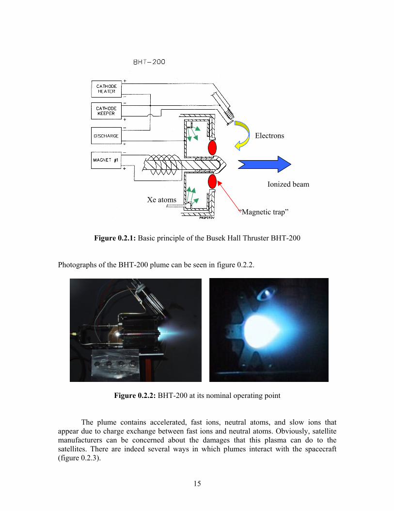
In order to understand what bad effects an electric thruster plume can have on a spacecraft, here is a more detailed explanation of how a Hall thruster works (figure 0.2.1).

1) The cathode emits electrons that are attracted to the anode. As they enter the thruster, they are trapped along the magnetic field lines created by the electromagnet in the regions highlighted in red in figure 0.2.1.

2) On the other hand, the propellant molecules called “neutrals” are brought to the

thruster by feed lines (in green). In our case, the propellant is Xenon. They enter the thruster channel, collide with the trapped electrons and get ionized (Xe+ and Xe++).

3) The ions resulting from this process are accelerated by the electric field that exists between the anode and cathode. They exit the channel and produce the thrust. The plasma beam that is generated is actually not positively charged but quasi-neutral thanks to electrons from the cathode.

15

Figure 0.2.1: Basic principle of the Busek Hall Thruster BHT-200 Photographs of the BHT-200 plume can be seen in figure 0.2.2.

Figure 0.2.2: BHT-200 at its nominal operating point

The plume contains accelerated, fast ions, neutral atoms, and slow ions that appear due to charge exchange between fast ions and neutral atoms. Obviously, satellite manufacturers can be concerned about the damages that this plasma can do to the satellites. There are indeed several ways in which plumes interact with the spacecraft (figure 0.2.3).

“Magnetic trap”

Electrons

Xe atoms

Ionized beam

16

Figure 0.2.3: Plume-spacecraft interactions Solar array and surface interactions: High-energy ions erode the nearby surfaces, and

the sputtered materials can contaminate solar arrays or other sensitive surfaces. Charge exchange plasma and charging interactions: These low energy ions flow back

to the spacecraft and affect the spacecraft potential. They may also contribute to erosion of soft materials.

Optical emissions from the plume could affect sensitive optical instruments.

Communications interactions from plume signature: The plasma and the EM fields

from the thruster may distort the communication signals.

Also, it is important to know the expansion of the plume in order to keep sensitive surfaces out of it. Finally, radiant and conducted heat from the thruster and its plume must be accounted for in the thermal model of the spacecraft.

Extensive studies on the ground have been conducted. But uncertainties persist for

some areas due to facility effects: deposition of material from chamber walls, recirculation of sputtered materials, background gas and background pressure, and geomagnetic effects may change the characteristics of the plasma and mask the real (in-space) behavior of the thrusters. For example, scattering and CEX of plume ions off background neutrals are added to the ions produced in the thruster, and would not be present in space. Also, there is some remaining doubt about the thrust, mainly because the level of vacuum may affect the occurrence or not of a central bright “spike” in the plume, and its appearance is correlated with a noticeable increase in thrust and efficiency: the performance of the thruster in space may consequently be significantly less than measured during ground testing.

Consequently, there is a real need for more in-space data about these issues. The

following paragraph explains the objectives of the ETEEV experiment.

Charge-Exchange Plasma

Plume Expansion

Charging Interactions

Communications Interactions

Solar Array Interactions

Surface Interactions

Plume Signature

17

0.3) Objectives of ETEEV

As seen in the last paragraph, there are indeed parameters for which people seriously doubt that the ground experiments accurately reproduce the operation of the thruster in space. The main concern that we attempt to resolve with the ETEEV experiment on the Space Shuttle is the comparison between data obtained in ground facilities and in-space, in-situ data. It is really a differential experiment to help clear out the uncertainties mentioned above: the ground experiments are much cheaper to conduct, so we need to make sure how accurate their results are. ETEEV would consequently provide both useful science results and a reference for future missions. More precisely, ETEEV will address the following measurements as primary objectives:

Deposition measurements in the plume back plane (i.e. at an angle of at least 70

degrees from centerline), at mid-range distances (10 to 30 cm): this is difficult to obtain in ground facilities because of the interference of the chamber walls and recirculation of sputtered materials.

Erosion, at 60 degrees from centerline and mid-range distances: it is masked in

ground facilities for the same reasons as the depositions. Diagnostic measurements of plasma parameters in the near and mid plume, thanks

to instruments mounted on a moving arm sweeping through the plume: Ion Density and Energy, Electron Temperature, Plasma Potential, Current Density. Extensive data have been taken in ground facilities, so the goal of obtaining these measurements is again a comparative purpose, not doing a complete mapping.

Time and funding permitting, secondary objectives would be to obtain: Thrust measurements for a performance characterization of the Hall thruster at

selected operating points: thrust has never been verified in space, and the measurements taken in the ground facilities tanks may be artificially high because of ingested residual gases adding to the thrust.

Optical observations:

- To verify the existence of a bright “spike” on the centerline of the plume and to evaluate its impact on thrust;

- To check the expansion of the far field plume (farther than 1 or 2 meters), for various orientations of the shuttle ram and geomagnetic field;

- To measure the optical emissions from the plume at a few chosen spectrum lines. An evaluation of EMI emissions susceptible of interfering with communication

signals. We would also measure the pressure and the plasma background in the Space Shuttle Payload Bay in order to characterize the “environment” before, during and after operation of the thruster.

18

Finally, the main advantage of a Shuttle experiment over scientific satellite flights is that the hardware is brought back to Earth after the flight. It can consequently be investigated for changes in its materials or in the way it operates. This possibility of a flight experiment on the Space Shuttle was offered by NASA to the Massachusetts Space Grant.

At this point it is important to note that, although this thesis concentrates on

Hall thruster studies, two thrusters (shown on figure 0.3.1) were originally selected to be experimented on: a Hall Thruster provided by Busek Company, Natick, MA, and a Pulsed Plasma Thruster (PPT). However, the PPT is still optional at this point.

In 2001 this particular Hall thruster (Tandem-200, 200 W, 10.5 mN of nominal

thrust) was selected as the primary means of propulsion for the Air Force satellite Techsat 21, thus making the experiment even more relevant. According to the latest discussions with NASA Goddard Space Flight Center, ETEEV is ranked number 9 on the list of priorities and would have a flight opportunity in late 2004 as a Hitchhiker payload. A demonstration flight of Techsat 21 is scheduled in 2004 as well, so the development studies can be shared: the ETEEV experiment would use the same thruster, cathode, flow system and power processing unit (PPU) as the satellite.

Figure 0.3.1: Pictures of the thrusters

Our team includes many partners as summarized in table 0.3.1 below. The principal investigators are Professors Martinez-Sanchez (MIT) and Gatsonis (WPI), and systems engineering is taken care of by Michael Socha from the Draper Laboratory. We are currently in the process of expanding this “consortium” of institutions and companies to other potential sponsors who would be interested in funding manpower or hardware. For example, as we get closer to the first safety reviews, a full time safety engineer would be valuable for the team.

Busek Tandem-200 Hall Thruster (200W, flight version)

PPT thruster

19

Table 0.3.1: The ETEEV team

0.4) Outline of the thesis As explained in the first paragraph of this introduction (§0.1), my work consisted of three steps that will be reported here: Chapter 1 – An update of the state of the art as regards instrumentation and results of tests in the field of electric thrusters plume/spacecraft interactions and performance, through a review of recent papers. Chapter 2 – An update of the status of the flight experiment design. Chapter 3 – The preliminary design and ground testing of some of the instruments: a Quartz Crystal Microbalance (QCM), a Faraday Cup (FC), a Quadruple Langmuir Probe (QLP), and some optical diagnostics (color videocamera and narrowband filters). The appendixes contain a bibliography, links to the main relevant NASA documents, and manuals for the lab hardware that was used in the testing.

Institution Participants Roles Massachusetts Institute of Technology (MIT)

Prof. Manuel Martinez-Sanchez Anne Pacros, Yassir Azziz Jennifer Underwood, Nida Farid, Jadon Smith

Principal Investigator Graduate Researchers UROPs

Worcester Polytechnic Institute (WPI)

Prof. Nikos Gatsonis John Blandino Jurg Zwahlen, Andrew Suryali

Principal Investigator Asst. Professor Graduate Researchers

Busek Company Vlad Ruby Bruce Pote

Contribute 200 W Hall Thruster

AFRL Edwards Greg Spanjers Contribute QCMs Draper Laboratory

Michael Socha Jareb Mirczak

System Engineering Thrust Balance

Potential Participants:

Michigan Space Grant

Alec Gallimore NPF probe Large vacuum facility

NASA GRC Eric Pencil Contribute PPT? AFRL Hanscom David Cooke Contribute DIDM Instrument

20

21

Chapter 1

Update on the state of the art of electric thruster plume/spacecraft interactions and performance

Lots of experiments have been designed and conducted to attempt to learn more about “operational” characteristics of electric thrusters, particularly about their impact on the spacecraft and their performance. Here is a review of different papers with interesting designs for these measurements.

1.1) Depositions, erosion and plasma instruments

1.1.1) QCM’s Principle

The quartz crystal microbalances (QCM’s) are used to detect very small changes in mass. As explained in reference [1], they have been used in space for erosion and contamination experiments for a long time: the first QCM’s were flown on the Discoverer 26 satellite in 1961 to measure sputtering erosion rates in the upper atmosphere. QCM’s are based on the observation that added mass per unit area (∆m/A) on a quartz crystal increases its inductance and consequently decreases its resonance frequency. More precisely, the crystals used for QCM’s are cut from laboratory-grown crystalline quartz. Depending on the orientation of the cut, different properties are obtained. From reference [1] again, the AT-cut is the interesting one to detect mass changes, because of its frequency temperature stability over a large temperature range. A QCM is consequently composed of a matched pair of AT-cut crystals (one protected, one exposed). The usual range of crystal frequencies is 10 to 30 MHz. Two improvements were made to this first patented design. The TQCM (Thermoelectrically-Cooled QCM)

22

enables the user to control the temperature of the QCM between 100 and –60°C, to study the effects of temperature changes on the adsorption and desorption rates. Also, they can help studying the composition of the depositions: for example, if the TQCM temperature is above the vaporization temperature of a certain contaminant, then whatever depositions the TQCM collects will be free of this contaminant. Finally, the CQCM (Cryogenic QCM) extends the operation temperature range to -200°C by cooling the crystals with a cryogenic fluid. The thermoelectric device of the TQCM is replaced by an external, passive cooling system and temperature is controlled with a resistance heater.

QCM operations

They are explained as well as data analysis is explained in reference [2]. The QCM output is the “beat frequency” (i.e., the difference between the reference crystal and the test crystal):

where Sf is the crystal sensitivity, τ the film thickness, ⋅

δ the rate of deposition. The two oscillations are mixed and the beat frequency signal is designed so that increase in frequency means increase in mass. So the reference frequency must be higher than the test crystal (cf above: frequency decreases with added mass). There are 2 advantages to this output: it is in the KHz range so it is less attenuated than MHz signals in long cables (in case the QCM is located remotely from the telemetry system); and beat frequency cancels out frequency fluctuations caused by ambient temperature changes. Consequently, the resolution on the thickness of the deposited film is of the order of an angstrom (less than a monolayer of atoms!). Finally, the issue of temperature control was addressed in reference [3]: when exposed to the sun, there is a frequency change (as high as 50 to 150 Hz on rotating spacecraft!!) because solar thermal radiation strikes the exposed crystal and not the reference crystal, and there is a temperature sensitive component in the crystals used. Also, heating causes mass deposits to evaporate. The solution investigated is to place reference and test crystal side by side and cover the reference one by a sapphire window (blocks any mass flux but allows thermal radiation to strike it). The frequency response to thermal variations was reduced by 82% so the performance is improved (and data is easier to interpret). Examples To date, QCM’s have been used a lot for contamination and erosion studies, but only a few times specifically for thruster plume effects characterization. A couple of examples are the ESEX, SPIRET and STENTOR experiments where QCM’s were part of a complete thruster diagnostics package (see section 1.4 of this thesis).

Reference [2] deals with the MSX satellite (1996) with the SPIRIT III telescope (CQCM MK-16 mounted next to primary mirror). In the 60 first days on orbit, CQCM

tSSAmSF fff ∆==

∆=∆

⋅δρρτ

23

mass accretion was rapid because very low temperature (20K) caused condensation of oxygen, argon, nitrogen, water vapor. Then deposits thickness stabilized around 155 Å and additional accretion was minimal. Also 4 TQCM’s (modified MK-10) were placed on external surfaces, operated around –50ºC and have shown accumulations between 7 and 134 Å. The ones with solar panels in their field of view have shown the largest deposition rates.

Another example of flight TQCM/CQCM system was flown as a part of the

IECM experiment (Induced Environment Contamination Monitor) on early Shuttle flights like STS-2 (November 1981). It was designed to check for contaminants in and around the Space Shuttle orbiter payload bay that might adversely affect delicate experiments onboard. It is a multi-instrument box as seen on figure 1.1.1.1:

Figure 1.1.1.1: IECM grappled by Shuttle Robot Arm

The orbital phase on STS-2 lasted about 53h. The TQCMs (Faraday Laboratories, Inc.) had sensitivity of 1.56x10-9 g/cm2/Hz and were operated at 4 preset temperatures: +30, 0, -30 and –60ºC. Note that these early analyses did not take into account Orbiter-related contamination events (thruster firings, water dumps, flash evaporators). But it would be interesting for us to get the full set of data that was recorded on these flights in order to compare with the depositions we will be measuring. Finally, paragraph 3.2 of this thesis contains information on the MK-16 CQCM from QCM research since it is the model the MIT Space Propulsion Laboratory owns. Results

As reported in reference [4], the most important results for us are:

- Some frequency variations are due to transitions sun/shadow (sudden changes in T); also a large frequency increase was observed 2 hours and 18 minutes after launch, corresponding to the opening of the payload bay doors;

- For the most part, molecular accumulation remained at low levels below 1 ng/cm2/min; some of the rates were negative, indicating that desorption was more important than adsorption.

CQCM’s TQCM

Passive array

24

1.1.2) Witness plates Principle

These instruments are samples of materials that are exposed to thruster plumes in

order to measure erosion and deposition rates. Usually a part of the sample is protected to provide a control during analysis. Materials commonly used (and particularly interesting for us) include representative samples of solar array materials: solar cell cover glass, solar cell circuit conductors. Also metal and other usual construction elements are reported. Critical surfaces potentially subject to erosion are Anti Reflective coatings (whose removal can result in 2% degradation of solar cell performance) and conductive solar cells interconnection materials (erosion degrades performance by increasing resistance).

Predictions

Models for erosion are based on the relationship between sputtering and ion

current and energy of the ions hitting the surface (references [5] and [6]). The velocity with which a surface is removed (λ) is given by

viiv SjSNth '),( ×=Φ×=

∆∆= ελ &

where ∆h is the step height between the control and the exposed part of the sample, ∆t the duration of exposition, N& the flow rate of particles to the surface, Sv the volumetric sputtering coefficient depending on particle energy εi and angle of incidence Φ, and ji the ion current at thruster exit. S’v is Sv transformed to electrical values (in cm3/C) because the current density j is linked to N& by j= N& x charge q.

Using εi ~ e Vd (where is Vd the discharge voltage), reference [5] finds λ = 5x10-2 Å/sec at 45º from the centerline and 1 meter from the thruster. So a 7x10-3 cm change in the surface thickness is predicted for 4000 hours of operation.

In reference [6], the ion current ji is estimated by a Lorentzian fit over

experimental results. Also the linear fit S’v = AE+B was used, where E is the ion energy (also obtained by a fit on experimental data), and A, B are coefficients depending on material. Predicted erosion rate of thruster insulator was then 3x10-1 Å/sec at 40 degrees, 3x10-2 Å/sec at 90 degrees. Deposition rates were evaluated by assuming that the volume of deposited material equals the volume eroded from the discharge chamber insulator: 8x10-3 Å/sec at Beginning Of Life (BOL), 2x10-3 Å/sec at End Of Life (EOL). There is indeed a difference between BOL and EOL results because of decreasing erosion in the discharge chamber as the thruster ages.

The agreement between these predictions and experiments is usually good except

for high divergence angles because predicted current takes into account CEX ions whereas in reality they are not energetic enough to erode.

25

Examples Most experiments in the literature are organized in the same way. The samples are

equally spread at a constant radius of the thruster exit as seen on figure 1.1.2.1. Moreover, some or all of them are protected by collimators to avoid contamination by materials sputtered from the vacuum chamber wall. The design of these collimators involves making sure that the sample still has the thruster in its line of sight. Also, they should be made out of a material that is very resistant to sputtering like tantalum so that as little deposition as possible comes from collimator sputtering. A diagram of the collimators used in reference [8] is on figure 1.1.2.2.

Figure 1.1.2.1: Disposition of the samples (from reference [8])

Figure 1.1.2.2: Collimator design (from reference [7])

Thruster centerline

26

After exposure, the analysis of the samples usually consists of several measurements:

- Mass variation measured with an electronic balance - Profilometry to determine the step height - Auger spectroscopy for chemical analysis of the depositions - Optical properties (transmittance, absorbance…) determination - For solar cells connectors, changes in resistance are monitored.

Results

Reference [5] used a Stationary Plasma Thruster SPT-100 (1350 W, ISP 1630 sec,

50% efficiency) with samples at 0.6 m, protected by conical collimators of 15 cm, for 95 hours. The materials were solar array cover glass (typical from US satellites), glass and metal (from the Russian investigators). Erosion of surfaces and loss of transparency (less than 6%) was observed. For angles of less than 45º from the centerline, there was a clear imprint of collimator aperture, which shows that ion trajectories in the flow are linear.

Reference [6] used the same thruster as [5] but samples were 1 m from the

thruster and exposed for 200 hours. Materials were cover glass (MgF coated borosilicate glass with 5% cerium dioxide), and solar array interconnect material (silver coated kovar connectors, and silver foil strips). There was a noticeable mass loss for all samples, especially silver which is very sensitive to sputtering, for angles 0 to 70º. Elements identified in the depositions were those of the collimators, thruster insulator (boron, nitrogen), and propellant; no facility contamination was noticed. Finally there was a change in optical properties for angles of less than 60º (absorbance increases, transmittance decreases). In terms of solar array impact (using the data for divergence angles greater than 60º, because thrusters are usually canted from the solar panels orientation):

- Optical performance was not degraded to a measurable extend. - There was an increase in circuit resistivity (because cross section of connectors

decreases with erosion). But worst-case erosion is 3 µm over life (while the typical thickness is 10 to 100 µm) and concentrated on small areas of array so it would not cause problems for typical satellites.

- Erosion thickness of cover glass was less than thickness of cover glass Anti Reflective (AR) coating. Reference [7] reports 200 hour, EOL tests on SPT-100. Test A used samples at 1

m for 30 to 90º divergence angles, and test B also studied the influence of ion incidence by changing the orientation of the samples with respect to the flow. The samples were coated CMX cover slides for A, polished quartz and AR coating (Magnesium Fluoride) CMX slides for B; CMX is a ceria-doped borosilicate used to cover silicon solar cells. The analyses enabled the authors to identify three regions:

27

1) A high erosion region for angles < 65º (and peaking as one gets closer to the centerline): partial to complete AR removal happened there, with a maximum rate of 7.3x10-1 Å/sec at 30 degrees.

2) A contamination region for angles between 65º and 80º (peaking at 75º), where

properties change due to film contamination (7.2x10-4 Å/sec of depositions at 75º).

3) A peripheral area (angles >85º) where changes were negligible.

Also, the influence of incidence was not discernable for most of the samples. A

measurable decrease in surface resistance (109 instead of 1010 Ω) was noticed on one of the samples in the deposition region but not to a problematic level.

Finally, in reference [8] the set up was very similar, but using a 3 kW thruster, with Solar cell cover glass (100 microns thick with AR coating), RTV silicone samples and Kapton samples were exposed for 100 hours. Confirming the experiments above, the source of contamination was primarily boron from the thruster insulator parts. Also materials from the erosion of the samples (zirconium and silicon from AR coating for example) were found. Collimators worked well to prevent materials from the facility to deposit. Depending on the position of the sample, mass loss varied from 0 to 9.1 µg/cm2, (~ 2.8x10-3 Å /sec) and step height from 300 to 379000 Å. Again reflectance increased at the expense of transmittance.

The main results to remember for these ground studies are:

- Erosion and deposition rates vary a lot between BOL and EOL; - Three regions can be identified (erosion, deposition, and peripheral) - Solar array impact can be minimal with a proper positioning of the thruster.

We found no literature about witness plates in space. Using these instruments indeed implies that the samples must be retrievable for analysis, because of the complex diagnostics involved such as profilometry and spectroscopy. Hardware retrieval is doable only with the Space Shuttle, so we would apparently be the firsts to do witness plates in space.

Usually witness plates measurements are coupled with plasma diagnostics

because as we just saw, it is important to know ion current and energy to make predictions about the erosion rates. The following paragraph consequently reviews Faraday Cups (FC) and Retarding Potential Analyzers (RPA).

28

1.1.3) Faraday cups/ Retarding Potential Analyzers Principle

These instruments are used to measure the distribution of current density (with a FC) and ion energy (with a RPA) in plasmas. The measurements are usually used as inputs in models to quantify the impact of plumes on spacecrafts as seen in the previous paragraph but also to indirectly determine the thrust. They can be mounted either as stationary probes or on a mechanical arm sweeping through the plume.

Let us address the FC first. The underlying physical principle of a Faraday Probe is that ions hit the face of the probe so that electrons in the metal (supplied by the outer power source) go to the probe face to neutralize collected ions. The current created in the electrical circuit is therefore equal to the ion current at that location. Dividing by the probe area then gives the current density. This gives no information on number and mass of the ions so we need to assume a uniform charge state distribution. Faraday Cup design

Two major shapes emerge in the literature on probes used specifically for electric

propulsion plasmas. References [9] and [10] use a “current trap” design as seen on figure 1.1.3.1 (from reference [10]).

Figure 1.1.3.1: Current trap (from reference [10])

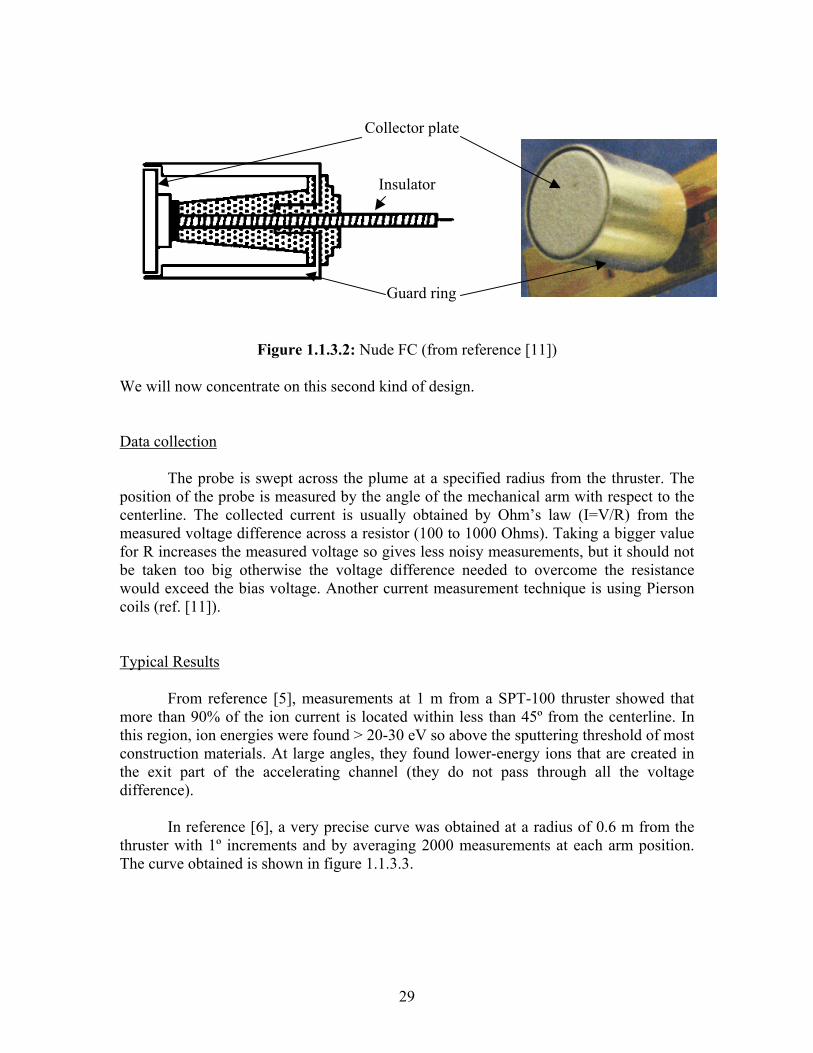
References [5], [6] and [11] use flat disk probes with guard rings, surrounded by a grounded support (for electrostatic shielding), and biased negatively in order to repel electrons and attract ions. The material used for the disk is chosen for its low secondary electron emission (typically Molybdenum or Tungsten). The bias voltage is usually of the order of – 20-30 V in order to ensure that the probe is below the plasma potential and that the probe is in the ion saturation region. The guard ring minimizes the effect of ions hitting the probe elsewhere than on its face. Figure 1.1.3.2 shows a diagram and a picture of such a “nude” Faraday probe (from reference [11]).

Faceplate Aperture

Current trap

Shield

29

Figure 1.1.3.2: Nude FC (from reference [11]) We will now concentrate on this second kind of design. Data collection

The probe is swept across the plume at a specified radius from the thruster. The position of the probe is measured by the angle of the mechanical arm with respect to the centerline. The collected current is usually obtained by Ohm’s law (I=V/R) from the measured voltage difference across a resistor (100 to 1000 Ohms). Taking a bigger value for R increases the measured voltage so gives less noisy measurements, but it should not be taken too big otherwise the voltage difference needed to overcome the resistance would exceed the bias voltage. Another current measurement technique is using Pierson coils (ref. [11]).

Typical Results

From reference [5], measurements at 1 m from a SPT-100 thruster showed that more than 90% of the ion current is located within less than 45º from the centerline. In this region, ion energies were found > 20-30 eV so above the sputtering threshold of most construction materials. At large angles, they found lower-energy ions that are created in the exit part of the accelerating channel (they do not pass through all the voltage difference).

In reference [6], a very precise curve was obtained at a radius of 0.6 m from the

thruster with 1º increments and by averaging 2000 measurements at each arm position. The curve obtained is shown in figure 1.1.3.3.

Collector plate

Insulator

Guard ring

30

Figure 1.1.3.3: Typical current density curve (from reference [6]) Collimated Faraday Probe

This is a variant of the traditional FC design. The purpose of collimating a FC is

to obtain true ion current density profiles independently of the pumping speed of the vacuum facility (i.e. independently of the background pressure). Indeed, as reported in reference [11], Hall Thrusters move to higher powers and higher flow rates while facilities cannot really improve their pumping speed in the near future. A perfect vacuum is not always necessary since the pressure in LEO is around 5x10-6 and 5E-10 torr in GEO. But some suggestions exist about what is acceptable in terms of pressure depending on the type of testing that is done (table 1.1.3.1):

Type of testing Maximum acceptable pressure

Performance 5.E-05 EMI 5.E-05

Farfield (<1.2 m) 5.E-05 Life and spacecraft contamination 5.E-06

Table 1.1.3.1: Acceptable pressures for SPT-100 testing

(from Randolph, et al., IEPC 93-093, quoted in reference [11])

The problem of background pressure is that it creates CEX products (fast neutrals and slow, random ions as explained in the introduction) in the plume. CEX happens also in the exit plane but that would happen in space too, so it is not what we are concerned about here. The idea of the collimator is to create a filter to the low-energy, random CEX ions because as the collimator reduces the field of view of the collecting plate, only ions with a velocity vector in a small solid angle are collected. Figure 1.1.3.4 is the collimated FC design investigated in reference [11]:

Cur

rent

den

sity

(mA

/cm

2 )

31

Figure 1.1.3.4: Collimated FC (from reference [11]).

The authors compared the results obtained with a nude and a collimated FC. They

used a scale factor to account for the fact that some high-energy ions are also unintentionally blocked by the collimated design compared to the nude probe. The experimental set up can be seen in figure 1.1.3.5:

Figure 1.1.3.5: Electrical diagram for Faraday Cups (from reference [11])

Different cases were investigated: floating or biased guard ring for the nude; floating or biased collimator and guard ring for the collimated. It was hypothesized that the effect of the collimator would be the same as a decrease in chamber pressure, i.e. the current density would be unaffected in the region between ±30º from the centerline, while the outer regions of the plume would exhibit a lower current density due to lower CEX. Unfortunately, there was a 33 to 48% difference between the nude and the collimated design (the collimated being lower); CEX filtering would account for only 6 to 10 % of that, and what is more, the central ±30º zone unexpectedly showed a decreased current density.

The conclusion of the study was that unexpected processes must happen within

the collimator. Mechanisms that could account for this attenuation (CEX collisions inside the collimator, scale factor errors, reduction of the aperture area by the sheath) were ruled out. So more study is needed in order to understand the collimated Faraday Cup.

Collimator

Collector

Close the switches to bias guard ring and collimator

Nude FC

Collimated FC

32

A configuration that was not tested but could be interesting is the case where the

collimator is allowed to float in the plasma while the guard ring and the collector are biased. This may be a way to limit the effects of the collimator on the plasma while ensuring collection of the ions.

Retarding Potential Analyzers

Finally, we will briefly address RPA design and results. It functions the same way as a FC but an RPA uses a series of electrodes to selectively filter out ions of varying energy, yielding an ion current which depends on the potential of the electrodes: the higher the positive potential, the more energetic the ions have to be to reach the collecting plate. The applied potential is therefore called “ion retarding potential”. Figure 1.1.3.6 and 1.1.3.7 show the design used in [13].

Figure 1.1.3.6: RPA (from reference [13])

Figure 1.1.3.7: Potential profile in the RPA (from reference [13])

Ground

Ion retarding potential

FE: Floating Electrode ERE: Electron Retarding Electrode IRE: Ion Retarding Electrode SESE: Secondary Electron Suppression Electrode FG: Floating Grid ERG: Electron Retarding GridIRG: Ion Retarding Grid

33

Results of [13] showed the existence of high-energy ions (>284 eV) and gave energy distribution curves. Comparison with other RPA designs pointed out several issues of RPAs:

- Large aperture and closed back result in high pressure build up (in the mtorr range!), then in more CEX and consequently a broadening of the ion energy distribution;

- Space charge limits of the measured current; - Defocusing of the beam by the series of grids also introduces errors.

The first of these problems was tackled effectively in [13].

For the scope of this thesis, we will concentrate on Faraday Cup design. To sum up this paragraph, results for the current density should lead to a curve similar to that of figure 1.1.3.3. Major design issues are:

- Insulating and biasing the different parts; - Ensure not too noisy data collection; - Collimated FC design and interpretation (particularly prevent pressure build up in

the collimator). Other plasma parameters measurements like densities, plasma and floating

potentials, and electron temperature will now be reviewed.

1.1.4) Langmuir Probes / Emissive probes Principle of Langmuir probes (LP) Cylindrical Langmuir probes are made with a metallic wire insulated except for a small part called the “tip”. This wire is put in contact with the plasma and because ions and electrons hit the tip of the probe, a current is collected and depends on the voltage bias applied to the probe (see figure 1.1.4.1).

Figure 1.1.4.1: Langmuir probes principle (from reference [14])

The collected current with respect to the voltage is a curve shown in figure 1.1.4.2 (from Carney, L. M., Keith, T. G., “Langmuir Probe Measurements of an Arcjet Exhaust”, AIAA 87-1950, 23rd AIAA/SAE/ASME/ASEE Joint Propulsion Conference).

34

Analyzing the curve enables to determine plasma parameters like Te (electron temperature), ne (electron density), Vf (floating potential) and Vp (plasma potential).

Figure 1.1.4.2: I-V characteristic for a Langmuir Probe Two methods exist to find the I-V curve. One could either:

- Use a probe with a single tip and change the voltage value: this technique called the voltage sweep gives as many points on the curve as there are voltages values but requires an adequate power supply;

- Use a probe with three tips, one floating and two biased with respect to each other. This is called a triple probe and gives 3 points on the I-V curve with no need to change the biases. This is all that is needed to determine the curve in quiescent plasma. By adding a fourth tip it is also possible to determine the flow velocity. Figure 1.1.4.3 shows such a “quadruple Langmuir probe”.

Figure 1.1.4.3: Quadruple Langmuir probe (from reference [15])

Examples of studies and results From what has just been seen, Langmuir probes are not very hard to build. But their main difficulty is in data interpretation, because to deduce Te, ne and Vf from the obtained current we need to choose an appropriate model for the plasma we are surveying: strong or weak magnetic field, collisionless or not, flowing or not, etc.

When the probe bias Vis very positive, all ionsare repelled and onlyelectrons are collected.

When the probe biasis very negative,electrons are repelledand ions are attracted.

Vp

35

Reference [16] deals with a LP experiment in a PPT plume. They measured electron temperature and density with a triple Langmuir probe. Probe 2 was allowed to float in the plasma while a voltage Vd3 was applied between probes 1 and 3. Then they measured the voltage difference between probes 1 and 2 (Vd2), and the current I3 collected by probe 3 (figure 1.1.4.4).

Figure 1.1.4.4: Triple Langmuir probe circuitry (from reference [16]) Using a combination of ion current collection models they find implicit equations

for Te and ne. Problems encountered in the measurements were:

- Probe contamination: since the PPT Teflon plume is very dense, the probes were covered with a dark deposit. So they had to clean tem using a glow-discharge;

- Noise in the data: the origin of this noise is both electromagnetic interferences and low oscilloscope resolution. It was possible to reduce it by applying statistical filters.

Reference [17] deals with the effect of ion drift flow perpendicular to a cylindrical

triple LP on measurements in a MPD plume. The triple probe had the same configuration as in reference [16], and they varied the angle between the probe and the thruster axis. For angles of 60 and 90º, the collected current was greatly increased because ions are collected not only by diffusion but also from convection. What is less obvious is that Te was also affected. The main conclusion was that accurate profiles of ne and Te can be obtained by sweeping the LP through the plume at different angles from the thruster axis, selecting only the measurement giving minimum current at each location (this value corresponds to the best alignment of the probe with the flow).

Reference [14] also considered a supersonic flowing plasma but in a Hall thruster

plume (figure 1.1.4.5). The thruster was a SPT-70 (660 W power, 40 mN thrust).

36

Figure 1.1.4.5: LP in flowing plasma (from reference [14])

A formula for the total current collected by the probe in the electron-repelling mode (V<Vp) was derived: it is the sum of the electron current

ee

ee S

kTVpVecneI ))(exp(

4−=

and the ion current )1( siiei fSvenI += . S is the collection area, taken to be the total probe area for electrons (Se), and its projection on a plane perpendicular to the flow direction for ions (Si). Since this projection changes with the location of the probe when sweeping across the plume, it has to be measured. Also, fs accounts for the expansion of the sheath (“first order estimate based on empirically determined slope for the ion saturation region”). The ion velocity vi can be predicted based on the discharge voltage Vd and the beam energy efficiency ηe (taken to be 0.88):

i

edi m

eVv η2=

The case of the electron-attracting probe (V> Vp) is modeled using the orbital

motion limit theory: the ion density is unaffected by the bias, so it is constant around the probe, and there are no potential barriers for electrons (as if the sheath was infinite). Whether electrons reach the probe or not depends only on their trajectories. The electron and ion currents are then:

ee

pee S

kTVVecneI )

)(1(

4−

+=

and iiei SvenI = Experiments were done with a triple LP in a similar setup as the other references cited above. I-V curve, ne, Te and Vplasma “maps” were obtained.

Ion beam Wake region

SheathPlasma region

37

Finally, reference [15] investigates perturbations induced by Langmuir probes on Hall thruster operations. A model for thermal evolution of a LP in a Hall thruster plume was developed and experiments were conducted on a SPT-70 with a quadruple LP. Two sets of data were taken:

- With the probe outside of the discharge chamber, the flux was not energetic enough to ablate probe material and probe “survival” was not an issue, but the presence of the probe affected the local plasma parameters.

- With the probe inside the thruster, not only modifications of parameters but also ablation of the probe (“burning”), and operational characteristics of the thruster were modified.

Since our use of Langmuir probes would be to survey plasma parameters in the plume, only the first kind of perturbation is a concern for us. Emissive probe

Figure 1.1.4.6: Emissive probe These probes are made of a filament that is heated up (figure 1.1.4.6). It starts

emitting electrons. Similarly to the Langmuir probe, the emissive probe is biased to different voltages. For a high positive voltage applied to the probe, the electrons are attracted back to the probe and a current is collected. But if Vprobe<Vplasma, the electrons are lost to the plasma, they escape and do not come back to the probe: the I-V curve exhibits a big current drop. So the I-V curve is similar to the Langmuir probe one, but with a more noticeable kink at the plasma potential. So emissive probes are useful to get a more precise value of the plasma potential.

As a summary, the major results and design issues that concern us for the use of

Langmuir probes are: - Handling noisy data - Interpreting the data in a flowing plasma - Quantifying the perturbation of the probes on the plasma.

Now that we have reviewed plasma diagnostics applicable to achieve the primary

objectives of our ETEEV mission, we will look into instruments for our secondary objectives.

Insulator Heated filament

38

1.2) Performance

Principle “Performance Evaluation” usually stands for tests where performance metrics are measured and calculated for different values of the thruster and environmental parameters. Parameters commonly used for Hall thrusters are: - Flow in the thruster itself, flow in the cathode and thus total flow m& - Discharge current, voltage and power P - Magnet power - Tank pressure Performance metrics are: - Thrust T measured by a thrust stand

- Specific Impulse (ISP) calculated by the formulagm

TIsp&

=

- Efficiency η calculated by Pm

T&2

2

=η

Examples References [18] and [19] report performance testing on an SPT-140. The papers first describe the operating conditions: pumping speed of the vacuum chambers, power supply system, and propellant used. In the first of these references, an inverted pendulum thrust stand was used; it has to be precisely calibrated but due to zero drift, the uncertainty in the thrust measurements is around ±1.5%. Other complementary instruments were used in the second paper, like a Faraday Probe and a thermocouple to provide a reference of the thruster temperature.

Results In reference [18], a general performance assessment was done by plotting ISP versus thrust. Then, different operating points having in common the same thruster power were tested. It was usually believed that higher discharge voltages resulted in higher ISP and higher discharge currents resulted in higher thrust, but these experiments showed these hypotheses were not valid: as the discharge voltage was dropped from 240 to 200 V, the thrust increased, but for lower voltages the thrust was lower than that at 200V. In reference [19], a first performance evaluation was done at minimum background pressure attainable in the facility used, and magnet current was optimized at each condition for maximum thrust. Discharge voltage had a strong influence on ISP, and

39

thrust was a near-linear function of discharge power. Then in a second test, the background pressure was varied. In general, higher pressure induced a net decrease in supply flow in order to maintain the same discharge current and thus to stay at a fixed power. Since flow is in the denominator of the formulas for ISP and η, this induces an apparent increase in ISP and efficiency. Consequently, the real thrust and ISP obtained in space (where background pressure is lower than in the best ground facilities) may actually be lower than those obtained in ground facilities. It seems therefore important to conduct in-space performance assessment of Hall thrusters, which involves the design of a thrust stand for flight (see paragraph 2.3).

1.3) Electromagnetic Interference (EMI) and Optical Emissions

Principles of EMI experiments Electromagnetic interference is one of the drawbacks of electric propulsion that

satellite manufacturers fear the most (especially for communication satellites). Indeed, reference [20] shows that as early as 1987, radiated emissions were a concern for satellite integration of electric propulsion devices: this paper establishes a huge database of EMI results from studies, ground tests, and missions. Moreover, a lot of recent papers (references [21] to [30]) show a renewed interest in this matter as more and more thrusters are ready for flight integration and must meet more and more restrictive standards.

As EMI experiments are not confirmed yet for the ETEEV payload, we will only

do a quick review of the different experimental setups from the referenced papers. Reference [27] details methods for this kind of investigations that would be interesting to look at in more detail before going into a design phase if we finally do. For instance, three types of facilities used for EMI are detailed in this reference:

a) Standard anechoic chambers with the thruster mounted in it; a compact vacuum

chamber of radio-transparent material is connected to the nozzle of the thruster: these facilities are complex but provide the most adequate measuring of the thruster self-emission;

b) Vacuum chambers with walls covered with radio-absorbing materials (not

influencing the vacuum quality): quality of the results is good but it is difficult to secure the anechoic elements in a regular vacuum chamber;

c) Metal vacuum chamber: despite the high level of reflections on the metallic walls,

they provide an easy setup that enables users to fulfill most of the necessary measurements.

40

Note that (a) and (b) are different because in the first case, only the region downstream of the nozzle is in vacuum, while the rest of the setup is in an anechoic chamber, not a vacuum chamber; in (b), a “classic” vacuum chamber is used, only modified to resemble an anechoic room.

Two kinds of experiments are usually done (reference [20]). The first one aims at

verifying that radiated emissions from the thruster and its plume do not pose any problem to susceptible spacecraft systems. Military standard MIL-STD-461 (B, C, E, E being the latest version) establishes EM emissions limits and susceptibility requirements; MIL-STD-462 defines test procedures and measurement techniques. A typical set up is shown on figure 1.3.1.

Figure 1.3.1: Experimental setup for emissions verification (from reference [27]) The other kind of EMI experiment (again from reference [20]) is to evaluate

transmission impacts. It is indeed often necessary for uplinks and downlinks signals to travel through a portion of thruster plumes. Plume-signal interactions include:

- Reflection of the transmitted signal by the plume; - Attenuation and phase shift of the signal as it passes through the plume; - Generated noise on both signal amplitude and phase.

A typical set up is:

Figure 1.3.2: Setup for transmission experiments (from reference [24])

41

To understand EMI experiments that are done, it is useful to know how the signals are called depending on their frequency (see table 1.3.1).

Radar Band Frequency Notes HF 3 - 30 MHz High Frequency

VHF 30 - 300 MHz Very High Frequency UHF 300 - 1000 MHz Ultra High Frequency

L 1 - 2 GHz S 2 - 4 GHz C 4 - 8 GHz X 8 - 12 GHz Ku 12 - 18 GHz K 18 - 27 GHz Ka 27 - 40 GHz mm 40 - 300 GHz Millimeter wavelength

Table 1.3.1: “Bands” definitions

Examples and Results

For radiated emissions, [21] showed that for a 660W Hall thruster, electric field measurements were above the MIL standard below 300MHz. This is of little concern since communication links operate mainly in the Ku and Ka bands.

Reference [28] is particularly interesting for us because it studies the EM

emissions from the BHT-200 Hall thruster (the one we have in the MIT Space Propulsion Laboratory). The facility they used is the following:

Figure 1.3.3: BHT emissions experiment facility (from reference [28])

42

The goal was to survey the radiated electric fields from 10 kHz to 18 GHz following MIL-STD 461E specifications, as a function of thruster parameters (discharge voltage, anode flow rate, etc). The main conclusion was that the MIL standard was exceeded by up to 60 dBµV/m on a significant range of frequencies (10 kHz to a few hundred MHz). Figure 1.3.4 shows the BHT emissions for the nominal discharge voltage compared to the MIL standard. Also, EM emissions are linked to plasma instabilities and are not a strong function of the power of the thruster: the more stable the anode current, the lower the radiated emission.

Figure 1.3.4: Emissions at nominal discharge voltage for various anode flows ([28]) For transmission impacts:

Reference [22] studied EM wave scattering of a 17 GHz signal and showed a discrepancy between model predictions and Hall thruster measurements: the model did not correctly predict the power spectral density of the 17 GHz signal transmitted across the plume, especially the second or higher order harmonics attenuations. A better agreement was found by taking into account different kinds of instabilities occurring in the SPT acceleration channel. Reference [23] experimented with signals at 17 and 34 GHz on a P5 Hall Thruster (5kW). They measured a phase shift of up to 30º, and an attenuation of 1.2 dB for the 17 GHz signal and 0.5 dB for the 34 GHz signal. By comparing these results with other tests on other thrusters, they showed that EMI depended a lot on the thruster and on operating conditions.

43

Reference [24] did experiments on S band signals (showing up to 50º phase shift) and on X-band signal (less than 15º phase shift). Numerical simulations gave attenuation and phase delay for different kinds of thrusters. In [25] and [26] a ray-tracing code (“BeamServer”) is developed and used to trace amplitude, phase and path of a ray individually through a plasma plume. Finally, studies of in-flight impacts on communications are reported in references [20] and [24]. For example, the S-band downlink signal was interrupted when operating a MPD arcjet in the Electric Propulsion Experiment (EPEX) on the Japanese SFU-1 satellite in 1995 (it is believed that the pulsed plume with dense plasma delayed the microwave phase).

Optical Emissions This kind of emissions are particularly important for satellites containing optical sensors (for example, space telescopes). It can also be used for diagnostic purposes (i.e. to get insight in microscopic phenomena by a non intrusive technique).

For example, [29] studied the optical emissions thanks to optical fibers placed along the discharge channel of a SPT-50, as well as 1 mm and 21 mm downstream of the exit plane. These results are taken as a baseline for our optical emission experiment (see paragraph 3.5).

Finally, reference [30] considers a model to evaluate the emissions in visible

wavelengths of a Xenon Hall thruster plume. By examining a set of possible reactions between neutrals, electrons, single and double Xe ions, and by using statistical physics considerations, they analyzed the different processes contributing to Xenon particle level populations. Also, radiation excitation processes due to residual background gas could be sorted out which resulted in a extrapolation of ground experiments to in-space operation of Hall thrusters. The radiation intensity in space (predicted by the model) appeared to be less than the one measured in vacuum chambers. Finally, maximum radiation intensity integrated over the visible spectrum was predicted of the order of 10-2 W/m2.sr for a D-80 Hall thruster with anode layer (TAL) along the line of sight crossing the thruster axis at a distance of 22.5 cm. After having detailed the instruments we plan to take on board of the ETEEV experiment, we will review other diagnostics packages for recent space experiments.

44

1.4) Flight diagnostic packages Several electric propulsion flight experiments have already taken place, all on unmanned vehicles (scientific satellites). In this paragraph we will concentrate on three of them (ESEX, Express and STENTOR) and detail the instruments they used. The first experiment of this kind was carried out on the interplanetary spacecraft Deep Space One, whose main propulsion system was a 30 cm ion engine. Details on the diagnostics package can be found in reference [38] (page 46).

ESEX (Electric Propulsion Space Experiment)

It was designed, launched and operated by the United States Air Force in 1999. As reported in reference [31] it was a space demonstration of a 30 kW ammonia arcjet thruster. The firings of the thruster were timed so that they would occur over two ground sites to facilitate ground-based observations. The mission had 4 main objectives:

- Optical observations: they were made using the ground-based 1.6 m

spectrograph/telescope at the MSSS (Maui Space Surveillance Site). The objective was to characterize the emitting excited states spectroscopically and spatially. Despite poor weather conditions, the principal features agreed with ground tests (for example, H lines dominate the spectrum). An on-board still frame video camera was also available, and intended for diagnostics for anomalous operations. It was expected to show the extent of the emitting part of the plume but at full power the plume was too bright.

- Electromagnetic interactions: these tests included measurements from on board

antennas, communication bit error rate tests and verification of uplink/downlink signal integrity. Emissions were measured in the S and X bands; error rates were less than 2 bits in 10000.

- Performance: the ∆V was measured by 3 different techniques: an onboard

accelerometer, tracking and an onboard GPS receiver. The thrust was found to be 1.93 ± 0.06 N.

- Contamination measurements:

- Four TQCM sensors were positioned on the ESEX platform to measure mass depositions. No deposition was attributable to the steady-state operation of the arcjet.

- Four radiometers measured thermal flux from the firings: only the one placed closest to the thruster showed degradation of the sensor material.

- Finally, a sample of solar array segment was placed along with one of the TQCM’s and two of the radiometers in a so called “witness tower” near the thruster exhaust. The performance of the solar cells was tested. It showed an overall 3% degradation over the 60 days where the arcjet firings occurred.

45

Problems that happened in ESEX were linked to a battery anomaly and an ingestion of liquid NH3 in the plenum tank. The instruments themselves performed correctly.

Express (Russian geosynchronous communication satellites) As reported in reference [32], this experiment consists in two satellites, Express-A #2 and #3, launched in March and June 2000 respectively. They are equipped with 4.5 kW Hall Thruster systems (several thrusters and cathodes for each satellite). On-board sensors are: For Express-A #2:

- 3 electric field strength sensors, - 2 ion current density sensors (two-grid Faraday Probes).

For Express-A #3:

- 3 electric field strength sensors, - 2 four-grid RPA’s, - 2 three-grid RPA’s, - 2 pressure sensors (“inversion-magnetron” type).

Also, on both satellites, communication signals were monitored to check for interferences. Results of some of these measurements are presented in reference [32]:

- The effective thrust on-orbit is less than that measured during acceptance testing (8% less for most of the thrusters). However, the effective thrust increased over time: over the first 24 hours on orbit, the performance increased gradually to a steady state value. Momentum transfer due to plume impingement caused disturbance torques, up to 14.2x10-3 N.m on the y-axis (pointing westwards);

- No anomalous performance of communications (in the C and Ku bands) was detected;

- Measured ion current density did not agree well with ground test data nor calculated values. As we will see later, this is because the data was extrapolated to values at 1 m from the thruster using a 1/r2 relation for the decay of current density with distance, in order to simplify the data comparison, and this law is not accurate for the far-field plume;

- Measured ion energy 3.8 m from the thruster at an angle of 8º was 250V while model prediction was 230V, which is quite a good agreement;

- The pressure sensors operated only 8 hours before their power supply failed, but the data taken agreed well with previous measurements that showed the pressure on a geosynchronous satellite would stabilize at 2x10-8 torr (when the thrusters are off) after 10 to 15 days;

- Electric field strength was recorded and stayed between –2 and 2 V/m most of the time;

- Finally, an analysis of performance of the solar arrays was carried out but was inconclusive.

46

Also, a more detailed comparison between a hybrid particle-fluid model for the far-field plume and the Express results for ion current density and ion energy is done in reference [33]. It was found that the assumptions made in the model were able to capture most of features in the measurements. For example, it was shown that the 1/r2 scaling law for ion current density does not apply for the far-field plume: a simulation profile obtained at 8.8 m from the thruster and extrapolated to 1 m was compared to a simulation profile obtained directly at 1 m. The extrapolated profile predicts a lower current density at angles < 20º and >70º, and has an overall different shape. This discrepancy is attributed to collision effects. For ion energy in the primary beam, the spectrum was broader in the simulation than in reality, and for the CEX plasma, the model spectrum was too narrow and did not predict high-energy components that were actually found there. An important conclusion is that simulations from inside the thruster to the far-field plume are needed to make accurate analyses of plume/spacecraft interactions.

STENTOR (Satellite de Télécommunications pour Expérimenter de Nouvelles Technologies en ORbite)

Figure 1.4.1: The STENTOR satellite

STENTOR is a French acronym for “telecommunication satellite to experiment

new technologies in orbit” (figure 1.4.1). An Ariane 5 placed it on GEO in the first quarter of the year 2001. The satellite is equipped with 2 modules, each being composed of a Hall Thruster PPS-1350 and an SPT-100; these modules are used for North-South station keeping and eccentricity control.

LABEN Proel Tecnologie Division is in charge of the development and qualification of the Plasma Diagnostics Package (PDP). Reference [34] presents the architecture (instruments, electronics), operational states, power, mass and dimension budgets, as well as mechanical design of the PDP. It is a very good example of flight diagnostics package design.

47

The PDP includes:

- A “probe assembly” containing a RPA and a Langmuir Probe, mounted on the edge of a solar panel (see figures 1.4.2 and 1.4.3): this allows the exploitation of the rotation of the solar panel in order to sweep through the edge of the plasma. The RPA is a classical 4-grid analyzer where the third grid is the ion energy selector.

- The “interface electronics” (IE) containing both the Bias and Sweep Electronics and the Spacecraft Interface and Control Electronics.

Figure 1.4.2: Probe Assembly (from reference [35])

Emphasis was put on minimizing dimensions, mass and power consumption. As a result, the PA weighs only 380 g and the IE weighs 860 g. In addition, two contamination sensors packages (designed by ALCATEL) use the IE for their powering, signal conditioning and data acquisition:

- A QCM package: two QCM’s are placed on the edge of the solar panel and both

are equipped with RTD’s (Resistance Thermal Devices) for temperature monitoring.

- A Solar Cell package: a portion of the solar panel is dedicated to the mass deposition experiment. The opacization of the cells is measured from the degradation of the performance (taking into account aging effects and normal degradation) and depositions are deduced. Other experiments concerning plume effects, similar to those on the Express

satellites, are planned on STENTOR: measurement of the plasma plume radiated noise with the omni-directional antenna; determination of thrust loss due to plume impingement, and of the perturbing torques.

Ground tests were completed before the flight, and flight results will be obtained soon. Figure 1.4.3 shows the general distribution of the instruments on the spacecraft.

LP

RPA entrance

48

Figure 1.4.3: STENTOR instruments (from reference [28])

Finally, the ESA satellite SMART-1 is going to be launched in October 2002 and will orbit the Moon for a nominal period of six months. It will also use Hall thrusters and will include a diagnostics package similar to STENTOR’s but with a fixed position on the spacecraft bus (figure 1.4.4). Also, it will carry the experiment SPEDE (Spacecraft Potential, Electron and Dust Experiment), which consists of two electric sensors (mounted on the ends of 60 cm booms) that can be driven either as a Langmuir probe or as an Electric Field probe.

Figure 1.4.4: SMART-1 EPDP (Electric Propulsion Diagnostics Package) (from http://sci.esa.int/content/doc/14/19220_.htm)

49

Chapter 2

Flight experiment design

2.1) Status with NASA

ETEEV is a Shuttle Hitchhiker (HH) experiment to evaluate the effluent environment from a Hall Thruster and its impact on spacecrafts. Again, it is a differential experiment, since our goal is not to get an extensive set of data but rather to check the validity of measurements taken in ground facilities (i.e. whether they are representative of the “real-life”, in-space operation of the thruster).

Hitchhiker is an interface provided by the Shuttle program to customers willing to fly experiments in the Shuttle payload bay. We would more specifically use the Double Bay Pallet (DBP, or Hitchhiker-C) as shown in figure 2.1.1.

Figure 2.1.1: Hitchhiker cross-bay bridge

50

The “Shuttle Small Payloads Project (SSPP) Carrier Capabilities” brochure (see links in Appendix B) mentions that HH is intended for customers who require power, data and command services. It provides for real-time communications between customers in the control center at GSFC and their payloads. Crew involvement is possible when necessary. Here is a summary of the main HH capabilities (for a DBP experiment):

Payload size: the pallet is 33x55 inches (83.8x139.7 cm) and the maximum

allowed weight is 600 pounds (272 kg). Subsystems: power, command/telemetry, heating power. Avionics electrical interface and commands:

- Two 28V DC (+/- 4 V DC), 10 amps power lines, with a maximum simultaneous total customer power of 1600 W and 10 kWh/day

- Four 28V bi-level or pulse commands - An asynchronous 1200 baud uplink command channel - An asynchronous 1200 baud low-rate downlink data channel (available real

time up to 85% of the time and recordable) - A medium rate downlink channel (1 to 1400 kb/sec) for occasional use - IRIG-B format serial time code and a one pulse per minute square wave signal - Three channels for temperature sensors (active even when payload power is

off) - An analog 0-5 V channel, converted to 8-bit values, 15 Hz sample rate. CCTV (Closed Circuit Television): in addition to the standard interfaces,

connections can be provided to allow the use of the Orbiter CCTV system (see Appendix B for specific documentation on the CCTV). As for the ground support equipment (GSE), HH has been implemented with a

“transparent data system” concept (figure 2.1.2). Basically the GSE developed by the customer for payload development (called CGSE for Customer provided GSE) may be used without modifications during integration on the cross-bay bridge (“carrier integration”, at GSFC) and flight. This means also that the software used to control the experiment and data acquisition can be developed and tested in the lab (see paragraph 2.6), then transferred without modifications for flight operations.

Figure 2.1.2: HH transparent data system (from “Carrier Capabilities” brochure)

51

Following the usual NASA experiments process, our NASA Form 1628 was signed in July 2000. We are now number 9 on the list of priorities at the Goddard Space Flight Center (GSFC), which means ETEEV could have a flight opportunity at the end of 2004. A Technical Interchange Meeting was held between the ETEEV team and the Hitchhiker professionals at GSFC on October 12, 2001. As shown in table 0.1, we have at this point commitments from hardware suppliers, institutes (MIT and WPI), and students for next year, and we are now exploring more funding sources.

The next steps in the process are working on the CPR (Customer Payload

Requirements), due in February 2002, and Phase 0/1 safety documents, due for the summer of 2002. The CPR defines services and interfaces that the customer needs and is requesting in areas such as interfaces, environmental capability and safety. Requirements above the standards will need specific authorization. The document corresponding to the CPR is the Appendix E of the document called CARS (Customer Accommodations and Requirements Specifications, see links in Appendix B of this thesis). Appendix A contains the information for the safety data package.

Subsequent major milestones are:

24 months before flight: deliver payload documents to GSFC 6 months before flight: hardware delivery to GSFC and integration on the pallet;

the customer is responsible for safety certification test (static loads, vacuum, vibrations) 4 to 10 weeks before flight: orbiter integration at Kennedy Space Center (KSC).

2.2) Pallet organization

We would need the pallet to be in the middle of the bridge shown in figure 2.1.1 (as far from the walls of the payload bay as possible). If the two thrusters (Hall and PPT) fly, the envisioned configuration of the pallet is the one shown in figure 2.2.1: the orange boxes are the thrusters and the green boxes are the hard-mounted instruments. The Mechanical Diagnostics Boom (MDB) carries up to three probes (FC, LP and EP).

Figure 2.2.1: 3D drawing of the pallet in the configuration with two thrusters

“Mechanical Diagnostics Boom”

Hall Thruster Plume

“Static” instruments PPT

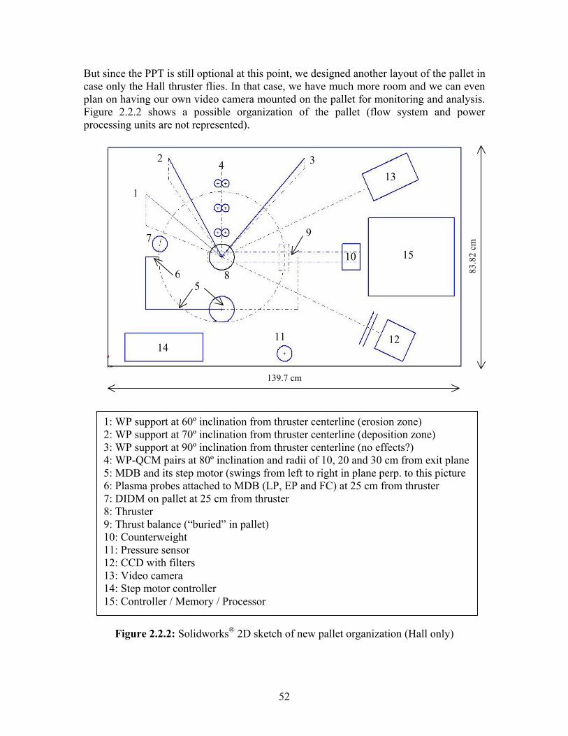
52

But since the PPT is still optional at this point, we designed another layout of the pallet in case only the Hall thruster flies. In that case, we have much more room and we can even plan on having our own video camera mounted on the pallet for monitoring and analysis. Figure 2.2.2 shows a possible organization of the pallet (flow system and power processing units are not represented).

Figure 2.2.2: Solidworks® 2D sketch of new pallet organization (Hall only)

139.7 cm

83.8

2 cm

1: WP support at 60º inclination from thruster centerline (erosion zone) 2: WP support at 70º inclination from thruster centerline (deposition zone) 3: WP support at 90º inclination from thruster centerline (no effects?) 4: WP-QCM pairs at 80º inclination and radii of 10, 20 and 30 cm from exit plane5: MDB and its step motor (swings from left to right in plane perp. to this picture6: Plasma probes attached to MDB (LP, EP and FC) at 25 cm from thruster 7: DIDM on pallet at 25 cm from thruster 8: Thruster 9: Thrust balance (“buried” in pallet) 10: Counterweight 11: Pressure sensor 12: CCD with filters 13: Video camera 14: Step motor controller 15: Controller / Memory / Processor

1

2 34

5 6

7

8

9

10

11 12

13

14

15

53

Here is a simplified 3D sketch of the reorganized pallet:

Figure 2.2.3: Solidworks® 3D sketch of new pallet organization (Hall only) Details on primary instruments (i.e. corresponding to the primary objectives)

Quartz Crystal Microbalances (QCM’s)

Position: The QCM’s would be used to measure the amount of depositions at a given angle from the thruster centerline. As explained in paragraph 1.1.2, the deposition zone is identified to be at angles between 70 and 80º from the thruster centerline. We chose to put them at 80º because it is a position where sensitive surfaces may be found when the thruster is integrated to a satellite, and also because by being in the expected deposition zone we should get a good measurable signal. Finally, we would put them at different distances from the thruster exit: 10, 20 and 30 cm.

Expected measurements: Expected deposition rate is 1.5x10-4 to 1.5x10-3 Å/sec,

and the resolution of QCM is commonly of the order of a monolayer of atoms. Status: We own 4 space qualified MK-16 QCM’s from QCM research, donated

by the AFRL. We would use 3 of them on the pallet and save the 4th one for ground testing and as a backup. Paragraph 3.2 explains the work done so far on QCM ground testing. One issue remaining for space flight is how to shutter them when we want to protect them from any contamination, and unshutter them when we want to do the measurements. Also, we need to design a casing enabling temperature control of the MK-16.

WP/QCM supports

DIDM

MDB

Video camera

CCD with filters Pressure sensor

Thruster andcounterweight

54

Witness Plates (WP’s)

Position and expected measurements: We would put one witness plate close to each of the 3 QCM’s (at 80º inclination from centerline) because the measurements of these two instruments are interesting to compare. Moreover, we would put other WP in each of the three zones defined in paragraph 1.1.2 and figure 2.2.2:

- Zone 1 at 60º from thruster centerline (the erosion zone is for angles <65º) - Zone 2 at 70º from thruster centerline (the deposition zone is between 70 and 80 º) - Zone 3 at 90º from thruster centerline (where we should not detect any effects).

The number of WP in each zone can be adjusted to test different distances, different materials, etc.

Status: Lockheed Martin has worked a lot on the WP technology but we need to adapt it for space flight. For example, like in the QCM case, we need to work on the shutter design.

Faraday Cup (FC)

Position: The FC is one of the instruments that are going to be installed on the MDB and swept through the plume at a radius of 25 cm (the MDB itself is detailed in paragraph 2.4). To limit the disturbance induced in the plasma, we design the FC so that it fits inside a 1-cm2 area.

Expected measurements: the current density at 25 cm is estimated to be j=0.1 to 5 mA/cm2, so the FC should be able to measure j=0.05 to 10 mA/cm2 with a resolution of 0.02 mA/cm2. Also we would bias the collecting plate negatively to reject 10 eV electrons, and use a positively biased grid to reject ions selectively.

Status: We will build this probe ourselves and take it thought the space qualification process. A first prototype has just been built and tested, as detailed in paragraph 3.3.

Quadruple Langmuir Probe (LP)

Position and expected measurements: The LP will also be installed on the MDB and swept through the plume. The expected electron densities are ne=4x10+14 to 2x10+16 m-3, the electron temperature Te = 2 to 5 eV.

Status: Quadruple Langmuir Probe design is done by Jurg Zwahlen from WPI. A

prototype was built; the status of this work as well as additional testing that we did in MIT are reported in paragraph 3.4.

Emissive probe (EP)

Position and expected measurements: The EP is the third of the 3 instruments mounted on the MDB. It is used to determine precisely the plasma potential and we expect a value close to Vp= 20 V.

55

Status: Yassir Azziz is working on this instrument in MIT (reference [36]). The design issues currently being tackled are the miniaturization on the probe (so that it does not disturb the plasma too much) and also heat transfer problems. A prototype should be built later this year.

Details on secondary instruments (i.e. corresponding to the secondary objectives)

Thrust balance

Position, measurements, resolution and status are discussed in a specific section of this chapter (paragraph 2.3).

Color video camera

Position: We would mount the video camera on the pallet, in a corner as far as possible from the thruster to have a better field of view. Also, as shown on figure 2.2.2, no instruments should be placed between the camera and the thruster: in particular, the position of the WP’s is studied so as not to hide a part of the plume from the camera.

Expected measurements: There are two goals to this video camera. First we would

download a “skeleton” of images (one every 10 seconds for example) to have a sort of real-time monitoring of the whole system (thruster, MDB movement…). Also, the complete “movie” would be used later on in the analysis to correlate the thrust and the presence of a central spike in the plume. Therefore, the camera does not need to be high speed but needs to have enough resolution to see the spike.

Status: As explained in paragraph 3.5, we tested the feasibility of this instrument and the relevance of the images by using a digital color video camera in the lab. We now need to find a camera that can be operated in space and if possible buy it off-the-shelf.

CCTV cameras These cameras are located in the corners of the Shuttle Payload Bay and can be used upon request by the customers who have experiments in the Payload Bay. The characteristics of these cameras are detailed in a NASA document referenced in Appendix B. We requested their use from NASA and we would use them to see the far field extension of the plume.

CCD with filters

Position and expected measurements: Similarly to the video camera we would place the CCD arrays and the filters in a corner of the pallet. The filters would enable us to take pictures of the plume at selected wavelengths corresponding to transitions for the Xenon atoms and ions. Therefore we would have a “map” of the plume that would enable us to understand better where the different species form.

56

Status: Ground testing started with narrowband filters and a digital camera as detailed in paragraph 3.5. Now we need to find space-qualified CCD arrays and filters, and to design an interface to hold them on the pallet and gather the “pictures”. Here are finally some details on environmental instruments:

Digital Ion Drift Meter (DIDM)

Position: The DIDM (figure 2.2.4) resolves incoming ions by energy and direction (its principle is roughly the same as a RPA). It would be mounted on the pallet at a radius of 25 cm from the thruster, close to where the MDB probes are located when the MDB is in its starting position as drawn on figure 2.2.2. Therefore we would be able to compare plasma parameters as measured by these different instruments.

Figure 2.2.4: DIDM Expected measurements: In the back plane, the expected densities are ne=0 to

2x10+14 m-3 (giving a current density of 0 to 60 µA/cm2, with a resolution of the order of 0.6 µA/cm2). Expected energies are 0 to 30 eV, which we will measure with a resolution of 1 eV.

Status: AFRL has confirmed they will lend us one of their DIDM instruments.

They are already space qualified and are designed to withstand the environment of unmanned launchers so they would work on the Shuttle. The only problem is with the aero-braking heat upon re-entry (DIDMs are very sensitive and could be “fried”). The latest version of AFRL DIDMs is called DIDM 3 and has improved capability of counting the ions; it can also store its own data and has a 422 bus interface.

Pressure sensor

Position and expected measurements: We expect the pressure to go down to 10-10 torr in the Shuttle wake, but to be mostly around 3x10-7 torr. We would like to use a commercial, off-the-shelf vacuum gauge.

57

Status: Two options were investigated so far. Varian, Inc. makes gauges with built in controllers like the Eyesys IMG (inverted magnetron gauges). They work like most cold cathode type gauge tubes: they consist of a central anode and a cylindrical cathode. A strong permanent magnet surrounds these elements. A DC voltage of about 2000 volts is applied to the positively charged anode to attract electrons. The magnetic field forces the electrons into helical paths to increase the possibility of electron-molecular collisions. The collisions produce ions. The positive gas ions are now attracted to the negatively charged cathode. The resulting ion current is measured and calibrated in units of pressure. This Varian IMG is pretty robust but not space qualified.

The company Kernco, Inc., on the other hand, makes space qualified gauges that

have already been used on the Space Shuttle as shown in figure 2.2.5. If one of those is present on the Shuttle during our mission, we may not need to have our own.

Figure 2.2.5: Kernco gauges Optional instruments are also being considered: Retarding Potential Analyzer (RPA)

It would be used only as a backup if finally we cannot have a DIDM. We would try to buy it off-the-shelf.

EMI The EMI experiment would consist of an antenna and a receiver placed on each side of the plume; we would then be able to check for any distortion or attenuation of a signal that would have gone across the plume.

All these instruments are now summarized in Table 2.2.1. Details on QCM, LP,

FC, video and filters ground testing are in chapter 3. Note that at this point, only the QCM’s and DIDM are flight-qualified models.

1. Vacuum Gauge Flown on Shuttle missions STS 46 (July 92) and STS75 (Feb. 96). 2. Bear Rocket - Pressure monitoring during orbital Particle BeamExperiment. 3. Space Shuttle Instrumentation - Gas Sampling System. Has flown andcontinues to fly on all Shuttle missions since Atlantis STS-71 (June 95).

58

Table 2.2.1: Summary of instruments 1: primary objectives, 2: secondary objectives, E: environmental instruments, B: backup.

Note that on the sketch of the pallet, Propellant Regulation System and Power Processing Unit are not shown. Development of these elements will probably be done at specialized companies. An example is given in McLean, C. H., et al., “Development of a Flight Propellant Regulation System for Hall Effect Thrusters”, IEPC 01-321.

2.3) Design of the thrust balance for flight

A graduate student in Draper Laboratory, Jareb Mirczak, is working on this design for his Master of Science Thesis “A Milli-Newton Thrust Stand for Space Shuttle Flights” (title as known as of March 20, 2000). We provided him with the following specifications: Range: Nominal thrust is 10.5 mN so measure from 0 to 25 mN. Precision required: 100 µN to be able to see if the spike is on or off. Time response: 2 sec. Dimensions:

Dimensions of pallet: 33.38 x 55.65 inches (0.8478 x 1.4135 m) Dimensions of thruster:

- Outer “apparent” diameter (including poles): 4 inches (10.16 cm) - Length 3.577 inches (3.772 with the center cone), or 9.034 (9.581) cm - From the Busek documentation, the envelope without cathode, cables and mounting brackets is 10 cm in diameter by 12 cm long - The thruster weighs about 1 kg, plus 0.2 kg for the cathode. The total should not 1.5 kg (3.307 lbs).

Desired Measurement

Instrument

Dep

ositi

on

Ero

sion

Ion

Den

sity

E

lect

ron

T

Plas

ma

Pote

ntia

l C

urre

nt

Den

sity

Thr

ust

Farf

ield

Pl

ume

Opt

ical

E

mis

sion

s T

hurs

ter

Puls

ing

EM

I

Pres

sure

Plas

ma

Bac

kgnd

QCM 1 B Witness Plates B 1 Langmuir (on MDB) 1 1 B B Emissive Probe (on MDB) 1 Faraday Cup (on MDB) 1 Thrust Balance 2 Shuttle Cameras (CCTV) 2 CCD with filters 2 Video camera 2 EMI 2 Vacuum E DIDM (or RPA) E

59

Constraints:

The concept must be able to function under microgravity conditions (for example, a design involving weights for calibration would be useless).

Vibrations, mechanical and structural resistance: the thrust balance has to sustain

vibrations and loads especially during take off and landing (see CARS section 3); structures must resist to a conservative 11 g’s in each axis. If possible the design should be insensitive to parasitic vibrations during operation.

Minimize weight and required power:

- Maximum weight for Hitchhiker DBP is 600 lb (272.155 kg) with center of gravity within the envelope (see CARS page 2-37); - Maximum simultaneous total customer power is 1600W (500W for a single customer), and the nominal maximum total customer energy is 10 kWh/day. - The source of power from Shuttle is two 28 V DC (+/- 4 V DC) 10 amps power lines.

Temperature range (CARS page 2-46) is around -76 to 65ºC. This depends on the

attitude of the Shuttle: Bay to Sun (hot), Bay to Earth (nominal), Bay to Space (cold). For double bay pallet mounting, GSFC will provide thermal model data on the HH plates and their attachments. Also, external surfaces of thruster are at a maximum of 200ºC.

Last but not least, safety of the astronauts and avoiding damages to the other

payload bay hardware should be a continuous concern along the design. For example, if the design involves moving parts, it has to be latched when not used, especially during lift-off and landing. A list of allowable materials is given in CARS Appendix B: data on materials (alloys) with high resistance to stress corrosion cracking (page B4) and materials with low outgassing and flammability data (page B7) are available.

Particular issues to be addressed:

Stress relief for Xenon lines and thruster power supply wires, so that they do not interfere with thrust measurements (the lines should be very flexible to add minimum stiffness). At the same time, we need to make sure they are strong enough to resist 11-g loads, which is one of the constraints quoted above.

The thrust balance has to be sensitive enough to measure a 10-mN thrust but the

user must also be able to distinguish this tiny thrust from the vibrations created by the environment. For example, we would need to ask Mission Control to provide us with the log of when exactly the Shuttle attitude thrusters fired so that we can subtract his thrust from our data. If possible we would require that the Shuttle thrusters be not fired during our thrust measurements.

60

Evacuation of heat from the thruster: about 100W of heat coming from the

thruster has to be evacuated, otherwise the thrust balance calibration would be changed.

Given these constraints and issues, the following designs were eliminated: - Inverted pendulum – problem with loads/vibrations, - Long-period pendulum – complex design, - Electromagnetic – problem with loads and fuel interface.

The current design choice is a torsional pendulum (figure 2.3.1). It has some

heritage with thrusters (PPT, micronewton, nanonewton, micronewton extended range thrust stand). The flexures are cylinders specially designed to respond to torsion but not to other stresses. Consequently, the thrust causes torsion in the flexures and very small displacements at the ends of the stiff boom that holds the thruster. This displacement would be measured by a sensor like a LVDT (Linear Variable Differential Transformer) or a fiber-optic based optical sensor. The thrust balance would also use active damping to get good time response, thanks to a damping coil located next to the sensor. Coil and sensor would be located under the counterweight, not on the thruster side of the balance, to avoid thermal problems. This design eliminates vibrations in the operating environment, sustains launch loads in all axes, and is not based on gravity. Cooling would be done either by conduction through the pallet or by radiation (we would “bury” the thrust balance in the pallet, see figure 2.3.1). More details will be available in Jareb Mirczak’s thesis (reference [37]).

Figure 2.3.1: Current status of the thrust balance concept (courtesy of J. Mirczak)

We also have a laboratory thrust balance (for use with ground experiments only)

based on the inverted pendulum concept. It is shown on figure 2.3.2 and uses a LVDT to measure the displacement of the platform on which the thruster is sitting, and another coil for active damping. We are currently using it to better understand the stress relief system, the electronics, the data acquisition principles and the thermal issues involved. For example, we are in the process of rebuilding the controller because the damping did not seem to work properly. A user interface was created with Labview and is described in Stephanie Thomas’ thesis (reference [38]).

Thrust balance “buried” in pallet. Underneath:

Damping and sensing coils Flexures

Counterweight

Stiff boom

Thruster

Underneath: Channel for radiative cooling

61

Future work on this lab thrust balance includes finishing the controller, verifying the Labview interface, calibration and data acquisition.

Figure 2.3.2: Laboratory thrust balance

2.4) Design of the mechanical arm

The mechanical arm or “Mechanical diagnostics boom” (MDB) is designed by Andrew Suryali from Worcester Polytechnic Institute. As this arm is intended to carry three instruments, scientific considerations were important. The requirements are:

- Ability to sweep the instruments through the plume at a given radius and in a

plane containing the centerline of the thruster - Ability to hold 3 different probes (and their wires) so that they are all in the same

plane and at the same radius, only at different angles from the centerline - Ability to achieve a positioning precision of 1º.

Mechanical considerations were also important. The design was done considering

two thrusters (the Hall and the PPT). The requirements are:

- Due to issues with robustness, it is preferable to have simple, 1-DOF motion - Any probe on the PPT side will need to be cleaned after several pulses. One

option for cleaning is to bring probe over to Hall side while Hall thruster is operating.

- Constraints due to the Shuttle (launch loads, safety…) are also applicable as seen in paragraph 2.3. For the required motions, two designs were possible: a “swinging” or a “rotating”

boom (as illustrated in figure 2.4.1):

Platform

To controller Damping coil

Xe inlet

Stress relief system for wires and fuel lines

LVDT

62

Figure 2.4.1: The two MDB concepts

The rotating option enables us to clean the PPT probes in the Hall plume. But it does not satisfy the requirement of a constant radius for the sweeps. So the final design was chosen after a compromise: a Two-Degree-of-Freedom twin-boom with two diagnostic arms welded 25 cm from boom base (figure 2.4.2). The T shape can rotate around the vertical part of the T, and swing around the base (therefore the diagnostics arms are swinging at a constant 25 cm radius from the thruster).

Figure 2.4.2: Swinging/Rotating concept The boom would be a hollow tube with internal space for wiring. Motion would

be controlled by stepper motors having the required precision and torque. In the case where only the Hall thruster flies (the PPT is still not confirmed at this point), we would need only the swinging motion, and only one side of the T. More details such as load analysis (boom must be able to withstand 11-g acceleration on each axis for Shuttle qualification) will be available in Andrew Suryali’s Master of Science thesis (reference [39]).

Swinging

Rotating

Swinging

Rotating

63

The 3 instruments to be swept are LP, emissive probe, and FC. We need to have them rather far away from each other, but at same radius from the thruster. Also, the device binding them together should have a minimal surface and be rather “open” to minimize the disturbance induced in the plasma and avoid “trapping” ions or neutrals. Future work consequently includes the design of the interface between the 3 probes and the MDB. A possible concept is shown in figure 2.4.3 (the MDB is swinging from left to right as indicated by the arrows).

Figure 2.4.3: Probes attachment concept

2.5) Operational Procedures

For flight experiments is it especially important to have a precise experimental protocol, because all operations have to be remotely controlled. So we started developing scenarios of how the experiments would be conducted, from the highest, most general point of view down to the precise sequence of operations. Here is the Sequence of operations - Highest level (global scenario of the experiment in flight):

1) Shuttle checkout phase: read background pressure (from pressure sensor) and plasma background (from DIDM instrument). Keep these sensors on during the whole experiment.

2) Turn cameras (CCD, video and CCTV) ON 3) Calibrate the thrust balance; acquire data continuously when the thruster is on 4) Unlatch the MDB 5) Run the thruster at the desired operating point 6) Move the arm to the desired acquisition point 7) Read data from instruments on arm (FC, LP, emissive probe). If available, read

also from RPA (Retarding Potential Analyzer) and EMI instruments. 8) Do it again from step 6 until all plume is swept (increments of 1º) 9) Change operating point and do the sweep again (i.e. restart from step 5) 10) When all operating points have been investigated, re-latch arm, stop thruster, stop

acquisition of thrust data, lock thrust balance (in that order).

Radii of 25 cm

Attachment to MDB

Probes

Thruster exit

Swinging motion

64

A part of the experiment (plasma parameters) is then completed. One sweep represents 180 acquisition points, so if we stay 5 seconds at each point to allow the arm and plasma to settle it takes 15 minutes. We will investigate a maximum of 10 operating points (which makes 150 minutes), and we need to wait several minutes between different operating points to allow the thruster to reach steady state operation, which makes a total of about 3 hours. Then we go on with the deposition/erosion experiments.

11) Unshutter the deposition and erosion instruments (QCM, witness plates), start data acquisition.

12) Run the thruster at nominal operating point for longest period available (1 day) 13) Shut down the thruster 14) Re-shutter deposition and erosion instruments 15) Turn cameras OFF.

If EMI experiments are available they could take place during that one-day

operation of the thruster. Once this general protocol is established, we need to go down to the precise sequence of commands that the onboard processor will have to transmit to the hardware. Turning on the thruster, for example, involves a complex start-up sequence that needs careful controller design. Therefore, we would use a sequenced command methodology: it does not require real-time commanding from the ground, but changes in the sequence can be uploaded from time to time if needed. The controller launches the execution of a task and then moves on to a new task when specified variables reach specified values, as described for example in a GRAFCET diagram.

In this kind of diagram, boxes represent the actions that the processor commands to the hardware. Between boxes, a test called a transition is specified, for example “variable A has the value x”. It means that the controller will go on to the next action (box) only when the transition is “TRUE”. A temporization can be introduced by the notation t/“step at which we need the system to wait”/“time we want to wait” (for example, t/2/60 means “wait 60 minutes at step 2”). Two parallel horizontal lines represent the case where there is an alternative: if a transition A is true, then action X happens, but if B is true, action B happens. Several GRAFCETs can be done in parallel for multitasking. Finally, some of the tasks in boxes can actually refer to another GRAFCET (if they are complex and require several actions). So there are also several levels in GRAFCETs. Several GRAFCETs were made for the thruster operation: Cathode first start, Cathode subsequent starts, Thruster first start, Thruster nominal start, Thruster and cathode shut down.

Only the first one is presented here (figure 2.5.1). The others can be seen in Appendix C2 and serve as an operating manual for the thruster.

65

Figure 2.5.1: GRAFCET of the first cathode run sequence of operations Now more GRAFCETs need to be done to detail MDB operation, data acquisition from the various instruments, etc. In particular, timing issues are important and must be specified (cf on figure 2.5.1 between steps 2 and 3). For example, we would use the following sequence for the MDB: move MDB to desired acquisition point; wait 5 seconds for arm and plasma to settle; keep MDB at this position for 10 seconds and read data from the probes; then write the data in the memory while the MDB is moving to the next operating point. All these diagrams will be very useful when it comes to developing the software that will command the whole experiment, as detailed in the next paragraph.

Keeper current = 0A

Increase keeper voltage to 75 V

Turn off heater

Keeper current around 0.7A, voltage around 20V

Cathode standby mode; Go tothruster operation diagram

6

7

8

Heater current = 0

Heater current = 6.5 A, voltage ~ 6.5 V

Open Xe tank

Turn on heater power supply

Startup configuration: all valves shut, cathode cold, thruster off, power supplies off.

Start command received

0

1

2

3

4

5

In current controlled mode, increase current by 0.5A every ½ hour, starting at 2A (5 hours total)

Keep heater current at 6.5A andturn on keeper power supply

Cathode flowmeter ON @ 1 sccm . t/2/60 min (Wait for lines to fill up 60 minutes)

Xe tank open

Heater power supply ON @ 0V, 0A

Keeper power supply ON @ 0V, 0A

7’ Set keeper voltageback to 0V andincrease cathode flowto 2 sccm (if already,go to manual control)

K = 0V, cm& = 2 sccm

Open cathode flowmeter @ 1 sccm

66

2.6) Software engineering For this part we have the help of Professor Charles Coleman from SERL (Software Engineering Research Laboratory) and undergraduate student Nida Farid. The system-level role of the software is the following:

- Thruster start up sequence (includes turning on PPU and flow system) - MDB operation - Data collection, on-board processing and storage of the data, downloading when

possible - Specifically for the deposition and erosion instruments (QCM and witness plates):

remove covers before operation and replace them afterwards.

The SERL uses an application developed by Safeware Engineering Corporation, SpecTRM (pronounced "spectrum": Specification Tools and Requirements Methodology), to support the development of safe systems and software. As described on this company’s web site, SpecTRM features intent specifications, a type of specification method built upon systems theory and cognitive engineering (i.e., a combination of ideas from systems engineering, cognitive psychology and human factors). More precisely, intent specifications are written by considering successively 5 levels in a means-ends hierarchy, as detailed in a paper by MIT Software Engineering Professor Nancy Leveson (reference [40]).An example of this can be found in the Sample TCAS Intent Specifications (Traffic Alert and Collision Avoidance System, reference [41]). Each level provides intents (“why”) to the level below it, and high-level system requirements and constraints are therefore traceable down to code and vice-versa. LEVEL 1: SYSTEM PURPOSE: no design decisions at this point.

System goals Design constraints: normal, or safety-related Assumptions Limitations Design evaluation criteria and priorities Results of analyses for system level qualities

LEVEL 2: SYSTEM DESIGN PRINCIPLES: basic scientific and engineering principles needed to achieve the behavior specified in the top level. LEVEL 3: BLACKBOX BEHAVIOR MODEL

While levels 1 and 2 are usually paragraphs familiar to systems and safety engineers and written in English, level 3 is more familiar to software engineers. The blackbox behavior model specifies the system components and interfaces including the human operators. Also, it includes an environment description (assumed behavior of the external components).

67

Each component of the system corresponds to a “box” in which the different modes of the component are detailed. For example for the MDB (figure 2.6.1):

Figure 2.6.1: MDB blackbox

Around each component box we place inputs, outputs, relationships between components, and timing specifications. We then build state machines that enable us to see how the component goes from one state to the other (similarly to the transitions in GRAFCET representation). To do these state machines, SpecTRM uses the executable requirements specification language SpecTRM-RL (RL stands for Requirements Language).

Then, a set of input values is written in an input file, and fed to the state machines. According to the defined transitions, the state of each component will evolve. A graphical visualization shows the state of the system during execution. Execution speed is variable, and the simulator can be single-stepped to examine system behavior in detail. Finally outputs are recorded for examination after the execution, and this enables us to check that no combination of inputs can put the system in an undesired or even dangerous state.

The great strength of SpectRM-RL is that requirements specifications are also executable models, so as we just saw, system behavior can be simulated directly from the requirements and the engineers can check that safety is ensured. Finally the two bottom-levels of the intent specification concern implementation of this model into code: LEVEL 4: PHYSICAL AND LOGICAL FUNCTION: usual software design documents. LEVEL 5: PHYSICAL REALIZATION: software itself (code), instructions for use, training of the users, maintenance requirements.

As we are just beginning to address the software engineering issue, Nida Farid’s work is currently to:

- Write down the system-level requirements in a paragraph in English (Level 1); - Learn what the safety constraints are for Shuttle payloads software (Level 1); - Input (1) and (2) into SpecTRM and deduce design principles (Level 2); - Create the blackbox model and run simulations (Level 3).

MDB

Moving

Stopped

Unknown

68

Step 1 is completed (figure 2.6.2) and we are currently working on step 2. Before implementation in SpecTRM of these high-level requirements we will also need to organize them better (following the example of the TCAS Intent Specifications from reference [41]) and particularly refine the timing specifications.

Figure 2.6.2: Project goals paragraph

Note that we “start the thruster for 1 hour at 5 sccm” then “restart it at the nominal operating point” because this is how the thruster start-up procedure must be done according to the Busek BHT-200 operating manual.

In our case, as mentioned in paragraph 2.1, Hitchhiker provides the customers

with a transparent data system so that the software used for ground testing would be directly transferable to flight operations. So we will from the beginning design the software according to space flight security and autonomy constraints. It is indeed important to limit the cost of correcting errors at a later step by building required system properties into the design from the beginning rather than emphasizing assessment at the end of the development process when effective response is limited and costly.

Initialize the Shuttle checkout phase. Read and record the data from the pressure sensor for thebackground pressure, and the DIDM instrument for the plasma background. Turn the camerason. Unlock and calibrate the thrust balance. Acquire the value of the thrust continuously fromthis point on. Unlatch the rotating arm. Start the thruster and run it for one hour with the Xeflow set at 5 sccm for surface conditioning in the thruster channel. Then restart the thrusterand run it at the nominal operating point of 7 sccm. Move the rotating arm to the firstacquisition point. Read and record the data from the Faraday Cup, Langmuir Probe andEmissive Probe, which are located on the rotating arm. If the Retarding Potential Analyzer(RPA) and the EMI instruments are available, also read and record the data from them. Movethe arm to the next acquisition point. Read the data from the various probes and instruments asdetailed before. In a similar way move the rotating arm in sequence to the various desiredacquisition points, and take the data at those points. Repeat this until the entire plume has beenswept. Now, change the thruster operating point. Bring the rotating arm back to its startingposition, and start the entire procedure of data acquisition at the desired positions as explainedearlier. Repeat this process for the remaining operating points. When all the operating pointshave been investigated, re-latch the arm. Then, stop the thruster. Next, stop acquisition of thethrust data (from the thrust balance) and lock the thrust balance. Now, start the next phase ofthe experiment. Unshutter the deposition and erosion instruments (QCM’s and witness plates).Start data acquisition using these instruments. Run the thruster at the nominal operating pointfor the longest available period, if possible 1 day. Continue the data acquisition from theinstruments for this entire period. At the end of this period, shutter the deposition and erosioninstruments, then shut down the thruster.

69

Chapter 3

Ground Testing at the MIT Space Propulsion Laboratory

Theory is when it works and you don’t know why. Practice is when it doesn’t work and you know why.

Here we achieve both: it doesn’t work and we don’t know why… - A desperate scientist

This last chapter deals with the work I did in the MIT Space Propulsion

Laboratory on the design of instruments for the space experiment. The setup in the lab will be presented first; then details will be given on the QCM, Faraday Cup, Langmuir Probe (primary objectives) and optical diagnostics (secondary objective).

3.1) Set up in the MIT chamber The MIT Space Propulsion Laboratory owns a small vacuum chamber (about 1.5 m in diameter and 2 m in length). Pumping is done by a mechanical pump for roughing, then by two cryopumps (OB-400 and CT-10) to achieve Ultra-High Vacuum (the design pumping speed is 7000 l/sec for Xenon).

Pressure is monitored by a thermocouple gauge for the range above 10-3 torr, and by a cold cathode gauge that can measure pressures down to 10-9 torr. Both are controlled by a Varian Multi Gauge Controller. When there is no Xenon flow in the chamber, the pressure is below the range of the hot filament probe so we take the “base pressure” Pb to be negligible. When Xenon is flowing in the chamber, we need to correct the indicated pressure Pi to take into account that the pressure sensors are calibrated for nitrogen, not Xenon:

87.287.2PiPPPP b

bicorrected ≈+−=

70

The pumping speed is such that when a Xenon flow of 8 sccm is established in the thruster (7 sccm in the thruster itself and 1 sccm in the cathode), the corrected pressure is of the order of 2x10-5 torr. This corresponds to about 6750 l/s, which agrees with the design pumping speed. Figure 3.1.1 is a picture of the chamber.

Figure 3.1.1: MIT Space Propulsion Laboratory’s vacuum chamber The chamber has 5 electrical feedthroughs and 6 fluids feedthroughs, respectively in yellow and in blue on figure 3.1.2:

Figure 3.1.2: Vacuum chamber ports

QCMStep motorcontroller Thruster

Probe on arm

Window

Thruster Xenon

Cathode Xenon

Water for target

“Target” coatedwith graphitepaint and water-cooled to protectthe wall.

Water for thrustbalance cooling

Single Langmuir Probe (stationary)

71

The thruster we used for the tests is the Busek BHT-200 Hall thruster (figure 3.1.3); it is an older version of the Tandem-200 presented in introduction but has the same characteristics. It was installed on the top of a two-shelved “bridge” so that the centerline of the thruster coincides as exactly as possible with the center of the chamber.

Figure 3.1.3: Busek BHT-200

The pictures in figure 3.1.4 give a good idea of the effects of erosion and depositions of this thruster after an estimated total of 40 h of operation. On the left, erosion has happened on the part of the cathode that is closer to the channel exit. On the right, depositions occurred on the opposite side.

Figure 3.1.4: Erosion and deposition

The power supplies for the thruster are installed in a rack and consist of: - Kepco 10V-10A power supply for the heater (H) and magnet (M) - Sorensen DCS300-3.5E (300V-3.5A) power supply for the keeper (K) - Sorensen DCS600-1.7E (600V-1.7A) power supply for the discharge (D)

The flow system consists of a 25L Xenon tank and two Omega Engineering flow meters (1 to 10 sccm). Power supplies and flow system are shown in figure 3.1.5.

Nominal Operating Conditions: Thruster Mass Flow Rate: 0.7 mg/sec Cathode Mass Flow Rate: 0.1 mg/sec Discharge Voltage and Current: 300V, 0.65A Magnet Voltage and Current: 1.67V, 0.39A Thrust: 10.5 mN ISP: 1530 sec Total Efficiency: 35%

Cathode

Central coneand annuluschannel exit

Top shelf ofthe “bridge”

72

Figure 3.1.5: Power supplies and flow system

Finally, the bottom shelf of the bridge was used to support a mechanical arm, so that we could sweep instruments through the plume. The arm itself was made of Bosch T-slotted extrusion: it is aluminum to keep the weight low but it does not bend thanks to its special cross-section. The arm is composed of a long horizontal piece and a vertical crosspiece (figure 3.1.6). Brackets are used to hold the different parts of the structure in place. Untightening the brackets allows the parts to slide in each other.

Figure 3.1.6: Bosch T-slotted extrusion and our sweeping arm

The motor used to make the arm turn is Model #5609M (6.0V, 1.2A) from The Motion Group, Inc. It comes with a SID 2.0™ Step Motion System (controller and program in Basic to pilot the motor). Details on the arm operation are given in Appendix C in the form of a manual and figure 3.1.7 shows the arm installed in the chamber. As in most articles and papers where moving probes were used, the probe lies in the horizontal plane containing the centerline of the thruster, and the position of the probe is given by the angle θ in degrees from the centerline (positive on the right, negative on the left).

Adjustable counterweight

Connector to motor shaft

Adjustable radius

Instrument holder

Adjustableheight

73

Figure 3.1.7: Bridge, arm and thruster in the chamber; Probe positioning (top view)

3.2) QCM

Characteristics

Four MK-16 CQCM’s from QCM research were donated by the AFRL to the MIT Space Propulsion Laboratory (figure 3.2.1).

Figure 3.2.1: MK-16 CQCM

Two identical crystals are used (sense and reference) in a crystal pack (made of

gold plated Oxygen Free High Conductivity copper), which is supported from the base by four heat-isolating struts. As explained in chapter 1, the crystal frequency varies with temperature as well as mass deposition, but by placing the two crystals at the same temperature these effects cancel out. The crystal pack is well insulated from the base, so that the case can be held at less than 10 K while the crystals are heated, by means of a heater (25 W wirewound precision resistor using at most 1.6 W of power), to any desired temperature. This allows the investigator to raise the temperature of the crystals from 10 K up to 400 K, measure the mass change rate as a function of the sense temperature and deduce by QCM thermogravimetric analysis (QTGA) the sensor surface deposition

Centerline

θArm

Probe

Thruster

Plume

Enlargement

Sense crystal

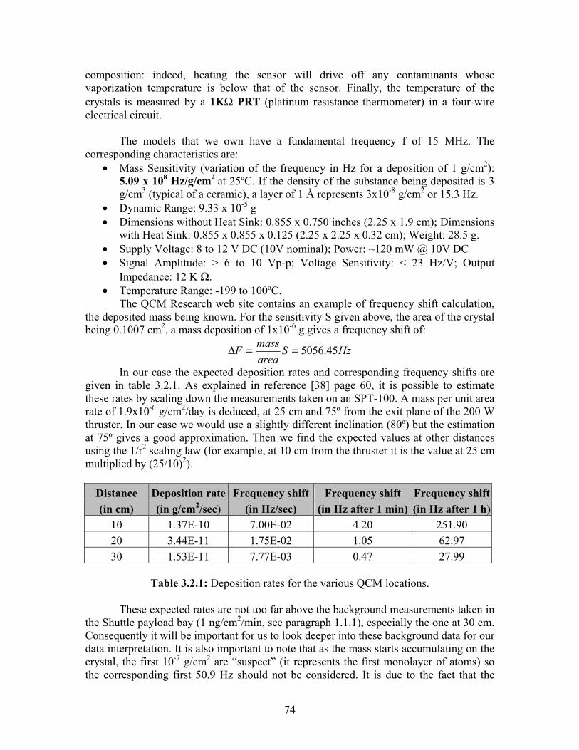
74

composition: indeed, heating the sensor will drive off any contaminants whose vaporization temperature is below that of the sensor. Finally, the temperature of the crystals is measured by a 1KΩ PRT (platinum resistance thermometer) in a four-wire electrical circuit. The models that we own have a fundamental frequency f of 15 MHz. The corresponding characteristics are:

• Mass Sensitivity (variation of the frequency in Hz for a deposition of 1 g/cm2): 5.09 x 108 Hz/g/cm2 at 25ºC. If the density of the substance being deposited is 3 g/cm3 (typical of a ceramic), a layer of 1 Å represents 3x10-8 g/cm2 or 15.3 Hz.

• Dynamic Range: 9.33 x 10-5 g • Dimensions without Heat Sink: 0.855 x 0.750 inches (2.25 x 1.9 cm); Dimensions

with Heat Sink: 0.855 x 0.855 x 0.125 (2.25 x 2.25 x 0.32 cm); Weight: 28.5 g. • Supply Voltage: 8 to 12 V DC (10V nominal); Power: ~120 mW @ 10V DC • Signal Amplitude: > 6 to 10 Vp-p; Voltage Sensitivity: < 23 Hz/V; Output

Impedance: 12 K Ω. • Temperature Range: -199 to 100ºC.

The QCM Research web site contains an example of frequency shift calculation, the deposited mass being known. For the sensitivity S given above, the area of the crystal being 0.1007 cm2, a mass deposition of 1x10-6 g gives a frequency shift of:

HzSareamassF 45.5056==∆

In our case the expected deposition rates and corresponding frequency shifts are given in table 3.2.1. As explained in reference [38] page 60, it is possible to estimate these rates by scaling down the measurements taken on an SPT-100. A mass per unit area rate of 1.9x10-6 g/cm2/day is deduced, at 25 cm and 75º from the exit plane of the 200 W thruster. In our case we would use a slightly different inclination (80º) but the estimation at 75º gives a good approximation. Then we find the expected values at other distances using the 1/r2 scaling law (for example, at 10 cm from the thruster it is the value at 25 cm multiplied by (25/10)2).

Distance Deposition rate Frequency shift Frequency shift Frequency shift(in cm) (in g/cm2/sec) (in Hz/sec) (in Hz after 1 min) (in Hz after 1 h)

10 1.37E-10 7.00E-02 4.20 251.90 20 3.44E-11 1.75E-02 1.05 62.97 30 1.53E-11 7.77E-03 0.47 27.99

Table 3.2.1: Deposition rates for the various QCM locations.

These expected rates are not too far above the background measurements taken in the Shuttle payload bay (1 ng/cm2/min, see paragraph 1.1.1), especially the one at 30 cm. Consequently it will be important for us to look deeper into these background data for our data interpretation. It is also important to note that as the mass starts accumulating on the crystal, the first 10-7 g/cm2 are “suspect” (it represents the first monolayer of atoms) so the corresponding first 50.9 Hz should not be considered. It is due to the fact that the

75

sensitivity of the instrument is attained only after a certain amount of mass has deposited. Finally the detectability of the signal is about 1.9x10-4 Hz/min so our predicted rates are well in the range.

QCM Research makes fully Space Flight Qualified CQCM’s which have flown in several different configurations. It may be interesting for us to acquire the Flight Electronics Unit (FEU), which can control and collect data from independent QCM’s. Documentation on this unit includes vibration (both random and sinusoidal), shock, hard radiation exposure, solar thermal radiation, acoustical wave transmission, EMC and thermal cycling. The read-out rate and interface are to be designed by the customer. MK-16 QCM’s in particular have flown on several missions. The Canadian Space Agency (CSA) placed two of them on the End Effector (hand) of the Remote Manipulator System (Shuttle arm) on-board Shuttle Flight STS-52 and several follow-on flights. The QCM’s had a layer of material placed on the surface that was sensitive to the presence of atomic oxygen (O) so that the highly reducing atmosphere would, in effect, etch off the deposited material and cause the beat frequency to decrease. When CSA determined that they had finished with the experiment, NASA Johnson then directed the astronauts to explore the region that the arm could reach for contamination. In 1995, on a follow-on flight (STS-74), the same configuration was used when the shuttle positioned itself close to the Russian attitude control and reboost thrusters on the MIR Space Station to have the QCM’s detect both transient and persistent surface contamination. NASA is continuing to use the QCM’s on the arm to measure erosion rates by atomic oxygen in their Space Shuttle flights.

Installation in the laboratory Only one of the four QCM’s we own would be used for ground tests in order to keep the three others unspoilt for the space experiment itself.

Support: In the chamber we would like to mount the QCM at an angle of 80º from the thruster centerline (same position as the one planned for the space experiment). Therefore, we are thinking of mounting the QCM on a square bracket (figure 3.2.2); these brackets can in turn be conveniently screwed on the bottom shelf of the bridge or on the grid that constitutes the “floor” of the chamber.

Figure 3.2.2: Bracket for QCM support

76

The issue that remains for laboratory installation is temperature control. As a matter of fact, unlike the MK-10 (which is a TQCM), the MK-16 does not have built-in thermoelectric heat pumps (based on Peltier effect). In our case, we will consequently need to cool the QCM with an outside mechanism (passive cooling). The temperature should be stabilized at a value close to that of the nearby surfaces: indeed, the goal of the QCM is to measure the depositions at a specific location, so the sensors conditions should be as similar as possible to those of the surfaces around it. Then, thanks to the built-in heater, we can perform the QTGA as explained before. Connections: Our QCM’s have ten 32" Constantan Pigtail wires coming out of them, and they are labeled as shown on figure 3.2.3:

Figure 3.2.3: MK-16 QCM wires Note that T1 (cathode) and T2 (anode) actually consist of two wires bundled

together (this is for the temperature sensor). Consequently, only 8 connections are required. These wires must be connected to the 9-pin end of a cable referenced as M2010, as shown on figure 3.2.4:

Figure 3.2.4: QCM-to-cable connection (view of the QCM side from the cable side)

H+ Heater power H- Heater ground SIG, or ∆f Beat frequency V+ Oscill. voltage T1 Cathode T2 Anode COM Common ground CG Case ground

QCM case

77

Finally, the other side of the cable is a 15-pin D-sub connector and can be directly plugged in the backpanel of the controller (see below). It is important to use this cable because its shielding is especially designed to ensure less noise in the signal.

Laboratory controller: The controller provided with the four MK-16 is a M2000 (figure 3.2.5). It communicates with the host computer over an industry standard RS232 serial link. In our configuration it controls four CQCM’s at once through four 9-pin connectors on the back panel. The controller sends data at a rate of one reading per second per channel. It accommodates temperature sensors and drives the heaters. While autonomously controlling the temperature, both temperature and frequency data for each channel are sent to the host over the serial link.

Figure 3.2.5: M2000 laboratory controller As explained in the M2000 manual, the temperature data sent to the host is

given in degrees Kelvin, with the least significant digit representing 0.01 K. The electronics add no more than a 0.25 K error to the accuracy of the sensor for absolute accuracy. For relative accuracy, which eliminates thermal drift, the added error is less than 0.1 K. Frequency data sent to the host is given in Hertz. The relative accuracy is better than one part per million. For all frequencies (1 KHz to 600 KHz), data is sent in the form of seven digits with a floating decimal point. Thus, for a frequency of 100 KHz, the least significant digit represents 1/10 Hz (0.1 Hz).

Collimator: For the space experiment, we expect the thruster to be the only source of contamination. But in the vacuum chamber, particles could also come from sputtering from the walls of the chamber. Consequently, we are building a collimator in order to reduce the field of view of the QCM so that only materials from the thruster are deposited (see figure 3.2.6).

78

Figure 3.2.6: Ground test setup (not to scale) Rigorously speaking, on the figure above, the continuous lines define a zone called “umbra” and the dashed lines the “penumbra”. For simplicity we considered only the dashed lines for the design. This collimator would be used only for ground tests, not in space. Requirements are:

- Use a material that is very resistant to sputtering so that depositions cannot come from the collimator itself;

- Ensure that the aperture is big enough for the sense crystal to still see the whole exit plane of the thruster;

- Have holes on the sides of the collimator so that no pressure build-up can occur from the gases that enter the collimator. These holes should be protected so that particles can exit but not enter the collimator through them.

The design currently being constructed is shown on figure 3.2.7 (Solidworks® drawing).

Figure 3.2.7: QCM collimator (oblique and side views)

Other issues and design for flight

Since the QCM’s themselves are already space-qualified, only a few issues remain for the flight diagnostics package design:

Thruster centerline

Thruster Lines-of-sight

QCM

Collimator

7 cm

Attachment to QCM

Pressure-relief holes and

protective “skirt”

79

- Heat transfer calculations for temperature control: as explained earlier, we want to monitor contamination on surfaces near the thruster, so the QCM sensors should reproduce these surfaces as precisely as possible: same temperature, same electric potential, same surface conditions for incoming molecules. Therefore we need to control the temperature of the sensor so that it is the same as that of the surfaces;

- Evaluation of the effect of insolation (sun-radiation) on the measurements; - Design of a shutter for the QCM’s when not in use: to avoid the use of motors,

active materials (Smart Memory Alloys) may be a idea to consider; - Command and data handling: a QCM Research Flight Controller that can handle

4 QCM’s costs about $180000. If our funding is not enough, we may have to handle controller design as part of the experiment data collection design.

3.3) Faraday cups/RPA

Goals and characteristics

We want to use a Faraday Cup to measure directed flux in the 200W Hall thruster plume. More precisely, we want a measurement of the current density at a constant radius of 25 cm from the exit plane, from –90º to +90º with respect to the centerline. Requirements for the design are the following:

- We want to miniaturize the FC as much as possible: it is important first for the

precision of the measurement, because 1 cm at 25 cm from the exit plane represents 1.146º. Moreover, this is an intrusive measurement technique, so the smaller the FC, the less disturbance to the plasma. Consequently the whole FC “head” should fit in a surface of approximately 1-cm2.

- We want to detect selectively scattered ions and CEX ions: scattered ions come

from elastic collisions; they have a high energy (about half of the initial accelerating energy, so 100 to 200 eV) while CEX ions have low energies (20 to 30 eV).

From a plasma collisions model, the scattered ions distribution should be

maximum at 45º from the centerline, and the CEX ions for angles around 90º. The ratio of their quantities (scattered over CEX) should be the ratio of their cross sections (1/3 to 1/2). We would like to check this ratio as well as the location of high energy scattered ions to make sure the usual 45º canting of thrusters in satellites is enough to prevent those ions to hit the satellite (they may be more damaging than the CEX even if there are fewer of them).

80

Design and building instructions

The concept we chose was that of a classic FC with a guard ring (shield) around a collector plate (biased negatively to collect ions, not electrons). We added a positively biased grid in front to repel ions selectively (according to their energy).

The collector plate: In reference [38], initial calculations were made to determine what range of collected current we should expect (page 65). As the mechanical arm sweeps through the plume, the current density (conservative) range is about 0.1 to 5 mA/cm2. We also want to collect a current that is big enough to be measurable by usual laboratory equipment. Measuring a 10 µA current seems feasible and this leads to a minimum collector plate dimension of 3 mm in diameter. Note that 3 mm at 25 cm represent 0.687º, which meets one of our requirements.

We decided to use eV parts from Kimball Physics, Inc. They are standard parts

made from high temperature materials and high purity insulators and are especially intended for use in high vacuum. Here are the steps to follow for the construction.

The collector plate is consequently 3.175 mm in diameter (0.125’). The rod enables us both to apply the bias to the collector and to measure the current in a circuit (at the end of the rod opposite to the plate).

We take the following eV parts: SS-RP-B125: round plate, Ø 0.125’ SS-RO-B-6000: stainless steel rod We spotweld them together.

To make the guard ring we use: Al2O3-TU-4000: alumina tube SS-LR-C: stainless steel lock ring SS-PL-B3x3: square plate with 3x3 holes (side is 0.400’ or 1.016 cm, so the area is 1.032 cm2) SS-WR-250/031: wire ring SS-CY-250/250: cylinder (Ø 0.250’x 0.250’) Al2O3-SP-C-250: alumina spacer We enlarge the center hole of the square plate so that the alumina tube can fit in it.

81

See also figure 3.3.2 for the overall arrangement of the FC “head”. Finally we introduce the stainless steel rod in the alumina tube; the round plate comes to rest on the alumina tube end, so that the cylinder, alumina spacer and round plate form a flat surface. The stainless steel rod is prevented from sliding inside the alumina tube thanks to a screw clamp SS-SC-B2M. The resulting assembly is shown in figure 3.3.1.

Figure 3.3.1: Assembly without grid and close up on the “head”

The grid: For the ions to “see” the positively biased grid, we need the wires of the grid to be spaced so that the sheath around them covers the interspaces. The sheath size is larger than the Debye length λd by a factor of (Vbias/Te)¾ (~ 7 for a 30V bias) and

e

e

e

ed n

TenkT 025.692

0 == ελ .

Reference [38] page 63 shows a Debye length plot for angles of –90 to +90º at 25

cm from the thruster exit (i.e. exactly where we want to operate). λd is between 0.2 and 1 mm. It is 0.6 mm at 45º i.e. where we expect scattering to be maximal; so between 2 wires, the ions “feel” the bias if the interspace is less than 1.2 mm, keeping the factor of 7 as a “safety factor”. The wires themselves have a diameter of 5 mils (0.13 mm). For practicality of realization as well as to avoid having too many wires, and consequently too much impingement of the wires themselves, we chose a spacing of about 1 mm. Here is the explanation of the construction:

Then we assemble everything (in this order): - Spotweld the wire ring on the cylinder - Spotweld the wire ring on the square plate - Slide the alumina tube in the center hole of

the plate, use the lock ring to hold it so that it stays just a little bit under the cylinder edges

- Spotweld the lock ring at the back of the plate

- Slide the spacer between the cylinder and the alumina tube.

SS rod

Screw Clamp

Alumina tube

Square plate and cylinder

Head fits in ~ 1 cm2

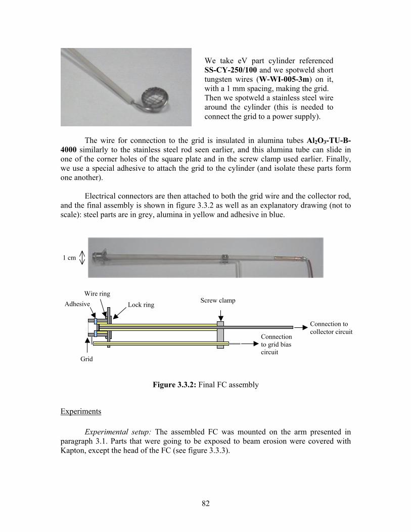
82

The wire for connection to the grid is insulated in alumina tubes Al2O3-TU-B-4000 similarly to the stainless steel rod seen earlier, and this alumina tube can slide in one of the corner holes of the square plate and in the screw clamp used earlier. Finally, we use a special adhesive to attach the grid to the cylinder (and isolate these parts form one another).

Electrical connectors are then attached to both the grid wire and the collector rod,

and the final assembly is shown in figure 3.3.2 as well as an explanatory drawing (not to scale): steel parts are in grey, alumina in yellow and adhesive in blue.

Figure 3.3.2: Final FC assembly

Experiments

Experimental setup: The assembled FC was mounted on the arm presented in paragraph 3.1. Parts that were going to be exposed to beam erosion were covered with Kapton, except the head of the FC (see figure 3.3.3).

We take eV part cylinder referenced SS-CY-250/100 and we spotweld short tungsten wires (W-WI-005-3m) on it, with a 1 mm spacing, making the grid. Then we spotweld a stainless steel wire around the cylinder (this is needed to connect the grid to a power supply).

Wire ring

Lock ring Screw clamp

Grid

Connection to grid bias circuit

Connection to collector circuit

1 cm

Adhesive

83

Figure 3.3.3: Faraday Cup on the arm in the vacuum chamber The circuitry involved is shown on figure 3.3.4. The biases are provided by a 2-

channel TENMA laboratory DC power supply. The grid will be biased to +30 V because this is the limit of the power supply, and it is enough to repel low energy CEX ions. The collector will be biased to –12 V with respect to the tank (since the plasma is at a potential of the order of 10 volts above the tank, this should be enough to repel electrons). In order not to cause too great a disturbance in the plasma, the guard ring is left floating.

Figure 3.3.4: FC circuitry Before any experiment, we verify that the different parts are well isolated from

each other: the grid is isolated from the guard ring by the adhesive, the collector by the alumina, etc. To determine the collected current, we measure the voltage across the resistor in mV with a laboratory voltmeter and we divide by R. The voltmeter has an internal resistance of 10 MΩ and averages the values it is getting, so even if the data is a bit noisy, we can still read an average value.

Protocol: After the probe is installed in the chamber and electrical connections checked, the chamber is leak-tested, then pumped down overnight. The following day the thruster is started and the following measurements are taken.

Grid

+ 30 V

R=4.64 kΩ

- 12 V

Ground (same astank wall)

Col

lect

or V

Arm covered with Kapton

Faraday Cup

84

- Preliminary experiment: Just after the thruster is started for the first time, the flow is 5 sccm. We do a first sweep from –90º to the centerline (in steps of 5º or 2º in the interesting regions), with the collector biased to –12 V and the grid not biased. Then we redo the same sweep, but with the grid biased to +30 V;

- “Real” experiment: We restart the thruster with its nominal flow of 7.12 sccm.

We check that when the thruster is not on, the voltmeter measures 0 V, so there is no collected current. This time, we sweep again from –90º to the centerline, but at each point we read the collected current with AND without the grid biased.

Results: Curves of collected current were obtained. During the “real” experiment,

the pressure in the chamber was 2.9x10-5 torr (corrected for Xenon) and the thruster parameters were: Discharge voltage/current: 300 V / 0.9 A

Keeper voltage/current: 6 V / 0.2 A Heater voltage/current: 4 V / 3 A Magnet voltage/current: 1.9 V / 0.4 A

The measurements themselves lasted about 1 h, and the thruster operated for 3h30 total. The total flow of Xenon in cathode and thruster was 0.8 mg/sec, which represents 0.53 L/hour at ordinary temperature and pressure conditions. The pressure in the Xenon tank dropped accordingly by 30 psi. Figure 3.3.5 shows the current density curves (both in normal and in logarithmic axes). We plotted only one side of the centerline (the other one is assumed symmetric).

Ion current density(7.1 sccm, P=2.9x10-5)

0.00E+00

5.00E-01

1.00E+00

1.50E+00

2.00E+00

2.50E+00

3.00E+00

-90

-80

-70

-60

-50

-40

-30

-20

-10 0

Angle from centerline

Cur

rent

den

sity

(mA

/cm

2 )

unbiased gridbiased gridscaled data

(a)

85

Ion current density(7.1 sccm, P=2.9x10-5)

1.00E-03

1.00E-02

1.00E-01

1.00E+00

1.00E+01-9

0

-80

-70

-60

-50

-40

-30

-20

-10

0

Angle from centerlineC

urre

nt d

ensi

ty (m

A/c

m2 )

unbiased gridbiased gridscaled data

(b)

Figure 3.3.5: Current density curves (a, normal plot; b, log plot) The black dashes on the curves at each data point are error bars. They were

calculated by taking into account: - The precision of the voltmeter (±1 mV), which introduces an constant error of

2.72x10-3 mA/cm2 in the current density; - The precision to which the collector area is known: the diameter of the round

plate is guaranteed by the manufacturer of eV parts to be 0.125 inch, but to be conservative, we assume the precision is ±0.001 inch. This introduces an error of ±1.6% when calculating the current density. In this evaluation we also assume that the whole area of the collector is collecting ions, i.e. we do not take into account edge effects.

Another source of error is the error in angle from the arm positioning (±1º) but it is small and is therefore not shown on the graphs.

The shape of the curves in figure 3.3.5 seems to agree with usual plume current

density profiles. We plotted in yellow the values obtained by scaling down the SPT-100 data reported in reference [38], figure 2.7. The data is first scaled as the inverse square of distance (25 cm in our experiment versus 1 m in the SPT-100 experiment), then with thruster power (200W versus 1350W). The factor to go from SPT data to our data is consequently .37.21350

20025.01

2 =× At large angles, the discrepancy can be explained because better vacuum was achieved for the SPT-100 test than for ours. At small angles, we see that in order to get a good agreement we should still apply a correcting factor to the scaled data. The yellow curve would then shift down.

86

Before analyzing the curves more precisely it is important to note that measurements between –13º and the centerline were hard to obtain: for each new position, the voltmeter would show a first value (the one we recorded), then increase gradually (about 1 mV/second). In some cases the increase seemed to continue for several minutes, in other cases, the voltage then suddenly dropped. This may be due to the fact that this region is where the beam is the most intense, so charges could be building up on the surfaces, especially on the insulators, thus altering the behavior of the probe. As a matter of fact, we noted also that the grid power supply was drawing a current of + 0.1 A, indicating that electrons were collected. Also, as seen on the Faraday Cup drawing, some insulating parts are exposed to an intense flux of particles. In particular, the alumina spacer inside the guard ring is in a region where the plasma is not neutral because of the collector bias. In the eV parts manual it is recommended to avoid this situation because it decreases the resistance of the insulator. Since the measurement shows a gradual increase, it is more likely to be due to a thermal issue or to the degradation of some material, than to charging interactions. The adhesive we used seems to be the weakest part and may be eroded away. Consequently, it will be necessary to check the probe for damage, and to make the necessary design changes subsequently.

Now let us study the influence of the grid. With a biased grid we should collect

less current especially in the regions where low energy CEX ions are a majority (i.e. large angles) because only the ions above 50 eV hit the collector. This is verified on the graphs in figure 3.3.5. However, the preliminary experiment (with 5 sccm flow) did not show this pattern. This may be due to the fact that the current from the plasma was too small to overcome the bias in the collector circuit, thus making the measurements doubtful. Indeed, for very large angles (> 70º), the measured voltage was negative.

As for the detection of the scattered ions around 45º, our grid bias of +30V could

not repel them. The curves do not show much difference between the biased and the unbiased case. However, a close-up of the –60º to -40º region in figure 3.3.6 shows that below 53º the FC with the biased grid collects less current than the unbiased one, indicating that some low energy ions are repelled. Above that angle, there is not much difference between biased and unbiased measurements (the biased measurement is above the unbiased one between about –53º to –15º, but since the error bars overlap, this difference is not significant). Finally, the biased grid seems to repel a significant portion (20-30%) of the ions for small angles (-15 to 0º). Because of the difficulty we had in taking the data there, more experiments are needed. But in case this trend is confirmed, a possible explanation is that there may be some low energy ions in this main beam region, due to background neutrals being ionized, double ions, or maybe products from the central “spike” of the plume (see details on the spike in paragraph 3.5).

87

Ion current density(7.1 sccm, P=2.9x10-5)

5.00E-02

6.00E-02

7.00E-02

8.00E-02

9.00E-02

1.00E-01

1.10E-01

1.20E-01

1.30E-01

1.40E-01

1.50E-01

-60

-58

-56

-54

-52

-50

-48

-46

-44

-42

-40

Angle from centerline

Cur

rent

den

sity

(mA

/cm

2 )

unbiased gridbiased grid

Figure 3.3.6: Zoom on the –60º to –40º region

We also compared this experimental data to simulations conducted by Shannon Cheng (reference [42], page 100: current density with the influence of background pressure). The comparison is shown on figure 3.3.7. The agreement is good for angles below 40º, but the code is known to underestimate the presence of ions at large angles, which is verified here.

Comparison with simulations

1.00E-02

1.00E-01

1.00E+00

1.00E+01

-90

-80

-70

-60

-50

-40

-30

-20

-10

0

Angle from centerline

curr

ent d

ensi

ty (m

A/c

m2)

s imulationsunbiased gridbiased grid

Figure 3.3.7: Measured and simulated data

88

Lastly, we calculated the beam current, which is the integral of the current density over a hemisphere at the chosen radius (25 cm). The formula is, with j the current density and r = 25 cm:

∫=2/

0

2 )sin(2)(π

ϑθπθ drjIB

Since we only have discrete values for j, we can evaluate this integral by the method of rectangles. The lower evaluation (i.e, with rectangles under the curve) gives 480 mA (53% of the discharge current of 900 mA); the upper evaluation (with rectangles above the curve) gives 578 mA (64% of the discharge current).

In an attempt to refine these calculations we tried to find an analytical fit for j by using the usual Lorentzian function:

)(100)(2

21

02

2

aaa

rj

++=

θθ

where r is the radius in cm, and θ the angle from the centerline. The unknown coefficients are determined by three particular values of j and θ chosen along the curve:

1st fit: with points θ = -90º, -45º and -5º we find )31.116

45.161009.8(16)( 24

++×−= −

θθj .

2nd fit: with points q = -50º, -20º and –9º we find )31.116

45.161009.8(16)( 24

++×−= −

θθj .

Figure 3.3.8 shows a plot of these fits. The first one is more accurate at large

angles, the second one at small angles. The corresponding beam currents are 562 mA (62% of the discharge current) and 498 mA (55%) respectively.

Ion current density(7.1 sccm, P=2.9x10-5)

0.00E+00

2.00E-01

4.00E-01

6.00E-01

8.00E-01

1.00E+00

1.20E+00

1.40E+00

1.60E+00

1.80E+00

2.00E+00

-90

-80

-70

-60

-50

-40

-30

-20

-10 0

Angle from centerline

Cur

rent

den

sity

(mA

/cm

2)

unbiased gridbiased gridLorentzian fit 1Lorentzian fit 2

Figure 3.3.8: Lorentzian fits

89

So finally we have a beam current around 60% of the discharge current. When evaluating the thruster efficiency, several processes must be taken into account: the beam current (fraction of the discharge current that goes in the plume, directly linked to performance), but also ionization utilization fraction in the discharge chamber, etc. The total efficiency of the BHT-200 is said to be 35%. We would consequently expect a higher (around 75-80%) beam current fraction, because of all the losses than need to be subtracted from the beam current to go down to this efficiency. For example, in reference [14] page 93, M. Fife uses a “beam energy efficiency” of 88% for a SPT-70. But our 60% is a first estimate and more experiments should be done before drawing conclusions. For instance, a better evaluation of the current density at small angles could change this amount: it is at small angles that the current density is bigger and thus contributes more to the beam current. Complementary experiments: On a second day of data taking, we used the same protocol as in the experiments described above (without a “preliminary experiment”), except we biased the collector more in order to make sure electrons do not hit the collector. We used the same circuitry but with a bias of –20V. Also, we did the sweep from 0º to +90º instead of –90º to 0º. The results are shown in figure 3.3.9 (blue curves), with a comparison with the measurements for a collector bias of –12V (red curves).

0.00E+00

5.00E-01

1.00E+00

1.50E+00

2.00E+00

2.50E+00

3.00E+00

3.50E+00

4.00E+00

4.50E+00

Angle f rom c e nt e r line

0.00E+00

5.00E-01

1.00E+00

1.50E+00

2.00E+00

2.50E+00

3.00E+00

3.50E+00

4.00E+00

4.50E+00

Angle f rom c e nt e r line

1.00E-02

1.00E-01

1.00E+00

1.00E+01

Angle f rom c e nt e r line

1.00E-02

1.00E-01

1.00E+00

1.00E+01

Angle f rom c e nt e r line

Figure 3.3.9: Influence of the collector bias on ion current density Top: normal plots; Bottom: log plots

90

We see that the –20V bias gives a much higher current density, although the thruster parameters and pressure where the same as when we took the data with a –12 V bias. Actually, this high current density does not make sense because beam current calculations give values above 4 A for IB while the discharge current is only of the order of 0.9 A! Possible explanations are that the probe may have been damaged during the first experiments, as explained earlier, or that a higher collector bias disturbs the plasma and changes the amount of ions being collected (i.e., a –20 V bias attracts more ions than would normally hit the collector). More experiments are needed to determine how exactly the collected current depends on the collector bias.

Finally, our last experiment concerned the influence of pressure. The ultra-high vacuum is obtained with two cryopumps, so we do not have many means to change the pressure, but we compared the case where the two pumps are pumping to the case where one of them (the CT-10) was shut down. The results are shown in figure 3.3.10.

0.00E+001.00E+002.00E+003.00E+004.00E+005.00E+006.00E+007.00E+008.00E+009.00E+001.00E+01

0 10 20 30 40 50 60 70 80 90

Angle from centerline

Cur

rent

den

sity

(mA

/cm2 )

2.86E-5 torr4.48E-5 torr

Figure 3.3.10: Influence of pressure on ion current density When the two cryopumps were pumping, the pressure was 2.86x10-5 torr and the discharge current was 0.9 A. Without the CT-10, the pressure was about 60% higher (4.48x10-5 torr) and the discharge current was 1.07 A. The current density is much higher (2.4 times higher at small angles, 1.3 times higher at large angles) when the pressure is high. Again, on that day the probe may have been damaged from previous experiment so the absolute values are not certain (the values of IB are again higher than the discharge current, which does not make sense). But the observed trend should be confirmed by doing more experiments.

91

Other issues and design for flight More experiments need to be carried out in the lab. In particular:

- To address the problem of the gradually increasing current at small angles, it would be useful to rebuild a similar FC but without the grid and therefore without the adhesive. Also it may be a good idea to use a shorter alumina spacer, or no alumina spacer at all, so that no insulator is exposed to direct particle flux. Testing this new FC should provide answers to the problem as well as check for the repeatability of the measurements;

- It is also important to check if the collector bias has a big influence on the

measurements (as suggested by the comparison between –12V and –20V biases). This can be done by biasing the new FC to intermediate voltages (between –20 and 12V);

- For the influence of pressure, again complementary data should be taken with

the new FC to confirm the observed trend. Intermediate pressure levels (between 2.85 and 4.48x10-5 torr) may be achieved by putting grids on the pumps openings in the chamber, so that the pumping speed is reduced but not as much as when we shut down one of the pumps completely;

- We need to address more precisely the noise issue. For example, instead of

measuring a voltage across a resistor to deduce the current, we could amplify the current through an operational amplifier (“op amp”);

- Then, influence of thruster parameters (flow, discharge voltage…) on the

magnitude of the current density could be investigated. Also, different radii could be tried (for example do a sweep at 60 cm and check we are still getting an acceptable beam current);

- Finally, it would be interesting to work more on the influence of the grid: try

higher biases; try making smaller interspaces, etc.

On the design for flight side, the main characteristics of the FC developed here can be reused. Only the structure needs to be strengthened to meet space qualification criteria. Command and data handling involves only biasing some parts and measuring a current.

92

3.4) Langmuir probes

Goals and characteristics

Jurg Zwahlen from WPI is taking care of the Quadruple Langmuir Probe (QLP) design and results interpretation (reference [43]) for the ETEEV experiment, and it is a whole Master of Science thesis in itself. Therefore, we focused on finding the influence of some parameters on the measurements rather than taking extensive data.

This study will consequently address the following issues:

- Comparison of the data taken with the lab-made QLP to that of a commercial Single Langmuir Probe (SLP), and especially verification of the repeatability of the measurements;

- Evaluation of the interference between two probes that are close to one another; - Influence of the orientation of the probe tip with respect to the flow; - Influence of some key thruster parameters (mass flow rate, discharge voltage)

on the SLP measurements.

A description of the two probes follow. Figure 3.4.1 shows the Single Langmuir Probe (called “ESPion”) bought from Hiden Analytical with its controller and software. Upon first installation it is calibrated using an internal resistor. The tip of the probe is a 10 mm long nickel wire and is 0.15 mm in diameter. The probe is attached to a flange so that it can be mounted on one of the vacuum chamber feedthroughs. A linear Z-motion device exists for this probe but we did not purchase that option; consequently, the SLP is stationary. The collected current is transmitted to the controller via a coaxial cable and the controller is in turn connected to a computer by a serial link.

Figure 3.4.1: Commercial Langmuir Probe

The QLP we used is similar to the one used by Jurg Zwahlen as shown on figure 3.4.2. This probe is intended to be mounted on the arm and swept through the plume (it is not stationary). It is composed of an alumina tube in which there are 4 holes. Tungsten wire is slid in each of the holes and a part of the tungsten is left out of the tube, creating

93

the probe tips. The tungsten wire we used is 15 mils (0.38 mm) in diameter, and the tips are 350 mils (8.89 mm) long.

Figure 3.4.2: Lab made QLP (with a dime to indicate scale) What made our experiments different from Zwahlen’s is that:

- We did not apply any bias to the wires: traditional QLP operation requires biasing the wires with respect to one another, but here we did not connect them to any power supply. Consequently it is actually floating Single Langmuir Probes, not really a Quadruple Langmuir Probe;

- We did not keep three of the wires aligned while the fourth one was bent perpendicularly to the others, as commonly done for QLP measurements. Instead, we used a special tip arrangement (as shown in figure 3.4.3) to see the influence of the orientation on the measurements.

Figure 3.4.3: Special tip arrangement and numbering (#4 is coming out of the page)

1

4 2

3

Probe tips

4 tungsten wires isolated from each other by heat shrink

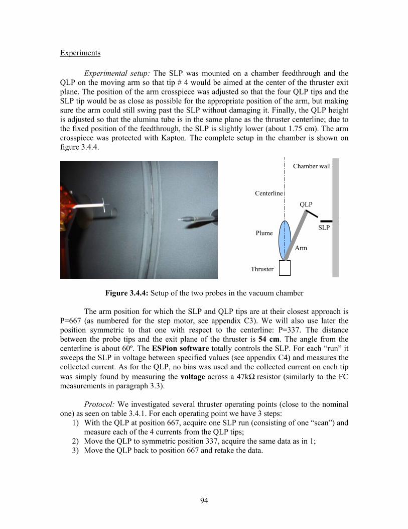
94

Experiments

Experimental setup: The SLP was mounted on a chamber feedthrough and the QLP on the moving arm so that tip # 4 would be aimed at the center of the thruster exit plane. The position of the arm crosspiece was adjusted so that the four QLP tips and the SLP tip would be as close as possible for the appropriate position of the arm, but making sure the arm could still swing past the SLP without damaging it. Finally, the QLP height is adjusted so that the alumina tube is in the same plane as the thruster centerline; due to the fixed position of the feedthrough, the SLP is slightly lower (about 1.75 cm). The arm crosspiece was protected with Kapton. The complete setup in the chamber is shown on figure 3.4.4.

Figure 3.4.4: Setup of the two probes in the vacuum chamber

The arm position for which the SLP and QLP tips are at their closest approach is P=667 (as numbered for the step motor, see appendix C3). We will also use later the position symmetric to that one with respect to the centerline: P=337. The distance between the probe tips and the exit plane of the thruster is 54 cm. The angle from the centerline is about 60º. The ESPion software totally controls the SLP. For each “run” it sweeps the SLP in voltage between specified values (see appendix C4) and measures the collected current. As for the QLP, no bias was used and the collected current on each tip was simply found by measuring the voltage across a 47kΩ resistor (similarly to the FC measurements in paragraph 3.3).

Protocol: We investigated several thruster operating points (close to the nominal one) as seen on table 3.4.1. For each operating point we have 3 steps:

1) With the QLP at position 667, acquire one SLP run (consisting of one “scan”) and measure each of the 4 currents from the QLP tips;

2) Move the QLP to symmetric position 337, acquire the same data as in 1; 3) Move the QLP back to position 667 and retake the data.

Centerline

Arm

QLP

Thruster

Plume

Chamber wall

SLP

95

Consequently, with step 1 we can compare SLP and QLP data. But what is more, by comparing 1 and 3 we can check for repeatability of the measurements; and by comparing 1 and 2 we can check for plume dissymmetry and interference of the probes on one another (in 1 they are close, in 2 they are far). Moreover, the ESPion software can be used to do automatic analyses of the SLP runs and deduce plasma parameters (Te, ne, ni, Vf, Vp) for the different thruster operating points.

Test # P (correc) thruster

mg/s D voltage Comments, observations START

0 out 0 0 In vacuum 1 6.21E-06 0 0 only cathode (just after warm up)3 2.10E-05 0.5 300 5 sccm

RESTART 5 3.00E-05 0.7 300 NOMINAL

OBJECTIVE 1 8 2.69E-05 0.6 300 9 2.83E-05 0.65 300 11 3.17E-05 0.75 300 12 3.38E-05 0.8 300

OBJECTIVE 2 20 2.97E-05 0.7 325 21 2.97E-05 0.7 350 24 2.97E-05 0.7 275 25 3.00E-05 0.7 250

Table 3.4.1: Thruster operating points for Langmuir Probes experiment.

Test 0 is a control. 1 and 3 are taken during the start up sequence of the thruster and test 5 is the nominal operating point. Objective 1 is to see the influence of the thruster flow; objective 2 is to see the influence of the discharge voltage. Finally, before shutting down the thruster at the end of the experiment, we swept the QLP from –90º to the centerline. The thruster was at its nominal operating point.

Results: We will first address the comparison between SLP and QLP data. It should be noted however that Langmuir Probe measurements are known to be good only to 10-20%. The comparison was conducted with the thruster at its nominal operating point. We compared the absolute values of the current we obtained on the unbiased QLP tips to the current collected by the SLP when the bias was 0 V. Since the SLP and QLP probe tips do not have the same area by construction, we divided the measured currents by the tip areas and compared the current densities. The data we obtained is shown on figure 3.4.5.

Investigation of the influence of thruster parameters

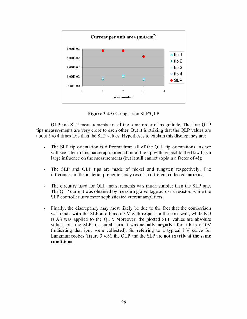
96

Current per unit area (mA/cm2)

0.00E+00

1.00E-02

2.00E-02

3.00E-02

4.00E-02

0 1 2 3 4

scan number

tip 1tip 2tip 3tip 4SLP

Figure 3.4.5: Comparison SLP/QLP

QLP and SLP measurements are of the same order of magnitude. The four QLP tips measurements are very close to each other. But it is striking that the QLP values are about 3 to 4 times less than the SLP values. Hypotheses to explain this discrepancy are:

- The SLP tip orientation is different from all of the QLP tip orientations. As we

will see later in this paragraph, orientation of the tip with respect to the flow has a large influence on the measurements (but it still cannot explain a factor of 4!);

- The SLP and QLP tips are made of nickel and tungsten respectively. The

differences in the material properties may result in different collected currents;

- The circuitry used for QLP measurements was much simpler than the SLP one. The QLP current was obtained by measuring a voltage across a resistor, while the SLP controller uses more sophisticated current amplifiers;

- Finally, the discrepancy may most likely be due to the fact that the comparison

was made with the SLP at a bias of 0V with respect to the tank wall, while NO BIAS was applied to the QLP. Moreover, the plotted SLP values are absolute values, but the SLP measured current was actually negative for a bias of 0V (indicating that ions were collected). So referring to a typical I-V curve for Langmuir probes (figure 3.4.6), the QLP and the SLP are not exactly at the same conditions.

97

I-V curve for nominal point

-5.00E-06

0.00E+00

5.00E-06

1.00E-05

1.50E-05

2.00E-05

-5 -4 -3 -2 -1 0 1 2 3 4 5

Voltage in V

Cur

rent

in A

Figure 3.4.6: Conditions at which the comparison was made

The comparison is made difficult by the fact that the probes are in a zone close to the cut-off point, i.e. where the transition region begins and where the current is very sensitive to the voltage bias: below the cut-off point, the current is negative and rather “flat” (ion saturation region); above the cut-off point, the current increases quickly. Consequently, the comparison should be re-done, insuring that QLP and SLP are really at the same conditions and either at very negative or very positive biases.

Repeatability: Even if the SLP and QLP measurements agreed only to the order of magnitude, comparing measurements of steps 1 and 3 proved a good repeatability: as seen on figure 3.4.5, the measurements on each tip are the same for steps 1 and 3 (i.e. when the position is the same) within 10-20%.

Interference between probes: If the QLP and the SLP were interfering with each

other, the measurements of the SLP in steps 1 and 2 would be different: it has not moved, so the only thing that changed in the presence or absence of the QLP in the neighborhood. Figure 3.4.5 shows that the SLP values in 1 and 2 are exactly the same. The value in step 3 is slightly lower but still within 20%. So we concluded there was no noticeable interference.

This is confirmed by the fact that the probes are spaced by about 1 cm while the

Debye length in this region is of the order of: 4

20 107025.69 −×≈==

e

e

e

ed n

TenkTελ m

SLP condition (wall potential)

Floating potential

QLP condition?

98

with Te=1 eV=11600 K and ne=1014 m-3. Consequently the sheaths around the probes do not interfere with each other. Moreover, this shows no “draining” of the local plasma by either probe.

A last remark is that by comparing steps 1 and 2 on the QLP data, we see slightly higher values for step 2. Contrary to the SLP (which is stationary), the QLP has moved between 1 and 2, so this difference is probably due to a small dissymmetry of the plume or a small error in the probe placement (the positions in 1 and 2 are intended to be symmetrical with respect to the centerline).

Influence of orientation: In our case, the plasma is flowing, which makes the

analysis of the data more difficult than for most Langmuir Probe measurements, as explained in Chapter 1. The influence of the flow direction is well seen on figure 3.4.7. From our special tip arrangement we know that tip 4 is pointed at the thruster while tips 1, 2 and 3 are perpendicular to this direction. Consequently, tips 1, 2 and 3 present their “side” to the flow (thus collecting more current), while tip 4 presents only its “face”. The difference is very noticeable for angles from -30º to 0º because it is the region where the flux is very directed (at large angles, the direction of the flow is more “random”).

QLP sweep

0.00E+00

1.00E-03

2.00E-03

3.00E-03

4.00E-03

5.00E-03

6.00E-03

7.00E-03

8.00E-03

9.00E-03

-80 -60 -40 -20 0

Angle from centerline

Col

lect

ed c

urre

nt (m

A)

tip 1tip 2tip 3tip 4

Figure 3.4.7: Comparison between the QLP tips Influence of thruster parameters on SLP measurements: Until now all the analysis

we have done was with measurements at the nominal operating point of the thruster. Now we will investigate deeper other operating points thanks to the ESPion software automatic analysis capability.

The SLP raw data is I-V curves. In the automatic analysis, the floating potential

Vf is found first by fitting a second order polynomial around the point at which the

99

current is zero. Then, a first approximate for the plasma potential Vp is found by locating the point at which the first derivative maximizes. At this point three regions can be identified (ion saturation region < Vf, electron saturation region > Vp, transition region in between). A better estimate of the plasma potential is then found by fitting a straight line to the last two of these three regions, and taking the intersection of these lines. The electron temperature is found because the fit in the transition region is such

thatekT

edV

Id ≈ln .

Finally the program uses a user defined “probe area” to deduce electron and ion

densities. This implies that the user calculates beforehand the applicable collection area, using the model that is the most relevant for the plasma being investigated. In our case, since the SLP is really on the far side of the plume, we used 4.7 mm2 (the total area of the probe tip) for the automatic analysis. But this is a source of error since the flow, even on the edge of the plume, may be fairly directional, although it is hard to say in what direction. For the ion-collection side, the software uses Orbital Motion Limit (OML) theory. The automatic analysis performed for the selected operating points gave the results seen in table 3.4.2. Due to difficulties in finding fits, some of the values could not be found and are denoted by a “?”.

Conditions Vf (V) Vp (V) Te (eV) ne (m-3) ni (m-3)

nominal 1.34 5.88 0.87 4.08E+14 2.35E+15 flow 0.6 0.96 ? ? ? 1.98E+15 flow 0.65 ? 4.73 ? 2.07E+15 ? flow 0.75 0.596 5.25 0.896 4.79E+14 2.15E+15 flow 0.8 ? 5.17 ? 1.95E+15 ? DV 325 1 5.31 ? 2.46E+15 ? DV 350 0.953 ? ? ? 2.25E+15 DV 275 0.875 5.3 0.94 5.14E+14 2.42E+15 DV 250 1.05 ? ? ? 2.38E+15

Table 3.4.2: Results of automatic SLP analysis

The floating potential, plasma potential and electron temperatures do not seem to

be affected by the thruster parameters variations. The average values are 0.96 V, 5.27 V and 0.9 eV respectively. The electron and ion densities are of more interest. First, the order of magnitude (1014 to 1015) agrees well with the expectations in reference [38] page 59. For the operating points where both ne and ni could be calculated, we see that there is an important discrepancy between the two densities. This does not sound right because the quasi-neutrality of the plasma (ne = ni) should be verified over distances of millimeters. There is probably a problem in the data reduction done by the SLP software. In particular, as explained earlier, the software assumes the total area of the probe collects ions and electrons, which is a very crude approximation. By verifying “manually” some

100

of the values, we deduced that the values of ne could be trusted, while finding ni would require a more accurate model: OML theory may not be the best choice in our case, and the fact that the plasma is flowing may also be playing a role.

Since we cannot really get more information from so few numbers, let us investigate the influence of thruster parameters on the I-V curves themselves. First, figure 3.4.8 presents the influence of the thruster flow.

-1.00E-04

0.00E+00

1.00E-04

2.00E-04

3.00E-04

4.00E-04

5.00E-04

6.00E-04

7.00E-04

8.00E-04-5

0

-40

-30

-20

-10 0 10 20 30 40 50

Voltage bias (V)

Col

lect

ed c

urre

nt (A

)

flow 0.6 mg/sflow 0.65 mg/snominal (0.7)flow 0.75 mg/sflow 0.8 mg/s

Figure 3.4.8: I-V curves for different thruster flows

As expected, the higher the flow, the higher the collected current (except for the nominal case, which seems a bit too low: this may be due to the fact that the nominal data was taken before all others, so the conditions may have drifted during the interval of time).

It should be noted, however, that pressure in the chamber increases with the flow.

So the increase in collected current may also be due to a higher background pressure (and an increase in charge exchange). As charge exchange varies like the square of the flow, we plotted the collected current at a given bias (chosen to be 50V) versus the square of the flow on figure 3.4.9: it seems that the points can be fitted to a straight line that goes through the origin (in blue), which confirms increased charge exchange plays a role in the increase of collected current with thruster flow rate. The line represented here was found by taking the fourth data point (0.563; 7.06x10-4) as an anchor point and then finding the line that goes through this point and the origin.

101

Figure 3.4.9: Current increase at a given bias Finally, figure 3.4.10 is an attempt to see the influence of the discharge voltage (D. V.) on the measurements, but no clear trend could be deduced.

-1.00E-04

0.00E+00

1.00E-04

2.00E-04

3.00E-04

4.00E-04

5.00E-04

6.00E-04

7.00E-04

8.00E-04

-50

-40

-30

-20

-10 0 10 20 30 40 50

Voltage bias (V)

Col

lect

ed c

urre

nt (A

)

D.V. 250 VD.V. 275 Vnominal (300V)D.V. 325 VD.V. 350 V

Figure 3.4.10: I-V curves for different discharge voltages (D. V.)

4.00E-04

4.50E-04

5.00E-04

5.50E-04

6.00E-04

6.50E-04

7.00E-04

7.50E-04

8.00E-04

0.30

0.35

0.40

0.45

0.50

0.55

0.60

0.65

0.70

(flow)2

curr

ent f

or a

50V

bia

s

102

Other issues and design for flight Important future work on the Langmuir Probe include:

- Re-doing the comparison between QLP and SLP further from the cut-off point, for instance more towards negative biases (ion saturation region) and/or towards positive biases (electron saturation region), and ensuring that they are biased to the same potential;

- Developing an appropriate model for analysis (following for example Fife’s work

in reference [14]);

- Making a stronger packaging for flight qualification purposes (particularly the attachment to the MDB);

- Adapting the complicated Quadruple Langmuir Probe circuitry (different biases,

etc) for flight, work on the data acquisition and detail the flight specifications as for power and data rates.

In a last paragraph, we will now detail preliminary testing that we did for the proposed optical diagnostics.

103

3.5) Optical diagnostics

Goals and design

Optical diagnostics are among our secondary objectives. As explained in chapter 2, on the Shuttle we would use:

- The Shuttle CCTV cameras to see the expansion and shape of the far field plume; - A video camera aimed at the thruster to monitor the operation and especially

check for the presence of the “spike” (and correlate that with the thrust data, if available);

- A CCD with selected filters to map the optical emissions.

We do not have any flight design for these last two diagnostics, but we checked that the results they give are relevant. We are particularly interested in checking the impact of the spike on thrust. It is indeed a still unexplained phenomenon: it consists of a bright region right on the thruster centerline just after the exit plane. It is NOT in front of the channel from which the flow of ions comes from! A possible explanation could come from the flow profile at the exit of the channel, as seen on figure 3.5.1. This figure was reported in reference [5] from another paper (Gavrushin, V., Kim, V., “On influence of magnetic field characteristics in the parameters of ion flow at exit of accelerator with closed electron drift and extended acceleration zone”, Zurnal Teknicheskoy Fiziki, Vol. 52, #4, 1981). Some of the flow is seen to actually go towards the centerline. Since it is an axis of symmetry, flow comes there similarly on the other side. Consequently, collisions may occur there more than elsewhere, with emission of visible radiations.

Figure 3.5.1: Measurements of the flow at thruster exit

But this traditional explanation is not satisfactory. Indeed, simulations actually show a bigger concentration of ions there than elsewhere in the plume, but it is much more diffuse than what the observer can see with the naked eye. Effects other than just

104

density enhancement probably account for the spike shapes as seen further on figures 3.5.2 and 3.5.3.

Experiments in lab: We first used a Sony digital color video camera and recorded

about 20 minutes of thruster operation on a Fujifilm MiniDV cassette. This is very flexible because we can then convert the “movie” to usual digital movie formats.

The camera was started as the cathode was in its standby mode. The following

phases were observed with the frame-by-frame visualization (1 frame every 0.01 second, times in minutes : seconds : 1/100 seconds). The indicated pressure in the chamber was about 6x10-5, so 2.1x10-5 corrected for Xenon.

01:28:16 – The discharge starts. The plume is purple and spherical. As discharge current is increased, the plume becomes “shorter”, less spherical.

03:12:21 – We turn on the electromagnet, the plume becomes blue, which indicates the presence of ionized Xenon. As we increase magnet current and discharge voltage, the plume shape changes, as if the brighter part was concentrating more and more within a semi-sphere in front of the thruster exit.

03:31:07 – As we continue to increase the magnet current and discharge voltage, all other parameters remaining equal, the spike appears!

After 05:00:00 – The plume starts flickering. During that time we were increasing

the magnet current. At some point the plume becomes smaller and then disappears. As we start the thruster a second time, we observe the same kind of start up sequence, then a succession of changes in the shape of the spike. It seems that the “flickering” of the plume is actually due to this succession of changes. As we go through the movie frame by frame, we see that each frame is alternatively one of the following:

15:40:00 and 16:01:00 – “Trumpet” type of spike like in figure 3.5.2 (it becomes

larger as it goes farther from the thruster exit):

Figure 3.5.2: Trumpet spike

105

16:09:24 and 16:56:08 – “Needle” type of spike like in figure 3.5.3:

Figure 3.5.3: Needle spike This phenomenon is very fast. Frames are taken at a rate of 1 every 0.01 second

so the frequency is at least 100 Hz. At the same time the discharge current is fluctuating a lot, so these instabilities may be due to the power supply system.

We see from this short movie that a video camera provides valuable qualitative

information that can be used for monitoring purposes during the experiment (provided we can download the images from the Shuttle “real-time”) as well as for correlation with other measurements later on.

Finally, we tested the possibility of optical emissions analysis by taking pictures of the thruster at different operating points with a Canon PowerShot S-100 digital camera in front of which we placed different narrowband filters. The following set-up was used (figure 3.5.4):

Figure 3.5.4: Setup for optical diagnostics We chose to use Oriel narrowband filters. They are characterized by their central

wavelength λ (±2.0 nm); their bandwidth is 10 nm (±2.5 nm) and their transmittance around 50%. They are designed to operate from –50ºC to + 80ºC, and intermittently to 100ºC, while the rate of temperature change should not exceed 10ºC/minute. It should also be noticed that increasing temperature increases the central wavelength, almost

Camera

Thruster and plume

Chamber window

Filter

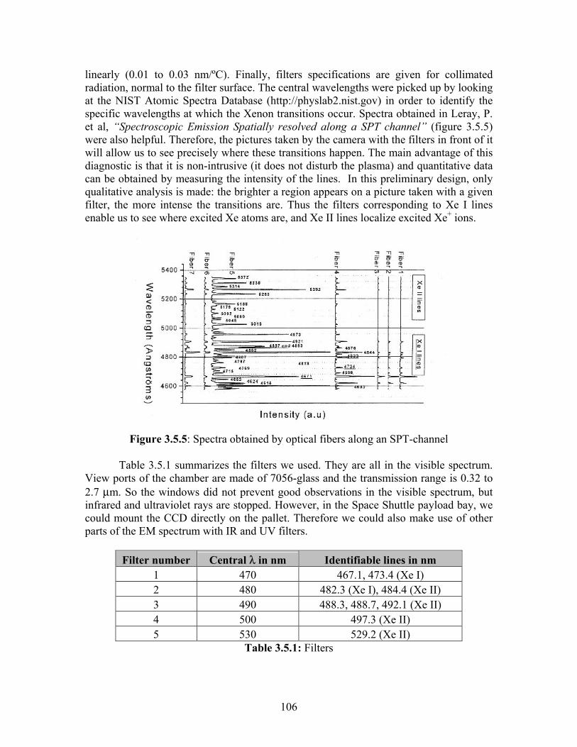
106

linearly (0.01 to 0.03 nm/ºC). Finally, filters specifications are given for collimated radiation, normal to the filter surface. The central wavelengths were picked up by looking at the NIST Atomic Spectra Database (http://physlab2.nist.gov) in order to identify the specific wavelengths at which the Xenon transitions occur. Spectra obtained in Leray, P. et al, “Spectroscopic Emission Spatially resolved along a SPT channel” (figure 3.5.5) were also helpful. Therefore, the pictures taken by the camera with the filters in front of it will allow us to see precisely where these transitions happen. The main advantage of this diagnostic is that it is non-intrusive (it does not disturb the plasma) and quantitative data can be obtained by measuring the intensity of the lines. In this preliminary design, only qualitative analysis is made: the brighter a region appears on a picture taken with a given filter, the more intense the transitions are. Thus the filters corresponding to Xe I lines enable us to see where excited Xe atoms are, and Xe II lines localize excited Xe+ ions.

Figure 3.5.5: Spectra obtained by optical fibers along an SPT-channel

Table 3.5.1 summarizes the filters we used. They are all in the visible spectrum. View ports of the chamber are made of 7056-glass and the transmission range is 0.32 to 2.7 µm. So the windows did not prevent good observations in the visible spectrum, but infrared and ultraviolet rays are stopped. However, in the Space Shuttle payload bay, we could mount the CCD directly on the pallet. Therefore we could also make use of other parts of the EM spectrum with IR and UV filters.

Filter number Central λ in nm Identifiable lines in nm

1 470 467.1, 473.4 (Xe I) 2 480 482.3 (Xe I), 484.4 (Xe II) 3 490 488.3, 488.7, 492.1 (Xe II) 4 500 497.3 (Xe II) 5 530 529.2 (Xe II)

Table 3.5.1: Filters

107

Filter 5

Filter 4

Filter 3

Filter 2

Filter 1

We took pictures of the thruster at its nominal operating point. For some of the pictures we took the negative image and/or zoomed into it in order to better identify the regions where the transitions occur (figure 3.5.6).

Figure 3.5.6: Optical emissions at the nominal operating point (0.7 mg/sec) From the first 3 pictures we can see that the spike is in front of the center cone.

Xe I transitions occur in it as well as at the exit of the channel. The annuli on the picture with filter 2 are probably due to an internal defect of the filter. From the 2 last pictures we see very intense Xe II radiations in the exit of the channel, in the spike and between these two areas. It is interesting to note that for the naked eye, the plume appears blue, so

On the negative images, wecan better see that the highconcentrations are in front ofthe exit of the channel, ANDin front of the central conewhere NO flow is exiting (i.e.in the “spike”)

108

Filter 3

Filter 2

Filter 4

Filter 5

Filter 1

the neutrals transitions (XeI) are actually contributing more to the color of the plume than ions transitions (Xe II). Finally we can use such images for more qualitative analyses. For example, the following figure (3.5.7) shows the observations we made for a Xenon flow of 0.5 mg/sec.

Figure 3.5.7: Observations for a flow of 0.5 mg/sec

109

On the left, the discharge voltage is 300 V and the magnet is on; on the right, the discharge voltage is about 100V and the magnet is off, which corresponds to an earlier step in turning on the thruster. We observe that the plume is much shorter and much wider (globally, more “spherical”) than in the nominal case. Moreover when the magnet is off, there are not any bright zones in the plume, and the filters corresponding to the Xe II wavelengths give very faint images. This is consistent with the fact that ionization in this kind of thruster is due to electrons trapped around magnetic field lines as explained in the introduction. So without the magnet there is very little ionization and thrust. Finally, once the magnet is on (images on the left), the spike is not as bright as in the nominal case.

We will not put all the images that were taken here, because the differences in

shapes are not very clear and the pictures all look pretty much the same. But table 3.5.2 summarizes the operating points we investigated. The yellow boxes indicate the parameters that were varied (thruster flow, cathode flow, discharge voltage). For each line in this table, one picture was taken with each filter (except for the last line, because the thruster stopped after the first picture only).

Test ref # Pressure C. flow mg/s

T. flow mg/s D voltage Comments

1 5.862E-06 0.1 0 0 Only cathode 2 2.034E-05 0.1 0.5 300 3 1.966E-05 0.1 0.5 300 4 2.897E-05 0.1 0.7 300 5 2.897E-05 0.1 0.7 300 Nominal 8 2.621E-05 0.1 0.6 300 12 3.31E-05 0.1 0.8 300 19 2.897E-05 0.1 0.7 300 21 2.897E-05 0.1 0.7 350 25 2.897E-05 0.1 0.7 250 31 2.862E-05 0.075 0.7 300 Only with filter 1

Table 3.5.2: Experiment with filters test matrix

To conclude, in this paragraph we proved the relevance of optical measurements.

Design-for-space issues that remain to solve are: - For the optical emissions, we need to find space-qualified CCD’s and filters. Also

we need to figure out how to mount the filters: should we use only one CCD array and change the filter in front with a filter wheel, or use a different CCD array for each filter?

- Finally, we need to find a space-qualified camera (if possible off-the-shelf).

110

111

Conclusion

All along this work, emphasis was put on instruments for the diagnostics of the interactions between electric thrusters and spacecraft. We always kept in mind the “background” which is the ETEEV Shuttle experiment and the fact that all instruments should in the end be designed according space flight specifications.

To summarize the work presented in this thesis:

• We reviewed the literature concerning instruments related to the different

objectives of the ETEEV experiment. • We gave an update on the status of the ETEEV experiment. In particular, we now

have a 3D representation of the experimental pallet, as well as detailed operational procedures; we also started the work on software engineering.

• Finally, we completed the preliminary design and testing for some of the instruments: QCM’s, Faraday Cup, Langmuir Probe and optical diagnostics.

The next step in ETEEV design is to focus more on the space qualification of the

hardware, with an emphasis on safety. We need to work in more details on payload subsystems design and software engineering: for each instrument we need to specify how it will be attached to the Hitchhiker pallet, and to make sure the whole assembly withstands the launch loads and the harsh space environment. Finally, we will be able to have precise specifications of data rates and power needed for each instrument. In the end, an engineering model of the ETEEV payload should be ready about a year and a half from now (late 2003).

When that major milestone is accomplished, the remaining ground experiments will consist in recording canonical data (in the best ground facilities available) prior to the flight: this data is to be compared to flight data. We would also retake a set of data after the flight, to see if the system was modified by the flight.

The following tables summarize the subsequent work to be done on each instrument (names in italic indicate already space-qualified hardware).

112

Instrument To do

QCM Finish collimator construction Mounting and testing in the chamber (cooling system?) In-space mounting, shuttering, data acq. and temperature control Detailed specifications (data rate, power) Witness plates Calculations for predicted erosion rates (from FC and energy data) Selection of materials to test Test in chamber with collimator In-space mounting and shuttering FC and QLP Strengthen the current designs to meet space qualification specs Attachment to MDB and in-space data acquisition Detailed specifications (data rate, power) Emissive probe Build and test a prototype in lab Design for space-qualification, attachment to MDB, data acq. Detailed specifications (data rate, power) Thrust balance Build and test a prototype in lab Detailed specifications (data rate, power) Video camera & Select hardware from commercially available offers CCD with filters (if possible already space qualified) CCTV cameras Confirm availability from NASA DIDM Confirm availability from AFRL Pressure sensor Select from commercially available (space qualified)

Other items To do

Mechanical Build and test a prototype in lab Diagnostics In-space mounting and control Boom Space qualification of the concept Operational GRAFCETs for all parts of the experiment procedures Detailed experimental protocoles Selection of the operating points to be tested Software Finish level 1 and 2 of the Intent Specification engineering Build blackbox behavior model Run simulations to check for software safety Write code

113

Bibliography In order of appearance: 1.1) [1] McKeown, D., “Quartz crystal instrumentation for space research”, SPIE Conference on Optical Systems Contamination: Effects, Measurements, and Control VI, SPIE Vol. 3427, 1998. [2] Uy, M. O. et al., “Miniature Quartz Crystal Microbalance for Spacecraft and Missile Applications”, John Hopkins APL Technical Digest, Vol. 20, No. 2, 1999. [3] Wallace, D. A., and Wallace, S. A., “First tests of an extremely high-mass sensitivity, miniature TQCM which is impervious to solar thermal radiation effects”, SPIE Conference on Optical Systems Contamination: Effects, Measurements, and Control VI, SPIE Vol. 3427, 1998. [4] Fountain, J. A., “Temperature-controlled quartz crystal microbalance measurements on Space Transportation System (STS-2)”, SPIE Vol. 338. [5] Absalamov, S. K. et al., “Measurement of plasma parameters in the Stationary Plasma Thruster (SPT-100) plume and its effect on spacecraft components”, AIAA 92-3156, 28th AIAA/ASME/SAE/ASEE Joint Propulsion Conference. [6] Randolph, T., Pencil, E. J., and Manzella, D. H., “Far-field plume contamination and sputtering of the stationary plasma thruster”, AIAA 94-2855, 30th AIAA/ASME/SAE/ASEE Joint Propulsion Conference. [7] Pencil, E. J., Randolph, T., and Manzella, D. H., “End-of-Life Stationary Plasma Thrusters Far-field Plume Characterization”, AIAA 96-2709, 32th AIAA/ASME/SAE/ASEE Joint Propulsion Conference.

114

[8] Jaworske, D. A., “Hall Effect Thruster Plume Contamination and Erosion Study”, NASA/TM-2000-210204, June 2000. [9] Winquist, G. A., Partridge, J. M., “Faraday Probe Design for the Vacuum Arc Ion Thruster”, Major Qualifying Project Report, Worcester Polytechnic Institute, July 2001. [10] Sosolik, C. E., et al., “A technique for accurate measurements of ion beam current density using a Faraday Cup”, Review of Scientific Instruments, Vol. 71 No 9, September 2000. [11] Hofer, R. R., et al., “A comparison of Nude and Collimated Faraday Probes for Use with Hall Thrusters”, 2001 International Electric Propulsion Conference, IEPC 01-20. [12] King, L. B., Gallimore, A. D., “Gridded retarding pressure sensor for ion and neutral particle analysis in flowing plasmas”, Review of Scientific Instruments, Vol. 68 No 2, February 1997. [13] Marrese, C. M., et al., “Development of a Single-orifice Retarding Potential Analyser for Hall Thruster Plume Characterization”, IEPC 97-066. [14] Fife, J. M., “Hybrid-PIC Modeling and Electrostatic Probe Survey of Hall Thrusters”, PhD Thesis, Massachusetts Institute of Technology, September 1998. [15] Haas, J. H., et al., “An Investigation of Electrostatic Probe Perturbations on the Operational Characteristics of a Hall Thruster and on the Measurement of Local Plasma Parameters”, AIAA 98-3656. [16] Eckman, R., et al., “Triple Langmuir Probe Measurements in the Plume of a Pulsed Plasma Thruster”, Journal of Propulsion and Power, Vol. 17, No. 4, July-August 2001. [17] Tilley, D. L., “The adverse effect of perpendicular ion drift flow on cylindrical triple probe electron temperature measurements”, Rev. Sci. Instrum. 65 (3), March 1994. 1.2) [18] Manzella, D., et al., “Performance Evaluation of the SPT-140”, IEPC 97-0589. [19] Hargus, W., et al., “Preliminary Preformance Results of the High Performance Hall System SPT-140”, AIAA 2000-3250, 36th AIAA/ASME/SAE/ASEE Joint Propulsion Conference.

115

1.3) [20] Sovey, J. S., et al., “Electromagnetic Emission Experiences Using Electric Propulsion Systems”, AIAA 87-2028, 23rd AIAA/ASME/SAE/ASEE Joint Propulsion Conference. [21] Sarmiento, C. J., et al., “RHETT2/EPDM Hall Thruster Propulsion System Electromagnetic Compatibility Evaluation”, IEPC 97-108. [22] Gilchrist, B. E., et al., “Electromagnetic Wave Scattering Experiments in Hall Thruster Plasma Plumes”, AIAA 98-3642, 34th AIAA/ASME/SAE/ASEE Joint Propulsion Conference. [23] Davis, C. N., et al., “Density and Spectral Measurements using a 34 GHz Interferometry System”, AIAA 99-2718. [24] Onodera, N., et al., “Interaction between Plasma Plume of Electric Propulsion and Spacecraft Communication”, IEPC 99-228. [25] Hallock, G. A., et al., “Impact analysis of Hall Thrusters on Satellite Communication”, AIAA 2000-3519, 36th AIAA/ASME/SAE/ASEE Joint Propulsion Conference. [26] Loane, J. T., et al., “Analysis of Communication Signal Modulation Induced by Periodic Hall Thruster Plume Instabilities”, IEPC 01-58. [27] Plokhikh, A. P., et al., “Methods for Investigating the Influence of Self-Induced Electromagnetic Emission of Electric Propulsion Upon the Sensitivity Characteristics of Onboard Radio Systems of Spacecrafts”, IEPC 01-257. [28] Beiting, E. J., et al., “Electromagnetic Emissions from a BHT-200 Hall Thruster”, IEPC 01-342. [29] Leray, P., et al., “Spectroscopic Emission Spatially Resolved along a SPT Channel”, Proceedings of 2nd Europ. Spacecraft Propulsion Conf., 1997, pp. 447-453. [30] Karabadzhak, G., et al., “Optical Emission of a Hall Thruster Plume in Space Condition”, IEPC 01-053. 1.4) [31] Bromaghim, D. R., et al., “An Overview of the On-orbit Results from the Electric Propulsion Space Experiment (ESEX)”, IEPC 99-182. [32] Manzella, D., et al., “Hall Thruster Plume Measurements On-board the Russian Express Satellites”, IEPC 01-044

116

[33] Boyd, I. D., “Hall Thruster Far Field Plume Modeling and Comparison to Express Flight Data”, AIAA 2002-0487,40th AIAA Aerospace Sciences Meeting and Exhibit. [34] Capacci, M., et al., “An Electric Propulsion Diagnostic Package for the Characterization of the Plasma Thruster/Spacecraft Interactions on STENTOR Satellite”, AIAA 99-2277, 35th AIAA/ASME/SAE/ASEE Joint Propulsion Conference. [35] Darnon, F., et al., “Plasma Propulsion on STENTOR Satellite: In-flight Acceptance Operations and Experimental Program”, IEPC 01-167. 2.2) [36] Azziz, Y., Master of Science Thesis in progress, Massachusetts Institute of Technology. 2.3) [37] Mirczak, J., “A Milli-Newton Thrust Stand for Space Shuttle Flights”, Master of Science Thesis in progress, Massachusetts Institute of Technology. [38] Thomas, S., “Developing a Space Shuttle Experiment for Hall and Pulsed Plasma Thrusters”, Master of Science Thesis, Massachusetts Institute of Technology, February 2001. 2.4) [39] Suryali, A., et al., “Ground and Space PPT Plume Experiments”, Major Qualifying Project Report, Worcester Polytechnic Institute. 2.6) [40] Leveson, N., “Intent Specifications: An Approach to Building Human-Centered Specifications”, http://sunnyday.mit.edu/papers.html [41] Leveson, N., Reese, J. D., “Sample TCAS Intent Specification”, http://sunnyday.mit.edu/papers.html 3.3) [42] Cheng, Shannon Y. M., “Computational Modeling of a Hall Thruster Plasma plume in a vacuum tank”, Master of Science Thesis, Massachusetts Institute of Technology, February 2002. 3.4) [43] Zwahlen, J., “Quadruple Langmuir Probe Measurements in the Plume of a Teflon Pulsed Plasma Thruster”, Master of Science Thesis in progress, WPI.

117

Appendixes

Appendix A. Acronyms AFRL Air Force Research Laboratory BOL Beginning Of Life CARS Customer Accomodations and Requirements Specifications CCD Charge Coupled Device CCTV Closed Circuit Television CEX Charge Exchange CPR Customer Payload Requirements DBP Double Bay Pallet DIDM Digital Ion Drift Meter EMI Electromagnetic Interferences EOL End Of Life EP Emissive Probe ETEEV Electric Thrusters Environmental Effects Verification FC Faraday Cup GRAFCET Graphe de Commande Etape-Transition (French for "Graph of Command by Steps and Transitions") HH Hitchhiker LP Langmuir Probe MDB Mechanical Diagnostics Boom PPT Pulsed Plasma Thruster QCM Quartz Crystal Microbalance

118

QLP Quadruple Langmuir Probe RPA Retarding Potential Analyser SLP Single Langmuir Probe SpecTRM-RL Specification Tool and Requirements Methodology - Requirements Language SPT Stationary Plasma Thruster SSPP Shuttle Small Payloads Projects WP Witness Plate

119

Appendix B. NASA Documents

Hitchhiker References Shuttle Small Payloads Project Office (at Goddard Space Flight Center): http://sspp.gsfc.nasa.gov/ Particularly in the “Documents” section: Carrier Capabilities Document: http://sspp.gsfc.nasa.gov/documents/sspp_brochure20p.pdf CARS (Customer Accommodations & Requirements Specifications) Document: http://sspp.gsfc.nasa.gov/documents/CARS.pdf

Shuttle References More general documents for the Space Shuttle Payloads can be found on the following site: http://shuttlepayloads.jsc.nasa.gov/data/Overview/Overview.htm More specifically, under the “Payload Documentation” section: The Space Shuttle NSTS 21492, Payload Bay Payload User's Guide, is intended to familiarize Payload Customers with the capabilities and services offered, as well as the integration process. http://shuttlepayloads.jsc.nasa.gov/data/PayloadDocs/documents/21492.pdf Volume XIV of the NSTS 07700 Program Definitions & Requirements describes Space Shuttle Payload Accommodations. It is composed of several chapters, and appendixes are also important: Appendix 1, Contamination Environment Appendix 2, Thermal Appendix 3, Electrical Power and Avionics Appendix 4, Structures and Mechanics Appendix 5, Ground Operations Appendix 6, Mission Planning and Flight Design Appendix 7, Extravehicular Activities Appendix 8, Payload Deployment and Retrieval Appendix 9, Intravehicular Activities Appendix 10, Integration Hardware http://shuttlepayloads.jsc.nasa.gov/data/PayloadDocs/documents/07700/Vol_XIV.pdf

120

Links to safety documents are included in the “Payload Documentation” and in the “Safety Data” sections. Also NSTS 22254 (Methodology For Conduct of Space Shuttle Hazard Analysis) must be consulted. The “Technical Analysis” section contains information about: Structural Analysis: NSTS 37329, Structural Integration Analyses Responsibility Definition for Space Shuttle Vehicle and Cargo Element Developers: http://shuttlepayloads.jsc.nasa.gov/data/payloaddocs/documents/37329.pdf NSTS 14046, Payload Verification Requirements: http://shuttlepayloads.jsc.nasa.gov/data/payloaddocs/documents/14046.pdf Thermal Analysis: JSC 14686, Criteria/Guidelines For Payload Thermal Math Models For Integration Analysis. Electromagnetic Compatibility Analysis: NSTS 21288, Required Data/Guidelines For Payload/Shuttle Electromagnetic Compatibility Analysis http://shuttlepayloads.jsc.nasa.gov/data/payloaddocs/documents/21288.pdf Also SL-E-0001 (Specification Electromagnetic Compatibility Requirement) is useful: http://procure.msfc.nasa.gov/jsc/IVEST/SL-E-0001D.pdf The “Digital Models” section explains that a 3-Dimensional (3-D) Computer Aided Design (CAD) model of every payload is required and gives guidelines on how to make such drawings. Finally, information on the CCTV (Closed Circuit Television System) cameras can be found at: http://spaceflight.nasa.gov/shuttle/reference/shutref/orbiter/comm/inst/cctv.html

121

Appendix C. Documentation for laboratory hardware

C1. Vacuum chamber instructions Special items

- Wear cotton gloves while working in the chamber (DO NOT touch the inside with bare hands)

- Cover the pumps with small grids (DO NOT forget to remove the covers when pumping down).

- If necessary, clean the chamber surfaces with alcohol using paper towels. DO NOT put alcohol on the O-Rings.

- If the mechanical pump smokes, check the filter (a little bit of bad smell is OK). Starting the Cryopumps and Pumping (General Case)

Initial state: Atmospheric Pressure,

Cryopumps warm. Check air supply: open.

While cooling down: Close OB400 Regen valve.

Open rough valve. Reduce pressure to 10-100 mTorr on TC2. Wait from “Completion” message (>2 hrs).

Check N2 gauge: open, 40 psi Check water supply: open.

Turn on Cryos, close CT10 Regen valve. Perform OB400 regeneration: press REGEN

button and 02. Wait for “cooling down” message.

All valves closed, Main door closed and

Lightly clamped.

Turn on mechanical pump. Wait until TC1 ≈ 1.1x10-2

Open cryo Regen valves. Pump to 10 – 20 mTorr on

TC1.

Close Rough valve. Shut off mechanical pump.

Open Cryo valves. Monitor cold cathode on TC1, (EMIS)

122

Turning on the Cryopumps without Regeneration

Pumping When the Cryos are Already Cold

Check there is water and turn the CT10 and OB400 water valves on.

Open both Regen Valves, wait ½ hour, close valves.

Turn on the mechanical pump, wait until TC1 ≈ 1.1x10-2

Open CT10 Regen valve, wait until TC1 is back at ≈ 10-2, close the valve.

Turn on the pumps with switches (and panel for OB400: control + 1)

Open OB400 Regen valve; wait until TC1 is back at ≈ 10-2, close the valve.

Then if need to pump down, follow “pumping” instructions.

Close the chamber door. Wait until TC1 is down again.

Turn the mechanical pump on. Close the Rough valve.

Wait until TC1 ≈ 1.1x10-2 Open the Cryo valves.

Monitor pressure with TC1 (down to 10-3 torr, then wait some more and turn on EMIS when pressure ~ 10-5 (Not at

too high pressure)

Open the Rough valve.

123

Venting the Chamber Shutting Down the Cryos

In Case of Condensation on the Pumps (Feels Slippery/Icy when you touch them):

Flip “Vent Chamber” switch. Chamber is done when rushing sound stops.

1. Chamber is under vacuum 2. Rough valve is closed 3. Cryo valves are closed 4. Door is lightly clamped 5. Chamber heat is off

Shut down CT10 with the switch. Open the Regen valves

Shut down OB400 with the switch, then with the panel

(control + 0).

Wait ≈ 1 hour

Close the valves.

Turn on the mechanical pump. Turn the mechanical pump off.

Turn mechanical pump on. Watch TC1 going up then down again.

Close Regen valve(s). Watch TC1 going down to ≈ 1.1x10-2

Shut off mechanical pumps. Open Regen valve(s).

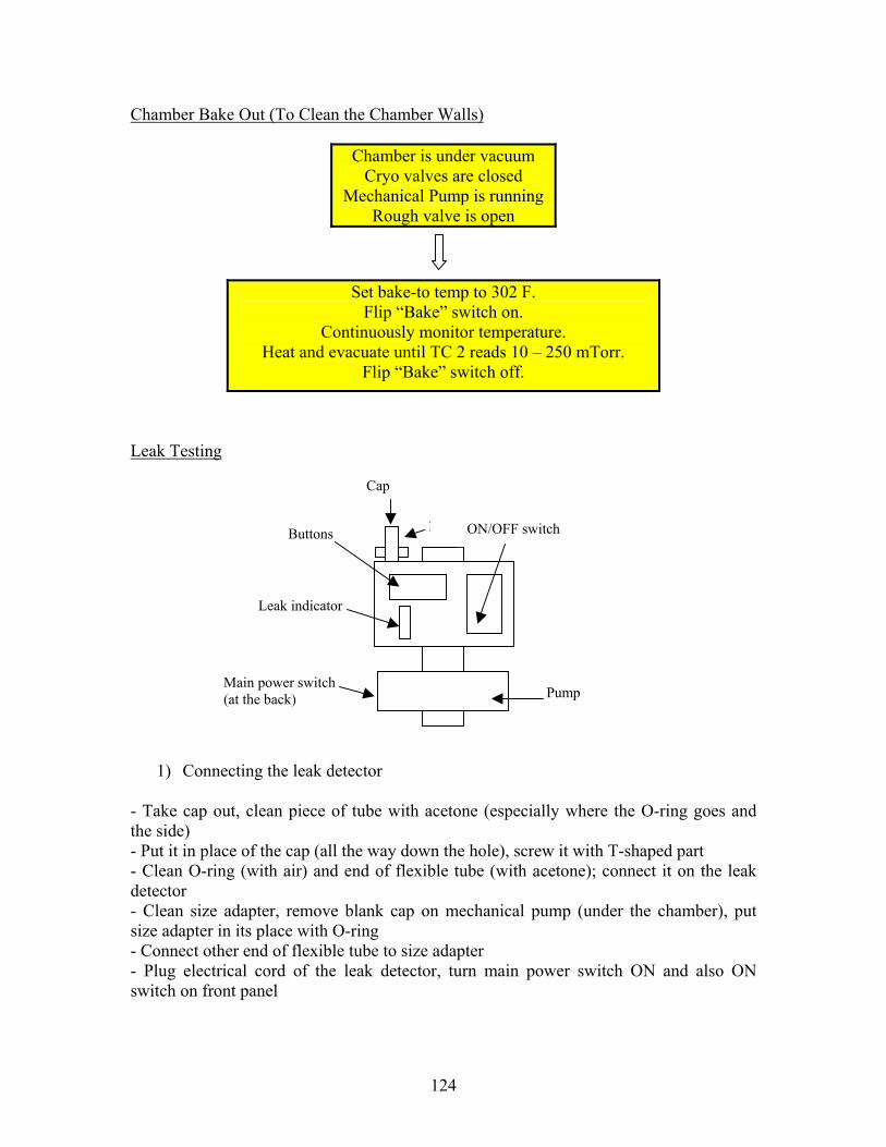
124

Chamber Bake Out (To Clean the Chamber Walls) Leak Testing

1) Connecting the leak detector - Take cap out, clean piece of tube with acetone (especially where the O-ring goes and the side) - Put it in place of the cap (all the way down the hole), screw it with T-shaped part - Clean O-ring (with air) and end of flexible tube (with acetone); connect it on the leak detector - Clean size adapter, remove blank cap on mechanical pump (under the chamber), put size adapter in its place with O-ring - Connect other end of flexible tube to size adapter - Plug electrical cord of the leak detector, turn main power switch ON and also ON switch on front panel

Chamber is under vacuum Cryo valves are closed

Mechanical Pump is running Rough valve is open

Set bake-to temp to 302 F. Flip “Bake” switch on.

Continuously monitor temperature. Heat and evacuate until TC 2 reads 10 – 250 mTorr.

Flip “Bake” switch off.

Buttons ON/OFF switch

Leak indicator

Pump Main power switch (at the back)

Cap

1

125

2) Testing - Start mechanical pump - Check all valves closed - Open rough valve - Wait until TC2 drops to 10 to 15 mtorr - Press Start button on leak detector - Spray helium near “1” to make sure there is no big leak there - If OK, spray helium in places to be tested - When done, press hold

3) Disconnecting the leak detector - Rough valve OFF - Mechanical pump OFF - Double check all the valves are closed - Press vent button on leak detector - Switch leak detector off, unplug it and put all the “plumbing stuff” back in place (don’t forget to put back the cap on the mechanical pump below the chamber!) CT-10 Manual Regeneration

1) Connect the “Assembly for CT-10 regeneration” to the nitrogen tank. 2) At the bottom of the CT-10:

(a) Disconnect the flexible tube going to the mechanical pump (b) Unscrew the other end of the “ T”

3) Take the cap from the leak testing port on the mechanical pump, and use the size

adapter found in the leak detector accessories to put the cap in place of the flexible pipe disconnected in (2a).

4) Put the “Regen connector” inside the part unscrewed in (2b).

5) Connect the “Assembly for CT-10 regeneration” and the “Regen connector” by a

Teflon tube.

6) Let nitrogen flow in the CT-10 for about 20 minutes (at 20 psi). When putting everything back in place do not forget to put back the cap on the leak testing port!

126

Chamber diagram

C2. Thruster instructions GRAFCETs of cathode and thruster operation are on the following pages.

Control Box

Mechanical Pump

Leak Test PortRoughing (Rough) Valve

Chamber Vent

CT10 Regen Valve OB400 Regen Valve

TC1 (Thermocouple)

Chamber Door

CT10 Cryo Valve

Thermocouple TC2

Cold Cathode TC1/CC

OB400 CT10

OB400 Cryo Valve

Water

Water

Water

127

CATHODE FIRST RUN

Heater current = 6.5 A, voltage ~ 6.5 V

Keeper current = 0A

Open cathode vacuum valve

Turn on heater power supply

Increase keeper voltage to 75 V

Turn off heater

Startup configuration: all valves shut,cathode cold, thruster off, powersupplies off. Chamber under vacuum.Water on target on.

Start command received

Keeper current around 0.7A, voltage around 20V

Cathode standby mode Go to thruster operation diagram

Open Xe tank

Open cathode upstream valve

Open cathode flowmeter @ 1 sccm

0

1

2

3

4

5

6 In current controlled mode,increase current by 0.5 A every halfhour, starting at 2 A

7 Keep heater current at 6.5A andturn on keeper power supply (setit to 0 V)

8

9

Cathode flowmeter ON @ 1 sccm . t/4/60 min (Wait for lines to fill up 60 minutes)

Cathode vacuum valve open (manual tell when OK; in flight electrovalve)

Xe tank open (manual tell when OK; in flight electrovalve)

Cathode upstream valve open (manual tell when OK; in flight electrovalve)

10

Heater current = 0

Heater power supply ON

Keeper power supply ON @ 0V

9’ Increase cath. flow to 2 sccm (if already, go to troubleshooting)

128

129

CATHODE SUBSEQUENT RUN

Heater current = 6 A

Keeper current = 0A

Open cathode vacuum valve

Turn on heater power supply

Increase keeper voltage to 75 V

Turn off heater

Startup configuration: all valvesshut, cathode cold, thruster off,power supplies off. Chamber undervacuum. Water on target on.

Start command received

Keeper current = 0.7A

Cathode standby mode Go to thruster operation diagram

Open Xe tank

Open cathode upstream valve

Open cathode flowmeter @ 1 sccm

0

1

2

3

4

5

6 In current controlled mode, put it at2A for 1 hour, then 4A for 30 min,then 6A.

7 Keep heater current at 6A andturn on keeper power supply (setit to 0 V)

8

9

Cathode flowmeter ON @ 1 sccm . t/4/10 min (Wait for lines to fill up 10 minutes)

Cathode vacuum valve open (manual tell when OK; in flight electrovalve)

Xe tank open (manual tell when OK; in flight electrovalve)

Cathode upstream valve open (manual tell when OK; in flight electrovalve)

10

Heater current = 0

Heater power supply ON

Keeper power supply ON @ 0V

Increase cath. flow to 2 sccm (if already, go to troubleshooting)

9’

130

131

THRUSTER START

Discharge voltage 100 V

Open thruster vacuum valve

Turn on discharge power supply (current limited mode)

Turn on magnet p.s. and increasemagnet current

Startup configuration: all valves shut,cathode in standby mode, thrusteroff, discharge and magnet powersupplies off. Chamber under vacuum.Water on target on. Start command received

Discharge current is down to ~ 500mA

Open thruster upstream valve

Open thruster flowmeter @ 5 sccm

0

1

2

3

4

5 Current limit the discharge p.s. to 1.5A and increase voltage to 100V

6 Increase discharge voltage until itswitches to current limited mode

7

Thruster flowmeter ON @ 5 sccm . t/3/5 min (Wait for lines to fill up 5 minutes)

Thruster upstream valve open (manual tell when OK; in flight electrovalve)

Increase discharge voltage to 300V 8

Discharge power supply ON

Discharge starts (purple glow)

Thruster vacuum valve open (manual tell when OK; in flight electrovalve)

Discharge current = 1.5A

Increase magnet current to 0.4 Aand discharge voltage to 300 V (atthe same time)

9

132

133

THRUSTER RESTART (after 1 to 1.5 h of operation, the power decreases due to surface conditioning: then we restart the thruster at its nominal operating point)

Thruster ON 11

Keeper current = 200 mA

10

Magnet current = 0.4 A and discharge voltage = 300 V (blue glow)

Reduce cathode keeper currentto 200 mA

Open thruster vacuum valve

Turn on discharge power supply (current limited mode)

Startup configuration: all valves shut,cathode in standby mode, thruster off (hasrun for 1 hour already at 5 sccm), dischargeand magnet power supplies off. Chamberunder vacuum. Water on target on. Start command received

Open thruster upstream valve

Open thruster flowmeter @ 7.12 sccm

0

1

2

3

4

5 Current limit the discharge p.s. to 1.5A and increase voltage to 100V

Thruster flowmeter ON @ 5 sccm . t/3/5 min (Wait for lines to fill up 5 minutes)

Thruster upstream valve open (manual tell when OK; in flight electrovalve)

Discharge power supply ON

Thruster vacuum valve open (manual tell when OK; in flight electrovalve)

134

135

Discharge voltage 100 V

Turn on magnet p.s. and increasemagnet current slowly

Discharge current is down to ~ 500mA

6 Increase discharge voltage to300V

7

Increase discharge voltage 8

Nominal thruster operation11

Keeper current = 0 A

Discharge starts (purple glow)

Discharge current = 1.5AIncrease magnet current to 0.4 Aand discharge voltage to 300 V (atthe same time)

Magnet current = 0.4 A and discharge voltage = 300 V (blue glow)

Turn off cathode keeper current

9

10

136

137

THRUSTER SHUTDOWN To turn off the cathode as well:

Reduce cathode heater current to 0 A Reduce cathode keeper current to 0 A Close cathode vacuum valve Set cathode flowmeter to zero Close cathode upstream valve Close Xe tank.

On the ground, turn off water on target.

Thruster flow = 0 sccm

Set keeper current to 0.7A (itsstandby mode)

Close thruster vacuum valve

Thruster OFF

Thruster ON

Shut down command received

Reduce discharge voltage to 0 V

Reduce magnet current to 0 A

0

1

2

3

4

6 Set thruster flowmeter to 0 sccm

7 Close thruster upstream valve

8

Magnet current = 0 A

Discharge voltage = 0 V

Thruster vacuum valve closed

Upstream valve closed

Keeper current = 0.7 A

138

139

C3. Arm and step motor instructions

The step motor is operated by a controller connected to a computer via a serial link. The program is in BASIC and its name is MODIFBIS.BAS. It is possible to run it with the QuickBasic software. The controller has an EEPROM memory on which a test sequence for the motor is written. This test sequence is performed every time the controller is turned on. It can be modified by modifying MODIFBIS.BAS and then uploading the changes in the EEPROM memory, but the current version is optimized for operation in the chamber (so that the arm does not hit the bridge, etc…) First run 0 – arm NOT on the motor, crosspiece positioned at desired radius with appropriate counterweight, sensor wires disconnected, controller off, program not running. Chamber open. 1 – position the shaft so that the flat part is on the right (when looking in the chamber). 2 – put the arm on the shaft and tighten the set-screw (the set screw should touch the shaft on the flat part. Check that the arm is leveled. 3 – put something in the home sensor to block it, turn the controller on: the arm starts rotating clockwise. Remove the block as soon as possible (before the arm hits the bridge). 4 – wait till end of EEPROM programmed sequence (when LEDs B2, B0 and DR are lit). 5 – start MODIFBIS.BAS program (in Program Files/Quickbasic/Stepmotor directory) with Quickbasic: open program, then run (F5). 6 – make a few steps with the motor to adjust arm into position zero (all the way to the left when looking in chamber). Set this as P=00000000 for the program (command A 0). 7 – connect sensor wires and check it works (check continuity). Also make sure the wires do not prevent proper arm motion. 8 – arm is now ready to be piloted to desired position and acquire data. 9 – close the tank, pump down chamber.

140

Subsequent runs (this procedure is applicable if the controller has not been switched off, even if the program has been stopped) 0 – arm on the motor, crosspiece positioned at desired radius with appropriate counterweight, sensor wires connected, controller on, program not running. Chamber under vacuum. 1 – run program MODIFBIS.BAS (in Program Files/Quickbasic/Stepmotor directory) with Quickbasic. Use Shift+F5 instead of F5 (for the program it is actually a restart, not a start). 2 – verify that display is P=00000000 when the arm is at position 0 (need to check that as precisely as possible through the window) 3 – arm is now ready to be piloted to desired position and acquire data Subsequent runs (if controller has been shut down) 0 – arm on the motor, crosspiece positioned at desired radius with appropriate counterweight, sensor wires connected, controller off, program not running. Chamber under vacuum. 1 – put something in the home sensor to block it, turn the controller on: the arm starts rotating clockwise. Remove the block as soon as possible (before the arm hits the bridge). 2 – wait till end of EEPROM programmed sequence (when LEDs B2, B0 and DR are lit). 3 – start MODIFBIS.BAS program (in Program Files/Quickbasic/Stepmotor directory) with Quickbasic: open program, then run (F5). 4 – if needed make a few steps with the motor to adjust arm into position zero (all the way to the left when looking in chamber). Set this as P=00000000 for the program with command A 0 (need to check that as precisely as possible through the window). 5 – arm is now ready to be piloted to desired position and acquire data. IMPORTANT When turning the controller off make sure the arm is positioned between positions 0 and 90 degrees. Otherwise, the EEPROM program may send the arm banging into the right side of the bridge.

141

MOTOR COMMANDS MOTION PARAMETERS F 1 Sets the First (starting) speed of motor to 1 (default = 15) ? F Returns the current value of F S 1 Sets the Slope (acceleration) of motor to 1 (default = 225) ? S Returns the current value of S R 2 Sets the Ramp (maximum) speed of motor (default = 125) ? R Returns the current value of R The range is 0 to 255 max. (20 to 20000 pulses per second) INCREMENTAL MOVE COMMANDS N 20 Sets the number of steps taken for each GO command (here, 20) ? N Returns the current value of N + Sets the direction of a GO move to clockwise - Sets the direction of a GO move to counterclockwise G GO command (go N steps in the specified direction) After a GO command, the motor knows its position (? P or F9) ABSOLUTE MOVE COMMANDS P 20 Moves to absolute position 20 ? P Returns the current position (or F9) A 10 Sets the position counter to 10 H 1 Causes the motor to home to origin using input B1 (speed=1/20 of F) With absolute move, it is not possible to choose the direction of rotation. Positions are “labeled” clockwise so if P increases, moves clockwise, and if P decreases, moves counterclockwise.

Clockwise = + Counterclockwise = -

142

CORRESPONDANCE BETWEEN ANGLE AND STEPS

Angle of rotation Number of steps

5 22.2

10 44.4

15 66.7

20 88.9

25 111.1

30 133.3

35 155.6

40 177.8

45 200.0

50 222.2

55 244.4

60 266.7

65 288.9

70 311.1

75 333.3

80 355.6

85 377.8

90 400.0

143

C4. Single Langmuir Probe (SLP) The Single Langmuir Probe that we bought from Hiden Analytical was installed in one of the feedthroughs of the vacuum chamber. It is then connected to its controller via a coaxial cable. This controller has only one front panel switch (on/off). The controller is connected to the desktop computer by a serial link (RS-232), and the software ESPsoft is installed there and commands the voltage sweeps as well as the data acquisition. Then how to run an experiment is explained in the manuals of the probe and of the software. The important steps are: 1) Create the acquisition parameters file (.PRM):

For example the acquisition parameters used for the experiment described in paragraph 3.4 were: File name: Matrix “test number” “scan number” Ion weight: 131.29 g/mol Probe area: 4.7 mm2 Number of scans per run: 1 Gain range: 0.1 mA Autoranging disabled (not checked) Method of acquiring data: User defined parameters Zstage: No Then for user defined parameters setup: Potential ramp: Start: –50 V, Stop: +50 V Samples per scan: 201 (i.e. every 0.5 V) Timing: Sample Dwell Time: 10 ms (time it stays at a given voltage) Start Dwell: 10 ms (time it waits before recording current) Min cycle period: 1000 ms Cleaning: Pre scan clean period: 0.0 ms Cleaning potential: 0.00 V Gain range: 0.1 mA Expt Park Potential: 0 V (tip voltage between scans) Idle Park Potential: Use Vf (i.e open circuit when parked) 2) Create the experiment file (.ESP) also called “Design of Experiment” in the manual:

There the user creates the test matrix for his experiment. He has to define the parameters (in our case, flow rate, discharge voltage, etc) and these parameters will be put in the columns of the matrix. Then, each different set of parameters is called a “run” and is listed in the lines of the matrix. As many runs as needed can be inserted with the command “insert run”.

144

3) “Acquire Run”: taking the data. 0 – Turn the SLP on (switch on controller front panel), then launch ESPsoft; open the experiment file (“matrix.esp” for the experiment we did) and verify the “acquisition parameters” (in Probe/Edit). 1 – Put the thruster in the desired operating point (from the parameter values given in the test matrix) and wait 5 minutes for stabilization of the conditions. 2 – Do “setup run parameters”, then “acquire run” and save. The data is the I-V curve stored in a .LDA file. 3 – Change the operating point of the thruster, then redo the same operation, fo rall the other lines in the test matrix. 4) “Analyze Run”: automatic analysis of the data.

The user can define his “Fit Parameters” (those that will be used to find plasma parameters from the .LDA file). Then, different results can be displayed:

- I-V curve - Scan report (containing the calculated values of Vf, Vp, Te, ne, ni, Debye length

and electron energy distribution parameters) - Trend report - EED profile

Each of these can be printed and saved. Finally, all the data (from the run and from the subsequent analysis) can be save in .DAT format, which enables exportation to usual data exploitation software like Microsoft Excel.