A New Flare Combustion and Plume Rise Model - University ...
148
University of Calgary PRISM: University of Calgary's Digital Repository Graduate Studies The Vault: Electronic Theses and Dissertations 2012-12-14 Plume Dispersion: A New Flare Combustion and Plume Rise Model Rahnama, Kamran Rahnama, K. (2012). Plume Dispersion: A New Flare Combustion and Plume Rise Model (Unpublished master's thesis). University of Calgary, Calgary, AB. doi:10.11575/PRISM/27371 http://hdl.handle.net/11023/357 master thesis University of Calgary graduate students retain copyright ownership and moral rights for their thesis. You may use this material in any way that is permitted by the Copyright Act or through licensing that has been assigned to the document. For uses that are not allowable under copyright legislation or licensing, you are required to seek permission. Downloaded from PRISM: https://prism.ucalgary.ca
-
Upload
khangminh22 -
Category
Documents
-
view
1 -
download
0
Transcript of A New Flare Combustion and Plume Rise Model - University ...

University of Calgary
PRISM: University of Calgary's Digital Repository
Graduate Studies The Vault: Electronic Theses and Dissertations
2012-12-14
Plume Dispersion: A New Flare Combustion and
Plume Rise Model
Rahnama, Kamran
Rahnama, K. (2012). Plume Dispersion: A New Flare Combustion and Plume Rise Model
(Unpublished master's thesis). University of Calgary, Calgary, AB. doi:10.11575/PRISM/27371
http://hdl.handle.net/11023/357
master thesis
University of Calgary graduate students retain copyright ownership and moral rights for their
thesis. You may use this material in any way that is permitted by the Copyright Act or through
licensing that has been assigned to the document. For uses that are not allowable under
copyright legislation or licensing, you are required to seek permission.
Downloaded from PRISM: https://prism.ucalgary.ca

UNIVERSITY OF CALGARY
Plume Dispersion: A New Flare Combustion and Plume Rise Model
by
Kamran Rahnama
A THESIS
SUBMITTED TO THE FACULTY OF GRADUATE STUDIES
IN PARTIAL FULFILMENT OF THE REQUIREMENTS FOR THE
DEGREE OF MASTER OF SCIENCE
CHEMICAL AND PETROLEUM ENGINEERING DEPARTMENT
CALGARY, ALBERTA
December, 2012
© Kamran Rahnama 2012

ii
Abstract
Air pollution from industrial sources is a continuing concern, especially near residential areas,
where public health can be affected. Dispersion of plumes released from stacks depends on wind
speed, plume emission rate, stack height, and other meteorological and stack variables. Plume
rise is an important aspect of plume dispersion because it increases the apparent release height,
which leads to lower ground-level concentrations. Plume rise models are therefore important
components of air dispersion models. Plume rise linked with flare combustion has received only
minimal attention in the scientific literature to date, despite its importance.
This thesis develops a numerical model of plume rise with flare combustion based on material,
heat, mass, and momentum balances. The basis of the model was proposed by Scire et al. (2000)
as Plume Rise Model Enhancements (PRIME) for plume rise and building downwash. Later on,
De Visscher (2009) extended the PRIME model to account for flare combustion by keeping track
of the amount of oxygen mixed into the plume. The current study is an extension of the work of
De Visscher (2009) to account for the rate of reaction. The proposed model considers the
reaction kinetics to produce more realistic and accurate results. Moreover, emissivity, which
plays an important role in the heat conservation equations but which was only parameterized in
the original model, is calculated explicitly to increase the accuracy of the model.
In the first step, a set of heat, material, and momentum conservation equations are proposed
related to the wind speed and the stack parameters. The basic model is obtained by solving these
equations simultaneously assuming instantaneous combustion. Then the kinetics of combustion
to CO and CO2 were considered as a model extension. The emissivity calculation was also
enhanced to obtain more accurate results in the improved model. Finally, the air dispersion
model CALPUFF was run according to the proposed flare model and a simpler and less realistic
flare model by Beychok (2005) to compare results of the models.
This new flare method is simple enough to be embedded into the air dispersion modeling
software (such as CALPUFF). Currently, regulatory models use variants of Beychok’s (2005)
approach, but these are not realistic. More sophisticated models exist (e.g. based on CFD), but

iii
these are too complex to be used in combination with air dispersion models. Thus, this study
offers a simple and reliable flare model to be used in air dispersion models.

iv
Acknowledgements
First, I would like to express deep appreciation to my supervisor Dr. Alex De Visscher, for his
guidance, support, and criticism throughout the course of my Master study and research. His
wide knowledge, constructive advices and guidance from the initial to the final level enabled me
to develop an understanding of the subject. His logical way of thinking is always an example for
me.
My deep thanks to my family especially my brother Ramin and my sister in law Maryam for
their unconditional love and support, and all my genuine helpful friends; Vahid, Ehsan, Mahsa,
Behnoush, and Hashem for being great source of motivation and encouragement in many
respects during the project and over the project in my day to day life.
I also would like to thank my official referees; Dr. Robert Gordon Moore, Dr. Jalal Abedi, and
Dr. Craig Johansen for their helpful constructive comments and excellent advice.

v
Dedication
Dedicated to my beloved family back home; Hossein, Batoul, and Pooyan.

Abstract AcknowlDedicatioTable of List of TList of FiList of Sy
CHAPTE
CHAPTE2.1 Ai
2.12.1
2.2 CA2.22.22.22.2
2.3 Plu2.32.3
2.4 Th2.5 Fla
CHAPTE.....
3.1 Int3.2 Mo
3.23.3 Re
3.33.3
CHAPTE4.1 Int4.2 Mo
4.24.24.24.24.24.2
4.3 Re4.3
...................ledgements .on ...............Contents ....ables ..........igures .........ymbols .......
INER ONE:
LIER TWO:r Dispersion.1 Gaussian .2 Advanced
ALPUFF .....2.1 Backgrou2.2 Overview2.3 Puff Mod2.4 CALPUFume Modelin.1 Briggs Eq.2 CFD Form
he Effect of Pare Modeling
ER THREE:...................troduction ...odel Develop
2.1 Emissivitesults and Di.1 fmix Calcu.2 Basic Mo
IER FOUR:troduction ...odel Develop
2.1 Rate of R2.2 Emissivit2.3 Soot Emi2.4 H2O Emi2.5 CO2 Emis2.6 Total Emesults and Di.1 Improved
...................
...................
...................
...................
...................
...................
...................
NTRODUCT
ITERATURn Modeling .
Plume Modd Dispersion...................
und ..............w of the CALdel FormulatFF Features ang and Plumquations .....mulation .....Plume Rise og .................
BASIC MO......................................pment ........ty Calculatioiscussion ....ulation ........odel Results
MPROVED...................pment ........
Reaction Calcty Calculatioissivity Calcussivity Calcussivity Calcu
missivity .......iscussions ...d Model Res
Table
....................
....................
....................
....................
....................
....................
....................
TION ............
RE REVIEW....................
dels ..............n Models ..............................................
LPUFF Modtion ..............and Options .
me Rise .................................................on The Dow....................
ODEL – CON............................................................
on .............................................................................
D MODEL ...........................................culation .......on .................ulation ........ulation ........ulation .................................................ults .............
vi
e of Content
....................
....................
....................
....................
....................
....................
....................
....................
W .......................................................................................................................
deling System....................................................................................................
wnwind Conc....................
NSIDERING............................................................................................................................................
....................
....................
....................
....................
....................
....................
....................
....................
....................
....................
....................
ts
....................
....................
....................
....................
....................
....................
....................
....................
....................
....................
....................
....................
....................
....................m .....................................................................................................................centration ........................
G INSTANT............................................................................................................................................
....................
....................
....................
....................
....................
....................
....................
....................
....................
....................
....................
....................
....................
....................
....................
....................
....................
....................
....................
....................
....................
....................
....................
....................
....................
....................
....................
....................
....................
....................
....................
....................
....................
TANEOUS R............................................................................................................................................
....................
....................
....................
....................
....................
....................
....................
....................
....................
....................
....................
............. ii
............ iv
..............v
............ vi
.......... viii
............ ix
............ xi
..............1
..............4
..............4
............10
............12
............14
............14
............15
............18
............19
............22
............24
............27
............28
............29
REACTION............35 ............35 ............36 ............42 ............43 ............49 ............52
............56
............56
............56
............56
............63
............64
............69
............71
............72
............72
............73
N

CHAPTE5.1 Int5.2 CA5.3 Fla5.4 Fla5.5 Re
CHAPTE6.1 Co6.2 Fu
REFERE
APPEND
CAER FIVE:troduction ...ALPUFF Simare Parameteare Parameteesults and Di
COER SIX:onclusion ....uture Work ..
ENCES .......
DICES ........
ALPUFF SI...................
mulation Preers Calculatiers Calculatiiscussion ....
NCLUSION......................................
...................
...................
MULATION....................
eparation ......ion Using Beion Using the....................
N AND FUT........................................
....................
....................
vii
N .........................................................eychok Methe New Flare....................
TURE WORK........................................
....................
....................
....................
....................
....................hod ..............e Model ...........................
K .........................................................
....................
....................
....................
....................
....................
....................
....................
....................
....................
....................
....................
....................
....................
............81
............81
............82
............84
............88
............89
..........103
..........103
..........104
..........106
..........115

viii
List of Tables
Table 2-1: U.S EPA preferred air quality dispersion models (Liu and Liptak, 2000) .................... 8
Table 2-2: Major Features of the CALPUFF Model (Scire et al., 2000) ...................................... 20
Table 2-3: Plume rise prediction based on dimensional analysis (Arya, 1999)............................ 26
Table 3-1: Independent differential equations along with their independent variables ................ 43
Table 3-2: Flare stack parameters for indicated test time (Leahey et al., 1987) ........................... 44
Table 3-3: Observed values of hf/D and angle (Leahey et al., 1987) ........................................... 45
Table 3-4: Predicted values of hf/D and angle .............................................................................. 45
Table 3-5: Observed and predicted values of hf/D and angle (including modified entrainment factors: α and β) .................................................................................................................... 47
Table 3-6: Observed and predicted values of hf/D and angle (including modified entrainment factors: α and β, and formulated fmix) .................................................................................... 50
Table 3-7: Model conditions and parameters ................................................................................ 52
Table 4-1: Sample input data ........................................................................................................ 73
Table 5-1: Assumed input data for CALPUFF simulation ........................................................... 82
Table 5-2: CALMET input data .................................................................................................... 82
Table 5-3: Sources Information .................................................................................................... 83
Table 5-4: Source input data according to the Beychok method .................................................. 88
Table 5-5: Wind speed for different times at top of sources ......................................................... 89
Table 5-6: Source input data according to the flare model of this study ...................................... 89

ix
List of Figures
Figure 2-1: Schematic view of Air dispersion models (National Institute of Water and Atmospheric Research et al., 2004) ........................................................................................ 7
Figure 2-2: A typical Gaussian Plume (National Institute of Water and Atmospheric Research et al., 2004) ........................................................................................................................... 11
Figure 2-3: Overview of the program elements in the CALMET/CALPUFF modeling system (Scire et al., 2000) ................................................................................................................. 16
Figure 2-4: Postprocessing: CALPOST/PRTMET postprocessing flow diagram (Scire et al., 2000) ..................................................................................................................................... 17
Figure 2-5: The effect of plume rise on the downwind concentration .......................................... 29
Figure 3-1: Schematic of the numerical plume rise model in CALPUFF (Scire et al., 2000) ...... 36
Figure 3-2: Observed and predicted values of hf/D (including modified entrainment factors) .... 48
Figure 3-3: Observed and predicted angel of the flare to the vertical (including modified entrainment factors) .............................................................................................................. 48
Figure 3-4: fmix vs. proportion of the wind speed to the stack exit velocity ................................. 49
Figure 3-5: Observed and predicted values of hf/D (including modified entrainment factors and formulated fmix) .............................................................................................................. 50
Figure 3-6: Observed and predicted values of angel of the flare to the vertical (including modified entrainment factors and formulated fmix) ............................................................... 51
Figure 3-7: Observed and predicted values of hf/D (including modified entrainment factors and formulated fmix) .............................................................................................................. 51
Figure 3-8: Observed and predicted values of angel of the flare to the vertical (including modified entrainment factors and formulated fmix) ............................................................... 52
Figure 3-9: CH4 conversion of combustion according to the initial condition of Table 3-7, basic model ........................................................................................................................... 53
Figure 3-10: Temperature profile according to the initial condition of Table 3-7, basic model .. 54
Figure 4-1: Flame material balance .............................................................................................. 59
Figure 4-2: Schematic of beam passing through a layer of absorbing .......................................... 65
Figure 4-3: CH4 conversion of combustion according to the initial condition of Table 3-7, improved model .................................................................................................................... 74

x
Figure 4-4: CO2 conversion of combustion according to the initial condition of Table 3-7, improved model .................................................................................................................... 75
Figure 4-5: CO2 and CH4 conversion of combustion according to the initial condition of Table 3-7, improved model ................................................................................................... 76
Figure 4-6: Temperature profile according to the initial condition of Table 3-7, improved model ..................................................................................................................................... 77
Figure 4-7: Conversion of combustion according to the initial condition of Table 3-7, improved model vs. basic model .......................................................................................... 78
Figure 4-8: Temperature profile according to the initial condition of Table 3-7, improved model vs. basic model ........................................................................................................... 79
Figure 5-1: Concentration profile based on the Beychok flare model, hr 06:00 .......................... 90
Figure 5-2: Concentration profile based on this study flare model, hr 06:00 ............................... 91
Figure 5-3: Concentration profile based on the Beychok flare model, hr 08:00 .......................... 92
Figure 5-4: Concentration profile based on this study flare model, hr 08:00 ............................... 93
Figure 5-5: Concentration profile based on the Beychok flare model, hr 19:00 .......................... 94
Figure 5-6: Concentration profile based on this study flare model, hr 19:00 ............................... 95
Figure 5-7: Concentration of SO2 at hr 06:00 for X=699.56 km, near P1 .................................... 96
Figure 5-8: Concentration of SO2 at hr 06:00 for Y=5739.66 km, near P1 .................................. 97
Figure 5-9: Concentration of SO2 at hr 08:00 for X=691.46 km, near P2 .................................... 98
Figure 5-10: Concentration of SO2 at hr 08:00 for Y=5715.36 km, near P2 ................................ 99
Figure 5-11: Concentration of SO2 at hr 19:00 for Y=5697.36 km, near P3 .............................. 100
Figure 5-12: Concentration of SO2 at hr 19:00 for Y=5754.06 km ............................................ 101
Figure 5-13: Concentration of SO2 at hr 06:00 for X=714.86 km .............................................. 102

xi
List of Symbols
Symbol Definition
Centerline inclination of the plume [degrees]
2Om Mass fraction of oxygen in the air []
dz
d atm
Ambient air lapse rate [K/m]
K Spectral extinction coefficient of material [m-1]
0I Intensity of radiation [W]
Scattering coefficient [m2/g]
a Absorption cross section [m2/g]
c Soot concentration [g/m3]
c Concentration [g/m3]
cp Specific heat of air [J/kg K]
Cs Stoichiometric mixing ratio [%]
D Stack diameter [m]
E Activation energy [cal/mol]
f Burning mass fraction of flare []
Fb Buoyancy flux parameter [m4/s3]
Fc Coriolis force [N]
Fg Gravity force [N]
Fm Momentum flux parameter [m4/s2]
fmix Mass fraction of entrained air mixed into burning fraction of flare []
Fp Pressure force [N]
Fs Viscous force [N]
g Gravitational constant [m/s2]
H Heat of combustion [kJ/kg]
h Plank’s constant [J.s]
hfv Vertical height of visible flame [ft]

xii
k Boltzmann constant [J/K]
Lf Length of the flame [m]
MW Molar weight of hydrocarbon [g/mol]
n Stoichiometric factor []
NHV Flare gas net heating value [Btu/ft3]
OD Optical density []
P Pressure [Pa]
Q Flare gas heat release [kJ/s]
r Radius [m]
R Ideal gas constant [Pa m3/mol K]
ri Rate of reaction of component i [mol/m3]
s Stability parameter [s-2]
S Steric factor []
T Temperature [K]
Uatm Wind speed [m/s]
Usc Velocity of plume centerline [m/s]
X Conversion of combustion []
y Mass flow rate [kg/s]
ym Molar flow rate [mol/s]
β Entrainment parameter in Y direction [m]
ε Emissivity []
λ Wavelength [nm]
ρ Density [g/m3]
σ Stefan-Boltzmann constant [kJ/s m2 K4]
σy Dispersion parameter in horizontal direction [m]
σz Dispersion parameter in vertical direction [m]
Entrainment parameter in X direction [m]
B Angle of flare to the vertical [degrees]
λ Absorptivity at wavelength λ []

xiii
Subscript
a Air
atm Atmosphere
sc Centerline

Flaring i
essential
processin
regulatio
environm
A flare
Combust
plume w
temperatu
disperses
Combust
combusti
health as
prime im
common
surround
It is wide
al., 2007
the motiv
After bur
Some co
Therefor
species d
This info
concentra
is a commo
safety req
ng plants, an
ns for prop
mental hazard
stack is de
tible gases ar
which is a b
ure of the f
s more easily
tion of gases
ion of the g
well as the
mportance w
unwanted f
ding air and p
ely accepted
). Second, i
vation for fla
rning the co
mbustion pr
e, it is esse
downwind o
ormation can
ations excee
on way for d
quirement o
nd petrochem
posed and
ds caused by
esigned to b
re ignited by
buoyant hot
flame and c
y (Beychok,
s is widely u
gases. First,
environmen
when we con
flammable g
produce CO2
d that metha
n case of ac
aring.
mbustible p
roducts, such
ential to pre
f the stack.
n then be com
ed hazardous
Chapter O
disposal of
of industrial
mical plants.
operative h
y these facili
burn combu
y a pilot flam
gas and ris
consequently
2005).
used in vario
many wast
nt than the ga
nsider climat
gas in the o
2 and H2O as
CH4 + 2O
ane is a stron
ccidental rel
lume, it is im
h as SO2, are
edict the mo
This is of p
mpared to en
s levels. If so
1
IntroduOne:
combustible
l facilities
. Flaring has
hydrocarbon
ities.
ustible gases
me and relea
ses and disp
y the plume
us industries
te gases are
ases produce
te change. F
il and gas i
s follows:
O2 → CO2 +
nger greenho
ease, acute h
mportant to
e still hazard
ovement and
prime import
nvironmenta
o, remedial a
uction
e vent gas
like petrole
s been subje
n processing
s released f
ased into the
perses in the
e increases,
s. The follow
considerab
ed in the com
For instance
industry can
2H2O
ouse gas tha
health effec
keep track o
dous for hum
d concentrat
tance for ind
al standards
actions must
in industria
eum refiner
ect to govern
g facilities
from hydroc
e ambient air
e atmospher
the plume
wing two rea
bly more har
mbustion pro
e, methane (
n be oxidize
an carbon di
cts and explo
of the conta
man health a
tion of any
dustries clos
to investigat
be taken.
l plants. It
ries, natural
nmental age
for minim
carbon facil
r. Flaring for
re easily. A
rises higher
asons suppo
rmful for hu
ocesses. This
(CH4) which
d with O2 i
ioxide (Fors
osion hazard
aminant trans
and environm
of the prod
se to urban a
te if the poll
is an
l gas
encies
mizing
lities.
rms a
As the
r and
ort the
uman
s is of
h is a
in the
ster et
ds are
sport.
ment.
duced
areas.
lutant

2
Air dispersion modeling is a primary regulatory tool to predict source impacts. Modeling results
are routinely used to set emission limits and emission conditions of air pollution sources. Other
purposes of air dispersion modeling include the response to complaints concerning odors and/or
opacity or the management of accidental releases.
Since dispersion of the plume produced by a flare is massively influenced by the flame
characteristics such as temperature, height, and length of the flame, it is important to predict all
these key influencing factors to perform an accurate air dispersion model simulation. Plume rise
is well understood in non-reacting plumes, but few studies have considered plume rise associated
with flare combustion. In this work, in the context of plume rise and air dispersion modeling, a
new method is developed to model combustion in industrial flares. This new method should be
simple enough to be embedded into air dispersion modeling software (such as CALPUFF) and
more reliable than current flare models. Currently, regulatory models use variants of Beychok’s
(2005) approach, but these are overly simplistic and not realistic. More sophisticated models
exist (e.g. based on CFD), but these are too complex to be used in combination with air
dispersion models. Thus, the object of this study is to offer a simple and precise flare model to be
used in air dispersion models.
For the sake of simplicity, flaring of pure methane (CH4) gas is considered. In the first step, the
model reflects instantaneous reaction of burning methane without considering the rates of
reactions (burning CH4 to CO and then oxidizing CO to CO2). Then rates of reaction are
included to obtain more realistic outcomes. Finally, results from the model are used in the air
dispersion modeling software CALPUFF.
This dissertation consists of the following chapters: An overview of previous work is discussed
in Chapter 2. Chapter 3 outlines a basic flare model based on the equations describing
conservation of mass, momentum, and energy. In the fourth chapter, the rates of reaction of
combustion are included in the model. This chapter also includes some improvements regarding
the energy balance equation by offering an accurate method to calculate the emissivity. Then the
results from this improved model are compared with field experimental data. The fifth chapter
contains the results of including the flare model into the CALPUFF air dispersion model for

3
plume dispersion from flare combustion stacks. Finally, the last chapter of this thesis reviews the
conclusions and outlines potential future work in this field.

2.1 Air D
Air pollu
of one or
or anima
or the con
Sulfur di
particulat
(CH4), an
pollutant
processes
toxic eff
(WHO),
(WHO, 2
outdoor a
estimated
Regardin
petrochem
agencies
discharge
check if
pollutant
and/or o
models. F
in a petro
and also
condition
Dispersion M
ution was de
r more conta
al life or prop
nduct of bus
ioxide (SO2
te matter, s
nd the arom
ts. The manm
s, power pla
fects on the
respiratory i
2012). Ezza
air pollution
d at 28000 an
ng health ef
mical indust
have used s
ed from the
existing or
ts based on
ther nations
For instance
ochemical fa
can be used
ns and consi
Ch
Modeling
efined by Liu
aminants (po
perty (mater
siness.”
2), carbon d
smoke, haze
matic compou
made source
ants, municip
ecosystem
infections, h
ati et al. (20
n at 800000
nnually in th
ffects of air
tries, natural
some model
industrial pl
proposed n
National A
s. Predicting
e, in the case
facility, these
d for protect
idering the
Lhapter Two:
u and Liptak
ollutants) in q
rial) or whic
ioxide (CO2
e, and volat
unds benzen
es of these p
pal incinerat
and on hum
heart disease,
002) estimat
per year. Th
his study.
r pollutants
l gas proces
ls to predict
lants, to reg
new plants a
Ambient Air
g conditions
e of accident
e models ca
tive actions.
worst case
4
Literature R
k (2000) as “
quantities an
ch unreasona
2), carbon m
tile organic
ne and toluen
pollutants in
tors, etc. Ma
man life. Ac
, and lung ca
ted the wor
he total deat
released in
ssing plants,
concentrati
ulate ambien
are compatib
r Quality St
s in emerge
tal releases o
an evaluate t
So, based o
scenario, loc
Review
“the presenc
nd duration t
ably interfere
monoxide (C
compounds
ne (C6H5CH
nclude transp
any of these
ccording to
ancer are the
rldwide prem
th of air poll
nto the air
and petrole
ons of conta
nt air quality
ble with the
tandard (NA
ency situatio
of toxic mate
the affected
on the mode
cations and
ce in the out
that can inju
es with the e
CO), nitroge
s (VOCs), s
H3) are some
portation ve
pollutants e
World Hea
e main effect
mature deat
lution in No
by industri
eum refineri
aminants an
y. These m
acceptable
AAQS) in th
ons is anoth
erials or che
area, ambie
el results an
concentratio
tdoor atmosp
ure human, p
enjoyment o
en oxides (N
such as met
e examples o
ehicles, indu
xhibit poten
alth Organiz
ts of air poll
th burden du
orth America
ial facilities
es, governm
nd toxic mat
models are us
concentratio
he United S
her use of
emical substa
ent concentra
nd meteorolo
ons of pollu
phere
lants,
of life
NOx),
thane
of air
ustrial
ntially
zation
lution
ue to
a was
s like
mental
erials
sed to
on of
States
these
ances
ation,
ogical
utants

5
after accidental release are evaluated and protective actions will be taken. These models are
called atmospheric dispersion models (Liu and Liptak, 2000).
The objective of air/atmospheric dispersion models is to estimate the concentrations of air
pollutants or toxics, downwind of a single source or multiple pollution sources (Liu and Liptak,
2000). Atmospheric dispersion models use mathematical equations and algorithms to simulate
the dispersion of the plume from various sources in the ambient air. These sources consist of
industries, airplanes, cars, forest fires, etc.
Hence, an air dispersion model can be used for:
Calculating optimum height of a stack
Planning new facilities
Managing existing emission rates
Evaluating and comparing the impacts of existing emission rate with air quality
guidelines, standards and criteria
Measuring the risk and intensity of and preparing for emergency situations like,
accidental hazardous release
Generally, models are divided into two classes: physical models and mathematical models. In
physical models, a physical copy of the modeled object is made. A wind tunnel is an example of
a physical model. A wind tunnel consists of a closed tubular tunnel with a powerful fan blowing
air past the sample. This object can be an airplane or an industrial stack or any other solid sample
to study the effects of air moving past solid objects. It helps to represent the reality in
aerodynamic research. On the other hand, in mathematical models mathematical equations and
relations and sometimes statistic calculations are used as the description of a real system.
Computer simulation of the plume coming out of an industrial stack is an example of this type of
model. Similarly, using mathematical concepts and language that relate the dispersion of
pollutants into the air to the conditions of the atmosphere, air dispersion modeling is a
mathematical model type (National Institute of Water and Atmospheric Research et al., 2004).

6
Using physical science (to calculate the transportation and diffusion of pollutant parcels in the
air, by considering heat, momentum and mass balance) and chemistry (reacting pollutants
together and with ambient air), the transportation, transformation, and dispersion of contaminants
in the ambient air is calculated in air dispersion models. Air dispersion models are also known
as: air quality models, atmospheric dispersion models, air pollution dispersion models, or
atmospheric diffusion models.
Nowadays, most air dispersion models are computer programs, using the following information
to calculate the concentration of contaminants:
Topography data
Meteorological data
Emission source characteristics
o Height of stack
o Diameter of stack
o Buildings around stack
Emission specifications
o Rate of emission
o Temperature of plume
o Contaminant specification

7
Figure 2-1 shows a schematic view of how atmospheric dispersion models use this information
(National Institute of Water and Atmospheric Research et al., 2004).
Figure 2-1: Schematic view of Air dispersion models (National Institute of Water and Atmospheric Research et al.,
2004)
Based on the Guideline on Air Quality Models, developed by the EPA (2003), air dispersion
models are divided into two levels of sophistication; screening and refined modeling. The first
and easier level consists of comparatively simple equations, using the worst-case meteorological
condition, to prepare a safe and conservative guess of the air quality affected by one or multiple
sources. The main goal of this type of model is to determine if further investigation of the air
quality impact is required. If the worst-case air quality does not exceed the National Air Quality
Standards (NAAQS) or prevention of significant deterioration (PSD) concentration increments,
then the source is not problematic, and further study is unnecessary. If the predicted worst-case

8
contaminant concentration exceeds the allowable concentration, the next level of sophistication,
refined modeling, should be applied. Analytical techniques using more detailed meteorological
and topographical data are used in the refined models, which provide more accuracy (EPA,
2003).
EPA classified the effective, practical, and well performing models for general conditions as
“Appendix A” models. These models are shown in Table 2-1.
Table 2-1: U.S EPA preferred air quality dispersion models (Liu and Liptak, 2000)
Terrain Mode Model Reference
Screening
Simple Both SCREEN3 EPA, 1988;1992a
Simple Both ISC3 Bowers et al., 1979; EPA, 1987; 1992b; 1995
Simple Both TSCREEN EPA 1990b
Simple Urban RAM Turner and Novak, 1987; Catalano et al.,
1987
Complex Rural COMPLEXI Chico and Catalano, 1986; Source cede.
Complex Urban SHORTZ Bjorklund and Bowers, 1982
Complex Rural RTDM3.2 Paine and Egan, 1987
Complex Rural VALLEY Burt, 1977
Complex Both CTSCREEN EPA 1987; Perry et al., 1990
Line Both BLP Schulman and Scire, 1980
Refined
Simple Urban RAM Turner and Novak, 1987; Catalano et al.,
1987
Simple Both ISC3 Bowers et al., 1979; EPA, 1987; 1992b; 1995
Simple Urban EDMS Segal 1991; Segal and Hamilton 1988; Segal
1988
Simple Both CDM2.0 Irwin et al., 1985
Complex Both CTDMPLUS Paine et al., 1987; Perry et al. 1989; EPA
1990a

9
Line Both BLP Schulman and Scire, 1980
Line Both CALINE3 Benson, 1979
Ozone Urban UAM-V EPA, 1990a
Coastal OCD DiCristofaro and Hanna, 1989
Technically, the industrial air (plume) dispersion models can be divided into two main
categories; Gaussian plume dispersion models and advanced dispersion models. Currently,
Gaussian steady state plume models are the most popular way to model plumes from industrial
stacks. Although there are lots of limitations in applying these models, and sometimes results are
not accurate enough, they can provide reasonable results when used in the proper conditions. On
the other hand, advanced dispersion models use more sophisticated mathematical and
computational methods and more fundamental properties of the atmosphere for describing
dispersion. Hence, results based on these new generation dispersion models are more reliable and
of course more computationally expensive (National Institute of Water and Atmospheric
Research et al., 2004). The best results are obtained when a model is chosen that best suits the
needs and resources of the modeler (De Visscher, 2013).
There are lots of factors we need to consider to choose an appropriate method of air dispersion
modeling. To choose between Gaussian plume models and advanced air dispersion modeling we
need a complete understanding of the atmospheric and emission source situation. In addition, we
need to know how accurate we want our result to be and at what scale. For example, if the
existence of an urban area more than 50 kilometers from the emission source forces us to be
more conservative about modeling results, applying Gaussian plume models is not the best way.
Since Gaussian models’ results are not accurate enough for distances over 50 kilometers from the
emission source, using the advanced air dispersion models is preferred in this case.
The following are some criteria that should be considered to decide what kind of modeling is to
be used (National Institute of Water and Atmospheric Research et al., 2004):
Whether the atmosphere in the modeled area is dry or humid
Are large distance (>50 km) results important in the modeling or not
Is the modeling domain a coastal area or not
10
Is the pollutant neutral (conservative) or reactive with ambient air, or are reaction
products important or not. It is the main issue for models treating SOx and NOx.
In the following part, Gaussian plume models and advanced air dispersion models will be
discussed along with their application.
2.1.1 Gaussian Plume Models
Gaussian plume models use a Gaussian distribution of pollutants in two directions (lateral and
vertical) to describe the specification of the plume and to calculate the plume concentration
downwind of a source assuming steady state conditions (hourly). Different meteorological
conditions lead to different plume shapes and characteristics. Gaussian models are effective for
distances less than 50 kilometers from simple emission sources due to extrapolation of dispersion
coefficients (National Institute of Water and Atmospheric Research et al., 2004; Arya, 1999).
Dispersion coefficients are the standard deviation of the Gaussian distribution function that is
responsible for distributing the plume in the vertical and horizontal (z and y) axis.
Gaussian models are easy to use, well understood, and widely accepted. They play an important
role in the regulations and standards, however they are not always the most accurate and best
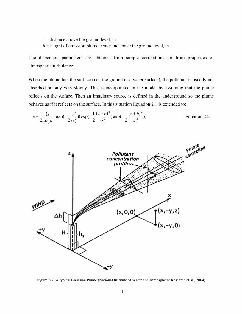
models to use. Figure 2-2 represents a simple Gaussian plume shape used in modeling.
The equation for pollutant concentration in the Gaussian plume model, in the absence of
boundaries, is as follows:
))(
2
1exp()
2
1exp(
2 2
2
2
2
zyzy
hzy
u
Qc
Equation 2.1
Where: c = concentration at given point, g/m3 Q = emission rate, g/s u = wind speed, m/s
σy = dispersion parameters in the horizontal (lateral) direction (depends on distance from the source), m σz = dispersion parameters in the vertical direction (depends on distance from the source), m
y = distance crosswind from the emission source, m
11
z = distance above the ground level, m h = height of emission plume centerline above the ground level, m
The dispersion parameters are obtained from simple correlations, or from properties of
atmospheric turbulence.
When the plume hits the surface (i.e., the ground or a water surface), the pollutant is usually not
absorbed or only very slowly. This is incorporated in the model by assuming that the plume
reflects on the surface. Then an imaginary source is defined in the underground so the plume
behaves as if it reflects on the surface. In this situation Equation 2.1 is extended to:
)))(
2
1exp()
)(
2
1)(exp(
2
1exp(
2 2
2
2
2
2
2
zzyzy
hzhzyQc
Equation 2.2
Figure 2-2: A typical Gaussian Plume (National Institute of Water and Atmospheric Research et al., 2004)

12
Generally, using Gaussian plume models are acceptable when (National Institute of Water and
Atmospheric Research et al., 2004):
Contaminants are unreactive chemically
Topographical condition is simple with no slopes
The meteorology does not vary much during small periods of time
There are few periods of calm or light wind
These factors make the Gaussian models convenient tools in the modeling:
They do not need an extensive numerical calculation - Gaussian models can be run on
almost all computers without necessarily having a good processor.
They are easy to use – they need only limited input data. They do not need complex
meteorological data.
They provide conservative results in the vicinity of the emission source.
They are widely used even today – well known with a wide variety of users and well
developed, so they are comparable between different studies.
AERMOD, CTDMPLUS, AUSPLUME, and ISCST3 are some examples of Gaussian air
dispersion models.
2.1.2 Advanced Dispersion Models
Though Gaussian plume models are widely accepted in air quality assessments and regulation,
sometimes more accurate and detailed results are desirable. Using more detailed data, advanced
air dispersion models provide more dependable, accurate, and realistic modeling results.
Advanced dispersion models perform more numerical calculations in order to run a simulation
and thanks to access to high performance computers, these models have become more common.
They can be categorized into three main groups based on the type of calculations; puff, particle,
and grid point. In puff models, pollutant releases are represented by a series of puffs of material.
Each puff represents a group of contaminant molecules whose volume increases due to turbulent
mixing and they are transported by the model wind. The puffs are assumed to have a Gaussian
concentration profile in three dimensions. Puff models are moderately expensive
computationally. In particle models, released pollutants are represented by a stream of particles
even if they are gas. In this type, pollutants are transported by the model wind and diffuse

13
randomly according to the model turbulence. Particle models are computationally more
expensive than puff models. In grid point modeling, contaminants distribution is shown by
concentration on a three-dimensional grid. This is the computationally most expensive type of
model and is usually used for airshed modeling (National Institute of Water and Atmospheric
Research et al., 2004).
Generally, the main difference between the Gaussian plume models and advanced dispersion
models is that the advanced models need more complicated (three dimensional) meteorological
information than the Gaussian plume models. The following are the situations where the
advanced models provide better results than Gaussian plume models (National Institute of Water
and Atmospheric Research et al., 2004).
Chemical reaction between pollutants and ambient air is important.
Appropriate and complete meteorological data is provided.
Meteorological condition varies in the modeled field, so steady state Gaussian models
cannot be applied.
Source or receptors are located in steep or complex terrain.
Pollutants accumulate in calm conditions or are re-circulated as the wind changes
direction.
Frequent periods of low wind speed are expected in the area.
Many modern atmospheric dispersion modeling programs contain pre and post-processor
modules. These pre and post processor modules improve user friendliness of the interface and
allow to input the meteorological, topographical and all other input data by pre-processor
modules. Graphical output data, and/or plots of the affected area by pollutants can be obtained
from post-processors modules.
The main example of advanced air dispersion models is the Gaussian puff model CALPUFF,
which is used widely in industries. In Alberta it is the preferred model for regulatory
applications.

14
2.2 CALPUFF
2.2.1 Background
Scire et al. (1990a, 1990b) developed a dispersion modeling system based on:
A meteorological modeling package with diagnostic wind field generator, and capability
of taking the results of a prognostic model (like MM5) as input data
A Gaussian puff dispersion model with chemical removal, wet and dry deposition,
complex terrain algorithm, building downwash, and plume fumigation
Post processing programs for output fields of meteorological data, concentration and
deposition fluxes
So, based on these components, considering the main needs in developing a new dispersion
model, CALPUFF was designed originally to deal with these objectives:
To treat time variable point and area sources
To predict concentrations with averaging times from one hour to one year
To deal with different modeling domains from tens of meters to hundreds of kilometers
To be used for inert pollutants and those subject to linear removal and chemical
conversion mechanisms
To be used for rough or complex terrain situations
Then CALPUFF, after integrating into the CALGRID model (a photochemical model) and the
Kinematic Simulation Particle (KSP) Model (a Lagrangian particle model, to complete the
modeling system for both reactive and non-reactive pollutants) became more comprehensive.
The Interagency Workshop on Air Quality Modeling (IWAQM) which consists of
representatives from the U.S. Environmental Protection Agency (EPA), U.S. Forest Service,
National Park Service, and U.S. Fish and Wildlife Service evaluated CALPUFF along with the
other models and indicated that using CALMET/CALPUFF models with MM4 data (four
dimensional meteorological data assimilation) could improve modeling performance over that of
other models. Then, the use of CALMET/CALPUFF to estimate air quality impact was
recommended by the IWAQM report (EPA, 1998) relative to the National Ambient Air Quality
Standards (NAAQS) and Prevention of Significant Deterioration (PSD) increments. Then EPA

15
has categorized the CALPUFF modeling system as a Guideline (“Appendix A”) model (see
Table 2-1) which should be used for the regulatory application involving long range transport,
and also, where non-steady-state effects may be important in a case-by-case basis for near-field
usage.
As a part of work for IWAQM, U.S. EPA, the U.S.D.A Forest Service, the Environmental
Protection Authority of Victoria (Australia), and the private industry in the U.S. and other
countries, the CALMET and CALPUFF models have been changed, revised, and improved many
times. The model has been made more appropriate for regional application, among other
enhancements.
2.2.2 Overview of the CALPUFF Modeling System
As mentioned before, dispersion models are categorized into three groups depending on the way
the air pollutants are represented by the model; Particles, Puffs, and Grid points. The CALPUFF
modeling system is one of the “Puff” models. CALMET, CALPUFF, and CALPOST are three
main components of the CALPUFF modeling system. Generally, CALMET is responsible for
meteorological processing. This model develops hourly wind speed and temperature values on a
three-dimensional gridded modeling domain. The CALPUFF model simulates dispersion and
transformation process. It uses gridded fields generated by CALMET, which are incorporated
throughout a simulation period to produce a distribution of puffs. Outputs of the dispersion
simulating step (CALPUFF model) contain either hourly concentrations or hourly deposition
fluxes calculated at receptors. Finally, CALPOST is used to process the output files generated by
CALPUFF to calculate average values, percentiles and extreme values, extinction coefficients
and related measures of visibility, and report these for each location. Figures 2-3 and 2-4 show
an overview of elements used in the CALMET/CALPUFF modeling system.

16
Figure 2-3: Overview of the program elements in the CALMET/CALPUFF modeling system (Scire et al., 2000)

17
Figure 2-4: Postprocessing: CALPOST/PRTMET postprocessing flow diagram (Scire et al., 2000)

18
2.2.3 Puff Model Formulation
There is a fundamental similarity between Gaussian puff and Gaussian plume models. The
mathematical description of a puff is based on the following equation:
zyxpQc Equation 2.3
Where: Qp = the emission contained in the puff, mg
In this equation �x and �y are defined in Lagrangian coordinates (i.e., in puff following
coordinates) as:
)2
1exp(
2
12
2
xxx
X
Equation 2.4
)2
1exp(
2
12
2
yyy
Y
Equation 2.5
And �z is defined in Eulerian coordinates (i.e., terrain following coordinates) assuming puff
reflection on the surface, as follows:
)])(
2
1exp()
)(
2
1[exp(
2
12
2
2
2
zzzx
hzhz
Equation 2.6
To be able to describe a finite plume as a series of puffs accurately, a large number of very dilute
puffs should be considered. This is the direct puff method for calculating the plume
concentration (De Visscher, 2013). For the direct puff method to be effective, each source should
emit at least one puff per second to resolve the plume near the source in some cases (Scire et al.,
2000a). To solve this weakness, it is possible to define extra puffs near the receptors (Zannetti,
1981), or to merge puffs far from the source that are more closely spaced than necessary
(Ludwig et al., 1977). The computational demands of these two improvements are still very
large. Hence, two integrated methods have been proposed. The first method is called integrated
puff method. It has been incorporated in MESOPUFF II (Scire et al., 1984a, b) and in
CALPUFF. And the second one, the slug method, has been incorporated in CALPUFF (Scire et
al., 2000). In these two methods some simplifying assumptions have been made to meet the

19
weakness of the direct puff method by using integrals to calculate the time-averaged
concentration of a moving plum.
Assuming that the receptor is at the coordinates (xr,yr) and the puff center moves from (x1,y1) to
(x1+Δx,y1+Δy), The final equation for the integrated puff method was offered as:
)]2
()2
()[22
exp(22
22
a
berf
a
baerf
c
a
b
a
Qc
xy
pavr
Equation 2.7
Where: 2
22 )()(
y
yxa
211 )()(
y
rr yyyxxxb
2
21
21 )()(
y
rr yyxxc
Based on this method, the number of puffs needed for calculating the concentration accurately is
reduced to one per hour (Scire et al., 2000a). This is the main equation which is implementing
the plume concentration calculation in CALPUFF.
2.2.4 CALPUFF Features and Options
“CALPUFF is multi-layer, multi-species non-steady-state puff dispersion model which can
simulate the effects of time-and space-varying meteorological conditions on pollutant transport,
transformation, and removal” (Scire et al., 2000). Input of CALPUFF can be either three
dimensional meteorological fields which are the output of the CALMET model, or just simply
the meteorological data used to drive the AUSPLUME (Lorimer, 1986), CTDMPLUS (Perry et
al., 1989), or ISCST3 (EPA, 1995) steady state Gaussian models.
CALPUFF also has many other options which include dealing with near-source effects like
building downwash, longer range effects like vertical wind shear, chemical transformation, and
over water transport. All the major features and options of the CALPUFF modeling system are
summarized in Table 2-2.

20
Table 2-2: Major Features of the CALPUFF Model (Scire et al., 2000)
Source type
Point source (constant or variable emissions)
Line source (source or variable emissions)
Volume sources (constant or variable emissions)
Area source (constant or variable emissions)
Non-steady-state emission and meteorological conditions
Gridded 3-D field of meteorological variables (winds, temperature)
Spatially-variable fields of mixing height, friction velocity, convective velocity scale,
Monin-Obukhov length, precipitation rate
Vertically and horizontally-varying turbulence and dispersion rates
Time-dependent source and emissions data
Efficient sampling function
Integrated puff formulation
Elongated puff (slug) formation
Dispersion coefficient (σy, σz) option
Direct measurements of σv and σw
Estimated values of σv and σw based on similarity theory
Pasquill-Gifford (PG) dispersion coefficient (rural areas)
McElroy-Poorler (MP) dispersion coefficients (urban areas)
CTDM dispersion coefficients (neutral/stable)
Vertical wind shear
Puff splitting
Differential advection and dispersion
Plume rise
Partial penetration
Buoyant and momentum rise
Stack tip coefficient
Vertical wind shear
Building downwash effects
Building downwash
Huber-Snyder method

21
Schulman-Scire method
Sub-grid scale complex terrain
Dividing streamline, Hd:
Above Hd, puff flows over the hill and experiences altered diffusion rates
Below Hd, puff deflects around the hill, split, and wraps around the hill
Interface to Emission Production Model (EPM)
Time-varying heat flux and emission from controlled burns and wildfires
Dry deposition
Gases and particulate matter
Three options:
Full treatment of space and time variations of deposition with a resistance model
User-specified diurnal cycles for each pollutant
No dry deposition
Overwater and coastal interaction effects
Overwater boundary layer parameters
Abrupt change in meteorological conditions, plume dispersion at coastal boundary
Plume fumigation
Option to introduce sub-grid scale Thermal Internal Boundary Layers (TIBLs) into
coastal grid cells
Chemical transformation options
Pseudo-first-order chemical mechanism for SO2, SO42-, NOx, HNO3, and NO3
-
(MESOPUFF II method)
User-specified diurnal cycles of transformation rates
No chemical conversion
Wet removal
Scavenging coefficient approach
Removal rate a function of precipitation intensity and precipitation type
Graphical user interface
Point-and-click model setup and data input
Enhanced error checking of model inputs
On-line Help files

22
2.3 Plume Modeling and Plume Rise
In many cases of dispersion modeling, the transport of diffusing material after release cannot be
considered as a passive phenomenon. Generally, the velocity and density of the released plume
may be different from those of the ambient air, so the released puff or plume might rise or fall
after being released from the stack. Therefore, for improving the modeling accuracy in these
cases, we need to understand the effects of initial momentum or buoyancy on the trajectory of
the plume or puff.
The different methodologies to model the plume rise can be divided into four main types; purely
empirical formulas, empirical formulas based on dimension analysis, simple formulas based on
material, heat, and momentum balance and finally equations based on Computational Fluid
Dynamics (CFD) expressing heat, mass, and momentum balance (De Visscher, 2009; Arya,
1999).
1- Purely empirical equations: purely empirical plume rise formulas are based on statistical
correlation and regression of observed plume rise with some relevant emission and
atmospheric variables. These equations are simple and easy to use, but cannot be applied
outside the range of conditions for which they have been tested (De Visscher, 2009).
Briggs (1969) has provided a brief review of early empirical relations for the rise of
buoyant plumes and momentum jets.
2- Equations based on dimension analysis: this method is also empirical, but based on dimension
analysis and similarity. Briggs (1968) applied this method to derive a model for the
plume rise for different source emissions and atmospheric conditions. These equations
are relatively simple and accurate, but because many different cases need to be identified
many different equations need to be used (De Visscher, 2009). Equations of this type are
summarized in section 2.3.1.
3- Simple momentum, energy, and mass balance equations: This type of plume rise model is based
on simple momentum, mass, and energy balances. All the equations are combined and
form a set of differential equations, and all the model needs is to solve them numerically
(De Visscher, 2009). This type is known as numerical plume rise model.

23
This dissertation is a study to extend the plume rise module PRIME (Plume Rise Model
Enhancements) to include flare combustion. The PRIME plume rise module was based
on Hoult and Weil’s (1972) work (Schulman et al., 2000), and is used in the CALPUFF
air dispersion model for simulating large buoyant area sources like forest fires (Scire et
al., 2000). Simple conservation equations allow this type of model to be used easily in
any air dispersion models (like CALPUFF), without requiring any extensive calculations.
4- Computational Fluid Dynamics (CFD): “Computational Fluid Dynamics (CFD) is in part, the
art of replacing the governing partial differential equations of fluid flow with numbers
and advancing these numbers in space and/or time to be obtain a final numerical
description of complete flow field of interest” (Wendt, 1992). CFD is part of fluid
mechanics, and uses numerical methods and algorithms to calculate and analyze
problems related to fluid flows like a moving plume in the ambient air. This method
involves the conservation of mass, momentum, and energy equations for buoyant plumes
and momentum jets. This type of model can be the most accurate one between these four
types of modeling, but it is the most intensive computationally. Since this method needs a
large amount of calculations, sometimes simulating the trajectory of a plume in a large
field, it requires super-fast computers with extensive memory space. Consequently, using
CFD to model plume rise in air dispersion models is not the most practical approach.
They are so computationally costly and time consuming, thus they are not appropriate for
a real time application. Despite their complexity, their results are not 100% reliable
(Argyropoulos, 2009).
The plume leaving the chimney from an industrial plant rises above the stack when it is either
warmer than the surrounding air, which results in lower density rather than ambient air
(buoyancy or thermal rise), or released at high velocity from the stack to give the exit gases
enough kinetic energy to move upward (momentum rise). The effect of the thermal rise is more
likely to have a dominant effect on the plume rise. Based on a rule of thumb, the buoyancy rise is
dominant if the exit gas temperature is 10-15 K more than ambient air (Turner, 1994).
Depending on the amount of turbulence in the surrounding air, the effect of buoyancy will be
diluted after 3-4 minutes when a sufficient volume of ambient air is entrained into the plume,

24
decreasing its temperature to that of the ambient air. Also, in 30-40 seconds the effects of the
momentum force will be degenerated (Turner, 1994).
Briggs (1965, 1968, 1969, 1972, and 1975) provided a set of plume rise equations based on
dimension analysis. These equations are widely accepted and have been adopted by U.S. EPA
and many others to be used in their stack gas dispersion models. A survey (1972) showed that
about 43% of organizations (not including EPA) involved in the stack plume dispersion
modeling in the U.S.A, Canada, and Japan were applying Briggs equations. Since the study, this
usage has been probably grown even wider globally (Beychok, 2005).
2.3.1 Briggs Equations
Briggs (1969) divided plumes into four general types:
1- Cold jet plumes in calm conditions
2- Cold jet plumes in windy conditions
3- Hot, buoyant plumes in calm conditions
4- Hot, buoyant plumes in windy conditions
Briggs assumed that the movements of cold jet plumes are dominated mainly by their initial
velocity momentum, however hot buoyant jet plumes are influenced more by their buoyancy
momentum. Even though Briggs provided plume equations for all types of plumes, “the Briggs
equations” which have become widely accepted are those for bent-over, hot buoyant plumes
(Beychok, 2005).
Briggs (1965) considered six variables to formulate the plume rise phenomenon:
Momentum flux parameter: 22ss
sm wrF
[m4/s2]
Buoyancy flux parameter: 221 sss
b wgrF
[m4/s3]
Stability parameter: dz
d
T
gs
[s-2]

25
Mean horizontal wind speed: u [m/s]
Time of travel: t [s]
Plume rise: Δz (transitional); Δh (final) [m]
Where: s = stack gas density, g/m3
= atmosphere air density, g/m3
rs = stack radius, m
sw = vertical velocity of stack gas, m/s
g = gravitational acceleration, m/s2
T = temperature of atmosphere, K
dz
d= potential temperature gradient
Transitional plume rise refers to the height Δz which a plume has risen by the time it reaches to
certain location, while final plume rise indicates the height Δh which a plume has risen by the
time it stops rising.
In a stable atmosphere, Briggs proposed the following equations to calculate the transitional
plume rise:
Buoyancy-dominated: 3
1
3
2bF
1.6z
u
x Equation 2.8
Momentum-dominated: 3
1
22
u
xFz m Equation 2.9
And for final plume rise:
Buoyancy-dominated: 3
1
bF2.6h
su Equation 2.10
Momentum-dominated: 3
1
215.1
su
Fh m Equation 2.11

26
Since these equations tend to infinity when wind speed is very low, the final plume rise for very
low wind speeds is changed to:
Buoyancy-dominated: 8
1
3bF
5.3h
s Equation 2.12
Momentum-dominated: 4
1
4.2
s
Fh m Equation 2.13
And when the atmosphere is near neutral (s=0) the above equations are replaced by:
Buoyancy-dominated: 3bF
004hu
Equation 2.14
Momentum-dominated: 2
3u
Fh m Equation 2.15
Where plume rise is influenced by both momentum and buoyancy, Briggs (1975) suggested the
following equation:
31
22
2
22 6.02
3
6.0
3
u
xF
u
xFz bm Equation 2.16
Arya (1999) summarized the above equation in Table 2-3.
Table 2-3: Plume rise prediction based on dimensional analysis (Arya, 1999)
Stability/Wind
Condition Type of Rise/Plume
Buoyancy-dominated
Plume
Momentum-dominated
Plume
Unstable and
neutral/windy Transitional/bent over
31
3
2bF
1.6z
u
x
31
22
u
xFz m
Stable/windy Final/bent over 3
1
bF2.6h
su
31
215.1
su
Fh m
Stable/calm Final vertical 8
1
3bF
5.3h
s
41
4.2
s
Fh m

27
Neutral/windy Final/bent over 3bF
004hu
2
3u
Fh m
2.3.2 CFD Formulation
Computational fluid dynamics (CFD) is a branch of fluid mechanics that uses numerical methods
and algorithms to solve and analyze problems that involve fluid flows. CFD applies numerical
models for the governing transport equations for mass, energy, species, and momentum, the
latter based on the Navier-Stokes equations. Because of the range of scales at which turbulent
motions exist, direct simulation of atmospheric dynamics is impossible in practice with current
computer technology. So, the smallest turbulence scales should be represented with some
empirical models as they cannot be resolved by direct simulation. The two main methods to
represent the smallest scales are Reynolds averaged Navier Stokes (RANS) and large eddy
simulation (LES).
The Navier-Stokes equations describe the momentum balance equation for fluids. The derivation
of the Navier-Stokes equations is based on Newton’s second law, considering the total force as
the sum of a gravity force Fg, a Coriolis force Fc, a pressure force Fp, and a viscous force Fs
which influence a fluid element with mass “m”. Hence:
spcg FFFFonacceleratim Equation 2.17
Equations 2-18, 2-19, and 2-20 are the Navier-Stokes equations describing an incompressible
Newtonian fluid.
2
2
2
2
2
21
z
u
y
u
x
u
x
pf
z
uw
y
uv
x
uu
t
u
Equation 2.18
2
2
2
2
2
21
zyxy
pfu
z
vw
y
vv
x
vu
t
v
Equation 2.19
2
2
2
2
2
21
z
w
y
w
x
w
z
pg
z
ww
y
wv
x
wu
t
w
Equation 2.20

28
Where: u, v, and w = winds speeds in x, y, and z directions, m/s
ν = kinetic viscosity, m2/s
ρ = density, kg/m3
p = pressure, Pa
f = Coriolis parameter (= 2 sin�, with the angular velocity of the earth, and � the
latitude)
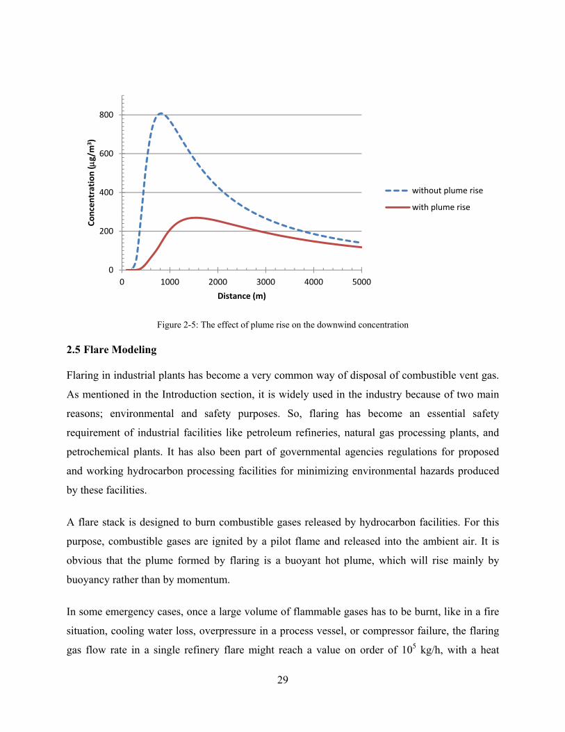
2.4 The Effect of Plume Rise on the Downwind Concentration
As an illustration of the importance of plume rise on the ground-level concentration downwind
of a source, an air dispersion calculation was made in the presence and in the absence of plume
rise. The source was assumed to have a stack height of 50 m, and a pollutant emission flow rate
of 50 g/s. The wind speed was assumed to be 3 m/s, ambient temperature 15 °C, plume
temperature 65 °C. The stack radius is 37.5 cm (i.e., diameter 75 cm), and the emission flow
velocity of the stack gas is assumed to be 5 m/s. Based on these data, a buoyancy flux parameter
of 5.1 m4/s3 is obtained. Plume rise is calculated with the equations in Table 2-3 assuming near-
neutral atmosphere.
The result of the calculations is shown in Figure 2-5. In the absence of plume rise, a ground-level
concentration of up to 800 µg/m3 can be expected, whereas plume rise lowers the maximum
ground-level concentration to 270 µg/m3. Clearly, accurate evaluation of plume rise is essential
for the accurate estimation of the environmental impact of industrial emissions.
29
Figure 2-5: The effect of plume rise on the downwind concentration
2.5 Flare Modeling
Flaring in industrial plants has become a very common way of disposal of combustible vent gas.
As mentioned in the Introduction section, it is widely used in the industry because of two main
reasons; environmental and safety purposes. So, flaring has become an essential safety
requirement of industrial facilities like petroleum refineries, natural gas processing plants, and
petrochemical plants. It has also been part of governmental agencies regulations for proposed
and working hydrocarbon processing facilities for minimizing environmental hazards produced
by these facilities.
A flare stack is designed to burn combustible gases released by hydrocarbon facilities. For this
purpose, combustible gases are ignited by a pilot flame and released into the ambient air. It is
obvious that the plume formed by flaring is a buoyant hot plume, which will rise mainly by
buoyancy rather than by momentum.
In some emergency cases, once a large volume of flammable gases has to be burnt, like in a fire
situation, cooling water loss, overpressure in a process vessel, or compressor failure, the flaring
gas flow rate in a single refinery flare might reach a value on order of 105 kg/h, with a heat
0
200
400
600
800
0 1000 2000 3000 4000 5000
Conc
entr
atio
n (
g/m
3 )
Distance (m)
without plume rise
with plume rise

30
release rate of the order of 1000 MW for a few minutes. This shows the importance of safe
disposal of large quantities of unwanted flammable gases in the oil industry. The influence of the
ambient wind speed on the flare, its radiation field and the amount of radiation energy emitted
from the flare, noise problems, the efficiency of the flare for burning any toxic gases, and the
formation and dispersion of smoke and gaseous pollutants are subjects of studies by combustion
scientists (Bruzustowski, 1976).
In this dissertation, a numerical study has been done to model the flare combustion and flare
plume rise to be included in the air dispersion models like CALPUFF. CALPUFF includes a
module that is currently used for plume rise and dispersion modeling for large area source, which
is based on the work of Hoult and Weil (1972). This plume module does not include a flare
modeling section. In other words, PRIME cannot predict the plume rise from flare combustion,
or it does not allow for chemical reaction or heat production in the plume (De Visscher, 2009).
Hence, an additional set of equations is needed for predicting the flare combustion in CALPUFF.
To model plume rise from flare combustion, the current practice is to use simple empirical
equations to predict the flare size and orientation and the amount of air entrained into the flame.
Based on these calculations, a “theoretical” source is defined located at the flame tip.
There are several equations describing the size of flames in the literature. Kalghatgi (1983) fitted
empirical curves to a wind tunnel data set concerning the shape and size of turbulent
hydrocarbon jet diffusion flames in a cross wind. He found that both flame height (hf) and angles
of flame to the vertical (αB) were function of the ratio of wind speed to the stack exit speed (R).
His derived empirical relations are:
)2035.26()( 2
1
RRmm
Dh
af
Equation 2.21
RRB 35)6.1(94 Equation 2.22
Where: ma, m = molecular weights of air and flare gas, g/mol

31
Do = stack diameter, m
Beychok (2005) provides a set of equations predicting these features. In the Beychok flare model
an American Petroleum Institute (1969) publication is used to describe the flame length as
below:
478.0006.0 cQL Equation 2.23
Where: L= flame length defined as length of the visible flame, ft
Qc= flare gas heat release, Btu/hr
And for calculating the height of a flare stack flame, Beychok simply assumed that the angle of
flame from the vertical is 45°. Hence, using the previous equation:
478.00042.0
707.0)45(sin
cfv
fv
Qh
LLh
Equation 2.24
Where: hfv=vertical height of the flame
Steward (1978) published a study on flare size and developed a theoretical mathematical model
for turbulent diffusion flames as follows:
2.0218.16 NR
L
Equation 2.25
Where: L = flame length, ft R = stack exit radius, ft
N = a combustion parameter = ])1()(/[])/([ 522522 wgNHVRwrQ aac
r = stoichiometric air: fuel ratio, lb air/lb of flared gas w = a combustion parameter = )//()( NHVTrcTrc apap
NHV = flare gas net heating value, Btu/ft3 g = gravitational constant of 417*106ft/hr2
a = ambient air density, lbm/ft3
= fuel density, lbm/ft3
Ta = air temperature, °R cp = specific heat of air of 0.24 Btu/lbm/°F Qc = flared gas heat release, Btu/hr
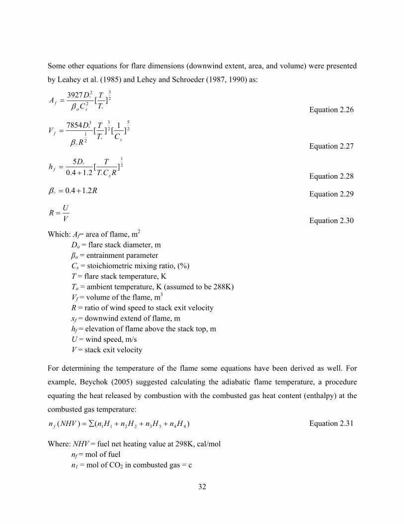
32
Some other equations for flare dimensions (downwind extent, area, and volume) were presented
by Leahey et al. (1985) and Lehey and Schroeder (1987, 1990) as:
2
3
2
2
][3927
T
T
C
DA
sf
Equation 2.26
2
5
2
3
2
1
3
]1
[][7854
sf CT
T
R
DV
Equation 2.27
2
1
][2.14.0
5
RCT
TDh
sf
Equation 2.28
R2.14.0 Equation 2.29
V
UR
Equation 2.30
Which: Af= area of flame, m2 Do = flare stack diameter, m βo = entrainment parameter Cs = stoichiometric mixing ratio, (%) T = flare stack temperature, K To = ambient temperature, K (assumed to be 288K) Vf = volume of the flame, m3
R = ratio of wind speed to stack exit velocity xf = downwind extend of flame, m hf = elevation of flame above the stack top, m U = wind speed, m/s V = stack exit velocity
For determining the temperature of the flame some equations have been derived as well. For
example, Beychok (2005) suggested calculating the adiabatic flame temperature, a procedure
equating the heat released by combustion with the combusted gas heat content (enthalpy) at the
combusted gas temperature:
)()( 44332211 HnHnHnHnNHVn f Equation 2.31
Where: NHV = fuel net heating value at 298K, cal/mol nf = mol of fuel n1 = mol of CO2 in combusted gas = c

33
n2 = mol of H2O in combusted gas = 0.5h n3 = mol of N2 in combusted gas = (1+x)(3.76)(c+.025h) n4 = mol of O2 in combusted gas = x(c+0.25h) c = carbon atoms per mole of fuel h = hydrogen atoms per mole of fuel x = (% excess air)/100
H1,H2,H3,H4 = enthalpies in cal/mol for the CO2, H2O, N2, and O2 in the combusted gas at the gas temperature T in K
In regards to these expressions for the specific combustion gas components:
5.2522)1028.0()1065.2(70.7 3623
2 TTTHCO Equation 2.32
2468)10447.0()10075.0(22.8 3623
2 TTTH OH Equation 2.33
7.2042)10043.0()10305.0(76.6 3623
2 TTTHN Equation 2.34
3107)1088.1()1013.0(27.8 1523
2 TTTHO Equation 2.35
Where: H = cal/mol of heat content above 298K T = combusted gas temperature, K
The combusted gas temperature can be calculated by trial-and-error selection of the temperature
which satisfies both sets of equations above.
The factors which influence the size of the flame include: diameter of stack, height of stack,
ambient air velocity, exit stack gas velocity, type of fuel, heating value of fuel, the heat loss by
radiation, etc. As mentioned before, none of these equations incorporate all these influencing
factors of the flame size of a flare.
Other than empirical equations, models based on computational fluid dynamics are another
common approach for flare modeling. Fairweather et al. (1991) applied a finite-difference
procedure to solve the flow equations to model the flare characteristics. In this study, length,
trajectory, and temperature profile of the flame are investigated by solving the full three-
dimensional forms of the partial differential conservation equations for mass, momentum, and
scalar transport. Hernandez et al. (1995) and Lawal et al. (2010) also offered some flare models
using a finite-volume procedure for solving the flow equations based on general assumptions
similar to those employed by Fairweather et al. (1991). The flow field of all these studies are

34
based on Reynolds Averaged Navier Stokes (RANS) equations. Smith et al. (2009) presented
another flare model using Large Eddy Simulation (LES) method to study the impact of H2S on
carbon and sulfur combustion.
When flare modeling is based on computational fluid dynamics, it is possible to incorporate all
those influencing factors, but the problem in using them is that they are too sophisticated and
need excess computational work, which make them almost impossible to be embedded into
current air dispersion models to be used for real time application. So, more simple equations and
solutions are needed to decrease the amount of computational work in air dispersion models.
In this study which is based on previous work of De Visscher (2009), a comprehensive set of
equations has been derived to describe flares, incorporating all the factors that influence the
flame size of the flare. Moreover, the solution procedure is easy enough to be included in air
dispersion models like CALPUFF.
Since this model is a numerical solution of some ODEs (Ordinary Differential Equations) for
describing the flame size, it can easily be embedded into the dispersion simulation software such
as CALPUFF compared to other sophisticated models.

3.1 Intro
PRIME
develope
used in C
third typ
for the c
equations
In the ori
a numeri
predict fl
by keepi
more diff
was fit to
mass ba
througho
The main
(2009) b
specific
results w
enhancem
Nine ord
are then
calculate
because v
the x and
distance
Visscher
Chapter T
oduction
(Plume Rise
ed for plume
CALPUFF to
e of models
conservation
s numericall
iginal model
cal solution
lare characte
ng track of
fferential equ
o flame leng
lance were
out the flare a
n purpose o
by optimizin
heat of amb
with real m
ments make
dinary differe
n solved sim
s the plume
variables tha
d z direction
traveled by
, 2009).
BasicThree:
e Model En
e rise and bu
o predict plu
s mentioned
of mass, m
ly leads to pr
l, 6 different
of the mass
eristics, so D
the amount
uations to PR
th correlatio
not optima
and plume, d
of this chap
ng the entrai
bient air. Th
measured fie
the model m
ential equatio
multaneously
e as a three
at define the
, and plume
y the plume
Model – Co
nhancements
uilding dow
ume rise fro
in Section 2
momentum, a
redictions of
tial equation
, energy, and
De Visscher (
of oxygen
RIME to be
ons, but not t
al, and the
despite a 200
ter is to im
inment facto
he entrainm
eld data fro
more realistic
ons will be d
y along wi
dimensiona
e plume as a
radius, are c
e. It is assu
35
onsidering i
s) is a popu
wnwash (Sch
om large are
2.3, which c
and energy.
f the trajecto
ns are respon
d momentum
(2009) exten
mixed into
able to acco
to real data.
specific he
00°C temper
mprove the f
ors, and usin
ent factors
om literatur
c.
developed ba
ith some au
al object, it
a three-dimen
calculated as
umed that th
instantaneo
ular plume
hulman et al
a sources. P
consists of a
Solving thi
ory of a plum
nsible for pr
m conservati
nded PRIME
the plume.
ount for the f
Moreover, t
eat of ambi
rature range.
flare combu
ng temperat
are optimiz
re instead o
ased on the c
uxiliary equ
is essentiall
nsional obje
s dependent
he plume c
ous reaction
rise model
l., 2000). Th
PRIME is an
a set of diffe
s set of ord
me.
edicting the
ion laws. PR
E to include
De Visscher
flare combus
the entrainm
ient air was
.
stion model
ture depende
ed by comp
of with cor
conservation
uations. Tho
ly a one-dim
ect, like plum
variables of
cross-section
n
which has
his model is
n example o
erential equa
dinary differe
plume rise u
RIME is unab
flare combu
r (2009) add
stion. This m
ment factors i
s taken con
l of De Vis
ent values o
paring the m
rrelations. T
n equations.
ough the m
mensional m
me location a
f “s” which
n is circular
been
s also
of the
ations
ential
using
ble to
ustion
ded 3
model
in the
nstant
sscher
of the
model
These
They
model
model,
along
is the
r (De

36
3.2 Model Development
The first step in this study is to obtain the differential equations describing the plume and flare
behavior. The equations of the numerical plume rise model PRIME will be adopted, and
extended to include flare combustion. Figure 3-1 below shows some variables in this numerical
model and a schematic of the plume considered by the model.
Figure 3-1: Schematic of the numerical plume rise model in CALPUFF (Scire et al., 2000)
PRIME includes the Equations 3.1 to 3.14 below.
The first equation is a mass balance for the rising plume. Based on this equation, the entrainment
of ambient air into the plume during the plume trajectory “s” increases the mass of the plume
while it is rising.

37
)sin2()cos2()( 2 atmatmatmscatmsc UrUUrrUds
d Equation 3.1
Where: s = path length of plume centerline measured from the emission source, m ρ = plume density, kg/m3 Usc = velocity of plume centerline, m/s r = radius of plume, m ρatm = density of atmosphere, kg/m3 Uatm = wind speed, m/s
ø = centerline inclination, angle between plume path and the horizontal in the wind direction, degrees α = plume entrainment parameter corresponding to velocity difference between plume centerline and wind in the parallel direction of the plume centerline = 0.11 β = plume entrainment parameter corresponding to velocity difference between plume centerline and wind in the normal direction of the plume centerline = 0.6
According to this equation there are two driving forces for entrainment of ambient air into the
plume: shear along the plume ( cosatmsc UU ) and shear across the plume ( sinatmU ). In the
left hand side of Equation 3.1, “ 2rUsc ” describes the mass of plume per unit of length, divided
by π. From Equation 3.1, the parameter “ 2rUsc ” forms the first dependent variable of the
model. All the equations in this model have been divided by π to simplify the equations.
To find differential equations relating the velocities of the plume and of ambient air, we need to
distinguish between the vertical and horizontal components of plume velocity. If we consider
“u” and “w” as the horizontal and vertical components of the plume velocity respectively, we
have:
u
dt
dx Equation 3.2
wdt
dz Equation 3.3
scUdt
ds Equation 3.4
Therefore, the second and third differential equations are derived from dividing Equations 3.2
and 3.3 by Equation 3.4:

38
cosscU
u
ds
dx Equation 3.5
sinscU
w
ds
dz Equation 3.6
In addition, “Usc” can be calculated from “u” and “w” as below:
22 wuUsc Equation 3.7
The fourth differential equation is the momentum balance in the wind direction. The frame of
reference chosen for momentum is the ambient wind. Hence, in this equation ambient air has no
momentum, so the momentum of the plume is not changed by adding air into the plume. In other
words, the momentum is calculated using the moving ambient air as an observer. Furthermore, it
is assumed that all the air that experiences friction from the passing plume is entrained into the
plume. Therefore, the only mechanism to change the momentum of the plume relative to the
ambient air is the velocity gradient of the ambient air itself:
dz
dUwrUurU
ds
d atmatmsc 22 ))(( Equation 3.8
Where: u = horizontal component of the plume speed, m/s w = vertical component of the plume speed, m/s z = height, m
The right hand side in this equation is related to wind shear, and the minus sign here means that
the plume loses momentum by moving up into faster moving air layers.
The momentum balance equation for the vertical direction holds the same principle, but the
assumption of zero vertical wind speed is taken, like in Equation 3.1. Hence, the difference
between the gravitational and buoyant force is the generator of the vertical momentum change.
The fifth differential equation is as follows:
)()( 22 atmsc grwrUds
d Equation 3.9
Where: g = gravitational acceleration, m/s2

39
As with momentum, the enthalpy of the plume is taken relative to the enthalpy of ambient air.
Hence, ambient air has zero enthalpy and does not affect the enthalpy of the plume when
entrained into the plume. On the other hand, plume rise can have an effect on the enthalpy of the
plume if the temperature changes due to plume rise differs from the temperature gradient (or
lapse rate) of ambient air. Hence, the energy conservation equation can be written as:
222 ))(( rc
Q
dz
dwrTTrU
ds
d
p
atmatmsc
Equation 3.10
Where: T = temperature of flare, K Tatm = temperature of ambient air, K
cp = specific heat of air, kJ/kg K Q = radiative heat loss per unit volume of the plume, (kJ/m3)
dz
d atm
= lapse rate of ambient potential temperature which can be calculated as below:
p
atmatm
c
g
dz
dT
dz
d
Equation 3.11
Where dz
dTatm is the temperature gradient of ambient air (negative when the temperature declines
with increasing height), and pc
g is the adiabatic lapse rate of a rising plume, i.e. the temperature
change of the plume per meter of plume rise in adiabatic conditions. The adiabatic lapse rate is
derived from thermodynamic principles in Appendix A.
The specific heat of air is obtained from the following formulation (Sandler, 1999) for the range
of 273-2800 kelvin:
32-5-2p T1.965 - T100.48 + T100.197 + 28.088=c Equation 3.12
Where cp is in J/mol K, and T is in K.
The last term describes the radiative heat loss from the plume to the ambient air. This term is
important only initially when the plume temperature is high, and in the presence of combustion.
Q in Equation 3.10 is the radiative heat loss per unit volume of the plume. It can be estimated as:

40
patmp
cTTrrc
Q/)(2 442 Equation 3.13
Where: ε = emissivity of the plume σ = Stefan-Boltzman constant = 5.76*10-11 kJ/s m2 K4
Schulman et al. (2000) proposed a value of 0.8 for ε for plume rise from large area sources.
However, 0.8 is relatively high for small plumes.
Substituting Equations 3.11 and 3.13 into Equation 3.14, the last differential equation is obtained
for the energy balance:
)(2
)())(( 4422atm
pp
atmatmsc TTr
cc
g
dz
dTwrTTrU
ds
d
Equation 3.14
The term )))((( 2atmsc TTrU
ds
d is the enthalpy change. In this equation it is equal to the sum of
the heat the plume loses from radiation ( )(2 44
atmp
TTrc
) and the change of enthalpy due to
changes of the ambient air potential temperature ))(( 2
p
atm
c
g
dz
dTwr with respect to the height.
The lapse rate term which shows the altitude dependence of temperature is discussed in
Appendix A.
Hence, we have six independent differential equations and six independent variables. All these
differential equations are included in the PRIME plume rise model, and describe plume rise from
large area sources like forest fires. To include flare combustion, we need to add some additional
differential equations relating to the flare effects as well. De Visscher (2009) added four more
ordinary differential equations to be solved along with the original equations to describe flare
combustion.
First, De Visscher (2009) assumed complete mixing and instantaneous reaction in the flare. Then
he calculated conversion of combustion X, by assuming that the amount of oxygen reacted with
methane equals the amount of oxygen mixed into the plume:

41
n
m
rU
rUrUX O
ssc
sscsc 2
02
022
)(
)(
Equation 3.15
Where: 2Om = mass fraction of oxygen in the air
n = stoichiometric factor, kg oxygen consumed per kg fuel combusted
In Equation 3.15, term 02 )( sscrU is the mass flow rate of initial fuel (pure methane) in the stack
tip and2
))(( 022
Osscsc mrUrU relates the mass flow rate of oxygen entering into the plume.
To get a differential equation, the derivative with respect to “ds” is taken:
)()(
2
02
2 rUds
d
rUn
m
ds
dXsc
ssc
O
Equation 3.16
When the conversion of combustion reaches to 1 (X=1), it means that the entire combustible
plume has been burned. In other words, it leads us to the end point of the flame. Therefore, the
“s” amount related to “X=1”, shows the tip of the flare flame.
Solving all these equations yields dimensions of the flare, but these equations result in
unrealistically short flames. The reason is the assumption of complete mixing during the plume.
Complete mixing assumes that all the oxygen mixed into the plume has been reacted with the
fuel and leads to flames that are unrealistically short. Therefore, it is assumed that mixing is
incomplete and just part of the air mixed into the plume enters the burning section of the plume.
Hence, the flame is subdivided to a burning mass fraction “f” and a non-burning mass fraction
“1-f”. Assuming that a constant portion of the air mixed into the plume, “fmix”, enters the burning
section leads to extra mass and heat balance equations:
)()( 22 rUds
dfrUf
ds
dscmixsc Equation 3.17
)(2
)()())(( 4420
22atmf
pp
atm
psscatmfsc TTf
cwr
c
g
dz
dTf
ds
dX
c
HrUTTrUf
ds
d
Equation 3.18
22 ))(1())()1(( wrc
g
dz
dTfTTrUf
ds
d
p
atmatmairsc Equation 3.19

42
Where H is the enthalpy of combustion in kJ/mol. Equation 3.18 is the heat balance for the
burning section of flame and Equation 3.19 relates to the non-burning part of the flame.
De Visscher (2009) suggested a value of 0.0293 for “fmix” to be concluded in the heat balance
equations. This value was based on a model fit to empirical flame length equations.
Therefore, adding Equations 3.16 and 3.17 to the set of independent differential equations and
substituting Equation 3.14 by 3.18 and 3.19 leads to nine independent differential equations
describing characteristics of the flare.
3.2.1 Emissivity Calculation
Calculating an acceptable value for the emissivity plays an important role in flare modeling since
it has a direct effect on the heat balance equations (Equation 3.18 and 3.19). Schulman et al.
(2000) suggested a value of 0.8 for the emissivity of large area sources like forest fires. As large
area sources are much bigger than flares, this emissivity is much higher than what is expected for
flares, thus a different approach is required to obtain the flare emissivity.
Beychok (2005) suggested that 25% of the heat produced by combusted gas is lost by radiation at
the end of the visible flame which is a conservative assumption that is not exceeded in practical
conditions. Accordingly, to calculate the emissivity, we need to know the type of hydrocarbon
burned in the stack and then determine the heating value of the gas. Thus, setting the percentage
of heat loss by radiation to the amount of 25%, leads to an appropriate emissivity prediction.
A fraction of radiation heat loss occurs past the flame tip. Hence, it is evaluated at
length" flame"2s because radiation is negligible past that point. The heat loss due to
radiation is calculated with the following differential equation (De Visscher, 2009):
HrU
cTT
c
r
ds
lossradiationd
ssc
patmf
p 02
44
)(
)(2)(
Equation 3.20
Where: ε= emissivity of flare H = heat of combustion, J/kg

43
All the independent differential equations along with independent variables are summarized in
Table 3-1.
Table 3-1: Independent differential equations along with their independent variables
# Differential Equation Variable
1 )sin2()cos2()( 2 atmatmatmscatmsc UrUUrrUds
d 2rUsc
2 cosscU
u
ds
dx x
3 sinscU
w
ds
dz z
4 dz
dUwrUurU
ds
d atmatmsc 22 ))(( )(2
atmsc UurU
5 )()( 22 atmsc grwrUds
d wrUsc
2
6 )(*)(
2
02
2 rUds
d
rUn
m
ds
dXsc
ssc
O
X
7 )()( 22 rUds
dfrUf
ds
dscmixsc 2rUf sc
8
)(2
)(
)())((
442
022
atmfpp
atm
psscatmfsc
TTfc
wrc
g
dz
dTf
ds
dX
c
HrUTTrUf
ds
d
)(2atmfsc TTrUf
9 22 ))(1())()1(( wr
c
g
dz
dTfTTrUf
ds
d
p
atmatmairsc
)()1( 2
atmairsc TTrUf
10 HrU
cTT
c
r
ds
lossradiationd
ssc
patmf
p 02
44
)(
)(2)(
Radiation-loss
3.3 Results and Discussion
To calculate the dimensions of the flame, all the independent differential equations in Table 3-1
are solved in MATLAB. Based on initial conditions of the stack and meteorological situations,

44
the results change. Hence, to compare the results with observational data collected in the field,
we need to set some parameters to correspond to the observational tests conditions. The
parameters which are influenced by the stack and meteorological conditions include:
1- Heating value of fuel (kJ/kg fuel)
2- Heat of combustion (Watt)
3- Stoichiometric factor (in the study of pure methane its value equals 4)
4- Gas exit velocity (m/s)
5- Wind speed (m/s)
6- Atmosphere temperature (K)
7- Gas temperature (K)
8- Atmospheric entrainment parameters (m)
Along with all these parameters, it is assumed that the atmosphere is adiabatic (p
atm
c
g
dz
dT )
with a ground-level temperature of 15oC.
Leahey et al. (1987) collected some observed data of flame length and orientation of a flare,
which is shown in Table 3-2 and 3-3. So, to compare these field data with modeling results we
need to set all the stack influencing factors and ambient wind speed in the modeling codes as
Table 3-2.
Table 3-2: Flare stack parameters for indicated test time (Leahey et al., 1987)
Tes
t
Time
(MST)
Acid
Gas
(m3h-1)
Fuel
Gas
(m3h-1)
Molecular
Weight
(g mol-1)
Flame
Temperature
(K)
Heat
Content
(MJ m-3)
Exit
Speed
(m s-1)
Wind
Speed
(m s-1)
March 7
1 20:02-20:04 124 77 34.3 1353 17.6 7.6 1.3
2 20:16-20:18 126 60 35.6 1323 15.5 7.1 1.4
3 20:33-20:34 122 38 37.4 1213 12.5 6.1 1.4
March 8
4 21:50-21:51 131 92 33.6 1273 18.6 8.5 2.8
5 21:56-21:57 124 49 36.5 1103 14.0 6.7 3.2

45
6 22:07-22:08 122 28 38.5 1073 10.7 5.8 3.0
7 22:25-22:26 122 0 42.8 673 4.1 4.6 3.2
8 22:33-22:34 122 16 38.1 823 8.1 5.3 2.8
Table 3-3: Observed values of hf/D and angle (Leahey et al., 1987) Test hf/D αB
1 10±3 54±6
2 10±2 51±8
3 8±1 53±5
4 9±3 64±10
5 4±0 73±2
6 4±2 72±10
7 2±1 68±12
8 2±2 70±11
Leahey et al. (1987) compared two flare variables: height of the flare divided by diameter of the
stack ( Dh f / ) and angle of the flare to the vertical (αB).
To run the model based on these input parameters, it is necessary to calculate the appropriate
value for mixf . Choosing proper value for mixf is of prime importance for this part of study, since
a small change in mixf value leads to significant errors in calculating the flame characteristics.
For the first step mixf is set for each data point to meet the results in Table 3-3. Hence, running
the model for the initial conditions of observational data leads to the results offered in Table 3-4.
Table 3-4: Predicted values of hf/D and angle hf/D αB (degree)
Test mixf observed predicted observed Predicted
1 0.06 10±3 10.18 54±6 32
2 0.085 10±2 10.25 51±8 37

46
3 0.13 8±1 8 53±5 38
4 0.065 9±3 8.9 64±10 60
5 0.33 4±0 4 73±2 68
6 0.25 4±2 4 72±10 62
7 0.9 2±1 3 68±12 68
8 0.55 2±2 3 70±11 68
Table 3-4 shows the observed and predicted values for the height and angle of the flare. It shows
that the theory tended to underestimate αB and in some tests overestimated the height of the flare.
This is related to the values of the entrainment factors. As discussed before in the model
development section, α and β are the empirical parameters describing entrainment of the air into
the plume corresponding to the difference of wind and plume speed in both directions. Scire et
al. (2000) suggested a value of 0.11 and 0.6 for α and β, respectively, for area source plume rise.
Subsequently, using an entrainment factor for large area sources in a model for industrial stack
plumes, which are relatively small sources, has led to inaccuracies.
Since area sources, such as forest fires, are very large, the entrainment of some amount of
ambient air into that huge volume has less influence on plume rise than the entrainment of
ambient air into the relatively small and narrow industrial stack plume. In other words, on
account of the fact that the proportion of “volume of ambient air entering into the plume” to the
“initial volume of the plume” for the large area source is less than the industrial stack, ambient
air entering the plume has more influence on the industrial stack plume rise than on large area
source plume rise. Hence, the entrainment rate of atmospheric air into the industrial stack plume
needs to be modified in this study.
Leahey et al. (1987) defined entrainment factor β as:
21
00 )( Equation 3.21
Where: β0=entrainment factor for a jet of density ρ0, m
ρ0=density of surrounding air, kg/m3

47
ρ=density of a jet, kg/m3
Which, according to Briggs (1975):
sc
atm
U
U2.14.00 Equation 3.22
However, Briggs did not offer any formulation for the factor defining entrainment of
atmospheric air parallel to the plume trajectory (α). Using Equation 3.22 instead of a constant
value of β=0.6 did not improve the agreement between the model and the data.
It is assumed that the proportion of α/β of a large area source is the same as for a flare. In view of
the fact that Leahey (1987) neglected the effect of α in the flare trajectory, we just manipulate the
amount of α and β suggested by Scire et al. (2000) to fit the observed data. A correction factor of
1.6 provided the best agreement with the measurement data. Hence, the modified entrainment
factors are:
αnew= 1.6 α
βnew= 1.6 β
Considering the new values for entrainment factors, predictions from the model are compared
with the observed data collected in the field in Table 3-5.
Table 3-5: Observed and predicted values of hf/D and angle (including modified entrainment factors: α and β) hf/D αB (degree)
Test mixf observed Predicted Observed Predicted
1 0.07 10±3 10.9 54±6 45
2 0.085 10±2 10.1 51±8 49
3 0.13 8±1 8.39 53±5 51
4 0.065 9±3 7.54 64±10 68
5 0.33 4±0 3.36 73±2 75
6 0.25 4±2 4.26 72±10 70.1
7 0.9 2±1 2.1 68±12 70.1
8 0.55 2±2 2.7 70±11 65

48
Figure 3-2: Observed and predicted values of hf/D (including modified entrainment factors)
Figure 3-3: Observed and predicted angel of the flare to the vertical (including modified entrainment factors)
Values of observed hf/D and αB were compared to the predicted values in Figures 3-2 and 3-3.
Predicted and observed values for each of the tests are also shown in Table 3-5. However, the
results from test 4 seem to deviate from other results. Even in the model which is offered by the
original study of Leahey et al. (1987) there is a considerable error for predicting the flare height
R² = 0.954
0123456789
101112
0 1 2 3 4 5 6 7 8 9 10 11 12
Pred
icte
d He
ight
of t
he F
lam
e/Di
amet
er
Of T
he S
tack
Measured Height Of The Flame/Diameter Of The Stack
hf/D
R² = 0.8593
40
45
50
55
60
65
70
75
80
40 45 50 55 60 65 70 75 80
Pred
icte
d An
gle
Of T
he F
lare
To
The
Vert
ical
(deg
ree)
Measured Angle Of The Flare To The Vertical (degree)
angle

49
and angle regarding this test. It may be the result of of some inaccuracies in the measurements
for this test. It is observed that the coefficient of determination (R2) for Figure 3-2 would
increase up to 0.983 (R2=0.983) and for Figure 3-3 up to 0.881 (R2=0.881) if the result of test 4
were omitted from the data set.
3.3.1 fmix Calculation
In general, wind speed and stack exit speed are the main parameters influencing mixf . To study
their effects, Figure 3-4 is shown. Note that for the sake of simplicity, the proportion of the wind
to stack exit speed is shown in this figure.
Figure 3-4: fmix vs. proportion of the wind speed to the stack exit velocity
As shown in Figure 3-4, mixf is directly correlated with the proportion of the atmosphere wind
speed to the stack exit speed (0)( ssc
atm
U
U). The bigger the proportion of the wind to the stack exit
speed, the bigger mixf . To model mixf , different-structured equations were fitted to the
experimental data shown in Figure 3-4 by regression to obtain the best equation for each
structure. After comparing all the equations, the following exponential equation is found to yield
the most accurate results:
y = 0.0362e4.5679x
R² = 0.9359
00.10.20.30.40.50.60.70.80.9
1
0 0.2 0.4 0.6 0.8
fmix
Wind speed/Stack speed

50
))(
5679.4exp(0362.00
ssc
atmmix U
Uf
Height and angle of the flare are predicted using this proposed equation, and the results are given
in Table 3-6 and Figures 3-5 and 3-6.
Table 3-6: Observed and predicted values of hf/D and angle (including modified entrainment factors: α and β, and formulated fmix)
hf/D αB (degree)
Test mixf observed Predicted Observed Predicted
1 0.0791 10±3 10.1 54±6 44
2 0.0911 10±2 9.8 51±8 49
3 0.1054 8±1 9.7 53±5 53
4 0.1653 9±3 3.9 64±10 60
5 0.3208 4±0 3.4 73±2 75
6 0.3851 4±2 2.8 72±10 66
7 0.86 2±1 2.1 68±12 71
8 0.4048 2±2 3.4 70±11 68
Figure 3-5: Observed and predicted values of hf/D (including modified entrainment factors and formulated fmix)
R² = 0.6673
0123456789
101112
0 1 2 3 4 5 6 7 8 9 10 11 12
Pred
icte
d He
ight
of t
he F
lam
e/Di
amet
er
Of T
he S
tack
Measured Height Of The Flame/Diameter Of The Stack
hf/D

51
Figure 3-6: Observed and predicted values of angel of the flare to the vertical (including modified entrainment
factors and formulated fmix)
As mentioned before, test 4 in this set of observed data seems to deviate from other observation
results. Ignoring the results of test 4 leads to the following comparison between predicted and
observed values in Figures 3-7 and 3-8.
Figure 3-7: Observed and predicted values of hf/D (including modified entrainment factors and formulated fmix)
R² = 0.8675
40
45
50
55
60
65
70
75
80
40 45 50 55 60 65 70 75 80
Pred
icte
d An
gle
Of T
he F
lare
To
The
Vert
ical
(deg
ree)
Measured Angle Of The Flare To The Vertical (degree)
Angle
R² = 0.9274
0123456789
101112
0 1 2 3 4 5 6 7 8 9 10 11 12
Pred
icte
d He
ight
of t
he F
lam
e/Di
amet
er
Of T
he S
tack
Measured Height Of The Flame/Diameter Of The Stack
hf/D

52
Figure 3-8: Observed and predicted values of angel of the flare to the vertical (including modified entrainment factors and formulated fmix)
According to Table 3-6 almost all the predicted values are within the confidence interval of the
observed data except for test 4, where the model underestimates the height of the flare. Although
the results from the field flare are based on a small number of observations, the agreement
between the predicted and observed values verifies the accuracy of the model.
3.3.2 Basic Model Results
In the next chapter, some improvements are made to the model to include the rate of reaction,
and then the new version of model is compared to this basic version. Thus, we need to run a
sample calculation for an acceptable set of input data in both versions to be able to compare the
results. For this set of calculations is it assumed that the combustion gas is methane (H=50000
kJ/kg, n=4), and the atmosphere is expected to be adiabatic (p
atm
c
g
dz
dT ) with a lapse rate of -
0.00975 and ground level temperature of 15°C. All the other input data are shown in Table 3-7.
Table 3-7: Model conditions and parameters
Parameter Amount Description
Uatm 2 Wind speed (m/s)
R² = 0.8754
40
45
50
55
60
65
70
75
80
40 45 50 55 60 65 70 75 80
Pred
icte
d An
gle
Of T
he F
lare
To
The
Vert
ical
(deg
ree)
Measured Angle Of The Flare To The Vertical (degree)
angle

53
Tatm 288 Temperature of atmosphere (K)
Patm 101325 Pressure of atmosphere (Pa)
Mgas 0.016 Molar mass of flared gas (kg/mol)
Tgas 288 Initial temperature of flared gas (K)
Dstack 0.100695 Diameter of stack (m)
Hstack 20 Height of stack (m)
Qc 10000 Heating value of fuel (kJ/s)
fmix 0.0293 Burning mass fraction of plume
Running the codes for the above input data leads to the following results:
Figure 3-9: CH4 conversion of combustion according to the initial condition of Table 3-7, basic model
The flare tip is the point where all the combustible gases, in this case pure methane, are burned.
Based on Equations 3.15 and 3.16, the conversion of the combustion, X, is equal to 1 where there
is no more combustible gas to be burned and after this point does not change. Hence, the
0 2 4 6 8 100
0.2
0.4
0.6
0.8
1
1.2
1.4
X: 3.71Y: 1
X-CH4 vs S
S (distance aong the plume centerline, m)
X-C
H4
(con
vers
ion
of
com
bust
ion
fo
r C
H4
)

54
conversion of combustion can be used to determine the end point of the flame. As pointed out in
Figure 3-9, the flame tip for the initial conditions given in Table 3-7 is at s=3.71 m. It means the
flame length is equal to Lf=3.71 m. The height of the flare is calculated by solving Equation 3.6
for the flare tip length (s=3.71). The flare height calculation yields hf=2.54 m.
To fulfill the assumption made in Table 3-7 of 25% radiation heat loss, different values of “ε” are
substituted in Equation 3.20. The heat loss is calculated for each. The values “ε” which leads to
25% heat loss by radiation is calculated by trial and error, which yields ε=0.012. Based on this
value for emissivity, the temperature profile in the flare and the subsequent plume trajectory is
shown in Figure 3-10.
Figure 3-10: Temperature profile according to the initial condition of Table 3-7, basic model
The hottest point in the flare is just 1 centimeter before the flare tip at s=3.70 m. This
temperature for the initial conditions of Table 3-7 is 2152 K. Right after this point, the
temperature starts decreasing since all the combustible material has been burned. Entraining
0 2 4 6 8 10200
400
600
800
1000
1200
1400
1600
1800
2000
2200
X: 3.7Y: 2152
Tf vs S
S (distance aong the plume centerline, m)
Tf
(te
mp
era
ture
of
the
fla
re,
T)
X: 3.70 Y=2152

55
fresh ambient air into the plume with low temperature (Tatm=298 K), along with lack of any
burning gas accelerates this process.
In the next chapter, these results will be compared with the improved version of the model for
the same initial meteorological and stack parameters to investigate the benefits of each model.

4.1 Intro
In the pr
temperatu
accurate
chapter i
consideri
the energ
Chapter 3
considere
emitted b
radiation
In the cu
emissivit
4.2 Mod
4.2.1 Rat
As discu
considere
CH 4 2
The reac
combusti
CH4 .1
5.0CO
Neither o
and 4.3, r
oduction
revious chap
ure depende
fit between
is to incorp
ing the rate o
gy which is
3 assumed in
ed in a straig
by the radiat
n energy loss
urrent chapte
ty of the flar
del Developm
te of Reactio
ussed in the
ed only one
COO2
ction was as
ion of metha
CO k25. 1
225 CO k
of these reac
respectively
Ch
pter, the flar
ent value of
n the model
porate two f
of reaction i
s emitted by
nstantaneou
ghtforward w
tion. Accord
) a basic, fas
er, the rate o
re will be cal
ment
on Calculati
previous ch
reaction as:
OHO 22 2
ssumed to b
ane as two m
OHCO 22
2CO
ctions is real
, are (Coope
hapter Four:
re model of
f cp, and by
and the m
further impr
in the combu
y radiation
s reaction of
way by assu
ding to these
st, and depen
of reaction fo
lculated mor
ion
hapter, a me
be instantane
main reaction
lly instantan
er and Alley,
56
Improved M
f De Vissche
developing
easured flam
rovements to
ustion of gas
in the plum
f combustion
uming that 2
e two assum
ndable mode
or oxidation
re explicitly.
ethane flare
eous. In real
ns:
neous. The r
, 2011):
Model
er (2009) w
g a relations
me lengths.
o the mode
ses. The sec
me trajector
n. Radiation
25% of heat
mptions (inst
el has been d
n of methane
is modeled.
lity, it is m
reaction rate
was improve
ship for fmix
The purpos
el. The first
ond one is t
ry. The mod
n energy calc
released fro
tantaneous r
developed.
e will be con
. In the prev
more accurate
es r1 and r2 f
d by includ
that leads
se of the cu
improveme
to better calc
del develope
culation was
om combusti
reaction and
nsidered and
vious chapte
Reaction 4
e to describ
Reaction 4
Reaction 4
for Reaction
ding a
to an
urrent
ent is
culate
ed in
s also
ion is
25%
d then
er we
4.1
be the
4.2
4.3
ns 4.2

57
2411 4OCHkrr CH Equation 4.1
5.0222 2
OCOkrr CO Equation 4.2
Where: [i] indicates concentration of species i, mol/cm3
k1 = rate constant of combustion of Reaction 4.2, cm3/(mol.s) k2 = rate constant of combustion of Reaction 4.3, (1/s)(cm3/mol)0.5
4CHr = the rate of Reaction 4.2, mol/(cm3.s)
2COr = the rate of Reaction 4.3, mol/(cm3.s)
As a first step in the development of the model, the combustion was assumed to occur in one
step, as in Reaction 4.1, but with the reaction kinetics of Equation 4.1. In a second step, both
reactions were considered.
The differential equations which describe combustion in the basic model are Equations 3.15 and
3.16 discussed in Chapter 3. We calculated these equations considering an instantaneous reaction
of methane. These equations can no longer be used in the revised version of the model. To
consider the rate of reaction of combustion, r1 and r2, we need to calculate the amount of
conversion of combustion for methane (4CHX ) and for carbon dioxide (
2COX ) in Reactions 4.2
and 4.3. These reactions include conversion of fuel to carbon monoxide and then conversion of
carbon monoxide to carbon dioxide.
To include the rates of reaction in the model, we have to express the conversion of combustion as
a function of the rate of reaction, in contrast with Chapter 3 where the conversion of combustion
was calculated assuming instantaneously reaction. To include the rate of reaction, it is necessary
to calculate molar and mass flow rate of every single species in the reactions.
In a first step, for the calculation of the methane conversion, it was assumed that the methane is
burned in just one reaction (Reaction 4.1) with reaction kinetics. Mole and mass flow rate
formulations should be presented as functions of the independent variables of the differential
equations presented in Table 3-1 to be included in the differential equations and solved.

58
All the mass flow calculations are based on the mass stoichiometric balance of combustion of
methane, as follows:
OHCOOCH 2224 25.275.24 Reaction 4.4
)1()(44 0
2CHsscCH XrUy Equation 4.3a
42 02 )(75.2 CHsscCO XrUy Equation 4.3b
42 02 )(25.2 CHsscOH XrUy Equation 4.3c
422 02
022 )(4])([ CHsscOsscscO XrUmrUrUfy
Equation 4.3d
)1]()([22 0
22OsscscN mrUrUfy Equation 4.3e
Where: yi = mass flow rate of species “i”, divided by π, kg/s
2Om = mass fraction of oxygen in the air
And from the above equations the molar flow rate of each species can be calculated as:
016.04
4
CHmCH
yy Equation 4.4a
044.02
2
COmCO
yy Equation 4.4b
018.02
2
OHmOH
yy Equation 4.4c
032.02
2
OmO
yy Equation 4.4d
028.02
2
NmN
yy Equation 4.4e
Where: yim = molar flow rate of species “i”, divided by π, mol/s
A methane material balance equation is derived for the flame. It describes the molar flow rate of
methane as a function of the rate of reaction. Figure 4-1 shows a schematic of the material
balance for methane in the path length of plume center line. As mentioned before, for the sake of
simplicity area is divided by π.

rarea
volume
4
mCH rdy
Where: r
y
Rearrang
4
mCH
ds
dy
Equation
4CH
ds
dy
ds
dyCH4
Where: y
Finally c
2
dsr 2
)(4
2CHrdsr
r = radius of mCHy
4= molar
ging Equatio
4
2CHrr
ns 4.3a and 4
2016.0 CHrr
rUds
dsc[(
4CHy = mass
ombining Eq
the plume, m
flow rate of
n 4.5 yields:
4.4a can be c
4H
Xr s 02 1()
flow rate of
quation 4.7 a
Figure 4-1: F
m
f methane, di
:
combined int
X CH4()]
methane, di
and 4.8 lead
59
Flame material
ivided by π,
to the above
drU ssc 0
2 )
vided by π, k
s to:
balance
mol/s
equation. H
ds
dX CH4
kg/s
Hence:
Equation
Equation
Equation
Equation
4.5
4.6
4.7
4.8

60
02
2
)(
016.044
ssc
CHCH
rU
rr
ds
dX
Equation 4.9
Equation 4.9 describes the conversion of the combustion of methane as a function of rate of
reaction based on Reaction 4.1.
The full model incorporating the two combustion reactions requires both conversions 4CHX and
2COX . The procedure for calculating2COX is similar to the calculation of
4CHX , but based on
Reaction 4.3.
02
2
)(
016.022
ssc
COCO
rU
rr
ds
dX
Equation 4.10
This equation defines the conversion of combustion to CO2. Hence, Equation 3.16 in the
previous version of the model is replaced by Equations 4.9 and 4.10 in the new version of the
model.
As with Reaction 4.4, the mass stoichiometric balance can be given by:
OHCOOCH 224 25.275.13 Reaction 4.5
22 75.275.1 COOCO Reaction 4.6
According to the above mass stoichiometric reaction balances, the mole and mass flow rate of
carbon monoxide can be obtained as:
)()(75.1240
2COCHsscCO XXrUy Equation 4.11
028.0COm
CO
yy Equation 4.12
Now we need to calculate the rate of reaction for CH4 (4CHr ) and CO2 (
2COr ) and then include
them into the differential equations expressing the flare model.
Cooper et al. (1982) proposed a method for predicting an effective first-order rate constant “k”
for hydrocarbon incineration. They combined collision theory with empirical data to suggest a

61
model which depends on the molecular weight and type of hydrocarbon. Based on their model
the Arrhenius equation can describe the rate constant “k” as:
RTE
Aek
Equation 4.13
Where: E = activation energy, cal/mol A = pre-exponential factor, s-1 R = ideal gas constant, 1.987 cal/mol-K T = absolute temperature, K
The pre-exponential factor was given by:
'
'2
R
PSyZA O Equation 4.14
Where: 'Z =collision rate factor S = steric factor
2Oy = mole fraction of oxygen
P = absolute pressure, atm 'R = gas constant, 0.08206 L-atm/mol-K
The collision rate factor is obtained from Figure 11-5 in Cooper and Alley (2011). A value of
1110011.1 is obtained for methane.
The steric factor “S” (a factor to account for the effect of molecular geometry) can be calculated
as (Cooper and Alley, 2011):
MWS
16 Equation 4.15
Where: MW = molar weight of hydrocarbon, g/mol
And the activation energy can be correlated with molar weight as:
1.46)(00966.0 MWE Equation 4.16
Once A and E have been estimated, k can be calculated from Equation 4.13 for a desired
temperature in the plume, and then the rate constant of Equation 4.13 considering first-order
kinetics for CH4 can be given by:
RTEO e
R
PSyZk
'
'2 Equation 4.17

62
Equation 4.17 defines the reaction rate constant considering first-order rate for CH4. It means
that the value of the reaction rate constant to be substituted in Equation 4.1, k1, can be given by:
RTE
eR
SPZk
'
'1 Equation 4.18
Provided that the mole fraction is used for [O2] in Equation 4.1, the rate of destruction of
hydrocarbons to CO2 depends on to the rate of destruction of CO. In some cases, the rate of
destruction of CO is low enough to control the rate of overall reaction. The kinetics of CO
oxidation has been studied by several researchers (Dryer and Glassman, 1973; Howard et al.,
1973; Williams et al., 1969). Howard et al. (1973) published the following equation expressing
the CO oxidation rate based on many experimental studies. This expression is valid over a wide
range of temperatures (840-2360 K):
][][][3.1 21
22
1
2
30000COOHOer RT
CO
Equation 4.19
Where: [H2O], [O2], and [CO] = concentration of H2O, O2, and CO, mol/cm3
Compare to Equation 4.2:
21
2
30000
2 ][3.1 OHek RT
Equation 4.20
Therefore Equations 4.1 and 4.2 can be rewritten as:
4'
'2
4CHe
R
PSyZr RT
EOCH
Equation 4.21
COOHOer RTCO
21
22
1
2
30000][3.1
Equation 4.22
The concentration terms can be expressed using independent variables in the Table 3-1 as:
f
atmmi
mCH
RT
P
y
yCH
4][ 4 Equation 4.23
f
atmmi
mCO
RT
P
y
yCO
][ Equation 4.24
Where miy is the sum of the flow rates of all components.

63
The oxygen concentration is calculated with a pseudo-steady state approximation. It is assumed
that the oxygen consumed in the reactions equals the oxygen provided by entrainment of air into
the burning section of the flame.
2
41
2
2
412
22
2 ]][5.1032.02
)(][5.1032.04])[5.0032.0(])[5.2003.0(
[][
2
CHkr
m
ds
rUfdCHkCOkCOk
O
Osc
Equation 4.25
Combining the above four equations leads to:
]['
'
)(
016.04
02
224 CHe
R
PSyZ
rU
r
ds
dXRT
EO
ssc
CH
Equation 4.26
][][][*3.1)(
016.0 21
22
1
2
30000
02
2
COOHOerU
r
ds
dXRT
ssc
CO
Equation 4.27
These are the final differential equations describing the rate of reaction. These equations
substitute Equation 3.16 in Chapter 3, which was considered for an instantaneous reaction. They
are responsible for the effects of the rate of reaction of CH4 and CO in the model.
4.2.2 Emissivity Calculation
The emissivity of a material is its relative ability of emitting energy by radiation. It is equal to
the ratio of energy radiated by the material to energy radiated by a black body at the same
temperature. So a true black body has an emissivity value equal to 1. A blackbody is a
hypothetical object that absorbs all radiation that falls on it. Emissivity depends on some factors
including: temperature, emission angle, and wavelength.
Beychok (2005) assumed that 25% of the heat produced in flares is emitted by radiation. In the
previous chapter, the emissivity was manipulated to meet this assumption. A value of ε=0.012
was found. Since radiation energy depends on various factors such as gas composition of the
plume, concentration of soot in the plume, the temperature and the pressure, this is a rough

64
assumption and could be improved. Therefore, this section offers a method to calculate
emissivity in a more explicit way.
In flare flames and their plumes, the main components are gas-phase species and small amounts
of soot aggregates. They are diluted with the ambient air. At the flare and plume temperature the
main components in the gas phase are transparent at visible wavelength. Light absorptivity and
emissivity is then influenced just by soot and other aerosols present in the flame (Johnson et al.,
2010). The contribution of the combustion process itself to the radiation emitted, which is called
chemiluminescence, is relatively negligible (Perry and Green, 1984).
In methane flares, a large amount of water vapor is produced, but at the flare temperature no
condensation of water vapor is expected (Johnson et al., 2010). Hence, water vapor, carbon
dioxide, and soot are the constituents in the gas phase for the methane flare gas. Carbon
monoxide does not absorb light to a significant extent. Some secondary particles in the form of
sulfate and nitrate aerosols may transfer into the atmosphere due to the flaring of gas-phase
sulfur dioxide and oxides of nitrogen (Hewitt, 2001). They will not be considered here.
Therefore, soot, water vapor, and carbon dioxide are the three main substances which are present
in the plume of a methane flare. In the following three sections, emissivities of these substances
are calculated separately and then total emissivity is obtained from the sum of each individual
species’ optical density.
4.2.3 Soot Emissivity Calculation
Soot emits a continuous spectrum in the infrared and visible regions. The existence of soot in the
flame can often double or triple the radiation emitted by only the gaseous products (Siegel and
Howel, 2002). Calculating the effects of soot in the flare radiation requires knowledge of the soot
concentration and its distribution in the flame. The formulation derivation in this section is based
on monochromatic light, and as a simplification assumption for the purpose of the model, it is
assumed that this formulation applies to polychromatic light as well.

65
Kirchhoff’s Law: Kirchhoff’s law offers an important relation between absorptivity and
emissivity for monochromatic light. Based on this law:
Equation 4.28
Where:αλ = fraction of incident radiation absorbed at wavelength λ ελ = emissivity at wavelength λ
Beer–Lambert Law: consider monochromatic radiation of wavelength λ and initial intensity 0I ,
which is incident on a layer of absorbing gas of thickness L. As radiation passes through the
medium (Figure 4-2), its intensity reduces by absorption and scattering. The reduction in the
intensity has been found proportional to the intensity of the beam, the thickness of the absorbing
gas layer, and the concentration of absorbing molecules (Jones, 2000).
LI0I
Figure 4-2: Schematic of beam passing through a layer of absorbing
Assume that that the beam intensity changes by dI as it passes through an element of medium of
thickness “dx”, and a coefficient of proportionality K is introduced that depends on the local
properties of the medium, the light intensity decreases as:
dxIKdI Equation 4.29
Where: K = spectral extinction coefficient of material, m-1
I = radiation intensity, Watt
Since K can be assumed to be independent of “x”, the integration of Equation 4.29 over the
length of the gas layer is given by:

66
LI
I
L
dxKI
dI
0 0
Hence:
)exp(0
LKI
I L
Equation 4.30
Equation 4.30 is known as Beer–Lambert law and predicts the intensity attenuation as light
passes through a medium with absorbing and scattering effects.
The extinction coefficient is a function of temperature T, pressure P, concentration iC of
component i, and wavelength of incident radiation ( ),,,( iCPTKK ). It consists of two
parts, the absorption coefficient a and the scattering coefficient :
),,,(),,,(),,,( iii CPTCPTaCPTK Equation 4.31
For small soot particles, such as soot produced in the methane flare, Mie theory (Siegel and
Howel, 2002) suggests that the scattering cross section depends on 4)/( D while absorption
cross section corresponds to )/( D with D the diameter of the particle. Hence, in this study, the
scattering factor is negligible compare to the absorption cross section. Therefore, Equation 4.31
can be simplified to:
),,(),,,( PTaCPTK i Equation 4.32
The term 0
I
I L indicates the fraction of incident radiation of wavelength λ which is transmitted
through the gas:
)exp(0
LaI
I L
Equation 4.33
Assuming negligible scattering, the monochromatic absorptivity is given by:
)exp(11 La Equation 4.34

67
From Kirchhoff’s law (Equation 4.28), monochromatic emissivity can be obtained as:
)exp(1 La Equation 4.35
In this study the absorbing gas layer (L) is assumed to be equal to the diameter of the plume
which is 2r.
Here a new term can be defined, the absorption cross section a , which describes the
absorptivity per unit of concentration as follows:
c
aa
Equation 4.36
Where: a = absorption cross section, m2/g
c= concentration of medium (soot in this study), g/m3
A wide range of soot specific absorption cross section is reported in the literature. For further
investigations it is important to note that the wavelength dependence of σa is rather strong. This
dependence is strong enough to make the values at the blue limit of visual spectrum more than
twice the value at the red limit (Moosmuller et al., 1998). Hence, the range of observed
absorption cross sections may be partly due to the range of wavelengths used in the experiments.
However, a main part of this difference should be related to the different methods in assessing
the soot mass concentration (Schnaiter et al., 2003).
Schnaiter et al. (2003) and Siegel and Howell (2002) suggested a relatively simple empirical
relation for the absorption cross section as:
c
a
Equation 4.37
Where: λ = wavelength, nm
c= constant, nm.m2/g
For the calculation of c , the data of Colbeck et al. (1997) and Dobbins et al. (1994) was used
(see Schnaiter et al., 2003). They found a value ranging from 6.0 to 8.1 m2/g depending only
slightly on the type of hydrocarbon fuel and the size of the soot aggregates for nm632 .
Solving for c , this leads to a c value ranging from 3800-5100 nm.m2/g.

68
For the calculation of , Wien’s displacement law is used. Wien’s displacement law formulates
the wavelength max at which the medium emits the maximum emissive radiant flux at the
temperature of T. This law is derived by differentiation of Planck’s law as:
TkT
hc 3
max
10898.2
965.4
Equation 4.38
Where: h = Planck’s constant, 6.62*10-34 J.s c = speed of light, m/s k = Boltzmann constant, 1.3806488*10−23 J/K T = temperature, K
Using equation 4.38 and assuming c=4000, σa can be obtained as a function of temperature.
The key premise in the calculation of the concentration of soot in the methane plume is using an
emission factor. “Emission factors are representative values relating the quantity of an emission
with an activity associated with the release of that emission” (Environment Canada, 2012).
Emission factors offer an estimation of the average rate of emission (per unit of activity) of
specific species. Johnson (2010) suggested the value of 0.2 kg soot/1000 m3 fuel for the emission
factor of methane flaring in the upstream oil and gas industry. Hence:
Initial volume flow rate of plume (m3/s) = 0
02 )(
s
sscrU
Mass flow rate of soot (kg soot/s) = XEFrU
s
ssc
1000
)(
0
02
Where: EF = emission factor of methane in the oil and gas upstream industry, 0.2 kg soot/1000 m3 fuel
4CHX = conversion of combustion for methane
To calculate the concentration of soot, we need to divide the mass flow rate of soot by the
volume of the plume:
41000)(
)(
02
02
CHssc
ssc XEF
rU
rUc
Equation 4.39
Therefore absorptivity can be given by combining the above equation with equation 4.36 and
4.37 as:

69
)1000)(
)(2exp(1)exp(1
4
02
02
CHssc
ssc XEF
rU
rUrcLa
Equation 4.40
The term La is called optical density or optical depth (OD). Hence, the optical density value for
soot is given by:
41000)(
)(2
02
02
CHssc
sscsoot X
EF
rU
rUrcOD
Equation 4.41
4.2.4 H2O Emissivity Calculation
Other substances in the flame which influence the overall emissivity of the flame include water
vapor and carbon dioxide. Leckner (1972) calculated the total emissivity of carbon dioxide and
water vapor based on previous work by Hottel and Egbert (1942) using spectral data in a
statistical model. His model is presented in the form of approximate empirical functions, which
are required to be as simple as possible to be included in a computer program. His approximate
empirical functions are within an error of less than 10% related to the emissivity calculated with
spectral data. In the current and next section, H2O and CO2 emissivities are calculated using
Leckner’s (1972) method.
Total emissivity is dependent on pressure, temperature, and path length. Only at high
temperature, the pressure dependence vanishes. For the calculation of the pressure dependence of
emissivity, Leckner chose to reduce the total emissivity data at atmospheric pressure and various
partial pressures of the emitting compound to emissivities at zero partial pressure of the emitting
compound, ε0. Then, using a pressure correction correlation, the actual emissivity εp, can be
obtained from the emissivity at the partial pressure of the emitting substance.
The general form of the pressure correction relationship is a function of the total pressure, the
partial pressure of the emitting substance, temperature, path-length, and gas components. For the
sake of simplicity, an equivalent pressure PE, is introduced. This equivalent pressure which is
valid for water vapor and nitrogen is given by:
)2739.41( 2
TP
PPP
T
OHTE Equation 4.42

70
Where: PE = equivalent pressure, bar PT = total pressure (atmospheric pressure), bar OHP
2 = partial pressure of H2O, bar
T = temperature, K
For the next step, we need to define two parameters relating the dependence of the emissivity to
the partial pressure, path length, and temperature as:
1000
)log(
T
PL
Equation 4.43
Where: PL = pressure-length, bar cm T = temperature, K
An emissivity at constant pressure-length (PL) can be extrapolated to zero P by increasing L to
infinity.
Similar to section 4.2.3 for the soot emissivity calculation, pressure-length is assumed to be
equal to the diameter of the plume (L=2r) multiplied by the ambient pressure.
The maximum value of the actual emissivity divided by the reduced emissivity max0
][ p is a
function of equivalent pressure. Leckner (1972) presented an empirical equation relating this
fraction:
1][ max
0
BAP
BPA
E
Ep
Equation 4.44
Where: εp = actual emissivity at partial pressure of P of water vapor ε0 = reduced emissivity at zero partial pressure of water vapor
log053.2888.1 A , ( 75.0 if T� 750K)
4.110.1 B
Reduced Emissivity of Water Vapor: an emissivity chart for water vapor for a total pressure of 1
bar and zero partial pressure is presented by Leckner (1972). This is the hypothetical emissivity
of a body of water vapor with infinite depth and zero partial pressure, so that the amount of water
vapor on the path of the light is finite and non-zero. This diagram may be represented with two

71
polynomials of 2nd order (M=2, N=2) with a maximum error of less than ±5% for temperatures
greater than 100°C:
N
j
ijiii
M
iii
cca
aa
10
100ln
Equation 4.45
The coefficients cji are given in Appendix B.
4.2.5 CO2 Emissivity Calculation
For carbon dioxide, the functions which define the pressure correction are similar to those of
water vapor, but based on an equivalent pressure as:
)28.01( 2
T
COTE P
PPP Equation 4.46
Where: 2COP = partial pressure of CO2, bar
The following empirical equation presents the relationship of the emissivities for carbon dioxide:
1][ max
0
BAP
BPA
E
Ep
The parameters A and B are given by:
23.0
0.110.0 45.1
B
A Equation 4.47
Finally the reduced emissivity calculation for CO2 is the same as Equation 4.45 with different
variables, given in Appendix B.
Overlapping: when carbon dioxide and water vapor are both present in a field, like in a methane
flare, the total emissivity of these two substances is equal to the sum of emissivity of two gases
minus a correction term due to overlap in some spectral regions:
2222 COOHCOOH Equation 4.48

72
And can be obtained with the following equation:
76.24.10 ]0089.01017.10
[
Equation 4.49
Where: 22
2
COOH
OH
PP
P
Calculating the emissivity of a mixture of water vapor and carbon dioxide leads to the overall
optical density of those two species from Equation 4.35 as:
)1ln(2222 COOHCOOHOD
4.2.6 Total Emissivity
From the Beer-Lambert-Bouguer law for monochromatic light, the total optical density of a
mixture of gases and substances is equal to sum of optical density of each species. It is assumed
for the purpose of the model that this law applies to polychromatic light as well. Since in a
methane flare, water vapor, carbon dioxide, and soot are the main substances present, the total
optical density for a methane flare can be obtained as:
sootCOOtotal ODODOD 22H Equation 4.50
Therefore, the total emissivity of a mixture of gases and soot for a methane flare is:
)exp(1 totaltotal OD Equation 4.51
Now this new emissivity can be substituted into the heat balance equations in the set of
independent differential equations.
4.3 Results and Discussions
In this chapter, the reaction of methane is broken down into two main sub reactions: the
oxidation of methane to carbon monoxide, and the oxidation of carbon monoxide to carbon
dioxide (Reactions 4.2 and 4.3). Separating the main reactions of burning the methane helps us to
include the rate of reaction into the set of ordinary differential equations to model the flare.
Based on the reaction rate constants in CH4 and CO oxidation reactions, the controlling reaction

73
can be defined. The smaller reaction rate constant controls the reaction rate. Then a method is
used to describe the radiation of the flare based on calculating the emissivities of the main
substances in the flare flame separately. The main species responsible for radiating heat from the
flare are CO2, H2O, and soot. The reason for extending the model with these additional
calculations is to obtain more accurate flare model. Therefore, if the changes in the emissivity
calculation and including the rate of reaction do not improve the accuracy of the flare markedly,
it is computationally more efficient to use the basic model.
4.3.1 Improved Model Results
To compare the results of the improved version of the model (current chapter) with the basic
version (previous chapter), the model is run with a set of sample input data from Section 3-3-2
summarized in Table 3-7:
Table 4-1: Sample input data Parameter Amount Description
Uatm 2 Wind speed (m/s)
Tatm 288 Temperature of atmosphere (K)
Patm 101325 Pressure of atmosphere (Pa)
Mgas 0.016 Molar mass of flared gas (kg/mol)
Tgas 288 Initial temperature of flared gas (K)
Dstack 0.100695 Diameter of stack (m)
Hstack 20 Height of stack (m)
Qc 10000 Heating value of fuel (kJ/s)
Again, for this input data it is assumed that the combustion gas is methane (H=50000 kJ/kg,
n=4), and the atmosphere is expected to be adiabatic (p
atm
c
g
dz
dT ) with a lapse rate of -
0.00975 (K/m) and ground level temperature of 15°C. The meteorological condition is assumed
to be calm and stable.

74
The version of the model considering methane combustion in a single step but with reaction
kinetics yielded nearly exactly the same flame properties as the model with instantaneous
kinetics, and will not be discussed here.
Solving the improved model based on the new equations from this chapter (4.26, 4.27, and 4.51)
leads to the new height, length, and temperature profile for the flare.
Figure 4-3: CH4 conversion of combustion according to the initial condition of Table 3-7, improved model
0 2 4 6 8 100
0.2
0.4
0.6
0.8
1
1.2
1.4
X: 3.4Y: 1
X-CH4 vs S
S (distance aong the plume centerline, m)
X-C
H4
(con
vers
ion
of
com
bust
ion
fo
r C
H4
)

75
Figure 4-4: CO2 conversion of combustion according to the initial condition of Table 3-7, improved model
Figure 4-3 shows CH4 conversion of combustion profile. Based on this figure, all the methane is
burned in the first 3.40 meters from the stack. After this point, there are still some amounts of
CO to be burned and oxidized to CO2. Hence, the CO2 conversion of the combustion profile in
Figure 4-4 indicates the flare tip at 3.81 meters.
0 2 4 6 8 100
0.2
0.4
0.6
0.8
1
1.2
1.4
X: 3.81Y: 1
X-CO2 vs S
S (distance aong the plume centerline, m)
X-C
O2
(con
vers
ion
of
com
bu
stio
n f
or
CO
2)

76
Figure 4-5: CO2 and CH4 conversion of combustion according to the initial condition of Table 3-7, improved model
Figure 4-5 compares the conversion of CH4 with the conversion to CO2 in the flame. The data
indicate that combustion of methane is much faster than combustion of carbon monoxide. This is
due to larger reaction rate constant for methane (k1) compared with the reaction rate constant for
carbon monoxide (k2). In other words, in the very first step, oxygen tends to oxidize the methane
(Reaction 4.2) rather than carbon monoxide (Reaction 4.3), and when almost all the methane is
burned, near the flame tip, oxygen oxidizes the carbon monoxide to carbon dioxide. Hence, the
controlling reaction here is burning of CO to CO2 (Reaction 4.3).
A temperature profile is presented in Figure 4-6. In the temperature profile of the improved
model, there is a peak at the end of the flame which is related to the conversion of carbon
monoxide to carbon dioxide. The temperature profile reaches to 2220 K at s=3.80 m in its hottest
point and then it decreases due to the cooling effect of entraining of cold ambient air
(Tatm=298K) along with the lack of any burning gas.
0 2 4 6 8 100
0.2
0.4
0.6
0.8
1
1.2
1.4X vs S
S (distance aong the plume centerline, m)
X (
conv
ers
ion
of
com
bus
tion
for
CO
2)
CH4
CO2

77
Figure 4-6: Temperature profile according to the initial condition of Table 3-7, improved model
In Chapter 3, it was found that the basic model predicts a flame length of 3.70 m, slightly shorter
than the flame length found here. Longer flame lengths are expected for the modified model
because the reaction kinetics slows down the overall process. However, the limited effect of
kinetics may indicate that this is not an essential part of the model.
Figure 4-7 compares the CH4 conversion profile of the flame from Chapter 3 (basic model) with
the CO2 and CH4 conversions of the improved model.
0 5 10 15 200
500
1000
1500
2000
2500X: 3.8Y: 2220
Tf vs S
S (distance aong the plume centerline, m)
Tf
(te
mp
era
ture
of
the
fla
re,
T)

78
Figure 4-7: Conversion of combustion according to the initial condition of Table 3-7, improved model vs. basic
model
In the improved model, emissivities of the main gaseous species (i.e., carbon dioxide and water
vapor) and soot aggregates are calculated separately. The model results show that the gaseous
components have negligible effects on the total emissivity of the flame, so heat radiation is
mainly due to the presence of soot aggregates. However, at the beginning of the flame the
emissivity of soot is as low as 10-6. As more soot is produced the soot emissivity increases to
εsoot=0.0142. At the same time, the emissivities of CO2 and H2O decrease from the order of 10-5
to the order of 10-9 and 10-11, respectively. Moreover, the total energy which is emitted as
radiation is calculated as 9.7% of the total heat of combustion. This value is in agreement with
GPSA (2012) which assumes 10% of radiation heat loss and considerably less than the 25%
estimated by Beychok (2005).
The main difference between the temperature profiles of the basic and improved models is a
sudden peak at the end of flare in the improved model. This peak is related to the last step of
carbon monoxide oxidation, where all the methane is burned. Both profiles confirm that the
0 2 4 6 8 100
0.2
0.4
0.6
0.8
1
1.2
1.4X vs S
S (distance aong the plume centerline, m)
X (
conv
ers
ion
of
com
bus
tion
)
CH4-instantaneous reaction
CH4-including the rate of reactionCO2-including the rate of reaction

79
hottest point of the flare is the tip of the flame. The highest predicted temperature in the basic
model is 2152K, while the value for the improved model is 2220K. The temperature difference
between flare tips is 3%. Since the radiation is proportional to T4, 3% difference in the flare
temperature could potentially cause 12% difference in radiation which is a considerable amount.
To justify this difference it is important to take a look at the temperature profile (Figure 4-8)
precisely. The temperature profile for the basic model before the flare tip is slightly higher, while
it predicts slightly lower temperatures after the flare tip than the improved model. Since the
radiation calculation is based on the twice of the flare length, this difference in the flare
temperature profile is negligible in average. Furthermore, the main factor affecting radiation is
the calculation method for ε, as indicated before.
Figure 4-8: Temperature profile according to the initial condition of Table 3-7, improved model vs. basic model
Thus, a comprehensive comparison of the developed to the basic model leads to the following
results:
0 5 10 15 200
500
1000
1500
2000
2500Tf vs S
S (distance aong the plume centerline, m)
Tf
(te
mp
era
ture
of
the
fla
re,
T)
including the rate of reaction
instantaneous reaction

80
Conversion profiles show that CH4 oxidation to CO dominates in most of the plume,
whereas most CO2 conversion occurs near the flame tip.
Reaction kinetics is close to instantaneous.
The models predict similar values for the length and temperature of the flame.
According to the above results, since performing the improved model does not improve the
accuracy of flare characteristics prediction considerably, it is computationally beneficial to use
the basic model. Thus, in the next chapter the effects of including the basic flare model in the
CALPUFF air dispersion model will be discussed.

5.1 IntroThe main
dispersio
appropria
models b
Hence, i
dispersio
CALPUF
Hence, in
then the
dispersio
considere
will be p
To includ
based on
the flare
velocity o
gas at the
of the fla
the end o
For a dis
account i
1- S
2- S
3- G
4- G
5- E
oduction n goal of thi
on models. C
ate for both
by EPA for r
in this chap
on model wil
FF version 7
n this chapte
dispersion s
on results, a
ed to predict
erformed co
de the effect
n the flare mo
physical cha
of the hypot
e flare tip. T
ame. In othe
of the visible
spersion mod
include:
tack height
tack diamete
Gas exit velo
Gas exit temp
Emission rate
Chapte
is research i
CALPUFF i
near field an
regulatory a
pter the effe
ll be investig
7.9.0.06 doe
er flare chara
simulation i
another acce
t the flare he
onsidering th
s of flare com
odel results.
aracteristics
thetical stack
he height of
er words, the
e flame.
del calculati
er
city
perature
e
CALer Five:
is to better p
is a widely
nd far field
applications,
ects of appl
gated.
s not includ
acteristics ar
s performed
epted flare
eight, tempe
he predicted f
mbustion in
The hypoth
at the flame
k are set as th
f this new sta
e combusted
ion from a s
81
LPUFF Sim
predict the f
accepted re
applications
and it is th
lying the fl
de flare plum
re predicted
d based on t
model, offe
rature, and d
flame charac
the dispersi
etical stack’
e tip. The dia
he diameter,
ack equals th
d gas plume
tack, all the
mulation
flare charact
egulatory air
s. CALPUFF
he preferred
are model r
me rise, but
with the mo
the flare cha
ered by Be
diameter. Th
cteristics.
ion model, w
s physical m
ameter, gas e
, temperatur
he height of
rise and dis
e parameters
teristics to b
r dispersion
F is one of t
regulatory m
result to th
it includes
odel offered
aracteristics.
eychok (200
hen the dispe
we define a h
measurement
exit tempera
e, and the ve
original stac
spersion is d
which need
be included i
n model whi
he recomme
model in Alb
he CALPUF
stack plume
in Chapter 3
To compar
05), will als
ersion simul
hypothetical
ts are the sam
ature, and ga
ertical veloc
ck plus the h
defined to st
d to be taken
in air
ich is
ended
berta.
F air
e rise.
3, and
re the
so be
lation
stack
me as
s exit
ity of
height
tart at
n into

82
Therefore, all the above parameters will be calculated in both flare models (Beychok and the
flare model discussed in Chapter 3) and then used as input data for a dispersion model
calculation in CALPUFF. Hence, we consider all the physical initial data based on the Table 3-5
for methane as the combustion gas (H=50000 kJ/kg, n=4). The data is shown in Table 5-1.
Table 5-1: Assumed input data for CALPUFF simulation Parameter Amount Description
Tatm 288 Temperature of atmosphere (K)
Patm 101325 Pressure of atmosphere (Pa)
Mgas 0.016 Molar mass of flared gas (kg/mol)
Tgas 288 Initial temperature of flared gas (K)
Hstack 20 Height of stack (m)
Qc 10000 Heating value of fuel (kJ/s)
The model of Beychok (2005) discussed in section 5.3 or its variants are the basis of most flare
dispersion modeling regulations.
5.2 CALPUFF Simulation Preparation
The CALPUFF modeling system includes three main modules: CALMET, CALPUFF, and
CALPOST. CALMET is a meteorological model which produces a three-dimensional gridded
modeling domain for hourly wind and temperature fields. CALPUFF is a transport and
dispersion model that uses a puff model to represent a group of contaminant molecules whose
volume increases due to turbulent mixing. In doing so, it takes advantage of the fields generated
by CALMET. The output files of CALPUFF usually contain hourly concentrations for selected
receptors locations. Then these files can be processed by CALPOST to produce layout that
summarizes the results of the CALPUFF simulation.
Therefore, the first step for a dispersion model calculation is to prepare a CALMET field to be
used in CALPUFF. The gridded domain was defined as outlined in Table 5-2.
Table 5-2: CALMET input data Grid Origin (km) X=600.16 Y=5690.607
Grid Spacing (km) = 0.9

83
Number of Grid points NX=204 NY=165
Number of Vertical Layers NZ=10
Vertical Layers position (m): 0, 20, 40, 80, 160, 320, 640, 1000, 1500, 2200, 3000
UTM Zone: 11 Northern, Base Time Zone: (UTC-07:00) Mountain Time (US &
Canada)
Datum-Region: WGS-84
The system used to sketch a part of a round Earth on a flat surface is called a map projection.
Universal Transvers Mercator projection (UTM) and Lambert Conformal Conic projection
(LCC) are the two main projections which are used in air dispersion modeling.
In the UTM grid the projection of the zone is on a cylinder wrapped around the Earth. Therefore
the intersecting circle is a vertical (North-South) line at the center of the zone. The world is
divided into 60 north-south zones, each covering a strip 6° wide in longitude and projects that
strip on a separate plane. The zones are numbered consecutively beginning with zone 1 at 180-
174° W and moving east to Zone 60, between 174° and 180° east longitudes. In each zone,
coordinates are measured north and east in kilometers. The northing values are measured from
zero at the Equator, in a northerly direction. The center of the zone (i.e., at the equator, at 3°
latitude from both sides) the coordinates are x=500 km and y=0 (De Visscher, 2013; Turner and
Schulze, 2007).
The shape of the Earth for computing positions that is assumed in the projection is referred to as
the datum. Vertical datum is applied to determine the elevation, while horizontal datum is used
to measuring the latitude and longitude of a point on the Earth’s surface. The WGS-84 is a
common standard datum.
To obtain the concentration profile, three sources (stacks) were defined in the domain along with
their emission rates. The source information is shown in Table 5-3.
Table 5-3: Sources Information Source
Name X (km) Y (km)
Base Elevation
(m)
Emission
Rate (g/s)
P1 698.089 5736.437 1023.0 3.20

84
P2 694.023 5712.825 1128.0 2.99
P3 706.357 5698.485 1116.0 2.70
It is assumed that the emission is SO2 which is released to the ambient atmosphere along with
combusted methane.
For other stack parameters such as stack diameter, stack height, exit stack temperature, and exit
stack velocity will be calculated using the Beychok method and the flare model which is offered
in this study, based on the meteorological and geometrical data for a specific date. In this study
we choose to simulate the dispersion modeling for June 15, 2002, for which meteorological
calculations with CALMET were available (Fraser, 2011).
5.3 Flare Parameters Calculation Using Beychok Method
To calculate the plume rise from a flare stack, Beychok (2005) estimates the flare length to
define the vertical and horizontal location of the flame tip. Based on an API publication (1969)
he calculates the flare length as a function of the flare gas heat release as:
478.0006.0 cQL Equation 5.1
Where: L = flame length, ft Qc = flare gas heat release, Btu/hr
Then he suggests the simple and conservative approach of assuming a constant angle of 45° of
the flare to the vertical. Thus, the vertical height of the flare can be given as:
LLhfv 707.045sin
Where: hfv = vertical height of the visible flame, ft
Substituting into Equation 5-1 for the flame length L, leads to:
478.00042.0 cfv Qh Equation 5.2
Solving Equation 5.2 for the input data in the current case study in Table 3-5 leads to:
11.5fvh m

85
There are two important basic assumptions in the Beychok flare method that are helpful for
calculating the temperature of the flare tip. The first assumption is that the flare stack flame
entrains 175 percent excess air. The second assumption is that the flame loses 25 percent of its
heat by thermal radiation. Therefore, to calculate the temperature of the flame at the flame tip
based on the initial condition of Table 3-5, first the molar flow rate at the flame tip needs to be
calculated. Assuming s
kJQc 10000 and
kg
kJH 50000 for methane leads to
s
CHkg
H
Qc 4 2.0 or
s
CHmol 4 5.12 , that is, for this initial condition 12.5 mol of methane is released to the ambient air
per second. Thus, according to Reaction 4.11, 12.5 mol of methane needs 25 mol of oxygen to be
burnt in a 100% efficiency situation. Assuming 175% excess air enters into the flame, 68.75
moles of oxygen are mixed into the flame (25+1.75*25=68.75 mol oxygen). Supposing air
consists of 21% oxygen and 79% nitrogen, it means for 12.5 mol methane released in the air,
327.38 mol of air enters into the flame section.
In this method it is assumed that 25% of the heat produced in the flare combustion is released by
thermal radiation, so for s
kJQc 10000 just
s
kJ7500 heats up the 327.38 moles of air. In other
words, each mole of air is heated up for 22.91kJ (airmol
kJ
sairmol
skJ
91.22
38.327
7500or
mol
cal62.5475 ). Here combusted gas temperature can be obtained by equating the combustion
heat release from the flare with the air heat content (enthalpy) at the flare temperature. The
thermal properties of air are used here instead of thermal properties of the gas mixture, because
the combustion gas consists of over 90% air. The effect of gas composition on the buoyancy of a
plume resulting from its temperature rise is negligible. On a molar basis the specific enthalpy of
oxygen and nitrogen is given by (Beychok, 2005):
7.2042)10043.0()10305.0(76.6 3623
2 TTTH N Equation 5.3a
3107)1088.1()1013.0(27.8 1523
2 TTTHO Equation 5.3b

86
Where: 22
, ON HH = heat content of nitrogen and oxygen above 298K, cal/g-mol
T = flare temperature, K
In Equations 5.3a and 5.3b the enthalpy is zero at 298 K.
Hence, the total heat content of air at the flare tip can be given by the sum of nitrogen and
oxygen enthalpy as:
mol
calHHH ONT 62.547621.079.0
22 Equation 5.4
Where: HT = heat content of air above 298K, cal/g-mol
Since flare combustion heats up the air, the total heat content of air should be equal to the heat
produced by the flare. Substituting Equation 5.3a and 5.3b into Equation 5.4 yields:
2.2266)103948.0()100397.0()1026825.0(0771.162.5475 153623 TTTT
Solving the above equation gives a flare tip temperature equal to 1042.53K (Ttip=1042.53K).
To calculate the gas exit velocity and radius of the flare tip we assume the plume as an ideal gas,
and that momentum is conservative in the vertical direction, that is, the ambient wind has no
vertical vector component. Then we need to solve the momentum conservation and ideal gas law
equations.
The momentum conservation equation can be given by:
tiptiptip
exitexitexit U
dU
d 2222 )2
()2
( Equation 5.5
Where: dexit, dtip = diameter of the stack and flare tip, m Uexit, Utip = gas exit velocity and vertical velocity of the flare tip, m/s ρexit, ρtip = the gas exit and flare tip density, kg/m3
And from the ideal gas law:
constantP
R
nT
V
Consequently:
tiptip
tip
exitexit
exit
Tn
V
Tn
V Equation 5.6

87
Where: Vexit, Vtip = volume of gas exiting the stack and at the flare tip, m3
nexit, ntip = number of mole of gas exiting the stack and at the flare tip, mol
Texit, Ttip = temperature of the exit gas and the flare tip, K
Then, the volume (in this case volumetric flow rate), density, and gas exit velocity can be
calculated by:
exitexit
exit Ud
V 2)2
( Equation 5.7a
tiptip
tip Ud
V 2)2
( Equation 5.7b
exit
CHexit RT
PM4 Equation 5.8a
tip
airtip RT
PM Equation 5.8b
2)2
( exitexit
Cexit d
H
QU
Equation 5.9
Where: MCH4, Mtip = molecular weight of methane and air, kg/mol P = atmospheric pressure, Pa
Hence, substituting Equations 5.6, 5.7a, 5.7b, 5.8a, 5.8b, and 5.9 into Equation 5.5 and solving
for dtip gives us the diameter of the flare tip. Then Equation 5.5 is solved for Utip.
Therefore, assuming the initial conditions of Table 5-1, the Beychok method predicts the
characteristics of the flare tip as:
KTtip 53.1042
smUtip 67.0
mdtip 44.7
mh fv 11.5

88
According to the Beychok method, ambient wind does not influence the flare characteristics,
such as flare angle and flare height. It is important to mention again that to obtain the height of
the hypothetical stack we have to add the height of the flame to the original stack height. In this
case the apparent height of the new stack is equal to 25.11m. Thus, the above flare characteristics
can be used in the dispersion model as shown in Table 5-4.
Table 5-4: Source input data according to the Beychok method
Source
Name X (km) Y (km)
Base
Elevatio
n (m)
Emission
Rate
(g/s)
Stack
Height
(m)
Stack
Diameter
(m)
Exit
Velocity
(m/s)
Exit
Temperature
(K)
P1 698.089 5736.437 1023.0 3.20 25.11 7.44 0.67 1042.53
P2 694.023 5712.825 1128.0 2.99 25.11 7.44 0.67 1042.53
P3 706.357 5698.485 1116.0 2.70 25.11 7.44 0.67 1042.53
5.4 Flare Parameters Calculation Using the New Flare Model
Contrary to the Beychok model, all the flare characteristics highly depend on the ambient wind
speed in the new flare model. Beychok suggests the simple assumption that the flame is tilted 45°
from the vertical, which may cause big errors in the prediction of the flare height at low and high
wind speed. Obviously, a flare tends to have a nearly vertical flame at low wind speed and nearly
horizontal flame at high wind speed. Since the wind speed varies continuously, considering the
effects of wind speed on the prediction of the flare parameters prediction would increase the
accuracy of the model considerably.
To take the wind speed into account, it is necessary to find out the wind speed exactly at the top
of each original stack. Using the postprocessor PARTMET for CALMET output data, all the
wind vectors are accessible for all the vertical defined layers. Since the original stack height is 20
meters, the new hypothetical stack is placed somewhere in the second vertical layer (20-40 m).
So the wind speed values are gathered from the second layer of air. To obtain a comprehensive
comparison, different wind speed values for different times on June 15, 2002 are chosen. Table
5-5 shows the wind speed values for different times in the second layer of air for the sources
defined in Table 5-3.

89
Table 5-5: Wind speed for different times at top of sources time Wind speed at P1 (m/s) Wind speed at P2 (m/s) Wind speed at P3 (m/s)
06:00 0.7581 0.4815 0.1315
08:00 0.66 0.27 0.27
19:00 8.46 11.46 8.99
Using the basic model to predict the flare parameters using these wind speed values yields the
source input data for different times in Table 5-6. The exit temperature is a weighted average of
the burning and non-burning parts of the flame.
Table 5-6: Source input data according to the flare model of this study
Source
Name X (km) Y (km)
Base
Elevation
(m)
Stack
Height
(m)
Stack
Diameter
(m)
Exit
Velocity
(m/s)
Exit
Temperature
(K)
HR 06:00
P1 698.089 5736.437 1023.0 25.20 1.14 2.58 336.4
P2 694.023 5712.825 1128.0 26.81 1.01 2.90 363.5
P3 706.357 5698.485 1116.0 30.46 0.84 3.47 359.9
HR 08:00
P1 698.089 5736.437 1023.0 25.68 1.01 2.68 365.4
P2 694.023 5712.825 1128.0 28.72 0.91 3.22 361.3
P3 706.357 5698.485 1116.0 28.72 0.91 3.22 361.3
HR 19:00
P1 698.089 5736.437 1023.0 20.62 2.25 1.56 522.7
P2 694.023 5712.825 1128.0 20.38 2.51 1.55 642.2
P3 706.357 5698.485 1116.0 20.58 2.28 1.56 534.1
5.5 Results and Discussion
Running the CALPUFF dispersion model for input data of Table 5-4 and Table 5-6 provides files
which contain hourly concentrations and fluxes evaluated at the selected sources. Then
CALPOST is used to process these files and summarize the results by identifying average and
peak concentrations. Figures 5-1 to 5-6 are the concentration profiles for various times based on
the Beychok flare model and the flare model developed in this study.

90
Figure 5-1: Concentration profile based on the Beychok flare model, hr 06:00

91
Figure 5-2: Concentration profile based on this study flare model, hr 06:00

92
Figure 5-3: Concentration profile based on the Beychok flare model, hr 08:00

93
Figure 5-4: Concentration profile based on this study flare model, hr 08:00
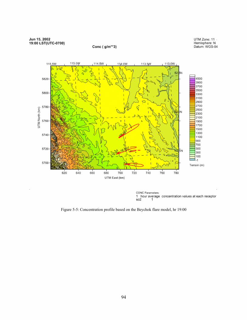
94
Figure 5-5: Concentration profile based on the Beychok flare model, hr 19:00

95
Figure 5-6: Concentration profile based on this study flare model, hr 19:00
Applying Surfer mapping software (Golden Software Inc., Golden, Colorado) for CALPOST
output files help us to compare these concentration profiles precisely.
Figures 5-7 to 5-11 compare the ground level concentrations of SO2 for each simulation in some
constant latitude and longitude for different sources.

96
Figure 5-7: Concentration of SO2 at hr 06:00 for X=699.56 km, near P1
0
5
10
15
20
25
30
35
40
45
50
5734 5736 5738 5740 5742 5744 5746 5748 5750
conc
entr
atio
n (1
0-7g/
m3 )
Y (km)
New Flare Model
Beychok Flare Model

97
Figure 5-8: Concentration of SO2 at hr 06:00 for Y=5739.66 km, near P1
0
5
10
15
20
25
30
35
40
45
692 694 696 698 700 702 704 706 708 710
conc
entr
atio
n (1
0-7g/
m3 )
X (km)
New FlareModel
BeychokFlareModel

98
Figure 5-9: Concentration of SO2 at hr 08:00 for X=691.46 km, near P2
0
2
4
6
8
10
12
14
16
5710 5712 5714 5716 5718 5720 5722
conc
entr
atio
n (1
0-7g/
m3 )
Y (km)
New FlareModel
BeychokFlareModel

99
Figure 5-10: Concentration of SO2 at hr 08:00 for Y=5715.36 km, near P2
0
2
4
6
8
10
12
14
684 686 688 690 692 694 696 698 700
conc
entr
atio
n (1
0-7g/
m3 )
X (km)
New FlareModel
BeychokFlareModel

100
Figure 5-11: Concentration of SO2 at hr 19:00 for Y=5697.36 km, near P3
As is shown in the above figures, the simulation based on the new flare model generally predicts
a higher concentration of the pollutant than the simulation based on the Beychok flare model for
the near field. In some cases, especially for moderate wind speed, both approaches have almost
the same results. This is due to height of the flare which is predicted to be similar in both flare
models. However, the results vary by a factor of two in the case of low or high wind speed.
On the other hand, for the far field the results are completely different. For areas far from
sources, it is the Beychok flare model which predicts higher concentration. Figures 5-12 and 5-
13 show the concentration of the pollutant far from any sources in some random coordinates.
0
1
2
3
4
5
6
7
8
9
700 705 710 715 720 725 730
conc
entr
atio
n (1
0-7g/
m3 )
X (km)
New FlareModel
BeychokFlareModel

101
Figure 5-12: Concentration of SO2 at hr 19:00 for Y=5754.06 km
0
0.2
0.4
0.6
0.8
1
1.2
1.4
718 720 722 724 726 728 730 732
conc
entr
atio
n (1
0-7g/
m3 )
X (km)
New FlareModel
BeychokFlareModel

102
Figure 5-13: Concentration of SO2 at hr 06:00 for X=714.86 km
Since the discussed flare model is sensitive to the wind speed, at low wind speed it predicts
greater flame heights than the Beychok model. In contrast, for high wind speed, the discussed
model predicts less flame height.
0
0.05
0.1
0.15
0.2
0.25
0.3
0.35
0.4
5718 5720 5722 5724 5726 5728 5730 5732
conc
entr
atio
n (1
0-7g/
m3 )
Y (km)
New FlareModel
BeychokFlareModel

6.1 Conc
In this st
simple (o
and form
equations
paramete
This rese
based on
of the fla
assumed
assumpti
separate
basic mo
lengths a
optimize
entrained
In the sec
sake of s
emissivit
emissivit
particulat
species. C
flaring of
flare para
model pr
contribut
model pr
clusion
tudy a simp
one-dimensio
med a set of
s. These aux
ers, and inclu
earch consis
n the previou
are assuming
that the
ons prevent
species in th
odel simple a
and angles a
d by adjusti
d air mixed i
cond section
simplicity, re
ty of the flar
ties of the ga
te matter, an
Comparing t
f pure metha
ameters such
redicts that th
tions of wat
redicts that a
Chapte
le and comp
onal) mome
f differential
xiliary equat
uding the rat
sts of three m
us work by D
g that 25%
combustion
ted the use
he flare, and
and fast to ru
ccurately. T
ing the entra
nto the burn
n, the basic m
eactions in th
re was calcu
aseous speci
nd the total e
the basic and
ane is close t
h as height a
he emissivity
ter and carb
about 10% o
Concer Six:
prehensive f
entum, mass,
equations w
tions are resp
te of reaction
main section
De Visscher
of heat prod
n reaction
of a compl
d the reactio
un, however
The fit betwe
ainment para
ning part of t
model was i
he combusti
ulated in a m
ies in the fla
emissivity w
d improved m
to instantane
and length pr
y of the flam
bon monoxid
of the produc
103
clusion and
flare model
, and energy
which need
ponsible for
n into the mo
ns. In the fir
(2009). The
duced by fla
occurs ins
lete formula
on rate of co
r the model
een the meas
ameters and
he flame and
mproved to
ion of pure m
more compreh
re were cons
was calculated
model illustr
eous. As a re
redicted are
me is predom
de are negli
ced heat is l
Future Wo
was develop
y balances. A
to be solve
r calculating
odel.
rst part, the
e basic mode
aring is emit
stantaneously
ation for ca
ombustion. T
is still able
surement da
the relation
d the flare ga
include the
methane wer
hensive met
sidered sepa
d according
rates that the
esult, the tem
almost the s
minantly due
igible. In ty
lost as radiat
ork
ped. This m
All equation
d along with
the emissiv
basic mode
el predicts th
tted by radia
y. These t
alculating th
These assum
to reproduc
ata and the m
nship betwee
as/wind velo
rate of the r
re considere
thod. In the
arately from
to the total o
e combustio
mperature pr
same in the b
to particulat
ypical flaring
tion, which
model is base
ns were comb
h some aux
vity, entrainm
el was devel
he character
ation. It was
two simpli
e emissiviti
mptions mak
e observed f
model values
en the fracti
ocity ratio.
reactions. Fo
ed. Moreove
improved m
the emissiv
optical dens
n reactions i
rofile and als
both models
te matter, an
g conditions
corresponds
ed on
bined
xiliary
ments
loped
ristics
s also
ifying
es of
ke the
flame
s was
on of
or the
er, the
model,
ity of
ity of
in the
so the
s. The
nd the
s, the
s with
104
the value used in the GPSA Handbook. It follows that the new emissivity calculation is a marked
improvement of the model, whereas the inclusion of reaction kinetics is a non-essential part of
the model, and was not retained in the next section of this work.
In the last part the effect of implementing the basic flare model in the CALPUFF air dispersion
model was investigated. A different flare model by Beychok (2005) was taken into account to
compare the results of its effects in the CALPUFF simulation with the proposed model.
Concentration profiles for each simulation show that the dispersion simulation based on the
proposed model tends to predict higher concentrations of contaminants in the near field while the
simulation based on the Beychok method shows the concentration of contaminants higher than
the proposed model for the far field of sources. These differences in some cases are more than
100 percent, which is considerable.
This simple structure of the new proposed flare model allows it to be embedded into the air
dispersion modeling software (such as CALPUFF) easily. Currently, regulatory models use
variants of Beychok’s (2005) approach which is not as accurate as the discussed model. More
sophisticated models exist (e.g. based on CFD), but these are too complex to be used in
combination with air dispersion models.
6.2 Future Work
In this study fmix, a variable that described the fraction of air mixed into the flame that takes part
in the combustion, is a function of ratio of the wind speed to the exit stack gas velocity. To
calculate its value, results of the basic model were calibrated to some observed data. Computing
values for fmix for different exit stacks and wind speeds could be improved by calibrating to more
experimental and observed data with a greater variety of wind speeds and exit stack velocities.
In this study of flames from flares it is assumed that flaring achieves complete combustion.
However, flaring is rarely successful in burning with 100% efficiency. EPA (2000) has reported
a value of 98% for flare combustion efficiency for properly operated flares, however flaring
gases with low heats of combustion has been shown to have efficiencies as low as 65%
(Blackwood, 2000). Since efficiency of the flare directly affects the calculation of the heat

105
generation and the flame length in the model, including the efficiency of flaring into the model
could improve the accuracy of the model. Although relatively accurate CFD models for the
efficiency of flaring have been provided by Blackwood (2000), Castineira and Edgar (2008), and
Singh et al. (2012), these models cannot be included in this flare model due to their complexity
and computation time. Instead, the empirical models of Johnson and Kostiuk (2002) or Leahey
and Preston (2001) for the efficiency of flaring can be applied for this purpose.
To validate the results in the CALPUFF air dispersion model, the flare model could be compared
to other flare models such as the flare model which is used by the Energy Resources
Conservation Board (ERCB). In addition, the resolution of the terrain in the CALPUFF
simulation also can be increased for a better understanding of local effects of flaring to the
dispersion of contaminants.
Finally, the main goal of this study is to improve the accuracy of dispersion modeling in air
dispersion model such as CALPUFF. Hence, the next step would be embedding this model into
the dispersion model code. This would enable the dispersion models to model the flare stacks
directly. For example, translating this model into the Fortran programing language and compiling
the code with CALPUFF dispersion codes, would prepare a flare module in the CALPUFF
model. Therefore, CALPUFF would be able to simulate air dispersion from the flare stacks more
accurately.

106
References
American Petroleum Institute (1969), “Guide for pressure relief and depressuring systems”, API RP 521,
First Edition
Argyropoulos, C.D., Sideris, G.M., Christolis, M.N., Nivolianitou, Z., Markatos N.C. (2009), “Modelling
pollutants dispersion and plume rise from large hydrocarbon tank fires in neutrally stratified atmosphere”,
Atmos. Environ., Vol. 44, pp. 803-813
Arya, S.P. (1999), “Air Pollution Meteorology and Dispersion”, Oxford University Press, New York
Benson, P.E. (1979), “CALINE3-A versatile dispersion model for predicting air pollutant levels near
highway and arterial streets”, Interim Report, Washington, D.C.
Beychok, M.R. (2005), “Fundamentals of Stack Gas Dispersion”, 4th edition, Beychok, Newport Beach,
CA
Bjorklund, J.R., Bowers, J.F. (1982), “User’s instructions for the SHORTZ and LONGZ computer
programs”, EPA-903/9-82-004a and b, U.S. Environmental Protection Agency, Philadelphia
Blackwood, R.B. (2000), “An evaluation of flare combustion efficiency using open-path Fourier
transform infrared technology”, J. Air Waste Manage. Assoc., Vol. 50, pp. 1714-1722
Bowers, J.R., Bjorklund, J.R., Cheney, C.S. (1979), “Industrial source complex (ISC) dispersion model
user’s guide”, EPA-450/4-79-030 and 031, U.S. Environmental Protection Agency, Research Triangle
Park, N.C.
Briggs, G.A. (1965), “A plume rise model compared with observations” J. Air Pollut. Control Assoc.,
Vol. 15, pp. 433
Briggs, G.A. (1968), “Concawe meeting: Discussion of the comparative consequences of different plume
rise formulas”, Atmos. Environ., Vol. 2, pp. 228-232
Briggs, G.A. (1969), "Plume Rise", AEC Critical Review Series, U.S. AEC Technical Information
Center, Oak Ridge, TN
107
Briggs, G.A. (1972), “Discussion: chimney plumes in neutral and stable surroundings”, Atmos. Environ.,
Vol. 6, pp. 507-510
Briggs, G.A. (1975), “Plume rise prediction”, Lectures on Air Pollution and Environmental Impact
Analyses, pp. 59-111, Am. Met. Soc., 34 Beacon Street, Boston, MA 02108, USA
Brzustowski, T.A. (1976), “Flaring in the energy industry”, Prog. Energy Combust. Sci., Vol. 2, pp. 129-
141
Burt, E.W. (1977), “VALLEY model user’s guide”, EPA-450/2-77-018, U.S. Environmental Protection
Agency, Research Triangle Park, N.C.
Castineira, D., Edgar, T.F. (2008), “CFD for simulation of crosswind on the efficiency of high
momentum jet turbulent combustion flames”, J. Environ. Eng., Vol. 7, pp. 561871
Catalano, J.A., Turner, D.B., Novak, J.H. (1987), “User’s guide for RAM”, 2nd Edition, EPA-600/3-87-
046, U.S. Environmental Protection Agency, Research Triangle Park, N.C.
Colbeck, I., Atkinson, B., Johar, Y. (1997), “The morphology and optical properties of soot produced by
different fuels”, J. Aerosol Sci., Vol. 28, pp. 715–723
Cooper, C.D., Alley, F.C. (2011), “Air Pollution Control”, Waveland Press Inc., Long Grove, Illinois
Cooper, C.D., Alley, F.C., Overcamp, T.J. (1982), “Hydrocarbon Vapor Incineration Kinetics”, Environ.
Prog., Vol. 1, pp. 129-133
De Visscher, A. (2009), “Extending the prime plume rise model to include flare combustion”,
Proceedings 8th World Congress of Chemical Engineering, Montreal, Canada
De Visscher, A. (2013), “Air Dispersion Modeling. Foundations and Applications”, J.Wiley & Sons,
forthcoming
DiCristofaro, D.C., Hanna, S.R. (1989), “OCD: The offshore and coastal dispersion model”, Version 4,
Vols. 1 and 2, Westford, MA
108
Dobbins, R.A., Mulholland, G.W., Bryner, N.P. (1994), “Comparison of a fractal smoke optics model
with light extinction measurements”, Atmos. Environ., Vol. 28, pp. 889–897
Dobbins, R.A., Megaridis, M. (1991), “Absorption and scattering of light by polydisperse aggregates”,
Appl. Optics, Vol. 30, pp. 4747–4754
Dryer, F.L., Glassman, I. (1973), “High-temperature oxidation of CO and CH4”, 14th Symposium
(International) on Combustion, Pittsburgh, PA: The Combust. Inst., pp. 987
Environment Canada website (2012), viewed September 01, 2012 <http://www.ec.gc.ca/ges-
ghg/default.asp?lang=En&n=DDCA72D0-1>
EPA (1988), “Screening producers for estimating the air quality impact of stationary sources, draft for
public comment”, EPA-450/4-88-010, U.S. Environmental Protection Agency, Research Triangle Park,
N.C.
EPA (1989), “User’s guide to the complex terrain dispersion model plus algorithms for unstable situation
(CTDMPLUS)”, Vol. 1, EPA-600/8-89-041, U.S. Environmental Protection Agency, Research Triangle
Park, N.C.
EPA (1990a), “User’s guide to the urban airshed model”, Vols. 1-8, EPA-454/B-93-004, U.S.
Environmental Protection Agency, Research Triangle Park, N.C.
EPA (1990b), “User’s guide to TSCREEN: A model for screening toxic air pollutant concentrations”,
EPA-450/4-91-013, U.S. Environmental Protection Agency, Research Triangle Park, N.C.
EPA (1992a), “The SCREEN2 model user’s guide”, EPA-450/4-92-006, U.S. Environmental Protection
Agency, Research Triangle Park, N.C.
EPA (1992b), “User’s guide for the industrial source complex (ISC2) dispersion model”, Vols. 1-3, EPA-
450/4-92-008a, b, and c, U.S. Environmental Protection Agency, Research Triangle Park, N.C.
EPA (1995), “User’s guide for the industrial source complex (ISC3) dispersion models”, Vols. 1-3, EPA-
454/B-95-003a, b, and c, U.S. Environmental Protection Agency, Research Triangle Park, N.C.

109
EPA (2003), “Appendix W to part 51-Guideline on Air Quality Models”, U.S. Environmental Protection
Agency, 68 FR 18448, Research Triangle Park, N.C.
Ezzati, M., Lopez, A.D., Vander Hoorn, S., Murray, C.J.L. (2002), “Selected major risk factor and global
and regional burden of disease”, Lancet, Vol. 360, pp. 1347-1360
Fairweather, M., Jones, W.P., Lindstedt, R.P., Marquis, A.J. (1991), “Prediction of a turbulent reacting jet
in a cross-flow”, Combust. Flame, Vol. 84, pp. 361-375
Forster, P., Ramaswamy, V., Artaxo, P., Berntsen, T., Betts, R., Fahey, D.W., Haywood, J., Lean, J.,
Lowe, D.C., Myhre, G., Nganga, J., Prinn, R., Raga, G., Schulz, M., Van Dorland, R. (2007), “Changes in
atmospheric constituents and in radiative forcing. In: climate change 2007: The physical science basis.
Contribution of working group I to the fourth assessment report of the intergovernmental panel on climate
change [Solomon, S., D. Qin, M. Manning, Z. Chen, M. Marquis, K.B. Averyt, M.Tignor and H.L. Miller
(eds.)]”, Cambridge University Press, Cambridge, United Kingdom and New York, NY, USA
Fraser, S. (2011), “Estimating intake fraction by loose-coupling an air dispersion model and a geospatial
information system (GIS)”, Master of Science Thesis, University of Calgary, Calgary, Alberta
GPSA (2012), GPSA Data Book, 13th Ed., Gas Processors Supplies Association
Hernandez, J., Crespo, A., Duijm, N.J. (1995), “Numerical modeling of turbulent jet diffusion flames in
the atmospheric surface layer”, Combust. Flame, Vol. 101, pp. 113-131
Hewitt, C. (2001), “The atmosphere chemistry of sulfur and nitrogen in power station plumes”, Atmos.
Environ., Vol. 35, pp. 1155-1170
Hottel, H.C., Egbert, R.B. (1942), Trans. Am. Inst. Chem. Eng., Vol. 38, pp. 531
Hoult, D.P., Weil, J.C. (1972), “Turbulent plume in laminar cross flow”, Atmos. Environ., Vol. 6, pp.
513-531
Howard, J.B., Williams, G.E., and Fine, D.H. (1973), “Kinetics of carbon monoxide oxidation in
postflame gases”, 14th Symposium (International) on Combustion, Pittsburgh, PA: Combust. Inst., pp. 975

110
Irwin, J.S., Chico, T., Catalano, J. (1985), “CDM 2.0 (climatological dispersion model) user’s guide”,
U.S. Environmental Protection Agency, Research Triangle Park, N.C.
Johnson, M. (2010) “Measuring PM emission in the upstream oil and gas industry”, presentation in
Petroleum Technology Alliance of Canada Air Issues Forum, Calgary, AB, Canada
Johnson, M.R., Devillers, R.W., Yang, C., Thomson, K.A. (2010) “Sky-scattered solar radiation based
plume transmissivity measurement to quality soot emissions from flares”, Environ. Sci. Technol., Vol. 44,
pp. 8196-8202
Johnson, M.R., Kostiuk, L.W. (2002), “A parametric model for the efficiency of a flare in crosswind”,
Proc. Combust. Inst., Vol. 29, pp. 1943-1950
Jones, H.R.N., (2000) “Radiation Heat Transfer”, Oxford University Press Inc., New York
Kalghatgi, G.T. (1983) “The visible shape and size of a turbulent hydrocarbon jet diffusion flame in a
cross wind”, Combust. Flame, Vol. 52, pp. 91-106
Lawal, M.S., Fairweather, M., Ingham, D.B., Ma, L., Pourkashanian, M., Williams, A. (2010),
“Numerical study of emission characteristics of a jet flame in cross-flow”, Combust. Sci. Technol., Vol.
182, pp. 1491-1510
Leahey, D.M., Paskall, H.G., Schroeder, M.B., Zelensky, M.J. (1985), “A preliminary study of the
chemical composition and combustion efficiency of a sour gas flare”, Alberta Environment, Research
Management Division Report 85/30, Edmonton, Alberta, Canada
Leahey, D.M., Preston, K. (2001), “Theoretical and observational assessments of flare efficiencies”, J. Air
Waste Manage. Assoc., Vol. 51, pp. 1610-1616
Leahey, D.M., Schroeder, M.B. (1987), “Observations and predictions of jet diffusion flame behavior”,
Atmos. Environ., Vol. 21, No. 4, pp. 777-784
Leahey, D.M., Schroeder, M.B. (1990), “Observations and predictions of jet diffusion flame behavior -
reply”, Atmos. Environ., Vol. 24a, pp. 2527-2529

111
Leckner, B. (1972), “Spectral and total emissivity of water vapor and carbon monoxide”, Combust.
Flame, Vol. 19, pp. 33-48
Liousse, C., Cashier, H., Jennings, S.G. (1993), “Optical and thermal measurements of black carbon
aerosol content in different environments: variation of specific attenuation cross section, sigma (σ)”,
Atmos. Environ., Vol. 27, pp. 1203-1211
Liu, D.H.F., Liptak, B.G. (2000), “Air Pollution”, Lewis Publishers, Boca Raton, FL
Lorimer, G. (1986), “The AUSPLUME Gaussian plume dispersion model”, Environmental Protection
Authority of Victoria, Melbourne, Victoria, Australia
Moosmuller, H., Arnott, W.P., Rogers, C.F., Chow, J.C., & Frazier, C.A. (1998), “Photoacoustic and
Filter measurements related to aerosol light absorption during the Northern Front Range Air Quality
Study (Colorado 1996/1997)”, J. Geophys. Res., Vol. 103, pp. 28149–28157
National Institute of Water and Atmospheric Research, Aurora Pacific Limited, and Earth Tech
Incorporated (2004), “Good practice guide for atmospheric dispersion modeling”, a report for Ministry
for the Environment, ISBN: 0-478-18941-9, Wellington, New Zealand
Nuclear Regulatory Commission (1972), “Safety Guide 123, onsite meteorological programs”, EPRI
Report EC-137
Paine, R.J. Strimaitis, D.G., Dennis, M.G., Yamartino, R.J., Mills, M.T., Insley, E.M. (1987), “User’s
guide to the complex terrain dispersion model”, Vol. 1, EPA-600/8-87-058a, U.S. Environmental
Protection Agency, Research Triangle Park, N.C.
Paine, R.J., Egan, B.A. (1987), “User’s guide to the rough terrain diffusion model (RTDM)”, Rev. 3.20
Perry, R.H, Green, D. (1984), “Perry’s Chemical Engineers’ Handbook”, McGraw-Hill, 5th Edition,
Singapore
Perry, S.G, Burns, D.J., Adams, L.H., Paine, R.J., Dennis, M.G., Mills, M.T., Strimaitis, D.G.,
Yamartino, R.J., Insley, E.M. (1989), “User’s guide to the complex terrain dispersion model plus
algorithm for unstable situation (CTDMPLUSS)”, Vol. 1, EPA-600/8-89-041, U.S. Environmental
Protection Agency, Research Triangle Park, N.C.

112
Perry, S.G., Burns, D.J., Adams, L.H., Paine, R.J., Dennis, M.G., Mills, M.T., Strimaitis, D.G.,
Yamarantino, R.J., Insley, E.M. (1989), “User’s guide to the complex terrain dispersion model plus
algorithm for unstable situation (CTDMPLUS) volume 1: model description and user instruction”, EPA-
600/8-89/041, U.S. Environmental Protection Agency, Research Triangle Park, NC
Perry, S.G., Burns, D.J., Cimorelli, A.J. (1990), “User’s guide to CDTMPLUS”, Vol. 2, EPA-600/8-90-
087, U.S. Environmental Protection Agency, Research Triangle Park, N.C.
Sandler, S.I. (1999), “Chemical, Biological and Engineering Thermodynamic”, 3rd Edition, USA, Wiley
Schnaiter, M., Horvath, H., Mohler, O., Naumann, K.H., Saathoff, H., Schock, O.W. (2003), “UV-VIS-
NIRspectral optical properties of soot and soot-containing aerosols”, J. Aerosol Sci., Vol. 34, pp. 1421-
1444
Schulman, L.L., Scire, J.S. (1980), “Buoyant line and point source (BLP) dispersion model user’s guide”,
Doc. P-7304B, Concord, Mass.
Schulman, L.L., Strimaitis, D.G., Scire, J.S. (2000), “Development and evaluation of the PRIME plume
rise and building downwash model”, J. Air Waste Manage. Assoc., Vol. 50, pp. 378–390
Scire, J.S., Lurman, F.W., Bass, A., Hanna, S.R (1984b), “User’s guide to the MESOPUFF II model and
related processor programs”, EPA-600/8-84-013, U.S. Environmental Protection Agency, Research
Triangle Park, N.C.
Scire, J.S., Lurman, F.W., Bass, A., Hanna, S.R. (1984a), “Development of the MESOPUFF II dispersion
model”, EPA-600/3-84-057, U.S. Environmental Protection Agency, Research Triangle Park, N.C.
Scire, J.S., Strimaitis, D.G., Yamartino, R.J. (1990a), “Model formulation and user’s guide for the
CALMET meteorological model”, Prepared for California Air Resource Board by Sigma Research
Corporation, Concord, MA
Scire, J.S., Strimaitis, D.G., Yamartino, R.J. (1990b), “Model formulation and user’s guide for the
CALPUFF dispersion model”, Prepared for California Air Resource Board by Sigma Research
Corporation, Concord, MA

113
Scire, J.S., Strimaitis, D.G., Yamartino, R.J. (2000), “A user’s guide for the CALPUFF dispersion Model
(Version 5)”, Earth Tech, Inc.
Segal, H.M. (1988), “A microcomputer pollution model for civilian airports and air force basis - Model
application and background”, FAA-EE-88-5, Washington, D.C.
Segal, H.M. (1991), “EDMA - Microcomputer pollution model for civilian airports and air force basis:
User’s guide”, FAA-EE-91-3, Washington, D.C.
Segal, H.M., Hamilton, P.L. (1988), “A Microcomputer pollution model for civilian airports and air force
basis - Model description”, FAA-EE-88-4, Washington, D.C.
Seigel, R., Howel, J.R. (2002), “Thermal Radiation Heat Transfer”, 4th edition, Taylor & Francis, New
York
Singh, K.D., Dabade, T., Vaid, H., Gangadharan, P., Chen, D., Lou, H.H., Li, X., Li, K., Martin, C.B.
(2012), “Computational fluid dynamics modeling of industrial flares operated in stand-by mode”, Ind.
Eng. Chem. Res., Vol. 51, pp. 12611-12620
Smith, P.T., Thurston, C.M., Chambers, A. (2009), “Large eddy simulation of industrial flares”, viewed November 1, 2012, <http://www.flaresimulation.org/arc/>
Turner, B.C., Schulze, R.H. (2007), “Practical Guide to Atmospheric Dispersion Modeling”, Trinity
Consultants, Inc. and Air & Waste Management Association, Dallas, TX
Turner, D.B. (1994), “Workbook of Atmospheric Dispersion Estimates: An Introduction to Dispersion
Modeling”, 2nd Edition, Lewis Publishers
Turner, D.B., Novak, J.H. (1978), “User’s guide for RAM”, Vols. 1 and 2, Report EPA-600/8-78-016a
and b, U.S. Environmental Protection Agency, Research Triangle Park, N.C.
Wendt, J.F. (1992), “Computational Fluid Dynamics – An Introduction”, Springer-Verlag Berlin and
Heidelberg GmbH & Co. K, Berlin
Williams, G.C., Hottel, H.C., Morgan, A.C. (1969), “The combustion of methane in a jet-mixed reactor”,
12th Symposium (International) on Combustion, Pittsburgh, PA: The Combustion Institute, pp. 913

114
World Health Organization (2012), “Estimated deaths & DALYs attributable to selected environmental
risk factors, by WHO Member State, 2002”, viewed July 1, 2012.
<http://www.who.int/entity/quantifying_ehimpacts/countryprofilesebd.xls>

115
Appendices
Appendix A
Adiabatic Lapse Rate
This derivation is the calculation of the altitude dependence of temperature of what is called a
neutral atmosphere, or adiabatic atmosphere.
Start from the energy conservation law:
dU dq dW ................................................................................................................. equation 1
U is the internal energy (J) of the air parcel, q is the heat added to the air parcel (J), and W is the
work added to the air parcel (J). For adiabatic conditions it can be assumed that dq 0.
dU dW ........................................................................................................................... equation 2
On the other hand
U H pV ....................................................................................................................... equation 3
Differentiation leads to:
dU d H pV dH pdV Vdp ............................................................................. equation 4
The enthalpy change with temperature at constant pressure is the definition of the heat capacity
at constant pressure:
dH mc , dT ................................................................................................................ equation 5
Where m is the mass of the air parcel (kg), c , is the specific heat of air (J/kg K), and T is the
absolute temperature (K). Mechanical work is due to compression/expansion, and is given by:
dW pdV ..................................................................................................................... equation 6
The minus sign indicates that the work exerted on the air parcel is positive in compression.
Substitution of the energy conservation law equation with the above equation leads to:
dU pdV ...................................................................................................................... equation 7

116
Substitution of equations 5 and 7 into equation 4 leads to:
pdV mc , dT pdV Vdp
or
mc , dT Vdp .............................................................................................................. equation 8
The hydrostatic equation defines the altitude dependence of barometric pressure. This equation,
which is a force balance for a thin layer of area 1 m2, is given by:
Where p is barometric pressure (Pa), ρ is the density of the air (kg/m3), g is acceleration of
gravity (9.80665 m/s2), and z is the altitude (m). Canceling out p and rewriting leads to the
following equation:
Substituting the hydrostatic equation into equation 8 leads to:
mc , dT Vρgdz ....................................................................................................... equation 9
Since . :
c , dT gdz
Or
T
, ................................................................................................................. equation 10
The term ,
which is called the adiabatic Lapse Rate, is applied only for dry air. In the
presence of clouds or fog, the adiabatic Lapse Rate is given by:
T
, ∆ .................................................................................................... equation 11
Where is the water to air mass ratio

117
Appendix B
Coefficients to be used in Equation 4.45 for water vapor and carbon dioxide (Leckner, 1972)
Deviation from values calculated with spectral data is max ±5%.
Water vapor, T� 400, M=2, N=2
i c0i c1i c2i
0 -2.2118 -1.1987 0.035596
1 0.85667 0.93048 -0.14391
2 -0.10838 -0.17156 0.045915
Carbon dioxide, Hottels’s diagram, M=2, N=3
i c0i c1i c2i c3i
0 -3.3390 1.1996 -1.0604 0.16454
1 0.90786 0.086726 0.13797 -0.035144
2 -0.15563 -0.10292 0.064443 -0.014128

118
Appendix C
The basic flare model code
Data File:
tend = 20; step = 0.01; tspan = 0:step:tend; Uatm = 2; %wind speed (m/s) Tatm = 288; %T of atmosphere at height 0 (K) Patm = 101325; %atmosphere pressure (pa) lapse = -0.00975; %temperature lapse in the atmosphere
dTatm/dz) MO2 = 0.232; %mass fraction of oxygen in air Mgas = 0.016; %molar mass of gas in kg/mol Mair = 0.029; %molar mass of air in kg/km ROatm = Mair*Patm/8.314472/Tatm; %density of atmosphere (kg/m3) ROflame = Mgas*Patm/8.314472/Tatm; %density of flame (kg/m3) correction = 1.6; %correction for entertainment parameters
alpha and beta epsf = 0.0116; %emissivity of the flame epsair = epsf; %emissivity of the air thf = -log(1-epsf); %Flame Optical thickness thair = -log(1-epsair); %Air optical thickness th = thf + thair; %Overall Optical thickness sig = 5.67e-8; %Stefan-Boltzmann constant alpha = correction* 0.11; beta = correction*0.6;

119
n = 4; g = 9.81; dUatmdz=0; dstack = 0.10695; %diameter of stack(m) rstack = dstack/2; %radius of stack(m) hstack = 20; %height of stack(m) Qc = 10000; %heating value in kJ/s H = 50000; %heat of combustion in kJ/kg m = Qc/H; %mass flow rate (kg/s) Vrate = m/ROflame; %volumetric flow rate (m3/s) Area = pi*rstack*rstack; Ustk = Vrate/Area; %stack exit velocity p1 = Uatm/Ustk; Usc = Vrate/Area; %velocity of plume fmix = 0.0362*exp(4.5679*p1); %fraction of air mixing into the plume Tair = 288; %T of non-burning fraction of the flame Tf = 288; %T of burning fraction of the plume cpf = 1000; %specific heat of burning fraction of the
plume air (J/kg K) cpair = 1000; %specific heat of non-burning fraction of
the flame air (J/kg K) y0(1) = ROflame*Usc*rstack*rstack; y0(2) = 0; y0(3) = hstack; y0(4) = y0(1)*(0-Uatm); y0(5) = y0(1)*Usc; y0(6) = 0;

120
y1init = y0(1); y0(7) = y0(1); y0(8) = 0; y0(9) = 0; y0(10) = 0;

121
Function file:
function dydt = f (t,y,Uatm,Tatm,Patm,lapse,epsf,epsair,eps,thf,thair,th,sig,alpha,beta,n,g,dUatmdz,MO2,H,fmix,y1init,Mgas) x = y(2); z = y(3); u = Uatm + y(4)/y(1); w = y(5)/y(1); frac = y(7)/y(1); Tf = Tatm+y(8)/y(1)/frac; if frac == 1 Tair = Tf; else Tair = Tatm+y(9)/y(1)/(1-frac); end Tatm = Tatm+z*lapse; ROatm = 0.029*Patm/8.314472/Tatm; ROair = 0.029*Patm/8.314472/Tair; MWf = (Mgas*y1init + 0.029*(y(7) - y1init))/y(7); ROf = MWf*Patm/8.314472/Tf; RO = 1/(frac/ROf+(1-frac)/ROair); Usc = sqrt(u*u+w*w); cpf = 1.9327e-10*Tf^4-7.9999e-7*Tf^3+1.1407e-3*Tf^2-4.4890e-1*Tf+1.0575e+3; cpair = 1.9327e-10*Tair^4 - 7.9999e-7*Tair^3 + 1.1407e-3*Tair^2 - 4.4890e-1*Tair + 1.0575e+3; r = sqrt(y(1)/(RO*Usc)); dydt = zeros(10,1); dydt(1) = 2*r*alpha*ROatm*abs(Usc-Uatm*u/Usc)+2*r*beta*ROatm*abs(Uatm*w/Usc); dydt(2) = u/Usc;

122
dydt(3) = w/Usc; dydt(4)=-r*r*RO*w*dUatmdz; dydt(5)=g*r*r*(ROatm-RO); dydt(7) = fmix*dydt(1); dydt(6) = MO2/n/y1init*dydt(7); if y(6) > 1 dydt(6) = 0; end dydt(8) = y1init*(H*1000/cpf)*dydt(6)-frac*(lapse+g/cpf)*RO*w*r*r-(2*eps*sig*r*frac/cpf)*(Tf^4-Tatm^4); dydt(9) = -(1-frac)*(lapse+g/cpair)*RO*w*r*r; dydt(10) = (2*sig*(1-exp(-th))*r*(Tf^4-Tatm^4))/(cpf*y1init*H*(1000/cpf));

123
Main File:
data options = odeset('RelTol', 1e-6, 'AbsTol', 1e-8, 'InitialStep', 0.01); [T,Y] = ode45(@f,tspan,y0,options,Uatm,Tatm,Patm,lapse,epsf,epsair,eps,thf,thair,th,sig,alpha,beta,n,g,dUatmdz,MO2,H,fmix,y1init,Mgas); figure(1) plot(T,Y(:,6),'k','linewidth',2) title('X vs S') xlabel('S (distance aong the plume centerline, m)') ylabel('X-CH4 (conversion of combustion to CH4)') [s1,s2] = size(T); for i=1:s1 frac(i) = Y(i,7)/Y(i,1); Ta = Tatm + lapse*Y(i,3); Tf(i) = Ta + Y(i,8)/Y(i,1)/frac(i); end hold on figure(2) plot(T,Tf,'k','linewidth',2) title('Tf vs S') xlabel('S (distance along the plume centerline, m)') ylabel('Tf (temperature of the flare, T)') jj=0; uu=0; for i=1:100*tend+1 if Y(i,6)>0.999 & jj==0 jj=i; uu(jj)=T(i); end end flamelenght = uu(jj); flameheight = Y(jj,3)-20;

124
Appendix D
The improved flare model code
Data file:
tend = 10; step = 0.01; tspan = 0:step:tend; Uatm = 2; %wind speed (m/s) Tatm = 288; %T of atmosphere at height 0 (K) Patm = 101325; %atmosphere pressure (pa) lapse = -0.00975; %temperature lapse in the atmosphere
(dTatm/dz) MO2 = 0.232; %mass fraction of oxygen in air Mgas = 0.016; %molar mass of gas in kg/mol Mair = 0.029; %molar mass of air in kg/km ROatm = Mair*Patm/8.314472/Tatm; %density of atmosphere (kg/m3) ROflame = Mgas*Patm/8.314472/Tatm; %density of flame (kg/m3) correction = 1.6; %correction for entertainment parameters
alpha and beta epsf = 0.0085; %emissivity of the flame epsair = 0.0085; %emissivity of the air thf = -log(1-epsf); %Flame Optical thickness thair = -log(1-epsair); %Air optical thickness th = thf + thair; %Overall Optical thickness sig = 5.67e-8; %Stefan-Boltzmann constant alpha = correction*0.11; beta = correction*0.6;

125
n = 4; g = 9.81; dUatmdz=0; dstack = 0.10695; %diameter of stack(m) rstack = dstack/2; %radius of stack(m) hstack = 20; %height of stack(m) Qc = 10000; %heating value in kJ/s H1 = 32500; %heat of combustion in kJ/kg CH4 (to CO) H2 = 17500; % heat of combustion in kJ/kg CH4 (CO to
CO2) m = Qc/(H1+H2); %mass flow rate (kg/s) Vrate = m/ROflame; %volumetric flow rate (m3/s) Area = pi*rstack*rstack; Ustk = Vrate/Area; %stack exit velocity p1 = Uatm/Ustk Usc = Vrate/Area; %velocity of plume fmix = 0.0362*exp(4.5679*p1); %fraction of air mixing into the plume Tair = 288; %T of non-burning fraction of the flame Tf = 288; %T of burning fraction of the plume cpf = 1000; %specific heat of burning fraction of the
plume air (J/kg K) cpair = 1000; %specific heat of non-burning fraction of
the flame air (J/kg K) y0(1) = ROflame*Usc*rstack*rstack; y1init = y0(1); y0(2) = 0; y0(3) = hstack; y0(4) = y0(1)*(0-Uatm);

126
y0(5) = y0(1)*Usc; y0(6) = 0; y0(7) = y0(1); y0(8) = 0; y0(9) = 0; y0(10) = 0; y0(11) = 0;

127
Function file:
function dydt = f3(t,y,Uatm,Tatm,Patm,lapse,epsf,epsair,eps,thf,thair,th,sig,alpha,beta,n,g,dUatmdz,MO2,H1,H2,fmix,y1init,Mgas) dydt = zeros(11,1); x = y(2); z = y(3); u = Uatm + y(4)/y(1); w = y(5)/y(1); frac = y(7)/y(1); Tf = Tatm+y(8)/y(1)/frac; if frac == 1 Tair = Tf; else Tair = Tatm+y(9)/y(1)/(1-frac); end Tatm = Tatm+z*lapse; ROatm = 0.029*Patm/8.314472/Tatm; ROair = 0.029*Patm/8.314472/Tair; MWf = (Mgas*y1init + 0.029*(y(7) - y1init))/y(7); ROf = MWf*Patm/8.314472/Tf; RO = 1/(frac/ROf+(1-frac)/ROair); ROinit = Mgas*Patm/8.314472/Tatm; %density of burning gas in the initial point pf stack Usc = sqrt(u*u+w*w); cpf = 1.9327e-10*Tf^4-7.9999e-7*Tf^3+1.1407e-3*Tf^2-4.4890e-1*Tf+1.0575e+3; cpair = 1.9327e-10*Tair^4 - 7.9999e-7*Tair^3 + 1.1407e-3*Tair^2 - 4.4890e-1*Tair + 1.0575e+3; r = sqrt(y(1)/(RO*Usc));

128
%KINETIC CALCULATION if (y(6) < 1) yCH4 = y1init*(1-y(6)); else yCH4 = 0; end if (y(6) - y(11) > 0) yCO = y1init*(y(6) - y(11))*1.75; % mass flow rate of CO else yCO = 0; end yCO2 = y1init*y(11)*2.75; % mass flow rate of CO2 yH2O = y(6)*y1init*2.25; yO2 = (frac*y(1)-y1init)*MO2 - y1init*(3*y(6) + y(11)); yN2 = (frac*y(1)-y1init)*(1-MO2); ymCH4 = yCH4/0.016; ymCO2 = yCO2/0.044; ymH2O = yH2O/0.078; ymO2 = yO2/0.032; ymN2 = yN2/0.028; ymCO = yCO/0.028; ymsum = ymCH4 + ymCO2 + ymH2O + ymO2 + ymN2 + ymCO; ymfO2 = ymO2/ymsum; ymfCH4 = ymCH4/ymsum; ymfCO = ymCO/ymsum; ymfH2O = ymH2O/ymsum; Z = 1.011e11; %collision factor S = 1; %steric factor: S=16/MW R = 8.314; %gas constant (j/mol.k) RR = 0.08206; %gas constant (L.atm/mol.k)

129
E = (-0.00966*Mgas+46.1)*4.184*1000; %activation energy (j) A = (Z*S*ymfO2*Patm)/(RR); CCH4 = ymfCH4*Patm/R/Tf; CCO = ymfCO*Patm/R/Tf; CH2O = ymfH2O*Patm/R/Tf; dydt(1) = 2*r*alpha*ROatm*abs(Usc-Uatm*u/Usc)+2*r*beta*ROatm*abs(Uatm*w/Usc); dydt(7) = fmix*dydt(1); if t<1 && Tf<1000; k1 = Z*S*R*Tf/RR*exp(-E/8.314/1000); k2 = 1.3e8*exp(-30000*4.184/R/1000)*sqrt(CH2O); C_O2sqrt = (-0.032*0.5*k2*CCO+sqrt((0.032*0.5*k2*CCO)^2 + 4*0.032*1.5*k1*CCH4*dydt(7)*MO2/r/r))/(2*0.032*1.5*k1*CCH4); C_O2 = C_O2sqrt^2; rCH4 = k1*C_O2*CCH4; rCO2 = k2*CCO*C_O2sqrt; else k1 = Z*S*R*Tf/RR*exp(-E/8.314/Tf); k2 = 1.3e8*exp(-30000*4.184/R/Tf)*sqrt(CH2O); if CCH4 == 0 C_O2sqrt = (dydt(7)*MO2/r/r)/(0.032*0.5*k2*CCO); else C_O2sqrt = (-0.032*0.5*k2*CCO+sqrt((0.032*0.5*k2*CCO)^2 + 4*0.032*1.5*k1*CCH4*dydt(7)*MO2/r/r))/(2*0.032*1.5*k1*CCH4); end C_O2 = C_O2sqrt^2; rCH4 = k1*C_O2*CCH4; rCO2 = k2*CCO*C_O2sqrt; end %EMISSIVITY CALCULATION %SOOT EMISSIVITY CALCULATION c = 3e8; %speed of light (meter/sec) h = 6.626e-34; %Planck constant (J*sec) k = 1.38e-23; %Boltzman constant (J/K) landa = (c*h)/(4.96*k*Tf); cprime = 4000; %constant in: sigmaA=cprime/landa sigmaA = cprime/(landa*1e9); EF = 0.2; %emission factor (kg soot/1000m3 fuel)

130
cnst = (y1init*RO*EF*y(6))/(y(1)*ROinit*1000)*1000;
%concentration of soot (g soot/m3 plume) ODsoot = cnst*2*r*sigmaA; epssoot = 1 - exp(-ODsoot) %PARTIAL PRESSURE CALCULATION molCO2 = y1init*frac*0.044/0.016/0.044; %number of CO2 moles molH2O = y1init*frac*0.036/0.016/0.018; %number of H2O moles molT = y(1)*frac/MWf; %total number of moles in the flame pCO2 = (Patm/100000)*(molCO2/molT); %partial pressure of CO2(bar) pH2O = (Patm/100000)*(molH2O/molT); %partial pressure of HO2 (bar) %H2O EMISSIVITY CALCULATION if Tf>750 taw = Tf/1000; else taw = 0.75; end taw = abs(taw); if taw>2.4 taw = 2.4; end landaP = log10(abs(pH2O/100000*2*r*100*frac));
%constant used in other equations A = 1.888 - 2.053*log10(taw); %constant used in other equations B = 1.10*taw^(-1.4); %constant used in other equations a0 = -2.2118 - 1.1987*taw + 0.035596*taw^2;
%a0-a2 constant used in other equations a1 = 0.85667 + 0.93048*taw - 0.14391*taw^2; a2 = -0.10838 - 0.17156*taw + 0.045915*taw^2; eps0H2O = exp(a0 + a1*landaP + a2*landaP^2); %emissivity at pressure of 1 bar PEH2O = Patm/100000*(1 + 4.9*pH2O/(Patm/100000)*sqrt(273/Tf)); %equivalent pressure of H2O

131
epH2O = (A*PEH2O + B)/(PEH2O + A + B -1); %portion of actual emissivity to emissivity at pressure of 1 bar
epsH2O = epH2O*eps0H2O; %actual emmisivity of H2O %CO2 EMISSIVITY CALCULATION if Tf>750 taw = Tf/1000; else taw = 0.75; end taw = abs(taw); if taw>2.4 taw = 2.4; end landaP = log10(abs(pCO2/100000*2*r*100*frac)); %constant used in other equations A = 0.1*taw^(-1.45) + 1;
%constant used in other equations B = 0.23; %constant used in other equations a0 = -3.3390 + 1.1996*taw - 1.0604*taw^2 + 0.16454*taw^3; %a0-a3 constant used in other equations a1 = 0.90786 + 0.086726*taw + 0.13797*taw^2 - 0.035144*taw^3; a2 = -0.15563 - 0.10292*taw + 0.064443*taw^2 - 0.0141128*taw^3; eps0CO2 = exp(a0 + a1*landaP + a2*landaP^2);
%emissivity at pressure of 1 bar PECO2 = Patm/100000*(1 + 4.9*pCO2/(Patm/100000)*sqrt(273/Tf));
%equivalent pressure of H2O epCO2 = (A*PECO2 + B)/(PECO2 + A + B -1);
%portion of actual emissivity to emissivity at pressure of 1 bar
epsCO2 = epCO2*eps0CO2; %actual emissivity of CO2 %TOTAL EMISSIVITY OF CO2/H2O/SOOT x = pH2O/(pH2O + pCO2); %constant used in other equation landaP = log10(abs((pCO2+pH2O)/100000*2*r*100*frac)); %constant used in other equations if landaP < 0

132
landaP = 0; end deltae = (x/(10.7 + 101*x) - 0.0089*x^10.4)*landaP^2.76;
%overlap correction epsCO2H2O = epsH2O + epsCO2 - deltae; ODCO2H2O = -log(1-epsCO2H2O); % Optical density of carbon monoxide ODtotal = ODsoot + ODCO2H2O; %Total optical density eps = 1-exp(-ODtotal); %total emissivity %DIFFERENTIAL EQUATIONS dydt(1) = 2*r*alpha*ROatm*abs(Usc-Uatm*u/Usc)+2*r*beta*ROatm*abs(Uatm*w/Usc); dydt(2) = u/Usc; dydt(3) = w/Usc; dydt(4)=-r*r*RO*w*dUatmdz; dydt(5)=g*r*r*(ROatm-RO); if y(6) > 1 dydt(6) = 0; else dydt(6) = Mgas*r*r*rCH4/y1init; end dydt(7) = fmix*dydt(1); if y(11) > 1 dydt(11) = 0; else dydt(11) = Mgas*r*r*rCO2/y1init; end dydt(8) = y1init*(H1*1000/cpf)*dydt(6)+y1init*(H2*1000/cpf)*dydt(11)-frac*(lapse+g/cpf)*RO*w*r*r-(2*eps*sig*r*frac/cpf)*(Tf^4-Tatm^4); dydt(9) = -(1-frac)*(lapse+g/cpair)*RO*w*r*r; dydt(10) = (2*sig*(1-exp(-th))*r*(Tf^4-Tatm^4))/(cpf*y1init*(H1+H2)*(1000/cpf));

133
Main file:
data options = odeset('RelTol', 1e-6, 'AbsTol', 1e-8, 'InitialStep', 0.01); [T,Y] = ode45(@f3,tspan,y0,options,Uatm,Tatm,Patm,lapse,epsf,epsair,eps,thf,thair,th,sig,alpha,beta,n,g,dUatmdz,MO2,H1,H2,fmix,y1init,Mgas); figure(1) plot(T,Y(:,6),':b','linewidth',2) title('X vs S') xlabel('S (distance along the plume centerline, m)') ylabel('X-CH4 (conversion of combustion to CH4)') hold on figure(3) plot(T,Y(:,11),'--r','linewidth',2) title('X-CO2 vs S') xlabel('S (distance along the plume centerline, m)') ylabel('X-CO2 (conversion of combustion to CO2)') [s1,s2] = size(T); for i=1:s1 frac = Y(i,7)/Y(i,1); Ta = Tatm + lapse*Y(i,3); Tf(i) = Ta + Y(i,8)/Y(i,1)/frac; end hold on figure(2) plot(T,Tf,'-.m','linewidth',2) title('Tf vs S') xlabel('S (distance aong the plume centerline, m)') ylabel('Tf (temperature of the flare, T)')

134
jj=0; uu=0; for i=1:100*tend+1 if Y(i,11)>0.999 && jj==0 jj=i; uu(jj)=T(i); end end flamelenght = uu(jj); flameheight = Y(jj,3)-20;