Available online at www.sciencedirect.com

www.elsevier.com/locate/asr

Advances in Space Research 48 (2011) 826–836

The geomagnetic solar flare effect identified by SIIG as an indicatorof a solar flare observed by GOES satellites

M.A. Van Zele a,b, A. Meza b,c,⇑

a Facultad de Ciencias Exactas y Naturales, Universidad de Buenos Aires, Argentinab Consejo Nacional de Investigaciones Cientıficas y Tecnicas (CONICET), Buenos Aires, Argentina

c Facultad de Cs. Astronomicas y Geofısicas, Universidad Nacional de La Plata, La Plata, Argentina

Received 9 February 2011; received in revised form 27 April 2011; accepted 28 April 2011Available online 7 May 2011

Abstract

This paper studies the efficiency of geomagnetic solar flare effects (gsfe) in X solar flare detection; so during the period 1999–2007 acomparison between solar flare (sf) observed by satellites of the Geostationary Operational Environmental Satellite (GOES) programmeand gsfe published by the Service International des Indices Geomagnetiques (SIIG) is made.

Solar flares (sfs) are one of the most powerful manifestations of the solar activity. Because the far UV and soft and hard X-ray solarflare radiation is absorbed by the ionosphere, the ionized gas density increases (ionospheric solar flare effect, isfe) and a sudden enhance-ment of geomagnetic field near Earth surface (geomagnetic solar flare effect, gsfe) is produced.

The solar X-ray flux is systematically recorded since 1975 by GOES satellites, and gsfe are declared by geomagnetic observatoriessince 1957. We corroborate that the identification of sf using gsfe is affected by several factors:

– the intensity and average growth rate of solar flare radiation when quicker is it more easily the sf is detected as gsfe;

– the position of the geomagnetic observatory, we found that observatories placed at summer hemisphere identify more easily the sf, sothe uneven geographical distribution of observatories make the sf identification difficult;

– the existing geomagnetic perturbation previous to sf, and the likeness between the gsfe and other geomagnetic variations.

This work shows that gsfe recorded as associated to sf is a poor detector of sf even if it is intense. Some of these inconveniences can beavoided if the distribution of the observatories is improved and the identification of a sf is made using simultaneously gsfe, solar windparameters and isfe.� 2011 COSPAR. Published by Elsevier Ltd. All rights reserved.

Keywords: Solar flare; Geomagnetic field; GPS; Vertical total electron content

1. Introduction

Sun and other cosmic sources have a strong influence oninterplanetary space, the Earth’s magnetosphere, iono-sphere, and thermosphere; so the space weather is a highlyrelevant subject of research and many authors have made

0273-1177/$36.00 � 2011 COSPAR. Published by Elsevier Ltd. All rights rese

doi:10.1016/j.asr.2011.04.037

⇑ Corresponding author at: Consejo Nacional de InvestigacionesCientıficas y Tecnicas (CONICET), Buenos Aires, Argentina. Tel.: +54221 4236593; fax: +54 221 4236591.

E-mail address: ameza@fcaglp.unlp.edu.ar (A. Meza).

contributions on these topics (Baker, 2000; Siscoe, 2000;Echer et al., 2005).

The sun is the most powerful source of energy in oursolar system. It primarily emits energy in the form of elec-tromagnetic radiation and the magnetic structure of theSun’s photosphere varies continuously transient processessuch as micro flares, shock waves, erupting prominences,flares and coronal mass ejections. These processes causeshort time increases of EUV-, X-ray, gamma-ray andradio-wave emissions. In addition to the radiation, the

rved.

Table 1List of geomagnetic observatories, their coordinates, and time (UT) atnoon.

Observatory IAGA code Lat.(�)

Long.(�)

Time (UT) atnoon

Canberra CNB 35S 149E 2.1Memambetsu MMB 44N 144E 2.4Kakioka KAK 36N 140E 2.7Hatizyo HTY 33N 140E 2.7Kanoya KNY 31N 131E 3.3Lunping LNP 25N 121E 3.9Gnangara GNA 32S 116E 4.3Hyderabad HYB 17N 79E 6.7Ettaiyapuram ETT 9N 78E 6.8Quetta QUE 30N 67E 7.5Hermanus HER 34S 19E 10.7Hurbanovo HRB 48N 18E 10.8Nagycenk NCK(NAG) 48N 17E 10.9Budkov BDV 49N 14E 11.1Niemegk NGK 52N 13E 11.2Wingst WNG 54N 9E 11.4Chambon la

ForetCLF 48N 2E 11.9

Ebro EBR 41N 0E 12Lerwick LER 60N 1W 12.1Eskdalemuir ESK 55N 3W 12.2Hartland HAD 51N 3W 12.2S.Pablo-Toledo SPT 40N 4W 12.3Valentia VAL 52N 10W 12.7Guimar GUI 28N 16W 13.1

Table 2Number of sf recorded by GOES satellites according to X-ray classification, a

Year sf

X M C B A

1999 4 170 1855 389 02000 17 215 2233 166 02001 21 310 2102 273 02002 12 219 2320 164 02003 20 160 1332 917 02004 11 122 912 1324 22005 18 103 610 1449 02006 4 10 149 1031 22007 0 10 73 566 0

Table 3number of gsfe associated to a solar flare in X-rays/total number of sf in X-radeclared that are associated to sf.

Year Jan Feb Mar Apr May Jun

1999 1/1 0/3 3/5 2/3 7/9 7/12000 0/2 0/1 5/9 7/9 0/3 6/72001 4/8 1/3 4/4 9/10 1/3 102002 0/2 1/1 3/9 4/4 2/3 1/32003 1/2 0/1 1/3 3/8 1/3 3/62004 0/0 2/5 3/7 0/5 3/6 0/32005 2/4 0/0 0/1 0/0 3/6 2/22006 0/2 0/1 0/4 3/6 0/2 0/12007 0/2 0/0 0/3 0/4 0/1 5/5% 35 27 42 57 47 67

M.A. Van Zele, A. Meza / Advances in Space Research 48 (2011) 826–836 827

Sun also emits a stream of matter, which is called solarwind. The supersonic solar wind interacts with the terres-trial magnetic field by forming a standing bow shock thatslows, deflects and heats the plasma, so the solar wind con-trols the size of the magnetosphere and the energy flow intothe magnetosphere. The processes in magnetosphere causetwo major phenomena in the upper atmosphere: particleprecipitation and convection of the ionospheric plasma.When a quick flux of solar wind with a southward inter-planetary magnetic field reaches the magnetosphere theequatorial ring current is energized, producing the mainphase of a geomagnetic storm recorded as the decrease ofthe northern component of the geomagnetic field. Manyauthor have worked on ionospheric effects of flares andstorms (Tsurutani et al., 2005, 2008; Mannucci et al., 2008).

A solar flare (sf) is an intense and short-lived suddenrelease of energy produced by the increasing in the intensityof the emitted radiation. The different spectral ranges of theemitted radiation show a typical scheme. There is a “pref-lare” brightening generally lasting a few minutes, followedby the “impulsive” phase, which typically lasts a few min-utes and consists of bursts in gamma rays hard X-rays,EUV, and microwave radiation. After the impulsive phase,thermal radiation dominates; this is the gradual or decay-ing phase of the flare that can take several hours. It is seenas bright area on the Sun in optical wavelengths and asbursts of noise in radio wavelengths. The flare was tradi-tionally monitored in the Ha wavelength; currently the

nd the number of gsfe declared by the SIIG, associated to the sf or not.

gsfe

X M C B A Without association

3 32 9 0 0 27 (37%)5 19 12 0 0 23 (39%)8 37 9 0 0 21 (28%)8 21 1 0 0 22 (42%)4 14 4 0 0 38 (63%)6 17 5 0 0 27 (48%)9 14 0 2 0 15 (37%)3 2 1 1 0 27 (87%)0 4 1 0 0 18 (78%)

ys declared, separated by month for each year and the percentage of gsfe

Jul Aug Sep Oct Nov Dec

1 3/3 10/11 1/5 3/5 6/12 1/38/10 0/1 5/9 0/1 3=4 2/3

/13 0/2 3/6 12/13 3/5 2/3 4/69/13 4/4 3/5 1/2 2/6 1/23/5 1/2 0/2 6/16 3/7 0/515/18 3/6 1/2 1/3 2/2 0/12/3 2/4 10/10 0/3 2/5 2/20/3 1/3 0/3 0/1 0/3 3/50/0 0/1 0/3 0/2 0/3 0/070 63 62 37 44 48

Table 4The number of gsfe declared by each observatory and the number of those associated to sf (the total number of gsfe declare are between parenthesis).

Observ. 1999 (71) 2000 (59) 2000 (59) 2001 (76) 2002 (53)

gsfe assoc. gsfe assoc. gsfe assoc. gsfe assoc. gsfe assoc.

CNB 2 2 2 2 5 5 4 3 1 1MMB 20 15 12 10 26 26 16 16 8 8KAK 19 14 11 10 27 27 16 16 8 8KNY 19 14 10 10 27 27 16 16 7 7LNP 1 0 6 4GNA 3 2 3 2 4 4 5 4 1 1HYB 11 5 6 3 1 1 5 3 3 1HER 2 2 4 3 2 1NAG 10 2 8 0 10 3 7 0 5 1BDV 25 16 10 7 20 19 13 13 9 8NGK 6 2 13 9 12 9 12 4WNG 2 1EBR 1 0 3 3SPT 1 0 1 1 1 0 1 0VAL 1 0 6 1GUI 5 1 5 2 11 4 7 3 26 3ETT 7 3 2 0 2 2 5 3QUE 1 0HTY 16 16 12 12 5 5 8 7HRB 1 0 2 2CLF 2 2Observ. 2004 (57) 2005 (40) 2006 (34) 2007 (24)

gsfe assoc. gsfe assocc. gsfe assoc. gsfe assoc.

CNB 4 4 1 1 1 0MMB 14 12 14 14 2 2 3 3KAK 14 12 14 14 2 2 4 4KNY 14 13 13 13 2 2 4 4LNPGNA 5 5 1 1 1 0HYB 2 1 2 1 1 1HERNAG 3 1 4 1 9 0 4 0BDV 13 10 9 5 4 4 2 2NGK 12 4 6 2 3 3WNGEBR 4 4 4 3 2 2SPT 2 1 1 1VALGUI 19 5 10 4 18 2 15 0ETTQUEHTY 4 3 1 1HRBCLFESK 5 4 4 4 2 2HAD 6 5 4 4 2 2LER 4 4 3 3 2 2

828 M.A. Van Zele, A. Meza / Advances in Space Research 48 (2011) 826–836

solar X-rays wavelength is also monitored via satellites.They can last just a few minutes or up to several hours.

Before 1960s the solar flares were classified on basis ofarea (in degree of heliocentric latitude) at the time of max-imum brightness in Ha, measured from Earth ground tele-scope. This optical solar flare classification is: S (subflare,62), 1 (2.1–5.1), 2 (5.2–12.4), 3 (15.5–24.7) and 4(P24.8); a suffix (f, n and b) is added id the brightness(determined by visual estimate) is faint, normal or bright.

The popular flare classification, often replacing the opti-cal area class, is based on the 1–8 A soft X-ray (SXR) flux

monitored by GOES spacecraft. This classification is basedon a flare’s maximum X-ray power output according to theorder of magnitude of the peak burst intensity, the catego-ries are: X, M, C, B and A from the higher to the lower val-ues respectively and each category has nine subdivisionsfrom 1 to 9.

Though in this work we will not use the available infor-mation in extreme ultra violet (EUV), another authors(Tsurutani et al., 2005) analyzed and compared strongflares using SOHO SEM 31.0–34.0 nm EUV and TIMEDSEE 0.1–194 nm data, GPS data and GUVI FUV dayglow

Fig. 1. Number of the X and M solar flare after GOES and number of gsfe associated in relation to the time of sf’s beginning (UT), during the year 1999.

M.A. Van Zele, A. Meza / Advances in Space Research 48 (2011) 826–836 829

data and examined the flare-ionosphere relationship. Theyfound and strong spectral variability from flare to flare.

Because the far UV and soft and hard X-ray solar flareradiation (1–1000 A) is absorbed by the ionosphere, theionization density increases unevenly at different heights,enhancing the ionospheric conductivity in the lower iono-sphere (D and E regions). The currents that produce thegsfe depend on the thermal and tidal air movement, themagnetic field of the Earth at ionospheric heights, andthe distribution of the conductivity (Van Sabben, 1961),forming an independent current system of the Sq (Volandand Taubenheim, 1958). The gsfe is the result of a tempo-rary enhancement of solar ionizing radiation without anychange in the electric field (Rastogi, 1998); therefore, it issignificantly affected by the extra electron production dueto the intensity of solar flare radiation. The gsfe is some-times difficult to identify among other phenomena likethose produced by Earth’s currents, sudden storm com-mencements, substorms, and neutral winds, because theirgeomagnetic variations are similar.

The gsfe is recorded as an increase in the geomagneticfield of the day side Earth’s hemisphere. The geomagneticfield is recorded by three components: X (north), Y (east)and Z (vertical), or H (horizontal), D (declination) andZ. Its maximum is observed around local noon at differentlatitudes. If this field’s fluctuation has a rapid rise to max-imum intensity followed by a slow steady decline the gsfewill be easily detected, otherwise the detection becomesdifficult.

In quiet geomagnetic conditions, the variations in thegeomagnetic field can be easily related to the solar flareradiation; in Meza et al. (2009) was found that the

maximum values reached by gsfe and X-ray intensity aredetected simultaneously. The magnitude of the gsfe and isfeare strongly related with the intensity of solar flare radia-tion (its amplitude and its average increase velocity).

One of the main problems of gsfe detection is the discon-tinuous non-global monitoring of the geomagnetic field;there are many observatories at developed countries, somefew ones at developing countries and very few ones at theoceanic areas; and only some of them have been adaptedto the current necessities of precision, or have the possibil-ities to record short irregular variations.

From 1957 gsfe have been published at the IAGA bulle-tin; since 1996 they have been published as monthly bulle-tins by the SIIG and they are available by Internet (http://www.cetp.ipsl.fr).

In this paper, Km index (Menvielle and Berthellier,1991) was considered to determine the geomagnetic fieldperturbation. The Km index is mid-latitude geomagneticactivity index computed at 3-hour UT intervals, availablefrom 1959. The improvements over Kp come from thegreater number and better distribution of the contributingobservatories, and a mayor physical sense for its deduction,although their differences with the Kp are not significatives.

2. Results and discussion

Solar flares between the years 1999 (previous to the max-imum of solar activity) and 2007 (at the minimum of solaractivity) are considered in our work. Theirs position overthe solar disk are not taken into account since the efficiencyof the flare to produce a sfe is independent of them (Curtoand Gaya-Piquet, 2009)

Fig. 2. (a) Geomagnetic variation from MMB observatory between 20:00 and 24:00 UT on July 17, 2004. The gsfe is detected at 21:28 UT and the sf afterGOES was recorded at 21:24 UT. Vertical line indicates the beginning of the gsfe. (b) Geomagnetic variation from MMB observatory between 20:00 and24:00 UT on July 15, 2004. The gsfe is detected at 22:36 UT and there is not a sf recorded after GOES. The gsfe could be associated to the suddencompression (sc) of the magnetosphere due to solar wind. Vertical line indicates the beginning of the gsfe. (c) Z component of interplanetarymagnetosphere field (nT) unit and flow pressure (nPa) in relation to the Universal Time between 20:00 and 24:00 on July 15, 2004.

830 M.A. Van Zele, A. Meza / Advances in Space Research 48 (2011) 826–836

Fig. 3. (a) mTECv corresponding to data from one satellite received at YSSK GPS station (located at 47.02�N, 142,71�E, close MMB observatory) between21:00 and 23:00 UT; the black lines on July 17 and the gray ones on July 15; 2004. (b) mTECv corresponding to data from one satellite received at CIC1GPS station (located at 31.8�N, 116.7�E, close to sub-solar point observatory) between 21:00 and 23:00 UT on July 17, 2004; (c) Idem (b) but on July 15,2004.

M.A. Van Zele, A. Meza / Advances in Space Research 48 (2011) 826–836 831

Table 1 shows that the geographic distributions of theobservatories that provide the information of the gsfe fromthe SIIG. Their distribution is uneven in latitude and lon-gitude: only three observatories are located at SouthernHemisphere, no-one at the Americas or the Pacific.

Table 2 shows the number of sf recorded by GOES satel-lites (http://www.ngdc.noaa.gov/stp/SOLAR/ftpsolarflares.html) from its X-ray classification, and the number of gsfedeclared by the SIIG associated to a sf or not. The criterion

employed to define a gsfe associated to a sf was: the gsfehas to start between the beginning and the time when the sfhas its maximum value according to X-ray flux; it shows thatwhen the sf is more intense more easily it can be identified.Table 2 shows that at high solar activity the percentage of gsfeassociated to sf (by X-ray) is higher than those no associatedto sf.

Table 3 shows that a large percentage of gsfe declaredassociated with sf are found during the months of June,

Fig. 4. (a) Geomagnetic variation from MMB observatory between 0:00 and 4:00 UT on July 3, 2002. The gsfe is detected at 2:09 UT and the sf after GOES wasrecorded at 2:08 UT. Vertical line indicates the beginning of the gsfe (Km = 1). (b) Geomagnetic variation from CNB observatory between 0:00 and 4:00 UT onJuly 3, 2002. The gsfe is detected at 2:09 UT and the sf after GOES was recorded at 2:08 UT. Vertical line indicates the beginning of the gsfe (Km = 1).

832 M.A. Van Zele, A. Meza / Advances in Space Research 48 (2011) 826–836

July, August and September; they are summer months atnorthern Hemisphere, where it is most of the observatoriesunder consideration are located.

Table 4 shows that some observatories identify moreaccurately than others the gsfe associated with sf.

Fig. 1 relates the number of sf with the time (UT) of itsbeginning after GOES, and after gsfe associated, during theyear 1999; it shows that over American continent andPacific Ocean the number of sf declared is minimum; thesame characteristic is recorded for other years.

Fig. 5. (a) Geomagnetic variation from MMB observatory between 0:00 and 4:00 UT on April 21, 2002. The gsfe is not detected and the sf after GOES wasrecorded at 0:43 UT. Vertical line indicates the beginning of the gsfe (Km = 1). (b) Geomagnetic variation from CNB observatory between 0:00 and 4:00 UTon April 21, 2002. The gsfe is not detected and the sf after GOES was recorded at 0:43 UT. Vertical line indicates the beginning of the gsfe (Km = 1).

M.A. Van Zele, A. Meza / Advances in Space Research 48 (2011) 826–836 833

Fig. 2a shows the geomagnetic variation of July 17, 2004at [20:00, 24:00] UT at MMB; the gsfe is recorded at[21:28, 21:50] UT and it is associated with a sf typeM = 2.0 in [21:24, 21:31] UT, during a slightly geomagneticdisturbed period (Km = �2).

Fig. 2b shows the MMB geomagnetic variation at thesame interval of July 15, 2004, when a gsfe is declared in[22:36, 22:55] UT; it could not be associated with a sf butwith a sudden compression (sc) of the magnetospherecaused by a small and brief enhancement of the flow

Fig. 6. Number of the X and M solar flare after GOES and number of gsfe associated in relation to Km index during the year 2000.

Fig. 7. Relation between the maximum values of solar flare intensity (only for M and X sf) and its average growth velocity.

834 M.A. Van Zele, A. Meza / Advances in Space Research 48 (2011) 826–836

pressure during the northern turning of the Bz(IMF) topositive values (see Fig. 2c)).

Fig. 3a shows the vertical total electron content (VTEC)(Ciraolo et al., 2007). They were calculated from differentsatellites, on YSSK GPS station (located at geographicalcoordinates: 47.02�N, 142.71�E, close MMB observatory)for July 17, 2004 (black lines), and for July15, 2004 (graylines), both during [21:00, 23:00] UT; it shows that at thefirst case the VTEC is enhanced at 21:28 UT, while in the

second one the VTEC does not record any variation at21:36 UT. Fig. 3b and c show the VTEC on CIC1 GPS sta-tion (31.8�N, 116.7�E) for July 17, and July 15, respectivelyduring the same interval; this station is located near thesub-solar point; only in the 3b draw a typical SITEC(Sudden Ionospheric Total Electron Content) from sf isrecorded.

Fig. 4a shows the geomagnetic variations recorded onJuly 3, 2002 at MMB during [0:00, 4:00] UT, declared gsfe

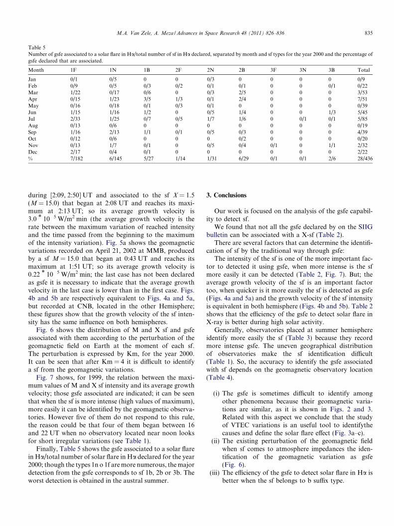
Table 5Number of gsfe associated to a solar flare in Ha/total number of sf in Ha declared, separated by month and sf types for the year 2000 and the percentage ofgsfe declared that are associated.

Month 1F 1N 1B 2F 2N 2B 3F 3N 3B Total

Jan 0/1 0/5 0 0 0/3 0 0 0 0 0/9Feb 0/9 0/5 0/3 0/2 0/1 0/1 0 0 0/1 0/22Mar 1/22 0/17 0/6 0 0/3 2/5 0 0 0 3/53Apr 0/15 1/23 3/5 1/3 0/1 2/4 0 0 0 7/51May 0/16 0/18 0/1 0/3 0/1 0 0 0 0 0/39Jun 1/15 1/16 1/2 0 0/5 1/4 0 0 1/3 5/45Jul 2/33 1/25 0/7 0/5 1/7 1/6 0 0/1 0/1 5/85Aug 0/13 0/6 0 0 0 0 0 0 0 0/19Sep 1/16 2/13 1/1 0/1 0/5 0/3 0 0 0 4/39Oct 0/12 0/6 0 0 0 0/2 0 0 0 0/20Nov 0/13 1/7 0/1 0 0/5 0/4 0/1 0 1/1 2/32Dec 2/17 0/4 0/1 0 0 0 0 0 0 2/22% 7/182 6/145 5/27 1/14 1/31 6/29 0/1 0/1 2/6 28/436

M.A. Van Zele, A. Meza / Advances in Space Research 48 (2011) 826–836 835

during [2:09, 2:50] UT and associated to the sf X = 1.5(M = 15.0) that began at 2:08 UT and reaches its maxi-mum at 2:13 UT; so its average growth velocity is3.0 * 10�5 W/m2 min (the average growth velocity is therate between the maximum variation of reached intensityand the time passed from the beginning to the maximumof the intensity variation). Fig. 5a shows the geomagneticvariations recorded on April 21, 2002 at MMB, producedby a sf M = 15.0 that began at 0:43 UT and reaches itsmaximum at 1:51 UT; so its average growth velocity is0.22 * 10�5 W/m2 min; the last case has not been declaredas gsfe it is necessary to indicate that the average growthvelocity in the last case is lower than in the first case. Figs.4b and 5b are respectively equivalent to Figs. 4a and 5a,but recorded at CNB, located in the other Hemisphere;these figures show that the growth velocity of the sf inten-sity has the same influence on both hemispheres.

Fig. 6 shows the distribution of M and X sf and gsfeassociated with them according to the perturbation of thegeomagnetic field on Earth at the moment of each sf.The perturbation is expressed by Km, for the year 2000.It can be seen that after Km = 4 it is difficult to identifya sf from the geomagnetic variations.

Fig. 7 shows, for 1999, the relation between the maxi-mum values of M and X sf intensity and its average growthvelocity; those gsfe associated are indicated; it can be seenthat when the sf is more intense (high values of maximum),more easily it can be identified by the geomagnetic observa-tories. However five of them do not respond to this rule,the reason could be that four of them began between 16and 22 UT when no observatory located near noon looksfor short irregular variations (see Table 1).

Finally, Table 5 shows the gsfe associated to a solar flarein Ha/total number of solar flare in Ha declared for the year2000; though the types 1n o 1f are more numerous, the majordetection from the gsfe corresponds to sf 1b, 2b or 3b. Theworst detection is obtained in the austral summer.

3. Conclusions

Our work is focused on the analysis of the gsfe capabil-ity to detect sf.

We found that not all the gsfe declared by on the SIIGbulletin can be associated with a X-sf (Table 2).

There are several factors that can determine the identifi-cation of sf by the traditional way through gsfe:

The intensity of the sf is one of the more important fac-tor to detected it using gsfe, when more intense is the sfmore easily it can be detected (Table 2, Fig. 7). But; theaverage growth velocity of the sf is an important factortoo, when quicker is it more easily the sf is detected as gsfe(Figs. 4a and 5a) and the growth velocity of the sf intensityis equivalent in both hemisphere (Figs. 4b and 5b). Table 2shows that the efficiency of the gsfe to detect solar flare inX-ray is better during high solar activity.

Generally, observatories placed at summer hemisphereidentify more easily the sf (Table 3) because they recordmore intense gsfe. The uneven geographical distributionof observatories make the sf identification difficult(Table 1). So, the accuracy to identify the gsfe associatedwith sf depends on the geomagnetic observatory location(Table 4).

(i) The gsfe is sometimes difficult to identify amongother phenomena because their geomagnetic varia-tions are similar, as it is shown in Figs. 2 and 3.Related with this aspect we conclude that the studyof VTEC variations is an useful tool to identifythecauses and define the solar flare effect (Fig. 3a–c).

(ii) The existing perturbation of the geomagnetic fieldwhen sf comes to atmosphere impedances the iden-tification of the geomagnetic variation as gsfe(Fig. 6).

(iii) The efficiency of the gsfe to detect solar flare in Ha isbetter when the sf belongs to b suffix type.

836 M.A. Van Zele, A. Meza / Advances in Space Research 48 (2011) 826–836

So, some of these inconveniences can be avoided if thedistribution of the observatories is improved and the iden-tification of a sf is made using simultaneously gsfe, solarwind parameters and isfe.

We can conclude that considering the last 9 years, theefficiency of the observation of a sf according to the geo-magnetic registration is low just now: 43% for X, 13% forM, 0.4% for C, and negligible for B and A.

In a further work we will improve our analysis includ-ing extreme ultra violet solar radiation monitored bysatellite.

Acknowledgements

The authors are very grateful to world data centersfor the free availability of the data: WDC-C KyotoUniversity, Japan; Service International des IndicesGeomagnetiques, Bureau des Publications SIIG, France;Consejo Nacional de Investigaciones Cientıficas yTecnicas, Argentina; Facultad de Ciencias Exactas yNaturales (Universidad de Buenos Aires), Argentina;and Facultad de Ciencias Astronomicas y Geofısicas(Universidad Nacional de La Plata), Argentina.

References

Baker, D.N. Effects of the Sun on the Earth’s environment. Journal ofAtmospheric and Solar-Terrestrial Physics 62 (17–18), 1669–1681,2000.

Ciraolo, L., Azpilicueta, F., Brunini, C., Meza, A., Radicella, S.M.Calibration errors on experimental slant total electron contentdetermined with GPS. Journal of Geodesy, 111–120, doi:10.1007/s00190-006-0093-1, 2007.

Curto, J.J., Gaya-Piquet, L.R. Geoeffectiveness of solar flares inmagnetic crochet (sfe) production: I-Dependence on their spectralnature and position on the solar disk. Journal of Atmospheric andSolar-Terrestrial Physics 71, 1695–1704, 2009.

Echer, E., Gonzalez, W.D., Guarnieri, F.L., Dal Lago, A., Vieira, L.E.A.Introduction to space weather. Advances in Space Research 35 (5),855–865, 2005.

IAGA Bulletin No. 12 l; 1961; Geomagnetic Data 1957. Indices K and C,Rapid Variations by Bartels, J., Romana, A., Veldkamp, J. IUGG,1957.

Mannucci, A.J., Tsurutani, B.T., Abdu, M.A., Gonzalez, W.D., Komjathy,A., Echer, E., Iijima, B.A., Crowley, G., Anderson, D. Superposed epochanalysis of the dayside ionospheric response to four intense geomagneticstorms. Journal of Geophysical Research 113, A00A02, doi:10.1029/2007JA012732, 2008.

Menvielle, M., Berthellier, A. The K derived planetary indices: descriptionand availability. Reviews of Geophysics 29 (3), 415–432, 1991.

Meza, A., Van Zele, M.A., Rovira, M. Solar flare effect on thegeomagnetic field and ionosphere. Journal of Atmospheric andSolar-Terrestrial Physics 71, 1322–1332, 2009.

Rastogi, R.G. Storm sudden commencements in geomagnetic H, Y and Zfields at the Equatorial Electrojet Station, Annamalainagar. Journal ofAtmospheric and Solar-Terrestrial Physics 60, 1295–1302, 1998.

Siscoe, G. The space-weather enterprise: past, present, and future.Journal of Atmospheric and Solar-Terrestrial Physics 62 (14),1223–1232, 2000.

SIIG bulletin mensuel, published by the Federation des services danalyse dedonnees astronomiques et geophysiques. Service international desindices geomagnetiques, France.

Tsurutani, B.T., Judge, D.L., Guarnieri, F.L., Gangopadhyay, P., Jones,A.R., Nuttall, J., Zambon, G.A., Didkovsky, L., Mannucci, A.J.,Iijima, B., Meier, R.R., Immel, T.J., Woods, T.N., Prasad, S., Floyd,L., Huba, J., Solomon, S.C., Straus, P., Viereck, R. The October 28,2003 extreme EUV solar flare and resultant extreme ionosphericeffects: comparison to other Halloween events and the Bastille Dayevent. Geophysical Research Letters 32, L03S09, doi:10.1029/2004GL021475, 2005.

Tsurutani, B.T., Verkhoglyadova, O.P., Mannucci, A.J., Saito, A., Araki,T., Yumoto, K., Tsuda, T., Abdu, M.A., Sobral, J.H.A., Gonzalez,W.D., Mc Creadie, H., Lakhina, G.S., Vasyliunas, V.M. Promptpenetration electric fields (PPEFs) and their ionospheric effects duringthe great magnetic storm of 30-31 October. Journal of GeophysicalResearch Letter 113, A05311, doi:10.1029/2007JA012879, 2008.

Van Sabben, D. Ionospheric current systems of the IGY. Solar flareeffects. Journal of Atmospheric and Terrestrial Physics 22 (1), 32–42,1961.

Voland, H., Taubenheim, J. On the ionospheric current system of thegeomagnetic solar flare effect (sfe). Journal of Atmospheric andTerrestrial Physics 12, 308–315, 1958.