doi.org/10.26434/chemrxiv.12133023.v1

Revealing Hidden Debottlenecking Potential in Flare Systems onOffshore Facilities Using Dynamic Simulations -- a PreliminaryInvestigationAna Xiao Outomuro Somozas, Rudi P. Nielsen, Marco Maschietti, Anders Andreasen

Submitted date: 15/04/2020 • Posted date: 20/04/2020Licence: CC BY-NC-ND 4.0Citation information: Somozas, Ana Xiao Outomuro; Nielsen, Rudi P.; Maschietti, Marco; Andreasen, Anders(2020): Revealing Hidden Debottlenecking Potential in Flare Systems on Offshore Facilities Using DynamicSimulations -- a Preliminary Investigation. ChemRxiv. Preprint.https://doi.org/10.26434/chemrxiv.12133023.v1

Three flare systems are modeled and total plant depressurization is investigated using dynamic simulations inorder to access the debottlenecking potential. Usually steady-state simulation of the flare network is used forsizing and rating of the flare system. By using dynamic simulations effects from line packing in the flare systemcan be studied. The results show that peak flow during a dynamic simulations is significantly lower than thepeak flow used in a steady-state case.The three systems investigated span a wide range in flare system size, both in terms of number of processsegments disposing into the flare network, in terms of peak design rate and the flare network pipe dimensionsand total hold-up volume. Generally, it is observed that the larger the flare system, the larger debottleneckingpotential.

File list (1)

download fileview on ChemRxivandreasen_et_al_2020.pdf (1.12 MiB)

Revealing hidden debottlenecking potential in flare

systems on offshore facilities using dynamic simulations

– A preliminary investigation

Ana Xiao Outomuro Somozasa, Rudi P. Nielsena, Marco Maschiettia,Anders Andreasenb,∗,

aAalborg University, Department of Chemistry and Bioscience, Niels Bohrs Vej 8,DK-6700 Esbjerg, Denmark

bRamboll Energy, Field Development, Studies and FEED, Bavnehøjvej 5, DK-6700Esbjerg, Denmark

Abstract

Three flare systems are modeled and total plant depressurization is inves-tigated using dynamic simulations in order to access the debottleneckingpotential. Usually steady-state simulation of the flare network is used forsizing and rating of the flare system. By using dynamic simulations effectsfrom line packing in the flare system can be studied. The results show thatpeak flow during a dynamic simulations is significantly lower than the peakflow used in a steady-state case. The three systems investigated span a widerange in flare system size, both in terms of number of process segments dis-posing into the flare network, in terms of peak design rate and the flarenetwork pipe dimensions and total hold-up volume. Generally, it is observedthat the larger the flare system, the larger debottlenecking potential.

Keywords: Emergency depressurization, Flare network, Debottlenecking,Dynamic simulation

∗Corresponding authorEmail address: anra@ramboll.com (Anders Andreasen)

Preprint submitted to Elsevier April 15, 2020

1. Introduction

The flare system is a pivotal part of the safety system in process plantshandling flammable and hazardous substances. In case of an upset conditioncausing for instance pressure relief or plant depressurization, the flare systemcollects vented substances and routes the hazardous fluids to the flare stack.At the flare tip incineration takes places, thereby converting the flammableand hazardous substances to less harmful oxidized products such as CO2

and H2O. The flare system boundaries are pressure safety valves (PSVs),emergency depressurization valves (EDPs)/blowdown valves (BDVs), spill-over valves/pressure control valves (PCVs), in one end, and the flare stack/tipin the other end. From each source, fluid is collected via tail pipes in anetwork of sub-headers, and headers, via a flare knock-out (KO) drum, tothe flare stack and flare tip.

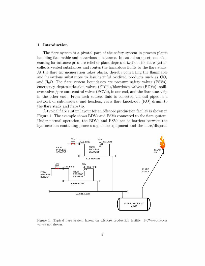
A typical flare system layout for an offshore production facility is shown inFigure 1. The example shows BDVs and PSVs connected to the flare system.Under normal operation, the BDVs and PSVs act as barriers between thehydrocarbon containing process segments/equipment and the flare/disposal

Figure 1: Typical flare system layout on offshore production facility. PCVs/spill-overvalves not shown.

2

Tail pipe Sub-header/header

Reference Mach. No. (–) ρv2 (Pa) Mach. No. (–) ρv2 (Pa)

API (2014) N/A N/A N/A N/ANORSOK (2014) 0.7 200,000 0.6 200,000Total (2012) 0.7 150,000 0.7 150,000Shell (2010) <1 N/A <1/0.7 N/A

Table 1: Typical design criteria used for sizing of flare network piping according to recog-nized standards and major oil company standards.

system. In real systems, multiple BDVs and PSVs are connected to sub-headers and headers.

The design of the flare system often follows API 521 recommended prac-tice (API, 2014) or similar European standards (ISO, 2006; NORSOK, 2014)or more detailed and/or stringent company guidelines. The flare system isdesigned for a number of scenarios e.g., pressure relief from one source, orsimultaneous reliefs from a number of coincident sources, production flaringand emergency depressurization etc.

Common design criteria for the flare network are summarized in Table 1.Furthermore, during the design of the flare system, it shall also be verifiedthat the backpressure within the flare system does not exceed the designpressure of any part.

API 521 (API, 2014) specifically mentions dynamic simulations as ameans for refinement of disposal system design load by e.g., considering thatindividual relief loads may occur at different times (Nougues et al., 2010) andin general to determine the disposal system hydraulic performance. However,it is common industry practice to determine the flare system hydraulic capac-ity with a steady-state network solver. Typically, initial peak flows are usedfor hydraulic sizing of all tail pipes, sub-headers, flare KO drum and flarestack/tip using a commercial steady-state network solver. When evaluatingthe backpressure and flow rate/velocity in a steady-state approach, these aredetermined under the assumption that the entire flare system is subjectedto the peak flow at once. Especially considering emergency depressurization,a steady-state approach is conservative. Taking the dynamic nature of thedepressurization process into account, it can easily be comprehended thatdownstream segments in the flare system e.g. main header, flare KO drum

3

and flare tip will never be subjected to the maximum flow (Chakrabartyet al., 2016). In reality, the initial (peak) flow will rapidly decline owing tothe reduction in the upstream pressure and the build up of backpressure.The former is caused by the plant segments being depressurized, whereas thelatter is caused by the line packing, i.e., the gradual filling of the entire flaresystem. These combined effects would effectively smoothen out the peakflow.

It is common practice to use dynamic analysis when considering the de-pressurization of individual process segments for e.g. sizing of the flow ca-pacity of the BDV and/or downstream restriction orifice (Haque et al., 1990;Richardson and Saville, 1992; Haque et al., 1992; Biswas and Fischer, 2017;Leporini et al., 2018). The initial rate is used as input to a steady-state flarenetwork simulation. Even individual relief loads from various relief scenar-ios are analyzed using dynamic simulations (Singh et al., 2007; Firth, 2016;Bjerre et al., 2017; Andreasen et al., 2018). On the other hand, the analysisof the flare system as a whole is typically not subjected to dynamic analysis(Chen et al., 1992).

Andreasen (2014) modeled a sub-part of a flare system on an existingoffshore oil and gas production facility. By comparing the system load fromsteady-state and dynamic simulations, it was found that taking line packinginto account via dynamic simulation, the simulated flare tip mass flow ratewas 12% lower than the corresponding steady-state simulation.

Wasnik et al. (2018) studied the depressurization of 14 blowdown seg-ments into an offshore complex flare system. The initial flow from the BDVsegments was 545 MMSCFD. The result of a dynamic simulation was thatthe maximum rate into the flare KO drum was 532 MMSCFD and the maxi-mum load at the flare tip (located 1.8 km away and connected to the processfacility via a 42” pipeline) was reduced to 447 MMSCFD (18% reductionfrom initial BDV rate). In the same study, an extension of an existing facil-ity was also investigated. Dynamic simulations showed that the maximumbackpressure calculated during a full plant depressurization was reduced byapprox. 17% compared to steady-state simulation results.

Jo et al. (2020) studied a separator blocked-outlet scenario with multiplePSVs discharging into the flare system of an offshore process facility usingdynamic simulations. They found that substantial line sizing optimizationcould be obtained for most lines compared to a traditional steady-state ap-proach, thereby reducing CAPEX. However, it was also discovered that afew lines had to be increased in size when analyzed in dynamics due to high

4

Mach numbers.Although the literature on dynamic flare system modeling for full plant

emergency depressurization is sparse, there are clear indications that ex-isting flare systems designed using a steady-state approach have additionalullage which can be revealed by dynamic simulations. This is especiallyuseful when considering brownfield modifications to existing processing fa-cilities adding equipment that needs to be accommodated within an existingflare system when depressurized. Following a steady-state approach, addingadditional flare system load will probably result in bottlenecks in the flaresystem requiring expensive upgrades. On the other hand, a dynamic model-ing approach may elucidate hidden debottlenecking potential by an inherentover-capacity of the original flare system, thereby avoiding expensive flaresystem upgrades. Dynamic modeling analysis have to be done case by case,since flare systems on different facilities are unique

In this paper, the hidden debottlenecking potential in flare systems onoffshore processing facilities is studied using dynamic simulations of the emer-gency depressurization event.

Three facilities in different sizes in terms of flare system design load andnumber of segments being depressurized are studied in an attempt to quantifyexpected built-in ullage. To the authours knowledge, this is the first studyreported, which systematically investigates the potential of applying dynamicsimulations for revealing hidden debottlenecking potential in existing flaresystems.

2. Methods

2.1. Tools and modeling

All simulations in the present study are conducted with Aspen HYSYSDynamics ver. 9 (AspenTech, Bedford, Massachusetts, USA). The processfluids are modeled using the Peng-Robinson equation of state (Peng andRobinson, 1976) and the COSTALD method is applied for liquid density(Hankinson and Thomson, 1979). Heavy hydrocarbon fractions are modeledas hypotheticals/pseudo-components.

The blowdown segment is modeled as a vessel in HYSYS with a volumeequivalent to the blowdown segment modeled. Heat transfer is not consideredin the present study, which means that the dimensions of the vessels usedfor modeling the blowdown segments are irrelevant, as long as the volume ismatched. The BDV for each blowdown segment is modeled as a control valve,

5

Figure 2: Example of blowdown segment modeling in HYSYS.

with a CV calibrated to the initial flow rate through the restriction orificedownstream the BDV. The CV is determined by the ANSI/ISA method (ISA,1995; Borden, 1998) using a semi-ideal Cp/Cv. The modeling of the blowdownsegments as a vessel and downstream BDV including restriction orifice (valveand orifice modeled as a control valve) is illustrated in Figure 2. The fluidcomposition for each blowdown segment is sourced from a correspondingsteady-state process simulation of the plant. The initial conditions are setaccording to the plant’s flare, blowdown and relief report. For blowdownsegments which extends over pressure change e.g. an entire compressor loop,the initial pressure before start of depressurization is found from a settle-outanalysis (Andreasen et al., 2015).

The flare network is modeled using details from existing Flare SystemAnalyser (FSA) (AspenTech, Bedford, Massachusetts, USA), which includespiping information about length an internal diameter. This information issourced and used for specifying equivalent HYSYS pipe segments. Fittingsdata from the equivalent FSA model is included in the HYSYS pipe segmentsexcept for swages.

The pipe segment in HYSYS has some shortcomings in its modeling rigore.g., acceleration pressure drop is not included for pure gas flow, which usesDarcy-Weisbach for pressure drop calculation. Still, we will use it for sim-plicity. It is the authors experience that this may lead to a slight under-estimation of backpressure with a resulting underestimation of line-packingeffect. The building of large networks with more rigorous tools, such ase.g. Aspen Hydraulics (AspenTech, Bedford, Massachusetts, USA), is verytedious.

6

Elevations of tail-pipes, sub-headers and headers are ignored, which isconsidered to have neglible influence ion the results. Only the contributionto static pressure drop from the elevation of the flare tip is included in themodel. The flare tip is modeled as a control valve with a CV calibrated tothe actual pressure drop at the design rate from vendor data.

2.2. System description

Three different flare systems on different offshore facilities are analyzedin the present study. A summary of key data describing the three systems isprovided in Table 2.

Design load No. BDVs Facility typeFacility (MMSCFD) (kg/h) (#) (IP/CPF)

A 73 88,000 13 IPB 341 350,000 24 IPC 714 684,000 43 CPF

Table 2: Summary of facilities flare systems investigated with dynamic simulations. IP:Integrated process facility with wellheads and processing facilities on the same topsidefacility. CPF: Central Processing Facility with bridge-connected platforms also referred toas shallow water complex. System volume is total piping and flare KO drum gas hold-upvolume.

2.3. Facility A

The first facility is an integrated platform designed for light crude withassociated gas, which has separation of oil, gas and water in a two-stageseparation train with final polishing of crude export in an electrostatic coa-lescer (final dewatering and desalting). A compression system boosts the gaspressure from the separators for wet gas export/reinjection and gas lift.

The system comprises a combined HP and LP flare system. The governinggas rate design capacity of the flare system is emergency depressurization.The main flare header is 16” and is routed to the Flare KO Drum. Thesize of the header is increased to 18” just upstream of the KO drum. A 14”flare line is routed from the KO drum (ID 3 m by T/T 10 m) to the flaretip. The flare system has 13 BDVs discharging into the flare system upondepressurization. The flare system as modeled in the process simulator isvisualized in Appendix A.

7

2.4. Facility B

Facility B is a gas-condensate integrated processing platform, with two-stage condensate knock-out and booster compression of flash-gas from the2nd stage separator. Before export, the gas is dehydrated and dew pointcontrolled (hydrocarbons).

The platform has separate LP and HP flare systems, but only the HPflare is modeled in the present study. The main flare header is 20” and isrouted to the flare KO drum. A 20” flare line is routed from the KO drum(ID 3 m by T/T Y m) to the flare stack/tip. The flare system has 24 BDVsdisposing into the flare system upon depressurization. The flare system asmodeled in the process simulator is visualized in Appendix B.

2.5. Facility C

The last facility modeled is a central processing facility handling produc-tion from a number of bridge-connected platforms including tie-backs fromremote facilities. Mainly gas condensate is handled and oil/water/gas sepa-ration is performed on the CPF including gas compression dehydration andhydrocarbon dew-pointing. The CPF exports gas to shore as well as it pro-vides gas lift to wells requiring artificial lift.

The flare system includes both an LP and HP flare system, but only theHP flare system is modeled. The HP flare system has separate 18” mainheaders for cold and warm (wet) flare terminating at the flare KO drum (ID3.55 m x T/T 10.6 m). A 24” flare line is routed from the KO drum to theflare stack/tip. The flare system has 43 BDVs disposing into the flare systemupon depressurization. The flare system as modeled in the process simulatoris visualized in Appendix C.

3. Results and Discussion

3.1. Facility A

For facility A, the emergency depressurization process is simulated usingthe dynamic process model depicted in Figure A.10 in Appendix A. Twosimulations are conducted; The first uses a fixed pressure boundary upstreamall BDVs at the value of the initial pressure prior to blowdown and thedynamic simulation is run until steady-state is reached. This relates to theapproach applied when using a steady-state network solver, where the peakflow is used.

8

0.0

0.5

1.0

1.5

2.0

2.5

3.0

0 1 2 3 4 5 6 7 8 9 10 11 12 13 14 15

Pre

ssure

(bar)

Time (min)

Subheader 1 Subheader 2 Subheader 3Header 1 Header 2 KO inFlare in Flare out

0.0

0.5

1.0

1.5

2.0

2.5

3.0

0 1 2 3 4 5 6 7 8 9 10 11 12 13 14 15

Pre

ssu

re (

bar)

Time (min)

Subheader 1 Subheader 2 Subheader 3Header 1 Header 2 KO inFlare in Flare out

(A) (B)

Figure 3: Comparison between calculated backpressure in selected flare lines, flare KOdrum for (A) steady-state and (B) dynamic simulations for facility A.

The second applies a zero flow boundary at the inlet of the blowdownsegments i.e. the pressure decreases with time in the blowdown segmentsconcurrently with the mass flow out of the blowdown valve/orifice. This sim-ulates the real dynamic behavior of the system with mass flow from blowdownsegment decreasing with time as the pressure upstream decreases.

In Figure 3, the backpressure in various places in the flare system, cal-culated using the steady-state approach and the full dynamic approach, aredepicted. As seen from the results, the peak backpressure with the dynamicapproach is lower than the corresponding steady-state value. This behavioris similar to the one observed by Wasnik et al. (2018).

The mass flow reaching the flare tip is also compared for the steady-state and dynamic simulations. This is shown in Figure 4. Included isalso a simulation run with a model with increased complexity, referred toas a dead ends model cf. A.11 in Appendix A. In this more complexmodel, all tail pipes and sub-headers from non-flow sources such as PSVs andPCVs which normally do not dispose into the flare system during emergencydepressurization have been included.

As seen from Figure 4, the mass flow rate in the dynamic simulations,both the with and without dead ends increases rapidly to a maximum value ata time between 0.5-1 min. after start of the depressurization. The maximummass flow rate is at a lower value than the steady-state value due to line-

9

0

10,000

20,000

30,000

40,000

50,000

60,000

70,000

80,000

90,000

100,000

0 1 2 3 4 5 6 7 8 9 10 11 12 13 14 15

Mass f

low

(kg/h

)

Time (min)

Steady State

Dynamics

Dead ends

(A)

87,165

75,795

73,171

65,000

70,000

75,000

80,000

85,000

90,000

Steady State Dynamics Dead ends

Mass flo

w (

kg/h

)

(B)

Figure 4: Comparison between calculated flare-tip mass flow for facility A for steady-state,dynamic simulations without dead ends, and dynamic simulations including dead ends.

10

0

1

2

3

4

5

6

7

8

9

10

11

12

0 1 2 3 4 5 6 7 8 9 10 11 12 13 14 15

Pre

ssure

(b

ar)

Time (min)

Header in Header out Subheader 5

Subheader 4 Subheader 3 Subheader 1

Subheader 2 Flare in Flare out

0

1

2

3

4

5

6

7

8

9

10

11

12

0 1 2 3 4 5 6 7 8 9 10 11 12 13 14 15

Pre

ssure

(bar)

Time (min)

Header in Header out Subheader 5

Subheader 4 Subheader 3 Subheader 1

Subheader 2 Flare in Flare out

(A) (B)

Figure 5: Comparison between calculated backpressure in selected flare lines, flare KOdrum for (A) steady-state and (B) dynamic simulations for facility B.

packing in the flare system in agreement with previous findings (Andreasen,2014; Wasnik et al., 2018). It is also noted that the peak mass flow is reducedby including the dead ends in the dynamic simulation model. The dead endscontribute with increased hold-up volume and hence a bigger line-packingpotential. The reduction in peak flare rate is 11,370 kg/h and 13,994 kg/hfor the dynamic model without and with dead ends, respectively. In relativenumbers, the reduction is 13% and 16%.

3.2. Facility B

For facility B, the emergency depressurization process is simulated usingthe dynamic process model depicted in Figure B.12 in Appendix B. Again,two simulations are conducted; a dynamic simulation run to a steady-stateusing the initial peak flow from blowdown segments and the full dynamicsimulation.

In Figure 5 the backpressures in various places in the flare system calcu-lated using the steady-state and the full dynamic approach are depicted. Asseen from the results, the peak backpressure with the dynamic approach islower than the corresponding steady-state value as also demonstrated for thefacility A model.

The mass flow reaching the flare tip is also compared for the steady-stateand dynamic simulations. This is shown in Figure 6. The results also include

11

a more complex model which includes all dead ends cf. B.13 in Appendix B.As seen from Figure 6, the mass flow in the dynamic simulations both the

one with and the one without dead ends increase rapidly to a maximum valueat a time between 0.5-1 min. after start of depressurization. The maximummass rate is at a lower value than the steady-state value as also shown forfacility A. Again, it is noted that the peak mass flow is reduced by includingthe dead ends in the dynamic simulation model. The reduction in peak flarerate is 41,670 kg/h and 44,329 kg/h for the dynamic model without andwith dead ends, respectively. In relative numbers, the reduction is 13.5%and 14.4%. Compared to facility A, the reduction in flare rate is higher inabsolute numbers for facility B, whereas the relative reduction is comparable.In absolute numbers, the inclusion of dead ends is very similar to Facility A,but less significant in relative numbers.

Combined with findings from facility A, the simulation results for facilityB suggest that it can be beneficial to build a simulation model including allsystem volumes. On the other hand, using a less complex model is conser-vative. Apparently, the larger facility B shows less reduction in flare rateby including dead ends as facility A. Although, not conclusive, this mightsuggest that a more accurate and detailed model is more important for asmaller facility.

In order to also assess the consequence of a dynamic simulation analysisof a flare system, on ρv2, one of the key design parameters, this is comparedbetween the steady-state model and the dynamic models without and withdead ends. Comparison is made between the peak values during dynamicsimulations and corresponding steady-state values for the main sub-headers,headers and main line to the flare tip in Figure 7.

As seen from Figure 7, the calculated peak ρv2 using the dynamic simu-lations is higher than the corresponding steady-state value for many of theinvestigated sub-headers and headers. Some are significantly exceeded e.g.Subheader 5 and Subheader 2 out. This phenomenon may be rationalized interms of a lower peak backpressure as illustrated in Figure 5 for the dynamicsimulations. A lower pressure results in lower density and hence larger ac-tual value flows, which translates to higher velocity. Although a lower densitycounterbalances a higher velocity, the velocity dominates since it is a squaredterm. Jo et al. (2020) also observed that in some flare lines, the Mach num-bers calculated in a dynamic simulation exceeded those from a steady-statesimulation.

This is an important takeaway when analyzing dynamic flare models,

12

0

50,000

100,000

150,000

200,000

250,000

300,000

350,000

0 1 2 3 4 5 6 7 8 9 10 11 12 13 14 15

Ma

ss f

low

(kg

/h)

Time (min)

Steady State

Dynamics

Dead ends

(A)

308,640

266,970264,311

260,000

270,000

280,000

290,000

300,000

310,000

320,000

Steady State Dynamics Dead ends

Ma

ss f

low

(kg

/h)

(B)

Figure 6: Comparison between calculated flare-tip mass flow for facility B for steady-state,dynamic simulations without dead ends and dynamic simulations including dead ends.

13

0

20,000

40,000

60,000

80,000

100,000

120,000ρ

v2

(kg/m

s2)

SS

DYN

DE

Figure 7: Comparison between calculated ρv2 Facility B for steady-state, dynamic simu-lations without dead ends, and dynamic simulations including dead ends.

and while lower mass flow rates and lower backpressure are important foridentifying spare capacity in the flare system, it is important also to analyzeother key design factors.

3.3. Facility C

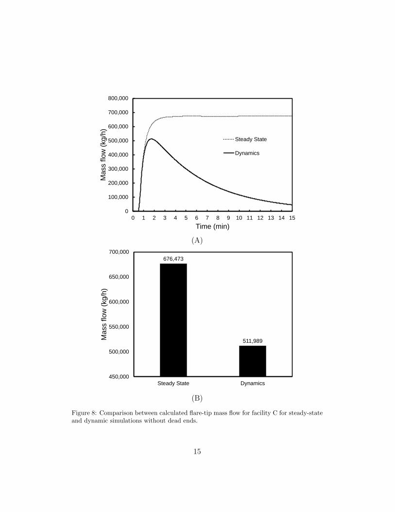
For facility C, the mass flow reaching the flare tip is compared for thesteady-state and dynamic simulations. This is shown in Figure 8.

As seen from Figure 8, the peak mass flow in the dynamic simulations isat a lower value than the steady-state value as also shown for facility A andB. The dynamic simulations results in a peak flare rate of 511,989 kg/h atthe flare tip compared to a steady-state value of 676,473 kg/h. The reductionin peak flare rate is 164,484 kg/h for the dynamic model which correspondsto a reduction of 24.3%. Compared to both facility A and B, the reductionin flare rate for facility C is higher in both absolute numbers and in relativenumbers. In absolute numbers, the order of reduction in peak flare rate isthe following A < B < C.

3.4. Synthesis

The results from the analysis of all three facilities are summarized in Table3. The main results are the steady-state design rate and the corresponding

14

0

100,000

200,000

300,000

400,000

500,000

600,000

700,000

800,000

0 1 2 3 4 5 6 7 8 9 10 11 12 13 14 15

Mass f

low

(kg/h

)

Time (min)

Steady State

Dynamics

(A)

676,473

511,989

450,000

500,000

550,000

600,000

650,000

700,000

Steady State Dynamics

Mass f

low

(kg/h

)

(B)

Figure 8: Comparison between calculated flare-tip mass flow for facility C for steady-stateand dynamic simulations without dead ends.

15

Peak flare rateLnet Vpipe VKO Vtot Dmean SS Dyn. Hidden potential

Facility Dead end (m) (m3) (m3) (m3) (inch) (MMSCFD) (MMSCFD) (%)

A no 288 19.2 79.4 98.6 10.5 72.8 63.2 9.5 13.0yes 497 27.0 79.4 106.4 9.3 72.8 61.1 11.7 16.1

B no 1,457 126 50.5 176.6 11.7 303.1 262.2 40.9 13.5yes 2,034 150 50.5 200.5 10.7 303.1 259.5 43.5 14.4

C no 2,686 359.6 103.3 462.9 15.3 733.2 555.0 178.2 24.3

Table 3: Summary of model details and modeling results for all three investigated facilities.Results included for models without and with dead ends included. Lnet: Total length ofpiping included in the flare network model, Vpipe: Hold-up volume of modeled piping, VKO:Hold-up volume of flare Knock-out drum, Vtot: Total hold-up volume of flare system,Dmean: Average diameter of flare network piping, found from a weighted average withindividual piping diameters weighted by their corresponding pipe length.

peak flare rate at the flare tip as found from a dynamic simulation of theemergency depressurization process. More specifically the difference betweenthe steady-state and dynamic analysis, also termed the hidden potential fordebottlenecking is included. Further, included are also details about the flaresystem in terms of hold-up volumes, flare network length and average flarepiping diameter.

It is seen from Table 3, that generally the total system volume of theflare system including both piping and the flare KO drum scales with thesteady-state design rate, which is partly due the average piping diameterbeing larger and partly due to longer piping in the flare system. This canbe rationalized by the fact that a larger design rate typically comes from ahigher number of blowdown segments, which in turn also comes from a largerfacility and hence longer piping.

It is also seen that a larger design rate also results in a higher potentialfor debottlenecking, especially considering the absolute value of the hiddenpotential. In relative terms, facility A and B are quite similar, with facilityC displaying a higher relative reduction in flare rate from dynamic analysis.

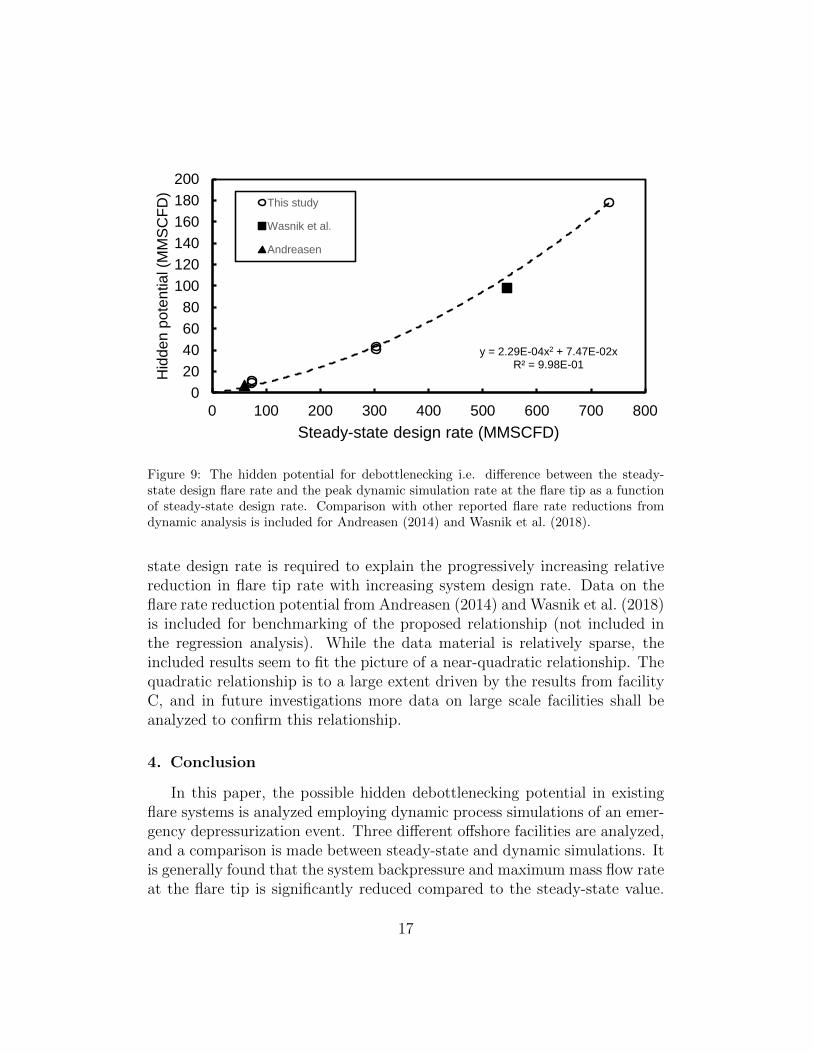
The difference between the steady-state design rate and the peak ratefound from dynamic simulations of the emergency depressurization for allinvestigated facilities is depicted as a function of the steady-state design ratein Figure 9.

In Figure 9, a second-order polynomial regression with a forced interceptat zero is also included which seems to fit the data from the present studyquite well. The quadratic dependence of the hidden potential on the steady-

16

y = 2.29E-04x2 + 7.47E-02xR² = 9.98E-01

0

20

40

60

80

100

120

140

160

180

200

0 100 200 300 400 500 600 700 800

Hid

de

n p

ote

ntia

l (M

MS

CF

D)

Steady-state design rate (MMSCFD)

This study

Wasnik et al.

Andreasen

Figure 9: The hidden potential for debottlenecking i.e. difference between the steady-state design flare rate and the peak dynamic simulation rate at the flare tip as a functionof steady-state design rate. Comparison with other reported flare rate reductions fromdynamic analysis is included for Andreasen (2014) and Wasnik et al. (2018).

state design rate is required to explain the progressively increasing relativereduction in flare tip rate with increasing system design rate. Data on theflare rate reduction potential from Andreasen (2014) and Wasnik et al. (2018)is included for benchmarking of the proposed relationship (not included inthe regression analysis). While the data material is relatively sparse, theincluded results seem to fit the picture of a near-quadratic relationship. Thequadratic relationship is to a large extent driven by the results from facilityC, and in future investigations more data on large scale facilities shall beanalyzed to confirm this relationship.

4. Conclusion

In this paper, the possible hidden debottlenecking potential in existingflare systems is analyzed employing dynamic process simulations of an emer-gency depressurization event. Three different offshore facilities are analyzed,and a comparison is made between steady-state and dynamic simulations. Itis generally found that the system backpressure and maximum mass flow rateat the flare tip is significantly reduced compared to the steady-state value.

17

This is due to line-packing effects in the flare system hold-up volume andthe fact that the mass flow decreases rapidly as the blowdown segments aredepressurized.

By comparing different model complexities, it is also shown that a higherdebottlenecking potential can be revealed, if dead ends from non-flow sourcesare included, since this increases the available hold-up volume. However, theeffect is not the dominating one, and can be ignored for more conservativeresults, especially when fast screening studies are required.

While both mass rates and back pressure decrease, it is observed that insome locations in the flare system the ρv2 may actually increase in a dynamicsimulation. This can be explained by lower backpressure and hence higherpeak velocity due to a lower gas density.

By compiling and analyzing the results for all three facilities, apparentlyit is found that the larger the facility, the larger the debottlenecking poten-tial. A quadratic relationship between the flare system design rate and thecorresponding debottlenecking potential fits the data well.

18

Appendix A. Facility A flare network

19

Figure A.10: Flare system model for facility A. Dead ends from PSVs and PCVs notdisposing into the flare system during emergency depressurization have not been included.

20

Figure A.11: Flare system model for facility A. Dead ends from PSVs and PCVs notdisposing into the flare system during emergency depressurization have been included.

21

Appendix B. Facility B flare network

22

Figure B.12: Flare system model for facility B. Dead ends from PSVs and PCVs notdisposing into the flare system during emergency depressurization have not been included.

23

Figure B.13: Flare system model for facility B. Dead ends from PSVs and PCVs notdisposing into the flare system during emergency depressurization have been included.

24

Appendix C. Facility C flare network

25

Figure C.14: Flare system model for facility C. Dead ends from PSVs and PCVs notdisposing into the flare system during emergency depressurization have not been included.

26

Abbreviations and symbols

Dmean Average diameter of flare network piping

Lnet Total length of piping included in the flare network model

VKO Hold-up volume of flare Knock-out drum

Vpipe Hold-up volume of modeled piping

Vtot Total hold-up volume of flare system

Cp Specific heat capacity at constant pressure

Cv Specific heat capacity at constant volume

API American Petroleum Institute

BDV Blowdown Valve

CV Valve flow coefficient

CPF Central Processing Facility

DE Dead end

Dyn. Dynamic (simulation)

EDP Emergency Depressurization

FSA Flare System Analyzer

HP High-Pressure

ID Internal diameter

IP Integrated process facility

KO Knock-out

LP Low-Pressure

NORSOK NORsk SOkkels Konkurranseposisjon

PCV Pressure Control Valve/Spill-over valve

27

PSV Pressure Safety Valve

SS Steady-state

T/T Tan-to-tan

References

Andreasen, A., 2014. Process design – can we change mindset?, in: OffshoreOil and Gas seminar, 18-22 August 2014, Department of Energy Technol-ogy, Aalborg University Esbjerg. doi:10.13140/RG.2.2.13310.33606. oralpresentation.

Andreasen, A., Borroni, F., Zan Nieto, M., Stegelmann, C., P. Nielsen,R., 2018. On the Adequacy of API 521 Relief-Valve Sizing Methodfor Gas-Filled Pressure Vessels Exposed to Fire. Safety 4, 11.doi:10.3390/safety4010011.

Andreasen, A., Eriksen, J.G.I., Stegelmann, C., Lynggaard, H., 2015.Method improves high-pressure settle-out calculations. Oil & Gas Journal113, 88–96.

API, 2014. Pressure-relieving and Depressuring Systems, API Standard 521.Technical Report API Standard 521, Sixth Edition, January. AmericanPetroleum Institute.

Biswas, S., Fischer, B.J., 2017. Application and validation of the apianalytical fire method in pressure-relieving and depressuring systems.Journal of Loss Prevention in the Process Industries 50, 154 – 164.doi:10.1016/j.jlp.2017.09.008.

Bjerre, M., Eriksen, J.G.I., Andreasen, A., Stegelmann, C., Mandø, M., 2017.Analysis of pressure safety valves for fire protection on offshore oil and gasinstallations. Process Safety and Environmental Protection 105, 60–68.doi:10.1016/j.psep.2016.10.008.

Borden, G. (Ed.), 1998. Control Valves – Practical Guides for Measurementand Control. Instrument Society of America.

Chakrabarty, A., Mannan, S., Cagin, T., 2016. Multiscale Model-ing for Process Safety Applications. Butterworth-Heinemann, Boston.doi:10.1016/B978-0-12-396975-0.05001-4.

28

Chen, F.F.K., Jentz, R.A., Williams, D.G., 1992. Flare System Design: ACase for Dynamic Simulation, in: Offshore Technology Conference, pp.421–430. doi:10.4043/6919-MS.

Firth, B., 2016. Unpicking Oversimplification: Relief and Flare Studies forComplex Plant using Dynamic Process Modelling, in: Hazards 26, Insti-tution of Chemical Engineers Symposium Series, pp. 1–12.

Hankinson, R.W., Thomson, G.H., 1979. A new correlation for saturateddensities of liquids and their mixtures. AIChE Journal 25, 653–663.doi:10.1002/aic.690250412.

Haque, A., Richardson, S., Saville, G., Chamberlain, G., 1990. Rapid depres-surization of pressure vessels. Journal of Loss Prevention in the ProcessIndustries 3, 4 – 7. doi:10.1016/0950-4230(90)85015-2.

Haque, M.A., Richardson, M., Saville, G., 1992. Blowdown of pressure ves-sels. Pt. I: Computer model. Trans. IChemE B 70, 3–9.

ISA, 1995. Flow Equations for Sizing Control Valves, ANSI/ISA S75.01Standard, ISA-S75.01-1985 (R 1995). Instrument Society of America.

ISO, 2006. Petroleum, petrochemical and natural gas industries — Pressure-relieving and depressuring systems . Technical Report ISO 23251:2006(E).International Organization for Standardization.

Jo, Y.P., Cho, Y., Hwang, S., 2020. Dynamic analysis and op-timization of flare network system for topside process of offshoreplant. Process Safety and Environmental Protection 134, 260 – 269.doi:10.1016/j.psep.2019.12.008.

Leporini, M., D’Alessandro, V., Mancini, E., Terenzi, A., Marchetti, B.,Giacchetta, G., Grifoni, R.C., 2018. A new integrated approach to studythe thermal and mechanical response of vessels subject to a safe blowdownprocess. Journal of Loss Prevention in the Process Industries 53, 103 – 114.doi:10.1016/j.jlp.2017.06.003. risk Analysis in Process Industries: State-of-the-art and the Future.

NORSOK, 2014. Process System Design, NORSOK Standard, P-002, Edition 1, August 2014. Technical Report. NORSOK. URL:www.standard.no/petroleum.

29

Nougues, J., Gruber, D., Leipnitz, D.U., Sethuraman, P., Alos, M., Brodkorb,M., 2010. Are there alternatives to an expensive overhaul of a bottleneckedflare system? Petroluem Technology Quarterly Q1, 94.

Peng, D.Y., Robinson, D.B., 1976. A new two-constant equation ofstate. Industrial & Engineering Chemistry Fundamentals 15, 59–64.doi:10.1021/i160057a011.

Richardson, S.M., Saville, G., 1992. Blowdown of vessels and pipelines, in:Institution of Chemical Engineers Symposium Series, pp. 195–209.

Shell, 2010. Design of pressure relief, flare and vent systems, Shell DEP80.45.10.10. Shell.

Singh, A., Li, K., Lou, H.H., Hopper, J., Golwala, H., Ghumare, S., Kelly, T.,2007. Flare minimisation via dynamic simulation. International Journalof Environment and Pollution 29, 19–29. doi:10.1504/IJEP.2007.012794.

Total, 2012. GENERAL SPECIFICATION, PROCESS GS EP EP 103, Pro-cess Sizing Criteria, rev. 7. TOTAL.

Wasnik, R., Singh, H., Kamal, F.R., Takieddine, O.H., 2018. De-bottlenecking of existing flare system for facility up-gradation using dy-namic simulation approach - case study, in: Abu Dhabi InternationalPetroleum Exhibition & Conference, 12-15 November, Abu Dhabi, UAE,Society of Petroleum Engineers. pp. 1–12. doi:10.2118/192750-MS. paperSPE-192750-MS.

30

download fileview on ChemRxivandreasen_et_al_2020.pdf (1.12 MiB)