On the spatial scales of a river plume

James O’Donnell,1 Steven G. Ackleson,2 and Edward R. Levine3

Received 6 July 2007; revised 20 September 2007; accepted 8 January 2008; published 12 April 2008.

[1] We report observations of the structure of the front that surrounds the plume of theConnecticut River in Long Island Sound (LIS). Salinity, temperature, and velocity in thenear-surface waters were measured by both towed and ship-mounted sensors and anautonomous underwater vehicle. We find that the plume front extends south from themouth of the river, normal to the direction of the tidal flow in LIS and then curves to theeast to parallel the tidal current. The layer depth at the front and the cross-front jumps insalinity and near-surface velocity all tend to decrease as distance from the sourceincreases. This is qualitatively consistent with the prediction of layer models. In theacross-front direction, the plume layer depth increases from zero to the asymptotic valuewithin a few times the plume depth (�5 m). Vertical motion is generated in this zone, andthere is evidence of overturning. Farther from the front, the high-frequency salinitystandard deviation decays exponentially with a length scale of 30 m. Assuming that thesalinity fluctuations are a consequence of turbulence, we find that the rate of turbulentkinetic energy dissipation decreases exponentially in the across-front direction with adecay scale LG � 15 m. Estimates based on AUV-mounted shear probes are consistentwith this estimate. We present an explanation of the physics that determines LG andprovide a simple formula to guide the choice of resolution in models that are designed toresolve the frontal structure.

Citation: O’Donnell, J., S. G. Ackleson, and E. R. Levine (2008), On the spatial scales of a river plume, J. Geophys. Res., 113,

C04017, doi:10.1029/2007JC004440.

1. Introduction

[2] Since freshwater runoff transports particulates anddissolved material from land to estuaries and the coastalocean, a quantitative understanding of the mechanisms ofmixing and dispersion of this effluent is essential to im-proving our ability to predict and assess the consequencesof human activity in the coastal ocean. Observations havemade it clear that, during periods of high discharge, manyrivers form large plumes of brackish water on the adjacentinner continental shelf that are frequently bounded byfronts. Examples are described by Garvine [1974], Stronach[1977], Ingram [1981], Freeman [1982], Lewis [1984],Luketina and Imberger [1987], Geyer et al. [1998] andHickey et al. [1998]. A review of the earlier observations isgiven by O’Donnell [1993]. It is clear that the horizontalscales of variation at the fronts of river plumes can be assmall as a few meters and that the density change canexceed 10 sT [see O’Donnell, 1997; O’Donnell et al., 1998;Trump and Marmorino, 2002, 2003]. Though three dimen-sional primitive equation models are now being widelyemployed to simulate the exchange between rivers and theocean, as yet there have been none that resolve these small

scales. The efficient design of models that are capable ofeffectively predicting the dispersion of terrestrial runoff inthe coastal ocean requires that we establish the scales thatmust be resolved in the frontal boundaries and the processesthat control the rate of vertical mixing.[3] Recent technical advances in navigation and current

measurement now allow a more detailed examination of thestructure of plumes and plume fronts at the important spatialscales as shown by O’Donnell [1997], O’Donnell et al.[1998] and Trump and Marmorino [2002, 2003]. Here wedescribe the along-front variation of the pycnocline depthand the near-surface salinity and velocity on either side ofthe front. We also present the first quantitative estimates ofthe width of the frontal region in which mixing occurs andpresent estimates of the variation of the turbulent kineticenergy dissipation rate, e, within the frontal zone.

2. Frontal Structure and Plume Theories

[4] Garvine [1974] developed a two dimensional (verticaland horizontal) model of the structure of the density andflow field in small-scale fronts. In this model ‘‘small’’referred to the ratio of the horizontal length scale to theinternal deformation radius, and justified the neglect of theCoriolis acceleration. Garvine assumed the dynamic balancewas between the advection of momentum, the baroclinicpressure gradient and vertical eddy viscosity. He thenprescribed the density field and the spatial structure ofvertical mixing and friction across the base of the buoyantlayer and predicted the vertical and horizontal variation in

JOURNAL OF GEOPHYSICAL RESEARCH, VOL. 113, C04017, doi:10.1029/2007JC004440, 2008ClickHere

for

FullArticle

1Department of Marine Sciences, University of Connecticut, Groton,Connecticut, USA.

2Office of Naval Research, Arlington, Virginia, USA.3Naval Undersea Warfare Center, Newport, Rhode Island, USA.

Copyright 2008 by the American Geophysical Union.0148-0227/08/2007JC004440$09.00

C04017 1 of 12

the velocity field. The magnitude of vertical mixing andfriction was assumed to decay exponentially with distancefrom the front with a length scale, LG, that was unknown.The model allowed an exploration of the influence of LG onthe structure of the frontal circulation and Garvine thenestimated the value that allowed qualitative agreementbetween the predictions and the observations of Garvineand Monk [1974]. O’Donnell et al. [1998] obtained muchhigher resolution measurements of the density and velocityfields and demonstrated that LG had to be much smaller thanGarvine [1974] reported. In this paper we present the firstmeasurements that allow direct estimates of LG.[5] The observations that fronts have much smaller spa-

tial scale than plumes was exploited in the models ofGarvine [1982] and O’Donnell [1988, 1990]. These modelsconsidered a plume to be a thin buoyant layer overlying adenser and much thicker ambient fluid layer. This allowedthe dynamics of the buoyant layer to be simulated by thenonlinear long wave equations with weak frictional cou-pling at the interface. The lower layer, though in motion,was assumed to be unaffected by the upper layer. Thefrontal boundary was assumed to have a very smallacross-front scale (compared to that of horizontal variationsin the plume) and modeled as a discrete line surrounding theplume layer. Exchange of mass and momentum was as-sumed to be significant in the frontal zone and weakelsewhere. For the special case of a straight linear frontwith no along-front velocity component, Garvine [1981]developed algebraic relationships between the layer thick-ness and velocity at the front and the rate of translation ofthe front relative to the ambient fluid. This approach isanalogous to the use of shock patching in compressible gasdynamics. Garvine’s frontal jump conditions, (the analog of

the Rankin-Hugoniot shock conditions) included twoparameters chosen with guidance from laboratory observa-tions. Mathematically, the problem is to determine theposition of the front and the solution to the long waveequations subject to specified inflow conditions and thefrontal jump conditions.[6] Garvine [1982] developed a technique to obtain a

numerical solution when the discharge and ambient velocitywere steady. The approach restricted the angle between thedischarge and the ambient flow for which solutions could beobtained. An example of the predicted interface depthdistribution is shown in Figure 1a. To reveal the structuremost clearly, the layer depth is plotted upward. The max-imum value occurs at the source where the layer depth andtransport are prescribed. Elsewhere, the maximum occurs atthe front and decreases in the offshore direction as the frontbends toward the ambient flow vector. In contrast, thenumerical technique employed by O’Donnell [1988, 1990]allowed unsteady behavior in both the source and ambientconditions but required cylindrical symmetry near thedischarge. An example solution for the expansion of aplume and the evolution of the layer depth structure witha steady discharge and cross flow and no interfacial ex-change in the interior is shown in Figures 1b–1e. Thesesolutions show the plume spreading into the ambient flowand becoming asymmetric as the cross flow arrests the fronton the upstream side (with respect to the cross flow) andaccelerates it on the downstream side. Consequently, theplume layer becomes thicker on the upstream side andthinner on the downstream side.[7] The interior structure of the plume layer thickness is

quite different in Figures 1a and 1e with a shallow troughevident between the source and the front in the radial

Figure 1. (a) A-three dimensional projection of the layer depth (plotted as a positive upward) predictedby the model of Garvine [1982] for a plume discharged from a channel into a steady cross flow. Note thatthe depth at the front decreases with distance from the source as the front bends toward the direction ofthe along-coast flow velocity vector. (b–e) The evolution of the interfacial depth and horizontal transportvectors in a spreading plume from a cylindrically symmetric source in a uniform cross flow predicted bythe model of O’Donnell [1988]. The initial condition, t = 0.45, is shown in Figure 1b, and solutionscomputed at times t = 1.04, 2.00 and t = 3.74 are presented in Figures 1c–1e. Though the dischargegeometry is quite different, the front expands into and across the ambient flow with the depth at the frontdecreasing in the along front direction with distance from the source.

C04017 O’DONNELL ET AL.: SPATIAL SCALES OF A RIVER PLUME

2 of 12

C04017

discharge example. This difference results from the differentsource geometries chosen to circumvent limitations imposedby the numerical solution techniques adopted by Garvine[1982] and O’Donnell [1988]. More importantly, the twomodels display common features that are not sensitive to thechoice of frontal parameters or source conditions including:(1) the angle between the frontal boundary and the ambientflow velocity vector decreases with distance along the front,and (2) the depth of the interface at the front decreases withdistance along-front from the source. In Figures 1b–1e,the front is almost normal to the ambient velocity near thedischarge and curves to become almost parallel to theambient flow further from the source. It is clear that thisfeature is consistent with Garvine’s [1974] observations ofthe Connecticut River plume structure. However, observa-tions are inadequate to conclude whether the predictedalong front depth variation is also valid.[8] Both models of Garvine [1982] and O’Donnell [1988]

imbedded the Garvine [1981] frontal conditions that as-sumed that the front was straight and the magnitude ofinterfacial mixing and friction was proportional to the front-normal component of the velocity of the underlying waterrelative to the front. The neglect of the vertical shear in thealong-front velocity in these models requires the front tospread across the ambient flow more rapidly than it would ifthe shear in the along front velocity enhanced verticalmixing and friction. These approximations were justifiedsince no laboratory or field observations were available toguide the development of a more appropriate parameteriza-tion. However, the prediction of the along-front variationremains untested.

3. Observations

[9] The structure of the Connecticut River plume frontwas examined on the morning of 27 April 2000 usinginstruments deployed from the R/V Connecticut. The windswere less than 5 m/s and the river discharge at the USGSstation at Thompsonville, CT, was 1,192 m3s�1, i.e., closeto the long-term average for April and more than twice themean annual discharge. The observations took place onthe latter half of the ebb tide in Long Island Sound whenthe work of Garvine [1974] suggests that the plume shouldbe to the east of the river mouth.[10] The velocity field and acoustic backscatter intensity

were measured by an RD Instruments 1.2 MHz BroadbandAcoustic Doppler current profiler (ADCP) mounted 0.7mbelow the surface on a vertical pipe attached to the side ofthe R/V Connecticut. The ship heading was acquired from aTrimble TANS Vector AGPS system at 10 Hz, filtered anddecimated to 1 Hz. The ship position was acquired from aTrimble Differential Global Positioning System (DGPS).The ADCP water and ship velocity estimates were acquiredat 1Hz and postprocessed to incorporate the AGPS headingdata and correct for variations in the speed of sound, a lessthan 2% effect. The uncertainty of the ADCP velocitymeasurements were evaluated by comparing the ship ve-locity estimated using the ADCP bottom track velocityaveraged in 20 s bins to that obtained from the DGPSpositions at the beginning and end of the averaging interval.The root mean square difference in the estimates was 10 cm/s.This is consistent with the error expected from the

navigation system when the ship is moving at approximate-ly 1 m/s. The fundamental uncertainty in the relativehorizontal velocity component estimates in 0.25 m verticalbins was 10 cm/s [RD Instruments, 1997].[11] The pressure, salinity and temperature were mea-

sured at 1Hz by an Ocean Sensors OS200 mounted next tothe ADCP transducers at 1 m below the surface on the portside of the vessel. The same variables were measured at 8 Hzby a Seabird 25 CTD mounted on a towed body (the BDF)and attached to a crane over the starboard side of the shipapproximately 2 m below the surface and 5 m astern of theADCP.[12] The most relevant observations were acquired begin-

ning at 10:30 EST when the tidal currents in LIS were nearmaximum ebb. At this time the river plume front was clearlydelineated by a line of white foam (see Figure 2) whichbegan at the southern end of the western breakwater at theriver mouth. The photograph in Figure 2 was taken lookingto the northwest and the front can be seen to trendsouthward from the breakwater and then curve to a morenortheast-southwest alignment. The foam patch in theforeground is approximately 1 m in width, and the meandersin the front have a wavelength of approximately 10 m, ingeneral agreement with the observations described byTrump and Marmorino [2002, 2003]. While samplingcontinuously, the R/V Connecticut steered a zig-zag trackthat crossed the front five times. Figure 3 shows a map ofthe coastline and bathymetry at the mouth of the Connect-icut River with the ship track indicated by the thick grayline. The position of the ship when it crossed the front areshown by the plus symbols. Note that the tidal flow in LISis to the east during the ebb which is to the right in Figure 3.This is not to be confused with the direction of the ambientcross flow assumed in the numerical solutions in Figures 1aand 1b–1e. During the 1994 observation campaign de-scribed by O’Donnell et al. [1998] the Connecticut Riverdischarge was approximately 1500 m3s�1 and the front wasapproximately 1 km to the west of the locations shown inFigure 3. Since it took almost an hour to complete the trackthe shape of the front in Figure 3 is not a synoptic view andno corrections have been applied to correct for the frontalvelocity. The times that the ship crossed the front are listedin Table 1 with the transects numbered in order of increas-ing distance from the river mouth and not by time.[13] After the ship surveys were completed, a REMUS

[von Alt et al., 1994] autonomous underwater vehicle (AUV)was deployed at the location labeled ‘‘Start’’ in Figure 3.The AUV then propelled itself at 1 m depth northeast atapproximately 1 m/s along the track shown by the solid lineusing an array of four acoustic navigation beacons. While theAUV was being configured and readied for deployment, thefront moved to the west and was oriented approximatelynorth–south when the AUV crossed it. The bow of theAUV was instrumented with turbulence and fine structuresensors as described by Levine and Lueck [1999]. Theinstrument suite included two-axis small-scale velocity shearprobes [Osborn and Crawford, 1982], ultra fast thermistorsto measure small-scale temperature and vertical temperaturegradient, and three orthogonal accelerometers for motioncompensation. In addition, the REMUS vehicle measuredthe vertical gradient of horizontal velocity using an upwardand downward looking 1200 kHz RDI ADCP, finescale

C04017 O’DONNELL ET AL.: SPATIAL SCALES OF A RIVER PLUME

3 of 12

C04017

temperature and salinity using a pair of FSI CTDs, andthree-dimensional small-scale velocity using a Sontek Acous-tic Doppler Velocimeter. The AUV-based instruments allowedthe calculation of the horizontal distribution of the turbulentkinetic dissipation rate, horizontal velocity shear, and thefine-scale stratification following the approach described byGoodman et al. [2006]. A comprehensive discussion of theREMUS observations is provided by Levine et al. [2008].In this report we only discuss the shear probe estimates ofthe distribution of the turbulent kinetic energy dissipationrate and compare them to the distribution inferred from theship-mounted instruments.[14] The six plots in Figure 4 show the variation of the

salinity measured by the ship-mounted CTD at 0.7 m depth(thin lines) and, when available, the towed BDF (thick lines)as functions of the across-front distance. The stratified waterof the river plume is on the right side of the plots and thehigher-salinity, and less stratified, water of LIS is to the left.The location of the horizontal position origin in each sectionis the position recorded by the R/V Connecticut’s navigationsystem at the time the ship mounted ADCP and CTDcrossed the foam line. In Figures 4a and 4d the salinityjumps occur a few meters from the origin owing to smallerrors in recording the times the front was crossed andoffsets between the position of the foam line and the salinityjump. At a survey speed of 2.5 m/s, a 2 second error inrecording the crossing time results in an offset of 5 m.[15] To estimate and correct the horizontal offset of the

ship-mounted and towed sensors we assume that theleading edge of the front is vertical and then computethe time lag between the salinity jumps in the two records.The BDF data is then offset to estimate the fields that wouldhave been observed had the instruments been aligned in thevertical as in work by O’Donnell et al. [1998]. The spatialuncertainty introduced by this approach is to be a meter ortwo. Since the horizontal gradients are small, except in theimmediate vicinity of the salinity jump, this error isinsignificant.

[16] The central feature of the 0.7 m level salinityobservations (labeled Su, in all six parts of Figure 4) isthe abrupt decrease in salinity that occurs at x = 0 in all sixtransects. With the exception of section 2, Figure 4b, theabrupt decrease in salinity is followed by a slow rise to anintermediate value. The magnitude of the near surfacesalinity jump generally decreases in the offshore direction,i.e., from section 1 to 6.[17] The salinity observations made by the BDF on

sections 1, 3, 4 and 5 (labeled SB in Figures 4a, 4c, 4d,and 4e) show similar structure to the 0.7 m level measure-ments though the faster sampling rate reveals high wavenumber variability that appears to have large amplitude nearthe front and to decay toward the plume. The lines labeledsB in Figure 4 show the standard deviation of the BDF

Figure 3. Ship track during sampling operations at theConnecticut River mouth on 27 April 2000. The dashedlines show bathymetric contours (m) and the location of thebreakwaters at the mouth of the Connecticut River. Thetrack of the R/V Connecticut is shown by the thick curvingsolid gray line. The locations where the ship crossed thefoam line of the front is shown by the plus symbols. Timesof the crossings are presented in Table 1. The orientation ofthe across- and along-front coordinate system used in theanalysis is shown by the arrows. The short line between the‘‘start’’ and ‘‘end’’ labels shows the transit of the turbulencemeasuring AUV.

Figure 2. Photograph of the river plume front at the mouthof the Connecticut River, taken on 27 April 2000, showingthe front curving toward the western breakwater and short(�10 m) along-front variations and foam patches in thecenter of small (�1 m) cyclonic vortices.

Table 1. Times at Which the Ship Crossed the Front

Section Front Crossing Time

1 09:532 10:173 09:464 09:425 09:386 09:33

C04017 O’DONNELL ET AL.: SPATIAL SCALES OF A RIVER PLUME

4 of 12

C04017

salinity in 2 s bins (16 samples) and demonstrate this pointmore clearly.[18] An example of the ADCP horizontal velocity obser-

vations from section 2 is presented in Figure 5. To reducethe noise to 3 cm/s the observations at �1 Hz were averagedin 3 s time bins and 0.75 m vertical bins and are presentedas functions of distance from the front in the local front-normal direction. The structure of the flow is very similar tothat described by O’Donnell et al. [1998] with the across-front velocity in Figure 5 directed to the left near the surfaceand to the right (toward and under the plume) everywhere

else. The mean-square shear, S2 ¼ du

dz

� �2

þdndz

� �2

, cor-

rected for the noise bias, is approximately 0.15 s�2 at2.25 m on sections 1 and 2.[19] Since the depth of the BDF is variable and the

structure of the plume front changes in the along-frontdirection, further interpretation of these observationsrequires that the BDF location relative to plume structurebe illustrated. It is well established theoretically and empir-ically [Seim, 1999] that the acoustic backscatter in the 1–103 kHz range is often dominated by salinity microstructurein estuarine waters. Deines [1999] outlined how ADCPmeasurements of backscatter signal strength can be cor-rected for losses due to absorption and beam spreading to

Figure 4. Salinity at 1m (labeled Su) and at the BDF depth (labeled SB), which we show in Figure 5.The distribution of the standard deviation of the salinity fluctuations measured by the BDF in 2-s timewindows are shown by the lines labeled sB.

Figure 5. (a) Across-front and (b) along-front velocity components measured by the ship-mounted1200-kHz ADCP on section 2 as a function of depth and across-front distance.

C04017 O’DONNELL ET AL.: SPATIAL SCALES OF A RIVER PLUME

5 of 12

C04017

obtain the vertical structure of backscatter intensity and thishas been implemented to create the across-front distributionof backscatter from the ship-mounted ADCP shown inFigure 6. Prior work in at the Connecticut River plumefront by O’Donnell et al. [1998] demonstrated the similarityof the structure of the acoustic backscatter distribution andthe plume thickness observed by a rigid array of salinitysensors. In Figure 6a the track of the BDF (the solid blackline) clearly goes through the high-backscatter region at theleading edge of the plume and then into the stratified layer.In section 2 the region of highest backscatter in the top 3 m(see Figure 6b) appears to be much wider than in section 1.Note that no BDF data was acquired on section 2. Onsections 3 and 4 the BDF passed through the lower edge ofthe high-backscatter layer and the salinity observations inFigures 4c and 4d confirm that the LIS water was appre-ciably diluted by freshwater at the level of the BDF. Incontrast, the salinity in Figures 4e and backscatter inFigure 6e agree that the BDF passed below the level ofthe plume on section 5. The 0.7 m salinity observationsshow that a very shallow, highly stratified plume layer waspresent at both sections 5 and 6 though the ADCP data andBDF measurements were too deep to resolve it.

4. Analysis

[20] The along front variation of the salinity in the plumeis presented using measurements averaged in 2.5 m hori-zontal bins on either side of the front at both the level of theCTD and the BDF. Figure 7 displays the variation of theseproperties with along-front distance from the breakwater at

the western side to the river mouth where the plume frontfirst appears well-organized. Comparison of the dashedlines shows the salinity difference across the front at the0.7 m level with the ‘O’ markers representing the salinity ofthe LIS water and the plus symbols showing the lowersalinity of the plume water. The variations in the LIS waterare relatively weak. In contrast, the near surface salinity ofthe plume increases offshore at a rate of approximately5 km�1. At 1600 m from the breakwater the salinity jumpacross the front near the surface is only 25% of that near thebreakwater but remains substantial with an across frontgradient of at least 2 m�1.[21] The salinity measurements at the level of the BDF

(2.5–2.8 m) are shown by the solid lines in Figure 7 withthe squares indicating the salinity on the plume side of thefront and the diamonds showing the salinity of the LISwater. At this level there is little offshore variation in thesalinity of the LIS water, as is the case near the surface. Theplume water salinity does increase with distance alongthe front at a rate comparable to that of the surface waterso that the vertical gradient in salinity does not varysubstantially. At section 5 (�1300 m from the breakwater)the salinity difference across the front at the level of theBDF is very small since, as the acoustic backscatter distri-bution in Figure 6e indicates, the BDF passed underneaththe plume layer. Note that though the depth of the BDFfluctuated in the range 2.5 to 2.8 m during the survey, thechanges in salinity resulting from depth changes are notsignificant in this discussion. Comparison of the salinitymeasurements at 0.7 and 2.5 m on the LIS side of the front(solid line with diamonds and the dashed line with circles)

Figure 6. Acoustic backscatter (dB) at 1200 kHz measured by the ship-mounted ADCP on sections1–6 as a function of depth and across-front distance.

C04017 O’DONNELL ET AL.: SPATIAL SCALES OF A RIVER PLUME

6 of 12

C04017

demonstrates there is significant stratification near surfacein the LIS water. The magnitude, �0.5/m, would beregarded as strong stratification in most environments butis small compared to that observed in the river plume(compare the lines with square and plus symbols) whichis an order of magnitude larger.[22] It has been well established by theoretical and

experimental studies [e.g., Rohr et al., 1988; Smyth andMoum, 2000], that the gradient Richardson Number, Ri =

N2/S2, where the buoyancy frequency N ¼ �gr

@r@z

� �1=2;

controls the rate of growth or decay of turbulence instratified shear flows. The velocity and density observationswe have acquired allow us to display the across-frontdistribution of Ri using the estimate of the shear squareddiscussed above, and the density gradient estimated in the

same way as the salinity gradient, i.e.,d�rdz¼ �rs � �rB

�zB � 0:7.

Figure 8 shows the results for sections 1 (plus symbol),

3 (circle), 4 (triangle) and 5 (asterisk). Though there isconsiderable scatter, it is clear that for x < 0, Ri is generallyless than less than 0.1. In contrast, for observations madeinside the plume (x > 0), Ri increases to values in excess of

Figure 7. Along-front variation of the salinity at the 0.7 m(dashed lines) level average in 5-m bins on the plume side(plus symbols) and LIS side (circles) of the front. The solidlines show the averaged salinities at the BDF level in theplume side (squares) and LIS side (diamonds) of the front.

Figure 8. Across-front distribution of the bulk shear Richardson number on sections; 1, plus symbol;3, circle; 4, triangle; and 5, asterisk. The 0.25 level is shown by the thick solid line.

C04017 O’DONNELL ET AL.: SPATIAL SCALES OF A RIVER PLUME

7 of 12

C04017

0.3. The transition appears to occur in the interval within20 m of the front (0 < x � 20).[23] It is clear in Figure 4 that the standard deviations of

the BDF salinity measurements are very high close to thefront and get smaller with distance into the plume. To makepreliminary estimates of the across-front scale of verticalmixing rates we separated the 8 Hz salinity observationsfrom the BDF into a high-frequency component s0 and alow-frequency signal, �sB, using a simple box-car filter oflength of 2 s (16 samples). We then linear interpolated the1 Hz, 0.7 m level measurements, �ss, to 8 Hz and computed

the low-frequency vertical salinity gradient d�sdz¼ �ss � �sB

�zB � 0:7.

Assuming that the high-frequency salinity variations s0 are

the result of vertical particle excursions in the gradient, d�sdz,

then the displacement required is l ¼ s0 d�sdz

� ��1

. Defining

mean square displacement scale LE2 = hl2i, where the

averaging is over 5 m wide bins in the across front direction,then LE is a convenient way to compare the distribution ofthe high-frequency variance in salinity between sectionssince it compensates for along front changes in the verticalsalinity gradient. If we further assume that the fluctuations insalinity are a consequence of turbulence (and not internalwaves), then LE can be interpreted as the Ellison [1957]overturning scale. Laboratory experiments [Rohr et al.,1984, 1988] have demonstrated that for Ri > Ricr � 0.25,LE is proportional to LO, the Ozmidov [1965] scale, i.e., LE =aLo = a(e/N3)1/2, where e is the rate of dissipation ofturbulent kinetic energy by viscosity and the proportionalityconstant a = 1.5. Rearranging this definition allows us toestimate the dissipation rate using e = N3LE

2/a2 . Note thatthis relationship is valid in the region of the plume frontwhere the Richardson number is supercritical which, basedon Figure 8, is in the interval x > 0.[24] The random errors in the estimates of LE and e arise

from the errors in the measurement of salinity and temper-ature and from the uncertainty in the estimate of a. Lorkeand W}uest’s [2002] discussion of the variability of the ratioof the Thorpe overturning scale to LO suggest that it mayvary by a factor of two and it seems reasonable to assumethis may also apply to a. However, since we are primarilyinterested in the spatial scale of variation within the plumein this paper, we are less concerned about the accuracy ofthe absolute value than the resolution threshold.[25] The SBE25 has salinity and temperature uncertain-

ties (standard deviations) of sS = 0.003 and sT = 0.001 inthe range of values observed in the study area [see Sea-Bird Electronics, 2007]. Assuming that sd�s=dz, the uncer-tainty in the vertical gradient of the bin averaged salinity,d�s=dz, is dominated by the salinity uncertainty and thatthere are M (generally �30) independent salinity measure-ment in each estimate of the average gradient, then

s2d�s=dz ¼

2ðM � 1Þ

s2S

Dz2, where Dz is the vertical separation

of the sensors. For the observations reported in this papers2d�s=dz � 10�6m�2. The fractional uncertainty in LE

2 can be

expressed as the sum of the squares of the relative errorsin the two factors in its definition and written ass2

L2

L4E

¼ s2s

hs02i þ2s2d�s=dx

d�sdz

� ��2

. This can be shown to

simplify to s2L ¼

s2

L2

2L2E

¼ s2s

2ðd�sdzÞ2 1þ 4

M�1

L2E

Dz2

� �where

the second term on the right represents the error associ-ated with the estimation of the vertical gradient. Sinceturbulent eddies are confined by the presence of the freesurface then

LEDz

� 1 and, since the second term decreaseswith 1/M , it can be neglected. The first term is simplythe apparent displacement scale that results from instrument

noise. Taking d�sdz

� �2 � 6:25m�2 as a representative value of

the vertical salinity gradient squared in the plume then wefind s

L2 = 3 � 10�5 m2 or sL = 5 mm. Since the physical size

of the conductivity-temperature sensors are a factor of twolarger, we take sL

2 = 10�4 m2 as a more appropriate estimateof the noise floor for LE. A representative value of thebuoyancy frequency in the plume is N2 � 2 � 10�2 s�2

and so the minimum dissipation rate that can be observed is2� 10�7 W/m3. Though this would normally be regarded aslarge, it is small compared to the values in the plume front.Recall that the approach is inappropriate in the LIS watersince the Richardson Number is not supercritical there.[26] As with all measures of turbulence, there is substan-

tial variability in the estimates of LE and e within across-front averaging bins and this variability dwarfs the effect ofinstrument noise. Since the probability density functions ofl02 is not normal, we use the median of the distribution toestimate hl02i = LE

2 rather than the mean, and estimate the68% confidence interval by the bootstrap approach (seeEfron and Gong [1983] or Willmott et al. [1985]).[27] Figure 9 (top) shows the across-front distribution of

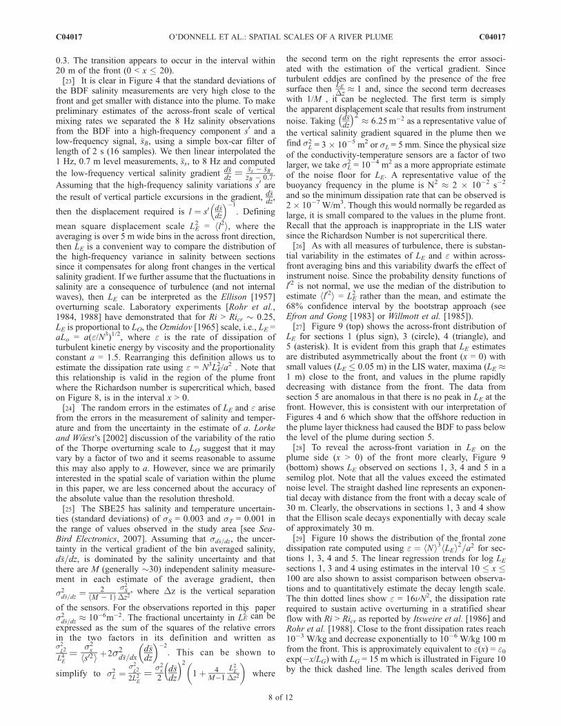
LE for sections 1 (plus sign), 3 (circle), 4 (triangle), and5 (asterisk). It is evident from this graph that LE estimatesare distributed asymmetrically about the front (x = 0) withsmall values (LE � 0.05 m) in the LIS water, maxima (LE �1 m) close to the front, and values in the plume rapidlydecreasing with distance from the front. The data fromsection 5 are anomalous in that there is no peak in LE at thefront. However, this is consistent with our interpretation ofFigures 4 and 6 which show that the offshore reduction inthe plume layer thickness had caused the BDF to pass belowthe level of the plume during section 5.[28] To reveal the across-front variation in LE on the

plume side (x > 0) of the front more clearly, Figure 9(bottom) shows LE observed on sections 1, 3, 4 and 5 in asemilog plot. Note that all the values exceed the estimatednoise level. The straight dashed line represents an exponen-tial decay with distance from the front with a decay scale of30 m. Clearly, the observations in sections 1, 3 and 4 showthat the Ellison scale decays exponentially with decay scaleof approximately 30 m.[29] Figure 10 shows the distribution of the frontal zone

dissipation rate computed using e ¼ hNi3hLEi2=a2 for sec-tions 1, 3, 4 and 5. The linear regression trends for log LEsections 1, 3 and 4 using estimates in the interval 10 � x �100 are also shown to assist comparison between observa-tions and to quantitatively estimate the decay length scale.The thin dotted lines show e = 16nN2, the dissipation raterequired to sustain active overturning in a stratified shearflow with Ri > Ricr as reported by Itsweire et al. [1986] andRohr et al. [1988]. Close to the front dissipation rates reach10�3 W/kg and decrease exponentially to 10�6 W/kg 100 mfrom the front. This is approximately equivalent to e(x) = e0exp(�x/LG) with LG = 15 m which is illustrated in Figure 10by the thick dashed line. The length scales derived from

C04017 O’DONNELL ET AL.: SPATIAL SCALES OF A RIVER PLUME

8 of 12

C04017

regression through the data obtained on each section arelisted in Table 2 and the trends are shown by the solid linesin Figure 10. Though dissipation rate estimates suggest thatthe maximum decreases with distance from the source andthat LG increases, these differences are not statisticallysignificant and additional observations are required toaddress these issues.[30] Though the measurements by the REMUS AUV

were acquired more than an hour after the ship measure-ments and, as is clear in Figure 3, approximately 300 mwest of the frontal crossing on section 3, they provide anindependent and more precise estimate of the dissipationrate distribution. Figure 11 displays the dissipation rateestimate assuming isotropy at viscous dissipation scales.These were computed from micro-scale velocity gradientsmeasured by the shear probes following the processingapproach detailed by Goodman et al. [2006] and averagedin 10 m across-front bins. A maximum value of e = 7 �10�5 W kg�1 occurs near the front and e decreases withdistance from the front. The maxima is somewhat lowerthan those shown in Figure 10 (though it is still very large).This difference is partially due to the larger spatial averag-ing window employed. However, the across-front decay rateis entirely consistent with the ship-based measurements.This is demonstrated by comparison of the measurements in

Figure 11 with the straight dashed line which shows ane(x) / exp (�x/LG) with a length scale LG = 15 m.

5. Summary and Discussion

[31] Though river plumes like that of the Connecticuthave been reported in many locations [e.g., Wright andColeman, 1971; Stronach, 1977; Ingram, 1981; Freeman,1982; Lewis, 1984; Luketina and Imberger, 1987; Geyer etal., 1998; Hickey et al., 1998] there have been few system-atic observations of the along front variation of the plumecharacteristics. We believe this report is the first quasi-synoptic, high-resolution view of the along-front variationin plume layer thickness and salinity. We find that the plumelayer at the front thins in the offshore direction while thesalinity increases. At 1 km from the source, the across-frontsalinity jump is half of that at the source. This behavior islargely consistent with the predictions of the models ofGarvine [1982] and O’Donnell [1988, 1990]. The mecha-nisms that control the relative importance of the verticalexchange with the deeper water and the horizontal exchangewith the plume to the rate of the reduction of the along-frontfreshwater flux remain unresolved. With the data availablewe are unable to adequately resolve the terms in the saltbudget in the frontal zone. An observation campaign withmore vertical resolution of the salinity field together with

Figure 9. (top) The across-front distribution of the square root of the squared Ellison scale, LE,averaged in 5-m across-front bins. Sections 1, 3, 4, and 5 are represented using the same symbols asFigure 8. (bottom) To reveal the across-front and along-front variation of salinity fluctuations thedependence of LE on the across-front distance from the front is shown on a logarithmic axis. The thicksolid line illustrates an exponential decay with a decay length scale of 30 m.

C04017 O’DONNELL ET AL.: SPATIAL SCALES OF A RIVER PLUME

9 of 12

C04017

ADCP data that resolves the near surface advection fluxtoward the front is required.[32] Establishing the mechanisms that control the width

of river plume fronts is likely to be critical to the accurateprediction of the dispersion of terrestrial effluent in thecoastal ocean since a significant amount of mixing occurs inits vicinity. A scale estimate can be developed by consid-eration of a simple conceptual gravity current model andlaboratory experiments. There is considerable literature inwhich this approach has been used to model the spreadingof buoyant fluids and much of it is coherently summarizedat an introductory level by Simpson [1987]. The analyticwork of Benjamin [1968] was extended in a semi-empiricalanalysis and a series of laboratory experiments by Britterand Simpson [1978] and Simpson and Britter [1979] tomodel the spreading of negatively buoyant fluids. Subse-quently, Simpson and Nunes [1981] and Garvine [1981]based their interpretation of the dynamics of a small-scaleriver plume fronts on this literature. Underlying thesemodels is the idea that the Kelvin-Helmholtz instabilitiesat the leading edge of the gravity current lead to thegeneration of three-dimensional turbulence in the stratifiedshear layer between the buoyant and ambient fluids. In both

the analysis of Britter and Simpson [1978] and the model ofGarvine [1974] the magnitude and spatial rate of decay ofmixing between the layers is prescribed in order to matchobserved density field structure. Our observations that themagnitude of e and, by extension, the vertical eddy diffu-sivity, decays across the frontal zone confirm that theirassumptions were well founded.[33] Rohr et al. [1988] and Itsweire et al. [1993] per-

formed careful and extensive lab experiments on the growthand decay of grid generated turbulence in stratified shearflows. One of the important results was the demonstrationthat in experiments with gradient Richardson number, Ri >Ricr = 0.25, turbulence and vertical mixing was suppressed.Further, for values of the dissipation rate, e < 16vN2, whereN is the buoyancy frequency and v is the molecularviscosity, the vertical turbulent buoyancy flux was effec-

Table 2. Estimates for the Width of the Zone of Active Mixing

Section

1 3 4 5 Mean

LG (m) 11.4 16.7 22.6 16.9LI (m) 23.5 26.7 38.6 26.9 28.9

Figure 10. Across-front distribution of the turbulent kinetic energy dissipation rate for sections 1, 3, 4,and 5. The symbol code is the same as used in Figure 8. The thick solid lines illustrate the best-fitexponential decay of the dissipation rate in the across-front direction for sections 1, 3, and 4. The dottedlines show the Rohr et al. [1988] estimate of the level of dissipation at which mixing ceases.

C04017 O’DONNELL ET AL.: SPATIAL SCALES OF A RIVER PLUME

10 of 12

C04017

tively zero. In experiments with a mean flow in the shearlayer, U, and Ri > Ricr, Itsweire et al. [1993] concluded thatthe vertical buoyancy flux went to zero within 5 buoyancyperiods of passing through the grid, or equivalently after adistance LI = 5U/N from the generation location.[34] If we accept that lab and field observations of the

decay of turbulence should be in agreement once the effectsof stratification begin to dominate and then assume, on thebasis of the flow visualizations of gravity currents ofSimpson and Britter [1979], that any coherent structuresat the leading edge of the front break up into turbulencewithin a few buoyant layer depths from the leading edge,then the scale LI should provide a guide to the width of theactive mixing zone in plume fronts with Ri > Ricr. Note,however, that the flow field in the Connecticut River is not atwo dimensional flow. There is a significant along-frontvelocity component that has shear in both the horizontal andvertical directions. Visual observations (see photograph inFigure 2) and the analysis of ADCP observations in thesame area by Trump and Marmorino [2002, 2003] stronglysuggest that coherent vortices with vertical vorticity com-ponents of magnitude �0.1 s�1 are present at the frontalboundary. Such structures likely enhance the production ofturbulent kinetic energy and modify the distribution of thedissipation rate even where stratification dominates.[35] Computed values for LI using the data from Con-

necticut River plume sections in which N can be estimated(1, 3, 4, and 5) are presented in Table 2. Estimated LI areapproximately 1.5–2 times larger than LG, the decay scalefor e and shown in Figure 10. Since the vertical gradientswere only minimally resolved by our measurements theestimates of LE

2 and N2 are likely to be underestimated.Despite the weakness of the instrumentation, it is clear thatthe spatial decay scale, LG, is the same order of magnitudeas LI and, therefore, we conclude that LI should provide auseful guide for the scale of river plume fronts.[36] An analysis of the frontal zone mechanical energy

budget would be a useful check on the magnitudes of thedissipation rates we estimate but, unfortunately, the nearsurface flow toward the front is unresolved causing the

budget to be too uncertain to provide a constraint on thedissipation rate. Only two previous observational programsin similar environments have been reported with which wecan compare our estimates. Note that the spatial resolutionof those was significantly less than our measurements.Luketina and Imberger [1989] made the first estimatesusing a moored profiler and found a maximum value of10�6 W/kg near a thermal plume front. More recently Ortonand Jay [2005] presented estimates of the variation of ewith distance from the Columbia River plume front usingThorpe sorting [see Thorpe, 1977; Galbraith and Kelley,1996] of measurements by an undulating towed CTD. Theyreported that e varied from 10�3 W/kg at 100 m from thefront to 10�6 W/kg at 1000 m. This is equivalent to a spatialdecay scale of 130 m. Using the reported frontal propaga-tion speed uf = 0.60 m/s as the mean velocity in the shearlayer and a buoyancy frequency value N = 0.05 based on thesalinity distribution, we obtain the estimate LI = 5uf /N =60 m for the scale of the frontal zone width. Again, this isapproximately a factor of 2 less than the observed spatialdecay rate but the correct order of magnitude.[37] Though more detailed measurements of both the

velocity field and density gradients need to be obtained tofurther evaluate the approach to estimating dissipation rate,and more consideration needs to be given to the role of theshear in the along front velocity gradients, the scaleestimate for the width of the region of active mixingpresented here can provide guidance to both observationcampaigns and numerical model formulations to determinethe scale of variations that need to be resolved in studies ofriver plumes.

[38] Acknowledgments. This work was supported by the NationalScience Foundation through grant 0096551 and by the University ofConnecticut. We thank the reviewers of the manuscript and acknowledgethat their criticism led to a clearer presentation of our work. J. O’Donnell isalso grateful to the faculty and staff of the School of Ocean Sciences,University of Wales, Bangor, and the people of Ynys Mon for their adviceand hospitality during the drafting of this manuscript.

ReferencesBenjamin, T. B. (1968), Gravity currents and related phenomena, J. Fluid.Mech., 31, 209–248.

Britter, R. E., and J. E. Simpson (1978), Experiments on the dynamics of agravity current head, J. Fluid. Mech., 88, 223–240.

Deines, K. L. (1999), Backscatter estimation using broadband acousticDoppler current profilers, in Proceedings of IEEE Sixth WorkingConference on Current Measurement, edited by S. P. Andersonet al., pp. 249–253, Inst. of Electr. and Electron. Eng., New York.

Efron, B., and G. Gong (1983), A leisurely look at the bootstrap, the jack-knife, and cross-validation, Am. Stat., 37(1), 36–48.

Ellison, T. H. (1957), Turbulent transport of heat and momentum from aninfinite rough plane, J. Fluid Mech., 2, 456–466.

Freeman, N. G. S. (1982), Measurement and modeling of fresh waterplumes under an ice cover, Ph.D. dissertation, Univ. of Waterloo, Water-loo, Ont., Canada.

Galbraith, P. S., and D. E. Kelley (1996), Identifying overturns in CTDprofiles, J. Atmos. Oceanic Technol., 13, 688–702.

Garvine, R. W. (1974), Dynamics of small-scale fronts, J. Phys. Oceanogr.,4, 557–569.

Garvine, R. W. (1981), Frontal jump conditions for models of shallow,buoyant surface layer dynamics, Tellus, 33, 301–312.

Garvine, R. W. (1982), A steady state model for buoyant surface plumes incoastal waters, Tellus, 34, 293–306.

Garvine, R. W., and J. D. Monk (1974), Frontal structure of a river plume,J. Geophys. Res., 79, 2251–2259.

Geyer, W. R., D. J. Mondeel, P. S. Hill, and T. G. Milligan (1998), The EelRiver Plume during the 1997 flood: Freshwater and sediment transport,Eos Trans. AGU, 79(45), Fall Meet Suppl., F455.

Figure 11. Across-front distribution of the turbulentkinetic energy dissipation rate computed from the shearprobe measurements by the REMUS AUV.

C04017 O’DONNELL ET AL.: SPATIAL SCALES OF A RIVER PLUME

11 of 12

C04017

Goodman, L., E. R. Levine, and R. Lueck (2006), On measuring the termsof the turbulent kinetic energy budget from an AUV, J. Atmos. OceanicTechnol., 23, 977–990.

Hickey, B. M., L. J. Pietrafesa, D. A. Jay, and W. C. Boicourt (1998), TheColumbia river plume study, subtidal variability in the velocity and sali-nity fields, J. Geophys. Res., 103, 10,339–10,368.

Ingram, G. (1981), Characteristics of the Great Whale River plume,J. Geophys. Res., 86, 2017–2023.

Itsweire, E. C., K. Helland, and C. van Atta (1986), The evolution of grid-generated turbulence in a stably-stratified fluid, J. Fluid Mech., 162,299–338.

Itsweire, E. C., J. Koseff, D. A. Briggs, and J. H. Ferziger (1993), Turbu-lence in stratified shear flows: Implications for interpreting shear-inducedmixing in the ocean, J. Phys. Oceanogr., 23, 1508–1522.

Levine, E. R., and R. G. Lueck (1999), Turbulence measurements withan autonomous underwater vehicle, J. Atmos. Oceanic Technol., 16,1533–1544.

Levine, E. R., L. Goodman, and J. O’Donnell (2008), Turbulence in coastalfronts near the mouths of Block Island and Long Island Sounds, J. Mar.Syst., in press.

Lewis, R. E. (1984), Circulation and mixing in estuary outflows, Cont.Shelf Res., 3, 201–214.

Lorke, A., and A. W}uest (2002), Probability density of displacement andoverturning length scales under diverse stratification, J. Geophys. Res.,107(C12), 3214, doi:10.1029/2001JC001154.

Luketina, D. A., and J. Imberger (1987), Characteristics of a surfacebuoyant jet, J. Geophys. Res., 92, 5435–5447.

Luketina, D. A., and J. Imberger (1989), Turbulence and entrainment in abuoyant surface plume, J. Geophys. Res., 94, 12,619–12,636.

O’Donnell, J. (1988), A numerical technique to incorporate frontalboundaries in layer models of ocean dynamics, J. Phys. Oceanogr.,18, 1584–1600.

O’Donnell, J. (1990), The formation and fate of a river plume: A numericalmodel, J. Phys. Oceanogr., 20, 551–569.

O’Donnell, J. (1993), Surface fronts in estuaries: A review, Estuaries,16(1), 12–39.

O’Donnell, J. (1997), Observations of near surface currents and hydrogra-phy in the Connecticut River plume with the SCUD array, J. Geophys.Res., 102, 25,021–25,033.

O’Donnell, J., G. O. Marmorino, and C. L. Trump (1998), Convergence anddownwelling at a river plume front, J. Phys. Oceanogr., 28, 1481–1495.

Orton, P. M., and D. A. Jay (2005), Observations at the tidal plume front of ahigh-volume river outflow, Geophys. Res. Lett., 32, L11605, doi:10.1029/2005GL022372.

Osborn, T. R., and W. R. Crawford (1982), An airfoil probe for measur-ing turbulent velocity fluctuations in water, in Air-Sea Interactions,Instruments andMethods, edited by F. Dobson, L. Hasse, and R. Davis,pp. 369–386, Plenum, New York.

Ozmidov, R. V. (1965), On the turbulent exchange in a stably stratified ocean,Izv. Acad. Sci. USSR Atmos. Ocean. Phys., Engl. Transl., 1, 853–860.

RD Instruments (1997), DR/SC Acoustic Doppler current profiler technicalmanual, P/N 951-6046-00, San Diego Calif.

Rohr, J. J., E. C. Itsweire, K. N. Helland, and C. W. Van Atta (1984),Mixing efficiency in stably stratified decaying turbulence, Geophys.Astrophys. Fluid Dyn., 29, 221–236.

Rohr, J. J., E. C. Itsweire, K. N. Helland, and C. W. Van Atta (1988),Growth and decay of turbulence in a stably stratified shear flow, J. FluidMech., 195, 77–111.

Sea-Bird Electronics (2007), SBE 25 Sealogger CTD Users Manual(Version 015), Sea-Bird Electron., Inc., Bellevue, Wash.

Seim, H. E. (1999), Acoustic backscatter from salinity microstructure,J. Atmos. Oceanic Technol., 16, 1991–1998.

Simpson, J. E. (1987), Gravity Currents in the Environment and Labora-tory, John Wiley, Hoboken, N. J.

Simpson, J. E., and R. E. Britter (1979), The dynamics of the head of agravity current advancing over a horizontal surface, J. Fluid Mech., 94,477–495.

Simpson, J. H., and R. A. Nunes (1981), The tidal intrusion front: Anestuarine convergence zone, Estuarine Coastal Shelf Sci., 13, 257–266.

Smyth, W. D., and J. N. Moum (2000), Length scales of turbulence instably stratified mixing layers, Phys. Fluids, 12, 1327–1342.

Stronach, J. A. (1977), Observations andmodeling studies of the Frazer Riverplume, Ph.D. dissertation, Univ. of B. C., Vancouver, B. C., Canada.

Thorpe, S. A. (1977), Turbulence and mixing in a Scottish loch, Philos.Trans. R. Soc., Ser. A, 286, 125–181.

Trump, C. L., and G. O. Marmorino (2002), Spatial processing of range-binADCP data to resolve small-scale frontal features, J. Atmos. OceanicTechnol., 19, 1461–1468.

Trump, C. L., and G. O.Marmorino (2003), Mapping small-scale along-frontstructure using ADCP acoustic backscatter range-bin data, Estuaries,26(4A), 878–884.

von Alt, C., B. Allen, T. Austin, and R. Stokey (1994), Remote environ-mental measuring units, in Autonomous Underwater Vehicle Technology,pp. 13–19, Inst. of Electr. and Electron. Eng., New York.

Willmott, C. J., S. G. Ackleson, R. E. Davis, J. J. Feddema, K. M. Klink,D. R. Legates, J. O’Donnell, and C. M. Rowe (1985), Guidelines for theevaluation and comparison of models, J. Geophys. Res., 90, 8995–9005.

Wright, L. D., and J. M. Coleman (1971), Effluent expansion and mixing inthe presence of a salt wedge. Mississippi River delta, J. Geophys. Res.,76, 8649–8661.

�����������������������S. G. Ackleson, Office of Naval Research, 800 N. Quincy Street,

Arlington, VA 22043, USA.E. R. Levine, Naval Undersea Warfare Center, Code 8211, Newport,

RI 02841, USA.J. O’Donnell, Department of Marine Sciences, University of Connecticut,

Groton, CT 06340, USA. (james.odonnell@uconn.edu)

C04017 O’DONNELL ET AL.: SPATIAL SCALES OF A RIVER PLUME

12 of 12

C04017