Estimation of abl Parameters Using the Vertical Velocity Measurements of an Acoustic Sounder

ESTIMATION OF ABL PARAMETERS USING THE VERTICALVELOCITY MEASUREMENTS OF AN ACOUSTIC SOUNDER

J. A. KALOGIROS1, C. G. HELMIS1, D. N. ASIMAKOPOULOS1,2 and P. G.PAPAGEORGAS1

1Department of Applied Physics, University of Athens, Greece2Institute of Meteorology and Physics of the Atmospheric Environment, National Observatory of

Athens, Greece

(Received in final form 13 October 1998)

Abstract. The friction velocity, the surface heat flux and the height of the Atmospheric Bound-ary Layer (ABL) are important parameters. In this work, vertical velocity variance (σ2

w) and windvelocity structure parameter (C2

v ) profiles estimated by acoustic sounder measurements are used,along with similarity relations, to estimate these parameters in the unstable Atmospheric BoundaryLayer and the friction velocity in the stable one. The data were collected by two acoustic sounderswith different height range and resolution under various atmospheric conditions (stability) and attwo experimental sites in different terrain. TheC2

v profiles are estimated using gate difference of thevertical velocity measurements and the assumption of local isotropy. The vertical velocity data arecorrected for the significant effects of noisy measurements and sampling volume averaging on theσ2w andC2

v estimations using original techniques that are presented in this work. The results of thesimilarity method using acoustic sounder data are compared against estimates of the correspondingatmospheric parameters obtained from direct measurements. The comparison confirms the ability ofthe method to provide reasonably accurate estimates of these parameters especially in the middle ofthe day.

Keywords: Acoustic sounder, Vertical velocity, Noise reduction, Volume averaging correction, Sur-face turbulent fluxes, CBL height.

1. Introduction

Knowledge of the value of the turbulent surface heat (Q0 = w′θ ′0, where theoverbar and the prime indicate run time average and deviation from the mean

value, respectively) and momentum (−u2∗ = −(u′w′2 + v′w′2)1/20 , whereu∗ isthe friction velocity) fluxes and the height of the first temperature inversion (Zi)at the top of the Convective Boundary layer (CBL) is significant for the predictionof the boundary layer evolution and its diffusion capabilities. Various methods todetermine these parameters could be used, including one point (in-situ) or remotemeasurements. Remote sensing techniques are representative of a large volumeof the atmosphere. This spatial average of atmospheric parameters is often moreappropriate than single point measurements in studies of the ABL (for example,energy balances over a large area). This work considers methods to estimate these

Boundary-Layer Meteorology91: 413–449, 1999.© 1999Kluwer Academic Publishers. Printed in the Netherlands.

414 J. A. KALOGIROS ET AL.

parameters using a monostatic acoustic sounder and, specifically, vertical velocitymeasurements at various heights.

The profile of the vertical velocity variance (σ 2w) calculated with an acoustic

sounder and its similarity form in the CBL have been used from many workers inthe field in order to provide estimates ofQ0, u∗ andZi (Weill et al., 1980; Taconetand Weill, 1982; Greenhut and Mastrantonio, 1989; Keder et al., 1989; Kalogiroset al., 1994; Helmis et al., 1994, 1995). The results showed significant precisionfor theu∗ estimates but limited precision for theQ0 andZi estimates. The analysisof the profile of the velocity structure parameter (C2

v ) is, also, a method that canprovide accurate estimates ofQ0. This method has only been tested indirectly in afew case studies with sodar data (Gaynor, 1977; Melling and List, 1980). However,it has not been proposed or tested as a method for the estimation ofQ0 sinceaccurate estimates ofC2

v with acoustic sounders are difficult. The large samplingperiod, the large distance between gates of measurement that usually falls outsidethe inertial subrange, the noise in velocity measurements and the sampling volumeaveraging may significantly affect the accuracy of the measurements.

In this paper, an integrated similarity method of analysis ofσ 2w andC2

v profilesestimated by an acoustic sounder is presented. The method includes the generallocal isotropy form of the structure function of the vertical velocity of wind, the re-duction of noise in the vertical velocity measurements of the acoustic sounder usinga continuity and a local isotropy check and the combined correction ofσ 2

w andC2v

profiles for the effect of sampling volume averaging instead of arbitrary correctionmethods against in-situ measurements at a selected height (Keder et al., 1989). Theresults of the method applied to large data sets collected with different acousticsounder systems under various atmospheric conditions (stability) and at differentterrain are compared to estimates ofQ0, u∗ andZi from direct measurements.

2. Experimental Layout

The data used in this paper were collected during the summer of 1993 in the centreof the urban area of Athens on the top of the hill of National Observatory of Athens(NOA, 110 m ASL) and during the summer of 1995 at the flat, rural area (50 m ASLwith sparse trees) of Messogia Plain (Spata) in Attika peninsula, Greece (Figure 1).The hill of NOA is characterised by a gently rising topography (about 10◦ slope)with scattered pine trees. It is surrounded by a densely-built urban area. The ver-tically oriented, monostatic acoustic sounders used at the NOA experimental sitewere a combination of a low range-high resolution one (4.3 kHz) designed at theAthens University, (Asimakopoulos et al., 1987), with a high range one (1.6 kHz).A system similar to the latter one was used at the Messogia Plain. Table I showsthe operating parameters of the acoustic sounders. The average vertical velocity ofthe wind in the gate volume was estimated from the Doppler frequency shift of thebackscattered signal using an FFT analysis.

VERTICAL VELOCITY MEASUREMENTS OF AN ACOUSTIC SOUNDER 415

Figure 1.The greater Athens area and the experimental sites NOA and Spata indicated with bullets(height contours of 200 m).

A 12 m high meteorological mast equipped with a UVW propeller anemometer(NEZII, Alcyon S.A.) and a fast responding temperature platinum wire (12.5µmdiameter and about 20 Hz frequency response) sensor was established close to theacoustic sounders at both sites. The sampling rate of these sensors was 1 Hz andthey provided a direct method (eddy correlation) for estimating the surface heatand momentum fluxes. The accuracy of turbulent fluxes estimates using a propelleranemometer is discussed in Section 4.1.

The time duration of the analysis runs for the sodar and the mast data was 30 minfor the data collected at Messogia Plain and 45 min for the data collected at NOA(because of the slower repetition rate of the high range 1.6 kHz acoustic sounder atthat site) in order to obtain good statistical precision and almost static atmosphericconditions.


TABLE I

Operating parameters of the acoustic sounders. The pulse repetition rate inside thebrackets corresponds to the 1.6 kHz system operating at the NOA site.

Operating parameter High range system High resolution system

Transmit frequency (kHz) 1.6 4.3

Pulse length (msec) 108 54

Pulse repetition period (sec) 5.00 (10.90) 5.45

Maximum range (m) 800 400

Minimum discernible height (m) 60 13

Gate length (m) 34.5 17.2

Acoustic antenna 1.2 m parabolic disc 5× 5 tweeters array

3. Data Processing and Methods of Analysis

3.1. CALCULATION OF THE WIND VELOCITY STRUCTURE PARAMETER

A usual method to estimateC2v by wind velocity measurements is the structure

function of one its components. This method uses the measurements at two pointsin space (or in time, using Taylor hypothesis). Under local isotropy conditions andfor separation distances inside the inertial subrange, this function follows the 2/3power law. However, in the case of acoustic sounders the distance between thewind velocity measurements is, usually, outside the inertial subrange (especially atlow heights of measurement or under stable atmospheric conditions) and, thus, amore general formula for the structure function is needed.

Under the assumption of local isotropy, the structure function of the verticalvelocity for a vertical distance1z (the distance between the middle of the gates) isgiven by the following relation (Tatarskii, 1971):

Dw(1z) = (w′(z+1z)− w′(z))2

= 2σ 2w

[1− 22/3

0(1/3)

(1z

2Lw

)1/3

K1/3

(1z

2Lw

)], (1)

whereσ 2w is the average of the variances at each gate,Lw is the integral scale of

the vertical velocity field,0(x) is the Gamma function andK1/3(x) is the modi-fied Bessel function of the second kind and 1/3 order. The overbar indicates timeaverage and the prime indicates deviation from the mean value. The varianceσ 2

w

is really the average of the values at the two measurement points. We approxim-


ated Equation (1) using its asymptotic behaviour and exponential functions (seeAppendix A) by:

Dw(1z) ≈ 2σ 2w

{Gx2/3 exp(−x/4), x ≤ 1.5

1− Px−1/6 exp(−x), x > 1.5,(2)

wherex =1z/(2Lw),G= [0(2/3)/0(4/3)](1/2)2/3 andP = 22/3√π/2/0(1/3).Equations (1) and (2) hold for any distance1z larger than the inner scale of turbu-lence (a few mm), even for distances larger thanLw, provided that local isotropyholds (i.e., the statistical parameters of the wind field do not change significantlywith direction). The velocity structure functionC2

v is estimated directly from thestructure function when1z is in the inertial subrange(1z < Lw):

Dw(1z) = C2v (1z)

2/3. (3)

In the case that1z is not much larger thanLw, Equation (1) is similar to Equation(3) with the addition proportionality factor of 0.7–0.9 in the right hand side of(3). Also, Equations (1) and (2) are more accurate than Equation (3) in the inertialsubrange when1z is not much smaller thanLw and, thus, it is preferable to usethem in every case. The application of the 2/3 power law underestimatesC2

v by10–30% for1z = 0.5− 1.5Lw.

Using Equation (1) for1z � Lw and (3) and retaining the first two terms inthe series expansion ofK1/3(x) (see Equation (A.1) in Appendix A) the structureparameter is given by (Tatarskii, 1971):

C2v =

2σ 2w0(2/3)

(4Lw)2/30(4/3). (4)

Thus, in generalC2v is calculated for any distance1z between the measurement

gates if the values ofσ 2w andLw are known. The value ofLw is estimated from

Equation (2) using a converging iterative procedure whereσ 2w andDw(1z) have

the values measured by the acoustic sounder. In this scheme, the corrections ofσ 2w

andDw(1z) by the local isotropy check and for the sampling volume averaging,which are described in Section 3.2, are also included.

It should be noticed that the spectral content ofDw(1z) is dominated by lowwavenumberskx in the mean wind direction (see Equation (8) in Section 3.2.2).This is easily understood from the fact that the one-dimensional spectrum of1w/1z in the vertical direction has the well knownk1/3

z dependence. But, theprojection of a wavenumberkz, propagating nearly in the vertical direction wherethe fall off of energy due to the separation1z starts, appears on the streamwise axisto be a very low wavenumberkx (Lumley and Panofsky, 1964). The wavenumberkxis related to frequency with Taylor’s hypothesis. Thus, the relatively low samplingfrequency of the acoustic sounder systems (a few seconds) is usually adequate for


the estimation ofDw(1z), but, probably, not for the estimation ofDw(1x) (charac-terised by ank1/3

x dependence of its one-dimensional spectrum) on the streamwiseaxis using Taylor’s hypothesis.

3.2. VERTICAL VELOCITY DATA PROCESSING

There are several factors that introduce errors in the estimation of the averageradial wind velocity in a measurement gate of an acoustic sounder (Brown, 1974;Kristensen and Gaynor, 1986). These errors include refraction of the acoustic beam(Georges and Clifford, 1972; Spizzichino, 1974), beam wander and tilt (Cliffordand Brown, 1980; Neff, 1978), spectral broadening of the backscattered signal(Tatarskii, 1971; Brown and Clifford, 1973; Brown, 1974) and the introductionof the transverse wind velocity component or the non uniform distribution of tur-bulence within the beam volume (Spizzichino, 1974). Under low horizontal wind(less than 10 m s−1) and for a well designed system, these factors are not sosignificant as the effect of the environmental or system noise (Spizzichino, 1974)for the estimation of the vertical velocity. A check of the velocity time series fornoisy measurements is always necessary, otherwise there is an increase of fluctu-ation energy due to the noise effect. On the other hand, the calculation of secondmoments (variance and structure function) of velocity using the average velocityvalues in the gate volume leads to a loss of energy despite the frequency aliasedenergy, since this procedure is equivalent to a low-pass filtering (Kristensen andGaynor, 1986; Finkelstein et al., 1986b; Chintawongvanich et al., 1989). In thenext two paragraphs, the techniques that we developed and used in this work forthe reduction of noise and the volume averaging correction are described.

3.2.1. Noise ReductionAn initial criterion for the acceptation of a velocity measurement is the signal tonoise ratio, which is estimated from the degree of spread of the frequency spec-trum of the backscattered signal in the corresponding gate (Papageorgas et al.,1993). A lower acceptation limit of 0.75 for the signal to (signal + noise) ratiowas used in this study. The measurements initially characterised as good ones arethen used to calculate the median value (instead of the average one to avoid anybias) of the linear interpolations among the neighbour measurements around thecurrently examined point in the velocity time series. The neighbour measurementsare considered in the time-height grid.

An upper threshold of 0.5 m s−1 for the difference between the measurementvalue and the median one was used to accept or else to replace the measurement bythe median value. This method is really a continuity (or consistency) check of thevelocity field (Weber et al., 1993). The replacement of noisy measurements by themedian values instead of a simple rejection increases the number of measurementsused and, thus, the accuracy of the statistical calculations. Only time series with


less than 30% corrected data points were allowed to take part in the calculation ofvelocity moments.

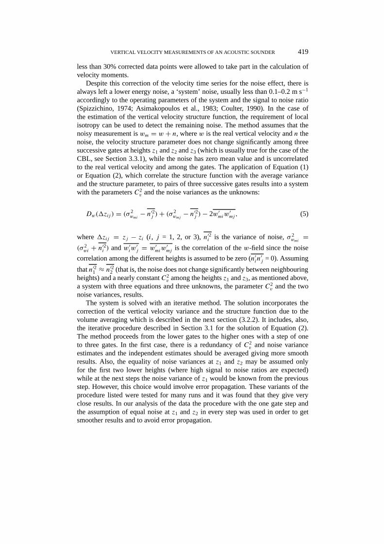
Despite this correction of the velocity time series for the noise effect, there isalways left a lower energy noise, a ‘system’ noise, usually less than 0.1–0.2 m s−1

accordingly to the operating parameters of the system and the signal to noise ratio(Spizzichino, 1974; Asimakopoulos et al., 1983; Coulter, 1990). In the case ofthe estimation of the vertical velocity structure function, the requirement of localisotropy can be used to detect the remaining noise. The method assumes that thenoisy measurement iswm = w + n, wherew is the real vertical velocity andn thenoise, the velocity structure parameter does not change significantly among threesuccessive gates at heightsz1 andz2 andz3 (which is usually true for the case of theCBL, see Section 3.3.1), while the noise has zero mean value and is uncorrelatedto the real vertical velocity and among the gates. The application of Equation (1)or Equation (2), which correlate the structure function with the average varianceand the structure parameter, to pairs of three successive gates results into a systemwith the parametersC2

v and the noise variances as the unknowns:

Dw(1zij ) = (σ 2wmi− n′2j )+ (σ 2

wmj− n′2j )− 2w′miw

′mj , (5)

where1zij = zj − zi (i, j = 1, 2, or 3),n′2i is the variance of noise,σ 2wmi=

(σ 2wi + n′2i ) andw′iw

′j = w′miw

′mj is the correlation of thew-field since the noise

correlation among the different heights is assumed to be zero (n′in′j = 0). Assuming

thatn′21 ≈ n′22 (that is, the noise does not change significantly between neighbouringheights) and a nearly constantC2

v among the heightsz1 andz3, as mentioned above,a system with three equations and three unknowns, the parameterC2

v and the twonoise variances, results.

The system is solved with an iterative method. The solution incorporates thecorrection of the vertical velocity variance and the structure function due to thevolume averaging which is described in the next section (3.2.2). It includes, also,the iterative procedure described in Section 3.1 for the solution of Equation (2).The method proceeds from the lower gates to the higher ones with a step of oneto three gates. In the first case, there is a redundancy ofC2

v and noise varianceestimates and the independent estimates should be averaged giving more smoothresults. Also, the equality of noise variances atz1 and z2 may be assumed onlyfor the first two lower heights (where high signal to noise ratios are expected)while at the next steps the noise variance ofz1 would be known from the previousstep. However, this choice would involve error propagation. These variants of theprocedure listed were tested for many runs and it was found that they give veryclose results. In our analysis of the data the procedure with the one gate step andthe assumption of equal noise atz1 andz2 in every step was used in order to getsmoother results and to avoid error propagation.


Figure 2.An application of noise detection using the local isotropy check after the continuity checkof the vertical velocity measurements (for the run 1017–1047 LST on 4/9/95 at Messogia site usingthe 1.6 kHz acoustic sounder).

An example of the application of this technique after the continuity check ispresented in Figure 2. The noise level is low (the continuity check has been applied)and increases with height (i.e., inversely to the signal to noise ratio), as it is usuallyexpected. However, the subtraction of this noise may be significant, especially atthe higher heights, because the volume averaging correction applied after the noisereduction step would exaggerate it. The negative values at the lower heights meanthat the continuity check subtracted too much energy from these vertical velocitytime series and would be missed if it was assumed that the lower measurement gatecharacterised by high signal to noise ratio is noise free. Also, the local isotropycheck can be considered as a quality test of the measurements after the continuitycheck: if the detected noise is high (for example, higher than the threshold used inthe continuity check) the measurements should be rejected.

3.2.2. Volume Averaging CorrectionThe spectrum of the backscattered signal in every gate is composed from thecontribution of the various turbulent elements in the sampling volume. Thus, theaverage frequency Doppler shift corresponds to the average radial velocity in thesampling volume formed by the gate length and the acoustic beam. In the case of


the calculation of the vertical velocity variance, the relation between the measuredvolume averaged varianceσ 2

wmand the true oneσ 2

w is (Kristensen and Gaynor,1986):

σ 2wm/σ 2

w = 1− 1.214f (1z/1h)(0.30031h/Lw)2/3, (6)

where1z is the gate length and1h is the horizontal diameter of the acoustic beam(assumed to lie in the inertial subrange). We approximated the functionf (x) (seeAppendix A) by:

f (x) = 3

2

∫ 1

0(1− s2)(1− s2 + s2xx)1/3 ds

≈{

0.326(1+ x2)1/3+ 0.59, x ≤ 2

(27/55)x2/3 + 0.918 exp(−0.64√x), x > 2

, (7)

wherex = 1z/1h. This function takes values from 0.92 to 1.15 forx = 0 to 2.In the case of line averaging, the horizontal diameter is removed from (6) takingthe limit1h→ 0. The integral lengthLw may be replaced by the variance and thestructure parameter of the vertical velocity, which are both measured by the acous-tic sounder, according to Equation (4). Thus, there is no need for an approximateestimation ofLw as the one used by Kristensen and Gaynor (1986).

In the case of the structure functionDw(1z), the inclusion of a Gaussian trans-fer functionH(k) = exp{−0.30032[12

zk2z −12

h(k2x + k2

y)]}, wherek = (kx , ky , kz)is the wavenumber vector, similar to the one used by Gaynor (1977) and Kristensenand Gaynor (1986), into the equation of the measured structure functionDwm(1z),according to Tatarskii (1971), gives:

Dwm(1z) = 2∫ ∫ +∞

−∞

∫H(k)[1− cos(kz1z)]

(1− k

2z

k2

)E(k)

4πk2d3k, (8)

whereE(k) is the three-dimensional spectrum of wind velocity, which has a−5/3dependence in the inertial subrange assuming that the one-dimensional spectrumV (k) = 0.125C2

v k−5/3 (Tatarskii, 1971). Extending this law tok = 0, which is

justifiable when the volume dimensions and the separation distance1z lie in theinertial subrange (Kristensen and Gaynor, 1986), and using polar coordinates andnumerical integration of the resulting one-dimensional integral, we approximatedEquation (8) (see Appendix A) by the following relation for the usual case of1z/1z > 0.1:

Dwm(1z) ≈ Dw(1z)(1+ x21)−2/3

×{

1− (1− A0)[1− exp(−A1x2/32 )], 1h > 0

B0, 1h = 0, (9)


whereA0 = B0[1− exp(−0.552x)], B0 = 0.845+ (1− 0.845)exp(−8x1), A1 =1.215 exp(0.355x), x = 1z/1h, x1 = 1z/1z andx2 = 1h/1z = x1/x.Dw(1z)

is assumed to be given by inertial subrange law Equation (3). When1z is largerthanLw, but not too much, Equation (9) is expected to hold approximately sinceEquation (3) has only an additional factor of 0.7–0.9 in the right hand side.

From the equations presented above and Equation (1), it is clear that the correc-tion of one ofσ 2

w or C2v requires the correct value of the other. Thus, a combined

iterative procedure is used which incorporates the volume averaging correction forboth parameters, the general isotropy form of the structure function and the localisotropy check for noise detection, as already described in Section 3.2.1.

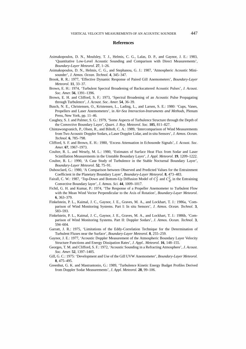
In Figure 3, an application of the volume averaging correction to theσ 2w andC2

v

profiles is shown. The difference of the profiles before and after the correction isclearly significant. The correction includes the removal of noise detected with thelocal isotropy check. It should be mentioned that the ‘measured’ profiles are theones just after the continuity check of the vertical velocity time series for noisymeasurements and, thus, noisy or generally suspicious measurements have beenreplaced by median of neighbours interpolation. However, this implies that theoriginal time series has been smoothed at less than 30% of the points (see Section3.2.1).

3.3. ANALYSIS OF THEσ 2w AND C2

v PROFILES

The profiles ofσ 2w andC2

v measured with acoustic sounders are analysed using thecorresponding similarity relations (Sorbjan, 1988; Stull, 1988; Sorbjan et al., 1991)which have been verified mainly over flat uniform terrain. The analysis aims at theindirect estimation of ABL parameters (the friction velocityu∗, the surface heatflux Q0 and the heightZi of the middle of the first inversion of CBL even whenit is above the range of the acoustic sounder) by these profiles. In the next twoparagraphs, the similarity relations that were used and the method of fit of theserelations to the measured profiles are presented.

3.3.1. Similarity RelationsThe similarity relation used for the analysis of theσ 2

w profile in the CBL is acombination of the surface-layer relation (Kaimal et al., 1976; Weill et al., 1986)and the mixed-layer one (Lenschow et al., 1980):

σ 3w = (1.25)3[u3

∗ + C(kg/2)Q0z][1− 1+ ae

1+ 2ae(z/Zi)

]3

, (10)

wherez is the height above ground,k = 0.35 is the von Karman constant,g isthe acceleration of gravity,2 is the average potential temperature andae is theentrainment coefficient. The constantC shows the relative importance of thermalto mechanical production of turbulence and it takes a value of 3.43 over flat terrain.According to Rotach (1993) mechanical production dominates the thermal one in


urban sites (like the NOA site) and a modified value of 2.00 may be used. Theentrainment coefficient for a well developed CBL has a value of about 0.2 (then theproportionality factor ofz/Zi gets the usual value of about 0.8). Thus, Equation(10) presents a characteristic maximum around 0.3–0.4Zi in the well developedCBL. A more general formula, which includes the contribution of surface mo-mentum flux in addition to heat flux, may be used according to Dubosclard (1980)and Fairall (1987):

ae = 0.2[1+ 2.8(−L/Zi)], (11)

whereL = −u3∗/(kgQ0/2) is the Obukhov length. The inclusion of the propor-tionality factor with the entrainment coefficient in Equation (10) ensures thatσwgoes to zero (no turbulence) at the top of the inversion (i.e., in the free atmosphere).This height is defined as the point aboveZi where the heat flux, which varies almostlinearly with height, becomes zero.

In the stable ABL, mechanical production dominates andσw is nearly constantin the surface layer (i.e., at the lower heights of measurement by the acousticsounders) and then decreases with height until reaching zero at the top of ABL(Stull, 1988). Thus, in the case of the stable ABL only an estimation of frictionvelocity usingσw measurements is possible. The actual range of acoustic soundermeasurements of vertical velocity is limited by the depth of the stable ABL sinceturbulence is greatly reduced above it (low signal to noise ratio). Our measuredσwprofiles within the stable ABL did not show any systematic trend with height andits average value was assumed to be equal to the similarity surface value of 1.25u∗(Weill et al., 1986).

The structure parameterC2v is connected to the dissipation rate (ε) of the turbu-

lent kinetic energy with the relationC2v = 2ε2/3 (Tatarskii, 1971; Kaimal, 1973).

The similarity prediction for the dissipation rateε in the surface layer is (Wyngaardand Cote, 1971):

ε =

u3∗kz(1+ 0.75|z/L|2/3)3/2, L < 0

u3∗kz(1+ 2.5|z/L|3/5)3/2, L > 0

. (12)

This profile is difficult to fit to acoustic sounder measurements because it requiresvery accurate estimates ofε and, thus, it was not used in our data analysis. Inaddition, the measurement heights should be within the surface layer and this ispossible only with high resolution mini acoustic sounders.

However, in the mixed layer of the unstable atmospheric boundary layer (z �−L) the value ofε is nearly steady with a small negative trend (Kaimal et al.,1976; Gaynor, 1977; Weill et al., 1978; Caughey and Palmer, 1979; Lenschow etal., 1980; Melling and List, 1980):

ε = 0.65(g/2)Q0, (13)


where the proportionality constant has been found to vary around 0.5. This relationis an indication of a degree of balance between the thermal production (redistrib-uted by turbulent vertical transport) and the dissipation of TKE in the mixed layerwhere the mechanical energy production is quite small (less than 20% ofε) due tothe usually near-zero wind shear. Thus, the average value ofC2

v in the mixed layercan easily give an estimate of the surface heat flux.

Finally, when the contribution of humidity fluctuations is significant to thebuoyancy flux(g/θv)w′θ ′v (usually over water surfaces) which enters into the pro-duction of the turbulent kinetic energy, the heat fluxQ0 in the previous relationsshould be replaced by the virtual temperature fluxQv0 = w′θ ′v ≈ Q0(1+ 0.07/B)(Lumley and Panofsky, 1964; Stull, 1988).θv = θ(1 + 0.61r), wherer is thewater vapour mixing ratio, is the virtual potential temperature andB is the surfaceBowen ratio of the sensible to latent heat flux. Thus, the profiles ofσ 2

w andC2v

can give estimates of buoyancy flux which is usually desirable. However, our datawere obtained over land sites where the contribution of humidity fluctuations isestimated to be insignificant (large values of the surface Bowen ratio).

3.3.2. Profile FitsThe profiles ofσ 2

w andC2v measured with the acoustic sounder are fitted with the

similarity relations (10) and (13), respectively. The parameters of the fit areu∗,Q0, Zi in the case ofσ 2

w andQ0 in the case ofC2v . Thus, in the first case the

determination of the subset of parameters which will give the best fit is needed.The possible subsets are (a)u∗, Q0 andZi when the measurements cover most ofthe CBL, (b)Q0 andZi when the lower part of the CBL (and especially the surfacelayer) is not covered by the measurements, (c)u∗ andQ0 when the higher part ofthe CBL (including the local maximum of the profileσ 2

w) is not covered and (d)u∗only when this is not the case of CBL.

The fit of the theoretical relationyt with np parameters to the experimentalprofile y with n data points is achieved minimising the absolute error (robust es-timation) in order to exclude false measurements (outliers) or parts of the profilethat cannot be described by the theoretical relation (for example, the temperatureinversion layer at the top of CBL). After the first fit, the measurements that departedmore than(1+r), wherer = [∑n

1(yt− y)2/∑n

1(y− y)2]1/2 is the correlation coef-ficient, the average standard deviation from the theoretical relation were rejectedand the fit was repeated. The minimisation of the absolute error is achieved withthe downhill simplex method (Press et al., 1986). The significance of the fit isexamined with anF -test on the function

F = (n− np)(np − 1)

r2

(1− r2). (14)

In the case of only one parameter, anχ2-test of the relative square error∑n

1[(yt −y)/yt ]2 with n−1 degrees of freedom is used. The accepted level of significance for


the rejection of the hypothesis of zero correlation or large square error used in thisstudy was relatively high (10%) because of the scatter which is usually observed inthe acoustic sounder measurements.

In the case of theσ 2w profiles, the actual subset of the parameters of the fit was

determined for the choice which gives the smaller value of the function 1/F . Thisfunction is the ratio of the unbiased square error of the fit to the variance of the fitaround the mean value of the profile and presents a minimum for the subset of theparameters of the best fit. When a value ofQ0 was estimated by theσ 2

w profile, un-stable atmospheric conditions were assumed and, thus, Equation (13) for the profileof C2

v in the mixed layer could be used to obtain another estimate ofQ0. A betterindicator of unstable conditions is the shape of the profile of the structure parameterof temperatureC2

T (proportional to the echo intensity in a monostatic acousticsounder) which is expected to follow the relationC2

T = 2.67Q4/30 (g/2)−2/3z−4/3 in

the mixed layer of the CBL according to similarity theory (Wyngaard et al., 1971;Kaimal et al., 1976; Fairall, 1987). The similarity relation for theC2

T in the mixedlayer can be used to estimateQ0 under unstable conditions (Helmis et al., 1998).However, a critical point in this method is the calibration of the echo intensity ofthe backscattered sound in order to correspond toC2

T . The calibration of the systemcan be achieved using difficult acoustic direct methods with an accuracy of 3dB(Asimakopoulos et al., 1983) or directC2

T measurements by fast temperature sen-sors on a nearby meteorological mast (Helmis et al., 1999). The estimation ofQ0

by theC2v or σ 2

w profile give an easy alternative for a continuous inter-calibration ofthe backscattered intensity using acoustic sounder measurements exclusively. Thecalibrated backscattered intensity, in turn, can be used to estimate other significantatmospheric parameters like the potential temperature gradient in turbulent stablelayers (Helmis et al., 1999).

Figure 3 shows the fit of similarity function to theσ 2w andC2

v profiles (noiseand volume averaging corrected) with the corresponding values of the parametersof each fit. The inversion capping the CBL was at about 570 m as deduced fromthe height of the local maximum of the echo intensity profile. That height has beenfound to be an accurate estimate of the lower part (near base) of the temperatureinversion capping the CBL (Kaimal et al., 1976, 1982; Caughey and Palmer, 1979).In the fit of theσ 2

w profile only the lower ten measurement heights were finallyused, while the remaining points were rejected as discussed above. The upper partof the σ 2

w profile (above 300 m) is influenced by the entrainment effect due tothe proximity to the inversion, as it can be seen in this figure. The surface heatflux and the friction velocity (estimated from the eddy correlation method) were0.11 K m s−1 and 0.35 m s−1, respectively. The variance method did not give anestimate ofu∗ due to incomplete coverage of the surface layer (below 50 m). Onlythe first measurement height (60 m) is close enough to the surface layer so that theu∗ contribution to theσ 2

w is significant according to Equation (10). Thus, the fit ofthis theoretical relation to the measured profile at that height is greatly influencedby the measurements (which in practice deviate around the similarity profile) just


above it. This effect maybe lead to negative estimations ofu∗ in the first attempt atthe fit and the case (b) (estimation ofQ0 andZi only) of the first paragraph of thissection is then applied.

4. Experimental Results

4.1. ACCURACY OF DIRECT TURBULENT FLUXESESTIMATES

Before presenting the results of the application of the methods described in theprevious sections, we discuss the accuracy of the direct estimates (eddy correlation)of turbulent fluxes. The eddy correlation method was applied to a fast respondingtemperature platinum wire and a UVW propeller anemometer at 12 m height witha sampling frequency of 1 Hz (as mentioned in Section 2).

The sampling frequency of 1 Hz is low if someone needs the spectral analysisof turbulent fluxes, but is sufficient if someone is interested only in fluxes withthe limitation of sufficiently fast response sensors (Wyngaard, 1986). Most energycontained at frequencies higher than the Nyquist frequency (0.5 Hz in our case) isjust aliased back into the measured portion of the spectrum and is reduced by theamount lost due the frequency response of the sensors (Finkelstein et al., 1986b).In fact, the sampling is most efficient if the time interval exceeds the integral scaleso that successive samples are statistically independent to produce most stablestatistics (Wyngaard, 1986).

Thus, the main problem in this method is the slow response of the verticalpropeller anemometer when the correction for the non-cosine response of the allthree propellers-and especially a correction factor of 1.25 for the vertical propelleroutput – given by the manufacturer or found in the literature (Horst, 1973; Gill,1975; Busch et al., 1980) for the same type of propellers (Gill 4-blade propellerwith 23 cm diameter and 30 cm pitch) has been taken into account. Typical valuesof distance constant for a well maintained Gill propeller are 1 m to 2 m as theflow deviates from the axis of the propeller 0◦ to 80◦, respectively (Hicks, 1972;Gill, 1975; Kaimal and Finnigan, 1994). The distance constant of the horizontalpropellers for a wind speed off-axis is not increased more than the factor 1.2 fromthe on-axis case (Brook, 1977), while for the vertical propeller (wind speed near90◦ off-axis) the distance constant maybe increased up to 4.5 m or more for lowturbulence intensities (Garratt, 1975).

Tsvang et al. (1973) measured losses at 4 m height of about 20% for momentumflux and 30% to 50% for heat flux depending on atmospheric stability (time ofday) using the eddy correlation technique on propeller anemometers comparedto sonic ones as a reference. However, their data were low-passed and, thus, theenergy aliased from high frequencies was lost. Garratt (1975) estimated that suchflux losses are reduced with increasing height and decreasing atmospheric stability.Fichtl and Kumar (1974) found that the dynamic response of the vertical propeller


Figure 3.The volume averaging correction of the (a)σ2w and (b)C2

v profiles for the run 1017–1047LST on 4/9/95 at the Messogia site using the 1.6 kHz acoustic sounder. The solid lines are thetheoretical similarity fit (see Section 3.3). The parameters of each fit are also shown.


is considerably improved in turbulent flows compared to step wind changes thatare usually used in laboratories to estimate the distance constant of a propeller.This improvement is due to fact that in a turbulent flow the propeller usually doesnot respond to wind changes starting from rest. For the same reason, under theseconditions the likely 2◦ ‘dead zone’ at 90◦ off-axis of the vertical propeller is notobserved (Hicks, 1972). Less improvement of the distance constant for the verticalpropeller was concluded by Garratt (1975) and Hicks (1972) albeit for differentreasons (the reduction of the angle of wind speed vector with the axis of the pro-peller with increasing turbulence and the lag of horizontal velocity relative to thevertical velocity of wind, respectively).

In order to estimate the loss of flux in our case, the spectral form (cospectrum) ofthe frequency content of momentum and heat fluxes given by Kaimal et al. (1972)in the surface layer as a function of atmospheric stabilityz/L and normalised bywind speed and height above ground was used. Also, the response of the verticalpropeller, which is the main factor for the loss of fluxes in our case as discussedabove, was represented by a linear first-order filter with a distance constant of2 m. Actually, the propeller’s dynamic response is better than this approximation(Finkelstein et al., 1986; Kaimal, 1986; Kaimal and Finnigan, 1994) leading to lessenergy loss especially up to the half-power wavelength of the filter (about 12 m).Using the above theoretical spectra and filter we found (not shown here) that at theheight of 12 m the UVW propeller system underestimates the momentum and heatfluxes by about 6 and 12%, respectively, under unstable or neutral atmosphericconditions. Under stable conditions and up toz/L = 0.1, the underestimation ofthese fluxes increases slowly withz/L from the value in the unstable-neutral case.For more stable conditions, the underestimation of both fluxes increases followinga power law against stabilityz/L and reaches 40% and 55% for momentum andheat flux, respectively, atz/L = 2. However, according to the discussion above thisloss of fluxes should be considerably decreased under unstable conditions becauseof intense turbulence. On the other hand, under stable conditions the dynamic re-sponse of the vertical propeller would probably get worse (see Figure 8 and itsdiscussion below).

Finally, we must note that experimental data using a hot-wire anemometer (witha frequency response of about 200 Hz) and a fast response platinum thermometer at8 m height close to (at a distance of 5 m), and simultaneously with the same systemof UVW propeller and platinum thermometer at 12 m height used in our study wereobtained in the same site during a one-week experiment in the summer of 1994by Papadopoulos et al. (1998). Their Figures 15f and 15g (pers. comm.) comparethe momentum and heat fluxes, respectively, obtained with the eddy correlationmethod from the fast response hot-wire system sampled at 1 Hz and our UVWpropeller system also sampled at 1 Hz. The comparison of fluxes does not showany systematic underestimation more than 5–10% by the propeller system, whilefor u∗ values above 0.8 m s−1 the propeller system overestimates the momentum


flux because of wind speed overestimation at values higher than 7 m s−1. Thiscomparison confirms the results of our theoretical analysis above.

We conclude that the momentum and heat fluxes estimated by our system areaccurate to within less than 10% of their actual values under unstable atmosphericconditions and for lowz/L values (less than 0.1) under stable conditions in therange of flux values (0–0.8 m s−1 and 0–0.15 K m s−1 for u∗ andQ0, respectively)of our data. This difference is within the usual accuracy of hourly flux statistics(Wyngaard, 1986; Kaimal and Finnigan, 1994). We believe that this accuracy issufficient for the comparison purpose of our work. Under stable atmospheric condi-tions, only momentum fluxes are used in this work and their behaviour is discussedin the next section.

4.2. FLAT TERRAIN

In this section, the results of the analysis ofσ 2w andC2

v profiles measured with a1.6 kHz acoustic sounder at the flat area of Messogia Plain during the summer of1995 (see Section 2) are presented. The wind speed range during the experimentalruns is 0–7 m s−1 during day and 0–4 m s−1 during night. The estimates ofu∗,Q0

andZi from the acoustic sounder measurements are compared to the simultaneousdirect ones using the eddy correlation method foru∗ andQ0 and the height ofthe local maximum of the echo intensity profile forZi when this lies within therange (800 m) of the acoustic sounder. Because of the homogenous terrain thecorresponding estimates should be nearly the same, at least in the average sense.

Figure 4 shows the time series ofu∗,Q0 andZi during an experimental day withclear skies. The time evolution of the fluxes before 1200 LST corresponds to thedevelopment of thermal plumes. The decrease of these parameters after 1200 LST,which all estimates track, corresponds to the arrival of the local sea breeze at theexperimental site. These remarks agree with the facsimile record of the 1.6 kHzacoustic sounder for that day which is shown in Figure 5. The oscillation of thefluxes is probably due to time periods of dominant thermal plume activity.

The comparison for the surface heat flux estimates is satisfactory except forisolated points where the noise in the vertical velocity measurement by the acousticsounder was high. The estimates of the friction velocity with the variance methodfollows the eddy correlation estimates (with a trend for overestimation which issystematic for low values during night, but this is discussed below) even though thishigh range acoustic sounder does not adequately cover the surface layer unlike highresolution acoustic sounders (Kalogiros et al., 1994; Helmis et al., 1994, 1995).There are estimates ofZi from theσ 2

w profile only for the first morning hours wherethey follow the positive trend of the direct estimates from the echo intensity profile.However, the error may be more than 100 m. After noon there are no estimates ofZi because the acoustic noise (caused by an increase of wind speed) reduced themaximum height of available vertical velocity measurements to somewhat lowerthan the height of the local maximum of theσ 2

w profile (0.3–0.4Zi ).


Figure 4.The time series of the estimates ofQ0 in (a) and (b),u∗ in (c), andZi in (d) obtained byapplying theσ2

w andC2v profile methods to the data from the 1.6 kHz acoustic sounder against the

direct estimates for the experimental day 4/9/95 at Messogia Plain.

More general conclusions for the application of theσ 2w andC2

v profiles methodcan be drawn from the correlation diagrams and the ratio of acoustic sounder es-timates to direct ones as a function of time of day which are presented in Figures6 and 7, respectively. The logarithmic scale in Figure 7 is used to damp out largeexcursions of the ratio which can occur for small values of the parameters, eventhough the absolute difference may be small, as in the case ofu∗ estimation duringthe night. The cases with weak(−Zi/L < 4.5) and strong(−Zi/L > 4.5) in-stability or day and night (roughly corresponding to unstable-stable conditions) forthe friction velocity estimates are distinguished. Also, the statistical informationfor the correlation of the corresponding estimates is presented in Table II. Thecorrelation parameters presented are the numberN of data points, the bias B, therandom error RMSE, the precisionP (Chintawongvanich et al., 1989), the slopea and the interceptb of the regression line and the correlation coefficientR. Thedifference of the values of the parametersa andR, between the linear regression


Figure 5.The facsimile record of the acoustic sounder on 4/9/95 at Messogia Plain.


TABLE II

Parameters of the correlation ofQ0, u∗ andZi estimates obtained applying theσ2w andC2

v

profile methods to the data from the 1.6 kHz acoustic sounder with the direct estimates forthe whole experimental period at Messogia Plain. For the explanation of symbols see text.The values inside brackets refer to the regression line with zero intercept.

Q0 by σ2w profile Q0 byC2

v profile u∗ by σ2w profile Zi by σ2

w profile

(K m s−1) (K m s−1) (m s−1) (m)

N 474 792 961 64

B −0.003 0.004 0.02 21

RMSE 0.04 0.03 0.14 110

P 0.04 0.03 0.14 108

a 0.73 (0.85) 0.60 (0.93) 0.69 (0.98) 0.50 (1.01)

b 0.01 0.03 0.13 263

R 0.65 (0.87) 0.66 (0.90) 0.72 (0.94) 0.55 (0.98)

with and without intercept, results from the bias of the least-squares fit by the lowervalues of the data.

Figure 6 shows that theσ 2w profile method underestimates small values ofQ0

and is characterised by significant scatter, while theC2v profile method overes-

timates small values ofQ0 but presents lower scatter as can be concluded by theinformation in Table II, too. The cases of weak instability correspond, mainly, tothe early morning or the late afternoon hours. At that time, the value ofQ0 is lowand the estimates show significant deviations that are evident in Figure 7. Thisis expected from the rapidly changing atmospheric conditions. Also, the possiblysignificant advection and horizontal fluxes (relatively to the small vertical onesat these hours) affect theσ 2

w andC2v values, according to the budget of turbulent

kinetic energy, while the mean vertical heat fluxQ0 may be essentially unaffected(Coulter and Wesely, 1980). Besides, similarity theory assumes horizontal homo-geneity. The scatter of data, even during midday when the atmospheric conditionsare almost steady, cannot be lower than that observed in the tests of similaritytheory and that expected from the fact that the acoustic sounder estimates arerepresentative of a larger volume of the atmosphere (profile method) than the directones.

The friction velocity estimates from theσ 2w method also present significant

scatter, as expected from the incomplete coverage of the surface layer by the cur-rent acoustic sounder system (see the discussion at the end of Section 3.3.2), anoccasional overestimation of high values and a systematic overestimation duringnight, as shown in Figures 6 and 7. Figure 8 shows the dependence of the ratio ofacoustic sounderu∗ estimates to direct ones on the stabilityz/L (calculated usingthe direct measurements ofu∗ andQ0) during the night. This dependence is weak


Figure 6. The correlation ofQ0 in (a) and (b),u∗ in (c), andZi in (d) obtained by applying theσ2w andC2

v profile methods to the data from the 1.6 kHz acoustic sounder with the direct estimatesfor the whole experimental period at Messogia Plain. The solid lines correspond to equality of theestimates.

for z/L < 0.1 with a small underestimation by the acoustic sounder method, whilefor stronger stability it follows a power law. However, the ratio ofu∗ estimatesincreases more rapidly than the underestimation ofu∗ by the propeller anemo-meter for a 2 m distance constant of the vertical propeller, as discussed in Section4.1 (the same holds true even for an assumed value of 8 m for the distance con-stant). Thus, the effect of remaining (despite the noise reduction methods) noise inthe acoustic sounder measurements of vertical velocity leads tou∗ overestimationby the acoustic sounder relative to the true values under very stable atmosphericconditions (low turbulence). The weak backscattered acoustic signal as a result of


Figure 7.As in Figure 6, but for the ratio of the corresponding estimates as a function of time of day.

low turbulence enhances the contribution of uncertainties or noise in the verticalvelocity measurements.

The comparison of the estimation ofZi by theσ 2w profile with the direct es-

timates (the height of the first local maximum of the echo intensity) was possibleonly for a limited number of runs, when the echo intensity profile exhibited a localmaximum (temperature inversion within the range of the acoustic sounder) andthe low noise level permitted vertical velocity measurements above 250–300 m,but it showed limited precision (about 100 m). The larger excursions of the ratio(Figure 7) occur during morning and late afternoon, as in the case of the surfaceheat flux.


Figure 8.The ratio of acoustic sounderu∗ estimates to direct ones as a function of directly measuredstabilityz/L during night.

Table II shows quantitatively the differences among the various methods. Fromthis information, it can be concluded that theC2

v method is more reliable for es-timatingQ0, while the application of theσ 2

w method is often limited (less pointsof comparison) by the effect of noise for the estimation ofQ0 and less for theestimation ofu∗.

4.3. COMPLEX TERRAIN

In this section, the results from the application of the analysis of theσ 2w profile

to data collected with an 1.6 kHz acoustic sounder and a 4.3 kHz one during thesummer of 1993 at the top of the hill of NOA in the centre of Athens (Section2) are presented. According to the wind and temperature time series from themeteorological mast and the facsimile record of the 1.6 kHz acoustic sounder,during most of the experimental days a sea-breeze flow, which was characterisedby a low height inversion around 300–400 m above ground and a south-westerlywind up to 4 m s−1, dominated from the early morning. The establishment of thesea-breeze flow generally leads to moderate instability during day, while the windspeed profile deviates from the uniform one of the convective mixed layer. In thecases where the wind-shear driven, surface layer of the sea-breeze was observed in


the facsimile record with no elevated turbulent layer (i.e., no wind jet is observedbelow this layer), the top of this surface layer was used as an estimate of the mixedlayer depthZi. We must note that the range of directQ0, u∗ andZi estimatesexamined in this case are 0–0.12 K m s−1, 0–0.4 m s−1 and 200–400 m, respect-ively, compared with the corresponding ranges of 0–0.15 K m s−1, 0–0.8 m s−1 and300–700 m of the flat terrain case due to the sea-breeze effect.

Figure 9 shows an example of the profile ofσ 2w measured with both acoustic

sounders. The solid and the dashed lines are the best fit according to Equation(10). The high range acoustic sounder covers mostly the upper part of the ABLunder the atmospheric conditions of the experimental period, while the low range-high resolution sodar covers the surface layer and the lower part of the mixedlayer. Both systems detected the height of the maximum value of theσ 2

w profileand thus gave an estimation ofZi (around 300–330 m). The simultaneous directestimates, using the eddy correlation method and the echo intensity profile, wereQ0 = 0.097 K m s−1, u∗ = 0.26 m s−1 andZi = 440 m. The difference amongthe Zi estimates using theσ 2

w profiles and the direct estimate is probably dueto the rapid change (not steady conditions) of the ABL from a layer with strongwind shear (sea-breeze) to temporary domination of thermal plume activity duringthe experimental run (see Figure 10). Near-steady conditions are required for theapplication of similarity Equation (10).

It should be noted that a modified value of 2.00 instead of 3.43 (the usual valueover homogenous terrain, see Section 3.3.1) for the constantC in Equation (10)was used. This smaller value ofC indicates that mechanical production dominatesthermal in this urban site (Rotach, 1993). Using this value a better agreement ofQ0 estimates using theσ 2

w profiles with the direct ones was obtained. However, thismay be also the result of the reduction of the slope of theσ 2

w profile below its localmaximum, which is related to theQ0 estimate according to Equation (10), becauseof the hill effect. The non-uniform terrain at the experimental site causes a distor-tion of theσ 2

w profile relatively to the undisturbed flow. At the crest of a hill, thisdistortion consists of a reduction of the vertical velocity variance and momentumflux at the top of the inner layer (about 10 m) of the flow over the hill and anincrease ofσw just above it (Kaimal and Finnigan, 1994). The direct measurementswith the meteorological mast (12 m) and the first height (13 m) measurements ofthe 4.3 kHz acoustic sounder were obtained close to the top of the inner layer andthus a similar decrease of the corresponding estimates should be expected. Thelower measurement heights (up to 100 m) of the acoustic sounders above the innerlayer should exhibit an increase of theσ 2

w values and, thus, a decrease of the slopeof the profile up to its local maximum.

In Figures 11, 12 and Table III, theQ0, u∗ andZi estimates from the twoacoustic sounders using theσ 2

w profile method are compared to the direct ones.The significant scatter in the comparison ofQ0 is mainly due to the weak-to-moderate instabilities during the experiment. This scatter is considerably decreasedfor the cases with−Zi/L > 10 which occur mostly in the middle of the day. In the


Figure 9.The σ2w profiles from the two acoustic sounders for the run 1450–1535 LST on 30/5/93

at the NOA site. The solid and the dashed lines are the best fit according to Equation (10). Theparameters of each fit are also shown.

Figure 10.The facsimile record of the high range acoustic sounder on 30/5/93 at the NOA site.


case ofQ0 estimates using the data from the 4.3 kHz system, the scatter remainssignificant for the whole day and there is a trend for underestimation (probablydue the terrain induced distortion of theσ 2

w profile at the lower heights which wasdiscussed above). It should be noted that the scatter for theQ0 estimates by the1.6 kHz system is similar with the corresponding case of the same system at theflat terrain site at Messogia Plain (see Figures 6a and 7a).

The u∗ estimation using the data from the high resolution acoustic sounder(4.3 kHz system) shows the best correlation and precision. This is due to the highcorrelation of the first measurement height (13 m) ofσ 2

w with the direct estimate(12 m high meteorological mast) ofσ 2

w. Theu∗ estimate by the acoustic sounder isaffected significantly by the first height measurement ofσw which is about 1.25u∗according to Equation (10). Also, there is a small trend for overestimation ofu∗at low values (mostly during night), due to the low signal to noise ratio duringthese runs, and a small underestimation of high values probably because of thesmall sampling rate of the acoustic sounder relatively to the direct measurements.The dependence of the ratio of acoustic sounderu∗ estimates to direct ones on themeasured stabilityz/L during the night is similar to the case of the flat terrain siteshown in Figure 8.

The u∗ estimates using data from the high range acoustic sounder (1.6 kHzsystem) show a systematic overestimation (0.07 m s−1 or by a factor of 1.31). Thissystem lacks measurements below 60 m and, thus, in many cases under unstableconditions during the day the sodar does not sense the surface layer where theeffect ofu∗ on σ 2

w is more significant according to Equation (10). This effect is alot more pronounced than in the case of the corresponding estimate by the samesystem over flat terrain (see Figures 6c and 7c) because of lowerZi values, in therange 200–400 m (see Figures 6d and 11e,f) and, thus, increased valuesσ 2

w at thefirst measurement height due to theQ0 andZi contributions according to Equation(10). Also, a significant scatter ofu∗ estimates using theσ 2

w profile from the highrange acoustic sounder against the direct ones should be expected as it was notedin the case of the flat terrain (Section 4.2).

The estimates ofZi using data from the high range acoustic sounder comparewell with the direct estimates mainly during the middle of the day but with limitedprecision (80 m), as in the case of the flat terrain (Section 4.2). The comparisonin the case of the estimates ofZi using the data from the high resolution systemshows significant scatter and underestimation throughout the day, as in the case ofQ0 estimates.

5. Concluding Remarks

This work described a comprehensive method of analysis of the profiles of secondorder statistics of the vertical velocity (σ 2

w and C2v ) obtained with an acoustic

sounder. The analysis aims at the reliable estimation of the surface heat,Q0, the


Figure 11.The correlation ofQ0 in (a) and (b),u∗ in (c) and (d), andZi in (e) and (f) obtainedapplying theσ2

w profile method to data from the 1.6 kHz and the 4.3 kHz acoustic sounder, respect-ively, with the direct estimates for the whole experimental period at the NOA site. The solid linescorrespond to equality of the estimates.


Figure 12.As in Figure 11, but for the ratio of the corresponding estimates as a function of time ofday.

VE

RT

ICA

LV

EL

OC

ITY

ME

AS

UR

EM

EN

TS

OF

AN

AC

OU

ST

ICS

OU

ND

ER

441

TABLE III

As in Table II, but for applying theσ2w profile method to the data from the 1.6 kHz and 4.3 kHz acoustic sounders for the whole

experimental period at NOA site.

Acoustic Q0 (K m s−1) u∗ (m s−1) Zi (m)

sounder 1.6 kHz 4.3 kHz 1.6 kHz 4.3 kHz 1.6 kHz 4.3 kHz

N 186 191 248 327 140 106

B 0.01 0.005 0.07 −0.001 12 −28

RMSE 0.03 0.04 0.1 0.06 81 91

P 0.03 0.04 0.07 0.06 80 86

a 0.73 (1.05) 0.58 (0.95) 0.74 (1.31) 0.68 (0.93) 0.62 (1.03) 0.34 (0.88)

b 0.02 0.03 0.12 0.06 124 160

R 0.64 (0.90) 0.45 (0.84) 0.74 (0.94) 0.81 (0.96) 0.46 (0.98) 0.23(0.95)


friction velocity, u∗ and the height of the first temperature inversion,Zi at thetop of the CBL even when it is above the range of the acoustic sounder. Theprofile method is representative of a larger volume of the atmosphere than pointmeasurements, and is often more appropriate than one point measurements.

The method involves the reduction of noise in the vertical velocity measure-ments, using a continuity check in time and space and a local isotropy check, andthe correction of theσ 2

w andC2v profiles for the effect of sampling volume aver-

aging. These steps are significant components of the profile analysis. The computedprofiles are fitted by similarity relations using least absolute error analysis andstatistical tests in order to give reliable estimates of the corresponding atmosphericparameters.

The method was applied to acoustic sounder data collected at a flat, rural areaand a urban, complex terrain site. In the first case a high range acoustic sounderwas used, while in the latter case both a high-range acoustic and a high resolutionone were used. The results showed that the method can be applied to homogenousterrain as well at the complex one, but with less precision in the latter case. Thedifferences of the similarity relations (like the constantC in Equation (10) forthe σ 2

w profile) among areas of different terrain should be considered. Actually,more than a simple adjustment of constants in the similarity relations, which seemsadequate in our case, may be required for other complex terrain sites.

The estimation ofQ0 in the CBL shows reduced precision (with probable over-estimation) in the early morning and late afternoon hours (when the atmosphericconditions are not steady) or under low atmospheric instability, while in the middleof the day the estimates are quite accurate. The estimates ofQ0 by the high rangeacoustic sounder are more accurate because a relatively complete coverage of theprofiles is needed according to Equation (10). Also, theC2

v profile method wasfound to give more accurate estimates ofQ0 than theσ 2

w profile method because ofthe direct relation ofC2

v with Q0 according to Equation (13).The friction velocity estimation in the stable or unstable ABL requires low

height measurements within or close to the surface layer by the acoustic sounderaccording to Equation (10). Thus, high resolution acoustic sounders are more ap-propriate for the estimation of friction velocity. The estimates are more accurateduring the day, while during the night a systematic overestimation (probably dueto the usually, low signal) is observed.

The estimation ofZi of the CBL shows a behaviour similar to that ofQ0 estim-ates. However, its precision is limited and it requires more reliable vertical velocitymeasurements at large heights by the acoustic sounder. A high range acousticsounder, but with more accurate techniques for the estimation of vertical velocitymeasurements under low signal, is needed. Thus, an estimation ofZi above therange of the acoustic sounder would be possible whenZi can not be estimatedby the height of the local maximum of the echo intensity profile. This is becausethe σ 2

w profile presents a characteristic maximum around 0.3–0.4Zi according toEquation (10). Thus, accurate measurements ofσ 2

w up to the height of 0.5Zi are


needed. This height is within the range of our high range acoustic sounder (800 m)for Zi up to 1500 m.

Finally, the combination of a high range acoustic sounder and a high resolutionone would provide more complete coverage of the ABL and, thus, the estimates forall three parametersQ0, u∗ andZi would improve.

Appendix A

In this appendix the analytical approximations ofDw(1z), f (x) andDwm(1z) cor-responding to Equations (1), (7) and (8), respectively, are presented in comparisonwith their numerically estimated values.

A.1. CALCULATION AND ANALYTICAL APPROXIMATION OF Dw(1z)

The asymptotic limits ofK1/3(x) function in Equation (1) are:

K1/3(x) ≈

0.50(1/3)0(2/3)

[(x/2)−1/3

0(2/3)− (x/2)

1/3

0(4/3)

], x � 1√

π2x exp(−x), x � 1/3

, (A.1)

wherex = 1z/2Lw. This approximation when applied to Equation (1), with theaddition of the exponential factor exp(−x/4) in the form of the first limit in orderto match the two limits at aboutx = 1.5, leads to Equation (2). Figure 13 shows theexact form Equation (1), whereK1/3(x) was calculated numerically, in comparisonwith its analytical approximation Equation (2).

A.2. CALCULATION AND ANALYTICAL APPROXIMATION OF f (x)

The asymptotic limit off (x) in Equation (7) forx � 1, wherex = 1z/1h, shouldcorrespond to the line averaging on the verticalz-axis correction ofσ 2

w, which,following a similar procedure as Kristensen and Gaynor (1986), givesf (x) ≈(27/55)x2/3 for x � 1. For small values ofx the functionf (x) should be pro-portional to(1eff/1h)

2/3, where1eff = (12z + 12

h)1/2 = 1h(1+ x2)1/2, so that

the correction ofσ 2w in Equation (6) corresponds to line averaging on nearly the

horizontal axis for a distance1eff. The analytical approximation off (x) on theright hand side of Equation (7) satisfies the above limits and the value (≈0.92)of f (x) at x = 0. An exponential factor 0.918 exp(−0.64x1/2) was added to theasymptotic form off (x) for x � 1 in order to match the two limits at aboutx = 2. Figure 14 shows the exact form off (x) calculated by numerical integrationin comparison with its analytical approximation.


Figure 13.The exact form ofDw(x) Equation (1), wherex = 1z/2Lw , in comparison with itsanalytical approximation, Equation (2).

A.3. CALCULATION AND ANALYTICAL APPROXIMATION OF Dwm(1z)

The triple integral in theDwm(1z) function, Equation (8), can be reduced to adouble integral for easier numerical integration using polar coordinates(k′, θ , α),wherek′ = (λ2+ k′2z )1/2 (λ2 = k2

z + k2y, k′z = kzx, x = 1z/1h) is the radius,θ is

the vertical angle andα is the azimuthal angle. We use a Gaussian transfer functionH(k) = exp{−0.30032[12

zk2z−12

h(k2x+k2

y)]} for the effect of the sampling volume,similar to the one used by Gaynor (1977) and Kristensen and Gaynor (1986). Thethree-dimensional velocity spectrumE(k) is estimated by:

E(k) = k3 d

dkz

[1

kz

dV (kz)

dkz

]kz=k

, (A.2)

according to Tatarskii (1971), whereV (kz) is the one-dimensional spectrum onthe verticalz-axis. In the inertial subrangeV (kz) follows the local isotropy lawVz(kz) = 0.125C2

v k−z 5/3 (Tatarskii, 1971), wherekz takes positive and negative

values. In the ‘energy-containing’ (low wavenumbers) subrange,V (kz) is assumedto have a steady value ofσ 2

wLw/π (Kaimal, 1973). Thus, in the inertial subrange,the three-dimensional velocity spectrum isE(k) = (55/27)0.125C2

v k−5/3 and be-

comes zero in the ‘energy-containing’ subrange. The exact spectral form in the


Figure 14.The exact form off (x), Equation (7), calculated by numerical integration in comparisonwith its analytical approximation.

‘energy-containing’ subrange is not critical for the results when the dimensions ofthe sampling volume and the separation distance1z are less than the integral lengthLw. Thus, in those cases the inertial subrange law can be artificially extended tok = 0 (Kristensen and Gaynor, 1986).

Using the above analysis, Equation (8) becomes:

Dwm(1z) = C2v (1z)

2/30.125(55/27)

×∫ ∞

0exp(−0.30032x2

1y2)y−5/3F(x, y)dy, (A.3)

wherey = k′1z/x, x1 = 1z/1z and

F(x, y) = x12/3∫ π

0[(1− cos(y cosθ)] sin3 θ(cos2 θ + x2 sin2 θ)−17/6 dθ.(A.4)

When the factor cos(y cosθ) is omitted,F(x) = (4/3)x−2/3f (x), which is the caseof the volume averaging effect on measuredσ 2

w. Equation (A.3) is used to calculatethe exact values ofDwm(1z) with numerical integration.

The analytical approximation ofDwm(1z) given by Equation (9) was found byfirst assuming that for the case of line averaging on the verticalz-axis (1h = 0)


Figure 15. The exact form ofDwm/Dw Equation (A.3) calculated by numerical integration incomparison with its analytical approximation, Equation (9), againstx = 1z/1h andx1 = 1z/1z.

a (1+ x21)−2/3 dependence is expected. This can be understood using the approx-

imation 1− cos(kz1z) ≈ 2[0.5kz(1z)]2 exp[−0.30032(1z)2k2z ] for kz(1z) � 1

in Equation (8). Actually, the exact transfer function for line averaging is[sin(0.5kz1z)/(0.5kz1z)]2 which is approximated by exp(−0.3003212

zk2z ) for

kz1z � 1. The use of these limits in the integral of Equation (8) is justifiedby the rapid fall-off (−5/3 power law) of the spectrum in the inertial subrange.Thus, the factor 1− cos(kz1z) leads to an effective volume dimension1eff =[12

z + (1z)2]1/2 = 1z(1+ x21)

1/2. For the case of line averaging, the integral inEquation (8) is then calculated analytically with a procedure similar to theσ 2

w case(Kristensen and Gaynor, 1986) giving a(1eff/1z)

−4/3 = (1+x21)−2/3 dependence.

Next, an exponential dependence ofDwm(1z)/Dw(1z) on x2 = 1h/1z = x1/x

was found by subtracting the above mentioned dependence onx1. The factorB0 inEquation (9) was finally used in order to give a correct approximation forx1 ≈ 0.1.Figure 15 shows the exact form ofDwm(1z)/Dw(1z) calculated by numericalintegration in comparison with its analytical approximation forx1 andx values inthe range 0.1–10 that is usually met in practice.


References

Asimakopoulos, D. N., Moulsley, T. J., Helmis, C. G., Lalas, D. P., and Gaynor, J. E.: 1983,‘Quantitative Low-Level Acoustic Sounding and Comparison with Direct Measurements’,Boundary-Layer Meteorol.27, 1–26.

Asimakopoulos, D. N., Helmis, C. G., and Stephanou, G. J.: 1987, ‘Atmospheric Acoustic Mini-sounder’,J. Atmos. Ocean. Technol.4, 345–347.

Brook, R. R.: 1977, ‘Effective Dynamic Response of Paired Gill Anemometers’,Boundary-LayerMeteorol.11, 33–37.

Brown, E. H.: 1974, ‘Turbulent Spectral Broadening of Backscattered Acoustic Pulses’,J. Acoust.Soc. Amer.56, 1391–1396.

Brown, E. H. and Clifford, S. F.: 1973, ‘Spectral Broadening of an Acoustic Pulse Propagatingthrough Turbulence’,J. Acoust. Soc. Amer.54, 36–39.

Busch, N. E., Christensen, O., Kristensen, L., Lading, L., and Larsen, S. E.: 1980: ‘Cups, Vanes,Propellers and Laser Anemometers’, inAir-Sea Interaction-Instruments and Methods, PlenumPress, New York, pp. 11–46.

Caughey, S. J. and Palmer, S. G.: 1979, ‘Some Aspects of Turbulence Structure through the Depth ofthe Convective Boundary Layer’,Quart. J. Roy. Meteorol. Soc.105, 811–827.

Chintawongvanich, P., Olsen, R., and Biltoft, C. A.: 1989, ‘Intercomparison of Wind Measurementsfrom Two Acoustic Doppler Sodars, a Laser Doppler Lidar, and in situ Sensors’,J. Atmos. Ocean.Technol.6, 785–798.

Clifford, S. F. and Brown, E. H.: 1980, ‘Excess Attenuation in Echosonde Signals’,J. Acoust. Soc.Amer.67, 1967–1973.

Coulter, R. L. and Wesely, M. L.: 1980, ‘Estimates of Surface Heat Flux from Sodar and LaserScintillation Measurements in the Unstable Boundary Layer’,J. Appl. Meteorol.19, 1209–1222.

Coulter, R. L.: 1990, ‘A Case Study of Turbulence in the Stable Nocturnal Boundary Layer’,Boundary-Layer Meteorol.52, 75–91.

Dubosclard, G.: 1980, ‘A Comparison between Observed and Predicted Values for the EntrainmentCoefficient in the Planetary Boundary Layer’,Boundary-Layer Meteorol.8, 473–483.

Fairall, C. W.: 1987, ‘Top-Down and Bottom-Up Diffusion Model ofC2T andC2

Q in the EntrainingConvective Boundary layer’,J. Atmos. Sci.44, 1009–1017.

Fichtl, G. H. and Kumar, P.: 1974, ‘The Response of a Propeller Anemometer to Turbulent Flowwith the Mean Wind Vector Perpendicular to the Axis of Rotation’,Boundary-Layer Meteorol.6, 363–379.

Finkelstein, P. L., Kaimal, J. C., Gaynor, J. E., Graves, M. A., and Lockhart, T. J.: 1986a, ‘Com-parison of Wind Monitoring Systems. Part I: In situ Sensors’,J. Atmos. Ocean. Technol.3,583–593.

Finkelstein, P. L., Kaimal, J. C., Gaynor, J. E., Graves, M. A., and Lockhart, T. J.: 1986b, ‘Com-parison of Wind Monitoring Systems. Part II: Doppler Sodars’,J. Atmos. Ocean. Technol.3,594–604.

Garratt, J. R.: 1975, ‘Limitations of the Eddy-Correlation Technique for the Determination ofTurbulent Fluxes near the Surface’,Boundary-Layer Meteorol.8, 255–259.

Gaynor, J. E.: 1977, ‘Acoustic Doppler Measurement of the Atmospheric Boundary Layer VelocityStructure Functions and Energy Dissipation Rates’,J. Appl.. Meteorol.16, 148–155.

Georges, T. M. and Clifford, S. F.: 1972, ‘Acoustic Sounding in a Refracting Atmosphere’,J. Acoust.Soc. Amer.52, 1397–1405.

Gill, G. C.: 1975: ‘Development and Use of the Gill UVW Anemometer’,Boundary-Layer Meteorol.8, 475–495.

Greenhut, G. K. and Mastrantonio, G.: 1989, ‘Turbulence Kinetic Energy Budget Profiles Derivedfrom Doppler Sodar Measurements’,J. Appl. Meteorol.28, 99–106.


Helmis, C. G., Kalogiros, J. A., Papadopoulos, K. H., Soilemes, A. T., and Asimakopoulos, D.N.: 1994, ‘Estimation of the Atmospheric Surface Momentum and Heat Fluxes Using a HighResolution Acoustic Radar’,Journal De Physique IV4(C5), 287–290.

Helmis, C. G., Kalogiros, J. A., Asimakopoulos, D. N., Papadopoulos, K. H., and Soilemes, A.T.: 1995, ‘Acoustic Sounder Measurements of Atmospheric Turbulent Fluxes on the Shoreline’,Global Atmos. Ocean System2, 351–362.

Helmis, C. G., Kalogiros, J. A., Asimakopoulos, D. N., and Soilemes, A. T.: 1999, ‘Estima-tion of Potential Temperature Gradient in Turbulent Stable Layers Using Acoustic SounderMeasurements’,Quart. J. Roy. Meteorol. Soc., accepted for publication.

Hicks, B. B.: 1972, ‘Propeller Anemometers as Sensors of Atmospheric Turbulence’,Boundary-Layer Meteorol.3, 214–228.

Horst, T. W.: 1973: ‘Corrections for Response Errors in a Three-Component Propeller Anemometer’,J. Appl. Meteorol. 12, 716–725.

Kaimal, J. C., Wyngaard, J. C., Izumi, Y., and Cote, O. R.: 1972, ‘Spectral Characteristics of Surface-Layer Turbulence’,Quart. J. Roy. Meteorol. Soc.98, 563–589.

Kaimal, J. C.: 1973, ‘Turbulent Spectra, Length Scales and Structure Parameters in the Stable SurfaceLayer’, Boundary-Layer Meteorol.4, 289–309.

Kaimal, J. C., Wyngaard, J. C., Haugen, D. A., Cote, O. R., Izumi, Y., Caughey, S. J., and Readings,C. J.: 1976, ‘Turbulence Structure in the Convective Boundary Layer’,J. Atmos. Sci.33, 2152–2169.

Kaimal, J. C., Abshire, N. L., Chadwick, R. B., Decker, M. T., Hooke, W. H., Kropfli, R. A., Neff,W. D., Pasqualucci, F., and Hildebrand, P. H.: 1982, ‘Estimating the Depth of the DaytimeConvective Boundary Layer’,J. Appl. Meteorol.21, 1123–1129.

Kaimal, J. C.: 1986, ‘Flux and Profile Measurements from Towers in the Boundary Layer’, in D. H.Lenschow (ed.),Probing the Atmospheric Boundary Layer, American Meteorological Society,Boston, pp. 19–28.

Kaimal, J. C. and Finnigan, J. J.: 1994,Atmospheric Boundary Layer Flows, Their Structure andMeasurement, Oxford University Press, New York, Oxford, 289 pp.

Kalogiros, J. A., Asimakopoulos, D. N., Helmis, C. G., Papageorgas, P.G., and Soilemes, A. T.: 1994,‘Estimation of the First Inversion Height and the Surface Momentum and Heat Fluxes Using theσ2w Profile Method on Sodar Data’, in7th International Symposium on Acoustic Remote Sensing

and Associated Techniques of the Atmosphere and Oceans, Vol. 2, Boulder, CO, 3–7 October, pp.13–18.

Keder, J., Foken, Th., Gerstmann, W., and Schindler, V.: 1989, ‘Measurement of Wind Parametersand Heat Flux with the Sensitron Doppler Sodar’,Boundary-Layer Meteorol.46, 195–204.

Kristensen, L. and Gaynor, J. E.: 1986, ‘Errors in Second Moments Estimated from MonostaticDoppler Sodar Winds. Part I: Theoretical Description’,J. Atmos. Ocean. Technol.3, 523–528.

Lenschow, D. H., Wyngaard, J. C., and Pennell, W. T.: 1980, ‘Mean-Field and Second-MomentBudgets in a Baroclinic, Convective Boundary Layer’,J. Atmos. Sci.37, 1313–1326

Lumley, J. L. and Panofsky, H. A.: 1964,The Structure of Atmospheric Turbulence, Interscience,Wiley, 239 pp.

Melling, H. and List, R.: 1980, ‘Characteristics of Vertical Velocity Fluctuations in a ConvectiveUrban Boundary Layer’,J. Appl. Meteorol.19, 1184–1195.

Neff, W. D.: 1978, ‘Beamwidth Effects on the Acoustic Backscatter in the Planetary BoundaryLayer’, J. Appl. Meteorol. 17, 1514–1520.

Papadopoulos, K. H., Soilemes, A. T., Helmis, C. G., Asimakopoulos, D. N., and Papageorgas, P.G.: 1998, ‘A Hot-Wire Based, Research Atmospheric Turbulence Probe: Design Analysis andPerformance’,Measurement, in press.

Papageorgas, P. G., Helmis, C. G., Soilemes, A. T., Asimakopoulos, D. N., and Metaxaki-Kossionides, Ch.: 1993, ‘Real-Time Colour Display Techniques for High-Resolution AcousticSounder Echoes’,Appl. Physics B.57, 37–39.


Press, W. H., Flannery, B. P., Teukolsky, S. A., and Vetterling, W. T.: 1986,Numerical Recipes,Cambridge University Press, 818 pp.

Rotach, M. W.: 1993, ‘Turbulence Close to a Rough Urban Surface, Part II: Variances and Gradients’,Boundary-Layer Meteorol.66, 75–92.

Sorbjan, Z.: 1988, ‘Local Similarity in the Convective Boundary Layer (CBL)’,Boundary-LayerMeteorol.45, 237–250.

Sorbjan, Z., Coulter, R. L., and Wesley, M. L.: 1991, ‘Similarity Scaling Applied to Sodar Observa-tions of the Convective Boundary Layer above an Irregular Hill’,Boundary-Layer Meteorol.56,33–50.

Spizzichino, A.: 1974, ‘Discussion of the Operating Conditions of a Doppler Sodar’,J. Geophys.Res.79, 5585–5591.

Stull, R. B.: 1988,An Introduction to Boundary Layer Meteorology, Kluwer Academic Publishers,Dordrecht, 666 pp.

Taconet, O. and Weill, A.: 1982, ‘Vertical Velocity Field in the Convective Boundary Layer asObserved with an Acoustic Doppler Sodar’,Boundary-Layer Meteorol.23, 133–151.

Tatarskii, V. I.: 1971,The Effects of the Turbulent Atmosphere on Wave Propagation, translated fromRussian, Israel Program for Scientific Translations, Jerusalem, 471 pp.

Tsvang, L. R., Korpov, B. M., Zubkovskii, S. L., Dyer, A. J., Hicks, B., Miyake, M., Stewart,R. W., and McDonald, J. W.: 1973, ‘A Comparison of Turbulence Measurements by DifferentInstruments: Tsimlyansk Field Experiment 1970’,Boundary-Layer Meteorol.3, 499–521.

Weber, B. L., Wuertz, D. B., Welsh, D. C., and McPeek, R.: 1993, ‘Quality Controls for ProfilerMeasurements of Winds and RASS Temperatures’,J. Atmos. Ocean. Technol.10, 452–464.

Weill, A., Baudin, F., Goutorbe, J. P., Van Crundebeeck, P., and LeBerre, P.: 1978, ‘TurbulenceStructure in Temperature Inversion and in Convection Fields as Observed by Doppler Sodar’,Boundary-Layer Meteorol.15, 375–390.

Weill, A., Klapisz, C., Strauss, B., Baudin, F., Jaupart, C., Van Grundebeeck, P., and Goutorbe, J.P.: 1980, ‘Measuring Heat Flux and Structure Functions of Temperature Fluctuations with anAcoustic Doppler Sodar’,J. Appl. Meteorol.19, 199–205.

Weill, A., Klapisz, C., and Baudin, F.: 1986, ‘The CRPE Minisodar: Applications in Micrometeoro-logy and Physics of Precipitations’,Atmos. Res.20, 317–333.

Wyngaard, J. C. and Cote, O. R.: 1971, ‘The Budgets of Turbulent Kinetic Energy and TemperatureVariance in the Atmospheric Surface Layer’,J. Atmos. Sci.28, 190–201.

Wyngaard, J. C., Izumi, Y., and Collins, S. A. Jr.: 1971, ‘Behaviour of the Refractive-Index StructureParameter near the Ground’,J. Opt. Soc. Amer.61, 1646–1650.

Wyngaard, J. C.: 1986, ‘Measurement Physics’, in D. H. Lenschow (ed.),Probing the AtmosphericBoundary Layer, American Meteorological Society, Boston, pp. 5–18.

Estimation of abl Parameters Using the Vertical Velocity Measurements of an Acoustic Sounder

Documents

Transcript of Estimation of abl Parameters Using the Vertical Velocity Measurements of an Acoustic Sounder