Journal of Applied Geophysics 65 (2008) 65–72

Contents lists available at ScienceDirect

Journal of Applied Geophysics

j ourna l homepage: www.e lsev ie r.com/ locate / jappgeo

GPR velocity determination by image-wave remigration

Amélia Novais a,⁎, Jessé Costa b,1, Jörg Schleicher a

a Department of Applied Mathematics, University of Campinas, PO Box 6065, 13083-859, Campinas (SP), Brazilb Geophysics Department, Federal University of Pará, PO Box 1611, 66.017-970, Belém (PA), Brazil

⁎ Corresponding author. Tel.: +55 19 3521 5967x73; faE-mail addresses: amelia@ime.unicamp.br (A. Novais

js@ime.unicamp.br (J. Schleicher).1 Tel./fax: +55 91 3201 7693.

0926-9851/$ – see front matter © 2008 Elsevier B.V. Aldoi:10.1016/j.jappgeo.2008.05.001

A B S T R A C T

A R T I C L E I N F O

Article history:

We have studied in detail th Received 4 April 2007Accepted 14 May 2008

Keywords:GPR imagingVelocity continuationVelocity analysis

e theoretical and numerical properties of a finite-difference algorithm for image-wave time-remigration. For a number of synthetic models, numerical experiments have been performed. Forthese examples, we obtained perfect agreement between the theoretical predictions and numerical results.The examples also prove the computational efficiency of the algorithm. An application to ground-penetrating-radar (GPR) data demonstrates that image-wave remigration can be used to estimate modelswith laterally varying velocities. The quality of the latter is confirmed by a final zero-offset time migration.

© 2008 Elsevier B.V. All rights reserved.

1. Introduction

To construct a subsurface image from ground-penetrating-radar(GPR) time sections, it is necessary to carry out a migration. Thisprocess repositions the reflectors and collapses the diffractions, in thismanner generating an image that actually represents the geometry ofthe reflecting interfaces in the subsurface. For a successful applicationof a seismic migration, knowledge of the velocity distribution in theunderground is essential.

When one of the parameters used for the migration process isaltered (generally the velocity model that is not perfectly known), aprocess to construct a new image becomes necessary. This can beachieved either by a newmigration of the original data or by a processcalled “remigration” applied to the previously constructed image. Forsmall changes in the velocitymodel, remigration has become knownas“residual migration” (Rocca and Salvador, 1982; Rothman et al., 1985)or “cascaded migration” (Larner and Beasley, 1987). A continuouschange inmigration velocity can be described by differential equations(Fomel, 1994) and has been termed “velocity continuation.” Later, thisprocedure has been conceived of as a kind of wave propagation and,accordingly, called “image-wave remigration” (Hubral et al., 1996).

The necessity to improve a givenmigrated image is frequent in bothGPR as well as seismic applications. In conventional seismic proces-sing, the estimation of a velocity model is carried out by constructingvelocity panels from common midpoint (CMP) gathers using differentoffsets. However, this is not a common procedure in GPR processing.

In this work, we demonstrate a strategy to build a laterally varyingvelocity model based on the application of a time image-wave re-

x: +55 19 3289 5766.), jesse@ufpa.br (J. Costa),

l rights reserved.

migration (or velocity continuation) technique to zero-offset GPR data.The latter is used to construct a set of migrated images in a very fastway, each for a different (constant) velocity value. The allowed valuesfor the migration velocity can vary in a user-defined range. The resultof this process is a sequence of images that can be evaluated by theinterpreter. In this way, one can choose that particular image andmigration velocity which best satisfies any given interpretive criteriaat a given position. A B-spline interpolation of the resulting velocityvalues yields the final laterally varying velocity model.

This technique was first proposed by Novais et al. (2006). It isbased on the velocity-continuation procedure as originally proposedby Fomel (1994) (see also Hubral et al., 1996; Fomel, 2003a). Fomel(2003b) extends the technique to velocity analysis using nonzerooffset data. Adler (2002) extended the theory of image-wave propa-gation to inhomogeneousmedia by a pertubation approach. Papzinerand Nick (1998) used diffraction focusing, without extraction of thevelocity, to detect pipes and cables in a homogeneous backgroundmedium. Jaya et al. (1999) used image-wave propagation for the samepurpose.

In this work we extend this approach to velocity analysis inlaterally inhomogeneous media. In this way we explore the value ofdiffraction as advocated by Khaidukov et al. (2004). We study thetheoretical properties of the finite-difference algorithm for constantvelocity, zero-offset remigration proposed by Fomel (2003a) in detail,providing a new independent proof of its stability. For a number ofsynthetic models, numerical experiments have been realized.

For these examples, we obtained perfect agreement between thetheoretical predictions and numerical results. The examples alsoprove the computational efficiency of the algorithm.

Beyond this proof of concept using tests on synthetic data, wedemonstrate the indicated time-remigration velocity-analysis tech-nique in laterally inhomogeneousmediausing an application to realGPRdata, in this way complementing the previous results of Schleicher et al.

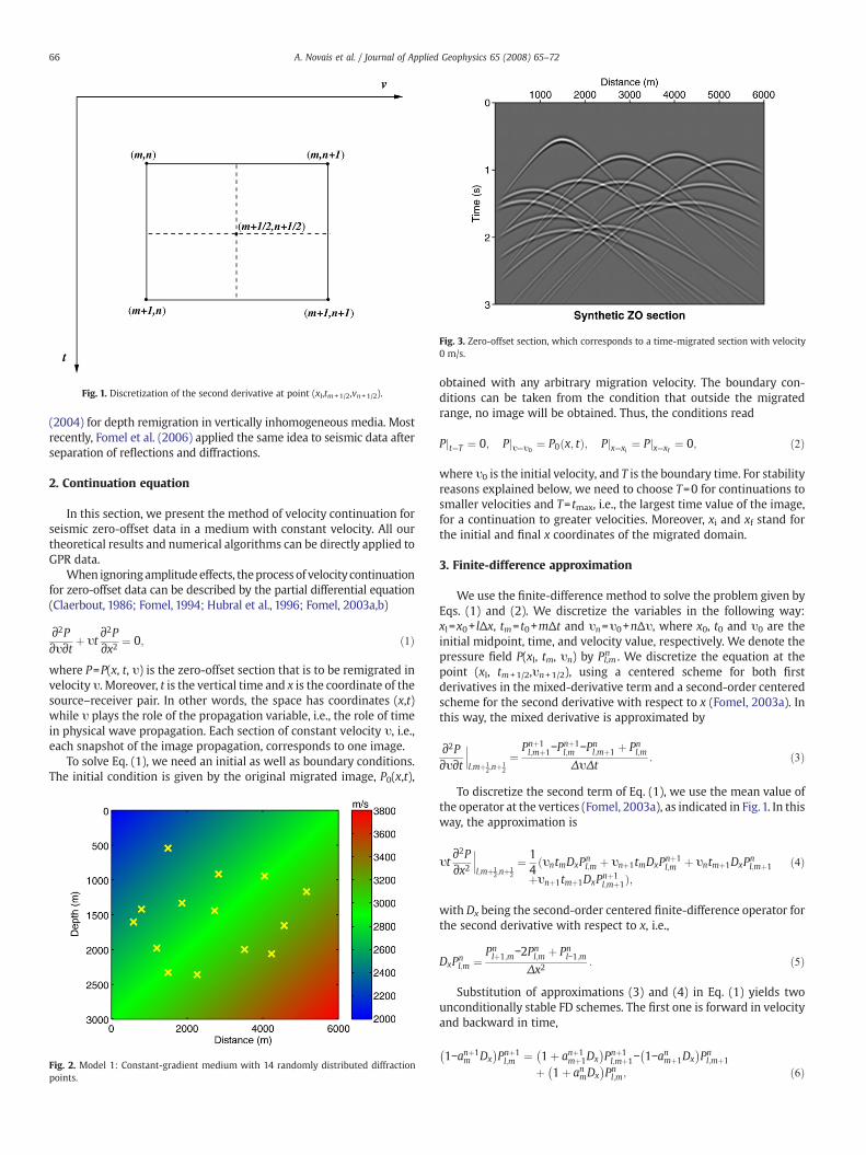
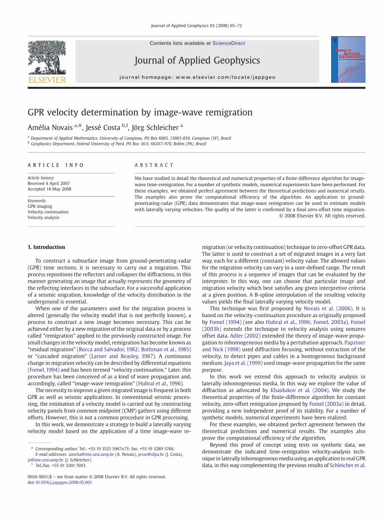
Fig. 1. Discretization of the second derivative at point (xl,tm +1/2,vn +1/2).

Fig. 3. Zero-offset section, which corresponds to a time-migrated section with velocity0 m/s.

66 A. Novais et al. / Journal of Applied Geophysics 65 (2008) 65–72

(2004) for depth remigration in vertically inhomogeneous media. Mostrecently, Fomel et al. (2006) applied the same idea to seismic data afterseparation of reflections and diffractions.

2. Continuation equation

In this section, we present the method of velocity continuation forseismic zero-offset data in a medium with constant velocity. All ourtheoretical results and numerical algorithms can be directly applied toGPR data.

When ignoringamplitudeeffects, theprocess of velocity continuationfor zero-offset data can be described by the partial differential equation(Claerbout, 1986; Fomel, 1994; Hubral et al., 1996; Fomel, 2003a,b)

∂2P∂υ∂t

þ υt∂2P∂x2

¼ 0; ð1Þ

where P=P(x, t, υ) is the zero-offset section that is to be remigrated invelocity υ. Moreover, t is the vertical time and x is the coordinate of thesource–receiver pair. In other words, the space has coordinates (x,t)while υ plays the role of the propagation variable, i.e., the role of timein physical wave propagation. Each section of constant velocity υ, i.e.,each snapshot of the image propagation, corresponds to one image.

To solve Eq. (1), we need an initial as well as boundary conditions.The initial condition is given by the original migrated image, P0(x,t),

Fig. 2. Model 1: Constant-gradient medium with 14 randomly distributed diffractionpoints.

obtained with any arbitrary migration velocity. The boundary con-ditions can be taken from the condition that outside the migratedrange, no image will be obtained. Thus, the conditions read

Pjt¼T ¼ 0; Pjυ¼υ0¼ P0 x; tð Þ; Pjx¼xi

¼ Pjx¼xf¼ 0; ð2Þ

where υ0 is the initial velocity, and T is the boundary time. For stabilityreasons explained below, we need to choose T=0 for continuations tosmaller velocities and T= tmax, i.e., the largest time value of the image,for a continuation to greater velocities. Moreover, xi and xf stand forthe initial and final x coordinates of the migrated domain.

3. Finite-difference approximation

We use the finite-difference method to solve the problem given byEqs. (1) and (2). We discretize the variables in the following way:xl =x0+ lΔx, tm= t0+mΔt and υn=υ0+nΔυ, where x0, t0 and υ0 are theinitial midpoint, time, and velocity value, respectively. We denote thepressure field P(xl, tm, υn) by Pl,m

n . We discretize the equation at thepoint (xl, tm+1/2,υn+1/2), using a centered scheme for both firstderivatives in the mixed-derivative term and a second-order centeredscheme for the second derivative with respect to x (Fomel, 2003a). Inthis way, the mixed derivative is approximated by

∂2P∂υ∂t jl;mþ1

2;nþ12

¼Pnþ1l;mþ1−P

nþ1l;m −Pn

l;mþ1 þ Pnl;m

ΔυΔt: ð3Þ

To discretize the second term of Eq. (1), we use the mean value ofthe operator at the vertices (Fomel, 2003a), as indicated in Fig.1. In thisway, the approximation is

υt∂2P∂x2 jl;mþ1

2;nþ12

¼ 14ðυntmDxPn

l;m þ υnþ1tmDxPnþ1l;m þ υntmþ1DxPn

l;mþ1

þυnþ1tmþ1DxPnþ1l;mþ1Þ;

ð4Þ

with Dx being the second-order centered finite-difference operator forthe second derivative with respect to x, i.e.,

DxPnl;m ¼ Pn

lþ1;m−2Pnl;m þ Pn

l−1;m

Δx2: ð5Þ

Substitution of approximations (3) and (4) in Eq. (1) yields twounconditionally stable FD schemes. The first one is forward in velocityand backward in time,

1−anþ1m Dx

� �Pnþ1l;m ¼ 1þ anþ1

mþ1Dx� �

Pnþ1l;mþ1− 1−anmþ1Dx

� �Pnl;mþ1

þ 1þ anmDx� �

Pnl;m; ð6Þ

Fig. 4. Remigration of synthetic diffraction data. Velocity is: (a) 2175 m/s; (b) 2275 m/s; (c) 2450 m/s; (d) 2600 m/s; (e) 2750 m/s; and (f) 2850 m/s.

67A. Novais et al. / Journal of Applied Geophysics 65 (2008) 65–72

where amn =(υntmΔυΔt)/4. The second scheme is forward in time and

backward in velocity,

1−anmþ1Dx� �

Pnl;mþ1 ¼ 1þ anþ1

mþ1Dx� �

Pnþ1l;mþ1− 1−anþ1

m Dx� �

Pnþ1l;m þ 1þ anmDx

� �Pnl;m; ð7Þ

with the same amn . As demonstrated in the next section, scheme (6) is

unconditionally stable for increasing velocity and decreasing time,while scheme (7) is unconditionally stable for decreasing velocity andincreasing time.

In this work, we have implemented scheme (6), which is moreconvenient to describe a practical time-remigration, since a zero-offset section can be thought of as a time-migrated section with zero

migration velocity (Chun and Jacewitz, 1981). An early implementa-tion of an implicit FD scheme for the velocity-continuation equationwas realized by Li (1986).

3.1. Numerical stability

To analyze the numerical stability of scheme (6), we use the vonNeumann criterion (Strikwerda, 1989; Thomas, 1995). This consists ofsubstituting

Pnl;m ¼ nnexp i lθx þmθtð Þð Þ ð8Þ

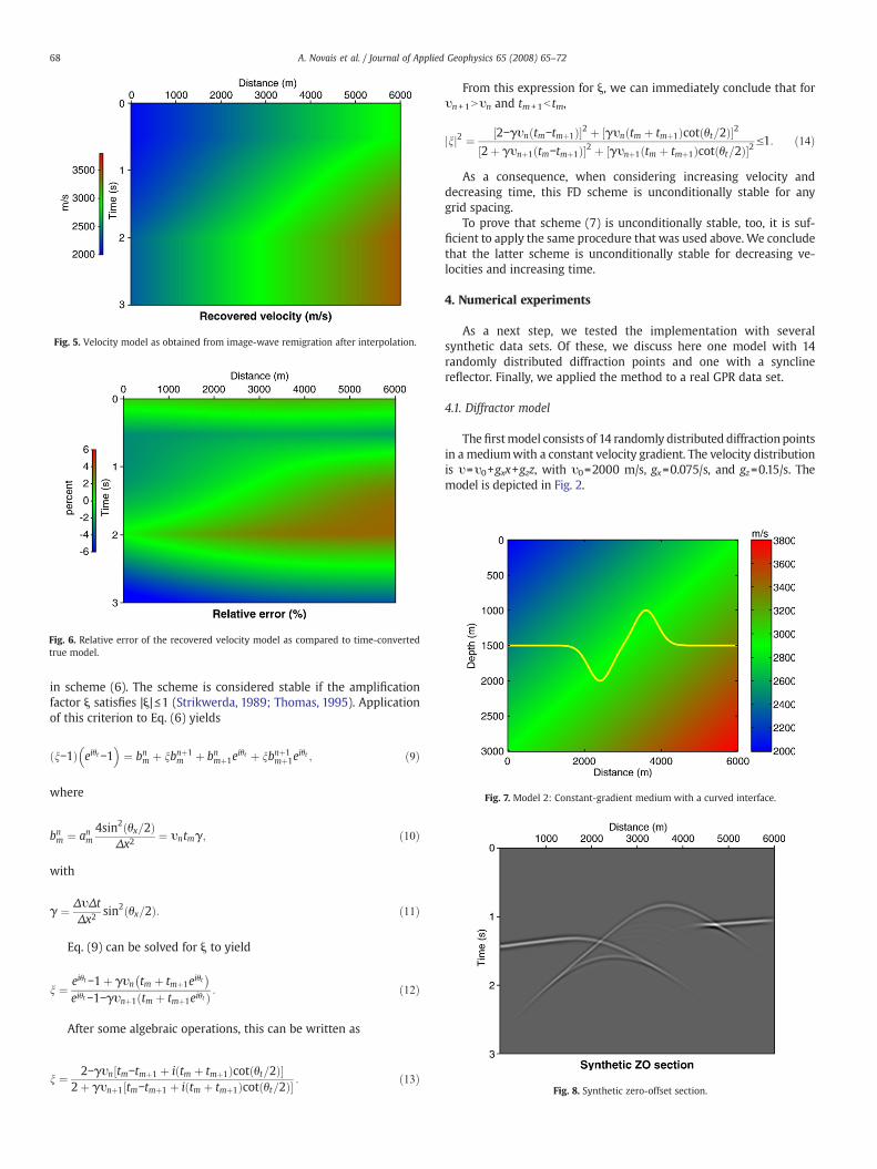
Fig. 5. Velocity model as obtained from image-wave remigration after interpolation.

Fig. 6. Relative error of the recovered velocity model as compared to time-convertedtrue model.

Fig. 7. Model 2: Constant-gradient medium with a curved interface.

Fig. 8. Synthetic zero-offset section.

68 A. Novais et al. / Journal of Applied Geophysics 65 (2008) 65–72

in scheme (6). The scheme is considered stable if the amplificationfactor ξ satisfies |ξ|≤1 (Strikwerda, 1989; Thomas, 1995). Applicationof this criterion to Eq. (6) yields

n−1ð Þ eiθt−1� �

¼ bnm þ nbnþ1m þ bnmþ1e

iθt þ nbnþ1mþ1e

iθt ; ð9Þ

where

bnm ¼ anm4sin2 θx=2ð Þ

Δx2¼ υntmγ; ð10Þ

with

γ ¼ ΔυΔtΔx2

sin2 θx=2ð Þ: ð11Þ

Eq. (9) can be solved for ξ to yield

n ¼ eiθt−1þ γυn tm þ tmþ1eiθt� �

eiθt−1−γυnþ1 tm þ tmþ1eiθtð Þ : ð12Þ

After some algebraic operations, this can be written as

n ¼ 2−γυn tm−tmþ1 þ i tm þ tmþ1ð Þcot θt=2ð Þ½ �2þ γυnþ1 tm−tmþ1 þ i tm þ tmþ1ð Þcot θt=2ð Þ½ � : ð13Þ

From this expression for ξ, we can immediately conclude that forυn+1Nυn and tm+1b tm,

jnj2 ¼ 2−γυn tm−tmþ1ð Þ½ �2 þ γυn tm þ tmþ1ð Þcot θt=2ð Þ½ �22þ γυnþ1 tm−tmþ1ð Þ½ �2 þ γυnþ1 tm þ tmþ1ð Þcot θt=2ð Þ½ �2

V1: ð14Þ

As a consequence, when considering increasing velocity anddecreasing time, this FD scheme is unconditionally stable for anygrid spacing.

To prove that scheme (7) is unconditionally stable, too, it is suf-ficient to apply the same procedure that was used above.We concludethat the latter scheme is unconditionally stable for decreasing ve-locities and increasing time.

4. Numerical experiments

As a next step, we tested the implementation with severalsynthetic data sets. Of these, we discuss here one model with 14randomly distributed diffraction points and one with a synclinereflector. Finally, we applied the method to a real GPR data set.

4.1. Diffractor model

The firstmodel consists of 14 randomly distributed diffractionpointsin a mediumwith a constant velocity gradient. The velocity distributionis υ=υ0+gxx+gzz, with υ0=2000 m/s, gx=0.075/s, and gz=0.15/s. Themodel is depicted in Fig. 2.

69A. Novais et al. / Journal of Applied Geophysics 65 (2008) 65–72

The corresponding zero-offset section was modeled by finitedifferences with a Ricker source pulse with a dominant frequency of31.25 Hz. For the zero-offset simulation, 601 source-receiver pairswere distributed along the surface between x=0 m and x=6000 m,regularly spaced at a distance of 10 m. The sampling rate was 2 ms.

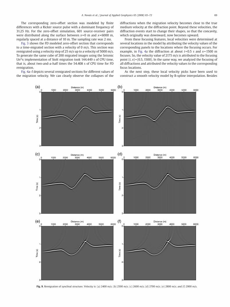
Fig. 3 shows the FD modeled zero-offset section that correspondsto a time-migrated section with a velocity of 0 m/s. This section wasremigrated using a velocity step of 25 m/s up to a velocity of 5000m/s.To generate the same cube of 200 migrated images using the SeismicUn⁎x implementation of Stolt migration took 144.449 s of CPU time,that is, about two-and-a-half times the 54.408 s of CPU time for FDremigration.

Fig. 4a–f depicts several remigrated sections for different values ofthe migration velocity. We can clearly observe the collapses of the

Fig. 9. Remigration of synclinal structure. Velocity is: (a) 2400 m/s; (b) 25

diffractions when the migration velocity becomes close to the truemedium velocity at the diffraction point. Beyond these velocities, thediffraction events start to change their shapes, so that the concavity,which originally was downward, now becomes upward.

From these focusing features, local velocities were determined atseveral locations in the model by attributing the velocity values of thecorresponding panels to the locations where the focusing occurs. Forexample, in Fig. 4a the diffraction at about t=0.5 s and x=1500 mfocuses. So, the velocity value of 2175 m/s is attributed to the focusingpoint (t, x)=(0.5, 1500). In the same way, we analyzed the focusing ofall diffractions and attributed the velocity values to the correspondingfocus locations.

As the next step, these local velocity picks have been used toconstruct a smooth velocity model by B-spline interpolation. Besides

00 m/s; (c) 2600 m/s; (d) 2700 m/s; (e) 2800 m/s; and (f) 2900 m/s.

70 A. Novais et al. / Journal of Applied Geophysics 65 (2008) 65–72

fitting the sampled values in the least squares sense, minimumgradient and curvature constraints were applied in order to obtain aunique interpolation (Menke, 1989). The resulting velocity model isdepicted in Fig. 5.

Note that the velocity gradient is rather well reconstructed in thepart of the model where diffractions were located. To better under-stand the quality of the velocity analysis, we calculated the relativeerror (see Fig. 6) from the time-converted original velocity model ofFig. 2. The conversionwas done using Seismic Un⁎x.Within the part ofthe model where diffraction data are available, the relative velocityerror is below 2.5%.

4.2. Synclinal model

Our second test with synthetic data is to apply the image-wavevelocity continuation to a model where the wavefield has passedthrough a caustic. The second model can be seen in Fig. 7. The zero-offset section is depicted in Fig. 8, where the CMP spacing was chosenas 10 m. The source pulse was again a Ricker wavelet, again with adominant frequency of 31.25 Hz. The background medium is the sameconstant-gradient medium of Model 1, in which a curved interface isembedded. The zero-offset section was simulated using the explod-ing-reflector model (Loewenthal et al., 1976). Since the reflectorcontains a synclinal structure, the zero-offset section presents thewell-known bow-tie structure.

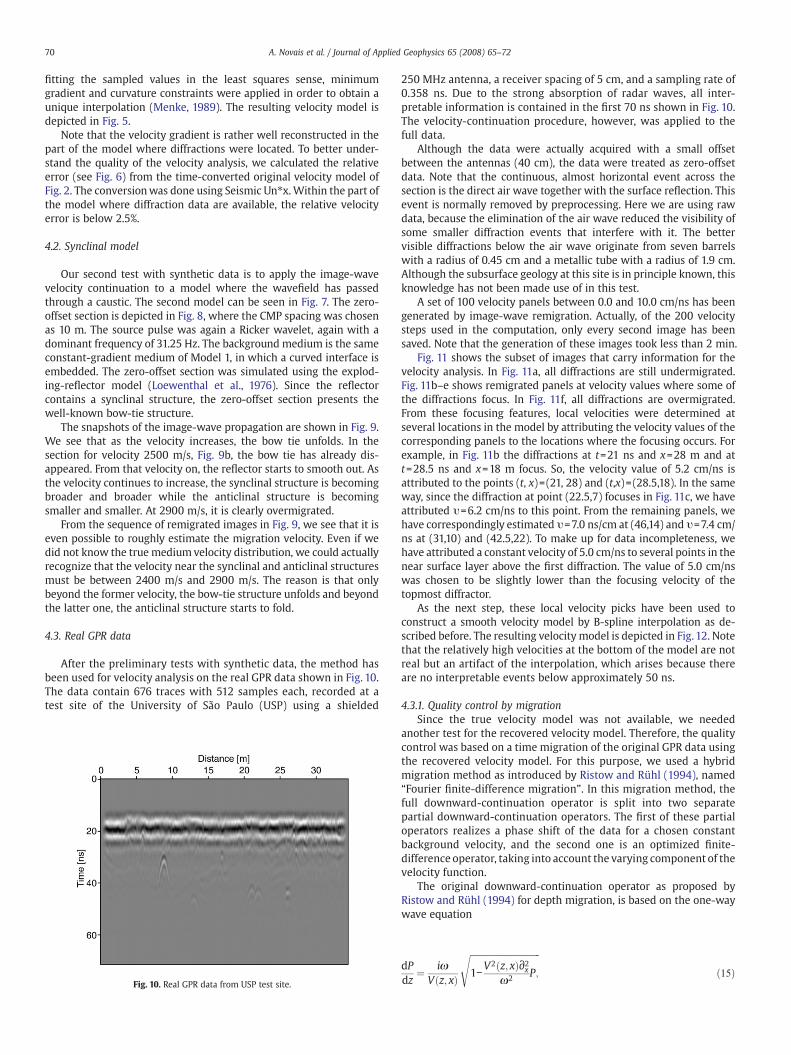
The snapshots of the image-wave propagation are shown in Fig. 9.We see that as the velocity increases, the bow tie unfolds. In thesection for velocity 2500 m/s, Fig. 9b, the bow tie has already dis-appeared. From that velocity on, the reflector starts to smooth out. Asthe velocity continues to increase, the synclinal structure is becomingbroader and broader while the anticlinal structure is becomingsmaller and smaller. At 2900 m/s, it is clearly overmigrated.

From the sequence of remigrated images in Fig. 9, we see that it iseven possible to roughly estimate the migration velocity. Even if wedid not know the true medium velocity distribution, we could actuallyrecognize that the velocity near the synclinal and anticlinal structuresmust be between 2400 m/s and 2900 m/s. The reason is that onlybeyond the former velocity, the bow-tie structure unfolds and beyondthe latter one, the anticlinal structure starts to fold.

4.3. Real GPR data

After the preliminary tests with synthetic data, the method hasbeen used for velocity analysis on the real GPR data shown in Fig. 10.The data contain 676 traces with 512 samples each, recorded at atest site of the University of São Paulo (USP) using a shielded

Fig. 10. Real GPR data from USP test site.

250 MHz antenna, a receiver spacing of 5 cm, and a sampling rate of0.358 ns. Due to the strong absorption of radar waves, all inter-pretable information is contained in the first 70 ns shown in Fig. 10.The velocity-continuation procedure, however, was applied to thefull data.

Although the data were actually acquired with a small offsetbetween the antennas (40 cm), the data were treated as zero-offsetdata. Note that the continuous, almost horizontal event across thesection is the direct air wave together with the surface reflection. Thisevent is normally removed by preprocessing. Here we are using rawdata, because the elimination of the air wave reduced the visibility ofsome smaller diffraction events that interfere with it. The bettervisible diffractions below the air wave originate from seven barrelswith a radius of 0.45 cm and a metallic tube with a radius of 1.9 cm.Although the subsurface geology at this site is in principle known, thisknowledge has not been made use of in this test.

A set of 100 velocity panels between 0.0 and 10.0 cm/ns has beengenerated by image-wave remigration. Actually, of the 200 velocitysteps used in the computation, only every second image has beensaved. Note that the generation of these images took less than 2 min.

Fig. 11 shows the subset of images that carry information for thevelocity analysis. In Fig. 11a, all diffractions are still undermigrated.Fig. 11b–e shows remigrated panels at velocity values where some ofthe diffractions focus. In Fig. 11f, all diffractions are overmigrated.From these focusing features, local velocities were determined atseveral locations in the model by attributing the velocity values of thecorresponding panels to the locations where the focusing occurs. Forexample, in Fig. 11b the diffractions at t=21 ns and x=28 m and att=28.5 ns and x=18 m focus. So, the velocity value of 5.2 cm/ns isattributed to the points (t, x)=(21, 28) and (t,x)=(28.5,18). In the sameway, since the diffraction at point (22.5,7) focuses in Fig. 11c, we haveattributed υ=6.2 cm/ns to this point. From the remaining panels, wehave correspondingly estimated υ=7.0 ns/cm at (46,14) and υ=7.4 cm/ns at (31,10) and (42.5,22). To make up for data incompleteness, wehave attributed a constant velocity of 5.0 cm/ns to several points in thenear surface layer above the first diffraction. The value of 5.0 cm/nswas chosen to be slightly lower than the focusing velocity of thetopmost diffractor.

As the next step, these local velocity picks have been used toconstruct a smooth velocity model by B-spline interpolation as de-scribed before. The resulting velocity model is depicted in Fig. 12. Notethat the relatively high velocities at the bottom of the model are notreal but an artifact of the interpolation, which arises because thereare no interpretable events below approximately 50 ns.

4.3.1. Quality control by migrationSince the true velocity model was not available, we needed

another test for the recovered velocity model. Therefore, the qualitycontrol was based on a time migration of the original GPR data usingthe recovered velocity model. For this purpose, we used a hybridmigration method as introduced by Ristow and Rühl (1994), named“Fourier finite-difference migration”. In this migration method, thefull downward-continuation operator is split into two separatepartial downward-continuation operators. The first of these partialoperators realizes a phase shift of the data for a chosen constantbackground velocity, and the second one is an optimized finite-difference operator, taking into account the varying component of thevelocity function.

The original downward-continuation operator as proposed byRistow and Rühl (1994) for depth migration, is based on the one-waywave equation

dPdz

¼ iωV z; xð Þ

ffiffiffiffiffiffiffiffiffiffiffiffiffiffiffiffiffiffiffiffiffiffiffiffiffiffiffiffiffiffiffiffi1−

V2 z; xð Þ∂2xω2 P;

sð15Þ

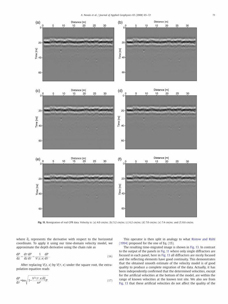
Fig. 11. Remigration of real GPR data. Velocity is: (a) 4.0 cm/ns; (b) 5.2 cm/ns; (c) 6.2 cm/ns; (d) 7.0 cm/ns; (e) 7.4 cm/ns; and (f) 8.6 cm/ns.

71A. Novais et al. / Journal of Applied Geophysics 65 (2008) 65–72

where ∂x represents the derivative with respect to the horizontalcoordinate. To apply it using our time-domain velocity model, weapproximate the depth derivative using the chain rule as

dPdz

¼ dτdz

dPdτ

¼ 1V z; xð Þ

dPdτ

: ð16Þ

After replacing V(z, x) by V(τ, x) under the square root, the extra-polation equation reads

dPdτ

≈iω

ffiffiffiffiffiffiffiffiffiffiffiffiffiffiffiffiffiffiffiffiffiffiffiffiffiffiffiffiffiffiffiffi1−

V2 τ; xð Þ∂2xω2 P:

sð17Þ

This operator is then split in analogy to what Ristow and Rühl(1994) proposed for the one of Eq. (15).

The resulting time-migrated image is shown in Fig. 13. In contrastto the output of the panels in Fig. 11 where only single diffractors arefocused in each panel, here in Fig. 13 all diffractors are nicely focusedand the reflecting elements have good continuity. This demonstratesthat the obtained smooth estimate of the velocity model is of goodquality to produce a complete migration of the data. Actually, it hasbeen independently confirmed that the determined velocities, exceptfor the artificial velocities at the bottom of the model, are within therange of known velocities at the known test site. We also see fromFig. 13 that these artificial velocities do not affect the quality of the

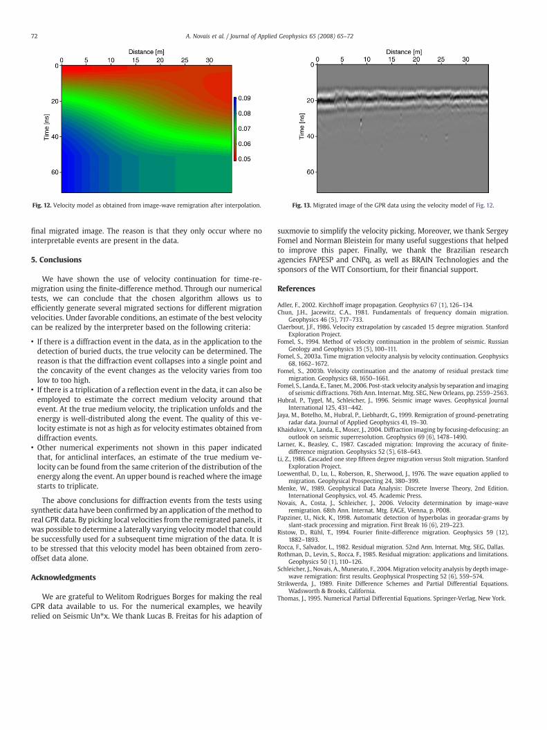
Fig. 12. Velocity model as obtained from image-wave remigration after interpolation. Fig. 13. Migrated image of the GPR data using the velocity model of Fig. 12.

72 A. Novais et al. / Journal of Applied Geophysics 65 (2008) 65–72

final migrated image. The reason is that they only occur where nointerpretable events are present in the data.

5. Conclusions

We have shown the use of velocity continuation for time-re-migration using the finite-difference method. Through our numericaltests, we can conclude that the chosen algorithm allows us toefficiently generate several migrated sections for different migrationvelocities. Under favorable conditions, an estimate of the best velocitycan be realized by the interpreter based on the following criteria:

• If there is a diffraction event in the data, as in the application to thedetection of buried ducts, the true velocity can be determined. Thereason is that the diffraction event collapses into a single point andthe concavity of the event changes as the velocity varies from toolow to too high.

• If there is a triplication of a reflection event in the data, it can also beemployed to estimate the correct medium velocity around thatevent. At the true medium velocity, the triplication unfolds and theenergy is well-distributed along the event. The quality of this ve-locity estimate is not as high as for velocity estimates obtained fromdiffraction events.

• Other numerical experiments not shown in this paper indicatedthat, for anticlinal interfaces, an estimate of the true medium ve-locity can be found from the same criterion of the distribution of theenergy along the event. An upper bound is reached where the imagestarts to triplicate.

The above conclusions for diffraction events from the tests usingsynthetic data have been confirmed by an application of themethod toreal GPR data. By picking local velocities from the remigrated panels, itwas possible to determine a laterally varying velocitymodel that couldbe successfully used for a subsequent time migration of the data. It isto be stressed that this velocity model has been obtained from zero-offset data alone.

Acknowledgments

We are grateful to Welitom Rodrigues Borges for making the realGPR data available to us. For the numerical examples, we heavilyrelied on Seismic Un⁎x. We thank Lucas B. Freitas for his adaption of

suxmovie to simplify the velocity picking. Moreover, we thank SergeyFomel and Norman Bleistein for many useful suggestions that helpedto improve this paper. Finally, we thank the Brazilian researchagencies FAPESP and CNPq, as well as BRAIN Technologies and thesponsors of the WIT Consortium, for their financial support.

References

Adler, F., 2002. Kirchhoff image propagation. Geophysics 67 (1), 126–134.Chun, J.H., Jacewitz, C.A., 1981. Fundamentals of frequency domain migration.

Geophysics 46 (5), 717–733.Claerbout, J.F., 1986. Velocity extrapolation by cascaded 15 degree migration. Stanford

Exploration Project.Fomel, S., 1994. Method of velocity continuation in the problem of seismic. Russian

Geology and Geophysics 35 (5), 100–111.Fomel, S., 2003a. Time migration velocity analysis by velocity continuation. Geophysics

68, 1662–1672.Fomel, S., 2003b. Velocity continuation and the anatomy of residual prestack time

migration. Geophysics 68, 1650–1661.Fomel, S., Landa, E., Taner,M., 2006. Post-stack velocity analysis by separation and imaging

of seismic diffractions. 76th Ann. Internat. Mtg. SEG, NewOrleans, pp. 2559–2563.Hubral, P., Tygel, M., Schleicher, J., 1996. Seismic image waves. Geophysical Journal

International 125, 431–442.Jaya, M., Botelho, M., Hubral, P., Liebhardt, G., 1999. Remigration of ground-penetrating

radar data. Journal of Applied Geophysics 41, 19–30.Khaidukov, V., Landa, E., Moser, J., 2004. Diffraction imaging by focusing-defocusing: an

outlook on seismic superresolution. Geophysics 69 (6), 1478–1490.Larner, K., Beasley, C., 1987. Cascaded migration: Improving the accuracy of finite-

difference migration. Geophysics 52 (5), 618–643.Li, Z., 1986. Cascaded one step fifteen degree migration versus Stolt migration. Stanford

Exploration Project.Loewenthal, D., Lu, L., Roberson, R., Sherwood, J., 1976. The wave equation applied to

migration. Geophysical Prospecting 24, 380–399.Menke, W., 1989. Geophysical Data Analysis: Discrete Inverse Theory, 2nd Edition.

International Geophysics, vol. 45. Academic Press.Novais, A., Costa, J., Schleicher, J., 2006. Velocity determination by image-wave

remigration. 68th Ann. Internat. Mtg. EAGE, Vienna, p. P008.Papziner, U., Nick, K., 1998. Automatic detection of hyperbolas in georadar-grams by

slant-stack processing and migration. First Break 16 (6), 219–223.Ristow, D., Rühl, T., 1994. Fourier finite-difference migration. Geophysics 59 (12),

1882–1893.Rocca, F., Salvador, L., 1982. Residual migration. 52nd Ann. Internat. Mtg. SEG, Dallas.Rothman, D., Levin, S., Rocca, F., 1985. Residual migration: applications and limitations.

Geophysics 50 (1), 110–126.Schleicher, J., Novais, A., Munerato, F., 2004. Migration velocity analysis by depth image-

wave remigration: first results. Geophysical Prospecting 52 (6), 559–574.Strikwerda, J., 1989. Finite Difference Schemes and Partial Differential Equations.

Wadsworth & Brooks, California.Thomas, J., 1995. Numerical Partial Differential Equations. Springer-Verlag, New York.