Accuracy of arterial pulse-wave velocity measurement using MR

Original Research

Accuracy of Arterial Pulse-Wave Velocity Measurement Using MR

Bradley D. Bolster, Jr, MSE Ergin Atalar, PhD

The performance of a one-dimensional MR technique for the estimation of pulse-wave velocity in the aorta was evaluated. An expression for the error in this estimate was formulated and veri5ed both by simulation and by experiment. On the basis of this formulation. guidelines for increasing the emciency of the acquisition were established. The technique was further vali- dated by comparison with pulse-wave velocity measurements made with a pressure catheter. All data were acquired from a latex tube driven by a pulsatile flow system. MR measurements of pulse-wave velocity in the tube were found to be very reproducible in the presence of white noise. Measurements by other techniques were in good agreement, falling within 2 SD of the mean. Because of its sensitivity and spatial resolution. this technique shows promise for making spatially resolved estimates of vessel distensibility. This would allow assessment of diseases, such as atherosclerosis, that cause local changes in the material properties of the vasculature.

Index t e r n : aortlc compliance * pulse-wave velocity * MFU

JHRl lssB: 8:87a888

Abbreviations: 1D = one-dimensional, SNR = signal-to-noise ratio

From the Departments of Biomedical Engineering (B.D.B., E.RM.1 and Ra- diology (E.A.. E.R.M.), Johns Hopkins University Schwl of Medicine, Balti- more, MD: GE Colporate Research and Development Center, Schenectady. NY (C.J.H.). E-mail: e a M m r i . j h u . e d u . Received July 17. 1997: rwision requested October 1, 1997; rwision received November 26. 1997: accepted December 18. 1997. This work was supported by a Whitaker Foundation Bio- medical Research Grant. Dr Atalar was supported by a Frank McClure Fel- lowship. Presented. in part, at the Society of Magnetic Resonance/European Society for Magnetic Resonance in Medicine and Biology joint meeUng in Nice. France, August 19-25, 1995. M d n ~ reprint requests to E.A., Johns Hop- kins Outpatient Center Roam 4241, 601 N. Caroline Street, Baltimore, MD 21287-0845.

Christopher J. Hardy, PhD Elliot R. McVeigh, PhD

THE DISTENSIBILITY OF the aorta plays an important role in smoothing the blood flow delivered to the periph- ery and maintaining this flow during diastole (1). This is achieved by the reduction of the mechanical impedance seen by the ejecting left ventricle (2-4). Changes in aortic distensibility appear to correlate with age, coronary artery disease, and fitness (5-7). Specifically, particular changes have been attributed to the presence of atherosclerosis (8,9) or connective tissue disorders (10-12). Chronic increased vascular loading may lead to left ven- tricular hypertrophy and even heart failure, whereas changes in the material properties of the aortic wall and accompanying aneurysmal dilation commonly lead to sudden aortic dissection or rupture. An accurate, noninvasive method to estimate the material properties of the aortic wall could play an important role in the early diagnosis of vascular disease such as atherosclerosis and provide a guideline for surgical intervention in cases of aneurysmal dilation.

The distensibility of blood vessels can be measured directly by imaging the fractional change in cross-sectional area of the vessel with given changes in pressure. This measurement has been made with cine x-ray angiog- raphy (13), ultrasound (14.151, x-ray CT (16), and MRI (6) coupled with either sphygmomanometer- or microman- ometer-based blood pressure measurements. Low image resolution, motion, and the lack of local blood pressure measurements increase the error of these techniques. Estimates of blood vessel distensibility have also been obtained by measurements of pulse-wave velocity in the aorta. The pulse-wave velocity is the rate at which a flow or pressure wave propagates down a vessel. It is directly related to the elasticity of the vessel wall (1 7) and can be estimated by measuring the transit time of the pulse wave between two points a known distance apart. Inva- sive techniques using pressure catheters are historically the “gold standard for such measurements, but recently, noninvasive measurements have been made with Dopp- ler ultrasound (18) and MR (19-22). Ultrasound is limited because of the small availability of acoustic windows along the length of the aorta and the inability to spatially register different velocity measurements accurately, whereas MR can access the entire length of the aorta and provide very accurate spatial registration of the resulting data.

Pulse-wave velocity has been used to follow the progression of some arterial diseases. In monkeys, for example, it was found that aortic pulse-wave velocity increased almost 40% with increasing atherosclerotic

878

load (9). albeit accompanied by an almost 50% stenosis. Marfan syndrome patients have been studied as well and exhibited pulse-wave velocities that were 20% above normal (12). Hypertension has also been shown to elevate pulse-wave velocity in the human aorta (23). To be useful in the study of disease and ultimately have some clinical application, a technique must produce measurements that have less variation than the changes that occur in pathological states. Reproducibility studies with Doppler ultrasound show sensitivity to transducer placement and angle, factors that affect the apparent path length of the pulse wave. These studies seem to suggest normal pulse- wave velocity measurement variations between 10% and 20% (18,24). Clearly, in vivo reproducibility must be improved to provide reliable detection and monitoring of disease states.

Diseases such as atherosclerosis affect the human aortic wall in very localized regions. The formation of plaque changes the mechanical properties of the wall (8). pro- gressively altering these properties with changes in plaque composition (25). Hence, the presence of early- stage atherosclerosis may potentially be detectable as a local change in vessel distensibility, and it is therefore preferable that the technique applied make distensibility measurements in a spatially resolved manner.

In this article, we investigate the accuracy of the one- dimensional (1D) NMR pulse-wave velocity technique (19) and some error sources that influence the quality of pulse-wave velocity estimates made from its measurements. A theoretical lower error bound will be established for these MR-based pulse-wave velocity measurements, and we show both in simulations and in experiments that, coupled with a matched filtering analysis technique, estimates obtained with the 1D NMR pulse-wave velocity technique achieve this lower error bound. Because of its error performance, its ability to provide data with high temporal and spatial resolution from a known anatomic location, and its promise for enabling local measurements of vessel wall properties not possible with other noninvasive techniques, the 1D MR pulse-wave velocity measurement technique shows strong potential in meeting the requirements of a reliable in vivo measurement technique.

0 THEORY

Measurement Model Blood vessels are often modeled as homogeneous elas-

tic tubes in which velocity waves obey the 1D wave equation (1 7). In the context of the aorta, the solution to this wave equation is the sum of a forward-moving wave orig- inating at the heart and a backward-moving wave caused by wave reflections from points downstream of the measurement area, such as branch points and the high-impedance arterioles. As a result of the nonuniform branch- ing of the arterial tree, however, the high-frequency components in the reflected waves from multiple periph- eral branch sites tend to either interfere destructively with each other through end diastole or become trapped in smaller vessels because of the directional sensitivity of reflection coefficients at branch points (1). These effects cause high-frequency reflections to represent an insig- nificant portion of the onset of the next pulse waveform. The foot of the flow waveform, the point at which it begins its sharp upslope, is a high-frequency feature. If the scope of the estimation technique is limited to the foot, reflections can be assumed to be negligible for the pur-

poses of pulse-wave velocity estimation (1,2). We can then model the velocity as a function of position along the vessel and time, zl(x,t), with the forward-moving portion of the wave equation solution:

X

C Dc., (x, t) - u (t - - - tJ.

t,, in this equation is the temporal position of the foot of the wave front at x = 0. c is the pulse-wave velocity, the parameter being estimated. In using this model, we assume that the pulse-wave velocity is constant over the region of vessel being studied. This implies that across this region, neither the material properties of the vessel wall nor the cross-sectional area of the vessel changes.

earner-Rao Lower Error Bound for the Estimation of Pulse-Wave Velocity

With phase-contrast techniques, the phase of the MR signal is linearly related to the velocity of the spins being measured. Under these conditions, the MR signal sampled with a temporal sampling period, At, and a spatial sampling period, Ax, with respective sample indices nand m is

where & and 9, are the amplitude and phase of the MR signal independent of flow velocity, 9- is the phase angle at the maximum velocity, urn, Y, is zero mean additive gaussian noise, and j = m. Once phase-difference reconstruction is performed, the noise in the signal is no longer gaussian. For the Cramer-Rao bound to be valid, the analysis must be performed on the raw MR data. As seen in Equation [2], the relationship between the pulse-wave velocity and the raw MR signal is not a linear one. Hence, the problem of calculating pulse-wave velocity given the MR data becomes a nonlinear parameter estimation problem.

As detailed in the Appendix, the Cramer-Rao lower error bound (26) for the estimation of pulse-wave velocity, c, can be written as

u > q-- . (3) - SNR 4- L3 j-?: [u’ ( 7 ) / u J 2 d7

This measurement is made over vessel length, L. u’ /u- is the temporal derivative of the velocity waveform normalized to the maximum velocity and signal-to-noise ratio (SNR) = the magnitude image SNR. This expression is valid if the sampling of velocity is above the Nyquist rate in both the temporal and spatial directions. For the purpose of elucidating the effect of the acquisition parameters, the expression in Equation [3] can be simplified by assuming that the velocity waveform is a ramp of constant slope and duration k,:

(4)

Here, Le is defined as 50% to 75% of the total velocity rise time, because this portion of the waveform is least affected by reflections ( 17). The Cramer-Rao lower bound gives the minimum possible error of any estimation technique. It is a useful quantity only if a parameter estimation algorithm that satisfies the bound with equality can be found. Such an estimator is known as an efficient estimator (26). We describe and validate such an algorithm in the following sections. Because our estimator is efficient, the expression in Equation 141 becomes an equality

Volume 8 Number 4 JMRl 879

and can be used to illustrate some important guidelines for the acquisition of MR data used for calculating pulse- wave velocity. Only three quantities in Equation [4] are directly con-

trollable by the acquisition: temporal resolution, spatial resolution, and +- Since SNR a <&, where & is the MR signal readout time (27). using Equation [4] we can put forth some guidelines for making the 1D MR acquisition more efficient. For example, increasing temporal resolution above the Nyquist rate is equivalent to averaging data at the original temporal resolution, whereas increasing the spatial resolution, ie, decreasing h, by increasing the readout time had no effect on the pulse-wave velocity estimation error. This implies that one can shorten the data acquisition window to obtain minimum resolution without losing any information about pulse-wave velocity. Minimum resolution in this case is the smaller of either the Nyquist limit or the min- imal necessary spatial resolution for the pulse-wave velocity measurement. The Nyquist limit for spatial resolution is governed by the true pulse-wave velocity in the vessel. As in MR imaging, if spatial resolution is increased by decreasing the field of view (ie, increasing the strength of the readout gradient), reduction of the voxel volume without increasing the imaging time degrades the SNR and the pulse-wave velocity estimation error increases.

The sensitivity of the velocity-encoding gradient should be maximimd, even if this results in velocity aliasing. At the very least, a phase of T should correspond with the initial 50% to 75% of the velocity upstroke, so the portion of the waveform least sensitive to reflections spans the entire dynamic range of velocity values. This increases +- to T , reducing the pulse-wave velocity estimation error. Because the velocity waveform is smoothly mono- tonic in the foot region, it is possible that a phase-un- wrapping algorithm could allow a further increase in +- The tradeoff in increasing +- is the increased duration of the velocity-encoding gradient. Depending on the ca- pabilities of the gradient subsystem, increasing the area of the velocity-encoding gradient could require increasing its duration. In this case, the most prominent effect would be an increase in TR and therefore an increase in imaging time.

For typical acquisition parameters, such as a temporal resolution of 2 msec, a spatial resolution of 1 mm, and a measurable vessel length of 10 cm, at a pulse-wave velocity of 500 cm/sec and a typical SNR of 20, the estimation error is <.5%. This value is already much less than the typical physiological variability. With the same imaging parameters, pulse-wave velocity can be measured for l .4 cm of vessel with 10% accuracy. This shows the potential of this technique for the measurement of truly local pulse-wave velocity.

. IMETHoDs 1D NMR Velocity Acquisition Technique

We collected M R data for the estimation of pulse-wave velocity using a 1D velocity technique (19). The pulse sequence consisted of a modified gradient echo sequence with a TR = 32 msec. as shown in Figure 1. This acquisition was prospectively gated to the cardiac cycle, and 16 phases were acquired during each cardiac cycle. The slice selection was replaced with a cylindrical excitation pulse using a spiral k-space trajectory (28.29). This resulted in a cylinder-shaped region from which the MR signal was

elicited that was oriented coaxial to a chosen straight length of the blood vessel. The readout gradient was oriented along its axis. A bipolar flow-encoding gradient was added in the flow direction, and phase contrast acquisition was performed. The polarity of the flow-encoding gradient was flipped for every other cardiac cycle, and phase-difference reconstruction was applied. By incrementing the delay after the cardiac tngger by 2 msec for subsequent cardiac cycle pairs, the acquisition collected S,, with 2- msec temporal resolution and 1. l-mm spatial resolution in 32 cardiac cycles. In some cases, Sm, was collected with l-msec temporal resolution in 64 cardiac cycles.

Estimation of Pulse-Wave Velocity ftom the MR Velocity Data

Once S,, was collected, we found the temporal position of the velocity waveform as a function of position by min- imizing the mean square error between a predescribed template and the leading edge of the velocity waveform in the temporal direction. This is shown in Figure 2. Then, the resulting temporal-spatial pairs were subjected to l i i - ear regression, the slope of which yielded the estimated pulse-wave velocity. To assess the quality of the pulse- wave velocity estimate, 95% confidence intervals were also calculated for the slope of the fit. Representative position versus time data and the resulting pulse-wave velocity estimate are shown in Figure 3.

SIMULATIONS The variance on the error of any estimation technique

cannot be lower than the Cramer-Rao bound. An efficient estimator satisfies this lower bound with equality. By showing that our estimation algorithm is efficient, we im- ply that no other algorithm can make better estimates of pulse-wave velocity from the data. For this purpose, we compared the performance of our analysis technique with the Cramer-Rao bound in the presence of measurement noise by Monte Carlo simulations.

The simulation consisted of three stages: First, from the wave equation solution of Equation [ 11, the propaga- tion of an initial flow waveform down the vessel was calculated, in the absence of reflections. Second, from the simulated flow data, the resulting complex MR signals were calculated and gaussian measurement noise was added, which resulted in the MR data, kn. The phase of these simulated MR data was calculated, followed by matched filtering analysis. A block diagram of the simulation steps is shown in Figure 4.

To check sensitivity to measurement noise, the Monte Carlo aspect of the simulation consisted of varying the measurement noise and repeating the reconstruction and analysis. The estimation error was designated as the difference between the true pulse-wave velocity used to gen- erate the data, Is,,, and the resulting estimated value.

The noiseless pulse-wave velocity data were generated by applying Equation [ 11 to a computer-generated ramp function.

i f t l t , u,(d = a, ( t - iLJ for t, I t I (2) + t, (5)

The rise time of this waveform was chosen to be 20 msec, similar to what is seen physiologically at the foot of a typical human aortic flow waveform. With u,, arbitrarily set to 1 cm/sec, this corresponded to a, = 50 cm/sec2 in Equation IS].

Velocity data sets, S,,, were calculated for several pulse-wave velocity values (100,250.500, and 1,000 cm/

{I- otherwise

880 JMRl July/August 1998

I- - I , , . I . . . . , ,

10.0 20.0 30.0 I 0:o

80.0

60.0

40.0

20.0

0.0

16 TRS 16 TRs # (2N-1)

I l l l l l l l ~ llllllllllllllj At At (N-1)At (N-1)At

Figure 1. The 1D NMR pulse sequence. The polarity of the flow-encoding gradient is reversed on the second of each pair of cardiac cycles. The difference between the phases of the two resulting MR signals is proportional to the velocity and has a temporal resolution of TR. Data from later cardiac cycles with incremental delays after the cardiac trigger were interleaved to form a sampled estimate of the velocity function, dx,t).

-20.0 0.0

Figure 2. Sample velocity profile with a matching template.

100.0 200.0 Time [ms]


0.020 I I

0.015

zi 0)

r. 0.010 t! F

0.005

I 0.000 I 1 I

0.0 5.0 10.0 Position [cm]

Figure 3. Time of flow onset as a function of position along the tube as found by the matched filtering technique.

sec). The Cramer-Rao lower bound for the estimation of pulse-wave velocity was calculated for several vessel lengths at each pulse-wave velocity value. Those values are given in Table 1 for an SNR of 10, tabulated over a range of true pulse-wave velocities seen in the human aorta and as a function of the length of vessel over which the measurement was taken. The Cramer-Rao bound is proportional to l/SNR, as shown in Equation 131; thus, the bound can be calculated easily from this table for other SNR values. The 1D MR method was assumed for these calculations without phase difference reconstruction. Instead, the phase of the MR signal alone was proportional to velocity. This difference causes the Cramer-Rao bound to increase by a factor of q2 over the value calculated from Equation 131. The temporal resolution was 2 msec, and the spatial resolution was 1.1 mm. Because the input velocity waveform to the simulation was normalized to its maximum value, the maximum phase of 7~/2 corresponded to the maximum velocity of 1. As suggested from the analytical form of the

bound in Equation [3], the bound became larger as the pulse-wave velocity increased and smaller as the vessel length increased. When these scenarios were simulated as described above, using a ramp function as the matched filtering template, the analysis technique achieved the Cramer-Rao bound above an SNR of 5 for a pulse-wave velocity of 500 cm/sec. The Cramer-Rao bound is plotted as a function of SNR in Figure 5 for two pulse-wave velocity values, given a 10-cm vessel length. The result of the Monte Car10 simulation is plotted along with these curves, showing that the matched filtering technique approaches the error performance predicted by the Cramer-Rao lower bound and is therefore an efficient estimator.

0 EXPERIMENTS AND RESULTS

Phantom Design and Setup To validate the 1D NMR technique as well as to check

the performance of the matched filtering analysis technique, a pulsatile flow phantom was designed and con- structed. The pressure pulse was generated with a servo-controlled pump (Superpump, Vivitro Systems, Victoria, BC) and conducted into the bore of the magnet with a 5.08-cm-inner-diameter acrylic tube to reduce in- ertial effects. The outflow was directed through an arti- ficial heart valve (St. Jude Medical, St. Paul, MN) and into a 6 1 -cm length of 1.59-cm-diameter Penrose drain tubing (Davol, Cranston, RI) used to simulate the compliant vessel. During the reciprocal motion of the pump, fluid en- tered the pump chamber via a bronze swing check valve (Watts Regulator, North Andover, MA). Both the outlet and the inlet were connected to a raised reservoir to maintain static pressure in the phantom. A diagram of the system is shown in Figure 6. An additional feature of the system was a port upstream of the compliant tube allowing insertion of a pressure catheter into the region of the tube being tested.

To create reproducible pulsatile flow in the compliant tube, the Superpump was velocity-controlled and driven

=1

Figure 4. Simulation diagram. This process was repeated for different levels of noise to map the performance of the estimation technique.

mtched Filtering Puleewave Velocity Statistics

Eatbation


Table 1 hrpected Pulsewave Velocity Estimation Error for an SNR of 10

100 cm/s 250 cm/s 500 cm/s 1000 cm/s 3 cm 0.90% 2.2% 4.5% 9.0% 5 cm 0.42% 1.1% 2.1% 4.2% . ~~ . - __.. 8 cm 0.21% 0.52% 1.0% 2.1%

10cm 0.15% 0.37% 0.75% 1.5% Note.-Values represent % error of the true pulsewave velocity value.

with a square wave with a frequency of 40 cycles/min. The duty cycle of the square wave was l8%, yielding the equivalent of a 270-msec systolic period. Because of the finite frequency response of the loaded pump, the resulting velocity waveform occurring in the phantom was not a square wave. The actual flow wave in the compliant tube was similar in shape to that found physiologically.

MI? Measurements of Pulse-Wave Velocity MR velocity recordings were made with the 1D tech-

nique described above. The data were acquired on a 1.5- T whole-body MR scanner (GE Medical Systems, Milwau- kee WI). A quadrature extremity coil with a diameter of 17 cm was used for both transmitting and receiving the MR signal. The velocity-encoding gradients were cali- brated so that a velocity of 184.5 cm/sec would be encoded as a phase of n/2. Data were acquired at a spatial resolution of .94 mm over a region of tube 17.6 cm in length.

To test the reproducibility of the technique in the presence of measurement noise, measurements of pulse-wave velocity were made in 14 subsequent acquisitions in the same region of the phantom. These data were acquired with a temporal resolution of 2 msec. For the 17.6-cm section over which the measurements were acquired, the MR estimate of pulse-wave velocity was 768.5 f 1.3 cm/ sec. The variation in this value, due to the presence of white noise in the MR measurements, was <.2%. This was consistent with the Cramer-Rao bound calculation of 1.6 cm/sec for these imaging parameters and the SNR of 56 present in these data. The lower bound was calculated by use of only the upslope of the velocity waveform. Otherwise, portions of the waveform not used in the analysis because of corruption by reflections, such as the crest and the following downslope, would augment the integral in Equation [31 and artificially reduce the lower bound. These calculations were made by use of the simplified form of Equation [4]. Since the maximum encoded velocity ( u d was 184.5 cm/sec for these acquisitions, 70% of the velocity upslope corresponded to I$- = IT/^ rad and ke = .04 sec. These values yield a correct rep- resentation of the Cramer-Rao bound. As the estimate of pulse-wave velocity was localized to

smaller regions of the vessel, the variation in these measurements increased, as predicted by the Cramer-Rao bound. Figure 7 shows the Cramer-Rao bound for unit SNR as a function of measurable vessel length. The measurement variation of pulse-wave velocity estimates made from smaller vessel lengths was normalized to unit SNR by use of the local measured SNR and plotted with the bound. Notably, this bound is tight, with the observed measurement variations above a vessel length of 1 cm. At a measured length of 2 cm, the bound predicts an error of 3.1% with these acquisition parameters. This suggests that the technique has real potential to make very localized measurements of pulse-wave velocity and should be able to detect changes in vessel properties as

a function of position along the vessel. At a length of 1 cm, the error in the data begins to separate from the bound. This suggests that at a measurable length of 1 cm, we are reaching the spatial resolution limits of the technique.

Wave Velocity Estimation Using Localized Pressure Measurements

For validation purposes, an alternative source of wave velocity estimates was necessary. Because they have been heavily used in the past and are the accepted “gold standard,” pressure measurements were chosen. We measured the pressure waveform at 10 locations along the tube with a catheter-tip pressure transducer (Millar Instruments, Houston, TX). These locations were equally spaced over the same 17.6-cm section of tube as measured in the MR acquisitions described above. The pump input waveform was simultaneously measured to time- synchronize the pressure waveforms during postprocess- ing.

For each catheter position, - 13 pulse cycles were av- eraged, with the leading edge of the pump input waveform used as the zero time index for each cycle. Time delays between waveforms recorded at different locations along the tube were then calculated. The time delay attributed to a pressure waveform acquired along the tube was the time shift at which the cross-correlation was maximized between the leading edge of the waveform and the leading edge of the waveform acquired farthest upstream. A fast gated gradient echo MR imaging pulse sequence with TR = 6.5 msec, 3-mm slice thickness, and 24-cm field of view was used to measure the catheter position. The resulting position-time shift pairs were fitted to a linear model, and the pulse-wave velocity estimate based on this measurement was 709 -t 55 cm/sec. The SD for this measurement was calculated with a Monte Car10 simulation to incorporate the following error sources: timing error in the gating pulse (SD = 1 msec), sampling resolution (1 msec), and catheter position measurement error (3 mm). The measurements of pulse-wave velocity with MR and pressure are in good agreement within 2 SD of the measurement error of each technique.

Pulse-Wave Velocity Estimation Using Both Velocity and Pressure Measurements

The relationship between the pressure and velocity waveforms is given by modification of a form of the Na- vier-Stokes equations simplified for 1D flow with a par- abolic flow profile (2). In this case,

1 . q 4 u V(t) = -p(t) + - - PC P P

where p is the fluid density, q is the fluid viscosity, R is the vessel radius, and { ( t ) and p(t) are the temporal de- rivatives of the velocity and pressure waveforms, respectively. By use of the time integral of this relationship, the velocity waveform at a given location can be calculated from the pressure waveform acquired at the same location.

Initially, each pressure waveform was advanced 47 msec to compensate for the delay between the gating signal and the acquisition of the MR velocity data. This delay was composed of system and filter delays between the gating signal and the actual triggering of the MR scanner and a delay between scanner triggering and actual data acquisition in the pulse sequence. Pulse-wave velocity was then estimated by finding the value of c that mini- mized the mean square error between the calculated ve-

Volume8 Number4 JMRl 883

?O.O 30.0 40.0 50.0 Signal to Noise Ratio

Figure 5. Performance of the matched filtering technique compared with the Cramer-Rao bound. The dotted lines are the calculated values of the Cramer-Rao lower bound, and the solid line gives the accompanying error performance of the the matched filtering technique as a parameter estimator.

locity waveform derived from the pressure measurement and the actual velocity waveform measured via MR. This analysis used the first 70 msec of the waveforms at all pressure measurement locations with three different MR data sets, a total of 30 data points. At a water viscosity of .01 poise (at 20"C), a tube radius of 7.94 mm, and a water density of 1.0 g/cm3, c was found to be 733 2 33 cm/sec. These pressure/velocity measurement results are in good agreement with those estimated from the MR pulse-wave velocity technique within 2 SD of the measurement error of each technique.

The f is t 70 msec of the two waveforms was used for the analysis because wave reflections were assumed to be absent in that time interval because the pressure and velocity waveforms were highly congruent in this region, as shown in Figure 8. The later disparity in the two waveforms is due to a major reflection site downstream of the measurement, from which the reflected pressure and velocity waveforms assume opposite polarities (2). At a pulse wave of 733 cm/sec, the temporal location of this feature suggests that the reflecting site is FJ 30 cm downstream of the measurement site. This was the approxi- mate location of the junction between the compliant latex tube and the acrylic tube leading to the reservoir.

The results of the three measurement techniques are shown in Table 2.

Error Sources in M R Measurement of Pulse-Wave Velocity

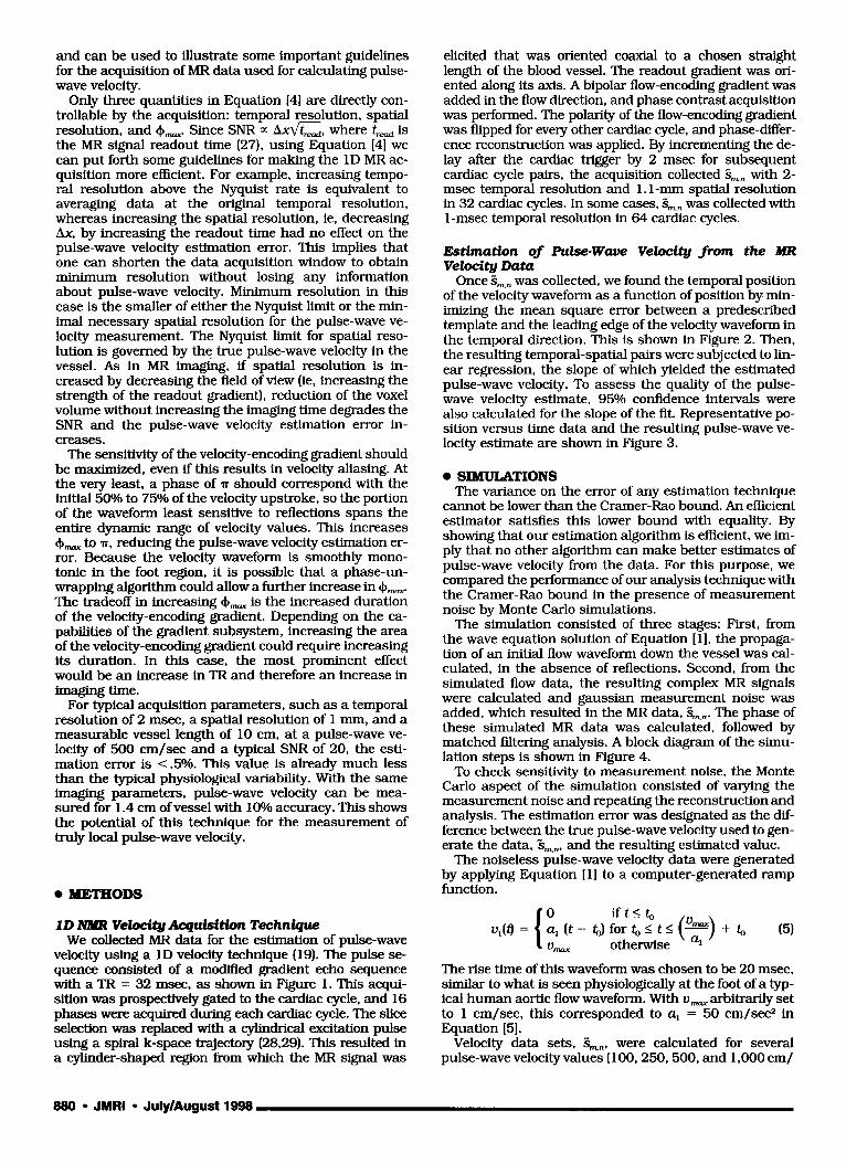
Sensitivity to Excitation-Vessel Alignment Because our MR pulse-wave velocity technique is de-

signed to make measurements in a straight length of vessel, it is important to test the sensitivity of the technique to misalignment between the velocity-encoding direction and the blood flow direction. For small angular errors, it is expected that the measured pulse-wave velocity will be c,/cos(a), where c, is the true pulse-wave velocity. With this expression, angular errors up to 8" will cause < 1% error in the pulse-wave velocity measurement. To test this experimentally, serial acquisitions were performed, with the angle of the prescribed encoding direction varied as shown in Figure 9. The resulting measurements are

shown in Figure 10 for a short section in the center of the phantom. The shorter section was used because as the angle increased, the ends of the excitation no longer intersected the phantom tube. The error in these measurements was < 1% for an angular error <5", as predicted above. GraphicaJly, a 5" error misalignment is very noticeable during the prescription process. In practice, it is not difficult to keep the errors <2", and it is typical in larger vessels to have measurable lengths of vessel that remain straight within this angular error. Considering these results, we conclude that the measurement error due to vessel-encoding alignment is neghgible.

Presence of Static Tissue and Other Flows Near the Measurement

In vivo, vessels are surrounded by other tissues, both static and moving, as well as blood flowing in neighboring vessels. The 1D MR pulse-wave velocity technique uses a cylindrical excitation pulse to isolate the MR signal to the vessel of interest. If, however, these pulses excite surrounding tissues, artifacts in the velocity data can result. To emulate static material near a vessel, we added a bag of saline next to the compliant tube in the flow phantom. The most noticeable effect was a change in amplitude and therefore in the slope of the velocity waveform as a function of position along the tube. It is known that velocities estimated by phase difference reconstruction can be un- derestimated if signal from static spins is present in the MR measurement (30). Because the matched filtering scheme is sensitive to slope and amplitude changes in the data, we normalized u ( t ) to have the same maximum velocity at each position. With this correction, the pulse- wave velocity estimate was 775 f 13 cm/sec. This value is very close to the value we measured without the saline present. If estimation was carried out without normalization of u( t ) , a large variance and bias were observed (1,015 f 359 cm/sec). Therefore, in an in vivo application of this method, extra care must be taken to eliminate signal from static tissue and/or normalization of the velocity waveform must be performed.

DISCUSSION AND CONCLUSIONS In the preceding results, we have shown that in the

presence of white noise, the 1D MR acquisition with an accompanying nonlinear parameter estimation routine approaches the Cramer-Rao lower error bound for estimation of pulse-wave velocity. This was demonstrated both through Monte Car10 simulation and with actual MR velocity data acquired in a pulsatile flow phantom. An expression for the error bound was derived by use of a 1D flow model in the absence of reflections and equations describing the MR acquisition. The resulting lower bound is dependent on several acquisition parameters of the 1D technique and the true pulse-wave velocity being measured. Because the bound was shown to be tight, it was possible to use relationships intrinsic to the error bound expression to set forth optimization guidelines for the acquisition of pulse-wave velocity data using the 1D MR technique. Because error in pulse-wave velocity measurement due to white noise in the acquisition is already very low, these guidelines can be used to make the pulse sequence more efficient. Concentration on technique development should be placed on artifact reduction.

The flow phantom used in this study modeled only some of the vascular properties encountered in vivo. The aorta is not a straight, constant-diameter, branchless homogeneous elastic tube. Because the purpose of this


n

Flgure 6. Pulsatile MR flow phantom. The pump produces a pressure pulse train that propagates down the compliant latex tube.

work was to evaluate the absolute limits of the 1D NMR pulse-wave velocity technique, the use of a very reproducible, homogeneous flow apparatus was in order. Al- though the aorta is not straight, it contains many seg- ments that can be approximated as straight, especially when regions 5 to 7 cm long are interrogated, as is typi- cally done with this technique. From the misalignment experiments, we know that a slight curvature has a negligible effect on the measured pulse-wave velocity. By the deflnition of distensibility, we know that tapering of the vessel decreases the pulse-wave velocity, but in vivo, it is often accompanied by increasing wall stiffness that results in an overall increase in wave velocity as the vessel narrows (1 7). Therefore, gradual changes as a function of position along the vessel are to be expected as a result of geometry alone. A more sudden change could indicate the presence of disease. In addition, the aorta has multiple branch points. Most of these branches are smaller than the best resolution of this technique. Branches of this size do not disturb the flow and will most likely have an insigdicant effect on the measurement. Larger branches, such as the renal arteries, however, are known reflecting sites for arterial pulse waves. Velocity measurements immediately before these branches may contain reflections that can corrupt measurements of pulse-wave velocity. Further work is necessary to assess whether accurate measurements can be made in such regions.

The phase difference reconstruction of S,, is essen- tially velocity-sampled as a function of space and time. Because this is a projection technique, the measured velocity at each position along the vessel will depend on the velocity distribution at that location. The viscosity of blood affects this distribution and has a slight effect on the measured value of pulse-wave velocity as well (31). Although the maximum velocity may vary across the vessel cross section during normal flow conditions, the ra- dial pressure gradient is extremely small (17). This implies that features in the time course of the velocity waveform, such as the foot, happen simultaneously across the vessel cross section. If, for example, the cylindrical excitation diameter is smaller than the vessel diameter, the magnitude of the measured velocity will

1 oe

1 o5

5 10'

g 10'

1 o2

73 e E a

W c

.- z! I In W

I I 0.0 5.0 10.0 15.0 20.0

Vessel Length [cm]

Figure 7. Cramer-Rao bound for unit SNR as a function of measurable vessel length. This bound is tight above a vessel length of 1 cm.

change, but the pulse-wave velocity estimated from these data should not. Furthermore, a sudden change invessel diameter, such as a local stenosis, will most likely cause nonlaminar flow conditions and severe reflections as a result of an abrupt change in vessel impedance, and this could cause errors in estimates of pulse-wave velocity.

The flow phantom also produced very reproducible pulsatile flow with cycle length variations < l%. The cardiac cycle length may not be that consistent in vivo, and the resulting velocity waveforms may vary slightly from cycle to cycle, causing errors in the measured velocity waveform. With the 1D NMR technique, the polarity of the velocity-encoding gradient is inverted during alternating cardiac cycles. Velocity data acquired in this manner have been shown to yield accurate measurements of the underlying velocity waveform (32). The interleaving method used to achieve the high time resolution with this technique, however, assumes the flow waves to be consistent over the small number of cardiac cycles required to collect the data. Because the length of the systolic in-

Volume 8 - Number 4 - JMRl * 885

100.0 ~ 90.0

80.0 - - 80.0

70.0

60.0

50.0

40.0

0 3

a - % s

30.0

20.0 0.00 0.10 0.20 0.30 0.40 0.50

Figure 8. Example pressure and velocity traces during the first 512 msec of the 1,500-msec cycle. The pressure waveform is scaled and shifted by use of the Navier-Stokes relationship to match the velocity waveform at the same position in the tube. The congruence of the curves until just past the peak suggests the existence of a discrete reflecting site downstream of the measurement point and the insensitivity of the leading edge of the waveform to reflections.

terval remains fairly constant with changes in heart rate and because we are basing our measurements on the foot of the forward-going flow wave, this technique is essen- tially making measurements of a transient phenomenon, reducing the sensitivity to fluctuations in heart rate. The high slope of the velocity waveform at the onset of flow also reduces the effect of velocity variation on detection of the waveform foot. Further development of the technique may allow collection of all velocity data in a single cardiac cycle, thereby removing any sensitivity to cardiac cycle variations.

In vivo data acquired with this technique may contain artifacts due to both prescription errors and signal from other tissues near the vessel of interest. These artifacts cause errors in estimates of pulse-wave velocity. In this work, we tested the sensitivity of the technique to these error sources. The effect of misalignment between the encoding direction and the flow direction was found to be neghgible under normal prescription conditions. The presence of static tissue near the vessel of interest does not introduce errors in the measured value of pulse-wave velocity if the velocity waveforms are normalized to the same maximum velocity before template matching is performed. The addition of extraneous signals into the MR measurement occurs because the excitation profile has a nonzero value outside the vessel. This problem can be solved through changes in the MR pulse sequence. The excitation profile can be improved, the surrounding tissue can be saturated, or the velocity encoding can be modified to reduce the contribution of signals from static tissues and flows not in the prescribed direction. These improvements, however, come at the expense of data acquisition time. When the pulse-wave velocity measurement will be used in conjunction with an interventional procedure, MR catheter antennas can be used to localize the signal and increase SNR to obtain local distensibility measurements (33).

Although the role of distensibility on the diagnosis or treatment of aortic disease has not yet been established, a technique like this that allows easy estimation of this mechanical parameter should provide a means of assess- ing its value in the clinical setting. We have demonstrated that under very controlled conditions, the 1D MR technique produces estimates of pulse-wave velocity with very low error. In addition, our analysis suggests that this

Table 2 I Summary of Pulsewave Velocity Results

Measurement Techniaue Mean k SD

fcm/secl ID MR

Pressure catheter Velocity -pressure

768+ 1.3 709 t 55 733 f 33

technique can make estimates of pulse-wave velocity with a spatial resolution not previously obtainable noninvasively. Further work is necessary to determine whether, during in vivo application, this technique can maintain the demonstrated error performance and whether that performance and the achievable spatial resolution are sdlicient to make clinically meaningful measurements. With answers to those questions, the 1D MR technique shows promise as a means of periodically and noninvasively monitoring vessel distensibility in vivo.

0 Appendix: Calculation of the Cramer-Rao Bound The MR signal for pulsatile flowing spins along an elas-

tic tube with pulse-wave velocity c, and the temporal position of the waveform foot, t,,, can be written as

where u [t - (x/c)- t,,] is the traveling velocity waveform, u,, is the maximum velocity encoded as a phase of +,,, and j = G. The actual MR data, a sampled measurement of this signal, are

rnAx 5,, = s(nAt - - C - 0 + l',"

where u is additive gaussian white noise. Ax and A t are spatial and temporal sampling periods, respectively. The data are limited by the length of the vessel being measured, L. We assume N samples of the velocity waveform in the temporal direction. The measurements are independent: thus, the joint probability density function for the acquired data, 5-, given pulse-wave velocity c and foot position t,, is

The Cramer-Rao bound for the estimation of a parameter is the inverse of the Fisher information about that parameter. In this case, we are estimating two parameters, c and t,,, and the Fisher information matrix can be written

= - I I

where Jc, 6) = -In [ p (5 1 c, t,,)] , the negative log-likelihood function reflecting the likelihood of obtaining the measurement 5, given the parameters c and t,,. * denotes the conjugate transpose.

The elements of the Fisher information matrix in Equa- tion [A41 can then be expressed as


velocity Encoding Direction

Figure 9. Misalignment between the encoding cylinder and the vessel. 8, the misalignment angle, was varied between 1" and 20".

Misalignment Angle [deg]

eigcue 10. Error in measured pulse-wave velocity as a function of alignment angle with the vessel. The dashed line shows the theoretical error, l/cos(a).

present only in the derivative of the velocity waveform, u'. If we assume that this waveform is sampled above the Ny- quist rate, allowing the summation over time to have in- finite extent will not add any more information about pulse-wave velocity. Then, applying the sampling theorem (26) in the temporal direction to show that [ x ~ ~ - m ~ ' 2 = s+" Y ' ~ (7) d ~ ] and calculating the sum in the spatial

direction (for [L/Ax >> 1, zt r n 2 - - 3Ax$). we arrive

at:

At -- L3

The other components of the Fisher information matrix can be calculated by a similar method:

Phase-difference reconstruction of the velocity data re- quires two acquisitions of the data, so the actual terms of the Fisher information matrix are twice what is calculated above. Taking this into account, to obtain the Cramer-Rao bound for our estimate of c, we use F-;, (c, or:

Substituting the above terms A7 through A10 into Equa- tion [Al l ] results in an expression for the Cramer-Rao lower bound:

Acknowledgmentcl: We thank Dr William Hunter and Dr Ogan Ocali for many helpful comments and suggestions. We also thank Dr Elias Zerhouni for his support of this project.

References 1. Noordergraaf A. Circulatory System Dynamics. Biophysics and

Bioengineering Series. San Diego, CA Academic Press, 1978. 2. Nichols WW. ORourke MF. McDonald's blood flow in arteries, 3rd

ed. Philadelphia, PA Lea & Febiger. 1990. 3. Sunagawa K, Maughan WL, Sagawa K. Stroke volume effect of

changing arterial input impedance over selected frequency ranges. Am J Physiol 1985: 248H477-H484.

4. Elzinga G, Westerhof N. Pressure and flow generated by the left

5. Mohiaddin RH, Firmin DN, Longmore DB. Age-related changes of human aortic flow wave velocity measured noninvasively by magnetic resonance imaging. J Appl Physiol 1993; 74:492-497.

6. Mohiaddin RH, Underwood SR, Bogren HG. et al. Regional aortic compliance studied by magnetic resonance imaging: the effects of age, training, and coronary artery disease. Br Heart J 1989: 62: 90-96.

m=O n=O 7. Avolio AP, Chen SG, Wang RP, Zhang CL, Li MF, ORourke MF. Effects of aging on changing arterial compliance and left ventric- ular load in a northern Chinese urban community. Circulation 1983: m50-58.

8. Demer LL. Effect of calcification on in vivo mechanical response of rabbit arteries to balloon dilation. Circulation 1991; 83:2083- 2093.

substituting the MR tion IA51,

F,,(c,td =,c U,m-O n=O I: l ~ o e e "- 186.

from Equation into Equa-

miix C ventricle against different impedances. Circ Res 1973 32:178- 1 =/Ax h ' A t -,,+s -j&Ed&--+J

d X [ -&u'(rlAt - - - (A61 C

6) Ut2 ( d t - - - d X

C

From Equation A6, we can see that the information is


9.

10.

11.

12.

13.

14.

15.

16.

17.

18.

19.

20.

21.

22.

Farrar DJ, Bond MG, Rlley WA, Sawyer JK. Anatomic correlates of aortic pulse wave velocity and carotid artery elasticity during atherosclerosis progression and regression in monkeys. Circula- tion 1991: 83:1754-1763. Franke A, Muhler EG, Klues HG, et al. Detection of abnormal aortic elastic properties in asymptomatic patients with Marfan syndrome by combined transesophageal echocardiography and acoustic quantification. Heart 1996 75307-31 1. Jeremy F W , Huang H, Hwa J, McCarron H, Hughes CF, Richards JG. Relation between age, arterial distensibility, and aortic dilation in the Marfan syndrome. Am J Cadi01 1994 74:36%373. H h t a K, ~poskiadis F, Sparks E, Bowen J, Wooley CF, Boudoulas H. The Marfan syndrome: abnormal aortic elastic properties. J Am Coll Cardiol 1991: 18:5743. Merillon JP, Motte G, Fruchaud J , Masquet C, Gourgon R Eval- uation of the elasticity and characteristic impedance of the as- cending aorta in man. Cardiovasc Res 1978 12:401406. Hansen F. Bergqvist D, Mangell P, Ryden A, Sonesson B, Lanne T. Non-invasive measurement of pulsatile vessel diameter change and elastic properties in human arteries: a methodological study. Clin Physiol 1993 13631-643. Motoi K, Morita H, Fujita N, et al. Sttfmess of human arterial wall assessed by intravasmlarulultrasound. J Cadi011995 25189-197. Drangova M, Holdsworth DW, Boyd CJ, Dunmore PJ, Roach MR. Fenster A. Elasticity and geometry measurement of vascular specimens using a high-resolution laboratory CT scanner. Physiol Meas 1993: 14:277-290. Milnor WR. Hemodynamics. Baltimore, MD: Williams & Wilkins, 1982. Lehmann ED, Parker JR, Hopkins KD, Taylor MG, Gosling RG. Validation and reproducibility of pressure corrected aortic distensibility measurements using pulse-wave-velocity Doppler ultrasound. J Biomed Eng 1993: 15:221-228. Hardy CJ, Bolster BD, McVeigh ER, Adams WJ, Zerhouni EA. A one-dimensional velocity technique for NMR measurement of aortic distensibility. Magn Reson Med 1994: 31:513-520. Bock M. Schad LR. Muller E, Lorenz WJ. pulsewave velocity measurement using a new real-time MR-method. Magn Reson Imaging 1995; 13:21-29. Urchuk SN, Plewes DB. A velocity correlation method for measuring vascular compliance using MR imaging. J Magn Reson Imaging 1995: 5:628-634. Hardy CJ. Bolster BD Jr. McVeigh ER, Iben IET, Zerhouni EA. Pencil excitation with interleaved Fourier velocity encoding:

23.

24.

25.

26.

27.

28.

29.

30.

31.

32.

33.

NMR measurement of aortic distensibility. Magn Reson Med 1996; 35814-819. Ting CT, Chang MS, Wang SP, Chiang BN, Yin FC. Regional pulse wave velocities in hypertensive and normotensive hu- mans. Cardiovasc Res 1990: 24:865-872. Wright JS, Cruickshank JK, Kontis S, Dore C, Gosling RG. Aor- tic compliance measured by non-invasive Doppler ultrasound description of a method and its reproducibility. Clin Sci 1990: 78:463-468. Lee RT, Grodzinsky AJ, Frank EH, Kamm RD. Schoen FJ. Structure-dependent dynamic mechanical behavior of fibrous caps from human atherosclerotic plaques. Circulation 1991: 83: 1764-1 770. Blahut RE. Principles and practice of information theory. Ad- dison-Wesley Series in Electrical and Computer Engineering. Reading, MA: Addison-Wesley, 1987: 262-264.300-315. McVeigh E, Atalar E. Balancing contrast, resolution, and signal- to-noise ratio in magnetic resnonance imaging. In: Bronskill MJ, Sprawls P, eds. The physics of MRI: 1992 AAPM Summer School Proceedings. American Association of Physicists in Med- icine, Woodbury, Ny: American Institute of Physics 1993; 234- 267. Pauly J, Nishimura D, Macovski A. A k-space analysis of small tip angle excitation. J Magn Reson 1989: 81:43-56. Hardy CJ, Cline HE. Broadband nuclear magnetic resonance pulses with two-dimensional spatial selectivity. J Appl Physics 1989: 66:1513-1516. Tang C, Blatter DD, Parker DL. Accuracy of phase-contrast flow measurements in the presence of partial-volume effects. J Magn Reson Imaging 1993: 3:377-385. Car0 CG, Pedley TJ, Schroter RC, Seed WA. The mechanics of the circulation. Oxford, U K Oxford University Press, 1978. Frayne R. Rutt BK. Frequency response of prospectively gated phase-contrast MR velocity measurements. J Magn Reson Im- aging 1995: 5:65-73. Bolster BD, Kraitchman DL, Ocali 0. Lesho J , Carkhuff B, Atalar E. In-vivo measurement of pulsewave velocity in the rabbit aorta using intravascular magnetic resonance. In: Proceedings of the 5th annual meeting of the International Society of Magnetic Resonance in Medicine. Berkeley, CA In- ternational Society of Magnetic Resonance in Medicine, 1997: 1878.


Accuracy of arterial pulse-wave velocity measurement using MR

Documents

Transcript of Accuracy of arterial pulse-wave velocity measurement using MR