A Dual-Pulse Repetition Frequency Scheme for Mitigating Velocity Ambiguities of the NOAA P-3...

VOLUME 17 MAY 2000J O U R N A L O F A T M O S P H E R I C A N D O C E A N I C T E C H N O L O G Y

585

A Dual-Pulse Repetition Frequency Scheme for Mitigating Velocity Ambiguities of theNOAA P-3 Airborne Doppler Radar

DAVID P. JORGENSEN AND TOM R. SHEPHERD

NOAA/National Severe Storms Laboratory, Boulder, Colorado

ALAN S. GOLDSTEIN

NOAA/Aircraft Operations Center, MacDill Air Force Base, Florida

(Manuscript received 3 May 1999, in final form 12 August 1999)

ABSTRACT

To mitigate some of the deleterious effects of the relatively small unambiguous Doppler velocity range (Nyquistinterval) of airborne X-band Doppler radars, a technique has been developed to extend this interval. Thistechnique, termed the batch-mode dual-PRF (pulse repetition frequency) technique, utilizes two batches of pulsesthat are each averaged to produce two velocity estimates at each range bin, with each batch at a different samplingrate. Comparison of the two velocity estimates produces a difference velocity that is used to dealias the secondestimate within an extended velocity range that is larger than the Nyquist velocities of either of the two originalsamples. In this implementation, the choices of the two PRFs are restricted to ratios of 3/2 or 4/3 of the lowestPRF.

Due to the spread of the input Doppler spectrum and spatial displacement from one radial to the next, however,this batch-mode technique can produce processor velocity dealiasing mistakes, particularly in high wind shearenvironments. For PRFs less than about 2000 s21, processor mistakes can easily exceed 10% of all data points.With higher PRFs using the 3/2 ratio, the number of processor mistakes decreases to a few percent of the totalnumber of samples even when observing strong convective storms and mesoscale convective systems. Testresults from convective storm environments are shown from the airborne Doppler radar operated on the NationalOceanic and Atmospheric Administration’s P-3 instrumented aircraft for a variety of base PRFs and ratios toshow the utility of this technique.

1. Introduction

Conventional pulse-Doppler radars transmit a seriesof equally spaced pulses, which produce a return signalfrom the scatterers of interest that have their electro-magnetic frequency phase-shifted in proportion to therelative velocity between the radar antenna and target.The maximum radial velocity that a pulse-Doppler radarcan detect unambiguously is given by the velocity,which just produces a phase shift of 61808. This ve-locity is termed the Nyquist velocity (Vn) and is ex-pressed as (Battan 1973):

lPRFV 5 6 , (1)n 4

where l is the radar wavelength in meters and PRF isthe pulse repetition frequency in inverse seconds. For

Corresponding author address: Dr. David P. Jorgensen, NOAA/NSSL/Mesoscale Research and Applications Division—Boulder,Mail Code N/C/MRD, 325 Broadway, Boulder, CO 80303-3328.E-mail: [email protected]

the airborne X-band (l 5 0.0322 m) Doppler radar op-erated on the P-3 aircraft operated by the National Oce-anic and Atmospheric Administration (NOAA), Vn is612.88 m s21 for a nominal PRF of 1600 s21. Othercharacteristics of the P-3 radar are shown in Table 1.The maximum PRF of the P-3 radar transmitter is 3200s21, for which Vn is 625.76 m s21.

The proper interpretation of airborne Doppler radardata (Jorgensen et al. 1996) depends on accurate place-ment of aliased velocities into their proper interval (de-aliasing), usually by a combination of automated al-gorithms (e.g., Bargen and Brown 1980) and manualinspection (Oye et al. 1995). For extremely high shearsituations, for example, convective storms and regionswithin mesoscale convective systems (MCSs), this taskcan be onerous and extremely time consuming. For ex-ample, an experienced Doppler radar analyst (C. L. Zie-gler 1998, personal communication) took about 3.5man-months to completely dealias just seven passes bya tornadic supercell thunderstorm observed during theVerification of the Origins of Rotation in ThunderstormsExperiment (Ziegler et al. 1998). In some cases of veryhighly sheared storms, it is not even possible to reliably

586 VOLUME 17J O U R N A L O F A T M O S P H E R I C A N D O C E A N I C T E C H N O L O G Y

TABLE 1. Characteristics of the NOAA P-3 vertical scanningDoppler radar.

Parameter Tail radar

Scanning method Vertical about the aircraft’s lon-gitudinal axis; fore/aft alternatesweep methodology.

Wavelength 3.22 cm (X band)

BeamwidthSteerable antenna

HorizontalVertical

1.3581.908

CRPE flat plate antennaHorizontalVertical

Aft: 2.078, fore: 2.048Aft: 2.108, fore: 2.108

Polarization (along sweep axis)Steerable antennaCRPE flat plate antenna

Linear verticalLinear horizontal

SidelobesSteerable antenna

HorizontalVertical

223.0 dB223.0 dB

CRPE flat plate antennaHorizontalVertical

Aft: 257.6 dB, fore: 255.6 dBAft: 241.5 dB, fore: 241.8 dB

GainSteerable antennaCRPE flat plate antenna

40.0 dBAft: 34.85 dB, fore: 35.9 dB

Antenna rotation rate Variable up to 10 rpm (608 s21)

Fore/aft TiltSteerable antenna Variable up to 6258CRPE flat plate antenna Aft: 219.488, fore: 19.258

Pulse repetition frequency Variable, 1600 s21–3200 s21

Dual-PRF ratios 3/2 and 4/3Pulses averaged per radial Variable, 32 typicalPulse width 0.5 ms, 0.375 ms, 0.25 msGate length 150 m

FIG. 1. Schematic depiction of the batch-mode dual-PRF techniqueas implemented on the NOAA P-3 vertically scanning tail-mountedradar. Successive radials of Doppler velocity data are collected atdifferent sampling rates (PRFs). The angular displacement betweensuccessive radials is shown by Du9. The boxes along each radialrepresent individual range gates.

dealias all the folded velocities with a high degree ofconfidence. An improvement to the NOAA P-3 Dopplerradar to extend the Nyquist velocity is needed becausethe aircraft is being increasingly utilized to investigatea variety of convective storms, hurricane, and mesoscalephenomena (e.g., Jorgensen et al. 1997). A simple wayto extend the Nyquist velocity is to increase the PRFof the radar [Eq. (1)]. Unfortunately, the maximum un-ambiguous range (Rmax) of pulse-Doppler radars islinked to the Nyquist velocity through the Doppler am-biguity relationship

clR V 5 , (2)max n 8

where c is the speed of light. For the NOAA P-3 Dopplerradar, Eq. (2) shows that increasing Vn to an acceptablevalue for the study of severe convective storms, hur-ricanes, and MCSs (i.e., .|40| m s21) would result inan unacceptably low maximum range (;30 km). A shortmaximum range would also increase the likelihood ofrange-folded echoes (i.e., targets beyond Rmax) contam-

inating the data at ranges less than Rmax, requiring furthermanual editing.

To mitigate some of the problems caused by the con-flicting desire for a relatively long unambiguous max-imum range and simultaneous large Nyquist velocity,an alternative method for extending the Nyquist velocityinterval is proposed that is based on comparison of twovelocity estimates made at different PRFs. Because theradar sends out pulse streams at alternate PRFs, themethod is termed the ‘‘batch-mode dual-PRF’’ ap-proach. Figure 1 illustrates the concept. In this approach,the first radial of data is used to ‘‘dealias’’ the secondradial by a gate-to-gate comparison of respective ve-locities.

Implementation of this dual-PRF technique on theNOAA P-3 radar system was begun in late 1997. As aninitial test, modifications to the existing signal process-ing software were made to allow for the collection ofalternating radials of data at two PRFs. The two PRFsare constrained to be at ratios of 4/3 or 3/2 of the lowestPRF. Each velocity estimate consists of an integrationof a number of pulses, usually 32, but subject to a max-imum PRF of only 1600 s21. Subsequent modificationsto the transmitter/receiver allowed for a maximum PRFof 3200 s21. The current signal processing hardwaredoes not allow for true ‘‘interlaced’’ sampling (termed‘‘staggered’’ PRF sampling) where both PRF samplesare collected nearly simultaneously by alternating pulsesat different rates. This approach is employed on theELDORA (Electra Doppler radar) operated by the Na-tional Center for Atmospheric Research. Rather a

MAY 2000 587J O R G E N S E N E T A L .

FIG. 2. (a) Estimated measured Doppler radial velocity vs truevelocity for two radials (B1 and B2) of monotonically increasing truevelocity using Nyquist velocities V1 (thick black line) and V2 (thingray line), where V1/V2 5 4/3. (b) Estimated gate-to-gate velocitydifferences vs true velocity. The difference pattern repeats outsidethe interval 6Vmax, which is the extended Nyquist velocity after pro-cessor dealiasing.

‘‘batch-mode’’ approach had to be used, where succes-sive radials of data are collected at alternating PRFs.

Because the antenna makes a vertical scan about thelongitudinal axis parallel to the aircraft’s fuselage, usu-ally at 608 s21, there is some spatial offset between thepaired velocity estimates. If the wind shear in the azi-muthal direction (i.e., direction of rotation that wouldbe mainly vertical wind shear) is large enough, or if thespread of the Doppler spectrum is large enough, thepossibility exists that the signal processor will assigndata values to the incorrect difference interval when thedealiasing occurs. These processor ‘‘mistakes,’’ andpossible mitigation, are explored in section 4. Futureenhancements to the P-3 Doppler radar system couldinvolve the development of new signal processing hard-ware to allow for a staggered pulsing scheme that wouldmitigate the effects of antenna rotation on unfoldingmistakes. A brief history and the basic methodology ofthe dual-PRF technique is given in section 2. Specificexamples are shown in section 3. In section 5 we presentconcluding remarks.

2. The dual-PRF technique

a. History

The dual-PRF approach to mitigating Doppler radarvelocity ambiguities was first used in military appli-cations of detecting moving targets (i.e., airplanes) inthe presence of ground clutter (Natheson 1969; Perlman1958). The technique was extended to weather radarapplications by Sirmans et al. (1976). Loew and Walther(1995) first implemented the technique to airborneweather radars for use by the ELDORA radar. Theirapproach utilized staggered pulse sampling rather thanthe dual-PRF processing used on the NOAA P-3. TheELDORA approach has the distinct advantage of nearlysimultaneous sampling of both velocity estimates andwas highly successful in extending the Nyquist velocityin severe convective storm environments, as shown bythe observations in Wakimoto et al. (1996).

b. Methodology

If a pulse-Doppler radar samples approximately thesame region of a weather target with two separate pulsetrains (PRF1 and PRF2) the respective Nyquist velocities(V1 and V2), will cause the two velocity estimates (B1

and B2) to be different if the true velocity is beyond6V2. If the statistical fluctuations (Doppler variance) inthe mean velocity estimate are small compared to theNyquist velocity differences, the difference (B1 2 B2)can be used to reliably dealias either estimate within anextended velocity range that is larger than either V1 orV2. This extended Nyquist velocity, Vmax, can be shownto be (Doviak and Zrnic 1984)

lV 5 6 , (3)max 4(T 2 T )2 1

where T1 and T2 are the times between each pulse(1/PRF1 and 1/PRF2, respectively) of the paired sam-ples. Equation (3) shows that the smaller the differencebetween the interpulse periods, the larger the extendedNyquist velocity. However, because the variance of themean estimate is inversely proportional to the differenceT2 2 T1 (Doviak and Zrnic 1984), the number of pro-cessor mistakes increases as T2 2 T1 decreases. If thevariance of the mean velocity estimates is large or ifthe region sampled by the two beam volumes has asignificantly different radial velocity due to wind shear,velocity dealiasing errors can occur.

In the implementation of the dual-PRF technique, itis convenient to restrict the ratio V1/V2 5 C1/C2, whereC1 and C2 are unequal integers larger than 1, and C1 .C2. The two PRFs are related to the ratio C1/C2 by Eq.(1) as PRF1/PRF2 5 C1/C2. For the P-3 Doppler radarimplementation, two ratios are used: 3/2 and 4/3. Testsusing these ratios are shown in section 3.

An illustration of the dual-PRF technique is shownin Fig. 2 for the case of a 4/3 ratio. Figure 2a showswhat a Doppler radar would measure for two radialvelocity estimates, B1 and B2, at two different PRFsrelated by PRF1/PRF2 5 C1/C2 5 4/3, for a monoton-ically increasing true radial velocity. The expected dif-ference between the two estimates is confined to 2C2

1 1 intervals (seven for the example shown in Fig. 2b).These intervals are evenly spaced over the range 62V2

with a spacing of 2V2/C2. Outside the extended Nyquistinterval 6Vmax 5 C1V2 5 C2V1 the pattern of differencesbetween the paired velocity samples repeats. Thus, with-in this extended Nyquist interval given by 6Vmax, it ispossible to dealias both mean velocity estimates to find


TABLE 2. Methodology for dealiasing of dual-PRF data using a C1/C2 ratio equal to PRF1/PRF2. Note that a ratio of 3/2 would only usethe middle five intervals. Here V1 and V2 are the Nyquist intervals of the two radials of data, B1 and B2, respectively. The expected gate-to-gate velocity differences, DB 5 B1 2 B2, fall into evenly spaced intervals given by the second column. The procedure for adjusting eachvelocity estimate to make them consistent is tabulated in the columns labeled B1 and B2 adjustment.

Velocity intervalExpected difference

velocity DB 5 B1 2 B2

B1

adjustmentB2

adjustment

23V1 , v , 23V2

23V2 , v , 2V1

2V1 , v , 2V2

2V2 , v , V2

V2 , v , V1

V1 , v , 3V2

3V2 , v , 3V1

22(2V2 2 V1)22(V2 2 V1)22V2

02V2

2(V2 2 V1)2(2V2 2 V1)

Subtract 2V1

Subtract 2V1

000Add 2V1

Add 2V1

Subtract 4V2

Subtract 2V2

Subtract 2V2

0Add 2V2

Add 2V2

Add 4V2

the true mean velocity based strictly on the differencesbetween the two estimates. Table 2 details the differenceestimates and dealiasing procedures for a choice of C2

# 3. In general, larger values of PRF1 and C2 producelarger extended Nyquist (C2V1) velocities. However,larger values of C2 would generally produce more pro-cessor dealiasing mistakes because the difference inspacing (2V2/C2) becomes progressively smaller and isultimately comparable to the statistical fluctuations ofthe estimated mean velocity. Table 2 can easily be ex-tended for any choice of C2.

For the P-3 Doppler radar, the methodology for ex-tending the Nyquist interval consists of alternately trans-mitting and integrating N pulses at PRF1 to produce oneradial of data followed by N pulses at PRF2. The Npulses (typically N 5 32, to reduce the expected stan-dard deviation of the Doppler spectrum to ;2 m s21;Jorgensen et al. 1983) are averaged to yield a reflectivityand radial velocity estimate at each of 512 gates, spaced150 m apart. Values along the two radials are subtracted,gate by gate, to produce a set of difference velocities.This difference velocity is used to adjust the secondvelocity estimate, according to Table 2, so that the twoestimates are consistent. For example, if the differencevelocity was within the range 2(2V1 2 V2) 6 V2/C2,then the second velocity estimate would have 2V2 addedto it. The first velocity estimate could also be adjusted(by having 2V1 added to it) to make it consistent withthe second estimate, but that is not done in this imple-mentation of the technique. The process continues withthe third batch of pulses at PRF1 being dealiased by theprevious estimate. Other difference intervals and un-folding rules beyond the scope of Table 2 can easily bederived for any choice of PRF pairs (i.e., C1 and C2).

3. Examples

Two test flights of the NOAA P-3 were performed toevaluate the dual-PRF technique. The first test flightoccurred on 31 October 1997, near convective stormsassociated with an advancing cold front in the Gulf ofMexico, and involved a maximum PRF of 1600 s21.During May 1998, the National Severe Storms Labo-ratory (NSSL) conducted an investigation called the

MCS Electrification and Polarimetric Radar Study(MEaPRS), which used the P-3 to fly patterns in andaround MCSs that were also being probed by ground-based polarimetric radar and balloons bearing electricfield meters. The first flight mission in MEaPRS in-volved an attempt to evaluate the optimum choices fora dual-PRF configuration in order to investigate severeweather and MCSs (i.e., the maximum PRF and ratioof PRFs). The choices that were evaluated are listed inTable 3.

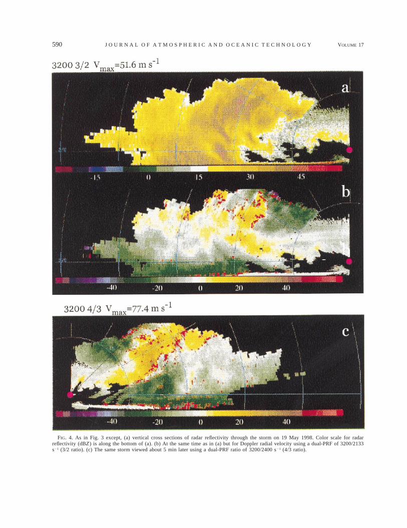
An example of raw radial velocity from a sweepthrough the leading edge of an MCS observed on 19May 1998 is shown in Fig. 3. In Fig. 3a a unispacedPRF of 1600 s21 shows many ‘‘folds’’ in the velocitydata (i.e., boundaries in the velocity field where thevelocity abruptly changes from 1Vn to 2Vn or viceversa), which would necessitate manual correction be-fore proper interpretation. Figure 3b shows an examplesweep from another pass but using dual PRFs of 2133/1422 s21 (a 3/2 ratio), in which all of the real folds havebeen eliminated because the extended Nyquist interval(34.4 m s 21) is larger than any real radial velocity. Theexceptions are data points flagged as red, which arevelocities greater than |22| m s21 from a seven-gate run-ning mean. These ‘‘bad values’’ represent processor de-aliasing mistakes. The cause of these dealiasing mis-takes is explored more fully in section 4. These mistakestend to occur more frequently in regions where there islarge azimuthal (mainly vertical) wind shear, (e.g., closeto the ground) or in regions of strong radial conver-gence, (e.g., near the edges of the sloped yellow zonein Fig. 3b, which is likely a region of strong updraft).Figure 3c shows data from a pass about 11 min afterthe middle panel but using a PRF ratio of 2133/1600s21 (4/3 ratio). Many more processor dealiasing mistakesare seen in this second pass, most likely because thedifference interval is smaller (Table 3).

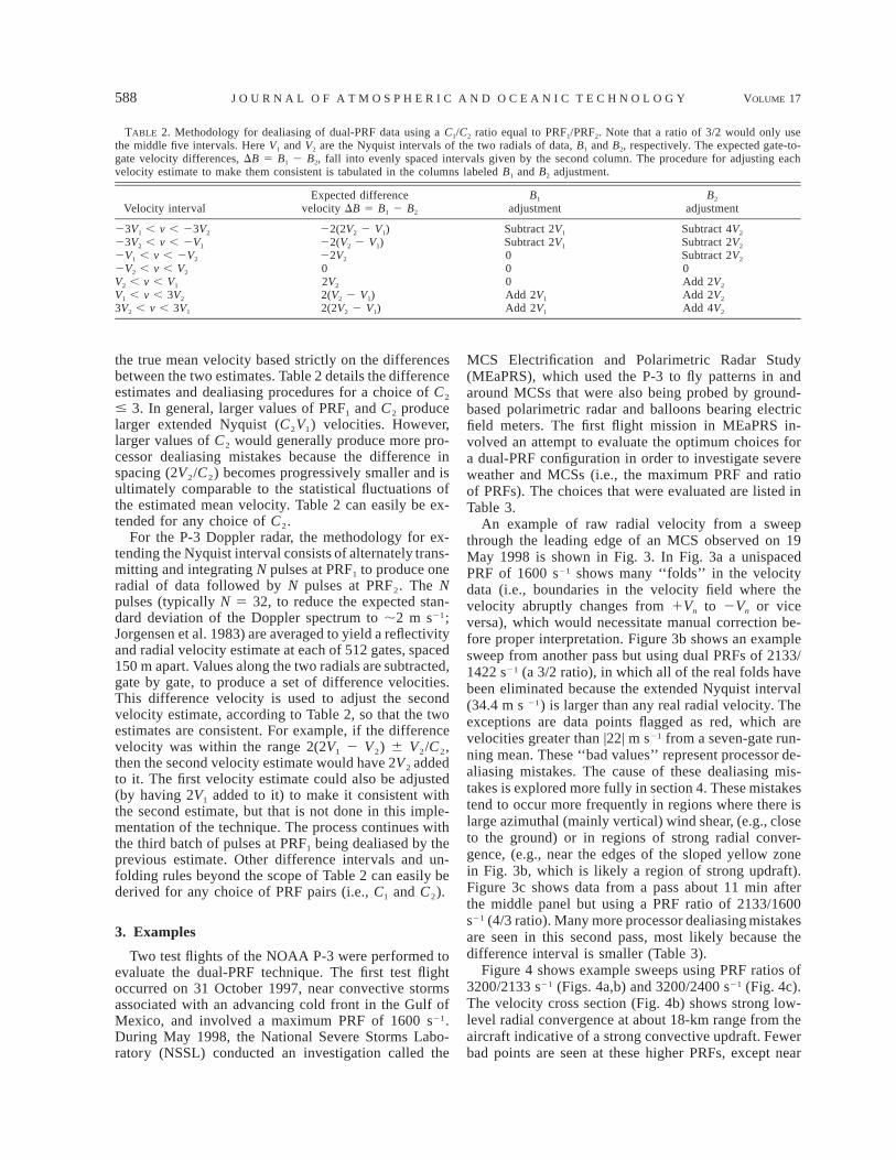
Figure 4 shows example sweeps using PRF ratios of3200/2133 s21 (Figs. 4a,b) and 3200/2400 s21 (Fig. 4c).The velocity cross section (Fig. 4b) shows strong low-level radial convergence at about 18-km range from theaircraft indicative of a strong convective updraft. Fewerbad points are seen at these higher PRFs, except near


FIG. 3. Vertical cross sections of Doppler radial velocity through the leading edge of the MEaPRS MCS on 19 May 1998: (a) A unispacedPRF of 1600 s21, aliased velocities are indicated as the boundaries between yellow and green contours; (b) a dual-PRF of 2133/1422 s21

(3/2 ratio); and (c) a dual PRF of 2133/1600 s21 (4/3 ratio). Color scale for radial velocity (m s21) is along the bottom of each panel. Redpixels correspond to radial velocities that exceed |22 m s21| from an eight-gate running mean. Aircraft location on each panel is indicatedby the magenta dot. Range rings are every 10 km.


FIG. 4. As in Fig. 3 except, (a) vertical cross sections of radar reflectivity through the storm on 19 May 1998. Color scale for radarreflectivity (dBZ ) is along the bottom of (a). (b) At the same time as in (a) but for Doppler radial velocity using a dual-PRF of 3200/2133s21 (3/2 ratio). (c) The same storm viewed about 5 min later using a dual-PRF ratio of 3200/2400 s21 (4/3 ratio).


TABLE 3. Choices for PRF and PRF ratio. Here, V1 and V2 are the two Nyquist intervals, Rmax and Vmax the maximum unambiguous rangeand dual-PRF extended Nyquist velocity, respectively, and DV the interval width. Processor dealiasing mistake percentages are from repeatedP-3 flight legs ahead of a mesoscale convective line on 19 May 1998 in central Kansas, except for data with PRF1 5 1600 which werederived from data collected on 31 Oct 1997 of tropical convective storms along an active cold front in the Gulf of Mexico.

PRF1/PRF2 C1/C2

V1/V2

(m s21)

Rmax

(km)(highest

PRF)Vmax

(m s21)

DV5(2V1/C1) 5(2V2/C2) 52(V1 - V2)

(m s21)

Percentdealiasingmistakes

1600/10671600/12002133/14222133/16003200/21333200/2400

3/24/33/24/33/24/3

12.9/8.612.9/9.717.2/11.517.2/12.925.8/17.225.8/19.3

93.793.770.370.346.846.8

25.838.734.451.651.677.4

8.66.4

11.58.6

17.212.8

5.56*10.45*9.51

14.863.235.56

* Obtained from Gulf of Mexico convection.

FIG. 5. Probability density function of expected velocity differencesfor a PRF ratio of 4/3 for the first interval centered around DB50 inFig. 1. The shaded area under the curve beyond DB . 6V1/4 rep-resents the fraction of the sampled population that would be placedin the wrong Nyquist interval. The spectrum width (standard devi-ation) of the sampled velocity distribution is shown by ss. In general,the interval width is 2V2/C2 5 2V1/C1.

the ground, near echo top, and along the edges of thestrong updraft.

The percentage of bad values for each pass is shownin Table 3. The percentage of bad values, in general,increases for lower PRFs and smaller difference inter-vals. These dealiasing mistakes, fortunately, can easilybe detected and deleted by comparison with their neigh-bor data points since they are about two Nyquist inter-vals removed from their correct velocity (Table 2). How-ever, synthesis of pseudo-dual-Doppler wind fields fromthese passes (not shown) reveal that dealiasing mistakepercentages greater than about 10%–15% could signif-icantly affect the coverage of the derived dual-Dopplerwind fields because of insufficient data points beinginterpolated to Cartesian grid points. Also, since the badvalues occur most frequently in regions of high shear,

selectively deleting these points has a noticeable effecton the strength of updrafts and downdrafts, which arecomputed from vertical integration of horizontal diver-gence. Dealiasing mistake percentages from the passesusing PRF1 5 1600 s21 (Gulf of Mexico convectivestorms) are probably too low in comparison to thoseobtained during MEaPRS owing to differing shear inthese two environments. Dual-PRF data were not col-lected during MEaPRS at PRF1 5 1600 s21, but had itbeen, the dealiasing mistake percentages would mostlikely be much greater than the 5%–10% shown in Table3 because of the higher inherent wind shear in MEaPRScompared to tropical convection.

4. Cause of processor dealiasing mistakes

Processor dealiasing mistakes are caused by the dif-ference velocity being assigned to the wrong differenceinterval, with the resultant correction being improperlyoffset by the amount shown in the last two columns ofTable 2. Unfortunately, the P-3 radar data system doesnot currently record which PRF was used to constructeach radial, so the processor dealiasing mistakes cannotbe readily corrected in postflight analysis. The fact thatthese dealiasing mistakes occur more frequently in re-gions of larger shear implies that the error rate is pro-portional to the Doppler spectrum width. With this as-sumption, how a processor mistake can be made isshown schematically in Fig. 5. Figure 5 shows a 4/3ratio assuming that the difference estimates conform toa Gaussian distribution. The probability of an error incategorization (i.e., the probability that the processorplaces the estimate in the wrong Nyquist interval) is theprobability that the difference estimate deviates from itsexpected value by more than one-half of the differenceinterval, assuming the case of a symmetric differenceprobability density. The Doppler spectrum can be ap-proximated by a Gaussian function independent of thevelocity spectral density if the estimate contains a rel-atively large number of independent samples, and thesignal-to-noise ratio is small (Doviak and Zrnic 1984).


FIG. 6. Velocity dealiasing error rate as a fraction of the totalnumber of samples for a Gaussian distribution of difference estimates.Abscissa is one-half the difference interval normalized by the Dopplerspectrum width times 2. The solid line is for zero offset, the dottedÏline for an offset of 0.5 normalized difference velocity, and thedashed–dot line for an offset of 1.0 normalized difference velocity.

Since the distributions of radial velocity values from asufficiently large number of paired estimates are ap-parently Gaussian, the difference velocity, being a linearoperator, is also Gaussian but with a unique standarddeviation defined by

var[DB] 5 1 2 2r12s1s2,2 2s s1 2 (4)

where s1 and s2 are the standard deviations of two meanvelocity estimates and r12 is the correlation between theestimates. Sirmans et al. (1976) has shown, for the stag-gered PRF scheme, that r12 effectively goes to 0 fornormalized spectrum widths greater than about 0.20. Forthe dual-PRF scheme, r12 is also small because the timeit takes the radar to collect both samples (64 samplesor 0.0233 s at 3200/2400 s21) is much longer than thetypical decorrelation time of the scatterers (;0.0017 s).Hence, for relatively narrow spectra, Eq. (4) shows thatthe probability density function for the expected veloc-ity differences has a standard deviation of 2ss (s1 5Ïs2 5 ss, where ss is the Doppler input spectrum width,estimated to be about 2 m s21 (Jorgensen et al. 1983)for N 5 32. The likelihood of processor dealiasing er-rors, represented by the shaded regions in Fig. 5, is theprobability P(x) of a difference estimate being outsidethe region x 5 6(V1 2 V2) and can be estimated as thearea under the standard normal curve:

x 21 2(x 1 m)P(x) 5 1 2 exp dx, (5)E [ ]2Ï2p 2x

where m is an offset representing a bias between thetwo radials. Figure 6 is a plot of Eq. (5) for variousvalues of m. The dealiasing error rate (or fraction of thetotal estimates expected to be placed in the wrong Ny-quist interval) for m 5 0 (no bias between radials) isshown as the curve labeled ‘‘0’’ in Fig. 6. The curvelabeled ‘‘0’’ expresses the dealiasing error rate in termsof the difference interval normalized by the spectrumwidth. Note that the error rate does not go below a fewpercent until the normalized velocity difference exceedsabout 2.5. For the P-3 radar, ss is about 2 m s21, so thedifference between the Nyquist velocities of the twoestimates needs to be larger than about 7.1 m s21 toreduce the expected processor dealiasing errors to anacceptable level for even a nonrotating antenna col-lecting perfectly collocated samples. In practice, thePRFs that were evaluated produce differences that areup to 17.2 m s21 (column labeled DV of Table 3), whichwould reduce the number of dealiasing mistakes to afew percent, in accordance with what was observed inthe P-3 data (column labeled ‘‘dealiasing mistakes’’ ofTable 3). It is also seen in Fig. 6 that the smaller thedifference interval or the greater the spread of the Dopp-ler spectrum ss, the higher the probability of making aprocessor dealiasing error, which is also reflected in thepercentage of bad value statistics shown in Table 3.

Wind shear (in the azimuthal direction) also increasesprocessor dealiasing mistakes since the two radials are

not strictly collocated in space. If there are biases in themeans of the B1 and B2 distributions, then DB will shiftaway from zero in Fig. 5, resulting in more area underthe P(x) curve being beyond the half interval region.Rather than collocated, the two radials making up eachdual-PRF pair are displaced about the axis of rotationby an amount

NDu 5 v, (6)

PRF

where v is the antenna rotation rate. Clearly, Eq. (6)shows that slowing the rotation rate for a given N andPRF will reduce the impact of wind shear on the numberof processor dealiasing mistakes since the two adjacentradials will be physically closer (in the sweep direction).Unfortunately, the horizontal or along-track data spac-ing of the pseudo-dual-Doppler derived winds is in-versely proportional to the antenna rotation rate (Jor-gensen et al. 1996), so v is usually chosen to be as largeas possible (608 s21) to produce Cartesian wind vectorson closely spaced grids (;1 km). Therefore, minimizingthe angular displacement between two adjacent radialsmeans transmitting as high a PRF as possible since itis also desirable to integrate a large number of pulsesto keep ss small. One estimate for the largest desirablespacing between adjacent radials is half of the verticalhalf-power beamwidth of the antenna (0.858). For N 532, Du 5 0.858, and v 5 608 s21, the lowest PRF from


Eq. (6) should be greater than about 2000 s21 so thetwo radials are collected within a vertical beamwidth.If a 4/3 ratio is used for the higher PRF, it would be2667, which limits the maximum range by Eq. (1) toabout 55 km—a tolerable limitation for mapping windfields within convective storms, MCSs, and hurricanes.

An estimate of the effects of wind shear on processordealiasing mistakes is seen in the two curves in Fig. 6labeled ‘‘0.5’’ and ‘‘1.0.’’ These two curves representthe effect of offsets between the two radials of one-halfand one normalized difference interval, respectively.For example, for a 3/2 ratio using PRF1 5 3200 s21 andss 5 2 m s21, the two curves represent biases betweensequential radials of 1.5 and 3.0 m s21, respectively.Thus, wind shear represents a serious limitation to thisparticular implementation of the dual-PRF technique.For the above example, Fig. 6 reveals that if the windshear produced a 3 m s21 bias between sequential ra-dials, the effect on the dual-PRF dealiasing processwould be to increase the dealiasing mistakes by a factorof 5 over no bias for comparable normalized differencevelocities. Slowing the rotation rate, changing the ratio,increasing the base PRF, or decreasing the number ofpulses integrated reduces the angular separation betweenradials. Each of these choices has impacts on other as-pects of data gathering including the possibility of in-creasing the number of processor dealiasing errors.

5. Conclusions

Optimal operation of the P-3 airborne Doppler radarsystem (in terms of data quality and minimal postflightanalysis time) involves trade-offs between Nyquist ve-locity, maximum range, antenna rotation rate, and ac-curacy of the estimated Doppler velocity. Frequentlythese choices are in conflict with each other (e.g., greatermaximum range and larger Nyquist interval), which lim-its the utility of the airborne radar system to probe thestructure of severe convective weather, MCSs, and hur-ricanes. A dual-PRF technique is presented that extendsthe Nyquist velocity interval without seriously compro-mising the maximum range. In this technique, Dopplervelocity estimates along each of two sequential radialsare made at different sampling rates that are C1/C2 ratiosof each other (C1 and C2 are unequal integers greaterthan 1, with C1 . C2), which produces different Nyquistvelocities (V1 and V2). The two velocity estimates aresubtracted to produce a velocity difference, which isused to determine the true velocity within a larger ex-tended Nyquist interval of 2C1V2 5 2C2V1 because thevelocity differences occur only at prescribed intervals.

The dual-PRF technique was evaluated using datacollected by the P-3 flying near tropical convection anda Midwest U.S. mesoscale convective system. Sequen-tial passes using various paired sets of PRFs reveal thedisadvantages of low PRFs and PRF ratios above 3/2.Processor dealiasing errors occur because the largerDoppler spectrum width and inter-radial biases in high

shear regions cause the difference estimate to be placedin the wrong category, which is unrecoverable in thecurrent P-3 Doppler radar signal processor design. For-tunately, the dealiasing mistakes do not seriously com-promise pseudo-dual-Doppler wind field construction aslong as they are less than about 5% of the total numberof samples because the errors can be easily removed byan automated procedure. If the percentage of dealiasingmistakes is less than 5%, the resulting wind field is notdegraded because of the high degree of oversamplingin the radial direction relative to the Cartesian grid sizeon which the winds are calculated (150-m radial spacingversus typically 1-km Cartesian grid spacing).

For the P-3 radar, this study indicates that weathersystems that contain high wind shear demand a highbase PRF (.;2000 s21) to keep the processor unfoldingmistakes to less than about 5% or less of the total num-ber of samples. The reduction in processor dealiasingmistakes at high PRFs results from both narrowing theangle swept by the antenna during collection of adjacentradials at alternating PRF, and enlarging the velocitydifference interval relative to the Doppler spectrumwidth. Our test results indicate that a base PRF of 3200s21, with either a 3/2 or 4/3 ratio is acceptable for thestudy of convective storms. Using these values of PRFand ratio results in an extended Nyquist velocity intervalof 51.6 and 77.4 m s21, respectively, yet allows for amaximum range of approximately 46 km, which is nota serious range limitation for the study of severe con-vective storms, MCSs, or hurricanes.

Future enhancements to the P-3 airborne Doppler ra-dar may include the development of a true interlaced(i.e., staggered) pulsing scheme. With this approach asignificant source of processor dealiasing errors wouldbe eliminated (i.e., those errors arising due to antennamotion between adjacent radials) since the two estimatesare obtained simultaneously. The diminished number ofdealiasing errors provided by the staggered PRF schemeover the dual-PRF scheme would be offset somewhatby an increased number of errors because only half thenumber of pulses would be used to construct each ve-locity estimate, resulting in an increased Doppler spec-tral width (Fig. 6). The final dealiased velocity providedby the staggered PRF scheme would be an average ofthe two original samples, so the accuracy of the estimatewould be identical to that obtained by the dual-PRFapproach.

Last, for each meteorological situation, the advantag-es of automated velocity dealiasing should be weighedagainst the disadvantages of processor mistakes and theanalyst’s time required to remove them. For example,in mapping the velocities of extensive stratiform rainregions, often seen in hurricanes and some MCSs, alarge maximum range is usually more important than ahigh Nyquist velocity since the velocity data can usuallybe successfully dealiased using automated radial con-tinuity algorithms (e.g., Bargen and Brown 1980) inspite of relatively high wind velocities. In those situa-


tions, the airborne Doppler scientist could elect not touse the dual-PRF approach since the processor dealias-ing mistakes would likely be excessive because of thelow PRF used to achieve the long range.

Acknowledgments. We wish to acknowledge the ef-forts of the NOAA P-3 flight crews from the AircraftOperations Center in Tampa, Florida, who executed theflight patterns used in this study. Without their dedi-cation and enthusiastic support of our scientific en-deavors the collection of airborne Doppler radar datanear hazardous weather conditions would not be pos-sible. Robert Hueftle was instrumental in developmentof the Doppler wind synthesis and display software.Editing of the radar data was accomplished with theNCAR/SOLO software package provided by Dick Oyeof NCAR/ATD. Jim Barr, Jorge Delgado, and JimDuGranrut of NOAA/AOC modified the P-3 Dopplerradar transmitter/receiver to allow the maximum PRFto be extended to 3200 s21, following initial work byTerry Schricker beginning in 1994. Jim Barr collectedthe first dual-PRF data on 31 October 1997. Brad Smulland Wen-Chau Lee provided many suggestions for im-provements to the manuscript.

REFERENCES

Bargan, D. W., and R. C. Brown, 1980: Interactive radar velocityunfolding. Proc. 19th Conf. on Radar Meteorology, Miami, FL,Amer. Meteor. Soc., 278–283.

Battan, L. J., 1973: Radar Observations of the Atmosphere. Universityof Chicago Press, 324 pp.

Doviak, R. J., and D. S. Zrnic, 1984: Doppler Radar and WeatherObservations. Academic Press, 458 pp.

Jorgensen, D. P., P. H. Hildebrand, and C. L. Frush, 1983: Feasibilitytest of an airborne pulse-Doppler meteorological radar. J. Cli-mate Appl. Meteor., 22, 744–757., T. Matejka, and J. D. DuGranrut, 1996: Multi-beam techniquesfor deriving wind fields from airborne Doppler radars. J. Meteor.Atmos. Phys., 59, 83–104., M. A. LeMone, and S. B. Trier, 1997: Structure and evolutionof the 22 February 1993 TOGA COARE squall line: Aircraftobservations of precipitation, circulation, and surface energyfluxes. J. Atmos. Sci., 54, 1961–1985.

Loew, E., and C. Walther, 1995: Engineering analysis of dual phaseinterval radar data obtained by the ELDORA radar. Preprints,27th Conf. on Radar Meteorology, Vail, CO, Amer. Meteor. Soc.,710–712.

Nathanson, F. E., 1969: Radar Design Principals. McGraw-Hill, 626pp.

Oye, R., C. Mueller, and S. Smith, 1995: Software for radar trans-lation, visualization, editing, and interpolation. Preprints, 27thConf. on Radar Meteorology, Vail, CO, Amer. Meteor. Soc.,359–361.

Perlman, S. E., 1958: Staggered repetition rate fills radar blind spots.Electronics, 31, 82–85.

Sirmans, D., D. Zrnic, and B. Bumgarner, 1976: Extension of max-imum unambiguous Doppler velocity by use of two samplingrates. Proc. 17th Conf. on Radar Meteorology, Seattle, WA,Amer. Meteor. Soc., 23–28.

Wakimoto, R. M., W.-C. Lee, H. B. Bluestein, C.-H. Liu, and P. H.Hildebrand, 1996: ELDORA observations during VORTEX 95.Bull. Amer. Meteor. Soc., 77, 1465–1481.

Ziegler, C. L., T. R. Shepherd, E. N. Rasmussen, A. I. Watson, andJ. M. Straka, 1998: Evolution of low-level rotation in the 29May 1994 Newcastle, Texas storm during VORTEX. Preprints,19th Conf. on Severe Local Storms, Minneapolis, MN, Amer.Meteor. Soc., 112–115.

A Dual-Pulse Repetition Frequency Scheme for Mitigating Velocity Ambiguities of the NOAA P-3...

Documents

Transcript of A Dual-Pulse Repetition Frequency Scheme for Mitigating Velocity Ambiguities of the NOAA P-3...